University of Tennessee, Knoxville University of Tennessee, Knoxville

TRACE: Tennessee Research and Creative TRACE: Tennessee Research and Creative

Exchange Exchange

Masters Theses Graduate School

5-2008

AC Electrokinetic Manipulation of Microfluids and Particles using AC Electrokinetic Manipulation of Microfluids and Particles using

Orthogonal Electrodes Orthogonal Electrodes

Kai Yang University of Tennessee - Knoxville

Follow this and additional works at: https://trace.tennessee.edu/utk_gradthes

Part of the Electrical and Computer Engineering Commons

Recommended Citation Recommended Citation Yang, Kai, "AC Electrokinetic Manipulation of Microfluids and Particles using Orthogonal Electrodes. " Master's Thesis, University of Tennessee, 2008. https://trace.tennessee.edu/utk_gradthes/444

This Thesis is brought to you for free and open access by the Graduate School at TRACE: Tennessee Research and Creative Exchange. It has been accepted for inclusion in Masters Theses by an authorized administrator of TRACE: Tennessee Research and Creative Exchange. For more information, please contact trace@utk.edu.

To the Graduate Council:

I am submitting herewith a thesis written by Kai Yang entitled "AC Electrokinetic Manipulation of

Microfluids and Particles using Orthogonal Electrodes." I have examined the final electronic

copy of this thesis for form and content and recommend that it be accepted in partial fulfillment

of the requirements for the degree of Master of Science, with a major in Electrical Engineering.

Jie Wu, Major Professor

We have read this thesis and recommend its acceptance:

Benjamin J. Blalock, Kenneth D. Kihm

Accepted for the Council:

Carolyn R. Hodges

Vice Provost and Dean of the Graduate School

(Original signatures are on file with official student records.)

To the Graduate Council: I am submitting herewith a thesis written by Kai Yang entitled “AC Electrokinetic Manipulation of Microfluids and Particles using Orthogonal Electrodes.” I have examined the final electronic copy of this thesis for form and content and recommend that it be accepted in partial fulfillment of the requirements for the degree of Master of Science, with a major in Electrical Engineering.

________________________ Jie Wu, Major Professor

We have read this thesis and recommend its acceptance: Benjamin J. Blalock Kenneth D. Kihm

Accepted for the Council:

Carolyn R. Hodges

Vice Provost and Dean of the Graduate School

(Original signatures are on file with official student records.)

AC Electrokinetic Manipulation of Microfluids and

Particles using Orthogonal Electrodes

A Thesis Presented for

The Master of Science

Degree

The University of Tennessee, Knoxville

Kai Yang

May 2008

ii

Copyright © 2008 by Kai Yang

All rights reserved.

iii

ACKNOWLEDGEMENTS

I would like to thank all of those who helped me complete my Master of Science

degree in Electrical Engineering at the University of Tennessee, Knoxville. I wish to give

special thanks to my major advisor, Dr. Jie Wu, for her guidance and valuable ideas given

to me through my research in the field of Microfluidics. I would like to thank Dr.

Kenneth D. Kihm and Dr. Benjamin J. Blalock for serving on my committee.

Lastly, I would like to thank my family and friends, for their support and

encouragement during my research work.

iv

ABSTRACT

AC electrokinetics (ACEK) is a promising technique to manipulate micro/bio-fluids

and particles. It has many advantages over DC electrokinetics for its low applied voltage,

portability and compatibility for integration into lab-on-a-chip devices. This thesis

focuses on the design of a multi-functional orthogonal microelectrode system that

induces ACEK effect for manipulation of microfluids and particles. Orthogonal electrode

configuration used in this research can achieve maximum non-uniform electric field

distribution, resulting in strong fluid and particle motion. In the experiments, three types

of microflow fields were observed by changing the applied electric signals. Three ACEK

processes, capacitive electrode polarization, Faradaic polarization, and AC electrothermal

effect are proposed to explain the different flow patterns, respectively. Equivalent circuit

model extracted from the impedance measurement helps to determine the optimal

condition for ACEK implementation. Both numerical simulation and experimental results

are presented and discussed in this thesis. Well controlled ACEK flow help transport

target cells to the trapping site, which greatly enhanced the trapping efficiency by

dielectrophoresis (DEP), thus long range particle manipulation can be achieved.

Together with ACEK effect and pressure driven mechanism, a flow-through system

based on orthogonal electrodes is created, which can be used to pump fluids and

concentrate bio-particles so as to be able to handle solutions in large volume with low

concentration. This simple and easily fabricated setup can be integrated as one

component to form potential lab-on-a-chip devices.

v

TABLE OF CONTENTS

Chapter One: Introduction .................................................................................................. 1

Chapter Two: Mechanism and Theory of AC electrokinetics ............................................ 5

2.1 AC Electroosmosis (ACEO)..................................................................................... 5

2.2 AC Electrothermal effect (ACET) ............................................................................ 9

2.3 Dielectrophoresis (DEP) ......................................................................................... 11

2.4 Equivalent circuit modeling of the microfluidic system......................................... 18

Chapter Three: Microfluids and Bio/Micro Particle Manipulation using Orthogonal

Electrodes.......................................................................................................................... 20

3.1 Design of orthogonal electrode setup ..................................................................... 20

3.2 Impedance analysis and equivalent circuit modeling ............................................. 23

3.3 Microflow reversal generated by orthogonal electrodes......................................... 29

3.3.1 ACEO flow ...................................................................................................... 30

3.3.2 Faradaic polarization at low frequency and high voltage region..................... 33

3.3.3 ACET flow....................................................................................................... 34

3.3.4 Flow velocity dependence on applied signals.................................................. 37

3.4 Particle trapping by dielectrophoresis (DEP) using orthogonal electrodes ............ 39

3.5 A flow-through system designed for long range particle manipulation ................. 47

Chapter Four: Conclusions and future work..................................................................... 50

LIST OF REFERENCES.................................................................................................. 52

Vita.................................................................................................................................... 56

vi

LIST OF FIGURES

Figure 1. Electric double layer forms at the electrode/electrolyte interface. The interface

has a higher density of counter-ions and a lower density of co-ions than in the bulk.

Counter-ions in the Stern layer are tightly bounded. The potential falls linearly in the

Stern layer, while it decays exponentially with a characteristic distance given by the

Debye length. The potential drop across the diffuse layer is termed as zeta potential.

[http://www.bic.com/WhatisZetaPotential.html]........................................................ 6

Figure 2. Mechanisms of AC electroosmosis (a) AC signal is applied to the electrodes,

resulting in the induced charge formation in the double layer and tangential electric

field to drive the ions, (b) The interaction of the tangential field at the surface with

the induced charge in the double layer gives rise to a surface fluid velocity ux and a

resulting bulk flow due to with fluid viscosity [1]...................................................... 8

Figure 3. Schematic diagram of how a dielectric particle suspended in an aqueous

electrolyte polarizes in a uniform applied electric field E [1]. ................................. 13

Figure 4. Numerical simulations of electric field distribution by symmetric electrodes

with (a) particle more polarisable (b) particle less polarisable than the suspending

medium. The colors indicate the electric potential and the lines are electric field

distribution. (Simulation done with Comsol Multiphysics, Sweden) ....................... 13

Figure 5. Numerical simulations of electric field distribution by asymmetric electrodes

with (a) particle more polarisable (b) particle less polarisable than the suspending

medium. Non-uniform distribution of the induced charges on the particle surface

experience net force by the electric field. Positive (left plot) and negative (right plot)

DEP are defined according to whether the particle is more polarisable than the

medium or not. Arrows in the plot indicate the movement of particles, either to high

field region or low field region. ................................................................................ 14

Figure 6. The theoretical dielectrophoretic (DEP) response is shown as a function of

frequency, for a 10 mm diameter cell suspended in an electrolyte of conductivity 40

mS/m. The DEP response is normalized against that experienced by a conducting

sphere of diameter 10 mm. With increasing frequency the DEP behavior of a viable

vii

cell (with a poorly conducting membrane) approaches that of a conducting sphere,

making the transition from negative to positive DEP at the "cross-over" frequency

fxo1. The curves are shown for two values (0.44 and 1.25 mS/m) of the cell

cytoplasm conductivity [18]. .................................................................................... 17

Figure 7. Equivalent circuit models for electrode/electrolyte system (a) capacitive

charging for induced charges and Faradaic charging for electrochemical reaction, (b)

equivalent circuit consisting of all the components that form the electrode/electrolyte

interface [4]............................................................................................................... 18

Figure 8. Orthogonal electrodes configuration used in the research. (a) A sharp tip

micromanipulator needle is used as the vertical electrode. The separation between

electrodes is measured to be 140 µm, (b) orthogonal electrode pair fitted in the slip

cover chamber on a glass slide.................................................................................. 21

Figure 9. Simulation of non-uniform electric field distribution of orthogonal electrode

pair. Color map shows the distribution of electric potential (light color indicates high

magnitude) and arrows show the direction and relative strength of the electric field.

The domain is 6mm×4mm, with electrode width 200 µm and spacing 400 µm in

between. Vertical electrode is applied 15 volt while horizontal electrode is

grounded. Highest field is located at the electrode tip, where ACEK phenomena are

prominent. (Simulation done by Comsol Multiphysics)........................................... 22

Figure 10. Impedance measurement of orthogonal electrode pair with σ=20 mS/m.

Magnitude and phase information is plotted separately. The spacing between the

electrodes is 200 µm and measurement is excited by 0.5 volt signal. ...................... 23

Figure 11. Equivalent circuit model derived from orthogonal electrodes system. Rbulk and

Cbulk are resistor and capacitor coupling the bulk fluid between orthogonal

electrodes, respectively. Rint is the interconnect resistance of the wire and electrodes.

Electric double layer impedance components are represented as ZDL. ..................... 25

Figure 12. Double layer impedance measurement and fit curve (σ = 20 mS/m). The

measured data fits perfectly with linear relationship, revealing the constant phase

angle characteristics and validity of the double layer impedance model.................. 26

viii

Figure 13. Comparison of impedance magnitude with measured and simulation data for

low conductivity solution (20 mS/m). The spacing between the electrodes is 200

µm. ............................................................................................................................ 28

Figure 14. Comparison of impedance phase angle for measured and simulation data for

low conductivity solution (20 mS/m). The spacing between the electrodes is 200

µm. ............................................................................................................................ 28

Figure 15. Comparison of measured impedance plot for both low (20 mS/m) and high

conductivity (1.42 S/m) solutions. The spacing between the electrodes is 200 µm. 29

Figure 16. Fluid flow paths at 1 kHz and 10 Vpp (tap water σ=20 mS/m) formed by

superimposing 100 successive video frames at 0.1s interval. Fluorescent particles all

move from the electrode gap towards the electrode tip and form vortices in the bulk

(shown with arrows). ................................................................................................ 31

Figure 17. Numerical simulation of ACEO fluid flow. 10 Vpp is applied to the electrodes

as the experimental conditions. The velocity field (arrows) around the electrode tip

agrees with the experimental results that fluid flows towards the electrode tip and

forms vortices. The color gradient shows the electric potential distribution where

light color indicates higher magnitude. (Simulation done by Comsol Multiphysics)

................................................................................................................................... 32

Figure 18. Flow pattern at 200 Hz and 20 Vpp. At electrode tip, some tracer particles go

to the gap between the electrodes as compared with the capacitive charging that

causes the ACEO flow in figure 12. Arrows show the directions of flows. ............. 33

Figure 19. Flow field generated at 500 kHz and 15 Vpp. Flow reversed as compared with

ACEO flow pattern. This flow pattern (shown in arrows) is induced by ACET effect.

................................................................................................................................... 35

Figure 20. Numerical simulation of ACET temperature and thermal gradient distribution.

Temperature reaches maximum value in between the electrodes (light color map

indicate high temperature). Arrows show the thermal gradient direction. Fluid

boundaries are set as convective flux while electrodes are assumed thermal

continuity. (Simulation done by Comsol Multiphysics) ........................................... 36

ix

Figure 21. Numerical simulation of ACET velocity field. The subdomain color (light

color indicates higher magnitude of thermal gradients) shows the calculated thermal

gradient and the arrows indicate the velocity field. (Simulation done by Comsol

Multiphysics) ............................................................................................................ 36

Figure 22. Velocity measurement and curve-fit for 0.5 µm fluorescent particles at 500

Hz. The velocity follows the quadratic relation with voltage up to 6 Vpp and follows

V*log (V) relationship above 8 Vpp. ......................................................................... 38

Figure 23. Velocity measurement and curve-fit for 1 µm fluorescent particles at 500 kHz.

The velocity fits to the V3 and is compatible with ACET theory prediction............ 40

Figure 24. Numerical simulation of positive DEP velocity field calculated from the

electric field gradient. The color map shows the electric field strength and the arrows

indicate the relative magnitude of DEP velocity and directions. Particles under

positive DEP effect will converge to the vertical electrode tip, which is the trapping

site for micro/bio particles and cells. ........................................................................ 41

Figure 25. Positive DEP trapping for live yeast cells with average 5 µm in diameter. A

bunch of cells get trapped with high concentration around the electrode tip. The

picture was taken 5 minutes after turning on the signal with 1 kHz and 10 Vpp. ..... 42

Figure 26. Negative DEP for live algae cells at 100 kHz and 10 Vpp. Algae cells piled up

in lines around the orthogonal electrode. The direction of the lines follows the

electric field. ............................................................................................................. 43

Figure 27. DEP pearl chains formed around the electrode tips by latex particles. The

picture on the left is taken at 20X objective lens while the picture on the right is the

detailed look at the pearl chain using 100X lens. .....................................................44

Figure 28. Alga cells experience a transition from negative DEP (pearl chains in figure

26, 100 kHz) to positive DEP (clusters at 20 MHz). ................................................ 44

Figure 29. Frequency response of live algae cell using 40/80 parallel gold electrodes pair.

The frequency is swept from 100 Hz to 20 MHz to identify the cross-over frequency

of algae cell. The transition is observed at 5 MHz. Below this point cells experience

negative DEP, all located in the spacing between electrodes forming pearl chains.

The last picture shows positive DEP where cells all trapped to the electrode edges.46

x

Figure 30. Schematic of flow-through system. Two platinum wire electrodes are fitted

into PDMS fabricated channel. Fluid with particles is pumped into the channel by a

programmable syringe pump. AC signal is applied to electrodes to generate non-

uniform electric field for ACEK effect. .................................................................... 47

Figure 31. Device setup of flow-through system. T electrodes in PDMS channel built on

glass slide with inlet and outlet. The channel dimension is 1cm, 0.4cm, and 0.1cm

by length, width, and height, respectively. The spacing between orthogonal

electrodes is 500 µm. ................................................................................................ 48

Figure 32. One experimental flow-through result. The condition is 8 Vpp, 500 kHz with

fluid conductivity 0.83 S/m. This frequency is in the ACET flow range and negative

DEP occurs for algae cells as they form pearl chains around the electrode tip before

(a) and after (b) applying signal. At flow rate 5 µl/min with initial concentration

7.5x106 particle/ml, 66% of the particles were trapped in the channel, and the

concentration of cells in the chamber increased by 30% after 5 minutes. ................ 49

1

CHAPTER ONE: INTRODUCTION

The research on microfluidics has emerged in the beginning of the 1980s. This

research field lies at the interfaces between biotechnology, medical industry, chemistry,

and MEMS, which is micro-electro-mechanical-system. When microfluidics is applied to

biotechnology, it is also known as µTAS or lab-on-a-chip technology. µTAS stands for

Micro Total Analysis System, and refers to a microfluidic device which can perform

highly efficient, simultaneous processes or analyses of a large number of biologically

important molecules for genomic, proteomic, and metabolic studies. The concept of lab-

on-a-chip is to shrink a whole laboratory to chip-size, through the integration of several

functional units such as pumping, separation, concentration, and detection systems onto

one device in micro scale. Because of its small size, such a system can be portable and

placed close to the sampling site for fast analysis.

Microfluidics study focuses on handling and manipulation of minute amounts of fluids,

volumes usually in micro and nano-liters, or even pico-liters. Compared with

conventional diagnostic methods, the advantages of microfluidics include: (1) decrease in

reagent consumption and waste (2) reduction of cost per analysis (3) faster analyses and

results (4) safer chemical experiments and reactions (5) improved data quality and better

controllable process parameters in chemical reactions (6) increased resolution of

separations.

Many actuation mechanisms have been considered for use in lab-on-a-chip devices,

among which electrokinetic methods are highly preferred because of their compatibility

for integration into miniaturized, portable systems. Electrokinetics (EK) uses electric

fields instead of mechanical moving parts, which also mean high reliability and

maintainability.

There are two main categories of electrokinetic phenomena, DC electrokinetics

(DCEK) and AC electrokinetics (ACEK). ACEK [1-3] is a general term which refers to a

range of techniques that ac electric fields are used to study and manipulate particles,

particularly bio-particles, and fluids. It has been proved successful in the manipulation of

fluids, characterization of cells and bacteria as well as the separation of diverse particle

2

types.

ACEK has many advantages over DCEK, such as low applied voltage, portability and

potential integration into lab-on-a-chip devices. ACEK need only several volts to

implement, compared with thousands of volts for the same effect by DCEK. The reason

is that the spacing of ACEK actuated electrodes is usually in micrometers, while for

DCEK devices, voltages are applied over centimeters. So to achieve the same electric

field strength, the voltage applied to DCEK devices should be two or three orders higher

than that of ACEK devices. A primary advantage of ACEK is that the alternating fields

significantly reduce electrolysis, suppress electrochemical reactions, and prevent bubble

generation and pH gradient change at the interface of electrode/electrolyte surface.

Recent years have witnessed significant advances in the research of ACEK and

development of lab-on-a-chip technology. It is common to categorize ACEK into three

types, AC electroosmosis (ACEO), AC electrothermal effect (ACET), and

dielectrophoresis (DEP). Each of them has different origin and mechanism to interact

with fluid and particles. These mechanisms have different optimal operation conditions,

which will be discussed in detail in the following chapters. The study of fluid flow by

ACEO [4-7] and ACET effect [8-12] has been carrying on by many research groups, and

various electrode configurations are investigated, such as concentric rings [5], parallel

interdigitated electrodes [4, 6, 9], orthogonal electrodes [7], etc.

Micropumping functions induced by ACEK effect have been investigated and realized.

Pumping of microfluids were observed by either applying traveling wave [13] or DC

biased signals [14] onto symmetric coplanar electrode arrays (with same widths and

gaps), or by using asymmetric parallel electrodes [15] with different widths and gaps that

break the spatial symmetry of electric field distribution. Instead of planar electrode pairs,

recently reported 3D step ACEO micropump [16] performs better and faster pumping

effect by creating a “fluid conveyor belt” with electrodes having steps of two different

heights. Novel micropump designs with controllable processes are needed that can be

integrated into lab-on-a-chip microsystems.

DEP study is also an attractive research area because of its capability for rapid bio-

particle capture and characterization [17-25]. A lot of novel device configurations are

3

created to perform DEP particle manipulation. One of these devices shows that particles

can be trapped in electrode cages by negative DEP [19]. Particles in a flow-through

system can first be concentrated into strands by negative DEP and then be trapped to

electrode surface by positive DEP [20]. Biological cells such as bacteria and red blood

cells are used as test cells. Microfluidic flow can be combined with DEP to enhance

trapping, and it can transport cells to the location which favors DEP effect [21-24]. Even

light can be controlled to form optical electrodes to implement DEP effect [25]. These

miniaturized systems are in high demand in various applications for bio-particle

transportation, concentration, filtration, separation, sampling, mixing, and detection.

DEP effect is commonly used for particle manipulation, such as concentration,

separation, and detection. However, DEP force is short-ranged and it is only effective

when the particles are placed in the vicinity of the electrode surface. This drawback

would greatly prevent its extensive applications. In order to solve this problem, the idea

to achieve long range particle manipulation by combining microfluidic convection with

DEP trapping comes to light.

This thesis studies two microfluidic functions that can be incorporated into a lab-on-a-

chip device, micropumping and concentration of bio-particles, by novel designing of

multi-functional orthogonal microelectrode system to induce ACEK effect. Using

orthogonal electrode configuration can achieve maximum non-uniform electric field

distribution, resulting in strong fluid and particle motion. Well controlled ACEK flow

help transport target cells to the trapping site, which would greatly enhance the trapping

efficiency by DEP, thus the aim of long range bio/micro particle manipulation can be

achieved.

Impedance analysis [4] is studied to determine the optimal conditions for ACEK effect.

Equivalent circuit modeling of the microsystem helps to identify the relative importance

of various impedance components at different frequencies and potentials. Both numerical

simulation and experimental results are presented and discussed in this thesis. Together

with ACEK effect and pressure driven mechanism, a flow-through system based on

orthogonal electrodes is created, which can be used to pump fluids and concentrate bio-

particles. It has potential to deal with solutions in large volume with low concentration.

4

The second chapter gives brief mechanism and theory of ACEK. The third chapter

gives device setup, study on equivalent circuit model and impedance analysis, fluid flow

patterns, DEP trapping results, and flow-through system. The last chapter concludes the

thesis and provides some possible future work.

5

CHAPTER TWO: MECHANISM AND THEORY OF AC

ELECTROKINETICS

Applying electric fields over fluids may lead to forces on the particles and the fluid.

The study of such phenomena is referred to as AC electrokinetics (ACEK). ACEK is

commonly categorized into three sub-divisions, ACEO, ACET effect, and DEP. ACEO

and ACET effect are two mechanisms that the applied electric field interacts directly with

the fluid, while DEP is the force exerts on the particles suspended in the fluid. ACEO

and ACET effect can be used to manipulate fluids at microscale and transport particles in

the fluids, and together with DEP effect, particles can be separated and concentrated for

detection and other diagnostic applications.

2.1 AC Electroosmosis (ACEO)

AC electroosmosis is a flow phenomenon that occurs below the charge relaxation

frequency of a fluid [1]. Charge relaxation frequency of the liquid is defined as /ω σ ε= ,

where σ and ε are conductivity and permittivity of the fluid, respectively. The

formation of electric double layer (EDL) is the central concept to understand ACEO

mechanism.

A charged double layer forms on the surface of an electrode, as shown in figure 1. In

general, a surface carries a net charge which comes about either through the dissociation

of chemical groups on the surface or by the adsorption of ions or molecules from the

solution onto the surface. This charge creates an electrostatic surface potential 0ψ local to

the interface. This is the naturally formed charged layer, usually used for the DCEK

applications. The region of liquid at the interface has a higher density of counter-ions and

a lower density of co-ions than in the bulk fluid. This region is referred to as the diffuse

layer of the electrical double layer. The resulting change in the distribution of ions near

the surface is governed by the spatial distribution of the surface electrostatic potential.

When a particle or an electrode is immersed in an electrolyte, the surface charge is

balanced by an equal (and opposite) amount of excess charge in the double layer. The net

6

Figure 1. Electric double layer forms at the electrode/electrolyte interface. The

interface has a higher density of counter-ions and a lower density of co-ions than in the

bulk. Counter-ions in the Stern layer are tightly bounded. The potential falls linearly in

the Stern layer, while it decays exponentially with a characteristic distance given by the

Debye length. The potential drop across the diffuse layer is termed as zeta potential.

[http://www.bic.com/WhatisZetaPotential.html]

7

result is that the countercharge from the solution effectively screens the surface charge so

that on the global scale, the overall charge is zero. In a thin region between the surface

and the diffuse layer, there is a layer of bound or tightly associated counter-ions,

generally referred to as the Stern layer (Stern 1924). In this region, it is assumed that the

potential falls linearly from the surface value 0ψ to δψ , the value of the potential at the

interface between the diffuse layer and the Stern layer. The potential decays across the

diffuse layer exponentially with a characteristic distance given by the Debye length1κ −

12 2

02Bk T

z q n

εκ − = (1)

where ε is the permittivity of the medium, kB is Boltzmann’s constant, T is the

temperature, z is the charge number of the ions, q is the charge of an electron, and n0 is

the number of ions per unit volume. Debye length is usually in the order of 10 nm. For a

typical 1 mM KCl solution, the calculated Debye length is 9.61 nm.

For ACEO, the relevant charges dominate in the double layers are no longer the

naturally occurring surface charge (for DCEK) of the channel but are the induced charges

from the bulk electrolyte to the electrode surface. As shown in figure 2(a), AC signal

with magnitude V± are applied to two side by side electrodes, which gives rise to the

electric field E with tangential component Et outside the double layer and induced

charges on the surface of each electrode. When an electric potential is applied to the

electrodes in a solution, counter-ions are electrostatically attracted to the electrodes, and

are of opposite polarity to the excitation voltage. This polarization process is termed

“induced charging” or “capacitive charging” [3]. The induced charge in the double layer

experiences a force Fq due to the interaction with the tangential electric field, resulting in

fluid flow. The interaction of the tangential field at the surface with the charge in the

double layer gives rise to a surface fluid velocity ux and resulting in bulk flow due to fluid

viscosity, as shown in figure 2(b). On the other half cycle of the signal, the induced

charges in the double layer and electric fields change directions simultaneously, giving

rise to a nonzero time averaged force and a steady-state flow pattern.

ACEO induced fluid velocity close to the electrode surface is expected to be

proportional to the tangential field and the induced charge in the double. The velocity is

8

then

d d x

du E

dx

ε φ εφ φη η

= − ∆ = ∆ (2)

where Ex is the tangential field outside the diffuse layer, ε is the permittivity of the

medium, η is the viscosity of the fluid, and dφ φ ψ∆ = − represents the difference

between the potential φ on the outer side of the diffuse layer and the potential ψ on the

inner side of this layer, at the no-slip plane, usually terms as zeta potential.

Since the double layer charges in ACEO are “capacitively” induced, the velocity of AC

electroosmosis flow is frequency dependent. At very low frequencies all of the potential

is dropped across the double layer and the tangential electric field outside the double

layer is thus too small to generate flow. While at high frequencies, approaching the

charge relaxation frequency σ/ε, the double layer has insufficient time to form and thus

there is no charged fluid to interact with the electric field, resulting in zero flow.

Figure 2. Mechanisms of AC electroosmosis (a) AC signal is applied to the electrodes,

resulting in the induced charge formation in the double layer and tangential electric field

to drive the ions, (b) The interaction of the tangential field at the surface with the induced

charge in the double layer gives rise to a surface fluid velocity ux and a resulting bulk

flow due to with fluid viscosity [1].

9

Experimental results [6] also showed that the velocity vs. frequency exhibits bell–

shaped profile, with peak velocity at several hundred hertz to several kilo hertz, with

respect to different solution conductivities.

ACEO capacitive charging process usually dominates at low applied frequency and

voltage. Another electrode polarization process can also take place at low frequencies.

When the electric field strength exceeds a certain threshold value, electrochemical

reactions take place, and the surface charge polarities are inverted. Instead of the counter-

ions that are induced by capacitive changing, co-ions are produced at the electrode and

electrolyte interface, which is termed as Faradaic charging. As a result, the electric fields

tangential to the electrode drive the fluid towards the opposite direction because the signs

of the charges change. Compared with capacitive charging, Faradaic charging can

produce charge densities of several orders of magnitude beyond equilibrium values,

resulting in stronger fluid flow. However, too high a voltage would degrade the

electrodes and cause bubble generation, especially for high conductivity fluids.

Since ACEO capacitive charging and Faradaic charging produce ions of opposite signs

in the electric field, flow directions are predicted to reverse when there is a transition of

the two processes. This phenomenon is observed in the experiments using orthogonal

electrode configuration, which will be discussed in detail in the next chapter.

2.2 AC Electrothermal effect (ACET)

ACEO is typically limited to fluids with low ionic strength. High conductivity solution

compresses the thickness of the electric double layer, making electroosmosis ineffective.

Non-uniform electric fields produce spatially varying power densities in the fluid and

therefore non-uniform temperature fields in the fluid. Temperature variations will lead to

local gradients in electric conductivity and permittivity, which in turn induces free,

mobile charges in the bulk of the fluid. The applied electric field interacts with the mobile

charges, giving rise to electrothermal forces in the liquid, hence induce micro flows. This

mechanism is termed AC electrothermal effect (ACET effect). Higher conductivity leads

to higher fluid velocity due to increased heat generation and temperature gradients.

10

When the electric field E is applied to the fluid with conductivity σ, Joule heating of

the fluid will occur. In the fluid, energy balance will be reached according to energy

balance equation

2 210

2k T Eσ∇ + ⟨ ⟩ = (3)

where k is the thermal conductivity, T is the temperature, and σ is the electric

conductivity of the fluid. σ E2 represents the power density generated in the fluid by

Joule heating from the applied electric fields.

Non-uniform electric field results in non-uniform heat generation, which leads to

temperature gradients T∇ in the fluid. In turn, the temperature gradient T∇ produces

spatial gradient in fluid conductivity and permittivity by

TT

εε ∂ ∇ = ∇ ∂ (4)

and

TT

σσ ∂ ∇ = ∇ ∂ (5)

ε∇ and σ∇ induce mobile space charges eρ in the bulk fluid according to

( ) 0e Et

ρ σ∂ + ∇ ⋅ =∂

(6)

and

( )e Eρ ε= ∇ ⋅ (7)

As a result of fluid non-uniformity, electric fields can exert body force on induced

space charges

21

2et eF E Eρ ε= − ∇ (8)

The time averaged force is then

( )

22

2

10.5( )

41et

EF E

εσ ε εσ ε ωτ

∇ ∇= − − − ∇+

(9)

where σ and ε are the electrical conductivity and permittivity of the medium, τ ε σ=

11

is its charge relaxation time, and 2 fω π= is radian frequency. Equation (9) can be rewritten as

( )

200 020.5 ( ) 0.51

et

EF E E

εσ ε εσ ε ωτ

∇ ∇= − − + ∇ +

(10)

E0 is the magnitude of the applied electric field. The first term in equation is the Coulomb

force and the second term is the dielectric force.

For aqueous media at 293K, we have

1

0.004T

εε

∂ = −∂

(11)

and

1

0.02T

σσ

∂ =∂

(12)

From the above it can be deducted that the fluid body force Fet follows the direction of

electric field and is proportional to the temperature gradient T∇ . The fluid behavior is

governed by Navier-Stokes equation

( ) 2et

uu u u P F

tρ ρ η∂ + ∇ ⋅ − ∇ + ∇ =

∂ (13)

where ρ is the fluid density, η is the dynamic viscosity, P is the external pressure and u

is the velocity of the fluid. Together with 0u∇ ⋅ = for incompressible fluid, fluid velocity

can be determined for ACET flow.

2.3 Dielectrophoresis (DEP)

While ACEO and ACET effect are the mechanisms of fluid flow, dielectrophoresis

(DEP) is a phenomenon in which a force is exerted on a dielectric particle when it is

subjected to a non-uniform electric field. The strength of the force depends strongly on

the medium and particle’s electrical properties, on the particle’s shape and size, as well as

on the frequency of the electric field. Consequently, fields of a particular frequency can

manipulate particles with great selectivity. This has allowed the separation of cells or the

orientation and manipulation of bio/nano-particles.

All particles exhibit dielectrophoretic activity in the presence of electric fields. DEP

12

force does not require the particle to be charged. When a small particle is suspended in an

aqueous electrolyte (such as potassium chloride, KCl), in the presence of an applied

electric field, charges are induced at the interface between the particle and the electrolyte,

as shown schematically in figure 3. The amount of charge at the interface depends on the

field strength and the electrical properties (conductivity and permittivity) of both the

particle and the electrolyte.

Figure 4(a) shows numerical simulations of electric field distribution by symmetric

electrodes with particle polarisability greater than the suspending medium. 3 volt signal is

applied to the two electrodes located at both sides. Conductivities of the particle and the

medium are defined as shown in the plot. The electric field lines bend towards the

particle, meeting the surface at right angles. The converse is shown in figure 4(b), where

the particle polarisability is less than the electrolyte. The field lines now bend around the

particle as if it were repelled by the particle. When the polarisability of the particle and

electrolyte are the same, it is as if the particle does not exist and the field lines are parallel

and continuous everywhere.

Consider the same particle subjected to a non-uniform electric field generated by

asymmetric electrode pair, as shown in figure 5. The distribution of induced charges at

the particle surface is non-uniform, thus the electric field will have a net force onto the

particle. In figure 5(a), when the particle is more polarisable than the solution, it will

move towards higher field region, which is defined as positive DEP (p-DEP). Figure 5(b)

shows particle tends to move to the low field region because it is less polarisable than the

medium, which is termed as negative DEP (n-DEP).

Under AC electric field, complex permittivity is used to describe the frequency

dependent response of the dielectric to the field. It consists of both real and imaginary

parts, which is given in the expression below

0 r iσε ε εω

= −% (14)

The electrical dipole is formed from a simple distribution of charges and is

fundamental to many aspects of electromagnetics, including ACEK. In practical, a dipole

moment forms due to the interaction of a polarisable particle and electric field.

13

Figure 3. Schematic diagram of how a dielectric particle suspended in an aqueous

electrolyte polarizes in a uniform applied electric field E [1].

Figure 4. Numerical simulations of electric field distribution by symmetric electrodes

with (a) particle more polarisable (b) particle less polarisable than the suspending

medium. The colors indicate the electric potential and the lines are electric field

distribution. (Simulation done with Comsol Multiphysics, Sweden)

4

6

10 /

10 /m

p

m p

S m

S m

σσσ σ

−

−

=

=

>

4

6

10 /

10 /m

p

m p

S m

S m

σσσ σ

−

−

=

=

>

410 /

1 /m

p

m p

S m

S m

σσσ σ

−==

<

4

6

10 /

10 /m

p

m p

S m

S m

σσσ σ

−

−

=

=

>

Particle more polarisable Particle less polarisable

14

Figure 5. Numerical simulations of electric field distribution by asymmetric electrodes

with (a) particle more polarisable (b) particle less polarisable than the suspending

medium. Non-uniform distribution of the induced charges on the particle surface

experience net force by the electric field. Positive (left plot) and negative (right plot) DEP

are defined according to whether the particle is more polarisable than the medium or not.

Arrows in the plot indicate the movement of particles, either to high field region or low

field region.

410 /

1 /m

p

m p

S m

S m

σσσ σ

−==

<

410 /

1 /m

p

m p

S m

S m

σσσ σ

−==

<

410 /

1 /m

p

m p

S m

S m

σσσ σ

−==

<

Particle more polarisable Particle less polarisable

4

6

10 /

10 /

m

p

m p

S m

S m

σσσ σ

−

−

=

=

>

15

In a non-uniform electric field the force imbalance on the dipole moves the particle.

The effective dipole moment of a spherical particle is given below

342

p mm

p m

p a Eε ε

πεε ε −

= +

% %

% % (15)

Clausius-Mossotti factor (CM factor)

( )2

p m

p m

Kε ε

ωε ε

−=

+% %

% % (16)

is used to describe the effective dipole moment of the particle, where m denotes medium

and p denotes particle, which is frequency dependent.

The real part of the CM factor reaches a low frequency limiting value

0 ( )2

p m

p m

f Kσ σ

ωσ σ

−→ ⇒ →

+ (17)

which depends solely on the conductivity of the particle and suspending medium.

Conversely, the high frequency limiting value is dominated by the permittivity of the

particle and suspending medium

( )2

p m

p m

f Kε ε

ωε ε

−→ ∞ ⇒ →

+ (18)

CM factor has strong influence on the particle behavior responding to electric field.

For a spherical particle, the variation in the magnitude of the force with frequency is

given by the real part of the CM factor. The time average of the DEP force on a spherical

particle is given by

( ) ( ) 232 ReDEP m rmsF t a K Eπε ω= ∇ (19)

From the equation, we can see the magnitude of the force depends on the particle

volume, the permittivity of the suspending medium, and gradient of the field square. So

the sign of the real part of CM factor decides whether the particle acts as positive or

negative DEP.

2

2

3DEP rms

VF E

r∝ ∇ ∝ (20)

As equation (20) indicates, DEP force scales with the square of the voltage and

16

inversely with the cube of the distance, so that decreasing the characteristic dimensions of

the electrode by one order of magnitude can lead to three orders of magnitude increase in

the DEP force. This means that DEP effect is short range sensitive, and this is a clear

advantage for using microelectrodes with small spacing apart.

For a sphere particle, the real part of the CM factor is bounded by the limit

( )0.5 Re[ ] 1K ω− < < and varies with the frequency of applied field and the complex

permittivity of the medium. Figure 6 shows an example dielectrophoretic response of a

particle as a function of frequency.

Cross-over frequency for micro-particles, especially biological cells, is an important

characteristic parameter in the study of their DEP behavior, also shown in figure 6. At

cross-over frequency, the effective dielectric properties of the cell exactly balance those

of the suspending medium, so that the DEP force is zero. Also, this is the frequency when

DEP force changes sign, either from negative to positive DEP or from positive to

negative DEP. If we know and can control the dielectric properties of the suspending

medium, we can deduce and also control the DEP behavior of the suspended cells or

particles. This has important implications for applying DEP to characterize and

selectively manipulate cells. The formula for calculating the cross-over frequency can be

derived by setting ( )Re 0K ω = , we have

( )( )( )( )

21

2 2

m p p m

xo

p m p m

fσ σ σ σ

π ε ε ε ε− +

=− +

(21)

The value of fxo depends principally on the cell radius and membrane capacitance.

Since it is hard to measure conductivity and permittivity of the particles, the cross-over

frequency is usually determined in the experiment by observing the particle motion

change as the direction change of the DEP force.

( ) ( )2 23 22 Re Re

6 3m rms m rmsDEP

DEP

a K E a K EFv

f a

πε ω ε ωπη η

∇ ∇ = = = (22)

Assume that the instantaneous velocity is proportional to the instantaneous

dielectrophoretic force, DEP velocity can be obtained by DEP force divided by a friction

factor 6f aπη= . For spherical particle, DEP velocity is given in equation (22).

17

Figure 6. The theoretical dielectrophoretic (DEP) response is shown as a function of

frequency, for a 10 mm diameter cell suspended in an electrolyte of conductivity 40

mS/m. The DEP response is normalized against that experienced by a conducting sphere

of diameter 10 mm. With increasing frequency the DEP behavior of a viable cell (with a

poorly conducting membrane) approaches that of a conducting sphere, making the

transition from negative to positive DEP at the "cross-over" frequency fxo1. The curves

are shown for two values (0.44 and 1.25 mS/m) of the cell cytoplasm conductivity [18].

18

2.4 Equivalent circuit modeling of the microfluidic system

In order to better understand the mechanisms lie behind each ACEK phenomena and

determine optimum condition for implementation, the equivalent circuit can be extracted

to represent the microfluidic system. Use parallel planar electrode for example, which is

given in figure 7 [4], Rlead represents lead resistance, which arises from the thin film

metal lines, bonding pads, etc, and therefore, they are in series with the electrolytic cell.

Ccell accounts for direct capacitive coupling between the two electrodes. The value of Ccell

depends on the dielectric properties of the electrolyte and electrode geometries. The bulk

of the electrolyte obeys Ohm’s law, so the bulk of the solution is modeled as a resistor

Rsolu in series with components at the interfaces of the electrodes and the electrolyte. Rsolu

is affected by the conductivity of the fluid.

Two current-conducting mechanisms at the electrode/electrolyte interface are

represented by different components. Hydrolyzed ions at the surface of metal electrodes

cause a double layer capacitance, Cdl, which represents a capacitive charging process.

Figure 7. Equivalent circuit models for electrode/electrolyte system (a) capacitive

charging for induced charges and Faradaic charging for electrochemical reaction, (b)

equivalent circuit consisting of all the components that form the electrode/electrolyte

interface [4].

19

There are also electrode reactions at the interface, which is represented by a battery and a

resistor in the equivalent circuit for Faradaic charging, as shown in figure 3(b). If there is

electrochemical reaction, electric charges are transferred across the interface in parallel to

the charging of the double layer, so the Faradaic components are in parallel with Cdl.

At low applied frequency, most of the potential will drop at the interface of electrode

and electrolyte, where capacitive and Faradaic charging processes dominate, favoring

ACEO. If an ac signal of high frequency is applied over the electrodes, the interfacial

impedance can become much lower than the resistance of the fluid bulk. The voltage

drop cross the interface can be sufficiently small, thus electrode charging processes are

suppressed. No electrochemical reaction will take place at the electrodes while the

electric field can penetrate the fluid. This case will favor ACET effect, which will be

discussed in the next chapter.

20

CHAPTER THREE: MICROFLUIDS AND BIO/MICRO PARTICLE

MANIPULATION USING ORTHOGONAL ELECTRODES

AC electrokinetics has been intensively studied in the recent years. ACEO and ACET

effect are two major mechanisms used to manipulate microfluidics, which have different

origins, (ACEO originates from the electric stress at the electrode surface, while ACET

effect exerts volume forces on fluids.) DEP has successfully been used to capture a range

of bio-particles such as viruses, DNA, and proteins. However, since the DEP force is

short-ranged, the target cells need to be located in the vicinity of the trapping site for

local DEP trap and concentration. If the sample is highly diluted, or if one has a large

volume of fluid to process, this current technique will usually lead to infeasible

processing times [21]. Microfluidic flow help transport the bio/micro particles to the

electrode surface, where they are trapped and concentrated by DEP. Based on this idea, a

long range bio/micro particle manipulation device is created using orthogonal electrodes.

Orthogonal electrodes have been used [7, 24] for the pumping of microfluidics and

characterization of bio-particles. Electrodes with T shape can generate non-uniform

electric field gradients thus maximize fluid and particle motion by applying voltages

lower than other configurations. Three unique flow patterns were observed with fluid

conductivity σ=20 mS/m, which attribute to three suggested mechanisms: ACEO

capacitive charging, AC Faradaic polarization, and ACET effect, respectively. Upon

concentration of them, detection and other diagnostic methods can be employed.

3.1 Design of orthogonal electrode setup

The device consists of a pair of electrodes that are fitted perpendicular to each other on

a glass slide, forming orthogonal configuration (T shape). The T-electrodes are separated

apart varying from 100 to 200 µm. A slip silicone cover (SA8R-0.5, Grace Bio-Labs,

USA) is sealed with epoxy glue on the glass slide to form the chamber. Glass slides are

used as substrate for its transparency to see through microscope. The chamber has a

diameter of 8 mm and 0.5 mm in height, with a total volume of 45 µL. In order to avoid

21

irregularity of the electrode tip that would cause inconsistence of the electric field

distribution and irregular flow pattern, a micromanipulator probe (Micromanipulator,

USA) with very sharp tip is used as the vertical electrode, as shown in figure 8.

Since the electrodes are orthogonally positioned, non-uniform electric filed distribution

is achieved. Highly non-uniform electric field is responsible for generating tangential

field component, leading to ACEO flow and forming thermal gradient, leading to ACET

flow. Both flows can transport particles to the vicinity of the electrodes for better DEP

trapping. Thus, orthogonal electrode setup can be a simple and ideal device for designing

micropump or manipulating particles using DEP effect.

Figure 9 shows a plot of electric potential and electric field distribution for orthogonal

electrodes, simulated by Comsol Multiphysics, a finite element analysis (FEA) simulation

software. The figure shows the geometry of the “T” setup used in the experiment. The

domain is 6mm×4mm, with electrode width 200 µm and spacing 400 µm in between. 15

volt signal is applied to the vertical electrode while horizontal electrode is grounded. The

color map indicates the electric potential distribution. Asymmetric electric field is highest

at the electrode tip, where ACEK phenomena are prominent.

(a) (b)

Figure 8. Orthogonal electrodes configuration used in the research. (a) A sharp tip

micromanipulator needle is used as the vertical electrode. The separation between

electrodes is measured to be 140 µm, (b) orthogonal electrode pair fitted in the slip cover

chamber on a glass slide.

22

Figure 9. Simulation of non-uniform electric field distribution of orthogonal electrode

pair. Color map shows the distribution of electric potential (light color indicates high

magnitude) and arrows show the direction and relative strength of the electric field. The

domain is 6mm×4mm, with electrode width 200 µm and spacing 400 µm in between.

Vertical electrode is applied 15 volt while horizontal electrode is grounded. Highest field

is located at the electrode tip, where ACEK phenomena are prominent. (Simulation done

by Comsol Multiphysics)

23

3.2 Impedance analysis and equivalent circuit modeling

Impedance measurement and analysis of orthogonal electrodes are performed to help

better understanding of ACEK mechanisms and to determine the optimum frequency

range to implement ACEO, ACET effect, and DEP. The impedance of a fluid with

conductivity 20 mS/m is obtained by Agilent 4294a Precision Impedance Analyzer.

Magnitude and phase information are plotted separately, as shown in figure 10.

The impedance plot in figure 10 can be divided into three parts. At low frequencies,

especially below 1 kHz, impedance shows a strong capacitive property, which favors

double layer formation and interface charging processes, thus ACEO flow dominates. At

frequency from 10 kHz to 1 MHz, the impedance approaches resistive nature, and most

of the electric potential drops in the bulk fluid, generating the thermal gradient and

contributing to the ACET effect. Hence it can be deduced that strong ACEO flow occurs

at low frequency and ACET effect dominates above 100 kHz. Furthermore, DEP also

favors resistive frequency range because electric field strength is maximized in the bulk

fluid because more voltage drops in the fluid instead of in the double layer. Bulk fluid

capacitance dominates at frequency above 1 MHz, so the magnitude goes down and the

phase shows more capacitive characteristics.

Figure 10. Impedance measurement of orthogonal electrode pair with σ=20 mS/m.

Magnitude and phase information is plotted separately. The spacing between the

electrodes is 200 µm and measurement is excited by 0.5 volt signal.

24

An appropriate equivalent circuit model helps to identify the relative importance of

various impedance components at different frequencies and potentials. Equivalent circuit

model is derived from the characteristics of the microelectrode system. The model takes

into account the resistance and capacitance in the bulk as well as at the electrode and

electrolysis interface. As shown in figure 11, Rbulk and Cbulk are resistor and capacitor

coupling the bulk fluid between orthogonal electrodes, respectively. Rint is the resistor of

the interconnected wire and the electrodes. At the interface of the electrode/electrolyte,

there are double layer impedance components, denoted as ZDL.

ZDL is also known as constant phase element [26]. It is an equivalent electrical circuit

component that models the behavior of a double layer, which is an imperfect capacitor.

The double layer polarization impedance can be fitted as

cos sin( ) 2 2DL

A AZ i

i β βπ πβ β

ω ω = = −

(23)

where A and β are constants.

Each component value in the equivalent circuit can be extracted from the impedance

measurement. Two series double layer impedance components can be combined into one.

And double layer impedance only dominates at very low frequency range. At high

frequency, its value can be neglected, and this will be verified in the following.

Values of each component can be calculated by three steps described below:

1. At mid-frequency range, when the circuit is almost resistive, the circuit is equivalent

to two series resistors, Rint and Rbulk. Pick up the impedance value where the phase angle

is the largest (less negative), fr = 84.915 kHz, |Z|r = 10100.2 Ω, θ = -1.78,

int r|Z| cos 10095.3bulkR R θ+ = = Ω (24)

2. At high frequency, the circuit is equivalent to RC circuit. Find the corner frequency

where the impedance drops to the 1/ 2 of the resistive value at mid-frequency, f c= 6.55

MHz, |Z|c = 7222.6 Ω,

int c|Z| 7222.62

bulkRR + = = Ω (25)

Solve equations (24) and (25) to get Rint = 287.1 Ω and Rbulk = 9808.2 Ω.

25

electrodes

double layer

Rbulk

Cbulk

electrolyte

Figure 11. Equivalent circuit model derived from orthogonal electrodes system. Rbulk

and Cbulk are resistor and capacitor coupling the bulk fluid between orthogonal electrodes,

respectively. Rint is the interconnect resistance of the wire and electrodes. Electric double

layer impedance components are represented as ZDL.

26

Note that at measured corner frequency, the phase angle approaches -45, indicating

that interconnect resistance Rint is much lower than the bulk resistance Rbulk. Given such

small gap, for very high conductivity solutions, the interconnect resistance may be

comparable to the bulk resistance, affecting the phase angle at high frequency range.

Cbulk can be calculated from the corner frequency

bulk

1C 2.45

2 c bulk

pFf Rπ

= = (26)

3. Subtract the mid-frequency resistive impedance from the impedance at low

frequency, so the impedance now solely depends on the double layer impedance

lg lg lg 2( ) (2 )DL DL DL

A AZ Z Z A f

i fβ β β πω π

= ⇒ = ⇒ = − (27)

Plot the impedance in log-log scale from 40 Hz to 1000 Hz, in which double layer

capacitance dominates. As can be seen in figure 12, a perfect straight line fits the

measurement and the slope is the coefficient β. From the fit curve, β = 0.665, and A is

identified to be 910000.

Figure 12. Double layer impedance measurement and fit curve (σ = 20 mS/m). The

measured data fits perfectly with linear relationship, revealing the constant phase angle

characteristics and validity of the double layer impedance model.

27

Now calculate the double layer impedance at 100 kHz

( )0.6653

910000126.8

(2 ) 2 100 10DL

AZ

f βπ π= = = Ω

× (28)

This value can be neglected compared with the 10 kΩ at mid-frequency. And it is even

smaller at higher frequency. This calculation justifies that the double layer impedance

components are only effective at low frequency where ACEO dominates.

The impedance measurement for solution with conductivity σ=20 mS/m is plotted with

equivalent circuit simulation data with both magnitude and phase information, as shown

in figure 13 and figure 14. The simulation curve matches well with the measured data.

This proves that the proposed equivalent circuit model can represent the orthogonal

electrode microsystem with high accuracy.

From figure 15, comparison can be made between low conductivity (20 mS/m) and

high conductivity (1.42 S/m) solutions, which shows insights into the different

applications of each solution. Low conductivity solution has high interfacial impedance,

which dominates in low frequency applications. Higher conductivity suppresses the

double layer capacitive charging and lowered the bulk resistance for more pronounced

ACET effect. Lower resistance (in high conductivity case) will let more current to go

through, therefore generating more heat and stronger thermal gradient for better ACET

effect. The spacing between the electrodes also affects. Larger spacing means weaker

electric field strength, reducing ACEO and ACET effects. It is tested that at spacing

higher than 1500 µm, with the applied 20 volt peak to peak (Vpp), no flow pattern can be

observed. It also can be observed that as the conductivity increases, resistive region shifts

to higher frequency, so does the optimal frequency for ACET effect. Thus lower

conductivity solution would favor the ACEO flow while higher conductivity solution

works better for ACET effect.

The equivalent circuit derived for orthogonal electrodes matches well with the

experimental data. More components can be added to this model to give more accurate

circuit models.

28

Figure 13. Comparison of impedance magnitude with measured and simulation data for

low conductivity solution (20 mS/m). The spacing between the electrodes is 200 µm.

Figure 14. Comparison of impedance phase angle for measured and simulation data for

low conductivity solution (20 mS/m). The spacing between the electrodes is 200 µm.

29

Figure 15. Comparison of measured impedance plot for both low (20 mS/m) and high

conductivity (1.42 S/m) solutions. The spacing between the electrodes is 200 µm.

3.3 Microflow reversal generated by orthogonal electrodes

One challenge in ACEK fluid manipulation is the flow reversal, which has been

observed by several groups [16, 27, and 28]. In [27], Studer et al. reported the reversal of

the pumping direction at high frequencies (50-100 kHz) and relative high voltage (1-6

Vrms at 4.2 µm in-pair electrode spacing) compared with typical ACEO conditions (1

kHz, below 1 Vrms) in their microfluidic loop comprised of arrays of asymmetric planar

electrodes. Wu et al. reported ACEO flow reversal by Faradaic charging (i.e. by

electrochemical reactions) that induces co-ions instead of counter-ions at the electrodes

surface [28]. Flow reversal has also been observed for 3D step ACEO micropump by

Urbanski et al. [16] and they reported that flow reversal threshold voltage increases as the

increase of the operating frequency. Various hypotheses and explanations have been

offered for flow reversal.

In the experiments with a pair of orthogonal electrodes, three types of microflow

reversal were experimentally observed by changing the applied electric signals. Three

ACEK processes, capacitive electrode polarization, Faradaic polarization, and ACET

30

effect are proposed to explain the different flow patterns respectively. Electric field

strength can reach the order of 105 V/m, with 15 Vpp signal applied to electrode pair with

150 µm spacing.

Fluorescent latex carboxylate-modified particles (Invitrogen, USA) are added to the

tap water with conductivity σ=20 mS/m. These fluorescent particles serve as the tracers to

indicate the flow pattern. Too large particles are not suitable for the indicator since they

will not fully obey the fluid motion because of the DEP force exerted on it, especially at

the electrode tips. It is commonly considered that particles with diameter less than 1 µm

have weak DEP effect, so fluorescent particles with average diameters 500 µm and 1 µm

are chosen.

A UV light source (EXFO X-Cite 120 Fluorescence Illumination System, Canada) is

used to excite the yellow-green (505/515) fluorescent particles. A charge-coupled device

(CCD) camera (Photometrics CoolSnap ES, USA) is used to capture images and videos

through a microscope (Eclipse LV100, Nikon, Japan). Image-Pro 3DS software suite

(Media Cybernetics, Inc. USA) is used for monitoring and processing data captured by

CCD camera. With build-in PIV (particle image velocimetry) technique, it can track the

particles and extract the velocities.

AC signals are applied to the electrodes by Agilent 33220A signal generator (Agilent

Technologies, Inc., USA). A high voltage amplifier (model 2350, TEGAM Inc., USA) is

used to exceed the 10 Vpp limit by signal generator.

3.3.1 ACEO flow

Upon applying a small AC signal, electric double layer forms at the interface of

electrodes. Charges induced in the electric double layer by the AC signal would

experience a driving force by tangential component of the electric field and maintain a

steady state fluid flow.

Under 1 kHz and 10 Vpp signals, fluid is observed to flow along the vertical electrode,

going from the gap towards the sharp electrode tip, and then it extends into the fluid bulk

and form vortices. By superimposing successive video frames (100 frames at 0.1s

31

interval), a single plot of the particle traces can be obtained by Image-Pro 3DS software

suite, as shown in figure 16. As the study of impedance analysis shows, this flow pattern

is consistent with AC electroosmosis flows induced by capacitive charging, i.e. fluid

moving away from the electrode gap.

Numerical simulation is an important research method such that by comparing

simulations with experiments, experimental results can be predicted, analyzed and

explained better. Commercial Finite Element Analysis (FEA) software Comsol

Multiphysics is used to solve multiphysics models.

In the simulation of ACEO fluid flow, two models are involved, Conductive Media DC

model for solving electric field and Incompressible Navier-Stokes model for fluid flow.

The governing equations are listed as follows:

Poisson’s equation

0( )V Pε ρ−∇ ⋅ ∇ − = (29)

Figure 16. Fluid flow paths at 1 kHz and 10 Vpp (tap water σ=20 mS/m) formed by

superimposing 100 successive video frames at 0.1s interval. Fluorescent particles all

move from the electrode gap towards the electrode tip and form vortices in the bulk

(shown with arrows).

32

Incompressible Navier-Stokes equation

( )2uu u u p F

tρ η ρ∂ − ∇ + ⋅∇ + ∇ =

∂ (30)

According to equation (2), the velocity of the fluid along the electrode surface is

proportional to tangential field xE and zeta potential ζ , which is proportional to normal

field yE by linear approximation. The fluid flow pattern is shown qualitatively in figure

17. 10 Vpp is applied to the electrodes as the experimental condition. ACEO induced

flows move towards the vertical electrode tip and vortices are formed in the bulk fluid,

which is consistent with experimental observations at low frequencies.

Figure 17. Numerical simulation of ACEO fluid flow. 10 Vpp is applied to the

electrodes as the experimental conditions. The velocity field (arrows) around the

electrode tip agrees with the experimental results that fluid flows towards the electrode

tip and forms vortices. The color gradient shows the electric potential distribution where

light color indicates higher magnitude. (Simulation done by Comsol Multiphysics)

33

3.3.2 Faradaic polarization at low frequency and high voltage region

If we keep the signal frequency below 1 kHz, and gradually increase the voltage, the

change of flow pattern is observed when the voltage exceeds 15 Vpp. Figure 18 shows the

flow traces obtained at 200 Hz, 20 Vpp. The flow diverges at the tip of vertical electrode.

Within 20 µm from the tip, some flows reverse their directions, shooting from the tip

towards the gap between the electrodes, while the rest maintain normal directions,

moving along the electrode away from the tip.

Obviously, this abnormal flow pattern is caused by mechanisms other than capacitive

charging ACEO. As it is well known that a higher electric field at low frequency could

lead to electrochemical reactions, Faradaic charging is proposed to be the responsible

mechanism. At even higher voltages, corrosion of electrode tips and bubble generation

were observed, confirming this hypothesis.

When the electric field strength exceeds a certain threshold value, Faradaic charging

takes place, and the surface charge polarities are inverted. Instead of the counter-ions that

are induced by capacitive changing, co-ions are produced at the tip of the vertical

Figure 18. Flow pattern at 200 Hz and 20 Vpp. At electrode tip, some tracer particles

go to the gap between the electrodes as compared with the capacitive charging that causes

the ACEO flow in figure 12. Arrows show the directions of flows.

34

electrode. As a result, the electric fields tangential to the electrode drive the fluid towards

the opposite direction, as observed in the experiments.

Faradaic polarization is strong at the sharp electrode tip where the electric field has

high magnitude, breaking the Ohmic and Faradaic current balancing. At some distance

away from the electrode tip (20 µm in the experiment), field strength reduces, and

counter-ions dominate, thus ACEO flow is observed. So the divergence of the microflows

at the electrode tip is due to the competition between the two polarization processes.

Experimental results agree well with the explanations provided by Olesen et al. [29] that

Faradaic current dominates at low frequency, high voltage region.

3.3.3 ACET flow

While ACEO is the force acting on the electric double layer at the electrode/electrolyte

interface, ACET effect is prominent in the bulk solution. The applied non-uniform

electric field interacts with gradients of conductivity and permittivity caused by thermal

gradient, giving rise to electrothermal forces in the liquid, hence induce electrothermal

flow.

As figure 10 shows, for tap water with conductivity 20 mS/m, the impedance is almost

resistive from frequency 50 kHz up to 1 MHz. Most of the voltage drops in the bulk

solution, resulting in thermal gradient by heating generation and dissipation. As a result,

ACET effect starts to dominate. At 15 Vpp signal, sufficient heat is generated to induce

fluid flows. The frequency of the signal is set at 500 kHz, the middle point in the resistive

region of the impedance spectrum.

For ACET flows, the flow goes along the vertical electrode towards the gap as shown

in figure 19. Flow pattern is indicated by the traces of fluorescent particles suspended in

the fluid. Unlike the ACEO that flows towards the vertical electrode tip from the gap of

the electrodes, ACET flow direction is opposite to that induced by capacitive charging

ACEO at low frequency and low voltage.

This flow pattern can be well explained with numeric simulation by COMSOL

(FemLab) software. Three models are used for the ACET numerical simulation,

35

Conductive Media DC model, Convection and Conduction model, and Incompressible

Navier-Stokes model.

The electric filed distribution is obtained by solving Poisson’s equation (equation

(29)). According to energy balance equation (equation (3)), thermal gradient can be

solved from the electric field. Both the electric field and temperature gradient affect the

external force (equation (10)) in incompressible Navier-Stokes equations.

Figure 20 shows temperature and thermal gradient distribution solved in numerical

simulation. Thermal continuity was assumed for the electrode sections within the fluid

chamber. The calculated thermal gradient can reach as high as 56.3 10× K/m near the

electrode tip, as the arrows indicate. So the highest thermal gradient (as color map shows)

happens at the space between the two electrodes, where the electric field is also the

strongest, and this produces a different flow pattern from ACEO.

ACET fluid velocity field is plotted in figure 21. The fluid boundaries are set as normal

flow, zero pressure in Incompressible Navier-Stokes models, and electrodes boundaries

are set as no-slip. The bulk fluid in the chamber all move towards the electrode gap,

which is consistent with the experimental results.

Figure 19. Flow field generated at 500 kHz and 15 Vpp. Flow reversed as compared

with ACEO flow pattern. This flow pattern (shown in arrows) is induced by ACET effect.

36

Figure 20. Numerical simulation of ACET temperature and thermal gradient

distribution. Temperature reaches maximum value in between the electrodes (light color

map indicate high temperature). Arrows show the thermal gradient direction. Fluid

boundaries are set as convective flux while electrodes are assumed thermal continuity.

(Simulation done by Comsol Multiphysics)

Figure 21. Numerical simulation of ACET velocity field. The subdomain color (light

color indicates higher magnitude of thermal gradients) shows the calculated thermal

gradient and the arrows indicate the velocity field. (Simulation done by Comsol

Multiphysics)

37

Several biological solutions are tested experimentally with ACET effect. These

solutions, such as LB (Lysogeny Broth), MSM/TE/Glucose (Minimal Salts Medium), and

PBS (Phosphate Buffer Solution) are highly conductive, with conductivities more than 1

S/m. These are real environment in which biological cells live. With such high

conductive solutions, ACEO is ineffective because the thickness of the electric double

layer is suppressed by the high conductivities. For these biological solutions, strong

electrothermal flows were observed in the experiments. In the experiments, there are

competitions between convective heating and ACET flow. Too much heating would lead

to fast evaporation and convective vortices formation, like boiling water. It is better to

maximize thermal gradient while control temperature rise.

3.3.4 Flow velocity dependence on applied signals

Comparing microflows induced by ACEO and ACET effect, the two flow patterns are

just in opposite directions, with ACEO flows away from the gap at 1 kHz and ACET

flows towards the electrode gap at 500 kHz. With mathematical intuition, at least one

frequency point exits between 1 kHz and 500 kHz that the two opposite flow streams will

cancel each other and the fluid looks as if no signal is applied. From the experiment, the

transition frequency between the two reversed flows is identified at around 30 kHz by

sweeping the frequency. Thus if we know the transition frequency point for the flow

pattern change for specific fluid conditions (conductivities), we have a way to control the

flow direction by tuning the signal frequency. This transition may act as a valve in the

microfluidic channels. With no moving parts but only the change of frequency, fluid flow

direction can be manipulated with ease.

Also, ACEO and ACET velocities have different dependency on the applied electric

fields. By extracting the dependence of fluid velocity on voltage, the dominant ACEK

mechanism can be identified.

In the experiment, traces of the fluorescent polystyrene particles (500 nm or 1 µm in

diameter) are recorded by a CCD video camera. The velocity of the particles can be

calculated by the build-in PIV technique of Image-Pro 3DS software suite. The area used

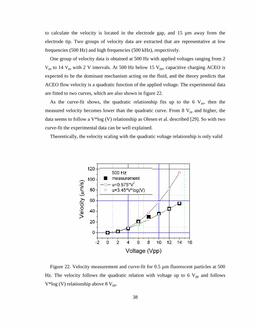
38

to calculate the velocity is located in the electrode gap, and 15 µm away from the

electrode tip. Two groups of velocity data are extracted that are representative at low

frequencies (500 Hz) and high frequencies (500 kHz), respectively.

One group of velocity data is obtained at 500 Hz with applied voltages ranging from 2

Vpp to 14 Vpp with 2 V intervals. At 500 Hz below 15 Vpp, capacitive charging ACEO is

expected to be the dominant mechanism acting on the fluid, and the theory predicts that

ACEO flow velocity is a quadratic function of the applied voltage. The experimental data

are fitted to two curves, which are also shown in figure 22.

As the curve-fit shows, the quadratic relationship fits up to the 6 Vpp, then the

measured velocity becomes lower than the quadratic curve. From 8 Vpp and higher, the

data seems to follow a V*log (V) relationship as Olesen et al. described [29]. So with two

curve-fit the experimental data can be well explained.

Theoretically, the velocity scaling with the quadratic voltage relationship is only valid

Figure 22. Velocity measurement and curve-fit for 0.5 µm fluorescent particles at 500

Hz. The velocity follows the quadratic relation with voltage up to 6 Vpp and follows

V*log (V) relationship above 8 Vpp.

39

for low driving voltage comparable to thermal voltage (~25 mV) as a linear

approximation of zeta potential drops in the double layer. When a higher voltage is

applied, nonlinearity of the electric double layer capacitance would lead measured data to

deviate from the theory prediction. Instead of quadratic relationship, fluid velocity scales

more linearly [27] or even saturates at high voltages. When the voltage is high enough

(15 Vpp or above for my experiments) to induce electrochemical reaction, i.e. Faradaic

charging, corrosion of the electrode and bubble generation prevent the accurate

measurement of the fluid velocity.

Another set of data is obtained at 500 kHz, where the flow velocity is reversed as

compared with the condition at 500 Hz. The tracer particles are 1 µm in diameter. The

applied voltage ranges from 12.5 Vpp to 25 Vpp. ACET velocity scales with the

conductivity of the fluid. For a conductivity of 20 mS/m (tap water) used in the

experiments, which is considered as low for ACET effect, ACET flows are not prominent

until a large voltage is used. The measured velocity for 12.5 Vpp is 3 µm/s and the flows

are merely observed when the voltage is below 10 Vpp. As can be seen from figure 23, the

measured data fits to the third power of voltage (u~V3). Theoretically, ACEO velocity

scales with quadratic relation of the applied voltage, while ACET velocity scales with the

voltage as V2 ~ V4 [30] depending on the heat transfer boundary conditions. So this

indicates that microflows at 500 kHz should be attributed to ACET effect, not ACEO, as

the main driving force. Different boundary conditions and some other side effects would

prevent from reaching theoretical limit in the experiments.

Also, DEP effect contributes to the particle velocity that may not fully represent the

fluid velocity. Larger particles have large DEP force, thus larger DEP velocity. This can

be added to the fluid velocity. So particles with diameter less than 1 µm are preferred

because they contribute less error in measuring the fluid velocity when used as tracers.

3.4 Particle trapping by dielectrophoresis (DEP) using orthogonal electrodes

DEP force acts directly on the particles, instead of fluids. So its function in particle

trapping is to capture particles as holding mechanism after they have been transported to

40

Figure 23. Velocity measurement and curve-fit for 1 µm fluorescent particles at 500

kHz. The velocity fits to the V3 and is compatible with ACET theory prediction.

the detection sites by ACEO or ACET flows.

As discussed above, the DEP force on the spherical particle is given in equation (19),

and DEP velocity is given in equation (22). The magnitude of the velocity depends on the

square of particle size, the permittivity of the suspending medium, and the gradient of the

field strength squared. And it is inverse proportional to the viscosity of the fluid. The sign

of the real part of CM factor decides whether the particle acts as positive or negative

DEP, particles approaching or repelling from the electrodes.

Numerical simulation for DEP velocity field is done in the post-processing step by

Comsol Multiphysics software after solving the electric field distribution. Assume that

the particle is 5 µm in radius, real part of CM factor is 0.5, the applied voltage is 15 Vpp

and fluid viscosity is 0.001. The calculated velocity from equation (22) is given as

follows

2182.95 10DEP rmsv E−⟨ ⟩ = × ∇ (31)

Once the electric field distribution is solved in the simulation, gradient of the field

41

square can be calculated directly using the expression

( _ ^ 2 _ ^ 2, )x ydiff E dc E dc x+ (32)

and ( _ ^ 2 _ ^ 2, )x ydiff E dc E dc y+ (33)

in x and y directions, respectively.

The simulated velocity field is plotted in figure 24. The velocity at the electrode tip is

high where the field gradient is maximized. So particles will accelerate towards the

electrode tip when they are approaching the converging point. Electrode tip is also the

trapping site for the particles experiencing positive DEP force. This prediction is

confirmed by the experimental observations. As equation (31) shows, DEP force decays

rapidly as the electric field strength. The arrows in figure 24 indicate the relative

magnitude of the DEP force, and we can see that DEP force is short-ranged, and is only

effective near the electrode.

Figure 24. Numerical simulation of positive DEP velocity field calculated from the

electric field gradient. The color map shows the electric field strength and the arrows

indicate the relative magnitude of DEP velocity and directions. Particles under positive

DEP effect will converge to the vertical electrode tip, which is the trapping site for

micro/bio particles and cells.

42

In the experiments, various particles and biological cells are tested to see their DEP

effects using orthogonal electrode pair. Sizes of the particles ranges from fluorescent

particles (200 nm, 500 nm), to latex particles (1µm, 3µm) and cells like yeast cells (~5

µm) and algae cells (5-15 µm).

Particles and cells can be trapped at the electrode tip by positive DEP or in the spaces

between the electrodes by negative DEP. Figure 25 is one of the experimental results by

positive DEP. Live yeast cells with average diameter 5 µm were trapped around the

electrode tip with high concentration. The trapping capacity is affected by the electrode

diameter and field strength, as well as the particle type. The picture was taken 5 minutes

after turning on the signal with 1 kHz and 10 Vpp. This kind of particle concentration is

certainly more advantageous over labor intensive culturing that usually takes hours to

days to finish.

Negative DEP effect tends to repel the particles from the electrode surface. For the

orthogonal electrode setup, particles under negative DEP will gather at the gap between

Figure 25. Positive DEP trapping for live yeast cells with average 5 µm in diameter. A

bunch of cells get trapped with high concentration around the electrode tip. The picture

was taken 5 minutes after turning on the signal with 1 kHz and 10 Vpp.

43

the electrodes. Figure 26 is the snapshot of the experiment with algae cells piled in lines

under negative DEP (100 kHz and 10 Vpp). The sizes of the algae cells ranges from 5 to

15 µm.

An interesting phenomenon is the DEP pearl chain formation. Pearl formation is

caused by the electrical dipole moment induced by the ionic polarization of electric

double layer. Positive and negative induced charges distribute at two ends of the cells,

causing attraction between them. Figure 27 shows that latex particles form long chains

near T electrode. The number of particles in a chain can be more than 20. The chains

follow up the direction of the electric field, which is also the direction of the dipole

moment. This is a kind of live indication of how the electric field distributes by

orthogonal electrodes.

From several experiments, it can be concluded that pearl chains normally form by

negative DEP, when particles align along the electric field between the electrodes. Under

positive DEP, particles tend to form groups of clusters instead of pearl chains (Figure 28).

There is a pattern transition from negative DEP to positive DEP. The reverse transition

Figure 26. Negative DEP for live algae cells at 100 kHz and 10 Vpp. Algae cells piled

up in lines around the orthogonal electrode. The direction of the lines follows the electric

field.

44

Figure 27. DEP pearl chains formed around the electrode tips by latex particles. The

picture on the left is taken at 20X objective lens while the picture on the right is the

detailed look at the pearl chain using 100X lens.

Figure 28. Alga cells experience a transition from negative DEP (pearl chains in figure

26, 100 kHz) to positive DEP (clusters at 20 MHz).

45

was never observed, which means that once the clusters are formed, they cannot go back

to form pearl chains again.

As discussed above, both positive and negative DEP are useful in manipulation of

particle and cells. In order to better control particles, such as concentration and separation

of them, it is desirable to know DEP cross-over frequency for different kinds of cells and

particles. DEP cross-over frequency is the frequency at which the cells change moving

directions under non-uniform electric field, which is an important characteristic of bio-

particles.

The transitions from positive to negative DEP or from negative to positive DEP are not

very obvious when observed using orthogonal electrodes. Instead, parallel electrode pairs

are used to get the characteristic frequency point where DEP changes sign. Parallel

electrode pairs, with sharp edges, can easily detect the transition cross-over frequencies.

When the cells experience positive DEP, they are attracted to the edges of the electrodes,

especially the inner edges, where field gradient is strong. When at negative DEP

frequency range, they are repelled from the edges and would gather in the middle of the

parallel electrodes or float above the electrodes. As figure 29 shows, 40/80 electrode

pairs are used to find cross-over frequency of live algae cells. 40/80 means that the

spacing between electrodes is 40 µm and the electrode widths are 80 µm. The frequency

is swept from 100 Hz to 20 MHz by Agilent 33220A signal generator, and cells respond

differently to different frequencies.

The transition frequency is identified at 5 MHz for this type of algae cell. Below this

frequency, the algae cells experience negative DEP. Photos taken at sample frequency

100 Hz, 1 kHz, 100 kHz, and 1 MHz are present in figure 29. At 100 Hz, bubbles are

easily generated by chemical reactions, which would corrode the gold layer on the

electrode. At 1 kHz, cells are swept to the flow null points and piled at two lines on the

electrode surface by strong ACEO flow. At 100 kHz, the cells float above the electrodes

by negative DEP, confined in the middle region of the two electrodes. Cells forming pearl

chains are limited in between the electrodes in large amount at 1 MHz, which indicates

strong negative DEP. Cells stick to the edges of the electrodes by positive DEP at 20

MHz. At this frequency, fewer cells stay between electrodes.

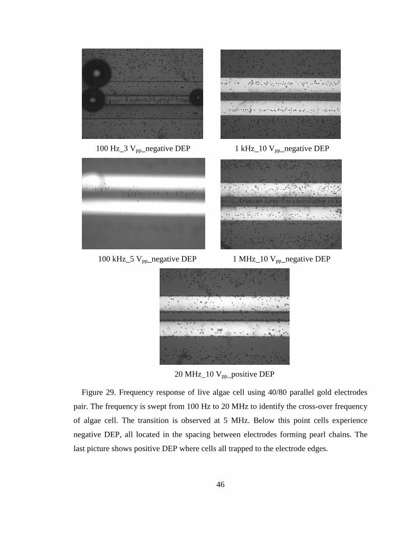
46

100 Hz_3 Vpp_negative DEP 1 kHz_10 Vpp_negative DEP

100 kHz_5 Vpp_negative DEP 1 MHz_10 Vpp_negative DEP

20 MHz_10 Vpp_positive DEP

Figure 29. Frequency response of live algae cell using 40/80 parallel gold electrodes

pair. The frequency is swept from 100 Hz to 20 MHz to identify the cross-over frequency

of algae cell. The transition is observed at 5 MHz. Below this point cells experience

negative DEP, all located in the spacing between electrodes forming pearl chains. The

last picture shows positive DEP where cells all trapped to the electrode edges.

47

3.5 A flow-through system designed for long range particle manipulation

In order to test the particle trapping efficiency, a flow-through system is designed and

fabricated. Figure 30 shows the schematic of the flow-through system. Two platinum

wire electrodes at 500 µm spacing are fitted orthogonally into a sealed PDMS fabricated

channel on a glass slide. PDMS (Polydimethylsiloxane) is the most widely used silicon-

based organic polymer to build micro-channels and chambers. It is optically clear, and is

generally considered to be inert, non-toxic, and non-flammable. As shown in figure 31,

the channel dimension is 1 cm, 0.4 cm, and 0.1 cm by length, width, and height,

respectively. Fluid is pumped in by a programmable syringe pump (NE1000, New Era

Pump System, USA) and flows out to a reservoir. AC signal is applied to electrodes to

generate non-uniform electric field for ACEO, ACET effect, and DEP.

This flow-through system combines both pressure driven flow using syringe pump and

electrokinetic flow generated by orthogonal electrodes excited by AC signal. Particles are

pumped into the chamber with pressure. The electrokinetic flow helps transport particles

to the vicinity of the perpendicular electrode where DEP effect will be stronger to trap

particles. Thus a long range particle manipulation system is created to concentrate and

detect micro/bio particles and cells.

AC

reservoirchannelpump

electrode

Figure 30. Schematic of flow-through system. Two platinum wire electrodes are fitted

into PDMS fabricated channel. Fluid with particles is pumped into the channel by a

programmable syringe pump. AC signal is applied to electrodes to generate non-uniform

electric field for ACEK effect.

48

Figure 31. Device setup of flow-through system. T electrodes in PDMS channel built

on glass slide with inlet and outlet. The channel dimension is 1cm, 0.4cm, and 0.1cm by

length, width, and height, respectively. The spacing between orthogonal electrodes is 500

µm.

The two images in figure 32 show one flow-through result. The experiment condition

is 8 Vpp, 500 kHz with fluid conductivity 0.83 S/m. At flow rate 5 µl/min with initial

concentration 7.5x106 particle/ml, 66% of the algae cells were trapped in the channel

around the electrode tip. The concentration of algae cells in the chamber increased by

30% after 5 minutes. This device works well for particles with low concentration.

According to the above study on fluid flow and DEP characterization, 500 kHz is in the

ACET flow range and negative DEP occurs as cells forms pearl chains. ACET effect

range is chosen instead of ACEO because ACET effect works better for high

conductivity solutions. Particle concentration is calculated by using a counting grid

engraved on glass slides. If the particles are highly concentrated, dilution of the solution

is required to estimate the concentration.

If several flow-through systems cascade together, fluid can be purified with great

efficiency, particularly for low concentration solutions. There are several possible ways

to improve trapping efficiency. First is to find out the optimum frequency to perform

strong DEP effect for different particles/cells. The second is to reduce the flow rate so

particles have more time to settle down. The third method is to modify device parameters

such as spacing, which will change the ACET and DEP strength.

49

Figure 32. One experimental flow-through result. The condition is 8 Vpp, 500 kHz

with fluid conductivity 0.83 S/m. This frequency is in the ACET flow range and negative

DEP occurs for algae cells as they form pearl chains around the electrode tip before (a)

and after (b) applying signal. At flow rate 5 µl/min with initial concentration 7.5x106

particle/ml, 66% of the particles were trapped in the channel, and the concentration of

cells in the chamber increased by 30% after 5 minutes.

50

CHAPTER FOUR: CONCLUSIONS AND FUTURE WORK

The orthogonal electrodes configuration based on AC electrokinetics (ACEK) has

multi-functions for manipulating particles and fluid as well. In the experiments, three

types of microflow fields were observed by changing the applied electric signals. Three

ACEK processes, capacitive electrode polarization (ACEO) for low frequency and low

voltage, Faradaic polarization for low frequency and high voltage, and ACET effect for

high frequency regions are proposed to explain the different flow patterns, respectively.

Well controlled micro-flow (ACEO and ACET flow) help transport target cells to the

trapping site, which greatly enhanced the DEP trapping efficiency. Experiments show

that a large amount of biological cells can be trapped at the electrodes or within the

vicinity of the electrodes by either positive or negative DEP.

Biological cells exhibit different DEP frequency responses according to their own

characteristics. Separating and concentrating of particles can be achieved by studying

single cell property and applying proper conditions. Flow–through system based on

orthogonal electrodes showed promising potential to deal with large volume of low

concentration solutions. Particles can be concentrated to a detectable level for further

processing. DEP combined with ACEK flow show great particle trapping efficiency in

the flow-through system, thus long range particle manipulation is achieved.

Impedance analysis can help choose optimal frequency when implementing ACEO and

ACET effect for fluid manipulation. Equivalent circuit model identifies the relative

impacts of various impedance components at different frequencies and potentials. Finite

element analysis (numerical simulation) helps predict and explain experimental results.

The flow-through system designed using orthogonal electrodes currently combines

pressure driven mechanical pump together with ACEK technique. The orthogonal

electrodes can be micro-fabricated to have well controlled spacing and the chamber can

be sealed by conventional microfabrication techniques used to build chips and MEMS

devices. Mechanical pump can be replaced by ACEK driven micropump to transport

fluid since orthogonal electrodes also showed the potential for pumping effects. The

electro-driven components are more reliable and compatible for integration into lab-on-a-

51

chip devices. This goal requires a lot of future work and research effort.

52

LIST OF REFERENCES

53

LIST OF REFERENCES

[1] H. Morgan and N. G. Green, AC Electrokinetics: Colloids and Nanoparticles

[2] A. Ramos, H. Morgan, N. G. Green, and A. Castellanos, Ac electrokinetics: a review

of forces in microelectrode structures, J. Phys. D: Appl. Phys. 31 (1998) 2338-2353

[3] J. Wu, Interactions of Electrical Fields with Fluids: Laboratory-on-a-chip

Applications, IET Nanobiotechnology, 2(1), pp. 14–27, 2008.

[4] J. Wu, Y. Ben, and H.-C. Chang, Particle detection by electrical impedance

spectroscopy with asymmetric-polarization AC electroosmotic trapping, Microfluid

Nanofluid (2005) 1: 161–167

[5] M. R. Brown and C. D. Meinhart, AC electroosmotic flow in a DNA concentrator,

Microfluid Nanofluid (2006) 2: 513–523

[6] N. Islam and J. Wu, Microfluidic Transport by AC Electroosmosis, Journal of

Physics: Conference Series 34 (2006) 356–361

[7] D. Lastochkin, R. Zhou, P. Wang, Y. Ben, and H.-C. Chang, Electrokinetic

micropump and micromixer design based on ac faradaic polarization, J. Appl. Phys.,

Vol. 96, No. 3, 1 August 2004

[8] N. G. Green, A. Ramos, A. González, A. Castellanos, and H. Morgan, Electric field

induced fluid flow on microelectrodes: the effect of Illumination, J. Phys. D: Appl.

Phys. 33 (2000) L13–L17

[9] M. Lian, N. Islam, and J. Wu, AC Electrothermal Manipulation of Conductive Fluids

and Particles for Lab-chip Applications, IET Nanobiotechnology, 1(3), pp. 36-43.

2007

[10] J. Wu, M. Lian, and K. Yang, Micropumping of Biofluids by AC Electrothermal

Effects, Appl. Phys. Lett., 90, 234103, 2007

[11] M. Sigurdson, D. Wang, and C. D. Meinhart, Electrothermal stirring for

heterogeneous immunoassays, Lab on a chip, 2005, VOL 5; NUMB 12, pages 1366-

1373

54

[12] D. Wang, M. Sigurdson, and C. D. Meinhart, Experimental analysis of particle and

fluid motion in ac electrokinetics, Experiments in Fluids 38 (2005) 1–10

[13] A. Ramos, H. Morgan, N.G. Green, A. Gonzalez, and A. Castellanos, Pumping of

liquids with traveling-wave electroosmosis, J. Appl. Phys. 97, 084906, 2005.

[14] J. Wu and H.-C. Chang, Asymmetrically Biased AC Electrochemical Micropump,

AIChE annual meeting 2004, Nov. 7 – 12, Austin, TX

[15] A.B.D. Brown, C.G. Smith, and A.R. Rennie, Pumping of water with ac electric

fields applied to asymmetric pairs of microelectrodes, Phys. Rev. E 63, 016305,

2000.

[16] J.P. Urbanski, T. Thorsen, J.A. Levitan, and M.Z. Bazant, Fast ac electro-osmotic

micropumps with nonplanar electrodes, Appl. Phys. Lett. 89, 143508, 2006.

[17] R. Pethig, R. S. Lee, and M. S. Talary, Cell Physiometry Tools based on

Dielectrophoresis, BioMEMS and Biomedical Nanotechnology, Volume II:

Micro/Nano Technologies for Genomics and Proteomics

[18] R. Pethig, Dielectrophoresis of Biological Cells, Encyclopedia of Surface and

Colloid Science, Pp. 1719-1736, 2006, Taylor & Francis

[19] H. Morgan, D. Holmes, and N.G. Green, 3D focusing of nanoparticles in

microfluidic channels, IEE Proc.-Nanobiotechnol. Vol. 150, No. 2, November 2003

[20] D. Holmes, N. G. Green, and H. Morgan, Microdevices for Dielectrophoretic Flow-

Through Cell Separation, IEEE Engineering In Medicine and Biology Magazine,

November/December 2003

[21] Z. Gagnon and H.-C. Chang, Aligning fast alternating current electroosmotic flow

fields and characteristic frequencies with dielectrophoretic traps to achieve rapid

bacteria detection, Electrophoresis 2005, 26, 3725–3737

[22] H.-C. Chang, Electro-Kinetics: A Viable Micro-Fluidic Platform for Miniature

Diagnostic Kits, the Canadian Journal of Chemical Engineering, volume 84, APRIL

2006

[23] J. A. Wood, B. Zhang, M. R. Tomkins, and A. Docoslis, Numerical investigation of

AC electrokinetic virus trapping inside high ionic strength media, Microfluid

Nanofluid (2007) 3:547–560

55

[24] A. R. Minerick, R. Zhou, P. Takhistov, and H.-C. Chang, Manipulation and

characterization of red blood cells with alternating current fields in microdevices,

Electrophoresis 2003, 24, 3703-3717

[25] P. Y. Chiou, A. T. Ohta, and M. C. Wu, Massively parallel manipulation of single

cells and microparticles using optical images, nature, Vol436, 21 July 2005

[26] N.G. Green, A. Ramos, A. González, H. Morgan, and A. Castellanos, Fluid flow

induced by nonuniform ac electric fields in electrolytes on microelectrodes. III.

Observation of streamlines and numerical simulation, Phys. Rev. E 66, 026305

(2002)

[27] V. Studer, A. Pepin, Y. Chen, and A. Ajdari, An integrated AC electrokinetic pump

in a microfluidic loop for fast and tunable flow control, Analyst, 2004, 129, pp. 944-

949.

[28] J. Wu, Y. Ben, D. Battigelli, and H.-C. Chang, Long-Range AC Electroosmotic

Trapping and Detection of Bioparticles, Industr. Eng. Chem. Research, 2005, 44(8),

pp. 2815 – 2822.

[29] L. H. Olesen, H. Bruus, and A. Ajdari, ac electrokinetic micropumps: The effect of

geometrical confinement, Faradaic current injection, and nonlinear surface

capacitance, Phys. Rev. E 73, 056313 (2006)

[30] A. Castellanos, A. Ramos, A. González, N.G. Green, and H. Morgan,

Electrohydrodynamics and dielectrophoresis in microsystems: scaling laws, J. Phys.

D: Appl. Phys. 36 (2003) 2584-2597

56

VITA

Kai Yang was born in Zhangjiagang, Jiangsu Province, People’s Republic of China

(PRC), on October 14, 1982. He went to Shanghai Jaiotong University after graduation

from high school in 2001 and received B.S. in Electronics Science and Technology in

2005. He came to the US in 2006 for graduate study at the University of Tennessee,

Knoxville and received M.S. in Electrical Engineering in spring, 2008.

Kai Yang is currently pursuing his doctorate in Electrical Engineering at The

University of Tennessee, Knoxville, TN, USA.