Absorbing boundary conditions for the two-dimensional

Schrodinger equation with an exterior potential.

Part I: construction and a priori estimates ∗

Xavier Antoine† Christophe Besse‡ Pauline Klein§

Abstract

The aim of this paper is to construct some classes of absorbing boundary conditions for thetwo-dimensional Schrodinger equation with a time and space varying exterior potential and forgeneral convex smooth boundaries. The construction is based on asymptotics of the inhomogeneouspseudodifferential operators defining the related Dirichlet-to-Neumann operator. Furthermore, apriori estimates are developed for the truncated problems with various increasing order boundaryconditions. The effective numerical approximation will be treated in a second paper.

Contents

1 Introduction 2

2 What we already know and what remains true compared to the one-dimensionalcase 42.1 The half-space case and a null potential . . . . . . . . . . . . . . . . . . . . . . . . . . 42.2 The time dependent potential case . . . . . . . . . . . . . . . . . . . . . . . . . . . . . 4

3 Specific aspects of the two-dimensional case 53.1 Choice of the boundary and local parameterization . . . . . . . . . . . . . . . . . . . . 53.2 Discussion on the equivalence between the two strategies . . . . . . . . . . . . . . . . . 63.3 Pseudodifferential operator calculus for the 2D case . . . . . . . . . . . . . . . . . . . . 73.4 E-quasi hyperbolic, elliptic and glancing zones . . . . . . . . . . . . . . . . . . . . . . 8

∗The authors are partially supported by the French ANR fundings under the project MicroWave NT09 460489.†Institut Elie Cartan Nancy, Nancy-Universite, CNRS UMR 7502, INRIA CORIDA Team, Boulevard des Aiguillettes

B.P. 239, F-54506 Vandoeuvre-les-Nancy, France (Xavier.Antoine@iecn.u-nancy.fr).‡Laboratoire Paul Painleve, Universite Lille Nord de France, CNRS UMR 8524, INRIA SIMPAF Team,

Universite Lille 1 Sciences et Technologies, Cite Scientifique, 59655 Villeneuve d’Ascq Cedex, France.(Christophe.Besse@math.univ-lille1.fr).§Laboratoire de Mathematiques de Besancon, CNRS UMR 6623, Universite de Franche-Comte, 16 route de Gray,

25030 Besancon, France. (Pauline.Klein@iecn.u-nancy.fr).

1

4 Two possible strategies 94.1 Strategy I: gauge change method . . . . . . . . . . . . . . . . . . . . . . . . . . . . . . 94.2 Strategy II: direct method . . . . . . . . . . . . . . . . . . . . . . . . . . . . . . . . . . 104.3 Unification of the strategies . . . . . . . . . . . . . . . . . . . . . . . . . . . . . . . . . 104.4 Symbolic system . . . . . . . . . . . . . . . . . . . . . . . . . . . . . . . . . . . . . . . 104.5 Adding terms in the principal symbol . . . . . . . . . . . . . . . . . . . . . . . . . . . 13

5 Strategy I: gauge change 145.1 Choice of the principal symbol . . . . . . . . . . . . . . . . . . . . . . . . . . . . . . . 145.2 Symbols computation . . . . . . . . . . . . . . . . . . . . . . . . . . . . . . . . . . . . 155.3 Interpretation of the ABCs for the Taylor approach . . . . . . . . . . . . . . . . . . . . 165.4 Interpretation of the ABCs for the Pade approach . . . . . . . . . . . . . . . . . . . . 19

6 Strategy II: direct method 206.1 Computation of the symbols . . . . . . . . . . . . . . . . . . . . . . . . . . . . . . . . . 216.2 Interpretation of the ABCs for the Taylor approach . . . . . . . . . . . . . . . . . . . . 226.3 Interpretation of the ABCs and Pade approach . . . . . . . . . . . . . . . . . . . . . . 23

7 A priori estimates 267.1 Principle . . . . . . . . . . . . . . . . . . . . . . . . . . . . . . . . . . . . . . . . . . . . 267.2 A priori estimates for ABCM

2,T . . . . . . . . . . . . . . . . . . . . . . . . . . . . . . . 27

7.3 A priori estimates for ABCM1,T . . . . . . . . . . . . . . . . . . . . . . . . . . . . . . . 31

8 Conclusion 33

1 Introduction

The aim of this paper is to propose some Absorbing Boundary Conditions (ABCs) for the two-dimensional linear time-dependent Schrodinger equation [1] with a potential V

i∂tu+ ∆u+ V (x, y, t)u = 0, (x, y) ∈ R2, t > 0

u(x, y, 0) = u0(x, y), (x, y) ∈ R2,(1)

where u0 ∈ L2(R2) is compactly supported in the future bounded spatial computational domain Ω,with fictitious boundary Σ. The potential function is C∞, space and time dependent and real-valued.We assume that the smoothness of V is at least satisfied outside ΣT := Σ×]0;T [, T being the finaltime of computation. The computational domain is ΩT = Ω×]0;T [. Under suitable conditions, theinitial boundary value problem (1) is well-posed [12, 13]. Moreover, in the free-space the L2-norm ofthe solution is conserved

∀t > 0, ‖u(t)‖2L2(R2) =

∫R2

|u(x, y, t)|2dxdy = ‖u0‖2L2(R2) (2)

where ‖·‖2L2(R2) is the L2(R2)-norm. Finally, n is the outwardly directed unit normal vector to Σ.

2

The main difficulty here in designing ABCs is that we include a general potential V := V (x, y, t). Inpractical applications, being able to handle correctly potential effects is an important, active and notcompletely understood topic in physics [23, 15, 14, 21, 22]. Here, we assume that the potential makesthe wave outgoing to the bounded domain Ω. In the one-dimensional case, a sufficient condition is thatV is an acceleration or a repulsive potential [5]. Examples of potentials which cannot be considered arethe confining potentials. In the two-dimensional case, a definition of admissible (repulsive) potentialdoes not exist. For this reason, we assume that the outgoing wave assumption holds without givinga mathematical definition. This point is probably interesting and important to discuss but also outof the scope of the paper. Our contribution focuses on the effective construction of ABCs and someof their properties. Their discretization and numerical comparison will be included in a companionpaper [6].

In the one-dimensional case, ABCs for some special time independent potentials can be obtainedvia explicit calculations of the Dirichlet-to-Neumann (DtN) operator by using special functions (forexample Airy’s functions) [20, 19] or particular techniques (Floquet’s theory for sinusoidal potentials[29]). Handling general potentials can be achieved by using pseudodifferential operator theory andsymbolic asymptotic expansions of the DtN map. In [5], we introduced two strategies to build robustand accurate ABCs making use of the Engquist & Majda [16, 17] approach adapted to the Schrodingerequation [5, 7, 3, 1, 8, 25, 26, 18, 11]. In the present paper, we develop the extension of the theory tothe two-dimensional case for general smooth convex boundaries Σ. As we will see, the two strategiesof the one-dimensional case can be extended to the two-dimensional case. However, since the principalsymbol of the DtN operator is more complicated, further (high frequency) asymptotic expansions arerequired and lead in fact to four families of ABCs, two for each strategy. After designing these ABCs,we also investigate the obtention of a priori estimates, which from the semi discrete point of viewwould correspond to prove stability of the discretization schemes. Let us note that the technique ofPerfectly Matched Layer (PML) [10] can also be used to bound the computational domain for spatiallydependent potentials. We refer to [28] for more details.

The paper is structured as follows. In the second Section, we review some results known for specialtwo-dimensional problems and explain what can be extended from the one- to the two-dimensionalcase. In Section 3, we introduce a local parameterization of the boundary and discuss the possiblelinks between the two strategies. Next, specific pseudodifferential operators results are summarizedand the E-quasi hyperbolic, elliptic and glancing zones are defined. In Section 4, we explain in detailsthe two strategies. The first one (strategy I) is called the gauge change and the second one (strategyII) is the direct method. We unify the notations and then develop the symbolic system which givesthe asymptotic expansion of the total symbol of the DtN map. We then discuss the choice of theprincipal symbol of the DtN map which plays a key role in the accuracy of the ABCs. Section 5 dealswith the gauge change strategy (strategy I) where we detail the calculations and the construction ofABCs. Section 6 does the same developments but for the direct strategy (strategy II). We state apriori estimates in Section 7 and conclude in Section 8.

3

2 What we already know and what remains true compared to theone-dimensional case

2.1 The half-space case and a null potential

Let us consider the positive half-space x > 0. We set Ω := x < 0 with boundary Σ = x = 0.Let us assume that the potential V is equal to zero in the right half-space. Then we can prove thatthe (exact) Transparent Boundary Condition (TBC) for the problem

i∂tu+ ∂2xu+ ∂2

yu+ V u = 0, (x, y) ∈ R2, t > 0,

is given by the Dirichlet-to-Neumann (DtN) map

∂nu− i√i∂t + ∆Σ u = 0, (x, y) ∈ ΣT . (3)

This TBC can be obtained by Fourier transform in time t and space y. Then, the resulting differentialequation in x is solved explicitly leading to the linear combination of two traveling waves. It is nextsufficient to kill the incoming wave and to derive according to x (normal derivative ∂n := ∂x) to get(3) in the (y, t) Fourier space. An inverse Fourier transform then gives the result. In our case, theLaplace-Beltrami operator ∆Σ is ∂2

y . The transparent operator is given by a square-root Schrodingeroperator on the boundary Σ. This operator is nonlocal in time and space. We will see later that thisoperator can be localized (for example by a Taylor expansion) or globally localized in time and space(through rational approximants [6]).

2.2 The time dependent potential case

In the one-dimensional case and when the potential is only time dependent V (x, t) = V (t) outsideΩ, a gauge change leads to work with a free potential Schrodinger equation. If u is solution to:i∂tu+ ∂2

xu+ V (t)u = 0, and v is defined by

v(x, t) = u(x, t)e−i∫ t0 V (s)ds,

then v is solution to: i∂tv + ∂2xv = 0, for which the TBC is known. In the two-dimensional case, this

property remains true. If V (x, y, t) = V (t) and u is solution to

i∂tu+ ∂2xu+ ∂2

yu+ V (t)u = 0,

then, by defining

v(x, y, t) = u(x, y, t)e−i∫ t0 V (s)ds, (4)

v is solution to the free potential equation: i∂tv + ∂2xv + ∂2

yv = 0. This result is independent of thecoordinates system (x, y).

4

3 Specific aspects of the two-dimensional case

3.1 Choice of the boundary and local parameterization

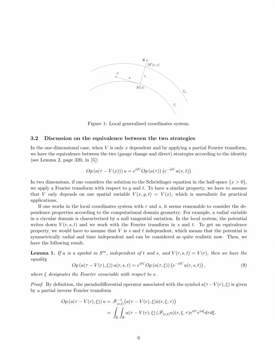
Let us consider a rectangular domain Ω parameterized in cartesian coordinates (x, y) with corners(x1, y1), (x1, y2), (x2, y2) and (x2, y1). For the vertical right boundary Σr = (x, y) ∈ R2/x = x2, y ∈[y1; y2], we use the pseudodifferential operator calculus associated with the partial Fourier transformin (y, t) to get the DtN operator according to ∂x by considering the right half-space. Then, we obtain aTBC on Σd. The problem is that this boundary condition is singular at (x2, y2) and does not smoothlymatch with the boundary condition that one would get on Σh := [x1;x2]×y2 by considering a partialFourier transform in (x, t). This means that additional continuity conditions at the corners must bedeveloped (see e.g. [27] for the wave equation). To the best of our knowledge, this question hasnot been treated yet for the Schrodinger equation. Furthermore, to have an outgoing solution to thecomputational domain Ω, a convex (regular) boundary Σ must be considered. Therefore, we try towrite a boundary condition on a smooth (closed) convex boundary Σ parameterized by its curvilinearabscissa s ∈ [a; b]. The assumption about the convexity implies that the local curvature at s, κ = κ(s),is positive.

Let Ω be a convex domain with smooth boundary Σ. We do not detail here all the calculationsand refer to [3] for more explanations concerning the change of variables. For a point M of Σ withcoordinates (x, y), we designate by τ the tangential vector to Σ at M and n the outwardly directedunit normal vector. In the local coordinates system associated with M , a point M ′ close to theboundary is connected to its coordinates r and s. Since Ω is convex, the projection of the point M ′

onto the boundary Σ is unique, giving hence its curvilinear abscissa s. The radial coordinate r is thedistance from point M ′ to its projection according to the outgoing unitary normal vector. Hence, Σcan be denoted by Σ0, if Σr designates the parallel surface to Σ at distance r. Since Σ is convex,we can restrict ourselves to positive values of r, bounded from above by a small parameter ε, and sor ∈ [0; ε]. The laplacian in local coordinates (r, s) writes down [4, 2]

∆r = ∂2r + κr∂r + h−1∂s(h

−1∂s), (5)

with the scaling factor h: h = 1+rκ and κr the curvature at M ′ on the parallel surface Σr: κr = h−1κ.For the sake of conciseness, we denote by u the function u written in the local system

u(x, y, t) = u(r, s, t), (x, y) ∈ R2, (r, s) ∈ [0; ε]× [a; b], t > 0, (6)

and Vr the locally rewritten potential function

V (x, y, t) = Vr(r, s, t), (x, y) ∈ R2, (r, s) ∈ [0; ε]× [a; b], t > 0. (7)

The Schrodinger equation for system (1) is then

i∂tu+ ∂2r u+ κr∂ru+ h−1∂s(h

−1∂s)u+ Vru = 0, (r, s, t) ∈ [0; ε]× [a; b]×]0;T ], (8)

where r and s parameterize the domain Ω and t > 0. In the sequel, we identify u to u.

5

M(s)

Σ

~τs

~n

Σr

r

M ′(r, s)

Figure 1: Local generalized coordinates system.

3.2 Discussion on the equivalence between the two strategies

In the one-dimensional case, when V is only x dependent and by applying a partial Fourier transform,we have the equivalence between the two (gauge change and direct) strategies according to the identity(see Lemma 2, page 320, in [5])

Op (a(τ − V (x)))u = eitVOp (a(τ))(e−itV u(x, t)

)In two dimensions, if one considers the solution to the Schrodinger equation in the half-space x > 0,we apply a Fourier transform with respect to y and t. To have a similar property, we have to assumethat V only depends on one spatial variable V (x, y, t) = V (x), which is unrealistic for practicalapplications.

If one works in the local coordinates system with r and s, it seems reasonable to consider the de-pendence properties according to the computational domain geometry. For example, a radial variablein a circular domain is characterized by a null tangential variation. In the local system, the potentialwrites down V (r, s, t) and we work with the Fourier transform in s and t. To get an equivalenceproperty, we would have to assume that V is s and t independent, which means that the potential issymmetrically radial and time independent and can be considered as quite realistic now. Then, wehave the following result.

Lemma 1. If a is a symbol in Sm, independent of t and s, and V (r, s, t) = V (r), then we have theequality

Op (a(τ − V (r), ξ))u(r, s, t) = eitVOp (a(τ, ξ))(e−itV u(r, s, t)

), (9)

where ξ designates the Fourier covariable with respect to s.

Proof. By definition, the pseudodifferential operator associated with the symbol a(τ−V (r), ξ) is givenby a partial inverse Fourier transform

Op (a(τ − V (r), ξ))u = F−1(s,t)

(a(τ − V (r), ξ)u(r, ξ, τ)

)=

∫R

∫Ra(τ − V (r), ξ) (F(s,t)u)(r, ξ, τ)eitτeisξdτdξ.

6

By using the following time variable change ρ = τ − V (r) one gets

Op (a(τ − V (r), ξ))u =

∫R

∫Ra(ρ, ξ) (F(s,t)u)(r, ξ, ρ+ V (r)) eitρeitV (r)eisξdρdξ.

From the translation properties of the Fourier transform we can simplify the expression

Op (a(τ − V (r), ξ))u = eitV (r)

∫R

∫Ra(ρ, ξ) F(s,t)((r, s, t) 7→ e−itV (r)u(r, s, t))(r, ξ, ρ) eitρeisξdρdξ.

Then, we identify the operator with symbol a(ρ, ξ) applied to the function (r, s, t) 7→ e−itV (r)u(r, s, t),i.e.

Op (a(τ − V (r), ξ))u = eitV (r)Op (a(τ), ξ)(e−itV (r)u(r, s, t)

),

which proves (9).

3.3 Pseudodifferential operators for the two-dimensional case and associated sym-bolic calculus

The functions that we consider in this chapter depend not only on two variables, the local spatialcoordinates r and s, but also on the time t. In this framework, the two-dimensional pseudodifferentialoperator calculus is realized through the partial Fourier transform (s, t) of a function f(r, s, t). Wedenote by ξ (respectively τ) the covariable of s (respectively t). We have

F(s,t) (f(r, s, t)) (r, ξ, τ) =1

4π2

∫R

∫Rf(r, s, t)e−itτe−isξdtds (10)

and we set F = F(s,t) in this section. A pseudodifferential operator P (r, s, t, ∂s, ∂t) with symbolp(r, s, t, ξ, τ) is defined by

P (r, s, t, ∂s, ∂t)u(r, s, t) = F−1(s,t)

(p(r, s, t, ξ, τ)u(r, ξ, τ)

), (11)

that is

P (r, s, t, ∂s, ∂t)u(r, s, t) =

∫R

∫Rp(r, s, t, ξ, τ)u(r, ξ, τ)eitτeisξdτdξ (12)

where u = Fu.The inhomogeneous pseudodifferential operator calculus that we use in the paper was introduced

in [18] and applied e.g. in [3]. For the sake of conciseness, we only give the useful material neededhere. Let m be a real number and O an open subset of R2. Then (see in [24]), the symbol classSm(O×R+) denotes the linear space of C∞ functions a(r, s, t, τ, ξ) in O×R+×R2 such that for eachK ⊆ O and for all integer indices k, αr, αs, l and β, there exists a constant Ck,αr,αs,l,β(K) such that

|∂kt ∂αrr ∂αs

s ∂lτ∂βξ a(r, s, , t, τ, ξ)| ≤ Ck,αr,αs,l,β(K)(1 + τ2 + ξ4)m−β−2,

for all (r, s) ∈ K, t ∈ R+ and (τ, ξ) ∈ R2.Let E = (1, 2). The homogeneity of a pseudodifferential operator can be deduced from the ho-

mogeneity of its symbol with respect to (ξ2, τ). Therefore, ξ2 and τ are considered as homogeneous[18, 11]. This leads to the following definition.

7

Definition 1. A function f(r, s, t, ξ, τ) is said to be E-quasi homogeneous of order m if and only iffor all µ > 0 and for large (ξ2, τ) we have

f(r, s, t, µξ, µ2τ) = µm f(r, s, t, ξ, τ). (13)

For example, the operator with symbol λ =√−τ − ξ2 is first order E-quasi homogeneous (with

respect to (ξ2, τ)).From now on, a E-quasi homogeneous pseudodifferential operator of order m ∈ Z, denoted by

A ∈ OPSmE , is defined as an operator with a total symbol a(r, s, t, ξ, τ) admitting an asymptoticexpansion in E-quasi homogeneous symbols

a(r, s, t, ξ, τ) ∼+∞∑j=0

am−j(r, s, t, ξ, τ), (14)

where the functions am−j , j ∈ N, are E-quasi homogeneous of degree m − j. The meaning of ∼ in(14) is here

∀m ∈ N, a−m∑j=0

pm−j ∈ Sm−(m+1)E . (15)

A symbol a satisfying the property (14) is denoted by a ∈ SmE and the associated operators A = Op(a)by A ∈ OPSmE . Finally, we introduce OPS−∞E as the intersection between all the classes OPSmE , m ∈ Z.For P and Q two pseudodifferential operators with respective symbols p and q, and m ∈ Z, we set

P = Q mod OPSmE (16)

or equivalentlyp = q mod SmE (17)

if the difference between the two symbols fulfills: p − q ∈ SmE . Finally, the composition formula fortwo operators A and B with respective symbols σ(A) and σ(B) writes

σ(AB) =

+∞∑|α|=0

(−i)|α|

α!∂α(ξ,τ)σ(A) ∂α(s,t)σ(B). (18)

Furthermore, if σ(A) ∈ SmE and σ(B) ∈ SnE , then we have σ(AB) ∈ Sm+nE . In (18), α is a multi-index

(α1, α2). We use the classical notations for multi-indices. In particular, its length |α| is defined by:|α| = α1 + α2. The factorial is defined by: α! = α1!α2!, and we introduce the derivative according to(ξ, τ): ∂α(ξ,τ)λ = ∂α1

ξ ∂α2τ λ(r, s, t, ξ, τ). These classes of operators allows to define an associated symbolic

calculus [18, 11]. Finally, we have: σ(∂s) = iξ and σ(∂2s ) = −ξ2.

3.4 E-quasi hyperbolic, elliptic and glancing zones

Let us recall that the ABCs will be built in the high frequency regime. More precisely, we considerthe following definition with E = (1, 2) [7].

8

Definition 2. We define the E-quasi hyperbolic zone as the set H of points (s, t, ξ, τ) such that

H = (s, t, ξ, τ),−τ − ξ2 > 0 (19)

The construction of the ABCs is then realized under the microlocal assumption that the points(s, t, ξ, τ) lie in H. This hypothesis characterizes the propagative part of the wave. Two other regionscan be also defined: the E-quasi elliptic zone E given by

E = (s, t, ξ, τ),−τ − ξ2 < 0, (20)

which gives the evanescent (exponentially decaying) part of the wave and the E-quasi glancing zonewhich is the complementary set G of E ∪H. This last region is reduced to 0 if u is not tangentiallyincident to Σ. We always assume here that the frequencies are defined in H. This assumption is notalways valid but is true if we suppose that the evanescent part is reduced to 0.

4 Two possible strategies

To build the asymptotic expansion of the DtN operator on Σ, we factorize the Schrodinger operatorwith Nirenberg’s techniques [24] in the generalized system (r, s) given by (8). This allows us, as inthe one-dimensional case, to obtain the DtN pseudodifferential operators Λ− and Λ+ characterizingrespectively the incoming and outgoing wave. Two strategies can then be followed according to thefact that the gauge change is applied or not. In each case, we are going to explicit the underlyingSchrodinger operator on which a factorization is made.

4.1 Strategy I: gauge change method

The first strategy that we consider consists in applying the gauge change before building the boundarycondition. Let us recall that the change of unknown (4) leads to the TBC for a potential V = V (t)and a half-space. Let us introduce the phase function V

V(r, s, t) =

∫ t

0Vr(r, s, σ)dσ, (21)

and do the change of unknownv(r, s, t) = e−iV(r,s,t)u(r, s, t). (22)

Then, the new function v is solution to the variable coefficients Schrodinger equation

i∂tv + ∂2rv +

(κr + 2i(∂rV)

)∂rv + h−1∂s(h

−1∂s) + 2i(∂sV)∂sv +Gv = 0, (23)

where G is the zero order operator given by

G = iκr(∂rV) + i∂2rV − (∂rV)2 + i∂2

sV − (∂sV)2 + ih−1(∂sh−1)(∂sV). (24)

Hence, after the gauge change, function v is solution to

L(r, s, t, ∂s, ∂t)v = 0, on ΩT ,

with L defined by

L = i∂t + ∂2r +

(κr + 2i(∂rV)

)∂r + h−1∂s(h

−1∂s) + 2i(∂sV)∂s +G. (25)

9

4.2 Strategy II: direct method

The second strategy consists in directly working on the operator involved in (8), that is

L = i∂t + ∂2r + κr∂r + h−1∂s(h

−1∂s) + Vr. (26)

Unlike the gauge change method, a term related to the potential will be handled in the principalsymbol Λ+.

Remark 1. As in the one-dimensional case, the difference between the two strategies is related to twopoints. First, the gauge change (22) is only applied in the first strategy while we directly work on uin the second method. However, a second difference concerns the choice of the principal symbol. Inthe direct method, and unlike the gauge change, zero order terms are included in the principal symbolto compensate the gauge change effect. Following this strategy, another strategy, called strategy 0,which is more basic may be considered. This aproach would consist in neither applying the gaugechange nor taking the potential into the principal symbol. However, like the one-dimensional case andas seen later (see Remark 4, page 23), this strategy corresponds to a high frequency approximation,for large |τ |, of strategy II via a Taylor expansion. We note that this is however the approach used in[4, 7].

4.3 Unification of the strategies

In a unified framework, we are now led to build a boundary condition for the Schrodinger equationwith variable coefficients A and B(

i∂t + ∂2r + (κr +A) ∂r + h−1∂s(h

−1∂s) +B)w = 0, on ΩT , (27)

where A and B and the unknown w differ according to strategy I or II. For the gauge change, theunknown is w = v = e−iVu and

A = 2i(∂rV), B = 2i(∂sV)∂s +G. (28)

For the direct method, the unknown is w = u and the coefficients are

A = 0, B = Vr. (29)

4.4 Symbolic system

The operator L associated with the general equation (27) writes down

L = i∂t + ∂2r + (κr +A) ∂r + h−1∂s(h

−1∂s) +B (30)

where the operators A and B are given by either (28) or (29). We have the following factorizationtheorem.

Theorem 1. Let L be the Schrodinger operator with coefficients (30). There exist two first-order ho-mogeneous classical pseudodifferential operators Λ± = Λ±(r, s, t, ∂s, ∂t) ∈ OPS 1

E, smoothly dependentwith respect to r, and such that

L(r, s, t, ∂s, ∂t) = (∂r + iΛ−)(∂r + iΛ+) +R (31)

10

where R = R(r, s, t, ∂s, ∂t) is a smoothing operator in OPS−∞E . Furthermore, the total symbol λ± =σ(Λ±) of Λ± admits an asymptotic expansion in E-quasi homogeneous symbols

σ(Λ±) = λ± ∼+∞∑j=0

λ±1−j (32)

where λ±1−j ∈ S1−jE for j ∈ N. These asymptotic expansions are unique once the principal symbols λ±1

are fixed.

Proof. To prove the result, we develop the expression (31) of L and group together the terms indecaying power of ∂r

L = ∂2r + iΛ−∂r + i∂rΛ

+ − Λ−Λ+ +R.

By using the identity ∂rΛ+ = Λ+∂r +Op (∂rλ

+), we deduce

L = ∂2r + i(Λ+ + Λ−)∂r + iOp

(∂rλ

+)− Λ−Λ+ +R. (33)

Then, we can compare (30) and (33) and identify the terms of the same order in ∂r in the twoexpressions, modulo the smoothing operator R of order −∞. We obtain the system

i(Λ+ + Λ−) = κr +A

iOp(∂rλ

+)− Λ−Λ+ = i∂t + h−1∂s(h

−1∂s) +B.(34)

The term h−1∂s(h−1∂s) can be developed as

h−1∂s(h−1∂s) = h−1h−1∂2

s + h−1∂s(h−1)∂s (35)

implying that the symbol of this operator is

σ(h−1∂s(h

−1∂s))

= −h−2ξ2 + ih−1∂s(h−1)ξ.

Furthermore, the symbol of Λ−Λ+ being given by (18), (34) leads to the symbolic system

i(λ+ + λ−) = κr + a

i∂rλ+ −

+∞∑|α|=0

(−i)|α|

α!∂α(ξ,τ)λ

−∂α(s,t)λ+ = −τ − h−2ξ2 + ih−1(∂sh

−1)ξ + b(36)

where a = A and b = B, respectively, designate the symbols of the operators A and B, respectively.In the gauge change case, we have

a = 2i(∂rV), b = −2(∂sV)ξ + g, (37)

where g = G is the zero order operator defined by (24); for the direct method, the symbols are givenby

a = 0, b = Vr. (38)

We now have to determine the asymptotic expansion in E-quasi homogeneous symbols of the totalsymbol λ+. This asymptotic expansion is obtained by identifying in (36) the terms of the same order

11

of homogeneity. Before that, system (36) can be reduced to one unknown, λ+. Indeed, the term aonly depends on r, s and t,but not of ξ, nor τ . We first extract λ− from the first equation

λ− = −λ+ − iκr − ia.

This expression is then injected into the second equation. But, as the terms κr and a do not dependneither on τ nor on ξ, we have

∂α(ξ,τ)λ− =

−λ+ − iκr − ia if α = 0

−∂α(ξ,τ)λ+ if |α| > 1.

In the infinite sum of the second equation of (36), the terms can be written as

∂α(ξ,τ)λ−∂α(s,t)λ

+ =

−λ+λ+ − iκrλ+ − iaλ+ if α = 0

−∂α(ξ,τ)λ+∂α(s,t)λ

+ if |α| > 1.

Hence, the second equation of (36) gives

i∂rλ+ + iκrλ

+ + iaλ+ ++∞∑|α|=0

(−i)|α|

α!∂α(ξ,τ)λ

+∂α(t,r)λ+ = −τ − h−2ξ2 + ih−1(∂sh

−1)ξ + b. (39)

This last equation will be the starting point to get the symbols λ+1−j , j ∈ Z, which in each case lead

to an approximate boundary condition.

The factorization (31) indicates that the reflected part of the wave is given by w+ = (∂n + iΛ+)w.The TBC is then

w+ = (∂n + iΛ+)w = 0, on ΣT , (40)

where the pseudodifferential operator Λ+ is defined by

Λ+ = Λ+|r=0. (41)

Like Λ+, the operator Λ+ can be developed in homogeneous symbols and its expansion is given by

σ(

Λ+)∼

+∞∑j=0

λ1−j (42)

whereλ1−j =

(λ+

1−j

)|r=0

. (43)

As a consequence, determining the operator Λ+ requires the computation of its boundary symbols:

(λ+1−j)|r=0. We approximate Λ+ by truncating its asymptotic expansion (42). Keeping its first M

terms (λ1−j)0≤j≤M−1, the approximate boundary condition of order M writes down

∂nwM + i

M−1∑j=0

Op(λ1−j

)wM = 0, on ΣT ,

12

where wM is then an approximate solution to (27). In the gauge change case, we then apply the inversechange of unknown w = e−iVu to express the approximate boundary condition on uM . The questionis now how to compute the first M symbols of the asymptotic expansion of λ+, for each strategy andfinally evaluating the symbols on the boundary for r = 0.

4.5 Adding terms in the principal symbol

We can classify the terms appearing in the right hand side of (39) in three classes: the second orderterms, which must be included in the principal symbol; the potential type terms of order zero whichwill be considered in the principal symbol only for strategy II; and some first order terms that may beincluded or not into the principal symbol for both strategies. The key argument allowing to determineif a term may be included in the principal symbol is related to the sign of the imaginary part of λ+

1

which guarantees that the wave is outgoing. As in the one-dimensional case, we have the followinglemma.

Lemma 2. The principal symbol λ+1 (s, t, ξ, τ) of Λ+ must satisfy the following high frequency condition

Im(λ+

1 (s, t, ξ, τ))≤ 0, for |τ | 1. (44)

Proof. The idea of the proof is the same as in the one-dimensional case. Let us first consider the caseof a principal symbol of the form: λ+

1 = λ+1 (ξ, τ), corresponding to the tangent plane approximation.

The artificial boundary condition at (x, y) of Σ, described by its local coordinates (r, s), is given by

∂rw(r, s, t) + iOp(λ+)w(r, s, t) = 0, for t ∈ [0;T ].

The first symbol being the leading order term in the asymptotics of λ+, we have the following firstorder approximation

∂rw(r, s, t) + iOp(λ+

1

)w(r, s, t) = 0, for t ∈ [0;T ].

Applying the partial Fourier transform according to (s, t) to this equation leads by definition of thesymbol of an operator to

∂rw(r, ξ, τ) + iλ+1 (ξ, τ)w(r, ξ, τ) = 0, (ξ, τ) ∈ R2. (45)

Integrating this ordinary differential equation with respect to r gives

w(r, ξ, τ) = Ae−iλ+1 (ξ,τ)r for (ξ, τ) ∈ R2.

A L2(Ω) integrability condition for the frequencies in the elliptic zone E defined by (20) gives thatRe(−iλ+

1 ) ≤ 0. Since Re(−iλ+1 ) = Im(λ+

1 ), we deduce condition (44). If λ+1 = λ+

1 (r, s, t, ξ, τ) alsodepends on r, s and t, we consider large |τ | and we asymptotically get

λ+1 (r, s, t, ξ, τ) ∼|τ |→∞ λ+

1 (r0, s0, t0, ξ, τ),

where the points r0, s0 and t0 are given. Similarly, we obtain on λ+1 (x0, t0, τ) the necessary condition

Im(λ+1 (r0, s0, t0, ξ, τ)) ≤ 0 for large |τ |. We deduce (44).

13

As a conclusion, we may include in λ+1

• real valued terms (as for example the potential) without sign restriction;

• complex valued terms as soon as their imaginary part has a fixed sign: a complex valued termwith a positive imaginary sign will lead to choose the negative sign in front of the square-rootdefining λ+

1 while a negative imaginary part will lead to a plus sign. If the imaginary part of thecomplex term has no sign, then we cannot characterize the outgoing wave. This case will not beconsidered in the sequel.

5 Strategy I: gauge change

In this strategy, we made the change of unknown (22) and we must solve the equation (39)

i∂rλ+ + iκrλ

+ − 2(∂rV)λ+ ++∞∑|α|=0

(−i)|α|

α!∂α(ξ,τ)λ

+∂α(t,r)λ+

= −τ − h−2ξ2 + ih−1(∂sh−1)ξ − 2(∂sV)ξ + g, (46)

withg = iκr∂rV + i∂2

rV − (∂rV)2 + i∂2sV − (∂sV)2 + ih−1∂sh

−1∂sV.

5.1 Choice of the principal symbol

The first question concerns the choice of the principal symbol which directly impacts the symboliccalculus. We obtain the principal symbol by identifying the second order terms in the equation (46).

In the left hand side, the second order term is:(λ+

1

)2. However, different solution exist for the right

hand side. Strictly, the second order term is: −τ − h−2ξ2, leading to the principal symbol

λ+1 = ±

√−τ − h−2ξ2.

The characterization of the outgoing wave leads to choose the correct sign. However, an inhomogeneouspoint of view allows to handle in the principal symbol λ+

1 any lower order term, like for example inthe one-dimensional case where we fixed the principal symbol to λ+

1/2 = −√−τ + V . Initially, many

possibilities can be adopted for the principal symbol if we include or not the terms ih−1(∂sh−1)ξ

and/or −2(∂sV)ξ and/or g. To guarantee that λ+1 corresponds to an outgoing wave characterization,

we must check that condition (44) holds. This implies that complex valued terms with unsignedimaginary part cannot be considered in the square-root. This is typically the case of the first andthird terms. The term −2∂sVξ can be included since it is real valued. Finally, two admissible solutionmay be considered

λ+1 = −

√−τ − h−2ξ2 (47)

andλ+

1 = −√−τ − h−2ξ2 − 2∂sVξ. (48)

14

The main difference between symbol (48) and all the other symbols is that its evaluation at r = 0always include a term involving ξ

λ1 = −√−τ − ξ2 − 2(∂sV)ξ.

This term is multiplied by the tangential variation of the phase function V which has an a priorirelatively small amplitude since the radial variations of the potential are generally larger. The extremecase is the radial potential V (r, t) since ∂sV = 0. Hence, the information contained in the term 2(∂sV)ξcan be considered as relatively limited and will not be included inside the principal symbol. It willhowever appear in λ+

0 when identifying the first order terms in the equation. This precisely correspondsto the choice (47) as principal symbol.

Concerning the gauge change, only the asymptotics given by (47) will be considered. Two ap-proaches are then derived for each strategy, one based on a Taylor expansion for high frequencies |τ |,and the other one based on square roots of operators which will then be numerically approximatedby Pade functions. Even if the Pade approximation itself is practically treated in [6], we will alwaysrefer to as Pade approach for strategy II.

5.2 Symbols computation

The principal symbol λ+1 being fixed by (47), we successively compute the next symbols following the

symbolic calculus rules for the two-dimensional situation. To obtain λ+0 , we consider the first order

terms in (46)i∂rλ

+1 + iκrλ

+1 − 2(∂rV)λ+

1 + 2λ+1 λ

+0 − i∂ξλ

+1 ∂sλ

+1 = ih−1∂sh

−1ξ

giving λ+0

λ+0 = − i

2κr + ∂rV +

1

2λ+1

(−i∂rλ+

1 + i∂ξλ+1 ∂sλ

+1 + ih−1∂sh

−1ξ − 2∂sVξ),

and then

λ+0 = − i

2κr + ∂rV −

i

2

h−1(∂sh−1)ξ√

−τ − h−2ξ2+

(∂sV) ξ√−τ − h−2ξ2

− i

2

h−3(∂rh)ξ2

−τ − h−2ξ2+i

2

h−5(∂sh)ξ3√−τ − h−2ξ2

3 . (49)

Next, we compute λ+−1 and λ+

−2. Since the calculations are too cumbersome, we do not give the

expressions of these symbols. We only report λj , which are the evaluations of λ+j at r = 0

λ1 = −√−τ − ξ2, (50)

λ0 = − i2κ+ ∂nV +

(∂sV)ξ√−τ − ξ2

− i

2

κξ2

−τ − ξ2(51)

λ−1 = −1

8

κ2√−τ − ξ2

− 1

2

(∂sκ)ξ√−τ − ξ2

− 1

2

i∂2sV − (∂sV)2√−τ − ξ2

− 1

2

(i∂2sV − (∂sV)2)ξ2√−τ − ξ2

3 ,

− 3

4

ξ2κ2√−τ − ξ2

3 − iκ(∂sV)ξ3

(−τ − ξ2)2− 1

2

(∂sκ)ξ3

(−τ − ξ2)2− 5

8

κ2ξ4√−τ − ξ2

5 , (52)

λ−2 =i

8

κ3

−τ − ξ2+i

8

∂2sκ

−τ − ξ2− i

4

∂nV

−τ − ξ2− 1

2

(∂sκ)(∂sV)

−τ − ξ2+ . . . . (53)

15

Remark 2. Since many terms appear in λ−2, we do not consider all of them. All the terms in λ−2 areE-quasi homogeneous of order −2 but can also be written either as the ratio between a zero orderterm and a symbol of order 2, or as the ratio between a first order symbol and a symbol of order 3and so on. The common point is that the terms in τ only appear in the denominator. In the Taylorexpansion of the symbols, the asymptotics will be made according to large values of |τ | in the E-quasihyperbolic zone H. For the fourth order condition (the highest order considered in the present paper),we will only keep terms in at least τ−1 and higher. Since the terms in the expression of λ−2 have a

denominator of the form√−τ − ξ2

3, (−τ − ξ2)2, . . . , leading to terms of the order of τ−3/2, τ−2, . . .

in the Taylor expansion, they will not be considered in the fourth order condition. Finally, the termswhich are not given will not be considered in the writing of the boundary conditions until the fifthorder for the Taylor approach. They are not necessary either in the Pade approximation since thisapproximation is more accurate. For this reason, only artificial boundary conditions taking λ1 and λ0

will be considered in the Pade approach.

Considering the symbols (50)–(53), we get the boundary conditions of order M , M ∈ 1, 2, 3, 4,for v, given by

∂nv + iM−1∑j=0

Op(λ1−j

)v = 0, on ΣT .

In terms of unknown u, we have the ABC of order M

∂nu− i∂nVu+ ieiVM−1∑j=0

Op(λ1−j

) (e−iVu

)= 0, on ΣT , (54)

where V is the phase function. The next step consists in interpreting the operators Op(λj

)in such

a way that (54) is written in terms of explicit operators. This is done for both the Taylor and Padeapproaches.

5.3 Interpretation of the ABCs for the Taylor approach

In this approach which is also considered in [4, 7], we make a high frequency asymptotic expansion ofthe symbols for |τ | ξ2 in the E-quasi hyperbolic zone H. Let us introduce

λ1−j =(λ1−j

)(α)

+O(τα−1/2

), (55)

where(λ1−j

)(α)

designates the truncation of the Taylor expansion of λ1−j by limiting to terms of

order at least equal to α. From a general point of view, the order M condition is given by

∂nu− i∂nVu+ ieiV+∞∑j=0

Op

((λ1−j

)(1−M/2)

)(e−iVu

)= 0, on ΣT .

However, this sum is in fact finite since the terms of order 1 −M/2 are only contained in λj , for1 ≤ j ≤ 2−M . The order M boundary condition writes down

∂nu− i∂nVu+ ieiVM−1∑j=0

Op

((λ1−j

)(1−M/2)

)(e−iVu

)= 0, on ΣT . (56)

16

In the sequel, we denote this ABC by ABCM1,T , the index 1 refereeing to as the first strategy and

the index T to the Taylor approach. By using the symbols λ1, λ0, λ−1 and λ−2, we can write fourboundary conditions, from the first order condition

∂nu− i∂nVu+ ieiVOp

((λ1

)(1/2)

)(e−iVu

)= 0, on ΣT ,

to the fourth order one

∂nu− i∂nVu+ ieiVOp

((λ1

)(−1)

+(λ0

)(−1)

+(λ−1

)(−1)

+(λ−2

)(−1)

)(e−iVu

)= 0, on ΣT .

Since we have

λ1 = −√−τ +

ξ2

2√−τ

+ O

(1

τ3/2

),

λ0 = − i2κ+ ∂nV +

∂sVξ√−τ

+i

2

κξ2

τ+ O

(1

τ2

),

λ−1 = −κ2

8

1√−τ− 1

2

i∂2sV − (∂sV)2

√−τ

+1

2

∂sκξ

τ+ O

(1

τ3/2

),

λ−2 =i

4

∂nV

τ− i

8

∂2sκ

τ− i

8

κ3

τ+

1

2

∂sκ∂sVτ

+ O

(1

τ3/2

),

the truncated symbols are given by(λ1

)(−1)

= −√−τ +

ξ2

2√−τ

,(λ0

)(−1)

= − i2κ+ ∂nV +

∂sVξ√−τ

+i

2

κξ2

τ,(

λ−1

)(−1)

= −κ2

8

1√−τ− 1

2

i∂2sV − (∂sV)2

√−τ

+1

2

∂sκξ

τ,(

λ−2

)(−1)

=i

4

∂nV

τ− i

8

∂2sκ

τ− i

8

κ3

τ+

1

2

∂sκ∂sVτ

.

Let us now write the fourth order condition (the lowest order ones can be deduced directly) forthe function v

∂nv − iOp(√−τ)v +

κ

2v + i∂nVv − iOp

((κ2

8− ξ2

2− ∂sVξ +

1

2(i∂2

sV − (∂sV)2)

)1√−τ

)v

+Op

((−κξ

2

2+i∂sκξ

2+κ3

8+∂2sκ

8− ∂nV

4+i∂sκ∂sV

2

)1

τ

)v = 0 (57)

17

Since v = e−iVu (and eiV∂nv = ∂nu− i∂nVu) we obtain

∂nu− ieiVOp(√−τ) (e−iVu

)+κ

2u

− ieiVOp((

κ2

8− ξ2

2− ∂sVξ +

1

2(i∂2

sV − (∂sV)2)

)1√−τ

)(e−iVu

)+ eiVOp

((−κξ

2

2+i∂sκξ

2+κ3

8+∂2sκ

8− ∂nV

4+i∂sκ∂sV

2

)1

τ

)(e−iVu

)= 0 (58)

It remains now to interpret the operators given by their symbols. Hereabove, the surface laplacien ∆Σ

is a constant coefficients surface operator on Σ since ∆Σ = (∆r)|r=0 (the surface laplacian correspondsto the evaluation on the boundary of the laplacian written in local coordinates). Since we are workingin a two-dimensional setting and that we can use a global parameterization of the boundary, only∆Σ = ∂2

s remains. This would not hold for the three-dimensional case. We finally have

Op(−ξ2

)= ∆Σ, Op (−ξ) = i∂s, Op

(−κξ2 + i∂sκξ

)= κ∂2

s + ∂sκ∂s = ∂s (κ∂s) .

Furthermore, symbols in τ lead to

Op(−i√−τ)

= e−iπ/4∂1/2t , Op

(−i√−τ

)= −eiπ/4I1/2

t , Op

(1

τ

)= iIt.

The fourth order ABC is then

∂nu+ e−iπ/4eiV∂1/2t

(e−iVu

)+κ

2u

− eiπ/4eiV(κ2

8+

∆Σ

2+ i∂sV∂s +

1

2(i∂2

sV − (∂sV)2)

)I

1/2t

(e−iVu

)+ ieiV

(∂s(κ∂s)

2+κ3 + ∂2

sκ

8− ∂nV

4+i∂sκ∂sV

2

)It(e−iVu

)= 0

In the sequel, we will try to obtain a priori estimates. For this reason and as in the one-dimensionalcase, a symetrized version of the ABC is preferred. This leads us to symmetrize the term whichdepends on the potential ∂nV/4 by writing ∂nV = sg(∂nV )

√|∂nV |

√|∂nV |. The fourth order ABC,

denoted by ABC41,T , is then given by

∂nu+ e−iπ/4eiV∂1/2t

(e−iVu

)+κ

2u

− eiπ/4eiV(κ2

8+

∆Σ

2+ i∂sV∂s +

1

2(i∂2

sV − (∂sV)2)

)I

1/2t

(e−iVu

)+ ieiV

(∂s(κ∂s)

2+κ3 + ∂2

sκ

8+i∂sκ∂sV

2

)It(e−iVu

)− isg(∂nV )

4

√|∂nV | eiVIt

(√|∂nV | e−iVu

)= 0. (59)

We can clearly extract lower orders ABCs from this construction. These ABCs will be discretized by

using discrete convolutions associated with the operators ∂1/2t , I

1/2t and It [5, 6, 7, 4]. The results are

summarized in Proposition 1.

18

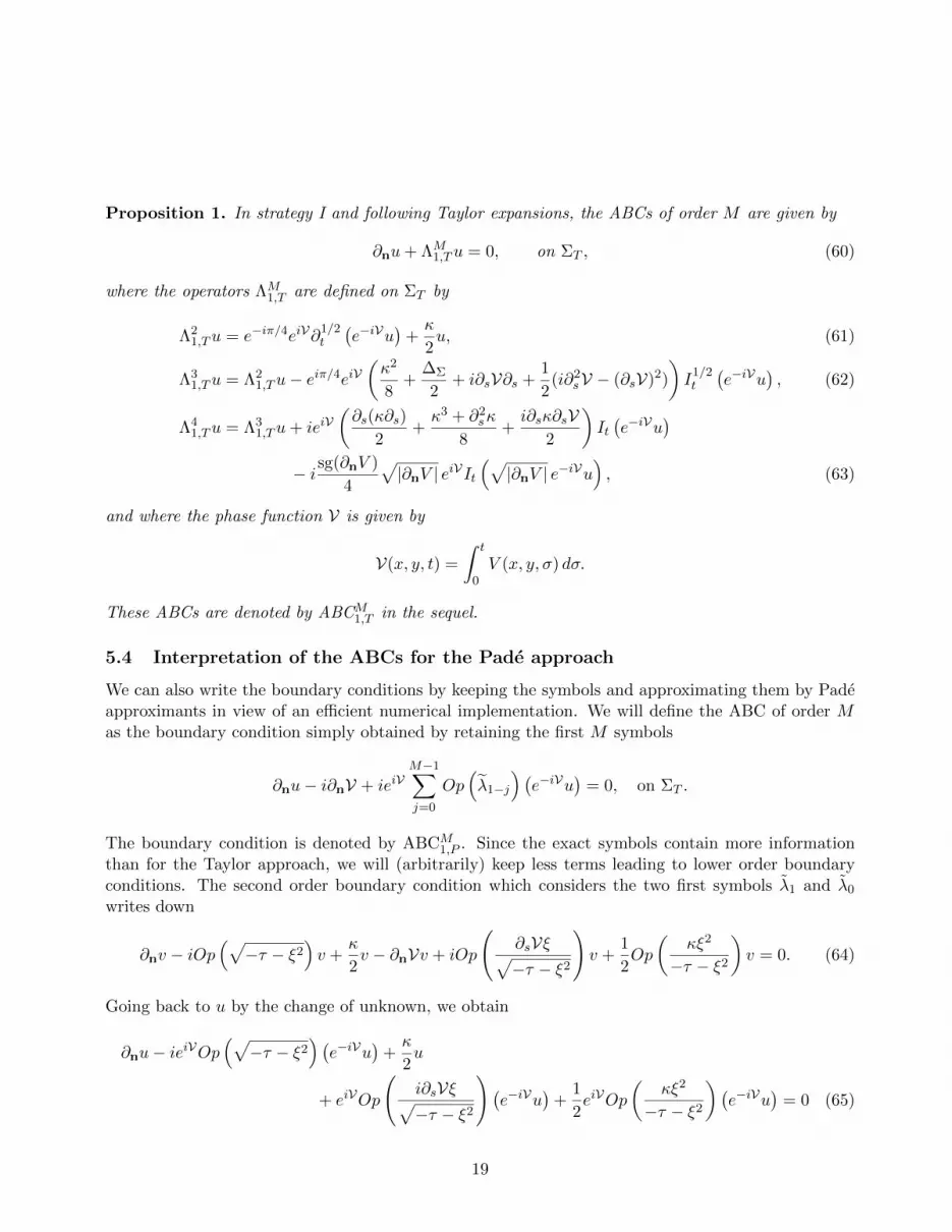
Proposition 1. In strategy I and following Taylor expansions, the ABCs of order M are given by

∂nu+ ΛM1,Tu = 0, on ΣT , (60)

where the operators ΛM1,T are defined on ΣT by

Λ21,Tu = e−iπ/4eiV∂

1/2t

(e−iVu

)+κ

2u, (61)

Λ31,Tu = Λ2

1,Tu− eiπ/4eiV(κ2

8+

∆Σ

2+ i∂sV∂s +

1

2(i∂2

sV − (∂sV)2)

)I

1/2t

(e−iVu

), (62)

Λ41,Tu = Λ3

1,Tu+ ieiV(∂s(κ∂s)

2+κ3 + ∂2

sκ

8+i∂sκ∂sV

2

)It(e−iVu

)− isg(∂nV )

4

√|∂nV | eiVIt

(√|∂nV | e−iVu

), (63)

and where the phase function V is given by

V(x, y, t) =

∫ t

0V (x, y, σ) dσ.

These ABCs are denoted by ABCM1,T in the sequel.

5.4 Interpretation of the ABCs for the Pade approach

We can also write the boundary conditions by keeping the symbols and approximating them by Padeapproximants in view of an efficient numerical implementation. We will define the ABC of order Mas the boundary condition simply obtained by retaining the first M symbols

∂nu− i∂nV + ieiVM−1∑j=0

Op(λ1−j

) (e−iVu

)= 0, on ΣT .

The boundary condition is denoted by ABCM1,P . Since the exact symbols contain more information

than for the Taylor approach, we will (arbitrarily) keep less terms leading to lower order boundaryconditions. The second order boundary condition which considers the two first symbols λ1 and λ0

writes down

∂nv − iOp(√−τ − ξ2

)v +

κ

2v − ∂nVv + iOp

(∂sVξ√−τ − ξ2

)v +

1

2Op

(κξ2

−τ − ξ2

)v = 0. (64)

Going back to u by the change of unknown, we obtain

∂nu− ieiVOp(√−τ − ξ2

) (e−iVu

)+κ

2u

+ eiVOp

(i∂sVξ√−τ − ξ2

)(e−iVu

)+

1

2eiVOp

(κξ2

−τ − ξ2

)(e−iVu

)= 0 (65)

19

We have the following link between the symbols and the operators

Op(√−τ − ξ2

)=√i∂t + ∆Σ,

Op

(iξ√−τ − ξ2

)= ∂s (i∂t + ∆Σ)−1/2 = (i∂t + ∆Σ)−1/2 ∂s,

Op

(ξ2

−τ − ξ2

)= −∆Σ (i∂t + ∆Σ)−1 = − (i∂t + ∆Σ)−1 ∆Σ. (66)

Here, since the operators to identify are independent of s and t, these substitutions are exact unlikewhat we will observe in the second strategy. Hence, we have the second order boundary condition

∂nu− ieiV√i∂t + ∆Σ

(e−iVu

)+κ

2u+ ∂sVeiV∂s (i∂t + ∆Σ)−1/2 (e−iVu)

− κ

2eiV (i∂t + ∆Σ)−1 ∆Σ

(e−iVu

)= 0. (67)

The first order boundary condition is deduced by truncation. We do not give the higher order boundaryconditions which would not be useful for computational purpose. The following proposition summa-rizes the results.

Proposition 2. For strategy I and following a Pade approximation, the ABCs of order M are givenby

∂nu+ ΛM1,Pu = 0, on ΣT (68)

where the operators ΛM1,P are defined on ΣT by

Λ11,Pu = −ieiV

√i∂t + ∆Σ

(e−iVu

), (69)

Λ21,Pu = Λ1

1,Pu+κ

2u+ ∂sVeiV∂s (i∂t + ∆Σ)−1/2 (e−iVu)− κ

2eiV (i∂t + ∆Σ)−1 ∆Σ

(e−iVu

). (70)

We specify these boundary conditions by ABCM1,P .

Remark 3. Looking at (66), two equivalent interpretations are possible for λ+−2: ∆Σ (i∂t + ∆Σ)−1

or (i∂t + ∆Σ)−1 ∆Σ. We choose the second solution for implementation issues in a finite elementframework [6].

6 Strategy II: direct method

In this strategy, we directly work on the equation (8) and we must solve the equation in λ+ given by(39)

i∂rλ+ + iκrλ

+ ++∞∑|α|=0

(−i)|α|

α!∂α(ξ,τ)λ

+∂α(t,r)λ+ = −τ − h−2ξ2 + ih−1(∂sh

−1)ξ + Vr. (71)

20

6.1 Computation of the symbols

Let us begin by fixing the principal symbol. This can be achieved by extracting the second orderterms in (71). Like the gauge change, we must determine which second order terms in the right handside of (71) must be retained. The direct method consists in including the potential in the principalsymbol to compensate the gauge change effect. We exclude the case λ+

1 = ±√−τ − h−2ξ2 (which

corresponds to the zero order strategy in Remark 1 leading to less accurate ABCs). Considering theterm ih−1∂sh

−1ξ is excluded since we have no sign control. Finally, the principal symbol is

λ+1 = ∓

√−τ − h−2ξ2 + Vr. (72)

The sign of λ+1 is chosen to fix the outgoing wave. The term −τ − h−2ξ2 + Vr is real valued and its

square-root is a complex number with a null or positive imaginary part. Therefore, the minus signmust be considered to get a negative imaginary part for λ+

1 . The principal symbol is then

λ+1 = −

√−τ − h−2ξ2 + Vr. (73)

The computation of λ+0 is obtained by considering the first order terms in (71). These are solutions

toi∂rλ

+1 + iκrλ

+1 + 2λ+

1 λ+0 = ih−1(∂sh

−1)ξ.

However, since λ+1 is non homogeneous, ∂rλ

+1 is the sum of two terms with different homogeneities,

respectively 1 and −1,

∂rλ+1 =

∂r(h−1)ξ2

2√−τ − h−2ξ2 + Vr

− ∂rVr

2√−τ − h−2ξ2 + Vr

.

We use the notation:(∂rλ

+1

)1

to designate the part of ∂rλ+1 which is of order 1, and similarly for the

order −1. With these notations, the equation for the first order terms writes

i(∂rλ

+1

)1

+ iκrλ+1 + 2λ+

1 λ+0 = ih−1(∂sh

−1)ξ.

The term of order −1(∂rλ

+1

)−1

will be considered when the terms of order −1 will be collected in the

computation of λ+−2. Hence, all the terms of each equation must be carefully studied to know their

correct order. Finally, we have

λ+0 = − i

2κr +

i

4

(∂rh−2)ξ2

−τ − h−2ξ2 + ih−1(∂sh−1)ξ + Vr− i

4

h−2(∂sh−2)ξ3√

−τ − h−2ξ2 + ih−1(∂sh−1)ξ + Vr3 .

We also compute λ+−1 and λ+

−2 which are next evaluated at r = 0 to get the associated operators Λ+.

21

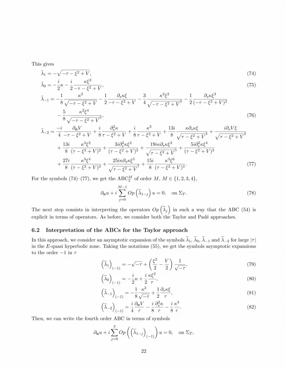
This gives

λ1 = −√−τ − ξ2 + V , (74)

λ0 = − i2κ− i

2

κξ2

−τ − ξ2 + V, (75)

λ−1 = −1

8

κ2√−τ − ξ2 + V

− 1

2

∂sκξ

−τ − ξ2 + V− 3

4

κ2ξ2√−τ − ξ2 + V

3 −1

2

∂sκξ3

(−τ − ξ2 + V )2

− 5

8

κ2ξ4√−τ − ξ2 + V

5 , (76)

λ−2 =−i4

∂nV

−τ − ξ2 + V+i

8

∂2sκ

τ − ξ2 + V+i

8

κ3

τ − ξ2 + V+

13i

8

κ∂sκξ√τ − ξ2 + V

3 +i∂sV ξ√

τ − ξ2 + V3

+13i

8

κ3ξ2

(τ − ξ2 + V )2+

3i∂2sκξ

2

(τ − ξ2 + V )2+

19iκ∂sκξ3√

τ − ξ2 + V5 +

5i∂2sκξ

4

(τ − ξ2 + V )3

+27i

8

κ3ξ4

(τ − ξ2 + V )3+

25iκ∂sκξ5√

τ − ξ2 + V7 +

15i

8

κ3ξ6

(τ − ξ2 + V )4. (77)

For the symbols (74)–(77), we get the ABCM2 of order M , M ∈ 1, 2, 3, 4,

∂nu+ i

M−1∑j=0

Op(λ1−j

)u = 0, on ΣT . (78)

The next step consists in interpreting the operators Op(λj

)in such a way that the ABC (54) is

explicit in terms of operators. As before, we consider both the Taylor and Pade approaches.

6.2 Interpretation of the ABCs for the Taylor approach

In this approach, we consider an asymptotic expansion of the symbols λ1, λ0, λ−1 and λ−2 for large |τ |in the E-quasi hyperbolic zone. Taking the notations (55), we get the symbols asymptotic expansionsto the order −1 in τ (

λ1

)(−1)

= −√−τ +

(ξ2

2− V

2

)1√−τ

, (79)(λ0

)(−1)

= − i2κ+

i

2

κξ2

τ, (80)(

λ−1

)(−1)

= −1

8

κ2

√−τ

+1

2

∂sκξ

τ, (81)(

λ−2

)(−1)

=i

4

∂nV

τ− i

8

∂2sκ

τ− i

8

κ3

τ. (82)

Then, we can write the fourth order ABC in terms of symbols

∂nu+ i

3∑j=0

Op

((λ1−j

)(−1)

)u = 0, on ΣT ,

22

which gives

∂nu+ e−iπ/4∂1/2t u+

κ

2u− eiπ/4

(κ2

8+

∆Σ

2+V

2

)I

1/2t u

+ i

(∂s(κ∂s)

2+κ3

8+∂2sκ

8− ∂nV

4

)Itu = 0

Like for the gauge change method, we try to obtain a symmetrical ABC to get a priori estimates. We

symmetrize the two termsV

2and

∂nV

4, by writing

V = sg(V )√|V |√|V |

and∂nV = sg(∂nV )

√|∂nV |

√|∂nV |

The resulting ABC is denoted by ABC42,T . We directly have some lower order ABCs. The result is

embedded in the following proposition.

Proposition 3. In strategy II (direct method) and by using a Taylor expansion, the ABCs of orderM are given by

∂nu+ ΛM2,Tu = 0, on ΣT , (83)

where the operators ΛM2,T are defined on ΣT by

Λ12,Tu = e−iπ/4∂

1/2t u, (84)

Λ22,Tu = Λ1

2,Tu+κ

2u, (85)

Λ32,Tu = Λ2

2,Tu− eiπ/4(κ2

8+

∆Σ

2

)I

1/2t u− eiπ/4 sg(V )

2

√|V | I1/2

t

(√|V |u

), (86)

Λ42,Tu = Λ3

2,Tu+ i

(∂s(κ∂s)

2+κ3 + ∂2

sκ

8

)It u− i

sg(∂nV )

4

√|∂nV | It

(√|∂nV |u

). (87)

The boundary conditions are denoted by ABCM2,T in the sequel.

Remark 4. Let us note the symmetrical form of Λ32,T and Λ4

2,T . We also obtain here the ABCs expectedfrom strategy zero (see subsection 4.2, Remark 1). This shows that strategy II is more general.

6.3 Interpretation of the ABCs and Pade approach

For the Pade approach, the first order ABC is obtained by retaining the first symbol λ1

∂nu− iOp(√−τ − ξ2 + V

)u = 0 (88)

and the second order ABC by adding λ0

∂nu− iOp(√−τ − ξ2 + V

)u+

κ

2u+

1

2Op

(κξ2

−τ − ξ2 + V

)u = 0. (89)

Since we consider the symbols globally, we retain less terms in the expansion. For implementationissues, it is necessary to interpret the operators. We use the following approximations.

23

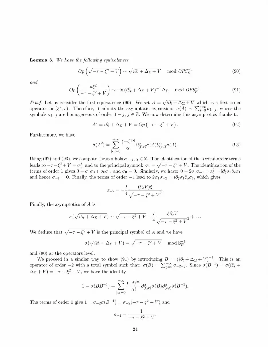
Lemma 3. We have the following equivalences

Op(√−τ − ξ2 + V

)∼√i∂t + ∆Σ + V mod OPS−1

E (90)

and

Op

(κξ2

−τ − ξ2 + V

)∼ −κ (i∂t + ∆Σ + V )−1 ∆Σ mod OPS−3

E . (91)

Proof. Let us consider the first equivalence (90). We set A =√i∂t + ∆Σ + V which is a first order

operator in (ξ2, τ). Therefore, it admits the asymptotic expansion: σ(A) ∼∑+∞

j=0 σ1−j , where thesymbols σ1−j are homogeneous of order 1− j, j ∈ Z. We now determine this asymptotics thanks to

A2 = i∂t + ∆Σ + V = Op(−τ − ξ2 + V

). (92)

Furthermore, we have

σ(A2) =+∞∑|α|=0

(−i)|α|

α!∂α(ξ,τ)σ(A)∂α(s,t)σ(A). (93)

Using (92) and (93), we compute the symbols σ1−j , j ∈ Z. The identification of the second order terms

leads to −τ−ξ2 +V = σ21, and to the principal symbol: σ1 =

√−τ − ξ2 + V . The identification of the

terms of order 1 gives 0 = σ1σ0 + σ0σ1, and σ0 = 0. Similarly, we have: 0 = 2σ1σ−1 + σ20 − i∂ξσ1∂sσ1

and hence σ−1 = 0. Finally, the terms of order −1 lead to 2σ1σ−2 = i∂ξσ1∂sσ1, which gives

σ−2 = − i4

(∂sV )ξ√−τ − ξ2 + V

3 .

Finally, the asymptotics of A is

σ(√i∂t + ∆Σ + V ) ∼

√−τ − ξ2 + V − i

4

ξ∂sV√−τ − ξ2 + V

3 + . . .

We deduce that√−τ − ξ2 + V is the principal symbol of A and we have

σ(√i∂t + ∆Σ + V ) =

√−τ − ξ2 + V mod S−1

E

and (90) at the operators level.We proceed in a similar way to show (91) by introducing B = (i∂t + ∆Σ + V )−1. This is an

operator of order −2 with a total symbol such that: σ(B) =∑+∞

j=0 σ−2−j . Since σ(B−1) = σ(i∂t +

∆Σ + V ) = −τ − ξ2 + V , we have the identity

1 = σ(BB−1) =+∞∑|α|=0

(−i)|α|

α!∂α(ξ,τ)σ(B)∂α(s,t)σ(B−1).

The terms of order 0 give 1 = σ−2σ(B−1) = σ−2(−τ − ξ2 + V ) and

σ−2 =1

−τ − ξ2 + V.

24

We next obtain the equations 0 = σ−3σ(B−1) and σ−3 = 0, then 0 = σ−4σ(B−1), and σ−4 = 0.Finally, the terms of order −3 lead to σ−5σ(B−1) = i∂ξσ−2∂sσ(B−1), and

σ−5 =2i∂sV ξ

(−τ − ξ2 + V )3.

We deduce the asymptotics of the inverse operator

σ(

(i∂t + ∆Σ + V )−1)∼ 1

−τ − ξ2 + V+

2i∂sV ξ

(−τ − ξ2 + V )3+ . . . .

We can now compute the asymptotics of −κ (i∂t + ∆Σ + V )−1 ∆Σ. Function κ is independent of ξand τ , and so

σ(−κ (i∂t + ∆Σ + V )−1 ∆Σ

)= −κσ

((i∂t + ∆Σ + V )−1 ∆Σ

).

By the composition formula, we can write that

−κσ(

(i∂t + ∆Σ + V )−1 ∆Σ

)= − κ

+∞∑|α|=0

(−i)|α|

α!∂α(ξ,τ)σ

((i∂t + ∆Σ + V )−1

)∂α(s,t)σ (∆Σ)

= κ ξ2 σ(

(i∂t + ∆Σ + V )−1)

since all the terms are equal to zero for |α| ≥ 1. Hence, we have

σ(−κ (i∂t + ∆Σ + V )−1 ∆Σ

)∼ κ ξ2

−τ − ξ2 + V+

2iκ∂sV ξ3

(−τ − ξ2 + V )3+ . . . .

The symbolκξ2

−τ − ξ2 + Vcan finally be interpreted as the principal symbol of−κ (i∂t + ∆Σ + V )−1 ∆Σ,

leading to (91).

From Lemma 3, we deduce ABCs for strategy II that we denote by ABCM2,P , and which are given

in Proposition 4.

Proposition 4. In strategy II and following a Pade approach, the ABCs of order M are given by

∂nu+ ΛM2,Pu = 0, on ΣT , (94)

where the operators ΛM2,P are defined on ΣT by

Λ12,Pu = −i

√i∂t + ∆Σ + V u, (95)

Λ22,Pu = Λ2

2,Pu+κ

2u− κ

2(i∂t + ∆Σ + V )−1 ∆Σu. (96)

The ABCs are denoted by ABCM2,P .

Remark 5. We saw in paragraph 3.2 that for a time independent radial potential we have the corre-spondence between the gauge change and direct methods. It can be proved that this is the case forthe ABCs ABCM

1,P and ABCM2,P by using the Pade approach while not for the Taylor approach where

the symmetry is broken.

25

7 A priori estimates

7.1 Principle

We have four families of ABCs related to Strategy I and II, Taylor or Pade approximation. TheseABCs are given in Propositions 1, 2, 3 and 4 for ABCM

1,T , ABCM1,P , ABCM

2,T and ABCM2,P , respectively.

In [7], for the free-potential equation, ABCs have been built and correspond to strategy II with Taylorapproximation for V = 0. For these ABCs, we have the following result [7].

Proposition 5. Let u0 ∈ L2(Ω) and u solution to(i∂t + ∆u) = 0, in Ω× R+∗,

∂nu+ TMu = 0, on Σ× R+∗,

u(x, 0) = u0(x), in Ω,

(97)

where the operators TM are defined on Σ× R+∗ by

T 1u = e−iπ/4∂1/2t u, T 2u = T 1u+

κ

2u,

T 3u = T 2u− eiπ/4(κ2

8+

∆Σ

2

)I

1/2t u,

T 4u = T 3u+ i

(κ3

8+

1

2∂s(κ∂s) +

∂2sκ

8

)Itu.

Then, u is unique and defined in C([0;T ], L2(Ω)

). Moreover, u satisfies the energy inequality

∀t ∈ [0;T ], ‖u(t)‖L2(Ω) ≤ ‖u0‖L2(Ω). (98)

The idea is to generalize this Proposition to the ABCs with potential, that is ABCM1,T or ABCM

2,T .

For ΛM1,T and ΛM2,T , this seems pretty simple to generalize Proposition 5 to Λ21,T because of the symmetry

of the operators. This is however more difficult for Λ31,T (and Λ4

1,T ) since we have no sign control on

i∂2sV − (∂sV)2.

For the second strategy, the operators are closer to TM since there is no change of variable. Theinteresting point is to analyze if the added terms modify or not the result. For Λ1

2,T = T 1 and

Λ22,T = T 2, the result is direct since it does not include any potential term. The operators Λ3

2,T and

Λ42,T are respectively modified by terms V and ∂nV compared to T 3 and T 4. Our study will mainly

analyze these two additional terms. We will need the following Lemma [9].

Lemma 4. Let ϕ ∈ H1/4([0; t], L2(Σ)

)and ψ ∈ L2

([0; t], L2(Σ)

)that we extend to zero on R \ [0; t].

Then we have ∫R×Σ

ϕ(s, t′) ∂1/2t′ ϕ(s, t′)dt′dΣ ∈ eiπ/4R+ ∪ e−iπ/4R+, (99)∫

R×Σψ(s, t′) I

1/2t′ ψ(s, t′)dt′dΣ ∈ eiπ/4R+ ∪ e−iπ/4R+, (100)∫

R×Σψ(s, t′) It′ψ(s, t′)dt′dΣ ∈ iR. (101)

26

Proof. Let τ and ξ be respectively the Fourier covariables of t′ and s and let u be the Fourier transformof u. Let us first remark that for a general pseudodifferential operator P (s, t′, ξ, τ) with symbolp(s, t′, ξ, τ), we have the identity∫

R×Σϕ(s, t′)P (s, t′, ∂s, ∂t)ϕ(s, t′) dt′dΣ =

∫R×R

p(s, t′, ξ, τ)|ϕ(ξ, τ)|2dτdξ. (102)

Indeed, Plancherel’s Theorem implies that∫R×Σ

ϕ(s, t′)Pϕ(s, t′) dt′dΣ =

∫R×R

F (ϕ)(ξ, τ)F(P ϕ(s, t′)

)(ξ, τ) dτdξ.

But, from the definition of the symbol of an operator, we have

F(P ϕ(s, t′)

)(ξ, τ) = σ (P ) ϕ(ξ, τ) = p(s, t′, ξ, τ)ϕ(ξ, τ),

and so (102)∫R×Σ

ϕ(s, t′)Pϕ(s, t′) dt′dΣ =

∫R×R

ϕ(ξ, τ)p(s, t′, ξ, τ)ϕ(ξ, τ) dt′dΣ =

∫R×R

p(s, t′, ξ, τ)|ϕ(ξ, τ)|2dτdξ.

We next apply this result to ∂1/2t′ with symbol

√iτ . We must determine the part of the complex plane in

which this symbol lies. For positive τ we have√iτ = eiπ/4

√τ , and for negative τ ,

√iτ = e−iπ/4

√−τ ,

leading to the expected property (99). A very similar proof gives the result for I1/2t′ et It′ with

respective symbols σ(I1/2t′ ) = 1√

iτand σ (It′) = 1

iτ .

Lemma 4 is the basic ingredient to derive a priori estimates for ABCM1,T and ABCM

2,T .

Remark 6. The Pade based ABCs will not be considered here. We cannot apply our proof and moredevelopments should be considered.

7.2 A priori estimates for ABCM2,T

Concerning the family of ABCs ABCM2,T , the following result holds.

Theorem 2. Let u0 ∈ L2(Ω) an initial data with compact support in Ω. Let V ∈ C∞(R2 ×R+,R) bea real-valued potential. We denote by u a solution to the initial boundary value problem

i∂tu+ ∆u+ V u = 0, in ΩT ,

∂nu+ ΛM2,Tu = 0, on ΣT ,

u(x, 0) = u0(x), in Ω

(103)

where the operators ΛM2,T , M ∈ 1, 2, 3, 4, are defined in Proposition 3. Then, u satisfies the inequality

∀t > 0, ‖u(t)‖L2(Ω) ≤ ‖u0‖L2(Ω) (104)

for M = 1 and M = 2. Moreover, this inequality is also satisfied for M = 3 under the assumptionthat V is positive on Σ, and for M = 4 under the hypothesis that sg(∂nV ) is constant over Σ for anytime. In particular, this implies the uniqueness of the solution u of the initial boundary value problem(103).

27

Proof. Let T ∈]0;T ]. Let us introduce x = (x, y) ∈ R2. We begin by extending u to a function udefined over R in the following way

u(·, t) =

u(·, t) for t ∈ [0; T ]

0 for t ∈]−∞; 0[∪]T ; +∞[.

In the distributions sense, we obtain

∂tu(x, t) =

∂tu(x, t)− u(x, T )δT (t) + u0(x)δ0(t), t ∈ [0; T ]

0, t ∈]−∞; 0[∪]T ; +∞[

∆u(x, t) =

∆u(x, t), t ∈ [0; T ]

0, t ∈]−∞; 0[∪]T ; +∞[

∂nu+ ΛM2,T u = 0.

The function u satisfies the equation

i∂tu+ ∆u+ V u = −iu(x, T )δT + iu0(x)δ0(t), on Ω× R

Multiplying this equation by −iu(x, t), we get

u∂tu− iu∆u− iuV u = −u(x, T )uδT (t) + u0(x)uδ0(t).

We integrate by part over Ω∫Ωu∂tu dΩ− i

∫Σu ∂nu dΣ + i

∫Ω|∇u|2dΩ− i

∫ΩV |u|2dΩ

= −∫

Ωu(x, T )u δT (t)dΩ +

∫Ωu0(x)u δ0(t)dΩ (105)

and next take the real part of this expression by assuming that V is a real-valued potential∫Ω∂t|u|2

2dΩ− Re

(i

∫Σ∂nuu dΣ

)= −Re

(∫Ωu(x, T )uδT (t)dΩ

)+ Re

(∫Ωu0(x)uδ0(t)dΩ

)(106)

We integrate on t ∈ R. The terms in the left hand side give∫R

∫Ωu(x, T )u(x, t)δT (t)dΩdt =

∫Ωu(x, T )

∫Ru(x, t)δT (t)dtdΩ =

∫Ωu(x, T )u(x, T )dΩ = ‖u(T )‖2L2(Ω)

since u(x, T ) = u(x, T ), and∫R

∫Ωu0(x)u(x, t)δ0(t)dΩdt =

∫Ωu0(x)u(x, 0) dΩ = ‖u0‖2L2(Ω),

because u(x, 0) = u(x, 0) = u0(x). Furthermore, since u is zero at ±∞, we have∫Ω

∫R∂t|u|2

2dtdΩ =

∫Ω

[|u(x, t)|2

2

]+∞

−∞= 0.

28

Finally, after a time integration of (106), we obtain

Re

(i

∫Σ×R

u ∂nu dΣdt

)= ‖u(T )‖2L2(Ω) − ‖u0‖2L2(Ω) (107)

for any T ∈ [0;T ], and where ∂nu is given by the chosen boundary condition. For the sake ofconciseness, we note u instead of u, having in mind that u is equal to zero outside [0; T ].

Let us first begin by ABC22,T given by the operator (85). We have to analyze the sign of the real

part of the two following terms∫Σ×R

iu ∂nu dΣdt = −ie−iπ/4∫

Σ×Ru ∂

1/2t u dΣdt− i

2

∫Σ×R

κ |u|2 dΣdt. (108)

To this end we use the identity (102). We have

−ie−iπ/4∫

Σ×Ru ∂

1/2t u dΣdt = −ie−iπ/4

∫R×R|u(ξ, τ)|2σ(∂

1/2t )dξdτ.

However, σ(∂1/2t ) =

√iτ which varies in e−iπ/4R+ ∪ eiπ/4R+ for τ in R, implies that the real part

of (108) is negative. Since the second term is purely imaginary, (104) is proved for the second orderABC.

We consider now the fourth order ABC ABC42,T given by the operator (87). The boundary condition

can be decomposed in seven terms Aj , 1 ≤ j ≤ 7, as follows∫Σ×R

iu∂nu dΣdt =

∫Σ×R

(−ie−iπ/4u∂1/2

t u+ ieiπ/4u∆Σ

2I

1/2t u

)dΣdt− i

2

∫Σ×R

κ |u|2 dΣdt

+ ieiπ/4∫

Σ×R

κ2

8u I

1/2t u dΣdt+ ieiπ/4

∫Σ×R

sg(V )

2

√|V |u I1/2

t

(√|V |u

)dΣdt

− 1

2

∫Σ×R

u ∂s(κ∂s)Itu dtΣdt+

∫Σ×R

κ3 + ∂2sκ

8u Itu dΣdt

−∫

Σ×R

sg(∂nV )

4

√|∂nV |u It

(√|∂nV |u

)dΣdt

=7∑j=1

Aj .

(109)Therefore, we have to study the sign of the real part of each term. We use several times the identity(102). We have

A1 =

∫R×R|u(ξ, τ)|2σ

(−ie−iπ/4∂1/2

t + ieiπ/4∆Σ

2I

1/2t

)dξdτ.

Furthermore, we also can write that

a1(ξ, τ) := σ

(−ie−iπ/4∂1/2

t + ieiπ/4∆Σ

2I

1/2t

)=−i2

(2e−iπ/4

√iτ + eiπ/4

ξ2

√iτ

).

29

For τ > 0, we have√iτ = eiπ/4

√τ and so

a1(ξ, τ) =−i2

(2√τ +

ξ2

√τ

).

The symbol a1(ξ, τ) is then a pure imaginary number in this case. For τ < 0, we write√iτ =

e−iπ/4√−τ and we have

a1(ξ, τ) =−i2

(−2i√−τ + i

ξ2

√−τ

)= −√−τ +

1

2

ξ2

√−τ

=1

2√−τ

(τ + τ + ξ2

).

However, we work in the E-quasi hyperbolic zone H in which τ + ξ2 < 0. As a consequence, thereal number a1(ξ, τ) satisfies a1(ξ, τ) < τ

2√−τ < 0 and its real part is negative. Finally, we have

Re(A1) ≤ 0. The term A2 is purely imaginary. The term A3 fulfills

A3 = ieiπ/4∫R×R|u(ξ, τ)|2a3(ξ, τ)dξdτ,

where

a3(ξ, τ) = σ

(κ2

8I

1/2t

)=κ2

8

1√iτ

∈ eiπ/4R+ ∪ e−iπ/4R+.

We deduce that A3 varies in R− ∪ iR+ and so has a real negative part. Since we assume that Vremains positive over Σ, and then sg(V ) is equal to 1, we can write A4 by applying the Plancherel’sidentity in time

A4 = ieiπ/4∫

Σ

1

2

∫R

√|V |u I1/2

t

(√|V |u

)dtdΣ,

= ieiπ/4∫

Σ

1

2

∫R

∣∣∣Ft(√|V |u)

∣∣∣2 (s, τ)1√iτdτdΣ.

Here, we apply Lemma 4 but only working on the time integral and taking the time Fourier transform.The integral over τ varies in eiπ/4R+ ∪ e−iπ/4R+, and so A4 ∈ R− ∪ iR+ and A4 has a negative realpart.

The next three additional terms are related to the fourth order ABC. Under the assumption on∂nV , we show that they are all purely imaginary. The first one, A5, is treated by a integration bypart over the closed curve Σ and by using the commutativity of It and ∂s∫

Σu ∂s(κ∂sItu) dΣ = −

∫Σ∂suκ∂sItu dΣ = −

∫Σ∂suκ It(∂su) dΣ

and then

A5 =1

2

∫Σ×R

∂suκIt (∂su) dΣdt =1

2

∫R×R

∣∣∣∂su(ξ, τ)∣∣∣2 κ

iτdξdτ.

Since κ is a real number, the term A5 is a pure imaginary number. The term A6 is also purelyimaginary since

A6 =

∫R×R|u(ξ, τ)|2κ

3 + ∂2sκ

8

1

iτdξdτ.

30

Finally, for A7 we consider the time integral

A7 = −∫

Σ

sg(∂nV )

4

∫R

√|∂nV |u It

(√|∂nV |u

)dtdΣ

= −∫

Σ

sg(∂nV )

4

∫R

∣∣∣Ft(√|∂nV |u)(s, τ)

∣∣∣2 1

iτdτdΣ

which is purely imaginary. Finally, we have

Re

(i

∫Σ×R

u ∂nu dΣdt

)≤ 0,

and then, for any time T ∈ [0;T ], ‖u(T )‖L2(Ω) ≤ ‖u0‖L2(Ω), ending hence the proof for M = 4.To get the result for the third order ABC, we do not consider A5, A6 and A7.

7.3 A priori estimates for ABCM1,T

We have the following results for the family of ABCs ABCM1,T .

Theorem 3. Let u0 ∈ L2(Ω) an initial data with compact support in Ω. Let V ∈ C∞(R2 ×R+,R) bea real-valued potential. We denote by u a solution to the initial boundary value problem

i∂tu+ ∆u+ V u = 0, in ΩT ,

∂nu+ ΛM1,Tu = 0, on ΣT ,

u(x, 0) = u0(x), in Ω

(110)

where the operators ΛM1,T , M ∈ 2, 3, 4 are defined in Proposition 1. Then, u satisfies the energyinequality

∀t > 0, ‖u(t)‖L2(Ω) ≤ ‖u0‖L2(Ω) (111)

for M = 2. Furthermore, if V a a radial potential: V (r, s, t) = V (r, t), then the energy inequality(111) is also satisfied for M = 3 and M = 4 if we assume that sg(∂nV ) is time independent over Σ.In particular, this implies the uniqueness of the solution u of the initial boundary value problem (110).

Proof. We first consider the second-order boundary condition for a general potential V (r, s, t). Thebeginning of the proof is the same as in Theorem 3, until the equality (107). We consider now theboundary condition ABC2

1,T given by the operator (61). We get∫Σ×R

iu∂nu dΣdt = −ie−iπ/4∫

Σ×ReiVu ∂

1/2t

(e−iVu

)dΣdt− i

2

∫Σ×R

κ|u|2dΣdt. (112)

The second term is clearly purely imaginary. The first term can be written as

−ie−iπ/4∫

Σ×ReiVu ∂

1/2t

(e−iVu

)dΣdt = −ie−iπ/4

∫R×R

∣∣F(s,t)(e−iVu)(ξ, τ)

∣∣2√iτ dξdτand so varies in R− ∪ iR−, which ends the proof for M = 2.

31

Let us assume now that V = V (r, t) is a radial potential. Then the phase function V is also radial.The operator Λ2

1,T remains unchanged but since ∂sV = 0, the operators Λ31,T and Λ4

1,T respectivelywrite down

Λ31,Tu = Λ2

1,Tu− eiπ/4eiV(κ2

8+

∆Σ

2

)I

1/2t

(e−iVu

),

Λ41,Tu = Λ3

1,Tu+ ieiV(∂s(κ∂s)

2+κ3 + ∂2

sκ

8

)It(e−iVu

)− i

4sg(∂nV )

√|∂nV | eiVIt

(√|∂nV | e−iVu

),

by using the symmetric form of Λ41,T . The third order boundary condition considers the additional

terms∫Σ×R

iu∂nu dΣdt =

∫Σ×R

(−ie−iπ/4eiVu ∂1/2

t

(e−iVu

)+ ieiπ/4eiVu

∆Σ

2I

1/2t

(e−iVu

))dΣdt

− i

2

∫Σ×R

κ|u|2dΣdt+ ieiπ/4∫

Σ×R

κ2

8eiVu I

1/2t

(e−iVu

)dΣdt.

(113)

The first term can be treated in a similar way as ABCM2,T and the second one is purely imaginary.

Finally, the third term is analyzed as before. Then, we only obtain some terms with a negative or nullreal part for the third order ABC. Let us now consider the fourth order ABC for radial potentials.We must study the sign of the additional terms

−∫

Σ×R

1

2eiVu ∂s(κ∂s)It

(e−iVu

)dΣdt−

∫Σ×R

eiVuκ3 + ∂2

sκ

8It(e−iVu

)dΣdt

+

∫Σ×R

1

4sg(∂nV )eiV

√|∂nV |u It

(e−iV

√|∂nV |u

)dΣdt

(114)

These three terms can be treated as for ABC42,T : the first one by integration by part over Σ, and next

applying the identity (102) after using the assumption over sg(∂nV ) which is time independent. Thisends the proof for M = 4.

Remark 7. Let us remark that the results cannot be extended to M ≥ 3 when the potential is notradial. Indeed, we then have to study the sign of the real part of the terms

−eiπ/4∫R×R

∣∣F (e−iVu)(ξ, τ)∣∣2 (∂sV)

iξ√iτdξdτ

and

ieiπ/4∫R×R

∣∣F (e−iVu)(ξ, τ)∣∣2 (i∂2

sV − (∂sV)2)1√iτdξdτ.

However, the symbol (∂sV) iξ√iτ

varies in eiπ/4R ∪ e−iπ/4R without restricting the lines to half-lines

studies since ξ describes R and has no fixed sign. Consequently the first integral takes values in R× iRand its real part may be either positive or negative. The same problem arises for the second integral(i∂2

sV − (∂sV)2) which is complex. Therefore, estimates can only be obtained for radial potentials forABCs of order 3 or higher in which case these two integrals vanish.

32

8 Conclusion

We proposed the construction of absorbing boundary conditions for the two-dimensional Schrodingerequation with a general potential and for a curved convex fictitious boundary. We essentially obtainedfour families of ABCs according to strategy I (gauge change) or II (direct method), with a Taylorexpansion or a Pade approach. The discretization schemes of these ABCs will be introduced andanalyzed in a forthcoming paper [6]. Furthermore, numerical examples will show how these ABCscompare.

References

[1] X. Antoine, A. Arnold, C. Besse, M. Ehrhardt, and A. Schadle. A review of transparent and ar-tificial boundary conditions techniques for linear and nonlinear Schrodinger equations. Commun.Comput. Phys., 4(4):729–796, 2008.

[2] X. Antoine, H. Barucq, and A. Bendali. Bayliss-Turkel-like radiation conditions on surfaces ofarbitrary shape. J. Math. Anal. Appl., 229(1):184–211, 1999.

[3] X. Antoine and C. Besse. Construction, structure and asymptotic approximations of a microd-ifferential transparent boundary condition for the linear Schrodinger equation. J. Math. PuresAppl. (9), 80(7):701–738, 2001.

[4] X. Antoine and C. Besse. Unconditionally stable discretization schemes of non-reflecting boundaryconditions for the one-dimensional Schrodinger equation. J. Comput. Phys., 188(1):157–175, 2003.

[5] X. Antoine, C. Besse, and P. Klein. Absorbing boundary conditions for the one-dimensionalSchrodinger equation with an exterior repulsive potential. J. Comput. Phys., 228(2):312–335,2009.

[6] X. Antoine, C. Besse, and P. Klein. Absorbing boundary conditions for the two-dimensionalSchrodinger equation with an exterior potential. Part II: Discretization and numerical results. inpreparation, 2011.

[7] X. Antoine, C. Besse, and V. Mouysset. Numerical schemes for the simulation of the two-dimensional Schrodinger equation using non-reflecting boundary conditions. Math. Comp.,73(248):1779–1799 (electronic), 2004.

[8] X. Antoine, C. Besse, and J. Szeftel. Towards accurate artificial boundary conditions for nonlinearPDEs through examples. Cubo, 11(4):29–48, 2009.

[9] N. Ben Abdallah, F. Mehats, and O. Pinaud. On an open transient Schrodinger-Poisson system.Math. Models Methods Appl. Sci., 15(5):667–688, 2005.

[10] J.-P. Berenger. A perfectly matched layer for the absorption of electromagnetic waves. J. Comput.Phys., 114(2):185–200, 1994.

[11] A. Boutet de Monvel, A. S. Fokas, and D. Shepelsky. Analysis of the global relation for thenonlinear Schrodinger equation on the half-line. Lett. Math. Phys., 65(3):199–212, 2003.

33

[12] R. Carles. Linear vs. nonlinear effects for nonlinear Schrodinger equations with potential. Com-mun. Contemp. Math., 7(4):483–508, 2005.

[13] T. Cazenave. An introduction to nonlinear Schrodinger equations. Instituto de Matematica-UFRJ,Rio de Janeiro, RJ, 1996.

[14] P. Debernardi and P. Fasano. Quantum confined Stark effect in semiconductor quantum wellsincluding valence band mixing and Coulomb effects. IEEE Journal of Quantum Electronics,29:2741–2755, 1993.

[15] A. del Campo, G. Garcia-Calderon, and J. G. Muga. Quantum transients. Physics Report-ReviewSection of Physics Letters, 476(1-3):1–50, May 2009.

[16] B. Engquist and A. Majda. Absorbing boundary conditions for the numerical simulation of waves.Math. Comp., 31(139):629–651, 1977.

[17] B. Engquist and A. Majda. Radiation boundary conditions for acoustic and elastic wave calcula-tions. Comm. Pure Appl. Math., 32(3):313–357, 1979.

[18] R. Lascar. Propagation des singularites des solutions d’equations pseudo-differentielles quasihomogenes. Ann. Inst. Fourier (Grenoble), 27(2):vii–viii, 79–123, 1977.

[19] M. Levy. Non-local boundary conditions for radiowave propagation. Phys. Rev. E, 62(1):1382–1389, Jul 2000.

[20] M. Levy. Parabolic equation methods for electromagnetic wave propagation, volume 45 of IEEElectromagnetic Waves Series. Institution of Electrical Engineers (IEE), London, 2000.

[21] E. Lorin, A. Bandrauk, and S. Chelkowski. Numerical Maxwell-Schrodinger model for laser-molecule interaction and propagation. Comput. Phys. Comm., 177 (12):908–932, 2007.

[22] E. Lorin, A. Bandrauk, and S. Chelkowski. Mathematical modeling of boundary conditionsfor laser-molecule time dependent Schrodinger equations and some aspects of their numericalcomputation-One-dimensional case. Numer. Meth. for P.D.E., 25:110–136, 2009.

[23] J. G. Muga, J. P. Palao, B. Navarro, and I. L. Egusquiza. Complex absorbing potentials. Phys.Rep., 395(6):357–426, 2004.

[24] L. Nirenberg. Pseudodifferential operators and some applications, volume 17 of Regional Conf.Ser. in Math. AMS 17, Lectures on Linear Partial Differential Equations. AMS, 1973.

[25] J. Szeftel. Design of absorbing boundary conditions for Schrodinger equations in Rd. SIAM J.Numer. Anal., 42(4):1527–1551 (electronic), 2004.

[26] J. Szeftel. Absorbing boundary conditions for one-dimensional nonlinear Schrodinger equations.Numer. Math., 104(1):103–127, 2006.

[27] O. Vacus. Mathematical analysis of absorbing boundary conditions for the wave equation: Thecorner problem. Math. Comp., 74(249):177–200, 2004.

34

[28] C. Zheng. A perfectly matched layer approach to the nonlinear Schrodinger wave equations. J.Comput. Phys., 227(1):537–556, 2007.

[29] C. Zheng. An exact absorbing boundary condition for the Schrodinger equation with sinusoidalpotentials at infinity. Commun. Comput. Phys., 3(3):641–658, 2008.

35