arX

iv:0

909.

0468

v1 [

cond

-mat

.sof

t] 2

Sep

200

9

Anomalous phase behavior of a soft-repulsive potential

with a strictly monotonic force

Franz Saija1 [†], Santi Prestipino2 [‡] and Gianpietro Malescio2 [*]

1 CNR-Istituto per i Processi Chimico-Fisici,

Contrada Papardo, 98158 Messina, Italy

2 Universita degli Studi di Messina, Dipartimento di Fisica,

Contrada Papardo, 98166 Messina, Italy

(Dated: June 12, 2013)

Abstract

We study the phase behavior of a classical system of particles interacting through a strictly

convex soft-repulsive potential which, at variance with the pairwise softened repulsions considered

so far in the literature, lacks a region of downward or zero curvature. Nonetheless, such interaction

is characterized by two length scales, owing to the presence of a range of interparticle distances

where the repulsive force increases, for decreasing distance, much more slowly than in the adjacent

regions. We investigate, using extensive Monte Carlo simulations combined with accurate free-

energy calculations, the phase diagram of the system under consideration. We find that the model

exhibits a fluid-solid coexistence line with multiple re-entrant regions, an extremely rich solid

polymorphism with solid-solid transitions, and water-like anomalies. In spite of the isotropic nature

of the interparticle potential, we find that, among the crystal structures in which the system can

exist, there are also a number of non-Bravais lattices, such as cI16 and diamond.

PACS numbers: 61.20.Ja, 62.50.-p, 64.70.D-

Keywords: Soft-core potentials, High-pressure phase diagram of the elements, Liquid-solid transitions, Solid-

solid transitions, Reentrant melting, Water-like anomalies

1

I. INTRODUCTION

In typical models of effective pairwise interaction between particles, the repulsive force

steadily increases, with an ever-increasing rate, as particles get more and more closer to

each other. This behavior, which is typical of e.g. the Lennard-Jones potential, is originated

by the harsh quantum repulsion that is associated with the overlapping of electronic shells.

However, effective classical interactions where the repulsive component undergoes some form

of softening in a range of interparticle distances are relevant for many physical systems. Most

of them belong to the realm of so-called soft matter (solutions of star polymers, colloidal

dispersions, microgels, etc.) [1, 2], but also the adiabatic interaction potential (electronic in

origin) of simple atomic systems under high pressure is manifestly of the soft-core type [3, 4].

The effects of particle-core softening on thermodynamic behavior were first investigated

by Hemmer and Stell [5], who analysed the possible occurrence of multiple critical points

and isostructural solid-solid transitions. These authors considered pair potentials with a

hard core augmented with a finite repulsive component in the form of a square shoulder

or a linear ramp, features that may be pertinent to some pure metallic systems, metallic

mixtures, electrolytes, and colloidal systems. Few years later, Young and Alder [6] showed

that the hard core plus square shoulder potential gives origin to an anomalous melting

line similar to that observed in Cs or Ce. Later, Debenedetti [7] showed that systems of

particles interacting via potentials whose repulsive core is softened by a curvature change are

capable of contracting when heated isobarically (a behavior known as “density anomaly”).

More recently, intense investigation of the phase behavior of potentials with a softened

core has shown that these models can yield, even for isotropic one-component systems,

unusual properties such as a melting line with a maximum followed by a region of re-entrant

melting, polymorphism both in the fluid and solid phases, and a rich hierarchy of water-like

anomalies [8, 9, 10, 11, 12, 13, 14, 15, 16, 17, 18, 19, 20].

The common feature of all the softened-core potentials investigated so far is that, in a

range of interparticle distances r, the strength of the two-body force f(r) ≡ −u′(r) reduces

or at most remains constant as two particles approach each other, u(r) being the repulsive

part of the pair potential. In this interval of distances, u(r) shows a downward or zero

concavity, i.e., u′′(r) ≤ 0. Assuming that the repulsion is hard-core-like at small distances

and goes to zero sufficiently fast at large distances, the above behavior makes it possible to

2

identify two distinct regions where the repulsive force increases as r gets smaller: a inner

region, associated with the impenetrable particle core, and an outer region at large distances.

Such potentials are thus endowed with two repulsive length scales: a smaller one (“hard”

radius), which is dominant at the higher pressures, and a larger one (“soft” radius), being

effective at low pressure. In the range of pressures where the two length scales compete,

a system governed by soft-core interactions behaves as a “two-state” system, a simplified

viewpoint that nonetheless provides an explanation for re-entrant melting and, in presence

of an additional attractive long-range force, for the existence of a liquid-liquid transition [21].

Though core-softening has been usually associated to a repulsive force with non-

monotonic behavior, the latter condition might be an unnecessary requirement. This obser-

vation stems from an analysis of the mathematical expression of core-softening, which was

put forward by Debenedetti et al. [7] under the form: ∆(rf(r)) < 0 for ∆r < 0, in some

interval r1 < r < r2, together with u′′(r) > 0 for r < r1 and r > r2. The above conditions

are satisfied if, in the interval (r1, r2), the product rf(r) (rather than just f) reduces with

decreasing interparticle separation. Hence, the core-softening property may also be satisfied

with a strictly convex potential, yielding a repulsive force which everywhere increases for

decreasing r, provided that, in a range of interparticle distances, the increasing rate of f(r)

be sufficiently small. On this basis, we expect that the class of core-softened potentials is in

fact much wider than thought before.

We hereafter study the phase diagram of a model potential which is soft, according to

Debenedetti’s formulation, though being characterized by a strictly monotonic force for all

distances (i.e., u′′(r) > 0 everywhere). We find that this potential exhibits the whole spec-

trum of anomalies that are usually associated with soft-core potentials, including re-entrant

melting regions, solid polymorphism, and water-like anomalies. This paper is organized as

follows: in Sec. 2, we describe the model system which is the subject of our investigation. In

Sec. 3, we outline the simulation method that is used to map out the phase diagram. The

simulation results are presented and discussed in Sec. 4 while further remarks and conclusions

are postponed to Sec. 5.

3

II. MODEL

We consider a purely repulsive pair potential modelled through an exponential form, first

introduced, about four decades ago, by Yoshida and Kamakura (YK) [22]:

u(r) = ǫ exp

{

a(

1 −r

σ

)

− 6(

1 −r

σ

)2

ln( r

σ

)

}

, (1)

where ǫ and σ are the energy and length units respectively and a > 0. This potential

behaves as r−6 for small r, and falls off very rapidly for large r. The softness of the repulsion

is controlled by the a parameter. When a < 1.9, the YK potential has a region with

downward curvature where the force decreases as two particles get closer.

Approximate theoretical calculations [22] suggest that the melting line of the YK potential

might display a re-entrant melting region for values of a that are larger than 1.9, i.e., even

when no downward concavity is present. In order to explore this possibility and discuss it

in relation with other anomalous behaviors, we have investigated the phase behavior of the

YK potential for a = 2.1 through numerical simulation. For this a value (as well as for all

a’s falling in the range 1.9−2.3) u(r) is strictly convex (see Fig. 1), i.e., its second derivative

is positive everywhere, hence the repulsive force is strictly increasing for decreasing r, at

variance with the core-softened potentials considered so far. However, the rate at which the

force increases is not monotonous. By the way, in a range of r that roughly corresponds to

the local minimum of u′′(r), the repulsive force increases with decreasing r much more slowly

than in the adjacent regions, in such a way that the Debenedetti core-softening property is

still satisfied.

III. METHOD

A major problem, when drawing the phase diagram of a model system of particles inter-

acting through an assigned potential, is to identify the solid phases. This is a critical issue

for soft-core repulsions since experience has shown that many different crystal structures

are stabilized for such systems upon varying the pressure [4, 16, 19, 23]. In the present

study, we consider as candidates for the solid phase precisely those crystal structures that

a previous investigation of the same potential [4] showed to be stable at zero temperature.

These include the face-centered cubic (fcc), body-centered cubic (bcc), and simple hexagonal

(sh) lattices, as well as a number of non-Bravais lattices, i.e., the A7, diamond, A20, and

4

hexagonal close-packed (hcp) lattices. On increasing pressure, each of these structures gives,

in turn, the most stable structure at T = 0. The sequence of stable crystals for increasing

pressures was found to be [4]:

fcc0.63−→ bcc

1.26−→ sh

2.29−→ A7

2.55−→ diamond

4.91−→ sh

5.46−→ A20

12.07−→ hcp

15.68−→ bcc

52.75−→ fcc

138.28−→ hcp

365.65−→ fcc ,

(2)

where the numbers above the arrows indicate the transition pressures expressed, to within

a precision of 0.01, in units of ǫ/σ3. Where pertinent, the values of the internal parameters

of the phases listed in Eq. 2 are reported in Ref. [4]. Although the above sequence of phases

resulted from a careful scrutiny of about thirty crystal structures, we cannot exclude that

some relevant structure might have been overlooked. In general, we may expect that the

same crystals that are stable at T = 0 also give the underlying lattice structure for the solid

phases at T > 0. Anyway, if more crystals exist at T = 0 with nearly the same chemical

potential µ in a pressure range, each of them represents a potentially relevant solid phase.

In our case, this occurs for P ≈ 2.4, where the ground state is of A7 type but some oC8

and cI16 crystals have only slightly larger chemical potentials. Hence, we include also these

lattices in our list of solid candidates.

We calculate the phase diagram of the YK model for a = 2.1 by performing Monte Carlo

(MC) simulations in the isothermal-isobaric, NPT ensemble (i.e., at constant temperature

T , pressure P and number N of particles), as well as in the canonical, NV T ensemble, using

the standard Metropolis algorithm with periodic boundary conditions and the nearest-image

convention. In the solid phases, the number of particles is chosen so as to guarantee a

negligible contribution to the interaction energy from pairs of particles separated by half the

minimum simulation-box length. With this choice, we checked in a number of cases that the

exact location of phase boundaries is only negligibly affected by the finite size of the sample.

More precisely, our samples consisted of 500 particles in the fcc phase, of 432 particles in the

bcc phase, of 800 particles in the sh phase, of 512 particles in the diamond phase, of 1024

particles in the cI16 phase, of 1152 particles in the A7 phase, and of 768 particles in the oC8

phase. Depending on the solid phase with which the fluid is compared to in order to assess

its relative stability, we consider fluid samples of 500 to 800 particles. At given T and P ,

sample equilibration typically took from 20000 to 50000 MC sweeps, a sweep consisting of

one average attempt per particle to change its position plus (for the NPT case only) one

5

attempt to change the volume through a rescaling of particle coordinates. The maximum

random displacement of a particle and the maximum volume change in a trial MC move

are adjusted every sweep during the equilibration run so as to obtain an acceptance ratio of

moves close to 50% (afterwards, during the production session, they are maintained fixed).

Thermodynamic averages are computed over trajectories from 3 × 104 to 105 sweeps long.

In a typical NPT simulation, we generate a sequence of simulation runs along an isobar,

starting from the cold solid on one side and from the hot fluid on the other side (a chain

of NV T runs along an isotherm at a sufficiently high temperature provides the link to a

dilute-fluid state). The last configuration produced in a given run is taken to be the first

of the next run at a slightly different temperature. The starting configuration of a “solid”

chain of runs is a low-temperature perfect crystal whose density is set equal to its T = 0

value at that pressure. In case of a structure with internal parameters, the same T = 0

optimal parameters are chosen in the preparation of the crystal sample. Usually, a series of

runs is continued until a sudden change is found in the difference of energy/volume between

the solid and the fluid, so as to avoid averaging over heterogeneous thermodynamic states.

The density of a solid phase ordinarily varies very little with increasing temperature along

an isobar. A sudden density change thus indicates a mechanic instability of the solid in

favour of the fluid, hence it signals the approximate location of melting. In fact, this so

called “heat-until-it-melts” (HUIM) procedure allows to locate the maximum overheating

temperature T ′

m, which may however be substantially higher than the fluid-solid coexistence

temperature Tm.

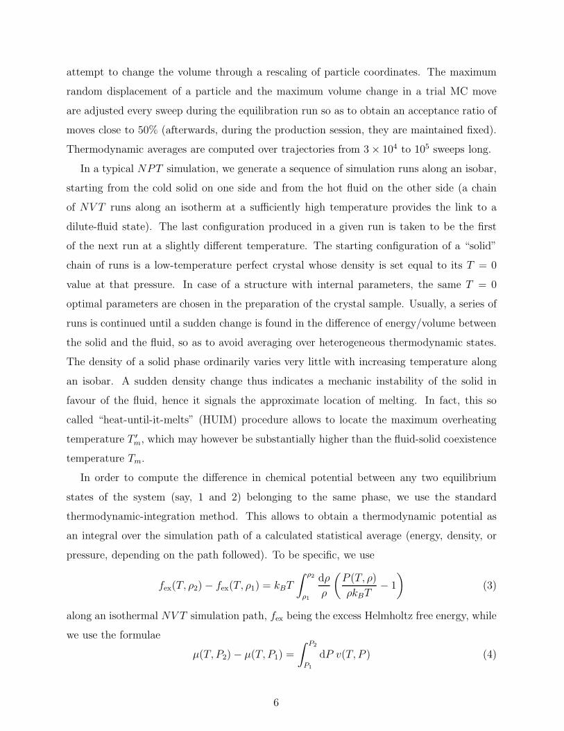
In order to compute the difference in chemical potential between any two equilibrium

states of the system (say, 1 and 2) belonging to the same phase, we use the standard

thermodynamic-integration method. This allows to obtain a thermodynamic potential as

an integral over the simulation path of a calculated statistical average (energy, density, or

pressure, depending on the path followed). To be specific, we use

fex(T, ρ2) − fex(T, ρ1) = kBT

∫ ρ2

ρ1

dρ

ρ

(

P (T, ρ)

ρkBT− 1

)

(3)

along an isothermal NV T simulation path, fex being the excess Helmholtz free energy, while

we use the formulae

µ(T, P2) − µ(T, P1) =

∫ P2

P1

dP v(T, P ) (4)

6

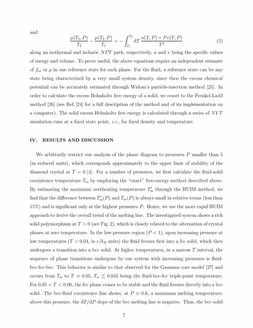
andµ(T2, P )

T2

−µ(T1, P )

T1

= −

∫ T2

T1

dTu(T, P ) + Pv(T, P )

T 2(5)

along an isothermal and isobaric NPT path, respectively, u and v being the specific values

of energy and volume. To prove useful, the above equations require an independent estimate

of fex or µ in one reference state for each phase. For the fluid, a reference state can be any

state being characterized by a very small system density, since then the excess chemical

potential can be accurately estimated through Widom’s particle-insertion method [25]. In

order to calculate the excess Helmholtz free energy of a solid, we resort to the Frenkel-Ladd

method [26] (see Ref. [24] for a full description of the method and of its implementation on

a computer). The solid excess Helmholtz free energy is calculated through a series of NV T

simulation runs at a fixed state point, i.e., for fixed density and temperature.

IV. RESULTS AND DISCUSSION

We arbitrarily restrict our analysis of the phase diagram to pressures P smaller than 5

(in reduced units), which corresponds approximately to the upper limit of stability of the

diamond crystal at T = 0 [4]. For a number of pressures, we first calculate the fluid-solid

coexistence temperature Tm by employing the “exact” free-energy method described above.

By estimating the maximum overheating temperature T ′

m through the HUIM method, we

find that the difference between T ′

m(P ) and Tm(P ) is always small in relative terms (less than

15%) and is significant only at the highest pressures P . Hence, we use the more rapid HUIM

approach to derive the overall trend of the melting line. The investigated system shows a rich

solid polymorphism at T > 0 (see Fig. 2), which is closely related to the alternation of crystal

phases at zero temperature. In the low-pressure region (P < 1), upon increasing pressure at

low temperatures (T < 0.04, in ǫ/kB units) the fluid freezes first into a fcc solid, which then

undergoes a transition into a bcc solid. At higher temperatures, in a narrow T interval, the

sequence of phase transitions undergone by our system with increasing pressures is fluid-

bcc-fcc-bcc. This behavior is similar to that observed for the Gaussian core model [27] and

occurs from Ttr to T ≃ 0.05, Ttr . 0.045 being the fluid-bcc-fcc triple-point temperature.

For 0.05 < T < 0.06, the fcc phase ceases to be stable and the fluid freezes directly into a bcc

solid. The bcc-fluid coexistence line shows, at P ≃ 0.6, a maximum melting temperature;

above this pressure, the dT/dP slope of the bcc melting line is negative. Thus, the bcc solid

7

undergoes, for not too low temperatures, re-entrant melting into a denser fluid.

At low temperatures, the bcc solid transforms, for pressures around 1.3, into a solid

with a sh structure. Hence, there should be a fluid-bcc-sh triple point which terminates

the bcc reentrant melting line. This is illustrated in detail in Fig. 3, where we show the

calculated chemical potentials of the three phases along the T = 0.03 isotherm. Upon

further increasing pressure, a cI16 solid with internal parameter x = 0.125 becomes stable

(see Ref. [4] for a definition of x). This can occur only for high enough T since, in the

pressure interval 2.30 < P < 2.55, a certain A7 crystal has a lower chemical potential than

cI16 at T = 0 (we have checked that no oC8 solid is stable in the same temperature range).

In other words, a small A7 basin exists below T ≈ 0.01. Following the cI16 phase, another

solid phase arranged according to the diamond structure becomes stable in a broad pressure

range, starting from P ≃ 2.6.

Within the precision of our calculation, the overall melting line exhibits, in addition to

the first (bcc-fluid) re-entrant region, other portions with negative dT/dP slope, though

less pronounced than the first. The alternation of solid phases at low temperatures goes

on beyond P = 5 until, eventually, the system sets in a fcc solid that coexists with the

fluid phase at arbitrary high temperatures, the coexistence line becoming asymptotically

the same as for the r−6 potential. The complex phase behavior shown in Fig. 2 is absent in

the theoretical calculation of Yoshida et al. [22], where only the possibility of a fcc solid was

taken into account. With this limitation, only one region of reentrant melting is predicted

and the high-pressure fluid can be stable even at zero temperature. Moreover, the height and

width of the low-density solid region are largely overestimated by the theory as compared

to the simulation results here presented.

Our results show that the model system here considered, though described by a

spherically-symmetric potential, can exist under the form of stable non-Bravais crystals.

The rich polymorphism observed follows from the peculiar dependence of the interatomic

force with distance, which leads to the existence of two incommensurate length scales. In the

pressure and temperature regimes where these lengths compete with each other, compact ar-

rangements such as the fcc and bcc lattices are frustrated and low-coordinated arrangements

are preferred. Our results are relevant for those physical systems that are characterized by

a certain softness of the repulsive interaction. These include intrinsically soft materials such

as colloids, polymers, etc. but also atomic systems at extremely high pressures. Phase

8

diagrams with solid polymorphism and multiple re-entrant melting have been observed at

high pressures in some elements, such as Sr [29] and predicted by ab-initio simulation for

others [30]. Concerning model systems, a phase behavior with features similar to those

noted above was found for the hard-core plus repulsive step potential [16] and for Hertzian

spheres [19].

Some insight into the mechanisms that give origin to the complex phase behavior observed

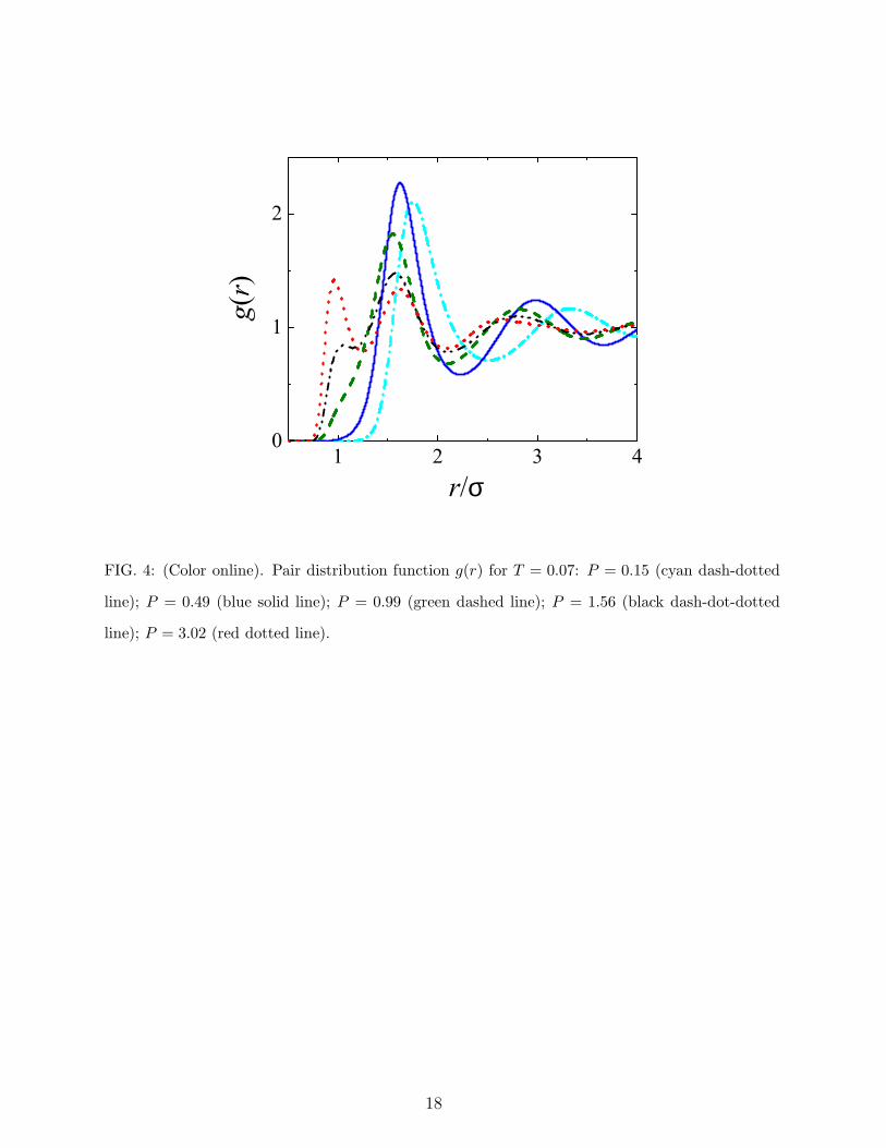
can be got from analysing the radial distribution function g(r). We computed g(r) for various

pressure values, at a temperature slightly larger than the maximum melting temperature

TM ≃ 0.06 of the bcc solid (Fig. 4). At very low pressure, the first peak of g(r) is centred

around r . 2 (in units of σ). As P increases up to P ≈ 0.50, this peak moves upward while

its position shifts towards r ≃ 1.5. For further pressure increase, its height decreases while

its position remains almost unaltered. At the same time, a new peak develops around r = 1,

whose height grows with P . This behavior is significantly different from that of simple fluids,

where all peaks of g(r) get higher with pressure when keeping T constant, and is consistent

with the gradual penetration of particles inside the inner core. Thus, the analysis of g(r)

points to the existence of two competitive scales of nearest-neighbour distance, i.e., a larger

soft length fading out with increasing pressure in favour of the smaller hard length. The

soft-repulsive distance falls approximately at r = 1.5, which is where the second derivative

of the potential has a local maximum, while the hard length scale remains defined by the

extremely rapid increase of the short-range repulsive force around r = 1.

Thermodynamic, dynamic and structural anomalies have been observed in a number of

substances (such as water, silica, silicon, carbon, and phosphorous) [21]. These unconven-

tional features are usually referred to as water-like anomalies. Although these substances

are all characterized by local tetrahedral order, in the last years water-like anomalies have

been found also in systems with spherically symmetric potentials, provided that the repul-

sion is of the softened-core type [8, 9, 10, 11, 12, 13, 14, 15, 16, 17, 18, 19, 20] In order

to investigate the existence of anomalies in our system, we first analysed the behavior of

the number density in the fluid phase above the melting line. We find that in the region

lying approximately above the re-entrant portion of the bcc-fluid coexistence line, decreas-

ing temperature at constant pressure leads first to a density increase and then, contrary

to standard behavior, to a density decrease for further cooling (Fig. 5). The anomalous

behavior of the density can be interpreted in terms of the existence of two repulsive length

9

scales: as T reduces at constant pressure, the larger soft scale becomes favoured with respect

to the smaller hard one. Thus, compact local structures are less favoured than open ones,

which causes a decrease in the number of particles within a given volume. The P -T region

where the density behaves anomalously is bounded from the above by the locus of points

where the density attains its maximum value, i.e., by the temperature of density maximum

(TMD) line, while its lower bound is the limit of stability of the fluid phase, namely the

bcc-fluid coexistence line (see Fig. 2). Within the region of density anomaly, the system

expands upon cooling under fixed pressure. Consistently, the thermal expansion coefficient

αP = (1/V )(∂V/∂T )P is negative, vanishing along the TMD line (Fig. 5).

A series of studies have shown that thermodynamic (and dynamic) anomalies are strongly

correlated with anomalous trends in the structural order of the system [31]. A measure of

this quantity is provided by the pair entropy per particle,

s2 = −kB

2ρ

∫

d3r [g(r) ln g(r) − g(r) + 1] , (6)

which describes the contribution of two-body spatial correlations to the excess entropy of the

fluid [32]. For a completely uncorrelated system, g(r) = 1 and then s2 = 0. For systems with

long-range order, spatial correlations persist over large distances and s2 becomes large and

negative. Thus −s2 can be taken as an indicator of structural order. This parameter yields

information about the average relative spacing of the particles, i.e., it describes the tendency

of particle pairs to adopt preferential separations. In the investigated system, the structural

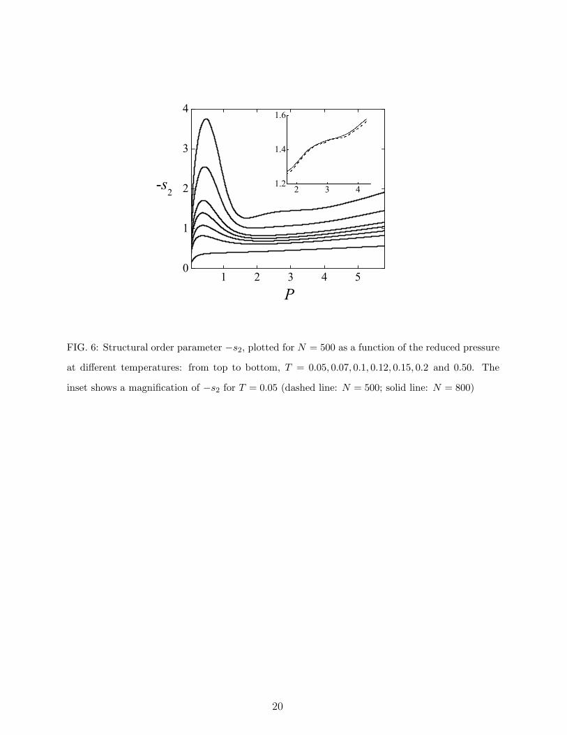
order initially increases upon compression (Fig. 6), similarly to simple fluids. However, as

pressure is further increased, −s2 attains a maximum value and then decreases, i.e., the fluid

loses structural order upon compression (structural anomaly). At sufficiently high density,

after attaining a local minimum, −s2 recovers a normal trend, increasing monotonously

with pressure. Upon increasing the temperature, the structural anomaly becomes less and

less marked (i.e., the difference between the local extrema of −s2 gets smaller). As seen

in Fig. 2, the region where the fluid has a structurally anomalous behavior embraces the

density anomaly region; a similar relationship between the structural and density anomalies

holds for water and for a number of model systems [31, 33, 34, 35].

Though, from a thermodynamic point of view, phase coexistence is determined solely by

the equality of the Gibbs free energy in the two phases, an incoming phase transition may in-

duce a number of modifications in the involved phases (the analysis of such changes provides

10

the basis for the so-called “one-phase” criteria for phase transitions). Here, we investigate

to what extent the rich solid polymorphism shown by our system at low temperature is re-

flected in the fluid lying at higher temperatures. The structural order, as measured by −s2,

offers interesting insight about this point. The behavior of −s2 shows that the low-density

bcc region casts an imprint on the surrounding fluid, under the form of a marked increase

of the structural order near the pressure of maximum melting temperature of the solid. On

the contrary, the detailed shape of the melting curve at intermediate densities does not sig-

nificantly affect the structural order of the fluid, which shows a steady enhancement with

pressure. In order to observe an appreciable modification of this behavior it is necessary to

examine the fluid very close to the solid. Only the lowest −s2 isotherm at T = 0.05, i.e., just

at the lower edge of the fluid phase, shows a modest bump reflecting the fine details of the

melting line (see Fig. 6). These results suggest that the influence of low-coordinated solid

structures on the structural order of the neighbouring fluid is much weaker than for compact

lattices. From the analysis of the g(r), it clearly appears that the soft-repulsive scale looses

efficacy in the pressure range corresponding approximately to the re-entrant region of the

bcc solid, where both density and structural anomalies occur. Beyond P = 1.5, the second

peak of g(r) changes only slightly (decreasing with increasing density), while the first peak

builds up significantly with pressure, which is the main reason for the steady increase of −s2

at intermediate pressures (this is related to the gradual increase of local order with compres-

sion, until the fluid crystallizes into a fcc structure at very high pressures, out of the range

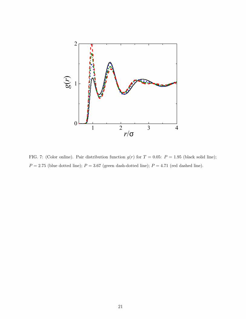
shown in Fig. 2). The third peak undergoes, with increasing pressure, subtle but significant

changes, splitting in two minor peaks (Fig. 7). Such changes mirror the alternation of the

solid structures at low T but, being small modifications of the g(r), they scarcely affect the

structural order of the fluid, at least that quantified by −s2.

V. CONCLUDING REMARKS

The occurrence of anomalous phase behavior within the class of isotropic one-component

classical potentials was, up to now, thought to be possible only for potentials with a region

of downward or zero curvature, where the repulsive force decreases or is at most constant as

two particles get closer. Here, we have shown that anomalous phase behaviors can actually

occur also for a system of particles interacting through a strictly monotonic repulsive force,

11

provided that in a range of interparticle distances the force increases more slowly, with

decreasing r, than in the adjacent regions. This condition gives origin, in spite of the

convexity of the potential, to two distinct repulsive length scales, a feature that seems

instrumental for the occurrence of re-entrant melting and the related water-like anomalies.

From the present results, we may expect that the real systems effectively characterized by

isotropic interactions and able to show unusual phase behaviors are more numerous than

previously believed.

12

[†] E-mail: saija@me.cnr.it (corresponding author)

[‡] E-mail: malescio@unime.it

[*] E-mail: Santi.Prestipino@unime.it

[1] C. N. Likos, Phys. Rep. 348, 267 (2001)

[2] C. N. Likos, Soft Matter 2, 478 (2006)

[3] G. Malescio, F. Saija, and S. Prestipino, J. Chem. Phys. 129, 241101 (2008)

[4] S. Prestipino, F. Saija, and G. Malescio, Soft Matter 5, 2795 (2009)

[5] P. C. Hemmer and G. Stell, Phys. Rev. Lett. 24, 1284 (1970)

[6] H. J. Young and B. J. Alder, Phys. Rev. Lett. 38, 1213 (1979); J. Chem. Phys. 70, 473 (1979)

[7] P. G. De Benedetti, V. S. Raghavan, and S. S. Borick, J. Phys. Chem. 95, 4540 (1991)

[8] F. H. Stillinger, J. Chem. Phys. 65, 3968 (1976)

[9] M. R. Sadr-Lahijany, A. Scala, S. Buldyrev, and H. E. Stanley, Phys. Rev. Lett. 81, 4895

(1998)

[10] E. A. Jagla, J. Chem. Phys. 111, 8980 (1999)

[11] P. Kumar, S. V. Buldyrev, F. Sciortino, E. Zaccarelli, H. E. Stanley, Phys. Rev. E 72, 021501

(2005)

[12] L. Xu, S. Buldyrev, C. A. Angell, and H. E. Stanley, J. Chem. Phys. 130, 054505 (2009)

[13] A. B. de Oliveira, P. A. Netz, T. Colla, and M. C. Barbosa, J. Chem. Phys. 124, 084505

(2006)

[14] H. M. Gibson and N. B. Wilding, Phys. Rev. E 73, 061507 (2006)

[15] E. Lomba, N. G. Almarza, C. Martin, C. McBridge, J. Chem. Phys. 126, 244510 (2006)

[16] D. Yu. Fomin, N. V. Gribova, V. N. Ryzhov, S. M. Stishov, D. Frenkel, J. Chem. Phys. 129,

064512 (2008)

[17] A. B. de Oliveira, G. Franzese, P. A. Netz, and M. C. Barbosa, J. Chem. Phys. 128, 064901

(2008)

[18] O. Pizio, H. Dominguez, Y. Duda, and S. Sokolowski, J. Chem. Phys. 130, 174504 (2009)

[19] J. C. Pamies, A. Cacciuto, and D. Frenkel, cond-mat/0811.2227

[20] G. J. Pauschenwein and G. Kahl, J. Chem. Phys. 129, 174107 (2008)

[21] P. F. McMillan, J. Mater. Chem. 14, 1506 (2004)

13

[22] T. Yoshida and S. Kamakura, Prog. Theor. Phys. 47, 1801 (1972); Prog. Theor. Phys. 52,

822 (1974); Prog. Theor. Phys. 56, 330 (1976); S. Kamakura and T. Yoshida, Prog. Theor.

Phys. 48, 2110 (1972)

[23] C. N. Likos, N. Hoffmann, H. Lowen, and A. A. Louis, J. Phys.: Condens. Matter 14, 7681

(2002)

[24] S. Prestipino and F. Saija, J. Chem. Phys. 126, 194902 (2007)

[25] B. Widom, J. Chem. Phys. 39, 2808 (1963)

[26] D. Frenkel and A. J. C. Ladd, J. Chem. Phys. 81, 3188 (1984); see also J. M. Polson, E.

Trizac, S. Pronk, and D. Frenkel, J. Chem. Phys. 112, 5339 (2000)

[27] S. Prestipino, F. Saija, and P. V. Giaquinta, Phys Rev. E 71, 050102 (2005)

[28] See e.g. F. Saija, S. Prestipino, and P. V. Giaquinta, J. Chem. Phys. 115, 7586 (2001)

[29] D. Errandonea, R. Boehler, and M. Ross, Phys. Rev. B 65 012108 (2001)

[30] A. A. Correa, S. A. Bonev, and G. Galli, Proc. Nat. Acad. Sci. USA 103, 1204 (2006)

[31] J. R. Errington and P. G. Debenedetti, Nature 409, 318 (2001)

[32] R. E. Nettleton and M. S. Green, J. Chem. Phys. 29, 1365 (1958)

[33] R. Esposito, F. Saija, A. M. Saitta, and P. V. Giaquinta, Phys. Rev. E 73, 040502 (2006)

[34] Z. Yan, S. V. Buldyrev, N. Giovambattista, and H. E. Stanley, Phys. Rev. Lett. 95, 130604

(2005)

[35] Z. Yan, S. V. Buldyrev, N. N. Giovambattista, P. G. Debenedetti, and H. E. Stanley, Phys.

Rev. E 73, 051204 (2006)

14

0.5 1.0 1.5 2.00

1

2

3

4

r/σ

FIG. 1: (Color online). Yoshida-Kamakura potential u(r) for a = 2.1 (black solid line, expressed in

ǫ units), two-body force f(r) = −u′(r) (blue dashed line, ǫ/σ units), product rf(r) (green dotted

line, ǫ units), second derivative of the potential u′′(r) (red dash-dotted line, ǫ/σ2 units)

15

0 1 2 3 4 50.00

0.05

0.10

0.15BA

diamond

A7

cI16shbccfcc

P

T

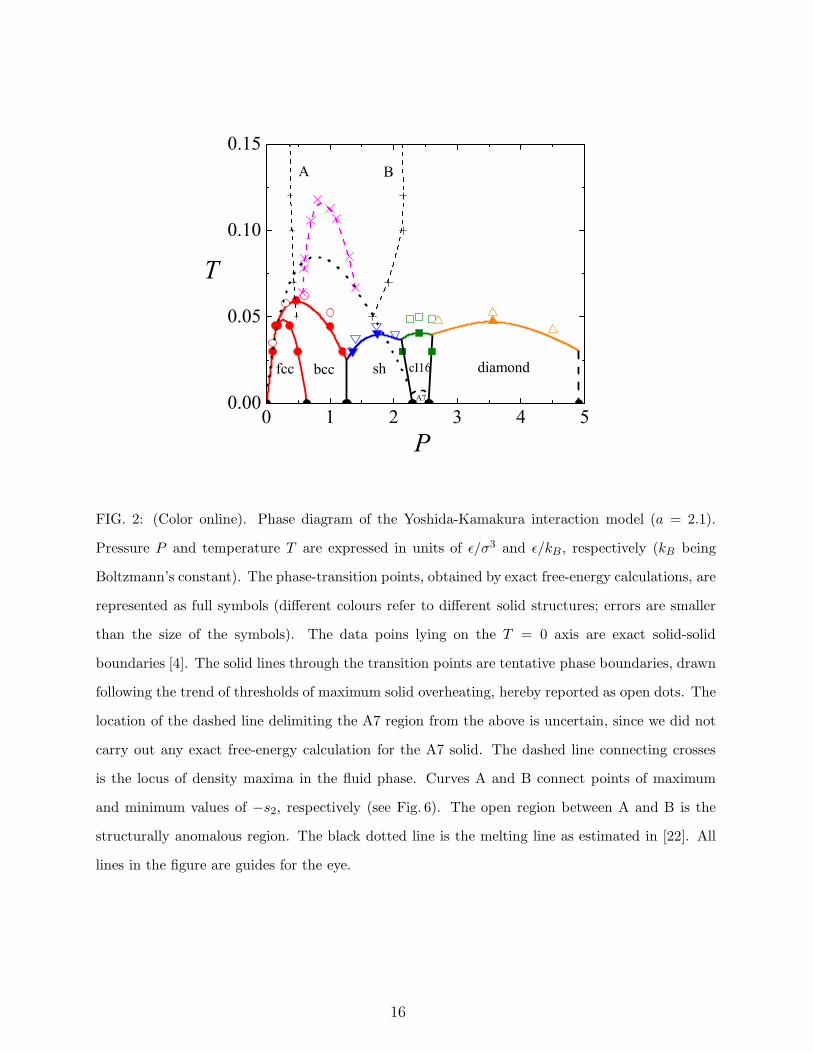
FIG. 2: (Color online). Phase diagram of the Yoshida-Kamakura interaction model (a = 2.1).

Pressure P and temperature T are expressed in units of ǫ/σ3 and ǫ/kB , respectively (kB being

Boltzmann’s constant). The phase-transition points, obtained by exact free-energy calculations, are

represented as full symbols (different colours refer to different solid structures; errors are smaller

than the size of the symbols). The data poins lying on the T = 0 axis are exact solid-solid

boundaries [4]. The solid lines through the transition points are tentative phase boundaries, drawn

following the trend of thresholds of maximum solid overheating, hereby reported as open dots. The

location of the dashed line delimiting the A7 region from the above is uncertain, since we did not

carry out any exact free-energy calculation for the A7 solid. The dashed line connecting crosses

is the locus of density maxima in the fluid phase. Curves A and B connect points of maximum

and minimum values of −s2, respectively (see Fig. 6). The open region between A and B is the

structurally anomalous region. The black dotted line is the melting line as estimated in [22]. All

lines in the figure are guides for the eye.

16

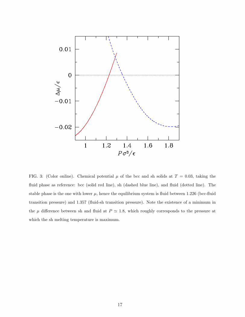
FIG. 3: (Color online). Chemical potential µ of the bcc and sh solids at T = 0.03, taking the

fluid phase as reference: bcc (solid red line), sh (dashed blue line), and fluid (dotted line). The

stable phase is the one with lower µ, hence the equilibrium system is fluid between 1.226 (bcc-fluid

transition pressure) and 1.357 (fluid-sh transition pressure). Note the existence of a minimum in

the µ difference between sh and fluid at P ≃ 1.8, which roughly corresponds to the pressure at

which the sh melting temperature is maximum.

17

1 2 3 40

1

2

g(r)

r/σ

FIG. 4: (Color online). Pair distribution function g(r) for T = 0.07: P = 0.15 (cyan dash-dotted

line); P = 0.49 (blue solid line); P = 0.99 (green dashed line); P = 1.56 (black dash-dot-dotted

line); P = 3.02 (red dotted line).

18

0.06 0.08 0.10 0.12 0.14 0.16-0.50

-0.25

0.00

T

α P

0.396

0.399

0.402

0.405

ρ

FIG. 5: Reduced number density ρ (upper panel) and thermal-expansion coefficient αP (lower

panel) plotted as a function of temperature for P = 1. The solid lines are polynomial fits of the

data. Note that αP vanishes approximately where ρ is maximum.

19

2 3 41.2

1.4

1.6

1 2 3 4 50

1

2

3

4

-s2

P

FIG. 6: Structural order parameter −s2, plotted for N = 500 as a function of the reduced pressure

at different temperatures: from top to bottom, T = 0.05, 0.07, 0.1, 0.12, 0.15, 0.2 and 0.50. The

inset shows a magnification of −s2 for T = 0.05 (dashed line: N = 500; solid line: N = 800)

20

1 2 3 40

1

2

g(r)

r/σ

FIG. 7: (Color online). Pair distribution function g(r) for T = 0.05: P = 1.95 (black solid line);

P = 2.75 (blue dotted line); P = 3.67 (green dash-dotted line); P = 4.71 (red dashed line).

21