81

AAS 07-104

THE MANY TRIAD ALGORITHMS*

Sergei Tanygin†

Malcolm D. Shuster‡

The different TRIAD algorithms are considered as specializations of the generalized TRIAD algorithm developed here. The attitude matrix estimate, error and covariance are developed for each algorithm. The optimal TRIAD algorithm is shown to be equivalent to first order to the optimal methods for solving Wahba’s problem for two vector observations.

INTRODUCTION

The simple and elegant TRIAD algorithm, invented by Harold D. Black in 1964 [1], was widely used in Spacecraft Attitude Estimation for nearly two decades. It was supplanted by the QUEST algorithm [2], which offered a way to process more than just two directional measurements and, based on them, produce optimal solutions to the Wahba problem [3]. Nevertheless, the TRIAD algorithm, because of its elegance and simplicity, has continued to be the object of research [2, 4-11].

Unlike the numerous solutions to the Wahba problem [12], which all minimize the same optimization criterion and are mathematically equivalent, the different varieties of the TRIAD algorithms offer different deterministic constructions for the attitude matrix and are guaranteed to be equivalent only for data uncorrupted by noise.

The earliest enhancement to the TRIAD algorithm was the symmetric TRIAD algorithm first reported by Lerner in 1978 [11]. In this algorithm, the usual inputs to the TRIAD algorithm are replaced by their unitized sum and difference. In 1981, it was shown that in the limit when the accuracy of the second direction becomes infinitely poorer compared to the first, the TRIAD algorithm yields the same attitude as the QUEST measurement model [2]. Since then, many additional connections between the TRIAD algorithm (or its symmetric variation) and the Wahba problem [3] for two measurements have been studied [5-7]. Several modifications of the TRIAD algorithm for the case of more than two measurements have also been examined [9, 13]. One of them, the suboptimal SCAD algorithm [13], restricted here to only two measurements is studied in this work under the name TRAD. The TRIAD algorithm has been expanded to treat attitude estimation in a Euclidean space of n dimensions, 3n > [4], and contracted to a Euclidean space of only two dimensions [8]. Recently, it has also been shown that in a limited sense, particularly for computing the attitude covariance matrix, the TRIAD algorithm can be treated as a maximum- likelihood estimator [10]. Even more recently new connections between the * F. Landis Markley has suggested that this work be retitled “Too Many TRIAD Algorithms.” † Sr. Astrodynamics Specialist, Analytical Graphics, Inc., 220 Valley Creek Blvd., Exton, PA 19341 email: stanygin@agi.com ‡ Director of Research, Acme Spacecraft Company, 13017 Wisteria Drive, Box 328, Germantown, Maryland 20874. email: mdshuster@comcast.net. website: http://home.comcast.net/~mdshuster.

82 Tanygin and Shuster

TRIAD algorithm and a solution to the Wahba problem [3] have been studied, namely, the possibility of finding the effective measurements for the Wahba problem which yield the same attitude estimate and attitude covariance matrix as the TRIAD algorithm [14], and the existence of a simple linear combination of the TRIAD algorithm for two orderings of the input directions which leads to an algorithm which is equivalent to a solution to the Wahba problem within the validity of the QUEST measurement model [15].

In the present work, we propose a generalization of the TRIAD algorithm (G-TRIAD) which establishes a framework within which we investigate the issue of optimality and examine multiple variations of the TRIAD algorithm as specializations of the G-TRIAD algorithm. These include:

• the basic TRIAD algorithm or TRIAD-I

• the reversed TRIAD algorithm or TRIAD-II

• the symmetric TRIAD algorithm (S-TRIAD)

• the TRAD algorithm

• the optimal TRIAD algorithm (O-TRIAD)

All of these variations simply modify the inputs to the basic TRIAD algorithm and are, therefore, very similar in execution. The TRAD and optimal TRIAD algorithms are presented for the first time in the present work.

In the present work, we generally follow the notation of Reference [16]. Specifically, we shall denote a random variable by the superscript “r.v.”, its realization by a prime and its true value by the superscript “true” (although we may omit the superscript entirely when the variable’s nature is clear from the context). The “ ∆ ” will, unless otherwise noted, always indicate a random infinitesimal quantity. An estimator (always a random variable) is usually denoted by an asterisk and an estimate by an additional prime.

THE ORIGINAL TRIAD ALGORITHM (TRIAD-I)

All variations of the TRIAD algorithm are constructed based on a pair of unit vectors represented in both the spacecraft body frame and the reference frame. The two vector observations in the body frame

1ˆ ′W and 2

ˆ ′W are the respective realizations of two random 3 ×1 column vectors r.v.1W and r.v.

2W with

respective true values true1W and true

2W . The corresponding vector representations in the reference frame

1V and 2V are considered to be always non-random and known (hence, always true values). These representations satisfy

r.v.1 1 1

ˆ ˆ ˆA= + ∆W V W and r.v.2 2 2

ˆ ˆ ˆA= + ∆W V W (1ab)

true1 1

ˆ ˆA=W V and true2 2

ˆ ˆA=W V (1cd)

with A the attitude matrix of the spacecraft body frame with respect to the reference frame.

The Many TRIAD Algorithms 83

All variations of the TRIAD algorithm also share the same basic idea for constructing the estimator of a (proper orthogonal) attitude matrix [1, 2]. They create the attitude matrix as a product of two proper orthogonal matrices one of which has columns defined by a right-hand orthonormal triad of column vectors constructed from the two vector observations and the other has its rows defined in the same manner but from the corresponding reference vectors. It is the differences in the manner of construction of right-hand orthonormal triads that give rise to the variety of TRIAD algorithms. In the original TRIAD algorithm, which has also been called the asymmetric TRIAD algorithm and the TRIAD-I algorithm [7], the two right-handed orthonormal triads { }r.v. r.v. r.v.

1 3 3ˆ ˆ ˆ, ,s s s and { }1 2 3ˆ ˆ ˆ, ,r r r are constructed

as follows

r.v. r.v. r.v.ˆ /i i i=s s s , ˆ /i i i=r r r , 1, 2,3i = (2ab)

with

r.v. r.v.1 1

ˆ=s W , r.v. r.v. r.v.2 1 2

ˆ ˆ= ×s W W , r.v. r.v. r.v.3 1 2= ×s s s (3abc)

1 1ˆ=r V , 2 1 2

ˆ ˆ= ×r V V , 3 1 2= ×r r r (4abc)

with the estimator defined as

TTRIAD* r.v. r.v. r.v.

1 2 3 1 2 3ˆ ˆ ˆ ˆ ˆ ˆA = s s s r r r (5)

where the superscript “T” denotes the matrix transpose. The related estimate and the true value of the attitude matrix are given by

TTRIAD*

1 2 3 1 2 3ˆ ˆ ˆ ˆ ˆ ˆA ′ ′ ′ ′= s s s r r r (6a)

and

( )true Ttrue TRIAD true true true1 2 3 1 2 3

ˆ ˆ ˆ ˆ ˆ ˆA A = = s s s r r r (6b)

respectively.

It is clear that the TRIAD-I algorithm satisfies r.v. TRIAD*1 1

ˆ ˆA=W V exactly, and that, if there were

no measurement noise, ( )truetrue TRIAD2 2

ˆ ˆA=W V would also be satisfied. It can be shown that the TRIAD-I

algorithm satisfies 1 1ˆ ˆA′ =W V exactly but only minimizes

2

2 2ˆ ˆA′ −W V subject to 1 1

ˆ ˆA′ =W V . The

TRIAD algorithm treats the two measurements unsymmetrically.

The covariance matrix for the spacecraft attitude [16] is given in general by

{ }TP E≡ ∆ ∆ξξ ξ ξ (7)

where { }E i denotes the expectation operator, and where the attitude increment error ∆ξ is defined by

84 Tanygin and Shuster

[ ]* trueA e A∆ = ξ (8)

with the asterisk indicating in general an estimator and where, for a 3×1 column vector u ,

[ ]3 2

3 1

2 1

00

0

u uu uu u

− ≡ − −

u (9)

With this definition, the covariance matrix for the TRIAD-I attitude is given by [9]

( )TRIAD-I 2 T 2 T 2 T1 2 2 2 1 1 1 2 22

2

1 ˆ ˆ ˆ ˆ ˆ ˆP σ σ σ= + +ξξ W W W W s ss

(10)

where we have used true values of the vectors, and where we have assumed the QUEST measurement model [2], namely, that the ˆ

i∆W , 1, 2i = are mutually uncorrelated and

( )ˆˆ ,

ii N R∆ ∼

WW 0 , 1, 2i = (11)

with

( )2 Tˆ 3 3

ˆ ˆi

i i iR Iσ ×= −W

W W , 1, 2i = (12)

The variances 21σ and 2

2σ are ordered so that 2 21 2σ σ≤ . For linear Gaussian measurement noise, the

Fisher information matrix is the inverse covariance matrix [17] and is given by [9, 10]

( )

( )

1TRIAD-I TRIAD-I T T T2 2 3 3 4 42 2 2

1 1 2

T T3 3 1 1 4 42 2

1 2

1 1 1ˆ ˆ ˆ ˆ ˆ ˆ

1 1ˆ ˆ ˆ ˆ

F P

I

σ σ σ

σ σ

−

×

= = + +

= − +

ξξ ξξ s s s s s s

W W s s (13)

where

r.v. r.v. r.v.4 2 2

ˆˆ ˆ≡ ×s W s (14)

We present the two-measurement solution to the Wahba problem [3] as a useful point of reference for assessing the accuracies of the various TRIAD algorithms. The Wahba attitude estimator

Wahba*A for two measurements minimizes the cost function [2, 5, 7]

2 2

r.v. r.v.1 1 1 2 2 2

1 1ˆ ˆ ˆ ˆ( )2 2

J A a A a A= − + −W V W V (15)

where 1a and 2a are positive weights, which are generally taken to be inversely proportional to the respective variances. Thus, we write [18]

The Many TRIAD Algorithms 85

2 21 tot 1/a σ σ= and 2 2

2 tot 2/a σ σ= (16ab)

with

2 2 2tot 1 2

1 1 1σ σ σ

= + (17)

so that 1 2 1a a+ = . Assuming the QUEST measurement model, the solution to the Wahba problem is the maximum-likelihood estimate of the attitude and have as covariance matrix

( )Wahba 2 T 2 T 2 T1 2 2 2 1 1 tot 2 22

2

1 ˆ ˆ ˆ ˆ ˆ ˆP σ σ σ= + +ξξ W W W W s ss

(18)

and the Fisher information matrix [18] is given by [2, 10, 11]

( )

( ) ( )

1Wahba Wahba T T T2 2 3 3 4 42 2 2

tot 1 2

T T3 3 1 1 3 3 2 22 2

1 2

1 1 1ˆ ˆ ˆ ˆ ˆ ˆ

1 1ˆ ˆ ˆ ˆ

F P

I I

σ σ σ

σ σ

−

× ×

= = + +

= − + −

ξξ ξξ s s s s s s

W W W W (19)

THE GENERALIZED TRIAD ALGORITHM (G-TRIAD)

We may alter the TRIAD algorithm by transforming the observation- and reference-vector inputs, as was done in the symmetric TRIAD algorithm [11]. In the most general form, we can define two vector functions 1F and 2F , which operate on the original input directions to produce new vectors

1 1 1 2ˆ ˆ( , )=U F V V , 2 2 1 2

ˆ ˆ( , )=U F V V (20ab)

r.v. r.v. r.v.1 1 1 2

ˆ ˆ( , )=Z F W W , r.v. r.v. r.v.2 2 1 2

ˆ ˆ( , )=Z F W W (20cd)

The generalized triad vectors then have the form

G-TRIADr.v. G-TRIADr.v. G-TRIADr.v.ˆ /i i i=s s s , G-TRIAD G-TRIAD G-TRIADˆ /i i i=r r r , 1, 2,3i = (21ab)

with

G-TRIADr.v. r.v.1 1=s Z , G-TRIADr.v. r.v. r.v.

2 1 2= ×s Z Z , G-TRIADr.v. G-TRIADr.v. G-TRIAD r.v.3 1 2= ×s s s (22abc)

G-TRIAD1 1=r U , G-TRIAD

2 1 2= ×r U U , G-TRIAD G-TRIAD G-TRIAD3 1 2= ×r r r (23abc)

and we write the G-TRIAD estimator as (note the carets)

86 Tanygin and Shuster

TG-TRIAD* G-TRIADr.v. G-TRIADr.v. G-TRIADr.v. G-TRIAD G-TRIAD G-TRIAD1 2 3 1 2 3

ˆ ˆ ˆ ˆ ˆ ˆA = s s s r r r (24)

Note that, while the structure of this estimator remains similar that of the original TRIAD, the G-TRIAD

estimator creates a different attitude matrix G-TRIADA ′ which satisfies 1 1ˆ ˆA′ =Z U exactly and minimizes

2

2 2ˆ ˆA′ −Z U subject to 1 1

ˆ ˆA′ =Z U . We obtain the original TRIAD algorithm by using

1( , ) =F a b a , 2 ( , ) =F a b b (25)

In all of the algorithms considered in this work, 1F and 2F are taken to be linear functions of the two vector arguments

1 11 12( , ) e e= +F a b a b , 2 21 22( , ) e e= +F a b a b (26)

which means that the algorithms are fully identified by their mixing matrix E

11 12

21 22

e eE

e e

≡

(27)

For example,

TRIAD-I 1 00 1

E =

(28)

For any value of the mixing matrix,

( )G-TRIAD2 1 2

ˆ ˆ det E= ×s W W (29)

so that the G-TRIAD attitude matrix depends only on 11e and 12e , as long as Z1 and Z2 are different, or, equivalently, the determinant of E does not vanish. Thus, for all practical purposes the mixing matrix depends essentially only on the mixing angle ϕ . In other words, the mixing matrix can be parameterized as

21 22

c sE

e e

=

(30a)

where

cosc ϕ≡ and sins ϕ≡ (30bc)

and values of 21e and 22e are arbitrary as long as they result in a non-singular E . Thus, linear choices for the functions F1 and F2 result in a one-parameter family of TRIAD algorithms. Covariance Analysis of the General TRIAD Algorithm

It follows from equation (8) that the attitude increment error to within terms of order 2∆ξ is given by

[ ] ( )TtrueA A ∆ = ∆ ξ (30)

The Many TRIAD Algorithms 87

which, following equation (24), is equivalent to

[ ] ( )( ) ( ) ( )3 3TG-TRIAD G-TRIAD true G-TRIAD true G-TRIAD

1 1

1ˆ ˆ ˆ ˆ2i i i i

i i= =

∆ = ∆ = − × ∆ ∑ ∑s s s sξ (31)

Thus,

( ) ( )3

G-TRIAD true G-TRIAD

1

1 ˆ ˆ2 i i

i=∆ = − × ∆∑ s sξ (32)

or, after some algebra,

3

G-TRIAD true

1

ˆi ii

ξ=

∆ = ∆∑ sξ (33)

with

( ) ( ) ( )G-TRIAD true G-TRIAD true3 TG-TRIADG-TRIAD true

1

ˆ ˆ12

i ji j

j j

ξ=

×∆ = − ∆∑

s ss

s (34)

In terms of the mixing angle, we obtain

G-TRIADtrue true true1 1 2

ˆ ˆc s= +s W W , G-TRIADtrue true2 2=s s , G-TRIADtrue true true

3 3 4c s= +s s s (35abc)

with

G-TRIADtrue1 1/ true

Wn=s , G-TRIAD true2

trueWβ=s , G-TRIADtrue

3 /true trueW Wnβ=s (36abc)

where we define

cosW Wα θ≡ , sinW Wβ θ≡ , 1/ 1 2W Wn csα≡ + (37abc)

cosV Vα θ≡ , sinV Vβ θ≡ , 1/ 1 2V Vn csα≡ + (38abc)

with angles ( )1 2ˆ ˆ,Wθ = ∠ W W and ( )1 2

ˆ ˆ,Vθ = ∠ V V . The two angles satisfy trueW Vθ θ= . Also, note that

true2Vβ = s .

Assuming the QUEST measurement model [2, 17], we write to within terms of order 21σ and 2

2σ

true true1 1 2 2 3

ˆ ˆ ˆv v∆ = +W s s and true true2 4 2 5 4

ˆ ˆ ˆv v∆ = +W s s (39ab)

where

( )21 2 1, 0,v v N σ∼ and ( )2

4 5 2, 0,v v N σ∼ (40ab)

are statistically-independent noise terms. The choice of indices for the noise terms in equations (39) and (40) follows Reference [10]. Then, also to order 2

1σ and 22σ , we obtain

( )G-TRIAD true true true1 1 4 2 2 3 5 4

ˆ ˆ ˆv c v s v c v s∆ = + + +s s s s (41a)

( )G-TRIAD true true true2 2 5 2 4 3 1 4

ˆ ˆ ˆVv v v vα∆ = − + −s s s s (41b)

88 Tanygin and Shuster

( )( ) ( ) ( )( )

( ) ( )

G-TRIAD true true true3 1 2 5 2 1 4 2

true true2 3 5 4

ˆ ˆ ˆ

ˆ ˆV V V

V V

c s v v v c s v s c

v c s v s c

β α α

α α

∆ = − − + + − +

+ + − +

s W W s

s s (41c)

and, after considerable algebra,

( ) ( )( )true true

G-TRIAD 2 true1 2 4 12 5 2

ˆ ˆˆV V V

V

v v n v s c c v c s sξ α αβ−

∆ = + + + +W W s (42)

Simplified further in terms of double angles, the attitude increment error becomes

( ) ( )( )G-TRIAD 2 21 2 4 12 5 2

2

ˆ ˆ 1 ˆ1 cos 2 1 cos 22 V V

v v v n v nξ ϕ ϕ−

∆ = + + + −W W s

s (43)

Here and in what follows, we omit the superscript “true” for conciseness. The attitude error covariance follows straightforwardly from equations (7) and (43)

( )

( ) ( )( )

G-TRIAD 2 T 2 T1 2 2 2 1 12

2

2 22 2 2 2 T1 2 2 2

1 ˆ ˆ ˆ ˆ

1 ˆ ˆ1 cos 2 1 cos 24 V V

P

n n

ξξ σ σ

σ ϕ σ ϕ

= +

+ + + −

W W W Ws

s s (44)

The covariance matrix of the G-TRIAD estimate resembles that of the Wahba estimate (Eq.(18)). In fact, we can write

( )2G-TRIAD Wahba 2 G-TRIAD T2 2

ˆ ˆtotP P σ δ= +ξξ ξξ s s (45)

with the cost coefficient

( )

2G-TRIAD

2

cos 2

1

Va n

a

ϕδ

∆ −=

− ∆ (46)

where 1 2a a a∆ ≡ − is a scalar ranging from 0 to 1 representing the difference between the larger and the smaller of the weights in the Wahba cost function (Eqs.(15, 16)). An equally straightforward relationship exists between the Fisher information matrices of the two estimators

( ) ( )( )

2G-TRIAD1G-TRIAD G-TRIAD Wahba T

2 222 G-TRIAD

1 ˆ ˆ1tot

F P Fδ

σ δ

− = = − +

ξξ ξξ ξξ s s (47)

THE OPTIMAL-TRIAD (O-TRIAD) AND OTHER TRIAD ALGORITHMS

Different TRIAD algorithms can be generated from the generalized TRIAD algorithm by choosing various values of the mixing angle ϕ . Benefiting from the general G-TRIAD formulae (Eqs.(43-46)), the attitude error and its covariance (as well as the corresponding Fisher information matrix) should follow straightforwardly for any of the TRIAD variations.

The Many TRIAD Algorithms 89

First, we examine the TRIAD-I and TRIAD–II algorithms for which we have 0ϕ = o and 90ϕ = o , respectively, resulting in the following attitude error and covariance

TRIAD-I 1 2 4 12 2

2

ˆ ˆˆv v vξ

−∆ = +

W W ss

, TRIAD-I Wahba 2 T22 2

1

ˆ ˆtot

aP Pa

σ= +ξξ ξξ s s (48ab)

TRIAD-II 1 2 4 15 2

2

ˆ ˆˆv v vξ

−∆ = +

W W ss

, TRIAD-II Wahba 2 T12 2

2

ˆ ˆtot

aP Pa

σ= +ξξ ξξ s s (49ab)

Note that as expected equation (48b) is equivalent to equation (10). Also, note that, given the same set of two measurements, the TRIAD-I estimate will have a smaller covariance compared to that of the TRIAD-II estimate. Of course, there will be no difference between the two covariance matrices if the algorithms are presented with the set of two equally accurate measurements (because the covariance matrix is always evaluated at the true value of the measurements). Overall, the TRIAD-II estimator makes the least effective use of the data by emphasizing the less accurate direction; however, in a case when directions are equally accurate, both estimators become statistically equivalent. For the symmetric TRIAD algorithm (S-TRIAD), for which the mixing angle φ = 45°, we obtain

S-TRIAD 2 51 2 4 12

2

ˆ ˆˆ

2v vv v

ξ+−

∆ = +W W s

s,

( )( )

2S-TRIAD Wahba 2 T

2 22ˆ ˆ

1tot

aP P

aσ

∆= +

− ∆ξξ ξξ s s (50ab)

It is clear that, in the case of two equally accurate directions, the S-TRIAD estimate will match the covariance of the Wahba estimate and will be smaller than the covariance of the TRIAD-I estimate. In fact, the S-TRIAD estimator will be more accurate than the TRIAD-I estimator, i.e. TRIAD-I S-TRIADP P>ξξ ξξ , as long as

12

a∆ < or 2 2 21 2 13σ σ σ≤ < (51ab)

The TRAD algorithm uses a different, but equally simple mixing matrix. In this case, 11 1e a= and 12 2e a= , or in terms of the mixing angle, 2 1tan /a aϕ = . This leads to

( )( )( )

( )TRAD 2 51 2 4 12 2 5 22

2

ˆ ˆˆ ˆ

2 2 1 1 V

v vv v a v va

ξα

+− ∆ ∆ = + + − − − ∆ −

W W s ss

(52a)

( ) ( )( )( )

( )( )( )

2 2 2

TRAD Wahba 2 T2 222

1 1ˆ ˆ

2 1 1

V

tot

V

a aP P

a

ασ

α

∆ − ∆ −= +

− − ∆ −

ξξ ξξ s s (52b)

from which it immediately follows that the TRAD estimate will match the covariance of the Wahba estimate in two limiting cases: (1) when 0a∆ = (the case for which the S-TRIAD estimator would perform equally well), and (2) when 1a∆ = (not a very practical case). We now consider arguably the most useful and interesting variation of the TRIAD algorithm ― the optimal TRIAD (O-TRIAD). We can pose the optimization problem using the original Wahba cost function (Eq.(15)) but define it in terms of the G-TRIAD mixing angle ϕ of the generalized TRIAD

90 Tanygin and Shuster

algorithm. In this way we will obtain a suboptimal algorithm, i.e. minimized over a limited set of attitude matrices. Keeping terms up to order 2

W Vθ θ′ − , inclusive, one obtains after some effort

2G-TRIAD* 2 2 2 21 1( ) ( ( )) 1 cos 2 sin 22 2W V V V VJ J A n a nϕ ϕ θ θ ϕ β ϕ ′′ ′≡ = − − ∆ −

(53)

from which it is clear that the optimal mixing angle *ϕ must be independent of the level of measurement errors and independent of the attitude. Differentiation of equation (53) with respect to ϕ leads with much effort to

( )2* 6 * *2( ) sin 2 cos 2 0W V V VV

dJ and n

ϕ θ θ α ϕ ϕϕ

′ ∆′= − + − =

(54)

from which we obtain

*2cos 2V

an

ϕ ∆= (55)

whence

( ) ( )

( )

2 2* 1

tan1

V Va aa

α βϕ

− ∆ + − ∆=

+ ∆ (56)

as the only physical solution. We can confirm this finding by using it in the G-TRIAD formulae (Eqs.(43-46)) to get

( )O-TRIAD 1 2 4 12 1 5 2 2

2

ˆ ˆˆv v v a v aξ

−∆ = + +

W W ss

(57)

and to determine that O-TRIAD 0δ = , and, thus, O-TRIAD WahbaP P=ξξ ξξ . We now establish a connection between our results and those developed by Markley in Reference

[7]. We begin with the closed-form optimal attitude matrix presented in Reference [7], but re-formulated using our notation, namely,

( ) ( )( )

( ) ( )( )

T Topt S-TRIAD S-TRIAD S-TRIAD S-TRIAD1 1 3 3

T TS-TRIAD S-TRIAD S-TRIAD S-TRIAD T1 3 3 1 2 2

ˆ ˆ ˆ ˆcos /

ˆ ˆ ˆ ˆ ˆ ˆsin /

A

a

ε λ

ε λ

′ ′ ′= +

′ ′ ′−∆ − +

s r s r

s r s r s r (58)

with

( ) / 2W Vε θ θ′≡ − , ( )22 2cos sinaλ ε ε= + ∆ (59ab)

Then, to first order,

( ) ( )

( ) ( ) ( ) ( )( )T Topt opt true S-TRIAD S-TRIAD S-TRIAD S-TRIAD T

1 1 3 1 2 2

true T true TS-TRIAD S-TRIAD S-TRIAD S-TRIAD1 3 3 1

ˆ ˆ ˆ ˆ ˆ ˆ

ˆ ˆ ˆ ˆsin

A A A

a ε

′∆ = − = ∆ + ∆ + ∆

−∆ −

s r s r s r

s r s r (60)

The Many TRIAD Algorithms 91

and, once again omitting the superscript “true” for brevity, we obtain

( ) ( ) ( )( ) ( )( )

T T Topt opt true S-TRIAD S-TRIAD S-TRIAD S-TRIAD T1 1 3 3 2 2

T TS-TRIAD S-TRIAD S-TRIAD S-TRIAD1 3 3 1

ˆ ˆ ˆ ˆ ˆ ˆ

ˆ ˆ ˆ ˆsin

A A

a

ξ

ε

∆ = ∆ = ∆ + ∆ + ∆

− ∆ −

s s s s s s

s s s s(61)

Next we identify two terms in the expression above

opt S-TRIAD ε ∆ = ∆ + ∆ ξ ξ ξ (62)

The first term comes directly from the attitude error we have already developed for the S-TRIAD algorithm as shown in equation (50a). The second term represents a first-order contribution from ε , which can easily be shown to satisfy

2ˆsinaξε ε∆ = ∆ s (63)

In other words,

opt S-TRIAD 2 51 2 4 12

2

ˆ ˆˆsin

2v vv v aξ ξ ξε ε

+− ∆ = ∆ + ∆ = + + ∆

W W ss

(64)

We have, to first order,

T T2 1 1 2

2

ˆ ˆ ˆ ˆsin

2ε

∆ + ∆= −

W W W Ws

(65)

which, given the QUEST measurement model (Eqs.(39ab)), leads to

2 5sin2

v vε

−= (66)

This result substituted into equation (64) reduces the optimal attitude error to

( )opt 2 5 2 51 2 4 1 1 2 4 12 2 1 5 2 2

2 2

ˆ ˆ ˆ ˆˆ ˆ

2 2v v v vv v v va v a v aξ

+ −− − ∆ = + + ∆ = + +

W W W Ws ss s

(67)

which, when compared to equation (57), confirms that this error and the O-TRIAD attitude error are identical to first order.

NUMERICAL RESULTS We develop several figures of merit for use in numerical analyses based on the spectral

decomposition of the G-TRIAD covariance matrix, which is described in detail in the Appendix. The three characteristic values of the G-TRIAD covariance matrix are given by

( )22

1 2 2 21 2 2

11 1 42

tot a aa aσ

λ± = ± − ss

(68ab)

( )22 G-TRIAD1s totλ σ δ = + (68c)

92 Tanygin and Shuster

(These are not to be confused with the characteristic values of the Davenport K-matrix, which also are commonly denoted by λ.) It is clear from equations (68ab) that the first two characteristic values satisfy λ λ+ −≥ , and that they are invariant with respect to ϕ , and, thus, invariant with respect to the type of TRIAD algorithm. From equation (68c), we can conclude that the third characteristic value satisfies

2s totλ σ≥ . We can also identify the following useful limiting conditions

22λ σ+ ≥ and 2 2

1 totλ σ σ− ≥ ≥ (69ab)

As figures of merits we shall use square roots of the characteristic values divided by totσ

2

1 2 2

2 1 2

1 1 412tot

a aa a

λρ

σ±

±

± −= =

ss

(70ab)

( )2G-TRIAD1ss

tot

λρ δ

σ= = + (70c)

Note that 2totσ represents the lowest error covariance bound in the Wahba solution.

The RSS (for “root-sum-square” standard deviation) metric given by

( )2G-TRIAD2

1 2 2

11RSS s tot a aσ λ λ λ σ δ+ −= + + = + +

s (71)

provides us with another normalized figure of merit when divided by totσ

( )2G-TRIAD2

1 2 2

1/ 1RSS RSS tot a aρ σ σ δ= = + +

s (72)

The figures of merit ρ+ and ρ− are independent of φ and, therefore, identical in value for all of the TRIAD algorithms. Therefore, Figures 1 and 2 only show them as functions of a∆ for various angles between observed vectors.

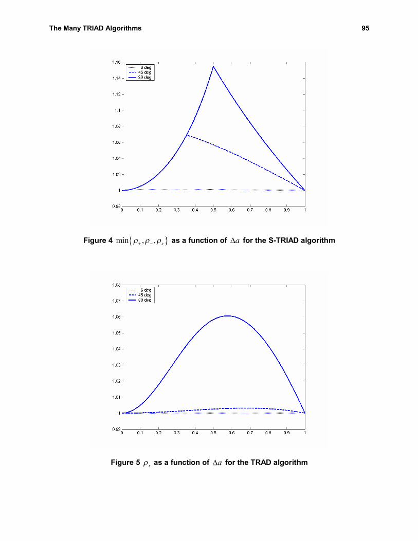
Unlike ρ± , the third figure of merit sρ depends on the type of TRIAD algorithm. For the S-

TRIAD, sρ exhibits two special traits: (1) it is independent of the angle between observed vectors (Fig. 3), and (2) at some threshold value, a a∆ = ∆ , it becomes equal to ρ− . In other words, for sufficiently dissimilar measurements, i.e. a a∆ > ∆ , the lower bound of the S-TRIAD errors becomes limited by ρ− instead of sρ . The threshold value a∆ grows from 0 to 1/ 2 as the two observed vectors vary from collinear to perpendicular (Fig. 4). The TRAD algorithm yields sρ that remains very close (within

6%≈ ) to the lowest possible value (Fig. 5).

The Many TRIAD Algorithms 93

The next figure of merit RSSρ characterizes the average error level of each algorithm. With the

exception of TRIAD-II, the rest of the TRIAD estimators yield RSSρ close to that of the Wahba estimator

(Figs. 6, 7). TRIAD-II yields a progressively worse performance as the disparity between the accuracies

of the observed vectors widens (Fig. 7). This is expected as the TRIAD-II algorithm favors the lower

accuracy vector. An alternate figure of merit

22

22 2

( ) 1 2 2

cos 21

2 1

VRSS

RSS Wahba

a n

a a

ϕρδρ

ρ

∆ −= − =

+

s

s (70)

can be used to highlight the relative increase in the error level of the TRIAD estimators compared to the

Wahba estimator (Fig. 8).

Figure 1 ρ+ as a function of a∆ for all TRIAD algorithms

94 Tanygin and Shuster

Figure 2 ρ− as a function of a∆ for all TRIAD algorithms

Figure 3 sρ as a function of a∆ for the S-TRIAD algorithm for any angle between the two vectors

The Many TRIAD Algorithms 95

Figure 4 { }min , , sρ ρ ρ+ − as a function of a∆ for the S-TRIAD algorithm

Figure 5 sρ as a function of a∆ for the TRAD algorithm

96 Tanygin and Shuster

Figure 6 RSSρ as a function of a∆ for a 45-deg angle between the two vectors

Figure 7 RSSρ as a function of a∆ for a 45-deg angle between the two vectors

The Many TRIAD Algorithms 97

Figure 8 δρ in % as a function of a∆ for a 45-deg angle between the two vectors

CONCLUSIONS

We have developed a general formulation of the TRIAD algorithm which encompasses all variations of the TRIAD algorithm and which permits a unified treatment of the covariance analysis of these algorithms. These different TRIAD algorithms differ only in the value of a single parameter, the mixing angle. By finding the optimal value of this angle which minimizes the Wahba cost function over the continuum of TRIAD algorithms we have obtained the optimal TRIAD algorithm, which differs from the optimal Wahba estimate only by terms of higher order in the measurement noise.

Had this estimator been discovered in 1970, it would have been an important practical result. Today, given the exponentially increasing computational power and the availability of fast optimal algorithms that can accommodate any number of measurements, its importance is largely of theoretical interest only, but certainly of great theoretical interest. No doubt, the TRIAD algorithm has still more secrets to reveal.

REFERENCES

1. H. D. Black, “A Passive System for Determining the Attitude of a Satellite,” AIAA Journal, Vol. 2, July 1964, pp. 1350–1351.

2. M. D. Shuster, and S. D. Oh, “Three-Axis Attitude Determination from Vector Observations,” Journal of Guidance and Control, Vol. 4, No. 1, January–February 1981, pp. 70–77.

98 Tanygin and Shuster

3. G. Wahba, “Problem 65-1: A Least Squares Estimate of Spacecraft Attitude,” Siam Review, Vol. 7, No. 3, July 1965, pp. 409.

4. M. D. Shuster, “Attitude Determination in Higher Dimensions,” Journal of Guidance, Control and Dynamics, Vol. 16, No. 2, March–April 1993, pp. 393–395.

5. F. L. Markley, “Attitude Determination using Vector Observations: a Fast Optimal Matrix Algorithm,” The Journal of the Astronautical Sciences, Vol. 41, No. 2, April-June 1993, pp. 261–280.

6. D. Mortari, “EULER-2 and EULER-n Algorithms for Attitude Determination from Vector Observations,” Space Technology, Vol. 16, Nos. 5-6, 1996, pp. 317-321.

7. F. L. Markley, “Attitude Determination using Two Vector Measurements,” Proceedings, Flight Mechanics Symposium, NASA Goddard Space Flight Center, Greenbelt, MD, May 1999, NASA Conference Publication NASA/CP-19989-209235, pp. 39–52.

8. M. D. Shuster, “Attitude Analysis in Flatland: the Plane Truth,” The Journal of the Astronautical Sciences, Vol. 52, Nos. 1-2, January–June 2004, pp. 195–209.

9. Y. Cheng, and M. D. Shuster, “QUEST and the Anti-QUEST: Good and Evil Attitude Estimation,” The Journal of the Astronautical Sciences, Vol. 53, No. 3, July–September 2005, pp. 337–351.

10. M. D. Shuster, “The TRIAD Algorithm as Maximum Likelihood Estimation,” The Journal of the Astronautical Sciences, Vol. 54, No. 1, January–March 2006, pp. 113–123.

11. G. M. Lerner, “Three-Axis Attitude Determination,” in J.R. Wertz, (ed.), Spacecraft Attitude Determination and Control, Springer Scientific + Business Media, 1978, pp.420–428.

12. F. L. Markley, and D. Mortari, “Quaternion Attitude Estimation using Vector Measurements,” The Journal of the Astronautical Sciences, Vol. 48, Nos. 2 and 3, April–September 2000, pp. 359–380.

13. M. D. Shuster, “SCAD – A Fast Algorithm for Star-Camera Attitude Determination,” The Journal of the Astronautical Sciences, Vol. 52, No. 3, July–September 2004, pp. 391–404.

14. M. D. Shuster, “The Equivalent-Vector Method,” The Journal of the Astronautical Sciences, Vol. 55, No. 1, January–March 2007 (to appear).

15. M. D. Shuster, “The Optimization of TRIAD,” The Journal of the Astronautical Sciences, Vol. 55, No. 2, April–June 2007 (to appear).

16. M. D. Shuster, “A Survey of Attitude Representations,” The Journal of the Astronautical Sciences, Vol. 41, No. 4, October–December 1993, pp. 439–517.

17. M. D. Shuster, “Maximum Likelihood Estimation of Spacecraft Attitude,” The Journal of the Astronautical Sciences, Vol. 37, No. 1, January–March 1989, pp. 79–88.

18. H. W. Sorensen, Parameter Estimation, New York, Marcel Dekker, 1980.

The Many TRIAD Algorithms 99

APPENDIX: SPECTRAL DECOMPOSITION OF THE G-TRIAD COVARIANCE MATRIX

We can take advantage of the structure of the G-TRIAD covariance matrix (Eq.(43)) to partition space into two subspaces: one that lies along the vector 2s , and the other that is perpendicular to it. The

characteristic vector 2ˆ ˆ

s =e s has the associated characteristic value given by

( )( )2T G-TRIAD 2 G-TRIAD2 2

ˆ ˆ 1s totPλ σ δ= = +ξξs s (A.1)

The remaining two characteristic vectors, that must be perpendicular to 2s , can be parameterized using

the mutually orthogonal vectors 1W and 3s , and the rotational angle ψ , i.e.

( )( )1 3 1 21ˆ ˆ ˆˆ ˆ

V VV

c s s c sψ ψ ψ ψ ψα ββ

≡ + = + −e W s W W (A.2)

with coscψ ψ≡ and sinsψ ψ≡ . Then,

2

G-TRIAD1 22

2 1

ˆ ˆˆ V Vtot

V

c c sP

a aψ ψ ψα βσ

β−

= +

ξξ e W W (A.3)

Using the condition that direction of the characteristic vector remains unchanged by the matrix product, we obtain from equations (A.2) and (A.3)

( )( )1 2 0V V V Va c s a s c c sψ ψ ψ ψ ψ ψα β α β+ + − = (A.3)

which leads to two possible solutions for the characteristic vectors

* *1 3

ˆˆ ˆc sψ ψ+ = +e W s and * *1 3

ˆˆ ˆs cψ ψ− = −e W s (A.4ab)

with

( )( )

*22 2

1tan 2 V V

V V

aaα β

ψα β

− ∆= −

+ ∆ (A.5)

Once the characteristic vectors are found, the associated characteristic values follow directly from

( )22T G-TRIAD

1 2 2 21 2 2

1ˆ ˆ 1 1 42

totP a aa aσ

λ+ + += = + −ξξe e ss

(A.6a)

( )22T G-TRIAD

1 2 2 21 2 2

1ˆ ˆ 1 1 42

totP a aa aσ

λ− − −= = − −ξξe e ss

(A.6b)