A visual analytics framework for cluster analysis of DNA microarray data

Expert Systems with Applications xxx (2012) xxx–xxx

Contents lists available at SciVerse ScienceDirect

Expert Systems with Applications

journal homepage: www.elsevier .com/locate /eswa

A visual analytics framework for cluster analysis of DNA microarray data

José A. Castellanos-Garzón a,⇑, Carlos Armando García b, Paulo Novais c, Fernando Díaz a

a Department of Computer Science, University of Valladolid, University School of Computer Science, Plaza Santa Eulalia 9-11, 40005 Segovia, Spainb Department of Computer Science and Automatics, University of Salamanca, Faculty of Sciences, Plaza de los Caídos s/n, 37008 Salamanca, Spainc Department of Informatics, Universidade do Minho, Campus of Gualtar, 4710-057 Braga, Portugal

a r t i c l e i n f o a b s t r a c t

Keywords:Data miningDNA-microarraysCluster analysisVisual analyticsMetric spacesBoundary pointsSurface reconstruction

0957-4174/$ - see front matter � 2012 Elsevier Ltd. Ahttp://dx.doi.org/10.1016/j.eswa.2012.08.038

⇑ Corresponding author.E-mail addresses: [email protected] (J.A. Caste

@usal.es (C.A. García), [email protected] (P. Novais),

Please cite this article in press as: Castellanos-Gwith Applications (2012), http://dx.doi.org/10.10

Cluster analysis of DNA microarray data is an important but difficult task in knowledge discovery pro-cesses. Many clustering methods are applied to analysis of data for gene expression, but none of themis able to deal with an absolute way with the challenges that this technology raises. Due to this, manyapplications have been developed for visually representing clustering algorithm results on DNA micro-array data, usually providing dendrogram and heat map visualizations. Most of these applications focusonly on the above visualizations, and do not offer further visualization components to the validate theclustering methods or to validate one another. This paper proposes using a visual analytics frameworkin cluster analysis of gene expression data. Additionally, it presents a new method for finding clusterboundaries based on properties of metric spaces. Our approach presents a set of visualization compo-nents able to interact with each other; namely, parallel coordinates, cluster boundary genes, 3D clustersurfaces and DNA microarray visualizations as heat maps. Experimental results have shown that ourframework can be very useful in the process of more fully understanding DNA microarray data. Thesoftware has been implemented in Java, and the framework is publicly available at http://www.analiticavisual.com/jcastellanos/3DVisualCluster/3D-VisualCluster.

� 2012 Elsevier Ltd. All rights reserved.

1. Introduction

Advances in bioinformatics have resulted in large quantities ofbiological data, which have been made available in various publicdatabases. Biologists often wish to analyse these databases tounderstand the relationships within them. Traditional approachesare oriented towards discovering evolutionary relationships be-tween genes or proteins by analysing their sequence and structuralsimilarities (Schroeder, Gilbert, Helden, & Noy, 2001).

Visual data exploration provides a means of verifying criteria orhypotheses formulated on evolutionary processes. However, thismay also be accomplished using automatic techniques from statis-tics or machine learning. Visual data exploration usually allowsfaster data exploration and often provides better results, especiallyin cases where automatic algorithms fail (Keim, 2002). Usually, thiskind of data exploration involves a three-step process: overview,zooming and filtering, and then accessing details on demand(Maletic, Marcus, & Collard, 2002; Shneiderman, 1996).

A single DNA microarray experiment typically evaluates a largenumber of DNA sequences (genes, cDNA clones, or expressedsequence tags) under several conditions. These conditions may

ll rights reserved.

llanos-Garzón), [email protected] (F. Díaz).

arzón, J. A., et al. A visual analy16/j.eswa.2012.08.038

sometimes be a series from throughout a biological process (e.g.,the yeast-cellcycle) or a collection of different tissue samples(e.g., normal versus cancerous tissues). In this research, we focuson cluster analysis (Jain & Dubes, 1998, Jain, Murty, & Flynn,1999; Kaufman & Rousseeuw, 2005; Pedrycz, 2005) done withoutconsidering distinctions between different types of DNA se-quences, which are generically called genes. Similarly, the condi-tions refer uniformly to all kinds of experimental conditions,called samples or simply conditions. On the other hand, our DNAmicroarray analysis focuses on gene-based clustering analysis,but it is also possible to perform sample-based clustering analysisby computing the transpose matrix of the gene expression matrix(Belacel, Wang, & Cuperlovic-Culf, 2006; Jiang, Tang, & Zhang,2004).

Because visual data exploration is proving to be very useful in thefield of bioinformatics (Baldin & Brunak, 1998; Pal, Bandyopadhyay,& Murthy, 2006), then combining it with data mining techniquesfor gene expression data can provide knowledge of processesthat take place at the cellular level (Berrar, Dubitzky, & Granzow,2003; Chan & Kasabov, 2004; Geoffrey, Do, & Ambroise, 2004; Han& Kamber, 2006; Jiang et al., 2004; Olson & Delen, 2008; Speed,2003). Genes with similar expression levels can be groupedaccording to cellular functions. This approach may disclose informa-tion about the functions of many genes for which no previousinformation is available (Eisen, Spellman, Brown, & Botstein,

tics framework for cluster analysis of DNA microarray data. Expert Systems

http://www.analiticavisual.com/jcastellanos/3DVisualCluster/3D-VisualCluster


http://dx.doi.org/10.1016/j.eswa.2012.08.038

mailto:[email protected]

mailto:CarlosGarcia @usal.es

mailto:CarlosGarcia @usal.es




http://www.sciencedirect.com/science/journal/09574174

http://www.elsevier.com/locate/eswa


2 J.A. Castellanos-Garzón et al. / Expert Systems with Applications xxx (2012) xxx–xxx

1998; Tavazoie, Hughes, Campbell, Cho, & Church, 1999). Moreover,visual analytics can be used to discover information about thevariety of available clustering algorithms. Biologists often haveproblems selecting the most appropriate algorithm from a givengene expression data set, since no single algorithm is best in everyaspect (Jiang et al., 2004).

This paper introduces visual data exploration for aggregating,summarizing and visualizing information generated during inter-active cluster analysis on DNA microarray data (Jain & Dubes,1998, 1999; Kaufman & Rousseeuw, 2005; Pedrycz, 2005). As a re-sult of our framework, we have developed a prototype tool (called3D-VisualCluster or 3D-VC for short), which is able to exploredendrograms, clusterings and clusters interactively with differentviews (Schroeder et al., 2001; Keim, 2002). This prototype usesprincipal component analysis (PCA, Jolliffe, 2002) to reduce datadimensionality to R3, so that a first approximation of the data dis-tribution can be analysed on a 3D scatter plot. Furthermore, paral-lel coordinate visualization (Inselberg & Dimsdale, 1990) and DNAmicroarray data views are presented using a colour scale corre-sponding to gene expression levels (heat map). Note that connect-ing multiple visualizations through interactive linking providesmore information than considering the visualization componentsindependently.

Additionally, a new method of computing cluster boundarypoints is defined using the boundary definition of metric spaces.With this method, we can display and analyse the boundary genesof a cluster, 3D cluster surfaces, and 3D representations of refer-ence partitions. Together, these can be seen as a new approachfor visually comparing clusterings and reference partitions. Finally,the usefulness of our approach to gene expression research isshown by applying several clustering methods to real data.

To conclude, we explain the structure followed by this paper.Section 2 describes the related work, which deals with the existingtools and components of visualization from DNA microarray data,providing a comparative table of visual components that includesour tool. Furthermore, a background on boundary points has alsobeen given. Section 3 introduces the framework for cluster analy-sis, which provides two algorithms (boundary point and surfacereconstruction algorithm) based on the theory of metric spaces.Section 4 explains the 3D-VC tool as a result of our frameworkand gives a methodology to follow (by a set of tasks) to visuallyanalyse the results of the clustering methods. Section 5 outlinesthe results and discussion of our framework (by the 3D-VC tool)applied to a case study on a public data set of DNA microarray. Sec-tion 6 describes the conclusions of our proposal. Appendices A andB respectively give concepts on metric spaces and the theoreticalresults of Section 3 on which the framework is based.

2. Related work

Cluster analysis is the technique of finding groupings withindata in such a way that these groupings make sense in the contextof a particular problem. Issues such as feature selection, missingdata imputation, outliers and noise treatment, choosing a suitablemetrics and the optimal cluster number are still open challenges.Cluster analysis involves three main stages: pre-processing, clusteranalysis and cluster validation. The last stage includes the selectionand application of cluster validity techniques, generally divided ininternal and external measures (Datta & Datta, 2003; Handl,Knowles, & Kell, 2005; Jiang et al., 2004; Yeung, Haynor, & Ruzzo,2001). Visual validity can be added as a subsequent step afterapplying the cluster validity measures, and the use of new anddifferent visualization components may help resolve the abovementioned problems while also validating the statistical measures.

Please cite this article in press as: Castellanos-Garzón, J. A., et al. A visual analywith Applications (2012), http://dx.doi.org/10.1016/j.eswa.2012.08.038

Visual validation approaches applied to DNA microarray datahave generated several commercially and publicly available toolsfor data visualization (Eisen, xxxx; Reich, Ohm, Tamayo, Angelo,& Mesirov, 2004; Saeed et al., 2003; Seo & Shneiderman, 2002;Seo & Shneiderman, 2005; Weber et al., 2009). These tools havethe following drawbacks. Most of them do not implement dimen-sionality reduction to represent data on a 3D scatter plot, and thetools that do have this functionality go no further than showingdata-points. On the other hand, these tools implement a smallnumber of pre-fitted clustering methods, which raises problemswhen validating new methods. Moreover, they do not offer a visualinteraction framework that is able to validate clustering resultsaccording to a reference partition.

Based on the above discussion, we have designed the main fea-tures of our prototype so as to compare it with five of the previ-ously mentioned tools. These visualization components (orfeatures) are listed below with comments about their expected im-pact on the above mentioned problems in cluster analysis.

1. DNA microarray data dendrogram analysis (MDA). This refers tothe ability of the tested tools to incorporate dendrogram analy-sis, in the sense that the user can select and evaluate differentcut-off levels in the dendrogram. This can help the users findthe most suitable number of clusters, and offers a global viewof the constructed cluster hierarchy and the associated heatmap for the available data.

2. Scatter plot analysis (SPA). This is the ability of the tool toimplement some type of scatter plot analysis on microarraydata. This kind of graph depends on the level chosen in dendro-gram analysis and can also be useful for validating the clusternumber. Moreover, a scatter plot allows us to detect outliersor noise in the data, as well as to validate the inter-cluster dis-tance used by the clustering methods.

3. Microarray parallel coordinates (MPC). Implementation of par-allel coordinate analyses on the clusters represented as pointsand heat maps. With this kind of representation, a user can val-idate cluster homogeneity (cluster internal quality) by comple-menting the dendrogram and scatter plot analysis.

4. Microarray statistical analysis (MSA). Whether the tool inte-grates other statistical data analyses. This component can pro-vide preparatory data analysis, such as feature, metric andclustering method selection.

5. Microarray data clustering methods (MCM). Whether the toolcouples clustering methods. This component allows selectionof a clustering method and compares the results with othermethods. In this way, the method that best fits the data canbe chosen, and thus implicitly includes the selection of dataand inter-cluster distance.

Based on these points, Table 1 compares our prototype (3D-VC)with tools from Eisen (xxxx), Saeed et al. (2003), Reich et al. (2004),Seo and Shneiderman (2002), Weber et al. (2009), with visualiza-tion items as the rows and tool references as the columns. A checkmark (U) is used to indicate that a tool provides the specifiedproperty for that row, and ‘‘�’’ indicates that it does not providethis property. Additionally, the value ‘‘b-in’’ means that the toolimplements the corresponding features (clustering methods or sta-tistical measures) as built-in functionalities, and hence cannot beextended without a considerable modification of the software.The value ‘‘ext’’ means the opposite of ‘‘b-in’’, since the tool hasthe ability of extending its functionality by linking with externalsoftware components (for example, through an R language API).

Some of these visual components can be improved by extendingtheir functionality, as in the case of Visual Exploration 3D (Weberet al., 2009) and the proposed 3D-VC, which both implement a 3D



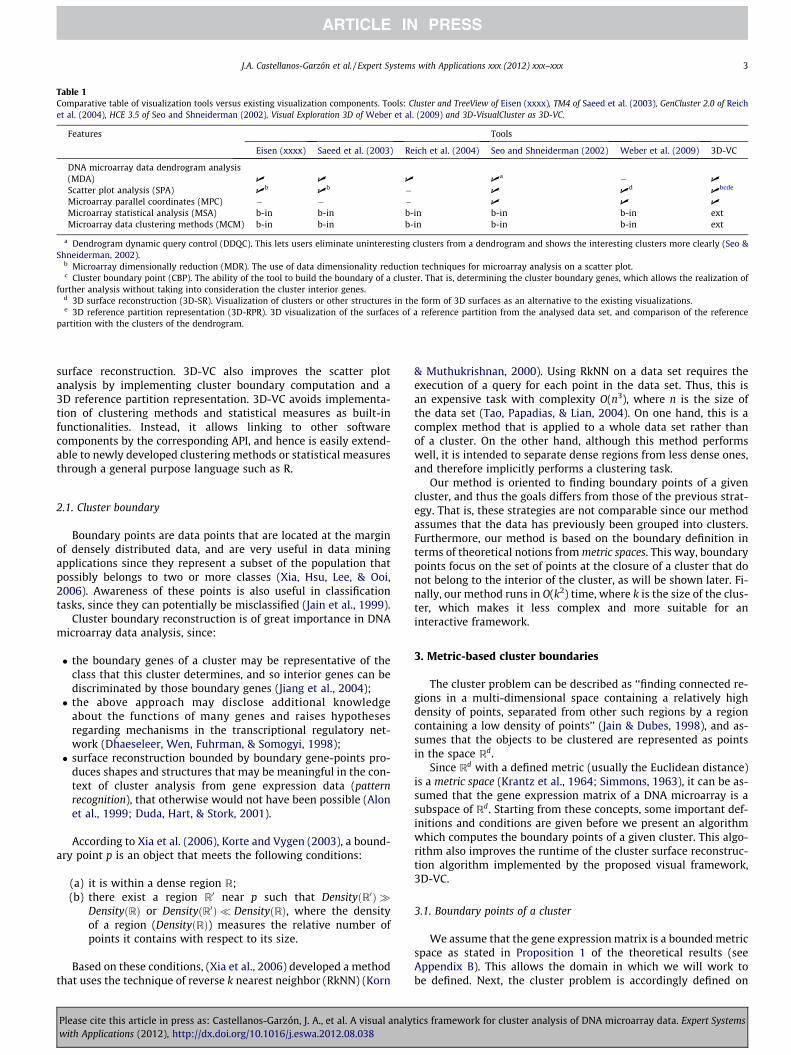
Table 1Comparative table of visualization tools versus existing visualization components. Tools: Cluster and TreeView of Eisen (xxxx), TM4 of Saeed et al. (2003), GenCluster 2.0 of Reichet al. (2004), HCE 3.5 of Seo and Shneiderman (2002), Visual Exploration 3D of Weber et al. (2009) and 3D-VisualCluster as 3D-VC.

Features Tools

Eisen (xxxx) Saeed et al. (2003) Reich et al. (2004) Seo and Shneiderman (2002) Weber et al. (2009) 3D-VC

DNA microarray data dendrogram analysis(MDA) U U U U

a � U

Scatter plot analysis (SPA) Ub

Ub � U U

dU

bcde

Microarray parallel coordinates (MPC) � � � U U U

Microarray statistical analysis (MSA) b-in b-in b-in b-in b-in extMicroarray data clustering methods (MCM) b-in b-in b-in b-in b-in ext

a Dendrogram dynamic query control (DDQC). This lets users eliminate uninteresting clusters from a dendrogram and shows the interesting clusters more clearly (Seo &Shneiderman, 2002).

b Microarray dimensionally reduction (MDR). The use of data dimensionality reduction techniques for microarray analysis on a scatter plot.c Cluster boundary point (CBP). The ability of the tool to build the boundary of a cluster. That is, determining the cluster boundary genes, which allows the realization of

further analysis without taking into consideration the cluster interior genes.d 3D surface reconstruction (3D-SR). Visualization of clusters or other structures in the form of 3D surfaces as an alternative to the existing visualizations.e 3D reference partition representation (3D-RPR). 3D visualization of the surfaces of a reference partition from the analysed data set, and comparison of the reference

partition with the clusters of the dendrogram.

J.A. Castellanos-Garzón et al. / Expert Systems with Applications xxx (2012) xxx–xxx 3

surface reconstruction. 3D-VC also improves the scatter plotanalysis by implementing cluster boundary computation and a3D reference partition representation. 3D-VC avoids implementa-tion of clustering methods and statistical measures as built-infunctionalities. Instead, it allows linking to other softwarecomponents by the corresponding API, and hence is easily extend-able to newly developed clustering methods or statistical measuresthrough a general purpose language such as R.

2.1. Cluster boundary

Boundary points are data points that are located at the marginof densely distributed data, and are very useful in data miningapplications since they represent a subset of the population thatpossibly belongs to two or more classes (Xia, Hsu, Lee, & Ooi,2006). Awareness of these points is also useful in classificationtasks, since they can potentially be misclassified (Jain et al., 1999).

Cluster boundary reconstruction is of great importance in DNAmicroarray data analysis, since:

� the boundary genes of a cluster may be representative of theclass that this cluster determines, and so interior genes can bediscriminated by those boundary genes (Jiang et al., 2004);� the above approach may disclose additional knowledge

about the functions of many genes and raises hypothesesregarding mechanisms in the transcriptional regulatory net-work (Dhaeseleer, Wen, Fuhrman, & Somogyi, 1998);� surface reconstruction bounded by boundary gene-points pro-

duces shapes and structures that may be meaningful in the con-text of cluster analysis from gene expression data (patternrecognition), that otherwise would not have been possible (Alonet al., 1999; Duda, Hart, & Stork, 2001).

According to Xia et al. (2006), Korte and Vygen (2003), a bound-ary point p is an object that meets the following conditions:

(a) it is within a dense region R;(b) there exist a region R0 near p such that DensityðR0Þ �

DensityðRÞ or DensityðR0Þ � DensityðRÞ, where the densityof a region (DensityðRÞ) measures the relative number ofpoints it contains with respect to its size.

Based on these conditions, (Xia et al., 2006) developed a methodthat uses the technique of reverse k nearest neighbor (RkNN) (Korn


& Muthukrishnan, 2000). Using RkNN on a data set requires theexecution of a query for each point in the data set. Thus, this isan expensive task with complexity O(n3), where n is the size ofthe data set (Tao, Papadias, & Lian, 2004). On one hand, this is acomplex method that is applied to a whole data set rather thanof a cluster. On the other hand, although this method performswell, it is intended to separate dense regions from less dense ones,and therefore implicitly performs a clustering task.

Our method is oriented to finding boundary points of a givencluster, and thus the goals differs from those of the previous strat-egy. That is, these strategies are not comparable since our methodassumes that the data has previously been grouped into clusters.Furthermore, our method is based on the boundary definition interms of theoretical notions from metric spaces. This way, boundarypoints focus on the set of points at the closure of a cluster that donot belong to the interior of the cluster, as will be shown later. Fi-nally, our method runs in O(k2) time, where k is the size of the clus-ter, which makes it less complex and more suitable for aninteractive framework.

3. Metric-based cluster boundaries

The cluster problem can be described as ‘‘finding connected re-gions in a multi-dimensional space containing a relatively highdensity of points, separated from other such regions by a regioncontaining a low density of points’’ (Jain & Dubes, 1998), and as-sumes that the objects to be clustered are represented as pointsin the space Rd.

Since Rd with a defined metric (usually the Euclidean distance)is a metric space (Krantz et al., 1964; Simmons, 1963), it can be as-sumed that the gene expression matrix of a DNA microarray is asubspace of Rd. Starting from these concepts, some important def-initions and conditions are given before we present an algorithmwhich computes the boundary points of a given cluster. This algo-rithm also improves the runtime of the cluster surface reconstruc-tion algorithm implemented by the proposed visual framework,3D-VC.

3.1. Boundary points of a cluster

We assume that the gene expression matrix is a bounded metricspace as stated in Proposition 1 of the theoretical results (seeAppendix B). This allows the domain in which we will work tobe defined. Next, the cluster problem is accordingly defined on




the bounded metric space. Finally, a proposition about whether acluster is opened or closed is presented. This proposition is usefulfor defining the problem of cluster boundary points.

In what follows, the set Gdn denotes a bounded subspace of

Rd with an induced metric q, where d is the dimension and nis the number of genes. That is, G

dn with the metric q is a

bounded discrete metric space, called the gene metric space.The methods introduced in this section are based on the defini-tions and proofs given in the section entitled metric spaces (seeAppendix A).

We can now state the cluster problem on Gdn, which is defined

according to Jain and Dubes (1998) as follows.

Definition 1. Cluster problem on Gdn.

Let Gdn be a metric space. Then a partition C of G

dn is a collection

of subsets {C1,C2, . . . ,Cm} of Gdn satisfying:

Ci \ Cj ¼ ;; 8i; j 2 ½1;m�; i – j; and

Gdn ¼

[m

i¼1

Ci; i 2 ½1;m�:

A partition C of Gdn for which the above definition holds is called a

clustering, and the subsets Ci are called clusters. The cluster problemconsists of finding a suitable clustering of G

dn satisfying a similarity

criteria between genes in Gdn, which is represented in most cases as

a distance function q.This clustering definition is very important since different

clustering definitions could yield distinct results for the clusterproperties in G

dn. Note that in our case, a cluster C of a clustering

in a metric space Gdn is a special type of subset in G

dn where no

gene of C belongs to a different cluster of C in the sameclustering.

From Definitions 9 and 10 in Appendix A, we can prove that acluster C of G

dn is a closed set (see Proposition 2 in Appendix B).

As a consequence of this result, C is not an open set in Gdn and

the frontier of C coincides with its boundary (Definitions 8 and12). This proposition is very important since if C was an opencluster, then it makes no sense to think about its boundarypoints.

3.2. Multidimensional algorithm to obtain cluster boundaries

The boundary points of a subset in a d-dimensional space arevery important in data mining, since analysing these points canreveal information about the problem being addressed (Jianget al., 2004; Xia et al., 2006). To compute the boundary of a clus-ter it is necessary to introduce the concept of an extreme gene,which is fundamental in searching for cluster boundary points.An ith extreme gene (or extreme gene) of a cluster is a gene (re-garded as a vector in G

dn) whose ith component is either greater

or less than that for the remaining genes in the cluster. The setof all extreme genes of a cluster C is denoted by ExmC (see Def-inition 13 in Appendix B). An important result from the abovestatement is that an extreme gene of a cluster belongs to theboundary of such a cluster (as stated in Proposition 3 in Appen-dix B). Note that if C is a cluster of G

dn then Exm C # BdC and

Card(ExmC) 6 2d (Card is the cardinality of ExmC), where BdCis the boundary of C.

We now introduce an algorithm called ClusterBoundary to findthe boundary points of a cluster (note that character % in the algo-rithm indicates a comment). In contrast with other approaches, ourboundary definition focuses on the concept of a boundary in a met-ric space, namely the set of points in the closure of a cluster that donot belong to the interior of the cluster.


3.2.1. ClusterBoundary algorithm

Input: C a cluster in Gdn and q the metric defined on G

dn.

Output: BdC, the boundary of the cluster C1. BdC = ;;2. while C – ; do3. % Module (I)- Find all ith extreme genes in C.4. % max.exm, min.exm search for the maximal and minimal

ith extreme genes5. % respectively.6. ExmC = ;;7. for all i 2 [1,d] and C – ; do8. ExmC :¼ ExmC

Sfgi� :¼ max :exmðC; iÞ; gi

� :¼min :exmðC n fgi

�g; iÞg;9. C :¼ C n fgi

�; gi�g;

10. endfor11. BdC:¼BdC

SExmC;

12. % Module (II)-Compute the centroid (middle point) ofExmC.

13. a:¼ centroid (ExmC);14. % Module (III)-Compute the mid-points between

extreme point pairs except

15. % for gi� and gj

� where i = j.16. Pm :¼ ;;18. for all i 2 [1,d] do19. Pm :¼ Pm

Sfmiddle:pointðgi

�; gÞjg 2 ExmC n fgi�; g

i�gg;

20. Pm :¼ PmSfmiddle:pointðgi

�; gÞjg 2 ExmC n fgi�; g

i�gg;

21. endfor22. % Module (IV)-Compute the radius of a ball with interior

points in C as follows:23. choose either r:¼min{q(a,p)jp 2 Pm} or

r :¼mean{q(a,p)jp 2 Pm}or24. r :¼max{q(a,p)jp 2 Pm};25. % choosing one of the above radiuses determines the

type of approximation26. % to the boundary of the cluster27. % Remove interior points of the ball with center a and

radius r28. C :¼ CnN(a,r);29. endwhile30. end

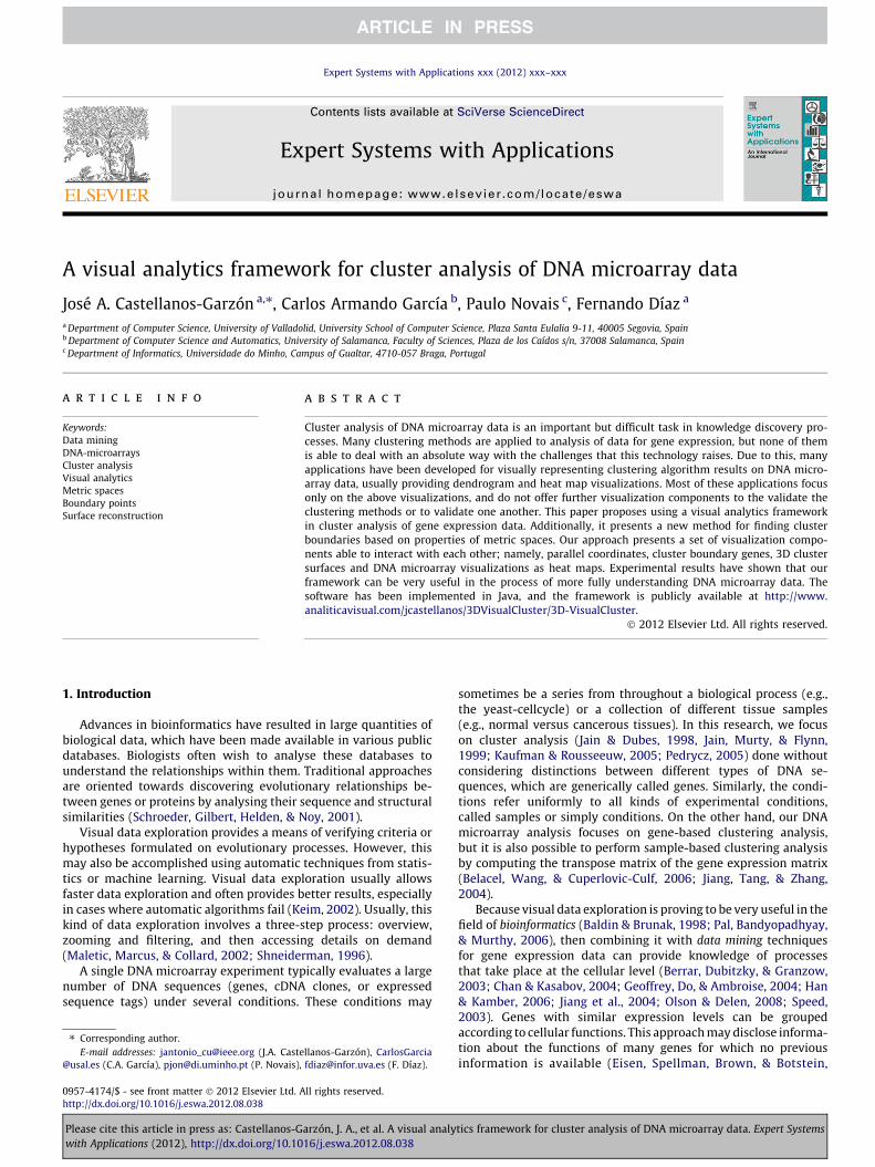
The ClusterBoundary algorithm is divided in four fundamentalmodules, which are explained using an example of a cluster in R3.Module (I) (lines 3–11) carries out a search for extreme points asshown in Fig. 1a. In this figure, the extreme points of a hypotheticalcluster are highlighted in red. At each iteration of the algorithm, thecluster boundary is incrementally built from the extreme points(based on Proposition 3 in Appendix B). Module (II) (lines 12–13)computes the centroid of the extreme points, which will be the cen-tre of the interior point ball as shown in Fig. 1b. Note that the linesdrawn between the extreme points form an eighth-sided polygonencloses most of the points. Module (III) (lines 14–21) computesthe mid-points between each extreme point-pair, except for thepairs ðgi

�; gj�Þ where i = j. Fig. 1c shows this, as well as the possible

radiuses computed from the centroid to the mid-points. Module(IV) (lines 22–28) determines the radius of the ball with the centrealready computed in module (II). The radius can be chosen as eitherthe minimal, the mean or the maximal distance between the cen-troid and the points in the set of mid-points Pm. The option of choos-ing different radiuses is related to the strategy for constructing the



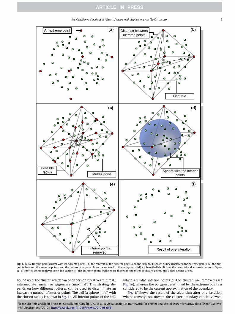
Fig. 1. (a) A 3D gene-point cluster with its extreme points; (b) the centroid of the extreme points and the distances (shown as lines) between the extreme points; (c) the mid-points between the extreme points, and the radiuses computed from the centroid to the mid-points; (d) a sphere (ball) built from the centroid and a chosen radius in Figurec; (e) interior points removed from the sphere; (f) the extreme points from (e) are moved to the set of boundary points, and a new cluster arises.


boundary of the cluster, which can be either conservative (minimal),intermediate (mean) or aggressive (maximal). This strategy de-pends on how different radiuses can be used to discriminate anincreasing number of interior points. The ball (a sphere in R3) withthe chosen radius is shown in Fig. 1d. All interior points of the ball,


which are also interior points of the cluster, are removed (seeFig. 1e), whereas the polygon determined by the extreme points isconsidered to be the current approximation of the boundary.

Fig. 1f shows the result of the algorithm after one iteration,where convergence toward the cluster boundary can be viewed.



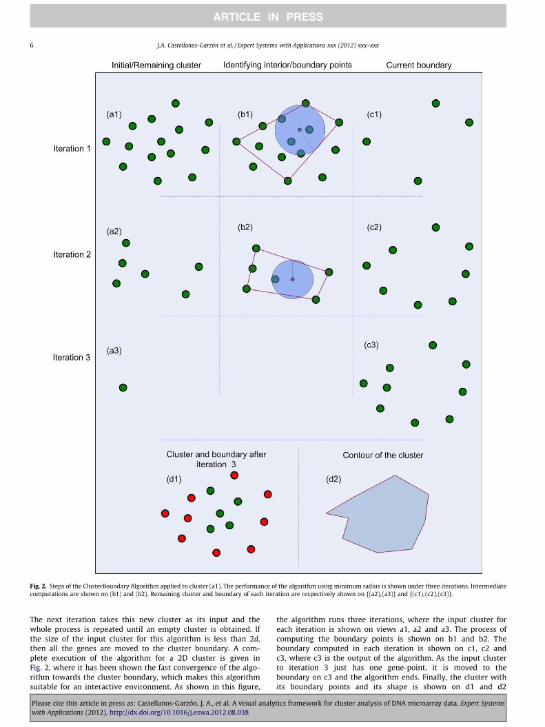
Fig. 2. Steps of the ClusterBoundary Algorithm applied to cluster (a1). The performance of the algorithm using minimum radius is shown under three iterations. Intermediatecomputations are shown on (b1) and (b2). Remaining cluster and boundary of each iteration are respectively shown on {(a2), (a3)} and {(c1), (c2), (c3)}.


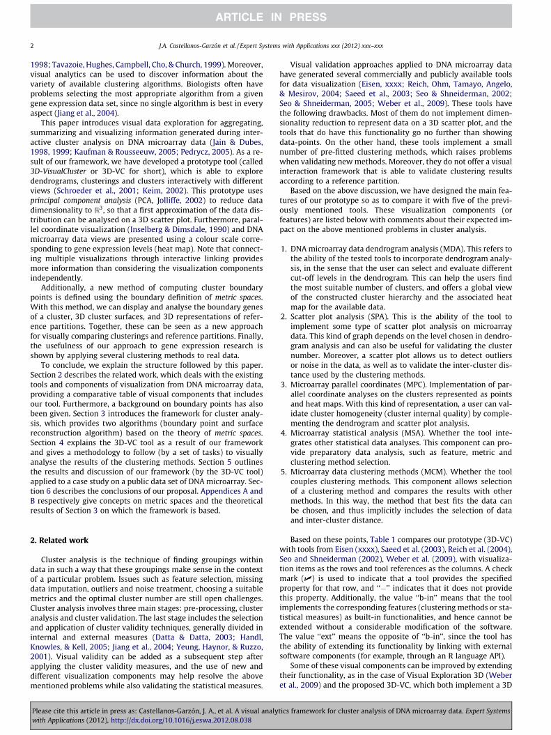
The next iteration takes this new cluster as its input and thewhole process is repeated until an empty cluster is obtained. Ifthe size of the input cluster for this algorithm is less than 2d,then all the genes are moved to the cluster boundary. A com-plete execution of the algorithm for a 2D cluster is given inFig. 2, where it has been shown the fast convergence of the algo-rithm towards the cluster boundary, which makes this algorithmsuitable for an interactive environment. As shown in this figure,


the algorithm runs three iterations, where the input cluster foreach iteration is shown on views a1, a2 and a3. The process ofcomputing the boundary points is shown on b1 and b2. Theboundary computed in each iteration is shown on c1, c2 andc3, where c3 is the output of the algorithm. As the input clusterto iteration 3 just has one gene-point, it is moved to theboundary on c3 and the algorithm ends. Finally, the cluster withits boundary points and its shape is shown on d1 and d2




respectively. Note that the algorithm converges towards theboundary of the cluster in a few iterations.

From the performance and the runtime complexity (Aho,Hopcroft, & Ullman, 1983; Gács & Lovász, 1999; Wilf, 1994) ofClusterBoundary, we have that the number of mid-points in Pm isbounded by 2d(d � 1) (see Proposition 4 in Appendix B). Hence,the runtime of this algorithm in the worst case scenario is O(k2),where k is the size of the input cluster (for a formal proof seeProposition 5 in Appendix B).

3.3. Surface reconstruction based on boundary points

Surface reconstruction considers the extraction of shape infor-mation from a point set. These point sets often contain noise,redundancy and systematic variation arising from the experimen-tal procedure. Therefore, a general approach to reconstructingsurfaces is a challenging problem (Hoppe et al., 1994; Heckel,Hamann, & Uva, 1997).

The goal of surface reconstruction methods can be described asfollows: given a set of sample points X assumed to lie on or near anunknown surface U, construct a surface model S approximating U(Hoppe, DeRose, Duchamp, McDonald, & Stuetzle, 1992, 1994;Maric, Maric, Mijajlovic, & Jovanovic, 2005).

The proposed algorithm is a modification of the one presentedin Berg, Cheong, Kreveld, and Overmars (2008), Boissonnat andTeillaud (2006), which reconstructs convex hulls. In general, sincemany surfaces are not convex hulls, we provide a version thattransforms the basis algorithm to obtain non-convex hulls. As ageneral schema, the algorithm projects boundary points of a clus-ter onto the plane, and determines the convex boundary points.Second, the algorithm inserts the remaining non-convex bound-ary points into the list of convex boundary points. Finally, thealgorithm returns an ordered list of boundary points which isused to establish the connectivity of points in a 3D dimensionalspace.

The first aim of this algorithm is to reconstruct cluster surfacesbased on boundary points as a new alternative for cluster visuali-zation. Thus, the input of this algorithm is the cluster boundaryfound by the ClusterBoundary algorithm. Note that this strategyimproves the runtime of our algorithm for surface reconstruction,which is another advantage over the basis algorithm. The secondaim is to represent the clusters of a reference partition of a dataset as translucent 3D-surfaces, in such a way that genes groupedby a clustering method and also belonging to a cluster of the refer-ence partition can be viewed within the surface of such a cluster inthe space. The pseudocode for this algorithm, called Boundary-Shape, has been outlined below.

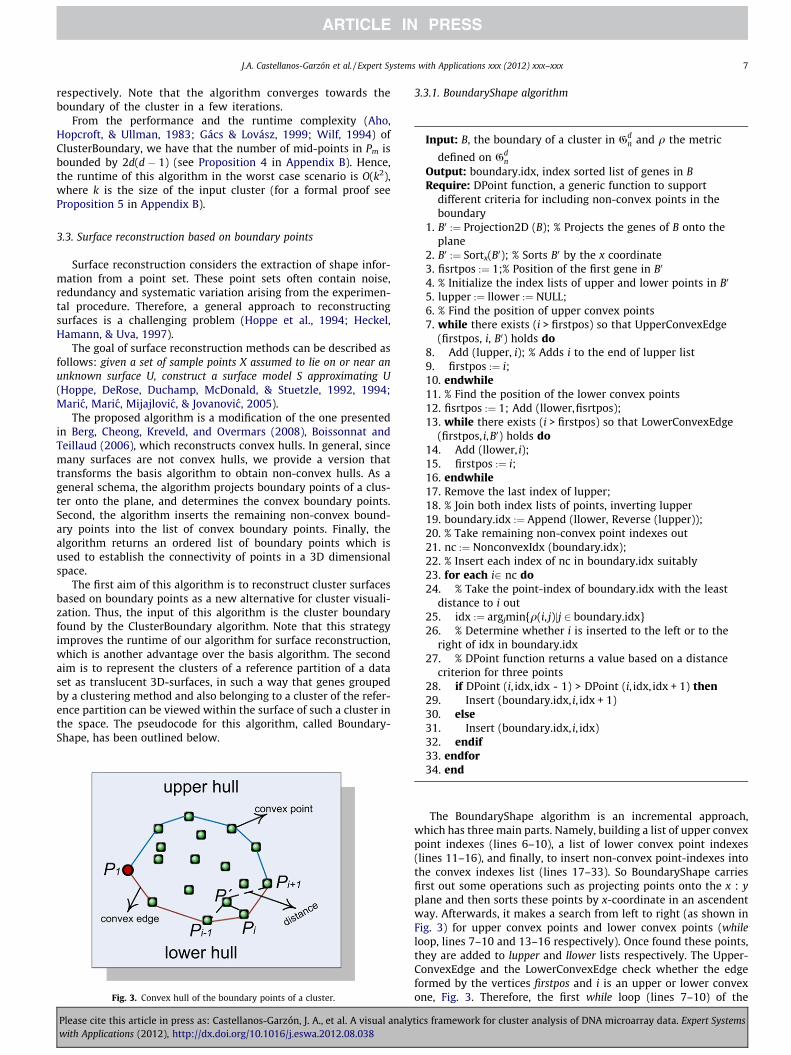
Fig. 3. Convex hull of the boundary points of a cluster.


3.3.1. BoundaryShape algorithm

Input: B, the boundary of a cluster in Gdn and q the metric

defined on Gdn

Output: boundary.idx, index sorted list of genes in BRequire: DPoint function, a generic function to support

different criteria for including non-convex points in theboundary

1. B0 :¼ Projection2D (B); % Projects the genes of B onto theplane

2. B0 :¼ Sortx(B0); % Sorts B0 by the x coordinate3. fisrtpos :¼ 1;% Position of the first gene in B0

4. % Initialize the index lists of upper and lower points in B0

5. lupper :¼ llower :¼ NULL;6. % Find the position of upper convex points7. while there exists (i > firstpos) so that UpperConvexEdge

(firstpos, i, B0) holds do8. Add (lupper, i); % Adds i to the end of lupper list9. firstpos :¼ i;10. endwhile11. % Find the position of the lower convex points12. fisrtpos :¼ 1; Add (llower,fisrtpos);13. while there exists (i > firstpos) so that LowerConvexEdge

(firstpos, i,B0) holds do14. Add (llower, i);15. firstpos :¼ i;16. endwhile17. Remove the last index of lupper;18. % Join both index lists of points, inverting lupper19. boundary.idx :¼ Append (llower, Reverse (lupper));20. % Take remaining non-convex point indexes out21. nc :¼ NonconvexIdx (boundary.idx);22. % Insert each index of nc in boundary.idx suitably23. for each i2 nc do24. % Take the point-index of boundary.idx with the least

distance to i out25. idx :¼ argjmin{q(i, j)jj 2 boundary.idx}26. % Determine whether i is inserted to the left or to the

right of idx in boundary.idx27. % DPoint function returns a value based on a distance

criterion for three points28. if DPoint (i, idx, idx - 1) > DPoint (i, idx, idx + 1) then29. Insert (boundary.idx, i, idx + 1)30. else31. Insert (boundary.idx, i, idx)32. endif33. endfor34. end

The BoundaryShape algorithm is an incremental approach,which has three main parts. Namely, building a list of upper convexpoint indexes (lines 6–10), a list of lower convex point indexes(lines 11–16), and finally, to insert non-convex point-indexes intothe convex indexes list (lines 17–33). So BoundaryShape carriesfirst out some operations such as projecting points onto the x : yplane and then sorts these points by x-coordinate in an ascendentway. Afterwards, it makes a search from left to right (as shown inFig. 3) for upper convex points and lower convex points (whileloop, lines 7–10 and 13–16 respectively). Once found these points,they are added to lupper and llower lists respectively. The Upper-ConvexEdge and the LowerConvexEdge check whether the edgeformed by the vertices firstpos and i is an upper or lower convexone, Fig. 3. Therefore, the first while loop (lines 7–10) of the




algorithm computes only those convex hull vertices that lie on theupper hull (blue edges in Fig. 3). That is, the part of the convex hullrunning from the leftmost point P1 to the rightmost point Pi+1,when the points are listed clockwise order as shown in Fig. 3.The second while loop (lines 13–16) does the same but for verticesthat lie on the lower hull (red edges).

At the end of the algorithm, boundary.idx is formed by joiningllower and the reverse of lupper, which allows the convex points tobe stored in anti-clockwise order. The set nc stores the remainingnon-convex points that are finally inserted into boundary.idx inthe for loop (lines 23–33). The value of idx in this loop is the pointnearest to i (the convex point closest to P0 in Fig. 3 is Pi). We thenhave to decide whether i is inserted to the left or the right of idx,which is done using DPoint. DPoint is a generic function that canuse a number of distance criteria as shown in Fig. 3. Briefly, thepoint P0 (Fig. 3) can be inserted to the left or right of Pi basedon the smaller of the distances between (P0,Pi�1) and (P0,Pi+1),the smaller of the distances from P0 to the edges (Pi, Pi�1) and (Pi, -Pi+1), the shorter of the paths connecting (P0,Pi�1,Pi) and (P0,Pi+1,Pi),or the smaller of the areas DP0Pi�1Pi and DP0Piþ1Pi. Note that, inthis figure, P0 should be inserted to the left of Pi (the area ofDP0Pi�1Pi is less than the area of DP0Piþ1Pi), implying that the edge(Pi,Pi�1) is replaced by the edges (P0,Pi�1) and (P0,Pi). This mecha-nism allows a convex boundary to become non-convex (see alsoFig. 2d2).

The information given by the output of the BoundaryShapealgorithm is used for the 3D triangulation of the surface that

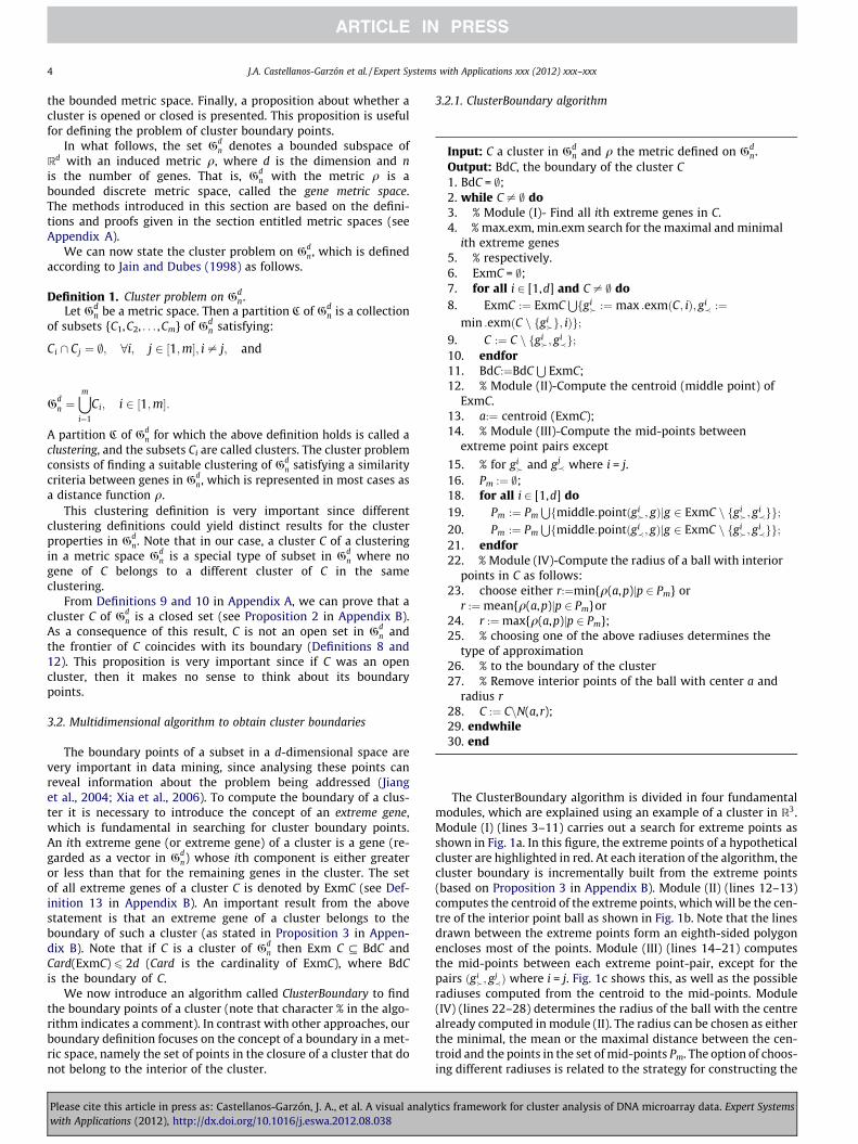
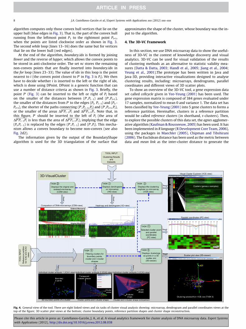
Fig. 4. General view of the tool. There are eight linked views and six tasks of cluster visutop of the figure; 3D scatter plot views at the bottom; cluster boundary points, referenc


approximates the shape of the cluster, whose boundary was the in-put to the algorithm.

4. The 3D-VC Framework

In this section, we use DNA microarray data to show the useful-ness of 3D-VC in the context of knowledge discovery and visualanalytics. 3D-VC can be used for visual validation of the resultsof clustering methods as an alternative to statistic validity mea-sures (Datta & Datta, 2003; Handl et al., 2005; Jiang et al., 2004;Yeung et al., 2001).The prototype has been written in Java andJava-3D, providing interactive visualizations designed to analyseclustering results, including: microarrays, dendrograms, parallelcoordinates and different views of 3D scatter plots.

To show an overview of the 3D-VC tool, a gene expression dataset called cellcycle given in Yee-Yeung (2001) has been used. Thegene expression matrix is composed of 384 genes evaluated under17 samples, normalized to mean 0 and variance 1. The data set hasbeen classified by Yee-Yeung (2001) into 5 gene clusters to forms areference partition. Hereinafter, clusters in a reference partitionwould be called reference clusters (in shorthand, r-clusters). Then,to explore the possible clusters of this data set, the agnes agglomer-ative algorithm (Kaufman & Rousseeuw, 2005) has been used. It hasbeen implemented in R language (R Development Core Team, 2006),using the packages in Maechler (2005), Chipman and Tibshirani(2006). The Euclidean distance has been used as the metric betweendata and mean link as the inter-cluster distance to generate the

al analysis showing: microarray, dendrogram and parallel coordinates views at thee partition shapes and cluster shape reconstruction.



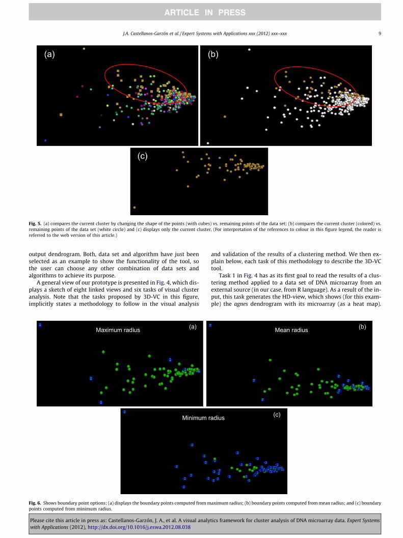
Fig. 5. (a) compares the current cluster by changing the shape of the points (with cubes) vs. remaining points of the data set; (b) compares the current cluster (colored) vs.remaining points of the data set (white circle) and (c) displays only the current cluster. (For interpretation of the references to colour in this figure legend, the reader isreferred to the web version of this article.)


output dendrogram. Both, data set and algorithm have just beenselected as an example to show the functionality of the tool, sothe user can choose any other combination of data sets andalgorithms to achieve its purpose.

A general view of our prototype is presented in Fig. 4, which dis-plays a sketch of eight linked views and six tasks of visual clusteranalysis. Note that the tasks proposed by 3D-VC in this figure,implicitly states a methodology to follow in the visual analysis

Fig. 6. Shows boundary point options; (a) displays the boundary points computed from mpoints computed from minimum radius.


and validation of the results of a clustering method. We then ex-plain below, each task of this methodology to describe the 3D-VCtool.

Task 1 in Fig. 4 has as its first goal to read the results of a clus-tering method applied to a data set of DNA microarray from anexternal source (in our case, from R language). As a result of the in-put, this task generates the HD-view, which shows (for this exam-ple) the agnes dendrogram with its microarray (as a heat map).

aximum radius; (b) boundary points computed from mean radius; and (c) boundary



Table 2Comparative table of agreement and disagreement of clustering results with respect to the reference partition of cellcycle.

Method Case #Clusters Agreement DisagreementMM

JC RI ARI

Agnes 0.20615 0.39175 �0.00455 1.63176Diana A 5 0.20957 0.38518 �0.00048 1.64056

Eisen 0.22690 0.24387 �0.00153 1.81936

Agnes 0.16953 0.56706 0.00485 1.37668Diana B 13 0.13083 0.65473 0.00810 1.22939Eisen 0.20719 0.39583 �0.00157 1.62622


This view provides an overall analysis of the whole clustering pro-cess. The second goal of Task 1 is to generate from the input, twonew tasks, 2 and 3, which give way to a new analysis on differentviews. For its part, Task 2 in Fig. 4 has as a goal to compare the ori-ginal and the ordered microarray according to the applied cluster-ing method using the CDM-view. Genes in a cluster on the orderedmicroarray can also be located on the original microarray (throughthe red lines between both microarrays). This task is optional in theanalysis process and is also useful to compare several clusteringmethods according to the reordering applied by them to the origi-nal microarray.

On the order hand, a continuation of Task 1 is Task 3, which hasas a goal to locally explore the clusterings (and clusters) of the den-drogram shown by Task 1, through the result given by the VCE-view. Every level (clustering) of the dendrogram can be chosen

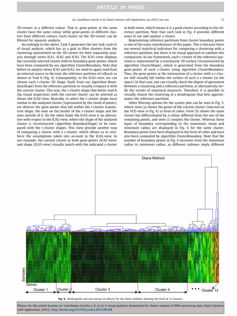
Fig. 7. Dendrogram and microarray of cellcycle for Agnes method, showin


on the left side in the VCE-view, and the clusters of the chosen levelare shown on the right side. Therefore, this view explores in detaileach cluster in the dendrogram and moreover, it is a new visual aidfor exploring clusters on the microarray.

From Task 3, two possible tasks, Tasks 4 and 5, can be followed.Task 4 has as a goal to carry out a zoom-in of the selected cluster inthe VCE-view and show it as a result by including parallel coordi-nates in the PC-view. Parallel coordinates are added for each sam-ple of genes in the cluster, providing a means of comparison of thecluster quality. Task 5 has as a goal to give a different visualizationalternative from the VCE-view. In this case, the clustering selectedin the VCE-view (Task 3) has been shown in form of a 3D scatterplot by applying PCA (through the covariance matrix) to reducethe gene space dimensionality to obtain the view of the 3D-viewer.Each cluster in the current clustering has been displayed on the

g the level of 13 clusters. Clusters are enumerated from left to right.




3D-viewer in a different colour. That is, gene-points in the samecluster have the same colour while gene-points in different clus-ters have different colours. Each cluster on the 3D-viewer can befiltered for separate analysis.

Accordingly to the above, Task 5 generates the last task (task 6)of visual analysis, which has as a goal to filter clusters from theclustering represented on the 3D-viewer for their separately anal-ysis through views ICA1, ICA2 and ICA3. The ICA1-view displaysthe currently selected cluster with its boundary gene-points, whichhave been computed by our algorithm ClusterBoundary. Note thatbefore to analyse views ICA2 and ICA3, we need to again read froman external source to the tool, the reference partition of cellcycle asshown in Task 6 (Fig. 4). Consequently, in the ICA2-view, we canchoose each r-cluster 3D shape (built from our algorithm Boun-daryShape) from the reference partition to visually compare it withthe current cluster. This way, the r-cluster shape that better match(by visual inspection) with the current cluster can be selected asshows the ICA2-view. Basically, to select the r-cluster shape mostsimilar to the analysed cluster (represented by the cloud of points),we observe the gene-points that fall within the r-cluster translu-cent shape, the ones on the border of the r-cluster shape and theones outside of it. On the other hand, the ICA3-view is an alterna-tive with respect to the ICA2-view, where the shape of the analysedcluster is reconstructed (algorithm BoundaryShape) to be com-pared with the r-cluster shapes. This view provide another wayof comparing a cluster with a r-cluster, which allows us to rein-force the assumptions taken into account in the ICA2-view. Inour example, the current cluster as both gene-points (ICA2-view)and shape (ICA3-view) visually match with the indicated r-cluster

Fig. 8. Dendrogram and microarray of cellcycle for the


in both views, which means it is a good cluster according to the ref-erence partition. Note that each task in Fig. 4 provides differentways to see and analyse a cluster.

Representing reference partitions from cluster boundary pointsis one of the main contributions of this paper. This is because thereare several statistical indicators for comparing a clustering with areference partition, but there is no visual approach to validate thiscomparison. In our framework, each r-cluster of the reference par-tition is represented by a translucent 3D surface (reconstructed byalgorithm ClusterShape), which is generated from the boundarygene-points of each r-cluster using algorithm ClusterBoundary.Thus, the gene-points at the intersection of a cluster with a r-clus-ter will visually fall within the surface of such a r-cluster (in thespace). In that case, one can visually check the degree of agreementbetween a clustering and a reference partition, or alternatively ver-ify the results of statistical measures. Therefore, it is possible tovisually choose the clustering of a dendrogram that best approxi-mates the reference partition.

Other filtering options for the scatter plot can be seen in Fig. 5,where view (a) shows the genes of the current cluster (selected onthe VCE-view in Fig. 4) in form of cubes. View (b) shows the samecluster but differentiated by a colour different from the one of theremaining points, and view (c) isolates the cluster. Whereas threetypes of boundary corresponding to the maximum, mean andminimum radius are displayed in Fig. 6 for the same cluster.Boundary points have been displayed in the form of cubes and havealso been computed by algorithm ClusterBoundary. Note that thenumber of boundary points in Fig. 6 increases from the maximumradius to minimum radius, as different radiuses imply different

Diana method, showing the level of 13 clusters.




approximations of the cluster boundary. The radius determines thenumber of interior points to be removed from a cluster. Thus, theuser can choose the type of boundary according to the application.That is, the maximum radius is more suitable to represent 3Dsurfaces of r-clusters, whereas a smaller radius may be more suit-able to represent clusters by their boundary points (or their shapes).

5. A Case Study

This section presents a case study of the cellcycle data set (Yee-Yeung, 2001) and its reference partition of 5 r-clusters. The goal ofthis case study is to show that the visual validation and the numer-ical validation (cluster validity measures) of the results from theclustering methods are consistent with respect to a reference par-tition of the given data set. Note that not always visual validationmatches the numerical validation, since the numerical validationsare based on different assumptions. Then, to reach the previousgoal, we first compare the results of three clustering methods withthe reference partition for cellcycle by mean of statistical indicesthat measure the similarity degree. Afterwards, we also visuallycompare the quality of the used statistical indices and show therelationships (numerical and visual) between the reference parti-tion and the clustering results.

To this end, the hierarchical clustering methods Agnes and Dia-na from Kaufman and Rousseeuw (2005) and Eisen from Eisen et al.(1998), are applied to cellcycle. The following statistical indices areused: the Rand index (RI), the Jaccard coefficient (JC), the Minkow-ski measure (MM) (Halkidi, Batistakis, & Vazirgiannis, 2001; Sokal,

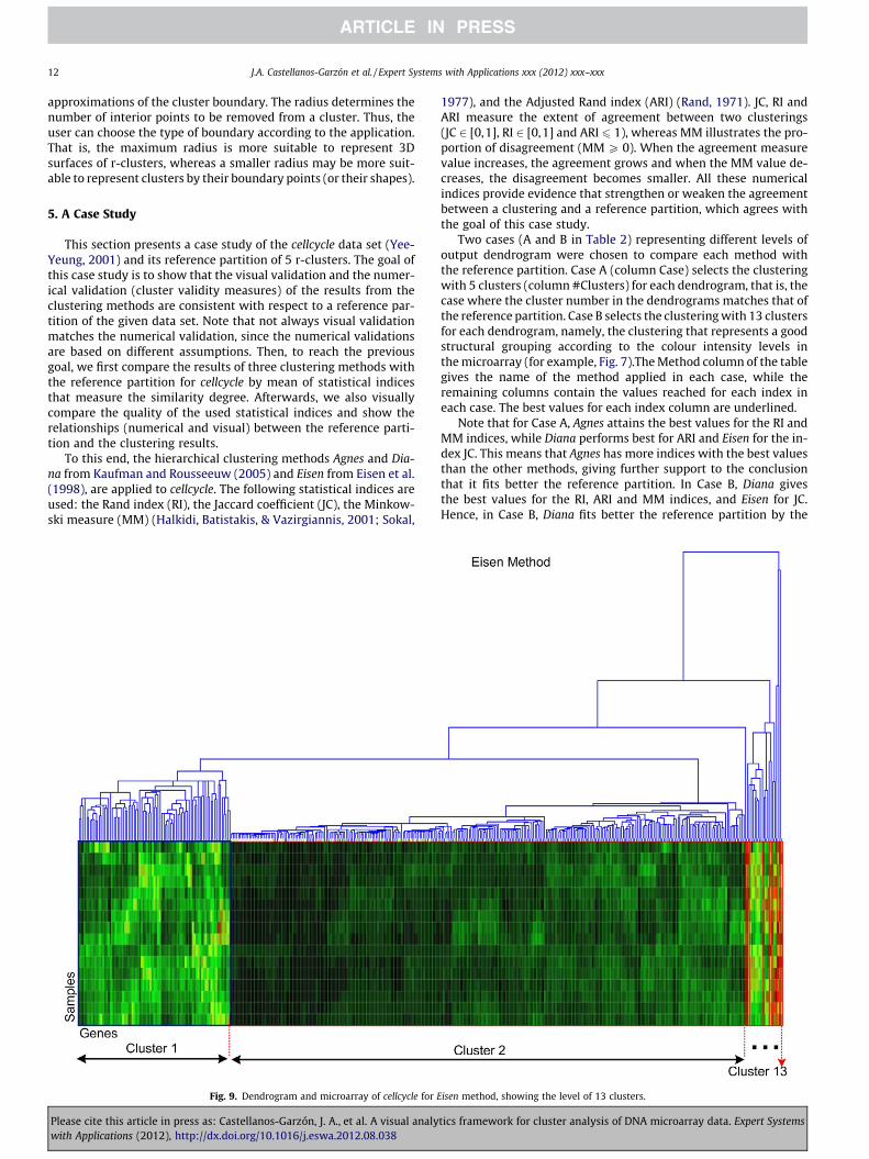
Fig. 9. Dendrogram and microarray of cellcycle for E


1977), and the Adjusted Rand index (ARI) (Rand, 1971). JC, RI andARI measure the extent of agreement between two clusterings(JC 2 [0,1], RI 2 [0,1] and ARI 6 1), whereas MM illustrates the pro-portion of disagreement (MM P 0). When the agreement measurevalue increases, the agreement grows and when the MM value de-creases, the disagreement becomes smaller. All these numericalindices provide evidence that strengthen or weaken the agreementbetween a clustering and a reference partition, which agrees withthe goal of this case study.

Two cases (A and B in Table 2) representing different levels ofoutput dendrogram were chosen to compare each method withthe reference partition. Case A (column Case) selects the clusteringwith 5 clusters (column #Clusters) for each dendrogram, that is, thecase where the cluster number in the dendrograms matches that ofthe reference partition. Case B selects the clustering with 13 clustersfor each dendrogram, namely, the clustering that represents a goodstructural grouping according to the colour intensity levels inthe microarray (for example, Fig. 7).The Method column of the tablegives the name of the method applied in each case, while theremaining columns contain the values reached for each index ineach case. The best values for each index column are underlined.

Note that for Case A, Agnes attains the best values for the RI andMM indices, while Diana performs best for ARI and Eisen for the in-dex JC. This means that Agnes has more indices with the best valuesthan the other methods, giving further support to the conclusionthat it fits better the reference partition. In Case B, Diana givesthe best values for the RI, ARI and MM indices, and Eisen for JC.Hence, in Case B, Diana fits better the reference partition by the

isen method, showing the level of 13 clusters.



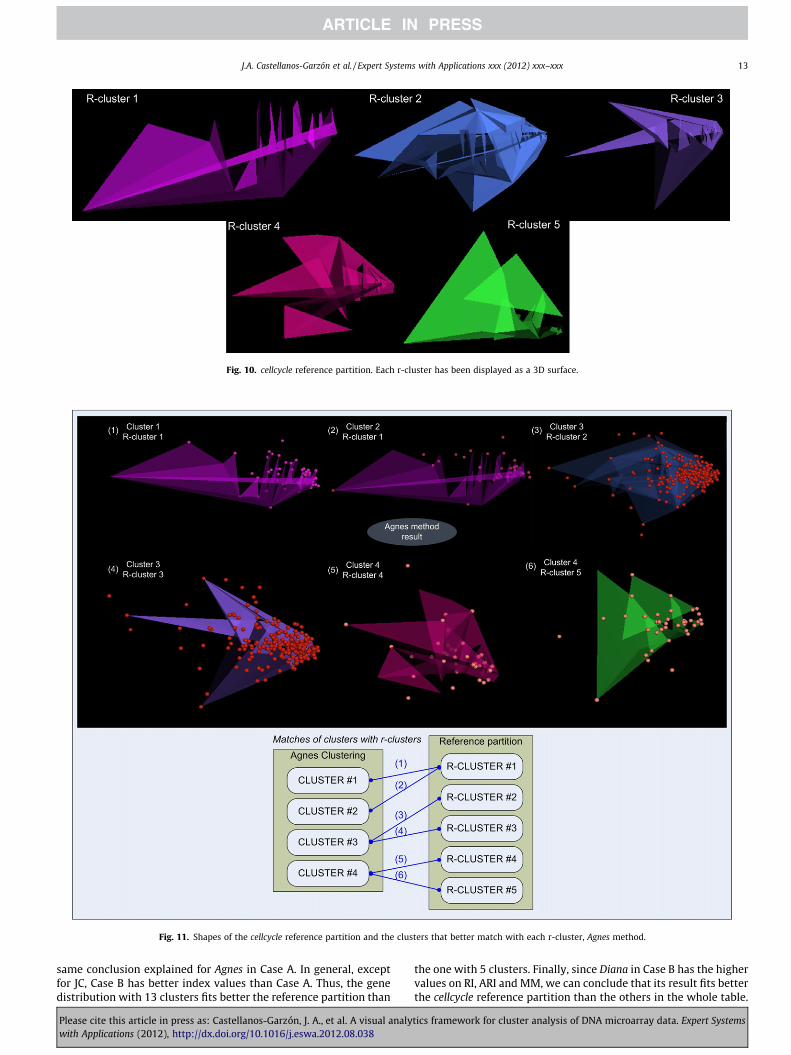
Fig. 10. cellcycle reference partition. Each r-cluster has been displayed as a 3D surface.

Fig. 11. Shapes of the cellcycle reference partition and the clusters that better match with each r-cluster, Agnes method.


same conclusion explained for Agnes in Case A. In general, exceptfor JC, Case B has better index values than Case A. Thus, the genedistribution with 13 clusters fits better the reference partition than


the one with 5 clusters. Finally, since Diana in Case B has the highervalues on RI, ARI and MM, we can conclude that its result fits betterthe cellcycle reference partition than the others in the whole table.




5.1. Visual Check of the Results

As the final part of the case study, we now check that the indexresults for Case B correspond to the visual representation of themicroarray view and with the reference partition of cellcycle inthe scatter plot view. This allows us a validation process of allthe used indices. Firstly, we show the microarray and dendrogramview for each method in Case B in Table 2 by Figs. 7–9, which verifythat Diana finds a better gene cluster distribution than the othermethods. That is, through a visual comparison of the clusters withsimilar colours, marked on the heat map (red rectangles) in thoseFigs. 7–9, we can see Diana has better division of clusters thanAgnes and Eisen. In contrast, Eisen (Fig. 9) shows the worst divisionof clusters on the heat map.

Secondly, we visually compare the clustering of each method inCase B against the reference partition, aimed at finding the methodthat yields the clustering most in agreement with the referencepartition. A visual representation of the cellcycle reference partitionis given by Fig. 10, which shows the 3D-surfaces of its five r-clus-ters, computed from the ClusterShape algorithm. In order to com-pare the r-clusters with the clusters in Case B in Table 2, a visualinspection has been carried out for the clusters of each methodsimilar to these r-cluster shapes.

Figs. 11–13 show the r-clusters (in the form of 3D-surfaces)overlapped on the clusters (represented as a cloud of gene-points)most similar to them for each method of Case B in Table 2. ForAgnes in Fig. 11, six visual matches have visually been found foronly four clusters with respect to the reference partition. Theremaining clusters for Agnes are not considered because they arevery small and so match with any r-cluster. The process followed

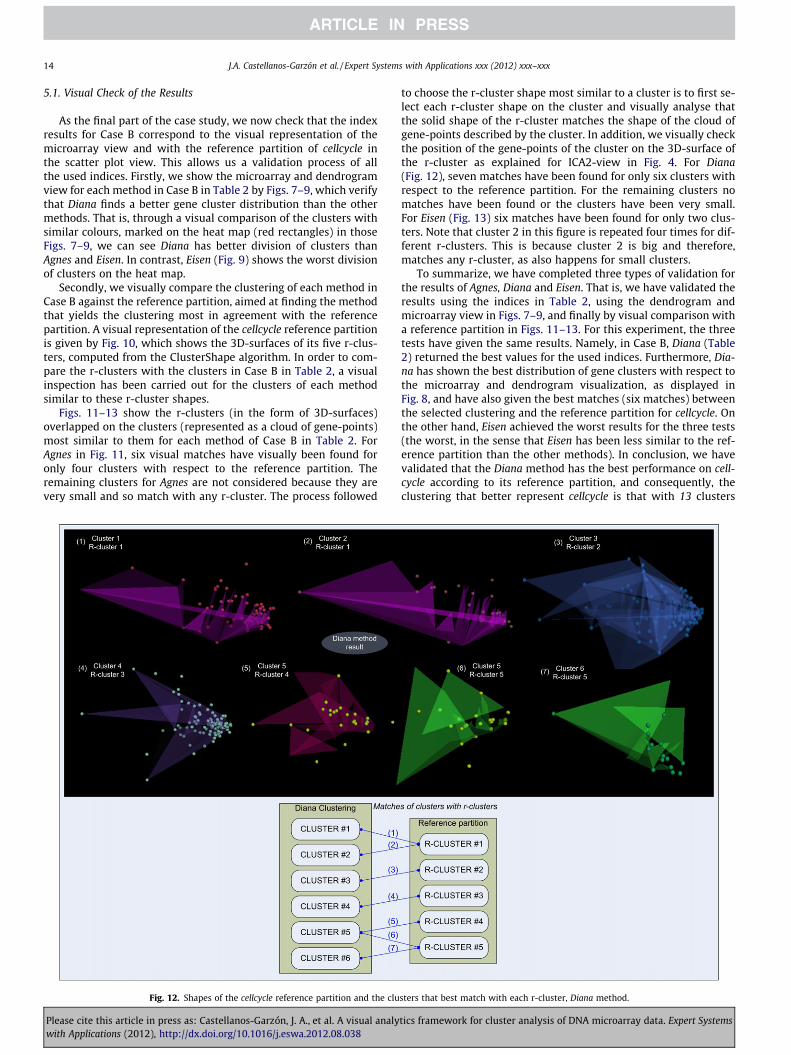
Fig. 12. Shapes of the cellcycle reference partition and the clu


to choose the r-cluster shape most similar to a cluster is to first se-lect each r-cluster shape on the cluster and visually analyse thatthe solid shape of the r-cluster matches the shape of the cloud ofgene-points described by the cluster. In addition, we visually checkthe position of the gene-points of the cluster on the 3D-surface ofthe r-cluster as explained for ICA2-view in Fig. 4. For Diana(Fig. 12), seven matches have been found for only six clusters withrespect to the reference partition. For the remaining clusters nomatches have been found or the clusters have been very small.For Eisen (Fig. 13) six matches have been found for only two clus-ters. Note that cluster 2 in this figure is repeated four times for dif-ferent r-clusters. This is because cluster 2 is big and therefore,matches any r-cluster, as also happens for small clusters.

To summarize, we have completed three types of validation forthe results of Agnes, Diana and Eisen. That is, we have validated theresults using the indices in Table 2, using the dendrogram andmicroarray view in Figs. 7–9, and finally by visual comparison witha reference partition in Figs. 11–13. For this experiment, the threetests have given the same results. Namely, in Case B, Diana (Table2) returned the best values for the used indices. Furthermore, Dia-na has shown the best distribution of gene clusters with respect tothe microarray and dendrogram visualization, as displayed inFig. 8, and have also given the best matches (six matches) betweenthe selected clustering and the reference partition for cellcycle. Onthe other hand, Eisen achieved the worst results for the three tests(the worst, in the sense that Eisen has been less similar to the ref-erence partition than the other methods). In conclusion, we havevalidated that the Diana method has the best performance on cell-cycle according to its reference partition, and consequently, theclustering that better represent cellcycle is that with 13 clusters

sters that best match with each r-cluster, Diana method.



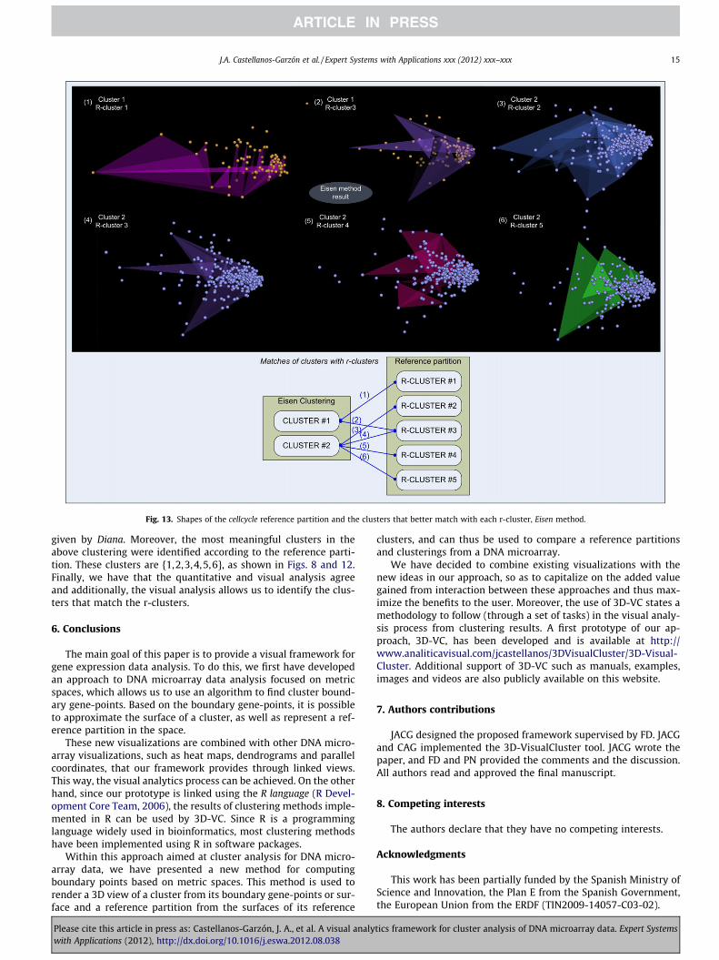
Fig. 13. Shapes of the cellcycle reference partition and the clusters that better match with each r-cluster, Eisen method.


given by Diana. Moreover, the most meaningful clusters in theabove clustering were identified according to the reference parti-tion. These clusters are {1,2,3,4,5,6}, as shown in Figs. 8 and 12.Finally, we have that the quantitative and visual analysis agreeand additionally, the visual analysis allows us to identify the clus-ters that match the r-clusters.

6. Conclusions

The main goal of this paper is to provide a visual framework forgene expression data analysis. To do this, we first have developedan approach to DNA microarray data analysis focused on metricspaces, which allows us to use an algorithm to find cluster bound-ary gene-points. Based on the boundary gene-points, it is possibleto approximate the surface of a cluster, as well as represent a ref-erence partition in the space.

These new visualizations are combined with other DNA micro-array visualizations, such as heat maps, dendrograms and parallelcoordinates, that our framework provides through linked views.This way, the visual analytics process can be achieved. On the otherhand, since our prototype is linked using the R language (R Devel-opment Core Team, 2006), the results of clustering methods imple-mented in R can be used by 3D-VC. Since R is a programminglanguage widely used in bioinformatics, most clustering methodshave been implemented using R in software packages.

Within this approach aimed at cluster analysis for DNA micro-array data, we have presented a new method for computingboundary points based on metric spaces. This method is used torender a 3D view of a cluster from its boundary gene-points or sur-face and a reference partition from the surfaces of its reference


clusters, and can thus be used to compare a reference partitionsand clusterings from a DNA microarray.

We have decided to combine existing visualizations with thenew ideas in our approach, so as to capitalize on the added valuegained from interaction between these approaches and thus max-imize the benefits to the user. Moreover, the use of 3D-VC states amethodology to follow (through a set of tasks) in the visual analy-sis process from clustering results. A first prototype of our ap-proach, 3D-VC, has been developed and is available at http://www.analiticavisual.com/jcastellanos/3DVisualCluster/3D-Visual-Cluster. Additional support of 3D-VC such as manuals, examples,images and videos are also publicly available on this website.

7. Authors contributions

JACG designed the proposed framework supervised by FD. JACGand CAG implemented the 3D-VisualCluster tool. JACG wrote thepaper, and FD and PN provided the comments and the discussion.All authors read and approved the final manuscript.

8. Competing interests

The authors declare that they have no competing interests.

Acknowledgments

This work has been partially funded by the Spanish Ministry ofScience and Innovation, the Plan E from the Spanish Government,the European Union from the ERDF (TIN2009-14057-C03-02).







Appendix A. Metric spaces

Definition 2 (Metric spaces). If E is an arbitrary set andq : E E! R a mapping called the distance, then the pair hE,qi(abbreviated to E) is a metric space if q is a metric defined on E.That is, for all points x, y, z 2 E, the following are satisfied:

1. Positiveness: q(x,y) > 0 if x – y, and q(x,x) = 0.2. Symmetry: q(x,y) = q(y,x).3. Triangle inequality: q(x,z) 6 q(x,y) + q(y,z).

Definition 3 (Bounded metric spaces). Let E be a metric space con-sisting with the metric q. If there exists a positive number k suchthat q(x,y) 6 k for all points x, y 2 E, then we say that E is a boundedmetric space.

Definition 4 (Diameter of a subset of a metric space). Let A be a sub-set of a metric space E. Consider the set of non-negative real num-bers {q(x,y)jx 2 A,y 2 A}. If this set is bounded, then it hassupremum, denoted d(A), which is called the diameter of A.

Definition 5 (Distance between two subsets). Let A and B be twosubsets of a metric space E. The set of real numbers{q(x,y)jx 2 A,y 2 B}, is bounded below by zero. Its infimum,denoted by q(A,B), is called the distance between A and B.

In the case that A and B can be considered as clusters, other defi-nitions of distance between them can be given (Jain & Dubes, 1998).

Definition 6 (Subspace of a metric space). Let E be a metric spacewith the metric q, and let E0 be a proper subset of E. Let q0 be therestriction of q to E0 E0, so that q0(x,y) = q(x,y) for all x and y in E0.Then q0 is called an induced metric and E0 with the metric q0 iscalled a subspace of E.

The gene expression matrix (m n) of a DNA microarray can beviewed as a subspace of Rn (see Proposition 1).

Definition 7 (Balls). If a is a point in a metric space E with themetric q, then the set of all points x 2 E such that q(a,x) < r, wherer > 0, is called a ball (or neighborhood) of centre a and radius r, andis denoted by N(a,r).

Definition 8 (Open sets). If A is a subset in a metric space E, thepoint a 2 A is said to be an interior point of A if it is the centre ofa ball which consists only of points in A. The set of all interiorpoints of A (IntA) is called the interior of A. If every point of A isinterior, then A is called an open set.

Definition 9 (Adherent points). If A is a subset of a metric space E,the point a 2 E is said to be an adherent point of A if every ball withcentre a contains a point of A.

Definition 10 (Closure). If A is a subset of a metric space E, the clo-sure of A, denoted by A, is the set of all adherent points of A. Clearly,A A. If A ¼ A, we say that A is closed.

Definition 11 (Exterior points). A point is said to be an exteriorpoint of A if it is an interior point of the complement Ac. The exte-rior of A (Ext A) is the set of all exterior points of A.

Definition 12. (Frontier points). The set A \ Ac , which isnot necessar-ily empty, is called the frontier of A, denoted FrA. The boundary of a setA, denoted BdA, is the part of the frontier of A which belongs to A.


Appendix B. Theoretical results

Proposition 1 (Gene subspace). Consider the metric space Rd andwithout loose of generality, the Euclidean distance q0 defined on Rd.Let Xnd be a gene expression matrix of DNA microarray data, andlet G

dn be a set consisting of all row points (genes) in Xnd. Then G

dn

is a bounded subspace of Rd with the induced metric q withq(gx,gy) = q0(gx,gy), for gx and gy genes in G

dn.

Proof. This proposition can be verified from Definitions 2, 3 and 6in Appendix A. h

Proposition 2. (Closed cluster). If Gdn is a gene metric space with a

metric q, then every cluster C of Gdn is a closed set (closed cluster) in G

dn.

Proof. From Definitions 9 and 10, it is necessary to prove that C ¼ C.We do this by reductio ad absurdum. Suppose that x 2 G

dn is an exterior

gene of C (see Definition 11) that is also an adherent gene of C. Thenx 2 C and C – C, and moreover,8r 2 R; 9a 2 C; a 2 Nðx; rÞ (see Defini-tion 7). If, in particular, r = q(x,C)/2 (see Definition 5), then 9= a 2 C suchthat a 2 N(x,q(x,C)/2), and so x R C, which is a contradiction to ourprevious assumption. Hence, x 2 C, C ¼ C and thus C is closed. h

Definition 13 (Extreme gene). Let C be a cluster of a gene metricspace G

dn. A gene g 2 C such that g = (x1,x2, . . . ,xi, . . . ,xd) is said to

be an ith extreme gene (or an extreme gene) of C, i 2 [1,d], if eitherxi P x0i or xi 6 x0i8g0 ¼ ðx01; x02; . . . ; x0i; . . . ; x0dÞ 2 C n fgg. An ith extremegene g 2 C is denoted as gi

� when xi P x0i or gi� when xi < x0i in the

above mentioned condition. The set of all extreme genes of C isdenoted by ExmC.

Proposition 3 (Extreme genes and cluster boundary). Ifg = (x1,x2, . . . , xi, . . . , xd) is an ith extreme gene of a cluster C of G

dn,

then g 2 BdC.

Proof. It is enough to prove that g 2 C is not an interior gene of C.This is true because in any ball N(g,r) with r > 0, we can find a geneg0 ¼ ðx01; x02; . . . ; x0i; . . . ; x0dÞ with either x0i > xi or x0i < xi (according tothe case) such that g0 is an ith extreme gene of C [ {g0} andq(g0,g) < r, i 2 [1,d]. This implies that g0 2 N(g,r) and g0 R C, so g isnot an interior gene in C and hence g 2 Bd C. h

Proposition 4 (Cardinality of Pm). Since Pm is the set of mid-points,where 2d extreme points are achieved from an iteration of Cluster-Boundary, the cardinality of Pm is Card(Pm) = 2d(d � 1).

Proof. The number of mid-points computed from extreme points,and that satisfy module (III) of the algorithm, can be expressed as4Pd�1

i¼1 ðd� iÞ. Expanding this expression, the required result isreached. h

Proposition 5 (Runtime of ClusterBoundary). The temporal com-plexity of ClusterBoundary for computing the cluster boundary in agene metric space G

dn is O(k2), where k is the size of the cluster.

Proof. Module (I) of this algorithm can run in d k steps, and eachof the other modules can run in d2 steps. The above results are pro-ven directly for modules (I) and (II), while for modules (III) and (IV)the proof uses Proposition 4. Hence, the order of one iteration ofthe algorithm is O(k d). On the other hand, the number of itera-tions performed by the algorithm satisfies the inequalityk � (i � 1)d P 0, where i is the number of iterations. Solving thisinequality, we observe that the number of iterations is boundedby k

dþ 1 and so, the order of ClusterBoundary is O(k2). h




References

Aho, A. V., Hopcroft, J. E., & Ullman, J. D. (1983). Data structures and algorithms.Reading, Massachusetts: Addison-Wesley.

Alon, U., Barkai, N., Notterman, D. A., Gish, K., Ybarra, S., Mack, D., et al. (1999).Broad patterns of gene expression revealed by clustering analysis of tumor andnormal colon tissues probed by oligonucleotide arrays. Proceedings of theNational Academy of Sciences, USA, 96, 6745–6750.

Baldin, P., & Brunak, S. (1998). Bioinformatics: The machine learning approach.Cambridge, MA: MIT Press.

Belacel, N., Wang, Q., & Cuperlovic-Culf, M. (2006). Clustering methods formicroarray gene expression data. OMICS: A Journal of Integrative Biology, 10(4),507–531. A special issue on current microarray research.

Berg, M. d., Cheong, O., Kreveld, M. v., & Overmars, M. (2008). Computationalgeometry, algorithms and applications (Third ed.). Berlin, Heidelberg: Springer-Verlag. ISBN 978-3-540-77973-5.

Berrar, D. P., Dubitzky, W., & Granzow, M. (2003). A practical approach to microarraydata analysis. New York, Boston, Dordrecht, London, Moscow: Kluwer AcademicPublishers..

Boissonnat, J. D., & Teillaud, M. (2006). Mathematics and visualization. Berlin,Heidelberg: Springer-Verlag.

Chan, Z. S. H., & Kasabov, N. (2004). Gene trajectory clustering with a hybrid geneticalgorithm and expectation maximization method. In IEEE international jointconference on neural networks, Vol. 3, pp. 1669–1674.

Chipman, H., & Tibshirani, R. (2006). with tsvq code originally from Trevor Hastie,hybridHclust: Hybrid hierarchical clustering, R package version 1.0-1. <http://ace.acadiau.ca/math/chipmanh/hybridHclust>.

Datta, S., & Datta, S. (2003). Comparisons and validation of statistical clusteringtechniques for microarray gene expression data. Bioinformatics (Vol. 19,pp. 459–465). Datta2003.

Dhaeseleer, P., Wen, X., Fuhrman, S., & Somogyi, R. (1998). Mining the geneexpression matrix: Inferring gene relationships from large scale geneexpression data. Information Processing in Cells and Tissues, 203–212.

Duda, R. O., Hart, P. E., & Stork, D. G. (2001). Pattern classification (2nd ed.). NewYork: Wiley.

Eisen, M., Spellman, T., Brown, P., & Botstein, D. (1998). Cluster analysis and displayof genome-wide expression patterns. Proceedings of the National Academy ofSciences, USA, 95, 14863–14868.

Eisen, M. B. (2002). Cluster 2.20 and treeview 1.60, Eisen Lab. <http://rana.lbl.gov/EisenSoftware.htm>.

Gács, P., & Lovász, L. (1999). Complexity of algorithms. In Lecture notes. Berlin,Heidelberg: Springer-Verlag.

Geoffrey, J. M., Do, K. A., & Ambroise, C. (2004). Analyzing microarray gene expressiondata. Hoboken, New Jersey: John Wiley & Sons Inc..

Halkidi, M., Batistakis, Y., & Vazirgiannis, M. (2001). On clustering validationtechniques. Intelligent Information Systems Journal.

Handl, J., Knowles, J., & Kell, D. B. (2005). Computational cluster validation in post-genomic data analysis. Oxford University Press. Vol. 21, pp. 3201–3212.

Han, J., & Kamber, M. (2006). Data mining: Concepts and techniques. Elsevier Inc..Heckel, B., Hamann, B., & Uva, A. E. (1997). Cluster-based generation of hierarchical

surface models. In Scientific visualization conference (pp. 105–114). IEEEComputer Societyhttp://doi.ieeecomputersociety.org/10.1109/DAGSTUHL.1997.10036 .

Hoppe, H. (1994). Surface reconstruction from unorganized points. Ph.D. thesis,University of Washington, Department of Computer Science and Engineering.

Hoppe, H., DeRose, T., Duchamp, T., McDonald, J., & Stuetzle, W. (1992). Surfacereconstruction from unorganized points. In SIGGRAPH ’92: Proceedings of the19th annual conference on Computer graphics and interactive techniques (pp. 71–78), ACM, New York, NY, USA. http://dx.doi.org/10.1145/133994.134011.

Hoppe, H., DeRose, T., Duchamp, T., Halstead, M., Jin, H., McDonald, J., Schweitzer, J.,& Stuetzle, W. (1994). Piecewise smooth surface reconstruction. In SIGGRAPH’94: Proceedings of the 21st annual conference on Computer graphics andinteractive techniques (pp. 295–302) ACM, New York, NY, USA. http://dx.doi.org/10.1145/192161.192233.

Inselberg, A., & Dimsdale, B. (1990). Parallel coordinates: A tool for visualizingmulti-dimensional geometry, In VIS ’90: Proceedings of the 1st conference onVisualization ’90 (pp. 361–378).

Jain, A. K., & Dubes, R. C. (1998). Algorithms for clustering data. Englewood Cliffs, NewJersey: Prentice Hall, p. 07632.

Jain, A. K., Murty, N. M., & Flynn, P. J. (1999). Data clustering: A review. ACMComputing Surveys, 31(3), 264–323.

Jiang, D., Tang, C., & Zhang, A. (2004). Cluster analysis for gene expression data: Asurvey. IEEE Transactions on Knowledge and Data Engineering, 16(11),1370–1386.


Jolliffe, I. T. (2002). Principal component analysis. Springer-Verlag.Kaufman, L., & Rousseeuw, P. J. (2005). Finding groups in data. An introduction to

clustering analysis. Hoboken, New Jersey: John Wiley & Sons, Inc..Keim, D. A. (2002). Information visualization and visual data mining. IEEE

Transactions on Visualization and Computer Graphics, 8, 1–8.Korn, F., & Muthukrishnan, S. (2000). Influence sets based on reverse nearest

neighbor queries. In Proceedings ACM SIGMOD (pp. 201–212).Korte, B., & Vygen, J. (2003). DHC: A density-based hierarchical clustering method

for time series gene expression data. In Proceedings of the third IEEE symposiumon bioinformatics and bioengineering (BIBE).

Krantz, S. G., Saltman, D., Sallinger, D., & Stern, R. (1964). Metric Spaces, AmericanMathematical Society, Library of Congress Cataloging-in-Publication Data.

Maechler, M. (2005). Based on S original by P. Rousseeuw, [email protected],[email protected], initial R port by [email protected], cluster:Cluster Analysis Extended Rousseeuw et al., R package version 1.10.2.

Maletic, J. I., Marcus, A., & Collard, M. L. (2002). A task oriented view of softwarevisualization. InIEEE workshop of visualizing software for understanding andanalysis (VISSOFT) Vol. 26, pp. 32–40.

Maric, M., Maric, F., Mijajlovic, Z., & Jovanovic, B. (2005). Automatic construction ofsurface model, Tech. rep., School of Mathematics, University of Belgrade,Belgrade, Serbia and Montenegro.

Olson, D. L., & Delen, D. (2008). Advanced data mining techniques. Berlin, Heidelberg:Springer-Verlag.

Pal, S. K., Bandyopadhyay, S., & Murthy, C. A. (2006). Evolutionary computation inbioinformatics: A review. IEEE Transactions on Systems, Man and Cybernerics, PartC, 36, 601–615.

Pedrycz, W. (2005). Knowledge-based clustering. Hoboken, New Jersey: John Wiley &Sons, Inc..

Rand, W. M. (1971). Objective criteria for the evaluation of clustering methods.Journal of the American Statistical Association, 66, 846–850.

R Development Core Team. (2006). R: A language and environment for statisticalcomputing. R Foundation for Statistical Computing, Vienna, Austria, ISBN 3-900051-07-0. <http://www.R-project.org>.

Reich, M., Ohm, K., Tamayo, P., Angelo, M., & Mesirov, J. P. (2004). Genecluster 2.0:An advanced toolset for bioarray analysis. Bioinformatics, 20(11), 1797–1798.

Saeed, A., Sharov, V., White, J., Li, J., Liang, W., Bhagabati, N., et al. (2003). open-source system for microarray data management and analysis. Biotechniques, 34,374–378.

Schroeder, M., Gilbert, D., Helden, J. v., & Noy, P. (2001). Approaches to visualizationin bioinformatics: From dendrograms to space explorer. Information Sciences (Vol.139). Elsevier.

Seo, J., & Shneiderman, B. (2002). Interactively exploring hierarchical clusteringresults. Computer, 35(7), 80–86. http://dx.doi.org/10.1109/MC.2002.1016905.

Seo, J., & Shneiderman, B. (2005). A knowledge integration framework forinformation visualization. In From integrated publication and informationsystems to information and knowledge environments. LNCS (Vol. 3379/2005,pp. 207–220). Berlin/Heidelberg: Springer.

Shneiderman, B., (1996). The eyes have it: A task by data type taxonomy forinformation visualizations, In IEEE symposium on visual languages. Vol. 0, p. 336.Available from: <http://doi.ieeecomputersociety.org/10.1109/VL.1996.545307>.

Simmons, G. F. (1963). Introduction to topology and modern analysis. McGRAW-HILLBook Company, Inc..

Sokal, R. R. (1977). Clustering and classification: Background and current directions,classification and clustering. Academic Press.

Speed, T. (2003). Statistical analysis of gene expression microarray data. Chapman &Hall/CRC Press LLC.

Tao, Y., Papadias, D., & Lian, X. (2004). Reverse KNN search in arbitrarydimensionality. In Proceedings international conference very large data bases(pp. 744–755).

Tavazoie, S., Hughes, D., Campbell, M. J., Cho, R. J., & Church, G. M. (1999).Systematic determination of genetic network architecture. Nature Genetics,281–285.

Weber, G. H., Rübel, O., Huang, M.-Y., DePace, A. H., Fowlkes, C. C., Keränen, S. V.,et al. (2009). Visual exploration of three-dimensional gene expression usingphysical views and linked abstract views. IEEE/ACM Transactions onComputational Biology and Bioinformatics, 6, 296–309.

Wilf, H. S. (1994). Internet Edition. <http://www.cscis.upenn.edu/wilf>.Xia, C., Hsu, W., Lee, M. L., & Ooi, B. C. (2006). Border: Efficient computation of

boundary points. IEEE Transactions on Knowledge and Data Engineering, 18,289–303.

Yee-Yeung, K. (2001). Clustering analysis of gene expression data, Ph.D. thesis,University of Washington.

Yeung, K. Y., Haynor, D. R., & Ruzzo, W. L. (2001). Validating clustering for geneexpression data. Bioinformatics (Vol. 17, pp. 309–318). Oxford University.


http://ace.acadiau.ca/math/chipmanh/hybridHclust

http://ace.acadiau.ca/math/chipmanh/hybridHclust

http://rana.lbl.gov/EisenSoftware.htm

http://rana.lbl.gov/EisenSoftware.htm

http://doi.ieeecomputersociety.org/10.1109/DAGSTUHL.1997.10036

http://doi.ieeecomputersociety.org/10.1109/DAGSTUHL.1997.10036

http://dx.doi.org/10.1145/133994.134011

http://dx.doi.org/10.1145/192161.192233

http://dx.doi.org/10.1145/192161.192233

http://www.R-project.org

http://dx.doi.org/10.1109/MC.2002.1016905

http://doi.ieeecomputersociety.org/10.1109/VL.1996.545307

http://www.cscis.upenn.edu/wilf


A visual analytics framework for cluster analysis of DNA microarray data

Documents

Transcript of A visual analytics framework for cluster analysis of DNA microarray data