Sensors 2011, 11, 2773-2795; doi:10.3390/s110302773OPEN ACCESS

sensorsISSN 1424-8220

www.mdpi.com/journal/sensors

Article

A Virtual Sensor for Online Fault Detection of Multitooth-ToolsAndres Bustillo 1,⋆, Maritza Correa 2 and Anibal Renones 3

1 Department of Civil Engineering, University of Burgos, C/ Francisco de Vitoria s/n, 09006,Burgos, Spain

2 Automatic and Robotic Centre (CAR), UPM-CSIC, Km. 0.200 La Poveda, Arganda del Rey, 28500,Madrid, Spain; E-Mail: maritza.correa@car.upm-csic.es

3 CARTIF Foundation, Parque Tecnologico de Boecillo 205, 47151, Valladolid, Spain;E-Mail: aniren@cartif.es

⋆ Author to whom correspondence should be addressed; E-Mail: abustillo@ubu.es.

Received: 7 January 2011; in revised form: 12 February 2011 / Accepted: 14 February 2011 /Published: 2 March 2011

Abstract: The installation of suitable sensors close to the tool tip on milling centres isnot possible in industrial environments. It is therefore necessary to design virtual sensors forthese machines to perform online fault detection in many industrial tasks. This paper presentsa virtual sensor for online fault detection of multitooth tools based on a Bayesian classifier.The device that performs this task applies mathematical models that function in conjunctionwith physical sensors. Only two experimental variables are collected from the milling centrethat performs the machining operations: the electrical power consumption of the feed driveand the time required for machining each workpiece. The task of achieving reliable signalsfrom a milling process is especially complex when multitooth tools are used, because eachkind of cutting insert in the milling centre only works on each workpiece during a certaintime window. Great effort has gone into designing a robust virtual sensor that can avoidre-calibration due to, e.g., maintenance operations. The virtual sensor developed as a resultof this research is successfully validated under real conditions on a milling centre used for themass production of automobile engine crankshafts. Recognition accuracy, calculated with ak-fold cross validation, had on average 0.957 of true positives and 0.986 of true negatives.Moreover, measured accuracy was 98%, which suggests that the virtual sensor correctlyidentifies new cases.

Sensors 2011, 11 2774

Keywords: virtual sensor; Bayesian classifier; industrial applications; tool conditionmonitoring; multitooth-tools

1. Improved Diagnosis of Faults in Multitooth Tool Machining: An Industrial Need

Automated procedures in which machine tools play a large part are well known in the manufacturingindustry [1,2]. However, machine operators face complex decisions-making tasks to decide when toreplace cutting tools due to wear [3]. Systems that monitor and evaluate cutting process are underconstant development to enable the successful automation of machines. Key industries in the automobileand aviation sectors lead the demand for production line wear-detection procedures, which are invariablyvery difficult to implement in the real world.

These procedures continue to generate great interest in the research community [4], although onlyvery few find their way into the industry itself [5]. Indeed, this question is the focus of the present study.A number of issues arise when working in industry, not least, when selecting suitable diagnostic systemsand assessing the difficulty of placing a sensor in the required position for a given task. However, relevantinformation can be gathered which is helped by good production rates. Therefore, a lack of informationfrom non-suitable sensors could be overcome by using intelligent virtual sensors that function with theknowledge obtained from the past behaviour of the milling machines. We consider a “virtual sensor” tobe a device that estimates a product property by applying mathematical models in conjunction withinformation from physical sensors [6]. Virtual sensors collect and even replace data from physicalsensors, in cases where their use is more convenient [7]. They are widely employed in such areas asmobile robotics (e.g., [8]) and have also been used in certain manufacturing processes [9,10].

The study presented in this paper focuses on the detection of insert breakage and overloads in amultitooth tool, which helps to eliminate deficient workpieces from the machining process, therebyavoiding irreversible damage. Overloads should be detected to inform the machine operator of changesin the cutting process that require timely analysis.

A number of business solutions exist which ensure that issues with the machine processes and cuttingconditions are resolved. Of course, these processes require re-calibration so that negative alarms arereduced [11]. Re-calibration is important to limit negative alarms and maintain breakage detection ratesat sufficiently high levels. The manufacturing industry sets out certain requirements for all devices thatdetect breakages:

• Sensors should be affordable and production rates need to be maintained.

• Fault detection has to be fast and reliable if it is to facilitate mass production. The diagnosistool used to calculate breakage detection rate in machined workpieces is Mean Time to Detection(MTD). An MTD value of 2, for example, means the breakage rate is detected after the machiningof 2 defected workpieces. Therefore an MTD value of 1 is optimum in real applications, whichmeans that only one defected workpiece should be machined before detection of the breakage.

• The Mean Time between False Alarms (MTFA) needs to be increased, thereby avoiding falsealarms which may occur because of spurious changes in the signals measured by the sensors.

Sensors 2011, 11 2775

A diagnosis system should be able to detect a new breakage as soon as possible after an alarm.The diagnosis system is not usually available after an alarm for a certain number of workpieces,because it needs to collect information on the performance of the new cutting inserts before itgenerates a reliable diagnosis.

• Re-calibrations of the system should not be necessary.

The virtual sensors developed in this work consist of a system for the data acquisition of internalCNC signals, a module for signal processing and an intelligent decision-making scheme. Theapproaches that can be found in the literature for this task are mainly spectral analysis [12–14], wavelettransforms [15,16], fuzzy logic [17–19], neural networks [20–22], time domain processing [14,23,24]and hybrid systems [25,26]. In this paper, the time domain processing approach is considered, where asegmentation of the electrical power consumption takes place before a Bayesian network (BN) analysis isdone to identify faults. The only variable under consideration is the electrical power consumption of thetool, because under industrial conditions other kinds of physical variables, such as acoustics or vibrationsignals, are not easily measured or are too noisy [27]. This new virtual sensor, which is based on powerconsumption analysis and Bayesian Networks classification-task capabilities, can be applied to differentkinds of cutting operations. The proposed solution has been successfully applied to multitooth tools inthe car industry under real conditions. Further applications of this technology are to be found in the massproduction of metal pieces, including aluminium ribs for planes, and vehicle and lorry crankshafts.

The simplest Naıve Bayes [28] model is defined by the conjunction between the conditionalindependence hypothesis of the predictor variables (X1, . . . , Xn) given the class (C) that representsthe conditional probabilities P (Xi|C); an independence case that is in reality quite rare. The jointprobability density function for the networks is calculated by Equation 1, where P (Cj|Xi, ..., Xn) givesthe probability that the discrete class variable C is in state j.

P (Cj|X1, . . . , Xn) = P (C)n∏

i=1

P (Xi|C) (1)

This work uses the Tree Augmented Naıve Bayes (TAN) classifier [29], an extension of the NaıveBayes model with a tree-like structure across the predictor variables. This tree is obtained by adaptingthe algorithm proposed by Chow & Liu [30] and calculating the conditional mutual information for eachpair of variables given the class.

In recent years, Bayesian networks (BNs) have been used for fault diagnosis in industrial applications,for example, in an electric motor, as reported by [31]. The estimation of the a priori marginal andconditional probabilities for each node of the network were gleaned from expert knowledge. Differentscenarios were proposed, which simulated damaged rotor blades, to identify vulnerable and criticalcomponents and to plan the appropriate maintenance tasks. In [32], a hybrid diagnosis system wasproposed that combined sensor data and structural knowledge applied to the detection of broken railsthat are part of railway infrastructure. Different neighbourhoods were selected to create 3 alternativesusing a dynamic Bayesian network; however, the main problem with these solutions is that althoughthe correct detection rate stands at about 99%, the false alarm rates were very high at 15%. In [33], afault diagnosis was proposed for use in an industrial tank system. A BN was first obtained and then, a

Sensors 2011, 11 2776

structure was defined as a Junction Tree. The results were compared with those obtained using polytrees,which in both cases yielded equally good results (about 60%) for simple faults.

Previously, an algorithm based on Linear Regression Outlier Detection had been used as a possiblesolution [23], which showed better results than CUSUM and time series forecasting. The CUSUM(CUmulative SUM of errors) is used to detect deviations of a signal from its mean value calculated bymeans of a RLS estimation with a forgetting factor. Multitooth tool behaviour is multi-faceted in thereal world and requires experimental adjustment of a number of algorithmic parameters, for example,threshold levels. Finding a balance between false alarms and early detection of breakage was difficult toachieve. When 98% of breakages were detected, the MTD was 4.5 workpieces, whereas when the MTDfell to 2 workpieces the detected breakages were only 85%. Furthermore, a window of 70 workpiecesshould be considered to fit the algorithm after each breakage. This means, no breakage could be detectedin the following 70 pieces after an alarm. This window is also necessary to improve the industrialperformance of the diagnostic system. The aim of this work is to develop a new virtual sensor thatradically enhances the MTD, keeps the number of false alarms as low as possible and reduces the fitwindow.

The paper is organised as follows. Section 2 contain a description of the virtual sensor. Section 3introduces the experimental procedure for data collection including a discussion of sensor possibilitiesand the cutting process. Section 4 provides a detailed description of the results and compares themwith previous works. Finally, in Section 5, the conclusions are presented and future lines of work arediscussed.

2. Industrial Conditions and Virtual Sensor Description

In view of the specific task to be performed, a virtual sensor should be designed. It is thereforenecessary to understand the special requirements of multitooth cutting and also the fault typology thatshould be detected before discussion of the design of the sensor.

2.1. Multitooth Fault Diagnosis

The term multitooth tool refers to many different types of tools. In this paper, the tools under analysisare used in the automobile industry for the mass production of the main journals and crankpins ofautomobile crankshafts. These tools are responsible for the initial roughing and finishing of the supportsand crankpins of the workpiece. The workpiece material was cast iron, and due to the fact that it wasthe first operation there was an uncertainty or variation regarding the cutting forces between consecutiveworkpieces. This multitooth tool usually has an ad-hoc design for each crankshaft model and includesa large number of different cutting inserts. Each cutting insert is designed for a different operation:milling, broaching or turning and finishing or roughing. These tools are part of a mass production lineand their parameterization is therefore fixed and only allows for minor adjustments (performed solely bythe operator) to maintain a predefined geometrical tolerance. The tools that are analyzed in this paperare programmed in such a way that only cutting speed and feed may be adjusted. The cutting depth wasfixed and predefined by the shape of the tool holder.

Sensors 2011, 11 2777

Most milling centres work with different tools in each cutting operation. The analysis of tool faultsis easily performed as the milling centre records the tool that engages with the workpiece. A differentdiagnostics system may be implemented for each cutting operation. However, with multitooth tools theidentification of the cutting insert group working at any one point in time is not so easy and requiresa detailed temporal analysis of the signals from the selected sensors or signal segmentation. Thesegmentation can be formulated as the automatic decomposition of a signal into stationary or transientpieces with a length adapted to the local properties of the signal [34]. That is an important task inmultitooth tool diagnosis prior to any diagnostic approaches.

Fault diagnosis in multitooth cutting means detection of breakages and overloads. Breakage means asudden break of the cutting insert. Overload means a sudden power increase for a cutting operation dueto minor manual adjustments in cutting conditions by the machine operator or for other unknown causes.The virtual sensor should detect these faults and warn the operator.

2.2. Virtual Sensor Description

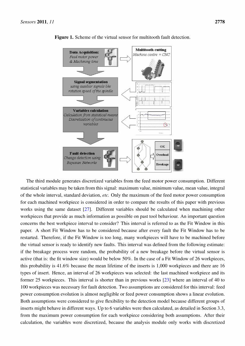
The virtual sensor developed in this work consists of four modules: a data acquisition system capableof extracting information from the cutting process, a segmentation module to identify the informationrelated to each group of cutting inserts, a third module to turn this information into different discretizedvariables and a final module to change the detection of the selected variables based on a Bayesianclassifier for reliable multitooth fault detection. A schematic diagram of the virtual sensor is shownin Figure 1. Thus, Figure 1 also includes images of the crankshafts before and after the machiningoperation on the first body and images of broken and new cutting inserts for the roughing operation.

The first module is composed of the physical sensors that should provide information on the cuttingprocess. There are several kinds of sensors that have been used in the literature for monitoringcutting processes: acoustic emission [35,36], cutting force [37,38], vibration [39,40], electrical powerconsumption [41,42] and noise [43,44]. In our case, a first attempt considered the temperature of themechanized main journals of the crankshafts, vibration, noise and the electrical power of the tool drivesas previously demonstrated in [23]. The electrical power consumption was measured from the outputsignals of the frequency converters of the two main milling machine motors driving the cutting process:the rotation motor and the feed motor showed the best signal-to-noise ratio. As this signal is also the leastinvasive, the cheapest, and remains unaffected by other events that might occur during machining [23],it was considered as the best physical signal for the virtual sensor. Between the two motors in whichconsumption is correlated with tool wear—the rotation motor and the feed motor, the latter showeda clearer correlation with tool faults [23]. The power consumption of the feed motor was thereforeselected as the main input for the virtual sensor.

The second module is responsible for segmentation of the feed motor power consumption. The toolis divided into different groups of inserts, which also correlate with the temporal evolution of electricalpower consumption. Each time a group of inserts engage the workpiece, the milling centre changes thecutting conditions (rotation speed and feedrate). The rotation of the tool is programmed in such a waythat every group of inserts only ever engage each crankshaft once. Therefore, the segmentation of theelectrical power signal for every insert uses tool rotation speed as an auxiliary signal to identify eachgroup of inserts working at any given moment in time.

Sensors 2011, 11 2778

Figure 1. Scheme of the virtual sensor for multitooth fault detection.

The third module generates discretized variables from the feed motor power consumption. Differentstatistical variables may be taken from this signal: maximum value, minimum value, mean value, integralof the whole interval, standard deviation, etc. Only the maximum of the feed motor power consumptionfor each machined workpiece is considered in order to compare the results of this paper with previousworks using the same dataset [27]. Different variables should be calculated when machining otherworkpieces that provide as much information as possible on past tool behaviour. An important questionconcerns the best workpiece interval to consider? This interval is referred to as the Fit Window in thispaper. A short Fit Window has to be considered because after every fault the Fit Window has to berestarted. Therefore, if the Fit Window is too long, many workpieces will have to be machined beforethe virtual sensor is ready to identify new faults. This interval was defined from the following estimate:if the breakage process were random, the probability of a new breakage before the virtual sensor isactive (that is: the fit window size) would be below 50%. In the case of a Fit Window of 26 workpieces,this probability is 41.6% because the mean lifetime of the inserts is 1,000 workpieces and there are 16types of insert. Hence, an interval of 26 workpieces was selected: the last machined workpiece and itsformer 25 workpieces. This interval is shorter than in previous works [23] where an interval of 40 to100 workpieces was necessary for fault detection. Two assumptions are considered for this interval: feedpower consumption evolution is almost negligible or feed power consumption shows a linear evolution.Both assumptions were considered to give flexibility to the detection model because different groups ofinserts might behave in different ways. Up to 6 variables were then calculated, as detailed in Section 3.3,from the maximum power consumption for each workpiece considering both assumptions. After theircalculation, the variables were discretized, because the analysis module only works with discretized

Sensors 2011, 11 2779

variables. For this task, the discretization intervals were selected using data-independent criteria. Thevirtual sensor was therefore able to resolve them by itself for each insert group without the involvementof a human expert.

The last module predicts tool behaviour from the variables that were measured and discretized inthe previous steps. This module uses a Bayesian classifier to select between 3 possible labels for theexpected behaviour of the tool: type: “0” if the tool works properly, “–1” when a overload fault ispresented and “+1” when a insert breakage takes place. The model is capable of detecting online faults inmultitooth tools with probabilities of up to 90% for each fault type. Besides, the main advantage of BNsis their reasoning method, which is based on a model that attempts to convey the physical relationshipsof the process (milling in this case) and other less obvious (perhaps stochastic) relationships between thevariables, not generally analysed in depth in other artificial intelligence-based models. This method incombination with the strong probabilistic theory of the BN generates their particular interpretations. Thepredictive capabilities of the virtual sensor will be explained in detail in Section 4.

3. Experimental Set-Up and Tuning of the Virtual Sensor to a Real Industrial Task

When the general schematic design of the virtual sensor was fully prepared, data from an industrialsetting was collected to set up and to validate the virtual sensor.

3.1. Data Acquisition

Data were gathered from a multitooth tool that mechanizes the five main journals of a crankshaft. Itincludes 200 roughing inserts and around 30 finishing inserts. The tool manufacturer established insertlife spans of around 1,100 workpieces in the case of the roughing inserts. During the machining cycle ofeach crankshaft, cutting conditions were varied according to a predefined profile. This profile relates tothe kind of inserts (dedicated to roughing or finishing) that are spread over the tool’s surface and shouldwork in each cycle instant.

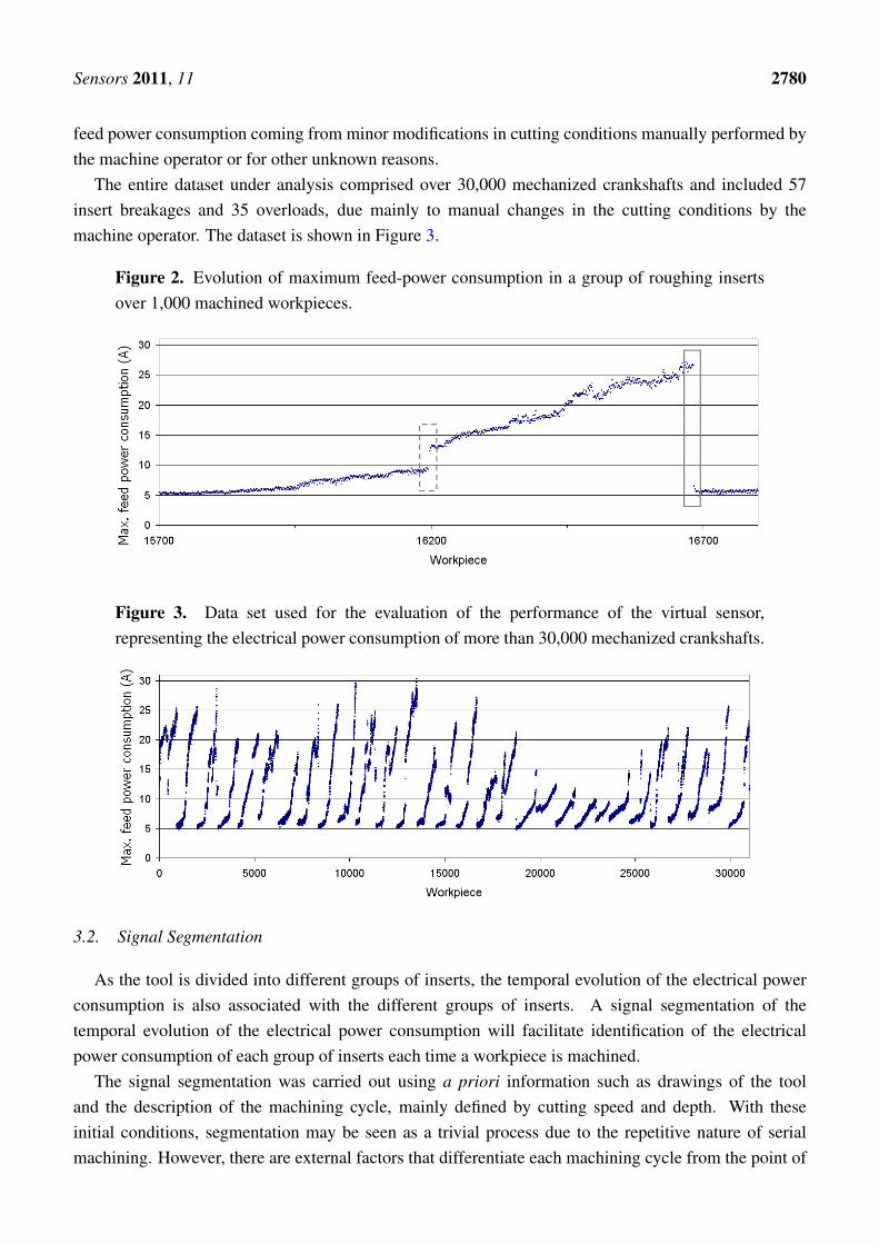
Electrical power consumption is measured from the output signal of the frequency converter in thefeed motor of the milling centre. The equipment used is based on a computer data acquisition system.An industrial PC with a data acquisition board that has a specific data acquisition software programmedin LabVIEW [45] v6.i monitors the different digital signals that handle the machining cycle. Each timea new workpiece starts its machining cycle, the software automatically performs data acquisition andrecording. At the end of the cycle the software computes the diagnostics algorithms to determine whetheranything is going wrong with the multitooth tool, so that the machine tool may if necessary be stopped toperform appropriate maintenance. As already explained, only the maximum of this power consumptionfor each machined workpiece is considered. An analysis of electrical power consumption during thecutting cycle shows how it rises slowly due to tool wear until insert breakage occurs, after which thecorresponding power consumption waveform falls abruptly, as shown in Figure 2. This trend is clearlyobservable in the figure that shows the maximum feed-power consumption of a group of roughing insertsduring the machining of over 1,000 crankshafts. The change instant due to tool breakage is marked by agrey square. This figure also shows overload as a grey dashed square, which signifies a small jump in the

Sensors 2011, 11 2780

feed power consumption coming from minor modifications in cutting conditions manually performed bythe machine operator or for other unknown reasons.

The entire dataset under analysis comprised over 30,000 mechanized crankshafts and included 57insert breakages and 35 overloads, due mainly to manual changes in the cutting conditions by themachine operator. The dataset is shown in Figure 3.

Figure 2. Evolution of maximum feed-power consumption in a group of roughing insertsover 1,000 machined workpieces.

Figure 3. Data set used for the evaluation of the performance of the virtual sensor,representing the electrical power consumption of more than 30,000 mechanized crankshafts.

3.2. Signal Segmentation

As the tool is divided into different groups of inserts, the temporal evolution of the electrical powerconsumption is also associated with the different groups of inserts. A signal segmentation of thetemporal evolution of the electrical power consumption will facilitate identification of the electricalpower consumption of each group of inserts each time a workpiece is machined.

The signal segmentation was carried out using a priori information such as drawings of the tooland the description of the machining cycle, mainly defined by cutting speed and depth. With theseinitial conditions, segmentation may be seen as a trivial process due to the repetitive nature of serialmachining. However, there are external factors that differentiate each machining cycle from the point of

Sensors 2011, 11 2781

view of its temporal evolution. The most important factors that can override the machining cycle are:manufacturing of more than one vehicle component on the same machine line, geometrical uncertaintiesof the component to be machined due to its casting or delays in the component supply line. All thesereasons make it necessary to identify an algorithm that performs robust and reliable signal segmentationfor further processing. A segmentation fault may lead to a false alarm that would affect the reliability ofthe virtual sensor.

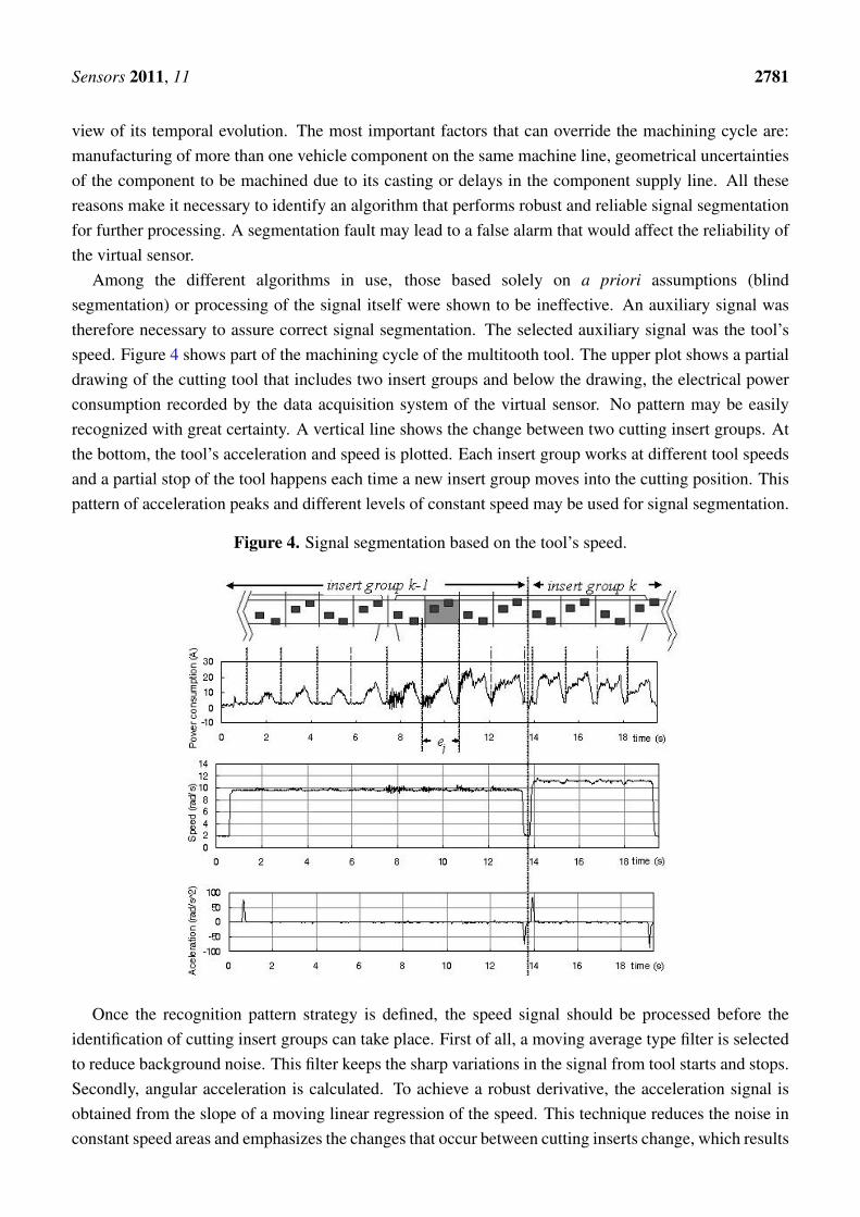
Among the different algorithms in use, those based solely on a priori assumptions (blindsegmentation) or processing of the signal itself were shown to be ineffective. An auxiliary signal wastherefore necessary to assure correct signal segmentation. The selected auxiliary signal was the tool’sspeed. Figure 4 shows part of the machining cycle of the multitooth tool. The upper plot shows a partialdrawing of the cutting tool that includes two insert groups and below the drawing, the electrical powerconsumption recorded by the data acquisition system of the virtual sensor. No pattern may be easilyrecognized with great certainty. A vertical line shows the change between two cutting insert groups. Atthe bottom, the tool’s acceleration and speed is plotted. Each insert group works at different tool speedsand a partial stop of the tool happens each time a new insert group moves into the cutting position. Thispattern of acceleration peaks and different levels of constant speed may be used for signal segmentation.

Figure 4. Signal segmentation based on the tool’s speed.

Once the recognition pattern strategy is defined, the speed signal should be processed before theidentification of cutting insert groups can take place. First of all, a moving average type filter is selectedto reduce background noise. This filter keeps the sharp variations in the signal from tool starts and stops.Secondly, angular acceleration is calculated. To achieve a robust derivative, the acceleration signal isobtained from the slope of a moving linear regression of the speed. This technique reduces the noise inconstant speed areas and emphasizes the changes that occur between cutting inserts change, which results

Sensors 2011, 11 2782

in an auxiliary signal that refers to power consumption segments. Subsequently, the maximum absolutevalue of angular acceleration is then detected by means of a second-order polynomial fit. It is necessaryto avoid the processing of constant speed areas to speed up the detection process of the maximums. Athreshold for angular acceleration was therefore defined, below which the algorithm does not considerthat a maximum could occur. Figure 5 shows an example of the successive stages of processing the tool’sspeed signal.

Figure 5. Processing stages of the tool speed signal.

3.3. Definition and Discretization of Input Variables

The maximum values are extracted from the signal segmentation of the electrical power consumptionby the feed motor for each machined workpiece. From this value, 5 variables (described below) arecalculated considering the behaviour of the tool in the 25 former pieces. Two assumptions may be madefor this interval: either the feed power consumption evolution is almost negligible or the feed powerconsumption already shows a linear evolution. Both assumptions are considered in this work, to ensurethat the virtual sensor is flexible, because different groups of inserts could behave in different ways. Inthe former case, the mean value of the power consumption of the former 25 workpieces is calculated. Inthe latter case, the power consumption linear fit of the former 25 workpieces and its correlation factor arecalculated. Figure 6 shows both fits in one real case. The point under study is workpiece number 16,684,where a breakage occurs. The linear fit of the 25 former pieces predicts a feed power consumption

Sensors 2011, 11 2783

of 19.63 A, and the mean value of the 25 former pieces is 19.74 A. In reality, however, a feed powerconsumption of 13.04 A occurs due to insert breakage. Figure 6 shows the Fit window, the linear fit andits main variables (slope and correlation factor), but also the change between real power consumptionand expected power consumption for both approaches.

Figure 6. Two assumptions of electrical power consumption evolution: constant behaviouror linear evolution.

The following variables are then evaluated:

• Time between last machined workpiece and present workpiece, u1: this is the only variablethat is not obtained from the feed power consumption, which includes information on machinestoppages that could be related to holidays, maintenance programs, manual adjustments made bythe machine operator to cutting parameters, etc. These events can produce changes in the feedpower consumption that are unrelated to tool faults.

• Slope of the linear fit for power consumption evolution, u2: searches for strong slopes in feedpower consumption that usually predict breakage, as already done in Figure 6.

• Correlation factor for last 10 workpieces, u3: evaluates reliability of a linear fit for powerconsumption evolution within a short range of workpieces.

• Correlation factor for last 25 workpieces, u4: evaluates reliability of a linear fit for powerconsumption evolution, as previously shown in Figure 6, within a long range of workpieces.

• Difference between expected power consumption for new workpiece and real value consideringpower consumption linear evolution, u5: searches for strong drops in feed power consumptionconsidering power consumption evolution to be linear.

• Difference between expected power consumption for new workpiece and real value consideringpower consumption constant evolution, u6: searches for strong drops in feed power consumptionconsidering power consumption evolution to be zero.

• Feed power consumption maximum value for the workpiece, u7: searches for very low values thatoccur when tool inserts are either already broken and no longer cut or are completely new.

• Number of machined workpieces since last breakage, u8: this is a further factor that should beconsidered, as tool inserts have a mean lifetime of 1,000 workpieces.

Sensors 2011, 11 2784

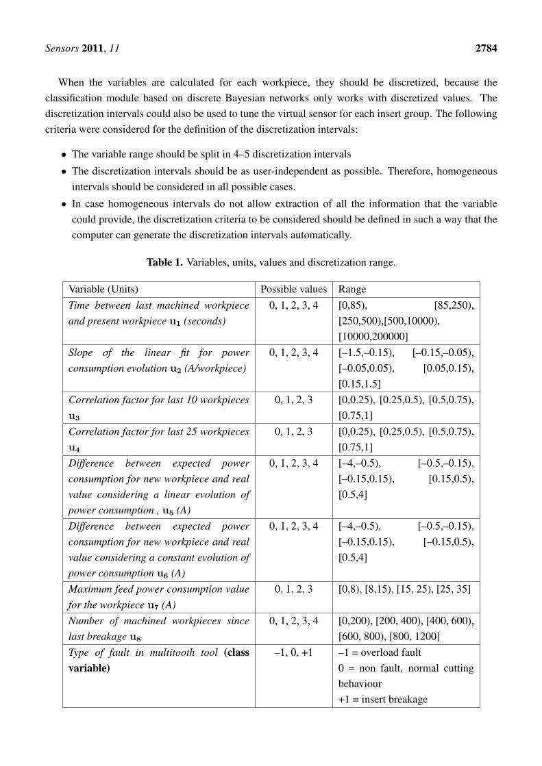
When the variables are calculated for each workpiece, they should be discretized, because theclassification module based on discrete Bayesian networks only works with discretized values. Thediscretization intervals could also be used to tune the virtual sensor for each insert group. The followingcriteria were considered for the definition of the discretization intervals:

• The variable range should be split in 4–5 discretization intervals

• The discretization intervals should be as user-independent as possible. Therefore, homogeneousintervals should be considered in all possible cases.

• In case homogeneous intervals do not allow extraction of all the information that the variablecould provide, the discretization criteria to be considered should be defined in such a way that thecomputer can generate the discretization intervals automatically.

Table 1. Variables, units, values and discretization range.

Variable (Units) Possible values RangeTime between last machined workpieceand present workpiece u1 (seconds)

0, 1, 2, 3, 4 [0,85), [85,250),[250,500),[500,10000),[10000,200000]

Slope of the linear fit for powerconsumption evolution u2 (A/workpiece)

0, 1, 2, 3, 4 [–1.5,–0.15), [–0.15,–0.05),[–0.05,0.05), [0.05,0.15),[0.15,1.5]

Correlation factor for last 10 workpiecesu3

0, 1, 2, 3 [0,0.25), [0.25,0.5), [0.5,0.75),[0.75,1]

Correlation factor for last 25 workpiecesu4

0, 1, 2, 3 [0,0.25), [0.25,0.5), [0.5,0.75),[0.75,1]

Difference between expected powerconsumption for new workpiece and realvalue considering a linear evolution ofpower consumption , u5 (A)

0, 1, 2, 3, 4 [–4,–0.5), [–0.5,–0.15),[–0.15,0.15), [0.15,0.5),[0.5,4]

Difference between expected powerconsumption for new workpiece and realvalue considering a constant evolution ofpower consumption u6 (A)

0, 1, 2, 3, 4 [–4,–0.5), [–0.5,–0.15),[–0.15,0.15), [–0.15,0.5),[0.5,4]

Maximum feed power consumption valuefor the workpiece u7 (A)

0, 1, 2, 3 [0,8), [8,15), [15, 25), [25, 35]

Number of machined workpieces sincelast breakage u8

0, 1, 2, 3, 4 [0,200), [200, 400), [400, 600),[600, 800), [800, 1200]

Type of fault in multitooth tool (classvariable)

–1, 0, +1 –1 = overload fault0 = non fault, normal cuttingbehaviour+1 = insert breakage

Sensors 2011, 11 2785

Table 1 summarises the considered variables and shows the discretization intervals considered foreach variable. It can be seen that all variables are discretized at less than 5 levels. Some of the variables,such as u3, u4 and u8 are discretized in homogeneous intervals. Other variables that have a variationrange symmetric around 0, such as u2, u5 and u6, were discretized in symmetric intervals of around 0with shorter intervals close to this point to increase the sensibility of the virtual sensor. The third groupis composed of two variables: u1 and u7, which often show a value of 250 and 15, respectively. Theintervals are defined in such a way that two homogeneous intervals cover the range from the minimumvalue of the variable up to the most frequently occurring value, and three homogeneous intervals coverthe range from this value to the maximum value. Thus, discretization may be automatically completedby the virtual sensor for each insert group and can clearly separate the behavior associated with the mostfrequently occurring value.

3.4. Bayesian Classifier

A dataset of 9 columns and 377 rows was formed to build a multitooth tool fault detection modelfor the virtual sensor. Each column of the dataset is a variable (the last is the class or network output)and each row is a machined workpiece. From the 377 machined workpieces, 285 showed no faults, 57presented insert breakages and 35 overloads.

Before building the network of the Bayesian classifier a feature subset selection was performed todiscard irrelevant variables. The goodness of a subset of variables was assessed by using a filter approach,i.e., ranking the variables in terms of some scoring metric usually based on intrinsic characteristics of thedata computed from simple statistics on their empirical distribution. Here, information gain is selectedwith regard to class variables as the scoring metric to evaluate the value of a variable. Information gainI(class,X) is the difference between the entropy of class and the conditional entropy of class givenX for any variable X . Weka [46] software, a free suite of machine learning software written in Java,developed at the University of Waikato (New Zealand), was used for this network learning process.Different structures were tested to build the BN structure that achieves the highest breakage detectionrate. The best structure was identified when only 5 variables were selected: u5, u6, u7, u1 and u8. Theaccuracy of this network was 98% compared, for example, with the figure of 97% for the network thatincorporates all 8 variables.

Figure 7 shows the TAN structure built with the 5 selected variables. It illustrates the relationshipsexisting between its nodes, which provide further information on the relationship of each variable withthe class and on the relationship between all the predictor variables. The TAN network that is built alsoinvolves estimating all the conditional probability distributions of each variable given its parents, that isto say, its quantitative part. Given certain evidence (i.e., observations), we can reason in any directionfrom any BN, querying the network about any marginal probability or any posterior probability .

Analyzing the network structure shows that the two variables u5 and u6 have the greatest influence onthe fault type detected by the model. This relation was expected, as these variables collect informationon sudden changes of power consumption when a breakage or an overload occurs while machining apiece. These are therefore the variables that best detect and identify the fault type during the machiningprocess: the class or output variable.

Sensors 2011, 11 2786

Figure 7. Bayesian network TAN structure.

Variable u7 measures power consumption for the workpiece. This value is very high in overloads andvery low when a breakage occurs, so it also has an important relationship with the fault type.

On the other hand, the influence of variables u1 and u8 and their relation to power consumption u7

may also be appreciated. In u1, information is provided on machine time between workpieces; a variablethat reflects stoppages on the production line, maintenance adjustments, etc., which especially influencesoverloads faults, which are not reflected in other variables. In u8, the number of machined parts beforetool breakages is recorded, which is also related to the state of the tool and the fault type that is detected.

The next section details an analysis of the results obtained with the Bayesian classifier for faultdetection in multitooth tools.

4. Results and Discussion

As is well known, the models should not be validated with the same data used for training, for whichpurpose the 10-fold cross-validation [47] method was used. The initial dataset is divided into 10 subsets,of which only one subset is retained as the validation data for testing the model, and the other 9 subsetsare used as training data. The cross-validation process is repeated 10 times (the folds), with each of the10 subsamples used exactly once as the validation data. Then, the 10 results from the folds are averaged(or otherwise combined) to produce a single estimate of the accuracy of the classifier.

The accuracy of a model that is constructed in this way is high (98%), where accuracy is defined asthe number of correct predictions over the number of samples. Accuracy is the most commonly usedmetric to evaluate the performance of a classifier, i.e., an indicator of how good a classifier is or theprobability of it classifying new cases correctly. But accuracy is not sufficient to determine the bestmodel in this industrial process, because in this case the identification of tool breakage is more importantthan normal cutting behaviour. To clarify this point, consider a classifier that correctly identifies all theNon Fault cases but all Breakages cases are wrongly classified as overloads; this classifier will showa high accuracy, because there are very many more Non Fault cases than Breakages in the dataset, but

Sensors 2011, 11 2787

the virtual sensor will be unable to identify the critical cases (tool breakage), which means that it wouldtherefore be useless for industrial purposes. Other measures should also be defined and evaluated toassure correct classifier performance. To build these measures, a confusion matrix should be constructedthat considers how many cases of each class Ci (real) have been classified in each class Ci (assigned),see Table 2. The following measures may then be considered: True Positive Rate (Sensitivity), TrueNegative Rate (Specificity), False Positive Rate and Precision.

Table 2. Confusion matrix for more than 2 classes.

(category i)Assigned →Real ↓

C1 C2 . . . Ci

C1 N11 N12 . . . N1i

C2 N21 N22 . . . N2i

. . . . . . . . . . . .Ci Ni1 Ni2 . . . Nii

Sensitivity or TPR (True Positive Rate) represents the proportion of items classified as belonging toclass Ci, from among everything that really belongs to class Ci. In the confusion matrix (Table 2), it isthe diagonal item divided by the sum of all elements of the row (Equation 2). When relevant sensitivitiesfor each instance of class tends towards 1, the confusion matrix will tend to be a diagonal matrix.

TP Rate (for 2 values) =TP

(TP + FN)(2)

TP Rate(C1) =N11

N11 +N12 + . . .+N1i

...

TP Rate(Ci) =Nii

Ni1 +Ni2 + . . .+Nii

False Positive Rate is the proportion of items that have been classified into class Ci, but belong to adifferent class. In the confusion matrix, it is the sum of the column Ci class minus the diagonal item,divided by the sum of the rows of all other classes (Equation 3).

FP Rate (for 2 values) =FP

(FP + TN)(3)

FP Rate(C1) =N11 +N11 + . . .+Ni1 −N11

[(N21 + . . .+N2i) + (N31 + . . .+N3i) + . . .+ (Ni1 + . . .+Nii)]...

FP Rate(Ci) =N1i +N2i + . . .+Nii −Nii

[(N11 + . . .+N1i) + (N21 + . . .+N2i) + . . .+ (N(i−1)1 + . . .+N(i−1)i)]

Sensors 2011, 11 2788

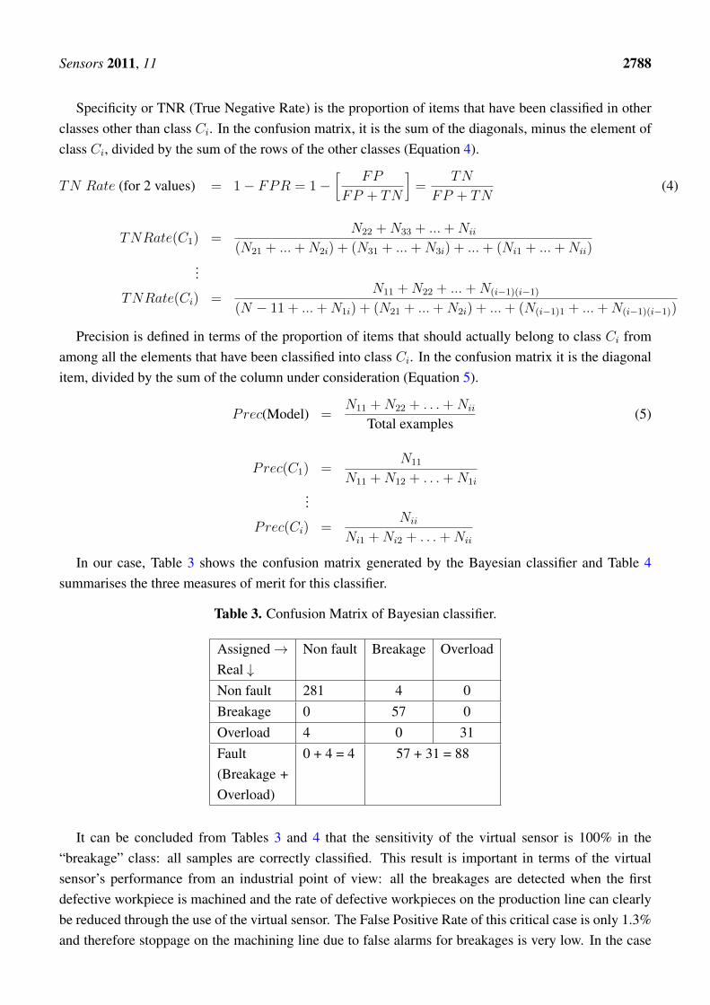
Specificity or TNR (True Negative Rate) is the proportion of items that have been classified in otherclasses other than class Ci. In the confusion matrix, it is the sum of the diagonals, minus the element ofclass Ci, divided by the sum of the rows of the other classes (Equation 4).

TN Rate (for 2 values) = 1− FPR = 1−[

FP

FP + TN

]=

TN

FP + TN(4)

TNRate(C1) =N22 +N33 + ...+Nii

(N21 + ...+N2i) + (N31 + ...+N3i) + ...+ (Ni1 + ...+Nii)...

TNRate(Ci) =N11 +N22 + ...+N(i−1)(i−1)

(N − 11 + ...+N1i) + (N21 + ...+N2i) + ...+ (N(i−1)1 + ...+N(i−1)(i−1))

Precision is defined in terms of the proportion of items that should actually belong to class Ci fromamong all the elements that have been classified into class Ci. In the confusion matrix it is the diagonalitem, divided by the sum of the column under consideration (Equation 5).

Prec(Model) =N11 +N22 + . . .+Nii

Total examples(5)

Prec(C1) =N11

N11 +N12 + . . .+N1i

...

Prec(Ci) =Nii

Ni1 +Ni2 + . . .+Nii

In our case, Table 3 shows the confusion matrix generated by the Bayesian classifier and Table 4summarises the three measures of merit for this classifier.

Table 3. Confusion Matrix of Bayesian classifier.

Assigned →Real ↓

Non fault Breakage Overload

Non fault 281 4 0Breakage 0 57 0Overload 4 0 31Fault(Breakage +Overload)

0 + 4 = 4 57 + 31 = 88

It can be concluded from Tables 3 and 4 that the sensitivity of the virtual sensor is 100% in the“breakage” class: all samples are correctly classified. This result is important in terms of the virtualsensor’s performance from an industrial point of view: all the breakages are detected when the firstdefective workpiece is machined and the rate of defective workpieces on the production line can clearlybe reduced through the use of the virtual sensor. The False Positive Rate of this critical case is only 1.3%and therefore stoppage on the machining line due to false alarms for breakages is very low. In the case

Sensors 2011, 11 2789

of overloads, the classification accuracy is lower, at 88.6%. This result is expected, because the overloadclass occurs less often in the dataset. This lower rate of overload detection does not matter from anindustrial point of view, because overloads are not critical for tool performance or workpiece machiningand the virtual sensor will only generate an alarm to notify the operator that something unexpected butnot critical has occurred.

Table 4. Accuracy by class of Bayesian classifier.

Class TP Rate FP Rate PrecisionNon fault 0.986 0.043 0.986Breakage 1 0.013 0.934Overload 0.886 0 1Fault 0.957 0.014 0.957

Comparison of the BN classifier with a former work on the same dataset [23] joins fault types,overloads and breakages in one category called “Fault” in Tables 3 and 4, the last row of which showsthe classifier’s performance in the Fault class. In this case, the classification accuracy of the modelis 96.4%. Other algorithms used to solve this industrial problem in a former work were the LRODalgorithm, CUSUM and time series forecasting [23]. LROD showed the best capabilities to solve thisproblem. Therefore a comparison between LROD and the new virtual sensor was conducted. The LRODalgorithm has three parameters to be fixed: the window size L, the fault’s threshold h and the run testparameter R. Different fits were tested [23] and their performance was compared with that of the newvirtual sensor. The results are shown in Table 5. The objective searched for each LROD fit, which are alsoshown in this table. Performance is evaluated in terms of 4 criteria: MTFA, MTD, Fault classificationaccuracy and Fit Window.

Table 5. Comparison of the performance of LROD algorithm and classifier ensembles forimbalanced datasets.

Linear Regression Outlier Detection NewParameters R = 2, h = 4 R = 3, h = 2.5 R = 2, h = 1.1 R = 4, h = 3.5 Virtual

Minimum Trade-off Maximum Shorter SensorCriteria MTD point %Detected Fit Window

MTFA 2000 400 50 1000 463

MTD 2 6 4.5 3.5 1

%Detected 85% 93% 98% 88% 96.4%

Fit Window 70 70 70 40 25

It can be concluded that the LROD algorithm required a Fit Window of approximately 70 workpiecesto achieve a percentage fault detection rate higher than 90%, while the virtual sensor required a FitWindow of only 26 workpieces to achieve a rate of 96.4%. If a shorter Fit Window is selected, forexample 40 workpieces, the percentage of detected breakages for LROD drops to 88% in the bestcase. When a higher accuracy than 90% was sought, the LROD fit presented a MTD of more than

Sensors 2011, 11 2790

4.5 workpieces and a MTFA lower than 400 workpieces, which makes it an expensive solution becauseit would lead to many false alarms and unnecessary stoppages, and many defective workpieces would bemachined. If MTD is decreased, LROD also looses precision and for a 2 workpiece MTD, only 85% ofbreakages can be detected. The virtual sensor presents an MTD of only 1 workpiece. The MTFA of thevirtual sensor is not as good as some of the LROD fits, but its better performance in terms of accuracyand Fit Window with respect to these fits makes it the better solution. It should be noted that accuracyin this comparison was considered for the Fault class because former works do not split their resultsbetween Breakage and Overload classes, but the really critical class from the industrial point of view-Breakages- shows a true positive rate of 100% with the new virtual sensor.

In addition to its better overall performance, the new virtual sensor based on the Bayesian modelpresents a further advantage over the LROD algorithm: its reasoning capability. Given certain evidence,the BN may be queried on issues including observations or evidence, in order to find the posteriorprobability of any variable or set of variables. This can produce different types of reasoning.

One type of question is predictive reasoning or causal inference. For example, the question maybe asked: what is the probability of each class (fault type) given certain manufacturing requirements?The response is a prediction of effects. If a batch of workpieces of between [800, 1,200] units witha maximum feed power consumption value has to be produced, the BN may be asked to computeP (class|u8 = 4, u7 = 3). Propagating this evidence, the network will compute the following classprobabilities: non-fault with a probability of 0.46, Insert breakage with a probability of 0.33 andOverload fault with a probability of 0.21. Given these requirements, the highest probabilities are fornon faults; which fits with the experimental dataset.

Questions relating to diagnostic reasoning may also be asked, such as “what are the probabilities ofunobserved variables if class is restricted?” Let us suppose that we need to detect when a failure toolbreakage will cause (class = Insert breakage) at the time of manufacturing a batch of workpieces (u8)between [400, 600), and that we need to establish the recommendations of the model with regard tomaximum feed power consumption (u7) and machine time between workpieces (u1), so as to detect thattype of tool breakage; in which case P (u7, u1|class = insert breakage, u8 = [400, 600)) is calculated.Moreover, a further advantage of BNs is the possibility of finding the most likely explanation or abductiveinference. In this case, we look for the configurations of these two variables with the highest probability.The network informs us that the probability that this type of fault will occur increases as both machinetime between workpieces and the maximum feed power consumption increase.

A total abduction finds the configuration of all the unobserved variables that maximize the evidenceprobability, e.g., argmaxx1,...,xn P (x1, . . . , xn|class = insert breakage). In this case, the most likelyconfiguration is u5 at [–4, –0.5), u6 at [–4, –0.5), u7 at [0, 8), u1 at 3 [800, 1,200] and u8 at4 [500, 10,000]. Thus, the most likely configuration of the remaining five variables responds to thequestion that concerns the conditions which have a higher probability of causing an insert breakagefault.

Another way to understand the usefulness of this capability of the virtual sensor is, for example, toschedule preventive tool changes. In this case, RB introduced evidence in two variables: (i) number ofmachined workpieces u8 and (ii) feed power consumption maximum u7. The assumptions are normalmachining with low feed power consumption (u7 = 0) for the manufacture of 350 pieces (u8 = 1),

Sensors 2011, 11 2791

where the probability of breakage insert and overload fault is very low (0.062 and 0.038 respectively).The probability of insert breakages when the number of workpieces are increased may be calculatedas follows: P (class|u7 = 0, u8 = 2). In this case, the probability of insert breakage and faultsincreases slightly without undue cause for alarm (0.128 and 0.079 respectively). However, the increasedprobability is considerable when P (class|u7 = 0, u8 = 3) is calculated: breakage 0.407 and faults0.251, in the case of P (class|u7 = 0, u8 = 4) there is an increased probability of breakage at 0.56 and afault probability at 0.346. From these results, we see that it is essential to change the tool when over 800units produced.

5. Conclusions and Futures Lines of Work

This paper has presented a new virtual sensor for multitooth tool fault detection in the automotiveindustry. The proposed virtual sensor is based on electrical power consumption analysis and a Bayesiannetwork. The application to a real case, the final machining of vehicle crankshafts on a mass productionline was also presented and compared with a parallel methodology using the Linear Regression OutlierDetection Algorithm. The virtual sensor is defined as an alternative to the allocation of a suitablesensors close to the tool tip on the milling centres, because this strategy is not possible in industrialenvironments. The virtual sensor definition has to be capable of solving the problems that may occurwith multitooth tools, especially complex machining tools with different kinds of inserts that performdifferent consecutive cutting operations on the same workpiece.

The virtual sensor consists of four modules: a data acquisition system capable of extractinginformation from the cutting process, a segmentation module to identify the information related to eachkind of cutting inserts, a third module to turn this information in different discretized variables and afinal module to change detection of the selected variables based on Bayesian classifiers in a way that isreliable for multitooth fault detection.

The virtual sensor detects faults through changes in electrical power consumption. As the tool isdivided into different groups of inserts, the temporal evolution of the electrical power consumption isalso associated with the different groups of inserts. The rotation speed of the machine spindle is usedto identify the right time window for each insert group because the programmed rotation speed for eachinsert group is different.

As the electrical power consumption undergoes an abrupt change when a tool fault occurs, theproblem of fault detection in a multitooth tool could be reformulated as a detection problem that usesdifferent statistical variables of the electrical power consumption associated with the different groups oftool inserts, most of which consider the behaviour of the same tool during the machining of the former 25workpieces. When the variables are calculated for each workpiece, they should be discretized becausethe Bayesian networks module only works with discretized values. The discretization intervals couldalso be used to tune the virtual sensor for each insert group. The discretization intervals were calculatedusing data-independent criteria. Therefore the virtual sensor could fix them by itself for each insert groupwithout the interaction of a human expert.

The effective communication of an alarm after cutting operations on a workpiece must be made ina reliable manner, applying consistency checks and auxiliary information (cutting parameter changes,planned maintenance operations, etc.) for the process. This paper is mainly devoted to change detection

Sensors 2011, 11 2792

and decision-making using a Bayesian model; an alternative that has mainly been chosen because ofits potential to track and explain the process, which was tuned with the aid of different performancemeasurements. The interpretation capabilities of Bayesian networks allow the use of the virtual sensornot only as a fault detection sensor, but also as a predictive tool for machine line maintenance.

The new virtual sensor overcomes important drawbacks of the former proposed methodology basedon the Linear Regression Outlier Detection Algorithm. The first is that the virtual sensor tuning iscompletely automated and does not depend on prior user knowledge of the cutting process. Thus, ifa new multitooth tool is installed or the cutting process is changed, the auto-tuning capability of thevirtual sensor can respond to this situation. The second it is that only a 26 workpiece interval beforethe workpiece that is machined in real time is necessary for fault detection. In previous works, a 40–70workpiece interval was considered necessary to achieve high reliability. The new virtual sensor wastherefore able to detect faults within a shorter period after the last fault. The third advantage is thatthe interval needed for fault detection with a high degree of reliability (higher than 95%) is reducedfrom the 4 workpieces cited in earlier works to 1 workpiece, which in turn drastically reduces defectiveworkpieces produced on the machine line.

Future work will focus on the application of the virtual sensor to other kinds of industrial problemson which fault detection searches are conducted and a continuous degradation of certain variablesis expected before fault detection occurs. Examples could be drill breakage during the drilling ofmultilayer sheets for the manufacture of aeronautical components, or mill breakages during the millingof aluminium ribs for aeroplanes.

Acknowledgements

This work has been made possible thanks to the support received from the Red de Supervisiony Diagnosis de Sistemas Complejos (DPI2009-06124-E) of the Spanish Ministry of Science andInnovation.

References and Notes

1. Du, R.; Elbestawi, M.A.; Wu, S.M. Automated monitoring of manufacturing processes. Part 1:Monitoring methods. J. Eng. Indust. 1995, 117, 121–132.

2. Altintas, Y. Manufacturing Automation: Metal Cutting Mechanics, Machine Tool Vibrations andCNC Design; Cambridge University Press: New York, NY, USA, 2000.

3. Astakhov, V.P. The assessment of cutting tool wear. Int. J. Mach. Tool. Manufact. 2004,44, 637–647.

4. Liang, S.Y.; Hecker, R.L.; Landers, R.G. Machining process monitoring and control: The state ofthe art. J. Manufact. Sci. Eng. 2004, 126, 297–310.

5. Frankowiak, M.; Grosvenor, R.; Prickett, P. A review of the evolution of microcontroller-basedmachine and process monitoring. Int. J. Mach. Tool. Manufact. 2005, 45, 573–582.

6. Caroprese, L.; Comito, C.; Talia, D.; Zumpano, E. A logic approach to virtual sensor networks. InProceedings of IDEAS ’10: The Fourteenth International Database Engineering and ApplicationsSymposium, Montreal, QC, Canada, 16–18 August 2010; pp. 149–156.

Sensors 2011, 11 2793

7. Kabadayi, S.; Pridgen, A.; Julien, C. Virtual sensors: Abstracting data from physical sensors.In Proceedings of WoWMoM’06: International Symposium on a World of Wireless, Mobile andMultimedia Networks, Buffalo, NY, USA, 26–29 June 2006; pp. 586–592.

8. Heredia, G.; Ollero, A. Virtual sensor for failure detection, identification and recovery in thetransition phase of a morphing aircraft. Sensors 2010, 10, 2188–2201.

9. Rallo, R.; Ferre-Gine, J.; Arenas, A.; Giralt, F. Neural virtual sensor for the inferential predictionof product quality from process variables. Comput. Chem. Eng. 2002, 26, 1735-1754.

10. Ibarguengoytia, P.; Delgadillo, M. On-line viscosity virtual sensor for optimizing the combustionin power plants. In Proceedings of IBERAMIA 2010: Advances in Artificial Intelligence, BahıaBlanca, Argentina, 1–5 November 2010; pp. 463–472.

11. Jemielniak, K. Commercial tool condition monitoring systems. Int. J. Adv. Manufact. Techn.1999, 15, 711–721.

12. Romero-Troncoso, R.D.J.; Herrera-Ruiz, G.; Terol-Villalobos, I.; Jauregui-Correa, J.C. Drivercurrent analysis for sensorless tool breakage monitoring of CNC milling machines. Int. J. Mach.Tool. Manufact. 2003, 43, 1529–1534.

13. Altintas, Y.; Shamoto, E.; Lee, P.; Budak, E. Analytical prediction of stability lobes in ball endmilling. J. Manufact. Sci. Eng. 1999, 121, 586–592.

14. Abu-Mahfouz, I. Drilling wear detection and classification using vibration signals and artificialneural network. Int. J. Mach. Tool. Manufact. 2003, 43, 707–720.

15. Kamarthi, S.V.; Kumara, S.R.T.; Cohen, P.H. Flank wear estimation in turning through waveletrepresentation of acoustic emission signals. J. Manufact. Sci. Eng. 2000, 122, 12–19.

16. Wu, Y.; Escande, P.; Du, R. A new method for real-time tool condition monitoring in transfermachining stations. J. Manufact. Sci. Eng. 2001, 123, 339–347.

17. Du, R.; Elbestawi, M.A.; Wu, S.M. Automated monitoring of manufacturing processes. Part 2:Applications. J. Eng. Indust. 1995, 117, 133–141.

18. Li, X.; Patri, K.V.; Cheng, M.K. Feed cutting force estimation from the current measurement withhybrid learning. Int. J. Adv. Manufact. Techn. 2000, 16, 859–862.

19. Haber, R.E.; Alique, J.R.; Alique, A.; Hernandez, J.; Uribe-Etxebarria, R. Embedded fuzzy-controlsystem for machining processes: Results of a case study. Comput. Indust. 2003, 50, 353–366.

20. Scheffer, C.; Kratz, H.; Heyns, P.S.; Klocke, F. Development of a tool wear-monitoring system forhard turning. Int. J. Mach. Tool. Manufact. 2003, 43, 973-985.

21. Zahra, N.H.; Yu, G. Gradual wear monitoring of turning inserts using wavelet analysis ofultrasound waves. Int. J. Mach. Tool. Manufact. 2003, 43, 337–343.

22. Portillo, E.; Marcos, M.; Cabanes, I.; Zubizarreta, A. Recurrent ANN for monitoring degradedbehaviours in a range of workpiece thicknesses. Eng. Appl. Artif. Intell. 2009, 22, 1270 – 1283.

23. Renones, A.; de Miguel, L.J.; Peran, J.R. Experimental analysis of change detection algorithmsfor multitooth machine tool fault detection. Mech. Syst. Sign. Process. 2009, 23, 2320–2335.

24. Rivero, A.; de Lacalle, L.L.; Penalva, M.L. Tool wear detection in dry high-speed milling basedupon the analysis of machine internal signals. Mechatronics 2008, 18, 627–633.

Sensors 2011, 11 2794

25. Loenzo, R.A.G.; Lumbreras, P.D.A.; de Jesus Romero Troncoso, R.; Ruiz, G.H. An object-orientedarchitecture for sensorless cutting force feedback for CNC milling process monitoring and control.Adv. Eng. Softw. 2010, 41, 754–761.

26. Shinno, H.; Hashizume, H.; Yoshloka, H. Sensor-less monitoring of cutting force duringultraprecision machining. CIRP Ann. Manufact. Techn. 2003, 52, 303–306.

27. Renones, A.; Rodriguez, J.; de Miguel, L. Industrial application of a multitooth tool breakagedetection system using spindle motor electrical power consumption. Int. J. Adv. Manufact. Techn.2010, 46, 517–528.

28. Minsky, M. Steps toward artificial intelligence. Trans. Instit. Radio Eng. 1961, 49, 8-30.29. Friedman, N.; Geiger, D.; Goldszmidt, M. Bayesian network classifiers. Mach. Learn. 1997,

29, 131–163.30. Chow, C.; Liu, C. Approximating discrete probability distributions with dependence trees. IEEE

Trans. Inform. Theory 1968, 14, 462–467.31. Mechraoui, A.; Medjaher, K.; Zerhouni, N. Bayesian based fault diagnosis: Application to an

electrical motor. In Proceedings of 17th Triennal World Congress of the International Federationof Automatic Control, Seoul, Korea, 6–11 July 2008; pp. 7381–7386.

32. Oukhellou, L.; Come, E.; Bouillaut, L.; Aknin, P. Combined use of sensor data and structuralknowledge processed by Bayesian network: Application to a railway diagnosis aid scheme.Transport. Rese. Part C: Emerg. Techn. 2008, 16, 755–767.

33. Ramırez, J.C.; Munoz, G.; Gutierrez, L. Fault Diagnosis in an Industrial Process UsingBayesian Networks: Application of the Junction Tree Algorithm. In Proceedings of CERMA2009: Electronics, Robotics and Automotive Mechanics Conference, Cuernavaca, Mexico, 22–25September 2009; pp. 301–306.

34. Basseville, M.; Nikiforov, I. Detection of Abrupt Changes: Theory and Application; PTR PrenticeHall: Englewood Cliffs, NJ, USA, 1993.

35. Kamarthi, S.; Kumara, S.; Cohen, P. Flank wear estimation in turning through waveletrepresentation of acoustic emission signals. J. Manufact. Sci. Eng. 2000, 122, 12–19.

36. Mesina, O.; Langari, R. A neuro-fuzzy system for tool condition monitoring in metal cutting.J. Manufact. Sci. Eng. 2001, 123, 312–318.

37. Scheffer, C.; Kratz, H.; Heyns, P.; Klocke, F. Development of a tool wear-monitoring system forhard turning. Int. J. Mach. Tool. Manufact. 2003, 43, 973–985.

38. Altintas, Y. Manufacturing Automation: Metal Cutting Mechanics, Machine Tool Vibrations, andCNC Design; Cambridge University Press: New York, NY, USA, 2000.

39. Tlusty, J. Manufacturing Processes and Equipment; PTR Prentice Hall: Englewood Cliffs, NJ,USA, 2000.

40. Trejo Hernandez, M.; Osornio Rios, R.A.; Romero Troncoso, R.D.J.; Rodriguez Donate, C.;Dominguez Gonzalez, A.; Herrera Ruiz, G. FPGA-based fused smart-sensor for tool-wear areaquantitative estimation in CNC machine inserts. Sensors 2010, 10, 3373–3388.

41. Altintas, Y. Prediction of cutting forces and tool breakage in milling from feed drive currentmeasurements. J. Eng. Indust. 1992, 114, 386–392.

Sensors 2011, 11 2795

42. Stein, J.; Huh, K. Monitoring cutting forces in turning: A model-based approach. J. Manufact.Sci. Eng. 2002, 124, 26–31.

43. Rahman, M. In-process detection of chatter threshold. J. Eng. Indust. 1988, 110, 44–50.44. Altintas, Y.; Shamoto, E.; Lee, P.; Budak, E. Analytical prediction of stability lobes in ball end

milling. J. Manufact. Sci. Eng. 1999, 121, 586–592.45. National Instruments, Austin, TX, USA. Available online: http://www.ni.com/labview/ (accessed

on 12 February 2011).46. The WEKA Data Mining Software. Available online: http://www.cs.waikato.ac.nz/ml/weka/

(accessed on 12 February 2011).47. Stone, M. Cross-validatory choice and assessment of statistical predictions. J. Roy. Statist. Soc. B

1974, 36, 211–147.

c⃝ 2011 by the authors; licensee MDPI, Basel, Switzerland. This article is an open access articledistributed under the terms and conditions of the Creative Commons Attribution license(http://creativecommons.org/licenses/by/3.0/.)