Probabilistic Model for Sensor Fault Detectionand IdentificationNasir Mehranbod and Masoud Soroush

Dept. of Chemical Engineering, Drexel University, Philadelphia, PA 19104

Michael PiovosoPennsylvania State University, School of Graduate Professional Studies, Malvern, PA 19355

Babatunde A. OgunnaikeDuPont Central Science and Engineering, Experimental Station, E1r104,Wilmington, DE 19880

( )A new Bayesian belief network BBN model with discretized nodes is proposed forfault detection and identification in a single sensor. The single-sensor model is used as abuilding block to de®elop a BBN model for all sensors in the process considered. A newfault detection index, a fault identification index, and a threshold setting procedure forthe multisensor model are introduced. The fault detection index exploits the probabilisticinformation of the multisensor model, which, along with the proposed threshold settingprocedure, leads to effecti®e detection of faulty sensors. The fault identification indexuses only the probabilistic information of the faulty sensor to determine in a discretizedfashion the size of faults that should be analyzed within a mo®ing time window to

(identify the fault type. Single-sensor model design parameters prior and conditional)probability data are optimized to achie®e maximum effecti®eness in detection and iden-

tification of sensor faults. The single-sensor model and optimal ®alues of design param-eters are used to de®elop a multisensor BBN model for a polymerization reactor atsteady-state conditions. Its capabilities to detect and identify bias, drift, and noise insensor readings are illustrated for single and simultaneous multiple faults by se®eral casestudies.

Introduction

To achieve effective controlrmonitoring of a process, re-gardless of its complexity, reliable measurements from the

Ž .process sensors are needed. An instrument sensor oftencomprises of different parts such as a sensing device, trans-ducer, signal processor, and communication interface. Any ofthese parts may malfunction causing the sensor to generatesignals with unacceptable deviation from its normal condi-

Ž .tion. A sensor working under this condition faulty sensormay cause process performance degradation, process shut-down, or even fatal accidents. To determine the presence of

Žfaulty sensors in a process and the type of the faults bias,

Correspondence concerning this article should be addressed to M. Soroush.

.drift, noise, or complete failure , a method of instrument faultŽ .detection and identification IFDI is needed. Processes like

nuclear power plants and highly exothermic chemical reac-tors are safety-critical in nature, and IFDI is of vital impor-tance to their safe and effective operation. The application ofIFDI is not restricted to extreme cases such as nuclear powerplants, and the benefits of IFDI implementation are well rec-

Ž .ognized in other fields Lee et al., 1997 . Because of strictersafety and environmental regulations, as well as increasinglycompetitive global market conditions, IFDI has in recentyears received more attention.

Preventive maintenance and automated techniques arecommon methods of IFDI. Preventive maintenance is basi-

July 2003 Vol. 49, No. 7AIChE Journal 1787

cally regular checking and calibration of sensors. Even thetedious procedure of preventive maintenance cannot guaran-tee a sensor fault-free system, and, hence, it cannot be con-sidered as a perfect alternative for an automated and effi-cient IFDI system. The automated IFDI techniques that arebased on either analytical or physical redundancy methodsŽ . Ž .Betta and Pietrosanto, 2000 . Measuring inferring a param-

Ž .eterrvariable by from more than one sensor is the basis ofŽthe physical redundancy methods Park and Lee, 1993; Alag

.et al., 1995; Dorr et al., 1997 . For the purpose of fault detec-tion, only two measurements are enough. However, to extendthis to fault isolation, three or more measurements are neces-sary. The physical redundancy methods are relatively easy toimplement. They provide a high degree of certainty, althoughthey suffer from the disadvantage of requiring additional sen-sors.

Kalman filters, Luenberger observers, parity relations,Ž .principal component analysis PCA , and artificial neural net-

works are the analytical redundancy methods that have re-ceived a lot of attention. Kalman filters and Luenberger ob-

Žservers have been used widely for IFDI Clark et al., 1975;Clark, 1978a,b; Frank and Keller, 1980; Patton and Chen,

.1997 . Apart from the inadequacies that may be caused bythe linear approximation of process model used in EKF, one

Ž .needs a set of ‘‘matched filters’’ dedicated observers for eachŽsensor to perform fault isolation task Mehra and Peshon,

1971; Watanabe and Himmelblau, 1982; Watanabe et al.,.1994 . The application of Kalman filters and Luenberger ob-

servers requires a process model. However, the existence ofsystematic methods of designing filters and observers is a ma-jor advantage.

ŽPCA and parity relations are closely related Gertler and.McAvoy, 1997 and are applied for fault detection and diag-

Ž .nosis Gertler and McAvoy, 1997; Gertler et al., 1999 . PCAhas proved to be an effective tool for monitoring of complex

Žchemical processes MacGregor, 1989; Kresta et al., 1991; Pi-.ovoso et al., 1992a,b; Wise et al., 1995 and has been success-

fully used for IFDI for processes operated at steady stateŽ .Qin and Li, 1999 . The main feature of PCA, its capability ofreducing the dimensionality of the process model, has made

Žit an attractive and currently active research field Valle et.al., 2000; Yoon and MacGregor, 2000 . Artificial neural net-

Žworks have been used for gross error detection Sanchez etal., 1996; Aldrich and Van Deventer, 1994; Terry and Him-

.melblau, 1993; Gupta and Shankar, 1993; Kramer, 1992 andin combination with a state observer as an isolation tool for

Ž .faulty sensors Bulsari et al., 1991 .There have been a few attempts to apply Bayesian belief

networks for fault detection and diagnosis. Kirch andŽ .Kroschel 1994 proposed an approach to present a BBN

model in the form of a set of nonlinear equations and con-straints that should be solved for the unknown probabilities.

Ž .As an inference tool, Rojas-Guzman and Kramer 1993 usedthe genetic algorithm in BBN for fault diagnosis. Santoso et

Ž .al. 1999 exploited the learning capability of Bayesian beliefnetworks to use process data in an adaptable fault diagnosisstrategy. Bayesian belief networks have also been applied for

Ž .IFDI. While Nicholson and Brady 1992 and IbarguengoytiaŽ .et al. 1996 focused on detection of faulty sensors, Aradhye

Ž .1997 explored the use of Bayesian belief networks for bothdetection and identification of sensor faults. However, he

considered an ideal case of no practical importance and didnot address the effect of design parameters of his BBN modelŽ .prior and conditional probability data on IFDI performanceand the issue of threshold setting for discretized nodes.

In this article, we propose a single-sensor BBN model,which is a result of studying the IFDI performance of severalmodel structures. The single-sensor model is used as a build-ing block to develop a BNN model for all sensors in the pro-cess under consideration. A new fault detection index, a faultidentification index, and a threshold setting procedure for themultisensor model are introduced. The fault detection indexexploits the probabilistic information of the multisensormodel, which along with the proposed threshold setting pro-cedure leads to effective detection of faulty sensors. The faultidentification index only uses the probabilistic information ofthe faulty sensor to determine in a discretized fashion thesize of faults that should be analyzed within a moving timewindow to identify fault types. Single-sensor model design

Žparameters prior probability data, number of states for each.node, and node bin-size assignments are optimized to achieve

maximum effectiveness in detection and identification of sen-sor faults. The single-sensor model and the optimal values ofthe design parameters are used to develop a multisensor BBNmodel for a polymerization reactor at steady-state conditions.The capabilities of this BBN model to detect and identifybias, drift, and noise in sensor readings are illustrated in thecases of single and simultaneous multiple faults.

A brief review is presented of the theory of BBN and thefeatures of the existing single-sensor BBN models. A newmodel and indices for detection and identification of sensorfaults are presented. The effect of design parameters of thenew model on its IFDI performance, the optimal values ofthe design parameters, and the issue of threshold setting arealso discussed. Finally, the application and performance ofthe IFDI method are shown by considering a polymerizationreactor.

Bayesian Belief Networks: A ReviewBBN theory

A BBN consists of a set of variables and a set of directededges between them. The nodes in the network representprepositional variables. Each variable has a finite set of mu-

Ž .tually exclusive states discretized into finite states . It is alsopossible to have a combination of continuous and discretized

Ž .variables in a BBN Lauritzen and Spieglhalter, 1988 . Thedirected link between two nodes represents a causal influ-

Ž . Ž .ence of one node parent node on the other child node .The combined set of variables and directed edges form a di-rected acyclic graph. Associated with each child node is a

Ž .probability distribution Conditional Probability, CP that isdependent on the probability distribution of its parents. Thenodes with no parents are called ‘‘root nodes’’ and the proba-bility distribution of these nodes is called prior probabilityŽ .PP . The directed structure of the network, and the condi-tional and prior probability distributions represent ourknowledge of the system.

A BBN can be represented as

w xBBNs V , L, PP , CP 1Ž .

July 2003 Vol. 49, No. 7 AIChE Journal1788

where V is the set of variables or nodes and L is the set ofdirected links. The external information on any node at anyinstant is referred to as evidence and is presented to the net-work by instantiating the probability distribution of the corre-sponding node. Our knowledge of the system and the evi-dences allow calculation of new probability distributions of

Ž .the uninstantiated nodes in the network belief updating . Theprocess of belief updating in the light of the evidences intro-

Žduced to the BBN is called ‘‘inference’’ evidence propaga-.tion . Bayes’ rule is the basis for probabilistic inference pro-

cesses

�P E A P AŽ . Ž .�P A E s 2Ž . Ž .

P EŽ .

Ž . Ž .where E evidence and A are prepositional variables, P iŽ � .and P i j are the probability distribution of the preposi-

tional variable ‘‘i’’ and probability distribution of ‘‘i’’ givenprobability distribution of the prepositional variable ‘‘ j’’. Inthe context of IFDI, the evidences are the sensor readingsand the updated beliefs should be used for detection andidentification of emerging sensor faults. The application ofBayesian belief networks for IFDI has been explored to someextent, and the next subsection provides a review of the pre-vious research in this field.

Existing single-sensor BBN modelsThe probabilistic nature of BBN provides a powerful

framework that can be used for IFDI. However, its capabili-ties and limitations for IFDI have been explored to a limitedextent. The existing work in this field includes the studies byŽ . Ž .a Nicholson and Brady 1992 and Ibarguengoytia et al.Ž .1996 , who focused only on detection of faulty sensors, andŽ . Ž .b Aradhye 1997 , who concentrated on both detection andidentification of sensor faults. Basically, there are two exist-ing BBN models to represent a single sensor: one was pro-

Ž .posed by Rojas-Guzman and Kramer 1993 and the other byŽ .Aradhye 1997 .

Ideally, an IFDI method should be capable of performingthe two major tasks of detection and identification of sensorfaults in one step. In particular, it should be able to carry outthe following ideal tasks:

� T1. Fault detection in the sensor once a fault occurs.� T2. Identification of the fault type and its magnitude af-

Ž .ter the detection task T1 has been completed.

Figure 1. BBN Model I.

� ŽT3. Tasks T1 and T2 in one step IFDI require analysis.of sensor readings in one snapshot .

Throughout this article, the suitability of several single-sensor models for IFDI is evaluated in terms of these idealtasks.

Model IŽ .Rojas-Guzman and Kramer 1993 studied BBN as a tool

for fault diagnosis of chemical processes. They proposed themodel depicted in Figure 1, which is referred to as Model I.Here, X is a node representing the actual value of the pa-arameterrvariable ‘‘a’’ that is measured, B is a node repre-asenting bias associated with X , N is a node denoting noisea aassociated with X , and R is a node representing the avail-a a

Ž .able measurement for X . Rojas-Guzman and Kramer 1993aused Model I just as an example to demonstrate the applica-tion of Monte Carlo simulation for generating the condi-tional probability data. IFDI was not their objective, and,therefore, they did not attempt to study the IFDI perfor-mance of Model I.

Ž .In Model I, because the measurement R is affected byaŽ . Ž .both bias B and noise N , performing IFDI requires ana-a a

lyzing the updated probabilities of the B and N nodes. De-a aviation of state probabilities of the B and N nodes froma a

Žtheir normal values that is the values that the probabilities.take when there is no fault is indicative of a fault. A method

to quantify such deviations and a proper threshold-settingprocedure allow one to perform task T1. Task T2 necessi-

Ž .tates i differentiating between bias and noise as fault typeŽ .and ii distinguishing between states of the B and N nodesa a

to determine fault magnitude. In real life problems, differentŽ .types of faults causes can create the same sensor reading

Ž .effect in one snapshot. In other words, one-to-one mappingof causes and effects does not exist in practical problems.Therefore, analyzing the updated probabilities of nodes Baand N in one snapshot or over a period of time cannot beaused to determine the fault type. This implies that task T3Ž .tasks T1 and T2 in one step cannot be carried out by usingModel I.

Model IIŽ .The work of Aradhye 1997 is the first attempt to use BBN

for IFDI. He proposed the model shown in Figure 2, which isreferred to as Model II. Unlike Model I with four nodes,Model II has three nodes. In Model II, nodes X and R area athe same as in Model I, and node S represents the status ofathe sensor. Both Models I and II are based on the fact that

Ž . Ž . Ž .bias B and noise N affect the sensor reading R . Thea a aonly difference between these two models is that the two

Figure 2. BBN Model II

July 2003 Vol. 49, No. 7AIChE Journal 1789

nodes B and N of Model I are clustered into the node Sa a ain Model II. When the actual value of the variable, X isa

Ž .normal, a deviation of the measurement R from its normalavalue is due to a change in the state probability of node S .aTherefore, the updated probabilities of node S should beaanalyzed for both detection and identification of sensor faults.

Ž .Aradhye 1997 suggested the following number of statesŽ .for node S , depending on the purpose of the network: ia

Ž . Ž .two states operative, faulty for fault detection, and ii moreŽthan two states for IFDI each of the states represent one of

.the possible operating conditions of a sensor . To performIFDI, he used four states for node S in his work to repre-asent four different operating conditions of a sensor that arenormal, bias, noise, and complete failure. These states arefunctions that act upon the probability distribution of nodeX to generate the corresponding probability distribution fora

Ž .node R . While fault detection task T1 is performed throughaobserving the probability of the state denoting normal opera-

Ž .tion, fault identification task T2 is achieved by analyzing theupdated probabilities of the other three states of node S .a

Ž . ŽAradhye 1997 chose the fault functions bias, noise, and.complete failure of node S such that each function modifiesa

the probability distribution of node X in a specific and dis-atinguishable way, which does not correspond to any practicalsituation. His unrealistic fault functions describe one-to-onemapping between causes and effects, allowing Model II to dotask T3. Since the one-to-one mapping does not exist in prac-tice, Model II has no practical use. Furthermore, the workdid not address the important issue of threshold setting.

Single-Sensor BBN Model IIIThe analysis of IFDI performance of Models I and II indi-

cated the inadequacy of the models for IFDI. Motivated bythis, we propose a new model that cannot perform task T3,but is powerful enough to achieve effective IFDI. An IFDImethod is developed on the basis of the new model and isthen presented. Application of the IFDI method requires thefollowing assumptions to hold:

� No process, controller, or actuator faults. There shouldbe no shift in process operating conditions due to changes incharacteristic parameters of the process, unmeasured distur-bances, controller failure, or actuator failure.

� Availability of frequent measurements. All sensors in-cluded in a BBN provide frequent measurements.

� IFDI execution period greater than or equal to the mea-surement sampling period. The IFDI execution period is as-sumed to be equal or greater than the sampling period of thesensor measurements.

� Availability of process model or process data. A suffi-ciently accurate process model or fault-free process data

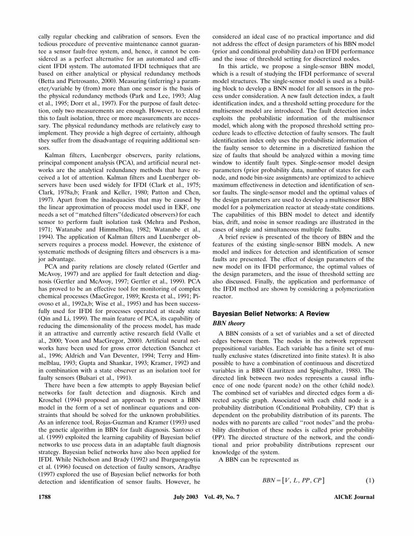
Figure 3. BBN Model III.

Ž .from normal operation is available to describe the correla-tions among the process variables.

� No simultaneous fault types in one sensor. Faults of dif-w Ž .xferent types drift, bias and noise white noise do not occur

simultaneously in one sensor.

Structure of Models IIIModel III, shown in Figure 3, consists of the three dis-

cretized nodes X , R , and B , that are related by the math-a a aematical model

Sensor reading R sActual value X qBias B 3Ž .Ž . Ž . Ž .a a a

Nodes X , B , and R , of Model III have the same defini-a a ations as those of Model I with mutually exclusive states. Todevelop a multisensor BBN model for sensors in a process,

Ž .one needs to connect the single-sensor BBNs models devel-oped using Model III to each other through the X nodesaconsidering the cause-effect relation and the correlation be-tween the X nodes. Node B in Model III plays a key rolea ain performing IFDI, because both detection and identifica-tion of sensor faults by using Model III require analysis ofthe updated state probabilities of node B . While analysis ofaa snapshot data on updated state probabilities of node B isa

Ž .adequate for fault detection task T1 , fault identificationŽ .task T2 requires analysis of the updated state probabilitiesof node B over a sufficiently long period of time.a

Fault DetectionDeviation of state probabilities of node B from their nor-a

Žmal values the values that the probabilities take when there.is no fault is indicative of a fault. Fault detection requires a

method to quantify the deviation. To carry out this systemati-cally, the following two definitions are introduced:

Ž .Definition 1: Probability absolute difference PAD is de-i jfined as the difference between the updated probability of

Ž .state j of node B of sensor i, P B , and the probability ofa a i j�Ž .state j of node B of sensor i in operative mode, P B ,a a i j

both expressed in terms of percentage

�PAD s P B y P B is1, . . . , n , js1, . . . , mŽ . Ž .i j i ji j a a

4Ž .

Definition 2: Sum of probability absolute differences forsensor i, S , isPADi

m

S s PAD is1, . . . , n 5Ž .ÝPAD i jijs1

where n is the number of sensors in a multisensor BBN andm is the number of states of node B .a

For a single-sensor BBN, where ns1, the deviation of thesum of absolute differences from zero is indicative of a fault.However, for a multisensor BBN when faults emerge, be-cause of the correlations among X nodes of sensors, theasum of absolute differences takes a value other than zero evenfor operative sensors. To determine the relative status of a

July 2003 Vol. 49, No. 7 AIChE Journal1790

sensor with respect to other sensors in a multisensor BBN,the following fault detection index for sensor i is introduced:

Definition 3: Fault detection index for sensor i, D is de-ifined as

SPAD iD s100 is1, . . . , n 6Ž .ni

SÝ PAD iis1

This normalized index is basically a percentage of the sum ofthe sum-of-probability-absolute-differences. The index shouldbe used in multisensor IFDI, where n�1. Normalized in-dices have also been used for fault detection elsewhere. For

Ž .example, Qin and Li 1999 defined a normalized index, whichis sensitive to sensor faults that cause variance change. Nor-malization has also been used in calculating sensor validity

Ž .index to measure sensor performance Dunia et al., 1996 .ŽTo achieve effective fault detection no false alarm or

.missed faults , the fault detection index of every sensor in amultisensor BBN should be evaluated using a proper thresh-old-setting procedure. The threshold setting procedure isproposed in the next subsection.

Threshold settingUnivariate or multivariate statistical methods are often

used to determine thresholds for fault detection. While uni-variate statistical methods lack the benefit of using the corre-lations between process variables, the multivariate basedmethods like T 2 statistics incorporate such correlations inthreshold setting, which results in reducing the rate of falsealarms and missed faults. Neither of these two threshold-set-ting methods is applicable to the fault detection index pro-posed in this work. Because of the discrete mode of the nodesof Model III, the updated probabilities of B nodes and alsoathe sum of probability absolute differences do not change aslong as the sensor readings remain within the range of onestate of node R . Therefore, the discrete mode of the nodesaof Model III changes the nature of the sensor readings to theextent that the conventional threshold-setting procedures arenot suitable for fault detection by using Model III. To ex-plain this further, consider a sample of continuous sensorreadings that represent normal operation with a mean of zeroŽ .dimensionless basis and a variance of � . Furthermore, as-sume that the bin range of the state of node R representinga

Ž .normal operation N is set such that it covers the span of � .For the selected bin-range assignment of state N, the up-dated probabilities of node B and, thus, the sum of proba-ability absolute differences do not change, because the evi-

Ž . Ždence state of node R remains unchanged regardless ofa.the value of the sensor reading . To propose a threshold-set-

ting procedure for fault detection by using Model III, halfnumber n is introduced by the following definition.1r2

Ž .Definition 4: The half number n is defined as1r2

n snr2 n is evenŽ .1r27Ž .½ n s ny1 r2 n is oddŽ . Ž .1r2

The outcome of reasoning by using BBN for sensor fault de-tection depends on the number, coherency of evidencesŽ .sensor readings , and correlation among the sensor readings.As an example, analysis of the updated probabilities for faultdetection often points to the group of faulty or operative sen-sors with a number of members exceeding the half numberŽ .n , as the operative group. Therefore, fault detection in1r2cases in which the number of simultaneously-faulty sensorsŽ . Ž .l exceeds the half number n may result in false alarms1r2or missed faults. However, by employing a proper threshold-setting procedure, effective fault detection is feasible in casesthat the number of simultaneously-faulty sensors is less than

Ž .or equal to the half number lFn . To perform effective1r2Ž .fault detection no false alarms or missed faults , the fault

Ž .detection threshold T should be set such thatd

Do �T � Df 8Ž .max d min

where Do is the threshold lower bound, the maximummaxvalue that the fault detection index D takes for operativeisensors. Df is the threshold upper bound, the minimumminvalue that the fault detection index D takes for faulty sen-isors. For the ith sensor in a multisensor BBN, fault detectionis then performed by the simple rule

D �T faulty sensorŽ .i d 9Ž .½ D �T operative sensorŽ .i d

False alarms happen when T � Do , and missed faultsd maxoccur when T � Df . The reliability of the threshold lowerd minand upper bounds depends on the level of uncertainty in the

Žconditional probability data that represents correlations.among X nodes of a multisensor BBN . False alarms anda

missed faults can occur, if conditional probability data usedin a multisensor BBN does not describe accurately correla-tions among X nodes. It is worth noting that the lower theadifference is between threshold lower and upper bounds, thehigher is the probability of false alarms and missed faults. Asthe number of simultaneously-faulty sensors approaches thehalf number, the weight assigned to measurements of faultysensors increases, and, thus, the difference between thresh-old lower and upper bounds decreases to a minimum whenlsn . Cases in which lsn represent the hardest, but1r2 1r2achievable, fault detection task that one could attempt by us-ing BBN. A fault detection threshold, leading to effective faultdetection in these difficult cases, ensures the reliability offault detection for less difficult cases with lFn .1r2

A method of threshold setting can be proposed on the ba-sis of the half number. For a single-sensor BBN with node Raconsisting of m states, the number of possible faulty modes is

Ž .m-1 the one state not included represents normal operation .For a multisensor BBN developed by connecting n of suchsingle-sensor BBNs, the number of possible faulty modes is�w Ž .n1r2 x w Ž . x4n! my1 r n ! nyn ! when lsn . To find a1r2 1r2 1r2fault detection threshold that allows effective fault detectionŽ .no false alarms or missed faults , we propose using the datagenerated for D by simulating faulty modes for which lsni 1r2

July 2003 Vol. 49, No. 7AIChE Journal 1791

to determine the values of threshold lower and upper bounds.The fault detection threshold should then be determined us-ing Eq. 8. The closer is the value of fault detection thresholdto Df or Do , the higher is the probability for missedmin maxfaults or false alarms. The task of threshold setting is basi-cally a compromise between false alarms and missed faults.Such compromise should be done considering the toleranceof a process to false alarms or missed faults.

Fault identificationAfter fault detection in an IFDI procedure, fault identifi-

cation can be carried out for faulty sensors. As mentionedearlier, fault identification using Model III requires analysisof the updated state probabilities of node B over a suffi-aciently long period of time. Such analysis can be carried out

Ž .by using the most probable state MPS and the fault identifi-cation index that are defined below.

Definition 5: The most probable state is the state of nodeB that is most probably responsible for the detected fault.a

Definition 6: Fault identification index for faulty sensor i,I , is defined asi

I smax PAD js1, . . . ,m and j� k 10Ž .Ž .i i jj

where state k is the state representing normal operation.The first step in fault identification is to use the updated

probabilities of node B in a snapshot to determine the mostaprobable state. The state of node B with a probability abso-alute difference equal to the fault identification index is themost probable state. Tracking the status of the most probablestate over a sufficiently long period of time is the second stepthat should lead to fault identification. A time-invariant MPSstatus over a sufficiently long period of time, a steady gradualchange of MPS towards the higher or lower states of bias,and a steady fluctuation of MPS between different states of

Žbias are indications of bias, drift, and noise assumed to be.white noise , respectively. As an example, consider node Ba

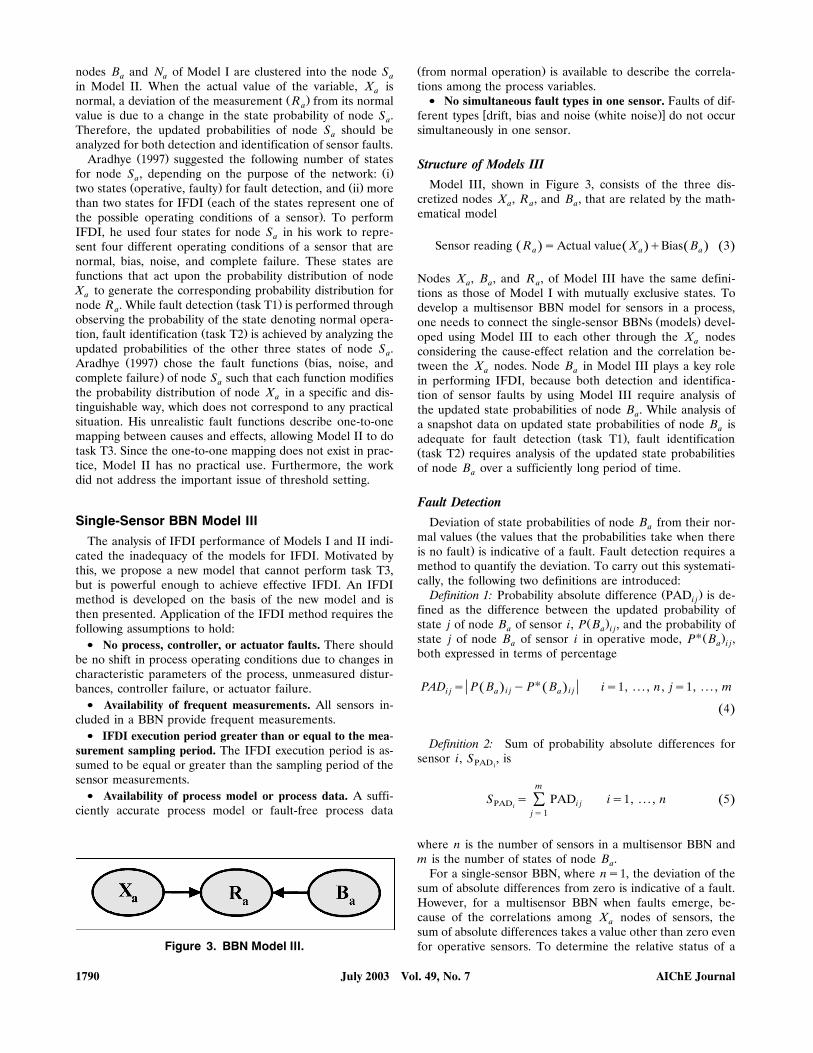
Ž . Ž .with these five states: very negative n2 , negative n1 , zeroŽ . Ž . Ž .z , positive p1 , and very positive p2 , where the state zrepresents normal operation. Figure 4 depicts how the fault

Ž .type bias, drift and noise can be identified for such a nodeB by using Model III. Measurement signals shown in theseafigures by solid lines are filtered sensor readings. The circles

Ž .represent the status of the most probable state MPS that

Figure 4. Identification of bias, drift, and noise by usingModel III.

Figure 5. Polymerization reactor.

changes when the sensor reading crosses the bin-range of thestates. The first section of Figure 4, sampling instance 0 to55, shows two cases of bias in sensor reading. Each case startswith a rapid change followed by biased readings. The rapidchanges are from state z to p2 and then from state p2 to n2,and the biased readings are within the bin-range of the statesp2 and n2. The time-invariance of the MPS status over arelatively long period of time in the first section of Figure 4indicates bias. The sensor reading in the second section ofFigure 4, sampling instance 56 to 130, shows a steady gradualincrease from state z to p2. Such changes in sensor reading,gradual changes towards the higher or lower states of theMPS status, are indicative of a drift. The third section of Fig-ure 4, sampling instance 131 to 150, depicts the way that noisecan be identified. The steady fluctuation of the MPS statusbetween different states of bias indicates noise.

Case study: IFDI using Model IIITo illustrate the application of the fault detection and

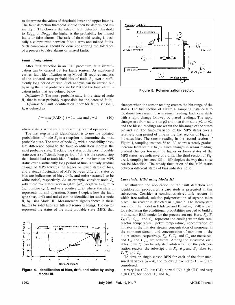
identification procedures, a case study is presented in thissubsection. Consider a continuous-stirred-tank reactor inwhich free-radical, solution polymerization of styrene takesplace. The reactor is depicted in Figure 5. The steady-state

Ž .version of the model in Hidalgo and Brosilow, 1990 is usedfor calculating the conditional probabilities needed to build amultisensor BBN model for the process sensors. Here, F , T ,wT , C , C , and C represent the cooling water flow rate,J ii mm mreactor temperature, jacket temperature, concentration ofinitiator in the initiator stream, concentration of monomer inthe monomer stream, and concentration of monomer in theoutlet stream, respectively. F , T , T , and C are measured,w J mand C and C are constant. Among the measured vari-ii mmables, only F can be adjusted arbitrarily. For the polymer-wization reactor, the subscript a in X , R , and B takes F ,a a a wT , T and C .J m

To develop single-sensor BBN for each of the four mea-Ž . Ž .sured variables ns4 , the following five states ms5 are

considered:� Ž . Ž . Ž . Ž .very low L2 , low L1 , normal N , high H1 and very

Ž .high H2 , for nodes X and R .a a

July 2003 Vol. 49, No. 7 AIChE Journal1792

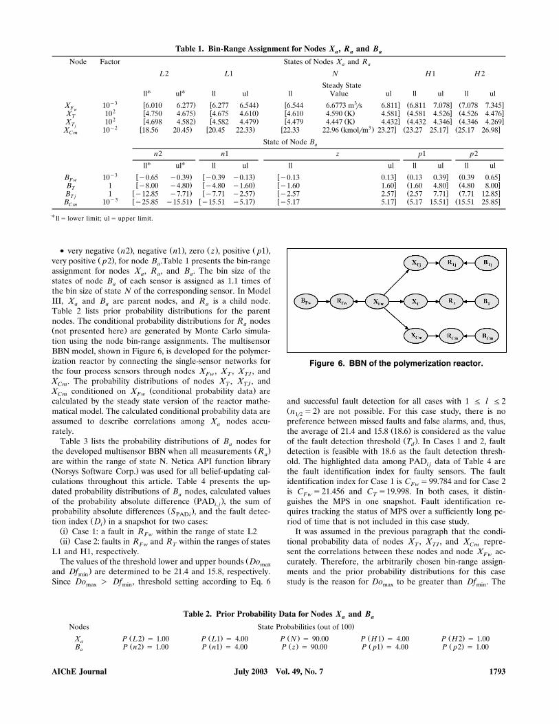
Table 1. Bin-Range Assignment for Nodes X , R and Ba a a

Node Factor States of Nodes X and Ra a

L2 L1 N H1 H2

Steady State� �ll ul ll ul ll Value ul ll ul ll ul

y3 3w . w . w x Ž x Ž xX 10 6.010 6.277 6.277 6.544 6.544 6.6773 mrs 6.811 6.811 7.078 7.078 7.345Fw 2 w . w . w Ž . x Ž x Ž xX 10 4.750 4.675 4.675 4.610 4.610 4.590 K 4.581 4.581 4.526 4.526 4.476T2 w . w . w Ž . x Ž x Ž xX 10 4.698 4.582 4.582 4.479 4.479 4.447 K 4.432 4.432 4.346 4.346 4.269Tj y2 3w . w . w Ž . x Ž x Ž xX 10 18.56 20.45 20.45 22.33 22.33 22.96 kmolrm 23.27 23.27 25.17 25.17 26.98C m

State of Node Ba

n2 n1 z p1 p2� �ll ul ll ul ll ul ll ul ll ul

y3 w . w . w x Ž x Ž xB 10 y0.65 y0.39 y0.39 y0.13 y0.13 0.13 0.13 0.39 0.39 0.65F ww . w . w x Ž x Ž xB 1 y8.00 y4.80 y4.80 y1.60 y1.60 1.60 1.60 4.80 4.80 8.00Tw . w . w x Ž x Ž xB 1 y12.85 y7.71 y7.71 y2.57 y2.57 2.57 2.57 7.71 7.71 12.85T j y3 w . w . w x Ž x Ž xB 10 y25.85 y15.51 y15.51 y5.17 y5.17 5.17 5.17 15.51 15.51 25.85C m

� lls lower limit; uls upper limit.

� Ž . Ž . Ž . Ž .very negative n2 , negative n1 , zero z , positive p1 ,Ž .very positive p2 , for node B .Table 1 presents the bin-rangea

assignment for nodes X , R , and B . The bin size of thea a astates of node B of each sensor is assigned as 1.1 times ofathe bin size of state N of the corresponding sensor. In ModelIII, X and B are parent nodes, and R is a child node.a a aTable 2 lists prior probability distributions for the parentnodes. The conditional probability distributions for R nodesaŽ .not presented here are generated by Monte Carlo simula-tion using the node bin-range assignments. The multisensorBBN model, shown in Figure 6, is developed for the polymer-ization reactor by connecting the single-sensor networks forthe four process sensors through nodes X , X , X , andFw T TJX . The probability distributions of nodes X , X , andCm T TJ

Ž .X conditioned on X conditional probability data areCm Fwcalculated by the steady state version of the reactor mathe-matical model. The calculated conditional probability data areassumed to describe correlations among X nodes accu-arately.

Table 3 lists the probability distributions of B nodes foraŽ .the developed multisensor BBN when all measurements Ra

are within the range of state N. Netica API function libraryŽ .Norsys Software Corp. was used for all belief-updating cal-culations throughout this article. Table 4 presents the up-dated probability distributions of B nodes, calculated valuesa

Ž .of the probability absolute difference PAD , the sum ofi, jŽ .probability absolute differences S , and the fault detec-PAD i

Ž .tion index D in a snapshot for two cases:iŽ .i Case 1: a fault in R within the range of state L2FwŽ .ii Case 2: faults in R and R within the ranges of statesFw T

L1 and H1, respectively.ŽThe values of the threshold lower and upper bounds Domax

.and Df are determined to be 21.4 and 15.8, respectively.minSince Do � Df , threshold setting according to Eq. 6max min

Figure 6. BBN of the polymerization reactor.

and successful fault detection for all cases with 1 F l F2Ž .n s2 are not possible. For this case study, there is no1r2preference between missed faults and false alarms, and, thus,

Ž .the average of 21.4 and 15.8 18.6 is considered as the valueŽ .of the fault detection threshold T . In Cases 1 and 2, faultd

detection is feasible with 18.6 as the fault detection thresh-old. The highlighted data among PAD data of Table 4 arei jthe fault identification index for faulty sensors. The faultidentification index for Case 1 is C s99.784 and for Case 2Fwis C s21.456 and C s19.998. In both cases, it distin-Fw Tguishes the MPS in one snapshot. Fault identification re-quires tracking the status of MPS over a sufficiently long pe-riod of time that is not included in this case study.

It was assumed in the previous paragraph that the condi-tional probability data of nodes X , X , and X repre-T TJ Cmsent the correlations between these nodes and node X ac-Fwcurately. Therefore, the arbitrarily chosen bin-range assign-ments and the prior probability distributions for this casestudy is the reason for Do to be greater than Df . Themax min

Table 2. Prior Probability Data for Nodes X and Ba a

Ž .Nodes State Probabilities out of 100Ž . Ž . Ž . Ž . Ž .X P L2 s 1.00 P L1 s 4.00 P N s 90.00 P H1 s 4.00 P H2 s 1.00aŽ . Ž . Ž . Ž . Ž .B P n2 s 1.00 P n1 s 4.00 P z s 90.00 P p1 s 4.00 P p2 s 1.00a

July 2003 Vol. 49, No. 7AIChE Journal 1793

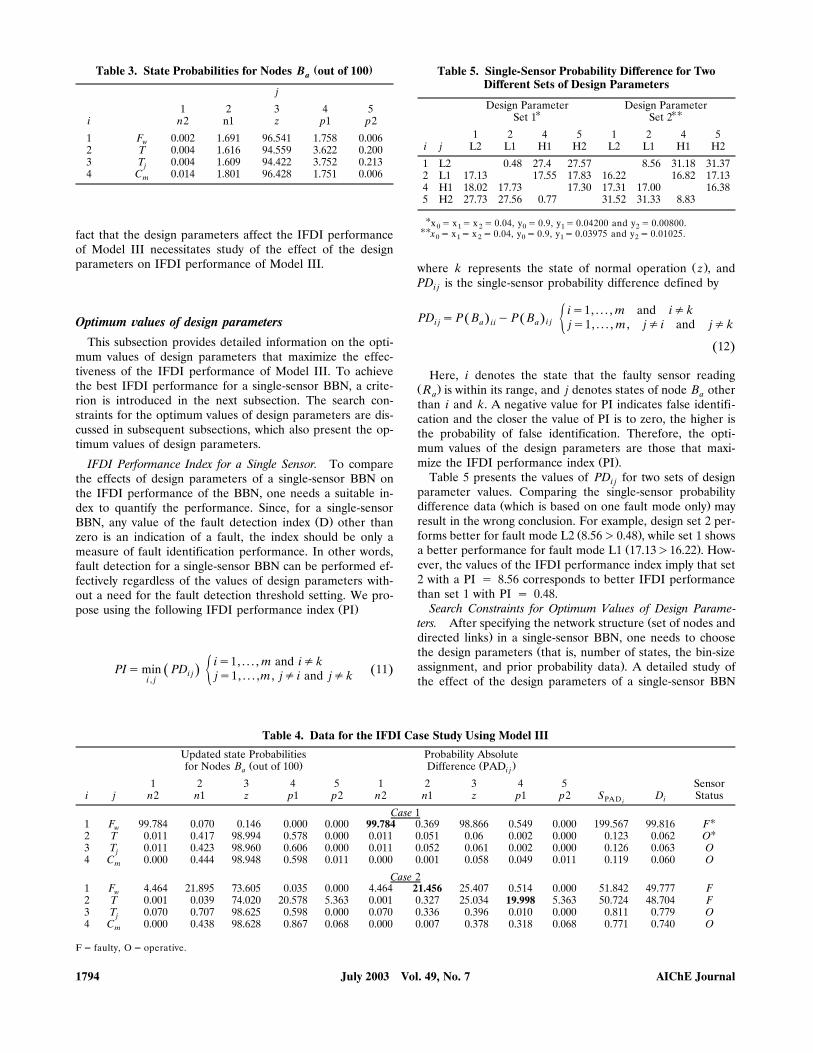
( )Table 3. State Probabilities for Nodes B out of 100a

j

1 2 3 4 5i n2 n1 z p1 p2

1 F 0.002 1.691 96.541 1.758 0.006w2 T 0.004 1.616 94.559 3.622 0.2003 T 0.004 1.609 94.422 3.752 0.213j4 C 0.014 1.801 96.428 1.751 0.006m

fact that the design parameters affect the IFDI performanceof Model III necessitates study of the effect of the designparameters on IFDI performance of Model III.

Optimum ©alues of design parametersThis subsection provides detailed information on the opti-

mum values of design parameters that maximize the effec-tiveness of the IFDI performance of Model III. To achievethe best IFDI performance for a single-sensor BBN, a crite-rion is introduced in the next subsection. The search con-straints for the optimum values of design parameters are dis-cussed in subsequent subsections, which also present the op-timum values of design parameters.

IFDI Performance Index for a Single Sensor. To comparethe effects of design parameters of a single-sensor BBN onthe IFDI performance of the BBN, one needs a suitable in-dex to quantify the performance. Since, for a single-sensor

Ž .BBN, any value of the fault detection index D other thanzero is an indication of a fault, the index should be only ameasure of fault identification performance. In other words,fault detection for a single-sensor BBN can be performed ef-fectively regardless of the values of design parameters with-out a need for the fault detection threshold setting. We pro-

Ž .pose using the following IFDI performance index PI

is1, . . . , m and i� kPIsmin PD 11Ž .Ž .i j ½ js1, . . . ,m , j� i and j� ki , j

Table 5. Single-Sensor Probability Difference for TwoDifferent Sets of Design Parameters

Design Parameter Design Parameter� ��Set 1 Set 2

1 2 4 5 1 2 4 5i j L2 L1 H1 H2 L2 L1 H1 H2

1 L2 0.48 27.4 27.57 8.56 31.18 31.372 L1 17.13 17.55 17.83 16.22 16.82 17.134 H1 18.02 17.73 17.30 17.31 17.00 16.385 H2 27.73 27.56 0.77 31.52 31.33 8.83

�x s x s x s 0.04, y s 0.9, y s 0.04200 and y s 0.00800.0 1 2 0 1 2��x s x s x s 0.04, y s 0.9, y s 0.03975 and y s 0.01025.0 1 2 0 1 2

Ž .where k represents the state of normal operation z , andPD is the single-sensor probability difference defined byi j

is1, . . . , m and i� kPD sP B yP BŽ . Ž . i ji j a aii ½ js1, . . . , m , j� i and j� k

12Ž .

Here, i denotes the state that the faulty sensor readingŽ .R is within its range, and j denotes states of node B othera athan i and k. A negative value for PI indicates false identifi-cation and the closer the value of PI is to zero, the higher isthe probability of false identification. Therefore, the opti-mum values of the design parameters are those that maxi-

Ž .mize the IFDI performance index PI .Table 5 presents the values of PD for two sets of designi j

parameter values. Comparing the single-sensor probabilityŽ .difference data which is based on one fault mode only may

result in the wrong conclusion. For example, design set 2 per-Ž .forms better for fault mode L2 8.56�0.48 , while set 1 shows

Ž .a better performance for fault mode L1 17.13�16.22 . How-ever, the values of the IFDI performance index imply that set2 with a PI s 8.56 corresponds to better IFDI performancethan set 1 with PI s 0.48.

Search Constraints for Optimum Values of Design Parame-Žters. After specifying the network structure set of nodes and

.directed links in a single-sensor BBN, one needs to chooseŽthe design parameters that is, number of states, the bin-size

.assignment, and prior probability data . A detailed study ofthe effect of the design parameters of a single-sensor BBN

Table 4. Data for the IFDI Case Study Using Model III

Updated state Probabilities Probability AbsoluteŽ . Ž .for Nodes B out of 100 Difference PADa i j

1 2 3 4 5 1 2 3 4 5 Sensori j n2 n1 z p1 p2 n2 n1 z p1 p2 S D StatusPAD ii

Case 1�1 F 99.784 0.070 0.146 0.000 0.000 99.784 0.369 98.866 0.549 0.000 199.567 99.816 Fw�2 T 0.011 0.417 98.994 0.578 0.000 0.011 0.051 0.06 0.002 0.000 0.123 0.062 O

3 T 0.011 0.423 98.960 0.606 0.000 0.011 0.052 0.061 0.002 0.000 0.126 0.063 Oj4 C 0.000 0.444 98.948 0.598 0.011 0.000 0.001 0.058 0.049 0.011 0.119 0.060 Om

Case 21 F 4.464 21.895 73.605 0.035 0.000 4.464 21.456 25.407 0.514 0.000 51.842 49.777 Fw2 T 0.001 0.039 74.020 20.578 5.363 0.001 0.327 25.034 19.998 5.363 50.724 48.704 F3 T 0.070 0.707 98.625 0.598 0.000 0.070 0.336 0.396 0.010 0.000 0.811 0.779 Oj4 C 0.000 0.438 98.628 0.867 0.068 0.000 0.007 0.378 0.318 0.068 0.771 0.740 Om

Fs faulty, Os operative.

July 2003 Vol. 49, No. 7 AIChE Journal1794

on the IFDI performance of the model is needed to deducethe search constraints for optimum values of design parame-ters. The conditional probability data of node R of ModelaIII depends on the number of states and the bin-size assign-ment of nodes X , B , and R . One can choose a differenta a a

Ž .number of states for each node Case I or the same numberŽ .of states for all nodes Case II . We propose using the same

number of states for all nodes. The conditional probabilityŽdata of node R is closer to the ideal situation one-to-onea

.mapping between causes and effects in Case II than in CaseI. As a result, Case II allows one to perform fault identifica-tion more effectively. Note that Case II does not impose anylimitations on the status of Model-III nodes. Furthermore,the use of Case II does not affect adversely the IFDI perfor-mance or limit the applicability of Model III.

The bin-size assignment of nodes X , B , and R also af-a a afects the conditional probability data of node R and, thus,athe IFDI performance of Model III. Since node R is theatrue representation of node X for an operative sensor, theabin size of states of node R should be the same as that ofathe corresponding states of node X . Furthermore, accordingato Model III, any deviation from normal sensor reading foran operative sensor is due to the presence of a bias describedby Eq. 1. Equation 1 implies that the size of the states ofnode B should also be the same as that of the correspondingastates of node X . As an example, consider theaparameterrvariable ‘‘a’’ to be represented by a single-sensorBBN consisting of five-state nodes with the same states, asdescribed earlier. On a dimensionless basis, let the bin-range

Ž xassignment of state H1 of node X be 1.1 1.3 and the pa-aŽ .rameterrvariable a be in its ideal status 1.0 . For these con-

ditions, the bin-range of state p1 of node B that causes theaŽ . Žsensor reading R to shift from state N to state H1 is 0.1a

x0.3 . Thus, the bin sizes of states H1 and p1 are both 0.2.The bin-size assignment of nodes X , B , and R has an-a a a

other feature that can be explained by using a property of theŽ .noise fault type . Earlier, it was stated that Model III is ca-

pable of identifying noise, as well as other types of sensorfaults. An important property of the noise is that the distri-bution of the senor reading is usually Gaussian. Therefore,the bin-size assignment of node B should be symmetricaaround the state z; otherwise, effective identification of thenoise is not possible. This discussion on the number of statesand the bin-size assignment of nodes X , B and R can bea a a

Ž .summarized in three rules search constraints :Ž .1 The number of states of nodes X , B , and R shoulda a a

be equal.Ž .2 The bin size of corresponding states of nodes X , B ,a a

and R should be equal.aŽ .3 The bin-size assignment of node B should be symmet-a

ric around the state z. Thus, the number of states of node Bashould be odd.

ŽThese rules for the five-state nodes X , B , and R in aa a a.format that facilitates further discussion are given in Table

6. The notations are defined in the Notation section.More search constraints can be deduced on the basis of

the values that x , x , and x can take. When the measure-0 1 2ment is normalized with respect to its steady-state value, un-der operative noise-free sensor conditions, the steady-statevalue and bias of the measurement are 1 and 0, respectively.Thus, the lower and upper limits for the bin ranges of states

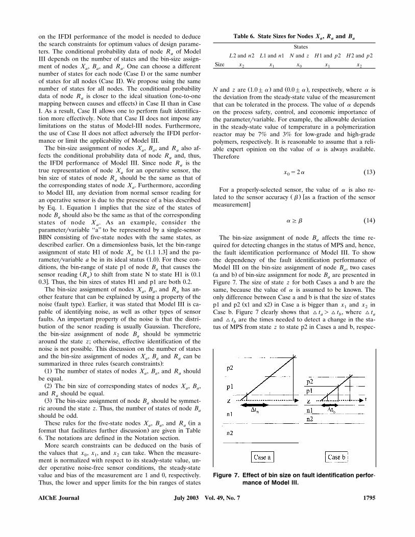
Table 6. State Sizes for Nodes X , R and Ba a a

States

L2 and n2 L1 and n1 N and z H1 and p2 H2 and p2

Size x x x x x2 1 0 1 2

Ž . Ž .N and z are 1.0� � and 0.0� � , respectively, where � isthe deviation from the steady-state value of the measurementthat can be tolerated in the process. The value of � dependson the process safety, control, and economic importance ofthe parameterrvariable. For example, the allowable deviationin the steady-state value of temperature in a polymerizationreactor may be 7% and 3% for low-grade and high-gradepolymers, respectively. It is reasonable to assume that a reli-able expert opinion on the value of � is always available.Therefore

x s2� 13Ž .0

For a properly-selected sensor, the value of � is also re-Ž . wlated to the sensor accuracy � as a fraction of the sensor

xmeasurement

�G� 14Ž .

The bin-size assignment of node B affects the time re-aquired for detecting changes in the status of MPS and, hence,the fault identification performance of Model III. To showthe dependency of the fault identification performance ofModel III on the bin-size assignment of node B , two casesaŽ .a and b of bin-size assignment for node B are presented inaFigure 7. The size of state z for both Cases a and b are thesame, because the value of � is assumed to be known. Theonly difference between Case a and b is that the size of states

Ž .p1 and p2 x1 and x2 in Case a is bigger than x and x in1 2Case b. Figure 7 clearly shows that ^ t �^ t , where ^ ta b aand ^ t are the times needed to detect a change in the sta-btus of MPS from state z to state p2 in Cases a and b, respec-

Figure 7. Effect of bin size on fault identification perfor-mance of Model III.

July 2003 Vol. 49, No. 7AIChE Journal 1795

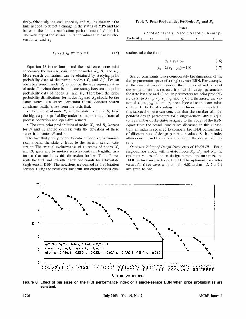
tively. Obviously, the smaller are x and x , the shorter is the1 2time needed to detect a change in the status of MPS and thebetter is the fault identification performance of Model III.The accuracy of the sensor limits the values that can be cho-sen for x and x1 2

x , x F x , when �s� 15Ž .1 2 0

Equation 15 is the fourth and the last search constraintconcerning the bin-size assignment of nodes X , B , and R .a a aMore search constraints can be obtained by studying prior

Ž .probability data of the parent nodes X and B . For ana aoperative sensor, node R cannot be the true representativeaof node X , when there is an inconsistency between the prioraprobability data of nodes X and B . Therefore, the priora aprobability distributions for nodes X and B should be thea a

Ž .same, which is a search constraint fifth . Another searchŽ .constraint sixth arises from the facts that:

� The state N of node X and the state z of node B havea aŽthe highest prior probability under normal operation normal

.process operation and operative sensor .� ŽThe state prior probabilities of nodes X and B excepta a

.for N and z should decrease with the deviation of thesestates from states N and z.

The fact that prior probability data of node B is symmet-arical around the state z leads to the seventh search con-straint. The mutual exclusiveness of all states of nodes Xa

Ž .and B gives rise to another search constraint eighth . In aaformat that facilitates this discussion further, Table 7 pre-sents the fifth and seventh search constraints for a five-statesingle-sensor BBN. The notations are defined in the Notationsection. Using the notations, the sixth and eighth search con-

Table 7. Prior Probabilities for Nodes X and Ba a

States

L2 and n2 L1 and n1 N and z H1 and p2 H2 and p2

Probability y y y y y2 1 0 1 2

straints take the forms

y � y � y 16Ž .0 1 2

y q2 y q y s100 17Ž . Ž .0 1 2

Search constraints lower considerably the dimension of thedesign parameter space of a single-sensor BBN. For example,in the case of five-state nodes, the number of independent

Ždesign parameters is reduced from 25 15 design parametersfor state bin size and 10 design parameters for prior probabil-

. Ž .ity data to 5 x , x , y , y , and y . Furthermore, the val-1 2 0 1 2ues of x , x , y , y , and y are subjected to the constraints1 2 0 1 2of Eqs. 15 to 17. According to the discussion presented inthis subsection, one can conclude that the number of inde-pendent design parameters for a single-sensor BBN is equalto the number of the states assigned to the nodes of the BBN.Apart from the search constraints discussed in this subsec-tion, an index is required to compare the IFDI performanceof different sets of design parameter values. Such an indexallows one to find the optimum value of the design parame-ters.

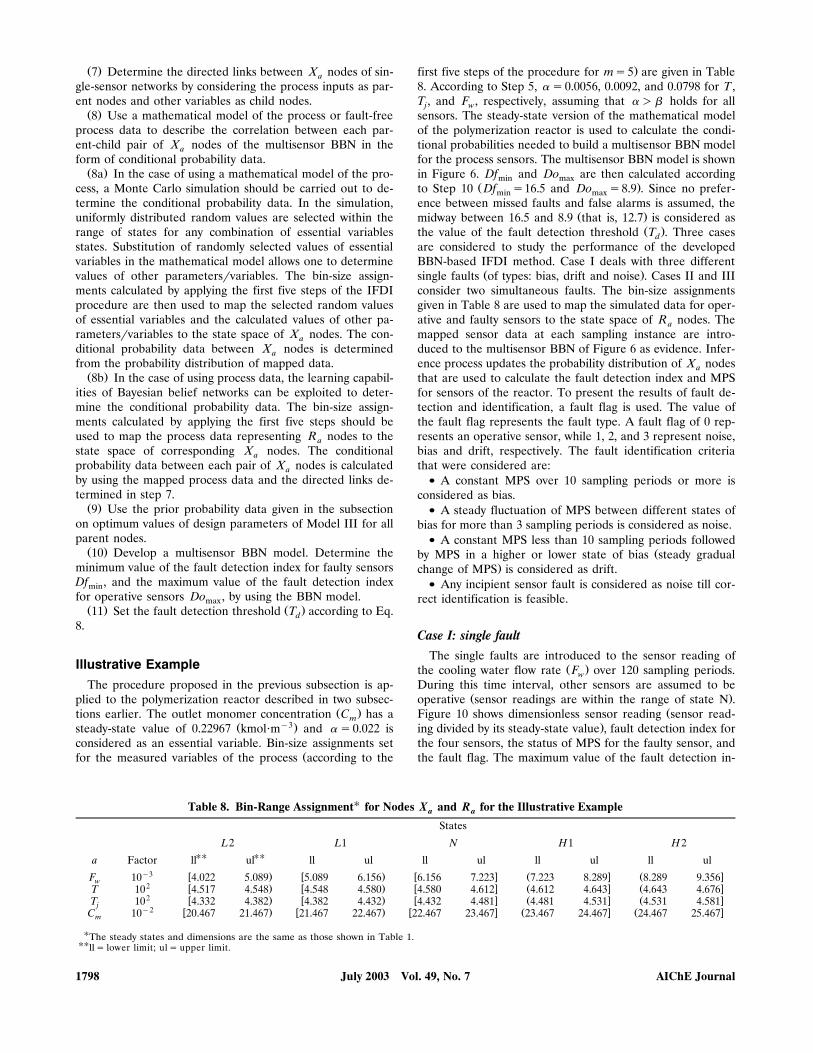
Optimum Values of Design Parameters of Model III. For asingle-sensor model with m-state nodes X , B , and R , thea a aoptimum values of the m design parameters maximize theIFDI performance index of Eq. 11. The optimum parametervalues for three cases with �s�s0.02 and ms5, 7 and 9are given below:

Figure 8. Effect of bin sizes on the IFDI performance index of a single-sensor BBN when prior probabilities areconstant.

July 2003 Vol. 49, No. 7 AIChE Journal1796

Ž . Ž .1 When the prior probabilities y , y , y , . . . are con-0 1 2stant, the IFDI performance index increases as the bin sizesŽ .x , x , . . . increase. This trend is shown in Figure 8 for the1 2case with ms5 and x s2�s0.04. This fact and the con-0straint of Eq. 15 leads to the conclusion that the best IFDIperformance is achievable when the bin sizes of all states areequal to x .0Ž .2 For the cases in which the bin sizes of all states are

equal to x , the prior probabilities that maximize the IFDI0performance index are:Ž .a ms5: y s75.0, y s7.88, y s4.620 1 2Ž .b ms7: y s75.0, y s6.33, y s3.88, y s2.290 1 2 3Ž .c ms9: y s74.0, y s5.87, y s3.52, y s2.21, y s1.400 1 2 3 4

Ž .The prior probability assignment 4, d that maximizes theperformance index is shown in Figure 9 for the case of five-state nodes with x s x s x s0.04. These were obtained by0 1 2a systematic search among all possible values for prior proba-bilities subject to the constraints of Eqs. 16 and 17.

Procedure for IFDIMaintaining essential variables of a continuous process

within acceptable ranges ensures a satisfactory operation ofthe process at steady state. To achieve an effective IFDI, theacceptable range of every essential variable should be consid-ered in bin-size assignment of a BBN model. In view of thisand the results on the optimum design parameters andthreshold setting, the following procedure for IFDI by ModelIII is proposed:Ž .1 Determine the steady-state values and the acceptable

Žrange of the essential variables those that should be moni-.tored andror controlled to ensure a satisfactory operation .

Ž .2 For each essential variable, determine the bin range ofŽ .the state N x s2� of node X on the basis of the accept-0 a

able range of the essential variable. Different bin ranges maybe assigned for different essential variables.Ž . Ž .3 Select a value for the number of states m such that

the total range of interest can be covered for each essentialvariable. This value should be the same for all essential vari-ables. The upper and lower limits of the total range for eachessential variable can be determined from

Upper and lower limitssSteady state ®alue� m� 18Ž . Ž .

Ž .4 Determine the upper and lower limits of other parame-Ž .tersrvariables by using i a mathematical model of the pro-

Ž . Ž .cess or process data if available , and ii the upper and lowerlimits of the essential variables.Ž . Ž .5 Divide the total range from step 4 by the number of

Ž . Ž .states m, from step 3 to get the state bin size x for pro-0cess variables other than essential variables. Note that for aproperly selected sensor

x0 i� G� and � s is l , . . . ,n 19Ž .i i i 2

Žwhere n is the number of measurable variables sensors re-.quired in a multisensor BBN . Any sensor that does not meet

the requirement of Eq. 19, may cause a false alarm.Ž . Ž .6 Use the bin-size assignment from the previous steps

in a Monte Carlo simulation to calculate the necessary condi-tional probability data for single-sensor networks.

Figure 9. Effect of prior probabilities on the IFDI performance index of a single-sensor BBN when bin sizes areconstant.

July 2003 Vol. 49, No. 7AIChE Journal 1797

Ž .7 Determine the directed links between X nodes of sin-agle-sensor networks by considering the process inputs as par-ent nodes and other variables as child nodes.Ž .8 Use a mathematical model of the process or fault-free

process data to describe the correlation between each par-ent-child pair of X nodes of the multisensor BBN in theaform of conditional probability data.Ž .8a In the case of using a mathematical model of the pro-

cess, a Monte Carlo simulation should be carried out to de-termine the conditional probability data. In the simulation,uniformly distributed random values are selected within therange of states for any combination of essential variablesstates. Substitution of randomly selected values of essentialvariables in the mathematical model allows one to determinevalues of other parametersrvariables. The bin-size assign-ments calculated by applying the first five steps of the IFDIprocedure are then used to map the selected random valuesof essential variables and the calculated values of other pa-rametersrvariables to the state space of X nodes. The con-aditional probability data between X nodes is determinedafrom the probability distribution of mapped data.Ž .8b In the case of using process data, the learning capabil-

ities of Bayesian belief networks can be exploited to deter-mine the conditional probability data. The bin-size assign-ments calculated by applying the first five steps should beused to map the process data representing R nodes to theastate space of corresponding X nodes. The conditionalaprobability data between each pair of X nodes is calculatedaby using the mapped process data and the directed links de-termined in step 7.Ž .9 Use the prior probability data given in the subsection

on optimum values of design parameters of Model III for allparent nodes.Ž .10 Develop a multisensor BBN model. Determine the

minimum value of the fault detection index for faulty sensorsDf , and the maximum value of the fault detection indexminfor operative sensors Do , by using the BBN model.maxŽ . Ž .11 Set the fault detection threshold T according to Eq.d

8.

Illustrative ExampleThe procedure proposed in the previous subsection is ap-

plied to the polymerization reactor described in two subsec-Ž .tions earlier. The outlet monomer concentration C has am

Ž y3.steady-state value of 0.22967 kmol�m and �s0.022 isconsidered as an essential variable. Bin-size assignments set

Žfor the measured variables of the process according to the

.first five steps of the procedure for ms5 are given in Table8. According to Step 5, �s0.0056, 0.0092, and 0.0798 for T ,T , and F , respectively, assuming that � � � holds for allj wsensors. The steady-state version of the mathematical modelof the polymerization reactor is used to calculate the condi-tional probabilities needed to build a multisensor BBN modelfor the process sensors. The multisensor BBN model is shownin Figure 6. Df and Do are then calculated accordingmin max

Ž .to Step 10 Df s16.5 and Do s8.9 . Since no prefer-min maxence between missed faults and false alarms is assumed, the

Ž .midway between 16.5 and 8.9 that is, 12.7 is considered asŽ .the value of the fault detection threshold T . Three casesd

are considered to study the performance of the developedBBN-based IFDI method. Case I deals with three different

Ž .single faults of types: bias, drift and noise . Cases II and IIIconsider two simultaneous faults. The bin-size assignmentsgiven in Table 8 are used to map the simulated data for oper-ative and faulty sensors to the state space of R nodes. Theamapped sensor data at each sampling instance are intro-duced to the multisensor BBN of Figure 6 as evidence. Infer-ence process updates the probability distribution of X nodesathat are used to calculate the fault detection index and MPSfor sensors of the reactor. To present the results of fault de-tection and identification, a fault flag is used. The value ofthe fault flag represents the fault type. A fault flag of 0 rep-resents an operative sensor, while 1, 2, and 3 represent noise,bias and drift, respectively. The fault identification criteriathat were considered are:

� A constant MPS over 10 sampling periods or more isconsidered as bias.

� A steady fluctuation of MPS between different states ofbias for more than 3 sampling periods is considered as noise.

� A constant MPS less than 10 sampling periods followedŽby MPS in a higher or lower state of bias steady gradual

.change of MPS is considered as drift.� Any incipient sensor fault is considered as noise till cor-

rect identification is feasible.

Case I: single faultThe single faults are introduced to the sensor reading of

Ž .the cooling water flow rate F over 120 sampling periods.wDuring this time interval, other sensors are assumed to be

Ž .operative sensor readings are within the range of state N .ŽFigure 10 shows dimensionless sensor reading sensor read-

.ing divided by its steady-state value , fault detection index forthe four sensors, the status of MPS for the faulty sensor, andthe fault flag. The maximum value of the fault detection in-

Table 8. Bin-Range Assignment� for Nodes X and R for the Illustrative Examplea a

States

L2 L1 N H1 H2�� ��a Factor ll ul ll ul ll ul ll ul ll ul

y3 w . w . w x Ž x Ž xF 10 4.022 5.089 5.089 6.156 6.156 7.223 7.223 8.289 8.289 9.356w2 w . w . w x Ž x Ž xT 10 4.517 4.548 4.548 4.580 4.580 4.612 4.612 4.643 4.643 4.6762 w . w . w x Ž x Ž xT 10 4.332 4.382 4.382 4.432 4.432 4.481 4.481 4.531 4.531 4.581j y2 w . w . w x Ž x Ž xC 10 20.467 21.467 21.467 22.467 22.467 23.467 23.467 24.467 24.467 25.467m

�The steady states and dimensions are the same as those shown in Table 1.��lls lower limit; uls upper limit.

July 2003 Vol. 49, No. 7 AIChE Journal1798

( )Figure 10. IFDI when a single fault drift, bias or noiseis present: Case I.

Ž .dex for the T , T , and C sensors operative sensors is 1.95.j mThe minimum value of the fault detection index for the Fw

Ž .sensor faulty sensor is 95.75 when the fault is present. TheŽ .assigned value for fault detection threshold 12.7 , and the

considerable difference between 1.95 and 95.75 allow effec-tive fault detection without delay. Table 9 presents the startand end time instants for each fault type and the time instantof each correct identification. The effect of the fault identifi-

Ž .cation criteria listed in the previous subsection on identifi-cation time delay is clearly reflected in the data presented inTable 9. As can be seen, there is no identification time delayfor the noise fault, and the maximum identification time de-

Ž .lay is for the drift fault 9 sampling periods . There are twonormal sensor readings during the occurrence of the noisefault. These normal sensor readings cause the identificationtime delay for the noise fault to be five sampling instants.

Table 9. Starting Time Instant of Faults and Fault Identifi-cation Time Instant in Case I of the Illustrative Example

Fault Type

Time Instant Drift Bias Noise

Start 26 39 90Identification 35 44 95

Figure 11. IFDI when two simultaneous bias faults arepresent: Case II.

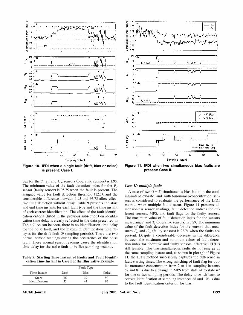
Case II: multiple faultsŽ .A case of two ls2 simultaneous bias faults in the cool-

ing-water-flow-rate and outlet-monomer-concentration sen-sors is considered to evaluate the performance of the IFDImethod when multiple faults occur. Figure 11 presents di-mensionless sensor readings, fault detection indices for dif-ferent sensors, MPS, and fault flags for the faulty sensors.The maximum value of fault detection index for the sensors

Ž .measuring T and T operative sensors is 7.29. The minimumjvalue of the fault detection index for the sensors that mea-

Ž .sures F and C faulty sensors is 22.71 when the faults arew mpresent. Despite a considerable decrease in the differencebetween the maximum and minimum values of fault detec-tion index for operative and faulty sensors, effective IFDI isstill feasible. The two simultaneous faults do not emerge at

Ž .the same sampling instant and, as shown in plot g of Figure11, the IFDI method successfully captures the difference infault starting times. The wrong switching of fault flag for out-let monomer concentration from 2 to 1 at sampling instants57 and 81 is due to a change in MPS from state n1 to state n2for one or two sampling periods. The delay to switch back tocorrect identification at sampling instances 68 and 106 is dueto the fault identification criterion for bias.

July 2003 Vol. 49, No. 7AIChE Journal 1799

Figure 12. IFDI when two simultaneous bias and preci-sion-degradation faults are present: Case III.

Case III: multiple faultsŽ .Another case of two ls2 simultaneous faults in the reac-

tor-temperature and outlet-monomer-concentration sensors isalso presented here to show the capabilities of the developedIFDI method in detecting and identifying multiple faults ofdifferent types. The fault types are bias and noise for thesensors. The result of IFDI for this case is presented in Fig-ure 12. The maximum value of the fault detection index for

Ž .the T and F sensors that are operative sensors is 5.26.j wThe minimum value of fault detection index for the sensors

Ž .that measures T and C faulty sensors is 33.40 when themfaults are present. The difference between the maximum andminimum value of fault detection index for operative and

Ž .faulty sensors and the value of fault detection threshold 12.7allow effective IFDI. As can be seen in Figure 12, the dissim-ilarity of fault types is not a limitation for an effective IFDIby the method.

ConclusionsA single-sensor BBN model was proposed. In contrast to

the existing models, it has the capabilities needed to carry

out a complete IFDI. The IFDI performance of the modelwas studied, and the optimum values of the design parame-ters that make effective fault detection and identificationpossible were given. A multisensor, BBN-based IFDI methodwas developed. The necessity of a new approach of thresholdsetting for the developed IFDI method was discussed, andsuch an approach was presented. Guidelines were presentedto facilitate the application of the developed method, and theillustrative examples were given to show the performance ofthe method. The examples showed that the method is capa-ble of detecting single and multiple sensor faults, and identi-

Ž .fying the three fault types bias, drift, and noise . While capa-ble of identifying the three fault types, the developed methodcannot identify sensor complete failure.

The application of BBN in IFDI presented here revealedsome potentials of BBN. More studies are needed to exploreother potentials of BBN. Future work includes extending themethod to transient processes, and investigating the possibil-ity of performing process fault detection and diagnosis alongwith IFDI. Frequency of fault types I and II is a good mea-sure of the efficiency of an IFDI method. Future work alsoincludes conducting simulations and applying this BBN-based

Žand the other IFDI methods such as those that are based on.PCA and Kalman filtering to industrial processes to deter-

mine relative advantages and disadvantages of the IFDImethods.

NotationAsun-instantiated prepositional variableasparameterrvariable that is measured

B snode representing the bias associated with Xa aC sconcentration of initiator in the initiator inlet streami i

Ž y3 .kmol �mŽC sconcentration of monomer in the outlet stream kmol�m y3 .m

C sconcentration of monomer in the monomer inlet streammmŽ y3 .kmol�m

CPsconditional probability distribution of child nodes in aBBN

Df sminimum of fault detection indices of faulty sensorsminD s fault detection index of sensor ii

Do smaximum of fault detection indices of operative sensorsmaxŽ .Es instantiated prepositional variable evidence

Ž 3 -1.F scooling water flow rate m �swH1sstate of nodes R and X representing the actual value ofa a

the parameterrvariable a and the available measurementin the range of high

H2sstate of nodes R and X representing the actual value ofa athe parameterrvariable a and the available measurementin the range of very high

I s fault identification index of sensor iiLsset of directed links in a BBNlsnumber of simultaneously-faulty sensors in a multisensor

BBNL1sstate of nodes R and X representing the actual value ofa a

the parameterrvariable a and the available measurementin the range of low

L2sstate of nodes R and X representing the actual value ofa athe parameterrvariable a and the available measurementin the range of very low

msnumber of states for each node in a multisensor BBNŽMPSsmost probable state state of node B that is most proba-a

.bly responsible for the detected faultnsnumber of sensors in a multisensor BBN

July 2003 Vol. 49, No. 7 AIChE Journal1800

Nsstate of nodes R and X representing normal conditiona afor actual value of the parameterrvariable a and availablemeasurement

n shalf number1r2n1sstate of node B representing bias in the range of nega-a

tiven2sstate of node B representing bias in the range of verya

negativeN snode representing the noise associated with Xa aPsstate probability of a prepositional variable

P�s state probability of a prepositional variable in operativemode

p1sstate of node B representing bias in the range of positiveap2sstate of node B representing bias in the range of verya

positivePAD sprobability absolute difference of state j of sensor ii j

PPsprior probability distribution of parent nodes in a BBNR snode representing the available measurement for Xa a

S ssum of probability absolute differences of sensor iPAD i

Tsreactor temperature, KT s fault detection thresholddTs jacket temperature, KjVsset of variables or nodes in a BBNx sbin size of the state N of nodes R and X , and state z of0 a a

node Bax sbin size of the states L1 and H1 of nodes R and X , and1 a a

states n1 and p1 of node Bax sbin size of the states L2 and H2 of nodes R and X , and2 a a

states n2 and p2 of node BaX snode representing the actual value of the parameterrvari-a

able ay sprior probability of state N of node X , and state z of0 a

node Bay sprior probability of state L1 of node X , and state n1 of1 a

node Bay sprior probability of state L2 of node X , and state n2 of2 a

node Bazsstate of node B representing zero biasa

Greek letters�sacceptable deviation of a parameterrvariable from its

steady-state valueŽ .�ssensor accuracy fraction of the sensor reading

� t s time needed to detect a change in the status of MPS foraCase a of Figure 7

� t s time needed to detect a change in the status of MPS forbCase b of Figure 7

�sstandard deviation of a sensor reading sample

Literature CitedAlag, S., K. Goebel, and A. Agogino, ‘‘A Methodology for Intelligent

Sensor Validation and Fusion used in Tracking and Avoidance ofObjects for Automated Vehicles,’’ Proc. of Amer. Contr. Conf.,

Ž .Seattle, WA, 3647 1995 .Aldrich, C., and J. S. J. Van Deventer, ‘‘Identification of Gross Er-

rors in Material Balance Measurements by Means of Neural Nets,’’Ž .Chem. Eng. Sci., 49, 1357 1994 .

Aradhye, H. B., ‘‘Sensor Fault Detection, Isolation, and Accommo-dation Using Neural Networks, Fuzzy Logic, and Bayesian BeliefNetworks,’’ M.S. Diss., University of New Mexico, Albuquerque,

Ž .NM 1997 .Betta, G., and A. Pietrosanto, ‘‘Instrument Fault Detection and Iso-

lation: State of the Art and New Research Trends,’’ IEEE Trans.Ž .Instr. and Meas., 49, 100 2000 .

Bulsari, A., A. Medvedev, and H. Saxen, ‘‘Sensor Fault DetectionUsing State Vector Estimator and Feed-Forward Neural NetworksApplied to a Simulated Biochemical Process,’’ Acta Polytech.

Ž .Scand., Chem. Technol. Metall. Ser., 20, 199 1991 .Clark, R. N., ‘‘Instrument fault detection,’’ IEEE Trans. Aerosp. Elec-

Ž .tron. Syst., 14, 456 1978a .Clark, R. N., ‘‘A Simplified Instrument Failure Detection Scheme,’’

Ž .IEEE Trans. Aerosp. Electron. Syst., 14, 558 1978b .

Clark, R. N., D. C. Fosth, and V. M. Walton, ‘‘Detection InstrumentMalfunction in Control Systems,’’ IEEE Trans. Aerosp. Electron.

Ž .Syst., 11, 465 1975 .Dorr, R., F. Kratz, J. Ragot, F. Loisy, and J. L. Germain, ‘‘Detec-

tion, Isolation, and Identification of Sensor Faults in NuclearŽ .Power Plants,’’ IEEE Trans. Contr. Syst. Techn., 5, 42 1997 .

Dunia, R., S. J. Qin, T. F. Edgar and T. J. McAvoy, ‘‘Identificationof Faulty Sensors Using Principal Component Analysis,’’ AIChE J.,

Ž .42, 2797 1996 .Frank, P. M., and L. Keller, ‘‘Sensitivity Discriminating Observer

Design for Instrument Failure Detection,’’ IEEE Trans. Aerosp.Ž .Electron. Syst., 16, 456 1980 .

Gertler, J. J., and T. J. McAvoy, ‘‘Principal Component Analysis andParity Relations-A Strong Duality,’’ IFAC SAFEPROCESS Symp.,

Ž .2, 837 1997 .Gertler, J. J., W. Li, Y. Huang, and T. J. McAvoy, ‘‘Isolation En-

Ž .hanced Principal Component Analysis,’’ AIChE J., 29, 243 1999 .Gupta, G., and N. Shankar, ‘‘Application of Neural Networks for

Ž .Gross Error Detection,’’ Ind. Eng. Chem. Res., 32, 1651 1993 .Hidalgo, P. M., and C. B. Brosilow, ‘‘Nonlinear Model Predictive

Control of Styrene Polymerization at Unstable Operating Points,’’Ž .Comput. Chem. Eng., 14, 481 1990 .

Ibarguengoytia, P. H., L. E. Sucar, and S. Vadera, ‘‘A ProbabilisticModel for Sensor Validation,’’ Proc. Conf. on Uncertainty in Artifi-

Ž .cial Intelligence, Portland, OR, 332 1996 .Kirch, H., and K. Kroschel, ‘‘Applying Bayesian Networks to Fault

Ž .Diagnosis,’’ Proc. of IEEE Conf. on Control Applications, 895 1994 .Kramer, M. A., ‘‘Autoassociative Neural Networks,’’ Comput. Chem.

Ž .Eng., 16, 313 1992 .Kresta, J. V., J. F. MacGregor, and T. E. Marlin, ‘‘Multivariate Sta-

Ž .tistical Monitoring of Processes,’’ Can. J. Chem. Eng., 69 35 1991 .Lauritzen, S. L., and D. J. Spieglhalter, ‘‘Local Computation with

Probabilities on Graphical Structures and Their Application to Ex-Ž .pert Systems,’’ J. Roy. Stat. Soc., B, 50, 157 1988 .

Lee, W. Y., J. M. House, and D. R. Shin, ‘‘Fault Diagnosis and Tem-perature Sensor Recovery for an Air-Handling Unit,’’ ASHRAE

Ž .Trans., 103 621 1997 .MacGregor, J. F., ‘‘Multivariate Statistical Methods for Monitoring

Large Databases from Chemical Processes,’’ AIChE Meeting, SanŽ .Francisco 1989 .

Mehra, R. K., and I. Peshon, ‘‘An Innovations Approach to FaultDetection and Diagnosis in Dynamic Systems,’’ Automatica, 7, 637Ž .1971 .

Nicholson, A. E., and J. M. Brady, ‘‘Sensor Validation Using Dy-namic Belief Networks,’’ Proc. of 8th Conf. on Uncertainty in Artifi.

Ž .Intell., 207 1992 .Park, S., and C. S. G. Lee, ‘‘Fusion-Based Sensor Fault Detection,’’

Ž .Proc. of Int. Symp. on Intelligent Contr., Chicago, 156 1993 .Patton, R. J. and J. Chen, ‘‘Observer-Based Fault Detection and Iso-

lation: Robustness and Applications,’’ Control Eng. Practice, 5, 671Ž .May 1997 .

Piovoso, M. J., K. A. Kosanovich, and P. K. Pearson, ‘‘MonitoringProcess Performance in Real Time,’’ Proc. Amer. Control Conf.,

Ž .Chicago, 2359 1992a .Piovoso, M. J., K. A. Kosanovich, and J. P. Yuk, ‘‘Process Data

Ž .Chemometrica,’’ IEEE Trans. Instr. and Meas., 41, 262 1992b .Qin, S. J. and W. Li, ‘‘Detection, Identification, and Reconstruction

Ž .of Faulty Sensors with Maximized Sensitivity,’’ AIChE J., 45 9 ,Ž .1813 1999 .

Rojas-Guzman, C., and M. A. Kramer, ‘‘Comparison of Belief Net-works and Rule-based Expert Systems for fault Diagnosis of

Ž .Chemical,’’ Eng. Applic. Artif. Intell., 6, 191 1993 .Sanchez, M., G. Sentoni, S. Schbib, S. Tonelli, and J. Romagnoli,

‘‘Gross Measurements Error DetectionrIdentification for an In-Ž .dustrial Ethylene Reactor,’’ Comput. Chem. Eng., 20 972 , S1559

Ž .1996 .Santoso, N. I., C. Darken, and G. Povh, ‘‘Nuclear Plant Fault Diag-

nosis Using Probabilistic Reasoning,’’ Power Eng. Soc. SummerŽ .Meeting, IEEE, 2, 714 1999 .

Terry, P. A., and D. M. Himmelblau, ‘‘Data Rectification and GrossError Detection in a Steady-State Process Via Artificial Neural

Ž .Networks,’’ Ind. Eng. Chem. Res., 32, 3020 1993 .Valle, S., J. S. Qin, and M. J. Piovoso, ‘‘Analysis of Multi-Block PCA

and PLS for Fault Detection and Identification,’’ AIChE Meeting,Ž .Los Angeles 2000 .

July 2003 Vol. 49, No. 7AIChE Journal 1801

Watanabe, K., and D. M. Himmelblau, ‘‘Instrument Fault DetectionŽ .in Systems with Uncertainties,’’ Int. J. Syst. Sci., 13, 73 1982 .

Watanabe, K., A. Komori, and T. Kiyama, ‘‘Diagnosis of InstrumentŽ .Fault,’’ Proc. IEEE IMTC, Hamamatsu, Japan, 386 1994 .

Wise, B. M., N. B. Gallagher, and J. F. MacGregor, ‘‘The ProcessChemometrics Approach to Process Monitoring and Fault Detec-tion,’’ Proc. IFAC Workshop on On-Line Fault Detection and Super-

Ž .®ision in the Chemical Industries, Newcastle, U.K., 1 1995 .

Yoon, S., and J. F. MacGregor, ‘‘PCA of Multiscale Data and itsApplication to Fault Isolation,’’ AIChE Meeting, Los AngelesŽ .2000 .

Manuscript recei®ed June 28, 2002, and re®ision recei®ed Feb. 4, 2003.

July 2003 Vol. 49, No. 7 AIChE Journal1802