Utah State University Utah State University

DigitalCommons@USU DigitalCommons@USU

All Graduate Theses and Dissertations Graduate Studies

8-2011

A Thermomechanical Analysis of An Ultrasonic Bonding A Thermomechanical Analysis of An Ultrasonic Bonding

Mechanism Mechanism

Chunbo Zhang Utah State University

Follow this and additional works at: https://digitalcommons.usu.edu/etd

Part of the Mechanical Engineering Commons

Recommended Citation Recommended Citation Zhang, Chunbo, "A Thermomechanical Analysis of An Ultrasonic Bonding Mechanism" (2011). All Graduate Theses and Dissertations. 1021. https://digitalcommons.usu.edu/etd/1021

This Dissertation is brought to you for free and open access by the Graduate Studies at DigitalCommons@USU. It has been accepted for inclusion in All Graduate Theses and Dissertations by an authorized administrator of DigitalCommons@USU. For more information, please contact digitalcommons@usu.edu.

A THERMOMECHANICAL ANALYSIS OF AN ULTRASONIC BONDING

MECHANISM

by

Chunbo (Sam) Zhang

A dissertation submitted in partial fulfillmentof the requirements for the degree

of

DOCTOR OF PHILOSOPHY

in

Mechanical Engineering

Approved:

Dr. Leijun Li Dr. Robert E. SpallMajor Professor Committee Member

Dr. Barton Smith Dr. Brent StuckerCommittee Member Committee Member

Dr. Wei Ren Dr. Mark R. McLellanCommittee Member Vice President for Research and

Dean of the School of Graduate Studies

UTAH STATE UNIVERSITYLogan, Utah

2011

ii

Copyright c© Chunbo (Sam) Zhang 2011

All Rights Reserved

iii

Abstract

A Thermomechanical Analysis of An Ultrasonic Bonding Mechanism

by

Chunbo (Sam) Zhang, Doctor of Philosophy

Utah State University, 2011

Major Professor: Dr. Leijun LiDepartment: Mechanical and Aerospace Engineering

A systematic experimental and numerical combined study of the thermomechanical

bonding mechanisms in the ultrasonic welding (UW) process was conducted. A fully cou-

pled thermomechanical finite element model has been built to fully understand the evolu-

tion and coupling between the in-process thermomechanical variables. The severe, localized,

plastic deformation at the bond region is believed to be the major phenomenon for bond

formation in ultrasonic welding. The influences of substrate dimensions on bond formation

were studied and explained with an analytical vibration model. The formation of banded

and cyclic stress-strain maxima in the substrate was found to be caused by superposition

of vibrations. A push-pin type, combined experimental and numerical, method has been

developed, validated, and applied to quantitatively determine the bond strength of UW

parts. The best bond strength produced using the set of process parameters in this study

was 75% of the ultimate tensile strength of the base material (Al3003-H18). Effects of UW

parameters (normal pressure, vibration amplitude, and travel velocity) on bond strength

have been characterized. Due to the weak vertical bond strength of UW parts, the pres-

surized post-weld heat treatment (PWHT) approach is originally proposed to improve the

bond strength. The results show that the modified bond strength, up to 96% of the strength

iv

of the base material, can be achieved under the optimum parameters of 2.5 MPa pressure,

450 ◦C temperature, and 1.5 h time.

(121 pages)

v

Acknowledgments

I owe my gratitude to many people for the completion of this dissertation. I would first

like to thank Dr. Leijun Li - my mentor and friend - for inspiring the work that follows in

this dissertation. I am honored to have studied and worked in his laboratory for the past

five years. His patience and insightful advice helped me conquer a number of hurdles over

time. These abilities as well as his passion for science and learning will continue to affect

my future endeavors. I extremely appreciate his friendship and deeply cherish it.

I would also like to express my gratitude to my dissertation committee, Dr. Robert E.

Spall, Dr. Barton Smith, Dr. Brent Stucker and Dr. Wei Ren, for their insight and guidance

to this work during the research and writing process. Dr. Robert E. Spall’s and Dr. Barton

Smith’s classes are particularly interesting and well designed, which have provided me with

vast knowledge and a proper research attitude. Dr. Brent Stucker was very instrumental

in my dissertation project. Dr. Wei Ren also deserves special mention for his willingness to

serve on my committee.

Bonnie Ogden and Karen B. Zobell always went out of their way to keep me paid and

enrolled on time, and informed me on Graduate School policy. I have had the support

of many friends during my years as a graduate student. I am grateful for their help and

support during my time as a graduate student.

Last but not the least, I dedicate this work to my wife, Hong (Cindy) Lu, for stand-

ing beside me through it all. She has been taking the burden of family living and the

responsibility of looking after our daughter in order to let me focus on my doctoral study.

I appreciate her selfless support and love her all my life. I would also like to express my

deep appreciation to my mother-in-law and parents who encouraged me through every step

of my student life.

Chunbo (Sam) Zhang

vi

Contents

Page

Abstract . . . . . . . . . . . . . . . . . . . . . . . . . . . . . . . . . . . . . . . . . . . . . . . . . . . . . . . iii

Acknowledgments . . . . . . . . . . . . . . . . . . . . . . . . . . . . . . . . . . . . . . . . . . . . . . . v

List of Tables . . . . . . . . . . . . . . . . . . . . . . . . . . . . . . . . . . . . . . . . . . . . . . . . . . . viii

List of Figures . . . . . . . . . . . . . . . . . . . . . . . . . . . . . . . . . . . . . . . . . . . . . . . . . . ix

1 Introduction . . . . . . . . . . . . . . . . . . . . . . . . . . . . . . . . . . . . . . . . . . . . . . . . . 11.1 Ultrasonic Welding Description . . . . . . . . . . . . . . . . . . . . . . . . . 11.2 Bonding Mechanisms of UW . . . . . . . . . . . . . . . . . . . . . . . . . . . 31.3 Modeling of UW . . . . . . . . . . . . . . . . . . . . . . . . . . . . . . . . . 41.4 Result Summary of Previous UW Research . . . . . . . . . . . . . . . . . . 5

1.4.1 Vibration . . . . . . . . . . . . . . . . . . . . . . . . . . . . . . . . . 51.4.2 Friction Work and Temperature . . . . . . . . . . . . . . . . . . . . . 61.4.3 Plastic Deformation . . . . . . . . . . . . . . . . . . . . . . . . . . . 71.4.4 Bond Strength . . . . . . . . . . . . . . . . . . . . . . . . . . . . . . 9

1.5 Research Plan and Potential Impact . . . . . . . . . . . . . . . . . . . . . . 10

2 Methodology and Theoretical Background . . . . . . . . . . . . . . . . . . . . . . . . . 142.1 Methodology of UW Modeling . . . . . . . . . . . . . . . . . . . . . . . . . 14

2.1.1 Fully Coupled Thermomechanical Model . . . . . . . . . . . . . . . . 142.1.2 Temperature-dependent Material Properties . . . . . . . . . . . . . . 182.1.3 Friction Coefficient . . . . . . . . . . . . . . . . . . . . . . . . . . . . 182.1.4 Heat Generation in UW . . . . . . . . . . . . . . . . . . . . . . . . . 222.1.5 Initial and Boundary Conditions . . . . . . . . . . . . . . . . . . . . 23

2.2 Theoretical Background . . . . . . . . . . . . . . . . . . . . . . . . . . . . . 242.2.1 Governing Equations of Thermomechanical Processes . . . . . . . . 242.2.2 Material Behavior in UW . . . . . . . . . . . . . . . . . . . . . . . . 26

3 Discussions of Simulation Results and Bonding Mechanism . . . . . . . . . . . 283.1 Thermomechanical Simulation Results with Friction Heat Generation Only 28

3.1.1 Effect of Friction on Temperature . . . . . . . . . . . . . . . . . . . . 283.1.2 Effect of Friction on Plastic Deformation . . . . . . . . . . . . . . . 293.1.3 FEM Model Validation . . . . . . . . . . . . . . . . . . . . . . . . . 32

3.2 Thermomechanical Simulation Results with Both Friction and Plastic Defor-mation Heat Generation . . . . . . . . . . . . . . . . . . . . . . . . . . . . . 353.2.1 Distributions and Evolution of In-process Variables on the Contact

Surface . . . . . . . . . . . . . . . . . . . . . . . . . . . . . . . . . . 353.2.2 Evolution of Average In-process Variables in the Bond Zone . . . . . 48

vii

3.2.3 Correlation of Simulation and Experimental Results . . . . . . . . . 543.2.4 A Mechanism of Ultrasonic Welding . . . . . . . . . . . . . . . . . . 55

4 Effect of Substrate Dimensions on Ultrasonic Bonding . . . . . . . . . . . . . . 584.1 A Dynamic Model for Ultrasonic Consolidation . . . . . . . . . . . . . . . . 584.2 Static Analysis . . . . . . . . . . . . . . . . . . . . . . . . . . . . . . . . . . 594.3 Dynamic Analysis . . . . . . . . . . . . . . . . . . . . . . . . . . . . . . . . 644.4 Validation . . . . . . . . . . . . . . . . . . . . . . . . . . . . . . . . . . . . . 74

5 Bond Strength Characterization and Improvement of UW Parts . . . . . . 795.1 Background of Bond Strength Determination . . . . . . . . . . . . . . . . . 795.2 Methodology of PEFE . . . . . . . . . . . . . . . . . . . . . . . . . . . . . . 81

5.2.1 Push-pin Experiment . . . . . . . . . . . . . . . . . . . . . . . . . . 815.2.2 Finite Element Simulation . . . . . . . . . . . . . . . . . . . . . . . . 855.2.3 Determination of Bond Strength by PEFE . . . . . . . . . . . . . . . 905.2.4 Correlation of Bond Strength by PEFE with Percentage of Bonded

Area . . . . . . . . . . . . . . . . . . . . . . . . . . . . . . . . . . . . 925.3 Pressurized Post-weld Heat Treatment (PWHT) . . . . . . . . . . . . . . . 95

5.3.1 Experiment Setup . . . . . . . . . . . . . . . . . . . . . . . . . . . . 965.3.2 Experiment Results . . . . . . . . . . . . . . . . . . . . . . . . . . . 97

6 Conclusions and Future Work . . . . . . . . . . . . . . . . . . . . . . . . . . . . . . . . . . . 101

References . . . . . . . . . . . . . . . . . . . . . . . . . . . . . . . . . . . . . . . . . . . . . . . . . . . . . . 103

viii

List of Tables

Table Page

2.1 Temperature-dependent Mechanical Properties of Al 3003-H18 . . . . . . . 18

2.2 Material Components Properties of Al 3003-H18 (%) . . . . . . . . . . . . . 18

2.3 Thermal Properties of Al 3003-H18 . . . . . . . . . . . . . . . . . . . . . . . 19

3.1 Evolution of Average In-process Variables on the Contact Surface . . . . . . 53

4.1 The Proportion of the Sticking Area at Contact Surface as a Function of theH/W Ratio . . . . . . . . . . . . . . . . . . . . . . . . . . . . . . . . . . . . 62

4.2 Comparison of Shear Strain Between FEM and Vibration Models (H/W=0.5) 78

5.1 Process Parameters for Ultrasonic Welding . . . . . . . . . . . . . . . . . . 83

5.2 Coefficients of Elastic Modulus for the Bond Layer . . . . . . . . . . . . . . 87

5.3 Temperature-time Matrix of PWHT Tests . . . . . . . . . . . . . . . . . . . 96

ix

List of Figures

Figure Page

1.1 Schematic of ultrasonic welding process. . . . . . . . . . . . . . . . . . . . . 2

1.2 Equivalent stress field εeq at three steps of one ultrasonic cycle. . . . . . . . 6

1.3 Displacements of the sonotrode versus time along the height direction usingdifferent friction models. The external force applied on the sonotrode is 80N.Friction coefficient equation is defined as: µ = E

p [εxx(t) + ν], where E and νare the modulus and Poisson ratio, and p is constant pressure. . . . . . . . 7

1.4 Friction work at foil/substrate interface, velocity = 27.8mm/s. . . . . . . . 8

1.5 Temperature in the weld specimen (amplitude = 8.4 µm, velocity = 27.8m-m/s and pressure = 125MPa). . . . . . . . . . . . . . . . . . . . . . . . . . . 8

1.6 Inverse pole figure of an unconsolidated portion of the Ni-Ni interface. Notethe extremely fine grains that are present along the defect boundaries. . . . 9

1.7 Fracture interface of Al 6061 parts by UW after peel apart. . . . . . . . . . 9

1.8 Correlation of weld strength with LWD of welded Al 6061 specimens. . . . . 10

2.1 The 3-D fully coupled thermomechanical FE model for ultrasonic welding. . 15

2.2 Thermomechanical coupled analysis diagram for ultrasonic welding process: jis the jth number of vibration cycle; N is the total number of vibration cycle;[T] is the temperature matrix; [εts], [σts], and [εs], [σs] are the strain and stressmatrixes for thermal-structural and structural analysis, respectively; [MP],[BC] and [PH] are the matrixes for material properties, boundary conditionsand plastic heat flux. . . . . . . . . . . . . . . . . . . . . . . . . . . . . . . 17

2.3 Experimentally identified history of friction coefficient of Al 1100 foils duringone weld. . . . . . . . . . . . . . . . . . . . . . . . . . . . . . . . . . . . . . 19

2.4 Schematic of Al-Al friction coefficient measurement on Gleeble 1500D. . . . 21

2.5 Al-Al friction coefficient varying with temperature. . . . . . . . . . . . . . . 21

2.6 Mechanical work done during each vibration cycle of UW. . . . . . . . . . . 22

x

3.1 Distribution of temperature at the 1500th vibration cycle: (a)front view, (b)top view, and (c) side view. . . . . . . . . . . . . . . . . . . . . . . . . . . . 29

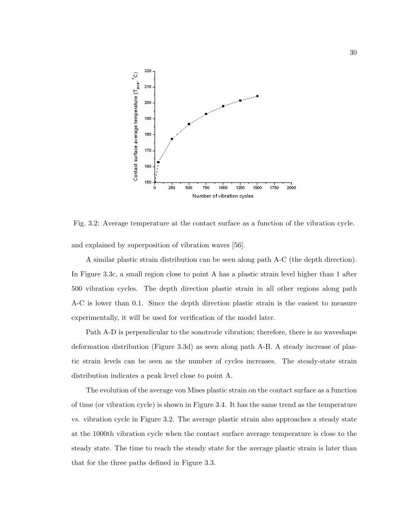
3.2 Average temperature at the contact surface as a function of the vibration cycle. 30

3.3 Distribution of plastic strain as a function of location and vibration cycle. . 31

3.4 Average plastic strain at the contact surface as a function of vibration cycle. 32

3.5 Schematic of changing of substrate’s height. . . . . . . . . . . . . . . . . . . 33

3.6 3-D coupled-field model for validation (a) and distribution of Z-directionalplastic strain (b). . . . . . . . . . . . . . . . . . . . . . . . . . . . . . . . . . 33

3.7 Comparison of experimental measurements and simulation result for the av-erage Z-direction compressive plastic strain. . . . . . . . . . . . . . . . . . . 34

3.8 Definition of paths A-B and C-D. . . . . . . . . . . . . . . . . . . . . . . . . 36

3.9 Compressive normal stress distributions and evolution along path A-B. . . . 36

3.10 Compressive normal stress distributions and evolution along path C-D. . . . 37

3.11 Slide distance distributions and evolution along path A-B. . . . . . . . . . . 38

3.12 Slide distance distributions and evolution along path C-D. . . . . . . . . . . 38

3.13 Shear stress distributions and evolution along path A-B. . . . . . . . . . . . 39

3.14 Shear stress distributions and evolution along path C-D. . . . . . . . . . . . 39

3.15 The 3-D temperature distribution at the 50th vibration cycle (Unit: ◦C). . 40

3.16 Evolution of the top-down-view temperature distribution at : (a) the 10thvibration cycle, (b) the 20th vibration cycle, (c) the 30th vibration cycle, and(d) the 50th vibration cycle (Unit: ◦C). . . . . . . . . . . . . . . . . . . . . 41

3.17 Temperature distributions and evolution along path A-B. . . . . . . . . . . 43

3.18 Temperature distributions and evolution along path C-D. . . . . . . . . . . 43

3.19 3-D von Mises plastic strain distribution at the 50th vibration cycle. . . . . 44

3.20 Evolution of the top-down-view von Mises plastic strain distribution at: (a)the 1st vibration cycle, (b) the 3rd vibration cycle, (c) the 10th vibrationcycle, and (d) the 50th vibration cycle. . . . . . . . . . . . . . . . . . . . . . 45

3.21 Von Mises plastic strain distributions and evolution along path A-B. . . . . 47

xi

3.22 Von Mises plastic strain distributions and evolution along path C-D. . . . . 47

3.23 Average compressive stress on the contact surface vs. vibration cycle. . . . 49

3.24 Average shear stress on the contact surface vs. vibration cycle. . . . . . . . 50

3.25 Average slide distance on the contact surface vs. vibration cycle. . . . . . . 50

3.26 Average heat generation rate by friction on the contact surface vs. vibrationcycle. . . . . . . . . . . . . . . . . . . . . . . . . . . . . . . . . . . . . . . . . 51

3.27 Average heat generation rate by plastic deformation on the contact surfacevs. vibration cycle. . . . . . . . . . . . . . . . . . . . . . . . . . . . . . . . . 51

3.28 Average equivalent heat generation rate on the contact surface vs. vibrationcycle. . . . . . . . . . . . . . . . . . . . . . . . . . . . . . . . . . . . . . . . . 52

3.29 Average temperature on the contact surface vs. vibration cycle. . . . . . . . 52

3.30 Average von Mises plastic strain on the contact surface vs. vibration cycle. 53

3.31 Typical features of fractured surfaces: (a) 87.4% bonded, and (b) 76.4%bonded. . . . . . . . . . . . . . . . . . . . . . . . . . . . . . . . . . . . . . . 55

3.32 Distributions of normalized bonded area and von Mises plastic strain alongpath C-D. . . . . . . . . . . . . . . . . . . . . . . . . . . . . . . . . . . . . . 55

3.33 Correlation of von Mises plastic strain and bonded area. . . . . . . . . . . . 56

4.1 2-D dynamic model for ultrasonic consolidation. . . . . . . . . . . . . . . . . 59

4.2 Static distribution of mechanical status for substrate with a height-to-widthratio of 1.0: (a) contact interface friction status, (b) substrate’s horizontaldisplacement (inch), (c) contact interface horizontal displacement (inch), and(d) contact interface frictional stress (psi). . . . . . . . . . . . . . . . . . . . 60

4.3 Static distributions of stresses and displacement as a function of the H/Wratio: (a) friction stress (psi), and (b) horizontal displacement (inch). . . . . 63

4.4 Distribution of contact displacement (inch) at the 750th cycle with a H/Wratio of 0.75 when the sonotrode moves to opposite directions: (a) left direc-tion displacement, and (b) right direction displacement. . . . . . . . . . . . 66

4.5 Displacement amplitude (inch): (a) at the 750th cycle for substrates withdifferent height-to-width ratios, and (b) for substrate with a height-to-widthratio of 0.75 at different cycles. . . . . . . . . . . . . . . . . . . . . . . . . . 67

xii

4.6 Distribution of shear strain for the substrate with a 0.5 height-to-width ratio:(a) 1st cycle (right), (b) 25th cycle (right), (c) 50th cycle (right), (d) 250thcycle (right), (e) 750th cycle (right), and (f) 750th cycle (left). . . . . . . . 68

4.7 Distribution of shear strain at the 750th cycle for substrate with differentheight-to-width ratios (H/W): (a) H/W=0.25, (b) H/W=0.5, (c) H/W=0.75,(d) H/W=1.0, (e) H/W=1.5, and (f) H/W=2.0. . . . . . . . . . . . . . . . 71

4.8 Interface average shear strain vs. height-to-width ratio at the 750th cycle. . 74

4.9 A model for the analysis of wave traveling in the substrate. . . . . . . . . . 75

4.10 Distribution of shear strain for the substrate with a 0.5 height-to-width ratio:(a) sonotrode moves to the right, and (b) sonotrode moves to the left. . . . 77

5.1 Schematic of the push-pin experiment (a), and setup for the push-pin exper-iment on the Gleeble (b). . . . . . . . . . . . . . . . . . . . . . . . . . . . . 82

5.2 Force vs. displacement curves from push-pin experiments on specimens madewith varying UC process parameters: (a) vibration amplitude, (b) normalpressure, and (c) sonotrode’s travel velocity. . . . . . . . . . . . . . . . . . . 83

5.3 Typical tested push-pin specimen. . . . . . . . . . . . . . . . . . . . . . . . 84

5.4 Finite element model of the push-pin specimen (a), and meshed model (b). 86

5.5 Comparison of force vs. displacement curves from the push-pin experimentand from the FE simulation for specimens made using various process pa-rameters: (a) vibration amplitude, (b) normal pressure, and (c) sonotrode’stravel velocity. . . . . . . . . . . . . . . . . . . . . . . . . . . . . . . . . . . 88

5.6 A typical von Mises strain distribution near the corner of the push-pin hole (a)and a typical z-direction (specimen height direction) stress σzz distributionat the same location (Unit : Pa) (b). . . . . . . . . . . . . . . . . . . . . . . 89

5.7 Bond strength evaluated by PEFE varies with process parameters: (a) vi-bration amplitude, (b) normal pressure, and (c) sonotrode’s travel velocity. 91

5.8 Typical feature of fractured surfaces: (a) 91.6% bonded area, and (b) 74.9%bonded area. . . . . . . . . . . . . . . . . . . . . . . . . . . . . . . . . . . . 93

5.9 Bond strength evaluated by bonded area to total area ratio varying withprocess parameters: (a) vibration amplitude, (b) normal pressure, and (c)sonotrode’s travel velocity. . . . . . . . . . . . . . . . . . . . . . . . . . . . . 94

5.10 Bond strength by PEFE vs. percentage of bonded area (a), and bond strengthas a function of the equivalent crack length, with a comparison betweenstrength obtained using PEFE and strength predicted using Equation 5.3 (b). 95

xiii

5.11 2D temperature-time bond strength map after PWHT (Unit: MPa). . . . . 98

5.12 2D temperature-time failure mode map after PWHT. . . . . . . . . . . . . . 98

5.13 Variation of bond strength after pressurized PWHT with pressure. . . . . . 99

5.14 Variation of buildup deformation after pressurized PWHT with pressure. . . 99

5.15 Variation of bond strength after pressurized PWHT with temperature. . . . 100

5.16 Variation of bond strength after pressurized PWHT with time. . . . . . . . 100

1

Chapter 1

Introduction

1.1 Ultrasonic Welding Description

Ultrasonic welding (UW), as a solid-state joining process, uses an ultrasonic energy

source (usually with a frequency of 20 kHz or above) to induce oscillating shears between the

faying surfaces to produce metallurgical bonds between a wide range of metal sheets [1, 2],

thin foils [3], semiconductors [4], plastics [5], glass [6], and ceramics [7]. In contrast to

traditional fusion welding processes, ultrasonic welding has several inherent advantages [3,8]

derived from its solid-state process characteristics, and has been in use as a versatile joining

method in the electronics, automotive, and aerospace industries since the 1950s.

Recent combination of ultrasonic metal seam welding and CNC milling has resulted

in a new additive manufacturing process known as ultrasonic consolidation (UC) (Figure

1.1) [9, 10]. By continuously welding layers of metal foil to previously deposited material,

during which the profile for each layer is created by contour milling, UC is able to build-

up complex, multi-functional 3-D objects. Objects with complex internal features, objects

made up of multiple materials, and objects integrated with wiring, fiber optics, sensors and

instruments can thus be directly fabricated [3,11,12]. Surface contaminants, such as oxides,

are believed to be fractured and displaced, and atomically clean surfaces are brought into

intimate contact under modest pressures. Researchers are still struggling to understand the

complicated interaction of cyclic motion, large deformation, friction-like shear, localized

thermal effect and oxides/contaminants dispersion on the interface.

Most conventional joining processes use some form of liquid-to-solid material phase

transformation to achieve the transition from a feedstock form to a finished component.

This transformation, and the elevated temperatures associated with melting, put practical

limits on the range of materials that can be deposited, prohibits embedding of temperature-

2

Fig. 1.1: Schematic of ultrasonic welding process.

sensitive devices. As a result, ultrasonic welding has several inherent advantages over other

additive manufacturing and solid freeform fabrication processes [3, 8, 12, 13], including: (1)

Temperature-sensitive devices (e.g. electronics, sensors, actuators, etc.) can be embedded

within the structure, as it is built, without thermal damage. (2) Solid state processing

facilitates retention of nonequilibrium microstructures produced during prior processing.

(3) No atmosphere control is required to inhibit molten metal oxide formation. (4) Residual

stresses and the resultant dimensional distortion may be reduced due to the lack of liquid-

solid transformations. (5) Higher deposition rates are achievable at a lower overall energy

consumption. (6) Dissimilar metals can be joined without melting mixing of the materials.

One unique aspect of UW is that highly localized plastic flow around embedded struc-

tures (e.g. ceramic fibers and wire meshes) is possible, resulting in sound physical/mechanical

bonding between the embedded material and the matrix material [12–14]. Although the

exact mechanisms by which this occurs are only just beginning to be investigated, this ca-

pability can be utilized in several ways, including: (1) manufacture of fiber-reinforced metal

matrix composite with structural fibers for localized stiffening, (2) embedding of optical

3

fibers for communication and sensing, (3) embedding of shape memory fibers for actuation,

and (4) embedding of wire meshes for planar or area stiffening.

1.2 Bonding Mechanisms of UW

Although numerous researchers have been studying the bonding mechanisms of ultra-

sonic welding for over 50 years, the process is still arguably the least understood welding

process. Various mechanisms have been proposed for ultrasonic welding including inter-

diffusion, re-crystallization, plastic deformation, work hardening, breaking of contaminant,

generation of heat by friction and plastic deformation, and even melting [15, 16]. Diffusion

has been observed at the interface between copper and aluminum welds for an extended

period of welding time [17, 18]. And it has also been found that diffusion occurs along

grain boundaries rather than in the bulk of the material [19]. Kreye [20] examined the

microstructure at the weld interface with TEM and claimed that the very small grain size

observed in a thin layer could only be explained by melting and solidification. However,

Harthoorn [21] and Heymann [22] concluded that neither diffusion nor re-crystallization

could be responsible for the joint formation of ultrasonic welding after comparing low fre-

quency vibration welding with ultrasonic welding of aluminum and examining the copper

and soft iron ultrasonic welding. A great deal of plastic deformation and metal flow occur

across the interface, and flow lines, evidence of extensive plastic deformation, are visible in

the bond zone [3, 14, 23]. For the ultrasonic welding of aluminum foil, plastic flow occurs

in a narrow interfacial zone about 10-20 microns in width [3]. In this region, new subgrain

structures form across the bond zone. When the relative motion at the beginning of the

welding cycle cleans the surfaces and plastically deforms asperities [24], microwelds – areas

in which the friction exceeds the flow stress level of the material and plastic metal flow

has started – occur immediately between points of contact of the adjacent surfaces, and

spread out until a sufficient weld area is built up [15, 16]. Zhou et al. have investigated

the effects of process parameters on bond formation in thermosonic gold ball bonding on

a copper substrate at ambient temperatures with scanning electron microscopy [25]. They

concluded that a relative motion existed at the bonding interface as microslip at lower pow-

4

ers, transitioning into gross sliding at higher powers. Researchers in a variety of fields have

observed that ultrasonic excitation of metals can produce an apparent reduction in the yield

strength, and enhancement in the plastic flow of metals [26,27].

Due to the difficulties in definitively characterizing the ultrasonic welding process, the

mechanism(s) for bond formation in UW process are still under debate. The challenges

for measurement approach and instrumentation come from the fact that: (1) the contact

surface where the bonding occurs is invisible to observers; (2) the measurement devices

or sensors tend to damage the contact surface and interfere with the bonding process;

(3) ultrasonic bonding is highly localized (a few millimeters), and transient (typically 20

kHz vibration); and (4) the high spatial resolution (micron-scale vibration amplitude) is

required. To overcome those obstacles and to gain insights on the UW process, numerous

researchers have developed analytical [2, 14,28] and numerical models [10,29–36].

1.3 Modeling of UW

During the last decade, ultrasonic welding has become a popular technique for joining

thermoplastic polymers. Many studies were conducted modeling the process. Senchenkov

et al. [37, 38] studied the problem of vibrations and the dissipative heating of a viscoelas-

tic prism by a waveguide. Benatar and Gutowski [39] modeled the ultrasonic welding of

thermoplastics using a five-part model that included mechanics and vibration of the parts,

viscoelastic heating, heat transfer, flow and wetting, and intermolecular diffusion. Roylance

et al. [40] outlined numerical simulation methods useful in understanding and developing

UW for polymers. Verderber [41] implemented algorithms in an explicit FE analysis code

applicable to the unique features of ultrasonic welding analysis. Senchenkov and Zhuk [42]

studied the two-dimensional problem of planar oscillations of plates under cyclic loading.

The model developed was applied to simulation of vibration of sonotrodes for ultrasonic

welding of plastics. A similar study by Mikhailenko and Franovskii [43] proposed a two-

dimensional FE model that linked thermoelectric processes in acoustic systems.

Numerical modeling of ultrasonic welding of metals and alloys began recently, with

the development of emerging new technologies that employ UW in ultrasonic consolidation

5

[3,44,45]. Compared with ultrasonic welding of polymers, ultrasonic welding of metals seems

to be more challenging to model. In metals, vibration and heat have effects on dislocation

dynamics, metallurgical transformations, and associated variations in thermomechanical

properties [46].

Gao and Doumanidis [14,28] analyzed the mechanics of metal ultrasonic welding. They

developed a 2-D, quasi-static/dynamic, elasto-plastic numerical model of the stress/strain

field by FE analysis. In the study by de Vries [2], mechanics-based models were developed,

along with a model for temperature generation and effect on mechanical properties of welded

material. His models were capable of calculating the interface forces that were verified

experimentally. Siddiq and Ghassemieh [35, 36] studied the change in the friction work at

the weld interface by simulating UW of metals based on a phenomenological material model,

which incorporated both surface (friction) and volume (plasticity) “softening” effects. Ding

et al. [33, 34] analyzed deformation and stress distributions in wire and bond pad during

ultrasonic wire bonding using 2-D and 3-D finite element models. A coupled temperature-

displacement FE analysis performed by Huang and Ghassemieh [31] found the oscillation of

stress in the substrate to lag behind the ultrasonic vibration by about 0.1 cycle of ultrasonic

wave. Yadav and Doumanidis [32] performed the FE analysis of two layers of aluminum

foil subjected to certain welding conditions - with surface contact resistance calibrated by

experiments. The results revealed a moderate temperature rise that was believed to be

sufficient for metal bonding via vacancy diffusion.

1.4 Result Summary of Previous UW Research

1.4.1 Vibration

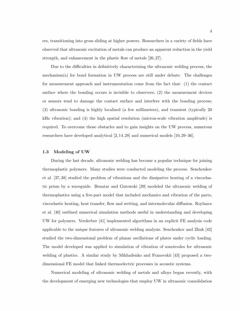
The vibration of the sonotrode with constant pressure produces cyclic sliding at the

bonding interface, along with periodic variation of the elastic/plastic strain/stress state, as

illustrated in Figure 1.2 [28]. The resultant shear stress at the interface is helpful to break

the oxides/contaminants and to generate intimate contact between the faying surfaces.

The overall effect of ultrasonic vibration of the bonding interface can be summarized by

6

Fig. 1.2: Equivalent stress field εeq at three steps of one ultrasonic cycle.

the so-called “acoustic softening” of metals. Based on a phenomenological model, the

stress required to initiate metal plastic deformation decreased significantly with ultrasonic

excitation. The material softening effect has been studied by evaluating the sonotrode

displacement in the height direction, illustrated in Figure 1.3 [31]. It is found that the

sonotrode moves downward continuouly during the whole UW process, under a constant

load on the sonotrode. A similar effect was observed experimentally. This softening effect

becomes more significant if the friction coefficient of the interface is higher.

1.4.2 Friction Work and Temperature

For those areas with the slipping contact condition, the shear stress results in the gen-

eration of friction heat. The friction work is affected by the vibration amplitude, illustrated

in Figure 1.4, but has a non-linear relation with the applied pressure [36]. The roughness of

contact surface decreases under the existence of cyclic shear stress from sonotrode vibration

7

Fig. 1.3: Displacements of the sonotrode versus time along the height direction using differ-ent friction models. The external force applied on the sonotrode is 80N. Friction coefficientequation is defined as: µ = E

p [εxx(t)+ν], where E and ν are the modulus and Poisson ratio,and p is constant pressure.

so as to facilitate the interface ultrasonic bonding.

Due to the heat generation from friction work, the temperature on the bonding interface

increases during UW. The generated heat can dissipate quickly across the entire contact

surface for aluminum alloys. Some simulation results show the maximum temperature to be

located at the foil/sonotrode interface (Figure 1.5), resulted from severe plastic deformation

[36]. These simulation results seem to match the experimental observation of temperature

measurement by high-speed thermal camera [2]. The consequence of temperature rise is to

reduce the stress state of the contact interface by decreasing the material properties, and

the friction coefficient. Thus, the friction work decreases with temperature rise.

1.4.3 Plastic Deformation

A large von Mises plastic strain may result in bonded areas. Plastic deformation is

believed to affect the bond formation in the following ways: (1) it will disperse the surface

oxide layer; (2) it will generate heat to make the atoms more thermally active; (3) it will

deform the crystals and grains on the interfaces and generate a high dislocation density,

which will also provide potential energy for grain boundary migration. Therefore, the plastic

8

Fig. 1.4: Friction work at foil/substrate interface, velocity = 27.8mm/s.

Fig. 1.5: Temperature in the weld specimen (amplitude = 8.4 µm, velocity = 27.8mm/sand pressure = 125MPa).

deformation from the simulation model can be quantitatively correlated with the bonded

area (bond strength) from experiments.

Another quantitative approach for building the relationship between the simulated

and experimental data is to measure the dimension of dynamic recrystallized grains. From

experiments, it is found the crystals may have been dynamically recrystallized into nano-

sized grains during processing (Figure 1.6) [13]. At the beginning of bonding, the plastic

strain is relatively small. The highest plastic strain occurs at the edge of the contact surface.

Subsequently, the plastic deformation in the center of the contact surface exceeds the level

of plastic strain at the edge and becomes the highest. This phenomenon is observed from

the fracture surface (Figure 1.7) [2].

9

Fig. 1.6: Inverse pole figure of an unconsolidated portion of the Ni-Ni interface. Note theextremely fine grains that are present along the defect boundaries.

Fig. 1.7: Fracture interface of Al 6061 parts by UW after peel apart.

1.4.4 Bond Strength

The peeling test has been widely used to measure the bond strength of UW-made

laminated structures by examining the peak load [47]. The bond strength is significantly

influenced by process parameters. The bond strength increases with the vibration amplitude

and preheat temperature, decreases with the sontorode traveling speed, but shows a non-

linear relation with normal pressure [48,49].

Indicators from both experiment and simulation are employed to predict the true bond

strength. Linear weld density (LWD), defined as the length of bonded interface divided by

the total interface length under consideration (expressed in percentage), has a good linear

relation with bond strength (Figure 1.8), but a significant increase of LWD only resulted

10

small increase in the bond strength [47]. Friction work from simulation has also been used

to estimate the bond strength of UW parts [35]. The drawback of friction work as an energy

bond strength indicator is the neglect of contributions of plastic heat and vibration energy.

Fig. 1.8: Correlation of weld strength with LWD of welded Al 6061 specimens.

1.5 Research Plan and Potential Impact

Based on the literature survey and preliminary study of this thesis work, metals under

ultrasonic bonding simultaneously experience the complex and interactive processes of fric-

tion, heat generation, material softening and diffusion under the elevated temperature, and

material flow and hardening. Therefore, a fundamental understanding of this ultrasonic

thermomechanical bonding phenomena requires a systematic approach covering all these

aspects. However, previous experimental studies of UW, based on the post-weld observa-

tions and analysis, resulted in different, and even contradictory conclusions regarding the

bonding mechanisms because of the “black box” approach in the understanding of bond

formation. The reported models of UW focused on either the single mechanical/thermal

behavior, or one-way coupled effect of ultrasonic bond formation. These models are still

unable to fully interpret the physical, thermomechanical bonding phenomena. No direct

relevance of the model was provided for a mechanistic understanding. It is also notable

that none of the reported modeling work provided validation, presumably due to the dif-

ficulties of strain/stress, temperature, and displacement measurements in real-time during

11

ultrasonic welding [23,31].

Therefore, there is no universally-acknowledged theory for bond formation of UW cur-

rently. This work first identified the ultrasonic bonding process as a thermomechanical

coupled problem, and proposed that a bond mechanism study has to be focused on a com-

plete understanding and interpretation of the thermomechanical coupling history at the

bonding interface. This work has developed an integrated set of innovative methods for

this purpose. A 3D numerical model for simulating the UW process has been developed.

A scheme for quantitatively studying the fully thermomechanical coupling effects, espe-

cially the calculation of the effect of plastic deformation, has been designed and realized.

The data of temperature-dependent friction coefficient have been measured. The approach

of quantitative bond strength determination and potential of bond strength improvement

with a pressurized post-weld heat treatment have been proposed. This work has successfully

solved the problem of non-linear multi-physics analysis and the function of plastic defor-

mation work in UW, and has expanded the capabilities of current commercial FE software

packages. With respect to the theoretical contributions to the bonding mechanism of UW,

the fully thermomechanical coupling effect during bond formation has been qualitatively

described, the roles and contributions of in-process thermomechanical variables to the ul-

trasonic bonding have been identified and validated with experiments, and finally a possible

bonding mechanism for ultrasonic metal welding is proposed. In the study of influences of

substrate dimensions on the ultrasonic bonding, the travel, reflection and interference of

ultrasonic waves within the substrate have been found and proved to play a critical role in

ultrasonic bond formation, which may even cause an interface de-bonding problem in the

worst case.

This thesis work has followed the following plan of studies: (1) A series of simula-

tion will be conducted for different process parameters. Then the simulation results will

be analyzed so that the relationship among the process parameters (pressure, amplitude,

traveling speed), in-process variables (contact surface shear stress, sliding distance, heat

generation, temperature and elastic vibration), and the final result (plastic deformation)

12

will be revealed. (2) The push-pin tests will be designed and conducted for each simulation

condition to obtain the bond strength. A detailed analysis of fracture surface will be con-

ducted to find out the local/bulk distribution of the bonded area-ratio and bond strength.

(3) The correlation of plastic deformation and bond strength will be established based on a

detailed and quantitatively study of local/bulk plastic deformation and bond strength data.

(4) The influence of substrate geometry on bond formation will be studied. (5) The bonding

mechanism for ultrasonic metal welding will be proposed. The bond strength will be pre-

dictable if given a set of process parameters. (6) The pressurized post-weld heat treatment

tests will be conducted to explore the potential bond strength improvement method.

Welding process simulation on a thermomechanical fully coupled model provides quan-

titative information on the bonding interface and overcomes the difficulty in data acquisition

in the real manufacturing process, particularly for a process in which the phenomena are

localized, non-equilibrium, and coupled. Bond strength obtained by a specially designed

experiment serves as the strong verification of the simulation work. This thesis work will

have the following deliverables:

1. The complete and accurate temperature-dependent material properties of Aluminum

3003-H18, including the friction coefficient, Young’s modulus, stress-strain curves;

2. A 3D thermomechanical fully coupled finite element model;

3. The systematic quantitative identifications of transient histories, distributions and

interactions of in-process variables, which include normal stress, shear stress, plastic

deformation, heat generation and temperature;

4. A general approach of bond strength determination, and the identifications of bond

strength value for different process parameters;

5. The effects of substrate geometry on ultrasonic bond formation, and the ultrasonic

energy generation and transfer;

6. The comprehensive insights of thermomechanical coupled phenomena and ultrasonic

bonding mechanism;

13

7. The potential of bond strength improvement and the optimum conditions of pressur-

ized post-weld heat treatment.

As a result of this work, a more complete understanding of the physical phenomena

that govern ultrasonic joining has been developed. This will lead to more effective con-

trol of ultrasonic welding operations. As a solid-state process with many inherent benefits

over other joining technologies, ultrasonic welding has the potential to dramatically affect

a number of key industries, including defense, aerospace, automative, and general manu-

facturing. The use of ultrasonic welding to form fiber-reinforced metal matrix composites

from engineering material matrices, to form dissimilar metal thermal management devices

with optimized thermal expansion and conductivity, or to form complex components with

embedded functionality, has the potential to provide design breakthroughs for the electron-

ics, aerospace and transportation industries, among others. This proposal also provides

a general solution strategy concerning the bonding of coupled multi-field and non-melting

process, such as friction-stir welding.

14

Chapter 2

Methodology and Theoretical Background

2.1 Methodology of UW Modeling

2.1.1 Fully Coupled Thermomechanical Model

Based on the above literature review, it is seen that the reported models of metal

UW focused on either the single mechanical/thermal behavior, or one-way coupled effect

of ultrasonic bonding formation. However, the ultrasonic bond formation is believed to be

a complex physical thermomechanical coupled bonding phenomena. This thesis work first

considered the mechanism of ultrasonic bonding as a thermomechanical coupled problem

and tried to numerically interpret this phenomena with a new 3D fully coupled thermome-

chanical non-linear FE model based on ANSYS. Compared with previous numerical models

of UW, this developed model is capable of analyzing the non-linear transient fully coupled

effects of shear stress, friction heat flux, plastic deformation and plastic heat flux simul-

taneously. The heat generation by plastic deformation is first introduced into the bond

mechanism study and UW numerical modeling.

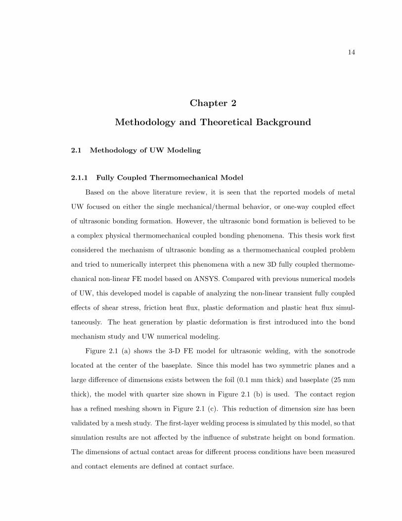
Figure 2.1 (a) shows the 3-D FE model for ultrasonic welding, with the sonotrode

located at the center of the baseplate. Since this model has two symmetric planes and a

large difference of dimensions exists between the foil (0.1 mm thick) and baseplate (25 mm

thick), the model with quarter size shown in Figure 2.1 (b) is used. The contact region

has a refined meshing shown in Figure 2.1 (c). This reduction of dimension size has been

validated by a mesh study. The first-layer welding process is simulated by this model, so that

simulation results are not affected by the influence of substrate height on bond formation.

The dimensions of actual contact areas for different process conditions have been measured

and contact elements are defined at contact surface.

15

Fig. 2.1: The 3-D fully coupled thermomechanical FE model for ultrasonic welding.

16

The multi-physics analysis of commercial FE softwares in particular the GUI is not

able to satisfy the needs of simulating the fully thermomechanical coupled problem of UW.

Their limitations are from two aspects: 1) The multi-physics analysis has to proceed under

the condition of linear analysis; 2) The heat flux from plastic deformation can not be

directly calculated in the current FE software. Therefore, a new customized algorithm is

developed to extend the functions of material non-linear analysis (plastic deformation) and

related thermal effects (heat generation from plastic deformation) to the thermomechanical

multi-physics analysis. The fully coupled thermomechanical analysis algorithm for the above

model has been developed. Definitions of variables and the iteration process for determining

the in-process variable matrices for each ultrasonic vibration cycle are shown in Figure 2.2.

(1) A thermal-structural analysis is conducted first to obtain the temperature field.

Variables from the last step ([εts]j−1, [σts]j−1, and [T]j−1) are input as the initial condi-

tions. Plastic heat [PH]j−1 from the last step is applied as the thermal load. Materials

properties [MP]j−1 and boundary conditions [BC]j are also provided. The [BC]j include

the fixed/symmetric constraints and vibrational motion of the sonotrode. The output pa-

rameters of this coupled thermomechanical analysis are [εts]j , [σts]j , and [T]j , which will

replace the old values from the last step. Based on [T]j , [MP]j−1 is also updated. The fric-

tion heat flux is calculated from the shear stress and slide distance of the contact interface.

The temperature field [T]j results from friction and plastic heat fluxes, as well as the heat

transfer.

(2) A structural analysis is conducted second to obtain the stress and plastic deforma-

tion fields. The variables from the last step ([εs]j−1 and [σs]j−1) are input as the initial

conditions. Temperature [T]j is applied as the thermal load. The outputs of this analysis

are [εs]j and [σs]j , which will replace the values from the last step. The increase of plastic

deformation is used to calculate the plastic heat [PH]j .

During numerical simulation, at each vibration cycle, most of material properties, such

as modulus of elasticity, yield strength and friction coefficient, are temperature sensitive,

so these varying material properties under the temperature of the previous time step must

17

be known and updated before getting the solution of the current cycle.

Fig. 2.2: Thermomechanical coupled analysis diagram for ultrasonic welding process: j isthe jth number of vibration cycle; N is the total number of vibration cycle; [T] is thetemperature matrix; [εts], [σts], and [εs], [σs] are the strain and stress matrixes for thermal-structural and structural analysis, respectively; [MP], [BC] and [PH] are the matrixes formaterial properties, boundary conditions and plastic heat flux.

18

2.1.2 Temperature-dependent Material Properties

Tensile tests have been conducted on the Gleeble 1500D thermomechanical simulator

for measuring the temperature-dependent mechanical properties of aluminum foil (Al 3003-

H18) used in this study. The dimensions of test samples are 22.0×10.1×0.1 mm, and the

tensile load rate is 1.2 mm/min. Specimens were heated to various temperatures and held

for 3 min for thermal equilibrium, and tensile pulled. The results are listed in Table 2.1. It

is seen that the properties of aluminum material are very sensitive to the temperature. At

the preheating temperature (150 ◦C), the mechanical properties decrease to the half or even

less of those at room temperature. The measured yield strength data of aluminum foil are

different, but close to those from the reference. The composition and thermal properties

for Al 3003-H18 are shown in Tables 2.2 and 2.3 [50].

Table 2.1: Temperature-dependent Mechanical Properties of Al 3003-H18

Temp. Modulus of Elasticity Yield Strength Yield Strength∗

(oC) (GPa) (MPa) (MPa)

25 53.2 227.3 18550 28.8 197.3 -100 26.8 131.2 145150 22.7 70.0 -200 16.9 68.3 62250 16.42 32.85 -300 14.5 29 17350 13.26 26.5 -

∗: Data come from Ref. [50].

Table 2.2: Material Components Properties of Al 3003-H18 (%)

Al Cu Fe Mn Si Zn

96.7-99.0 0.050-0.200 ≤0.700 1.00-1.50 ≤0.600 ≤0.100

2.1.3 Friction Coefficient

As a friction-based welding process, there is no doubt that the friction coefficient at

the faying interfaces plays a key role by affecting the stress/strain state and surface heat

19

Table 2.3: Thermal Properties of Al 3003-H18

CTE Specific Heat Capacity Thermal Conductivity(µm/m-oC) (J/g-oC) (W/m-K)

25.1 0.893 155

Fig. 2.3: Experimentally identified history of friction coefficient of Al 1100 foils during oneweld.

generation in UW. It can be said that the ultrasonic bond formation stems from the shear

stress on the interface, which is mainly determined by the friction coefficient, since the

existence of shear stress on the interface generates the friction heat flux, and consequent

plastic deformation and heat flux. Gao and Doumanidis [28] experimentally determined

the friction efficient history of Al 1100 foils during one cycle (Figure 2.3). Siddiq and

Ghassemieh [35,36] numerically described the friction coefficient varying with temperature

and vibration cycle by curve-fitting the published experimental data. Based on Coulomb’s

friction law, the stick-slip contact condition can be identified with the relation of | τfric |

and µ · p. If | τfric |< µ · p, the friction is of the stick-type, and if | τfric |= µ · p, the friction

is of the slip-type.

Regarding the thermomechanical analysis of UW process, the friction coefficient varying

20

with the vibration cycle is believed to be caused by the elevated temperature on the bonding

interface. However, the data of temperature-dependent friction coefficient is still unavail-

able, and the previous UW models ignored the effect of temperature on the friction coeffi-

cient. Therefore, a novel approach for measuring the Al-Al temperature-dependent friction

coefficient has been designed and conducted on the Gleeble 1500D. With this method, the

obtained temperature-dependent friction coefficient can improve the accuracy of the UW

simulation.

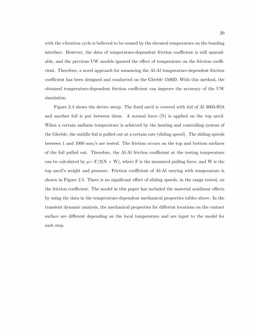
Figure 2.4 shows the device setup. The fixed anvil is covered with foil of Al 3003-H18

and another foil is put between them. A normal force (N) is applied on the top anvil.

When a certain uniform temperature is achieved by the heating and controlling system of

the Gleeble, the middle foil is pulled out at a certain rate (sliding speed). The sliding speeds

between 1 and 1000 mm/s are tested. The friction occurs on the top and bottom surfaces

of the foil pulled out. Therefore, the Al-Al friction coefficient at the testing temperature

can be calculated by µ= F/2(N + W), where F is the measured pulling force, and W is the

top anvil’s weight and pressure. Friction coefficient of Al-Al varying with temperature is

shown in Figure 2.5. There is no significant effect of sliding speeds, in the range tested, on

the friction coefficient. The model in this paper has included the material nonlinear effects

by using the data in the temperature-dependent mechanical properties tables above. In the

transient dynamic analysis, the mechanical properties for different locations on the contact

surface are different depending on the local temperature and are input to the model for

each step.

21

Fig. 2.4: Schematic of Al-Al friction coefficient measurement on Gleeble 1500D.

Fig. 2.5: Al-Al friction coefficient varying with temperature.

22

Fig. 2.6: Mechanical work done during each vibration cycle of UW.

2.1.4 Heat Generation in UW

The ultrasonic mechanical energy, subsequently converted to thermal energy, can be

determined by the local cyclic stress (σ), strain (ε), friction shear (τx), and component slip

(ex) at the interface surface. Heat is generated (a) locally in the control volume, (Qv(x,

y, z)), by inelastic hysteresis and plastic deformation, and (b) at the interface surfaces,

(Qs(x, y)), by friction, during each cycle at the ultrasonic frequency, f , as shown in Figure

2.6 [2, 32,33].

Qv(x, y, z) = f

∮σeq(ε)dεeq (2.1)

Qs(x, y) = f

∮τx(εx)dex = N

∮µσz(εx)dex (2.2)

where σeq and εeq are equivalent stress and strain, and σz is normal compressive stress.

It is first tried to embed the plastic work in the numerical thermomechanical coupled

analysis of UW and quantitatively study the role of plastic work in ultrasonic bond forma-

tion. The above equations for calculating heat generation assume the mechanical state as a

function of location only, not considering time and temperature influences. This thesis pro-

posed a new method of calculating the plastic work, which uses the plastic work rate (W pl),

proportional to the plastic strain rate, to account for the effects of location, temperature

23

and time in UW.

W pl(x, y, z, t, T ) = σj(x, y, z, t, T ) · εplj (x, y, z, t, T ) (2.3)

where j = 1, 2, 3. It is assumed that some of the plastic work converts to heat, while the

rest is stored as energy of crystal defects accompanying plastic deformation. The fraction

of the plastic work (Qpl/W pl) that is converted to thermoplastic heating (Qpl) is 0.33 for

aluminum [51].

2.1.5 Initial and Boundary Conditions

The UC process parameters, including pressure load (1800 N), preheating temperature

(150◦C), vibration amplitude (16 µm), and vibration frequency (20 kHz), are incorporated

in the model as boundary conditions. The pressure load and vibrational displacement are

applied to the interface of foil and baseplate. A triangle wave is used to approximate the

sinusoidal waveform of the ultrasonic vibration. The measured contact area under 1800 N is

4.7 mm along the direction of the sonotrode’s moving, and the sonotrodes speed in the UC

process is set at 28 mm/s. For a given point underneath the sonotrode, the maximum time

of contact is approximately 0.16 s, or about 3000 cycles of vibration. Therefore, we assume

a stationary sonotrode in the model, and the maximum number of cycles to be modeled

is 3000. A fixed boundary condition for displacement is applied to the baseplate’s bottom

surface and all corners except the surface contacting the sonotrode. Symmetrical boundary

conditions are used on two symmetrical planes. A uniform initial preheating temperature

is applied to the parts around the bonding surface, including the sonotrode, baseplate, and

foil. No convective heat loss from baseplate and sonotrode to air is assumed because the

UC device is in an enclosed space in which there is no significant air flow. The radiation

heat loss is also ignored due to the low temperature range.

24

2.2 Theoretical Background

2.2.1 Governing Equations of Thermomechanical Processes

In the modeling of UW processes, the governing dynamic equation of displacement (u)

for a linear structure [52] is:

[M ] {u}+ [C] {u}+ [K]{u} = {L} (2.4)

where [M ] is the structural mass matrix, [C] is the structural damping matrix, [K] is the

structural stiffness matrix, u is the nodal acceleration vector, u is the nodal velocity vector,

{u} is the nodal displacement vector, and {L} is the applied load vector.

The basic constitutive equations between stress (σ) and strain (ε) are as follows:

{σ} = [D]{εel} (2.5)

{εel} = {ε} − {εpl} − {εth} (2.6)

where {σ} is the stress vector, [D] is the elastic stiffness matrix which is a function of

temperature, {εel} is the elastic strain vector, {ε} is the total strain vector, {εpl} is the

plastic strain vector, and {εth} is the thermal strain vector.

Conductive heat transfer can be considered using the following governing equation:

ρc

(∂T

∂t+ (~v · ∇)T

)= q +∇ · (( ~K · ∇)T ) (2.7)

where ρ is the density, c is the specific heat, T is the temperature, t is the time, ~v is the

velocity vector for mass transport of heat, q is the heat generation rate per unit volume, ~K

is the conductivity vector, and ∇ = ∂∂x + ∂

∂y + ∂∂z .

Ultrasonic welding has been identified as a two-way coupled thermomechanical prob-

lem for: (1) the thermal field affects the mechanical field, because most of the material

properties, such as modulus of elasticity, yield strength, and friction coefficient, are tem-

25

perature sensitive; and (2) the mechanical field (friction and plastic deformation) generates

heat, which affects the thermal field. Therefore, modeling of the UW process demands a

coupled-field analysis method. Because closed-form solutions for coupled-field equations are

difficult to obtain, structural and thermal fields are generally treated separately in analytical

modeling of UW [2,14,28].

Recently, commercial FE packages have expanded their capabilities in solving complex

multi-physics problems; many researchers found it convenient to study involved processes

that are not solvable analytically. In the thermomechanical coupled analysis, the FE ma-

trix equation for mechanical and thermal fields, coupled by the thermoelastic constitutive

equations, is as follows [52]:

[M ] [0]

[0] [0]

{ u }{ T }

+

[C] [0]

[Ctu] [Ct]

{ u }{ T }

+

[K] [Kut]

[0] [Kt]

{ u }{ T }

=

{ L }{ Q }

(2.8)

where [M ] is the element mass matrix, [C] is the element structural damping matrix, [K]

is the element stiffness matrix, {u} is the displacement vector, {F} is the sum of the

element nodal force, [Ct] is the element specific heat matrix, [Kt] is the element diffusion

conductivity matrix, {T} is the temperature vector, {Q} is the sum of the element heat

generation load and element convection surface heat flow vectors, and [Kut] is the element

thermoelastic stiffness matrix ([Kut] = −∫vol[B]T {β}{∇{N}T }d{vol}), where [B] is the

strain-displacement matrix, and [Ctu] is the element thermoelastic damping matrix ([Ctu] =

−To[Kut]T , and To is the absolute reference temperature).

26

2.2.2 Material Behavior in UW

Yield Rule and Plastic Deformation

The von Mises yield criterion has been widely applied in plastic analysis [29, 32]. If

the von Mises equivalent stress is less than the material yield strength at temperature, the

stress state is elastic and no plastic strain is computed. If the stress exceeds the material

yield strength, the plastic strain εpl is calculated by

{dεpl

}= λ

{∂F

∂σ

}(2.9)

where λ determines the amount of plastic straining, and F (yield function) is given by

F =| σ − α | −(σ0 +R) = 0 (2.10)

where σ is stress tensor, α is the back stress tensor due to kinematic hardening, R is the

isotropic hardening term and σ0 is the initial yield stress.

Thermomechanical Hardening Rules

The nonlinear isotropic hardening rule was presented by Lemaitre and Chaboche [53]

and Huber and Tsakmakis [54]. The isotropic hardening (R), which describes the expansion

of the yield surface, is defined as an exponential function of accumulated plastic strain.

R = A(1− e−bεpl) (2.11)

where εpl is the equivalent plastic strain, while A and b are material parameters to be

identified. A is the maximum change in the size of the yield surface, and b is the rate at

which the size of the yield surface changes with changing plastic strains.

A nonlinear kinematic hardening rule proposed by Armstrong and Frederick [55] has

been used to capture nonlinear hardening behavior and the smooth transition from elastic

27

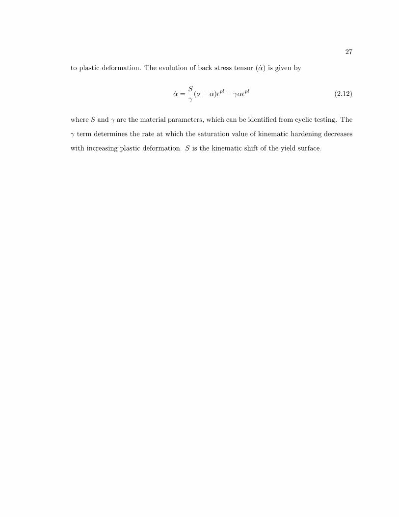
to plastic deformation. The evolution of back stress tensor (α) is given by

α =S

γ(σ − α)εpl − γαεpl (2.12)

where S and γ are the material parameters, which can be identified from cyclic testing. The

γ term determines the rate at which the saturation value of kinematic hardening decreases

with increasing plastic deformation. S is the kinematic shift of the yield surface.

28

Chapter 3

Discussions of Simulation Results and Bonding Mechanism

3.1 Thermomechanical Simulation Results with Friction Heat Generation Only

3.1.1 Effect of Friction on Temperature

Figure 3.1 shows the coordinate plane projections of temperature distribution on the

contact surface (bond interface) at the 1500th vibration cycle. With friction heat, a uni-

form peak temperature state exists on the contact surface, and the temperature decreases

away from the contact surface into the substrate. The temperature distribution shows a

cylindrical symmetry about the center of the contact surface. The average temperature due

to friction at the contact surface increases rapidly with the number of vibration cycles in

the initial period of bonding. As the welding time is longer (higher number of cycles), the

temperature rise slows down, and seems to approach a steady state, as seen in Figure 3.2.

The increase of interface temperature is influenced by qfriction - qloss, where qfriction is the

friction heat generation rate, and qloss = k4T is the heat dissipation rate by conduction.

At the beginning of UW bonding, the rate of friction heat generation is much higher than

that of heat loss, because initially the temperature difference (4T) is low. As the tempera-

ture becomes higher due to friction heating, two competing factors become significant: On

the one hand, the decrease of Young’s modulus (Table 2.1) and friction coefficient (Figure

2.5) will slow down the friction heat generation; on the other hand, the greater temperature

difference enhances faster heat dissipation. Therefore, the temperature increase slows down.

A balance between qfriction and qloss can be achieved eventually, giving rise to qfriction -

qloss = 0, i.e., a thermal steady state. Physically, if the heat loss is faster than the fric-

tion heat generation and the interface temperature decreases, the higher values of Young’s

modulus and friction coefficient at the lower temperature will automatically increase the

29

Fig. 3.1: Distribution of temperature at the 1500th vibration cycle: (a)front view, (b) topview, and (c) side view.

qfriction until a new dynamic heat balance is achieved.

3.1.2 Effect of Friction on Plastic Deformation

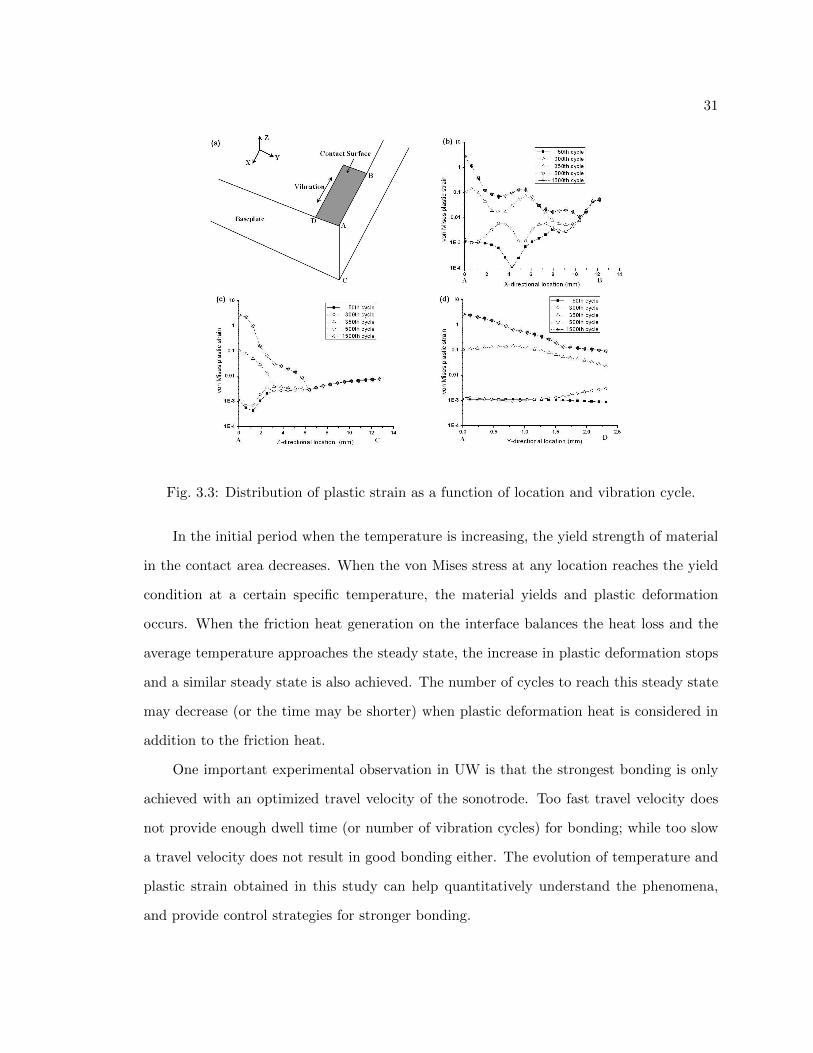
Three paths (A-B, A-C, and A-D) have been selected to show the three-dimensional

distributions of von Mises strain around the contact surface (Figure 3.3a) where the bonding

process happens. Figure 3.3b shows the von Mises strain distributions along path A-B (the

vibration direction) as a function of the number of vibration cycles. At the beginning of

bonding (50th cycle), the plastic strain is relatively small. The highest plastic strain occurs

at the edge of the contact surface near point B. By the 350th cycle, the plastic strain in

the center of the contact surface exceeds the level of plastic strain at the edge. After the

500th vibration cycle, the value and distribution of plastic deformation reach a steady state,

when there is no change in von Mises strain with further increase of the vibration cycle.

The maximum plastic strain is located at point A, the center of the contact surface. A

wavy-shaped plastic strain distribution caused by the cyclic vibration is apparent. The

reason for such a characteristic wave shape distribution of deformation has been studied

30

Fig. 3.2: Average temperature at the contact surface as a function of the vibration cycle.

and explained by superposition of vibration waves [56].

A similar plastic strain distribution can be seen along path A-C (the depth direction).

In Figure 3.3c, a small region close to point A has a plastic strain level higher than 1 after

500 vibration cycles. The depth direction plastic strain in all other regions along path

A-C is lower than 0.1. Since the depth direction plastic strain is the easiest to measure

experimentally, it will be used for verification of the model later.

Path A-D is perpendicular to the sonotrode vibration; therefore, there is no waveshape

deformation distribution (Figure 3.3d) as seen along path A-B. A steady increase of plas-

tic strain levels can be seen as the number of cycles increases. The steady-state strain

distribution indicates a peak level close to point A.

The evolution of the average von Mises plastic strain on the contact surface as a function

of time (or vibration cycle) is shown in Figure 3.4. It has the same trend as the temperature

vs. vibration cycle in Figure 3.2. The average plastic strain also approaches a steady state

at the 1000th vibration cycle when the contact surface average temperature is close to the

steady state. The time to reach the steady state for the average plastic strain is later than

that for the three paths defined in Figure 3.3.

31

Fig. 3.3: Distribution of plastic strain as a function of location and vibration cycle.

In the initial period when the temperature is increasing, the yield strength of material

in the contact area decreases. When the von Mises stress at any location reaches the yield

condition at a certain specific temperature, the material yields and plastic deformation

occurs. When the friction heat generation on the interface balances the heat loss and the

average temperature approaches the steady state, the increase in plastic deformation stops

and a similar steady state is also achieved. The number of cycles to reach this steady state

may decrease (or the time may be shorter) when plastic deformation heat is considered in

addition to the friction heat.

One important experimental observation in UW is that the strongest bonding is only

achieved with an optimized travel velocity of the sonotrode. Too fast travel velocity does

not provide enough dwell time (or number of vibration cycles) for bonding; while too slow

a travel velocity does not result in good bonding either. The evolution of temperature and

plastic strain obtained in this study can help quantitatively understand the phenomena,

and provide control strategies for stronger bonding.

32

Fig. 3.4: Average plastic strain at the contact surface as a function of vibration cycle.

3.1.3 FEM Model Validation

Definition of Z-directional Compressive Equivalent Plastic Strain in Experiment

An experimental validation of the finite element results shown in Figure 3.3c was con-

ducted. In UW, the height of deposit is smaller than the sum of the foil layers’ original

thickness, and the relative ratio changes with the number of layers. Figure 3.5 shows the dif-

ference in substrate height before bonding (a) and after bonding (b). Thus, the Z-directional

compressive equivalent plastic strain can be defined as follows:

εplz,eq =(Ha −Hb)

Hb(3.1)

Samples of various numbers of layers are made on the UW machine with the same

process parameters used in the simulations. The sample heights after UW bonding are

measured with a precision height gauge with a 0.001-mm resolution. The substrate’s height

before bonding is calculated by 0.1 mm (foil thickness) × 8 (layers number). Thus, the

Z-directional compressive equivalent plastic strain from the experiment can be calculated

by Equation 3.1.

33

Fig. 3.5: Schematic of changing of substrate’s height.

Fig. 3.6: 3-D coupled-field model for validation (a) and distribution of Z-directional plasticstrain (b).

Definition of Z-directional Compressive Equivalent Plastic Strain in Simulation

For the purpose of finite element model validation, a new finite element model is de-

veloped to incorporate a rectangular substrate 12.2 mm long and 5.0 mm wide (Figure

3.6a). The same simulation strategy is applied to the new simulation with various buildup

layers. A cut section plane parallel to the vibration direction and located at the center of

the substrate is chosen for extracting the Z-directional plastic strain. Figure 3.6b shows

the distribution of Z-directional plastic strain in the cut section for the eight layers of the

substrate. The average value is calculated and defined as the Z-directional compressive

equivalent plastic strain in simulation.

34

Fig. 3.7: Comparison of experimental measurements and simulation result for the averageZ-direction compressive plastic strain.

Comparison

Figure 3.7 shows the comparison of Z-directional compressive equivalent plastic strain

between experiment measurement and finite element simulation. It can be seen that the

finite element model in this paper is able to correctly predict the trend and magnitude of

the experimental data. The error may be very likely due to the omission of contribution

of plastic heat flux to plastic strain. Another error source is the use of solid substrate in

the validation model instead of the true substrate that actually has a layered structure

and different mechanical properties. When the temperature increases, the tendency for

microstructure change, such as recovery, which is not included in the model, may also

contribute to the error.

35

3.2 Thermomechanical Simulation Results with Both Friction and Plastic De-

formation Heat Generation

3.2.1 Distributions and Evolution of In-process Variables on the Contact Sur-

face

Compressive Normal Stress

To help visualize the stress and strain distributions at the contact interface, paths A-B

and C-D are defined in Figure 3.8, with path C-D along the edge of the contact area, and

path A-B along the centerline underneath the sonotrode. The distributions and evolution

of compressive normal stress (σz) have been extracted and shown in Figures 3.9 and 3.10

along paths A-B and C-D. The distributions of the stress are not uniform, but rather exhibit

a wave feature. As the vibration cycle increases, the compressive normal stress fluctuates

around 180MPa along path A-B, and 140MPa along path C-D. Under the clamping force,

path A-B has the maximum Z-directional displacement, while path C-D has the minimum

displacement. The σz for paths parallel to and in-between A-B and C-D is in the range

between 180MPa and 140MPa.

The significance of σz and its variation is, that combined with the friction coefficient,

it determines the friction stress on the contact surface based on Coulomb’s law of friction.

However, to determine the frictional heat, the shear stress and slide distance are required.

Slide Distance

Along the sonotrode vibration direction, the relative slide movement at the interface

is the result of a superposition of sinusoidal vibration of the sonotrode and vibration of

the baseplate. This relative motion of the contact interface for each vibration cycle can be

defined as the slide distance Lslide = Lst−Lbp, where Lst is the sonotrode moving distance

(Lst = 32µm when the sonotrode makes a peak-to-peak movement with a 16 µm amplitude),

and Lbp is the moving distance of the baseplate during the same period. Depending on the

magnitude and direction of the baseplate movement, Lslide can be greater or smaller than

36

Fig. 3.8: Definition of paths A-B and C-D.

Fig. 3.9: Compressive normal stress distributions and evolution along path A-B.

Lst = 32µm.

The distributions and evolution of the relative slide distance along paths A-B and C-D

on the contact surface are plotted in Figures 3.11 and 3.12. Initially, the slide distance is

37

Fig. 3.10: Compressive normal stress distributions and evolution along path C-D.

smaller than the 32 µm sonotrode distance. As the number of vibration cycles increases,

the slide distance increases. The region close to edge B-D of the contact area has a slide

distance higher than 32 µm. This means the baseplate is vibrating in the opposite direction

against the sonotrode in that region. The same region also experiences the greatest increase

in the slide distance as the number of cycles increases. As can be predicted, the B-D region

will have the greatest frictional heat generation.

Shear Stress

The distributions of shear stress (τxy) at the contact interface show dramatic undu-

lations. A shear stress peak exists at the center of the contact interface (near point A)

on path A-B (Figure 3.13). A shear stress peak exists at the edge of the contact interface

(near point D) on path C-D (Figure 3.14). The average shear stress on path C-D is greater

than that on path A-B. On path C-D, it is also notable that the shear stress undergoes a

greater increase as a function of vibration cycle. The undulations of shear stress at various

locations will produce a similar distribution pattern for friction heat. That effect is clearly

seen in the temperature distributions.

38

Fig. 3.11: Slide distance distributions and evolution along path A-B.

Fig. 3.12: Slide distance distributions and evolution along path C-D.

Temperature

Temperature distribution in the baseplate is shown in Figure 3.15. The peak temper-

ature is located near the edges of the contact interface, and the temperature distribution

in the depth direction is shallow, indicating the highly localized thermal phenomena in ul-

39

Fig. 3.13: Shear stress distributions and evolution along path A-B.

Fig. 3.14: Shear stress distributions and evolution along path C-D.

trasonic bonding. The evolution of the transient temperature field is shown in Figure 3.16

in the top-down view. The distributions and evolution of temperature along paths A-B

and C-D have been plotted in Figures 3.17 and 3.18. The high temperature zone is limited

to a small volume corresponding to the contact surface. This high temperature zone may

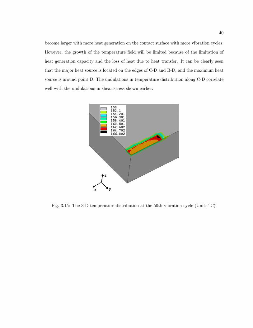
40

become larger with more heat generation on the contact surface with more vibration cycles.

However, the growth of the temperature field will be limited because of the limitation of

heat generation capacity and the loss of heat due to heat transfer. It can be clearly seen

that the major heat source is located on the edges of C-D and B-D, and the maximum heat

source is around point D. The undulations in temperature distribution along C-D correlate

well with the undulations in shear stress shown earlier.

Fig. 3.15: The 3-D temperature distribution at the 50th vibration cycle (Unit: ◦C).

41

Fig. 3.16: Evolution of the top-down-view temperature distribution at : (a) the 10th vi-bration cycle, (b) the 20th vibration cycle, (c) the 30th vibration cycle, and (d) the 50thvibration cycle (Unit: ◦C).

42

Fig. 3.16 continued.

43

Fig. 3.17: Temperature distributions and evolution along path A-B.

Fig. 3.18: Temperature distributions and evolution along path C-D.

44

Plastic Deformation

Figure 3.19 shows the 3-D von Mises plastic strain distribution in the baseplate at the

50th vibration cycle, and its evolution (top-down view) is shown in Figure 3.20. The dis-

tributions and evolution of von Mises plastic stain along the paths A-B and C-D have been

plotted in Figures 3.21 and 3.22. The plastic deformation volume is also limited around the

edges of the contact surface, where the conditions of high stresses and heat generation rate

coexist. It is also found that the plastic deformation area extends toward to the center of the

contact surface with more vibration cycles. It can be predicted that the plastic deformation

will cover the entire contact surface when more plastic deformation is generated with the

sonotrode’s vibration. A higher degree of plastic deformation has been found on path C-D

than path A-B, and on edge B-D than edge C-D. After the 20th vibration cycle, the plastic

deformation stops increasing, indicating a plastic saturation. A fluctuation in distribution of

plastic deformation is also found to correlate with the shear stress distribution (Figure 3.22).

Fig. 3.19: 3-D von Mises plastic strain distribution at the 50th vibration cycle.

45

Fig. 3.20: Evolution of the top-down-view von Mises plastic strain distribution at: (a) the1st vibration cycle, (b) the 3rd vibration cycle, (c) the 10th vibration cycle, and (d) the50th vibration cycle.

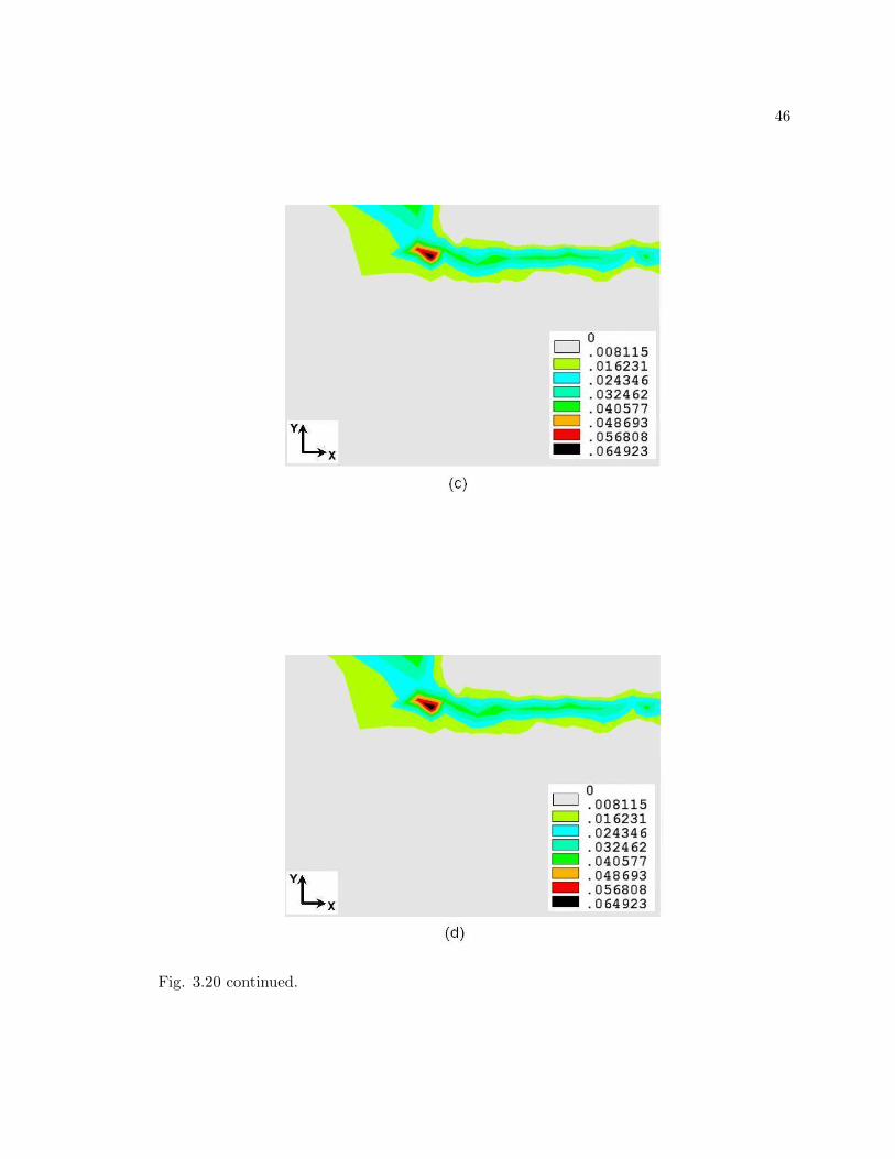
46

Fig. 3.20 continued.

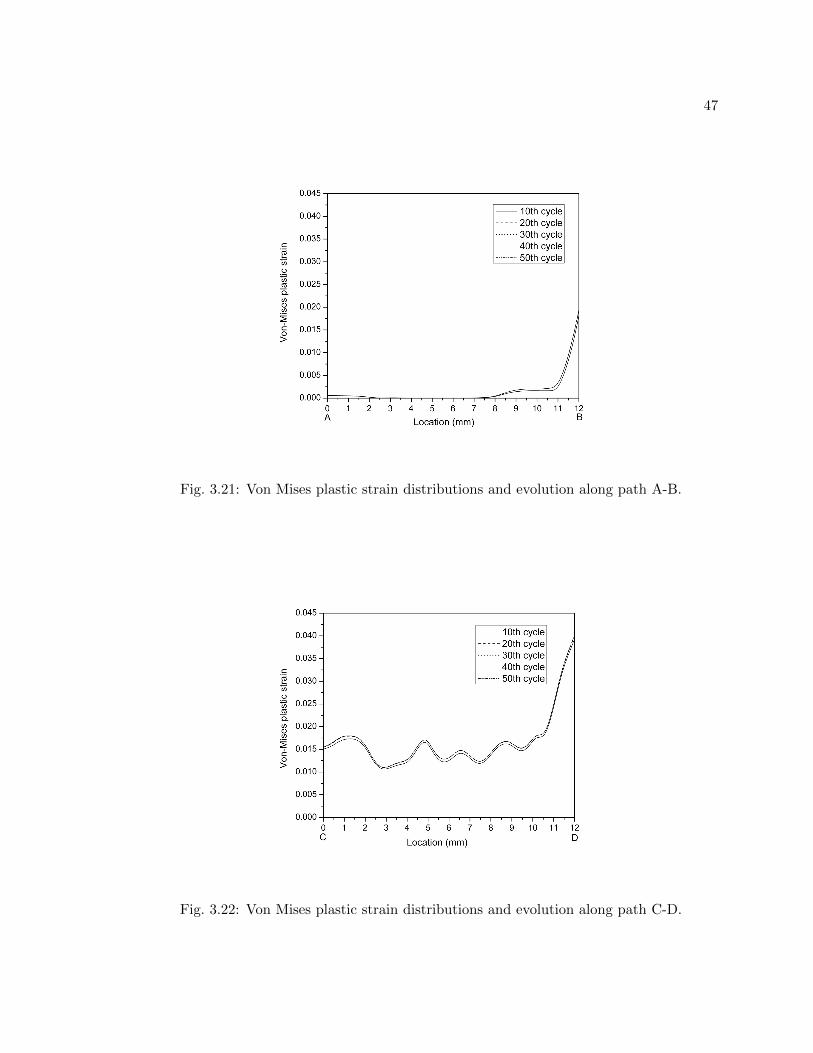
47

Fig. 3.21: Von Mises plastic strain distributions and evolution along path A-B.

Fig. 3.22: Von Mises plastic strain distributions and evolution along path C-D.

48

3.2.2 Evolution of Average In-process Variables in the Bond Zone

To help understand the mechanism of ultrasonic bond formation and to study the

interactions between the thermal and structure fields, the average in-process variables on

the contact surface have been calculated. The surface heat density generation rate by

friction is calculated by τxyLslide/tp, where τxy is shear stress, and tp is the period of

vibration. The volume heat density generation rate by plastic deformation is calculated by

Σσj · ∆εpj/tp, where σj is the principal stresses, ∆εpj is the change in the principal plastic

strains, and j can be 1, 2 or 3. The equivalent volume heat density generation rate can be

obtained by Cρ∆T/tp, where C is specific heat, ρ is the density, and ∆T is the change in

temperature. The net heat accumulation on the contact surface is the total heat generation

subtracted by heat dissipation. Table 3.1 summarizes the average in-process variables in

different periods. The first 50 vibration cycles of ultrasonic welding have been divided into

three periods according to Figure 3.30.

(1) 1st - 10th vibration cycle: When the sonotrode starts to vibrate, a high stress state

(Figures 3.23 and 3.24) is generated because of the high material stiffness at a lower tem-

perature. Therefore, a large plastic deformation increase rate (Figure 3.30) with a high heat

generation rate (Figures 3.26-3.28) is caused by the high stress state. In ultrasonic welding,

two stress components, the normal stress σz and shear stress τxy, are more important than

others. It is the normal stress σz that builds up a high stress state and yields the material,

which contributes to plastic heating (Figure 3.23). The shear stress τxy mainly contributes

to the generation of frictional heat. This observation can be verified by comparing the

variations of frictional heat and that of shear stress τxy (Figures 3.24 and 3.26). Toward the

end of this period, a large temperature increase rate (Figure 3.29) decreases the material

properties rapidly. Consequently, the stresses and heat generation rates reduce fast (Figures

3.23, 3.24, and 3.26-3.28).

(2) 11th - 20th vibration cycle: This period is characterized by a lower heat generation

rate than the previous period (Figures 3.26-3.28). The lower rate of temperature increase

(Figure 3.29) slows down the rate of increase for the normal and shear stresses (Figures 3.23

49

and 3.24). Therefore, although the plastic deformation keeps increasing, its rate of increase

is lower (Figure 3.30).

(3) 21st - 50th vibration cycle: The temperature continues to increase (Figure 3.29),

indicating a positive heat accumulation at the bond interface - the heat generation on the

contact surface is greater than the heat dissipation, although the equivalent heat generation

rate decreases during this period (Figure 3.28). Therefore, the normal stress σz keeps

decreasing (Figure 3.23) because of the decreased material properties. Toward the end

of this period, the plastic deformation (Figure 3.30) has stopped increasing, arriving at a

saturation state.

Fig. 3.23: Average compressive stress on the contact surface vs. vibration cycle.

50

Fig. 3.24: Average shear stress on the contact surface vs. vibration cycle.

Fig. 3.25: Average slide distance on the contact surface vs. vibration cycle.

51

Fig. 3.26: Average heat generation rate by friction on the contact surface vs. vibrationcycle.

Fig. 3.27: Average heat generation rate by plastic deformation on the contact surface vs.vibration cycle.

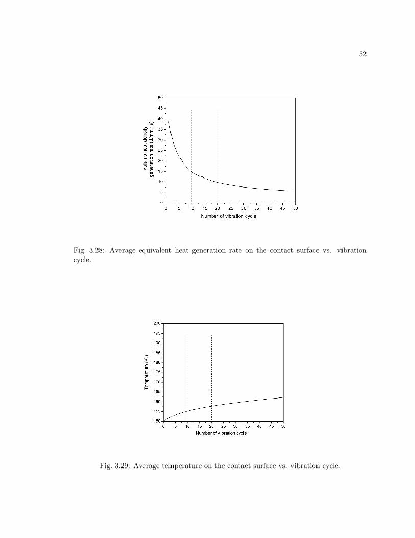
52

Fig. 3.28: Average equivalent heat generation rate on the contact surface vs. vibrationcycle.

Fig. 3.29: Average temperature on the contact surface vs. vibration cycle.

53

Fig. 3.30: Average von Mises plastic strain on the contact surface vs. vibration cycle.

Table 3.1: Evolution of Average In-process Variables on the Contact Surface

In-process variables 1st - 10th cycle 11th - 20th cycle 21st - 50th cycle

Normal stress 182.63 180.41 176.87−σz, (MPa)

Shear stress 5.49 2.43 3.13−τxy, (MPa)

Slide distance 28.50 31.90 31.60Lslide, (µm)

Friction heat generation rate 7.24 3.14 3.94∆Hf/∆t · area, (J/mm2·s)Plastic heat generation rate 1.37 0.03 0.02∆Hp/∆t · vol, J/mm3·s)Net heat accumulation rate 23.21 11.66 7.19∆Ht/∆t · vol, (J/mm3·s)Temperature 153.72 156.32 160.22T, (oC)Changing rate of temperature 1.20e4 4.80e3 3.00e3∆T/∆t, (oC/s)

Plastic deformation 2.32e-3 3.32e-3 3.55e-3(εpvon)Changing rate of plastic deformation 5.52 1.00 6.66e-3∆εpvon/∆t, (1/s)

54

3.2.3 Correlation of Simulation and Experimental Results

It is difficult to validate the numerical models of ultrasonic welding directly because

of the difficulties of experimental measurement due to process characteristics of ultrason-

ic welding. The contact surface where the bonding occurs is invisible to observers, and

measurement devices or sensors tend to damage the contact surface and interfere with the

bonding process. Thermal mechanical processes that are highly localized (a few millimeter-

s), transient (under 20KHz vibration), and require high spatial resolution (the amplitude

of vibration is 16 µm), pose challenges for measurement instrumentation.

However, aluminum foils bonded under different process parameters have been tested

and the typical fractured surfaces are shown in Figure 3.31. The distribution of areas that

are not bonded correlates with the distributions of shear stress and temperature as predicted

by the simulation. The bonded area can be used to evaluate the bond strength.

A rectangular region along path C-D is selected and divided into 16 areas with the

same dimensions. The bonded areas for these divisions have been measured and plotted

in Figure 3.32. von Mises plastic strain has been selected among the in-process variables

from simulation results, because it is a variable that includes the accumulated effect of

both thermal and mechanical processes at the interface. Based on the simulation results,

average von Mises plastic strains on these same 16 divisions for the 50th vibration cycle

have been extracted and plotted in Figure 3.32. The von Mises plastic strains has the same

trend as the bonded area along the chosen stripes on path C-D. A strong linear correlation

between them is also shown in Figure 3.33. Large von Mises plastic strain will result in

more bonded areas. Therefore, it seems reasonable that von Mises plastic deformation from

the simulation model can be quantitatively correlated with the bonded area (bond strength)

from experiments.

Another positive correlation between the simulation and experimental observations is

that our simulation results are able to provide new insights to, and explanations for, the

relations of the in-process variables and their effects on bond formation.

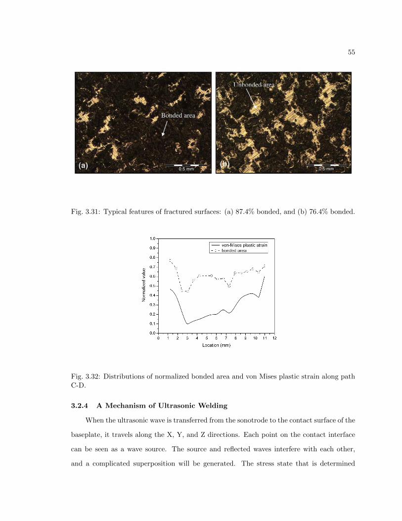
55

Fig. 3.31: Typical features of fractured surfaces: (a) 87.4% bonded, and (b) 76.4% bonded.

Fig. 3.32: Distributions of normalized bonded area and von Mises plastic strain along pathC-D.

3.2.4 A Mechanism of Ultrasonic Welding

When the ultrasonic wave is transferred from the sonotrode to the contact surface of the

baseplate, it travels along the X, Y, and Z directions. Each point on the contact interface

can be seen as a wave source. The source and reflected waves interfere with each other,

and a complicated superposition will be generated. The stress state that is determined

56

Fig. 3.33: Correlation of von Mises plastic strain and bonded area.

by the normal stress and friction conditions at the contact surface will alter the wave

superposition. However, the characteristic wave-like distributions of in-process variables

clearly are the result of wave superposition and vibration modes. A quantitative treatment

of such dynamic effects is given elsewhere [57]. The fracture surface morphology on the

ultrasonic bonding interface (Figure 5.8) is another indication of the ultrasonic vibration

modes.

It appears that the temperature-dependent material stiffness (E) and yield stress (σy)

have different effects on the in-process variables. The material stiffness will mostly affect

the stress state and frictional heat generation, while the yield stress will mostly affect the

generation of plastic strain and plastic heat. Based on the simulation results, a mechanism

for bond formation in ultrasonic welding of an FCC metal (Al) is proposed as follows. (1)

The normal clamping force and sonotrode vibration generate the shear stress (τxy) and shear

strain. The shear strain displaces the oxide layer on the contact surfaces, to expose clean

metal. (2) Shear stress and strain generate the frictional heat, and the plastic strain gen-

erates plastic heat. (3) A temperature rise will result from the equivalent heat generation

determined by the combined effect of the frictional and plastic heat fluxes, and heat dissi-

pation; (4) The rising temperature increases the plastic strain at the interface by lowering

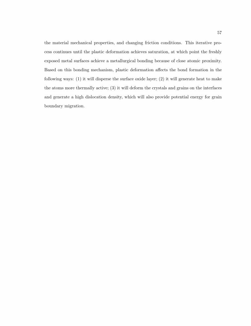
57

the material mechanical properties, and changing friction conditions. This iterative pro-

cess continues until the plastic deformation achieves saturation, at which point the freshly

exposed metal surfaces achieve a metallurgical bonding because of close atomic proximity.

Based on this bonding mechanism, plastic deformation affects the bond formation in the

following ways: (1) it will disperse the surface oxide layer; (2) it will generate heat to make

the atoms more thermally active; (3) it will deform the crystals and grains on the interfaces

and generate a high dislocation density, which will also provide potential energy for grain

boundary migration.

58

Chapter 4

Effect of Substrate Dimensions on Ultrasonic Bonding

A previous study shows that there is a maximum height-to-width ratio of free standing

structures that can be built using ultrasonic consolidation. If the height-to-width ratio is

higher than 1:1, no ultrasonic bonding can be achieved [58]. The objective of this work is

to analyze the UW process by studying the bonding interface and the substrate, and to

show how the ultrasound waves traverse in the substrate and its effect on the interface.

Another objective is to develop the mechanics for ultrasonic consolidation that can explain

the experimental results and point to the direction for ways for new development. An

FEM model is set-up and the distributions of strain/stress in the substrate, and friction

stress/displacement on the interface are analyzed. The FE simulation model has been

validated by an ultrasound wave model.

4.1 A Dynamic Model for Ultrasonic Consolidation

Previous research on ultrasonic bonding has focused on the interface area where the

bonding occurs [23, 59]. However, we found that wave interference within the substrate

has a significant effect on joint formation. Therefore, a dynamic FEM model is developed

to include the sonotrode and the entire substrate for a fundamental study of the time-

dependent mechanical behavior of the substrate in ultrasonic consolidation.

Figure 4.1 shows the 2-D dynamic model involving the sonotrode that is pressed to

contact with and vibrates against the substrate. The model domain is an analytical plane

that is perpendicular to the welding direction and through the center of the sonotrode.

The chosen model plane satisfies the plane strain condition. The base plate is not included

in the model and its influence is simulated by adding a fixed boundary condition at the

bottom surface of the substrate. The titanium sonotrode surface has been roughened so

59

that it is assumed that there is no slipping between the top surface of the aluminum foil

and the sonotrode during vibration. A very large friction coefficient is assumed between

the top aluminum foil and the titanium sonotrode to simulate the no slipping condition

for the sonotrode. Any relative sliding happens between the bottom surface of the top

foil and the substrate. The substrate is assumed to be homogeneous and isotropic. The

Coulombs friction law, that friction is proportional to normal pressure and independent of

slide velocity, is employed in simulation to determine the contact status (sticking or sliding)

and shear stress at the contact interface. It should also be pointed out that the heating

effect is not considered in this model.

Fig. 4.1: 2-D dynamic model for ultrasonic consolidation.

4.2 Static Analysis

Upon the initial application of the pressure on the substrate, and before the first vibra-

tion cycle is applied, the substrate exhibits a static distribution of stress and strain. For the

substrate with an 1.0 height-to-width ratio, the distribution of mechanical status is shown

in Figure 4.2. The friction status at the contact surface is mostly “sticking,” i.e., there is no

relative motion in the horizontal direction between the sonotrode and the substrate. Near

the two edges, however, there are small areas where “sliding” occurs. Right at the edges,

the status of the interface is “near contact.” In Figure 4.2b, the horizontal displacement

of the substrate shows a typical barreled shape: the mid-height of the substrate flows out

undisturbed, while near the contact interface the frictional force opposes the outward flow

60

of the material. This effect is also seen in Figure 4.2c, in which the horizontal displace-

ment at the contact interface reaches its maximum at the boundary between the “sticking”

and “sliding” areas and decreases to zero at the center and the edges of the contact interface.

Fig. 4.2: Static distribution of mechanical status for substrate with a height-to-width ratioof 1.0: (a) contact interface friction status, (b) substrate’s horizontal displacement (inch),(c) contact interface horizontal displacement (inch), and (d) contact interface frictionalstress (psi).

61

Fig. 4.2 continued.

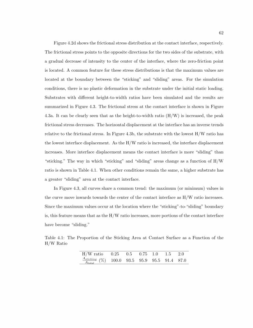
62

Figure 4.2d shows the frictional stress distribution at the contact interface, respectively.

The frictional stress points to the opposite directions for the two sides of the substrate, with

a gradual decrease of intensity to the center of the interface, where the zero-friction point

is located. A common feature for these stress distributions is that the maximum values are

located at the boundary between the “sticking” and “sliding” areas. For the simulation

conditions, there is no plastic deformation in the substrate under the initial static loading.

Substrates with different height-to-width ratios have been simulated and the results are

summarized in Figure 4.3. The frictional stress at the contact interface is shown in Figure

4.3a. It can be clearly seen that as the height-to-width ratio (H/W) is increased, the peak

frictional stress decreases. The horizontal displacement at the interface has an inverse trends

relative to the frictional stress. In Figure 4.3b, the substrate with the lowest H/W ratio has

the lowest interface displacement. As the H/W ratio is increased, the interface displacement

increases. More interface displacement means the contact interface is more “sliding” than

“sticking.” The way in which “sticking” and “sliding” areas change as a function of H/W

ratio is shown in Table 4.1. When other conditions remain the same, a higher substrate has

a greater “sliding” area at the contact interface.

In Figure 4.3, all curves share a common trend: the maximum (or minimum) values in

the curve move inwards towards the center of the contact interface as H/W ratio increases.

Since the maximum values occur at the location where the “sticking”-to-“sliding” boundary

is, this feature means that as the H/W ratio increases, more portions of the contact interface

have become “sliding.”

Table 4.1: The Proportion of the Sticking Area at Contact Surface as a Function of theH/W Ratio

H/W ratio 0.25 0.5 0.75 1.0 1.5 2.0Asticking

Atotal(%) 100.0 93.5 95.9 95.5 91.4 87.0

63

Fig. 4.3: Static distributions of stresses and displacement as a function of the H/W ratio:(a) friction stress (psi), and (b) horizontal displacement (inch).

64

4.3 Dynamic Analysis

When the sonotrode moves in opposite directions, the distributions of the contact

interface displacement retain the same features as the static case. However, the zero-value

point vibrates with the sonotrode (Figure 4.4). The displacement value at each point

of contact exhibits a fluctuating variation with the vibration of the sonotrode. As the

sonotrode moves to the left, the zero-value point also moves to the left.

The magnitude of fluctuation in the displacement levels for a given point at the contact

interface is defined as the “amplitude.” The distribution of interface displacement amplitude

with different substrate H/W ratios and with different cycles is shown in Figure 4.5. With

the H/W ratio increasing, the displacement amplitude increases (Figure 4.5a). This result

agrees with the static analysis discussed earlier. The maximum variation of displacement

occurs at the edge areas of the substrate, and the central areas have less variation.

Figure 4.5b shows the amplitude of displacement as a function of number of vibration

cycles for a substrate with an H/W ratio of 0.75. For the same substrate height, as the

number of cycles increases the displacement increases initially, but stabilizes to a “saturated”

distribution after about 250 cycles. This result indicates the sonotrode traverse velocity (i.e.,

the welding speed) should be adjusted to ensure enough vibration cycles for the contact

interface, but too slow a velocity will not increase the displacement action beyond the

saturated level, in addition to decreasing the efficiency.

Away from the contact interface, the strain distribution within the substrate will influ-

ence the bond formation. Figure 4.6 shows the shear strain distributions for the substrate

with a H/W ratio of 0.5 at different vibration cycles. There are four strain concentration

regions that are located at four corners of the substrate. With increasing number of cycles,

the originally concentrated strain regions start to spread and branch toward the inner re-

gions of the substrate. After about 250 cycles, the shear strain distribution approaches a

steady state. This confirms the earlier observed contact friction and displacement satura-

tion at the 250th cycles for this specific experimental setup. When the sonotrode moves in

the opposite direction, the pattern of the strain distribution does not change, except in an

65

inverse image (compare Figure 4.6e with f).

Figures 4.7 and 4.8 show the shear strain distributions at the 750th vibration cycle

in substrates and the interface average shear strain respectively with various H/W ratios.

The shear strain measures the degree of elastic/plastic deformation, which measures the

potential for bond formation. For build H/W ratios less than 1.0, greater levels of shear

strain (≥ 2.4 × 10−4) exist near the bond interface. In addition, significant shear strain

exists inside the builds. Such internal shear strain appears to distribute in horizontal bands,

apparently due to the interference of the traveling vibration waves. For build H/W ratios

higher than 1.0, the shear strain has a lower level (≤ 2.4 × 10−4) at the bond interface.

At these build heights, the internal shear strain bands are much less effective in producing

bonding.

66

Fig. 4.4: Distribution of contact displacement (inch) at the 750th cycle with a H/W ratioof 0.75 when the sonotrode moves to opposite directions: (a) left direction displacement,and (b) right direction displacement.

67

Fig. 4.5: Displacement amplitude (inch): (a) at the 750th cycle for substrates with differentheight-to-width ratios, and (b) for substrate with a height-to-width ratio of 0.75 at differentcycles.

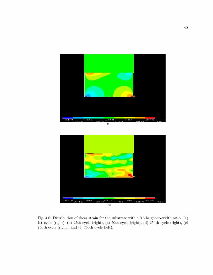
68

Fig. 4.6: Distribution of shear strain for the substrate with a 0.5 height-to-width ratio: (a)1st cycle (right), (b) 25th cycle (right), (c) 50th cycle (right), (d) 250th cycle (right), (e)750th cycle (right), and (f) 750th cycle (left).

69

Fig. 4.6 continued.

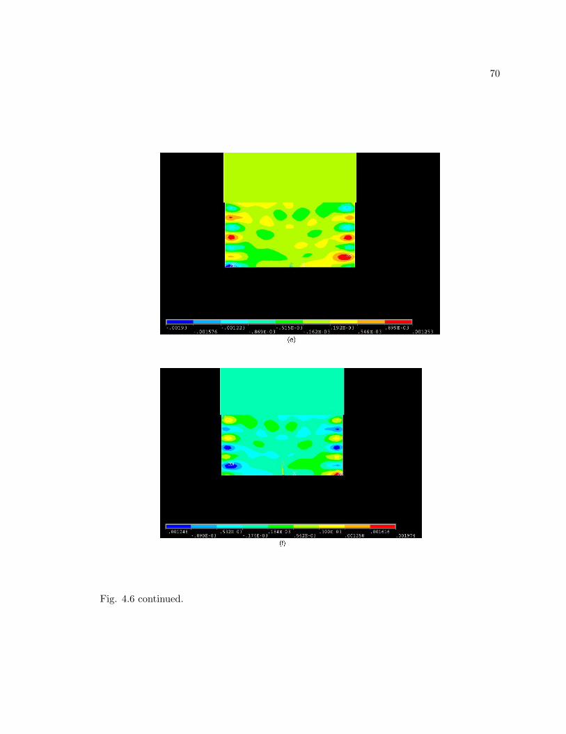
70

Fig. 4.6 continued.

71

Fig. 4.7: Distribution of shear strain at the 750th cycle for substrate with different height-to-width ratios (H/W): (a) H/W=0.25, (b) H/W=0.5, (c) H/W=0.75, (d) H/W=1.0, (e)H/W=1.5, and (f) H/W=2.0.

72

Fig. 4.7 continued.

73

Fig. 4.7 continued.

74

Fig. 4.8: Interface average shear strain vs. height-to-width ratio at the 750th cycle.

4.4 Validation

The simulated friction distributions have confirmed and explained the experimental

observation that ultrasonic consolidation cannot be achieved for free standing substrates

with a height-to-width ratio higher than 1.0. However, the simulation has not answered

why the friction stress decreases to below the critical level for bond formation if the height

of the substrate is greater than a certain value. In addition, the numerical simulation has

not provided an explanation for the banded stress/strain distributions in the substrate.

To understand the wave interference during ultrasonic consolidation and to provide

a validation of the FEM model, a vibration analysis of a 2-D ultrasound wave model is

conducted. Consider a square domain with dimensions of a × a, where a is the half width

of the substrate in the FEM model (Figure 4.9). Let u and v represent the displacements

in the x and y directions, respectively. The edge (y = 0) is fixed, whereas the edge (x = 0)

is free. Based on the FE simulation results, the edge (x = a) is anti-symmetric. The edge

(y = 1) is forced to oscillate along the X-direction at a frequency of 20 kHz with different

vibration amplitudes. To simplify this vibration problem, a free vibration condition with a

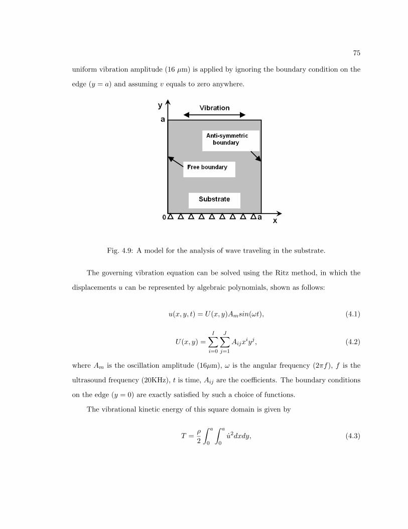
75

uniform vibration amplitude (16 µm) is applied by ignoring the boundary condition on the

edge (y = a) and assuming v equals to zero anywhere.

Fig. 4.9: A model for the analysis of wave traveling in the substrate.

The governing vibration equation can be solved using the Ritz method, in which the

displacements u can be represented by algebraic polynomials, shown as follows:

u(x, y, t) = U(x, y)Amsin(ωt), (4.1)

U(x, y) =

I∑i=0

J∑j=1

Aijxiyj , (4.2)

where Am is the oscillation amplitude (16µm), ω is the angular frequency (2πf), f is the

ultrasound frequency (20KHz), t is time, Aij are the coefficients. The boundary conditions

on the edge (y = 0) are exactly satisfied by such a choice of functions.

The vibrational kinetic energy of this square domain is given by

T =ρ

2

∫ a

0

∫ a

0u2dxdy, (4.3)

76

where ρ is the mass per unit volume and dot(·) represents the time derivative. Substituting

Equation 4.1 into 4.3, the maximum kinetic energy during a full vibration cycle is

Tmax =A2mρω

2

2

∫ a

0

∫ a

0U2dxdy. (4.4)

The strain energy during oscillation is

V =1

2

∫ a

0

∫ a

0(σxεx + τxyγxy)dxdy, (4.5)

where σx and εx are the normal stress and strain, τxy and γxy are the shear stress and strain,

respectively.

Constitutive stress-strain and strain-displacement equations are

σx =νEεx

(1 + ν)(1− 2ν), τxy = Gγxy, (4.6)

εx =∂u

∂x, γxy =

∂u

∂y, (4.7)

where ν is Poisson’s ratio, E is Young’s modulus, G is the shear modulus. The maximum

strain energy during an oscillation cycle can be given as a function of U(x, y) by using

Equations 4.1, and 4.5-4.7.

The functional Lmax (≡ Tmax − Vmax) is minimized by

∂Lmax∂Aij

= 0 (i = 0 . . . I; j = 1 . . . J). (4.8)

After the minimization of Lmax, the yielded set of (I + 1)J homogeneous, linear, alge-

braic equations are solved for the nontrivial solutions under the condition of I = J = 9.

The obtained displacement u is applied to calculate the shear strain, plotted in Fig-

ure 4.10. The vibration model has provided a steady distribution of shear strain for the

substrate with a 0.5 H/W ratio, which corresponds to that in Figure 4.6e and f. By com-

parison, two common characters are found: (1) Both positive and negative shear strain

77

concentrations occur in the substrate. (2) After half of the vibration period, those strain

concentrations will switch their locations, while keeping their magnitude almost unchanged.

A good agreement (with the maximum difference of 13.0%) is also found by a quantitative

comparison of those strain concentrations closest to the contact surface for the FEM and

vibration models, shown in Table 4.2. The banded shear strain distributions and cyclic

strain concentrations are indeed caused by the ultrasound wave interference in the sub-

strate. This wave-based understanding helps to explain many process problems and reveal

the mechanisms of ultrasonic consolidation.

Fig. 4.10: Distribution of shear strain for the substrate with a 0.5 height-to-width ratio:(a) sonotrode moves to the right, and (b) sonotrode moves to the left.

78

Table 4.2: Comparison of Shear Strain Between FEM and Vibration Models (H/W=0.5)

Shear Strain (right) Shear Strain(left)

FEM Model -0.00104 +0.00108

Vibration Model -0.00094 +0.00094

Difference (%) 9.6 13.0

79

Chapter 5

Bond Strength Characterization and Improvement of UW

Parts

5.1 Background of Bond Strength Determination

The overall strength of a laminated structure depends critically on the bond strength

between laminated layers. Bond strength measurement has been widely employed to e-

valuate strength for thin film coating, dental adhesion, and composite fabrication. There

are several methods to experimentally evaluate the bond strength for laminated structures.

These methods can be broadly classified into five categories depending upon the debonding

mode: (a) tensile test (pull-off test), (b) bending test, (c) peel test, (d) scratch test, and

(e) ultrasonic test.

The tensile test [60] is the most commonly used method for the bond strength mea-

surement of thin layers. An increasing tensile force is applied perpendicular to the bonding

interface until the interface fails. Some criteria, such as the maximum force or area of

detachment, are measured and used to evaluate the bond strength. Two requirements of

this method include: (1) the interface bond strength must be lower than the strength of the

adhesive media with which an extension can be joined to the thin layer for gripping and

(2) a uniform load should be applied across the interface. Two drawbacks for the direct

tensile test are: (a) a tensile test involves a complex mixture of tensile and shear forces that

make the results difficult to interpret and (b) a tensile test is limited by the strength of the

adhesive media.

In the bend test [61, 62], a load is applied to a sample fixed in a support. Crack

nucleation and propagation are detected from the disruption of the load-deflection curve or

by an acoustic emission detector. In the peel test [63,64], a layer is peeled from a substrate

80

by a peeling load. For both the bend and peel tests, alignment of the specimen with the

axis of the testing machine is not required, but both tests are limited to soft coatings or

films. The peel test has less substrate distortion resulted in the test than the tensile and

bend test. However, the results of peel tests are difficult to interpret, and are not directly

comparable with the other bond strength testing methods, unless a layer can be completely

debonded from the substrate. This limits the peel test to be suitable for layers with poor

bond strength.

In the scratch test [65–67], an increasing load is applied to scratch a layer by an

indenter tip. The critical load for failure is recorded for the analysis of bond strength. In

the ultrasonic test [68–72], the ultrasonic wave is reflected from the interface when a bond

is not perfect. The amplitude of the reflected wave is measured and correlated with the

bond strength. The difficulty with these two methods is the interpretation of results and

qualitative correlation to the bond strength. The difficulty arises from the many variables

involved in the measurement and analysis procedures. Some other methods, such as lateral

force-sensing microindentation, and laser spallation tests have also been developed for the

evaluation of bond strength [73,74].

We propose a new method for bond strength measurement, the push-pin experiment

and finite element simulation (PEFE) for laminated structures. PEFE has the following

advantages: (a) It is simple to set up, and efficient to test. (b) No adhesive is required for

specimen extension, therefore there is no limitation due to the adhesive media or interface

strength. (c) For multilayer structures, it has the capability of performing the bond strength

measurement of each layer. (d) It is straight forward to interpret the experimental results by

decoupling the shear force and obtaining the bond strength, with the help of finite element

analysis. (e) A master calibration curve can be prepared to identify bond strength.

Bond strength is a critical issue that can greatly influence the development of UW and

its expansion in existing and new fields. However, there have been no bond strength data

from direct measurements on UW structures. The reason seems to be the lack of a suitable

method to evaluate the bond strength between bonded layers. Attempts to conduct tensile

81

testing for the bond strength have not been successful, because the specimen fails at the

grips, and it is difficult to control the failure location to a specific bond interface. The

motivation for the current work, as well as the first application, has been to measure the

bond strength of structures built by UW.

5.2 Methodology of PEFE

PEFE is defined as push-pin experiment and finite element simulation to determine

the bond strength measurement for laminated structures. PEFE involves the following

steps: (1) conduct the push-pin experiment and record the force and displacement data; (2)

develop a layer-structured FE model with the same dimensions to simulate the push-pin

experiment; (3) try different property coefficients for the bond zone until the curve of force

versus displacement from the simulation match those from the experiment; and (4) pick the

maximum stress normal to the bonded areas from simulation results as the bond strength.

5.2.1 Push-pin Experiment

Experiment Setup

Figure 5.1 shows the schematic and setup of the push-pin experiment on the GleebleTM

1500D thermomechanical simulator. In the push-pin test, the left surface of the baseplate

is fixed and a hole is machined from the right surface of the baseplate along the direction

normal to the bond areas. The depth of the hole is determined by the depth of the interface

of which the bond strength is to be measured. A uniform load is applied with a given

strain rate on the specimen by a push rod until the specimen fails. The history of force and

displacement is recorded.

Specimen Design and Test Procedure

The push-pin experiment is designed to study the bond strength of UW, as influenced

by process parameters in UW. The controlled process parameters include the sonotrode

vibration amplitude, normal pressure, and sonotrode’s travel velocity. For this study, four

82

Fig. 5.1: Schematic of the push-pin experiment (a), and setup for the push-pin experimenton the Gleeble (b).

levels are chosen for each process parameter (Table 5.1), while keeping other process param-

eters constant. Samples are built on the SolidicaTM Formation UW system. The geometry

of the multilayered buildup for the process parameter study is 22.9 mm wide, 25.4 mm long,

and 16-layers high. The raw material in foil format is Al3003-H18 aluminum strip 0.1 mm

thick, and 23.9 mm wide. A hole with 12.4 mm diameter was machined into the specimen.

The diameter of push rod is 12.3 mm. The displacement rate used in the push-pin test is

0.42 mm/s. The tests are conducted on the GleebleTM 1500D thermomechanical simulator.

To provide the necessary data for simulation, the mechanical properties and coefficient of

friction of the raw aluminum foil Al3003-H18 have also been measured on the Gleeble.

PEFE allows bond strength measurement on bond interfaces through different depths

of the hole machined into the substrate. This unique characteristic of PEFE provides a

reliable way to perform bond strength measurement for parts with a very small number of

layers. One layer buildup is able to be tested, with a backup metal plate glued to the top

surface of the layer to prevent the push through by the push pin.

83

Table 5.1: Process Parameters for Ultrasonic Welding

Parameters Level 1 Level 2 Level 3 Level 4

Sonotrode vibration amplitude (µm) 12 16 20 24Sonotrode normal pressure (N) 800 1000 1400 1800Sonotrode travel velocity (m/min) 1.02 1.27 1.42 1.53

Note: The pressure and velocity are 1800 N and 1.42 m/min for the study ofamplitude; the amplitude and velocity are 16 µm and 1.42 m/min for the studyof pressure; the pressure and amplitude are 1800 N and 16 µm for the study ofvelocity.

Fig. 5.2: Force vs. displacement curves from push-pin experiments on specimens madewith varying UC process parameters: (a) vibration amplitude, (b) normal pressure, and (c)sonotrode’s travel velocity.

84

Experimental Results

The results of push-pin experiments for the study of UW process parameters are shown

in Figure 5.2. It can be seen that applied force increases nonlinearly with displacement. The

force reaches its peak value and drops down quickly. Parts built by UW show brittle fracture

normal to bonded areas with low ductility. A typical tested push-pin specimen is shown

in Figure 5.3. Most of the specimens fracture along the bond line by separation of the foil

interface. A fractography with porous features can be observed, indicating only a fraction

of the bond interface has been bonded. The slopes and peak values on these curves of force

versus displacement are revealing the real property differences among samples. Higher s-

lope and peak value represent greater material stiffness and fracture strength. These results

indicate that the push-pin experiment is a sensitive method for bond strength measurement.

Fig. 5.3: Typical tested push-pin specimen.

The push-pin experiment also improves the understanding of process parameters on

bonding strength. Among the selected process parameters, vibration amplitude has the

most significant influence on the slope and peak value of force versus displacement curve.

That means vibration amplitude is a critical factor that determines properties of parts

built by the UW process. Larger vibration amplitude resulted in a stronger UW bond,

which is shown by the slope and peak value increasing with vibration amplitude. In the

selected range of normal pressure and sonotrode’s travel velocity, the curves of force versus

85

displacement show similar slopes, but different peak values. This implies that the major

effect of normal pressure and travel velocity is on the fracture strength, not the structure

stiffness. The peak values showed a nonlinear relation with parameters of normal pressure

and travel velocity. Experiment and simulation of the UW process showed that too large

or too small of a normal pressure, and too high of a travel velocity will produce defective

UW bonding. On the other hand, too slow of a velocity will reduce the efficiency of the

manufacturing process. That is shown in the results (Figure 5.2b-c). It is seen that the peak

force values for 800 N pressure and 1.53 m/ min velocity are smaller than the optimized

process parameters, which are 1800 N and 1.42 m/min, respectively.

5.2.2 Finite Element Simulation

The Finite Element Model

Due to the symmetry of specimens, a 2D FE model with a layered structure has been

developed, based on the commercial ANSYS software, to simulate the push-pin experiment.

Figure 5.4 shows the layered and meshed models. In the layered part, narrow strips are

located between layers to simulate the bond zones. The layered part and bond zones have

been finer meshed. The dimensions and number of layers are the same as those in push-pin

specimen in order to match the experimental and simulation results. The bond zone has

been estimated to be 10-20 µm thick based on microstructure observation. Since the bond

zones are not as strong as the layers, they are assumed to have a proportion of the properties

of raw material. Proportional coefficients of properties are used to correlate the unknown

properties of the bond zones with those of the raw material.

In simulation, the fixed and axial symmetric boundary conditions are used on the edges

of AB and DE, respectively. A bilinear kinematic hardening rule has been used to simulate

the nonlinear material behavior. A load with the same loading rate as in the push-pin

experiment is uniformly applied on the edge of CD (Figure 5.4). Different combinations of

property coefficients of elastic modulus, yield stress, and work hardening for the bond zones

were tested until the curve of force versus displacement from FE simulation matches that

86

Fig. 5.4: Finite element model of the push-pin specimen (a), and meshed model (b).

from push-pin experiment. Therefore, the bond strength can be identified by this FE-based

“experiment”.

Simulation Results

From the FE simulation results, the stress distribution along the edge CD is calculated

for each displacement. Then multiplying the cross section area of the push rod, the average

force on edge CD is calculated for all the displacement levels. The coefficients of elastic

modulus used in simulations for different parameter sets are shown in Table 5.2, which

is found to be the most sensitive in changing the shape of the force versus displacement

curve. Figure 5.5 shows the comparison of force versus displacement from experiment and

simulation for all the parameter sets. It is clearly seen that, when the appropriate bond

strength properties are fed to the FE model, a matching curve can be achieved. The

87

simulation stops at the peak force, based on the assumption that the peak force is the

onset of failure. After the peak force is reached, the crack will propagate quickly and the

resistance will decrease.

Table 5.2: Coefficients of Elastic Modulus for the Bond Layer

Vibration Amplitude (µm) 12 16 20 24

Coefficient (×10−4) 1.1 2.8 3.3 5.0

Normal Pressure (N) 800 1000 1400 1800

Coefficient (×10−4) 1.9 2.4 2.5 2.8

Travel velocity of sonotrode (m/min) 1.02 1.27 1.42 1.53

Coefficient (×10−4) 2.9 2.4 2.8 2.5

The von Mises yield criterion is used in this nonlinear simulation of FE model and the

typical distribution of von Mises strain is shown in Figure 5.6a. The maximum von Mises

strain is located at the corner of the machined inner hole. In the push-pin experiment, all

specimens fail from the corner of the machined inner hole. Therefore, the depth of the hole

can accurately determine the location of the failure. The distribution of von Mises strain

confirms this experimental observation.

The debonding process is a complicated effects of normal and shear stresses on the

fracture plane. However, these effects can be simplified by PEFE, because the stress normal

to the bond areas is more importantly than the other stress components. This means that

this stress will most likely dominate the crack propagation process. This can be proven

by the stress distribution normal to the bond areas, shown in Figure 5.6b. This stress

distribution is similar to that of the von Mises plastic strain, and the maximum tensile

stress is also located at the corner bonding interface. Therefore, the stress data obtained

from the FE simulation, which match the push-pin experiment data, can be used to evaluate

the bond strength.

88

Fig. 5.5: Comparison of force vs. displacement curves from the push-pin experiment andfrom the FE simulation for specimens made using various process parameters: (a) vibrationamplitude, (b) normal pressure, and (c) sonotrode’s travel velocity.

89

Fig. 5.5 continued.

Fig. 5.6: A typical von Mises strain distribution near the corner of the push-pin hole (a)and a typical z-direction (specimen height direction) stress σzz distribution at the samelocation (Unit : Pa) (b).

90

5.2.3 Determination of Bond Strength by PEFE

The debonding at the interface involves the coupling of stresses that make the failure

analysis for layered structures difficult. Brewer and Lagace [75] proposed a general criterion,

the quadratic delamination criterion (QDC), for the prediction of interface debond that

takes the coupling effect of normal and shear stresses into account. Based on QDC, the

onset of interfacial failure can be predicted with

( σxzZsx

)2+

(σyzZsy

)2

+

(σtzzZt

)2

+

(σczzZc

)2

= 1 (5.1)

where σij = average of a stress component;

Zt = tensile interlaminar normal strength;

Zc = compressive interlaminar normal strength;

Zsx = interlaminar shear strength for σxz stresses; and

Zsy = interlaminar shear strength for σyz stresses.

When one stress component, normal or shear stress, is dominant in the failure process,

Equation 5.1 can be significantly simplified. We assume that the debond failure in UW

specimens is caused mainly by normal tensile stress at the failure interface. Therefore, all

terms on the left hand side of Equation 5.1 can be ignored, except the Zt term. With

this simplification Equation 5.1 becomes σtzz = Zt, the maximum stress failure criterion.

Compared with QDC, the maximum stress failure criterion [76,77] is an effective and popular

approach for engineering failure analysis. In the push-pin experiment, the peak force has

been found and taken as the starting point for debonding failure. The maximum stress σtzz

corresponding to the peak force is calculated from the FE simulation and taken as the bond

strength Zt.

Figure 5.7 shows the determined bond strength Zt of UW specimens using the proposed

PEFE method. The highest bond strength for parts made with the parameters discussed

in this study is identified to be 180 MPa, which is 75% of the UTS of the raw material. For

the first time, the bond strength of UW processed components can be positively determined

using PEFE.

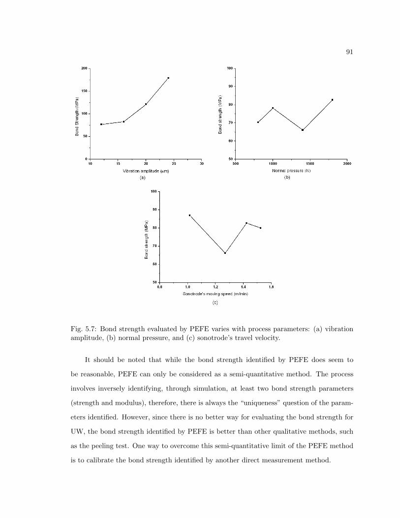
91

Fig. 5.7: Bond strength evaluated by PEFE varies with process parameters: (a) vibrationamplitude, (b) normal pressure, and (c) sonotrode’s travel velocity.

It should be noted that while the bond strength identified by PEFE does seem to

be reasonable, PEFE can only be considered as a semi-quantitative method. The process

involves inversely identifying, through simulation, at least two bond strength parameters

(strength and modulus), therefore, there is always the “uniqueness” question of the param-

eters identified. However, since there is no better way for evaluating the bond strength for

UW, the bond strength identified by PEFE is better than other qualitative methods, such

as the peeling test. One way to overcome this semi-quantitative limit of the PEFE method

is to calibrate the bond strength identified by another direct measurement method.

92

Based on Figure 5.7a, an increasing vibration amplitude increases the bond strength

and it has more significant effect on bond strength/formation than the other two parameters

(pressure and travel velocity). In the actual manufacturing process of UW, the optimum

parameter set used were 16 µm vibration amplitude, 1800 N normal pressure, and 1.42

m/min travel velocity. In Figure 5.7b, normal pressure of 1800 N resulted in the best bond

strength, while the lowest pressure of 800 N resulted in the worst bond strength. Based on

our understanding of the UW process, to a high normal pressure will decrease bond strength,

because the vibrational motion of the parts is constrained, and not enough friction heat will

be generated. Thus, intermediate normal pressure, in the range of 1800 N, is the optimal

for higher quality UW bonding. Figure 5.7c shows that the lowest travel velocity has the

highest bond strength. Although the lowest moving velocity is optimal for bond formation,

it also reduces the working efficiency. Therefore, considering the bond strength and working

efficiency, 1.42 m/min is the optimal choice for the range of parameters considered in this

study.

5.2.4 Correlation of Bond Strength by PEFE with Percentage of Bonded Area

Figure 5.8 shows the typical morphology of fractured surfaces for both high and low

quality UW bonding conditions discussed in this study. A difference in the percentage of

bonded area exists for these two bonding conditions. Most of the area is bonded for the

better UW bonds, while large un-bonded areas exist in the low quality UW bonds. The

percentage of bonded area is a reliable way of evaluating the bond formation and bond

strength. The bulk bond strength can be predicated by the averaged percentage of bonded

area of the entire bonded surfaces. The bond strength in a local region can also be evaluated

from the percentage of bonded area of that local region. The bulk averaged percentage of

bonded areas have been measured with digital images of fractured surfaces, and converted

to bond strength. The bond strength from area measurements is defined as the averaged

percentage of bonded area times raw material’s UTS. The results of bond strength evaluated

by percentage of bonded areas are plotted in Figure 5.9. Comparing Figures 5.7 and 5.9, the

bond strength provided by these two approaches are showing the same trend for all three

93

Fig. 5.8: Typical feature of fractured surfaces: (a) 91.6% bonded area, and (b) 74.9%bonded area.

process parameters. The similarity between these two sets of results is a strong validation

for the PEFE method. The bond strength is probably over-evaluated by the percentage of

bonded area method. It should be recognized that the UTS of the raw material used in the

bond strength calculation from area is higher than the real bond strength.

Figure 5.10a shows the relation between the bond strength by PEFE and percentage

of bonded area. With this curve, an estimate of bond strength can also be obtained by

conducting a bonded area measurement of UW specimens. The bond strength increases

rapidly when the percentage of bonded area is over 90%. This trend can be explained

by a basic fracture mechanics analysis. The general form of the Griffith [78] equation is

sf =

√2Ewf

πa , where σf is failure stress, E is elastic modulus, wf is fracture energy, which

could include plastic, viscoelastic, or viscoplastic effects, depending on materials, and a is

half of the crack length. The failure stress is proportional to√

1a , when assuming that E

and wf are constants for a given material. In PEFE, the un-bonded area can be considered

as a crack, so an equivalent crack length (aeqv) is calculated from the percentage of bonded

area by

94

Fig. 5.9: Bond strength evaluated by bonded area to total area ratio varying with pro-cess parameters: (a) vibration amplitude, (b) normal pressure, and (c) sonotrode’s travelvelocity.

aeqv =1

2L

√A(1− rb) (5.2)

where A is total cross section area, rb is percentage of bonded area, and L is width of

cross section.

Substituting the crack length a in the Griffith equation with aeqv, the equivalent fracture

strength for the defect-containing UW specimens can be written as

95

Fig. 5.10: Bond strength by PEFE vs. percentage of bonded area (a), and bond strengthas a function of the equivalent crack length, with a comparison between strength obtainedusing PEFE and strength predicted using Equation 5.3 (b).

sf =

√2Ewfπaeqv

(5.3)

If a constant fracture energy wf is assumed, the curve of sf (i.e., bond strength) versus

aeqv can be fitted to correlate with the bond strength determined by PEFE (Figure 5.10b).

When the normalized equivalent crack length is longer than 0.25, the bond strength governed

by Equation 5.2 matches well with that by PEFE. Although assumed as a constant, the

fracture energy wf should be viewed as a parameter, which may affect the bond strength.

5.3 Pressurized Post-weld Heat Treatment (PWHT)

Attempting to solve the problem of poor vertical bond strength of UW parts, a pres-

surized post-weld heat treatment is proposed. First, a systematic experimental matrix

of PWHT is designed and conducted to study the coupled influences of temperature and

time on bond strength. Based on the results of traditional PWHT and diffusion bonding

mechanism, a series of pressurized PWHT tests have been conducted to find out the po-

tential of bond strength improvement and the optimum parameter set, including pressure,

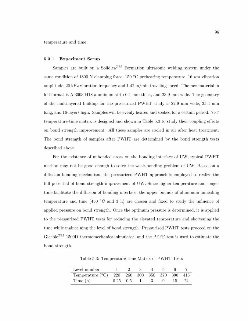
96

temperature and time.

5.3.1 Experiment Setup

Samples are built on a SolidicaTM Formation ultrasonic welding system under the

same condition of 1800 N clamping force, 150 ◦C preheating temperature, 16 µm vibration

amplitude, 20 kHz vibration frequency and 1.42 m/min traveling speed. The raw material in

foil format is Al3003-H18 aluminum strip 0.1 mm thick, and 23.9 mm wide. The geometry

of the multilayered buildup for the pressurized PWHT study is 22.9 mm wide, 25.4 mm

long, and 16-layers high. Samples will be evenly heated and soaked for a certain period. 7×7

temperature-time matrix is designed and shown in Table 5.3 to study their coupling effects

on bond strength improvement. All these samples are cooled in air after heat treatment.

The bond strength of samples after PWHT are determined by the bond strength tests

described above.

For the existence of unbonded areas on the bonding interface of UW, typical PWHT

method may not be good enough to solve the weak-bonding problem of UW. Based on a

diffusion bonding mechanism, the pressurized PWHT approach is employed to realize the

full potential of bond strength improvement of UW. Since higher temperature and longer

time facilitate the diffusion of bonding interface, the upper bounds of aluminum annealing

temperature and time (450 ◦C and 3 h) are chosen and fixed to study the influence of

applied pressure on bond strength. Once the optimum pressure is determined, it is applied

to the pressurized PWHT tests for reducing the elevated temperature and shortening the

time while maintaining the level of bond strength. Pressurized PWHT tests proceed on the

GleebleTM 1500D thermomechanical simulator, and the PEFE test is used to estimate the

bond strength.

Table 5.3: Temperature-time Matrix of PWHT Tests

Level number 1 2 3 4 5 6 7

Temperature (◦C) 220 260 300 350 370 390 415

Time (h) 0.25 0.5 1 3 9 15 24

97

5.3.2 Experiment Results

PWHT

Based on the obtained systematic bond strength data, a 2-D map is plotted (Figure

5.11), which clearly exhibits the influence of temperature and time of PWHT on the bond

strength. The lower left corner represents the low bond strength zone, corresponding to

the low-temperature and short-period PWHT conditions. On the contrary, the upper right

corner is the height bond strength zone, resulting from the opposite conditions. With the aid

of this 2D map, the quantitative bond strength can be easily determined for an arbitrary

combination of temperature and time within the studied range. The bond strength is

increased by 35% from the as-welded condition using the best PWHT condition.

Since the UW bonding interface is severely plastic-deformed and residual stress/strain

concentrated, the annealing influence of PWHT causes the stress relief and reduces the

effect of strain hardening, which result in the decrease of hardness, but the improvement

of ductility. After the classification of failure mode for the PWHT samples after PEFE

testing, a 2D map of failure mode has been plotted, shown in Figure 5.12, and the critical

PWHT condition of failure mode change is marked by a dash line. The PWHT condition

of higher temperature and longer time has more potential to generate the ductile failure.

Typical evolutions of peak load vs. displacement for the brittle and ductile failure modes

are also shown in Figure 5.12. For the UW parts with a laminate structure, the ductile

failure mode is characterized by a debonding surface across several layers, while the brittle

failure mode occurs on a single bonding layer.

Pressurized PWHT

Although the bond strength of UW parts can be improved by the traditional PWHT

method (35% from the as-welded condition), it is still far below the strength of the base

material (only 48%). To achieve even higher bond strength, pressurized PWHT tests are

conducted, and results are shown in Figures 5.13-5.16. Under the PWHT condition of

450 ◦C and 3 h, the bond strength increases with applied pressure (≤2.5 MPa) initially,

98

Fig. 5.11: 2D temperature-time bond strength map after PWHT (Unit: MPa).

Fig. 5.12: 2D temperature-time failure mode map after PWHT.

and remains constant at higher stresses (>2.5 MPa), illustrated in Figure 5.13. Through

applying pressure to the UW parts during PWHT tests, the bond strength can be modified

significantly, up to 96% of the strength of the base material. When the applied pressure

is above 2.5 MPa, the sample geometry starts to be destroyed permanently (Figure 5.14).

99

Considering both the bond strength and sample geometry, the pressure of 2.5 MPa is chosen

as the optimum pressure value, which is applied to the rest of the tests determining the

optimum temperature and time. The bond strength keeps increasing with temperature

(Figure 5.15). Therefore, 450 ◦C is a good choice as the optimum temperature value. In

Figure 5.16, the PWHT time can be shortened from 3 h to 1.5 h, while maintaining the

bond strength level. Finally, the optimum parameters of pressurized PWHT tests are 2.5

MPa pressure, 450 ◦C temperature and 1.5 h time.

Fig. 5.13: Variation of bond strength after pressurized PWHT with pressure.

Fig. 5.14: Variation of buildup deformation after pressurized PWHT with pressure.

100

Fig. 5.15: Variation of bond strength after pressurized PWHT with temperature.

Fig. 5.16: Variation of bond strength after pressurized PWHT with time.

101

Chapter 6

Conclusions and Future Work

1. A new fully coupled thermomechanical finite element model has been developed to

simulate the ultrasonic metal welding process. Insight has been gained on the evo-

lution and interactions between the in-process thermal- mechanical variables. The

model is able to explain experimental observations on the effect of process parameters

on bond formation. The von Mises plastic strain obtained from the simulation has

been quantitatively verified by experimentally measured data and correlated with the

measured bonded area of ultrasonic joints. A possible mechanism for bond forma-

tion is proposed. Ultrasonic welding forms the bond through the following process:

ultrasonic vibration generates shear stress, sliding, and heat at the interface through

friction; the heat lowers the mechanical properties of the material, which enhances

localized plastic deformation; and more plastic deformation generates more heat in

addition to frictional heat. It is the severe, localized, plastic deformation at the bond

region that is believed to be the major phenomenon for bond formation in ultrasonic

welding.

2. With the increased substrate height, the amplitude of contact frictional stress decreas-

es, while that of contact interface displacement increases. The reason for the decrease

in the frictional stress at the contact interface for certain substrate heights is caused

by the wave interference occurring in the substrate, which has been validated by an

analytical vibration model. The formation of banded and cyclic stress-strain maxima

in the substrate is also caused by superposition of vibrations.

3. A push-pin type, combined experimental and numerical method for evaluation of

bond strength of laminated structures has been developed. The new method has been

102

validated by experimental bonded area data, and has been successfully applied to

laminated structures produced using UW.

4. Bond strength for different UW parameter combinations has been evaluated. The best

bond strength produced using the set of ultrasonic process parameters in this study

is 75% of the UTS of the base material. An increase of vibration amplitude of the

sonotrode will increase the bond strength. There is an optimized sonotrode pressure

level for bond strength; both low and high pressures will cause a decrease in bond

strength. Lower travel velocity of the sonotrode will generate higher bond strength.

5. PWHT tests have been conducted on the UW parts to explore the potential of bond

strength improvement. Influences of PWHT temperature and time on bond strength

are analyzed and illustrated in a 2D map of bond strength. Under the optimum PWHT

condition (temperature and time only), the bond strength can be improved by 35%

from the as-welded condition. The pressurized PWHT approach is originally proposed

to improve the bond strength of UW parts. The results show that the modified bond

strength, up to 96% of the strength of the base material, can be achieved under the

optimum parameters of 2.5 MPa pressure, 450 ◦C temperature and 1.5 h time.

The results in this dissertation provide a strong foundation for future work in the mech-

anism study of ultrasonic metal welding. One area is in the long-term thermomechanical

fully coupled simulation of bond formation process, in which the simulation of minimum

3000 vibration cycles is suggested. The results of plastic deformation at the bonding sur-

face for the long-term simulation should be compared and correlated with the bonded area

ratio. Another area is in applying the theory of dynamic recrystallization to quantitatively

explain the generation of nano-sized grains at the bonding interface, combined with thermo-

mechanical numerical results from FE simulation. It is also required to develop a method

for directly measurements of the strain/stress or temperature during the bonding process

to validate the numerical model of ultrasonic welding and to help the interpretation of the

bonding mechanisms.

103

References

[1] Ueoka, T. and Tsujino, J., “Welding Characteristics of Aluminum and Copper PlateSpecimens Welded by a 19 kHz Complex Vibration Ultrasonic Seam Welding System,”Japanese Journal of Applied Physics, Part 1 , Vol. 41, No. 5B, 2002, pp. 3237–3242.

[2] Vries, E., Mechanics and Mechanisms of Ultrasonic Metal Welding , Ph.D. thesis, OhioState University, Columbus, 2004.

[3] White, D. R., “Ultrasonic Consolidation of Aluminum Tooling,” Advanced Materials& Processes, Vol. 161, No. 1, 2003, pp. 64–65.

[4] Harman, G. G. and Albers, J., “The Ultrasonic Welding Mechanism as Applied toAluminum- and Gold-Wire Bonding in Microelectronics Aluminum- and Gold-WireBonding in Microelectronics,” IEEE Transactions on Parts, Hybrids, and Packaging ,Vol. PHP-13, No. 4, December 1977, pp. 406–412.

[5] Grewell, D. A., “A Prototype ‘Expert’ System for Ultrasonic Welding of Plastics,”Plastics Engineering (N. Y.), , No. 55, 1999, pp. 33–37.

[6] Wagner, G., Walther, F., Nebel, T., and Eifler, D., “Glass/Glass Joints by UltrasonicWelding,” Glass Technology , , No. 44, 2003, pp. 152–155.

[7] Matsuoka, S. I., “Ultrasonic Welding of Ceramics/Metals Using Inserts,” Journal ofMaterial Processing Technology , Vol. 75, No. 1-3, 1998, pp. 259–265.

[8] Kong, C. Y., Soar, R. C., and Dickens, P., “An Investigation of the Control Parametersfor Aluminium 3003 under Ultrasonic Consolidation,” Proceedings of Solid FreeformFabrication Symposium, Austin, TX, 2002, pp. 199–210.

[9] White, D. R., “Ultrasonic Object Consolidation System and Method, United Statespatent # 6,463,349,” Tech. rep., 2002.

[10] Elangovan, S., Semeer, S., and Prakasan, K., “Temperature and Stress Distributionin Ultrasonic Metal Welding - An FEA-based Study,” Journal of Materials ProcessingTechnology , Vol. 209, 2009, pp. 1143–1150.

[11] Kong, C. Y. and Soar, R. C., “Fabrication of Metal-matrix Composites and AdaptiveComposites Using Ultrasonic Consolidation Process,” Materials Science and Engineer-ing A, Vol. 412, 2005, pp. 12–18.

[12] Yang, Y., Ram, J., and Stucker, B., “An Experimental Determination of OptimumProcessing Parameters for Al/SiC Metal Matrix Composites Made Using UltrasonicConsolidation,” Journal of Engineering Materials and Technology - Transactions ofthe ASME , Vol. 129, No. 4, 2007, pp. 538–549.

104

[13] Yang, Y., Ram, G. J., and Stucker, B., “Bond Formation and Fiber Embedment DuringUltrasonic Consolidation,” Journal of Materials Processing Technology , Vol. 209, 2009,pp. 4915–4924.

[14] Doumanidis, C. and Gao, Y., “Mechanical Modeling of Ultrasonic Welding,” WeldingJournal , Vol. 83, No. 4, 2004, pp. 140S–146S.

[15] Ginzburg, S., Mitskevich, A., and Nosov, Y., “Formation of the Joint in UltrasonicWelding,” Welding Production, Vol. 13, No. 5, May 1967, pp. 45–47.

[16] Chang, U. I. and Frisch, J., “On Optimization of Some Parameters in Ultrasonic MetalWelding,” Welding Journal , Vol. 53, No. 1, January 1974, pp. 24–35.

[17] Beyer, W., “The Bonding Process in the Ultrasonic Welding of Metals,” Schweisstech-nik , Vol. 19, No. 1, January 1969, pp. 16–20.

[18] Watanabe, A., Yanagisawa, T., and Sunaga, S., “The Effect of Oxide Film on theStrength of an Ultrasonically Welded Joint and Welding Process - Study of the Ultra-sonic Welding of Dissimilar Metals (2nd Report),” Welding Research Abroad , Vol. 48,No. 2, 2000, pp. 19.

[19] Hazlett, T. and Ambekar, S., “Additional Studies on Interface Temperatures and Bond-ing Mechanism of Ultrasonic Welds,” Welding Journal , May 1970, pp. 196–200.

[20] Kreye, H., “Melting Phenomena in Solid State Welding Processes,” Welding Journal ,Vol. 56, No. 5, May 1977, pp. 154–158.

[21] Harthoorn, J., Ultraonic Metal Welding , Ph.D. thesis, Technical University, Eindhoven,1978.

[22] Heymann, E. and Pusch, G., “Contribution to the Study of the Role of Recrystallizationin the Formation of the Joint in Ultrasonic Welding,” Schweisstechnik , Vol. 19, No. 12,December 1969, pp. 542–545.

[23] Gao, Y. and Doumanidis, C., “Mechanical Analysis of Ultrasonic Bonding for RapidPrototyping,” Journal of Manufacturing Science and Engineering, Transactions of theASME , Vol. 124, No. 2, 2002, pp. 426–434.

[24] Pfluger, A. and Sideris, X., “New Developments in Ultrasonic Welding,” Sampe Quar-terly , Vol. 7, No. 1, October 1975, pp. 9–19.

[25] Zhou, Y., Li, X., and Noolu, N. J., “A Footprint Study of Bond Initiation in Gold WireCrescent Bonding,” IEEE Transactions on Components and Packaging Technologies,Vol. 28, No. 4, 2005, pp. 810–816.

[26] Eaves, A., “Review of the Application of Ultrasonic Vibration to Deforming Metals,”Ultrasonics, Vol. 13, No. 4, 1975, pp. 162–170.

[27] Hansson, I. and Tholen, A., “Plasticity due to Superimposed Macrosonic and StaticStrains,” Ultrasonics, Vol. 16, No. 2, 1978, pp. 57–64.

105

[28] Gao, Y. and Doumanidis, C., “Mechanical Analysis of Ultrasonic Bonding for RapidPrototyping,” Journal of Manufacturing Science and Engineering, Transactions of theASME , Vol. 124, No. 2, 2002, pp. 426–434.

[29] Zhang, C. and Li, L., “A Coupled Thermal-mechanical Analysis of Ultrasonic BondingMechanism,” Metallurgical and Meterials Transactions B , Vol. 40B, 2009, pp. 196–207.

[30] Zhang, C. and Li, L., “A Friction-based Finite Element Analysis of Ultrasonic Consol-idation,” Welding Journal , Vol. 87, No. 7, 2008, pp. 187s–194s.

[31] Huang, C. and Ghassemieh, E., “3D Coupled Thermomechanical Finite Element Anal-ysis of Ultrasonic Consolidation,” Materials Science Forum, Vol. 539-543, 2007, p-p. 2651–2656.

[32] Yadav, S. and Doumanidis, C., “Thermomechanical Analysis of an Ultrasonic RapidManufacturing (URM) System,” Journal of Manufacturing Processes, Vol. 7, No. 2,2005, pp. 153–161.

[33] Ding, Y. and Kim, J., “Numerical Analysis of Ultrasonic Wire Bonding: Part 2. Effectsof Bonding Parameters on Temperature Rise,” Microelectronics Reliability , Vol. 48,2008, pp. 149–157.

[34] Ding, Y., Kim, J., and Tong, P., “Numerical Analysis of Ultrasonic Wire bonding:Effects of Bonding Parameters on Contact Pressure and Frictional Energy,” Mechanicsof Materials, Vol. 38, 2006, pp. 11–24.

[35] Siddiq, A. and Ghassemieh, E., “Thermomechanical Analyses of Ultrasonic Weld-ing Process Using Thermal and Acoustic Softening Effects,” Mechanics of Materials,Vol. 40, 2008, pp. 982–1000.

[36] Siddiq, A. and Ghassemieh, E., “Theoretical and FE Analysis of Ultrasonic Welding ofAluminum Alloy 3003,” Journal of Manufacturing Science and Engineering , Vol. 131,No. 041007, 2009.

[37] Senchenkov, I., Tarasenko, O., Chernyak, B., Kozlov, V., and Frenkel, B., “AcousticContact during the Ultrasonic Welding of Plastics,” Soviet Applied Mechanics (EnglishTranslation of Prikladnaya Mekhanika), Vol. 23, No. 2, 1987, pp. 159–165.

[38] Senchenkov, I., “Vibrational Heating of a Nonlinearly Viscoelastic Rod Interacting witha Viscoelastic Element,” Soviet Applied Mechanics (English Translation of PrikladnayaMekhanika), Vol. 27, No. 5, 1991, pp. 512–519.

[39] Benatar, A. and Gutowski, T., “Ultrasonic Welding of PEEK Graphite APC-2 Com-posites,” Polymer Engineering and Science, Vol. 29, No. 23, 1989, pp. 1705–1721.

[40] Roylance, M., Player, J., Zukas, W., and Roylance, D., “Modeling of Ultrasonic Pro-cessing,” Journal of Applied Polymer Science, Vol. 93, No. 4, 2004, pp. 1609–1615.

[41] Verderber, R., “Implementation of Algorithms for Modeling Ultrasonic Welding,”American Society of Mechanical Engineers, Pressure Vessels and Piping Division (Pub-lication) PVP , Vol. 369, 1997, pp. 229–234.

106

[42] Senchenkov, I. and Zhuk, Y., “Modal Control of Planar Oscillation of SlottedSonotrodes for Ultrasonic Welding of Plastics,” International Conference on Controlof Oscillations and Chaos, Vol. 1, 1997, pp. 133–137.

[43] Mikhailenko, V. and Franovskii, A., “Numerical Modeling of Resonance Modes of theOscillations of an Ultrasonic Electromechanical System with Automatic-frequency Con-trol,” International Applied Mechanics, Vol. 32, No. 11, 1997, pp. 865–870.

[44] Tsujino, J., Ueoka, T., Kashino, T., and Sugahara, F., “Transverse and TorsionalComplex Vibration Systems for Ultrasonic Seam Welding of Metal Plates,” Ultrasonics,Vol. 38, 2000a, pp. 67–71.

[45] Tsujino, J. and Ueoka, T., “Welding Characteristics of Ultrasonic Seam Welding Sys-tem Using a Complex Vibration Circular Disk Welding Tip,” Japanese Journal ofApplied Physics, Part 1: Regular Papers and Short Notes and Review Papers, Vol. 39,No. 5B, 2000b, pp. 2990–2994.

[46] Akay, A., “Acoustics of Friction,” Journal of the Acoustical Society of America,Vol. 111, No. 4, 2002, pp. 1525–1548.

[47] Kong, C., Soar, R., and Dickens, P., “A Model for Welding Strength in UltrasonicallyConsolidated Components,” Proceedings of the Institution of Mechanical Engineers,Part C: Journal of Mechanical Engineering Science, Vol. 219, No. 1, 2005, pp. 83–91.

[48] Ram, G. J., Yang, Y., and Stucker, B., “Effect of Process Parameters on Bond Forma-tion During Ultrasonic Consolidation of Aluminum Alloy 3003,” Journal of Manufac-turing Systems, Vol. 25, No. 3, 2006, pp. 221–238.

[49] Zhang, C., Deceuster, A., and Li, L., “A Method for Bond Strength Evaluation forLaminated Structures with Application to Ultrasonic Consolidation,” Journal of Ma-terials Engineering and Performance, Vol. 18, No. 8, 2009, pp. 1124–1132.

[50] Metals Handbook , Vol. 2, 10th Ed., ASM International, 1990.

[51] Ravichandran, G., Rosakis, A., Hodowany, J., and Rosakis, P., “On the Conversionof Plastic Work into Heat During High-Strain-Rate Deformation,” AIP ConferenceProceedings, Vol. 620, No. 1, July 2002, pp. 557–562.

[52] ANSYS, INC., Release 11.0 Documentation for ANSYS .

[53] Lemaitre, J. and Chaboche, J., Mechanics of Solid Materials, Cambridge UniversityPress, UK, 1990.

[54] Huber, N. and Tsakmakis, C., “Determination of Constitutive Properties from Spher-ical Indentation Data Using Neural Networks - Part II: Plasticity with NonlinearIsotropic and Kinematic Hardening,” Journal of the Mechanics and Physics of Solids,Vol. 47, 1999, pp. 1589–1607.

[55] Armstrong, P. and Frederick, C., “A Mathematical Representation of the MultiaxialBauschinger Effect,” CEGB Report , Vol. No. RD/B/N 731, 1966.

107

[56] Zhang, C. and Li, L., “A Study of DynamicMechanical Behavior of Substrate in Ultra-sonic Consolidation,” The 17th Solid Freeform Fabricaion Symposium, Austin, Texas,2006.

[57] Zhang, C. and Li, L., “Effect of Substrate Dimensions on Dynamics of UltrasonicConsolidation,” Ultrasonics, Vol. 50, 2009, pp. 811–825.

[58] Robinson, C., Zhang, C., Siggard, E., Ram, J., Stucker, B., and Li, L., “MaximumHeight to Width Ratio of Freestanding Structures Built using Ultrasonic Consolida-tion,” The Seventeenth Solid Freeform Fabrication Symposium, August 14-16, 2006Austin, Texas., 2006.

[59] Kong, C., Soar, R., and Dickens, P., “Ultrasonic Consolidation Technique for Embed-ding SMA Fibers with Aluminium Matrices,” Composite Structures, Vol. 66, 2005,pp. 421–427.

[60] Mittal, K. L., “Adhesion Measurement of Thin Films,” Electrocomponent Science andTechnology , Vol. 3, 1976, pp. 21–42.

[61] Atsu, S. and Berksun, S., “Bond Strength of Three Porcelains to Two Forms of Tita-nium Using Two Firing Atmospheres,” The Journal of Prosthetic Dentistry , Vol. 84,No. 5, November 2000, pp. 567–574.

[62] Matsuura, K., Sueoka, N., Kudoh, M., and Ohsasa, K., “Nickel Monoaluminide Coatingon Ultralow-carbon Steel by Reactive Sintering,” Metallurgical and Materials Trans-actions A, Vol. 30, No. 6, June 1999, pp. 1605–1612.

[63] Karbhari, V. M., “Investigation of Bond Between Concrete and Composites: Use ofa Peel Test,” Journal of Reinforced Plastics and Composites, Vol. 15, No. 2, 1996,pp. 208–227.

[64] Love, B. J. and Packman, P. F., “Effects of Surface Modifications on the Peel Strengthof Copper Based Polymer/Metal Interfaces with Characteristic Morphologies,” TheJournal of Adhesion, Vol. 40, No. 2-4, May 1993, pp. 139–150.

[65] Bull, S., Rickerby, D., and Matthews, A., “The Use of Scratch Adhesion Testing for theDetermination of Interfacial Adhesion: The Importance of Frictional Drag,” SurfaceCoating Technology , Vol. 36, No. 1-2, December 1988, pp. 503–517.

[66] Perry, A., “Scratch Adhesion Testing of Hard Coatings,” Thin Solid Films, Vol. 107,No. 2, 1983, pp. 167–180.

[67] Burnett, P. and Rickerby, D., “The Scratch Adhesion Test: An Elastic-Plastic Inden-tation Analysis,” Thin Solid Films, Vol. 157, No. 2, February 1988, pp. 233–254.

[68] Lavrentye, A. and Beals, J., “Ultrasonic Measurement of the Diffusion Bond Strength,”Ultrasonics, Vol. 38, March 2000, pp. 513–516.

[69] Baik, J. and Thompson, R., “Ultrasonic Scattering from Imperfect Interfaces: A Quasi-static Model,” Journal of Nondestructive Evaluation, Vol. 4, No. 3-4, December 1984,pp. 177–196.

108

[70] Fraisse, P., Schmit, F., and Zarembowitch, A., “Ultrasonic Inspection of Very ThinAdhesive Layers,” Journal of Applied Physics, Vol. 72, October 1992, pp. 3264–3271.

[71] Lavrentyev, A. and Rokhlin, S., “Ultrasonic Spectroscopy of Imperfect Contact In-terfaces Between a Layer and Two Solids,” The Journal of the Acoustical Society ofAmerica, Vol. 103, February 1998, pp. 657–664.

[72] Singher, L., “Bond Strength Measurement by Ultrasonic Guided Waves,” Ultrasonics,Vol. 35, No. 4, June 1997, pp. 305–315.

[73] Zhang, H., Chen, Q., and Li, D., “Development of a Novel Lateral Force-sensing Mi-croindentation Technique for Determination of Interfacial Bond Strength,” Acta Ma-terialia, 2004, pp. 2037–2046.

[74] Yuan, J. and Gupta, V., “Measurement of Interface Strength by the Modified LaserSpallation Technique. I. Experiment and Simulation of the Spallation Process,” Journalof Applied Physics, Vol. 74, No. 4, 1993, pp. 2388–2396.

[75] Brewer, J. and Lagace, P., “Quadratic Stress Criterion for Initiation of Delamination,”Journal of Composite Materials, Vol. 22, No. 538-548, 1988.

[76] Gerstle, F., “On the Application of the Maximum Stress Failure Criterion to Off-Axisand Angle-Ply Laminates,” Journal of Composite Materials, Vol. 19, No. 6, 1985,pp. 505–512.

[77] Hart-Smith, L., “Predictions of a Generalized Maximum-shear-stress Failure Criteri-on for Certain Fibrous Composite Laminates,” Composites Science and Technology ,Vol. 58, No. 7, 1998, pp. 1179–1208.

[78] Anderson, T., Fracture Mechanics, 2nd Ed., CRC Press, Inc., Boca Raton, FL, 1995.