Thermomechanical response of steel moment-frame beam ...
572
Lehigh University Lehigh Preserve eses and Dissertations 2012 ermomechanical response of steel moment- frame beam-column connections during post- earthquake fire exposure Wesley J. Keller Lehigh University Follow this and additional works at: hp://preserve.lehigh.edu/etd is Dissertation is brought to you for free and open access by Lehigh Preserve. It has been accepted for inclusion in eses and Dissertations by an authorized administrator of Lehigh Preserve. For more information, please contact [email protected]. Recommended Citation Keller, Wesley J., "ermomechanical response of steel moment-frame beam-column connections during post-earthquake fire exposure" (2012). eses and Dissertations. Paper 1368.
-
Upload
khangminh22 -
Category
Documents
-
view
0 -
download
0
Transcript of Thermomechanical response of steel moment-frame beam ...

Lehigh UniversityLehigh Preserve
Theses and Dissertations
2012
Thermomechanical response of steel moment-frame beam-column connections during post-earthquake fire exposureWesley J. KellerLehigh University
Follow this and additional works at: http://preserve.lehigh.edu/etd
This Dissertation is brought to you for free and open access by Lehigh Preserve. It has been accepted for inclusion in Theses and Dissertations by anauthorized administrator of Lehigh Preserve. For more information, please contact [email protected].
Recommended CitationKeller, Wesley J., "Thermomechanical response of steel moment-frame beam-column connections during post-earthquake fireexposure" (2012). Theses and Dissertations. Paper 1368.

Thermomechanical Response of Steel Moment-Frame Beam-Column
Connections during Post-Earthquake Fire Exposure
by
Wesley John Keller
A Dissertation
Presented to the Graduate and Research Committee
of Lehigh University
in Candidacy for the Degree of
Doctor of Philosophy
in
Structural Engineering
Lehigh University
Bethlehem, Pennsylvania
May 2012

ii
Approved and recommended for acceptance as a dissertation in partial fulfillment of the
requirements for the degree of Doctor of Philosophy.
_____________________ ___________________________________
Date Dr. Stephen Pessiki, Dissertation Advisor
_____________________
Accepted Date
Committee Members:
___________________________________
Dr. James Ricles, Committee Chairman
___________________________________
Dr. Richard Sause, Member
___________________________________
Dr. Susan Lamont, External Member

iii
ACKNOWLEDGEMENTS
The study presented in this dissertation was sponsored by the Center for Advanced
Technology for Large Structural Systems (ATLSS), by Lehigh University through the
Glenn J. Gibson Fellowship, and by the Pennsylvania Department of Community and
Economic Development through the Pennsylvania Infrastructure and Technology
Alliance (PITA) program. The opinions, findings, and conclusions expressed in this
dissertation are those of the author and do not necessarily reflect the views of the
sponsors.
First and foremost, the author would like to sincerely thank Dr. Stephen Pessiki for his
support, guidance, and mentorship throughout the entire study. Special thanks are
extended to Dr. Richard Sause and Dr. James Ricles for their thorough instruction on
nonlinear analysis, and Dr. Susan Lamont for her guidance on the behavior and modeling
of structures during fire exposure. Lastly, the author would like to thank Peter Bryan for
providing software support for the study.
The author extends his deepest gratitude to his wife Rebecca for her patience and
unwavering support.
This work is dedicated to Pamela Keller, without whom none of this would have been
possible, and the memory of John and Ella Call.

iv
TABLE OF CONTENTS
ACKNOWLEDGMENTS ..........................................................................................iii
TABLE OF CONTENTS ...........................................................................................iv
LIST OF TABLES ......................................................................................................xiii
LIST OF FIGURES ....................................................................................................xvi
ABSTRACT................................................................................................................1
CHAPTER 1: INTRODUCTION..............................................................................4
1.1 OVERVIEW ........................................................................................................4
1.1.1. Research Objectives.........................................................................................8
1.1.2 Methodology ....................................................................................................9
1.2 ORGANIZATION ...............................................................................................10
1.3 NOTATION ........................................................................................................12
1.5 UNIT CONVERSIONS ......................................................................................18
CHAPTER 2: BACKGROUND................................................................................19
2.1 OVERVIEW ........................................................................................................19
2.2 COMPARTMENT FIRES ..................................................................................19
2.2.1 Combustion .......................................................................................................19
2.2.2 Fire Initiation .....................................................................................................20
2.2.3 Pre-Flashover Compartment Fire .....................................................................21
2.2.4 Post-Flashover Compartment Fire....................................................................21
2.2.5 Heat Transfer Mechanisms................................................................................22
2.2.5.1 Conduction .....................................................................................................22
2.2.5.2 Convection .....................................................................................................23
2.2.5.3 Radiation ........................................................................................................24
2.3 BEHAVIOR OF STEEL STRUCTURES DURING FIRE EXPOSURE ...........27
2.3.1 Thermal Properties of Steel at Elevated Temperatures .....................................27
2.3.1.1 Thermal Conductivity ....................................................................................27

v
2.3.1.2 Specific Heat .................................................................................................28
2.3.1.3 Emissivity.......................................................................................................29
2.3.2 Mechanical Properties of Steel at Elevated Temperatures ................................29
2.3.1.4 Coefficient of Thermal Expansion .................................................................29
2.3.2.1 Stress-Strain Response ..................................................................................30
2.3.2.2 Thermal Creep...............................................................................................31
2.3.2.3 Poisson’s Ratio ..............................................................................................32
2.3.3 Case Studies ......................................................................................................32
2.3.3.1 Broadgate Phase 8 Fire, London, UK (1990)................................................32
2.3.3.2 Churchill Plaza Fire, Basingstoke, UK (1991)..............................................34
2.3.3.3 BHP William Street Fire Tests, Melbourne, Australia (1990) ......................34
2.3.3.4 BHP Collins Street Fire Tests, Melbourne, Australia (1990) .......................35
2.3.3.5 Cardington Fire Tests, Cardington, UK (1995-1996) ...................................37
2.4 STRUCTURAL DESIGN FOR FIRE SAFETY .................................................42
2.4.1 Design Methodology .........................................................................................42
2.4.2 Fire Tests ..........................................................................................................44
2.4.3 Active Protection Systems ................................................................................45
2.4.4 Passive Protection Systems...............................................................................45
2.5 SEISMIC PERFORMANCE OF SPRAY-APPLIED FIRE-RESISTIVE
INSULATION .....................................................................................................46
2.6 POST-EARTHQUAKE FIRE HAZARD............................................................48
2.6.1 Introduction .......................................................................................................48
2.6.2 Case Studies ......................................................................................................48
2.6.3 Assessment of the Post-Earthquake Fire Hazard..............................................49
2.6.4 Assessment of Building Performance during Post-Earthquake
Fire Exposure ....................................................................................................50
2.7 SUMMARY.........................................................................................................51
CHAPTER 3: ANALYSIS AND DESIGN OF THE TEN-STORY STEEL
MOMENT-FRAME TEST STRUCTURE .................................................................74
3.1 OVERVIEW ........................................................................................................74
3.2 DESIGN STANDARDS......................................................................................75

vi
3.3 BUILDING LAYOUT AND CLASSIFICATION .............................................75
3.4 GRAVITY LOADS.............................................................................................76
3.5 DESIGN-BASIS SEISMIC HAZARD................................................................77
3.5.1 Design-Basis Earthquake ..................................................................................77
3.5.2 ASCE/SEI 7-05 Equivalent Lateral Force Procedure ......................................79
3.6 DESIGN-BASIS WIND HAZARD.....................................................................84
3.7 ANALYSIS AND DESIGN OF THE N-S SPECIAL
MOMENT-FRAMES ..........................................................................................86
3.7.1 Lateral Load Response Model..........................................................................86
3.7.2 Performance Requirements ...............................................................................88
3.7.3 Performance Ratios for the N-S Special Moment-Frames.................................91
3.8 DESIGN FOR FIRE SAFETY ............................................................................91
3.8.1 Active Fire Protection .......................................................................................92
3.8.2 Passive Fire Protection......................................................................................92
3.9 SUMMARY.........................................................................................................92
CHAPTER 4: NONLINEAR MULTI-DEGREE-OF-FREEDOM DYNAMIC
RESPONSE MODEL .................................................................................................103
4.1 OVERVIEW ........................................................................................................103
4.2 NUMERICAL TIME-STEPPING PROCEDURE ...............................................103
4.3 ANALYTICAL COMPONENTS AND GLOBAL CONNECTIVITY..............104
4.4 SPECIAL MOMENT-FRAME SUBSTRUCTURE............................................105
4.4.1 Overview ...........................................................................................................105
4.4.2 Fiber Element Hinge Model .............................................................................105
4.4.2.1 Overview ........................................................................................................105
4.4.2.2 Element Formulation, State Determination, and Numerical
Implementation...............................................................................................110
4.4.2.3 Numerical Integration ....................................................................................110
4.4.2.4 Modeling Assumptions ..................................................................................111
4.4.3 Flexible Beam-Column Panel Zone Model ......................................................111
4.5 LEANING COLUMN SUBSTRUCTURE..........................................................116
4.6 INHERENT DAMPING MODEL ......................................................................117

vii
4.7 GRAVITY AND SEISMIC FORCE DEMANDS ..............................................120
4.8 SUMMARY.........................................................................................................122
CHAPTER 5: MAXIMUM CONSIDERED EARTHQUAKE
GROUND MOTIONS ...............................................................................................130
5.1 OVERVIEW ........................................................................................................130
5.2 SPECTRAL ACCELERATION DEMAND .......................................................130
5.3 GROUND MOTION RECORDS .......................................................................131
5.4 GROUND MOTION SCALING METHODOLOGY .........................................134
5.4.1 Record Normalization .......................................................................................134
5.4.2 Record Scaling ..................................................................................................135
5.5 CHARACTERISTICS OF THE AS-RECORDED AND MCE-SCALED
GROUND MOTION ENSEMBLES ...................................................................136
5.6 SUMMARY.........................................................................................................137
CHAPTER 6: RESPONSE OF THE TEST STRUCTURE FOR THE
MAXIMUM CONSIDERED SEISMIC HAZARD ...................................................170
6.1 OVERVIEW ........................................................................................................170
6.2 MONOTONIC LATERAL LOAD RESPONSE ................................................171
6.2.1 Lateral Strength and Ductility ...........................................................................171
6.2.2 Secant Stiffness .................................................................................................172
6.3 DRIFT DEMANDS .............................................................................................172
6.4 SUITABILITY OF THE MCE GROUND MOTION RECORD
ENSEMBLE ........................................................................................................174
6.5 COMPARISON OF INHERENT DAMPING MODELS...................................175
6.6 RESIDUAL DESTABILIZING FORCES..........................................................175
6.7 EVALUATION OF RESPONSE MODIFICATION FACTORS FOR THE
AISC/SEI 7-05 ELF DESIGN PROCEDURE ....................................................176
6.8 DEFORMATION DEMANDS IN MOMENT-FRAME BEAM-COLUMN
CONNECTION CONNC2F4 .............................................................................178
6.8.1 EQ11A LANDERS/YER270 ............................................................................180
6.8.2 EQ17A SUPERST/B-POE270 .........................................................................181

viii
6.9 FREQUENCY AND DISTRIBUTION OF SFRM DAMAGE FOR
MCE GROUND SHAKING ...............................................................................183
6.10 SUMMARY.......................................................................................................185
CHAPTER 7: THERMOMECHANCIAL MOMENT-FRAME BEAM-COLUMN
CONNECTION SUBMODEL ...................................................................................237
7.1 OVERVIEW ........................................................................................................237
7.2 HEAT TRANSFER SIMULATION ...................................................................237
7.2.1 Analytical Components.....................................................................................237
7.2.2 Analytical Mesh: Element Selection, Mesh Discretization, and
Connectivity ......................................................................................................239
7.2.3 DC3D20 Continuum Heat Transfer Element ....................................................242
7.2.4 Heat Transfer Parameters..................................................................................242
7.2.5 Compartment Fire Models................................................................................242
7.2.6 Damage Model for SFRM Insulation................................................................245
7.2.7 Simulation Methodology and Execution...........................................................246
7.3 THERMOMECHANICAL SIMULATION ........................................................247
7.3.1 Analytical Components.....................................................................................247
7.3.2 Analytical Mesh: Element Selection, Mesh Discretization, and
Connectivity ......................................................................................................247
7.3.3 C3D20 Continuum Stress Analysis Element ....................................................249
7.3.4 Material Model .................................................................................................249
7.3.5 Mechanical Boundary Conditions .....................................................................250
7.3.6 Simulation Methodology and Execution...........................................................251
7.3.6.1 Phase 1 – Earthquake Simulation...................................................................252
7.3.6.2 Phase 2A – Post-Earthquake Fire Simulation ................................................253
7.3.6.3 Phase 2B – Displacement-Controlled Analyses.............................................254
7.3.6.4 Analysis Restart Procedure............................................................................255
7.4 TEST MATRIX ...................................................................................................256
7.5 SUMMARY.........................................................................................................257

ix
CHAPTER 8: THERMOMECHANICAL MOMENT-FRAME BEAM-COLUMN
CONNECTION SUBMODEL – ANALYTICAL RESULTS ...................................285
8.1 OVERVIEW ........................................................................................................285
8.2 HEAT TRANSFER SIMULATION ...................................................................285
8.2.1 Office Fire Simulation.......................................................................................286
8.2.2 Large Compartment Fire Simulation.................................................................289
8.3 THERMOMECHANICAL SIMULATION ........................................................292
8.3.1 Office Fire Simulation.......................................................................................292
8.3.2 Large Compartment Fire Simulation.................................................................294
8.3.3 Comparison of Protected and Damaged Cases ................................................295
8.3.4 Effect of Restrained Thermal Expansion ..........................................................296
8.4 SUMMARY.........................................................................................................297
CHAPTER 9: GLOBAL SIMULATION OF SIDESWAY RESPONSE DURING
POST-EARTHQUAKE FIRE EXPOSURE ..............................................................313
9.1 OVERVIEW ........................................................................................................313
9.2 ANALYTICAL MODEL ....................................................................................314
9.2.1 Large Displacement Analysis with Leaning Column Substructure ..................315
9.2.2 Large Displacement Analysis with Manually Updated Lateral Force
Vector ...............................................................................................................316
9.2.3 Beam-Column Connection Model....................................................................317
9.2.4 Column Base Regions .......................................................................................322
9.2.5 Gravity Loads ...................................................................................................322
9.3 SIMULATION METHODOLOGY AND EXECUTION...................................323
9.3.1 Overview ...........................................................................................................323
9.3.2 Step 1 – Earthquake Simulation ........................................................................323
9.3.3 Step 2 – Post-Earthquake Fire Simulation ........................................................325
9.3.4 Assumptions and Limitations............................................................................325
9.3.5 Execution...........................................................................................................326
9.4 TEST MATRIX ...................................................................................................327
9.4.1 Post-Earthquake Fire Scenarios ........................................................................327
9.4.2 Influence of Temperature-Induced Beam Hinge Softening ..............................329

x
9.4.3 Influence of Temperature-Induced Column Softening .....................................329
9.5 SUMMARY.........................................................................................................331
CHAPTER 10: GLOBAL SIMULATION OF SIDESWAY RESPONSE DURING
POST-EARTHQUAKE FIRE EXPOSURE – ANALYTICAL RESULTS...............361
10.1 OVERVIEW ......................................................................................................361
10.2 POST-EARTHQUAKE FIRE SCENARIOS ...................................................361
10.2.1 Scenario 1: EQ11A – Single-Floor Fire Simulation ......................................361
10.2.2 Scenario 2: EQ11A – Two-Floor Fire Simulation .........................................363
10.2.3 Scenario 3: EQ11A – Three-Floor Fire Simulation .......................................364
10.2.4 Scenario 4: EQ17A – Single-Floor Fire Simulation ......................................364
10.2.5 Scenario 5: EQ17A – Two-Floor Fire Simulation .........................................365
10.2.6 Scenario 6: EQ17A – Three-Floor Fire Simulation .......................................366
10.2.7 Discussion .......................................................................................................367
10.3 INFLUENCE OF TEMPERATURE-INDUCED BEAM HINGE
SOFTENING.....................................................................................................368
10.3.1 Scenario 7: EQ11A – Single-Floor Fire Simulation ......................................369
10.3.2 Scenario 8: EQ11A – Two-Floor Fire Simulation .........................................369
10.3.3 Scenario 9: EQ11A – Three-Floor Fire Simulation .......................................370
10.3.4 Scenario 10: EQ17A – Single-Floor Fire Simulation ....................................371
10.3.5 Scenario 11: EQ17A – Two-Floor Fire Simulation .......................................372
10.3.6 Scenario 12: EQ17A – Three-Floor Fire Simulation .....................................373
10.3.7 Discussion .......................................................................................................374
10.4 INFLUENCE OF TEMPERATURE-INDUCED COLUMN
SOFTENING.....................................................................................................374
10.4.1 Scenarios 13-15: EQ11A – Single-Floor Fire Simulation .............................375
10.4.2 Scenarios 16-18: EQ11A – Two-Floor Fire Simulation ................................376
10.4.3 Cases 19-21: EQ17A – Single-Floor Fire Simulation....................................377
10.4.4 Cases 22-24: EQ17A – Two-Floor Fire Simulation.......................................378
10.4.5 Discussion .......................................................................................................379
10.5 SUMMARY.......................................................................................................379

xi
CHAPTER 11: SUMMARY, CONCLUSIONS, AND FUTURE WORK ..............423
11.1 OVERVIEW ......................................................................................................423
11.2 SUMMARY.......................................................................................................424
11.2.1 Analysis and Design of the Ten-Story Steel Moment-Frame
Test Structure (Chapter 3) ..............................................................................425
11.2.2 Nonlinear MDOF Dynamic Response Model (Chapter 4) ...........................426
11.2.3 MCE Ground Motions (Chapter 5) ................................................................427
11.2.4 Response of the Test Structure for the MCE Hazard (Chapter 6) .................428
11.2.5 Thermomechanical Beam-Column Connection Submodel (Chapter 7) ........430
11.2.6 Thermomechanical Beam-Column Submodel – Analytical Results
(Chapter 8) ....................................................................................................431
11.2.7 Global Simulation of Sidesway Response during Post-Earthquake Fire
Exposure (Chapter 9) .....................................................................................432
11.2.8 Global Simulation of Sidesway Response during Post-Earthquake Fire
Exposure – Analytical Results (Chapter 10) ..................................................433
11.3 CONCLUSIONS ..............................................................................................434
11.3.1 Damage to SFRM Insulation for Steel SMF during MCE Ground
Shaking............................................................................................................434
11.3.2 Effect of Earthquake-Induced Damage to SFRM Insulation in
Moment-Frame Beam Hinge Regions on Heat Penetration and
Thermal Degradation of Moment-Rotation Response during
Post-Earthquake Fire Exposure .....................................................................435
11.3.3 Sidesway Response of Steel Moment-Frame Buildings during
Post-Earthquake Fire Exposure ......................................................................437
11.4 FUTURE WORK ..............................................................................................438
REFERENCES ...........................................................................................................440
APPENDIX 1: ISOLATEK BLAZE SHIELD II SPRAY-APPLIED
FIRE-RESISTIVE INSULATION .............................................................................447

xii
APPENDIX 2: IMPLICIT NEWMARK TIME-STEPPING PROCEDURE FOR
NONLINEAR DYNAMIC ANALYSIS ....................................................................455
APPENDIX 3: NONLINEAR FLEXIBILITY-BASED FIBER BEAM-
COLUMN ELEMENT................................................................................................461
APPENDIX 4: THE FINITE ELEMENT METHOD FOR THREE-
DIMENSIONAL STEADY-STATE AND TRANSIENT HEAT TRANSFER
ANALYSIS ................................................................................................................481
APPENDIX 5: THE FINITE ELEMENT METHOD FOR THREE-
DIMENSIONAL STRESS ANALYSIS CONSIDERING THERMAL
STRAIN......................................................................................................................507
VITA...........................................................................................................................533

xiii
LIST OF TABLES
Table 2.1 Emissivity of structural steel .................................................................53
Table 3.1 Interstory drift performance ratios, response in the N-S direction ........94
Table 3.2 Story stability performance ratios, response in the N-S direction .........94
Table 3.3 Beam flexure performance ratios, N-S SMF ........................................95
Table 3.4 Beam shear performance ratios, N-S SMF...........................................95
Table 3.5 Column axial compression-flexure interaction, N-S SMF ...................96
Table 3.6 Column-beam flexural strength ratios, N-S SMF ................................97
Table 3.7 Spray-applied fire-resistive insulation, N-S SMF ................................98
Table 5.1 Summary of earthquake event and recording station data for the
Far-Field record set (from FEMA, 2008) .............................................139
Table 5.2 Summary of site and source data for the Far-Field record set
(from FEMA, 2008)..............................................................................140
Table 5.3 Summary of PEER-NGA database information and parameters of
recorded ground motions for the Far-Field record set
(from FEMA, 2008)..............................................................................141
Table 5.4 Summary of factors used to normalize recorded ground motions,
and parameters of normalized ground motions for the Far-Field
record set (from FEMA, 2008) .............................................................142
Table 5.5 Scaling factors for anchoring the Far-Field record set to the MCE
spectral demand (from FEMA, 2008)...................................................143
Table 5.6 Characteristics of the as-recorded and MCE-scaled ground motion
ensembles...............................................................................................144
Table 6.1 Peak interstory drift demand .................................................................187
Table 6.2 Residual interstory drift demand and residual destabilizing at the
4th floor ..................................................................................................189
Table 6.3 Suitability of the MCE ground motion ensemble ..................................191
Table 6.4 Evaluation of ELF response modification factors.................................193
Table 6.5 Frequency of drift demand exceedance.................................................195

xiv
Table 7.1 Conductive heat transfer properties.......................................................258
Table 7.2 Heat flux boundary conditions...............................................................258
Table 7.3 Submodel analysis test matrix ...............................................................259
Table 8.1 Effect of SFRM damage on thermal degradation of elastic
modulus during fire exposure................................................................299
Table 8.2 Effect of SFRM damage on thermal degradation of yield stress
during fire exposure ..............................................................................300
Table 8.3 Effect of SFRM damage on moment-rotation response during
fire exposure ..........................................................................................301
Table 8.4 Effect of restrained thermal expansion (protected cases) .....................302
Table 8.5 Effect of restrained thermal expansion (damaged cases)......................302
Table 9.1 Earthquake response records ................................................................333
Table 9.2 Test matrix - post-earthquake fire simulations ......................................334
Table 9.3 Test matrix – influence of temperature-induced beam hinge
softening ................................................................................................335
Table 9.4 Test matrix – influence of temperature-induced column softening .......336
Table 10.1 Drift demand relative to the residual post-earthquake geometry
(Scenarios 1-6, fireLC-20min)...............................................................382
Table 10.2 Drift demand relative to the residual post-earthquake geometry
(Scenarios 1-6, fireLC-40min)...............................................................383
Table 10.3 Drift demand relative to the residual post-earthquake geometry
(Scenarios 1-6, fireLC-60min)...............................................................384
Table 10.4 Drift demand relative to the residual post-earthquake geometry
(Scenarios 1-3 & 7-9, fireLC-60min) ....................................................385
Table 10.5 Drift demand relative to the residual post-earthquake geometry
(Scenarios 4-6 & 10-12, fireLC-60min) ................................................386
Table 10.6 Drift demand relative to the residual post-earthquake geometry
(Scenarios 1 & 13-15, fireLC-60min) ...................................................387
Table 10.7 Drift demand relative to the residual post-earthquake geometry
(Scenarios 2 & 16-18, fireLC-60min) ...................................................388

xv
Table 10.8 Drift demand relative to the residual post-earthquake geometry
(Scenarios 4 & 19-21, fireLC-60min) ...................................................389
Table 10.9 Drift demand relative to the residual post-earthquake geometry
(Scenarios 5 & 22-24, fireLC-60min) ...................................................390

xvi
LIST OF FIGURES
Figure 2.1 Heat transfer mechanisms during fire exposure
(from Lee et al., 2006) ..........................................................................54
Figure 2.2 Geometric view factor for radiative heat transfer
(from Drysdale, 1998) ..........................................................................54
Figure 2.3 EC3 temperature-dependent model for thermal conductivity of
structural steel (from BSI, 2001) ..........................................................55
Figure 2.4 EC3 temperature-dependent model for specific heat of structural
steel (from BSI, 2001) ..........................................................................55
Figure 2.5 Micromechanics of structural steel: (a) propagation of edge
dislocation in the crystal grain structure; (b) plastic distortion
of the crystal grain structure (adapted from ESA, 2011). ....................56
Figure 2.6 Experimental measurements of uniaxial stress-strain response
for ASTM A36 steel at elevated temperatures (from NFPA, 1988) ....57
Figure 2.7 EC3 temperature-dependent models for elastic modulus and yield
stress (BSI, 2001) .................................................................................57
Figure 2.8 Creep strain model for structural steel at elevated temperature
(from Wang, 2002) ...............................................................................58
Figure 2.9 Poisson’s ratio for structural steel as a function of temperature
(from NIST, 2005) ................................................................................58
Figure 2.10 Buckled column following the Broadgate Phase 8 fire, London,
UK (from British Steel, 1999) ..............................................................59
Figure 2.11 Glazing damage following the Churchill Plaza fire, Basingstoke,
UK (from British Steel, 1999) ..............................................................59
Figure 2.12 Eight-story steel frame test structure; Cardington fire tests
(from British Steel, 1999) .....................................................................60
Figure 2.13 Fire test locations: (a) British Steel; (b) BRE; Cardington fire tests
(from Lamont, 2001) ............................................................................61

xvii
Figure 2.14 British Steel Test 1 (restrained beam): test assembly;
Cardington fire tests (from British Steel, 1999) ...................................62
Figure 2.15 British Steel Test 1 (restrained beam): steel temperature and
deflection recordings; Cardington fire tests
(from British Steel, 1999) .....................................................................62
Figure 2.16 British Steel Test 1 (restrained beam): (a) buckled flange and
web elements near the beam ends; (b) fractured beam-column
connection; Cardington fire tests (from British Steel, 1999) ...............63
Figure 2.17 British Steel Test 2 (plane frame): test assembly;
Cardington fire tests (from British Steel, 1999) ...................................64
Figure 2.18 British Steel Test 2 (plane frame): residual deformations;
Cardington fire tests (from Lamont, 2001) ..........................................64
Figure 2.19 British Steel Test 2 (plane frame): steel temperature and
displacement recordings: (a) beam and (b) column;
Cardington fire tests (from British Steel, 1999) ...................................65
Figure 2.20 British Steel Test 3 (corner compartment); residual
deformations; Cardington fire tests (from British Steel, 1999) ............66
Figure 2.21 British Steel Test 3 (corner compartment): steel temperature
and displacement recordings in a secondary beam;
Cardington fire tests (from British Steel, 1999) ...................................66
Figure 2.22 British Steel Test 4 (office fire demonstration):
(a) schematic layout; (b) internal view of the compartment;
Cardington fire tests (from British Steel, 1999) ...................................67
Figure 2.23 British Steel Test 4 (office fire demonstration): ambient
temperature at 1.2m below the steel deck;
Cardington fire tests (from British Steel, 1999) ...................................68
Figure 2.24 BRE Test 1 (corner compartment): atmospheric temperature
recordings; Cardington fire tests (from British Steel, 1999) ................68
Figure 2.25 BRE Test 2 (large compartment): internal view of the fire
compartment; Cardington fire tests (from British Steel, 1999) ............69

xviii
Figure 2.26 BRE Test 2 (large compartment): atmospheric temperature
recordings; Cardington fire tests (from British Steel, 1999) ................69
Figure 2.27 NFPA fire safety concepts tree (from NFPA, 1997) ............................70
Figure 2.28 ASTM E119 standard fire curve (from ASTM, 2000) .........................71
Figure 2.29 Spray-applied fire-resistive insulation (from Braxtan, 2009) ..............71
Figure 2.30 ASTM E736-00 tensile plate bond tests: (a) test assembly;
(b) SFM-to-steel adhesion strength vs. tensile strain demand
(adapted from Braxtan and Pessiki, 2011a) .........................................72
Figure 2.31 Beam-column subassemblage test from Braxtan (2009):
(a) test assembly; (b) observed damage to SFRM insulation ...............73
Figure 3.1 Ten-story steel moment-frame test structure: (a) typical floor plan,
(b) N-S elevation ..................................................................................99
Figure 3.2 Typical N-S special moment-frame: (a) U.S. customary sections,
(b) metric sections ................................................................................99
Figure 3.3 Welded unreinforced flange – welded web (WUF-W)
beam-column connection (from ANSI/AISC, 2005b) .........................100
Figure 3.4 Response spectrum for the design-basis earthquake (DBE) ................100
Figure 3.5 Response modification factors for the equivalent lateral force
procedure in terms of force-deformation parameters ...........................101
Figure 3.6 Response modification factors for the equivalent lateral force
procedure in terms of spectral parameters ............................................101
Figure 3.7 Second-order elastic lateral load response model ................................102
Figure 3.8 Beam-column sidesway mechanism (from Charney, 2010) ................102
Figure 4.1. Nonlinear dynamic response model: (a) global connectivity;
(b) beam-column connection model .....................................................123
Figure 4.2. Fiber element inelastic hinge model .....................................................124
Figure 4.3. Uniaxial stress-strain model for A992 steel fibers ...............................125
Figure 4.4 Kinematic hardening model (from Mroz, 1967) ..................................125
Figure 4.5 Idealized force system in the beam-column panel zone
(from Charney and Downs, 2004) ........................................................126

xix
Figure 4.6 Viscous damping substructures ............................................................127
Figure 4.7 Physical interpretation of the global damping matrix for a shear
building (from Charney, 2008) .............................................................129
Figure 5.1 ASCE/SEI 7-05 MCE response spectrum ............................................146
Figure 5.2 Northridge, CA, 1994: (a) EQ1A NORTHR/MUL009;
(b) EQ1B NORTHR/MUL279 .............................................................147
Figure 5.3 Northridge, CA, 1994: (a) EQ2A NORTHR/LOS000;
(b) EQ2B NORTHR/LOS270 ..............................................................147
Figure 5.4 Duzce, Turkey, 1999: (a) EQ3A DUZCE/BOL000;
(b) EQ3B DUZCE/BOL090 .................................................................148
Figure 5.5 Hector Mine, CA, 1999: (a) EQ4A HECTOR/HEC000;
(b) EQ4B HECTOR/HEC090 ..............................................................148
Figure 5.6 Imperial Valley, CA, 1979: (a) EQ5A IMPVALL/H-DLT262;
(b) EQ5B IMPVALL/H-DLT352 ........................................................149
Figure 5.7 Imperial Valley, CA, 1979: (a) EQ6A IMPVALL/H-E11140;
(b) EQ6B IMPVALL/H-E11230 ..........................................................149
Figure 5.8 Kobe, Japan, 1995: (a) EQ7A KOBE/NIS000;
(b) EQ7B KOBE/NIS090 .....................................................................150
Figure 5.9 Kobe, Japan, 1995: (a) EQ8A KOBE/SHI000;
(b) EQ8B KOBE/SHI090 .....................................................................150
Figure 5.10 Kocaeli, Turkey, 1999: (a) EQ9A KOCAELI/DZC180;
(b) EQ9B KOCAELI/DZC270 .............................................................151
Figure 5.11 Kocaeli, Turkey, 1999: (a) EQ10A KOCAELI/ARC000;
(b) EQ10B KOCAELI/ARC090 ..........................................................151
Figure 5.12 Landers, CA, 1992: (a) EQ11A LANDERS/YER270;
(b) EQ11B LANDERS/YER360 ..........................................................152
Figure 5.13 Landers, CA, 1992: (a) EQ12A LANDERS/CLW-LN;
(b) EQ12B LANDERS/CLW-TR ........................................................152
Figure 5.14 Loma Prieta, CA, 1989: (a) EQ13A LOMAP/CAP000;
(b) EQ13B LOMAP/CAP090 ..............................................................153

xx
Figure 5.15 Loma Prieta, CA, 1989: (a) EQ14A LOMAP/G03000;
(b) EQ14B LOMAP/G03090 ...............................................................153
Figure 5.16 Manjil, Iran, 1990: (a) EQ15A MANJIL/ABBAR-L;
(b) EQ15B MANJIL/ABBAR-T ..........................................................154
Figure 5.17 Superstition Hills, CA, 1987: (a) EQ16A SUPERST/B-ICC000;
(b) EQ16B SUPERST/B-ICC090 ........................................................154
Figure 5.18 Superstition Hills, CA, 1987: (a) EQ17A SUPERST/B-POE270;
(b) EQ17B SUPERST/B-POE360 .......................................................155
Figure 5.19 Cape Mendocino, CA, 1992: (a) EQ18A CAPEMEND/RIO270;
(b) EQ18B CAPEMEND/RIO360 .......................................................155
Figure 5.20 Chi-Chi, Taiwan, 1999: (a) EQ19A CHICHI/CHY101-E;
(b) EQ19B CHICHI/CHY101-N ..........................................................156
Figure 5.21 Chi-Chi, Taiwan, 1999: (a) EQ20A CHICHI/TCU045-E;
(b) EQ20B CHICHI/TCU045-N ..........................................................156
Figure 5.22 San Fernando, CA, 1971: (a) EQ21A SFERN/PEL090;
(b) EQ21B SFERN/PEL180 .................................................................157
Figure 5.23 Friuli, Italy, 1976: (a) EQ22A FRIULI/A-TMZ000;
(b) EQ22B FRIULI/A-TMZ270 ...........................................................157
Figure 5.24 MCE-scaled response spectrum, ζ=5%: (a) EQ1A
NORTHR/MUL009; (b) EQ1B NORTHR/MUL279 ..........................158
Figure 5.25 MCE-scaled response spectrum, ζ=5%: (a) EQ2A
NORTHR/LOS000; (b) EQ2B NORTHR/LOS270 .............................158
Figure 5.26 MCE-scaled response spectrum, ζ=5%: (a) EQ3A
DUZCE/BOL000; (b) EQ3B DUZCE/BOL090 ..................................159
Figure 5.27 MCE-scaled response spectrum, ζ=5%: (a) EQ4A
HECTOR/HEC000; (b) EQ4B HECTOR/HEC090 .............................159
Figure 5.28 MCE-scaled response spectrum, ζ=5%: (a) EQ5A
IMPVALL/H-DLT262; (b) EQ5B IMPVALL/H-DLT352 .................160
Figure 5.29 MCE-scaled response spectrum, ζ=5%: (a) EQ6A
IMPVALL/H-E11140; (b) EQ6B IMPVALL/H-E11230 ....................160

xxi
Figure 5.30 MCE-scaled response spectrum, ζ=5%: (a) EQ7A
KOBE/NIS000; (b) EQ7B KOBE/NIS090 ..........................................161
Figure 5.31 MCE-scaled response spectrum, ζ=5%: (a) EQ8A
KOBE/SHI000; (b) EQ8B KOBE/SHI090 ..........................................161
Figure 5.32 MCE-scaled response spectrum, ζ=5%: (a) EQ9A
KOCAELI/DZC180; (b) EQ9B KOCAELI/DZC270 ..........................162
Figure 5.33 MCE-scaled response spectrum, ζ=5%: (a) EQ10A
KOCAELI/ARC000; (b) EQ10B KOCAELI/ARC090 .......................162
Figure 5.34 MCE-scaled response spectrum, ζ=5%: (a) EQ11A
LANDERS/YER270; (b) EQ11B LANDERS/YER360 ......................163
Figure 5.35 MCE-scaled response spectrum, ζ=5%: (a) EQ12A
LANDERS/CLW-LN; (b) EQ12B LANDERS/CLW-TR ...................163
Figure 5.36 MCE-scaled response spectrum, ζ=5%: (a) EQ13A
LOMAP/CAP000; (b) EQ13B LOMAP/CAP090 ...............................164
Figure 5.37 MCE-scaled response spectrum, ζ=5%: (a) EQ14A
LOMAP/G03000; (b) EQ14B LOMAP/G03090 .................................164
Figure 5.38 MCE-scaled response spectrum, ζ=5%: (a) EQ15A
MANJIL/ABBAR-L; (b) EQ15B MANJIL/ABBAR-T ......................165
Figure 5.39 MCE-scaled response spectrum, ζ=5%: (a) EQ16A
SUPERST/B-ICC000; (b) EQ16B SUPERST/B-ICC090 ...................165
Figure 5.40 MCE-scaled response spectrum, ζ=5%: (a) EQ17A
SUPERST/B-POE270; (b) EQ17B SUPERST/B-POE360 ..................166
Figure 5.41 MCE-scaled response spectrum, ζ=5%: (a) EQ18A
CAPEMEND/RIO270; (b) EQ18B CAPEMEND/RIO360 .................166
Figure 5.42 MCE-scaled response spectrum, ζ=5%: (a) EQ19A
CHICHI/CHY101-E; (b) EQ19B CHICHI/CHY101-N ......................167
Figure 5.43 MCE-scaled response spectrum, ζ=5%: (a) EQ20A
CHICHI/TCU045-E; (b) EQ20B CHICHI/TCU045-N .......................167
Figure 5.44 MCE-scaled response spectrum, ζ=5%: (a) EQ21A
SFERN/PEL090; (b) EQ21B SFERN/PEL180 ....................................168

xxii
Figure 5.45 MCE-scaled response spectrum, ζ=5%: (a) EQ22A
FRIULI/A-TMZ000; (b) EQ22B FRIULI/A-TMZ270 ........................168
Figure 5.46 Response spectrum for the MCE-scaled record ensemble, ζ=5% ........169
Figure 6.1 Monotonic lateral load response of the test structure in the N-S
direction ................................................................................................196
Figure 6.2 Lateral load capacity and ductility .......................................................196
Figure 6.3 Roof drift demand: (a) EQ1A NORTHR/MUL009;
(b) EQ1B NORTHR/MUL279 .............................................................197
Figure 6.4 Roof drift demand: (a) EQ2A NORTHR/LOS000;
(b) EQ2B NORTHR/LOS270 ..............................................................197
Figure 6.5 Roof drift demand: (a) EQ3A DUZCE/BOL000;
(b) EQ3B DUZCE/BOL090 .................................................................198
Figure 6.6 Roof drift demand: (a) EQ4A HECTOR/HEC000;
(b) EQ4B HECTOR/HEC090 ..............................................................198
Figure 6.7 Roof drift demand: (a) EQ5A IMPVALL/H-DLT262;
(b) EQ5B IMPVALL/H-DLT352 ........................................................199
Figure 6.8 Roof drift demand: (a) EQ6A IMPVALL/H-E11140;
(b) EQ6B IMPVALL/H-E11230 ..........................................................199
Figure 6.9 Roof drift demand: (a) EQ7A KOBE/NIS000;
(b) EQ7B KOBE/NIS090 .....................................................................200
Figure 6.10 Roof drift demand: (a) EQ8A KOBE/SHI000;
(b) EQ8B KOBE/SHI090 .....................................................................200
Figure 6.11 Roof drift demand: (a) EQ9A KOCAELI/DZC180;
(b) EQ9B KOCAELI/DZC270 .............................................................201
Figure 6.12 Roof drift demand: (a) EQ10A KOCAELI/ARC000;
(b) EQ10B KOCAELI/ARC090 ..........................................................201
Figure 6.13 Roof drift demand: (a) EQ11A LANDERS/YER270;
(b) EQ11B LANDERS/YER360 ..........................................................202
Figure 6.14 Roof drift demand: (a) EQ12A LANDERS/CLW-LN;
(b) EQ12B LANDERS/CLW-TR .......................................................202

xxiii
Figure 6.15 Roof drift demand: (a) EQ13A LOMAP/CAP000;
(b) EQ13B LOMAP/CAP090 ..............................................................203
Figure 6.16 Roof drift demand: (a) EQ14A LOMAP/G03000;
(b) EQ14B LOMAP/G03090 ...............................................................203
Figure 6.17 Roof drift demand: (a) EQ15A MANJIL/ABBAR-L;
(b) EQ15B MANJIL/ABBAR-T ..........................................................204
Figure 6.18 Roof drift demand: (a) EQ16A SUPERST/B-ICC000;
(b) EQ16B SUPERST/B-ICC090 ........................................................204
Figure 6.19 Roof drift demand: (a) EQ17A SUPERST/B-POE270;
(b) EQ17B SUPERST/B-POE360 ......................................................205
Figure 6.20 Roof drift demand: (a) EQ18A CAPEMEND/RIO270;
(b) EQ18B CAPEMEND/RIO360 .......................................................205
Figure 6.21 Roof drift demand: (a) EQ19A CHICHI/CHY101-E;
(b) EQ19B CHICHI/CHY101-N ..........................................................206
Figure 6.22 Roof drift demand: (a) EQ20A CHICHI/TCU045-E;
(b) EQ20B CHICHI/TCU045-N ..........................................................206
Figure 6.23 Roof drift demand: (a) EQ21A SFERN/PEL090;
(b) EQ21B SFERN/PEL180 .................................................................207
Figure 6.24 Roof drift demand: (a) EQ22A FRIULI/A-TMZ000;
(b) EQ22B FRIULI/A-TMZ270 ...........................................................207
Figure 6.25 Interstory drift demand: (a) EQ1A NORTHR/MUL009;
(b) EQ1B NORTHR/MUL279 .............................................................208
Figure 6.26 Interstory drift demand: (a) EQ2A NORTHR/LOS000;
(b) EQ2B NORTHR/LOS270 ..............................................................208
Figure 6.27 Interstory drift demand: (a) EQ3A DUZCE/BOL000;
(b) EQ3B DUZCE/BOL090 .................................................................209
Figure 6.28 Interstory drift demand: (a) EQ4A HECTOR/HEC000;
(b) EQ4B HECTOR/HEC090 ..............................................................209
Figure 6.29 Interstory drift demand: (a) EQ5A IMPVALL/H-DLT262;
(b) EQ5B IMPVALL/H-DLT352 ........................................................210

xxiv
Figure 6.30 Interstory drift demand: (a) EQ6A IMPVALL/H-E11140;
(b) EQ6B IMPVALL/H-E11230 ..........................................................210
Figure 6.31 Interstory drift demand: (a) EQ7A KOBE/NIS000;
(b) EQ7B KOBE/NIS090 .....................................................................211
Figure 6.32 Interstory drift demand: (a) EQ8A KOBE/SHI000;
(b) EQ8B KOBE/SHI090 .....................................................................211
Figure 6.33 Interstory drift demand: (a) EQ9A KOCAELI/DZC180;
(b) EQ9B KOCAELI/DZC270 .............................................................212
Figure 6.34 Interstory drift demand: (a) EQ10A KOCAELI/ARC000;
(b) EQ10B KOCAELI/ARC090 ..........................................................212
Figure 6.35 Interstory drift demand: (a) EQ11A LANDERS/YER270;
(b) EQ11B LANDERS/YER360 ..........................................................213
Figure 6.36 Interstory drift demand: (a) EQ12A LANDERS/CLW-LN;
(b) EQ12B LANDERS/CLW-TR ........................................................213
Figure 6.37 Interstory drift demand: (a) EQ13A LOMAP/CAP000;
(b) EQ13B LOMAP/CAP090 ..............................................................214
Figure 6.38 Interstory drift demand: (a) EQ14A LOMAP/G03000;
(b) EQ14B LOMAP/G03090 ...............................................................214
Figure 6.39 Interstory drift demand: (a) EQ15A MANJIL/ABBAR-L;
(b) EQ15B MANJIL/ABBAR-T ..........................................................215
Figure 6.40 Interstory drift demand: (a) EQ16A SUPERST/B-ICC000;
(b) EQ16B SUPERST/B-ICC090 ........................................................215
Figure 6.41 Interstory drift demand: (a) EQ17A SUPERST/B-POE270;
(b) EQ17B SUPERST/B-POE360 .......................................................216
Figure 6.42 Interstory drift demand: (a) EQ18A CAPEMEND/RIO270;
(b) EQ18B CAPEMEND/RIO360 .......................................................216
Figure 6.43 Interstory drift demand: (a) EQ19A CHICHI/CHY101-E;
(b) EQ19B CHICHI/CHY101-N ..........................................................217
Figure 6.44 Interstory drift demand: (a) EQ20A CHICHI/TCU045-E;
(b) EQ20B CHICHI/TCU045-N ..........................................................217

xxv
Figure 6.45 Interstory drift demand: (a) EQ21A SFERN/PEL090;
(b) EQ21B SFERN/PEL180 .................................................................218
Figure 6.46 Interstory drift demand: (a) EQ22A FRIULI/A-TMZ000;
(b) EQ22B FRIULI/A-TMZ270 ...........................................................218
Figure 6.47 Lateral floor displacements: (a) EQ1A NORTHR/MUL009;
(b) EQ1B NORTHR/MUL279 .............................................................219
Figure 6.48 Lateral floor displacements: (a) EQ2A NORTHR/LOS000;
(b) EQ2B NORTHR/LOS270 ..............................................................219
Figure 6.49 Lateral floor displacements: (a) EQ3A DUZCE/BOL000;
(b) EQ3B DUZCE/BOL090 .................................................................220
Figure 6.50 Lateral floor displacements: (a) EQ4A HECTOR/HEC000;
(b) EQ4B HECTOR/HEC090 ..............................................................220
Figure 6.51 Lateral floor displacements: (a) EQ5A IMPVALL/H-DLT262;
(b) EQ5B IMPVALL/H-DLT352 ........................................................221
Figure 6.52 Lateral floor displacements: (a) EQ6A IMPVALL/H-E11140;
(b) EQ6B IMPVALL/H-E11230 ..........................................................221
Figure 6.53 Lateral floor displacements: (a) EQ7A KOBE/NIS000;
(b) EQ7B KOBE/NIS090 .....................................................................222
Figure 6.54 Lateral floor displacements: (a) EQ8A KOBE/SHI000;
(b) EQ8B KOBE/SHI090 .....................................................................222
Figure 6.55 Lateral floor displacements: (a) EQ9A KOCAELI/DZC180;
(b) EQ9B KOCAELI/DZC270 .............................................................223
Figure 6.56 Lateral floor displacements: (a) EQ10A KOCAELI/ARC000;
(b) EQ10B KOCAELI/ARC090 ..........................................................223
Figure 6.57 Lateral floor displacements: (a) EQ11A LANDERS/YER270;
(b) EQ11B LANDERS/YER360 ..........................................................224
Figure 6.58 Lateral floor displacements: (a) EQ12A LANDERS/CLW-LN;
(b) EQ12B LANDERS/CLW-TR ........................................................224
Figure 6.59 Lateral floor displacements: (a) EQ13A LOMAP/CAP000;
(b) EQ13B LOMAP/CAP090 ..............................................................225

xxvi
Figure 6.60 Lateral floor displacements: (a) EQ14A LOMAP/G03000;
(b) EQ14B LOMAP/G03090 ...............................................................225
Figure 6.61 Lateral floor displacements: (a) EQ15A MANJIL/ABBAR-L;
(b) EQ15B MANJIL/ABBAR-T ..........................................................226
Figure 6.62 Lateral floor displacements: (a) EQ16A SUPERST/B-ICC000;
(b) EQ16B SUPERST/B-ICC090 ........................................................226
Figure 6.63 Lateral floor displacements: (a) EQ17A SUPERST/B-POE270;
(b) EQ17B SUPERST/B-POE360 ......................................................227
Figure 6.64 Lateral floor displacements: (a) EQ18A CAPEMEND/RIO270;
(b) EQ18B CAPEMEND/RIO360 .......................................................227
Figure 6.65 Lateral floor displacements: (a) EQ19A CHICHI/CHY101-E;
(b) EQ19B CHICHI/CHY101-N ..........................................................228
Figure 6.66 Lateral floor displacements: (a) EQ20A CHICHI/TCU045-E;
(b) EQ20B CHICHI/TCU045-N ..........................................................228
Figure 6.67 6.67 Lateral floor displacements: (a) EQ21A SFERN/PEL090;
(b) EQ21B SFERN/PEL180 .................................................................229
Figure 6.68 Lateral floor displacements: (a) EQ22A FRIULI/A-TMZ000;
(b) EQ22B FRIULI/A-TMZ270 ...........................................................229
Figure 6.69 Interstory drift demand, MCE-scaled record ensemble .......................230
Figure 6.70 Comparison of inherent damping models - roof drift demand for
EQ11A ..................................................................................................230
Figure 6.71 Residual destabilizing moment at the 4th
floor,MCE-scaled record
Ensemble ..............................................................................................231
Figure 6.72 Rotational demand in ConnC2F4 for EQ11A ......................................232
Figure 6.73 ConnC2F4 beam flange strain demands for EQ11A ............................232
Figure 6.74 ConnC2F4 column flange strain demands for EQ11A ........................233
Figure 6.75 ConnC2F4 panel zone strain demands for EQ11A ..............................233
Figure 6.76 Rotational demand in ConnC2F4 for EQ17A ......................................234
Figure 6.77 ConnC2F4 beam flange strain demands for EQ17A ............................234
Figure 6.78 ConnC2F4 column flange strain demands for EQ17A ........................235

xxvii
Figure 6.79 ConnC2F4 panel zone strain demands for EQ17A ..............................235
Figure 6.80 Frequency of drift demand exceedance ................................................236
Figure 7.1 Finite element heat transfer model for ConnC2F4
(model with SFRM damage shown) ..................................................... 260
Figure 7.2 Finite element heat transfer model for ConnC2F4
(SFRM and concrete slab removed from view) ...................................260
Figure 7.3 Finite element heat transfer model for ConnC2F4 – detail:
(a) beam-column subassemblage; (b) panel zone ................................261
Figure 7.4 Finite element heat transfer model for ConnC2F4 – analytical parts:
(a) beam-column subassemblage; (b) concrete slab part;
(c) typical beam part; (d) panel zone part; (e) typical column part;
(f) typical web connection plate part; (g) typical beam SFRM
insulation part; (h) typical column SFRM insulation part;
(i) typical column SFRM insulation part; (j) typical web
connection plate SFRM insulation part ................................................262
Figure 7.5 Lee et al. (2006) heat transfer analysis convergence study
- test matrix ...........................................................................................263
Figure 7.6 Lee et al. (2006) heat transfer analysis convergence study
-results ..................................................................................................264
Figure 7.7 Beam part mesh discretization - heat transfer simulation ....................265
Figure 7.8 Beam SFRM insulation part mesh discretization (model with
SFRM damage shown) - heat transfer simulation ................................265
Figure 7.9 Column part mesh discretization - heat transfer simulation .................266
Figure 7.10 Column SFRM insulation part mesh discretization
- heat transfer simulation ......................................................................266
Figure 7.11 Panel zone mesh discretization - heat transfer simulation ...................267
Figure 7.12 Panel zone SFRM insulation mesh discretization
- heat transfer simulation ......................................................................267
Figure 7.13 Web connection plate mesh discretization
- heat transfer simulation ......................................................................268

xxviii
Figure 7.14 Web connection plate SFRM insulation mesh discretization
- heat transfer simulation ......................................................................268
Figure 7.15 Concrete slab mesh discretization - heat transfer simulation ...............269
Figure 7.16 Temperature-dependent model for specific heat of A992 steel
based on EC3 (BSI, 2001) ....................................................................269
Figure 7.17 Temperature-dependent model for thermal conductivity of A992
steel based on EC3 (BSI, 2001) ...........................................................270
Figure 7.18 Temperature-dependent model for mass density of dry-mix SFRM
based on NIST (2005) ..........................................................................270
Figure 7.19 Temperature-dependent model for specific heat of dry-mix SFRM
based on NIST (2005) ..........................................................................271
Figure 7.20 Temperature-dependent model for thermal conductivity of dry-mix
SFRM based on NIST (2005) ...............................................................271
Figure 7.21 Temperature-dependent model for specific heat of concrete
based on EC2 (BSI, 1996) ....................................................................272
Figure 7.22 Temperature-dependent model for thermal conductivity of concrete
based on EC2 (BSI, 1996) ....................................................................272
Figure 7.23 Compartment fire models: (a) compartment boundaries;
(b) mean atmospheric temperature records ..........................................273
Figure 7.24 Fire exposed surfaces - heat transfer simulation ..................................274
Figure 7.25 Unexposed surfaces - heat transfer simulation .....................................274
Figure 7.26 Idealized SFRM spall pattern - heat transfer simulation ......................275
Figure 7.27 Thermomechanical finite element model for ConnC2F4 .....................275
Figure 7.28 Thermomechanical finite element model for ConnC2F4– detail .........276
Figure 7.29 Shear locking: (a) ideal deformed shape of a brick element
under moment demand; (b) deformed shape of first order
fully integrated brick element under moment demand;
(c) deformed shape of quadratic fully integrated brick
element under moment demand ...........................................................277

xxix
Figure 7.30 Hourglassing – deformed shape of a brick element with
single-point reduced integration under moment demand .....................277
Figure 7.31 Multi-point kinematic constraint at the linear element-to-
continuum element transitions - thermomechanical simulation ...........278
Figure 7.32 Temperature-dependent model for elastic modulus and yield
stress of structural steel based on EC3 (BSI, 2001)
- thermomechanical simulation ............................................................278
Figure 7.33 Finite element model for framework North of ConnC2F4
- thermomechanical simulation ............................................................279
Figure 7.34 Restoring force for imposed displacement along the beam axis,
framework North of ConnC2F4 - thermomechanical simulation ........279
Figure 7.35 Finite element model for framework South of ConnC2F4
- thermomechanical simulation ............................................................280
Figure 7.36 Restoring force for imposed displacement along the beam axis,
framework South of ConnC2F4 - thermomechanical simulation ........280
Figure 7.37 Phase 1 – earthquake simulation ..........................................................281
Figure 7.38 Linearized ConnC2F4-EQ11A deformation history ............................281
Figure 7.39 ConnC2F4 submodel - monotonic moment-rotation response ............282
Figure 7.40 ConnC2F4 submodel - cyclic moment-rotation response
(ConnC2F4-EQ11A deformation history) ...........................................282
Figure 7.41 ConnC2F4 submodel – buckling distortions and plastic strain
at a drift demand of 3.5% (deformation scale factor: x2)
(EQ11A-ConnC2F4 deformation history) ...........................................283
Figure 7.42 Phase 2A – post-earthquake fire simulation .........................................284
Figure 7.43 Phase 2B – displacement-controlled analysis ......................................284
Figure 8.1 ConnC2F4 submodel recorder locations (steel temperature
distribution for fireOF-40min / sfrmDAM shown) ..............................303
Figure 8.2 Steel temperature recordings (fireOF) ..................................................304
Figure 8.3 Elastic modulus of the heat-affected steel (fireOF) .............................305
Figure 8.4 Yield stress of the heat-affected steel (fireOF) ....................................305

xxx
Figure 8.5 Steel temperature recordings (fireLC) ..................................................306
Figure 8.6 Elastic modulus of the heat-affected steel (fireLC) .............................307
Figure 8.7 Yield stress of the heat-affected steel (fireLC) ....................................307
Figure 8.8 Moment-rotation response for ConnC2F4 (fireOF) .............................308
Figure 8.9 Moment-rotation response for ConnC2F4 (fireLC) .............................309
Figure 8.10 Moment-rotation response (protected cases) ........................................310
Figure 8.11 Moment-rotation response (damaged cases) ........................................311
Figure 8.12 Moment-rotation response for ConnC2F4
(effect of restrained thermal expansion) ...............................................312
Figure 9.1 Large-displacement model with leaning column substructure .............337
Figure 9.2 Large-displacement Abaqus model with leaning column
substructure ..........................................................................................337
Figure 9.3 Large displacement model with manually updated lateral force
vector ....................................................................................................338
Figure 9.4 Large displacement Abaqus model with manually updated lateral
force vector ...........................................................................................338
Figure 9.5 Monotonic moment-rotation response, 1st and 2
nd floor
beam-column connections at normal ambient temperature ..................339
Figure 9.6 Cyclic moment-rotation response for the ConnC2F4-EQ11A
record, 1st and 2
nd floor beam-column connections at normal
ambient temperature .............................................................................339
Figure 9.7 Monotonic moment-rotation response, 3rd
and 4th
floor
beam-column connections at normal ambient temperature ..................340
Figure 9.8 Cyclic moment-rotation response for the ConnC2F4-EQ11A
record, 3rd
and 4th
floor beam-column connections at normal
ambient temperature .............................................................................340
Figure 9.9 Monotonic moment-rotation response, 5th
and 6th
floor
beam-column connections at normal ambient temperature ..................341

xxxi
Figure 9.10 Cyclic moment-rotation response for the EQ11A-ConnC2F4
record, 5th
and 6th
floor beam-column connections at normal
ambient temperature .............................................................................341
Figure 9.11 Monotonic moment-rotation response, 7th
and 8th
floor
beam-column connections at normal ambient temperature ..................342
Figure 9.12 Cyclic moment-rotation response for the ConnC2F4-EQ11A
record, 7th
and 8th
floor beam-column connections at normal
ambient temperature .............................................................................342
Figure 9.13 Monotonic moment-rotation response, 9th
floor beam-column
connections at normal ambient temperature .........................................343
Figure 9.14 Cyclic moment-rotation response for the ConnC2F4-EQ11A,
record, 9th
floor beam-column connections at normal ambient
temperature ...........................................................................................343
Figure 9.15 Monotonic moment-rotation response, 10th
floor beam-column
connections at normal ambient temperature .........................................344
Figure 9.16 Cyclic moment-rotation response for the ConnC2F4-EQ11A
record,10th
floor beam-column connections at normal ambient
temperature ...........................................................................................344
Figure 9.17 Monotonic moment-rotation response, 3rd
and 4th
floor
beam-column connections at 20min (fireLC) ......................................345
Figure 9.18 Monotonic moment-rotation response, 3rd
and 4th
floor
beam-column connections at 40min (fireLC) ......................................345
Figure 9.19 Monotonic moment-rotation response, 3rd
and 4th
floor
beam-column connections at 60min (fireLC) ......................................346
Figure 9.20 Column base region: multi-point kinematic constraint at the
continuum element-to-linear element transition ..................................346
Figure 9.21 Step 1 – Earthquake simulation ............................................................347
Figure 9.22 Step 2 – Post-earthquake fire simulation ..............................................347

xxxii
Figure 9.23 Step 1 – earthquake simulation Abaqus model: (a) boundary
conditions; (b) deformed geometry at peak drift demand for
EQ11A (scale: x5) ................................................................................348
Figure 9.24 Selected time points for EQ11A simulation .........................................349
Figure 9.25 Selected time points for EQ17A simulation .........................................349
Figure 9.26 Lateral displacement history at the 1st elevated floor (EQ11A) ...........350
Figure 9.27 Lateral displacement history at the 2nd
elevated floor (EQ11A) ..........350
Figure 9.28 Lateral displacement history at the 3rd
elevated floor (EQ11A) ..........351
Figure 9.29 Lateral displacement history at the 4th
elevated floor (EQ11A) ...........351
Figure 9.30 Lateral displacement history at the 5th
elevated floor (EQ11A) ...........352
Figure 9.31 Lateral displacement history at the 6th
elevated floor (EQ11A) ...........352
Figure 9.32 Lateral displacement history at the 7th
elevated floor (EQ11A) ...........353
Figure 9.33 Lateral displacement history at the 8th
elevated floor (EQ11A) ...........353
Figure 9.34 Lateral displacement history at the 9th
elevated floor (EQ11A) ...........354
Figure 9.35 Lateral displacement history at the roof (EQ11A) ...............................354
Figure 9.36 Lateral displacement history at the 1st elevated floor (EQ17A) ...........355
Figure 9.37 Lateral displacement history at the 2nd
elevated floor (EQ17A) ..........355
Figure 9.38 Lateral displacement history at the 3rd
elevated floor (EQ17A) ..........356
Figure 9.39 Lateral displacement history at the 4th
elevated floor (EQ17A) ...........356
Figure 9.40 Lateral displacement history at the 5th
elevated floor (EQ17A) ...........357
Figure 9.41 Lateral displacement history at the 6th
elevated floor (EQ17A) ...........357
Figure 9.42 Lateral displacement history at the 7th
elevated floor (EQ17A) ...........358
Figure 9.43 Lateral displacement history at the 8th
elevated floor (EQ17A) ...........358
Figure 9.44 Lateral displacement history at the 9th
elevated floor (EQ17A) ...........359
Figure 9.45 Lateral displacement history at the roof (EQ17A) ...............................359
Figure 9.46 Forces developed due to restrained thermal expansion and
temperature-induced large displacement response in the floor
system ...................................................................................................360
Figure 9.47 Steel temperatures at the column integration points:
fireLC-20min; (b) fireLC-40min; (c) fireLC-60min ............................360

xxxiii
Figure 10.1 Drift demands,
Scenario 1: EQ11A / fireLCF3 / bhFLEX / colREC ............................391
Figure 10.2 Lateral floor displacements,
Scenario 1: EQ11A / fireLCF3 / bhFLEX / colREC ............................391
Figure 10.3 Interstory drift demands,
Scenario 1: EQ11A / fireLCF3 / bhFLEX / colREC ............................392
Figure 10.4 Rotational demand in ConnC2F4,
Scenario 1: EQ11A / fireLCF3 / bhFLEX / colREC ............................392
Figure 10.5 Drift demands,
Scenario 2: EQ11A / fireLCF23 / bhFLEX / colREC ..........................393
Figure 10.6 Lateral floor displacements,
Scenario 2: EQ11A / fireLCF23 / bhFLEX / colREC ..........................393
Figure 10.7 Interstory drift demands,
Scenario 2: EQ11A / fireLC23 / bhFLEX / colREC ............................394
Figure 10.8 Rotational demand in ConnC2F4,
Scenario 2: EQ11A / fireLCF23 / bhFLEX / colREC ..........................394
Figure 10.9 Drift demands,
Scenario 3: EQ11A / fireLCF234 / bhFLEX / colREC ........................395
Figure 10.10 Lateral floor displacements,
Scenario 3: EQ11A / fireLCF234 / bhFLEX / colREC ........................395
Figure 10.11 Interstory drift demands,
Scenario 3: EQ11A / fireLC234 / bhFLEX / colREC ..........................396
Figure 10.12 Rotational demand in ConnC2F4,
Scenario 3: EQ11A / fireLCF234 / bhFLEX / colREC ........................396
Figure 10.13 Drift demands,
Scenario 4: EQ17A / fireLCF3 / bhFLEX / colREC ............................397
Figure 10.14 Lateral floor displacements,
Scenario 4: EQ17A / fireLCF3 / bhFLEX / colREC ............................397
Figure 10.15 Interstory drift demands,
Scenario 4: EQ17A / fireLCF3 / bhFLEX / colREC ............................398

xxxiv
Figure 10.16 Rotational demand in ConnC2F4,
Scenario 4: EQ17A / fireLCF3 / bhFLEX / colREC ............................398
Figure 10.17 Drift demands,
Scenario 5: EQ17A / fireLCF23 / bhFLEX / colREC ..........................399
Figure 10.18 Lateral floor displacements,
Scenario 5: EQ17A / fireLCF23 / bhFLEX / colREC ..........................399
Figure 10.19 Interstory drift demands,
Scenario 5: EQ17A / fireLCF23 / bhFLEX / colREC ..........................400
Figure 10.20 Rotational demand in ConnC2F4,
Scenario 5: EQ17A / fireLCF23 / bhFLEX / colREC ..........................400
Figure 10.21 Drift demands,
Scenario 6: EQ17A / fireLCF234 / bhFLEX / colREC ........................401
Figure 10.22 Lateral floor displacements,
Scenario 6: EQ17A / fireLCF234 / bhFLEX / colREC ........................401
Figure 10.23 Interstory drift demands,
Scenario 6: EQ17A / fireLCF234 / bhFLEX / colREC ........................402
Figure 10.24 Rotational demand in ConnC2F4,
Scenario 6: EQ17A / fireLCF234 / bhFLEX / colREC ........................402
Figure 10.25 Drift demands,
Scenario 7: EQ11A / fireLCF3 / bhPIN / colREC ...............................403
Figure 10.26 Lateral floor displacements,
Scenario 7: EQ11A / fireLCF3 / bhPIN / colREC ...............................403
Figure 10.27 Interstory drift demands,
Scenario 7: EQ11A / fireLCF3 / bhPIN / colREC ...............................404
Figure 10.28 Rotational demand in ConnC2F4,
Scenario 7: EQ11A / fireLCF3 / bhPIN / colREC ...............................404
Figure 10.29 Drift demands,
Scenario 8: EQ11A / fireLCF23 / bhPIN / colREC .............................405
Figure 10.30 Lateral floor displacements,
Scenario 8: EQ11A / fireLCF23 / bhPIN / colREC .............................405
xxxv
Figure 10.31 Interstory drift demands,
Scenario 8: EQ11A / fireLCF23 / bhPIN / colREC .............................406
Figure 10.32 Rotational demand in ConnC2F4,
Scenario 8: EQ11A / fireLCF23 / bhPIN / colREC .............................406
Figure 10.33 Drift demands,
Scenario 9: EQ11A / fireLCF234 / bhPIN / colREC ...........................407
Figure 10.34 Lateral floor displacements,
Scenario 9: EQ11A / fireLCF234 / bhPIN / colREC ...........................407
Figure 10.35 Interstory drift demands,
Scenario 9: EQ11A / fireLCF234 / bhPIN / colREC ...........................408
Figure 10.36 Rotational demand in ConnC2F4,
Scenario 9: EQ11A / fireLCF234 / bhPIN / colREC ...........................408
Figure 10.37 Drift demands,
Scenario 10: EQ17A / fireLCF3 / bhPIN / colREC .............................409
Figure 10.38 Lateral floor displacements,
Scenario 10: EQ17A / fireLCF3 / bhPIN / colREC .............................409
Figure 10.39 Interstory drift demands,
Scenario 10: EQ17A / fireLCF3 / bhPIN / colREC .............................410
Figure 10.40 Rotational demand in ConnC2F4,
Scenario 10: EQ17A / fireLCF3 / bhPIN / colREC .............................410
Figure 10.41 Drift demands,
Scenario 11: EQ17A / fireLCF23 / bhPIN / colREC ...........................411
Figure 10.42 Lateral floor displacements,
Scenario 11: EQ17A / fireLCF23 / bhPIN / colREC ...........................411
Figure 10.43 Interstory drift demands,
Scenario 11: EQ17A / fireLCF23 / bhPIN / colREC ...........................412
Figure 10.44 Rotational demand in ConnC2F4,
Scenario 11: EQ17A / fireLCF23 / bhPIN / colREC ...........................412
Figure 10.45 Drift demands,
Scenario 12: EQ17A / fireLCF234 / bhPIN / colREC .........................413

xxxvi
Figure 10.46 Lateral floor displacements,
Scenario 12: EQ17A / fireLCF234 / bhPIN / colREC .........................413
Figure 10.47 Interstory drift demands,
Scenario 12: EQ17A / fireLCF234 / bhPIN / colREC .........................414
Figure 10.48 Rotational demand in ConnC2F4,
Scenario 12: EQ17A / fireLCF234 / bhPIN / colREC .........................414
Figure 10.49 Drift demands,
Scenario 13-15: EQ11A / fireLCF3 / bhFLEX / col300-500 ...............415
Figure 10.50 Lateral floor displacements,
Scenario 13-15: EQ11A / fireLCF3 / bhFLEX / col300-500 ...............415
Figure 10.51 Interstory drift demands,
Scenario 13-15: EQ11A / fireLCF3 / bhFLEX / col300-500 ...............416
Figure 10.52 Rotational demand in ConnC2F4,
Scenario 13-15: EQ11A / fireLCF3 / bhFLEX / col300-500 ...............416
Figure 10.53 Drift demands,
Scenario 16-18: EQ11A / fireLCF23 / bhFLEX / col300-500 .............417
Figure 10.54 Lateral floor displacements,
Scenario 16-18: EQ11A / fireLCF23 / bhFLEX / col300-500 .............417
Figure 10.55 Interstory drift demands,
Scenario 16-18: EQ11A / fireLCF23 / bhFLEX / col300-500 .............418
Figure 10.56 Rotational demand in ConnC2F4,
Scenario 16-18: EQ11A / fireLCF23 / bhFLEX / col300-500 .............418
Figure 10.57 Drift demands,
Scenario 19-21: EQ17A / fireLCF3 / bhFLEX / col300-500 ...............419
Figure 10.58 Lateral floor displacements,
Scenario 19-21: EQ17A / fireLCF3 / bhFLEX / col300-500 ...............419
Figure 10.59 Interstory drift demands,
Scenario 19-21: EQ17A / fireLCF3 / bhFLEX / col300-500 ...............420
Figure 10.60 Rotational demand in ConnC2F4,
Scenario 19-21: EQ17A / fireLCF3 / bhFLEX / col300-500 ...............420

xxxvii
Figure 10.61 Drift demands,
Scenario 22-24: EQ17A / fireLCF23 / bhFLEX / col300-500 .............421
Figure 10.62 Lateral floor displacements,
Scenario 22-24: EQ17A / fireLCF23 / bhFLEX / col300-500 .............421
Figure 10.63 Interstory drift demands,
Scenario 22-24: EQ17A / fireLCF23 / bhFLEX / col300-500 .............422
Figure 10.64 Rotational demand in ConnC2F4,
Scenario 22-24: EQ17A / fireLCF23 / bhFLEX / col300-500 .............422

1
ABSTRACT
An analytical study is presented on the thermomechanical response of steel moment-
frame beam-columns connections during post-earthquake fire exposure, considering the
residual post-earthquake stress/strain field in the damaged assembly, the fragility of
spray-applied fire-resistive material (SFRM) in moment-frame beam hinge regions, and
the thermal degradation and distortion of heat-affected steel. The impact of temperature-
induced moment-frame connection softening on global (building) response during post-
earthquake fire exposure is investigated in order to addresses the potential vulnerability
for sidesway instability.
A case study is developed for a ten-story steel moment-frame test structure,
representative of a typical office building located near coastal California. Forty-four
nonlinear multi-degree-of-freedom dynamic response analyses are performed to
characterize force and deformation demands in the test structure, and anticipated damage
to SFRM insulation, for the maximum considered seismic hazard. A high-fidelity
thermomechanical submodel is developed for a representative moment-frame beam-
column assembly in the test structure to track transient heat flow and moment-rotation
response during two compartment fire simulations. The moment-rotation response data
from the submodel analyses is then used to calibrate computationally efficient moment-
frame beam-column connection models for numerical simulation of global sidesway
response during post-earthquake fire exposure. The global response simulations utilize a
multi-step procedure to develop the post-earthquake damaged state of the building, and to
model the subsequent thermal degradation of the structural system during fire exposure.

2
Six conceptual post-earthquake fire scenarios are investigated in order to provide insight
into behavioral response, and to develop representative case studies for evaluating the
efficacy of current building code provisions for the multi-hazard scenario. Parametric
sensitivity analyses are utilized to identify potential vulnerabilities related to the extent of
thermal degradation in the heat-affected beam hinge regions, as well as temperature-
induced softening of the moment-frame columns.
Earthquake-induced spalling of SFRM insulation in moment-frame beam hinge regions is
shown to significantly increase heat penetration in the vicinity of the damage sites,
leading to considerable thermal degradation of the heat-affected steel and softening of
moment-rotation response for the beam-column assembly. Secant rotational stiffness and
flexural capacity for the moment-frame beam-column assembly investigated in the study
were reduced by 20-50% and 20-30%, respectively. The extent of mechanical restraint
against thermal expansion, provided by the adjoining structure, was shown to have a
significant effect on the deformation response of the beam-column assembly under the
action of the residual post-earthquake force system.
The ten-story steel moment-frame test structure investigated in the study remained stable
during the post-earthquake fire simulations with only small fluctuations in lateral
displacement. This was attributed to the robust moment-frame design, which was driven
by stringent drift control requirements for seismic loading, as well as the considerable
rotational stiffness retained in the heat-affected beam hinge regions. The extent of
thermal degradation in moment-frame beam hinge regions and moment-frame columns
was shown to have a significant effect on drift response in the building during post-

3
earthquake fire exposure, particularly for the case of a multi-floor fire scenario where loss
of rotational restraint along successive floors effectively elongates the story height in the
sidesway frame.

4
CHAPTER 1
INTRODUCTION
1.1 OVERVIEW
Historical records of post-earthquake fire damage illustrate the significance of the multi-
hazard scenario (Faggiano, 2007). In the aftermath of a major seismic event, spilled fuel,
ruptured gas lines, and damaged electrical equipment can promote thermal ignition; while
impaired active fire suppression systems, delayed response time for firefighting
personnel, and damage to thermal barriers increase the likelihood of uncontrolled fire
development, and amplify demand on the passive fire resistance of the structural system.
The seismic performance of active and passive fire protection systems can therefore
significantly impact building response during a post-earthquake fire event.
For steel frame buildings, passive fire resistance is commonly enhanced by insulating the
structural framework with a cementitous or fibrous mixture referred to as spray-applied
fire-resistive material (SFRM). In an undamaged condition, SFRM insulation provides
an effective thermal barrier for steel framework during fire exposure, impeding heat
penetration into the structural steel and preventing appreciable temperature-induced
degradation and thermal distortion. Experimental studies by Braxtan and Pessiki (2009,
2011a, 2011b), however, demonstrate that SFRM insulation in moment-frame beam
hinge regions is vulnerable to debonding, cracking, and spalling during inelastic seismic
response. The study found that surface preparation for structural steel has a significant
effect on the adhesive bond between the insulation and the steel substrate. When mill

5
scale is present at the time of SFRM application, the bond strength degrades rapidly as
strain demands in the base steel approach yield. This can be attributed to the SFRM
bonding to the sacrificial mill scale, and not to the underlying base steel. The
consequence of this unintended interaction is that as the mill scale separates from the
steel section during yielding, it contributes to localized debonding of the protective
SFRM insulation. Buckling distortions in the structural steel at larger deformation
demands can dislodge the debonded regions of insulation, exposing unprotected steel to
elevated ambient temperatures during a post-earthquake fire.
These findings point to potential vulnerabilities for SFRM insulated steel moment-frame
buildings for the multi-hazard post-earthquake fire scenario:
Sidesway instability in the fire-affected stories. In ductile steel moment-frame
designs, inelastic deformations concentrate in the beam hinge regions. This approach
promotes strong column-weak beam response, thereby preventing the formation of an
inefficient weak story collapse mechanism. The anticipated damage to SFRM
insulation in the beam hinge regions during seismic response may lead to
considerable thermal degradation of the exposed steel during post-earthquake fire
exposure and softening of moment-rotation response for the affected beam-column
connections. The cumulative effect of temperature-induced beam-column connection
softening along multiple bays and/or multiple stories may significantly lower the
lateral resistance of the structure and increase susceptibility to progressive sidesway
collapse under the action of residual destabilizing forces.

6
Fracture of heat-affected gravity-frame beam-column connections with damaged
SFRM insulation. Very little information is known about the seismic performance
of SFRM insulation in gravity-frame beam-column connection regions. While simple
shear connections are not subject to the inelastic deformation demands of moment-
frame connections, they are exposed to similar rotational demands during seismic
response, which are largely accommodated through gap opening/closing response at
the beam-column interface. The SFRM insulation in these regions may not be able to
accommodate this gap opening/closing response and may be prone to tearing and/or
spalling during seismic response. In the event of an insulation failure, thermal
degradation of the exposed steel would soften the rotational restraint of the
connection and exacerbate rotational demand at the associated beam end, thereby
altering the stress field in the connection from the original design assumptions (beam
end reaction transformed from flexure-shear loading to tensile loading) and increasing
susceptibility to connection fracture.
Local/global buckling of gravity columns due to increased heat flow through
SFRM damage sites. Damage to SFRM insulation near gravity-frame beam-column
connections would also increase heat flow to the gravity columns during fire
exposure. Increased thermal degradation could lead to local buckling of the heat-
affected flanges and a significant decrease in axial load capacity of the column.
Failure of multiple columns in a heat-affect story could potentially initiate
progressive collapse of the structure.

7
This dissertation addresses the potential failure mode related to sidesway instability. An
analytical case study is developed for a representative steel moment-frame office building
located near coastal California. Forty-four nonlinear multi-degree-of-freedom (MDOF)
dynamic response history analyses are performed to characterize force and deformation
demands in the test structure and anticipated SFRM damage for the maximum considered
seismic hazard. A high-fidelity thermomechanical submodel is developed for a
representative moment-frame beam-column subassemblage to track transient heat flow
and moment-rotation response during two compartment fire simulations. The moment-
rotation response data from the submodel analyses is then used to calibrate
computationally efficient moment-frame beam-column connection models for numerical
simulations of global sidesway response during post-earthquake fire exposure. The
numerical simulations utilize a multi-step procedure to develop the post-earthquake
damaged state of the building, and to model the subsequent temperature-induced
degradation of the structural system during fire exposure. The objective of the global
simulation is to determine whether destabilizing forces in the system drive drift demands
in the heat-affected stories, due to temperature-induced softening of the moment-frame
beam-column connections; or whether elastic restoring forces, due to residual plastic
deformations, deform the softened hinge regions to relieve residual stress demands. The
test matrix for the study is designed to evaluate the performance of the test structure for
realistic post-earthquake fire scenarios, thereby providing representative case studies for
evaluating the efficacy of existing code provisions for the multi-hazard scenario.
Parametric sensitivity analyses are utilized to identify potential vulnerabilities for future
studies.

8
1.1.1 Research Objectives
The overarching objective of this research was to expand the knowledge base on the
behavior of steel moment-frame buildings during post-earthquake fire exposure. Specific
research objectives developed for the study included the following:
1. To quantify force and deformation demands in a representative steel special moment-
frame (SMF) test structure for ground shaking representative of the maximum
considered earthquake (MCE), in order to provide probabilistic estimates of SFRM
damage and residual destabilizing force demand.
2. To evaluate the effect of earthquake-induced damage to SFRM insulation in moment-
frame beam hinge regions on heat penetration and thermal degradation of moment-
rotation response during post-earthquake fire exposure.
3. To evaluate the effect of in-situ mechanical restraint against thermal expansion on the
moment-rotation response of SMF beam-column subassemblages during post-
earthquake fire exposure, considering cases with and without SFRM damage.
4. To evaluate the sidesway response of steel SMF buildings during post-earthquake fire
exposure, i.e. to determine if destabilizing forces in the damaged test structure
exacerbate drift demands during post-earthquake fire exposure, due to temperature-
induced softening of the heat-affected SMF beam-column connections, or whether
elastic restoring forces, due to residual inelastic deformations, drive deformations in
the softened beam hinge regions to relieve stress demands in the system.

9
5. To provide analytical case studies for evaluating the adequacy of current building
code provisions for the collapse prevention performance objective, considering the
potential failure mode of sidesway instability during post-earthquake fire exposure.
1.1.2 Methodology
The following research tasks were developed in order to meet the research objectives
presented in the preceding section:
1. Develop a representative steel SMF test structure using conventional methods of
analysis and construction.
2. Develop a nonlinear MDOF dynamic response model for the test structure from
Research Task 1 for numerical earthquake simulations.
3. Develop an ensemble of ground motion records representative of the MCE hazard for
the test structure from Research Task 1.
4. Perform nonlinear response history analyses using the dynamic response model
developed in Research Task 3 and the MCE ground motion ensemble developed in
Research Task 2 to quantify frequency of exceedance for force and deformation
demands in the test structure, related to the MCE hazard.
5. Develop a high-fidelity submodel for a representative SMF beam-column
subassemblage in the test structure (from Research Task 1) for thermomechanical
simulation of post-earthquake fire exposure.

10
6. Evaluate the thermomechanical response of representative SMF beam-column
subassemblage during post-earthquake fire exposure using the high-fidelity submodel
developed in Research Task 5.
7. Develop an analytical model for studying global sidesway response of the test
structure during post-earthquake fire exposure using response data from the
earthquake simulations of Research Task 4 and the submodel analyses of Research
Task 6.
8. Perform global post-earthquake fire simulations using the numerical model developed
in Research Task 7 to evaluate the adequacy of existing code provisions for the multi-
hazard scenario, and to identify potential vulnerabilities through parametric
sensitivity analyses.
1.2 ORGANIZATION
The remaining Chapters (2 through 11) of this dissertation are organized as follows:
Chapter 2 provides relevant background material for the study, including the behavior
and heat transfer mechanisms of compartment fire, the thermomechanical properties
of structural steel at elevated temperature, the response of steel frame building
systems during fire exposure, the design approach for fire safety, the seismic
performance of SFRM thermal insulation, historical accounts of post-earthquake fire-
related loss, and previous analytical studies on the response of steel frame building
systems during post-earthquake fire exposure.
Chapter 3 presents the ten-story steel moment-frame analytical test structure
developed for the study. (Research Task 1)

11
Chapter 4 discusses the nonlinear MDOF dynamic response model developed to
evaluate seismic response of the test structure. (Research Task 2)
Chapter 5 presents the ground motion ensemble developed by the study to represent
the maximum considered seismic hazard for the test structure. (Research Task 3)
Chapter 6 presents analytical results from forty-four nonlinear response history
analyses utilizing the dynamic response model developed in Chapter 4 and the ground
motion ensemble developed in Chapter 5. (Research Task 4)
Chapter 7 discusses the high-fidelity thermomechanical submodel developed by the
study to evaluate heat penetration and moment-rotation response of representative
SMF beam-column subassemblages during post-earthquake fire exposure. (Research
Task 5)
Chapter 8 presents analytical results from numerical heat transfer analyses and
coupled thermomechanical simulations using the high-fidelity submodel developed in
Chapter 7. The effects of earthquake-induced damage to SFRM insulation, fire
severity, and mechanical restraint against thermal expansion are addressed.
(Research Task 6)
Chapter 9 discusses the nonlinear finite element model developed for simulating
global sidesway response during post-earthquake fire exposure. (Research Task 7)
Chapter 10 presents analytical results from post-earthquake fire simulations using the
global sidesway response model developed in Chapter 9. (Research Task 8)
Chapter 11 provides a comprehensive summary for the study and presents
recommendations for future work.

12
1.3 NOTATION
The following is a summary of the notation used in this dissertation:
= area of the boundary surface involved in convective heat transfer
= area of the boundary surface involved in radiative heat transfer
= mass-proportional Rayleigh damping coefficient
= stiffness-proportional Rayleigh damping coefficient
= column flange width
= deflection amplification factor (ELF)
= seismic coefficient (ELF)
= approximate period parameter (ELF)
= specific heat
= equivalent damping of the SDOF dynamic system
= specific heat of structural steel
= dead load effect
= design-basis earthquake
= degree-of-freedom
= ASCE/SEI 7-05 equivalent lateral force procedure
= site modification factor for the acceleration-controlled response
region
= site modification factor for the velocity -controlled response
region
= yield stress of the column flanges
= shear modulus
= gust effect factor (flexible structure)
= internal wind-induced pressure coefficient
= external wind-induced pressure coefficient
= column span (centerline-of-story-to-centerline-of story dimension)
= convection heat transfer coefficient (film conductance)
= building height above grade

13
= height of story i
= importance factor (ELF)
= elastic rotational stiffness contribution from the flexible column
= elastic rotational stiffness contribution from the connector element
= modified elastic rotational stiffness of the connector element
= wind directionality factor
= modified equivalent elastic rotational stiffness of the beam-column
subassemblage
= actual equivalent elastic rotational stiffness for the initialized
beam-column subassemblage
= target equivalent elastic rotational stiffness for the beam-column
subassemblage
= topographic factor
= stiffness matrix of the MDOF dynamic system
= equivalent stiffness of the SDOF dynamic system
= isotropic thermal conductivity coefficient for structural steel
= material thermal conductivity in the x, y, and z-directions,
respectively
= live load effect
= ground acceleration coefficient for the SDOF dynamic system
= beam span, centerline-of-bay-to-centerline-of-bay dimension
= roof live load effect
= base flexural capacity of the lateral force resisting system
= moment demand transferred from the beam to the connecting
column flange
= nominal flexural capacity
= nominal flexural capacity reduced by axial force demand, column
section
= probable plastic flexural capacity, beam section

14
= probable flexural capacity in beam hinge j along the upper floor in
story i.
= moment demand in rotational spring modeling panel zone shear
deformation
= flexural demand
= flexural demand due to eccentric shear transfer
= yield moment for the rotation spring modeling panel zone shear
Deformation
= maximum considered earthquake
= multi-degree-of-freedom
= design flexural capacity
= mass matrix of the MDOF dynamic system
= equivalent mass of the SDOF dynamic system
= number of beam hinge regions along the upper floor in story i
= normalization factor applied to both horizontal components of the
ith ground motion record
= normalized ith ground motion record, horizontal component 1
= normalized ith ground motion record, horizontal component 2
= axial force demand
= equivalent lateral force at floor i
= tributary gravity load at floor i
= geometric mean of peak ground velocity for the ith record
horizontal components
= performance ratio for flexural response
= performance ratio for shear deformation
= design axial force capacity
= heat generated (positive value) or lost (negative value) within a
solid body per unit time, per unit volume
= load effect related seismic load demand
= heat flow by radiation from a black body radiator
= heat flow by convective heat transfer

15
= resultant heat flow by radiation from a grey body radiator
= strength modification factor (ELF)
= snow load effect
= site-adjusted DBE spectral acceleration at a period of 0.2-second
= site-adjusted DBE spectral acceleration at a period of 1-second
= spectral acceleration capacity
= site-adjusted MCE spectral acceleration at a period of 0.2-second
= site-adjusted MCE spectral acceleration at a period T
= site-adjusted MCE spectral acceleration at a period of 1-second
= elastic stiffness of the rotational spring modeling panel zone shear
deformation
= MCE spectral acceleration demand calculated at a period of
0.2-second
= MCE spectral acceleration demand calculated at period T
= MCE spectral acceleration demand calculated at a period of
1-second
= MCE spectral displacement demand calculated at period T
= uniform scale factor for the MCE ground motion ensemble
= normalized and scaled ith ground motion record,
horizontal component 1
= normalized and scaled ith ground motion record,
horizontal component 2
= approximate fundamental period
= temperature of the emitting surface (radiative heat transfer)
= temperature of the receiving surface (radiative heat transfer)
= free stream temperature (convective heat transfer)
= steel temperature
= ith ground motion record, horizontal component 1
= ith ground motion record, horizontal component 2
= column flange thickness
= effective thickness of the panel zone

16
= volume (solid body)
= shear capacity for story i
= column shear force demand
= base shear prescribed for design
= base shear that would be developed in the system for DBE ground
motions if the system remained entirely linearly elastic
= seismic shear force in story i
= maximum base shear resistance
= shear force demand
= design wind speed
= shear strength in the beam-column panel zone due to flexure of the
column flange
= design shear force capacity
= load effect related to wind load demand
= effective seismic weight
= approximate period parameter, related to the lateral force resisting
system
= displacement of the SDOF dynamic system as a function of time
= velocity of the SDOF dynamic system as a function of time
= acceleration of the SDOF dynamic system as a function of time
= imposed ground acceleration for the SDOF dynamic system as
a function of time
= coefficient of thermal expansion
= ratio of effective column depth to beam span length
= ratio of shear demand to shear capacity for story i
= ratio of effective beam depth to column span length
= ratio spectral acceleration demand between the MCE and DBE
= residual lateral displacement at floor i
= unamplified lateral deflection demand for the DBE (ELF)
= amplified lateral deflection demand for the DBE (ELF)
= resultant emissivity (radiative heat transfer)

17
= emissivity of the emitting surface (radiative heat transfer)
= emissivity of the receiving surface (radiative heat transfer)
= damping ratio
= equivalent viscous damping ratio of the SDOF dynamic system
= stability index for story i
= rotational demand in the rotational spring modeling panel zone
shear deformation
= yield rotation for the rotational spring modeling panel zone shear
deformation
= ground displacement influence vector for the MDOF dynamic
system
= structural system collapse ductility
= mass density
= redundancy factor for seismic loading
= Stefan-Boltzmann proportionality constant (radiative heat transfer)
= geometric view factor (radiative heat transfer)
= vector of relative displacements that characterizes the shape of the
MDOF dynamic system for vibration at the fundamental
frequency; calculated from eigenvalue analysis
= system overstrength factor in terms of spectral parameters (ELF)
= system overstrength factor (ELF)
= natural frequency of vibration
= time rate of temperature change
= material temperature gradients in the x, y, and z-directions,
respectively

18
1.4 UNIT CONVERSIONS
Metric units are used consistently throughout this report. The following unit conversions
can be used to convert to U.S. customary units.
1 J = 9.48x10⁻⁴
BTU
1 kg/m3= 6.24x10⁻² lb/ft
3
1 mm = 25.4 in
1 N = 2.25x10⁻¹
lbf
1 Pa = 2.09x10⁻²
psf
1 W = 3.41 BTU/hr

19
CHAPTER 2
BACKGROUND
2.1 OVERVIEW
This chapter presents relevant background material for the study, including an overview
of fire science, the effects of fire on steel frame buildings, and research related to the
post-earthquake fire hazard. Section 2.2 provides a brief overview of compartment fire
behavior and heat transfer. The thermomechanical response of steel structures during fire
exposure is discussed in Section 2.3. Section 2.4 summarizes the conventional design
approach for fire safety. Results from a recent experimental study on the seismic
performance of spray-applied fire-resistive insulation are discussed in Section 2.5.
Section 2.6 presents research related to the post-earthquake fire hazard.
2.2 COMPARTMENT FIRES
The following section provides a brief overview of combustion chemistry, fire initiation
and development, and heat transfer mechanisms.
2.2.1 Combustion
The combustion of organic material is an irreversible exothermic chemical reaction
between atmospheric oxygen, hydrocarbons, and heat that results in the release of water
vapor, carbon dioxide, and heat:
heat + 5O2 + C3H8 3CO2 + 4H20 + heat (Equation 2-1)

20
where heat (products) >> heat (reactants), and combustion of 1kg O2 results in 13MJ of
heat released. Complete combustion, however, is almost impossible to achieve in reality,
and a variety of major and minor species will be present, such as carbon monoxide gas
and solid carbon (soot or ash). The release of heat can result in the production of light in
the form of either glowing or a flame.
2.2.2 Fire Initiation
In order to facilitate the chemical reaction of combustion, kinetic energy in the form of
heat is needed to initiate oxidation of the hydrocarbon. In building fires, the initial
combustion reaction is generally initiated by heat from an external source. The amount
of heat required to ignite a given material is a function of its thermal inertia, which is
related to thermal conductivity, density, and specific heat. An object with a lower
thermal inertia is quicker to ignite, or requires a lower amount of heat to initiate the
combustion reaction, than an object with a higher thermal inertia value.
Once the necessary kinetic energy has been reached for ignition, the heat from the
resulting flames is most often sufficient to maintain the combustion reaction, resulting in
established burning, or a positive feedback loop in which volatile compounds created by
the flames are mixed with oxygen to continue the process, until one of the initial reactants
(oxygen or combustible material) runs out. The local rate of combustion in building fires
varies spatially; i.e. combustion only occurs in areas where O2-containing air mixes with
gaseous fuels, usually in areas above the already-extant flame, where convective
movement of combustion products in the plume meet their maximal heat.

21
2.2.3 Pre-Flashover Compartment Fire
The behavior of room fires is largely determined by airflow dynamics, compartment
geometry, and available fuel; and can be separated into two distinct stages: pre-flashover
and post-flashover.
During the pre-flashover stage, a convection plume of hot gas rises vertically from the
burning object(s). The hot gas spreads horizontally along the ceiling boundary forming
an upper layer (or zone). As the combustion process continues, more and more hot gas is
expelled into the upper layer. Confined by the boundaries of the compartment, the upper
layer begins to extend downward toward the source until it reaches the level of an open
door or window. As the hot air flows out of the compartment through the opening, it
creates a vacuum effect that draws in fresh oxygen-rich air to fuel the combustion
process.
2.2.4 Post-Flashover Compartment Fire
As combustion of the fuel source continues, temperatures in the hot upper layer increase,
giving rise to increased radiant heat flux to all objects in the room. At critical threshold
of radiant heat flux, all combustible objects in the room will ignite, leading to a rapid
increase in both heat release rate and temperatures. This transition is known as flashover.
After flashover, the high temperatures and heat fluxes in the room cause all exposed
combustible surfaces to pyrolyse, producing large quantities of combustible gas. The
resulting airflow in the compartment becomes turbulent. At this stage, the post-flashover

22
fire is governed by either ventilation (ventilation-controlled burning) or combustible fuel
(fuel-controlled burning).
2.2.5 Heat Transfer Mechanisms
Heat transfer during a fire event can be attributed to three transport mechanisms:
conduction, convection, and radiation, which are illustrated schematically in Figure 2.1.
The following section provides a brief discussion regarding each of these processes. The
reader is referred to Holman (2010) for a more detailed treatment of heat transfer
analysis.
2.2.5.1 Conduction
Conduction is the mechanism for heat transfer in solid materials. In materials that are
good conductors, heat is transferred by interactions involving free electrons. As a result,
materials that are good electrical conductors are usually good conductors of heat. In
materials that are poor conductors, heat is conducted by mechanical vibrations of the
molecular lattice. Conduction of heat is an important factor in the ignition of solid
surfaces, and in the fire resistance of barriers and structural members.
The general three-dimensional heat-conduction relationship (without convection) is
presented in Equation 2-2.
(
)
(
)
(
)
(Equation 2-2)

23
Where
kxx, kyy, and kzz are the thermal conductivity of the material in the x, y, and z
directions, respectively, (generally assumed as a uniform value of k for
isotropic materials), in W/(m-K), where K is temperature in Kelvins
([K] = [oC]+273.15).
and
are the temperature gradients within the solid in Cartesian
space, in K/m.
is the heat generated (positive value) or lost (negative value) per unit time,
per unit volume, in W/m3.
is the mass density of the material, in kg/m3.
c is the specific heat of the material, in J/(kg-K).
is the time rate of temperature change in the solid, in K/s.
2.2.5.2 Convection
Convection is heat transfer by the movement of fluids, and is an important factor in flame
spread, as well as the upward transport of smoke and hot gas. The rate of heating or
cooling for a solid body immersed in a fluid environment is highly dependent on the fluid
velocity at the boundary surface. In a building compartment fire, convective heat transfer
is driven by buoyancy forces that arise from temperature gradients in the heated air. This
process is referred to as natural convection. To express the overall effect of convection,
Newton’s law of cooling is utilized:

24
( ) (Equation 2-3)
Where
qh is the heat flow by convective heat transfer, in W/m2.
h is the convection heat-transfer coefficient (or film conductance), in W/(m2-K).
The Society for Fire Protection Engineering Task Group on Fire Exposures
(SFPE, 2004) recommends a value of 10-30 W/(m2-K).
T is the temperature of the solid, in K.
is the free stream temperature, in K.
Considering conservation of energy, the general three-dimensional heat transfer
relationship for conductive and convective transport mechanisms becomes:
(
)
(
)
(
)
(
⁄ )
(Equation 2-4)
Where
Ah is the area of the boundary surface involved in convective heat transfer, in m2
Vb is the volume of the solid body, in m3
2.2.5.3 Radiation
Radiation is the transfer of energy by electromagnetic waves, which can travel through a
vacuum or through a transparent solid or liquid. Radiation is extremely important in fires
because it is the main mechanism for heat transfer from flames to fuel surfaces, from hot

25
smoke to building objects, and from a burning building to an adjacent building.
Thermodynamic considerations show that an ideal thermal radiator, or blackbody, will
emit energy at a rate proportional to the fourth power of the absolute temperature of the
body and directly proportional to its surface area. The relationship is expressed in
Equation 2-5.
(Equation 2-5)
Where
is the heat flow by radiation from a black body radiator,
in W/m2.
is the proportionality constant, referred to as the Stefan-Boltzmann constant,
equal to 5.67x10⁻⁸
W/(m2-K
4).
Te is the temperature of the emitting surface, in K.
Other types of surfaces, such as a glossy painted surface or a polished metal plate, do not
radiate as much energy as the ideal radiator. However, the total radiation emitted by
these bodies is still generally proportional to T4. In order to take account of the “gray”
nature of such surfaces, a parameter referred to as emissivity (ε), which relates the
radiation of the gray surface to that of an ideal black surface, is introduced.
( ⁄ ⁄ )⁄ (Equation 2-6)

26
Where
is the resultant emissivity
is the emissivity of the emitting surface
is the emissivity of the receiving surface
The Society for Fire Protection Engineering Task Group on Fire Exposures (SFPE, 2004)
recommends a resultant emissivity of 1.0 for compartment fire exposure since the
affected surfaces will likely be covered in soot.
Since electromagnetic radiation travels in straight lines, some radiation will be lost to the
surrounding environment. A geometric view factor (φ) is introduced to account for this
loss (Equation 2-7). Figure 2.2 illustrates the configuration factor for incident radiation
at a point 2, a distance r from a radiating surface of area A1.
∫
(Equation 2-7)
The resultant heat flow for a gray surface, considering the efficiency of the emitting
surface as a radiator, then becomes:
(
) (Equation 2-8)
Where
is the resultant heat flow by radiation from a gray body radiator, in W/m2.
is the temperature of the receiving surface, in K.

27
Considering conservation of energy, the general three-dimensional heat transfer
relationship becomes:
(
)
(
)
(
)
(
⁄ ) (
⁄ )
(Equation 2-9)
Where
Ar is the area of the boundary surface involved in radiative heat transfer, in m2
2.3 BEHAVIOR OF STEEL STRUCTURES DURING FIRE EXPOSURE
The following section discusses the thermomechanical properties of steel at elevated
temperature and presents several relevant case studies regarding the response of steel
structures during fire exposure.
2.3.1 Thermal Properties of Steel at Elevated Temperatures
2.3.1.1 Thermal Conductivity
An idealized temperature-dependent model for the thermal conductivity of structural
steel is provided in EC3 (BSI, 2001). The algebraic expressions are presented in
Equations 2-10(a)-(b), and the function is plotted in Figure 2.3.
⁄ for 20
oC < Ts < 800
oC (Equation 2-10a)
for Ts > 800oC (Equation 2-10b)

28
Where
is the thermal conductivity coefficient for structural steel, in W/(m-K).
is the steel temperature, in oC.
As shown in Figure 2.3, thermal conductivity tends to decrease with an increase in
temperature, and stays constant above 800 °C.
2.3.1.2 Specific Heat
The temperature-dependent model for specific heat of structural steel recommended by
EC3 is provided in Equations 2-11(a)-(d), and is shown graphically in
Figure 2.4.
For 20oC < < 600
oC
( ) ( ) ( )( )
(Equation 2-11a)
For 600oC < < 735
oC
(Equation 2-11b)
For 735oC < < 900
oC
(Equation 2-11c)

29
For > 900oC
(Equation 2-11d)
Where
is the specific heat, in J/(kg-K)
is the steel temperature, in C.
As shown in Figure 2.4, specific heat tends to increase with temperature up to
700 C. A sharp peak occurs around 730 C due to a metallurgical change.
2.3.1.3 Emissivity
Radiation is the dominant transport mechanism by which heat is transmitted during a fire
event, and an appropriate value of steel surface emissivity is required to accurately
model the evolution of steel temperatures during fire exposure. Table 2.1 summaries
steel surface emissivity values from several references. As previously discussed,
however, (SFPE, 2004) recommends a resultant emissivity of 1.0 for a fully developed
compartment fire. This value assumes that the exposed surface is covered in soot, which
increases absorptivity.
2.3.2 Mechanical Properties of Steel at Elevated Temperatures
2.3.1.4 Coefficient of Thermal Expansion
When a substance is heated, the motion of its particulate matter is increased and a greater
average particle separation is maintained. At the macroscopic scale, this increase in

30
particle separation manifests itself as volumetric expansion/contraction of the heated
body, referred to as thermal strain. The degree of expansion/contraction in the material
with respect to temperature change is the material's coefficient of thermal expansion.
For normal design purposes, EC3 recommends a linear coefficient of thermal
expansion ( ) for structural steel equal to 14.0x10⁻⁶
/oC. The thermal elongation of steel
( ⁄ ) can therefore be approximated as a linear function of temperature T, given by
Equation 2-12:
⁄ ( ) (Equation 2-12)
Where
is the steel temperature, in C.
2.3.2.1 Stress-Strain Response
Heat-induced particulate motion also has the effect of weakening bonds in the crystal
grain structure, which allows the material to deform more easily under an applied stress
field. This phenomenon is shown schematically in Figure 2.5(a) for a grain structure with
an initial edge dislocation. Edge dislocations occur when an incomplete plane of atoms is
positioned between two normal planes, and are frequently observed in the crystal grain
structure for structural steel. When a shear force is applied to the grain structure, as
shown in Figure 2.5(a), the dislocation propagates along the weak plane through a
sequence of bond failures and reformations, thereby allowing the normal planes, on either
side of the weak plane, to translate relative to each other. This movement of dislocations
is referred to as slip, and results in plastic (non-recoverable) distortion of the grain

31
structure, which is manifested at the macroscopic scale as plastic deformations. It is
noted that slip can also occur in the absence of dislocations, as shown in Figure 2.5(b),
where failure and reformation occur (nearly) instantaneously along multiple particulate
bonds.
As a result of this temperature-induced degradation of the crystal grain structure,
structural steel is vulnerable to mechanical softening at elevated temperatures. For
illustration purposes, Figure 2.6 shows the experimentally obtained uniaxial stress-strain
response of ASTM A36 steel at varying temperature. Significant reductions in elastic
modulus and yield stress are noted at temperatures above 400oC.
In constructing an accurate representation of temperature-dependent stress-strain
response for structural steel, heat-affected values for strength and stiffness are required.
Figure 2.7 presents the temperature-dependent models for elastic modulus and yield
stress developed by EC3, expressed as a ratio of the value at elevated temperature to that
at normal ambient temperature.
2.3.2.2 Thermal Creep
Under constant mechanical and thermal loading, steel strains tend to increase over time in
the elevated temperature range. This behavior is known as thermal creep. Experimental
results indicate that these creep strains occur in three distinct stages: primary, secondary,
and tertiary creep strains. These stages are shown schematically in Figure 2.8.

32
For practical analyses of steel structures under the fire conditions, the period of time for
high temperature exposure is generally short, so that the effect of thermal creep strain can
be neglected (Wang, 2002). In fact, the effect of the thermal creep strain is somewhat
implicitly included in the stress-strain relationships of steel at high temperatures. Thus,
the thermal creep effect is very often omitted in common numerical analyses, and it is
also neglected in this research.
2.3.2.3 Poisson’s Ratio
Figure 2.9 shows Poisson’s ratio as a function of temperature for conventional structural
steel. The plot is a regression line obtained from test data, and it is only valid for the
temperature range of 20-725oC. As shown in the figure, Poisson’s ratio remains
relatively constant over the temperature range. Therefore, a constant value of 0.3 is
generally assumed for numerical studies.
2.3.3 Case Studies
The following section presents observations from two historical accounts of building fire
exposure, as well as experimental data from relevant large-scale fire tests. Emphasis is
given to the evolution of atmospheric and steel temperatures in the fire compartment, and
the response of steel framework during ambient heating.
2.3.3.1 Broadgate Phase 8 Fire, London, UK (1990)
In 1990, a fire ignited within a construction hut on the first level of a partially completed
14-story steel-frame office building at the Broadgate development in London (British

33
Steel, 1999). Flame temperatures during the fire were estimated to be over 1000oC. At
the time of the fire, much of the steel framework was unprotected, and an approximate
area of 40m by 20m was damaged beyond repair. However, investigators noted that the
heat-affected framework responded in a ductile manner, and that the system remained
stable by redirecting load along alternative paths (load redistribution). In addition, the
integrity of the composite floor slab was maintained throughout the duration of exposure.
Following the fire, a metallurgical investigation concluded that temperatures in the steel
framework did not exceed 600oC. A similar investigation on the bolts used in the steel
connections also concluded that the peak temperature, which was either attained during
the manufacturing process or as a consequence of the fire, was less than 540oC.
Beams that had large permanent displacements showed evidence of local buckling
distortions in the bottom flange and web regions near the end supports. This behavior
was thought to be predominately influenced by mechanical restraint against thermal
expansion provided by the surrounding “cooler” structure. Steel columns that were fully
exposed to ambient thermal heating, i.e. unprotected, also showed signs of local buckling
distortions, and subsequent axial shortening (on the order of 100mm). The column
deformations were thought to have been the result of the rigid transfer beams in the upper
level of the building restraining thermal expansion of the heat-affected column regions.
Figure 2.10 shows the local buckling distortions in a heat-affected column. The
investigators noted that the heavier exposed column sections within the fire compartment
showed no signs of permanent deformation, most likely attributed to the larger volume-
to-surface area aspect ratios that resulted in lower steel temperatures.

34
2.3.3.2 Churchill Plaza Fire, Basingstoke, UK (1991)
In 1991, a fire developed on the 8th
floor of the 12-story steel-frame Mercantile Credit
Insurance Building located at Churchill Plaza in Basingstoke (British Steel, 1999).
Failure of the glazing (Figure 2.11) allowed the fire to spread rapidly to the 10th
floor. It
is believed that the glazing failure also produced relatively “cool” fire exposure
conditions due to increased ventilation.
The building was constructed in 1988 and utilized a passive fire protection scheme
designed to have 90min fire resistance. The composite steel floor beams were protected
with spray-applied fire-resistive insulation, and the steel columns were protected with
heat-resistant boards. Investigators found that the fire protection materials performed
well and that there were no permanent deformations in the steel framework. The
protected steel frame connections also showed no signs of distress.
2.3.3.3 BHP William Street Fire Tests, Melbourne, Australia (1990)
In 1990, a series of large-scale fire tests were conducted at the BHP Research
Laboratories in Melbourne, Australia to evaluate the fire performance of an existing 41-
story steel frame office building (British Steel, 1999). The tests were conducted using a
purpose built test structure that was representative of a 12m by 12m corner bay of the
actual building. The test structure was furnished with a 4m by 4m compartment designed
to resemble a typical office environment. A total of four fire tests were conducted. Two
of the tests were concerned with evaluating the performance of the existing light hazard
sprinkler system, and a third was designed to assess the fire resistance of the existing

35
composite slab. In the fourth test, a simulated office fire was conducted to evaluate the
fire resistance of unprotected steel beams, considering the influence of thermal shielding
from a conventional suspended ceiling system.
The office fire had a thermal load of 52kg/m2 and produced a peak atmospheric
temperature of 1228oC. Steel temperatures in the shielded beams reached 632
oC. The
peak beam displacement, measured at mid-span, was recorded as 120mm, and it was
noted that most of this deflection was recovered after the test. The study concluded that
the thermal shielding from a conventional suspended ceiling system could significantly
enhance the fire resistance of a steel frame floor system during fire exposure.
It is noted that the simulated office fire was actively extinguished when it was considered
that atmosphere temperatures were past their peak. However, since steel temperatures
typically lag behind atmosphere temperatures it is not conclusive that the maximum steel
temperatures were reached during the test.
2.3.3.4 BHP Collins Street Fire Tests, Melbourne, Australia (1990)
As a companion study to the William Street fire tests, BHP Research Laboratories,
Melbourne, also carried out a series of large-scale fire tests to collect temperature data
resulting from the combustion of furniture in a typical office compartment (British Steel,
1999). The test compartment for the study was 8.4m by 3.6m in plan, and utilized
glazing along two sides. The upper compartment boundary was formed using a
conventional non-fire rated suspended ceiling. The test compartment was furnished with
36
typical office fixtures, e.g. desks, chairs, carpet, computer terminals, and paper, for an
equivalent wood fuel load of 44-49kg/m2.
During the tests, atmospheric temperatures were recorded on either side of the suspended
ceiling; and steel temperatures were recorded in unprotected steel beams, located between
the concrete slab and the suspended ceiling, and in free-standing columns, located on
either side of the compartment boundaries. Both unprotected and protected columns
were considered. The protected column sections were insulated with aluminum foil and
steel sheeting.
Peak gas temperatures below the ceiling ranged from 831-1163ºC, with the lower values
occurring near regions of broken glazing. Above the ceiling, the atmospheric
temperatures ranged from 344-724oC, with the higher values occurring in the vicinity of
ceiling breach locations. The maximum recorded temperature in the unprotected beams
was 430oC.
The internal steel columns (located within the fire compartment) reached a peak
temperature of approximately 730ºC for the unprotected case and a peak steel
temperature of approximately 400oC for the protected case. For the unprotected external
columns, located 300mm from the fire compartment windows, the peak temperature in
the adjacent flange reached 480oC.

37
2.3.3.5 Cardington Fire Tests, Cardington, UK (1995-1996)
Between September 1995 and June 1996, a series of large-scale fire tests were performed
on an 8-story composite steel frame test structure (Figure 2.12) at the Building Research
Establishment (BRE) testing facility at Cardington (British Steel, 1999). Four tests were
conducted by British Steel (currently known as CORUS), and two additional tests were
carried out by BRE researchers. A brief overview of each of the six fire tests is provided
in the following sections.
British Steel Test 1: Restrained Beam
The first test was carried out on the 7th
floor of the 8-story test structure and involved a
single 305mm x 165mm composite beam spanning 9m between a pair of 254mm x
254mm columns, as shown in Figures 2.13(a). A gas fired furnace was constructed
around the beam, excluding the beam-column connection regions. The test assemblage is
shown in Figure 2.14. The furnace was 8m long x 3m wide x 3m high, and was insulated
with mineral wool and ceramic fibre. During the test, the beam was heated at 3-10oC/min
until an internal temperature of 800-900oC was achieved. The test beam and surrounding
structure were instrumented to measure steel temperatures, strains, deflections, and
rotations.
Figure 2.16 shows time history recordings of maximum steel temperature and vertical
deflection. The maximum recorded deflection in the beam of 232mm was recorded at
887oC. As shown in Figure 2.16(a), significant buckling distortions in the beam flange
and web were observed near the ends of the heated span. The extensive local buckling

38
was attributed to high compressive strains due to restrained thermal expansion, where
restraint was provided by the surrounding cooler structure. As a result of these plastic
deformations, the beam span length was effectively shortened during the cooling phase of
the fire as thermally-induced strains in the beam began to dissipate. This resulted in the
development of tensile forces at the beam-column connections, which ultimately initiated
fracture of the end-plate connection (Figure 2.16(b)).
British Steel Test 2: Plane Frame
The second test involved a planar frame spanning across the full 21m width of the
building along the fourth floor, as shown in Figure 2.13(a). The frame was enclosed
within a 21m long x 3m wide x 4m tall gas-fired furnace, which was constructed using
190mm lightweight concrete blockwork and lined with 50mm thick ceramic fibre blanket
to reduce heat loss. The test assembly is shown in Figure 2.17. The primary and
secondary beams were left unprotected. The columns were protected with mineral wool
insulation boards to a height at which a suspended ceiling might be installed (although no
such ceiling was present). This resulted in the top 800mm of the column being left
unprotected.
The maximum atmospheric temperature achieved during the test was 750oC. As shown
in Figure 2.18, the upper unprotected regions of the supporting columns failed at a steel
temperature of 670oC, attributed to a combination of temperature-induced softening of
axial resistance and restrained thermal expansion. A considerable residual sag in the
beams was noted during the post-test investigation, and several of the end-plate
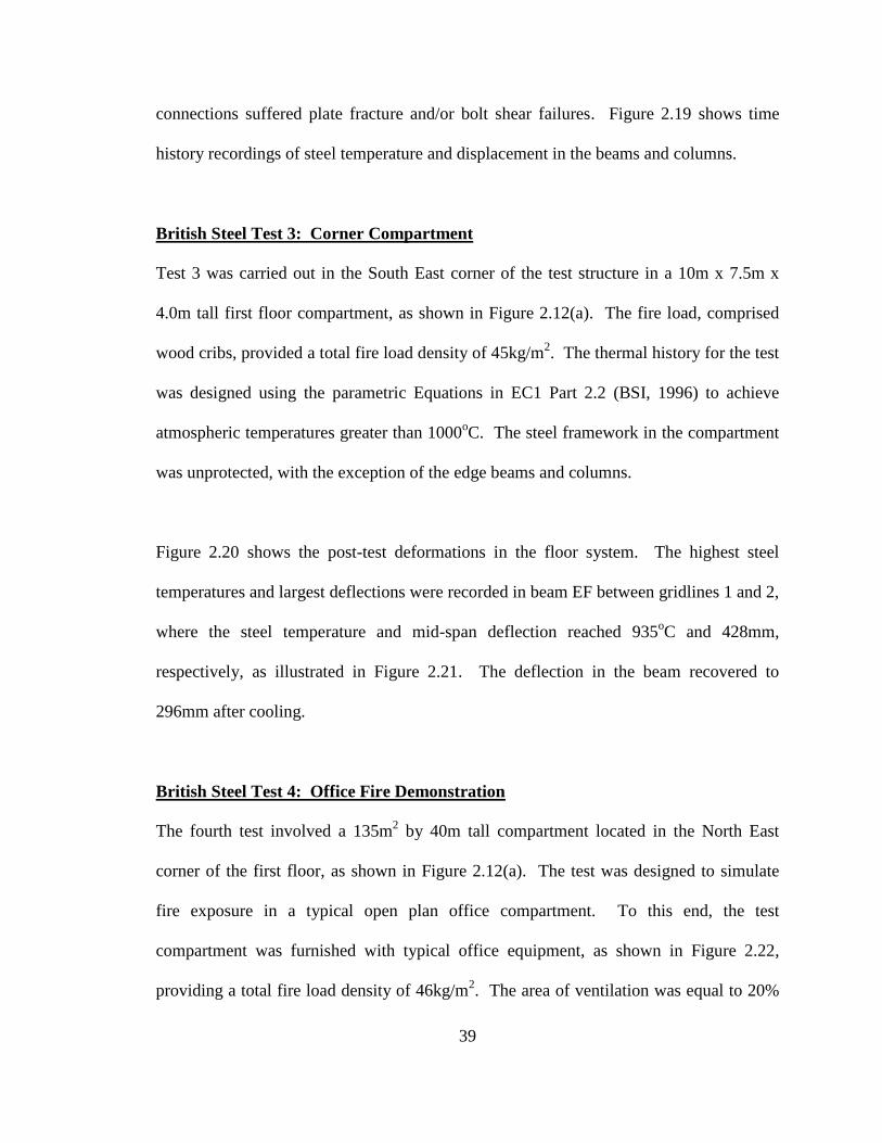
39
connections suffered plate fracture and/or bolt shear failures. Figure 2.19 shows time
history recordings of steel temperature and displacement in the beams and columns.
British Steel Test 3: Corner Compartment
Test 3 was carried out in the South East corner of the test structure in a 10m x 7.5m x
4.0m tall first floor compartment, as shown in Figure 2.12(a). The fire load, comprised
wood cribs, provided a total fire load density of 45kg/m2. The thermal history for the test
was designed using the parametric Equations in EC1 Part 2.2 (BSI, 1996) to achieve
atmospheric temperatures greater than 1000oC. The steel framework in the compartment
was unprotected, with the exception of the edge beams and columns.
Figure 2.20 shows the post-test deformations in the floor system. The highest steel
temperatures and largest deflections were recorded in beam EF between gridlines 1 and 2,
where the steel temperature and mid-span deflection reached 935oC and 428mm,
respectively, as illustrated in Figure 2.21. The deflection in the beam recovered to
296mm after cooling.
British Steel Test 4: Office Fire Demonstration
The fourth test involved a 135m2 by 40m tall compartment located in the North East
corner of the first floor, as shown in Figure 2.12(a). The test was designed to simulate
fire exposure in a typical open plan office compartment. To this end, the test
compartment was furnished with typical office equipment, as shown in Figure 2.22,
providing a total fire load density of 46kg/m2. The area of ventilation was equal to 20%

40
of the floor area. Within the compartment, the columns and beam-column connections
were protected using 25mm ceramic fiber blanket. Both the primary and secondary
beams remained totally exposed, including all beam-to-beam connections.
Steel temperatures in the unprotected beams reached 1150oC (as shown in Figure 2.23),
resulting in maximum deflections of 640mm. As in other tests, extensive buckling was
observed in the beam end regions due to restrained thermal expansion, which resulted in
considerable tensile force demands in the connection regions during the cooling phase of
the fire.
BRE Test 1: Corner Compartment
The BRE corner test was conducted on a 54m2 area along the 2
nd floor of the test
structure, as shown in Figure 2.13(b). The internal compartment boundaries were steel
stud fire resistant board partitions with a fire resistance rating at 2hr. All structural steel
framework, excluding the columns, was left unprotected, and twelve timber cribs were
utilized to provide a fire load of 40kg/m2. At the start of the test, all of the windows and
doors were closed, and the resulting fires were strongly influenced by the lack of oxygen.
It is noted that the fire brigade intervened twice by breaking windows in order to increase
the oxygen supply for the fire.
Atmospheric temperatures of 1051oC were recorded after 102 minutes. The temperature-
time history of the fire atmosphere is shown in Figure 2.24. The bottom flange of the
central secondary beam achieved a maximum temperature of 903oC after 114 minutes,

41
and the maximum recorded slab deflection of 269mm occurred after 130min, which
recovered to 160mm after cooling. The compartment wall performed well and
maintained its integrity through the duration of the test.
BRE Test 2: Large Compartment
The large compartment test was conducted on the second floor (as shown in Figure
2.13(b)), extending over the full width of the building between gridline A and 0.5m from
gridline C. An internal view of the compartment is shown in Figure 2.25. The total floor
area for the compartment was 340m2. Forty-two wooden cribs were used to provide a
fire load of 40kg/m2. The compartment was formed by constructing a fire resistant stud
partition wall across the width of the building and around the vertical access shafts.
Double-glazing was installed on two sides of the building along gridelines 1 and 4. The
middle third of the glazing was left open on both sides to allow sufficient ventilation for
the fire to develop. All steel beams, including the edge beams, were left unprotected.
The columns were protected up to and including the connection regions.
The rapid ignition of the fire caused many of the windows to break during the early part
of the test. This allowed much of the heat generated by the fire to escape through the
window openings and, as a result, kept atmospheric temperatures within the fire
compartment relatively low (763oC). Time history recordings of maximum and average
atmospheric temperature are shown in Figure 2.26. The peak steel temperature of 691oC
and peak vertical displacement of 557mm were recorded halfway between gridlines 2 to
3, and B to C. The maximum residual displacement in the structure was 481mm. Overall

42
the structure behaved very well and there were no signs of collapse. Many of the internal
beams, however, had residual buckling distortions in the lower flange and the web
regions near the connections. Fractures were noted in the end-plate connections, which
were attributed to tensile forces developed during the cooling phase of the fire. It was
also noted that the deflection of the slab caused integrity failure of the compartment wall.
2.4 STRUCTURAL DESIGN FOR FIRE SAFETY
The following section provides a brief overview of conventional building code provisions
for fire safety, including design methodology, component fire tests, and active and
passive fire protection systems.
2.4.1 Design Methodology
The behavior of structures during fire exposure can be markedly different than the
response at normal temperature conditions, and the following considerations need to be
included in the design process:
Material properties of the structural components may be severely degraded at
elevated temperatures.
Internal restraint of thermal expansion may induce significant forces and
deformations in the structural system, irrespective of the external force system.
Temperature-induced material degradation and thermal distortion may increase
vulnerability to failure mechanisms that are generally not considered in a

43
conventional design process, e.g. connection failure due to tensile force demands
during the cooling phase of a fire.
Existing building codes, such as the International Building Code (ICC, 2006), generally
simplify the design approach for fire safety by enforcing prescriptive measures for
building construction (active and passive protection systems), which are largely based on
empirical data and component test results. This prescriptive approach is in stark contrast
to a performance-based engineering approach that addresses the threat and response
characteristics of the structure on a case-by-case basis.
The general design approach for fire safety is illustrated schematically in Figure 2.27,
which was developed by the National Fire Protection Agency (NFPA, 1997). The
primary objectives of the design approach are: (1) to prevent ignition, and (2) to manage
and control a fire that does develop in order to ensure life safety. The first objective is
generally accomplished through restrictions on the use and storage of combustible
material within a structure in order to eliminate environmental conditions that may
promote thermal ignition. The second objective generally requires a combination of
active suppression systems, e.g. automated sprinkler systems, and passive measures (e.g.
thermal insulation) to improve the resilience of the structural system during fire exposure
(collapse prevention), and to ensure a safe means of egress for the occupants (life safety).
To this end, building elements or protection schemes are selected to provide a
prescriptive level of performance, generally measured in the time domain. Newman et al.

44
(2000) provides the following recommendations to improve building performance during
fire exposure:
Compartmentation - Compartment walls should be located on column grid lines
whenever possible. When walls are located off the column grid, large deflections of
unprotected beams can compromise integrity by displacing or cracking the walls
through which they pass. In such cases, the beams should either be protected or
sufficient movement allowance provided. It is recommended that a deflection
allowance of span/30 should be provided in walls crossing the middle half of an
unprotected beam.
Columns - The design guidance is devised to confine structural damage and fire
spread to the fire compartment itself. In order to achieve this, columns should be
designed or protected for the required duration of fire resistance. In buildings of
more than two stories, the applied fire protection should extend over the full height of
the column, including the connection zone. This will ensure that no local squashing
of the column occurs and that structural damage is confined to one floor.
Floor slabs and beams - Floor spans should be limited to a maximum dimension of
9m to prevent excessive deflections during temperature-induced large displacement
response, and the floor slab should be reinforced to develop tensile membrane forces.
2.4.2 Fire Tests
The passive fire resistance of building elements is generally determined through
component fire testing. In the United States, the governing test protocol is provided in

45
ASTM E119 (ASTM, 2000a). The ASTM E119 procedure is a standardized furnace test
that subjects the building component to the temperature history shown in Figure 2.28.
The element is assigned a unique fire rating based on the time required to reach a limiting
failure criterion, which is generally related to deflection or temperature propagation
depending on the function of the element. In this approach, construction methods and
proprietary building elements are prequalified for building applications based on their
published fire rating.
2.4.3 Active Protection Systems
One of the most common active fire suppression systems for building applications is the
automated sprinkler system. Heat sensors are generally used to monitor local
environmental conditions within a compartment. When the sensors record an
atmospheric temperature above a threshold value, indicating the probability of a fire, the
sprinklers are engaged to cool (and therefore retard) the combustion process. Sprinkler
systems are effective in both extinguishing small fires and containing larger fires.
Alarm systems and fire-fighter intervention also fall under the heading of active fire
protection systems. Heat and smoke monitors are effective in notifying occupants and
emergency response personal in the early stages of fire development.
2.4.4 Passive Protection Systems
As previously discussed, the mechanical properties of structural steel are severely
degraded by elevated temperatures. As a result, passive (or non-feedback-based)
46
protection systems are generally needed to enhance the fire performance of steel-framed
buildings, in order to meet the prescriptive fire resistance requirements for the building
design. Passive protection for steel framework generally involves encasing, or insulating,
steel elements with a material that has low thermal conductivity, which effectively
reduces steel temperatures during ambient heating. Common insulation systems include
concrete encasement, heat-resistant board systems, spray-applied fire-resistive insulation,
and intumescent paint.
Due to its relative ease of application (and therefore low cost of installation), spray-
applied fire-resistive material (SFRM) is one of the most widely used forms of thermal
insulation for steel frame building systems. Figure 2.29 presents a typical steel frame
building system protected with SFRM insulation. SFRM is generally cement-based with
some form of glass or cellulosic fibrous reinforcing to hold the material together. Test
methods are available for evaluating the cohesion and adhesion strength of the material
(ASTM, 2000b). The required thickness of proprietary formulations is generally found in
literature published by individual manufacturers.
2.5 SEISMIC PERFORMANCE OF SPRAY-APPLIED FIRE-RESISTIVE
INSULATION
Experimental studies by Braxtan and Pessiki (2009, 2011a, 2011b) demonstrated that
SFRM insulation in moment-frame beam hinge regions is vulnerable to debonding,
cracking, and spalling during inelastic seismic response. The study found that surface
preparation for structural steel has a significant effect on the adhesive bond between the

47
insulation and the steel substrate, as illustrated in Figure 2.30. When mill scale is present
at the time of SFRM application, the bond strength degrades rapidly as strain demands in
the base steel approach yield. This can be attributed to the SFRM bonding to the
sacrificial mill scale and not to the underlying base steel. The consequence of this
unintended interaction is that as the mill scale separates from the steel section, it
contributes to localized debonding of the protective SFRM insulation.
In moment-frame beam hinge regions, earthquake-induced inelastic buckling distortions
can dislodge the delaminated SFRM, leaving exposed surfaces on the structural
framework. Figure 2.31 presents the observed damage to a protected moment-frame
beam-column subassemblage that was subjected to the cyclic displacement-controlled
loading protocol of FEMA 461 (FEMA, 2007). The specimen was insulated with
proprietary 2-hour fire-rated, dry-mix, wool fiber-reinforced SFRM. The insulation spall
along the bottom flange in the beam hinge region, which occurred during an interstory
drift demand of approximately 3%, extends over a length equal to 75% of the beam
depth. Significant cracking and debonding of the SFRM insulation were also noted along
the upper flange and web in the beam hinge region. A similar test utilizing a proprietary
formulation of wet-mix SFRM produced comparable damage. The reader is referred to
Braxtan and Pessiki (2009, 2011a, 2011b) for additional details.

48
2.6 POST-EARTHQUAKE FIRE HAZARD
2.6.1 Introduction
In recent years, post-earthquake fire exposure has drawn attention as a multi-hazard
consideration for building systems. In the aftermath of a major seismic event, spilled fuel,
ruptured gas lines, and damaged electrical equipment can promote thermal ignition. In
addition, impaired active fire suppression mechanisms (e.g. failure of an automatic
sprinkler system due a ruptured water supply line), delayed response time for firefighting
personnel, and damage to thermal barriers (fire walls) increase the likelihood of
uncontrolled fire development and amplify demand on the passive fire resistance of the
building system. Residual damage to structural components and passive fire protection
systems, e.g. earthquake-induced SFRM damage observed by Braxtan and Pessiki
(2011b), can therefore significantly impact building performance during post-earthquake
fire exposure.
2.6.2 Case Studies
Records of post-earthquake fire damage from several large magnitude seismic events
illustrate the significance of the multi-hazard scenario. Fire loss following the 1906
earthquake in San Francisco, California was estimated to be roughly ten times greater
than loss associated with the ground shaking alone, although it has been contended that
many of these fires were manually ignited to falsify insurance claims. In the aftermath of
the 1923 Tokyo Earthquake in Japan, an estimated three quarters of the lost buildings and
56,000 deaths were attributed to post-earthquake building fires. Damage estimates for
more recent seismic events, such as the 1994 Northridge Earthquake in southern

49
California and the 1995 Great Hanshin Earthquake in Kobe, Japan, range into the tens to
hundreds of billions of US dollars (Scawthorn, 2008). Faggiano (2007) reports that
nearly 7000 buildings in Kobe were destroyed by post-earthquake fires alone.
2.6.3 Assessment of the Post-Earthquake Fire Hazard
A critical aspect of assessing structural vulnerability for the post-earthquake fire hazard
involves estimating fire exposure (number of ignitions) and severity (fire-related loss)
following a given seismic event. The following provides a brief summary of relevant
studies on post-earthquake fire modeling.
Cousins and Smith (2004) used historical data from earthquakes in three New
Zealand cities to develop a probabilistic model for estimating loss due to post-
earthquake fire, and to characterize the relative impact of post-earthquake fire on total
loss for a given event.
Ren and Xie (2004) used historical data to develop a probabilistic model for post-
earthquake fire ignition, and linked the algorithm to a geographical information
system (GIS) in order to provide emergency response personal with a simulation tool
for predicting post-earthquake fire spread.
Scawthorn (2008) used a probabilistic model to estimate potential fire loss arising
from a hypothetical M7.8 earthquake in southern California. In the scenario,
approximately 1,600 ignitions would occur that would require intervention of fire-
fighting personnel. In roughly, 1,200 of these fires, the first responding engine would
not be able to adequately contain the fire, which would ultimately spread to adjacent

50
buildings and potentially destroy several city blocks. The estimated loss would range
from 40-100 billion US dollars.
Lee and Davidson (2008) developed a physics-based approach for modeling post-
earthquake fire spread that considers (1) evolution of fire within a room; (2) room-to-
room spread within a building, and (3) building-to-building spread by flame
impingement and radiation from window flames and branding.
Kelly and Tell (2011) proposed a statistical model for predicting the number of fire
ignitions following an earthquake based on historical data for earthquakes from 1906
to 1989 in Alaska and California.
2.6.4 Assessment of Building Performance during Post-Earthquake Fire Exposure
Research on post-earthquake building response during fire exposure is very limited. The
following presents a brief review of several relevant analytical studies.
Corte et al. (2003) analyzed the post-earthquake fire-resistance of single-bay, single-
story and single-bay, multi-story steel moment-frames using assumed temperature-
adjusted resistance functions for unprotected structural elements. Residual
earthquake-induced damage in the system was idealized by considering various initial
displaced shapes for the test specimens. The study determined that response of the
structural system during fire exposure was influenced by the presence of destabilizing
forces in the system, which could drive lateral drift demands during ambient thermal
heating.
Faggiano et al. (2007) utilized sequentially coupled heat transfer-stress analyses to
evaluate the effect of residual destabilizing forces on the response of an unprotected

51
steel portal frame during fire exposure. Nonlinear dynamic response history analyses
were used to characterize peak and residual drift demands in the frame for various
levels of seismic intensity. A thermo-mechanical post-earthquake fire model was
then built in the deformed configuration to evaluate the effect of second-order
destabilizing gravity loads. The study found that a sidesway collapse mechanism
could be developed in the frame for cases with low residual stability indices, i.e. large
ratio of second-order destabilizing gravity load to elastic restoring force.
Yassin et al. (2008) investigated the post-earthquake fire-resistance of single-bay,
single-story and single-bay, two-story steel moment-frames using the nonlinear finite
element software SAFIR (Fransen et al., 2000). The residual destabilizing forces in
the damaged building were modeled with an idealized lateral load pattern that was
scaled to various levels of intensity. Thermal insulation for the frames was assumed
to be damaged during dynamic response, and was therefore neglected from the
component heat transfer analyses, i.e. the heat transfer analyses were performed using
the bare steel sections. Ambient fire exposure for the simulation utilized the
temperature history from the ASTM E119 (ASTM, 2000) standard fire curve. The
study found that residual second-order destabilizing forces in the damaged building
could exacerbate lateral drift demands in the frames during ambient thermal heating.
2.7 SUMMARY
Relevant background material for the study was presented in this Chapter, including an
overview of compartment fire behavior and heat transfer mechanisms, a discussion
regarding the response of steel frame building systems at elevated temperatures, a review

52
of the conventional design approach for fire safety, and a summary of previous research
related to the post-earthquake fire hazard.
A recent study by Braxtan and Pessiki (2009, 2011a, 2011b) on the seismic performance
of spray-applied fire-resistive insulation was discussed. The experimental results indicate
that spray-applied fire-resistive insulation in moment-frame beam hinge regions is
vulnerable to cracking, debonding, and spalling during seismic response, which can
expose regions of bare steel to elevated ambient temperatures during a post-earthquake
fire. This poses a potential threat for steel moment-frame buildings, considering that
temperature-induced softening of the beam hinge regions may increases vulnerability for
local and/or global instabilities.
Historical accounts of post-earthquake fire damage illustrate the significance of the multi-
hazard scenario, and suggest that the probability of fire exposure is greatly increased by a
major seismic event. In addition, the structural and architectural damage caused by
seismic excitation may severely degrade the building’s inherent fire resistance.

53
Table 2.1 Emissivity of structural steel
Reference Emissivity
Eurocode 3 (BSI, 2001) 0.6
(Wang, 2002) 0.7
(Lie, 1992) 0.9
(Holman, 2010) 0.8 (oxidized)
(Lamont et al., 2001) 0.7
(Bejan, 1993) 0.79
0.3 (polished)
0.81 (oxidized)
0.3 (polished)
0.8 (oxidized)
(Siegel and Howell, 1980)
(Brewster, 1992)

54
Figure 2.1 Heat transfer mechanisms during fire exposure (from Lee et al., 2006).
Figure 2.2 Geometric view factor for radiative heat transfer (from Drysdale, 1998).

55
Figure 2.3 EC3 temperature-dependent model for thermal
conductivity of structural steel (BSI, 2001).
Figure 2.4 EC3 temperature-dependent model for
specific heat of structural steel (BSI, 2001).

56
(a)
(b)
Figure 2.5 Micromechanics of structural steel: (a) propagation of edge dislocation
in the crystal grain structure; (b) plastic distortion of the crystal grain structure (adapted from ESA, 2011).

57
Figure 2.6 Experimental measurements of uniaxial stress-strain response
for ASTM A36 steel at elevated temperatures (from NFPA, 1988).
Figure 2.7 EC3 temperature-dependent models for
elastic modulus and yield stress (BSI, 2001).

58
Figure 2.8 Creep strain model for structural steel
at elevated temperature (from Wang, 2002).
Figure 2.9 Poisson’s ratio for structural steel
as a function of temperature (from NIST, 2005).

59
Figure 2.10 Buckled column following the Broadgate
Phase 8 fire, London, UK (from British Steel, 1999).
Figure 2.11 Glazing damage following the Churchill Plaza
fire, Basingstoke, UK (from British Steel, 1999).

60
Figure 2.12 Eight-story steel frame test structure;
Cardington fire tests (from British Steel, 1999).

61
(a)
(b)
Figure 2.13 Fire test locations: (a) British Steel; (b) BRE;
Cardington fire tests (from Lamont, 2001).

62
Figure 2.14 British Steel Test 1 (restrained beam):
test assembly; Cardington fire tests (from British Steel, 1999).
Figure 2.15 British Steel Test 1 (restrained beam):
steel temperature and deflection recordings;
Cardington fire tests (from British Steel, 1999).

63
(a)
(b)
Figure 2.16 British Steel Test 1 (restrained beam): (a) buckled flange
and web elements near the beam ends; (b) fractured beam-column
connection; Cardington fire tests (from British Steel, 1999).

64
Figure 2.17 British Steel Test 2 (plane frame): test assembly;
Cardington fire tests (from British Steel, 1999).
Figure 2.18 British Steel Test 2 (plane frame): residual deformations;
Cardington fire tests (from Lamont, 2001).

65
(a)
(b)
Figure 2.19 British Steel Test 2 (plane frame): steel temperature
and displacement recordings: (a) beam and (b) column;
Cardington fire tests (from British Steel, 1999).

66
Figure 2.20 British Steel Test 3 (corner compartment): residual deformations;
Cardington fire tests (from British Steel, 1999).
Figure 2.21 British Steel Test 3 (corner compartment): steel
temperature and displacement recordings in a secondary beam;
Cardington fire tests (from British Steel, 1999).

67
(a)
(b)
Figure 2.22 British Steel Test 4 (office fire demonstration):
(a) schematic layout; (b) internal view of the compartment;
Cardington fire tests (from British Steel, 1999).

68
Figure 2.23 British Steel Test 4 (office fire demonstration):
ambient temperature at 1.2m below the steel deck;
Cardington fire tests (from British Steel, 1999).
Figure 2.24 BRE Test 1 (corner compartment):
atmospheric temperature recordings;
Cardington fire tests (from British Steel, 1999).

69
Figure 2.25 BRE Test 2 (large compartment):
internal view of the fire compartment;
Cardington fire tests (from British Steel, 1999).
Figure 2.26 BRE Test 2 (large compartment):
atmospheric temperature recordings;
Cardington fire tests (from British Steel, 1999).

70
Figure 2.27 NFPA fire safety concepts tree (from NFPA, 1997).

71
Figure 2.28 ASTM E119 standard fire curve (from ASTM, 2000a).
Figure 2.29 Spray-applied fire-resistive insulation (from Braxtan, 2009).

72
(a)
(b)
Figure 2.30 ASTM E736-00 tensile plate bond tests: (a) test assembly;
(b) SFM-to-steel adhesion strength vs. tensile strain demand
(adapted from Braxtan and Pessiki, 2011a).
WM-M = Wet-mix SFRM; w/ mill-scale WM-SB = Wet-mix SFRM; sandblasted DM-M = Dry-mix SFRM; w/ mill-scale DM-SB = Dry-mix SFRM; sandblasted

73
(a)
(b)
Figure 2.31 FEMA 461 beam-column subassemblage test from Braxtan (2009):
(a) test assembly; (b) observed damage to SFRM insulation.

74
CHAPTER 3
ANALYSIS AND DESIGN OF THE TEN-STORY
STEEL MOMENT-FRAME TEST STRUCTURE
3.1 OVERVIEW
One of the primary objectives of this study was to evaluate the adequacy of current U.S.
building code provisions for preventing sidesway collapse during post-earthquake fire
exposure. The design of the test structure was therefore an integral aspect of the research
program and, as such, an overview of the design process is provided in this chapter. A
complete set of design calculations for the test structure is provided in Keller and Pessiki
(2011a). The goal of this task was to develop a test structure using conventional methods
that would be representative of a typical steel moment-frame office building located near
coastal California.
The design standards referenced for the project are presented in Section 3.2. Building
layout and classification are discussed in Section 3.3. Gravity load demands are
presented in Section 3.4, and the design-basis seismic and wind hazards are discussed in
Sections 3.5 and 3.6, respectively. Design considerations and performance ratings for the
special moment-frames are presented in Section 3.7. Section 3.8 presents the design
approach for fire safety.

75
3.2 DESIGN STANDARDS
The following design standards were referenced in the development of the test structure.
Where applicable, the Load and Resistance Factor Design methodology (LRFD) was
utilized.
2010 California Building Code (CBSC, 2010)
IBC-06: 2006 International Building Code (ICC, 2006)
ASCE/SEI 7-05: Minimum Design Loads for Buildings and Other Structures
(ASCE, 2005)
ANSI/AISC 360-05: Specification for Structural Steel Buildings (AISC, 2005c)
ANSI/AISC 341-05: Seismic Provisions for Structural Steel Buildings
(AISC, 2005a)
ANSI/AISC 358-05: Prequalified Connections for Special and Intermediate Steel
Moment Frames for Seismic Applications (AISC, 2005b)
3.3 BUILDING LAYOUT AND CLASSIFICATION
The test structure is representative of a ten-story steel moment-frame office building
located near coastal California. The typical floor plan and N-S elevation are presented
Figure 3.1. The structure has five-bays in the N-S direction with a typical bay length of
8.5m. In the E-W direction, the structure is seven-bays long with a typical bay length of
8.5m and a center bay length of 9.8m. The height of the first above grade story is 4.5m,
measured from top of slab-to-top of slab. Above the first elevated floor, the typical story
height is 4.1m. The height-to-least width ratio for the structure is 1.0.

76
Lateral force resistance is provided by perimeter special moment-frames (SMF) utilizing
welded unreinforced flange – welded web (WUF-W) beam-column connections. A
schematic elevation for the typical N-S SMF is presented in Figure 3.2, and the
ANSI/AISC 358-05 prequalified WUF-W beam-column connection detail is shown in
Figure 3.3. For constructability and design efficiency, the moment-frame and gravity-
frame columns were spliced every two stories at 1.2m above the finished floor, in
accordance with ANSI/AISC 360-05. A992 steel (ASTM, 2011) was assumed for all
structural elements of the SMF.
The test structure is classified as Business Group B in accordance with IBC-06 Section
304, and utilizes Type 1B non-combustible construction material in accordance with
IBC-06 Section 602. Since the height of the tallest occupied floor is located more than
23m from the lowest level of fire department access, the test structure qualifies as a high-
rise structure and is subject to the additional design requirements of IBC-06 Section 403
(discussed further in Section 3.8 of this dissertation).
3.4 GRAVITY LOADS
The following section presents the gravity loads assumed in the design process. Dead
load demands for the floor system (not including the self-weight of steel) considered the
following components:
Concrete slab over metal deck (100mm total depth): 2kPa
Ceiling: 140Pa
Mechanical/Electrical/Plumbing: 140Pa

77
Floor Covering: 50Pa
Partitions: 960Pa
A floor live load demand of 3800Pa was assumed for design purposes based on the
guidelines of ASCE/SEI 7-05. The weight of the exterior wall system was taken as
480Pa.
3.5 DESIGN-BASIS SEISMIC HAZARD
Seismic analysis of the test structure for the design-basis earthquake (DBE) was in
accordance with the guidelines of IBC-06 and ASCE/SEI 7-05. The following section
provides an overview of the DBE hazard and the procedure utilized to estimate force
demands in the test structure.
3.5.1 Design-Basis Earthquake
IBC-06 and ASCE/SEI 7-05 define the seismic hazard for a structure in terms of an
associated pseudo-acceleration response spectrum, where pseudo-acceleration (or spectral
acceleration) demand is defined in Equation 3-1.
(Equation 3-1)
Where
is the spectral acceleration demand for ground shaking calculated at period T
is the peak displacement demand for ground shaking calculated at period T
is the natural frequency of vibration for the dynamic system equal to

78
In order to facilitate a practical approach for seismic design, ASCE/SEI 7-05 provides
geographically mapped values of prescribed spectral acceleration demand for the
maximum considered earthquake (MCE) at periods of 0.2-second (short period) and 1-
second, designated as and , respectively. These mapped values assume an inherent
damping ratio ( ) of 5% and a Site Class, as defined in IBC-06 Section 1613.5.2, of type
B (rock). For design purposes, the short ( ) and 1-second period ( ) MCE spectral
acceleration demands for the test structure were taken as 1.50 and 0.60 , respectively,
where is defined as gravitational acceleration.
Site modification factors and from IBC-06 Section 1613.5.2 are then used to adjust
the MCE spectral acceleration demand in the acceleration-controlled and velocity-
controlled response regions, respectively, in order to account for the effect of soil
conditions on ground motion response. For the test structure, site class D (stiff soil)
conditions were assumed, and the site coefficients for the acceleration-controlled ( ) and
velocity-controlled ( ) response regions were taken as 1.0 and 1.5, respectively. The
assumption of site class D conditions is consistent with the ASCE/SEI 7-05
recommendation when soil profiles are not known in sufficient detail. The site adjusted
MCE spectral acceleration demands at short and 1-second periods are presented in
Equations 3-2 and 3-3.
( )( ) (Equation 3-2)
( )( ) (Equation 3-3)

79
Where
is the site-adjusted spectral acceleration demand for MCE ground shaking
calculated at a period of 0.2-second
is the site-adjusted spectral acceleration demand for MCE ground shaking
calculated at a period of 1-second
DBE spectral acceleration demands are then determined, in accordance with IBC-06
Equations 16-39 and 16-40, by scaling the MCE demands by a factor of 2/3, as shown in
Equations 3-4 and 3-5.
( ) ( )( ) (Equation 3-4)
( ) ( )( ) (Equation 3-5)
Finally, a response spectrum for the site, which provides prescribed pseudo-acceleration
demand over a range of vibration periods, is developed for the DBE hazard using the
procedure outlined in ASCE/SEI 7-05 Section 11.4.5. The DBE response spectrum for
the test structure site is presented in Figure 3.4.
3.5.2 ASCE/SEI 7-05 Equivalent Lateral Force Procedure
Once the DBE response spectrum has been developed for the site, peak force and
deformation demands in the structure are estimated using the guidelines of ASCE/SEI
7-05. First, a seismic design category for the structure is determined using IBC-06 Table
1613.5.6, based on the occupancy classification defined in ASCE/SEI 7-05 Table 1-1.
For the test structure, an occupancy classification of II and a seismic design category of D

80
were assumed. The fundamental period of the structure is then estimated in accordance
with ASCE/SEI 7-05 Section 12.8.2.1 as the smaller of: (a) the fundamental period
calculated from eigenvalue analysis; and (b) 1.4 times the approximate period calculated
from Equation 3-6.
(Equation 3-6)
Where
Ta is the approximate fundamental period
Ct and x are parameters related to the lateral force resisting system, taken as 0.028
and 0.8, respectively, for buildings utilizing steel SMF
hn is the building height above grade
For the test structure, the upper limit of controlled, and the fundamental period
was estimated as 2.0-seconds.
An analysis procedure is then selected based on the vibration characteristics of the
structure and the seismic design category. For the test structure, the equivalent lateral
force procedure of ASCE/SEI 7-05 Section 12.8 was selected based on the following
considerations:
Fundamental period less than 3.5 times the ratio between the DBE spectral
acceleration demand at 1-second and 0.2-second ( ).
Regular geometry (as defined in ASCE/SEI 7-05 Section 6.2).
Seismic Design Category D.

81
The equivalent lateral force procedure is a simplified analytical method for earthquake
analysis that uses prescribed response modification factors to adjust results from an
elastic static analysis, in order to account for a presumed level of inelastic behavior.
Graphical representations of the response modification factors in terms of force-
deformation and spectral response parameters are presented in Figures 3.5 and 3.6,
respectively. The response modification factors for the test structure were taken from
ASCE/SEI 7-05 Table 12.2-1 for the steel SMF lateral force resisting system (system
type C1).
The strength modification coefficient ( ) is defined in Equation 3-7 as the ratio of the
seismic base shear demand that would be developed in the system for DBE ground
motions if the system remained entirely linearly elastic ( ), to the base shear
prescribed for design ( ). For a building utilizing a steel SMF lateral force resisting
system, an R value of 8 is assumed.
(Equation 3-7)
The system overstrength factor ( ) is defined in Equation 3-8 as the ratio of the
maximum base shear resistance ( ) to the design base shear ( ). An value
of 3 is assumed for a building utilizing a steel SMF lateral force resisting system
⁄ (Equation 3-8)

82
The deflection amplification factor ( ) is utilized in the design process to estimate peak
lateral deflection demand ( ) for the DBE by adjusting the deflection demand from
a linear elastic analysis ( ), as shown in Equation 3-9. For a building utilizing a
steel SMF lateral force resisting system, a value of 5.5 is assumed.
( )⁄ (Equation 3-9)
In the equivalent lateral force procedure, inertial force demands are estimated with
respect to the effective seismic weight ( ) of the building, which is defined by
ASCE/SEI 7-05 Section 12.7.2 as the total unfactored dead load, including a minimum
partition load of 480Pa, plus probable snow loading. Based on the site location, snow
load demand for the test structure was neglected, and the effective seismic weight was
estimated as 102,000kN.
The DBE seismic base shear demand ( ) for the equivalent lateral force procedure
is then calculated in accordance with ASCE/SEI 7-05 Section 12.8.1.1. This force
demand is commonly presented in terms of a seismic coefficient ( ) for the structure,
defined in Equation 3-10 as the DBE lateral base shear demand ( ) normalized by
the effective seismic weight ( ). The relationship between the seismic coefficient and
spectral acceleration demand is shown graphically in Figure 3.6, where is the MCE
spectral acceleration demand calculated at period . For the test structure, the seismic
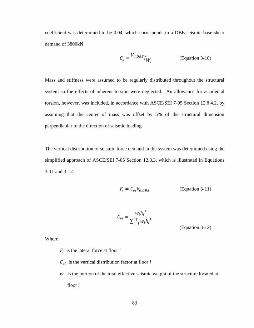
83
coefficient was determined to be 0.04, which corresponds to a DBE seismic base shear
demand of 3800kN.
⁄ (Equation 3-10)
Mass and stiffness were assumed to be regularly distributed throughout the structural
system so the effects of inherent torsion were neglected. An allowance for accidental
torsion, however, was included, in accordance with ASCE/SEI 7-05 Section 12.8.4.2, by
assuming that the center of mass was offset by 5% of the structural dimension
perpendicular to the direction of seismic loading.
The vertical distribution of seismic force demand in the system was determined using the
simplified approach of ASCE/SEI 7-05 Section 12.8.3, which is illustrated in Equations
3-11 and 3-12.
(Equation 3-11)
∑
(Equation 3-12)
Where
is the lateral force at floor i
is the vertical distribution factor at floor i
is the portion of the total effective seismic weight of the structure located at
floor i

84
is the height of floor i above grade
is an exponent related to the structure period, taken as follows:
for structures having a period of 0.5-second or less, k = 1
for structures having a period of 2.5-seconds or more, k = 2
for structures having a period between 0.5 and 2.5 seconds, k shall be 2 or
shall be determined by linear interpolation.
The design-level force demand on the structural system is generally controlled by the
ASCE/SEI 7-05 load case presented in Equation 3-13.
( ) (Equation 3-13)
Where
is the load effect related to dead load demand
is the load effect related to live load demand
is the load effect related to snow load demand (neglected for site)
is the load effect related seismic load demand
is a redundancy factor, taken as 1.0 for regular building configurations
3.6 DESIGN-BASIS WIND HAZARD
The design wind hazard for the site was developed using the guidelines of ASCE/SEI
7-05. Because the test structure was regular-shaped, as defined in ASCE/SEI 7-05
Section 6.2, and did not possess any response characteristics that would make it
susceptible to large-scale wind-induced excitation from extraneously-induced (e.g.

85
buffeting), instability-induced (e.g. vortex shedding), and/or movement-induced (e.g.
galloping) mechanisms, the analytical procedure of ASCE/SEI 7-05 Section 6.5 was
utilized for lateral load analysis.
The design wind speed ( ) was estimated from mapped values as 38m/s, with a wind
directionality factor ( ) of 0.85. The importance factor ( ) for the structure was taken
as 1.00, and a topographic factor ( ) of 1.0 was assumed for the site.
The test structure was classified as flexible in accordance with ASCE/SEI 7-05 Section
6.2 since the fundamental frequency (0.41Hz), as determined from eigenvalue analysis,
was less than 1Hz. The gust effect factor ( ) was therefore calculated using the
rigorous approach of ASCE/SEI 7-05 Section 6.5.8.2 in order to account for potential
dynamic amplification due to movement-induced excitation. A site surface roughness
category of B and an exposure classification of B were assumed for the urban setting.
A partially enclosed building envelope was assumed with an internal pressure coefficient
( ) of + 0.55. The external pressure coefficient ( ) for the main wind-resisting
system was taken as 0.8 for the windward surface and -0.5 for the leeward surface.
The controlling load case for lateral load analysis of the test structure for wind loading is
presented in Equation 3-14.
(Equation 3-14)

86
Where
W is the load effect related to wind load demand
Lr is the load effect related to roof live load demand
3.7 ANALYSIS AND DESIGN OF THE N-S SPECIAL MOMENT-FRAMES
The following section presents the analytical model developed to evaluate lateral load
response of the test structure in the N-S direction, and discusses performance
requirements for ductile steel moment-frames. A summary of design performance ratios
( ) for the test structure N-S SMF is provided in Section 3.7.3, where the performance
ratio index is defined in Equation 3-15.
⁄ (Equation 3-15)
Where
is the response demand
is the response capacity
3.7.1 Lateral Load Response Model
An idealized second-order elastic model for the test structure was developed in the finite
element software Abaqus (Abaqus, 2011) to evaluate the uncoupled unidirectional lateral
load response in the N-S direction. The analytical model, a schematic of which is
presented in Figure 3.7, was composed of two analytical substructures: (1) a SMF
substructure used to model lateral load resistance of the N-S SMF; and (2) a leaning
column substructure used to model second-order destabilizing loading from the tributary

87
building mass. Neglecting torsional modes of response (with the exception of lateral
force amplification to account for accidental torsion, discussed in Section 3.5.2) the
system was idealized as a half-system submodel with a single perimeter SMF and a
leaning column carrying half of the respective floor loads.
The SMF substructure was modeled with cubic-formulation beam-column elements using
centerline dimensions, a conventional approach used to account for flexibility in the
beam-column panel zones. The stiffening effect of composite behavior between the
moment-frame beams and floor slab (away from the designated beam hinge regions) was
conservatively neglected. The column bases were assumed to be fully restrained by the
building foundation (fixed boundary condition). Lateral force demands at the floor levels
(developed in the preceding sections) were evenly distributed as concentrated nodal loads
acting at the beam-column work points.
The leaning column substructure was incorporated to model second-order destabilizing
loads in the system. This was accomplished by activating geometric nonlinearity in the
solution algorithm. It is noted that Abaqus uses a large-displacement approach for
geometric nonlinearity where equilibrium is formulated on the displaced nodal geometry.
Kinematic constraints were used to tie lateral translations at corresponding floor levels in
the SMF and leaning column substructures. Vertical translations and in-plane rotations
were uncoupled between the linked nodes, thereby allowing second-order destabilizing
lateral loads to be included the analysis without overestimating the gravity forces acting
on the SMF substructure. In order to minimize the lateral resistance provided by the

88
leaning column substructure, the support node at the base of the column was pinned (free
to rotate), and a relatively small moment of inertia was assigned to the leaning column
cross-section (1/10th
of the largest moment of inertia for the SMF columns). This
approach conservatively ignored the lateral resistance provided by the gravity-frames.
The cross-sectional area of the leaning column section was assigned a cross-sectional
area equal to the sum of the cross-sectional areas for the tributary gravity columns.
3.7.2 Performance Requirements
The seismic design of steel moment-frames for mid-rise and high-rise buildings is
generally governed by drift control requirements. ASCE/SEI 7-05 Table 12.12-1 limits
the interstory drift demands in the system, measured in terms of the interstory drift ratio
defined in Equation 3-16, to 2% for the DBE.
⁄
(Equation 3-16)
Where
is the interstory drift ratio demand in story i
is the amplified interstory drift demand in story i, equal to the absolute
difference in lateral displacement in the upper and lower floors
is the height of story i
In addition, ASCE/SEI 7-05 Section 12.8.7 requires that the second-order destabilizing
moment demand in each story for the DBE is kept with a specified tolerance, in order to
provide adequate safety for sidesway collapse. This is enforced by maintaining a stability

89
coefficient, defined in Equation 3-17 as the ratio of destabilizing moment demand to
seismic shear force demand in the story, less the prescriptive upper limit provided by
Equation 3-18.
(Equation 3-17)
Where
is the stability coefficient for story i
is the total unfactored vertical load acting on the upper floor in story i
is the seismic shear force in story i
According to ASCE/SEI 7-05, the lateral load analysis must consider second-order
effects if the stability coefficient for any story exceeds 0.10. The structure is considered
potentially unstable if the stability coefficient for any story exceeds the allowable
stability coefficient , determined as:
(Equation 3-18)
Where
is the ratio of shear demand to shear capacity for story i.
Story shear demand is determined from static analysis. Story shear capacity is
approximated as the sum of the probable flexural capacities in the beam hinge regions
along the upper floor, divided by the story height, as defined in Equation 3-19 and shown
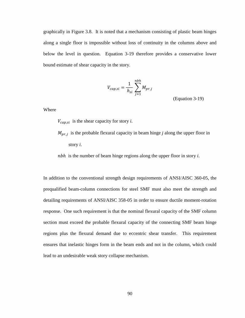
90
graphically in Figure 3.8. It is noted that a mechanism consisting of plastic beam hinges
along a single floor is impossible without loss of continuity in the columns above and
below the level in question. Equation 3-19 therefore provides a conservative lower
bound estimate of shear capacity in the story.
∑
(Equation 3-19)
Where
is the shear capacity for story i.
is the probable flexural capacity in beam hinge j along the upper floor in
story i.
is the number of beam hinge regions along the upper floor in story i.
In addition to the conventional strength design requirements of ANSI/AISC 360-05, the
prequalified beam-column connections for steel SMF must also meet the strength and
detailing requirements of ANSI/AISC 358-05 in order to ensure ductile moment-rotation
response. One such requirement is that the nominal flexural capacity of the SMF column
section must exceed the probable flexural capacity of the connecting SMF beam hinge
regions plus the flexural demand due to eccentric shear transfer. This requirement
ensures that inelastic hinges form in the beam ends and not in the column, which could
lead to an undesirable weak story collapse mechanism.

91
3.7.3 Performance Ratios for the N-S Special Moment-Frames
DBE-level performance ratios for the N-S SMF are presented in Tables 3-1 to 3-5, and
column-beam flexural strength ratios for the beam-column connections are presented in
Table 3-6. As anticipated, the design was driven by drift control requirements for seismic
loading (Table 3-1) and ductility requirements for the prequalified beam-column
connections (Table 3-6). Performance ratios for interstory drift demand ranged from 0.6
to 1.0, with seven of the ten stories exceeding a performance ratio of 0.9. Story stability
performance ratios for the DBE were between 0.11 and 0.58, indicating a considerable
inherent resistance to sidesway instability. Performance ratios for flexural and shear
demands in the SMF beams ranged from 0.30-0.46 and 0.31-0.53, respectively. It is
noted that the flexural demand in the SMF beams due to wind loading was approximately
60-70% of the demand imposed by seismic loading. The critical performance ratio for
combined flexure and axial compression in the moment-frame columns, measured in the
first story, was determined to be 0.6. All five of the beam-column connection
configurations below the roof level had flexural strength ratios less than 1.1.
3.8 DESIGN FOR FIRE SAFETY
Fire protection for the building was achieved through a combination of active suppression
systems (e.g. automatic sprinklers) and augmentation of passive resistance (e.g. spray-
applied fire-resistive insulation) based on the prescriptive guidelines of IBC-06. This
section presents an overview of the active and passive measures utilized to enhance fire
performance of the structural system.

92
3.8.1 Active Fire Protection
Since the test structure qualifies as a high-rise building, as defined in IBC-06 Section
403, all floors were required to be protected with an automatic sprinkler system in
accordance with IBC-06 Section 403.2. In addition, since the primary usage of the
building is for office rental space, the California Building Code requires that the structure
be equipped with a heat and smoke monitoring system capable of relaying information to
emergency response and fire-fighting personnel.
3.8.2 Passive Fire Protection
The construction classification for the building was defined as Type 1B non-combustible
material in accordance with IBC-06 Section 602. For this type of construction, IBC-06
Table 601 requires that the structural components provide a minimum fire resistance (in
the time domain) of 2-hours. In order to meet this requirement, the structural steel
framework was passively protected with a proprietary two-hour fire-rated dry-mix spray-
applied fire-resistive insulation. Details regarding the fire-resistive insulation for the N-S
SMF members are provided in Table 3-7. The product specification and design aid
provided by the manufacturer (Isolatek, 2011) are provided in Appendix 1
.
3.9 SUMMARY
The ten-story steel moment-frame test structure was presented in this chapter, along with
the design-basis loads and analytical assumptions. Conventional analysis methods and
procedures were utilized to develop a representative design for an office building located
near coastal California. The design of the steel special moment-frame lateral force

93
resisting system was driven by drift control requirements for seismic loading and ductility
requirements for the prequalified beam-column connections. Fire protection for the
building was achieved through a combination of active suppression systems (e.g.
automatic sprinklers) and augmentation of passive resistance (e.g. spray-applied fire-
resistive insulation).

94
Table 3.1 Interstory drift performance ratios,
response in the N-S direction
Table 3.2 Story stability performance ratios,
response in the N-S direction
IDR Demand, IDR Capacity, Performance Ratio,
IDRd IDRa PRIDR
(%) (%) (IDRd / IDRa)
1 1.20 2.00 0.60
2 1.70 2.00 0.85
3 1.90 2.00 0.95
4 2.00 2.00 1.00
5 2.00 2.00 1.00
6 1.90 2.00 0.95
7 1.90 2.00 0.95
8 1.80 2.00 0.90
9 1.50 2.00 0.75
10 1.10 2.00 0.55
Story
Performance Ratio,
PRθs
(θs / θs,max)
1 0.110 0.250 0.44
2 0.144 0.250 0.58
3 0.146 0.250 0.58
4 0.140 0.250 0.56
5 0.122 0.250 0.49
6 0.103 0.250 0.41
7 0.093 0.250 0.37
8 0.078 0.250 0.31
9 0.053 0.250 0.21
10 0.027 0.250 0.11
Story Stability
Index, θs
Story
Allowable
Story Stability
Index, θs,max

95
Table 3.3 Beam flexure performance ratios, N-S SMF
Table 3.4 Beam shear performance ratios, N-S SMF
Gravity + Seismic Gravity + Wind
(kN-m) (kN-m) (kN-m) (Mu/ϕMn)
W920x223
(W36x150)1.19E+03 8.44E+02 2.96E+03 0.40
W840x193
(W33x130)1.08E+03 7.15E+02 2.38E+03 0.46
W760x161
(W30x108)7.25E+02 3.99E+02 1.76E+03 0.41
W690x140
(W27x94)4.29E+02 2.50E+02 1.41E+03 0.30
W610x92
(W24x62)2.33E+02 1.71E+02 7.78E+02 0.30
Beam Section
Flexural Demand, Mu Design Flexural
Capacity, ϕMn
Performance
Ratio, PRf
Gravity + Seismic Gravity + Wind
(kN) (kN) (kN) (Vu/ϕVn)
W920x223
(W36x150)1.36E+03 2.67E+02 2.99E+03 0.45
W840x193
(W33x130)2.36E+02 1.35E+03 2.56E+03 0.53
W760x161
(W30x108)8.40E+02 1.60E+02 2.17E+03 0.39
W690x140
(W27x94)6.91E+02 1.25E+02 1.76E+03 0.39
W610x92
(W24x62)4.20E+02 1.07E+02 1.36E+03 0.31
Beam Section
Shear Demand, Vu Design Shear
Capacity, ϕVn
Performance
Ratio, PRv
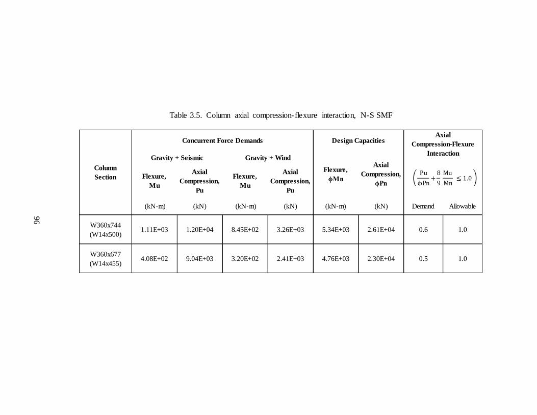
Table 3.5. Column axial compression-flexure interaction, N-S SMF
Flexure,
Mu
Axial
Compression,
Pu
Flexure,
Mu
Axial
Compression,
Pu
(kN-m) (kN) (kN-m) (kN) (kN-m) (kN) Demand Allowable
W360x744
(W14x500)1.11E+03 1.20E+04 8.45E+02 3.26E+03 5.34E+03 2.61E+04 0.6 1.0
W360x677
(W14x455)4.08E+02 9.04E+03 3.20E+02 2.41E+03 4.76E+03 2.30E+04 0.5 1.0
Column
Section
Concurrent Force DemandsAxial
Compression-Flexure
Interaction Gravity + Seismic Gravity + Wind
Design Capacities
Flexure,
ϕMn
Axial
Compression,
ϕPn
96

Table 3.6. Column-beam flexural strength ratios, N-S SMF
Section
Nominal Flexural
Capacity, Reduced by
Axial Force Demand,
Mn,col
SectionProbable Flexural
Capacity, Mpr,bm
(kN-m) (kN-m) (kN-m)
W360x744
(W14x500) 5.35E+03
W920x223
(W36x150) 5.06E+03 3.38E+02 1.0
W360x677
(W14x455) 4.85E+03
W840x193
(W33x130) 4.06E+03 3.27E+02 1.1
W360x592
(W14x398) 4.21E+03
W840x193
(W33x130) 4.06E+03 3.14E+02 1.0
W360x463
(W14x311) 3.21E+03
W760x161
(W30x108) 3.01E+03 1.82E+02 1.0
W360x382
(W14x257) 2.66E+03
W690x140
(W27x94) 2.42E+03 1.44E+02 1.0
W360x382
(W14x257) 2.70E+03
W610x92
(W24x62) 1.33E+03 8.75E+01 1.9
Column BeamFlexural Demand
due to
Eccentric Shear
Transfer, Mv
Column - Beam
Strength Ratio
97

98
Table 3.7 Spray-applied fire-resistive insulation, N-S SMF
Rating
(hr)
UL
Designation
Required
Thickness
(mm)
W920x223 (W36x150)
Beam2 N815 25
W840x193 (W33x130)
Beam2 N815 27
W760x161 (W30x108)
Beam2 N815 29
W690x140 (W27x94)
Beam2 N815 29
W610x92 (W24x62)
Beam2 N815 33
W360x744 (W14x500)
Column2 X829 9.5
W360x677 (W14x455)
Column2 X829 11
W360x592 (W14x398)
Column2 X829 11
W360x463 (W14x311)
Column2 X829 13
W360x382 (W14x257)
Column2 X829 13
Section
Dry Mix SFRM Insulation

99
(a) (b)
Figure 3.1 Ten-story steel moment-frame test structure:
(a) typical floor plan, (b) N-S elevation.
(a) (b)
Figure 3.2 Typical N-S special moment-frame:
(a) U.S. customary sections, (b) metric sections.

100
Figure 3.3 Welded unreinforced flange – welded web (WUF-W)
beam-column connection (from ANSI/AISC, 2005b).
Figure 3.4 Response spectrum for the design-basis earthquake (DBE).

101
Figure 3.5 Response modification factors for the equivalent lateral force
procedure in terms of force-deformation parameters.
Figure 3.6 Response modification factors for the equivalent lateral
force procedure in terms of spectral parameters.

102
Figure 3.7 Second-order elastic lateral load response model.
Figure 3.8 Beam-column sidesway mechanism (from Charney, 2010).

103
CHAPTER 4
NONLINEAR MULTI-DEGREE-OF-FREEDOM
DYNAMIC RESPONSE MODEL
4.1 OVERVIEW
This section describes the nonlinear multi-degree-of-freedom (MDOF) dynamic response
model developed for the ten-story steel special moment-frame (SMF) test structure,
which was discussed in Chapter 3. The numerical time-stepping algorithm for the
nonlinear dynamic simulation is discussed in Section 4.2. Section 4.3 provides an
overview of the analytical components and global connectivity. The special moment-
frame and leaning column substructures are discussed in Sections 4.4 and 4.5,
respectively. Section 4.6 presents the equivalent viscous damping model for inherent
(non-simulated) energy-dissipation mechanisms in the structural system. Gravity and
seismic force demands are discussed in Section 4.7. Sample batch files for executing the
simulation in OpenSees (OpenSees, 2011), an analytical framework for nonlinear finite
element analysis, can be found in Keller and Pessiki (2011a). The files are applicable to
v2.2.2 of the source code.
4.2 NUMERICAL TIME-STEPPING PROCEDURE
The implicit Newmark two-parameter time-stepping procedure, assuming average
acceleration over the time step (γ = 1/2 and β = 1/4), was utilized to simulate nonlinear
dynamic response of the test structure for earthquake excitation. An overview of the
numerical procedure is presented in Appendix 2.

104
For the dynamic response history analyses of Chapter 6, the convergence tolerance
(discussed in Appendix 1) was set to 1E-10, based on recommendations in the OpenSees
documentation, and the maximum number of Newton-Raphson iterations was set to 9000.
It is noted that the upper limit on Newton-Raphson iterations is somewhat arbitrary, but
should be large enough to promote numerical convergence.
4.3 ANALYTICAL COMPONENTS AND GLOBAL CONNECTIVITY
An idealized analytical model for the test structure was developed in the nonlinear finite
element software OpenSees to study unidirectional seismic excitation in the N-S
direction. A schematic detail of the model is presented in Figure 4.1. Neglecting out-of-
plane and torsional modes of response, the structural system was idealized as a half-
system submodel composed of three integrated analytical components: (1) a nonlinear
special moment-frame (SMF) substructure used to model the lateral load resistance
provided by a typical N-S SMF; (2) a leaning column substructure used to model the
tributary building mass, including second-order P-delta effects; and (3) a network of
equivalent viscous damping substructures used to model inherent (non-simulated)
energy-dissipation mechanisms in the structural system, e.g. hysteretic stress-strain
response in architectural features and internal friction. Multi-point kinematic constraints
were used to slave lateral translations in the SMF and damping substructures to the
dynamic degrees-of-freedom in the leaning column substructure, thereby engaging the
lateral force resisting system and viscous dashpots (inherent damping model) during
dynamic excitation. Vertical translations and in-plane rotations were uncoupled between

105
the linked nodes, primarily to ensure that gravity load demand on the SMF substructure
was not overestimated.
4.4 SPECIAL MOMENT-FRAME SUBSTRUCTURE
4.4.1 Overview
The SMF substructure was developed to model the lateral load resistance provided by a
typical N-S SMF, and considered inelastic response in the beam-column connection and
column base regions. Outside of these locations, beam and column sections were
modeled with conventional linear elastic cubic formulation beam-column elements. For
consistency with the design assumptions, the column supports were modeled as fully
restrained (fixed) boundary conditions.
A schematic of the nonlinear beam-column connection model for the SMF substructure is
presented in Figure 4.2. Potential inelastic hinge regions in the beam and column ends on
either side of the panel zone were modeled with nonlinear fiber elements, and a flexible
panel zone model was developed to account for web plate shear deformation and column
flange flexure. The inelastic beam hinge and panel zone models are discussed further in
Sections 4.3.2 and 4.3.3, respectively.
4.4.2 Fiber Element Hinge Model
4.4.2.1 Overview
Potential locations of inelastic hinging in the SMF substructure, including the beam and
column end regions on either side of the beam-column connection panel zone, and the

106
column base regions, were modeled with force-based (or flexibility-based) fiber beam-
column elements. The methodology for the fiber element model is shown schematically
in Figure 4.2. State determination calculations during the analysis are performed at
specified section integration points along the fiber element length. At the section
integration points, the member cross-section is discretized in two-dimensional space into
a number of longitudinal fibers, where each of these fibers has associated geometric
properties, e.g. cross-sectional area and distance from the local centroidal axis of the fiber
to the reference (or bending) axis for the section, and associated material properties, e.g.
uniaxial stress-strain response model. Integration of the tangent mechanical properties
for the fibers yields the tangent mechanical stiffness matrix for the slice section. For the
case of a fiber beam-column element subject to biaxial bending and axial extension, the
fiber-section stiffness relation is expressed in Equation 4-21.
( )
[
∑
( )
∑
( )
∑
( )
∑
( )
∑
( )
∑
( )
∑
( )
∑
( )
∑
( )
]
(Equation 4-1)
Where
( ) is the tangent section stiffness matrix at the jth
element iteration
is the tangent modulus of fiber i at the jth
element iteration

107
is the cross-sectional area of fiber i
and define the distance from the centroidal axis of fiber i to the
reference axis for the section
( ) designates the number of fibers in the section at location x along the member
length
The fiber element approach accounts rationally for nonlinear inelastic axial-flexural
interaction and distributed plasticity. In contrast to a “lumped plasticity” model where
inelastic behavior is concentrated in zero-length plastic hinges, the fiber element hinge
model considers the spread of inelastic behavior both across the section and along the
member length. The fiber element hinge model, however, does have several notable
limitations: (1) it is unable to explicitly model geometric softening due to local flange
and web buckling; (2) it idealizes stress-strain response in the cross-section as uniaxial,
which could misrepresent stress demands in regions where end restraint is significant,
e.g. near the beam-column flange interface where the stress field is triaxial; and (3) shear
deformations are generally uncoupled from axial-flexural response, which could be
significant for sections where flexural-shear interaction is significant.
The fiber element approach to nonlinear structural analysis is discussed in Zeris and
Mahin (1988, 1991), Taucer et al. (1991), Spacone et al. (1992), and Neuenhofer et al.
(1997, 1998). The advantage of the force-based (or flexibility-based) element
formulation, as opposed to the displacement-based (or stiffness-based) element
formulation, stems from the realization that (irrespective of the state of the element) the

108
force interpolation functions satisfy equilibrium in a strict sense. In other words, force
equilibrium at the element level is satisfied regardless of material nonlinearities at the
section level. The flexibility-based element formulation therefore avoids numerical
difficulties associated with modeling nonlinear response with conventional displacement-
based (or stiffness-based) elements (Alemdar and White, 2005). For example, a
displacement-based formulation that utilizes cubic and linear interpolation functions,
respectively, for the transverse and axial displacements is capable of explicitly
representing only linear curvature and constant axial strain fields, which may not be
adequate for modeling a member with a highly nonlinear curvature distribution along its
length. Higher order displacement polynomials, often associated with internal element
nodes, or increased mesh density (multiple elements per member) are often employed to
resolve this problem, but both of these solutions can increase the computational expense
of the numerical simulation.
In a flexibility-based state determination process, the section forces are determined from
the element forces according to the force interpolation function, followed by the
computation of the corresponding fiber stresses. The fiber strains and flexibilities are
determined from the fiber stress-strain relations, and the section deformations (as well as
the section flexibility) are computed by applying the principle of virtual forces. The
determination of fiber stresses from section forces is, however, a statically indeterminate
problem for a section with more than two fibers. The solution adopted in proposed
models is to linearize the section constitutive relation, i.e. to compute the section
deformations from the new section force vector and the section flexibility matrix from the

109
previous element iteration. The section resisting forces are computed from the fiber
stress distribution and the section stiffness is formulated. The section stiffness is then
inverted to yield the section flexibility. The new element flexibility matrix is then
computed, which is subsequently inverted to obtain the element stiffness. A detailed
treatment of the formulation and state determination process is provided in Appendix 3.
While flexibility-based fiber elements generally provide superior behavior for modeling
nonlinear response, a critical issue arises with their implementation in existing finite
element codes. Computer programs are typically based on the direct stiffness method of
analysis, where solution of the global system of equilibrium equations for the given loads
yields the unknown structural displacements. In the element state determination phase,
resisting forces are determined for the element displacements, and an iterative scheme is
utilized to reduce the unbalanced element loads so that they are within a specified
tolerance. For flexibility-based elements, a special procedure is required for the state
determination phase since the element resisting forces cannot be derived by integration of
the section resisting forces (since there are no deformation shape functions to relate the
deformation field inside the element to the end displacement). In order to circumvent this
issue, Taucer et al. (1991) propose a special nonlinear solution method where residual
element deformations are determined at each iteration. Deformation compatibility at the
structural level (i.e. deformation compatibility at shared nodes) requires that these
residual deformations be corrected. This is accomplished at the element level by
applying corrective element forces based on the current stiffness matrix (i.e. change in
the incremental element resisting forces). The corresponding section forces are

110
determined from the force interpolation functions so that equilibrium is always satisfied
along the element. The section force-deformation relations, about the present state, yield
the residual section deformations. These are then integrated along the element to obtain
new residual element deformations and the whole process is repeated until convergence
occurs. The converged element resisting forces at the end of the element iteration cycle
are then output to the global structural analysis. It is important to note that compatibility
of the element deformations and equilibrium along the element are satisfied in this
process, within the specified tolerances.
4.4.2.2 Element Formulation, State Determination, and Numerical Implementation
An overview of the nonlinear flexibility-based fiber beam-column element developed by
Taucer et al. (1991) is provided in Appendix 3. Element formulation, state
determination, and numerical implementation in a conventional stiffness-based finite
element code are discussed.
4.4.2.3 Numerical Integration
Although force-based beam-column elements are readily capable of modeling nonlinear
curvature distribution along the length of a member (as discussed in Section 4.4.2.1), an
assumption of linear curvature in the hinge regions was considered as a reasonable
simplification for the analysis since the relative effect of internal member loads was small
(i.e. linear distribution of moment demand in the hinge regions). A two-point Gauss-
Radau integration scheme, discussed in Scott and Fenves (2006), was then adopted, as it
exactly integrates an element with linear curvature distribution. An advantage of the

111
Gauss-Radau integration scheme is that it locates an integration point at the element end
where strain demands are largest.
4.4.2.4 Modeling Assumptions
The length of inelastic hinging in the moment-frame beam and column sections was
estimated as the overall depth of the section. This assumption is consistent with the
protected length designation for welded unreinforced flange-welded web (WUF-W)
beam-column connections presented in ANSI/AISC 358-05 (AISC, 2005c) and test
results published by Jiaru et al. (2005). The material model for the A992 steel fibers was
based on the idealized bi-linear uniaxial stress-strain response curve shown in Figure 4.3,
which assumes a strain hardening ratio of 1%. A 10% increase in the nominal yield
stress was incorporated to account for the expected (or probable) yield stress capacity of
the material, in accordance with ANSI/AISC 341-05 (AISC, 2005a). Inelastic response
in the fibers was modeled using the conventional Mroz kinematic hardening model
(Mroz, 1967) illustrated in Figure 4.4.
4.4.3 Flexible Beam-Column Panel Zone Model
The flexible beam-column panel zone model was developed using the procedure outlined
in Charney and Downs (2004). As shown in Figure 4.1, the model consists of four rigid
links that are connected by hinges at the corner nodes. Resistance to shear deformation
in the panel zone (visualized as a change in the internal angle between orthogonal rigid
links) was modeled with two nonlinear rotational springs. One spring was calibrated to
model the resistance to panel zone shear deformation provided by the column web and

112
doubler plates, and the second spring was calibrated to model the flexural resistance
provided by the column flanges. The following section provides an overview of the
spring calibration procedure.
An idealized force system for the beam-column panel zone is presented in Figure 4.5.
The model assumes equal beam and column spans on either side of the joint, and a
symmetric distribution of force demand. The centerline-of-bay-to-centerline-of-bay
dimension for the beams is designated as , and the centerline-of-story-to-centerline-of
story dimension for the column is designated as . The force system is referenced to
the column shear force demand . The terms and are defined in Equations 4-2
and 4-3, and represent the ratio of effective column depth to beam span length and the
ratio of effective beam depth to column span length, respectively.
(Equation 4-2)
(Equation 4-3)
Where
is the column section depth
is the beam section depth
is the column flange thickness
is the beam flange thickness

113
The moment demand transferred from the beam to the connecting column flange ( ) is
determined from Equation 4-4.
(
) (
)
(Equation 4-4)
The resultant shear force demand in the beam-column panel zone is then determined by
taking the difference between the shear force transferred to the joint by the column, and
the shear force transferred to the joint by the beams. The procedure is presented in
Equation 4-5. The flexural demand in the beams is idealized as a force couple acting
through the flange centroids, i.e. the flexural demand is transferred to the beam-column
panel zone as a pair of concentrated forces.
(
) (
) (
)
(Equation 4-5)
For the rotational spring associated with shear deformation in the column web and
doubler plates, the moment demand in the spring ( ) is equal to the panel zone shear
demand times the height of the panel:
(Equation 4-6)

114
The corresponding rotational demand in the spring ( ) is equal to the shear
displacement in the panel divided by the panel height:
(
) (
)
(Equation 4-7)
Where
G is the shear modulus of the column web and doubler plates
tP is the effective thickness of the panel zone equal to the column web plate
thickness plus the thickness of the doubler plates
The elastic stiffness of the rotational spring representing web plate shear resistance ( )
can therefore be determined by dividing the moment demand by the corresponding
rotational demand:
( ) (
)
(Equation 4-8)
In order to account for inelastic response in the beam-column panel zone due to shear
yielding of the column web plate and doubler plates, the yield moment for the nonlinear
rotation spring ( ) is then set equal to the panel zone shear strength times the height
of the panel:
(Equation 4-9)

115
The associated yield rotation for the spring ( ) is then calculated by dividing the yield
moment by the elastic spring stiffness:
(Equation 4-10)
The second rotational spring is calibrated to model column flange bending resistance in
the panel zone. Experimental tests presented by Krawinkler (1978) indicate that this
phenomenon is most significant for W14 and W18 columns with very thick flanges.
From the principle of virtual displacements, the shear strength due to column flange
yielding in the joint region ( ) can be determined as:
(Equation 4-11)
Where
is the column flange width
is the yield stress of the column flanges
1.8 is a calibration factor based on test results
The yield moment for the rotational spring modeling column flange bending is then
calculated as the yield strength times the panel height:

116
(
) ( )
(Equation 4-12)
The corresponding elastic rotational stiffness is calculated as the yield moment divided
by the rotational demand at yield:
( )
(Equation 4.13)
where the factor of 4 is calibrated to test results. Calculations for the panel zone springs
are included in Keller and Pessiki (2011a).
4.5 LEANING COLUMN SUBSTRUCTURE
The leaning column substructure was incorporated to model second-order destabilizing
gravity loads in the system without overestimating the gravity force demands acting
directly on the SMF substructure. The analytical model for the leaning column was
based on the approach discussed in Section 3.7.1. Second-order effects were introduced
in the solution algorithm by activating the geometric stiffness matrices for the leaning
column elements using the PDelta Transformation command. A detailed treatment of
geometric nonlinearity, including the incorporation of second-order effects in finite
element code, is provided in McGuire et al. (2000).

117
4.6 INHERENT DAMPING MODEL
Inherent (non-simulated) damping mechanisms in the structural system, e.g. hysteretic
response in architectural features and internal friction, were accounted for using the
conventional Rayleigh mass and stiffness-proportional equivalent viscous damping model
(Equation 4-14) with 5% of critical damping in the first two modes of vibration.
(Equation 4-14)
Where
is the mass-proportional damping coefficient
is the stiffness-proportional damping coefficient
Implementation of the damping model in the RHA simulation, however, was facilitated
through physical interpretation of the global damping matrix, as previously discussed in
Roke (2010). Figure 4.6 presents the viscous dashpot substructures developed for each
column of the global damping matrix. Kinematic constraints were used to constrain the
damping substructures to the dynamic degrees of freedom on the leaning column
substructure. This approach was utilized to overcome numerical difficulties associated
with specifying mass- and stiffness-proportional Rayleigh damping at the element level
in cases where the global damping matrix is not updated during the dynamic simulation
(i.e. the damping matrix developed from the initial stiffness is used throughout the
simulation). Since nonlinear softening of critically stressed elements can lead to large
changes in displacement with respect to time (i.e. velocities), the viscous forces can grow
large during inelastic response and can produce unrealistic estimates of inherent damping.

118
These artificially high damping forces can lead to underestimation of force and drift
demands in the system. The reader is referred to Charney (2008) for additional details
regarding numerical issues related to proportional (Rayleigh) damping.
The procedure for calculating the viscous dashpot coefficients is summarized below.
Detailed calculations for inherent damping in the test structure model are provided in
Keller and Pessiki (2011a).
Rayleigh mass- and stiffness-proportional damping coefficients and are
determined using the two-step procedure shown below. Inherent damping is specified
in two modes of vibration, designated as modes m and k. The designated modes
should be located near the lower end of the modal frequency spectrum where
response contributions are generally greatest. This approach can also be used to
damp out higher mode effects (where the dynamic response model may provide less
accurate predictions) if the Rayleigh damping model produces progressively
increasing damping ratios with increased modal frequency.
Step 1: Specifiy and for modes m and k.
Step 2: Determine and .
( )
[
]
( )
(Equation 4-15)

119
Where
is the specified modal damping ratio in mode m
is the specified modal damping ratio in mode k
is the frequency of vibration for mode m
is the frequency of vibration for mode k
Once the mass and stiffness-proportional damping coefficients have been determined,
the global damping matrix and modal damping ratios can be calculated from
Equations 4-14 and 4-16, respectively.
(Equation 4-16)
A physical interpretation of the global damping matrix is presented in Figure 4.7 for a
simple shear building. The damping system can be visualized as the superposition of
mass-associated viscous dashpots, which respond to the velocities of the dynamic
DOF, and stiffness-associated viscous dashpots, which respond to relative velocities
between the dynamic DOF. The coefficients for the viscous dashpots can be directly
related to the terms of the global damping matrix.
This approach can be easily extended to the MDOF moment-frame test structure
model using the three step procedure provided below. First, the stiffness coefficients
related to the restrained boundary conditions, which were removed from the
equilibrium equations during static condensation, are determined by summing the
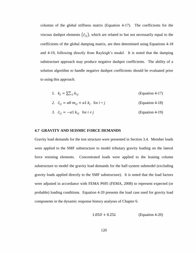
120
columns of the global stiffness matrix (Equation 4-17). The coefficients for the
viscous dashpot elements ( ), which are related to but not necessarily equal to the
coefficients of the global damping matrix, are then determined using Equations 4-18
and 4-19, following directly from Rayleigh’s model. It is noted that the damping
substructure approach may produce negative dashpot coefficients. The ability of a
solution algorithm to handle negative dashpot coefficients should be evaluated prior
to using this approach.
1. ∑
(Equation 4-17)
2. for i = j (Equation 4-18)
3. for i ≠ j (Equation 4-19)
4.7 GRAVITY AND SEISMIC FORCE DEMANDS
Gravity load demands for the test structure were presented in Section 3.4. Member loads
were applied to the SMF substructure to model tributary gravity loading on the lateral
force resisting elements. Concentrated loads were applied to the leaning column
substructure to model the gravity load demands for the half-system submodel (excluding
gravity loads applied directly to the SMF substructure). It is noted that the load factors
were adjusted in accordance with FEMA P695 (FEMA, 2008) to represent expected (or
probable) loading conditions. Equation 4-20 presents the load case used for gravity load
components in the dynamic response history analyses of Chapter 6.
(Equation 4-20)

121
Where
D is the dead load demand
L is the live load demand
The sequential analysis procedure then proceeded as follows:
An initial gravity load analysis was performed using the Static Analysis command.
The loadConst command was used to transfer the model state at the end of the gravity
load analysis to the subsequent earthquake simulation.
Seismic analysis of the test structure was then performed using the Transient Analysis
command. The Transient Integrator for the analysis was set to Newmark Method
(discussed in Section 4.2 and Appendix 1). The Solution Algorithm command was
nested within an iterative subroutine in order to utilize the various solution algorithms
in the OpenSees library, e.g. Modified Newton Algorithm (Appendix 1), Newton
Algorithm, Newton with Line Search Algorithm, and Broyden Algorithm. That is, if
a particular solution algorithm failed to reach convergence within a time step, the
time step was re-analyzed using a different solution algorithm (generally with a more
sophisticated, but computationally expensive routine). The solution algorithms were
nested in order of computational expense in order to improve the efficiency of the
simulation.
Ground acceleration histories were introduced through the Uniform Excitation Load
Pattern command, and were referenced by the interpreter in text file format using the
Time Series command. The effective seismic mass of the test structure was idealized

122
with lumped nodal masses located at the floor levels on the leaning column
substructure. The ground motion ensemble for the earthquake simulations is
discussed in Chapter 5.
4.8 SUMMARY
In order to evaluate the response of the test structure for the maximum considered seismic
hazard (MCE), a nonlinear multi-degree-of-freedom model was developed in the finite
element software OpenSees. The model incorporated three analytical components: (1) a
nonlinear special moment-frame (SMF) substructure used to model lateral load resistance
of a typical N-S SMF; (2) a leaning column substructure used to model tributary mass
and second-order P-delta effects; and (3) a network of equivalent viscous damping
substructures used to model inherent (non-simulated) energy-dissipation mechanisms,
e.g. hysteretic stress-strain response in architectural features and internal friction.
Kinematic constraints were used to tie the dynamic degrees of freedom on the leaning
column substructure to nodes at corresponding floor levels on the SMF and damping
substructures, thereby engaging the lateral resistance of the system during dynamic
response. Gravity load demand for the response history analyses was based on the
expected (or probable) loading condition presented in FEMA P695, and a numerical time
stepping procedure was used to simulate dynamic response of the test structure for an
ensemble of ground acceleration records representative of the maximum considered
seismic hazard (discussed in Chapter 5).

123
Figure 4.1 Nonlinear dynamic response model:
(a) global connectivity; (b) beam-column connection model.
(a)
(b)

Figure 4.2. Fiber element inelastic hinge model.
124

125
Figure 4.3. Uniaxial stress-strain model for A992 steel fibers.
Figure 4.4. Kinematic hardening model (from Mroz, 1967).

126
Figure 4.5. Idealized force system in the beam-column panel zone
(from Charney and Downs, 2004).

(a) (b) (c)
(d) (e) (f)
Figure 4.6 Viscous damping substructures: (a) ; (b) ; (c) ; (d) ; (e) ; (f) .
127

(g) (h)
(i) (j)
Figure 4.6 (continued) Viscous damping substructures: (g) ; (h) ; (i) ; (j) .
128

129
Figure 4.7. Physical interpretation of the global damping
matrix for a shear building (from Charney, 2008).

130
CHAPTER 5
MAXIMUM CONSIDERED
EARTHQUAKE GROUND MOTIONS
5.1 OVERVIEW
This chapter describes the ground motions developed for seismic analysis of the ten-story
steel moment-frame test structure, which was discussed in Chapter 3. Ground shaking
intensity for the site, measured in terms of spectral (or pseudo) acceleration demand, is
discussed in Section 5.2. Sections 5.3 and 5.4 outline the record selection criteria and the
record scaling methodology, respectively. Response characteristics for the scaled ground
motion ensemble are discussed in Section 5.5.
5.2 SPECTRAL ACCELERATION DEMAND
The seismic provisions of ASCE/SEI 7-05 (ASCE, 2005) quantify the maximum
considered earthquake (MCE) hazard for a site in terms of a prescribed pseudo-
acceleration response spectrum, where the pseudo (or spectral) acceleration parameter
was defined in Equation 3-1 of this dissertation. As was discussed in Section 3.5, the
response spectrum is developed from mapped values of short, or 0.2-second, and
1-second period spectral acceleration demand, which are modified by site coefficients to
account for the effect of soil conditions on ground wave propagation (and therefore
ground motion response). The MCE response spectrum based on ASCE/SEI 7-05 is
presented in Figure 5.1. Supporting calculations are provided in Keller and Pessiki
(2011a).

131
In accordance with ASCE/SEI 7-05, the prescribed spectral acceleration demand for the
test structure was determined at the fundamental period of vibration ( ). For the
response history simulations of Chapter 6, the fundamental period of the test structure
was determined from eigenvalue analysis of the multi-degree-of-freedom (MDOF)
dynamic response model developed in Chapter 4, and was found to be 2.3-seconds.
Based on the MCE response spectrum presented in Figure 5.1, the corresponding MCE
spectral acceleration demand was determined to be 0.38 , where denotes gravitational
acceleration.
5.3 GROUND MOTION RECORDS
In order to simulate dynamic response of the test structure for realistic ground shaking, an
ensemble of recorded ground motions from major seismic events was assembled from the
PEER-NGA (Pacific Earthquake Engineering Research Center) database (PEER, 2011)
using the guidelines in FEMA P695 (FEMA, 2008). The Far-Field record set from
FEMA P695, which consists of twenty-two seismic event records, each consisting of two
orthogonal horizontal ground acceleration recordings, was selected to represent the
ground motion hazard for the site. Table 5.1 provides a summary of event and recording
station data for the record ensemble. Site/source data and as-recorded ground motion
response parameters are presented in Tables 5.2 and 5.3, respectively.
The selection criteria developed by FEMA P695 for the Far-Field ground motion
ensemble was based on the following considerations:

132
• Source magnitude (M ≥ 6.5): Large-magnitude events pose the greatest risk of
building collapse due to inherently longer durations of strong shaking and larger
amounts of energy released. Ground motions of smaller magnitude (M < 6.5) events
can cause building damage (typically of a nonstructural nature), but are not likely to
collapse new structures. Even when small magnitude events generate strong ground
motions, the duration of strong shaking is relatively short and the affected area is
relatively small. In contrast, large-magnitude events can generate strong, long
duration, ground motions over a large region, affecting a much larger population of
buildings.
• Source type (strike-slip and thrust source mechanisms): Record sets include
ground motions from earthquakes with either strike-slip or thrust sources. These
sources are typical of shallow crustal earthquakes in California and other Western
United States locations. Few strong-motion records are available from other source
mechanisms.
• Site conditions (soft rock and stiff soil sites): Record sets include ground motions
recorded on either soft rock (Site Class C) or stiff soil (Site Class D) sites. Records
on soft soil (Site Class E) or sites susceptible to ground failure (Site Class F) are not
used. Relatively few strong-motion records are available for Site Class B (rock) sites.
• Site-source distance ( ≥ 10km): The 10 km source-to-site distance boundary
between Near-Field and Far-Field records is arbitrary, but generally consistent with
the “near fault” region of MCE design values mapped in ASCE/SEI 7-05. Several
different measures of this distance are available. For this project, the source-to-site

133
distance was taken as the average of Campbell and Joyner-Boore fault distances
provided in the PEER-NGA database.
• Number of records per event (not more than two): Strong-motion instruments are
not evenly distributed across seismically active regions. Some large-magnitude events
have generated many records, while others have produced only a few, due to the
number of instruments in place at the time of the earthquake. To avoid potential
event-based bias in record sets, not more than two records are taken from any one
earthquake (for a record set). The two-record limit was applied separately to the
Near-Field “Pulse” and “No Pulse” record sets, respectively. When more than two
records of an event pass the other selection criteria, the two records with highest peak
ground velocity are selected.
• Strong ground motion records (PGA > 0.2g and PGV > 15cm/s): The limits on
PGA and PGV are arbitrary, but generally represent the threshold of structural
damage (for new buildings) and capture a large enough sample of the strongest
ground motions (recorded to date) to permit calculation of record-to-record
variability.
• Strong-motion instrument capability (valid frequency content to at least 4-
seconds): Some strong-motion instruments, particularly older models, have inherent
limitations on their ability to record long-period vibration accurately. Most records
have a valid frequency content of at least 8 seconds, but some records do not, and
records not valid to at least 4 seconds are excluded from the record sets. The record
sets are considered valid for collapse evaluation of tall buildings with elastic
fundamental periods up to about 4 seconds.

134
• Strong-motion instrument location (recordings not influenced by structural
response): Strong-motion instruments located in buildings (e.g., ground floor or
basement) can be affected by soil-structure interaction. The records utilized in the
Far-Field set are indicative of the free-field response.
5.4 GROUND MOTION SCALING METHODOLOGY
The scaling methodology of FEMA P695 was used to adjust the ground motion ensemble
developed in Section 5.3 to the MCE demand for the site. The procedure involved the
processes of record normalization and record scaling. A brief description of each process
is provided in the following sections.
5.4.1 Record Normalization
Individual ground motion recordings were normalized with respect to PGV in order to
remove unwarranted variability between records due to inherent differences in event
magnitude, site-source distance, source type, and site conditions, while still maintaining
the inherent aleatory (i.e., record-to-record) variability necessary for characterizing the
seismic hazard. The record normalization procedure is presented in Equations 5-1 and
5-2a-b.
( ) (Equation 5-1)
(Equation 5-2a)
(Equation 5-2b)

135
Where
is the normalization factor applied to both horizontal components of the
ith
record
is the geometric mean of PGV for the ith
record horizontal components
is the median of values for the set
NTH1,i is the normalized ith
record - horizontal component 1
NTH2,i is the normalized ith
record - horizontal component 2
TH1,i is the ith
record - horizontal component 1
TH2,i is the ith
record - horizontal component 2
Table 5.4 provides a summary of normalization factors for the Far-Field record set, and
response parameters for the normalized ground motions. The normalization factors vary
from 0.41 to 2.10 with a median value of 1.00.
5.4.2 Record Scaling
The normalized ground motion ensemble was then collectively scaled at the fundamental
period of the test structure (using a uniform scale factor) so that the median (median of
the geometric mean for each normalized ground motion record pair) spectral acceleration
response equaled the prescriptive spectral acceleration demand from ASCE 7-05.
Conceptually, this approach envisioned the Far-Field record set as representative of a
suite of records from a major earthquake, in which individual records have some
dispersion about an expected value. The scaling procedure is presented in Equations
5-3a-b.

136
(Equation 5-3a)
(Equation 5-3b)
Where
SF is the uniform scale factor for the ground motion ensemble
STH1,i is the normalized and scaled ith
record - horizontal component 1
STH2,i is the normalized and scaled ith
record - horizontal component 2
Table 5.5 presents scaling factors for anchoring the normalized Far-Field record set to the
MCE spectral demand. Response history analyses utilizing the equivalent linear elastic
SDOF dynamic model are presented in Keller and Pessiki (2011a) for each ground
motion record (as-recorded and MCE-scaled). The analyses utilize the explicit Central
Difference numerical time-stepping method.
5.5 CHARACTERISTICS OF THE AS-RECORDED AND MCE-SCALED
GROUND MOTION ENSEMBLES
Time history plots of ground acceleration response for the as-recorded and MCE-scaled
ground motion ensembles are presented in Figures 5.2-5.23, and a summary of response
characteristics is presented in Table 5.6. PGA for the MCE-scaled record set ranged from
0.46g to 1.81g with a median value of 1.16g, and PGV ranged from 76cm/s to 170cm/s
with a median value of 119cm/s. For comparison purposes, the PGA for the as-recorded
record set ranged from 0.15g to 0.82g with a median value of 0.37g, and PGV ranged
from 15cm/s to 115cm/s with a median value of 40cm/s. Spectral acceleration demand
for the MCE-scaled record set (measured at the fundamental period) ranged from 0.38 to

137
2.27 times the value prescribed by ASCE/SEI 7-05. The median spectral acceleration
demand for all records was 1.09 times the ASCE/SEI 7-05 prescribed value.
Figures 5.24-5.45 present the response spectra for the MCE-scaled ground motion
records in the period range of the test structure (response anchored to the fundamental
period of the test structure). A comparison plot of the maximum and median-value
response spectra for the MCE-scaled record ensemble, along with the prescribed MCE
response spectrum from ASCE/SEI 7-05, is presented in Figure 5.46. In general, the
median-value response spectrum for the record ensemble has good correlation with the
ASCE/SEI 7-05 response spectrum for periods at, or larger than, the fundamental period
of the test structure (i.e. the elongated period range), but does produce slightly lower
spectral acceleration demand for periods over approximately 2.5-seconds. For the
maximum-value response spectrum, the spectral acceleration demand over the same
period range is approximately 2-3 times higher than the corresponding ASCE/SEI 7-05
demand. At the fundamental period of the test structure (2.3-seconds), the spectral
acceleration demand for the maximum-value response spectrum is 2.3 times the
ASCE/SEI 7-05 demand.
5.6 SUMMARY
In order to evaluate the dynamic response of the ten-story steel moment-frame test
structure, developed in Chapter 3, for the maximum considered seismic hazard, an
ensemble of ground motion records was assembled from the PEER-NGA database using
the guidelines of FEMA P695. A normalization procedure was utilized to remove

138
unwarranted record variability due to inherent differences in event magnitude, site-source
distance, source type, and site conditions, while still maintaining the inherent aleatory
(i.e., record-to-record) variability necessary for characterizing seismic response. The
ground motion ensemble was then collectively scaled so that the median spectral (or
pseudo) acceleration demand equaled the prescribed MCE-level spectral intensity from
ASCE/SEI 7-05. Conceptually, this approach envisioned the ground motion ensemble as
representative of a suite of records from a major earthquake, in which individual records
have some dispersion about an expected value.
In general, there is good correlation between the median-value response spectrum for the
MCE-scaled record ensemble and the prescribed ASCE/SEI 7-05 MCE response
spectrum over the period range of the test structure. The maximum-value response
spectrum for the MCE-scaled record ensemble is 2-3 times larger than the corresponding
ASCE/SEI 7-05 demand over the same period range.

139
Table 5.1 Summary of earthquake event and recording
station data for the Far-Field record set (from FEMA, 2008)
M Year Name Name Owner
1 6.7 1994 Northridge Beverly Hills - Mulhol USC
2 6.7 1994 Northridge Canyon Country-W LC USC
3 7.1 1999 Duzce, Turkey Bolu ERD
4 7.1 1999 Hector Mine Hector SCSN
5 6.5 1979 Imperial Valley Delta UNAMUCSD
6 6.5 1979 Imperial Valley El Centro Array #11 USGS
7 6.9 1995 Kobe, Japan Nishi-Akashi CUE
8 6.9 1995 Kobe, Japan Shin-Osaka CUE
9 7.5 1999 Kocaeli, Turkey Duzce ERD
10 7.5 1999 Kocaeli, Turkey Arcelik KOERI
11 7.3 1992 Landers Yermo Fire Station CDMG
12 7.3 1992 Landers Coolwater SCE
13 6.9 1989 Loma Prieta Capitola CDMG
14 6.9 1989 Loma Prieta Gilroy Array #3 CDMG
15 7.4 1990 Manjil, Iran Abbar BHRC
16 6.5 1987 Superstition Hills El Centro Imp. Co. CDMG
17 6.5 1987 Superstition Hills Poe Road (temp) USGS
18 7.0 1992 Cape Mendocino Rio Dell Overpass CDMG
19 7.6 1999 Chi-Chi, Taiwan CHY101 CWB
20 7.6 1999 Chi-Chi, Taiwan TCU045 CWB
21 6.6 1971 San Fernando LA - Hollywood Stor CDMG
22 6.5 1976 Friuli, Italy Tolmezzo --
ID No.Earthquake Recording Station

140
Table 5.2 Summary of site and source data
for the Far-Field record set (from FEMA, 2008)
1 D 356 Thrust 13.3 17.2 17.2 9.4
2 D 309 Thrust 26.5 12.4 12.4 11.4
3 D 326 Strike-slip 41.3 12 12.4 12
4 C 685 Strike-slip 26.5 11.7 12 10.4
5 D 275 Strike-slip 33.7 22 22.5 22
6 D 196 Strike-slip 29.4 12.5 13.5 12.5
7 C 609 Strike-slip 8.7 7.1 25.2 7.1
8 D 256 Strike-slip 46 19.2 28.5 19.1
9 D 276 Strike-slip 98.2 15.4 15.4 13.6
10 C 523 Strike-slip 53.7 13.5 13.5 10.6
11 D 354 Strike-slip 86 23.6 23.8 23.6
12 D 271 Strike-slip 82.1 19.7 20 19.7
13 D 289 Strike-slip 9.8 15.2 35.5 8.7
14 D 350 Strike-slip 31.4 12.8 12.8 12.2
15 C 724 Strike-slip 40.4 12.6 13 12.6
16 D 192 Strike-slip 35.8 18.2 18.5 18.2
17 D 208 Strike-slip 11.2 11.2 11.7 11.2
18 D 312 Thrust 22.7 14.3 14.3 7.9
19 D 259 Thrust 32 10 15.5 10
20 C 705 Thrust 77.5 26 26.8 26
21 D 316 Thrust 39.5 22.8 25.9 22.8
22 C 425 Thrust 20.2 15.8 15.8 15
Site Data Site-Source Distance (km)
ID No.
EpicentralClosest to
PlaneCampbell
Joyner-
Boore
Source
(Fault Type)NEHRP
Class
Vs_30
(m/sec)

141
Table 5.3 Summary of PEER-NGA database information and parameters
of recorded ground motions for the Far-Field record set (from FEMA, 2008)
Component 1 Component 2
1 953 0.25 NORTHR/MUL009 NORTHR/MUL279 0.52 63
2 960 0.13 NORTHR/LOS000 NORTHR/LOS270 0.48 45
3 1602 0.06 DUZCE/BOL000 DUZCE/BOL090 0.82 62
4 1787 0.04 HECTOR/HEC000 HECTOR/HEC090 0.34 42
5 169 0.06 IMPVALL/H-DLT262 IMPVALL/H-DLT352 0.35 33
6 174 0.25 IMPVALL/H-E11140 IMPVALL/H-E11230 0.38 42
7 1111 0.13 KOBE/NIS000 KOBE/NIS090 0.51 37
8 1116 0.13 KOBE/SHI000 KOBE/SHI090 0.24 38
9 1158 0.24 KOCAELI/DZC180 KOCAELI/DZC270 0.36 59
10 1148 0.09 KOCAELI/ARC000 KOCAELI/ARC090 0.22 40
11 900 0.07 LANDERS/YER270 LANDERS/YER360 0.24 52
12 848 0.13 LANDERS/CLW -LN LANDERS/CLW -TR 0.42 42
13 752 0.13 LOMAP/CAP000 LOMAP/CAP090 0.53 35
14 767 0.13 LOMAP/G03000 LOMAP/G03090 0.56 45
15 1633 0.13 MANJIL/ABBAR--L MANJIL/ABBAR--T 0.51 54
16 721 0.13 SUPERST/B-ICC000 SUPERST/B-ICC090 0.36 46
17 725 0.25 SUPERST/B-POE270 SUPERST/B-POE360 0.45 36
18 829 0.07 CAPEMEND/RIO270 CAPEMEND/RIO360 0.55 44
19 1244 0.05 CHICHI/CHY101-E CHICHI/CHY101-N 0.44 115
20 1485 0.05 CHICHI/TCU045-E CHICHI/TCU045-N 0.51 39
21 68 0.25 SFERN/PEL090 SFERN/PEL180 0.21 19
22 125 0.13 FRIULI/A-TMZ000 FRIULI/A-TMZ270 0.35 31
PEER-NGA Record Information Recorded Motions
File Names - Horizontal RecordsID No.
Record
Seq. No.
Lowest
Freq (Hz.)
PGAmax
(g)
PGVmax
(cm/s.)

142
Table 5.4 Summary of factors used to normalize recorded ground motions,
and parameters of normalized ground motions for the Far-Field record set
(from FEMA, 2008)
Comp. 1 Comp. 2
1 1.02 0.94 57.2 0.65 0.34 41
2 0.38 0.63 44.8 0.83 0.40 38
3 0.72 1.16 59.2 0.63 0.52 39
4 0.35 0.37 34.1 1.09 0.37 46
5 0.26 0.48 28.4 1.31 0.46 43
6 0.24 0.23 36.7 1.01 0.39 43
7 0.31 0.29 36.0 1.03 0.53 39
8 0.33 0.23 33.9 1.10 0.26 42
9 0.43 0.61 54.1 0.69 0.25 41
10 0.11 0.11 27.4 1.36 0.30 54
11 0.50 0.33 37.7 0.99 0.24 51
12 0.20 0.36 32.4 1.15 0.48 49
13 0.46 0.28 34.2 1.09 0.58 38
14 0.27 0.38 42.3 0.88 0.49 39
15 0.35 0.54 47.3 0.79 0.40 43
16 0.31 0.25 42.8 0.87 0.31 40
17 0.33 0.34 31.7 1.17 0.53 42
18 0.54 0.39 45.4 0.82 0.45 36
19 0.49 0.95 90.7 0.41 0.18 47
20 0.30 0.43 38.8 0.96 0.49 38
21 0.25 0.15 17.8 2.10 0.44 40
22 0.25 0.30 25.9 1.44 0.50 44
As-Recorded Parameters Normalized Motions
1-Sec. Spec. Acc. (g)ID No.PGAmax
(g)
PGVmax
(cm/s)
Normalization
FactorPGVPEER
(cm/s)

143
Table 5.5 Scaling factors for anchoring the Far-Field record
set to the MCE spectral demand (from FEMA, 2008)
Dmin Cmin Bmin
0.25 0.936 0.779 1.93 0.96 0.64 0.32
0.30 1.020 0.775 1.94 0.97 0.65 0.32
0.35 0.939 0.761 1.97 0.99 0.66 0.33
0.40 0.901 0.748 2.00 1.00 0.67 0.33
0.45 0.886 0.749 2.00 0.89 0.59 0.30
0.50 0.855 0.736 2.04 0.82 0.54 0.27
0.60 0.833 0.602 2.49 0.83 0.55 0.28
0.70 0.805 0.537 2.40 0.80 0.53 0.27
0.80 0.739 0.449 2.50 0.83 0.56 0.28
0.90 0.633 0.399 2.50 0.83 0.56 0.28
1.00 0.571 0.348 2.59 0.86 0.58 0.29
1.20 0.476 0.301 2.49 0.83 0.55 0.28
1.40 0.404 0.256 2.51 0.84 0.56 0.28
1.60 0.356 0.208 2.70 0.90 0.60 0.30
1.80 0.319 0.168 2.98 0.99 0.66 0.33
2.00 0.284 0.148 3.05 1.02 0.68 0.34
2.20 0.258 0.133 3.08 1.03 0.68 0.34
2.40 0.230 0.118 3.18 1.06 0.71 0.35
2.60 0.210 0.106 3.28 1.09 0.73 0.36
2.80 0.190 0.091 3.53 1.18 0.79 0.39
3.00 0.172 0.080 3.75 1.25 0.83 0.42
3.50 0.132 0.063 4.10 1.37 0.91 0.46
4.00 0.104 0.052 4.29 1.43 0.95 0.48
4.50 0.086 0.046 4.34 1.45 0.96 0.48
5.00 0.072 0.041 4.43 1.48 0.98 0.49
Period
T = Cu Ta
(seconds)
Median Value of
Normalized Record Set,
SNRT (g)
Scaling Factors for Anchoring
Far-Field Record Set to MCE
Spectral Demand
Dmax Cmax BmaxNear-Field
Set
Far-Field
Set

Table 5.6 Characteristics of the as-recorded and MCE-scaled ground motion ensembles
PGA (g) PGV (cm/s) NM SF Total PGA (g) PGV (cm/s) SMT/SMT
1A NORTHR/MUL009 0.16 0.42 59 0.65 3.15 2.05 0.85 121 0.99
1B NORTHR/MUL279 0.25 0.52 63 0.65 3.15 2.05 1.06 129 0.82
2A NORTHR/LOS000 0.05 0.41 43 0.83 3.15 2.61 1.07 112 1.56
2B NORTHR/LOS270 0.13 0.48 45 0.83 3.15 2.61 1.26 118 0.79
3A DUZCE/BOL000 0.05 0.73 56 0.63 3.15 1.98 1.44 112 1.10
3B DUZCE/BOL090 0.05 0.82 62 0.63 3.15 1.98 1.63 123 0.78
4A HECTOR/HEC000 0.03 0.27 29 1.09 3.15 3.43 0.91 98 0.82
4B HECTOR/HEC090 0.04 0.34 42 1.09 3.15 3.43 1.16 143 1.29
5A IMPVALL/H-DLT262 0.06 0.24 26 1.31 3.15 4.13 0.98 107 1.45
5B IMPVALL/H-DLT352 0.06 0.35 33 1.31 3.15 4.13 1.45 136 1.68
6A IMPVALL/H-E11140 0.25 0.36 35 1.01 3.15 3.18 1.16 110 1.36
6B IMPVALL/H-E11230 0.13 0.38 42 1.01 3.15 3.18 1.21 134 0.90
7A KOBE/NIS000 0.13 0.51 37 1.03 3.15 3.24 1.65 121 1.75
7B KOBE/NIS090 0.13 0.50 37 1.03 3.15 3.24 1.63 119 1.33
8A KOBE/SHI000 0.13 0.24 38 1.10 3.15 3.47 0.84 131 1.30
8B KOBE/SHI090 0.10 0.21 28 1.10 3.15 3.47 0.73 97 0.85
9A KOCAELI/DZC180 0.24 0.31 59 0.69 3.15 2.17 0.68 128 1.53
9B KOCAELI/DZC270 0.10 0.36 46 0.69 3.15 2.17 0.78 101 1.43
10A KOCAELI/ARC000 0.09 0.22 18 1.36 3.15 4.28 0.94 76 0.38
10B KOCAELI/ARC090 0.05 0.15 40 1.36 3.15 4.28 0.64 170 0.78
11A LANDERS/YER270 0.07 0.25 52 0.99 3.15 3.12 0.76 160 1.13
11B LANDERS/YER360 0.07 0.15 30 0.99 3.15 3.12 0.47 93 0.61
Record ID PEER-NGA File NameLowest Usable
Frequency (Hz)
Unscaled Record Scaled RecordScale Factors
144

Table 5.6 (continued) Characteristics of the as-recorded and MCE-scaled ground motion ensembles
PGA (g) PGV (cm/s) NM SF Total PGA (g) PGV (cm/s) SMT/SMT
12A LANDERS/CLW-LN 0.13 0.28 26 1.15 3.15 3.62 1.03 93 0.43
12B LANDERS/CLW-TR 0.13 0.42 42 1.15 3.15 3.62 1.51 154 0.84
13A LOMAP/CAP000 0.25 0.53 35 1.09 3.15 3.43 1.81 120 1.00
13B LOMAP/CAP090 0.25 0.44 29 1.09 3.15 3.43 1.52 100 0.52
14A LOMAP/G03000 0.13 0.56 36 0.88 3.15 2.77 1.54 99 0.39
14B LOMAP/G03090 0.13 0.37 45 0.88 3.15 2.77 1.02 124 1.70
15A MANJIL/ABBAR-L 0.13 0.52 43 0.79 3.15 2.49 1.28 106 1.45
15B MANJIL/ABBAR-T 0.13 0.50 52 0.79 3.15 2.49 1.24 129 2.27
16A SUPERST/B-ICC000 0.13 0.36 46 0.87 3.15 2.74 0.98 127 1.14
16B SUPERST/B-ICC090 0.13 0.26 41 0.87 3.15 2.74 0.71 112 1.88
17A SUPERST/B-POE270 0.25 0.45 36 1.17 3.15 3.69 1.65 132 1.55
17B SUPERST/B-POE360 0.09 0.30 33 1.17 3.15 3.69 1.11 121 1.64
18A CAPEMEND/RIO270 0.07 0.39 44 0.82 3.15 2.58 1.00 113 0.76
18B CAPEMEND/RIO360 0.07 0.55 42 0.82 3.15 2.58 1.42 108 0.40
19A CHICHI/CHY101-E 0.04 0.35 71 0.41 3.15 1.29 0.46 91 1.08
19B CHICHI/CHY101-N 0.05 0.44 115 0.41 3.15 1.29 0.57 149 1.59
20A CHICHI/TCU045-E 0.03 0.47 37 0.96 3.15 3.02 1.43 111 0.69
20B CHICHI/TCU045-N 0.05 0.51 39 0.96 3.15 3.02 1.55 118 0.76
21A SFERN/PEL090 0.25 0.21 19 2.10 3.15 6.62 1.39 125 1.34
21B SFERN/PEL180 0.25 0.17 15 2.10 3.15 6.62 1.15 98 1.56
22A FRIULI/A-TMZ000 0.13 0.35 22 1.44 3.15 4.54 1.59 100 0.57
22B FRIULI/A-TMZ270 0.13 0.32 31 1.44 3.15 4.54 1.43 140 0.51
Record ID PEER-NGA File NameLowest Usable
Frequency (Hz)
Unscaled Record Scale Factors Scaled Record
145

146
Figure 5.1 ASCE/SEI 7-05 MCE response spectrum.

Figure 5.2 Northridge, CA, 1994: (a) EQ1A NORTHR/MUL009; (b) EQ1B NORTHR/MUL279.
Figure 5.3 Northridge, CA, 1994: (a) EQ2A NORTHR/LOS000; (b) EQ2B NORTHR/LOS270.
147
(a) (b)
(a) (b)
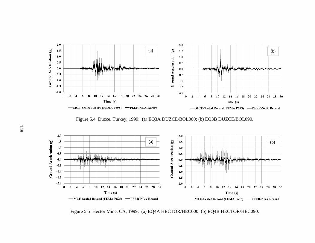
Figure 5.4 Duzce, Turkey, 1999: (a) EQ3A DUZCE/BOL000; (b) EQ3B DUZCE/BOL090.
Figure 5.5 Hector Mine, CA, 1999: (a) EQ4A HECTOR/HEC000; (b) EQ4B HECTOR/HEC090.
148
(a) (b)
(a) (b)

Figure 5.6 Imperial Valley, CA, 1979: (a) EQ5A IMPVALL/H-DLT262; (b) EQ5B IMPVALL/H-DLT352.
Figure 5.7 Imperial Valley, CA, 1979: (a) EQ6A IMPVALL/H-E11140; (b) EQ6B IMPVALL/H-E11230.
149
(a) (b)
(a) (b)

Figure 5.8 Kobe, Japan, 1995: (a) EQ7A KOBE/NIS000; (b) EQ7B KOBE/NIS090.
Figure 5.9 Kobe, Japan, 1995: (a) EQ8A KOBE/SHI000; (b) EQ8B KOBE/SHI090.
150
(a)
(a)
(b)
(b)

Figure 5.10 Kocaeli, Turkey, 1999: (a) EQ9A KOCAELI/DZC180; (b) EQ9B KOCAELI/DZC270.
Figure 5.11 Kocaeli, Turkey, 1999: (a) EQ10A KOCAELI/ARC000; (b) EQ10B KOCAELI/ARC090.
151
(a)
(a)
(b)
(b)

Figure 5.12 Landers, CA, 1992: (a) EQ11A LANDERS/YER270; (b) EQ11B LANDERS/YER360.
Figure 5.13 Landers, CA, 1992: (a) EQ12A LANDERS/CLW-LN; (b) EQ12B LANDERS/CLW-TR.
152
(a)
(a)
(b)
(b)

Figure 5.14 Loma Prieta, CA, 1989: (a) EQ13A LOMAP/CAP000; (b) EQ13B LOMAP/CAP090.
Figure 5.15 Loma Prieta, CA, 1989: (a) EQ14A LOMAP/G03000; (b) EQ14B LOMAP/G03090.
153
(a)
(a)
(b)
(b)

Figure 5.16 Manjil, Iran, 1990: (a) EQ15A MANJIL/ABBAR-L; (b) EQ15B MANJIL/ABBAR-T.
Figure 5.17 Superstition Hills, CA, 1987: (a) EQ16A SUPERST/B-ICC000; (b) EQ16B SUPERST/B-ICC090.
154
(a)
(a)
(b)
(b)

Figure 5.18 Superstition Hills, CA, 1987: (a) EQ17A SUPERST/B-POE270; (b) EQ17B SUPERST/B-POE360.
Figure 5.19 Cape Mendocino, CA, 1992: (a) EQ18A CAPEMEND/RIO270; (b) EQ18B CAPEMEND/RIO360.
155
(a)
(a)
(b)
(b)

Figure 5.20 Chi-Chi, Taiwan, 1999: (a) EQ19A CHICHI/CHY101-E; (b) EQ19B CHICHI/CHY101-N.
Figure 5.21 Chi-Chi, Taiwan, 1999: (a) EQ20A CHICHI/TCU045-E; (b) EQ20B CHICHI/TCU045-N.
156
(a) (b)
(a) (b)

Figure 5.22 San Fernando, CA, 1971: (a) EQ21A SFERN/PEL090; (b) EQ21B SFERN/PEL180.
Figure 5.23 Friuli, Italy, 1976: (a) EQ22A FRIULI/A-TMZ000; (b) EQ22B FRIULI/A-TMZ270.
157
(a)
(a)
(b)
(b)

Figure 5.24 MCE-scaled response spectrum, ζ=5%: (a) EQ1A NORTHR/MUL009; (b) EQ1B NORTHR/MUL279.
Figure 5.25 MCE-scaled response spectrum, ζ=5%: (a) EQ2A NORTHR/LOS000; (b) EQ2B NORTHR/LOS270.
158
(a) (b)
(a) (b)

Figure 5.26 MCE-scaled response spectrum, ζ=5%: (a) EQ3A DUZCE/BOL000; (b) EQ3B DUZCE/BOL090.
Figure 5.27 MCE-scaled response spectrum, ζ=5%: (a) EQ4A HECTOR/HEC000; (b) EQ4B HECTOR/HEC090.
159
(a)
(a)
(b)
(b)

Figure 5.28 MCE-scaled response spectrum, ζ=5%: (a) EQ5A IMPVALL/H-DLT262; (b) EQ5B IMPVALL/H-DLT352.
Figure 5.29 MCE-scaled response spectrum, ζ=5%: (a) EQ6A IMPVALL/H-E11140; (b) EQ6B IMPVALL/H-E11230.
160
(a)
(b)
(a) (b)
Figure 5.30 MCE-scaled response spectrum, ζ=5%: (a) EQ7A KOBE/NIS000; (b) EQ7B KOBE/NIS090.
Figure 5.31 MCE-scaled response spectrum, ζ=5%: (a) EQ8A KOBE/SHI000; (b) EQ8B KOBE/SHI090.
161
(a) (b)
(a) (b)

Figure 5.32 MCE-scaled response spectrum, ζ=5%: (a) EQ9A KOCAELI/DZC180; (b) EQ9B KOCAELI/DZC270.
Figure 5.33 MCE-scaled response spectrum, ζ=5%: (a) EQ10A KOCAELI/ARC000; (b) EQ10B KOCAELI/ARC090.
162
(a)
(a)
(b)
(b)

Figure 5.34 MCE-scaled response spectrum, ζ=5%: (a) EQ11A LANDERS/YER270; (b) EQ11B LANDERS/YER360.
Figure 5.35 MCE-scaled response spectrum, ζ=5%: (a) EQ12A LANDERS/CLW-LN; (b) EQ12B LANDERS/CLW-TR.
163
(a)
(a)
(b)
(b)

Figure 5.36 MCE-scaled response spectrum, ζ=5%: (a) EQ13A LOMAP/CAP000; (b) EQ13B LOMAP/CAP090.
Figure 5.37 MCE-scaled response spectrum, ζ=5%: (a) EQ14A LOMAP/G03000; (b) EQ14B LOMAP/G03090.
164
(a) (b)
(a) (b)

Figure 5.38 MCE-scaled response spectrum, ζ=5%: (a) EQ15A MANJIL/ABBAR-L; (b) EQ15B MANJIL/ABBAR-T.
Figure 5.39 MCE-scaled response spectrum, ζ=5%: (a) EQ16A SUPERST/B-ICC000; (b) EQ16B SUPERST/B-ICC090.
165
(a)
(a)
(b)
(b)

Figure 5.40 MCE-scaled response spectrum, ζ=5%: (a) EQ17A SUPERST/B-POE270; (b) EQ17B SUPERST/B-POE360.
Figure 5.41 MCE-scaled response spectrum, ζ=5%: (a) EQ18A CAPEMEND/RIO270; (b) EQ18B CAPEMEND/RIO360.
166
(a)
(a)
(b)
(b)

Figure 5.42 MCE-scaled response spectrum, ζ=5%: (a) EQ19A CHICHI/CHY101-E; (b) EQ19B CHICHI/CHY101-N.
Figure 5.43 MCE-scaled response spectrum, ζ=5%: (a) EQ20A CHICHI/TCU045-E; (b) EQ20B CHICHI/TCU045-N.
167
(a)
(a) (b)
(b)

Figure 5.44 MCE-scaled response spectrum, ζ=5%: (a) EQ21A SFERN/PEL090; (b) EQ21B SFERN/PEL180.
Figure 5.45 MCE-scaled response spectrum, ζ=5%: (a) EQ22A FRIULI/A-TMZ000; (b) EQ22B FRIULI/A-TMZ270.
168
(a)
(a) (b)
(b)

169
Figure 5.46 Response spectrum for the MCE-scaled record ensemble, ζ=5%.

170
CHAPTER 6
RESPONSE OF THE TEST STRUCTURE
FOR THE MAXIMUM CONSIDERED SEISMIC HAZARD
6.1 OVERVIEW
This chapter presents results from nonlinear response history analyses utilizing the multi-
degree-of-freedom (MDOF) dynamic response model developed in Chapter 4 and the
maximum considered earthquake (MCE) ground motion ensemble developed in
Chapter 5. The numerical simulations were performed in the finite element software
OpenSees (OpenSees, 2011). The objective of this task was to characterize force and
deformation demands in the test structure for the MCE hazard, and to develop damaged
structural models for the post-earthquake fire simulations of Chapters 7-10.
The monotonic lateral load response of the test structure, as determined from a nonlinear
displacement-controlled (pushover) analysis, is discussed in Section 6.2. Drift demand
and residual force recordings from nonlinear response history analyses are presented in
Sections 6.3 and 6.4, respectively. Section 6.5 presents a comparison of lateral strength
and drift estimates from the nonlinear MDOF simulations with the prescriptive response
modification factors utilized in the equivalent lateral force (ELF) design procedure of
ASCE/SEI 7-05 (ASCE/SEI, 2005). Deformation demands in a representative moment-
frame beam-column connection are discussed in Section 6.6. Finally, the frequency of
exceedance for several large magnitude drift demands, representative of potential
thresholds for SFRM damage, are presented in Section 6.7.

171
6.2 MONOTONIC LATERAL LOAD RESPONSE
6.2.1 Lateral Strength and Ductility
Figure 6.1 presents the base shear resistance of the test structure in the N-S direction as a
function of roof drift demand, as determined from a nonlinear monotonic displacement-
controlled pushover analysis. The load pattern for the pushover analysis was based on
the idealized inertial force distribution calculated in Equation 3-11. The base shear
capacity ( ) is approximately 17% of the seismic weight. The roof displacement at
the effective linear limit ( ) and roof displacement capacity ( ) were determined
using the guidelines in FEMA P695 (FEMA, 2008). The roof displacement at the
effective linear limit, which was taken as the displacement where a line through the
origin and a point at 60% of the base shear ( ) reaches (as shown in Figure
6.2), was determined to be 0.88%. The roof displacement capacity was taken as the point
of 20% strength loss ( ) and was determined to be 5.5%
The corresponding structural system collapse ductility ( ), defined as the ratio of roof
drift capacity to roof drift at the effective linear limit, was then determined using
Equation 6-1.
⁄ ⁄
(Equation 6-1)
The system overstrength factor ( ), defined as the ratio of the maximum base shear
resistance to the design base shear, was determined using Equation 6-2.

172
⁄
⁄
(Equation 6-2)
6.2.2 Secant Stiffness
The monotonic pushover analysis was also used to quantify post-yield secant stiffness of
the test structure, defined as the slope of the secant line between the origin and the point
on the pushover curve at the roof drift of interest. Since ground shaking records have a
usable frequency range related to instrument sensitivity and/or record filtering, period
elongation of the structural system during nonlinear softening could potentially shift
vibratory motion of the building into an artificial “zero energy” region if the elongated
period exceeds the useable frequency content of the record. In this scenario, the structure
is no longer excited by forced vibration at the secant period. This limitation with certain
ground motion records may result in an underestimation of inertial force and drift
demands in the elongated period range. As a result, the secant period of the structure at
peak drift demand for each record was checked against the useable frequency content for
the record. Suitability of the MCE record ensemble is discussed in the Section 6.4.
6.3 DRIFT DEMANDS
Time history recordings of roof drift are provided for each earthquake simulation in
Figures 6.3-6.24. Peak and residual interstory drift demands, which are presented in
terms of an interstory drift ratio (IDR) equal to the drift demand in the story normalized
by respective story height, are presented in Figures 6.25-6.46. The concurrent lateral
floor displacements recorded at peak roof drift demand and at the end of the simulation

173
(residual post-earthquake state) are plotted in Figures 6.47-6.68. The results are
summarized in Tables 6.1 and 6.2.
Only one of the forty-four ground motion records (EQ5B) induced sidesway collapse of
the test structure. For the purposes of this study, sidesway collapse was assumed to occur
at the following response limits: (1) an IDR demand of 6.4%, which is consistent with the
probable rotational capacity of welded unreinforced flange – welded web (WUF-W)
moment-frame beam-column connections published in FEMA 350 (FEMA, 2000); or (2)
a peak roof drift demand of 5.5%, which is based on the roof displacement capacity
calculated in Section 6.2.1.
Excluding record EQ5B from the data set, the maximum recorded IDR demand in the test
structure ranged from 1.3% to 4.9%, with a median value of 2.8%. The maximum
residual IDR demand ranged from 0.1% to 3.9%, with a median value of 1%. Peak roof
drift demand ranged from 0.7% to 3.4%, with a median value of 1.5%.
Figure 6.69 shows a correlation between peak IDR demand predicted by nonlinear
MDOF response history analyses and pseudo-acceleration demand predicted by
equivalent linear elastic SDOF analyses based on the fundamental mode of vibration. It
is noted, however, that dispersion of the response data is significantly greater at larger
drift demands. This can be attributed to a large variation in low frequency (long period)
content among the ground motion records. As critically stressed elements in the structure
yield during seismic response, the lateral resistance of the building system softens and the

174
structure effectively vibrates at an elongated period. This period elongation generally
lowers the transmissibility between the ground shaking and the vibrating structure since
the natural frequencies of the damaged building shift into a range of low energy content
(for typical ground motions). Low frequency content of the ground motion record
(whether natural or influenced by artificial filtering as discussed in Section 6.2.2)
therefore becomes a critical parameter in driving inertial forces and deformation demands
in the softened structure. This characteristic is particularly evident for the ten-story test
structure, which has a relatively long fundamental period with respect to typical ground
motion frequency content.
Dispersion of the response data is more pronounced for the case of residual IDR demand,
as shown in Figure 6.69. Residual deformations are generally influenced by peak
inelastic excursions and are therefore dependent on the aforementioned variability in low
frequency ground motion content. In addition, residual deformations are also influenced
by directionality of the dynamic response. Ground motion records that induce a near-
symmetric dynamic response in the structure are more likely to produce smaller residual
drift demands than ground motion records that favor peak displacement response in a
particular direction (i.e. similar to the response to a pulse excitation).
6.4 SUITABILITY OF THE MCE GROUND MOTION RECORD ENSEMBLE
Table 6.3 presents a comparison of usable frequency content (and the corresponding
equivalent cut-off periods) for the MCE-scaled ground motion records with the secant
periods calculated at peak roof drift demand. The critical secant period-to-cut-off period

175
ratio ranged from 0.07 to 1.03 with a median value of 0.31. It is noted that only one
record (EQ21A) produced a ratio larger than 1.0, indicating the potential loss of
transmissibility in an artificial “zero energy” response range (discussed in Section 6.2).
Due to the limited number of records in the data set, the EQ21A response record was
retained for statistical purposes.
6.5 COMPARISON OF INHERENT DAMPING MODELS
Figure 6.70 presents a comparison of displacement history at the roof level for two
MDOF dynamic response models for the test structure: (a) an MDOF dynamic response
model employing the damping substructure approach developed in Chapter 4; (b) and an
MDOF dynamic response model utilizing conventional Rayleigh mass and stiffness-
proportional damping specified at the element level. The numerical problems associated
with using conventional Rayleigh damping for nonlinear dynamic analyses were
discussed in Chapter 4. As expected, the peak roof drift demand for the damping
substructure approach (2.49%) is slightly larger than the value attained using
conventional Rayleigh damping (2.31%), which leads to an increase in residual drift
demand of 0.21%. As discussed in Chapter 4, the discrepancy in drift demand between
the two models is due to the development of artificially high viscous forces in the model
with conventional Rayleigh damping.
6.6 RESIDUAL DESTABILIZING FORCES
Residual destabilizing moments at the 4th
elevated floor are presented in Table 6.2, and
are plotted with respect to pseudo-acceleration demand in Figure 6.71. The values range

176
from 0.01% to 4.4% of the base moment capacity of the structure, with a median value of
0.6%. Similar to the residual IDR demands, there is significant scatter in the response
data. This can be attributed to the same variability discussed in the preceding section for
residual drift demands. In addition, the influence of higher mode effects can alter the
relative shape of the deformed configuration and therefore affect second-order
destabilizing moment acting at a particular story.
6.7 EVALUATION OF RESPONSE MODIFICATION FACTORS FOR THE
ASCE/SEI 7-05 ELF DESIGN PROCEDURE
Table 6.4 presents a comparison of strength and drift response parameters developed
from nonlinear pushover and response history analyses along with corresponding values
utilized in the ELF design procedure. The ELF response modification factors were
defined schematically in Figures 3.5 and 3.6.
The system overstrength factor ( ) was defined in Equation 3-8 as the ratio of the
maximum base shear resistance ( ) to the design base shear ( ), and was
determined from Equation 6-2 to be 4.25. This value is 42% larger than the overstrength
factor of 3.0 prescribed by ASCE/SEI 7-05 for buildings utilizing steel special moment-
frames. The prescriptive overstrength factor in ASCE/SEI 7-05 therefore appears to
provide a conservative estimate of lateral load capacity, although it is acknowledged that
overstrength could vary significantly with frame geometry.

177
The strength modification factor ( ) was defined in Equation 3-7 as the ratio of the force
level that would be developed in the system for design earthquake ground motions, if the
system remained entirely linearly elastic ( ), to the base shear prescribed for design
( ). A parallel to the roof drift-base shear relationship of Figure 3.5 was presented
in Figure 3.6 in terms of spectral coordinates. In Figure 3.6, the term SMT is the MCE
spectral (or pseudo) acceleration demand at the fundamental period of the system. An
alternative definition of the strength modification factor ( ) can therefore be taken as:
( ) (Equation 6-3)
Where
is the ratio between the MCE spectral acceleration demand ( ) and the
design-basis earthquake (DBE) spectral acceleration demand ( ), taken as
1.5.
is the DBE seismic coefficient, defined in Equation 3-10.
Based on this definition, an equivalent strength modification factor was determined for
each of the MCE-scaled response history simulations. As shown in Table 6.4, the
calculated strength modification factors ranged from 2.5 to 15 with a median value of 7.3.
This median value of 7.3 is slightly lower than the value of 8 prescribed by ASCE 7-05.
A lower -value leads to larger lateral load demands and a more conservative design.
The deflection amplification factor ( ) was defined in Equation 3-9 and is utilized in the
design process to estimate peak lateral deflection demand for the DBE by amplifying

178
results from a linear elastic analysis. Equivalent estimates of displacement demand for
the MCE can be developed using Equation 6-4.
( )
( )⁄ (Equation 6-4)
Where
is the deflection amplification factor for MCE-scaled ground motions
is the deflection demand for MCE-scaled ground motions considering
linear elastic response
is deflection demand for DBE-scaled ground motions considering
nonlinear inelastic response
As shown in Table 6.4, the calculated MCE deflection amplification factors ranged from
3.7 to 19 with a median value of 8.3. This median value is identical to the MCE-scaled
deflection amplification factor prescribed by ASCE/SEI 7-05.
6.8 DEFORMATION DEMANDS IN MOMENT-FRAME BEAM-COLUMN
CONNECTION CONNC2F4
In order to evaluate deformation demands in moment-frame beam-column connections
for the MCE hazard, a representative interior connection along the 4th
elevated floor
(designated as ConnC2F4) was selected as an analytical test specimen. This location,
which was presented in Figure 4.1, was chosen based on the following considerations:
(1) peak IDR recordings in the lower story larger than 3% (indicative of rotational
demand in the beam-column connections along the floor line and probable damage to

179
spray-applied fire-resistive insulation based on test results from Braxtan and Pessiki
(2009, 2011a, 2011b); and (2) large residual IDR recordings in the upper floors
(indicative of residual destabilizing moment).
The deformation response in ConnC2F4 was then evaluated for two MCE records:
EQ11A (Landers, CA, 1992) and EQ17A (Superstition Hills, CA, 1987). Records
EQ11A and EQ17A were selected based on the following considerations: (1) both
records produced peak rotational demands in ConnC2F4 (measured in terms of the drift
angle parameter defined in FEMA 350 (FEMA, 2000)) larger than 3%, indicating a high
probability for damage to spray-applied fire-resistive insulation; (2) both records
produced large destabilizing moment at the 4th
elevated floor relative to the MCE record
ensemble (related to the fire compartment locations for the post-earthquake fire
simulations of Chapters 9 and 10); (3) both records were from southern California events
and were therefore consistent with the site conditions assumed in the design process; and
(4) both records were from relatively recent events and were obtained using modern
recording devices.
It is noted that while the fiber element beam-column hinges (discussed in Section 4.4.2)
are able to model inelastic stress-strain response in the connection due to material
yielding (material nonlinearity), they are unable to account for softening due to local
buckling distortions in the compression flanges (geometric softening). The implications
of this idealization are addressed in Chapter 7.

180
6.8.1 EQ11A LANDERS/YER270
Figure 6.72 presents a time history plot of rotational demand in ConnC2F4 for the
EQ11A ground motion record. Rotational demand is measured in terms of the drift angle
parameter defined in FEMA 350. Corresponding strain demands in the beam and column
hinge regions are presented in Figures 6.73 and 6.74, respectively. Time history
recordings for panel zone shear deformation and column flange flexure are presented in
Figure 6.75.
During the first few seconds of the ground motion simulation, the rotational demand in
the connection oscillates about the deformed position at the end of the gravity load step.
First yield in the beam flanges occurs at 13-seconds into the simulation at a drift angle of
0.8%. The concurrent strain demands in the column flanges and panel zone are 64% and
53%, respectively, of the nominal yield strain. Strain demands in the column flanges
within the panel zone are small.
At approximately 16-seconds into the simulation, inertial forces in the building drive
rotational demand in the connection to a peak positive drift angle of 1.8%. Inelastic
deformations are concentrated in the beam flanges where strain demands reach 17 times
the nominal yield strain. The concurrent strain demands in the column flanges and panel
zone reach 67% and 65%, respectively, of the nominal yield strain. Strain demands in the
column flanges within the panel zone remain small.

181
Immediately following this positive peak, a combination of elastic restoring forces and
ground acceleration-induced inertial force demands cause the building to surge in the
opposite direction. The connection rotates to peak drift angle of -2.8%. Strain demands
in the beam flanges reach 34 times the nominal yield strain. Concurrent strain demands
in the column flanges and panel zone reach 70% and 65%, respectively, of nominal yield
strain. Strain demands in the column flanges within the panel zone remain small.
Beyond this negative peak, rotational demand in the connection effectively oscillates
about a residual drift angle of approximately -2%.
The peak rotational demand of -3.5% occurs at 32-seconds into the simulation. Strain
demands in the beam flanges reach 46 times the nominal yield strain. Concurrent strain
demands in the column flanges and panel zone reach 71% and 67%, respectively, of
nominal yield strain. Strain demands in the column flanges within the panel zone remain
small.
By 60-seconds into the simulation, damping mechanisms in the test structure have
essentially brought the system to rest. Residual inelastic deformations in the moment-
frame substructure lock the connection into a residual drift angle of 1.9%.
6.8.2 EQ17A SUPERST/B-POE270
Figure 6.76 presents a time history plot of rotational demand in ConnC2F4 for the
EQ17A ground motion record. Corresponding strain demands in the beam and column
hinge regions are presented in Figures 6.77 and 6.78, respectively. Time history

182
estimates for panel zone shear deformation and column flange bending are presented in
Figure 6.79.
Similar to the EQ11A response record, the rotational demand in the connection initially
oscillates about the deformed position at the end of the gravity load step. First yield in
the beam flanges occurs at 4-seconds into the simulation at a drift angle of 0.8%. The
concurrent strain demands in the column flanges and panel zone are 60% and 53%,
respectively, of the nominal yield strain. Strain demands in the column flanges within the
panel zone are small.
At approximately 7-seconds into the simulation, inertial forces in the building drive
rotational demand in the connection to a drift angle of 3.6%. Inelastic deformations are
concentrated in the beam flanges where strain demands reach 43 times the nominal yield
strain. Critical strain demands in the lower column hinge region exceed the nominal
yield strain by 6%, and the concurrent shear strain demand in the panel zone reaches 67%
of the nominal yield strain. Strain demands in the column flanges within the panel zone
remain small.
Immediately following this positive peak, a combination of elastic restoring forces and
ground acceleration-induced inertial force demands cause the building to surge in the
opposite direction, and the connection rotates to a drift angle of 0.1%. Plastic strains in
the beam flanges recede to 18 times the nominal yield strain. Concurrent strain demands

183
in the column flanges and panel zone drop to 81% and 64%, respectively, of the nominal
yield strain. Strain demands in the column flanges within the panel zone remain small.
Inertial and restoring forces in the structure then drive the rotational demand in the
connection to a peak value of 3.5%, which occurs at approximately 9.5-seconds into the
simulation. Strain demands in the beam flanges reach 46 times the nominal yield strain.
Concurrent strain demands in the column flanges and panel zone reach 97% and 60%,
respectively, of nominal yield strain. Strain demands in the column flanges within the
panel zone remain small. After this point the rotational demand in the connection
effectively oscillate about a residual drift of 2.2%.
By 60-seconds into the simulation, damping mechanisms in the test structure have
essentially brought the system to rest. Residual inelastic deformations in the moment-
frame substructure lock the connection into a residual drift angle of 2.2%.
6.9 FREQUENCY AND DISTRIBUTION OF SFRM DAMAGE FOR MCE
GROUND SHAKING
Experimental data reported by Braxtan and Pessiki (2009, 2011a, 2011b) indicates that
inelastic deformations in moment-frame beam hinge regions can lead to cracking,
debonding, and spalling of SFRM insulation during seismic response. The study found
that debonding generally occurs near the yield strain in the steel, due to separation of mill
scale from the underlying section. Buckling distortions in structural elements at larger

184
strain demands can dislodge the debonded regions of the SFRM, thereby exposing
unprotected steel to elevated ambient temperatures during a post-earthquake fire.
In WUF-W steel SMF beam-column connections, inelastic deformations are concentrated
in the beam hinge regions, while strain demands in the column and panel zone region
remain within the elastic range, as was demonstrated in Section 6.8. Anticipated damage
to SFRM insulation is therefore limited to beam hinge regions. For the two large-scale
protected WUF-W SMF beam-column subassemblages tested by Braxtan and Pessiki
(2009, 2011a, 2011b), SFRM spalling was observed in the beam hinge regions near a
connection drift index of 3%, where connection drift index is defined in FEMA 461
(2007). It is noted that the rotational demand at which these buckling distortions instigate
SFRM spalling is a function of connection geometry and SFRM adhesive/cohesive bond
strength, although the AISC/SEI (AISC/SEI 2005a, 2005b) rotational capacity
requirements for prequalified SMF beam-column connections likely delay flange/web
buckling to a rotational demand of 3-4%. Additional experimental testing is required to
extrapolate the results from Braxtan and Pessiki (2009, 2011a, 2011b) to a broader range
of connection configurations and SFRM formulations.
Figure 6.80 presents the frequency of exceedance for a range of IDR demands at which
SFRM spalling could potentially occur during MCE ground shaking. The results are
summarized in Table 6.5. The maximum frequency of exceedance for IDR demands of
2.5%, 2.75%, 3%, 3.25%, and 3.5% are 57%, 41%, 25%, 23%, and 20%, respectively,
indicating a considerable probability for SFRM damage during MCE ground shaking. It

185
is also noted that peak IDR demands in the test structure are shown to concentrate along
adjacent stories near the base of the structure, which can be attributed to the dominance
of the first mode of response for low and mid-rise buildings. This poses a potential
vulnerability for a multi-floor post-earthquake scenario where temperature-induced
softening of beam hinge regions at successive floor levels (due to increased heat
penetration through the SFRM damage sites) effectively elongates story height in the
sidesway frame
6.10 SUMMARY
Forty-four nonlinear response history analyses were performed using the finite element
software OpenSees in order to characterize force and deformation demands in the test
structure for the MCE hazard. It is noted that only one record caused sidesway collapse
of the structure. Peak IDR demands for the remaining forty-three records ranged from
1.3% to 4.9% with a median value of 2.8%. Maximum residual IDR demands in the test
structure ranged from 0.1% to 3.9% with a median value of 1%. Frequency of
exceedance for several large magnitude IDR demands, representative of potential
thresholds for SFRM damage in SMF beam hinge regions, indicate that SFRM damage is
likely during MCE ground shaking. In addition, IDR demands in the test structure were
shown to concentrate in adjacent floors near the base of the structure, due to the
dominance of the fundamental vibration mode for low and mid-rise buildings, posing a
potential threat for multi-floor fire exposure.

186
In order to evaluate deformation demands in moment-frame beam-column connections
for the MCE hazard, an interior connection along the 4th
elevated floor was selected as a
representative test specimen, based on considerations of peak drift demand (indicative of
SFRM damage) and residual destabilizing forces. Deformation response data was
extracted from two nonlinear earthquake simulations. Inelastic deformations were shown
to concentrate in the beam hinge regions, while strain demands in the column and panel
zone region remained within the elastic range.
A comparative study was also presented on the relationship between lateral load capacity
and drift demand estimates predicted by nonlinear pushover and response history
analyses, along with similar strength and drift estimates predicted by the ELF design
procedure. In general, the ELF response modification factors, utilized in the design
procedure to modify results from a linear elastic analysis, provided reasonable estimates
of inelastic response.

Table 6.1 Peak interstory drift demand
Story
1
Story
2
Story
3
Story
4
Story
5
Story
6
Story
7
Story
8
Story
9
Story
10Max
1A NORTHR/MUL009 Northridge, CA 1.49 2.14 2.22 1.99 1.90 2.13 2.37 2.46 2.40 2.20 2.46
1B NORTHR/MUL279 Northridge, CA 1.68 1.81 1.53 1.45 1.60 1.73 2.51 2.49 1.99 1.87 2.51
2A NORTHR/LOS000 Northridge, CA 1.68 2.18 2.56 2.92 2.52 1.66 1.61 2.21 2.46 2.42 2.92
2B NORTHR/LOS270 Northridge, CA 1.07 1.15 1.25 1.37 1.53 1.39 1.49 2.04 2.07 2.48 2.48
3A DUZCE/BOL000 Duzce, Turkey 1.59 1.71 1.95 1.93 1.75 2.10 2.69 2.44 1.81 1.71 2.69
3B DUZCE/BOL090 Duzce, Turkey 2.02 2.63 2.92 2.79 2.30 1.79 2.17 2.31 1.82 1.73 2.92
4A HECTOR/HEC000 Hector Mine, CA 0.85 1.08 1.41 1.66 1.68 1.45 1.51 1.84 1.51 1.24 1.84
4B HECTOR/HEC090 Hector Mine, CA 1.84 2.16 2.19 2.06 2.41 2.62 2.80 2.25 2.22 2.23 2.80
5A IMPVALL/H-DLT262 Imperial Valley, CA 3.88 4.63 4.87 4.79 4.67 4.02 3.66 3.12 2.27 1.74 4.87
5B IMPVALL/H-DLT352 Imperial Valley, CA
6A IMPVALL/H-E11140 Imperial Valley, CA 1.48 2.10 2.56 2.73 2.39 2.15 1.94 1.44 1.22 1.04 2.73
6B IMPVALL/H-E11230 Imperial Valley, CA 1.10 1.70 2.32 2.67 2.44 1.97 1.91 2.24 2.00 1.99 2.67
7A KOBE/NIS000 Kobe, Japan 1.48 2.20 2.64 2.82 2.26 2.08 2.24 2.08 1.61 2.00 2.82
7B KOBE/NIS090 Kobe, Japan 1.36 1.98 2.36 2.29 1.74 1.14 1.42 1.53 1.89 1.95 2.36
8A KOBE/SHI000 Kobe, Japan 3.28 3.82 4.12 4.32 4.01 3.29 2.72 2.07 1.37 1.61 4.32
8B KOBE/SHI090 Kobe, Japan 1.31 1.90 2.31 2.48 2.22 1.69 1.64 1.52 1.54 1.37 2.48
9A KOCAELI/DZC180 Kocaeli, Turkey 1.84 2.71 3.29 3.57 3.42 3.02 2.50 1.89 1.35 1.09 3.57
9B KOCAELI/DZC270 Kocaeli, Turkey 1.25 1.79 2.18 2.51 2.61 2.55 2.10 1.92 1.60 1.55 2.61
10A KOCAELI/ARC000 Kocaeli, Turkey 0.81 0.94 0.95 0.87 0.79 0.84 1.11 1.25 1.07 0.88 1.25
10B KOCAELI/ARC090 Kocaeli, Turkey 2.55 2.87 2.84 2.65 2.03 1.28 1.02 1.03 0.92 0.78 2.87
11A LANDERS/YER270 Landers, CA 1.87 2.68 3.17 3.38 3.47 3.22 3.26 2.95 2.14 1.60 3.47
11B LANDERS/YER360 Landers, CA 0.85 1.25 1.61 1.73 1.44 1.35 1.33 1.39 1.15 1.07 1.73
Record
ID
PEER-NGA
File NameLocation
Peak Interstory Drift Ratio (%)
SIDESWAY COLLAPSE
187

Table 6.1 (continued) Peak interstory drift demand
Story
1
Story
2
Story
3
Story
4
Story
5
Story
6
Story
7
Story
8
Story
9
Story
10Max
12A LANDERS/CLW-LN Landers, CA 0.94 1.24 1.18 0.91 0.97 0.95 1.32 1.71 1.87 1.82 1.87
12B LANDERS/CLW-TR Landers, CA 2.21 2.68 2.91 2.77 1.85 1.35 1.85 2.07 2.87 2.95 2.95
13A LOMAP/CAP000 Loma Prieta, CA 1.14 1.39 2.23 3.14 3.45 3.69 3.66 3.27 2.70 2.44 3.69
13B LOMAP/CAP090 Loma Prieta, CA 0.87 1.37 1.89 2.06 1.63 1.15 1.38 1.78 2.09 2.08 2.09
14A LOMAP/G03000 Loma Prieta, CA 0.98 1.17 1.18 1.24 1.12 1.02 1.02 1.39 1.66 1.80 1.80
14B LOMAP/G03090 Loma Prieta, CA 1.49 1.93 2.32 2.64 2.56 2.09 1.57 1.54 1.62 1.55 2.64
15A MANJIL/ABBAR-L Manjil, Iran 1.62 2.34 2.80 2.86 2.11 1.24 1.72 1.80 1.27 1.15 2.86
15B MANJIL/ABBAR-T Manjil, Iran 1.46 2.26 2.87 2.94 2.42 1.86 1.63 1.56 1.67 1.73 2.94
16A SUPERST/B-ICC000 Superstition Hills, CA 1.87 2.59 3.03 2.99 2.25 1.36 1.18 1.86 2.23 1.77 3.03
16B SUPERST/B-ICC090 Superstition Hills, CA 1.43 2.34 3.11 3.53 3.08 2.09 1.55 1.26 1.07 0.92 3.53
17A SUPERST/B-POE270 Superstition Hills, CA 3.01 3.65 3.91 3.68 3.33 2.86 2.45 1.52 2.11 2.49 3.91
17B SUPERST/B-POE360 Superstition Hills, CA 2.51 3.36 3.68 3.56 2.76 1.67 1.87 1.87 1.77 1.59 3.68
18A CAPEMEND/RIO270 Cape Mendocino, CA 0.81 1.02 1.16 1.35 1.67 2.01 2.62 2.89 2.31 1.72 2.89
18B CAPEMEND/RIO360 Cape Mendocino, CA 0.92 1.07 1.16 1.22 1.19 1.45 1.78 1.90 1.92 2.40 2.40
19A CHICHI/CHY101-E Chi-Chi, Taiwan 1.77 2.53 2.83 2.54 1.76 1.43 1.74 1.80 1.36 1.07 2.83
19B CHICHI/CHY101-N Chi-Chi, Taiwan 2.24 2.75 2.77 2.74 2.27 2.29 2.66 2.54 2.22 1.58 2.77
20A CHICHI/TCU045-E Chi-Chi, Taiwan 1.61 1.80 2.06 2.20 1.88 1.37 1.16 1.41 1.83 2.24 2.24
20B CHICHI/TCU045-N Chi-Chi, Taiwan 1.34 1.73 2.01 2.10 2.11 1.97 2.04 2.12 2.01 1.76 2.12
21A SFERN/PEL090 San Fernando, CA 2.22 2.89 3.33 3.52 3.87 4.03 3.59 2.71 2.21 1.88 4.03
21B SFERN/PEL180 San Fernando, CA 1.22 2.13 3.10 3.82 3.71 2.90 2.29 1.85 1.53 1.63 3.82
22A FRIULI/A-TMZ000 Friuli, Italy 0.97 1.22 1.34 1.46 1.34 1.44 1.92 1.68 1.31 1.63 1.92
22B FRIULI/A-TMZ270 Friuli, Italy 1.20 1.25 1.31 1.43 1.27 1.16 1.23 1.47 2.23 2.54 2.54
Record
ID
PEER-NGA
File NameLocation
Peak Interstory Drift Ratio (%)
188

Table 6.2 Residual interstory drift demand and residual destabilizing moment at the 4th
floor
Story
1
Story
2
Story
3
Story
4
Story
5
Story
6
Story
7
Story
8
Story
9
Story
10Max
1A NORTHR/MUL009 Northridge, CA 0.61 0.98 1.03 0.80 0.55 0.22 0.25 0.74 0.98 0.88 1.03 0.08
1B NORTHR/MUL279 Northridge, CA 0.26 0.00 0.15 0.27 0.38 0.42 0.25 0.04 0.02 0.09 0.42 0.43
2A NORTHR/LOS000 Northridge, CA 0.34 0.50 0.75 0.91 0.77 0.51 0.55 0.82 0.95 0.90 0.95 1.12
2B NORTHR/LOS270 Northridge, CA 0.02 0.05 0.01 0.16 0.35 0.37 0.35 0.29 0.06 0.01 0.37 0.50
3A DUZCE/BOL000 Duzce, Turkey 0.38 0.07 0.25 0.50 0.62 0.73 0.81 0.77 0.68 0.50 0.81 1.15
3B DUZCE/BOL090 Duzce, Turkey 1.26 1.66 1.81 1.68 1.32 0.87 0.54 0.31 0.19 0.16 1.81 1.27
4A HECTOR/HEC000 Hector Mine, CA 0.02 0.10 0.24 0.39 0.49 0.44 0.33 0.23 0.11 0.03 0.49 0.59
4B HECTOR/HEC090 Hector Mine, CA 0.10 0.07 0.32 0.84 1.30 1.40 1.22 1.06 0.97 0.83 1.40 2.01
5A IMPVALL/H-DLT262 Imperial Valley, CA 3.08 3.63 3.86 3.91 3.66 3.09 2.46 1.76 1.15 0.66 3.91 4.40
5B IMPVALL/H-DLT352 Imperial Valley, CA
6A IMPVALL/H-E11140 Imperial Valley, CA 0.21 0.45 0.66 0.80 0.91 0.84 0.55 0.21 0.06 0.02 0.91 1.01
6B IMPVALL/H-E11230 Imperial Valley, CA 0.28 0.60 0.83 0.98 1.03 0.98 0.98 1.06 0.95 0.76 1.06 1.62
7A KOBE/NIS000 Kobe, Japan 0.57 0.87 0.96 0.88 0.70 0.55 0.52 0.49 0.24 0.05 0.96 0.87
7B KOBE/NIS090 Kobe, Japan 0.13 0.16 0.20 0.17 0.07 0.04 0.09 0.08 0.13 0.35 0.35 0.01
8A KOBE/SHI000 Kobe, Japan 2.60 3.01 3.29 3.39 3.07 2.41 1.76 1.02 0.34 0.04 3.39 3.30
8B KOBE/SHI090 Kobe, Japan 0.45 0.68 0.58 0.33 0.22 0.25 0.21 0.08 0.03 0.00 0.68 0.29
9A KOCAELI/DZC180 Kocaeli, Turkey 0.39 0.01 0.42 0.78 1.00 1.09 0.95 0.62 0.29 0.08 1.09 1.41
9B KOCAELI/DZC270 Kocaeli, Turkey 0.32 0.49 0.51 0.32 0.02 0.32 0.58 0.69 0.47 0.25 0.69 0.53
10A KOCAELI/ARC000 Kocaeli, Turkey 0.03 0.05 0.05 0.02 0.00 0.03 0.10 0.13 0.06 0.02 0.13 0.08
10B KOCAELI/ARC090 Kocaeli, Turkey 1.71 1.86 1.69 1.34 0.90 0.39 0.09 0.01 0.01 0.01 1.86 0.63
11A LANDERS/YER270 Landers, CA 0.95 1.33 1.59 1.82 1.90 1.93 1.88 1.61 1.05 0.51 1.93 2.84
11B LANDERS/YER360 Landers, CA 0.07 0.22 0.35 0.38 0.29 0.13 0.07 0.19 0.12 0.04 0.38 0.10
Record
ID
PEER-NGA
File NameLocation
Residual Interstory Drift Ratio (%)MF4,res
(% Mb)
SIDESWAY COLLAPSE
189

Table 6.2 (continued) Residual interstory drift demand and residual destabilizing moment at the 4th
floor
Story
1
Story
2
Story
3
Story
4
Story
5
Story
6
Story
7
Story
8
Story
9
Story
10Max
12A LANDERS/CLW-LN Landers, CA 0.12 0.21 0.15 0.05 0.04 0.08 0.27 0.47 0.30 0.02 0.47 0.29
12B LANDERS/CLW-TR Landers, CA 0.58 0.22 0.02 0.09 0.14 0.31 0.52 0.68 0.69 0.72 0.72 0.65
13A LOMAP/CAP000 Loma Prieta, CA 0.18 0.47 0.91 1.49 1.90 2.00 1.85 1.62 1.33 1.00 2.00 2.92
13B LOMAP/CAP090 Loma Prieta, CA 0.15 0.48 0.88 1.00 0.68 0.27 0.04 0.27 0.18 0.09 1.00 0.35
14A LOMAP/G03000 Loma Prieta, CA 0.06 0.15 0.24 0.25 0.18 0.08 0.04 0.23 0.32 0.27 0.32 0.01
14B LOMAP/G03090 Loma Prieta, CA 0.71 1.05 1.21 1.12 0.60 0.09 0.39 0.37 0.34 0.26 1.21 0.01
15A MANJIL/ABBAR-L Manjil, Iran 0.56 0.67 0.71 0.69 0.52 0.16 0.15 0.23 0.14 0.04 0.71 0.20
15B MANJIL/ABBAR-T Manjil, Iran 0.67 1.26 1.65 1.69 1.43 0.94 0.46 0.05 0.10 0.11 1.69 1.21
16A SUPERST/B-ICC000 Superstition Hills, CA 0.85 0.94 0.84 0.68 0.52 0.23 0.15 0.58 0.81 0.62 0.94 0.02
16B SUPERST/B-ICC090 Superstition Hills, CA 0.02 0.36 0.60 0.62 0.45 0.18 0.03 0.10 0.04 0.01 0.62 0.25
17A SUPERST/B-POE270 Superstition Hills, CA 1.89 1.94 2.02 2.13 2.10 1.86 1.35 0.44 0.34 0.71 2.13 2.21
17B SUPERST/B-POE360 Superstition Hills, CA 1.03 0.78 0.53 0.39 0.24 0.10 0.00 0.06 0.16 0.22 1.03 0.11
18A CAPEMEND/RIO270 Cape Mendocino, CA 0.02 0.06 0.08 0.05 0.41 0.88 1.21 1.35 1.12 0.65 1.35 1.44
18B CAPEMEND/RIO360 Cape Mendocino, CA 0.08 0.08 0.01 0.10 0.27 0.50 0.69 0.73 0.64 0.54 0.73 0.84
19A CHICHI/CHY101-E Chi-Chi, Taiwan 0.62 0.63 0.53 0.42 0.32 0.17 0.00 0.10 0.09 0.03 0.63 0.19
19B CHICHI/CHY101-N Chi-Chi, Taiwan 1.18 1.22 1.09 0.84 0.57 0.20 0.19 0.41 0.49 0.38 1.22 0.11
20A CHICHI/TCU045-E Chi-Chi, Taiwan 0.67 0.83 0.94 0.91 0.72 0.42 0.23 0.27 0.33 0.16 0.94 0.71
20B CHICHI/TCU045-N Chi-Chi, Taiwan 0.51 0.82 1.03 1.15 1.11 1.02 1.02 0.99 0.84 0.58 1.15 1.65
21A SFERN/PEL090 San Fernando, CA 0.45 0.34 0.14 0.08 0.35 0.86 1.01 1.01 0.80 0.55 1.01 1.20
21B SFERN/PEL180 San Fernando, CA 0.51 1.23 1.88 2.22 2.18 1.81 1.32 0.82 0.42 0.12 2.22 2.46
22A FRIULI/A-TMZ000 Friuli, Italy 0.01 0.05 0.09 0.08 0.18 0.39 0.48 0.33 0.11 0.01 0.48 0.49
22B FRIULI/A-TMZ270 Friuli, Italy 0.20 0.29 0.28 0.21 0.09 0.02 0.09 0.38 0.45 0.30 0.45 0.23
Record
ID
PEER-NGA
File NameLocation
Residual Interstory Drift Ratio (%)MF4,res
(% Mb)
190

Table 6.3 Suitability of the MCE ground motion ensemble
Record
ID
PEER-NGA
File NameLocation Date
Lowest
Usable
Frequency
(Hz)
Cut-off
Period
(sec)
Peak
Roof
Drift
(%)
Secant Period
at Peak
Roof Drift
(sec)
Secant/Cut-off
Period Ratio
1A NORTHR/MUL009 Northridge, CA 1994 0.163 6.1 1.39 2.9 0.47
1B NORTHR/MUL279 Northridge, CA 1994 0.25 4.0 1.09 2.6 0.65
2A NORTHR/LOS000 Northridge, CA 1994 0.05 20.0 1.75 3.3 0.16
2B NORTHR/LOS270 Northridge, CA 1994 0.125 8.0 0.94 2.5 0.31
3A DUZCE/BOL000 Duzce, Turkey 1999 0.05 20.0 1.29 2.8 0.14
3B DUZCE/BOL090 Duzce, Turkey 1999 0.05 20.0 1.78 3.3 0.16
4A HECTOR/HEC000 Hector Mine, CA 1999 0.025 40.0 1.16 2.7 0.07
4B HECTOR/HEC090 Hector Mine, CA 1999 0.038 26.3 1.57 3.1 0.12
5A IMPVALL/H-DLT262 Imperial Valley, CA 1979 0.063 15.9 3.44 4.7 0.30
5B IMPVALL/H-DLT352 Imperial Valley, CA 1979 0.063 15.9
6A IMPVALL/H-E11140 Imperial Valley, CA 1979 0.25 4.0 1.54 3.1 0.76
6B IMPVALL/H-E11230 Imperial Valley, CA 1979 0.125 8.0 1.84 3.3 0.42
7A KOBE/NIS000 Kobe, Japan 1995 0.125 8.0 1.61 3.1 0.39
7B KOBE/NIS090 Kobe, Japan 1995 0.125 8.0 1.13 2.6 0.33
8A KOBE/SHI000 Kobe, Japan 1995 0.125 8.0 2.88 4.3 0.53
8B KOBE/SHI090 Kobe, Japan 1995 0.1 10.0 1.57 3.1 0.31
9A KOCAELI/DZC180 Kocaeli, Turkey 1999 0.237 4.2 2.37 3.8 0.90
9B KOCAELI/DZC270 Kocaeli, Turkey 1999 0.1 10.0 1.61 3.1 0.31
10A KOCAELI/ARC000 Kocaeli, Turkey 1999 0.088 11.4 0.70 2.3 0.20
10B KOCAELI/ARC090 Kocaeli, Turkey 1999 0.05 20.0 1.65 3.2 0.16
11A LANDERS/YER270 Landers, CA 1992 0.07 14.3 2.49 3.9 0.27
11B LANDERS/YER360 Landers, CA 1992 0.07 14.3 1.01 2.5 0.18
SIDESWAY COLLAPSE
191

Table 6.3 (continued) Suitability of the MCE ground motion ensemble
Record
ID
PEER-NGA
File NameLocation Date
Lowest
Usable
Frequency
(Hz)
Cut-off
Period
(sec)
Peak
Roof
Drift
(%)
Secant Period
at Peak
Roof Drift
(sec)
Secant/Cut-off
Period Ratio
12A LANDERS/CLW-LN Landers, CA 1992 0.125 8.0 0.83 2.4 0.30
12B LANDERS/CLW-TR Landers, CA 1992 0.125 8.0 1.08 2.6 0.32
13A LOMAP/CAP000 Loma Prieta, CA 1989 0.25 4.0 2.28 3.7 0.94
13B LOMAP/CAP090 Loma Prieta, CA 1989 0.25 4.0 1.07 2.6 0.65
14A LOMAP/G03000 Loma Prieta, CA 1989 0.125 8.0 0.68 2.3 0.29
14B LOMAP/G03090 Loma Prieta, CA 1989 0.125 8.0 1.45 3.0 0.37
15A MANJIL/ABBAR-L Manjil, Iran 1990 0.13 7.7 1.29 2.8 0.37
15B MANJIL/ABBAR-T Manjil, Iran 1990 0.13 7.7 1.62 3.1 0.41
16A SUPERST/B-ICC000 Superstition Hills, CA 1987 0.125 8.0 1.51 3.0 0.38
16B SUPERST/B-ICC090 Superstition Hills, CA 1987 0.125 8.0 1.79 3.3 0.41
17A SUPERST/B-POE270 Superstition Hills, CA 1987 0.25 4.0 2.15 3.6 0.91
17B SUPERST/B-POE360 Superstition Hills, CA 1987 0.088 11.4 2.01 3.5 0.31
18A CAPEMEND/RIO270 Cape Mendocino, CA 1992 0.07 14.3 1.38 2.9 0.20
18B CAPEMEND/RIO360 Cape Mendocino, CA 1992 0.07 14.3 0.95 2.5 0.17
19A CHICHI/CHY101-E Chi-Chi, Taiwan 1999 0.038 26.3 1.39 2.9 0.11
19B CHICHI/CHY101-N Chi-Chi, Taiwan 1999 0.05 20.0 1.83 3.3 0.17
20A CHICHI/TCU045-E Chi-Chi, Taiwan 1999 0.025 40.0 1.44 3.0 0.07
20B CHICHI/TCU045-N Chi-Chi, Taiwan 1999 0.05 20.0 1.67 3.2 0.16
21A SFERN/PEL090 San Fernando, CA 1971 0.25 4.0 2.71 4.1 1.03
21B SFERN/PEL180 San Fernando, CA 1971 0.25 4.0 2.14 3.6 0.91
22A FRIULI/A-TMZ000 Friuli, Italy 1976 0.125 8.0 0.82 2.4 0.30
22B FRIULI/A-TMZ270 Friuli, Italy 1976 0.125 8.0 0.76 2.3 0.29
192
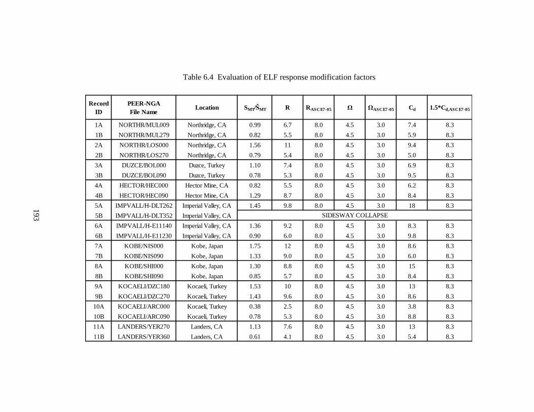
Table 6.4 Evaluation of ELF response modification factors
Record
ID
PEER-NGA
File NameLocation SMT/SMT R RASCE7-05 Ω ΩASCE7-05 Cd 1.5*Cd,ASCE7-05
1A NORTHR/MUL009 Northridge, CA 0.99 6.7 8.0 4.5 3.0 7.4 8.3
1B NORTHR/MUL279 Northridge, CA 0.82 5.5 8.0 4.5 3.0 5.9 8.3
2A NORTHR/LOS000 Northridge, CA 1.56 11 8.0 4.5 3.0 9.4 8.3
2B NORTHR/LOS270 Northridge, CA 0.79 5.4 8.0 4.5 3.0 5.0 8.3
3A DUZCE/BOL000 Duzce, Turkey 1.10 7.4 8.0 4.5 3.0 6.9 8.3
3B DUZCE/BOL090 Duzce, Turkey 0.78 5.3 8.0 4.5 3.0 9.5 8.3
4A HECTOR/HEC000 Hector Mine, CA 0.82 5.5 8.0 4.5 3.0 6.2 8.3
4B HECTOR/HEC090 Hector Mine, CA 1.29 8.7 8.0 4.5 3.0 8.4 8.3
5A IMPVALL/H-DLT262 Imperial Valley, CA 1.45 9.8 8.0 4.5 3.0 18 8.3
5B IMPVALL/H-DLT352 Imperial Valley, CA
6A IMPVALL/H-E11140 Imperial Valley, CA 1.36 9.2 8.0 4.5 3.0 8.3 8.3
6B IMPVALL/H-E11230 Imperial Valley, CA 0.90 6.0 8.0 4.5 3.0 9.8 8.3
7A KOBE/NIS000 Kobe, Japan 1.75 12 8.0 4.5 3.0 8.6 8.3
7B KOBE/NIS090 Kobe, Japan 1.33 9.0 8.0 4.5 3.0 6.0 8.3
8A KOBE/SHI000 Kobe, Japan 1.30 8.8 8.0 4.5 3.0 15 8.3
8B KOBE/SHI090 Kobe, Japan 0.85 5.7 8.0 4.5 3.0 8.4 8.3
9A KOCAELI/DZC180 Kocaeli, Turkey 1.53 10 8.0 4.5 3.0 13 8.3
9B KOCAELI/DZC270 Kocaeli, Turkey 1.43 9.6 8.0 4.5 3.0 8.6 8.3
10A KOCAELI/ARC000 Kocaeli, Turkey 0.38 2.5 8.0 4.5 3.0 3.8 8.3
10B KOCAELI/ARC090 Kocaeli, Turkey 0.78 5.3 8.0 4.5 3.0 8.8 8.3
11A LANDERS/YER270 Landers, CA 1.13 7.6 8.0 4.5 3.0 13 8.3
11B LANDERS/YER360 Landers, CA 0.61 4.1 8.0 4.5 3.0 5.4 8.3
SIDESWAY COLLAPSE
193

Table 6.4 (continued) Evaluation of ELF response modification factors
Record
ID
PEER-NGA
File NameLocation SMT/SMT R RASCE7-05 Ω ΩASCE7-05 Cd 1.5*Cd,ASCE7-05
12A LANDERS/CLW-LN Landers, CA 0.43 2.9 8.0 4.5 3.0 4.5 8.3
12B LANDERS/CLW-TR Landers, CA 0.84 5.7 8.0 4.5 3.0 5.8 8.3
13A LOMAP/CAP000 Loma Prieta, CA 1.00 6.8 8.0 4.5 3.0 12 8.3
13B LOMAP/CAP090 Loma Prieta, CA 0.52 3.5 8.0 4.5 3.0 5.7 8.3
14A LOMAP/G03000 Loma Prieta, CA 0.39 2.6 8.0 4.5 3.0 3.7 8.3
14B LOMAP/G03090 Loma Prieta, CA 1.70 11 8.0 4.5 3.0 7.8 8.3
15A MANJIL/ABBAR-L Manjil, Iran 1.45 9.8 8.0 4.5 3.0 6.9 8.3
15B MANJIL/ABBAR-T Manjil, Iran 2.27 15 8.0 4.5 3.0 8.7 8.3
16A SUPERST/B-ICC000 Superstition Hills, CA 1.14 7.7 8.0 4.5 3.0 8.1 8.3
16B SUPERST/B-ICC090 Superstition Hills, CA 1.88 13 8.0 4.5 3.0 9.6 8.3
17A SUPERST/B-POE270 Superstition Hills, CA 1.55 10 8.0 4.5 3.0 12 8.3
17B SUPERST/B-POE360 Superstition Hills, CA 1.64 11 8.0 4.5 3.0 11 8.3
18A CAPEMEND/RIO270 Cape Mendocino, CA 0.76 5.1 8.0 4.5 3.0 7.4 8.3
18B CAPEMEND/RIO360 Cape Mendocino, CA 0.40 2.7 8.0 4.5 3.0 5.1 8.3
19A CHICHI/CHY101-E Chi-Chi, Taiwan 1.08 7.3 8.0 4.5 3.0 7.4 8.3
19B CHICHI/CHY101-N Chi-Chi, Taiwan 1.59 11 8.0 4.5 3.0 9.8 8.3
20A CHICHI/TCU045-E Chi-Chi, Taiwan 0.69 4.7 8.0 4.5 3.0 7.7 8.3
20B CHICHI/TCU045-N Chi-Chi, Taiwan 0.76 5.1 8.0 4.5 3.0 8.9 8.3
21A SFERN/PEL090 San Fernando, CA 1.34 9.0 8.0 4.5 3.0 15 8.3
21B SFERN/PEL180 San Fernando, CA 1.56 11 8.0 4.5 3.0 11 8.3
22A FRIULI/A-TMZ000 Friuli, Italy 0.57 3.8 8.0 4.5 3.0 4.4 8.3
22B FRIULI/A-TMZ270 Friuli, Italy 0.51 3.4 8.0 4.5 3.0 4.1 8.3
194

Table 6.5 Frequency of drift demand exceedance
Number
of
Events
Frequency
of
Exceedance
(%)
Number
of
Events
Frequency
of
Exceedance
(%)
Number
of
Events
Frequency
of
Exceedance
(%)
Number
of
Events
Frequency
of
Exceedance
(%)
Number
of
Events
Frequency
of
Exceedance
(%)
1 6 14% 4 9% 4 9% 3 7% 2 5%
2 14 32% 7 16% 5 11% 5 11% 4 9%
3 21 48% 18 41% 11 25% 7 16% 5 11%
4 25 57% 18 41% 11 25% 10 23% 9 20%
5 14 32% 11 25% 10 23% 9 20% 5 11%
6 11 25% 9 20% 7 16% 5 11% 4 9%
7 12 27% 6 14% 5 11% 5 11% 4 9%
8 7 16% 5 11% 3 7% 2 5% 1 2%
9 3 7% 2 5% 1 2% 1 2% 1 2%
10 3 7% 2 5% 1 2% 0 0% 0 0%
IDR > 3.5%
Story
IDR > 2.5% IDR > 2.75% IDR > 3% IDR > 3.25%
195

196
Figure 6.1 Monotonic lateral load response of the test structure in the N-S direction.
Figure 6.2 Lateral load capacity and ductility.

Figure 6.3 Roof drift demand: (a) EQ1A NORTHR/MUL009; (b) EQ1B NORTHR/MUL279.
Figure 6.4 Roof drift demand: (a) EQ2A NORTHR/LOS000; (b) EQ2B NORTHR/LOS270.
197
(a) (b)
(a) (b)

Figure 6.5 Roof drift demand: (a) EQ3A DUZCE/BOL000; (b) EQ3B DUZCE/BOL090.
Figure 6.6 Roof drift demand: (a) EQ4A HECTOR/HEC000; (b) EQ4B HECTOR/HEC090.
198
(a) (b)
(a) (b)

Figure 6.7 Roof drift demand: (a) EQ5A IMPVALL/H-DLT262; (b) EQ5B IMPVALL/H-DLT352.
Figure 6.8 Roof drift demand: (a) EQ6A IMPVALL/H-E11140; (b) EQ6B IMPVALL/H-E11230.
199
(a) (b)
(a) (b)

Figure 6.9 Roof drift demand: (a) EQ7A KOBE/NIS000; (b) EQ7B KOBE/NIS090.
Figure 6.10 Roof drift demand: (a) EQ8A KOBE/SHI000; (b) EQ8B KOBE/SHI090.
200
(a) (b)
(b)
(a)

Figure 6.11 Roof drift demand: (a) EQ9A KOCAELI/DZC180; (b) EQ9B KOCAELI/DZC270.
Figure 6.12 Roof drift demand: (a) EQ10A KOCAELI/ARC000; (b) EQ10B KOCAELI/ARC090.
201
(a) (b)
(a) (b)

Figure 6.13 Roof drift demand: (a) EQ11A LANDERS/YER270; (b) EQ11B LANDERS/YER360.
Figure 6.14 Roof drift demand: (a) EQ12A LANDERS/CLW-LN; (b) EQ12B LANDERS/CLW-TR.
202
(a)
(b)
(a) (b)

Figure 6.15 Roof drift demand: (a) EQ13A LOMAP/CAP000; (b) EQ13B LOMAP/CAP090.
Figure 6.16 Roof drift demand: (a) EQ14A LOMAP/G03000; (b) EQ14B LOMAP/G03090.
203
(a) (b)
(a) (b)
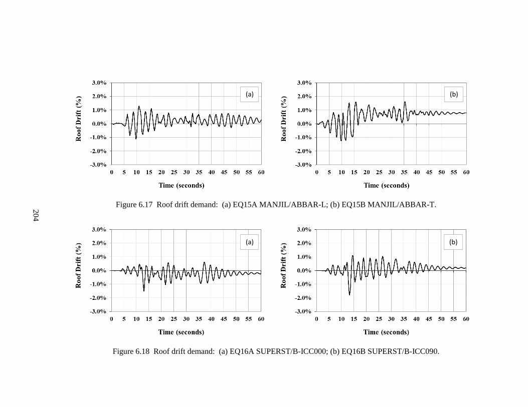
Figure 6.17 Roof drift demand: (a) EQ15A MANJIL/ABBAR-L; (b) EQ15B MANJIL/ABBAR-T.
Figure 6.18 Roof drift demand: (a) EQ16A SUPERST/B-ICC000; (b) EQ16B SUPERST/B-ICC090.
204
(a) (b)
(a) (b)

Figure 6.19 Roof drift demand: (a) EQ17A SUPERST/B-POE270; (b) EQ17B SUPERST/B-POE360.
Figure 6.20 Roof drift demand: (a) EQ18A CAPEMEND/RIO270; (b) EQ18B CAPEMEND/RIO360.
205
(a) (b)
(a) (b)

Figure 6.21 Roof drift demand: (a) EQ19A CHICHI/CHY101-E; (b) EQ19B CHICHI/CHY101-N.
Figure 6.22 Roof drift demand: (a) EQ20A CHICHI/TCU045-E; (b) EQ20B CHICHI/TCU045-N.
206
(a) (b)
(a)
(b)

Figure 6.23 Roof drift demand: (a) EQ21A SFERN/PEL090; (b) EQ21B SFERN/PEL180.
Figure 6.24 Roof drift demand: (a) EQ22A FRIULI/A-TMZ000; (b) EQ22B FRIULI/A-TMZ270.
207
(a)
(a)
(b)
(b)

Figure 6.25 Interstory drift demand: (a) EQ1A NORTHR/MUL009; (b) EQ1B NORTHR/MUL279.
Figure 6.26 Interstory drift demand: (a) EQ2A NORTHR/LOS000; (b) EQ2B NORTHR/LOS270.
208
(a) (b)
(a) (b)

Figure 6.27 Interstory drift demand: (a) EQ3A DUZCE/BOL000; (b) EQ3B DUZCE/BOL090.
Figure 6.28 Interstory drift demand: (a) EQ4A HECTOR/HEC000; (b) EQ4B HECTOR/HEC090.
209
(a) (b)
(a) (b)

Figure 6.29 Interstory drift demand: (a) EQ5A IMPVALL/H-DLT262; (b) EQ5B IMPVALL/H-DLT352.
Figure 6.30 Interstory drift demand: (a) EQ6A IMPVALL/H-E11140; (b) EQ6B IMPVALL/H-E11230.
210
(a) (b)
(a) (b)
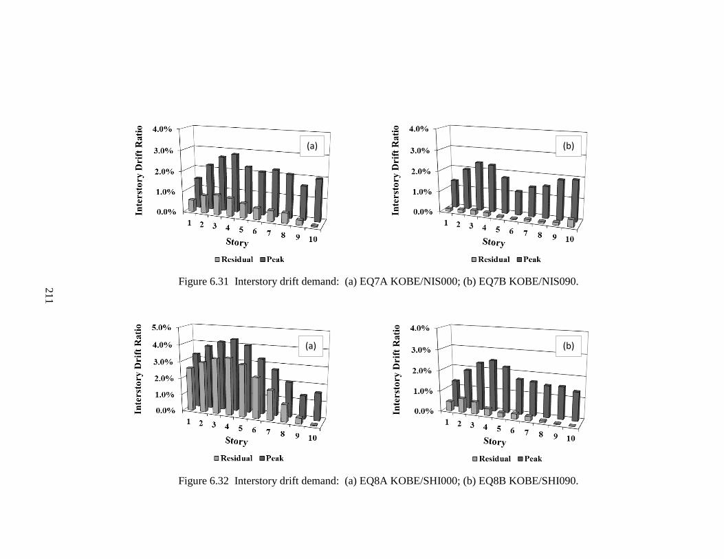
Figure 6.31 Interstory drift demand: (a) EQ7A KOBE/NIS000; (b) EQ7B KOBE/NIS090.
Figure 6.32 Interstory drift demand: (a) EQ8A KOBE/SHI000; (b) EQ8B KOBE/SHI090.
211
(a) (b)
(a) (b)

Figure 6.33 Interstory drift demand: (a) EQ9A KOCAELI/DZC180; (b) EQ9B KOCAELI/DZC270.
Figure 6.34 Interstory drift demand: (a) EQ10A KOCAELI/ARC000; (b) EQ10B KOCAELI/ARC090.
212
(a) (b)
(a) (b)
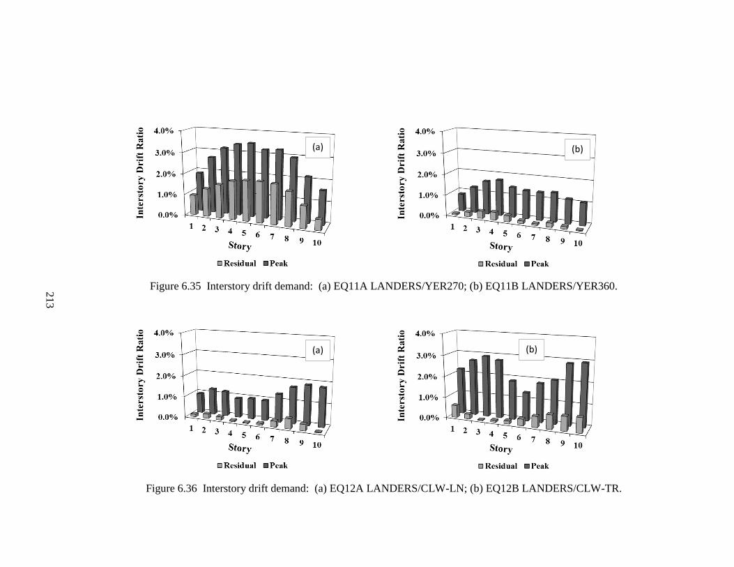
Figure 6.35 Interstory drift demand: (a) EQ11A LANDERS/YER270; (b) EQ11B LANDERS/YER360.
Figure 6.36 Interstory drift demand: (a) EQ12A LANDERS/CLW-LN; (b) EQ12B LANDERS/CLW-TR.
213
(a)
(a)
(b)
(b)

Figure 6.37 Interstory drift demand: (a) EQ13A LOMAP/CAP000; (b) EQ13B LOMAP/CAP090.
Figure 6.38 Interstory drift demand: (a) EQ14A LOMAP/G03000; (b) EQ14B LOMAP/G03090.
214
(a) (b)
(a) (b)

Figure 6.39 Interstory drift demand: (a) EQ15A MANJIL/ABBAR-L; (b) EQ15B MANJIL/ABBAR-T.
Figure 6.40 Interstory drift demand: (a) EQ16A SUPERST/B-ICC000; (b) EQ16B SUPERST/B-ICC090.
215
(a) (b)
(a) (b)

Figure 6.41 Interstory drift demand: (a) EQ17A SUPERST/B-POE270; (b) EQ17B SUPERST/B-POE360.
Figure 6.42 Interstory drift demand: (a) EQ18A CAPEMEND/RIO270; (b) EQ18B CAPEMEND/RIO360.
216
(a) (b)
(a) (b)

Figure 6.43 Interstory drift demand: (a) EQ19A CHICHI/CHY101-E; (b) EQ19B CHICHI/CHY101-N.
Figure 6.44 Interstory drift demand: (a) EQ20A CHICHI/TCU045-E; (b) EQ20B CHICHI/TCU045-N.
217
(a) (b)
(a) (b)

Figure 6.45 Interstory drift demand: (a) EQ21A SFERN/PEL090; (b) EQ21B SFERN/PEL180.
Figure 6.46 Interstory drift demand: (a) EQ22A FRIULI/A-TMZ000; (b) EQ22B FRIULI/A-TMZ270.
218
(a)
(a)
(b)
(b)

Figure 6.47 Lateral floor displacements: (a) EQ1A NORTHR/MUL009; (b) EQ1B NORTHR/MUL279.
Figure 6.48 Lateral floor displacements: (a) EQ2A NORTHR/LOS000; (b) EQ2B NORTHR/LOS270.
219
(a) (b)
(a) (b)

Figure 6.49 Lateral floor displacements: (a) EQ3A DUZCE/BOL000; (b) EQ3B DUZCE/BOL090.
Figure 6.50 Lateral floor displacements: (a) EQ4A HECTOR/HEC000; (b) EQ4B HECTOR/HEC090.
220
(a) (b)
(a) (b)

Figure 6.51 Lateral floor displacements: (a) EQ5A IMPVALL/H-DLT262; (b) EQ5B IMPVALL/H-DLT352.
Figure 6.52 Lateral floor displacements: (a) EQ6A IMPVALL/H-E11140; (b) EQ6B IMPVALL/H-E11230.
221
(a) (b)
(a) (b)

Figure 6.53 Lateral floor displacements: (a) EQ7A KOBE/NIS000; (b) EQ7B KOBE/NIS090.
Figure 6.54 Lateral floor displacements: (a) EQ8A KOBE/SHI000; (b) EQ8B KOBE/SHI090.
222
(a)
(a)
(b)
(b)

Figure 6.55 Lateral floor displacements: (a) EQ9A KOCAELI/DZC180; (b) EQ9B KOCAELI/DZC270.
Figure 6.56 Lateral floor displacements: (a) EQ10A KOCAELI/ARC000; (b) EQ10B KOCAELI/ARC090.
223
(a) (b)
(a) (b)

Figure 6.57 Lateral floor displacements: (a) EQ11A LANDERS/YER270; (b) EQ11B LANDERS/YER360.
Figure 6.58 Lateral floor displacements: (a) EQ12A LANDERS/CLW-LN; (b) EQ12B LANDERS/CLW-TR.
224
(a)
(a)
(b)
(b)

Figure 6.59 Lateral floor displacements: (a) EQ13A LOMAP/CAP000; (b) EQ13B LOMAP/CAP090.
Figure 6.60 Lateral floor displacements: (a) EQ14A LOMAP/G03000; (b) EQ14B LOMAP/G03090.
225
(a)
(a)
(b)
(b)

Figure 6.61 Lateral floor displacements: (a) EQ15A MANJIL/ABBAR-L; (b) EQ15B MANJIL/ABBAR-T.
Figure 6.62 Lateral floor displacements: (a) EQ16A SUPERST/B-ICC000; (b) EQ16B SUPERST/B-ICC090.
226
(a)
(a)
(b)
(b)

Figure 6.63 Lateral floor displacements: (a) EQ17A SUPERST/B-POE270; (b) EQ17B SUPERST/B-POE360.
Figure 6.64 Lateral floor displacements: (a) EQ18A CAPEMEND/RIO270; (b) EQ18B CAPEMEND/RIO360.
227
(a)
(a)
(b)
(b)

Figure 6.65 Lateral floor displacements: (a) EQ19A CHICHI/CHY101-E; (b) EQ19B CHICHI/CHY101-N.
Figure 6.66 Lateral floor displacements: (a) EQ20A CHICHI/TCU045-E; (b) EQ20B CHICHI/TCU045-N.
228
(a)
(a)
(b)
(b)

Figure 6.67 Lateral floor displacements: (a) EQ21A SFERN/PEL090; (b) EQ21B SFERN/PEL180.
Figure 6.68 Lateral floor displacements: (a) EQ22A FRIULI/A-TMZ000; (b) EQ22B FRIULI/A-TMZ270.
229
(a)
(a)
(b)
(b)

230
Figure 6.69 Interstory drift demand,
MCE-scaled record ensemble.
Figure 6.70 Comparison of inherent damping models -
roof drift demand for EQ11A.

231
Figure 6.71 Residual destabilizing moment at the 4
th floor,
MCE-scaled record ensemble.

232
Figure 6.72 Rotational demand in ConnC2F4 for EQ11A.
Figure 6.73 ConnC2F4 beam flange strain demands for EQ11A.

233
Figure 6.74 ConnC2F4 column flange strain demands for EQ11A.
Figure 6.75 ConnC2F4 panel zone strain demands for EQ11A.

234
Figure 6.76 Rotational demand in ConnC2F4 for EQ17A.
Figure 6.77 ConnC2F4 beam flange strain demands for EQ17A.

235
Figure 6.78 ConnC2F4 column flange strain demands for EQ17A.
Figure 6.79 ConnC2F4 panel zone strain demands for EQ17A.

236
Figure 6.80 Frequency of drift demand exceedance.

237
CHAPTER 7
THERMOMECHANICAL MOMENT-FRAME
BEAM-COLUMN CONNECTION SUBMODEL
7.1 OVERVIEW
A high-fidelity moment-frame beam-column connection submodel was developed in the
nonlinear finite element software Abaqus (Abaqus, 2011) to study transient heat flow and
thermomechanical response during post-earthquake fire exposure. In order to simplify
the thermomechanical simulation, a one-way coupling methodology was utilized, in
which an uncoupled heat transfer simulation was used to drive a dependent stress
analysis. A description of the analytical model and simulation methodology is provided
in the following sections. Section 7.2 presents the numerical model developed to
simulate heat transfer during ambient fire exposure. The coupled thermomechanical
simulation for evaluating structural response during fire exposure is discussed in Section
7.3. Section 7.4 presents the test matrix for the submodel study. Analytical results from
the submodel study are provided in Chapter 8.
7.2 HEAT TRANSFER SIMULATION
7.2.1 Analytical Components
Graphical representations of the three-dimensional finite element heat transfer model
developed for moment-frame beam-column subassemblage ConnC2F4 are presented in
Figures 7.1 and 7.2. Analytical components were developed for the steel framework
(including the web plate connection and panel zone reinforcement), SFRM insulation,

238
and a section of the concrete floor slab. Dimensional information for the subassemblage
is provided in Figure 7.3. It is noted that following idealizations were utilized to simplify
the geometry of the analytical model:
The web fillet regions of the rolled wide flange sections were neglected.
The weld access holes in the web plate, shown in Figure 3.3, were neglected.
The web connection plate geometry, shown in Figure 3.3, was idealized as a
rectangular plate.
Erection bolts and holes were neglected.
The slab on metal deck floor system was idealized as a 100mm thick concrete
slab.
Section length and tributary floor width were selected for computational efficiency
(minimization of model size), and so as to not influence the heat transfer analysis in the
beam hinge and panel zone regions, i.e. so that the artificial adiabatic boundary
conditions at the beam ends and slab edges did not influence the analytical predictions in
regions assumed to have a large relative influence on moment-rotation response of the
beam-column subassemblage. Isolated component heat transfer analyses for an insulated
beam, an insulated column, and a section of the concrete floor slab were used to verify
that the artificial adiabatic boundary conditions of the beam-column subassemblage did
not influence temperature predictions in the designated critical regions.

239
In order to facilitate compatible data transfer with the thermomechanical simulation
model, discussed further in Section 7.3, the subassemblage was subdivided into the
following component regions, or parts:
2-steel beam parts
1-steel beam-column panel zone part
2-steel column parts
2-steel web connection plate parts
2-beam SFRM insulation parts
1-panel zone SFRM insulation part
2-column SFRM insulation parts
2-web connection plate SFRM insulation parts
1-concrete floor slab part
Three dimensional solid models of the components were developed in the graphical
software package AutoCAD (AutoCAD, 2011) and were imported into the Abaqus model
workspace as 3-D deformable continuum parts. Renderings of the solid parts are
presented in Figure 7.4.
7.2.2 Analytical Mesh: Element Selection, Mesh Discretization, and Connectivity
The structural steel, SFRM insulation, and concrete floor slab parts were modeled using
an analytical mesh of 20-node quadratic continuum heat transfer elements (type DC3D20
in the Abaqus element library). The selection of element type was based on the work of
Lee et al. (2006), which found that the Abaqus DC3D20 quadratic heat transfer element

240
provided superior convergence compared to a conventional first-order h-convergence
methodology (mesh refinement by increasing the number of elements without modifying
the geometric order of the elements) when modeling temperature propagation in SFRM
insulated structural steel HSS columns. The study also found that a single quadratic heat
transfer element in the through-thickness direction provided accurate time history
predictions of temperature in the SFRM insulation and steel flanges. The analytical test
specimen for the study was a 580mm x 580mm x 4.3m steel HSS column with a flange
thickness of 40mm and an SFRM insulation thickness of 80mm. The ASTM E119
standard fire curve (Figure 2.27) was used as the ambient thermal source for the
simulation. Figures 7.5 and 7.6 present, respectively, the test matrix and numerical
results for the convergence study.
Mesh discretization for the heat transfer model was based on the aforementioned results
presented by Lee et al. (2006) and practical considerations regarding the computational
expense of the numerical simulation. The beam parts and associated SFRM insulation
were discretized with one element in the through-thickness direction, as shown in Figures
7.7 and 7.8. The thicker column sections were discretized with three elements in the
through-thickness direction of the flanges and two elements in the through-thickness
direction of the web, as shown in Figure 7.9. The SFRM insulation for the column
sections, which was thin relative to the SFRM for the beam sections due the higher
volume-to-surface area ratio, was modeled with one element in the through-thickness
direction, as shown in Figure 7.10. The analytical mesh for the beam-column panel zone
steel and SFRM insulation were discretized to match the insulated column sections, as

241
shown in Figures 7.11 and 7.12. The web connection plate was discretized with a single
element in the through thickness direction, as shown in Figure 7.13, and the associated
SFRM insulation was discretized with two elements in the through-thickness direction, as
shown in Figure 7.14, for mesh compatibility and aspect ratio considerations (discussed
later). Lastly, the concrete floor slab was discretized with two elements in the through-
thickness direction, as shown in Figure 7.15. The lower mesh refinement in the concrete
floor slab was considered reasonable since determination of temperature propagation in
the slab during fire exposure was not an objective of the study.
Mesh discretization in the longitudinal direction was based on considerations of element
aspect ratio (ratio of the longest dimension to the shortest dimension) and shape
(angularity). Large aspect ratios and/or distorted corner angles can degrade
computational accuracy of the element because they artificially bias the element shape
functions, which may result in significantly different behavior than was intended in the
element formulation.
Adjoining part interfaces were linked using the surface-based tie constraint in the Abaqus
constraint library. The surface-based tie constraint is capable of handling incompatible
meshes by transferring interpolated field data from the master surface to the nearest
geometrically positioned nodes on the slaved surface.
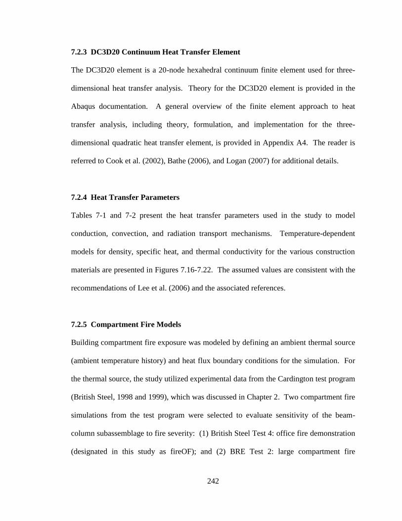
242
7.2.3 DC3D20 Continuum Heat Transfer Element
The DC3D20 element is a 20-node hexahedral continuum finite element used for three-
dimensional heat transfer analysis. Theory for the DC3D20 element is provided in the
Abaqus documentation. A general overview of the finite element approach to heat
transfer analysis, including theory, formulation, and implementation for the three-
dimensional quadratic heat transfer element, is provided in Appendix A4. The reader is
referred to Cook et al. (2002), Bathe (2006), and Logan (2007) for additional details.
7.2.4 Heat Transfer Parameters
Tables 7-1 and 7-2 present the heat transfer parameters used in the study to model
conduction, convection, and radiation transport mechanisms. Temperature-dependent
models for density, specific heat, and thermal conductivity for the various construction
materials are presented in Figures 7.16-7.22. The assumed values are consistent with the
recommendations of Lee et al. (2006) and the associated references.
7.2.5 Compartment Fire Models
Building compartment fire exposure was modeled by defining an ambient thermal source
(ambient temperature history) and heat flux boundary conditions for the simulation. For
the thermal source, the study utilized experimental data from the Cardington test program
(British Steel, 1998 and 1999), which was discussed in Chapter 2. Two compartment fire
simulations from the test program were selected to evaluate sensitivity of the beam-
column subassemblage to fire severity: (1) British Steel Test 4: office fire demonstration
(designated in this study as fireOF); and (2) BRE Test 2: large compartment fire

243
(designated in this study as fireLC). Figure 7-23(a) depicts the compartment boundaries
for the two fire simulations superimposed on the typical framing plan for the test
structure. The mean atmospheric temperature record for each fire simulation is provided
in Figure 7-23(b). For comparison, the temperature histories are plotted alongside the
ASTM E119 (ASTM, 2000a) standard fire curve.
The office fire simulation considered a 136m2 corner compartment with an equivalent
wood fuel load of 46kg/m2. The peak atmospheric temperature and 2-hour thermal load
were 921oC and 50,000
oC-min, respectively. For simplicity, a linearized version of the
temperature history (presented in Figure 7.23b) was utilized in the heat transfer analysis.
The large compartment fire simulation considered a 340m2 compartment with an
equivalent wood fuel load of 40kg/m2. The large ventilation area for this simulation
elongated the duration of the fire but produced lower temperatures compared to the office
fire simulation. The peak atmospheric temperature and 2-hour thermal load for the large
compartment fire simulation were 675oC and 57,000
oC-min, respectively.
It is noted that both compartment fire models implicitly assumed complete burnout of the
room with no intervention or active fire suppression. As has been discussed in Chapter 2,
the probability of a complete burnout scenario is significantly increased after a major
seismic event due to delayed response time for fire-fighting personal and damage to
active fire suppression systems (e.g. damage to a water supply line for an automatic
sprinkler system).

244
The numerical heat transfer simulation was executed within a single analysis step, which
was discretized into real time increments of 5min. Thermal boundary conditions for
convection and radiation transport mechanisms were introduced through the interaction
module as surface film and surface radiation conditions, respectively, on the fire exposed
and unexposed surfaces of the subassemblage. The four surface interactions utilized in
the simulation are provided below. Fire exposed and unexposed boundary surfaces, as
well adiabatic boundary surfaces, are identified in Figures 7.24 and 7.25.
Surface film condition (convection) – exposed surface
Surface radiation condition – exposed surface
Surface film condition (convection) – unexposed surface
Surface radiation condition – unexposed surface
For the convection boundary condition on the exposed surfaces, the film coefficient was
defined as an embedded parameter equal to the respective convection coefficient from
Table 7.2. This film coefficient was applied instantaneously within the analysis step.
The sink (or ambient) temperature for the simulation was specified by setting the
reference temperature to unity and the amplitude history to the time-temperature fire
model (thermal source). The analysis time history was therefore equivalent to the real-
time fire simulation.
For the radiation boundary condition on the exposed surfaces, the radiation type was set
to ambient and emissivity distribution was specified as uniform. The emissivity
245
coefficient was set to the respective value from Table 7.2, and the ambient temperature
was specified in a similar manner to the convection boundary condition.
For the convection and radiation boundary conditions on the unexposed surfaces, the
surface film coefficient (convection coefficient) and emissivity were adjusted according
to Table 7.2, and the ambient condition was set to normal ambient temperature (20oC),
which was applied instantaneously in the analysis step.
7.2.6 Damage Model for SFRM Insulation
An idealized damage model for SFRM insulation was developed based on the protected
moment-frame beam-column subassemblage tests reported by Braxtan and Pessiki (2009,
2011a, 2011b), discussed in Chapter 2 of this report. In order to simplify the analysis,
only the spalling failure mechanism was considered, although it is acknowledged that
debonding and cracking of SFRM insulation could have an effect on heat penetration into
the structural steel. The damage model used in the study considered a simple
phenomenological relationship, or fragility function, that associated an idealized damage
state (spall pattern) in the SFRM insulation with a critical peak drift angle demand in the
connection. That is, two damage states for SFRM insulation were considered: (1) an
undamaged or fully insulated case (designated in this study as sfrmPROT); and (2) an
idealized damaged state (designated in this study as sfrmDAM). Based on test
observations, a section of insulation equal to the beam flange in width and 75% of the
beam depth in length was assumed to fail (spall) along the underside of the lower beam

246
flange adjacent to the column face at a peak rotational demand, measured in terms of drift
angle, of 3%.
For the submodel heat transfer simulation, SFRM damage states sfrmPROT and
sfrmDAM were investigated. In the damaged scenario, the SFRM spall pattern was built
into the solid model for the beam SFRM insulation part, as shown in Figure 7.26.
7.2.7 Simulation Methodology and Execution
In order to simplify the analysis, the numerical heat transfer simulation was performed in
a separate model space from the thermomechanical simulation, and was, therefore, kept
independent of the mechanical stress-strain field. As a result, the heat transfer analysis
neglected the effect of element deformations on heat propagation in the model. This
approach was considered reasonable for the small deformation response range where
element deformations and displacements do not significantly impact the surface to
volume ratios for the analytical parts or create/destroy contact between elements. The job
file for the heat transfer simulation consisted of the single heat transfer analysis step
described in Section 7.2.5. Output data from the analysis was saved at a uniform step-
time interval of 300-seconds during the simulation (equivalent to real time instances for
the fire simulation). The job was executed on Lehigh University’s high performance
Linux Beowulf cluster Blaze, which contains a total of 120 64-bit AMD Opteron
processors and 2G of RAM per node, with an approximate run time of 12 hours.
247
The following files were retained for the subsequent thermomechanical simulation, as
discussed in Section 7.3.6:
output database file (.odb)
part file (.prt)
7.3 THERMOMECHANICAL SIMULATION
7.3.1 Analytical Components
A graphical representation of the thermomechanical model developed for beam-column
subassemblage ConnC2F4 is presented in Figure 7.27. For the purpose of mapping nodal
temperatures from the heat transfer simulation (discussed in Section 7.3.6), the
thermomechanical model utilized the same steel framework parts developed for the heat
transfer model. The SFRM and concrete slab were excluded from the structural portion
of the simulation. Two-dimensional beam-column elements were added through the
CAE interface to model the additional beam and column lengths for the subassemblage,
considering a beam-column subassemblage based on center-of-bay and center-of-story
dimensions. Dimensional information for the thermomechanical model is presented in
Figure 7.28.
7.3.2 Analytical Mesh: Element Selection, Mesh Discretization, and Connectivity
The beam and column hinge regions and panel zone were modeled with 20-node,
quadratic, fully-integrated, continuum stress analysis elements (type C3D20 in the
Abaqus element library), and were discretized for compatibility with the heat transfer
simulation. The use of fully-integrated quadratic stress analysis elements also ensured

248
that the continuum elements were not susceptible to the numerical problems related to
shear locking or hourglassing.
Shear locking occurs when the interpolation functions are not able to model the
deformations in the element, i.e. the element is over-constrained. Continuum elements
utilizing linear interpolation functions to calculate internal displacements are only
capable of modeling uniform strain, and are therefore unable to model a strain gradient,
i.e. flexural response. This phenomenon is known as shear locking because the
interpolation functions force the element into a shear mode of response (Figure 7.28),
giving rise to large artificial shear strains. The end result is that the stiffness of the
element in bending can be significantly overestimated.
Hourglassing can occur in continuum elements that utilize a single-point reduced
integration scheme. While a reduced integration approach can significantly improve the
computational cost of a numerical simulation, it also makes the element susceptible to the
zero energy shear deformation mode shown in Figure 7.29 because strain demands are
only monitored along the neutral axis.
For computational efficiency, the beam and column extensions were modeled with
nonlinear, distributed plasticity, cubic-formulation, beam-column elements (type B33 in
the Abaqus element library). Multi-point kinematic constraints were used to enforce
compatibility at the linear element-to-continuum element transitions (Figure 7.31). This
approach used a kinematic constraint law to slave the nodal translations on the

249
connecting surface of the continuum body to the nodal displacements of the connecting
beam node (designated as the control node). The constraint considered the respective
eccentricity between the control node and the slaved node and was therefore capable of
transferring translational and rotational displacements.
Surface-based tie constraints were used to mechanically join the connecting surfaces of
the continuum element assembly. This approach was similar to the method utilized in the
heat transfer model.
7.3.3 C3D20 Continuum Stress Analysis Element
The C3D20 element is a 20-node quadratic hexahedral continuum finite element used for
three-dimensional stress analysis. Theory for the C3D20 element is provided in the
Abaqus documentation. A general overview of the finite element approach to continuum
stress analysis, including theory, formulation, and implantation for the three-dimensional
quadratic heat transfer element, is provided in Appendix A5. The reader is referred to
Cook et al. (2002), Bathe (2006), and Logan (2007) for additional details.
7.3.4 Material Model
The nonlinear stress-strain response model for structural steel was developed using the
temperature-dependent models for elastic modulus and yield stress presented in EC3
(BSI, 2001), which are shown graphically in Figure 7.32. The baseline stress-strain
response at normal ambient temperature was based on the idealized bi-linear backbone
curve and kinematic hardening model presented in Figures 4.3 and 4.4. Post-yield

250
response in the elevated temperature range was based on a consistent strain hardening
ratio of 1%.
7.3.5 Mechanical Boundary Conditions
In order to study the influence of in-situ mechanical boundary conditions on response of
the beam-column subassemblage during fire exposure, three idealized models were
developed for the adjoining framework: (1) a flexible restraint model (designated as
expFLEX); (2) a free expansion model (designated as expFREE); and (3) a fully
restrained model (designated as expRES). The free expansion and fully restrained
models were developed to bound the problem by considering idealized scenarios where
the adjoining structure either fully accommodates or fully restrains thermal expansion of
the beam-column subassemblage. The flexible restraint model was developed to provide
a more realistic estimate of in-situ mechanical restraint. For this approach, finite element
models were developed for the adjoining framework on either side of the beam-column
subassemblage using nonlinear, distributed plasticity, cubic-formulation, beam-column
elements (type B33 in the Abaqus element library). Centerline member dimensions were
utilized in order to approximate panel zone flexibility. A series of displacement-
controlled analyses, in the axial direction of the beam, were then used to evaluate force-
displacement relations for the frames, and the response data was used to calibrate
nonlinear spring supports for the submodel boundaries. Temperature effects in the
surrounding framework were considered based on the limits of the assumed fire
compartment. The North and South framework models included the adjacent SMF
beams along the 4th
elevated floor as well as the 4th
and 5th
story SMF columns (full story

251
height). The ends of the columns were assumed to be fully restrained by the connecting
beams, i.e. fixed boundary conditions. Figures 7.33 and 7.35 present the finite element
models developed for the North and South framework, respectively. The corresponding
force-displacement response curves for imposed translation along the beam axis are
presented in Figures 7.34 and 7.36.
As previously discussed, the composite floor slab was excluded from the mechanical
simulation in order to simplify the analysis. The lateral restraint provided by the floor
slab, however, was implicitly included by restraining the upper flange of the continuum
beam parts (outside of the protected hinge region) and the beam extensions for lateral
motion, as shown in Figure 7.27.
7.3.6 Simulation Methodology and Execution
As discussed in Section 7.2.7, the thermomechanical simulation model was developed in
a separate model space from the heat transfer analysis. A multi-step sequential analysis
procedure was developed to simulate seismic response in the beam-column
subassemblage and subsequent thermal loading during post-earthquake fire exposure.
The procedure was designed to transfer the residual stress/strain field from the previous
analysis step to the next in order to capture the effect of residual deformations and stress
demands on structural response during ambient thermal heating. It is noted that the
analysis did not consider the residual stress demands in the steel sections due to
fabrication. These stresses were thought to be less important in the critical heat-affected
regions (where localized response has the highest impact on moment-rotation response of

252
the beam-column subassemblage) since the elevated steel temperatures during the fire
simulation effectively anneal the residual stress field (Buchanan, 2002). In addition, the
effect of fabrication-related stress demands on the driving forces in the heat-affected
region was thought to be small relative to force demands in the damaged building due to
residual second-order destabilizing loads and/or locked-in forces due to residual inelastic
deformations.
7.3.6.1 Phase 1 - Earthquake Simulation
The first phase of the analysis utilized a series of sequential static analysis steps to
simulate seismic response in the beam-column subassemblage in order to develop the
residual stress/strain field. This was accomplished by imposing nodal displacement
histories from the dynamic analyses of Chapter 6 at the respective boundary nodes. The
procedure is shown schematically in Figure 7.37. The imposed drift angle history for the
earthquake simulation was based on the EQ11A-ConnC2F4 response record, discussed in
Section 6.8. For simplicity, the EQ11A-ConnC2F4 record was idealized by linearizing
the response between local peaks in rotational demand. The recorded and linearized
EQ11A-ConnC2F4 response records are plotted in Figure 7.38.
It is noted that good agreement was found in the monotonic and cyclic response of the
fiber element beam-column connection model utilized in the dynamic analyses of
Chapter 6 and the high-fidelity continuum finite element beam-column submodel,
developed in this chapter, for interstory drift demands up to approximately 3%, as shown
in Figures 7.39 and 7.40. For interstory drift demands larger than 3%, buckling

253
distortions in the beam hinge region of the high-fidelity submodel caused geometric
softening of moment-rotation response for the assembly. Figure 7.41 presents the
buckling distortions and plastic strain distribution in the beam hinge region at a drift
demand of 3.5%. It was noted in Chapter 4 that these buckling distortions are not
modeled by the fiber element, and, as a result, the moment-rotation response of the two
beam-column subassemblage models begins to diverge. However, since rotational
demands in ConnC2F4 for the selected MCE event are within the range of closely
correlated response, the transfer of deformation demands from the dynamic system model
to the continuum beam-column submodel is considered reasonable.
7.3.6.2 Phase 2A – Post-Earthquake Fire Simulation
The second phase of the analysis involved simulating post-earthquake fire exposure and
investigating the effects of temperature-induced softening and restrained thermal
expansion under the action of the residual force system. To accomplish this task, a series
of sequential stress analyses were performed utilizing the temporal-spatial nodal
temperature data from the uncoupled heat transfer simulation. The procedure is shown
schematically in Figure 7.42. At selected time instances during the fire simulation
(20min, 40min, and 60min), nodal temperatures were imported as field data into the
stress analysis model. The selection of time instances was based on recorded steel
temperatures and was intended to characterize the heating phase of the fire, particularly
the peak steel temperatures. For the continuum parts, nodal temperatures were imported
directly from the heat transfer simulation output database file as a predefined temperature
field, referencing the respective output database file name, analysis step, and step-time

254
instance. Temperatures for the beam and column extensions were directly specified at
five section integration points (as shown in Figure 7.42) based on recorded temperature
profiles from the heat transfer simulations.
In order to establish a consistent baseline force system between test cases, the residual
(post-earthquake) moment demand in the connection was held constant during the fire
simulation. This was accomplished by releasing the vertical restraint at the beam control
nodes, and applying the lost reaction forces as concentrated loads. A series of static
analysis steps were then performed, sequentially, at each of the selected time instances
during the fire simulation to determine the new state of equilibrium, considering both
temperature-induced material softening and thermal distortion. It is noted that actual
force demands on the beam-column subassemblage could change significantly during fire
exposure due to load redistribution and/or the presence of stabilizing or destabilizing
forces in the structural system
7.3.6.3 Phase 2B – Displacement-Controlled Analyses
For each of the selected time instances during the fire simulation, monotonic
displacement-controlled analyses were used evaluate the effect of heat propagation on
moment-rotation response, i.e. to determine the moment-rotation response of the heat-
affected beam-column subassemblage independent of the external force demand. These
analyses were performed in a series of static analysis steps using imposed translational
nodal displacements. The procedure is shown schematically in Figure 7.43. The beam
control nodes were restrained for translational displacements (pinned) at the final

255
deformed position for the selected time instance. The horizontal coordinates of the upper
and lower column control nodes were then adjusted anti-symmetrically in order to impose
a progressively increasing drift demand in the connection.
Since the Phase 2B displacement-controlled analyses were performed at specific time
instances during the fire simulation (20min, 40min, and 60min), requiring the termination
of the Phase 2A simulation at the time instance of interest, three separate CAE model
files were developed. As previously noted, the Phase 2A simulations for the latter time
instances (40min and 60min) included step(s) for the previous time instance(s).
7.3.6.4 Analysis Restart Procedure
Due to limitations with accessing output database files larger than 2GB on a standard
personal computer, an analysis restart procedure was utilized to separate the
thermomechanical simulation into two phases, thereby segregating the output data into
two separate output database files. The break in the simulation was positioned at the end
of the earthquake simulation. The procedure for restarting the simulation required the
following steps:
A restart request was added to the final analysis step of the Phase 1 - earthquake
simulation model through the load module in the CAE GUI. This step added coding
to the job input file to generate the analysis restart file (.res).
The Phase 2 – post-earthquake fire simulation model was then created by copying the
Phase 1 model to a new workspace. The model attribute editor was used to point the
Phase 2 model to the job file from the Phase 1 simulation, indicating the specific

256
analysis step and step-time instance. As discussed previously, separate Phase 2
models were developed for each time instance in order perform the Phase 2B
pushover analyses.
In order to restart the analysis and execute the Phase 2 simulations, the following
files were located and referenced in the job directory:
Output database file from heat transfer simulation (.odb)
Part file from heat transfer simulation (.prt)
Output database file from Phase 1-earthquake simulation (.odb)
Part file from Phase 1-earthquake simulation (.prt)
Restart file from Phase 1-earthquake simulation (.res)
State file from Phase 1-earthquake simulation (stt)
Model file from Phase 1-earthquake simulation (.mdl)
7.4 TEST MATRIX
A summary of the test matrix for the study is provided in Table 7.3. Nine test scenarios
were developed to consider two SFRM damage states (sfrmPROT and sfrmDAM), three
ambient exposure conditions (No Fire, fireOF, and fireLC), and three in-situ boundary
condition models (expFREE, expRES, expFLEX). Scenarios 1-5 were used to evaluate
the effect of the SFRM damage on heat penetration into the structural steel and
temperature-induced degradation of moment-rotation response for the beam-column
subassemblage. The influence of in-situ boundary restraint against thermal expansion
was considered in a comparative study of Scenarios 2, 3, 6-9.

257
7.5 SUMMARY
A high-fidelity moment-frame beam-column connection submodel was developed in the
nonlinear finite element software Abaqus to study transient heat flow and
thermomechanical response during post-earthquake fire exposure. In order to simplify
the thermomechanical simulation, a one-way coupling methodology was utilized, in
which an uncoupled heat transfer simulation was used to drive a dependent stress
analysis. Compartment fire models were developed from large-scale fire tests and
available literature regarding heat flux boundary conditions. An idealized damage model
for SFRM insulation in moment-frame beam hinge regions was developed from
experimental test data. In-situ mechanical boundary condition models were developed to
evaluate the influence of restrained thermal expansion on moment-rotation response of
the beam-column assembly during fire exposure. The test matrix for the submodel study
considered two SFRM damage states, three fire exposure conditions, and three in-situ
mechanical boundary condition models.

Table 7.1 Conductive heat transfer properties
Table 7.2 Heat flux boundary conditions
A992 Steel 7850 Figure 7.16 Figure 7.17 (BSI, 2001)
Dry-Mix SFRM Figure 7.18 Figure 7.19 Figure 7.20 NIST (2005)
Normal Wt.
Concrete2300 Figure 7.21 Figure 7.22 (BSI, 1996)
MaterialDensity, ρ
(kg/m3)
Specific Heat, cp
[J/(kg-K)]
Thermal
Conductivity, k
[W/(m-K)]
Reference
Exposed Surface Unexposed Surface Exposed Surface Unexposed Surface
25 10 1.0 1.0 (SFPE, 2004)
Reference
Convection Coefficient, h
[W/(m2-K)]Resultant Emissivity, εr
258
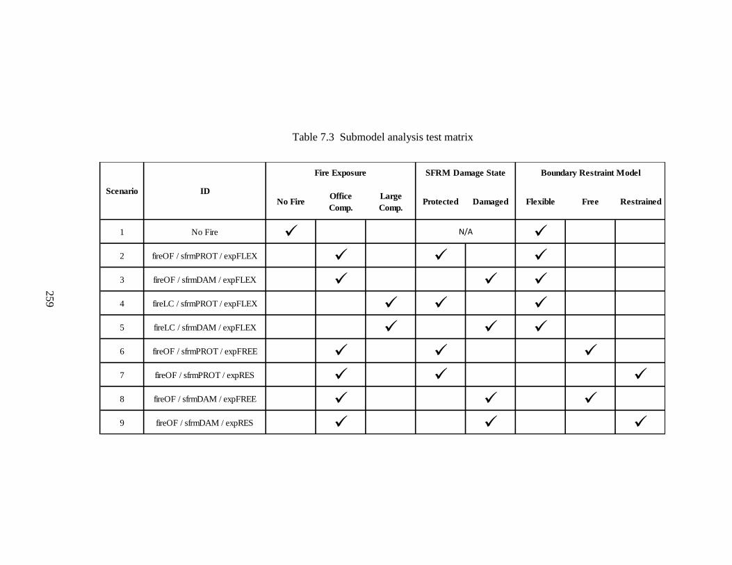
Table 7.3 Submodel analysis test matrix
No FireOffice
Comp.
Large
Comp.Protected Damaged Flexible Free Restrained
1 No Fire
2 fireOF / sfrmPROT / expFLEX
3 fireOF / sfrmDAM / expFLEX
4 fireLC / sfrmPROT / expFLEX
5 fireLC / sfrmDAM / expFLEX
6 fireOF / sfrmPROT / expFREE
7 fireOF / sfrmPROT / expRES
8 fireOF / sfrmDAM / expFREE
9 fireOF / sfrmDAM / expRES
Boundary Restraint Model
N/A
Scenario ID
Fire Exposure SFRM Damage State
259

260
Figure 7.1 Finite element heat transfer model for ConnC2F4
(model with SFRM damage shown).
Figure 7.2 Finite element heat transfer model for ConnC2F4
(SFRM and concrete slab removed from view).

261
(a)
(b)
Figure 7.3 Finite element heat transfer model for ConnC2F4 – detail:
(a) beam-column subassemblage; (b) panel zone.

262
(a) (b)
(c) (d) (e) (f)
(g) (h) (i) (j)
Figure 7.4 Finite element heat transfer model for ConnC2F4 – analytical parts:
(a) beam-column subassemblage; (b) concrete slab part; (c) typical beam part;
(d) panel zone part; (e) typical column part; (f) typical web connection plate
part; (g) typical beam SFRM insulation part; (h) typical column SFRM insulation
part; (i) typical column SFRM insulation part; (j) typical web connection plate
SFRM insulation part.

263
Figure 7.5 Lee et al. (2006) heat transfer analysis convergence study - test matrix.

264
Figure 7.6 Lee et al. (2006) heat transfer analysis convergence study – results.

265
Figure 7.7 Beam part mesh discretization - heat transfer simulation.
Figure 7.8 Beam SFRM insulation part mesh discretization
(model with SFRM damage shown) - heat transfer simulation.

266
Figure 7.9 Column part mesh discretization - heat transfer simulation.
Figure 7.10 Column SFRM insulation part mesh discretization - heat transfer simulation.

267
Figure 7.11 Panel zone mesh discretization - heat transfer simulation.
Figure 7.12 Panel zone SFRM insulation mesh discretization - heat transfer simulation.

268
Figure 7.13 Web connection plate mesh discretization - heat transfer simulation.
Figure 7.14 Web connection plate SFRM insulation mesh discretization
- heat transfer simulation.

269
Figure 7.15 Concrete slab mesh discretization - heat transfer simulation.
Figure 7.16 Temperature-dependent model for
specific heat of A992 steel based on EC3 (BSI, 2001).

270
Figure 7.17 Temperature-dependent model for thermal
conductivity of A992 steel based on EC3 (BSI, 2001).
Figure 7.18 Temperature-dependent model for mass
density of dry-mix SFRM based on NIST (2005).

271
Figure 7.19 Temperature-dependent model for specific
heat of dry-mix SFRM based on NIST (2005).
Figure 7.20 Temperature-dependent model for thermal
conductivity of dry-mix SFRM based on NIST (2005).

272
Figure 7.21 Temperature-dependent model for
specific heat of concrete based on EC2 (BSI, 1996).
Figure 7.22 Temperature-dependent model for thermal
conductivity of concrete based on EC2 (BSI, 1996).

273
Figure 7.23 Compartment fire models: (a) compartment boundaries;
(b) mean atmospheric temperature records.
(a)
(b)
(b)

274
Figure 7.24 Fire exposed surfaces - heat transfer simulation.
Figure 7.25 Unexposed surface - heat transfer simulation.
Fire
Exposed
Surfaces
Unexposed
Surface
Adiabatic
Surfaces
Adiabatic
Surfaces
Adiabatic
Surface
Adiabatic
Surface

275
Figure 7.26 Idealized SFRM spall pattern - heat transfer simulation.
Figure 7.27 Thermomechanical finite element model for ConnC2F4.
63cm x 29cm
SFRM Spall
63cm x 29cm
SFRM Spall
Distributed Restraint
for Lateral Translation
Point Restraint
for Twist

Figure 7.28 Thermomechanical finite element model for ConnC2F4 – detail.
276

277
Figure 7.29 Shear locking: (a) ideal deformed shape of a brick element under moment
demand; (b) deformed shape of first order fully integrated brick element under moment
demand; (c) deformed shape of quadratic fully integrated brick element under moment
demand
Figure 7.30 Hourglassing – deformed shape of a brick element with
single-point reduced integration under moment demand.

278
Figure 7.31 Multi-point kinematic constraint at the linear element-to-continuum
element transitions - thermomechanical simulation.
Figure 7.32 Temperature-dependent model for elastic modulus and yield stress of
structural steel based on EC3 (BSI, 2001) - thermomechanical simulation.
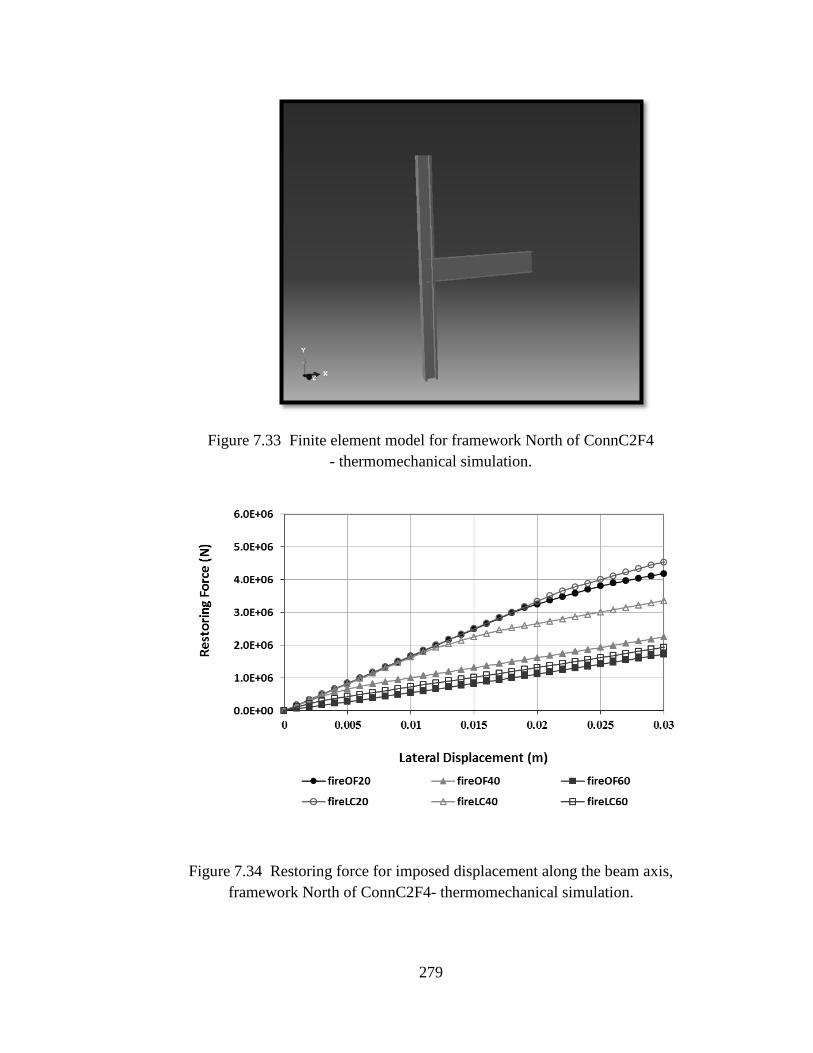
279
Figure 7.33 Finite element model for framework North of ConnC2F4
- thermomechanical simulation.
Figure 7.34 Restoring force for imposed displacement along the beam axis,
framework North of ConnC2F4- thermomechanical simulation.

280
Figure 7.35 Finite element model for framework South of ConnC2F4
- thermomechanical simulation.
Figure 7.36 Restoring force for imposed displacement along the beam axis,
framework South of ConnC2F4- thermomechanical simulation.

281
Figure 7.37 Phase 1 – earthquake simulation
Figure 7.38 Linearized ConnC2F4-EQ11A deformation history

282
Figure 7.39 ConnC2F4 submodel - monotonic moment-rotation response
Figure 7.40 ConnC2F4 submodel - cyclic moment-rotation response
(ConnC2F4-EQ11A deformation history)

283
Figure 7.41 ConnC2F4 submodel – buckling distortions and plastic strain
at a drift demand of 3.5% (deformation scale factor: x2)
(ConnC2F4-EQ11A deformation history).

284
Figure 7.42 Phase 2A – post-earthquake fire simulation.
Figure 7.43 Phase 2B – displacement-controlled (pushover) analysis.

285
CHAPTER 8
THERMOMECHANCIAL MOMENT-FRAME BEAM-COLUMN
CONNECTION SUBMODEL – ANALYTICAL RESULTS
8.1 OVERVIEW
This chapter presents results from thermomechanical post-earthquake fire simulations
utilizing the beam-column connection submodel developed in Chapter 7. Sections 8.2.1
and 8.2.2 present steel temperature recordings and temperature-adjusted material
properties for the office fire (fireOF) and large compartment fire (fireLC) simulations,
respectively. Results from the coupled thermomechanical study are presented in Section
8.3 for the office fire (Section 8.3.1) and large compartment fire (Section 8.3.2)
simulations. A discussion of the findings from the study is provided in Section 8.3.3.
The influence of mechanical restraint against thermal expansion is evaluated in Section
8.3.4.
8.2 HEAT TRANSFER SIMULATION
The following sections present results from the numerical heat transfer simulations
discussed in Section 7.2. Recorder locations for the beam-column submodel are
presented in Figure 8.1. Recorders R1, R2, and R3 are located at 32cm from the face of
the column, near the mid-length of the assumed spall in the spray-applied fire-resistive
material (SFRM). Recorder R1 is located at the mid-thickness of the upper beam flange,
near the midpoint of the outstanding flange leg. Recorder R2 is located at the mid-
thickness of the lower fire-exposed beam flange, and is also located near the midpoint of

286
the outstanding flange leg. Recorder R3 is located at the mid-thickness of the beam web,
at a distance of 22cm from the bottom of the beam section (3/4-depth). Recorder R4 is
located at the mid-width and mid-thickness of the web connection plate, at distance 22cm
from the bottom of the beam section. Finally, Recorder R5 is located at the mid-
thickness of the column flange, near the welded beam flange-to-column flange interface.
8.2.1 Office Fire Simulation
Figures 8.2-8.4 present time history recordings of steel temperature, elastic modulus, and
effective yield stress for ConnC2F4 submodels with damaged (sfrmDAM) and
undamaged (sfrmPROT) thermal insulation subjected to the office fire (fireOF)
simulation. The results are summarized in Tables 8.1 and 8.2. The temperature
recordings in Figure 8.2 illustrate that steel temperatures in the exposed, or unprotected,
region of the bottom flange in the damaged model (measured at R2) track closely with
the ambient temperature history. The ambient temperature is within 10% of its peak
value of 872oC between 15-35min, while the steel temperature at R2 is within 10% of its
peak value of 729oC between 25-55min. The associated lag time between the ambient
temperature range within 10% of the peak value and the steel temperature range within
10% of the peak value is approximately 10min.
As the ambient temperature rapidly falls between 40min and 120min into the simulation,
the steel temperature at R2 in the damaged model also declines at a similar rate. This can
be attributed to heat loss in the flange section through conductive heat transfer to cooler

287
regions of the steel beam, as well as conductive and radiative heat transfer to the cooling
ambient environment through the exposed surface (unprotected steel).
As shown in Figure 8.2, steel temperatures away from the exposed steel, in the damaged
model, rise slowly until approximately 60min into the simulation, at which point they
gradually taper off. This is attributed to the SFRM insulation retarding the rate of heating
and cooling in the protected steel, i.e. the influx of heat is slower to reach the protected
steel and slower to leave the protected steel (with respect to the exposed surface) due to
the insulated thermal boundary. As a result, thermal degradation in the beam hinge
region of the damaged model is considerably localized in the exposed flange, with only
moderate temperature-induced degradation of the elastic modulus in the adjacent beam
web (measured at R3), as shown in Figures 8.3 and 8.4. The elastic modulus of the web
connection plate (measured at R4) and column flange (measured at R5) in the damaged
model remains within 20% of its value at normal ambient temperature. The upper beam
flange is relatively unaffected by the SFRM damage. A detailed account of temperature
propagation and thermal degradation at the selected time points (20min, 40min, and
60min) is provided in the following paragraphs.
At 20min into the office fire simulation, steel temperatures in the exposed beam flanges
of the damaged submodel (measured at R2) reach 612oC, and the elastic modulus and
yield stress of the heat-affected steel are reduced to 29% and 44%, respectively, of their
values at normal ambient temperature (approximately 20oC). For convenience, these
temperature-adjusted values are expressed as a fraction of their value at 20oC, i.e. kE,T of
0.29 and kY,T of 0.44, where kE,T and kY,T represent the ratios for elastic modulus and

288
yield stress, respectively. The temperature-adjusted values for elastic modulus and yield
stress in the damaged submodel are 71% and 56% lower, respectively, than the
corresponding values for the fully insulated case. Heat penetration into the damaged
submodel is localized near the exposed flanges and only marginal increases in steel
temperature are observed in the upper beam flange (R1), beam web (R3), web connection
plate (R4), and column flange (R5).
At 40min into the office fire simulation, steel temperatures in the exposed beam flanges
of the damaged submodel near their peak value of 729oC, where kE,T and kY,T drop to 0.12
and 0.20, respectively. The steel temperature contour plot for the damaged submodel at
40min is presented Figure 8.1. Temperatures in the lower quarter of the beam web reach
335oC, where kE,T is reduced to 0.77. Steel temperatures in the upper beam flange, web
connection plate, and column flange, however, remain low enough so as to not induce
appreciable degradation of the structural steel. For the fully insulated case, steel
temperatures in the beam-column subassemblage remain below 250oC, with associated
reductions in elastic modulus of 10-15% and negligible reductions in yield stress.
At 60min into the office fire simulation, steel temperatures in the exposed beam flanges
of the damaged submodel drop to 604oC and there is marginal recovery of elastic
modulus and yield stress (kE,T = 0.30 and kY,T = 0.46). Away from the exposed surface,
steel temperatures continue to rise as a result of greater time lag between conductive heat
flow and input from the thermal source, primarily related to retarded heat flow through
the SFRM insulation. The lower quarter of the beam web reaches 413oC, where kE,T

289
drops to 0.69. Steel temperatures in the web connection plate and column flange
approach 250-280oC where kE,T is reduced to 0.85-0.82. For the fully insulated case,
steel temperatures in the lower beam flange and adjacent beam web reach 260-280oC
where kE,T is reduced to 0.84-0.82.
Between 60min and 120min during the office fire simulation, steel temperatures in the
exposed beam flanges of the damaged submodel decay rapidly from 604oC to 192
oC (-
6.9oC/min) and there is significant recovery of elastic modulus and yield stress (kE,T =
0.91 and kY,T = 1.00). The adjacent beam web, web connection plate, and column flange
also cool, but at a substantially slower rate than the exposed flanges (-0.1 to 2.0oC/min),
which can be attributed to the intact SFRM insulation impeding heat transfer to the cooler
ambient environment. The same observation applies to the fully insulated case, where
steel temperatures decay slowly during the cooling phase of the fire. As an example,
steel temperatures in the lower flange of the fully insulated submodel drop approximately
31oC from their peak at 80min during the fire simulation to 242
oC at 120min (-
0.8oC/min).
8.2.2 Large Compartment Fire Simulation
Figures 8.5-8.7 present time history recordings of steel temperature, elastic modulus, and
effective yield stress for ConnC2F4 submodels with damaged (sfrmDAM) and
undamaged (sfrmPROT) thermal insulation subjected to the large compartment fire
(fireLC) simulation. The temperature recordings in Figure 8.5 illustrate that steel
temperatures in the exposed, or unprotected, region of the bottom flange in the damaged

290
model (measured at R2) track closely with the ambient temperature history. The ambient
temperature is within 10% of its peak value of 670oC between 20-70min, while the steel
temperature at R2 is within 10% of its peak value of 618oC between 40-75min. The
associated lag time between the ambient temperature range within 10% of the peak value
and the steel temperature range within 10% of the peak value is approximately 20min.
As the ambient temperature falls between 70min and 120min into the simulation, the steel
temperature at R2 in the damaged model also declines at a similar rate, attributed to heat
loss in the flange section through conductive heat transfer to cooler regions of the steel
beam, as well as conductive and radiative heat transfer to the cooling ambient
environment through the exposed surface (unprotected steel).
As shown in Figure 8.2, steel temperatures away from the exposed steel, in the damaged
model, rise slowly until approximately 100-120min into the simulation. This is attributed
to the SFRM insulation retarding the rate of heating and cooling in the protected steel.
As a result, thermal degradation in the beam hinge region of the damaged model is
considerably localized in the exposed flange, with only moderate temperature-induced
degradation of the elastic modulus in the adjacent beam web (measured at R3), as shown
in Figures 8.6 and 8.7. The elastic modulus of the web connection plate (measured at R4)
and column flange (measured at R5) in the damaged model remains within 20% of its
value at normal ambient temperature. The upper beam flange is relatively unaffected by
the SFRM damage. A detailed account of temperature propagation and thermal

291
degradation at the selected time points (20min, 40min, and 60min) is provided in the
following paragraphs.
At 20min into the large compartment fire simulation, steel temperatures in the exposed
beam flanges of the damaged submodel reach 355oC, where kE,T is reduced to 0.74 (26%
lower than the fully insulated case). Similar to the office fire simulation, heat penetration
into the damaged submodel is localized near the exposed flanges and only marginal
increases are observed in steel temperatures for the upper beam flange, beam web, web
connection plate, and column flange.
At 40min into the large compartment fire simulation, steel temperatures in the exposed
beam flanges of the damaged submodel reach 562oC, and kE,T and kY,T drop to 0.42 and
0.59, respectively. Steel temperatures in the lower quarter of the beam web reach 222oC,
where kE,T is reduced to 0.88. Steel temperatures in the upper beam flange, web
connection plate, and column flange, however, remain low enough so as to not induce
appreciable degradation of the structural steel. For the fully insulated case, steel
temperatures remain below 150oC with negligible reduction to elastic modulus and yield
stress.
At 60min into the large compartment fire simulation, steel temperatures in the exposed
beam flanges of the damaged submodel near their peak value of 618oC, where kE,T and
kY,T drop to 0.28 and 0.43, respectively. Steel temperatures in the beam web, web
connection plate, and column flange reach 329oC, 212
oC, and 201
oC, respectively, which

292
correspond to kE,T of 0.77, 0.89,and 0.90. For the fully insulated case, steel temperatures
in the lower beam flange and adjacent beam web reach 205-227oC, where kE,T is reduced
to 0.90-0.87.
Between 60min and 120min during the large compartment fire simulation, steel
temperatures in the exposed beam flanges of the damaged submodel decay rapidly from
618oC to 318
oC (rate of -5.0
oC/min) and there is significant recovery of elastic modulus
and yield stress (kE,T = 0.78 and kY,T = 1.00). Due to the longer sustained heating phase
of the fire, steel temperatures in the adjacent beam web, web connection plate, and
column flange gradually rise to their peak at approximately 90min into the simulation,
after which they experience a gradual decay with declining ambient temperature.
8.3 THERMOMECHANICAL SIMULATION
8.3.1 Office Fire Simulation
Figure 8.8 presents moment-rotation response curves for ConnC2F4 submodels with
damaged (sfrmDAM) and undamaged (sfrmPROT) thermal insulation at 20, 40, and
60min into the office fire (fireOF). For comparison, the response curves are plotted
alongside the probable flexural strength of the beam hinge regions (Mpr,beam) and the peak
flexural resistance measured during seismic response for the EQ11A ground motion
record (Mr,peak-EQ11A). Results from the study are summarized in Table 8.3 as fractions
of the response at normal ambient temperature. As previously discussed, the residual
force demands at the end of the earthquake simulation were used as the baseline force
system for the analyses, although it is noted that actual force demands in the connection
could change significantly during the fire simulation due to load redistribution and/or the

293
presence of stabilizing or destabilizing forces. The submodel boundary conditions were
based on the flexible restraint model (expFLEX).
At 20min into the office fire simulation, the drift angle in both the fully insulated and
damaged submodels is essentially unchanged from the post-earthquake configuration
under the action of the residual force system. Under continued loading to larger
rotational demands, however, the damaged submodel exhibits softer moment-rotation
response and reduced flexural capacity. Secant rotational stiffness for the damaged
model is reduced by 27% for an additional 1% imposed drift demand and is reduced by
20% for an additional 2% imposed drift demand. Flexural capacity for the damaged
model is reduced by 17% compared to the fully insulated case.
At 40min into the office fire simulation, steel temperatures in the exposed beam flanges
of the damaged submodel near their peak. The drift angle in the fully insulated submodel
remains unchanged, but the damaged submodel propagates from 1.9% to 2.0% under the
action of the residual force system. Secant rotational stiffness for the damaged model is
reduced by 42% for additional imposed drift demands of 1% and 2%, and flexural
capacity is reduced 33% compared with the fully insulated case.
At 60min into the office fire simulation, steel temperatures for the fully insulated
submodel near their peak. Secant rotational stiffness for additional imposed drift
demands of 1% and 2% are reduced by 18% and 9%, respectively, but flexural capacity
of the connection is essentially unaffected. For the damaged submodel, steel

294
temperatures in the exposed beam flanges drop from their peak values near 40min, and
the flexural capacity rebounds to 22% of the value at normal ambient temperature.
8.3.2 Large Compartment Fire Simulation
Figure 8.9 presents moment-rotation response curves for ConnC2F4 submodels with
damaged (sfrmDAM) and undamaged (sfrmPROT) thermal insulation at 20, 40, and
60min into the large compartment fire simulation (fireOF).
At 20min into the large fire simulation, the drift angle in both the fully insulated and
damaged submodels is essentially unchanged from the post-earthquake configuration
under the action of the residual force system. Under continued loading to larger
rotational demands, however, the damaged submodel exhibits softer moment-rotation
response and reduced flexural capacity. Secant rotational stiffness for the damaged
model is reduced by 9% for an additional 1% imposed drift demand and is reduced by 1%
for an additional 2% imposed drift demand. Flexural capacity for the damaged model is
reduced by 1% compared to the fully insulated case.
At 40min into the office fire simulation, the drift angle in the fully insulated and damaged
submodels, remains unchanged under the action of the residual force system. Secant
rotational stiffness for the damaged submodel is reduced by 20% and 14% for additional
imposed drift demands of 1% and 2%, respectively, and flexural capacity is reduced 12%
compared with the fully insulated case.

295
At 60min into the office fire simulation, steel temperatures for the fully insulated and
damaged submodels near their peak. Secant rotational stiffness for the damaged
submodel is reduced by 26% and 25% for additional imposed drift demands of 1% and
2%, respectively, and flexural capacity is reduced by 21% compared to the fully insulated
case.
8.3.3 Comparison of Protected and Damaged Cases
Figures 8.10 and 8.11 present moment-rotation response curves for the protected and
damaged cases, respectively. For the protected (fully insulated) submodel, steel
temperatures remained below 300oC during the office and large compartment fire
simulations. As a result, temperature-induced degradation of the structural steel was
minimal, and the moment-rotation response of the beam-column subassemblage during
fire exposure was similar to the response at normal ambient temperature, as shown in
Figure 8.10.
When experimentally observed, earthquake-induced SFRM spall patterns are introduced
in the moment-frame beam hinge regions, temperatures in the exposed steel track closely
with the ambient thermal history of the fire simulation. Elastic modulus and yield stress
of the heat-affected steel were reduced to 12% and 20%, respectively, of their value at
normal ambient temperature for the simulated office fire, and to 28% and 43%,
respectively, for the large compartment fire. In compression regions, this temperature-
induced softening is exacerbated by the presence of residual (post-earthquake) buckling
distortions. Reduced buckling resistance of the heat-affected compression flange and

296
web plate, as well as softening of the heat-affected tensile region, lead to reductions in
secant rotational stiffness of 30-50% and a 20-30% reduction in flexural capacity.
8.3.4 Effect of Restrained Thermal Expansion
Figure 8.12 presents moment-rotation response curves for damaged (sfrmDAM) and fully
insulated (sfrmPROT) ConnC2F4 submodels utilizing the three mechanical boundary
condition models presented in Chapter 7: (1) calibrated flexible restraint (expFLEX);
(2) free expansion (expFREE); and (3) fully restrained (expRES). The time instance
during the office fire (fireOF) simulation corresponding to peak rotational softening of
the submodel, discussed in Section 8.3.3, was selected for each case, i.e. fireOF-60min
for the protected submodel and fireOF-40min for the damaged submodel. The results are
summarized in Tables 8.4 and 8.5 for the protected and damaged cases, respectively.
For the fully insulated submodel with flexible restraints, the additional compressive stress
demands in the beam hinge region due to restrained thermal expansion marginally soften
rotational stiffness for the subassemblage. Secant stiffness reductions of 16%, and 8%
were observed for an additional imposed drift demand of 1% and 2%, respectively, at
60min into the office fire simulation. It is noted, however, that the subassemblage
remains stable under the residual (post-earthquake) force system.
When full axial restraint is considered for the protected submodel, the substantially larger
restrained expansion forces exacerbate buckling distortions in the beam hinge region, and
the drift angle in the subassemblage propagates from 1.9% to 3.3% (74% increase) under

297
the residual force system. Restrained thermal expansion forces were shown to have little
effect on flexural capacity.
For the damaged submodel, restrained thermal expansion forces at 40min into the office
fire simulation (peak temperature in the heat-affected flanges) lead to secant stiffness
reductions of 11% and 5% for additional imposed drift demands of 1% and 2%,
respectively. The subassemblage, however, remains stable under the residual force
system with negligible change in rotational demand.
When full axial restraint is considered for the damaged case, restrained expansion forces
exacerbate buckling distortions in the heat-affected beam flanges and adjacent beam web,
and the drift angle in the connection propagates from 1.9% to 3.6% (89% increase) under
the residual force system. The effect of these restrained expansion forces on flexural
capacity is negligible.
8.6 SUMMARY
In an undamaged state, SFRM insulation provides an effective thermal barrier for steel
framework during fire exposure, preventing appreciable heat penetration and
temperature-induced degradation. Steel temperatures in the fully insulated moment-
frame beam-column subassemblage remained below 300oC during the office and large
compartment fire simulations. As a result, temperature-induced degradation of the
structural steel was minimal, and the moment-rotation response of the beam-column

298
subassemblage during fire exposure was similar to the response at normal ambient
temperature.
When experimentally observed, earthquake-induced SFRM spall patterns are introduced
in the moment-frame beam hinge regions, temperatures in the exposed steel track closely
with the ambient thermal history of the fire simulation. Elastic modulus and yield stress
of the heat-affected steel were reduced to 12% and 20%, respectively, of their value at
normal ambient temperature for the simulated office fire, and to 28% and 43%,
respectively, for the large compartment fire. In compression regions, this temperature-
induced softening is exacerbated by the presence of residual post-earthquake out-of-plane
distortions. Reduced buckling resistance of the heat-affected compression flange and
web plate, as well as softening of the heat-affected tensile region, lead to reductions in
secant rotational stiffness of 30-50% and a 20-30% reduction in flexural capacity.
Under the action of the residual post-earthquake force system, both the fully insulated
and damaged beam-column subassemblages remained stable during the compartment fire
simulations, with only small fluctuations in connection drift angle. However, as
illustrated by the in-situ mechanical boundary condition study, the response of the
connection for a given force system is highly sensitive to the level of axial restraint
against thermal expansion that is provided by the adjoining structure. Additional
compressive strain developed during the thermal expansion phase, as well as progressive
increases in the second-order destabilizing loading, have the potential to significantly
magnify rotaitonal demands in the connection.

Table 8.1 Effect of SFRM damage on thermal degradation of elastic modulus during fire exposure
Temp.Elastic
ModulusTemp.
Elastic
ModulusTemp.
Elastic
ModulusTemp.
Elastic
ModulusTemp.
Elastic
Modulus
(oC) kE,T (oC) kE,T (oC) kE,T (oC) kE,T (oC) kE,T
1 No Fire 20 1.00 20 1.00 20 1.00 20 1.00 20 1.00
fireOF-20min / sfrmPROT / expFLEX 43 1.00 82 1.00 98 1.00 47 1.00 68 1.00
fireOF-40min / sfrmPROT / expFLEX 92 1.00 203 0.90 233 0.87 95 1.00 146 0.95
fireOF-60min / sfrmPROT / expFLEX 116 0.98 259 0.84 284 0.82 119 0.98 186 0.91
fireOF-20min / sfrmDAM / expFLEX 43 1.00 612 0.29 130 0.97 67 1.00 107 0.99
fireOF-40min / sfrmDAM / expFLEX 92 1.00 729 0.12 335 0.77 194 0.91 212 0.89
fireOF-60min / sfrmDAM / expFLEX 118 0.98 604 0.30 413 0.69 279 0.82 248 0.85
fireLC-20min / sfrmPROT / expFLEX 34 1.00 56 1.00 65 1.00 37 1.00 49 1.00
fireLC-40min / sfrmPROT / expFLEX 64 1.00 133 0.97 152 0.95 86 1.00 100 1.00
fireLC-60min / sfrmPROT / expFLEX 94 1.00 204 0.90 227 0.87 139 0.96 149 0.95
fireLC-20min / sfrmDAM / expFLEX 34 1.00 355 0.74 87 1.00 49 1.00 70 1.00
fireLC-40min / sfrmDAM / expFLEX 64 1.00 562 0.42 222 0.88 131 0.97 141 0.96
fireLC-60min / sfrmDAM / expFLEX 94 1.00 618 0.28 329 0.77 212 0.89 201 0.90
Column Flange
(R5)
2
3
4
5
Scenario ID
Upper Beam
Flange (R1)
Lower Beam
Flange (R2)
Beam Web
(R3)
Beam Web-to-
Column Flange
Connection
Plate (R4)
299

Table 8.2 Effect of SFRM damage on thermal degradation of yield stress during fire exposure
Temp.Yield
StressTemp.
Yield
StressTemp.
Yield
StressTemp.
Yield
StressTemp.
Yield
Stress
(oC) kY,T (oC) kY,T (oC) kY,T (oC) kY,T (oC) kY,T
1 No Fire 20 1.00 20 1.00 20 1.00 20 1.00 20 1.00
fireOF-20min / sfrmPROT / expFLEX 43 1.00 82 1.00 98 1.00 47 1.00 68 1.00
fireOF-40min / sfrmPROT / expFLEX 92 1.00 203 1.00 233 1.00 95 1.00 146 1.00
fireOF-60min / sfrmPROT / expFLEX 116 1.00 259 1.00 284 1.00 119 1.00 186 1.00
fireOF-20min / sfrmDAM / expFLEX 43 1.00 612 0.44 130 1.00 67 1.00 107 1.00
fireOF-40min / sfrmDAM / expFLEX 92 1.00 729 0.20 335 1.00 194 1.00 212 1.00
fireOF-60min / sfrmDAM / expFLEX 118 1.00 604 0.46 413 0.97 279 1.00 248 1.00
fireLC-20min / sfrmPROT / expFLEX 34 1.00 56 1.00 65 1.00 37 1.00 49 1.00
fireLC-40min / sfrmPROT / expFLEX 64 1.00 133 1.00 152 1.00 86 1.00 100 1.00
fireLC-60min / sfrmPROT / expFLEX 94 1.00 204 1.00 227 1.00 139 1.00 149 1.00
fireLC-20min / sfrmDAM / expFLEX 34 1.00 355 1.00 87 1.00 49 1.00 70 1.00
fireLC-40min / sfrmDAM / expFLEX 64 1.00 562 0.59 222 1.00 131 1.00 141 1.00
fireLC-60min / sfrmDAM / expFLEX 94 1.00 618 0.43 329 1.00 212 1.00 201 1.00
Column Flange
(R5)
2
3
4
5
Scenario ID
Upper Beam
Flange (R1)
Lower Beam
Flange (R2)
Beam Web
(R3)
Beam Web-to-
Column Flange
Connection
Plate (R4)
300
300

Table 8.3 Effect of SFRM damage on moment-rotation response during fire exposure
kθ-0.1%,T kθ-1%,T kθ-2%,T kM,T θd,T
1 No Fire 1.00 1.00 1.00 1.00 1.9%
fireOF-20min / sfrmPROT / expFLEX 1.00 0.96 0.98 1.00 1.9%
fireOF-40min / sfrmPROT / expFLEX 0.93 0.86 0.93 0.99 1.9%
fireOF-60min / sfrmPROT / expFLEX 0.89 0.82 0.91 0.98 1.9%
fireOF-20min / sfrmDAM / expFLEX 0.80 0.71 0.79 0.83 1.9%
fireOF-40min / sfrmDAM / expFLEX 0.59 0.50 0.54 0.66 2.0%
fireOF-60min / sfrmDAM / expFLEX 0.77 0.62 0.68 0.78 2.0%
fireLC-20min / sfrmPROT / expFLEX 1.00 0.98 0.99 1.00 1.9%
fireLC-40min / sfrmPROT / expFLEX 0.98 0.94 0.97 1.00 1.9%
fireLC-60min / sfrmPROT / expFLEX 0.94 0.88 0.94 0.99 1.9%
fireLC-20min / sfrmDAM / expFLEX 0.97 0.89 0.98 0.99 1.9%
fireLC-40min / sfrmDAM / expFLEX 0.89 0.75 0.84 0.87 1.9%
fireLC-60min / sfrmDAM / expFLEX 0.80 0.65 0.71 0.79 1.9%
Moment
Capacity
Drift Angle
Demand
for the Residual
Force System
Secant Rotational Stiffness
2
3
4
5
Drift Angle
Increment of 1%
Drift Angle
Increment of 2%
Drift Angle
Increment of 0.1% Scenario ID
301

Table 8.4 Effect of restrained thermal expansion (protected cases)
Table 8.5 Effect of restrained thermal expansion (damaged cases)
Δkθ-0.1%,T Δkθ-1%,T Δkθ-2%,T ΔkM,T θd,T
1 fireOF-60min / sfrmPROT / expFLEX 1.9%
6 fireOF-60min / sfrmPROT / expFREE 1% 16% 8% 1% 1.9%
7 fireOF-60min / sfrmPROT / expRES -39% -39% -15% -1% 3.3%
Baseline
Scenario ID
Relative Change in Secant Rotational StiffnessRelative
Change in
Moment
Capacity
Drift Angle
Demand
for the Residual
Force System
Drift Angle
Increment of 0.1%
Drift Angle
Increment of 1%
Drift Angle
Increment of 2%
Δkθ-0.1%,T Δkθ-1%,T Δkθ-2%,T ΔkM,T θd,T
1 fireOF-40min / sfrmDAM / expFLEX 2.0%
8 fireOF-40min / sfrmDAM / expFREE 21% 11% 5% -2% 2.0%
9 fireOF-40min / sfrmDAM / expRES -14% -6% 8% 8% 3.6%
Baseline
Scenario ID
Relative Change in Secant Rotational StiffnessRelative
Change in
Moment
Capacity
Drift Angle
Demand
for the Residual
Force System
Drift Angle
Increment of 0.1%
Drift Angle
Increment of 1%
Drift Angle
Increment of 2%
302
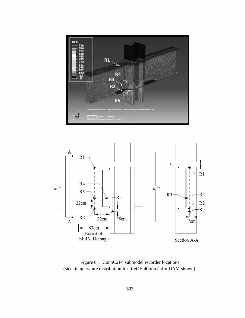
303
Figure 8.1 ConnC2F4 submodel recorder locations
(steel temperature distribution for fireOF-40min / sfrmDAM shown).

Figure 8.2 Steel temperature recordings (fireOF).
304

305
Figure 8.3 Elastic modulus of the heat-affected steel (fireOF).
Figure 8.4 Yield stress of the heat-affected steel (fireOF).

Figure 8.5 Steel temperature recordings (fireLC).
306

307
Figure 8.6 Elastic modulus of the heat-affected steel (fireLC).
Figure 8.7 Yield stress of the heat-affected steel (fireLC).

Figure 8.8 Moment-rotation response for ConnC2F4 (fireOF).
308

Figure 8.9 Moment-rotation response for ConnC2F4 (fireLC).
309

Figure 8.10 Moment-rotation response for ConnC2F4 (protected cases).
310

Figure 8.11 Moment-rotation response for ConnC2F4 (damaged cases).
311

Figure 8.12 Moment-rotation response for ConnC2F4 (effect of restrained thermal expansion).
312

313
CHAPTER 9
GLOBAL SIMULATION OF SIDESWAY RESPONSE
DURING POST-EARTHQUAKE FIRE EXPOSURE
9.1 OVERVIEW
Thermomechanical simulations of moment-frame beam-column subassemblage response
during post-earthquake fire exposure (Chapters 7 and 8) indicate that seismic damage to
spray-applied fire-resistive (SFRM) insulation in beam hinge regions leads to increased
heat penetration and temperature-induced softening of moment-rotation response for the
beam-column assembly. This chapter examines the influence of temperature-induced
moment-frame beam-column connection softening on global sidesway reponse during
post-earthquake fire exposure.
The effect of temperature-induced beam hinge softening on sidesway response of the
heat-affected stories is influenced by the residual force system in the damaged building.
In an earthquake damaged structure, these residual force demands consist of the
following components: (1) gravity forces from the tributary building mass; (2)
destabilizing forces due to the gravity loads acting through the residual post-earthquake
displacements; and (3) internal elastic restoring forces due to residual plastic
deformations in the system. If the load effects of destabilizing forces in the system are
large relative to the load effects from internal elastic restoring forces, temperature-
induced beam hinge softening (which reduces the restoring force that the beam provides
against column rotation) can lead to an increase in system drift demands during fire

314
exposure. On the other hand, if elastic restoring forces are dominant, the softened beam
hinges can provide a mechanism for internal stress reduction in the system, i.e. restoring
forces from elastically deformed beams and columns drive deformations in the softened
hinges to relieve residual stress demands in the system. The objective of the global
sidesway response analyses is therefore to evaluate the following conjectures:
Do second-order destabilizing forces in the system exacerbate drift demands during
fire exposure due to a reduction in the lateral load resistance of the heat-affected
moment-frames, and is there a possibility for progressive sidesway collapse?
Do elastic restoring forces in the system deform the softened beam hinge regions to
relieve internal stress demands due to residual plastic deformations?
The following sections present the analytical model and simulation process developed for
evaluating global sidesway response during post-earthquake fire exposure. An overview
of the analytical approach, model structure, and assumptions/limitations are presented in
Section 9.2. Section 9.3 outlines the simulation methodology developed for the multi-
hazard assessment. The test matrix for the study is presented in Section 9.4. Results
from the study are discussed in Chapter 10.
9.2 ANALYTICAL MODEL
Two large displacement analytical models were developed in the nonlinear finite element
software Abaqus (Abaqus, 2011) to study sidesway response of the test structure during
post-earthquake fire exposure: (1) a large-displacement model employing a gravity

315
loaded leaning column substructure; and (2) and a large-displacement model employing
iterative first-order analyses based on an equivalent lateral force system. The two models
differ only in terms of their treatment of the second-order loads. The following sections
provide an overview of the analytical framework and methodology for both numerical
models.
9.2.1 Large Displacement Analysis with Leaning Column Substructure
The large displacement model employing the leaning column substructure is presented in
Figures 9.1 and 9.2. The model incorporated two analytical substructures: (1) a
nonlinear special moment-frame (SMF) substructure used to model lateral load resistance
of the typical N-S SMF; and (2) a leaning column substructure used to model second-
order destabilizing loading from the tributary building mass. Kinematic constraints were
used to tie lateral translations at corresponding floor levels in the SMF and leaning
column substructures, thereby incorporating second-order destabilizing loads in the
analysis without overestimating the gravity forces acting on the SMF substructure. In
this approach, an iterative solution algorithm is utilized by the software to update second-
order forces based on the deformed geometry of the structure, i.e. equilibrium is
formulated on the displaced nodal coordinates. The progressive increase or decrease in
destabilizing load during sidesway response is therefore automated in the numerical
solution. This approach, however, can significantly add to the computational expense of
the simulation and is prone to issues with numerical convergence.

316
9.2.2 Large Displacement Analysis with Manually Updated Lateral Force Vector
In order to improve numerical convergence, the large displacement analysis can be
greatly simplified by using an iterative approach employing first-order inelastic analyses,
in which the global destabilizing force vector is manually updated for each iteration
based on the displaced geometry from the previous analysis. This approach greatly
reduces the computational expense of the numerical simulation and can significantly
improve numerical convergence within the analysis step. The convergence tolerance for
the study was set to a lateral displacement increment of 1mm, i.e. numerical convergence
was assumed to occur when the lateral displacement at each floor level was within 1mm
of the corresponding value from the previous iteration.
The destabilizing load for the simulation is modeled by converting the residual
destabilizing moments at the end of the earthquake simulation into an equivalent lateral
force system. A schematic of the model is presented in Figure 9.3, and a rendering of the
Abaqus model is shown in Figure 9.4. The procedure for developing the equivalent
lateral force system is illustrated in Equation 9-1.
∑
(Equation 9-1)
Where
is the equivalent lateral force at floor i
is the tributary gravity load at floor i

317
is the residual lateral displacement at floor i
is the height of story i
The manually updated large displacement model provided superior run times compared
to the automated large-displacement simulation, and was less susceptible to numerical
issues related to convergence. As a result, this approach was used exclusively for the
simulations presented in Chapter 10. It is noted, however, that both methods provide
identical numerical results, and that the large-displacement model may be preferable for
situations where automation is desirable.
9.2.3 Beam-Column Connection Model
Moment-rotation response data from the high-fidelity submodel analyses of Chapters 7
and 8 was used to develop a computationally efficient beam-column connection model
for studying global sidesway response during fire exposure. A schematic detail for the
idealized connection model was presented in Figure 9.3. Two flexible connector
elements were used to link the beam end nodes to the column elements. The connector
element provided rigid shear transfer between the linked nodes, but responded as a
flexible element for rotational displacements, i.e. the connector element responded as a
rotational spring. Since the connector elements in Abaqus are formulated for a finite
length (i.e. not zero-length elements), they were modeled with short spans relative to the
beam extensions, so as to not introduce additional flexural demands in the connection due
to eccentric shear transfer.

318
Since the objective of the study was to evaluate the effect of beam hinge softening on
sidesway response of test structure during post-earthquake fire exposure, and not to
evaluate the influence of thermally-induced large-displacement response in the floor
framing (e.g. thermal bowing), the beams were idealized as rigid sections. The
implications of this idealization are discussed in Section 9.3.3. The elastic flexibility for
each beam extension, which was not simulated by the rigid elements, was incorporated in
the calibrated moment-rotation response for the associated connector element.
Flexible columns were utilized in the connection model to account for variations in
interstory drift demand, and to model temperature-dependent mechanical response in the
fire compartment. Nonlinear, distributed plasticity, cubic-formulation, beam-column
elements (type B33 in the Abaqus element library) were selected for consistency with the
high-fidelity submodel analyses of Chapter 9.
The moment-rotation response of each connector element was calibrated by extracting
component flexibility, and then adjusting the connector models to match the target
rotational response of the beam-column subassemblage. The calibration procedure is
outlined below.
Step 1: Initially, the monotonic moment-rotation response of the connector element
is calibrated to an associated submodel analysis that employs either the nonlinear
fiber element beam-column connection model presented in Chapter 4 (for connections
at normal ambient temperature), or the high-fidelity continuum element beam-column

319
connection model presented in Chapter 7 (for connections located within the fire
compartment). For all cases, moment-rotation response is idealized with a best-fit bi-
linear backbone curve and a kinematic hardening model. Equation 9-2 presents the
relationship for the initialization step.
(Equation 9-2)
Where
is the elastic rotational stiffness of the typical connector element.
is the target equivalent elastic rotational stiffness of the beam-column
subassemblage.
Step 2: A monotonic displacement-controlled analysis is then performed to
determine the actual equivalent elastic rotational stiffness ( ) for the
initialized beam-column subassemblage from Step 1. It is noted that the initialized
model considers flexible column elements, rigid beam elements, and the initialized
flexible connector elements from Step 1.
Step 3: At this point, the typical elastic rotational stiffness of the connector elements
( ) is known from Step 1, the equivalent elastic rotational stiffness of the
initialized beam-column subassemblage ( ) is known from Step 2, and
the elastic rotational stiffness contribution from the flexible column ( ) is
unknown. The problem is analogous to a mechanical system with two springs
positioned in series, where one spring models the stiffness contribution from the

320
beams and panel zone ( ) and the second spring models the stiffness
contribution from the column ( ). Equation 9-3 can then be solved for the
stiffness contribution from the flexible column.
⁄ ( )
⁄ ⁄
(Equation 9-3)
Step 4: Once the stiffness contribution from the flexible column ( ) is known
(from Step 3), the elastic rotational stiffness of the connector elements can be
adjusted ( ) to produce an equivalent elastic rotational stiffness
( ) equal to the target response for the beam-column subassemblage
( ). The procedure is illustrated in Equation 9-4.
⁄ ⁄ ( )⁄
⁄
(Equation 9-4)
Figures 9.5-9.19 present the monontonic and cyclic moment-rotation response curves for
the calibrated beam-column connection models. The notation provided in the figures is
as follows:
connUNMOD/bmRIGID/colRIGID: Beam-column subassemblage model with rigid
beams and columns, and flexible connector elements utilizing the initialized
rotational stiffness from Step 1 ( ).

321
connUNMOD/bmRIGID/colFLEX: Beam-column subassemblage model with rigid
beams, flexible columns, and flexible connector elements utilizing the initialized
rotational stiffness from Step 1 ( ). The actual equivalent elastic rotational
stiffness ( ) of this model is determined in Step 2.
connMOD/bmRIGID/colFLEX: Beam-column subassemblage model with rigid
beams, flexible columns, and flexible connector elements utilizing the adjusted
rotational stiffness from Step 4 ( ). The actual equivalent elastic rotational
stiffness ( ) is calibrated to match the target rotational stiffness for the
beam-column subassemblage.
For the cyclic response analyses, a displacement-controlled approach was implemented
using the linearized ConnC2F4-EQ11A deformation history presented in Figure 7.38. In
general, very good agreement was found between the cyclic response predictions from
the beam-column connection model developed in this chapter and the beam-column
models developed in either Chapter 4 (for connections at normal ambient temperature) or
Chapter 7 (for connections located within the fire compartment).
The objective of this task was to develop a computationally efficient beam-column
connection model that: (1) could replicate the cyclic inelastic behavior of the dynamic
response model beam-column connections in order develop the post-earthquake damaged
building, capturing the residual force and deformation demands in the system; and (2)
could provide a simple means for incorporating the complex fire-related effects observed
in the high-fidelity submodel simulations of Chapter 7.

322
9.2.4 Column Base Regions
The column base regions were modeled with 20-node, quadratic, fully-integrated
continuum stress analysis elements (type C3D20 in the Abaqus element library) in order
to account for inelastic hinging. Mulit-point kinematic constraints were used to enforce
compatibility at the continuum element-to-linear element transitions, as shown in Figure
9.20. This approach used a kinematic constraint law to slave the nodal translations on the
connecting surface of the continuum body to the nodal displacements of the connecting
beam node (designated as the control node). The constraint considered eccentricity
between the control node and the slaved nodes and was therefore capable of transferring
translational and rotational displacements between the joined parts.
9.2.5 Gravity Loads
Gravity loads for the test structure were presented in Section 3.4. Member loads were
applied to the SMF substructure to model tributary gravity loading on the lateral force
resisting elements. Concentrated loads were applied to the leaning column substructure
to model the gravity load demands for the half-system submodel (excluding gravity loads
applied directly to the SMF substructure). It is noted that the load factors were adjusted
in accordance with FEMA P695 (FEMA, 2008) to represent expected (or probable)
loading conditions, using the load case presented in Equation 4-20.

323
9.3 SIMULATION METHODOLOGY AND EXECUTION
9.3.1 Overview
A multi-step sequential analysis approach was developed to simulate seismic response of
the test structure to MCE ground shaking and thermal degradation during post-earthquake
fire exposure. The initial earthquake simulation utilized a pseudo-dynamic approach,
employing a series of sequential static analysis steps, to impose lateral floor displacement
histories from the nonlinear response history analyses of Chapter 6. The procedure is
shown schematically in Figure 9.21. The objective of this analysis step was to develop
the residual force and deformation demands in the damaged building. A post-earthquake
fire simulation was then performed, within the same model space, as a series of static
analysis steps by adjusting the mechanical properties of the heat-affected elements to
account for thermal degradation. The procedure is shown schematically in Figure 9.22.
It is noted that each analysis step for the post-earthquake fire simulation was
representative of a discrete time instance during the simulation.
9.3.2 Step 1 - Earthquake Simulation
A pseudo-dynamic approach was utilized to simulate seismic response of the test
structure for two MCE events by imposing the lateral floor displacement histories from
Chapter 6. The objective of this analysis step was to develop the residual force and
deformation demands in the damaged building. Records EQ11A (Landers, CA, 1992)
and EQ17A (Superstition Hills, CA, 1987) were selected based on the following
considerations: (1) both records produced peak interstory drift demands (an indicator of
connection rotational demand) larger than 3%, indicating a high probability for SFRM

324
damage based on the fragility function developed in Section 7.2.6; (2) both records
produced large destabilizing moment at the fourth elevated floor relative to the MCE
record ensemble (note: simulated fire compartments located on the 2nd
, 3rd
, and 4th
floors); (3) both records were from southern California events and were therefore
consistent with the site conditions assumed in the design process; and (4) both records
were from relatively recent events and were obtained using modern recording devices.
Dynamic response analyses for the records were presented in Chapter 6. A summary of
relevant response parameters is provided in Table 9-1.
Time-history deformation demands for each record were simulated by imposing nodal
displacement histories from the dynamic simulations of Chapter 6. A rendering of the
Abaqus model for the earthquake simulation step is presented in Figure 9.23. The
earthquake response records were idealized by considering discrete time points related to
local peaks in rotational demand in ConnC2F4, i.e. the lateral displacement histories at
the floor levels were specified at time points corresponding to local peaks in rotational
demand for ConnC2F4. This approach was considered as a reasonable discretization
since the dynamic response for both records was dominated by the fundamental mode of
vibration, as shown in Figures 6.57 and 6.63. The deformed geometry in the Abaqus
model at peak drift demand for the EQ11A record is shown in Figure 9.23.
Figures 9.24 and 9.25 present the selected time points for the EQ11A and EQ17A
simulations, respectively. The idealized floor displacement histories, superimposed on

325
the recorded floor displacement histories, are presented in Figures 9.26-9.35 for EQ11A
and Figures 9.36-9.45 for EQ17A.
9.3.3 Step 2 - Post-Earthquake Fire Simulation
The post-earthquake fire simulation was performed by adjusting the mechanical
properties of the connector and column elements for temperature effects. The procedure
was shown schematically in Figure 9.22. The column sections were updated during the
simulation through the load module by directly specifying steel temperatures at the
section integration points, discussed further in Section 9.4. The connector sections were
updated in a similar manner using the idealized temperature-dependent moment-rotation
curves developed in Section 9.2.3. At the selected time instances during the fire
simulation, static analyses were performed to determine the transient state of equilibrium
in the structure.
9.3.4 Assumptions and Limitations
As previously discussed, the objective of this study was to evaluate the effect of
temperature-induced beam hinge softening on global sidesway response during post-
earthquake fire exposure. The numerical simulation presented in the preceding sections
therefore provides an idealized model for system behavior during fire exposure that only
captures the response mode and parameters of interest. The following limitations in the
analysis are noted:

326
The simulation considers uncoupled unidirectional response and therefore neglects
the effect of out-of-plane deformations and force demands on in-plane behavior.
The simulation neglects forces transferred to the columns due to restrained thermal
expansion and large displacement response of the floor system, as illustrated in
Figure 9.46. It is noted, however, that the effect of restrained thermal expansion on
beam hinge softening was included in the submodel analyses of Chapters 7 and 8,
which were utilized to calibrate the nonlinear connector elements discussed in Section
9.2.3.
The simulation neglects the effect of restrained thermal expansion in the columns.
This effect was thought to have less of an influence on sidesway response than beam
hinge softening since steel temperatures in the column remain relatively low.
The simulation neglects the lateral resistance provided by the gravity frames, infill
walls, and external cladding. This assumption was considered as a reasonable
simplification since the lateral resistance is predominately provided by the perimeter
moment-frames.
9.3.5 Execution
The Abaqus job files were executed on Lehigh University’s high performance Linux
Beowulf cluster Blaze, which contains a total of 120 64-bit AMD Opteron processors and
2G of RAM per node, with an approximate run time of 60-minutes for the Phase 1 –
earthquake simulations and 15-minutes for the Phase 2 – post-earthquake fire
simulations.

327
9.4 TEST MATRIX
The test matrix for the global sidesway simulation study is presented in Tables 9-2
through 9-4. The test program included six conceptual post-earthquake fire scenarios
(Section 9.4.1), used to evaluate behavioral response and to assess the efficacy of existing
building code requirements for the multi-hazard scenario, and a supporting parametric
study to identify potential vulnerabilities related to temperature-induced beam hinge
softening (Section 9.4.3) and column softening (Section 9.4.4).
The post-earthquake fire simulations assumed fully developed fires applied instanteously
and uniformly over the building floor plan, and utilized the time-temperature data from
the large compartment fire simulation (fireLC) discussed in Section 7.2.5. The large
compartment fire simulation was considered as a more representative model for a fully
developed floor fire than the hotter and shorter duration office fire simulation (fireOF) of
Section 7.2.5.
9.4.1 Post-Earthquake Fire Scenarios
Six conceptual post-earthquake fire scenarios were evaluated utilizing two earthquake
response records (EQ11A and EQ17A) and three fire scenarios (fireLCF3, fireLCF23,
and fireLCF234). The fire scenarios utilized in the simulations are described below.
fireLCF3 (single-floor fire simulation) – fire scenario utilizing the fireLC temperature
history applied uniformly and instantaneously over the third elevated floor.

328
fireLCF23 (two-floor fire simulation) – fire scenario utilizing the fireLC temperature
history applied uniformly and instantaneously over the second and third elevated
floors.
fireLCF234 (three-floor fire simulation) – fire scenario utilizing the fireLC
temperature history applied uniformly and instantaneously over the second, third, and
fourth elevated floors.
The post-earthquake fire scenarios utilized the large displacement analysis procedure
discussed in Section 9.2.2. Based on the seismic fragility model for SFRM insulation
developed in Section 7.2.6, all connector elements located within the designated fire
compartment were assumed to follow the calibrated temperature-dependent moment-
rotation response model developed in Section 9.2.3 (designated as bhFLEX). Steel
temperatures in the column sections located within the fire compartment were based on
the recorded temperature distributions from the Chapter 8 heat transfer simulations
(designated as colREC), considering a prismatic section located away from the beam-
column joint. Figure 9.47 presents the typical steel temperature distribution utilized for
the column sections at 20min, 40min, and 60min into the large compartment fire
simulation. The post-earthquake fire scenarios are identified in Table 9.2 as follows:
Scenario 1: EQ11A / fireLCF3 / bhFLEX / colREC
Scenario 2: EQ11A / fireLCF23 / bhFLEX / colREC
Scenario 3: EQ11A / fireLCF234 / bhFLEX / colREC
Scenario 4: EQ17A / fireLCF3 / bhFLEX / colREC

329
Scenario 5: EQ17A / fireLCF23 / bhFLEX / colREC
Scenario 6: EQ17A / fireLCF234 / bhFLEX / colREC
9.4.2 Influence of Temperature-Induced Beam Hinge Softening
Six test models were developed to evaluate the limiting case where the heat-affected
beams in the fire compartment no longer restrain the rotations of the respective columns,
i.e. pinned beam-column connections. The test cases developed for this study utilized the
pseudo-large displacement analysis discussed in Section 9.2.2. Both the EQ11A and
EQ17A seismic response records were investigated. Steel temperatures for the columns
within the fire compartment were based on the colREC temperature profiles. Single-floor
and multi-floor fire scenarios were investigated. The test cases are identified in Table 9-3
as follows:
Scenario 7: EQ11A / fireLCF3 / bhPIN / colREC
Scenario 8: EQ11A / fireLCF23 / bhPIN / colREC
Scenario 9: EQ11A / fireLCF234 / bhPIN / colREC
Scenario 10: EQ17A / fireLCF3 / bhPIN / colREC
Scenario 11: EQ17A / fireLCF23 / bhPIN / colREC
Scenario 12: EQ17A / fireLCF234 / bhPIN / colREC
9.4.3 Influence of Temperature-Induced Column Softening
Strong column-weak beam response is ensured in well-designed ductile steel moment-
frames through prescriptive strength and detailing requirements. In these systems,

330
inelastic deformations are concentrated in the beam hinge regions, while stress demands
in the column sections remain within the elastic range (as was shown in Chapter 6). As a
result, anticipated SFRM damage during seismic response is limited to the beam hinge
regions, while moment-frame column sections are assumed to be fully insulated in the
event of a post-earthquake fire.
Buildings constructed prior to the adoption of the modern strong column-weak beam
design guidelines, however, may be subject to inelastic deformations in the moment-
frame columns, which could potentially damage SFRM insulation and expose regions of
unprotected steel to elevated ambient temperatures during a post-earthquake fire. In
order to evaluate the influence of temperature-induced column softening on sidesway
response, the columns within the designated fire compartment were heated to 300oC,
400oC, and 500
oC (designated as colTEMP), which correspond to elastic modulus
reductions of 20%, 30%, and 40%, respectively (or kE,T of 80%, 70%, and 60%). The test
cases developed for this study utilized the pseudo-large displacement analysis discussed
in Section 9.2.2. Both the EQ11A and EQ17A seismic response record were
investigated. The bhFLEX connector model was assumed for all cases, and both single-
floor and multi-floor fire scenarios were evaluated. The test cases are identified in Table
9-4 as follows:
Case 13: EQ11A / fireLCF3 / bhFLEX / col300
Case 14: EQ11A / fireLCF3 / bhFLEX / col400
Case 15: EQ11A / fireLCF3 / bhFLEX / col500

331
Case 16: EQ11A / fireLCF23 / bhFLEX / col300
Case 17: EQ11A / fireLCF23 / bhFLEX / col400
Case 18: EQ11A / fireLCF23 / bhFLEX / col500
Case 19: EQ17A / fireLCF3 / bhFLEX / col300
Case 20: EQ17A / fireLCF3 / bhFLEX / col400
Case 21: EQ17A / fireLCF3 / bhFLEX / col500
Case 22: EQ17A / fireLCF23 / bhFLEX / col300
Case 23: EQ17A / fireLCF23 / bhFLEX / col400
Case 24: EQ17A / fireLCF23 / bhFLEX / col500
9.5 SUMMARY
A nonlinear numerical model and multi-step simulation process for evaluating global
sidesway response during post-earthquake fire exposure was developed in this chapter.
Computationally efficient beam-column connection models were developed using
response data from the high-fidelity thermomechanical submodel simulations of
Chapter 8. The simulation utilized a pseudo-dynamic displacement-controlled procedure,
based on response data from the nonlinear dynamic analyses of Chapter 6, to simulate
seismic response of the test structure, with the objective of developing the post-
earthquake damaged condition. A series of post-earthquake fire simulations were then
performed by adjusting the mechanical response of structural elements located within the
fire compartment to account for temperature effects. At selected time instances during
the fire simulation, large displacement static analyses were utilized to determine to the
transient state of equilibrium for the system. The test matrix for the study included six

332
conceptual post-earthquake fire scenarios, which were utilized to evaluate behavioral
response and to assess the efficacy of existing building code requirements for the multi-
hazard scenario, and a supporting parametric study to identify potential vulnerabilities
related to temperature-induced beam hinge and column softening.

Table 9.1 Earthquake response records
SMT /SMT Peak Residual Peak Residual Peak Residual (kN-m)
11ALANDERS/
YER270
Landers, CA
(1992)1.13 3.17% 1.59% 3.38% 1.82% 3.47% 1.90%
1.57E4
(91st
percentile)
17ASUPERST/
B-POE270
Superstition
Hills, CA
(1987)
1.55 3.91% 2.02% 3.68% 2.13% 3.33% 2.10%1.22E4
(86th
percentile)
Story 5Story 4
Interstory Drift Demand (%) Residual
Destabilizing
Moment about
the 4th FloorSpectral
DemandStory 3Record
ID
PEER
File Name
Location
(Date)
333

Table 9.2 Test matrix - post-earthquake fire simulations
EQ11A EQ17ASingle-Floor
F3
Two-Floor
F2, F3
Three-Floor
F2, F3, F4
Flexible
Connector
M (θ,T)
Pin
Connector
M = 0
fireLC
Record
300oC
(kE,T = 0.80)
400oC
(kE,T = 0.70)
500oC
(kE,T = 0.60)
1EQ11A / fireLCF3 /
bhFLEX / colREC
2EQ11A / fireLCF23 /
bhFLEX / colREC
3EQ11A / fireLCF234 /
bhFLEX / colREC
4EQ17A / fireLCF3 /
bhFLEX / colREC
5EQ17A / fireLCF23 /
bhFLEX / colREC
6EQ17A / fireLCF234 /
bhFLEX / colREC
Column Softening
Scenario
No.ID
Earthquake Response
RecordFire Scenario (fireLC) Beam Hinge Softening
334

Table 9.3 Test matrix - influence of temperature-induced beam hinge softening
EQ11A EQ17ASingle-Floor
F3
Two-Floor
F2, F3
Three-Floor
F2, F3, F4
Flexible
Connector
M (θ,T)
Pin
Connector
M = 0
fireLC
Record
300oC
(kE,T = 0.80)
400oC
(kE,T = 0.70)
500oC
(kE,T = 0.60)
7EQ11A / fireLCF3 /
bhPIN / colREC
8EQ11A / fireLCF23 /
bhPIN / colREC
9EQ11A / fireLCF234 /
bhPIN / colREC
10EQ17A / fireLCF3 /
bhPIN / colREC
11EQ17A / fireLCF23 /
bhPIN / colREC
12EQ17A / fireLCF234 /
bhPIN / colREC
Column Softening
Scenario
No.ID
Earthquake Response
RecordFire Scenario (fireLC) Beam Hinge Softening
335
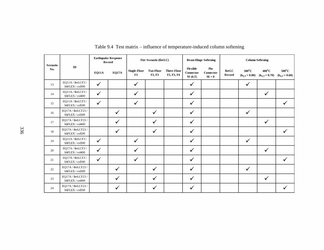
Table 9.4 Test matrix – influence of temperature-induced column softening
EQ11A EQ17ASingle-Floor
F3
Two-Floor
F2, F3
Three-Floor
F2, F3, F4
Flexible
Connector
M (θ,T)
Pin
Connector
M = 0
fireLC
Record
300oC
(kE,T = 0.80)
400oC
(kE,T = 0.70)
500oC
(kE,T = 0.60)
13EQ11A / fireLCF3 /
bhFLEX / col300
14EQ11A / fireLCF3 /
bhFLEX / col400
15EQ11A / fireLCF3 /
bhFLEX / col500
16EQ17A / fireLCF23 /
bhFLEX / col300
17EQ17A / fireLCF23 /
bhFLEX / col400
18EQ17A / fireLCF23 /
bhFLEX / col500
19EQ11A / fireLCF3 /
bhFLEX / col300
20EQ17A / fireLCF3 /
bhFLEX / col400
21EQ17A / fireLCF3 /
bhFLEX / col500
22EQ17A / fireLCF23 /
bhFLEX / col300
23EQ17A / fireLCF23 /
bhFLEX / col400
24EQ17A / fireLCF23 /
bhFLEX / col500
Column Softening
Scenario
No.ID
Earthquake Response
RecordFire Scenario (fireLC) Beam Hinge Softening
336

337
Figure 9.1 Large displacement model with leaning column substructure.
Figure 9.2 Large displacement Abaqus model with leaning column substructure.
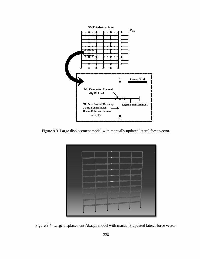
338
Figure 9.3 Large displacement model with manually updated lateral force vector.
Figure 9.4 Large displacement Abaqus model with manually updated lateral force vector.

339
Figure 9.5 Monotonic moment-rotation response,
1st and 2
nd floor beam-column connections at normal ambient temperature.
Figure 9.6 Cyclic moment-rotation response for the ConnC2F4-EQ11A record,
1st and 2
nd floor beam-column connections at normal ambient temperature.

340
Figure 9.7 Monotonic moment-rotation response,
3rd
and 4th
floor beam-column connections at normal ambient temperature.
Figure 9.8 Cyclic moment-rotation response for the ConnC2F4-EQ11A record,
3rd
and 4th
floor beam-column connections at normal ambient temperature.

341
Figure 9.9 Monotonic moment-rotation response,
5th
and 6th
floor beam-column connections at normal ambient temperature.
Figure 9.10 Cyclic moment-rotation response for the ConnC2F4-EQ11A record,
5th
and 6th
floor beam-column connections at normal ambient temperature.

342
Figure 9.11 Monotonic moment-rotation response,
7th
and 8th
floor beam-column connections at normal ambient temperature.
Figure 9.12 Cyclic moment-rotation response for the ConnC2F4-EQ11A record,
7th
and 8th
floor beam-column connections at normal ambient temperature.

343
Figure 9.13 Monotonic moment-rotation response,
9th
floor beam-column connections at normal ambient temperature.
Figure 9.14 Cyclic moment-rotation response for the ConnC2F4-EQ11A record,
9th
floor beam-column connections at normal ambient temperature.

344
Figure 9.15 Monotonic moment-rotation response,
10th
floor beam-column connections at normal ambient temperature.
Figure 9.16 Cyclic moment-rotation response for the ConnC2F4-EQ11A record,
10th
floor beam-column connections at normal ambient temperature.

345
Figure 9.17 Monotonic moment-rotation response,
3rd
and 4th
floor beam-column connections at 20min (fireLC).
Figure 9.18 Monotonic moment-rotation response,
3rd
and 4th
floor beam-column connections at 40min (fireLC).

346
Figure 9.19 Monotonic moment-rotation response,
3rd
and 4th
floor beam-column connections at 60min (fireLC).
Figure 9.20 Column base region: multi-point kinematic constraint
at the continuum element-to-linear element transition.

347
Figure 9.21 Step 1 – Earthquake simulation.
Figure 9.22 Step 2 – Post-earthquake fire simulation.

348
(a)
(b)
Figure 9.23 Step 1 – earthquake simulation Abaqus model: (a) boundary conditions;
(b) deformed geometry at peak drift demand for EQ11A (scale: x5).

349
Figure 9.24 Selected time points for EQ11A simulation.
Figure 9.25 Selected time points for EQ17A simulation.

350
Figure 9.26 Lateral displacement history at the 1st elevated floor (EQ11A).
Figure 9.27 Lateral displacement history at the 2nd
elevated floor (EQ11A).

351
Figure 9.28 Lateral displacement history at the 3rd
elevated floor (EQ11A).
Figure 9.29 Lateral displacement history at the 4th
elevated floor (EQ11A).

352
Figure 9.30 Lateral displacement history at the 5th
elevated floor (EQ11A).
Figure 9.31 Lateral displacement history at the 6th
elevated floor (EQ11A).

353
Figure 9.32 Lateral displacement history at the 7th
elevated floor (EQ11A).
Figure 9.33 Lateral displacement history at the 8th
elevated floor (EQ11A).

354
Figure 9.34 Lateral displacement history at the 9th
elevated floor (EQ11A).
Figure 9.35 Lateral displacement history at the roof (EQ11A).

355
Figure 9.36 Lateral displacement history at the 1st elevated floor (EQ17A).
Figure 9.37 Lateral displacement history at the 2nd
elevated floor (EQ17A).

356
Figure 9.38 Lateral displacement history at the 3rd
elevated floor (EQ17A).
Figure 9.39 Lateral displacement history at the 4th
elevated floor (EQ17A).

357
Figure 9.40 Lateral displacement history at the 5th
elevated floor (EQ17A).
Figure 9.41 Lateral displacement history at the 6th
elevated floor (EQ17A).
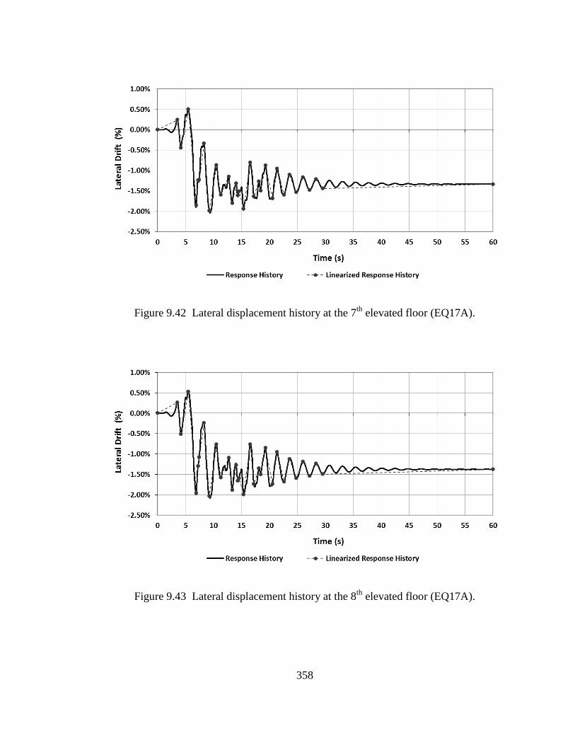
358
Figure 9.42 Lateral displacement history at the 7th
elevated floor (EQ17A).
Figure 9.43 Lateral displacement history at the 8th
elevated floor (EQ17A).

359
Figure 9.44 Lateral displacement history at the 9th
elevated floor (EQ17A).
Figure 9.45 Lateral displacement history at the roof (EQ17A).

360
Figure 9.46 Forces developed due to restrained thermal expansion
and temperature-induced large displacement response in the floor system.
(a) (b) (c)
Figure 9.47 Steel temperatures at the column integration points:
(a) fireLC-20min; (b) fireLC-40min; (c) fireLC-60min.

361
CHAPTER 10
GLOBAL SIMULATION OF SIDESWAY RESPONSE
DURING POST-EARTHQUAKE FIRE EXPOSURE
- ANALYTICAL RESULTS
10.1 OVERVIEW
This chapter presents results from numerical simulations of global sidesway response
during post-earthquake fire exposure. The analytical model and simulation process were
discussed in Chapter 9. Section 10.2 presents results from six conceptual post-earthquake
fire scenarios, used to evaluate the effect of temperature-induced moment-frame beam
hinge softening on sidesway response in the heat-affected stories, and to assess the
efficacy of existing building code provisions for the multi-hazard post-earthquake fire
scenario. Sections 10.3 and 10.4 present results from a parametric study designed to
identify potential vulnerabilities associated with temperature-induced beam hinge and
temperature-induced column softening, respectively.
10.2 POST-EARTHQUAKE FIRE SCENARIOS
This section presents results from six post-earthquake fire scenarios. The study considers
two seismic response records (EQ11A and EQ17A) from Chapter 6, and three fire
exposure conditions (fireLCF2, fireLCF23, and fireLCF234), defined in Chapter 9.
10.2.1 Scenario 1: EQ11A – Single-Floor Fire Simulation
Drift demands, lateral floor displacements, and interstory drift ratios are presented in
Figures 10.1-10.3, respectively, at 20min, 40min, and 60min into the single-floor, post-

362
EQ11A fire simulation. The corresponding rotational demand in ConnC2F4 (refer to
Figure 4.1) is shown in Figure 10.4. A summary of the response data is provided in
Tables 10.1-10.3.
Figures 10.1 and 10.3 demonstrate that the test structure remains stable during the single-
floor fire simulation with only small fluctuations in lateral floor displacement relative to
the residual post-earthquake drift demands. Although the temperature-induced
displacements are negligible for practical considerations, they do provide insight into the
behavior of the test structure during fire exposure. Figures 10.2 and 10.4 illustrate that
heat induced softening of the beam hinge and column regions within the fire
compartment leads to a progressive increase in interstory drift demand in the 3rd
through
5th
stories, and rotational demand in the associated beam-column connections. The
largest change in interstory drift occurs at 60min into the fire simulation in the 3rd
story,
where the interstory drift demand increases from 1.60% to 1.61% (+ 0.01%).
Figure 10.2 also shows a progressive increase in lateral displacement at the 2nd
, 3rd
, and
4th
elevated floors, which indicates that second-order destabilizing forces drive
deformation demands in the softened beam hinge regions. Above the 4th
elevated floor,
the lateral displacements are smaller than the values at floors 3 and 4, which indicates
that the upper region of the building is rotating in a “centering” motion, and is likely
influenced by elastic restoring forces.

363
10.2.2 Scenario 2: EQ11A – Two-Floor Fire Simulation
Drift demands, lateral floor displacements, and interstory drift ratios are presented in
Figures 10.5-10.7, respectively, at 20min, 40min, and 60min into the two-floor, post-
EQ11A fire simulation. The corresponding rotational demand in ConnC2F4 is shown in
Figure 10.8. A summary of the response data is provided in Tables 10.1-10.3.
The test structure remains stable during the two-floor fire simulation with only small
increases in lateral floor displacement relative to the residual post-earthquake drift
demands, as illustrated in Figures 10.5 and 10.7. In a similar manner to the single-floor
fire simulation in Scenario 1, temperature-induced softening of the beam hinge and
column regions within the fire compartment leads to a progressive increase in interstory
drift demand in the 3rd
and 4th
stories (Figure 10.6), and rotational demand in the
associated beam-column connections (Figure 10.8). The largest change in interstory drift
occurs at 60min into the fire simulation in the 3rd
story, where the interstory drift demand
increases from 1.60% to 1.63% (+ 0.03%).
The two-floor fire simulation exhibits similar behavioral characteristics to the single-floor
fire simulation of Scenario 1. Figure 10.6 shows a progressive increase in lateral
displacement at the 1st through 4
th elevated floors, which indicates the relative influence
of second-order destabilizing forces in this region. The lateral displacements in the upper
region of the building are smaller than the values at floor 4, which indicates a “centering”
motion that is likely influenced by elastic restoring forces.

364
10.2.3 Scenario 3: EQ11A – Three-Floor Fire Simulation
Drift demands, lateral floor displacements, and interstory drift ratios are presented in
Figures 10.9-10.11, respectively, at 20min, 40min, and 60min into the three-floor, post-
EQ11A fire simulation. The corresponding rotational demand in ConnC2F4 is shown in
Figure 10.12. A summary of the response data is provided in Tables 10.1-10.3.
During the three-floor fire simulation, temperature-induced beam hinge and column
softening exacerbates interstory drift demands in the 3rd
through 6th
stories (as illustrated
in Figures 10.9 and 10.11), although the increases are still small relative to the residual
post-earthquake drift demands. The largest changes in interstory drift occur at 60min into
the fire simulation in the 4th
through 6th
stories, where the interstory drift demand
increases by +0.04-0.05%. As shown in Figure 10.10, the lateral floor displacements
progressively increase over the building height, which indicates the dominance of
destabilizing forces.
10.2.4 Scenario 4: EQ17A – Single-Floor Fire Simulation
Drift demands, lateral floor displacements, and interstory drift ratios are presented in
Figures 10.13-10.15, respectively, at 20min, 40min, and 60min into the single-floor, post-
EQ17A fire simulation. The corresponding rotational demand in ConnC2F4 is shown in
Figure 10.16. A summary of the response data is provided in Tables 10.1-10.3.
Figures 10.13 and 10.15 demonstrate that the test structure remains stable during the
single-floor fire simulation with only small increases in lateral floor displacement relative

365
to the residual post-earthquake drift demands. Figures 10.14 and 10.16 illustrate that heat
induced softening of the beam hinge and column regions within the fire compartment
leads to a progressive increase in interstory drift demand in the 3rd
through 5th
elevated
floors, and rotational demand in the associated beam-column connections, although the
increase is negligible for practical considerations. The largest change in interstory drift
occurs at 60min into the fire simulation in the 4th
story, where the interstory drift demand
increases from 2.18% to 2.21% (+ 0.03%). As shown in Figure 10.15, the lateral floor
displacements progressively increase over the building height, which indicates the
dominance of destabilizing forces in the heat-affected region. It is noted that the
progressive increase in floor displacement in the upper region of the building is most
likely influenced by elastic restoring forces.
10.2.5 Scenario 5: EQ17A – Two-Floor Fire Simulation
Drift demands, lateral floor displacements, and interstory drift ratios are presented in
Figures 10.17-10.19, respectively, at 20min, 40min, and 60min into the two-floor, post-
EQ17A fire simulation. The corresponding rotational demand in ConnC2F4 is shown in
Figure 10.20. A summary of the response data is provided in Tables 10.1-10.3.
The test structure remains stable during the two-floor fire simulation with only small
increases in lateral floor displacement relative to the residual post-earthquake drift
demands, as illustrated in Figures 10.17 and 10.9. Although negligible for practical
considerations, Figures 10.18 and 10.20 illustrate that heat induced softening of the beam
hinge and column regions within the fire compartment leads to a progressive increase in

366
interstory drift demand in the 3rd
through 5th
stories, and rotational demand in the
associated beam-column connections. The largest change in interstory drift occurs at
60min into the fire simulation in the 4th
story, where the interstory drift demand increases
from 2.18% to 2.23% (+0.05%). The two-floor fire simulation exhibits similar
behavioral characteristics to the single-floor fire simulation of Scenario 5. The
progressive increase in lateral floor displacement over the building height is indicative of
destabilizing force demands in the heat-affected region and elastic restoring forces in the
upper region of the building.
10.2.6 Scenario 6: EQ17A – Three-Floor Fire Simulation
Drift demands, lateral floor displacements, and interstory drift ratios are presented in
Figures 10.21-10.23, respectively, at 20min, 40min, and 60min into the three-floor, post-
EQ17A fire simulation. The corresponding rotational demand in ConnC2F4 is shown in
Figure 10.24. A summary of the response data is provided in Tables 10.1-10.3.
During the three-floor fire simulation, temperature-induced beam hinge and column
softening exacerbates interstory drift demands in the 3rd
through 5th
stories, as illustrated
in Figures 10.22. The largest change in interstory drift occurs at 60min into the fire
simulation in the 4th
story, where the interstory drift demand propagates from 2.18% to
2.23% (+0.05%).
Figure 10.22 also illustrates that the lateral floor displacements at floors 1 through 5
increase progressively with height, indicating the dominance of destabilizing forces in the

367
heat-affected region. Above the 5th
floor, the lateral displacements are slightly lower than
the value at floor 5, which indicates that destabilizing forces are likely driving the
deformation response in the upper region of the building.
10.2.7 Discussion
The test structure remained stable during the single-floor and multi-floor post-earthquake
fire simulations with only small fluctuations in floor displacement. An explanation for
this behavior is as follows: Existing building code provisions incorporate stringent drift
control and ductility requirements to improve seismic performance. These requirements
generally necessitate the use of deep beams and heavy column sections in moment-frame
designs. The large volume-to-surface area ratio of these heavy column sections enhances
their resistance to ambient heating and makes them less susceptible to fire effects,
especially considering that the thermal insulation for the columns is not damaged during
seismic response. As a result, the moment-frame columns provide considerable restraint
against sidesway deformations in the system during fire exposure, even with substantial
temperature-induced softening of the beam hinge regions along multiple floor levels.
The considerable rotational stiffness retained in the heat-affected beam hinge regions, due
to limited heat penetration near the SFRM damage sites (as shown in Chapter 8), also
provides a major contribution to the inherent resistance of moment-frame buildings to
sidesway deformations during post-earthquake fire exposure.
The conceptual post-earthquake fire analyses of Sections 10.2.1-10.26 do provide insight
regarding the behavioral response and driving forces during post-earthquake fire

368
exposure. Deformation response in the heat-affected stories and lower regions of the
building was generally influenced by destabilizing force demands, as evidenced by a
progressive increase in interstory drift demands, oriented in the destabilizing direction.
The upper region of the building tended to exhibit a “centering” response, likely driven
by elastic restoring forces and facilitated by the softened beam-column connections in the
heat-affected region. As expected, softening of beam-column connections along multiple
floor levels increased susceptibility to sidesway deformation, leading to moderate
increases in interstory drift demand.
10.3 INFLUENCE OF TEMPERATURE-INDUCED BEAM HINGE SOFTENING
It is speculated that thinner beam sections may be more susceptible to heat penetration
and thermal degradation of moment-rotation response than the W840x193 beam section
evaluated in the ConnC2F4 subassemblage. The relative area of exposed steel (extent of
SFRM damage) in the beam hinge region will also have a significant effect on the heat
flux boundary surface, and could significantly increase temperature propagation and
thermal degradation in the beam hinge region. As a result, the following section presents
results from six test models developed to evaluate the limiting case where the heat-
affected beams in the fire compartment no longer restrain the rotations of the respective
columns, i.e. pinned beam-column connections. The study considers two seismic
response records (EQ11A and EQ17A) from Chapter 6, and three fire exposure
conditions (fireLCF2, fireLCF23, and fireLCF234), discussed in Chapter 9.

369
10.3.1 Scenario 7: EQ11A – Single-Floor Fire Simulation
Drift demands, lateral floor displacements, and interstory drift ratios are presented in
Figures 10.25-10.27 at 60min into the single-floor, post-EQ11A fire simulation,
considering loss of rotational restraint at the beam-column connections along the 4th
elevated floor. The corresponding rotational demand in ConnC2F4 is shown in Figure
10.28. For comparison purposes, the response parameters are plotted with the
corresponding values from Scenario 1, which uses the bhFLEX connector model. A
summary of the response data is provided in Tables 10.4.
Figures 10.25 and 10.27 demonstrate that the test structure remains stable during the
single-floor fire simulation with only small fluctuations in floor displacement relative to
the residual post-earthquake drifts. Total loss of rotational continuity at the beam-column
connections within the fire compartment leads to a “centering” response in the test
structure that is driven by elastic restoring forces. This is in contrast to Scenario 1, where
destabilizing forces dominate response in the heat-affected region. The largest reductions
in interstory drift demand are observed in the 4th
and 5th
stories, where the interstory drift
demand decreases from 1.88% to 1.84% (-0.04%) and 1.91% to 1.86% (-0.05%),
respectively.
10.3.2 Scenario 8: EQ11A – Two-Floor Fire Simulation
Drift demands, lateral floor displacements, and interstory drift ratios are presented in
Figures 10.29-10.31 at 60min into the two-floor, post-EQ11A fire simulation, considering
loss of rotational restraint at the beam-column connections along the 3rd
and 4th
elevated

370
floors. The corresponding rotational demand in ConnC2F4 is shown in Figure 10.32.
For comparison purposes, the response parameters are plotted with the corresponding
values from Scenario 2, which uses the bhFLEX connector model. A summary of the
response data is provided in Tables 10.4.
When rotational constraints are released at the beam-column joints within the fire
compartment, destabilizing forces drive interstory drift demands in the 3rd
and 4th
stories
from 1.60% to 1.74% (+0.14%) and from 1.88% to 2.03% (+0.15%), respectively, as
shown in Figure 10.30. These increases in drift demand are considerably larger than
those observed during the Scenario 2 simulation (where the maximum increase in
interstory drift was +0.03%), but are still small relative to the residual post-earthquake
drift demands. It is noted that the lateral floor displacements progressively increase over
the height of the building, which is indicative of destabilizing forces driving the
deformation response.
10.3.3 Scenario 9: EQ11A – Three-Floor Fire Simulation
Drift demands, lateral floor displacements, and interstory drift ratios are presented in
Figures 10.33-10.35 at 60min into the three-floor, post-EQ11A fire simulation,
considering loss of rotational restraint at the beam-column connections along the 3rd
, 4th
,
and 5th
elevated floors. The corresponding rotational demand in ConnC2F4 is shown in
Figure 10.36. For comparison purposes, the response parameters are plotted with the
corresponding values from Scenario 3, which uses the bhFLEX connector model. A
summary of the response data is provided in Tables 10.4.

371
As shown in Figure 10.34, the behavioral response of the three-floor fire simulation is
dominated by destabilizing forces. The interstory drift demand increases from 1.60% to
1.89% (+0.29%) in the 3rd
story, from 1.88% to 2.42% (+0.54%) in the 4th
story, from
1.91% to 2.53% (+0.62%) in the 5th
story, and from 1.93% to 2.32% (+0.39%) in the 6th
story. These increases in drift demand are considerably larger than those from the
Scenario 3 simulation, where the interstory drift demands were increased by +0.04-
0.05%. Changes in interstory drift demand in the remaining stories are small, but are
indicative of a progressive increase in lateral displacement over the building height.
10.3.4 Scenario 10: EQ17A – Single-Floor Fire Simulation
Drift demands, lateral floor displacements, and interstory drift ratios are presented in
Figures 10.37-10.39 at 60min into the single-floor, post-EQ17A fire simulation,
considering loss of rotational restraint at the beam-column connections along the 4th
elevated floor. The corresponding rotational demand in ConnC2F4 is shown in Figure
10.40. For comparison purposes, the response parameters are plotted with the
corresponding values from Scenario 4, which uses the bhFLEX connector model. A
summary of the response data is provided in Tables 10.5.
When rotational constraints are released at the beam-column joints within the fire
compartment, destabilizing forces drive interstory drift demands from 2.18% to 2.28%
(+0.10%) in the 4th
story and from 2.10% to 2.18% (+0.08%) in the 5th
story. The
comparable increases in the Scenario 4 simulation were +0.03% and +0.02% for the 4th
and 5th
stories, respectively. Changes in interstory drift demand in the remaining stories

372
are small, but are indicative of a progressive increase in lateral displacement over the
building height. It is noted that the “centering” motion in the upper region of the building
is likely the result of elastic restoring forces.
10.3.5 Scenario 11: EQ17A – Two-Floor Fire Simulation
Drift demands, lateral floor displacements, and interstory drift ratios are presented in
Figures 10.41-10.43 at 60min into the two-floor, post-EQ17A fire simulation, considering
loss of rotational restraint at the beam-column connections along the 3rd
and 4th
elevated
floors. The corresponding rotational demand in ConnC2F4 is shown in Figure 10.44.
For comparison purposes, the response parameters are plotted with the corresponding
values from Scenario 5, which uses the bhFLEX connector model. A summary of the
response data is provided in Tables 10.5.
When rotational constraints are released at the beam-column joints within the fire
compartment (i.e. simple connections), destabilizing forces drive interstory drift demands
from 2.02% to 2.20% (+0.18%) in the 3rd
story, from 2.18% to 2.50% (+0.32%) in the 4th
story, and from 2.10% to 2.28% (+0.18%) in the 5th
story. These increases are
considerably larger than the comparable increases observed during the Scenario 5
simulation, where the peak increase in interstory drift demand was +0.05%. Changes in
interstory drift demand in the remaining stories are small, but are indicative of a
progressive increase in lateral displacement over the building height. In a similar manner
to the response observed during the Scenario 5 simulation, the upper region of the
building rotates in a “centering” direction, likely driven by elastic restoring forces.

373
10.3.6 Scenario 12: EQ17A – Three-Floor Fire Simulation
Drift demands, lateral floor displacements, and interstory drift ratios are presented in
Figures 10.45-10.47 at 60min into the three-floor, post-EQ17A fire simulation,
considering loss of rotational restraint at the beam-column connections along the 3rd
, 4th
,
and 5th
elevated floors. The corresponding rotational demand in ConnC2F4 is shown in
Figure 10.48. For comparison purposes, the response parameters are plotted with the
corresponding values from Scenario 6, which uses the bhFLEX connector model. A
summary of the response data is provided in Tables 10.5.
When rotational constraints are released at the beam-column joints within the fire
compartment, destabilizing forces drive the interstory drift demands from 2.02% to
2.25% (+0.23%) in the 3rd
story, from 2.18% to 2.62% (+0.44%) in the 4th
story, from
2.10% to 2.46% (+0.36%) in the 5th
story, and from 1.86% to 1.99% (+0.13%) in the 6th
story. These increases are considerably larger than the comparable increases observed
during the Scenario 6 simulation, where the peak increase in interstory drift demand was
+0.05%. Changes in interstory drift demand in the remaining stories are small, but are
indicative of a progressive increase in lateral displacement over the building height. In a
similar manner to the response observed during the Scenario 6 simulation, the upper
region of the building rotates in a “centering” direction, likely driven by elastic restoring
forces.

374
10.3.7 Discussion
The limiting case where the heat-affected beams in the fire compartment no longer
restrain the rotations of the respective columns was investigated. As expected, loss of
rotational continuity at the beam-column connections significantly increased the
flexibility of the moment-frames for lateral load response, and resulted in considerable
increases in drift demand during the post-earthquake fire simulations. The effect of
unrestrained rotation in the beam hinge reigons was most prevalent for the multi-floor
fire scenarios where loss of rotational restraint along successive floor levels increased the
effective story height of the sidesway frame. Depending on the extent of earthquake-
induced damage to the structural system and the severity of post-earthquake fire
exposure, total loss of rotational restraint along multiple floor lines could significantly
increase susceptibility for a sidesway mechanism.
10.4 INFLUENCE OF TEMPERATURE-INDUCED COLUMN SOFTENING
Strong column-weak beam response is ensured in well-designed ductile steel moment-
frames through prescriptive strength and detailing requirements. In these systems,
inelastic deformations are concentrated in the beam hinge regions, while stress demands
in the column sections remain within the elastic range (as was shown in Chapter 6). As a
result, anticipated SFRM damage during seismic response is limited to the beam hinge
regions, while moment-frame column sections are assumed to be fully insulated in the
event of a post-earthquake fire.

375
Buildings constructed prior to the adoption of the modern strong column-weak beam
design guidelines, however, may be subject to inelastic deformations in the moment-
frame columns, which could potentially damage SFRM insulation and expose regions of
unprotected steel to elevated ambient temperatures during a post-earthquake fire. This
section presents results from twelve test models developed to evaluate the influence of
temperature-induced column softening on sidesway response.
The columns within the designated fire compartment(s) were heated to 300oC, 400
oC, and
500oC (designated accordingly as col300, col400, and col500), which correspond to
elastic modulus reductions of 20%, 30%, and 40%, respectively (or kE,T of 80%, 70%,
and 60%). Both the EQ11A and EQ17A seismic response record were investigated. The
bhFLEX connector model was utilized for all cases, and both single-floor and multi-floor
fire scenarios were evaluated.
10.4.1 Scenarios 13-15: EQ11A – Single-Floor Fire Simulation
Drift demands, lateral floor displacements, and interstory drift ratios are presented in
Figures 10.49-10.51, respectively, for the single-floor, post-EQ11A fire simulation. The
corresponding rotational demand in ConnC2F4 is shown in Figure 10.52. For
comparison purposes, the response parameters are plotted with the corresponding values
for Scenario 1, which utilizes the colREC temperature profile for column regions located
within the one-story fire compartment. A summary of the drift response parameters is
provided in Table 10.6.

376
Figures 10.49 and 10.51 demonstrate that the test structure remains stable during ambient
heating of the fire-affected column regions. Lateral displacements at the floor levels are
small relative to the residual post-earthquake drifts. Figure 10.50 illustrates that the
largest lateral displacements occur in floors 3 and 4, which progressively translate in the
destabilizing direction with increased column softening. The largest change in interstory
drift demand occurs in the 4th
story, which propagates from a residual value of 1.88% to
1.90% at 300oC, 1.91% at 400
oC, and 1.92% at 500
oC. It is noted that the lateral
displacements in the upper region of the building are less than the lateral displacement at
the 5th
floor, which is indicative of “centering” motion driven by elastic restoring forces.
10.4.2 Cases 16-18: EQ11A – Two-Floor Fire Simulation
Drift demands, lateral floor displacements, and interstory drift ratios are presented in
Figures 10.53-10.55, respectively, for the two-floor, post-EQ11A fire simulation. The
corresponding rotational demand in ConnC2F4 is shown in Figure 10.56. For
comparison purposes, the response parameters are plotted with the corresponding values
for Scenario 2, which employs the colREC temperature profile for column regions
located within the two-story fire compartment. A summary of the drift response
parameters is provided in Table 10.7.
Figures 10.53 and 10.55 demonstrate that the test structure remains stable during ambient
heating of the fire-affected column regions. Lateral displacements at the floor levels are
small relative to the residual post-earthquake drifts. Figure 10.54 illustrates that the
largest lateral displacements occur in floors 3 and 4, which progressively translate in the

377
destabilizing direction with increased column softening. The largest change in interstory
drift demand occurs in the 4th
story, which propagates from a residual value of 1.88% to
1.91% at 300oC, 1.92% at 400
oC, and 1.94% at 500
oC. The upper region of the building
rotates in a “centering” motion about the 4th
elevated floor.
10.4.3 Cases 19-21: EQ17A – Single-Floor Fire Simulation
Drift demands, lateral floor displacements, and interstory drift ratios are presented in
Figures 10.57-10.59, respectively, for the single-floor, post-EQ17A fire simulation. The
corresponding rotational demand in ConnC2F4 is shown in Figure 10.60. For
comparison purposes, the response parameters are plotted with the corresponding values
for Scenario 4, which employs the colREC temperature profile for column regions
located within the one-story fire compartment. A summary of the drift response
parameters is provided in Table 10.8.
Figures 10.57 and 10.59 demonstrate that the test structure remains stable during ambient
heating of the fire-affected column regions. Lateral displacements at the floor levels are
small relative to the residual post-earthquake drifts. Figure 10.54 illustrates that the
largest lateral displacements occur in floors 3 and 4, which progressively translate in the
destabilizing direction with increased column softening. The largest change in interstory
drift demand occurs in the 4th
story, which propagates from a residual value of 2.18% to
2.23% at 300oC, 2.24% at 400
oC, and 2.25% at 500
oC. For comparison purposes, the
interstory drift demand in the 4th
story propagates from 2.18% to 2.21% during the
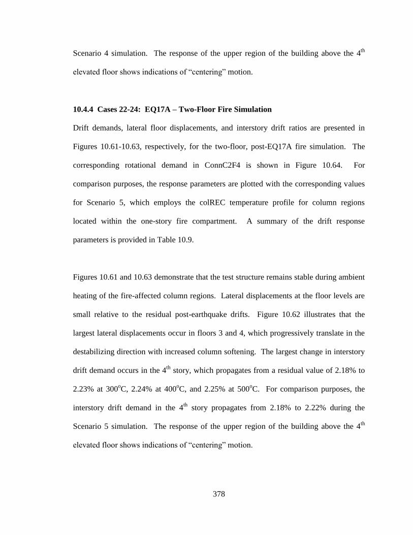
378
Scenario 4 simulation. The response of the upper region of the building above the 4th
elevated floor shows indications of “centering” motion.
10.4.4 Cases 22-24: EQ17A – Two-Floor Fire Simulation
Drift demands, lateral floor displacements, and interstory drift ratios are presented in
Figures 10.61-10.63, respectively, for the two-floor, post-EQ17A fire simulation. The
corresponding rotational demand in ConnC2F4 is shown in Figure 10.64. For
comparison purposes, the response parameters are plotted with the corresponding values
for Scenario 5, which employs the colREC temperature profile for column regions
located within the one-story fire compartment. A summary of the drift response
parameters is provided in Table 10.9.
Figures 10.61 and 10.63 demonstrate that the test structure remains stable during ambient
heating of the fire-affected column regions. Lateral displacements at the floor levels are
small relative to the residual post-earthquake drifts. Figure 10.62 illustrates that the
largest lateral displacements occur in floors 3 and 4, which progressively translate in the
destabilizing direction with increased column softening. The largest change in interstory
drift demand occurs in the 4th
story, which propagates from a residual value of 2.18% to
2.23% at 300oC, 2.24% at 400
oC, and 2.25% at 500
oC. For comparison purposes, the
interstory drift demand in the 4th
story propagates from 2.18% to 2.22% during the
Scenario 5 simulation. The response of the upper region of the building above the 4th
elevated floor shows indications of “centering” motion.

379
10.4.5 Discussion
The effect of temperature-induced column softening on sidesway response was
investigated by heating the column sections in the fire compartment to 300oC, 400
oC, and
500oC, which correspond to elastic modulus reductions of 20%, 30%, and 40%,
respectively (or kE,T of 80%, 70%, and 60%). Both single-floor and multi-floor fire
scenarios were evaluated. Temperature-induced column softening was shown to
significantly increase the flexibility of the moment-frame for lateral load response, and
resulted in considerable increases in interstory drift demand during the post-earthquake
fire simulations. However, because of the large stiffness requirements for seismic
performance, the heat-affected columns in the test structure retained considerable
bending resistance at the elevated temperatures investigated in the study. As a result, the
lateral floor displacements during the fire simulations were generally small relative to the
residual post-earthquake drifts. It is thought that a test structure designed for a smaller
seismic hazard, which uses thinner, more flexible column sections, may be more
susceptible to temperature-induced column softening during a post-earthquake fire.
10.5 SUMMARY
This chapter presented results from numerical simulations of sidesway response in the
test structure during post-earthquake fire exposure. The test program included six
conceptual post-earthquake fire simulations and a parametric study to identify potential
vulnerabilities related to temperature-induced beam hinge softening and temperature-
induced column softening.

380
The test structure remained stable during the single-floor and multi-floor post-earthquake
fire simulations with only small fluctuations in floor displacement. This was primarily
attributed to the high relative stiffness and thermal resistance of the insulated column
sections, and the substantial stiffness and strength of the heat-affected beam hinge
regions. Deformation response in the heat-affected stories and lower regions of the
building was generally influenced by destabilizing force demands, as evidenced by
progressive increases in interstory drift demand oriented in the destabilizing direction.
The upper region of the building tended to exhibit a “centering” response, likely driven
by elastic restoring forces and facilitated by the softened beam-column connections in the
heat-affected region. As expected, softening of beam-column connections along multiple
floor levels increased susceptibility to sidesway deformation and resulted in considerable
increases in interstory drift demand.
The limiting case where the heat-affected beams in the fire compartment no longer
restrain the rotations of the respective columns was investigated. As expected, loss of
rotational continuity at the beam-column connections significantly increased the
flexibility of the moment-frames for lateral load response, and resulted in considerable
increases in drift demand during the post-earthquake fire simulations.
The effect of temperature-induced column softening on sidesway response was also
investigated by heating the column sections in the fire compartment to 300oC, 400
oC, and
500oC, which correspond to elastic modulus reductions of 20%, 30%, and 40%.
Temperature-induced column softening was shown to significantly increase the flexibility

381
of the moment-frame for lateral load response, and resulted in considerable increases in
interstory drift demand during the post-earthquake fire simulations. However, because of
the large stiffness requirements for seismic performance, the heat-affected columns in the
test structure retained considerable bending resistance at the elevated temperatures
investigated in the study. As a result, the lateral floor displacements during the fire
simulations were generally small relative to the residual post-earthquake drifts.

Table 10.1 Drift demand relative to the residual post-earthquake geometry (Scenarios 1-6, fireLC-20min)
3rd Floor 4th Floor 5th Floor 3rd Story 4th Story 5th Story
1EQ11A / fireLCF3 /
bhFLEX / colREC0.0 0.0 0.0 0.00 0.00 -0.01 0.00
2EQ11A / fireLCF23 /
bhFLEX / colREC0.0 0.1 0.1 0.01 0.01 0.00 0.01
3EQ11A / fireLCF234 /
bhFLEX / colREC0.1 0.1 0.2 0.01 0.01 0.02 0.01
4EQ17A / fireLCF3 /
bhFLEX / colREC0.0 0.1 0.1 0.00 0.01 0.01 0.01
5EQ17A / fireLCF23 /
bhFLEX / colREC0.0 0.1 0.1 0.01 0.02 0.01 0.02
6EQ17A / fireLCF234 /
bhFLEX / colREC0.0 0.1 0.1 0.01 0.02 0.01 0.02
Scenario
No.ID
Lateral Displacement (cm)Absolute Change in
IDR Demand (%)
Absolute
Change in
Drift Index
for ConnC2F4
(%)
382

Table 10.2 Drift demand relative to the residual post-Earthquake geometry (Scenarios 1-6, fireLC-40min)
3rd Floor 4th Floor 5th Floor 3rd Story 4th Story 5th Story
1EQ11A / fireLCF3 /
bhFLEX / colREC0.0 0.1 0.0 0.01 0.00 -0.01 0.00
2EQ11A / fireLCF23 /
bhFLEX / colREC0.1 0.1 0.1 0.02 0.01 -0.01 0.01
3EQ11A / fireLCF234 /
bhFLEX / colREC0.1 0.2 0.3 0.02 0.02 0.03 0.02
4EQ17A / fireLCF3 /
bhFLEX / colREC0.1 0.2 0.2 0.01 0.02 0.01 0.02
5EQ17A / fireLCF23 /
bhFLEX / colREC0.1 0.2 0.3 0.02 0.03 0.01 0.03
6EQ17A / fireLCF234 /
bhFLEX / colREC0.1 0.2 0.3 0.02 0.03 0.01 0.03
Scenario
No.ID
Lateral Displacement (cm)Absolute Change in
IDR Demand (%)
Absolute
Change in
Drift Index
for ConnC2F4
(%)
383

Table 10.3 Drift demand relative to the residual post-earthquake geometry (Scenarios 1-6, fireLC-60min)
3rd Floor 4th Floor 5th Floor 3rd Story 4th Story 5th Story
1EQ11A / fireLCF3 /
bhFLEX / colREC0.1 0.1 0.0 0.01 0.00 -0.01 0.00
2EQ11A / fireLCF23 /
bhFLEX / colREC0.1 0.2 0.2 0.03 0.02 -0.01 0.02
3EQ11A / fireLCF234 /
bhFLEX / colREC0.1 0.3 0.5 0.03 0.04 0.05 0.04
4EQ17A / fireLCF3 /
bhFLEX / colREC0.1 0.2 0.3 0.02 0.03 0.02 0.03
5EQ17A / fireLCF23 /
bhFLEX / colREC0.1 0.3 0.4 0.03 0.05 0.02 0.05
6EQ17A / fireLCF234 /
bhFLEX / colREC0.1 0.3 0.4 0.03 0.05 0.02 0.05
Scenario
No.ID
Lateral Displacement (cm)Absolute Change in
IDR Demand (%)
Absolute
Change in
Drift Index
for ConnC2F4
(%)
384

Table 10.4 Drift demand relative to the residual post-earthquake geometry (Scenarios 1-3 & 7-9, fireLC-60min)
3rd Floor 4th Floor 5th Floor 3rd Story 4th Story 5th Story
1EQ11A / fireLCF3 /
bhFLEX / colREC0.1 0.1 0.0 0.01 0.00 -0.01 0.00
7EQ11A / fireLCF3 /
bhPIN / colREC0.0 -0.1 -0.3 0.00 -0.04 -0.05 -0.04
2EQ11A / fireLCF23 /
bhFLEX / colREC0.1 0.2 0.2 0.03 0.02 -0.01 0.02
8EQ11A / fireLCF23 /
bhPIN / colREC0.7 1.3 1.4 0.14 0.15 0.03 0.15
3EQ11A / fireLCF234 /
bhFLEX / colREC0.1 0.3 0.5 0.03 0.04 0.05 0.04
9EQ11A / fireLCF234 /
bhPIN / colREC1.4 3.7 6.2 0.29 0.54 0.62 0.54
Scenario
No.ID
Lateral Displacement (cm)Absolute Change in
IDR Demand (%)
Absolute
Change in
Drift Index
for ConnC2F4
(%)
385

Table 10.5 Drift demand relative to the residual post-earthquake geometry (Scenarios 4-6 & 10-12, fireLC-60min)
3rd Floor 4th Floor 5th Floor 3rd Story 4th Story 5th Story
4EQ17A / fireLCF3 /
bhFLEX / colREC0.1 0.2 0.3 0.02 0.03 0.02 0.03
10EQ17A / fireLCF3 /
bhPIN / colREC0.2 0.6 0.9 0.03 0.10 0.08 0.10
5EQ17A / fireLCF23 /
bhFLEX / colREC0.1 0.3 0.4 0.03 0.05 0.02 0.05
11EQ17A / fireLCF23 /
bhPIN / colREC0.9 2.2 2.9 0.18 0.32 0.17 0.32
6EQ17A / fireLCF234 /
bhFLEX / colREC0.1 0.3 0.4 0.03 0.05 0.02 0.05
12EQ17A / fireLCF234 /
bhPIN / colREC1.1 3.0 4.5 0.23 0.44 0.36 0.44
Scenario
No.ID
Lateral Displacement (cm)Absolute Change in
IDR Demand (%)
Absolute
Change in
Drift Index
for ConnC2F4
(%)
386

Table 10.6 Drift demand relative to the residual post-earthquake geometry (Scenarios 1 & 13-15, fireLC-60min)
3rd Floor 4th Floor 5th Floor 3rd Story 4th Story 5th Story
1EQ11A / fireLCF3 /
bhFLEX / colREC0.1 0.1 0.0 0.01 0.00 -0.01 0.00
13EQ11A / fireLCF3 /
bhFLEX / col3000.1 0.2 0.2 0.02 0.02 -0.01 0.02
14EQ11A / fireLCF3 /
bhFLEX / col4000.1 0.2 0.2 0.02 0.03 0.00 0.03
15EQ11A / fireLCF3 /
bhFLEX / col5000.1 0.3 0.3 0.02 0.04 0.00 0.04
Scenario
No.ID
Lateral Displacement (cm)Absolute Change in
IDR Demand (%)
Absolute
Change in
Drift Index
for ConnC2F4
(%)
387

Table 10.7 Drift demand relative to the residual post-earthquake geometry (Scenarios 2 & 16-18, fireLC-60min)
3rd Floor 4th Floor 5th Floor 3rd Story 4th Story 5th Story
2EQ11A / fireLCF23 /
bhFLEX / colREC0.1 0.2 0.2 0.03 0.02 -0.01 0.02
16EQ11A / fireLCF23 /
bhFLEX / col3000.1 0.3 0.3 0.03 0.03 0.00 0.03
17EQ11A / fireLCF23 /
bhFLEX / col4000.1 0.3 0.3 0.04 0.04 0.00 0.04
18EQ11A / fireLCF23 /
bhFLEX / col5000.2 0.4 0.4 0.04 0.06 0.00 0.06
Scenario
No.ID
Lateral Displacement (cm)Absolute Change in
IDR Demand (%)
Absolute
Change in
Drift Index
for ConnC2F4
(%)
388

Table 10.8 Drift demand relative to the residual post-earthquake geometry (Scenarios 4 & 19-21, fireLC-60min)
3rd Floor 4th Floor 5th Floor 3rd Story 4th Story 5th Story
4EQ17A / fireLCF3 /
bhFLEX / colREC0.1 0.2 0.3 0.02 0.03 0.02 0.03
19EQ17A / fireLCF3 /
bhFLEX / col3000.1 0.3 0.4 0.03 0.05 0.01 0.05
20EQ17A / fireLCF3 /
bhFLEX / col4000.2 0.4 0.4 0.03 0.06 0.01 0.06
21EQ17A / fireLCF3 /
bhFLEX / col5000.2 0.5 0.5 0.04 0.07 0.01 0.07
Scenario
No.ID
Lateral Displacement (cm)Absolute Change in
IDR Demand (%)
Absolute
Change in
Drift Index
for ConnC2F4
(%)
389

Table 10.9 Drift demand relative to the residual post-earthquake geometry (Scenarios 5 & 22-24, fireLC-60min)
3rd Floor 4th Floor 5th Floor 3rd Story 4th Story 5th Story
5EQ17A / fireLCF23 /
bhFLEX / colREC0.1 0.3 0.4 0.03 0.05 0.02 0.05
22EQ17A / fireLCF23 /
bhFLEX / col3000.2 0.4 0.5 0.04 0.05 0.02 0.05
23EQ17A / fireLCF23 /
bhFLEX / col4000.2 0.5 0.5 0.05 0.06 0.01 0.06
24EQ17A / fireLCF23 /
bhFLEX / col5000.2 0.5 0.6 0.06 0.07 0.01 0.07
Scenario
No.ID
Lateral Displacement (cm)Absolute Change in
IDR Demand (%)
Absolute
Change in
Drift Index
for ConnC2F4
(%)
390

391
Figure 10.1 Drift demands
Scenario 1: EQ11A / fireLCF3 / bhFLEX / colREC
Figure 10.2 Lateral floor displacements
Scenario 1: EQ11A / fireLCF3 / bhFLEX / colREC

392
Figure 10.3 Interstory drift demands
Scenario 1: EQ11A / fireLCF3 / bhFLEX / colREC
Figure 10.4 Rotational demand in ConnC2F4
Scenario 1: EQ11A / fireLCF3 / bhFLEX / colREC

393
Figure 10.5 Drift demands
Scenario 2: EQ11A / fireLCF23 / bhFLEX / colREC
Figure 10.6 Lateral floor displacements
Scenario 2: EQ11A / fireLCF23 / bhFLEX / colREC

394
Figure 10.7 Interstory drift demands
Scenario 2: EQ11A / fireLCF23 / bhFLEX / colREC
Figure 10.8 Rotational demand in ConnC2F4
Scenario 2: EQ11A / fireLCF23 / bhFLEX / colREC

395
Figure 10.9 Drift demands
Scenario 3: EQ11A / fireLCF234 / bhFLEX / colREC
Figure 10.10 Lateral floor displacements
Scenario 3: EQ11A / fireLCF234 / bhFLEX / colREC
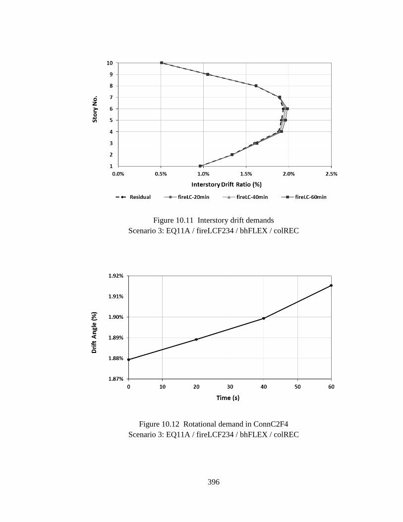
396
Figure 10.11 Interstory drift demands
Scenario 3: EQ11A / fireLCF234 / bhFLEX / colREC
Figure 10.12 Rotational demand in ConnC2F4
Scenario 3: EQ11A / fireLCF234 / bhFLEX / colREC

397
Figure 10.13 Drift demands
Scenario 4: EQ17A / fireLCF3 / bhFLEX / colREC
Figure 10.14 Lateral floor displacements
Scenario 4: EQ17A / fireLCF3 / bhFLEX / colREC

398
Figure 10.15 Interstory drift demands
Scenario 4: EQ17A / fireLCF3 / bhFLEX / colREC
Figure 10.16 Rotational demand in ConnC2F4
Scenario 4: EQ17A / fireLCF3 / bhFLEX / colREC

399
Figure 10.17 Drift demands
Scenario 5: EQ17A / fireLCF23 / bhFLEX / colREC
Figure 10.18 Lateral floor displacements
Scenario 5: EQ17A / fireLCF23 / bhFLEX / colREC

400
Figure 10.19 Interstory drift demands
Scenario 5: EQ17A / fireLCF23 / bhFLEX / colREC
Figure 10.20 Rotational demand in ConnC2F4
Scenario 5: EQ17A / fireLCF23 / bhFLEX / colREC
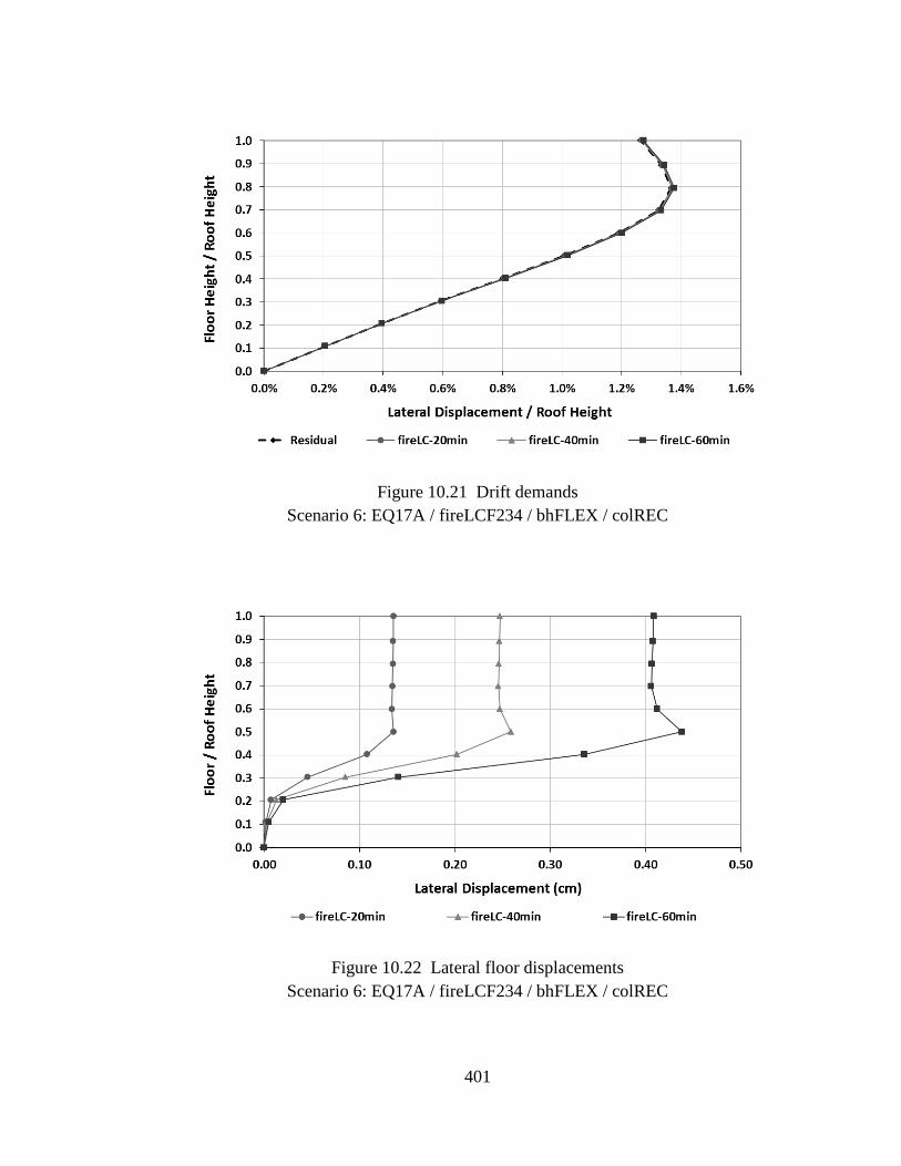
401
Figure 10.21 Drift demands
Scenario 6: EQ17A / fireLCF234 / bhFLEX / colREC
Figure 10.22 Lateral floor displacements
Scenario 6: EQ17A / fireLCF234 / bhFLEX / colREC

402
Figure 10.23 Interstory drift demands
Scenario 6: EQ17A / fireLCF234 / bhFLEX / colREC
Figure 10.24 Rotational demand in ConnC2F4
Scenario 6: EQ17A / fireLCF234 / bhFLEX / colREC

403
Figure 10.25 Drift demands
Scenario 7: EQ11A / fireLCF3 / bhPIN / colREC
Figure 10.26 Lateral floor displacements
Scenario 7: EQ11A / fireLCF3 / bhPIN / colREC

404
Figure 10.27 Interstory drift demands
Scenario 7: EQ11A / fireLCF3 / bhPIN / colREC
Figure 10.28 Rotational demand in ConnC2F4
Scenario 7: EQ11A / fireLCF3 / bhPIN / colREC

405
Figure 10.29 Drift demands
Scenario 8: EQ11A / fireLCF23 / bhPIN / colREC
Figure 10.30 Lateral floor displacements
Scenario 8: EQ11A / fireLCF23 / bhPIN / colREC

406
Figure 10.31 Interstory drift demands
Scenario 8: EQ11A / fireLCF23 / bhPIN / colREC
Figure 10.32 Rotational demand in ConnC2F4
Scenario 8: EQ11A / fireLCF23 / bhPIN / colREC

407
Figure 10.33 Drift demands
Scenario 9: EQ11A / fireLCF234 / bhPIN / colREC
Figure 10.34 Lateral floor displacements
Scenario 9: EQ11A / fireLCF234 / bhPIN / colREC

408
Figure 10.35 Interstory drift demands
Scenario 9: EQ11A / fireLCF234 / bhPIN / colREC
Figure 10.36 Rotational demand in ConnC2F4
Scenario 9: EQ11A / fireLCF234 / bhPIN / colREC
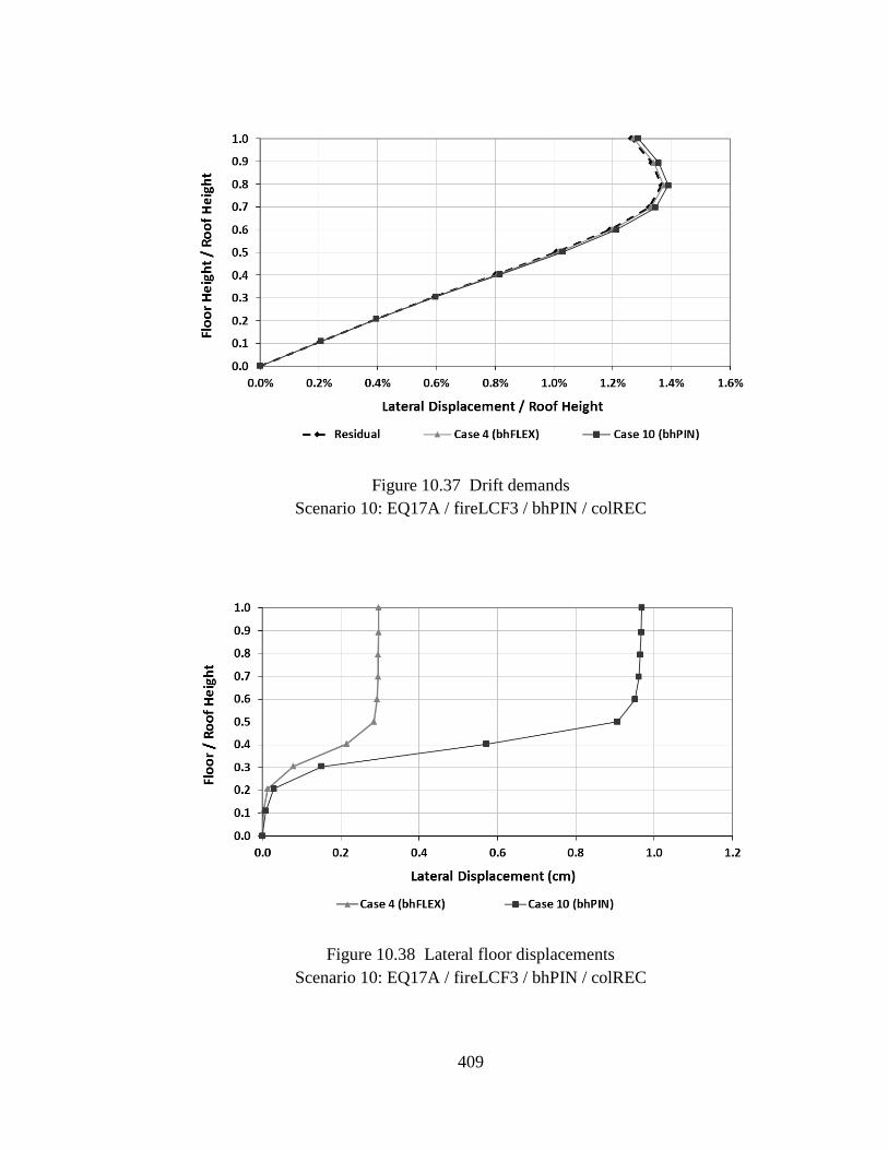
409
Figure 10.37 Drift demands
Scenario 10: EQ17A / fireLCF3 / bhPIN / colREC
Figure 10.38 Lateral floor displacements
Scenario 10: EQ17A / fireLCF3 / bhPIN / colREC

410
Figure 10.39 Interstory drift demands
Scenario 10: EQ17A / fireLCF3 / bhPIN / colREC
Figure 10.40 Rotational demand in ConnC2F4
Scenario 10: EQ17A / fireLCF3 / bhPIN / colREC

411
Figure 10.41 Drift demands
Scenario 11: EQ17A / fireLCF23 / bhPIN / colREC
Figure 10.42 Lateral floor displacements
Scenario 11: EQ17A / fireLCF23 / bhPIN / colREC

412
Figure 10.43 Interstory drift demands
Scenario 11: EQ17A / fireLCF23 / bhPIN / colREC
Figure 10.44 Rotational demand in ConnC2F4
Scenario 11: EQ17A / fireLCF23 / bhPIN / colREC

413
Figure 10.45 Drift demands
Scenario 12: EQ17A / fireLCF234 / bhPIN / colREC
Figure 10.46 Lateral floor displacements
Scenario 12: EQ17A / fireLCF234 / bhPIN / colREC

414
Figure 10.47 Interstory drift demands
Scenario 12: EQ17A / fireLCF234 / bhPIN / colREC
Figure 10.48 Rotational demand in ConnC2F4
Scenario 12: EQ17A / fireLCF234 / bhPIN / colREC

415
Figure 10.49 Drift demands
Scenarios 13-15: EQ11A / fireLCF3 / bhFLEX / col300-500
Figure 10.50 Lateral floor displacements
Scenarios 13-15: EQ11A / fireLCF3 / bhFLEX / col300-500

416
Figure 10.51 Interstory drift demands
Scenarios 13-15: EQ11A / fireLCF3 / bhFLEX / col300-500
Figure 10.52 Rotational demand in ConnC2F4
Scenarios 13-15: EQ11A / fireLCF3 / bhFLEX / col300-500

417
Figure 10.53 Drift demands
Scenario 16-18: EQ11A / fireLCF23 / bhFLEX / col300-500
Figure 10.54 Lateral floor displacements
Scenarios 16-18: EQ11A / fireLCF23 / bhFLEX / col300-500

418
Figure 10.55 Interstory drift demands
Scenarios 16-18: EQ11A / fireLCF23 / bhFLEX / col300-500
Figure 10.56 Rotational demand in ConnC2F4
Scenarios 16-18: EQ11A / fireLCF23 / bhFLEX / col300-500

419
Figure 10.57 Drift demands
Scenario 19-21: EQ17A / fireLCF3 / bhFLEX / col300-500
Figure 10.58 Lateral floor displacements
Scenario 19-21: EQ17A / fireLCF3 / bhFLEX / col300-500

420
Figure 10.59 Interstory drift demands
Scenario 19-21: EQ17A / fireLCF3 / bhFLEX / col300-500
Figure 10.60 Rotational demand in ConnC2F4
Scenarios 19-21: EQ17A / fireLCF3 / bhFLEX / col300-500

421
Figure 10.61 Drift demands
Scenarios 22-24: EQ17A / fireLCF23 / bhFLEX / col300-500
Figure 10.62 Lateral floor displacements
Scenarios 22-24: EQ17A / fireLCF23 / bhFLEX / col300-500

422
Figure 10.63 Interstory drift demands
Scenarios 22-24: EQ17A / fireLCF23 / bhFLEX / col300-500
Figure 10.64 Rotational demand in ConnC2F4
Scenarios 22-24: EQ17A / fireLCF23 / bhFLEX / col300-500

423
CHAPTER 11
SUMMARY, CONCLUSIONS, AND FUTURE WORK
11.1 OVERVIEW
The overarching objective of this research was to expand the knowledge base on the
behavior of steel moment-frame buildings during post-earthquake fire exposure. To this
end, this dissertation presents an analytical study on the thermomechanical response of
steel moment-frame beam-columns connections during post-earthquake fire exposure,
and addresses the potential vulnerability for steel moment-frame buildings associated
with sidesway instability due to temperature-induced moment-frame connection
softening. An analytical case study was developed for a representative steel moment-
frame office building located near coastal California. Forty-four nonlinear multi-degree-
of-freedom (MDOF) dynamic response history analyses were performed to characterize
force and deformation demands in the test structure and anticipated SFRM damage for
the maximum considered seismic hazard. A high-fidelity thermomechanical submodel
was developed for a representative moment-frame beam-column subassemblage to track
transient heat flow and moment-rotation response during two compartment fire
simulations. The moment-rotation response data from the submodel analyses was then
used to calibrate computationally efficient moment-frame beam-column connection
models for numerical simulations of global sidesway response during post-earthquake
fire exposure. The numerical simulations utilized a multi-step procedure to develop the
post-earthquake damaged state of the building, and to model the subsequent temperature-

424
induced degradation of the structural system during fire exposure. The objective of the
global simulation was to determine whether destabilizing forces in the system drive drift
demands in the heat-affected stories, due to temperature-induced softening of the
moment-frame beam-column connections; or whether elastic restoring forces, due to
residual plastic deformations, deform the softened beam hinge regions to relieve residual
stress demands. The test matrix for the study was designed to evaluate the performance
of the test structure for conceptual post-earthquake fire scenarios, thereby providing
representative case studies for evaluating the efficacy of existing building code
provisions for the multi-hazard scenario. Parametric sensitivity analyses were utilized to
identify potential vulnerabilities for future studies.
Section 11.2 summarizes the research tasks and observations from the study. The
conclusions drawn from the study are presented in Section 11.3. Finally, Section 11.4
proposes future experimental and analytical work.
11.2 SUMMARY
The following section provides a brief overview of the research tasks and observations
from the study. Conclusions drawn from the study are provided in Section 11.3.

425
11.2.1 Analysis and Design of the Ten-Story Steel Moment-Frame
Test Structure (Chapter 3)
A ten-story steel moment-frame analytical test structure was developed using
conventional methods of design and detailing. The test structure was representative
of a typical office building located near coastal California.
The lateral force resisting system for the test structure consisted of perimeter steel
special moment frames (SMF) with welded unreinforced flange – welded web
(WUF-W) beam-column connections. Performance requirements and detailing
standards for the frames were based on the guidelines of IBC-06 (IBC, 2006),
ASCE/SEI 7-05 (ASCE/SEI, 2005), and ANSI/AISC (2005a, 2005b, 2005c).
The design-basis seismic and wind hazards for the structure were determined based
on the guidelines of IBC-06 and ASCE/SEI 7-05. Lateral load analysis of the
building for seismic excitation utilized the equivalent lateral force (ELF) procedure of
ASCE/SEI 7-05.
The SMF design was driven by drift control requirements for seismic loading and
ductility requirements for the prequalified beam-column connections.
Fire protection for the building was achieved through a combination of active
suppression systems (e.g. automatic sprinklers) and augmentation of passive
resistance (e.g. thermal insulation) based on the prescriptive guidelines of IBC-06.
The SMF beams and columns were protected with 2-hour fire-rated dry-mix spray-
applied fire-resistive (SFRM) insulation.

426
11.2.2 Nonlinear MDOF Dynamic Response Model (Chapter 4)
A nonlinear MDOF dynamic response model for the test structure was developed in
the finite element software OpenSees (OpenSees, 2011) to study seismic response in
the N-S direction. Considering uncoupled unidirectional excitation, the structural
system was idealized as a half-system submodel composed of three integrated
analytical components: (1) a nonlinear SMF substructure used to model the lateral
load resistance provided by the typical N-S SMF; (2) a leaning column substructure
used to model tributary mass and second-order P-delta effects; and (3) a network of
equivalent viscous damping substructures used to model inherent (non-simulated)
energy-dissipation mechanisms in the structural system.
Inelastic response in the SMF hinge regions was modeled using nonlinear beam-
column elements with fiber section integration points. The uniaxial stress-strain
relation for the steel fibers was based on an expected (or probable) value for yield
stress and an idealized hardening model.
A flexible beam-column panel zone model was developed, using the approach
outlined in Charney and Downs (2004), to model web plate shear deformation and
flexural response in the column flanges.
A leaning column substructure was incorporated to model second-order P-delta
effects without overestimating the gravity forces acting on the lateral force resisting
system. Second-order effects were activated in the solution algorithm through
inclusion of the element geometric stiffness matrices.
Inherent (non-simulated) damping mechanisms in the system were modeled with a
network of calibrated viscous dashpot elements that proved a physical interpretation

427
of the global damping matrix. This approach was utilized to overcome numerical
difficulties with modeling mass and stiffness-proportional viscous damping in
nonlinear simulations, specifically the development of artificially large viscous forces
in cases where the global damping matrix and proportionality coefficients are not
updated during the simulation.
Gravity load demands for the dynamic simulation were based on the expected (or
probable) load case presented in FEMA P695 (FEMA, 2008).
The numerical time-stepping procedure for the simulation utilized the implicit
Newmark method with average acceleration. The incremental displacement vector
within each time step was determined using the modified Newton-Raphson iteration
method.
11.2.3 MCE Ground Motions (Chapter 5)
The spectral acceleration demand for the maximum considered seismic hazard was
developed using the guidelines of ASCE/SEI 7-05.
An ensemble of recorded ground motions from major seismic events was assembled
from the PEER-NGA database (PEER-NGA, 2011) using the guidelines in FEMA
P695.
Individual ground motion recordings were normalized with respect to peak ground
velocity (PGV) in order to remove unwarranted variability between records due to
inherent differences in event magnitude, site-source distance, source type, and site
conditions, while still maintaining the inherent aleatory (i.e., record-to-record)
variability necessary for characterizing the distribution in seismic response.

428
The normalized ground motion ensemble was then collectively scaled (using a
uniform scale factor) so that the median pseudo-acceleration response equaled the
prescriptive spectral acceleration demand from ASCE/SEI 7-05. Conceptually, this
approach envisioned the Far-Field record set as representative of a suite of records
from a major earthquake, in which individual records have some dispersion about an
expected value.
11.2.4 Response of the Test Structure for the MCE Hazard (Chapter 6)
A monotonic displacement-controlled (pushover) analysis was used to evaluate the
lateral strength and ductility of the test structure, and to quantify post-yield secant
stiffness for identification of problematic ground motion records (artificial loss of
transmissibility in the elongated period range due to low-frequency filtering).
Forty-four nonlinear response history analyses were performed to characterize force
and deformation demands in the test structure for the maximum considered seismic
hazard. Only one ground response record initiated sidesway collapse of the test
structure based on the collapse limits presented in Section 6.2.1.
Maximum interstory drift demands, measured in terms of an interstory drift ratio
(IDR), ranged from 1.3% to 4.9% with a median value of 2.8%. Residual IDR
demands in the test structure ranged from 0.1% to 3.9% with a median value of 1%.
Based on considerations of peak IDR demand (which can be related to anticipated
SFRM damage in SMF beam hinge regions), residual destabilizing moments were
recorded at the 4th
elevated floor. These moments ranged from 0.01% to 4.4% of the

429
base flexural capacity of the lateral force resisting system, with a median value of
0.6%.
Estimates of lateral load capacity, ductility, and peak roof drift demand for the ten-
story steel moment-frame test structure provided by the ELF procedure of ASCE/SEI
7-05 were found to correlate reasonably well with results from nonlinear MDOF
finite element analyses.
In order to evaluate earthquake-induced deformation demands in moment-frame
beam-column connections, a representative connection along the 4th
elevated floor
was selected based on considerations of drift demand and residual destabilizing
forces. Deformation response data was extracted from two nonlinear earthquake
simulations. Inelastic deformations were shown to concentrate, as intended, in the
beam hinge regions, while strain demands in the column and panel zone region
remained within the elastic range.
The frequency of exceedance was determined for potential interstory drift demands at
which damage to SFRM insulation in beam hinge regions might be expected. For
IDR demands of 2.5%, 2.75%, 3%, 3.25%, and 3.5%, the frequency of drift demand
exceedance was 57%, 41%, 25%, 23%, and 20%, respectively. It is also noted that
peak IDR demands in the test structure during MCE ground shaking frequently
concentrated along adjacent stories near the base of the structure, which can be
attributed to the dominance of the first mode of response. This poses a potential
vulnerability for a multi-floor post-earthquake scenario where temperature-induced
softening of beam hinge regions at successive floor levels (due to increased heat

430
penetration through the SFRM damage sites) effectively elongates the story height in
the sidesway frame.
11.2.5 Thermomechanical Beam-Column Connection Submodel (Chapter 7)
A high-fidelity moment-frame beam-column connection submodel was developed in
the nonlinear finite element software Abaqus (Abaqus, 2011) to study transient heat
flow and thermomechanical response during post-earthquake fire exposure. In order
to simplify the thermomechanical simulation, a one-way coupling methodology was
utilized, in which an uncoupled heat transfer simulation was used to drive a
dependent stress analysis.
Compartment fire models were developed from large-scale fire test data and available
literature regarding heat flux boundary conditions. Two ambient temperature records
from the 1993-1998 Cardington test program (British Steel, 1998, 1999) were
selected.
An idealized damage model for spray-applied fire-resistive material (SFRM) in
moment-frame beam hinge regions was developed based on the protected moment-
frame beam-column subassemblage tests reported by Braxtan and Pessiki (2009,
2011a, 2011b)
In-situ mechanical boundary condition models were developed to evaluate the
influence of restrained thermal expansion on moment-rotation response during fire
exposure.
A multi-step sequential analysis procedure was developed to simulate behavioral
response in the moment-frame beam-column subassemblage during seismic excitation

431
and post-earthquake fire exposure. The procedure was designed to transfer state data
between the analysis steps in order to capture the effect of residual deformations and
stress demands on structural response during thermal loading. Thermomechanical
properties for the various construction materials were developed from available
literature.
At selected time instances during the fire simulations, a displacement-controlled
(pushover) analysis was used to evaluate moment-rotation response the beam-column
subassemblage, independent of the actual external force demands.
11.2.6 Thermomechanical Beam-Column Connection Submodel
– Analytical Results (Chapter 8)
Steel temperatures in the fully insulated moment-frame beam-column subassemblage
remained below 300oC during the office and large compartment fire simulations. As
a result, temperature-induced degradation of the structural steel was minimal, and the
moment-rotation response of the beam-column subassemblage during fire exposure
was similar to the response at normal ambient temperature.
When idealized SFRM spall patterns were introduced in the moment-frame beam
hinge regions, representative of those reported by Braxtan and Pessiki (2009, 2011a,
2011b), temperatures in the exposed steel tracked closely with the ambient thermal
history of the fire simulation. The time lag between peak ambient temperature and
peak steel temperature was approximately 10-20min for the two fire scenarios
investigated in the study. Moderate increases in steel temperature were observed in

432
the lower regions of the beam web and web connection plate. Temperature increases
in the upper region of the beam hinge and beam-column panel zone were small.
Elastic modulus and yield stress of the exposed steel were reduced to 12% and 20%,
respectively, of their value at normal ambient temperature for the simulated office
fire, and to 28% and 43%, respectively, for the large compartment fire simulation. In
compression regions, this temperature-induced softening is exacerbated by the
presence of residual post-earthquake out-of-plane distortions. Reduced buckling
resistance of the heat-affected compression flange and web plate, as well as softening
of the heat-affected tensile region, lead to reductions in rotational stiffness of 30-50%
and a 20-30% reduction in flexural capacity.
11.2.7 Global Simulation of Sidesway Response during Post-Earthquake Fire
Exposure (Chapter 9)
A nonlinear numerical model and multi-step simulation process were developed
for evaluating global sidesway response during post-earthquake fire exposure.
Computationally efficient beam-column connection models were developed using
moment-rotation response data from the high-fidelity thermomechanical
submodel simulations of Chapter 7.
A pseudo-dynamic displacement-controlled procedure, based on response data
from the nonlinear dynamic analyses of Chapter 6, was utilized to simulate
seismic response of the test structure, with the objective of developing the post-
earthquake damaged condition.

433
A series of post-earthquake fire simulations were then performed by adjusting the
mechanical response of structural elements located within the fire compartment to
account for temperature effects. At selected time instances during the fire
simulation, large displacement static analyses were utilized to determine to the
transient state of equilibrium for the system.
The objective for the study was to determine whether second-order destabilizing
forces in the system drive rotational demands in the heat-affected connections and
drift demands in the system, or whether elastic restoring forces (due to residual
post-earthquake plastic deformations) deform the softened beam hinge regions to
relieve residual stress demands. The test matrix for the study was designed to
evaluate the performance of the test structure for a series of conceptual post-
earthquake fire scenarios, and to identify potential vulnerabilities through
parametric sensitivity analyses.
11.2.8 Global Simulation of Sidesway Response during Post-Earthquake Fire
Exposure – Analytical Results (Chapter 10)
The test structure remained stable during the single-floor and multi-floor post-
earthquake fire simulations with only small fluctuations in floor displacement.
Deformation response in the heat-affected stories and lower regions of the building
was generally influenced by destabilizing force demands, as evidenced by a
progressive increase in interstory drift demands oriented in the destabilizing direction.
The upper region of the building tended to exhibit a “centering” response, likely
driven by elastic restoring forces and facilitated by the softened beam-column

434
connections in the heat-affected region. As expected, softening of beam-column
connections along multiple floor levels increased susceptibility to sidesway
deformation and resulted in considerable increases in interstory drift demand.
The limiting case where the heat-affected beams in the fire compartment no longer
restrain the rotations of the respective columns was investigated. As expected, loss of
rotational continuity at the beam-column connections significantly increased the
flexibility of the moment-frames for lateral load response, and resulted in
considerable increases in drift demand during the post-earthquake fire simulations.
The effect of temperature-induced column softening on sidesway response was also
investigated by heating the column sections in the fire compartment to 300oC, 400
oC,
and 500oC, which correspond to elastic modulus reductions of 20%, 30%, and 40%,
respectively. Both single-floor and multi-floor fire scenarios were evaluated.
Temperature-induced column softening was shown to significantly increase the
flexibility of the moment-frame for lateral load response, and resulted in considerable
increases in interstory drift demand during the post-earthquake fire simulations.
11.3 CONCLUSIONS
The following section outlines the primary conclusions drawn from the study.
11.3.1 Damage to SFRM Insulation for Steel SMF during MCE Ground Shaking
The ductility requirements of ANSI/AISC (ANSI/AISC, 2005a, 2005b) ensure that
inelastic deformations in WUF-W steel SMF beam-column connections concentrate
in the beam hinge regions, while strain demands in the column and panel zone region

435
remain within the elastic range. In properly designed steel SMF, spalling of SFRM
insulation is likely limited to the beam hinge regions.
Peak rotational demands in steel SMF beam-column connections during MCE ground
shaking frequently exceed demands at which extensive yielding and buckling
distortions in the beam hinge regions are anticipated. Spalling of SFRM insulation in
SMF beam hinge regions is therefore anticipated during an MCE event.
Peak interstory drift demands during MCE ground shaking frequently concentrate in
adjacent stories due to the dominance of the first mode of response for low and mid-
rise SMF buildings. Spalling of SFRM insulation in SMF beam hinge regions is
therefore anticipated along multiple floor levels for an MCE event. This poses a
potential vulnerability for a multi-floor post-earthquake fire scenario where
temperature-induced softening of beam hinge regions at successive floor levels
effectively elongates the story height in the sidesway frame.
11.3.2 Effect of Earthquake-Induced Damage to SFRM Insulation in Moment-
Frame Beam Hinge Regions on Heat Penetration and Thermal Degradation
of Moment-Rotation Response during Post-Earthquake Fire Exposure
In an undamaged state, SFRM insulation provides considerable protection against
temperature-induced degradation of the structural steel, and the moment-rotation
response of the beam-column subassemblage during fire exposure is similar to the
response at normal ambient temperature.
Considering anticipated SFRM spall patterns, the study determined that steel
temperatures in the exposed flange regions track closely with the ambient thermal

436
history. The heat-affected flanges are subject to considerable thermal degradation,
e.g. 70-90% reductions in elastic modulus and 60-80% reductions in yield stress
were observed for the two fire scenarios investigated in the study. The heat-affected
zone, however, is localized near the SFRM damage site and only moderate increases
in steel temperature were observed in the lower regions of the beam web and web
connection plate. Temperature increases in the upper region of the beam hinge and
the beam-column panel zone are small.
Thermal degradation of the exposed flanges in the heat-affected beam hinge regions
can lead to considerable softening of moment-rotation response for the beam-column
subassemblage. Instantaneous rotational stiffness for the beam-column
subassemblage was reduced by 20-40% for the two fire scenarios investigated by the
study. At larger rotational demands, the secant stiffness for the beam-column
subassemblage was reduced by 35-50%. This softening is primarily attributed to
reduced buckling resistance in the heat-affected compression flange and web region,
and temperature-induced softening of the heat-affected tensile flange. Flexural
capacity for the beam-column subassemblage is also reduced by increased heat
penetration through the SFRM damage site, e.g. reductions of 20-30% were observed
for the two fire scenarios investigated in the study.
Mechanical restraint against thermal expansion significantly impacts the moment-
rotation response of the beam-column subassemblage during fire exposure. Higher
levels of restraint, provided by the surrounding structure, can significantly increase
compressive strain demands in the beam end regions and can exacerbate buckling
distortions in the heat-affected flanges. This can lead to pronounced softening of the

437
instantaneous rotational stiffness. The effect of mechanical restraint against thermal
expansion on the response of the connection at larger rotational demands is less
significant, and its influence on flexural capacity is negligible.
11.3.3 Sidesway Response of Steel Moment-Frame Buildings during
Post-Earthquake Fire Exposure
The ten-story steel moment-frame test structure investigated in this study remained
stable during the post-earthquake fire simulations with only small fluctuations in
lateral displacement. This was attributed to the robust moment-frame design driven
by stringent drift control and ductility requirements for seismic performance. These
requirements generally necessitate the use of deep beams and heavy column sections
in moment-frame designs. The large volume-to-surface area ratio of these heavy
column sections enhances their resistance to ambient heating and makes them less
susceptible to fire effects, especially assuming that the thermal insulation for the
columns is not damaged during seismic response. As a result, the moment-frame
columns provide considerable restraint against sidesway deformations in the system
during fire exposure, even with substantial temperature-induced softening of the
beam hinge regions along multiple floor levels. The considerable rotational stiffness
retained in the heat-affected beam hinge regions, due to limited heat penetration near
the damage sites, also provides a major contribution to the inherent resistance of
moment-frame buildings to sidesway deformations during post-earthquake fire
exposure.

438
Deformation response during post-earthquake fire exposure, particularly in the heat-
affected floors, is predominately governed by destabilizing force demands, although
“centering” behavior was frequently observed in the upper regions of the test
structure, which is indicative of the relative influence of elastic restoring forces.
The extent of temperature-induced beam hinge softening and temperature-induced
column softening were shown to have a significant effect on sidesway response
during fire exposure, and point to potential vulnerabilities for steel moment-frame
buildings that should be investigated in future studies. These effects are exacerbated
for the case of a multi-floor fire scenario where loss of rotational restraint along
successive floor levels increases the effective story height of the sidesway frame,
which can significantly increase susceptibility to sidesway deformation.
11.4 FUTURE WORK
This section identifies research tasks and areas (not covered in this dissertation) that will
further develop the knowledge base on the behavior of steel-framed buildings during
post-earthquake fire exposure. The following research tasks are recommended:
Large-scale experimental fire tests of steel moment-frame beam-column
subassemblages with damaged SFRM insulation to validate the heat transfer and
thermomechancal simulations performed in this dissertation, and to calibrate
parameters for improved numerical simulations of thermomechanical response.
Large-scale cyclic displacement-controlled tests of SFRM insulated gravity-frame
beam-column subassemblages to evaluate the seismic performance of thermal
insulation in gravity-frame beam-column connection regions.

439
If potential vulnerabilities for SFRM insulation in gravity-frame beam-column
connection regions are identified in the structural tests, a series of large-scale
thermomechanical tests are proposed to evaluate the influence of SFRM damage on
fracture of heat-affected gravity-frame beam-column connections and buckling of
heat-affected gravity columns, due to increased heat flow to the flange elements
through exposed steel at the SFRM damage sites.
Additional numerical studies of building response during post-earthquake fire
exposure, considering various building configurations, seismic hazard levels, and fire
exposure conditions. The interaction of temperature effects in the gravity frames,
floor system, and the lateral force resisting elements should be addressed, including
temperature-induced large displacement response in the floor system, temperature-
induced softening of moment-frame and gravity-frame beam-column connections,
and dynamic impact from falling debris.

440
REFERENCES
Abaqus v6.10, (2011). Dassault Systèmes, Providence, RI. (www.simulia.com).
AutoCAD v2010. (2011). Autodesk, San Rafael, CA. (www.autodesk.com).
Alemdar, B.N. and White, D.W. (2005). “Displacement, Flexibility, and Mixed Beam-
Column Finite Element Formulations for Distributed Plasticity Analysis”, Journal of
Structural Engineering, American Society of Civil Engineers, Vol. 131, No. 12,
December, pp. 1811-1819.
ANSI/AISC 341-05: Seismic Provisions for Structural Steel Buildings. (2005a). American
Institute of Steel Construction, Chicago, IL.
ANSI/AISC 358-05: Prequalified Connections for Special and Intermediate Steel Moment
Frames for Seismic Applications. (2005b) American Institute of Steel Construction,
Chicago, IL.
ANSI/AISC 360-05: Specification for Structural Steel Buildings. (2005c). American
Institute of Steel Construction, Chicago, IL.
ASCE/SEI 7-05: Minimum Design Loads for Buildings and Other Structures. (2005).
American Society of Civil Engineers, Reston, VA.
ASTM A992/A992M-11. (2011). American Society of Testing and Materials (ASTM),
West Conshohocken, PA.
ASTM E119-00a: Standard Test Methods for Fire Tests of Building Construction and
Materials. (2000a). American Society of Testing and Materials (ASTM), West
Conshohocken, PA.
ASTM E736-00: Standard Test Method for Cohesion/Adhesion of Sprayed Fire-Resistive
Materials Applied to Structural Members. (2000b). American Society of Testing and
Materials (ASTM), West Conshohocken, PA.
Bathe, K.J. (2006). Finite Element Procedures. Prentice Hall, Pearson Education, Inc.,
Upper Saddle River, NJ.
Bejan, A. (1993). Heat Transfer, John Wiley & Sons, New York, NY.

441
Braxtan, N.L. (2009). “Post-Earthquake Fire Performance of Steel Moment-Frame
Building Columns”, PhD Dissertation, Department of Civil and Environmental
Engineering, Lehigh University, Bethlehem, PA.
Braxtan, N.L. and Pessiki, S. (2011a), “Bond Performance of SFRM on Steel Plates
Subjected to Tensile Yielding”, Journal of Fire Protection Engineering, Vol. 21(1),
pp. 37-55.
Braxtan, N.L. and Pessiki, S. (2011b), “Postearthquake Fire Performance of Sprayed
Fire-Resistive Material on Steel Moment Frames”, Journal of Structural Engineering,
American Society of Civil Engineers, Vol. 137, No. 9, pp. 946-953.
Brewster, M.Q. (1992). Thermal Radiative Transfer and Properties, John Wiley & Sons,
New York, NY.
British Steel. (1998) “The Behavior of a Multi-Storey Steel Framed Building Subjected
to Fire Attack – Experimental Data”, STC Technical Report, Swinden Technology
Centre, Rotherham, South Yorkshire, UK.
British Steel. (1999). “The Behavior of Multi-Storey Steel Framed Buildings in Fire”,
(1999). STC Technical Report, Swinden Technology Centre, Rotherham, South
Yorkshire, UK.
Buchanan, A. (2002). Sturctural Design for Fire Safety. John Wiley & Sons, New York,
NY.
California Building Code. (2010). California Building Standards Commission,
Sacramento, CA.
Charney, F.A. (2008). “Unintended Consequences of Modeling Damping in Structures”,
Journal of Structural Engineering, American Society of Civil Engineers, Vol. 134,
No. 4, April, pp. 581-592.
Charney, F.A. (2010). Seismic Loads – Guide to the Seismic Load Provisions of ASCE
7-05, American Society of Civil Engineers, Reston, VA.
Charney, F. A. and Downs, W. M. (2004). “Modeling procedures for panel zone
deformations in moment resisting frames”, Proceedings from International
Conference on Connections in Steel Structures, Amsterdam, Denmark, June 3-4.

442
Cheney, W. and Kincaid, D. (2008). Numerical Mathematics and Computing (6th
Ed.).Thomson Higher Education, Belmont, CA.
Cook, R.D., Malkus, D.S., Plesha, M.E., and Witt, R.J. (2002). Concepts and
Applications of Finite Element Analysis (4th
Ed.). Wiley, New York, NY.
Corte, G.D. , Landolfo, R., and Mazzolani, F.M. (2003) “Post-earthquake fire resistance
of moment resisting steel frames”, Fire Safety Journal, International Association for
Fire Safety Science, Vol. 38, No. 7, November, pp. 593-612.
Cousins, W.J. and Smith, W.D. (2004). “Estimated Losses due to Post-Earthquake Fire in
Three New Zealand Cities”, Proceedings from 2004 NZSEE Conference, Rototua,
New Zealand.
Drysdale, D. (1998). An Introduction to Fire Dynamics (2nd
Ed.). John Wiley & Sons,
Chichester, UK.
EC1: Actions on Structures – Part 1.2: General Actions – Actions on Structures Exposed
to Fire. (2002). British Standards Institution, London, UK.
EC2: Design of Concrete Structures – Part 1.2: General Actions – Structural Fire
Design. (1996). British Standards Institution, London, UK.
EC3: Design of Steel Structures – Part 1.2: General Actions – Structural Fire Design.
(2001). British Standards Institution, London, UK.
European Space Agency (2011). IMPRESS Education Site, Paris, France,
(www.spaceflight.esa.int/impress/text/education/index.html).
Faggiano, B. (2007) “Fire after earthquake”, Proceedings from WG1 Meeting on Urban
Habitat Constructions under Catastrophic Event, Prague, Czech Republic, March
30-31.
Faggiano B., Esposto M., Mazzolani F.M., and Landolfo R. (2007). “Fire Analysis on
Steel Portal Frames Damaged After Earthquake According to Performance Based
Design”, Proceedings from WG1 Meeting on Urban Habitat Constructions under
Catastrophic Event, Prague, Czech Republic, March 30-31.
FEMA 350: Recommended Seismic Design Criteria for New Steel Moment-Frame
Buildings. (2000). Federal Emergency Management Agency, Washington, D.C.

443
FEMA 461: Interim Testing Protocols for Determining the Seismic Performance
Characteristics of Structural and Nonstructural Components. (2007). Federal
Emergency Management Agency, Washington, D.C.
FEMA P695: Quantification of Building Seismic Performance Factors. (2008). Federal
Emergency Management Agency, Washington, D.C.
Holman, J.P. (2010). Heat Transfer (10th
Ed.), McGraw Hill, New York, NY.
International Building Code. (2006). International Code Council, Inc., Country Club
Hills, IL.
Isolatek International Product Manual. (2011). Isolatek International, Stanhope, NJ.
Jiaru, Q., Haiqun, Y., Feng, Y., Hai, D., Jianhua, L., andYueming, L. (2005).
“Experimental Study of Full-Scale Steel Beam-to-Column Moment Connections”,
Journal of Earthquake Engineering and Engineering Vibration, Vol. 5, No. 2, pp.
311-323.
Keller, W. J. and Pessiki, S. (2011a). “Nonlinear Dynamic Response of a Ten-Story Steel
Moment-Frame Test Structure for the Maximum Considered Seismic Hazard”, ATLSS
Report No. 11-06, Center for Advanced Technology for Large Structural Systems,
Lehigh University, Bethlehem, PA.
Keller, W.J. and Pessiki, S. (2011b). “Thermomechanical simulation of post-earthquake
fire exposure in a ten-story steel moment-frame test structure”, ATLSS Report No.
11-07, Center for Advanced Technology for Large Structural Systems, Lehigh
University, Bethlehem, PA.
Kelly, E.J. and Tell, R.N. (2011). “Modeling the Number of Ignitions Following an
Earthquake: Developing Prediction Limits for Overdispersed Count Data”, Technical
Report No. LA-UR-11-01857, Los Alamos National Laboratory, Los Alamos, NM.
Krawinkler, H. (1978). “Shear in Beam-Column Joints in Seismic Design of Frames”,
Engineering Journal, Vol. 15, No. 3, American Institute of Steel Construction,
Chicago, IL.
McGuire, W., Gallagher, R.H., and Ziemian, R.D. (2000). Matrix Structural Analysis (2nd
Ed.). John Wiley & Sons, Inc., New York, NY.

444
Lamont, S. (2001). “The Behaviour of Multi-Storey Composite Steel Framed Structures
in Response to Compartment Fires”, PhD Dissertation, Department of Civil and
Environmental Engineering, University of Edinburgh, Edinburgh, Scotland.
Lamont, S., Usmani, A.S., and Drysdale, D.D. (2001). “Heat Transfer Analysis of the
Composite Slab in the Cardington Frame Fire Tests”, Fire Safety Journal, Vol. 36,
November, pp. 815-839.
Lee, B. J., Pessiki, S., and Kohno, M. (2006). “Analytical investigation of steel column
fire tests”, ATLSS Report No. 06-23, Center for Advanced Technology for Large
Structural Systems, Lehigh University, Bethlehem, PA.
Lee, S. and Davidson, R. (2010). “Application of a Physics-Based Simulation Model to
Examine Post-Earthquake Fire Spread”, Journal of Earthquake Engineering, Vol. 14,
pp.688-705.
Lie, T.T. (1992). Structural Fire Protection - ASCE Manual and Reports on Engineering
Practice No. 78, American Society of Civil Engineers, New York, NY.
Logan, D.L. (2007). A First Course in the Finite Element Method. Thomson Learning,
Tampa, FL.
Mroz, J. (1967). “On the Description of Anisotropic Workhardening”, Journal of the
Mechanics and Physics of Solids, Vol. 15, Issue 3, pp. 163-175.
Neuenhofer, A. and Filippou, F.C. (1997). “Evaluation of Nonlinear Frame Finite-
Element Models”, Journal of Structural Engineering, American Society of Civil
Engineers, Vol. 123, No. 7, July, pp. 958-966.
Neuenhofer, A. and Filippou, F.C. (1998). “Geometrically Nonlinear Flexibility-Based
Frame Finite Element”, Journal of Structural Engineering, American Society of Civil
Engineers, Vol. 124, No. 6, June, pp. 704-711.
Newman, G.M., Robinson, J.T., and Bayley, C.G. (2000) Fire Safe Design: A New
Approach to Multi-Storey Steel-Framed Buildings, The Steel Construction Institute,
Sheffield, UK.
NIST NCSTAR 1-3D: Mechanical Properties of Structural Steel, Federal Building and
Fire Safety Investigation of the of the Work Trade Center Disaster. (2005). National
Institute of Standards and Technology, Gaithersburg, MD.
NFPA 909: Standard for the Protection of Cultural Resources. (1997). National Fire
Protection Association, Quincy, MA.

445
OpenSees v2.2, Open System for Earthquake Engineering Simulation, Pacific Earthquake
Engineering Research Center, University of California Berkeley, USA, 2011.
(www.opensees.berkeley.edu)
PEER-NGA Strong Ground Motion Database. (2011). (www.peer.berkeley.edu/nga/)
Ren, A.Z. and Xie, X.Y. (2004) “The simulation of post-earthquake fire-prone area
based on GIS”, Journal of Fire Sciences, Vol. 22, No. 5, September, pp.421-439.
Roke, D. (2010) “Damage-free seismic-resistant self-centering concentrically-braced
frames”, PhD Dissertation, Department of Civil and Environmental Engineering,
Lehigh University, Bethlehem, PA.
Scawthorn, C.R. (2008). “Fire Following Earthquake - The ShakeOut Scenario Report”,
SPA Technical Report, SPA Risk, LLC, Berkeley, CA.
Scott, M. H. and Fenves, G.L. (2006). “Plastic hinge integration methods for force-based
beam-column elements”, Journal of Structural Engineering, American Society of
Civil Engineers, Vol. 132, No. 2, pp. 244-252.
SFPE Handbook on Fire Protection Engineering (1st Ed.). (1988). National Fire
Protection Association, Quincy, MA.
Siegel, R. and Howell, J.R. (1980). Thermal Radiation Heat Transfer (2nd
Ed.),
Hemisphere Publishing Co., Washington, D.C.
Spacone, E., Ciampi, V., and Filippou, F.C. (1992). “A Beam Element for Seismic
Damage Analysis”, Technical Report No. UCB/EERC-92/07, Earthquake
Engineering Research Center, University of California, Berkeley.
Taucer, F.F., Spacone, E., and Filippou, F.C. (1991). “A Fiber Beam-Column Element
for Seismic Response Analysis of Reinforced Concrete Structures”, Technical Report
No. UCB/EERC-91/17, Earthquake Engineering Research Center, University of
California, Berkeley.
The SFPE Task Group on Fire Exposures to Structural Elements. (2004). Society for Fire
Protection Engineering (SFPE), Bethesda, MD.
Thomas, B.G. and Finney, R.L. (1984). Calculus and Analytic Geometry. Addison-
Wesley, Reading, MA.
Wang, Y.C. (2002). Steel and Composite Structures: Behavior and Design for Fire
Safety, Spon Press, New York, NY.

446
Yassin, H., Iqbal, F., Bagchi, A., and Kodur, V.K.R. (2008) “Assessment of post-
earthquake fire performance of steel-frame buildings”, Proceedings from 14th
World
Conference on Earthquake Engineering, Beijing, China, Oct. 12-17.
Zeris, C.A. and Mahin, S.A. (1988). “Analysis of Reinforced Concrete Beam-Columns
under Uniaxial Excitation”, Journal of Structural Engineering, American Society of
Civil Engineers, Vol. 114, pp. 804-820.
Zeris, C.A. and Mahin, S.A. (1991). “Behavior of Reinforced Concrete Structures
Subjected to Biaxial Excitation”, Journal of Structural Engineering, American
Society of Civil Engineers, Vol. 117, pp. 2657-2673.

447
APPENDIX 1
ISOLATEK BLAZE SHIELD II
SPRAY-APPLIED FIRE-RESISTIVE INSULATION
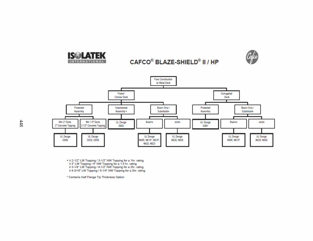
448

449

450

451

452

453

454

455
APPENDIX 2
IMPLICIT NEWMARK TIME-STEPPING PROCEDURE
FOR NONLINEAR DYNAMIC ANALYSIS
The following section presents the implicit Newmark two-parameter time-stepping
procedure, assuming average acceleration over the time step (γ = 1/2 and β = 1/4), for
nonlinear dynamic analysis. The algorithm utilizes the modified Newton-Raphson
iteration scheme to determine the incremental displacement vector within each time step.
The governing equation of motion for the problem is presented in Equation A2-1.
(Equation A2-1)
Where
m is the mass matrix for the MDOF dynamic system
c is the damping matrix for the MDOF dynamic system
k is the tangent stiffness matrix for the MDOF dynamic system at time t
is a vector of accelerations for the dynamic DOF at time t
is a vector of velocities for the dynamic DOF at time t
is a vector of displacements for the dynamic DOF at time t
is a vector of ground accelerations at the support nodes at time t
is the ground displacement influence vector for the MDOF dynamic system

456
The time-stepping method is initialized by setting time t =0 and solving Equation A2-1
for the initial acceleration vector ( ).
Solve: ( ) for (Equation A2-2)
Where
is the external force vector at t =0; equal to
( ) is the restoring force vector at t =0; equal to
The time increment Δt is then selected to ensure accuracy of solution and numerical
stability. It is noted that the Newmark method with average acceleration is
unconditionally numerically stable, so the time step is selected for compatibility with the
ground motion record (to ensure an accurate representation of the ground acceleration
history) and to facilitate convergence of the numerical solution.
Integration constants and are then determined using Equations A2-3 and A2-4.
( ⁄ ) (Equation A2-3)
(Equation A2-4)
The numerical time-stepping procedure then performs the following calculations at each
time step i:
1. (Equation A2-5)
2. Determine the tangent stiffness matrix, (see note 1 below)
3. ( ⁄ ) [ ( ) ⁄ ] (Equation A2-6)

457
4. Solve for from and (see note 2 below)
5. ( ⁄ ) (Equation A2-7)
6. [ ( ) ⁄ ] ( ⁄ ) (Equation A2-8)
7. (Equation A2-9)
8. (Equation A2-10)
9. (Equation A2-11)
Where
is the incremental external force vector at the end of time step i;
equal to
is the incremental displacement vector for the MDOF dynamic system at the
end of time step i
is the incremental acceleration vector for the MDOF dynamic system at the
end of time step i
is the accumulated displacement vector for the MDOF dynamic system at the
end of time step i
is the accumulated velocity vector for the MDOF dynamic system at the end
of time step i
is the accumulated acceleration vector for the MDOF dynamic system at the
end of time step i

458
Note 1: The numerical procedures for state determination and formulation of the element
tangent stiffness matrix (Step 2 in the incremental time-stepping procedure) are
dependent on element type.
Note 2: Step 4, which determines the incremental displacement vector , requires an
iterative procedure within the time step in order to reduce the error introduced by the use
of the tangent stiffness matrix ( ) instead of the unknown secant stiffness matrix ( ).
In the modified Newton-Raphson method, the tangent stiffness matrix is calculated at
time i, the beginning of the time step, and is used through all iterations within that time
step. Thus the matrix needs to be factorized only once, and is used repeatedly during
the iteration process. This method is usually preferred over the Newton-Raphson
method, where the matrix is updated for each iteration cycle. It is noted that updating
of the tangent stiffness matrix for each iteration cycle improves numerical convergence
but can add significant computational effort. The procedure for the modified Newton-
Raphson iteration method is as follows, where the superscript j indicates the iteration
number within the time step:
The Newton-Raphson iteration is initialized at j =0.
1. ( )
(Equation A2-12)
2. ( ) ( ) (Equation A2-13)
3. ( ) (Equation A2-14)
4. (Equation A2-15)

459
Where
is the accumulated displacement vector for the MDOF dynamic system at the
end of time step i
( )
is the accumulated displacement vector for the MDOF dynamic system at
time step i+1, at the initialization step of the Newton-Raphson iteration (j=0)
( ) is the accumulated restoring force vector for the MDOF dynamic system at
the end of time step i
( )
is the accumulated restoring force vector for the MDOF dynamic system at
the initialization step of the Newton-Raphson iteration (j=0)
is the parameter defined in Equation 4-5 calculated at the end of time step i
( ) is the incremental residual force vector for the MDOF dynamic system at
the first Newton-Raphson iteration (j = 1)
is the parameter defined in Equation 4-6 calculated at the end of time step i
is the matrix (related to tangent stiffness) for the Newton-Raphson iteration
The following calculations are then performed for each iteration, j = 1,2,3,…
1. Solve ( ) ( ) for ( ) (Equation A2-16)
2. ( )
( )
( ) (Equation A2-17)
3. ( ) ( )
( ) ( )
( ) (Equation A2-18)
4. ( ) ( ) ( ) (Equation A2-19)

460
Iteration within the time step terminates when the condition in Equation A2-20 is
satisfied, or the number of iterations exceeds a prescribed threshold value.
[ ( )] ( )
[ ]
(Equation A2-20)
Where
is a prescribed tolerance for convergence
In this criterion the work done by the residual forces ( ( )) through the displacement
increments ( ( )) is compared to the work associated with total incremental (over the
time step) force ( ) and the current estimate of the total incremental displacement
( ).

461
APPENDIX 3
NONLINEAR FLEXIBILITY-BASED
FIBER BEAM-COLUMN ELEMENT
A3.1 OVERVIEW
The following section presents the formulation and implementation of a nonlinear
flexibility-based fiber beam-column element, similar to the one utilized in the earthquake
simulations of Chapter 6. The notation and methodology have been reproduced from
Taucer et al. (1991).
A3.2 GENERALIZED FORCES AND DEFORMATIONS
The generalized forces and deformations at the element and section levels for a beam
subject to bi-axial bending and axial extension are presented in Figure A3.1. The
parameters can be grouped in the following vectors:
{ } (Equation A3-1)
{ } (Equation A3-2)
Where
is the element force vector
, , , and are bending moments at the element end nodes
is the axial force
is the element deformation vector
, , , and are rotations relative to the chord at the element end nodes
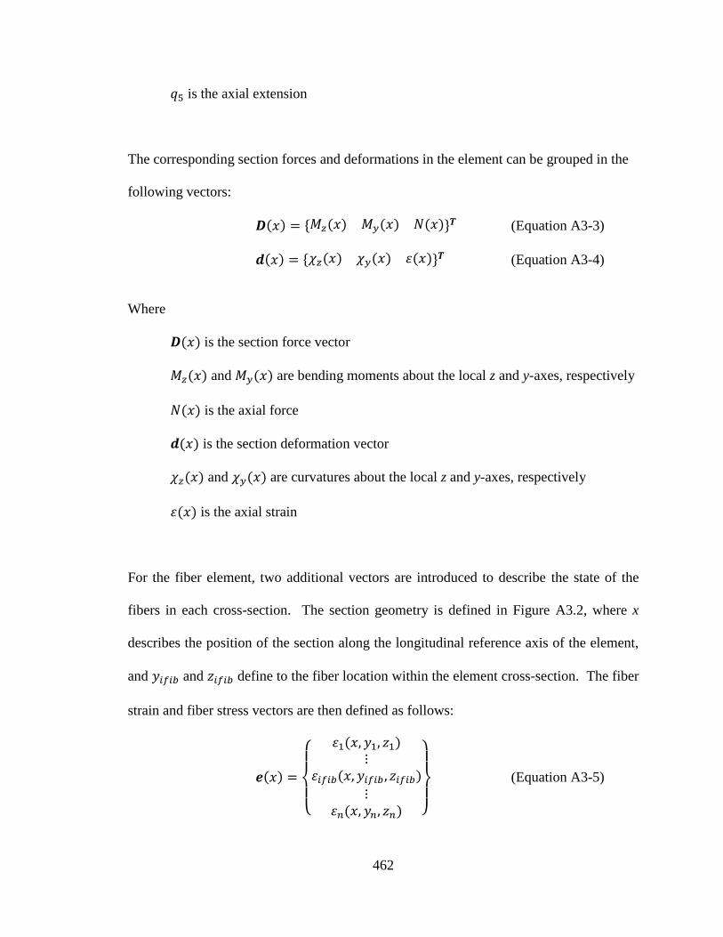
462
is the axial extension
The corresponding section forces and deformations in the element can be grouped in the
following vectors:
( ) { ( ) ( ) ( )} (Equation A3-3)
( ) { ( ) ( ) ( )} (Equation A3-4)
Where
( ) is the section force vector
( ) and ( ) are bending moments about the local z and y-axes, respectively
( ) is the axial force
( ) is the section deformation vector
( ) and ( ) are curvatures about the local z and y-axes, respectively
( ) is the axial strain
For the fiber element, two additional vectors are introduced to describe the state of the
fibers in each cross-section. The section geometry is defined in Figure A3.2, where x
describes the position of the section along the longitudinal reference axis of the element,
and and define to the fiber location within the element cross-section. The fiber
strain and fiber stress vectors are then defined as follows:
( )
{
( )
( )
( ) }
(Equation A3-5)

463
Where
( ) is the fiber strain vector
( ) is the uniaxial strain in fiber i, located at ( ) within
the element cross-section, at location x along the member length.
( )
{
( )
( )
( ) }
(Equation A3-6)
Where
( ) is the fiber stress vector
( ) is the uniaxial stress in fiber i, located at ( ) within
the element cross-section at location x along the member length.
Assuming that plane sections remain plane and normal to the longitudinal axis, the fiber
strain vector and the section deformation vector can be related as follows:
( ) ( ) ( ) (Equation A3-7)
where ( ) is a linear geometric matrix, referred to as the compatibility matrix:
( )
[
]
(Equation A3-8)
A summary of the vectors and matrices defining state parameters at the structure,
element, section, and fiber levels is provided in Figure A3.3.
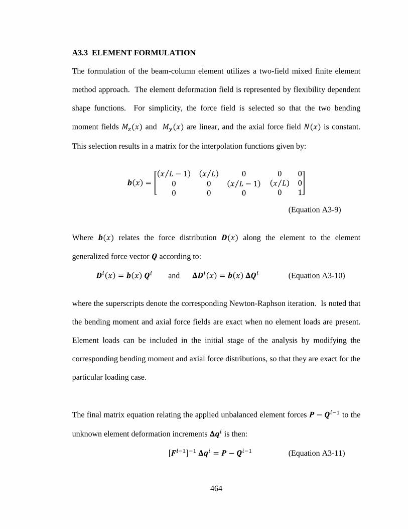
464
A3.3 ELEMENT FORMULATION
The formulation of the beam-column element utilizes a two-field mixed finite element
method approach. The element deformation field is represented by flexibility dependent
shape functions. For simplicity, the force field is selected so that the two bending
moment fields ( ) and ( ) are linear, and the axial force field ( ) is constant.
This selection results in a matrix for the interpolation functions given by:
( ) [( ⁄ ) ( ⁄ )
( ⁄ )
( ⁄ )
]
(Equation A3-9)
Where ( ) relates the force distribution ( ) along the element to the element
generalized force vector according to:
( ) ( ) and ( ) ( ) (Equation A3-10)
where the superscripts denote the corresponding Newton-Raphson iteration. Is noted that
the bending moment and axial force fields are exact when no element loads are present.
Element loads can be included in the initial stage of the analysis by modifying the
corresponding bending moment and axial force distributions, so that they are exact for the
particular loading case.
The final matrix equation relating the applied unbalanced element forces to the
unknown element deformation increments is then:
[ ] (Equation A3-11)

465
A3.4 STATE DETERMINATION
At the i-th Newton-Raphson iteration it is necessary to determine the element resisting
forces for the current element deformations. When the section force-deformation relation
is explicitly known, the new tangent stiffness ( ) can be directly computed for the
given section forces ( ) and deformations ( ), where j represents the element
iteration within the Newton-Raphson iteration cycle. In the case of the fiber model,
however, the geometric matrix ( ) is first used to obtain the fiber strain increments for
the given deformation increments ( ), following the assumption that plane sections
remain plane and normal to the longitudinal axis.
( ) ( ) ( ) (Equation A3-12)
The fiber strains are then updated to the new value:
( ) ( ) ( ) (Equation A3-13)
The new stress
and tangent modulus
of all fibers are determined from the
appropriate fiber stress-strain relation. The fiber stresses are then grouped in vector
and the tangent moduli are written in a diagonal matrix
. By defining a diagonal
matrix A, which contains entries of the fiber areas , and using the section
compatibility matrix ( ), the new section tangent stiffness matrix is determined as:
( ) ( )( ) ( ) (Equation A3-14)

466
which reduces to:
( )
[
∑
( )
∑
( )
∑
( )
∑
( )
∑
( )
∑
( )
∑
( )
∑
( )
∑
( )
]
(Equation A3-15)
The new section tangent stiffness matrix ( ) is then inverted to obtain the new section
tangent flexibility matrix ( ). Since the section resisting forces ( ) cannot be
obtained directly from the section force-deformation relation, they are determined by
summation of the axial force and biaxial bending contribution of all fibers as follows:
( ) ( ) (Equation A3-16)
which reduces to
( )
{
∑
( )
∑
( )
∑
( )
}
(Equation A3-17)

467
A3.5 NUMERICAL IMPLEMENTATION
The numerical procedure for incorporating the nonlinear fiber beam-column element in a
conventional finite element is provided below. The steps of the algorithm are illustrated
schematically in Figures A3.4-A3.7.
Step 1: Start the analysis
Initiate load step 1; Set k = 1.
Step 2: Start the Newton-Raphson iteration cycle
Initiate Newton-Raphson iteration 1; Set i = 1.
Step 3: Solve the global system of equations and update the structure displacement
increments
Using the unbalanced force vector ( )
and the structure tangent stiffness matrix
( )
from the previous Newton-Raphson iteration (i-1), the change in the structure
displacement increments ( ) is computed from the solution of the linear system of
equations:
( )
( ) ( ) (Equation A3-18)
The unbalanced force vector ( )
is obtained as the difference between total applied
loads and total resisting forces at the conclusion of the previous iteration (i-1) in Step 19.
When k = 1 and i = 1, then ( )
, where is the incremental external force
vector for the first load step (k = 1). The tangent stiffness matrix ( )
is based on the

468
state of the structure at the end of the previous Newton-Raphson iteration and is
determined in Step 18. When i = 1, two possible conditions exist:
k = 1: The initial tangent stiffness is determined by imposing a very small
deformation increment on the sections of all elements. The fiber material modules
return the initial tangent modulus of elasticity from which the section, element,
and, finally, the structure stiffness is assembled.
k > 1: The structure stiffness is equal to the tangent stiffness at the end of the
previous load step (k-1), that is ( )
;
Once the unbalanced force vector ( )
and tangent stiffness matrix ( )
have
been determined, the change in structure displacement increments ( ) is calculated
using Equation A3-18. This vector is then added to the displacement increments
( ) at the end of the previous Newton-Raphson iteration (i-1) to obtain the
displacement increments ( ) for the present Newton-Raphson iteration ( i ), as shown
in Equation A3-19.
( ) ( ) ( ) (Equation A3-19)
It is noted that when i = 1, ( ) is initialized to zero.
Step 4: Compute the element deformation increments
Using the compatibility matrix the change in the element deformation increments
( ) is computed from the structure displacement increments ( ) , as shown in
Equation A3-20.
( ) ( ) (Equation A3-20)

469
where is a geometric matrix that relates global displacements to element
displacements. The element deformation increments are then updated for the present
Newton-Raphson iteration ( i ), as shown in Figure A3-21:
( ) ( ) ( ) (Equation A3-21)
When i = 1, ( ) is initialized to zero. It is noted that the element displacement
increments do not change during the element iteration loop (counted in j iterations).
Step 5: Start the element state determination
Initiate element iteration 1; Set j=1.
Step 6: Compute the change in the element force increments
Two cases are possible:
j = 1: (( ) ) is obtained from the change in the element displacement
increments ( ) for the current Newton-Raphson iteration ( i ) using the element
tangent stiffness matrix ( ) at the end of the previous Newton-Raphson iteration
(i-1):
(( ) ) ( ) ( ) (Equation A3-22)
j > 1: (( ) ) is obtained from the residual element deformations (( ) )
at
the end of the previous Newton-Raphson iteration (j-1) and the corresponding
element stiffness matrix (( ) )
:
(( ) ) (( ) )
(( ) )
(Equation A3-23)

470
Step 7: Update the element force increments and the element resisting forces
With the change in the element force increments (( ) ) known, the element force
increments are updated for the present element iteration ( j ):
(( ) ) (( ) )
(( ) )
(Equation A3-24)
When i = 1 and j = 1, (( ) ) is initialized to zero.
The current element resisting forces are then obtained by adding the element force
increments (( ) ) to the resisting force vector at the end of the previous
(converged) load step (k-1):
(( ) ) (( ) )
(Equation A3-25)
Step 8: Compute the section force increments
The change in the section force increments (( ( )) ) is computed with the
interpolation function b(x), and the corresponding force increments are updated for the
present element iteration ( j ):
(( ( )) ) ( )(( ) )
(Equation A3-26)
(( ( )) ) (( ( )) )
(( ( )) )
(Equation A3-27)
When i = 1 and j = 1, (( ( )) ) is initialized to zero. The section forces are then
updated according to Equation A-28.
(( ( )) ) ( ) (( ( )) )
(Equation A3-28)
When k = 1, ( )

471
Step 9: Compute the change in section deformation increments
The change in section deformation increments (( ( )) ) is obtained by adding the
effect of the change in section force increments (( ( )) ) to the residual section
deformations at the end of the previous element iteration (j-1):
(( ( )) ) (( ( )) )
(( ( )) )
(( ( )) )
(Equation A3-29)
When j = 1, (( ( )) )
The section deformation increments are then updated accordingly:
(( ( )) ) (( ( )) )
(( ( )) )
(Equation A3-30)
When i = 1 and j = 1, (( ( )) )
Step 10: Compute the fiber deformation increments
The change in fiber deformation increments is computed with the section compatibility
matrix l(x) and the deformation increments are updated:
(( ( )) ) ( )(( ( )) )
(Equation A3-31)
(( ( )) ) (( ( )) )
(( ( )) )
(Equation A3-32)
The fiber deformations are then updated according to Equation A3-33:
(( ( )) ) ( ) (( ( )) )
(Equation A3-33)
When i = 1 and j = 1, (( ( )) )

472
Step 11: Compute fiber stresses and update the tangent modulus of the fibers
For the current fiber deformations (( ( )) ) the fiber material modules return the new
fiber stresses (( ( )) )
and the updated tangent stiffness modulus of the
fibers (( ( ))
)
.
Step 12: Compute the section tangent stiffness and flexibility matrices
The updated tangent modulus of the fibers (( ( ))
)
is used in the
calculation of the current section tangent stiffness matrix:
(( ( )) )
[
∑ ( )
( )
∑ ( )
( )
∑ ( )
( )
∑ ( )
( )
∑ ( )
( )
∑ ( )
( )
∑ ( )
( )
∑ ( )
( )
∑ ( )
( )
]
(Equation A3-34)
where
( ) (( ( ))
)
(Equation A3-35)
and n(x) is the total number of fibers in the section. The section stiffness matrix is then
inverted to yield the current section flexibility matrix:
(( ( )) ) [(( ( )) )
]
(Equation A3-36)

473
Step 13: Compute the section resisting forces
The section resisting forces are computed by summation of the axial force and biaxial
bending moment contributions of all fibers:
(( ( ))
)
[ ∑ (( ( ))
)
( )
∑ (( ( )) )
( )
∑ (( ( )) )
( )
]
(Equation A3-37)
Step 14: Compute the section unbalanced forces
The section unbalanced forces are computed as the difference between applied loads and
resisting forces:
(( ( ))
)
(( ( )) ) ((
( )) )
(Equation A3-38)
It is noted that the unbalanced force vector should be checked to see if satisfies the
specified section tolerance.
Step 15: Compute the residual section deformations
Given the unbalanced section force vector (( ( ))
)
, the residual section
deformations are calculated according to Equation A3-39.
(( ( )) ) (( ( )) )
((
( )) )
(Equation A3-39)

474
Step 16: Compute the element flexibility and stiffness matrices
The element flexibility matrix is obtained by numerical integration of section flexibilities:
(( ) ) ∑ [
( ) (( ( ))
)
( )]
(Equation A3-40)
where m is the number of monitored sections in the beam-column element, xnsec is the x-
coordinate of the section in the local reference system, and wnsec is the corresponding
weight factor.
The element stiffness matrix is then obtained by inverting the flexibility matrix:
(( ) ) [(( ) )
]
(Equation A3-41)
Step 17: Check for element convergence
Element convergence is achieved when all section unbalanced forces satisfy the specified
section tolerance. Two cases are possible:
If convergence is achieved, then go to Step 18
If convergence is not achieved then compute the residual element deformations, as
shown in Equation A3-42. Increment j by 1 and return to Step 6.
(( ) ) ∑ [
( ) (( ( ))
)
]
(Equation A3-42)

475
Step 18: Compute the structure resisting forces and update the structure stiffness
matrix
When all elements have converged, the i-th Newton-Raphson iteration is complete. The
structure resisting forces ( ) are determined by assembly of all element resisting
forces ( ) according to the expression:
( ) ∑
( )
(Equation A3-43)
The structure tangent stiffness matrix is updated by assembly of the element stiffness
matrices:
( ) ∑
( )
(Equation A3-44)
Step 19: Compute the structure unbalanced forces
The structure unbalanced forces ( ) are calculated as the difference between total
applied loads and total resisting forces (
) :
( )
( ) (Equation A3.45)
where is determined from the total applied load at the end of the previous load step
(k-1) and the current load increment:
(Equation A3.46)
For k = 1,

476
Step 20: Check for structure convergence
If the unbalanced forces at the structure level satisfy the specified tolerance, convergence
is achieved. Two cases are possible:
If convergence is not achieved, increment i by 1, and return to Step 3 to start the next
Newton-Raphson iteration;
If convergence is achieved, load step k is complete. Go to Step 21.
Step 21: Update force and deformation vectors and start new load step
All force and deformation vectors are updated by adding the vector increments for load
step k to the corresponding total forces and deformations at the end of the previous load
step (k-1):
(Equation A3.47)
( ) ( ) ( ) (Equation A3.48)
( ) ( ) ( ) (Equation A3.49)
Update ( ) to ( )
( ) ( ) ( ) (Equation A3.50)
At this point, two cases are possible:
k = kn. The entire external load PE was applied and the analysis is complete.
k < kn. Increment k by 1. Compute the new structure unbalanced force vector.
( )
(Equation A3.51)
and return to Step 2.

477
Figure A3.1 Generalized forces and deformations at the
element and section level (from Taucer et al. 1991)
Figure A3.2 Fiber section geometry (from Taucer et al. 1991)

478
Figure A3.3 Vectors and matrices defining state parameters at the
structure, element, section, and fiber levels (from Taucer et al. 1991)
Figure A3.4 Example of force-displacement history
at the structure level (from Taucer et al. 1991)

479
Figure A3.5 Example of force-deformation history
at the element level (from Taucer et al. 1991)
Figure A3.6 Example of force-deformation history
at the section level (from Taucer et al. 1991)

480
Figure A3.7 Example of force-deformation history
at the fiber level (from Taucer et al. 1991)

481
APPENDIX 4
THE FINITE ELEMENT METHOD FOR
THREE-DIMENSIONAL STEADY-STATE AND TRANSIENT
HEAT TRANSFER ANALYSIS
The following section provides an overview of the finite element method for three-
dimensional heat transfer analysis. The numerical procedure is developed for a 20-node
hexahedral continuum finite element, which is similar to the Abaqus DC3D20 element
utilized in the study. The element conduction matrix is developed using the
isoparametric formulation.
Step 1: Select the Element Type
The 20-node hexahedral continuum finite element is presented in Figure A4.1 in global
(x, y, z) and natural, or intrinsic, (s, t, z’) coordinates. The element has 1-DOF (scalar
value of temperature) at each node. The natural coordinate system is normalized by the
respective element dimension in each direction, and ranges from -1 to 1 with respect to
the origin, which is located at the centroid of the element. For example, the natural
coordinates for corner nodes 3 and 8 (as shown in Figure A5.1) are (-1, 1, -1) and
(1, 1, 1), respectively.
Step 2: Select the Element Temperature Function
Since the element has 20-nodal DOF (1-DOF per node), and therefore 20-boundary
equations, a single polynomial function utilizing 20-terms can be selected to model the

482
temperature distribution within the continuum. It is noted that the terms of the function
are selected so that they do not bias a particular direction, and that the temperature
function is similar to the corresponding shape function developed for the 20-node finite
element, refer to the 20-node stress analysis element in Appendix A5.
( )
(Equation A4-1)
or in matrix form:
( ) { }
{
}
(Equation A4-2)
Alternatively, Equation A4-2 can be expressed in terms of the nodal temperatures:
{
}
[
]
{
}
(Equation A4-3)

483
Equation A4-3 contains a system of 20-equations (one for each nodal DOF, Ti=1…20) with
20-unknowns ( ). For example, at corner node i=1, where , and
:
( )
( ) ( ) ( ) ( )( ) ( )( )
( )( ) ( ) ( ) ( ) ( ) ( )
( )( ) ( ) ( ) ( )( ) ( ) ( )
( )( ) ( )( )( ) ( ) ( )( )
( )( ) ( ) ( )( )( )
(Equation A4-4)
The constants are then determined, in terms of the nodal temperatures, by multiplying the
inverse of the shape function matrix with the nodal temperature vector, as shown in
Equation A4-5.
{
}
[
]
{
}
(Equation A4-5)

484
Once the constants have been expressed in terms of the nodal temperatures, the
temperature function from Equation A4-2 can be re-formulated as:
( ) { }
{
}
( )
(Equation A4-6)
where are geometric shape functions that relate the temperature at a point within
the continuum to the nodal temperatures, considering the position of the point with
respect to the natural coordinate system. Letting , , for corner nodes i = 1,
2,…, 8 (as shown in Figure A4.1), the shape function can be expressed as:
( )( )( )
(
)
(Equation A4-7)
For example, at corner node i = 1, where , and :
( )( )( )
( )
(Equation A4-8)

485
For the midside nodes at i = 17, 18, 19, 20, where , , , the shape
function is expressed as:
( )( )( )
(Equation A4-9)
For the midside nodes at , , (i = 10, 12, 14, 16), the shape
functions are:
( )( )( )
(Equation A4-10)
Finally, for the midside nodes at , , (i = 9, 11, 13, 15), the shape
functions are:
( )( )( )
(Equation A4-11)
Step 3: Define the Temperature Gradient-Temperature and Heat Flux-
Temperature Gradient Relationships
The temperature gradient vector, in global coordinates, which is analogous to the strain
vector used in the stress analysis problem, is presented in Equation A4-12.

486
{
}
(Equation A4-12)
Because the temperature gradients in Equation A4-12 are expressed in terms of global
coordinates (x, y, z), and the temperature function in Equation A4-6 is expressed in terms
of the natural coordinate system (s, t, z’), the chain rule of differentiation is utilized:
(Equations A4-13a-c)
In Equations A4-13a-c,
( ⁄ ) ( ⁄ ) ( ⁄ ) ( ⁄ ) ( ⁄ ) ( ⁄ ) ( ⁄ ) ( ⁄ )
and ( ⁄ ) are determined from Equation A5-6 of Appendix A5.
( ⁄ ) ( ⁄ ) and ( ⁄ ) are determined from Equation A4-6.
( ⁄ ) ( ⁄ ) and ( ⁄ ) are unknown.

487
Equations A4-13a-c are then solved for ( ⁄ ) ( ⁄ ) and ( ⁄ ) using Cramer’s
rule as follows:
|
|
|
|
| |
|
|
|
|
| |
|
|
|
|
| |
(Equations A4-14a-c)
Where | | is the determinant of the Jacobian matrix, and is equal to:
[
]
(Equation A4-15)

488
Evaluating the determinant of the numerators in Equations A4-14a-c produces the
following relations:
|
|
|
|
(
) [(
) (
) (
) (
)] (
) [(
) (
) (
) (
)]
(
) [(
) (
) (
) (
)]
|
|
|
|
(
) [(
) (
) (
) (
)] (
) [(
) (
) (
) (
)]
(
) [(
) (
) (
) (
)]

489
|
|
|
|
(
) [(
) (
) (
) (
)] (
) [(
) (
) (
) (
)]
(
) [(
) (
) (
) (
)]
(Equations A4-16a-c)
The temperature gradient-temperature relation then becomes:
| |{
( ) ( )
( )
}
( )
(Equation A4-17)
Where
( ) ( ( )
) [(
) (
) (
) (
)] (
) [(
( )
) (
) (
) (
( )
)]
(
) [(
( )
) (
) (
) (
( )
)]
( ) (
) [(
( )
) (
) (
) (
( )
)] (
( )
) [(
) (
) (
) (
)]
(
) [(
) (
( )
) (
( )
) (
)]

490
( ) (
) [(
) (
( )
) (
( )
) (
)] (
) [(
) (
( )
) (
( )
) (
)]
( ( )
) [(
) (
) (
) (
)]
(Equations A4-18a-c)
Considering Equation A4-6, Equation A5-17 can be restructured as:
(Equations A4-19)
Where
is an operator matrix, equal to:
| |{
( ) ( )
( )
}
(Equations A4-20)
Multiplication of the operator matrix and the shape function matrix then
yields the temperature gradient-temperature matrix :
(Equations A4-21)
Where
(Equations A4-22)

491
Equation A4-22 is the temperature gradient-temperature relation for the heat transfer
analysis.
The heat flux-temperature gradient relation is developed by considering Fourier’s law of
heat conduction:
,
, and
(Equations A4-23a-c)
Where
and represent the heat conducted into the continuum (or control volume) at
the boundary surfaces in x, y, z-directions, respectively, as illustrated in Figure
A4.2.
and represent the thermal conductivity of the material in the x, y, and z-
directions, respectively.
In matrix form, the heat flux-temperature gradient relation becomes:
{
}
(Equation A4-24)

492
or, considering Equation A4-22:
(Equation A4-25)
Where is material property matrix, calculated as:
[
]
(Equation A4-26)
Step 4: Derive the Element Heat Transfer Equations
The element heat transfer equations are derived through minimization of the heat transfer
functional, as discussed in Logan (2007). It is noted that all of the terms in the derivation
reference the global coordinate system (x, y, z). The functional describing heat transfer
can be expressed as:
(Equation A4-27)

493
Where
∭
(Equation A4-28)
∭
(Equation A4-29)
∬
(Equation A4-30)
∬ (
)
(Equation A4-31)
is the temperature gradient vector defined in Equation A4-22.
is the material matrix defined in Equation A4-26.
is the nodal temperature vector defined in Equation A4-3.
is the shape function vector defined in Equation A4-6.
is a scalar quantity representative of the heat generated (positive value) or lost.
(negative value) within the solid body.
is a scalar quantity representative of the heat flow to the surface of the solid body
(e.g. radiative heat transfer from a thermal source).
is a scalar quantity representative of the convective heat transfer coefficient (film
conductance).

494
is a scalar quantity representative of the ambient fluid temperature.
V is the control volume.
Sq* is the boundary surface involved in radiative heat transfer.
Sh is the boundary surface involved in convective heat transfer.
Considering Equation A4-22 and the fact that the nodal temperatures are independent of
the general coordinates, the functional becomes:
∭
∭
∬
∬ [
(
) ]
(Equation A4-32)
The functional is then minimized with respect to the nodal temperature vector , as
shown in Equation A4-33:
∭
∭
∬
∬ ∬
(Equation A4-33)

495
Equation A4-33 can be restructured as:
(Equation A4-34)
Where
is the conduction matrix, equal to:
[∭
∬
]
(Equation A4-35)
is a vector that represents an internal heat source (positive) or sink (negative),
equal to:
∭
(Equation A4-36)
is a vector that represents the heat flux into the boundary surface, equal to:
∬
(Equation A4-37)
is a vector that represents the heat transfer due to convection, equal to:
∬
(Equation A4-38)

496
Equations A4-35 through A4-38 present the element conduction matrix and heat source
vectors as formulated in global coordinates (x, y, z). For the isoparametric formulation,
however, the matrices and are functions of the natural coordinates (s, t, z’).
In order to transform the variables and region from global (x, y, z) to natural (s, t, z’)
coordinates, the following theorem is utilized:
∬ ( )
∭ ( )| |
∭ ( )
∭ ( )| |
(Equations A4-39a-b)
Where
[
]
[
]
The mathematical proof for the theorem is provided in Thomas and Finney (1984).

497
Using the relations in Equations A4-39a-b, the element conduction matrix and heat
source vectors are determined for the isoparametric formulation as follows:
∫ ∫ ∫ | |
∬ | |
(Equation A4-40)
∫ ∫ ∫
| |
(Equation A4-41)
∬
| |
(Equation A4-42)
∬
| |
(Equation A4-43)
where Sh and Sq* are defined in terms of the natural coordinate system.
Integration of the terms in Equations A4-40 to A4-43 is accomplished using a numerical
procedure, as illustrated below for the conductive matrix (excluding the second term
related to convective heat transfer, for simplicity).
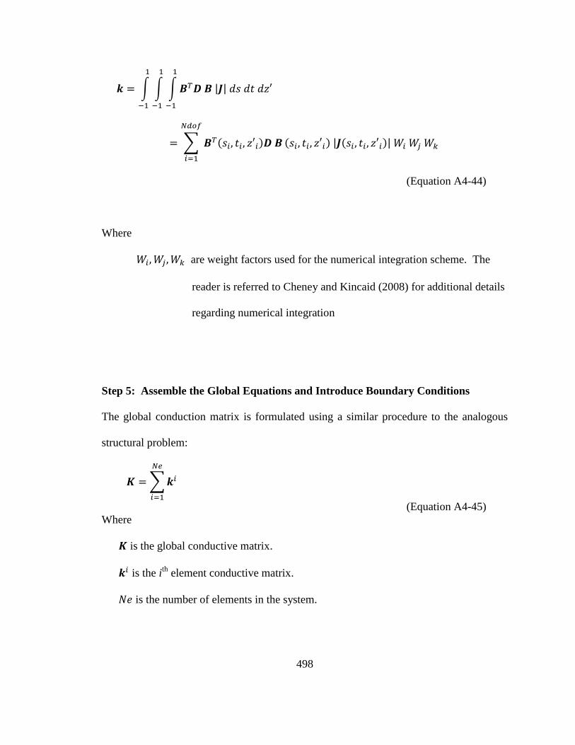
498
∫ ∫ ∫ | |
∑ ( )
( ) | ( )|
(Equation A4-44)
Where
are weight factors used for the numerical integration scheme. The
reader is referred to Cheney and Kincaid (2008) for additional details
regarding numerical integration
Step 5: Assemble the Global Equations and Introduce Boundary Conditions
The global conduction matrix is formulated using a similar procedure to the analogous
structural problem:
∑
(Equation A4-45)
Where
is the global conductive matrix.
is the ith
element conductive matrix.
is the number of elements in the system.

499
Similarly, the global heat source vector is assembled from the element heat source
vectors:
∑
(Equation A4-46)
Where
is the global heat source vector.
represents the ith
element heat source vector.
is the number of force vectors in the system.
The global system of equations for heat transfer analysis then takes the form:
(Equation A4-47)
Boundary conditions for the analysis are imposed by specifying known nodal temperature
values and heat flux boundaries (Equation A4-42 for radiative heat transfer and Equation
A4-43 for convective heat transfer). The system of equations in Equation A4-32
therefore contains both known and unknown nodal temperatures and heat flows
Step 6: Solve for the Nodal Temperatures
Since the system of equations contains nonzero values at prescribed DOF
(nonhomogeneous system of equations), a numerical procedure referred to as the penalty
method is used to solve for the unknown values. The penalty method is easy to

500
implement in a computer program and is discussed in Section 2.5 and Appendix B.4 of
Logan (2007).
Step 7: Solve for the Element Temperature Gradients and Heat Fluxes
Once the element nodal temperatures have been determined from Step 6, the element
temperature gradients are determined from Equation A4-22. The element
temperature gradients are then used to determine the element heat fluxes using
Equation A4-25.
Time-Dependent Heat Transfer
Transient, or time-dependent, heat transfer can be considered by replacing in Equation
A4-29 with:
(Equation A4-48)
Where
is a scalar quantity representative of the heat generated (positive value) or lost.
(negative value) within the solid body.
is the mass density of the material.
is the specific heat of the material.
is the time rate of change in temperature.

501
The term in Equation A4-29 then becomes:
∭
(
)
∭
(Equation A4-49)
Minimization of the functional with respect to the nodal temperature vector yields:
∭
∭
(Equation A4-50)
The integrand in the second term in Equation A4-50 is analogous to the consistent-mass
matrix in the structural dynamics problem, and can be denoted as:
global formulation,
∭
isoparametric formulation,
∫ ∫ ∫ | |
(Equation A4-51a-b)

502
The element equilibrium equations then become:
(Equation A4-52)
The corresponding global equilibrium equations are:
(Equation A4-53)
In a similar manner to the analogous structural dynamics problem, a numerical time-
stepping procedure is used to evaluate Equation A4-53, an example of which is provided
below. The reader is referred to Cheney and Kincaid (2008) for additional details
regarding numerical solution methods for the transient heat transfer problem.
Using the generalized trapezoid rule, the temperature states at time i and at time
i+1 can be related by:
[( ) ]( )
(Equation A4-54)
Much like Newmark’s method for numerical time integration of the second-order
equations of structural dynamics, Equation A4-54 includes a parameter that is chosen
by the user. Various numerical integration methods result, depending on the value of :

503
= 0: Forward difference, or Euler, which is conditionally stable according to
Equation A4-55.
( )
(Equation A4-55)
Where is the largest eigenvalue of:
( ) (Equation A4-56)
( ) (Equation A4-57)
= 1/2: Crank-Nicolson, or trapezoid, rule, which is unconditionally stable. It is
noted that if = 1/2 and sharp transients exist, this method may generate spurious
oscillations in the solution (Logan, 2007).
= 2/3: Galerkin, which is unconditionally stable.
= 1: Backward difference, which is unconditionally stable.
It is noted that if = 0, the numerical integration method is explicit, i.e. can be
solved using only state data at time t = i, as shown in Equation A4-62. If > 0, the
integration method is implicit because it utilizes state data from t = i and t = i+1 to solve
for . The use of > 1/2 along with a small time increment is recommended by
Logan (2007).

504
Once a value for has been selected, Equation A4-53 can be written for time instances i
and i+1, where the first equation is multiplied by ( ) and the second equation is
multiplied by :
( ) ( ) ( )
(Equation A4-58)
( ) ( )
(Equation A4-59)
Adding Equations A4-58 and A4-59 yields:
[( ) ] [( ) ] ( )
(Equation A4-60)
Using Equation A4-54, the time derivative terms can be eliminated, and Equation A4-60
becomes:
( )
[( ) ] ( )
(Equation A4-61)

505
which can be restructured as:
(
) (
( ) ) ( )
(Equation A4-62)
A summary of the numerical time-stepping procedure used to solve for the nodal
temperature vector T is provided below:
The nodal temperature vector is initialized at
(known initial conditions ).
At the first time increment , Equation A4-62 is solved for using
.
The process is repeated for subsequent time instances, where the previous nodal
temperature distribution is used to solve for the new nodal temperature
distribution in Equation A4-62.

506
Figure A4.1 20-node quadratic hexahedral continuum finite element:
global coordinates (x, y, z) and natural, or intrinsic, coordinates (s, t, z’)
(from Logan (2007))
Figure A4.2 Three-dimensional heat transfer boundary conditions
(from Logan (2007))

507
APPENDIX 5
THE FINITE ELEMENT METHOD FOR
THREE-DIMENSIONAL STRESS ANALYSIS
CONSIDERING THERMAL STRAIN
The following section provides an overview of the finite element method for three-
dimensional stress analysis, considering thermal strain. The numerical procedure is
developed for a 20-node hexahedral continuum finite element, which is similar to the
Abaqus C3D20 element utilized in the study. The element stiffness matrix is developed
using the isoparametric formulation.
Step 1: Select the Element Type
The 20-node hexahedral continuum finite element is presented in Figure A5.1 in global
(x, y, z) and natural, or intrinsic, (s, t, z’) coordinates. The element has 3-displacement
DOF (ui, vi, wi) at each node, where u, v, and w are the displacements in the global x, y,
and z-directions, respectively. The natural coordinate system is normalized by the
respective element dimension in each direction, and ranges from -1 to 1 with respect to
the origin, which is located at the centroid of the element. For example, the natural
coordinates for corner nodes 3 and 8 (as shown in Figure A5.1) are (-1, 1, -1) and
(1, 1, 1), respectively.

508
Step 2: Select the Element Displacement Functions
Since the element has 60-nodal DOF (3-DOF per node), and therefore 60-boundary
equations, three polynomial functions (utilizing 20-terms each) can be used to model the
continuum geometry. It is noted that the terms of the function are selected so that they do
not bias a particular direction. The element geometry can be expressed in terms of the
natural coordinate system using the following functions:
( )
(Equation A5-1a)
( )
(Equation A5-1b)
( )
(Equation A5-1c)

509
or in matrix form:
{
( )
( )
( )}
[
]
{
}
(Equation A5-2)
Alternatively, Equation A5-2 can be expressed in terms of the nodal coordinates:
{
}
[
]
{
}
(Equation A5-3)

510
Equation A5-3 contains a system of 60-equations with 60-unknowns ( ). For
example, at corner node 1 (i=1), where , and :
( )
( ) ( ) ( ) ( )( ) ( )( ) ( )( )
( ) ( ) ( ) ( ) ( ) ( )( )
( ) ( ) ( )( ) ( ) ( ) ( )( )
( )( )( ) ( ) ( )( ) ( )( ) ( )
( )( )( )
(Equation A5-4)
The unknown constants are determined, in terms of the nodal coordinates, by multiplying
the inverse of the shape function matrix with the nodal coordinate vector ,
as shown in Equation A5-5.
{
}
[
]
{
}
(Equation A5-5)

511
Once the constants have been expressed in terms of the nodal coordinates ,
Equation A5-2 can be re-formulated as:
{
( )
( )
( )}
{
}
{
}
(Equation A5-6)
where are geometric shape functions, in the natural coordinate system, that relate
the coordinates of a point within the continuum to the nodal coordinates. For corner
nodes 1-8 (i = 1-8), where , , , the shape function can be expressed as:
( )( )( )
(
)
(Equation A5-7)
For example, at corner node 1 (i = 1), where , and :
( )( )( )
( )
(Equation A5-8)

512
For midside nodes 17-20 (i = 17-20), where , , , the shape
function can be expressed as:
( )( )( )
(Equation A5-9)
For midside nodes 10, 12, 14, and 16 (i = 10, 12, 14, 16), where , ,
, the shape function can be expressed as:
( )( )( )
(Equation A5-10)
Finally, for midside nodes 9, 11, 13, and 15 (i = 9, 11, 13, 15), where , ,
, the shape function can be expressed as:
( )( )( )
(Equation A5-11)
The same shape functions derived for the element geometry are then used to describe the
displacement field within the continuum (isoparametric formulation). The relationship
can be expressed as:

513
{ ( )
( )
( )}
{
}
{
}
(Equation A5-12)
Step 3: Define the Strain-Displacement and Stress-Strain Relationships
The element strains for the three-dimensional stress state, in terms of the global
coordinates (x, y, z), are given by:
{
}
{
}
(Equation A5-13)

514
Because the strain-displacement relations in Equation A5-13 are expressed in terms of
global coordinates (x, y, z), and the displacement functions in Equation A5-12 are
expressed in terms of the natural coordinate system (s, t, z’), the chain rule of
differentiation is utilized:
(Equations A5-14a-c)
Where
denotes the displacement functions ( ), ( ), or ( )
In Equations A5-14a-c,
( ⁄ ) ( ⁄ ) ( ⁄ ) ( ⁄ ) ( ⁄ ) ( ⁄ ) ( ⁄ ) ( ⁄ )
and ( ⁄ ) are determined from Equation A5-6.
( ⁄ ) ( ⁄ ) and ( ⁄ ) are determined from Equation A5-12.
( ⁄ ) ( ⁄ ) and ( ⁄ ) are unknown.

515
Equations A5-14a-c are then solved for ( ⁄ ) ( ⁄ ) and ( ⁄ ) using Cramer’s
rule as follows:
|
|
|
|
| |
|
|
|
|
| |
|
|
|
|
| |
(Equations A5-15a-c)
Where | | is the determinant of the Jacobian matrix, and is equal to:
[
]
(Equation A5-16)

516
Evaluating the determinant of the numerators in Equations A5-15a-c produces the
following relations:
|
|
|
|
(
) [(
) (
) (
) (
)] (
) [(
) (
) (
) (
)]
(
) [(
) (
) (
) (
)]
|
|
|
|
(
) [(
) (
) (
) (
)] (
) [(
) (
) (
) (
)]
(
) [(
) (
) (
) (
)]

517
|
|
|
|
(
) [(
) (
) (
) (
)] (
) [(
) (
) (
) (
)]
(
) [(
) (
) (
) (
)]
(Equations A5-17a-c)
The strain-displacement relations from Equation A5-13, which can be expressed in global
coordinates as:
{
}
[ ( ) ⁄
( ) ⁄
( ) ⁄
( ) ⁄
( ) ⁄
( ) ⁄
( ) ⁄
( ) ⁄
( ) ⁄ ]
{
( )
( )
( )}
(Equation A5-18)
where ( ) ⁄ ( ) ⁄ , and ( ) ⁄ denote the partial derivative of a function with
respect to x, y, and z, respectively, now become:

518
{
}
| |
[ ( )
( )
( )
( )
( ) ( )
( )
( )
( )]
{ ( )
( )
( )}
(Equation A5-19)
Where
( ) ( ( )
) [(
) (
) (
) (
)] (
) [(
( )
) (
) (
) (
( )
)]
(
) [(
( )
) (
) (
) (
( )
)]
( ) (
) [(
( )
) (
) (
) (
( )
)] (
( )
) [(
) (
) (
) (
)]
(
) [(
) (
( )
) (
( )
) (
)]
( ) (
) [(
) (
( )
) (
( )
) (
)] (
) [(
) (
( )
) (
( )
) (
)]
( ( )
) [(
) (
) (
) (
)]
(Equations A5-20a-c)
Considering Equation A5-12, Equation A5-19 can be restructured as:
(Equations A5-21)

519
Where
is an operator matrix, equal to:
| |
[ ( )
( )
( )
( )
( ) ( )
( )
( )
( )]
(Equations A5-22)
Multiplication of the operator matrix and the shape function matrix then
yields the strain-displacement matrix :
(Equations A5-23)
Where
(Equations A5-24)
The stress-strain relations are given by:
{
}
{
}
(Equation A5-25)
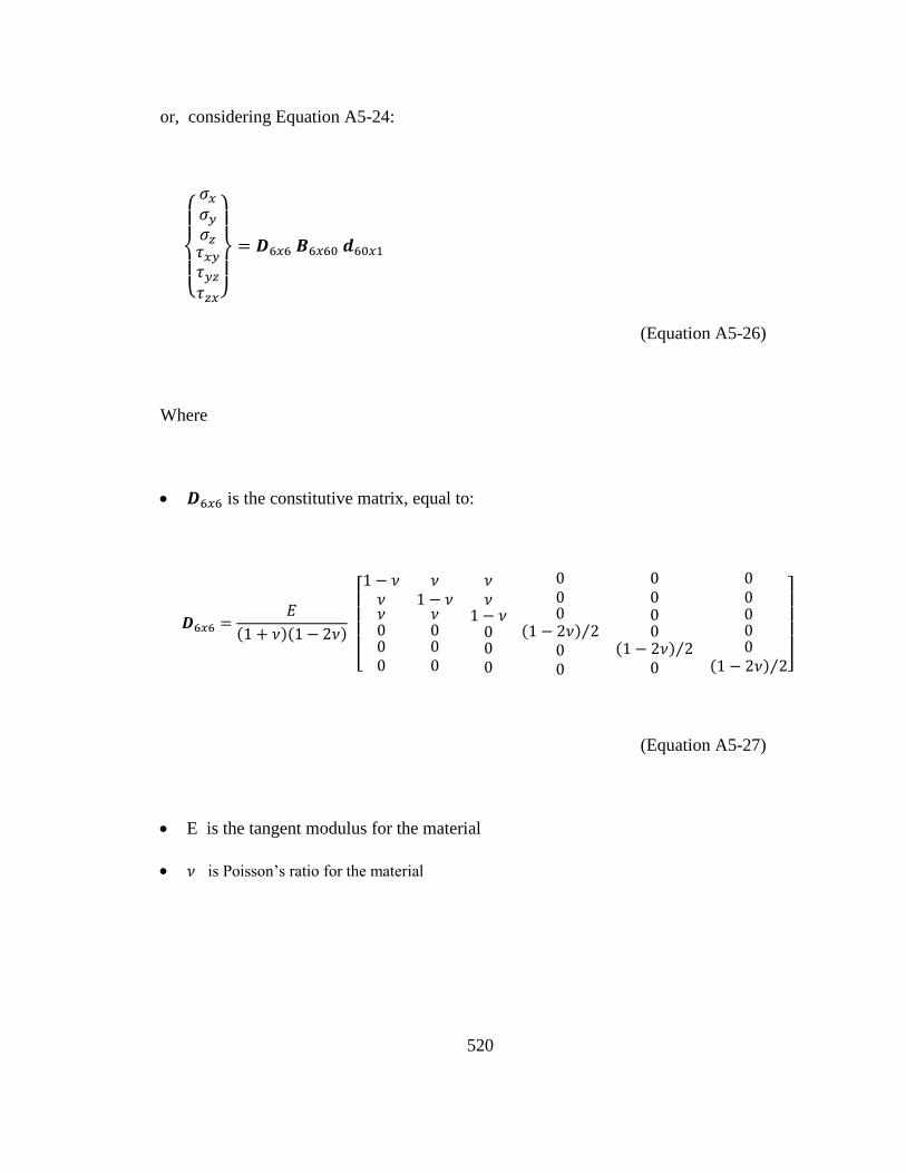
520
or, considering Equation A5-24:
{
}
(Equation A5-26)
Where
is the constitutive matrix, equal to:
( )( )
[
( ) ⁄
( ) ⁄
( ) ⁄ ]
(Equation A5-27)
E is the tangent modulus for the material
is Poisson’s ratio for the material

521
Step 4: Derive the Element Equilibrium Equations
The element equilibrium equations are derived using the principle of minimum potential
energy, as discussed in Logan (2007). It is noted that all of the terms in the derivation
reference the global coordinate system (x, y, z). The total potential energy can be
expressed as:
(Equation A5-28)
Where
denotes the strain energy, calculated as:
∭
(Equation A5-29)
and are the strain and stress vectors, respectively.
is the control volume.
denotes the potential energy of the body forces, calculated as:
∭
(Equation A5-30)
is the general displacement function in global coordinates, equal to:

522
{
( )
( ) ( )
}
(Equation A5-31)
is the weight density matrix, equal to:
{
}
(Equation A5-32)
, and denote the weight density in the x, y, and z-directions,
respectively.
denotes the potential energy of the concentrated loads, calculated as:
(Equation A5-33)
and are the nodal displacement and nodal load vectors,
respectively.
denotes the potential energy of the distributed loads (or surface tractions),
calculated as:
∬
(Equation A5-34)

523
is the vector of field of surface displacements through which the
distributed loads (or surface tractions) act.
is a vector containing the distributed loads (or surface tractions).
denotes the surface over which the distributed loads (or surface
tractions) act.
Considering the strain-displacement and stress-strain relations in global coordinates
(similar to Equations A5-23 and A5-25 expect that the strain-displacement matrix
is in terms of the global coordinates (x, y, z)), the total potential relation in Equation
A5-28 can be restructured as:
∭
∭
∬
(Equation A5-35)
Where
{
( ) ( ) ( )
}
(Equation A5-36)
{
( ) ( ) ( )
}
(Equation A5-37)

524
Considering that the nodal displacements are independent of the general coordinates,
Equation A5-35 becomes:
∭
∭
∬
(Equation A5-38)
The functional is then minimized with respect to the nodal displacement vector ,
as shown in Equation A5-39:
[∭
]
[∭
∬
]
(Equation A5-39)
Equation A5-39 can be restructured as:
(Equation A5-40)

525
Where
is the element stiffness matrix, equal to:
∭
(Equation A5-41)
is the nodal displacement vector
is the body force vector, equal to:
∭
(Equation A5-42)
is the nodal load vector, equal to:
(Equation A5-43)
is the distributed load (or surface traction) vector, equal to:
∬
(Equation A5-44)
Equations A5-41 through A5-44 present the element stiffness matrix and force vectors as
formulated in global coordinates (x, y, z). For the isoparametric formulation, however,
the matrices and are functions of the natural coordinates (s, t, z’). In order

526
to transform the variables and region from global (x, y, z) to natural (s, t, z’) coordinates,
the following theorem is utilized:
∬ ( )
∭ ( )| |
∭ ( )
∭ ( )| |
(Equations A5-45a-b)
Where
[
]
[
]
The mathematical proof for the theorem is provided in Thomas and Finney (1984).

527
Using the relations in Equations A5-45a-b, the element stiffness matrix and force vectors
are determined for the isoparametric formulation as follows:
∫ ∫ ∫ | |
(Equation A5-46)
∫ ∫ ∫
| |
(Equation A5-47)
(Equation A5-48)
∬
| |
(Equation A5-49)
where S is defined in terms of the natural coordinate system.
Integration of the terms in Equations A5-46, A5-47, and A5-49 is accomplished using a
numerical procedure, as illustrated in Equation A5-50 for the stiffness matrix:

528
∫ ∫ ∫ | |
∑ ( )
( ) | ( )|
(Equation A5-50)
Where
are weight factors used for the numerical integration scheme. The
reader is referred to Logan ( 2007) and Cheney and Kincaid (2008)
for additional details regarding numerical integration.
Step 5: Assemble the Global Equilibrium Equations and Introduce Boundary
Conditions
The global stiffness matrix is formulated using the direct stiffness method of assemblage,
considering transformation of element properties from the element local coordinate
system to the global coordinate system:
∑
(Equation A5-51)
Where
denotes the global stiffness matrix.
denotes the ith
element stiffness matrix.
denotes the number of elements in the global system.

529
The global load vector is formulated using a similar approach, which also considers
transformation from element local to global coordinates:
∑
(Equation A5-52)
Where
denotes the global load vector.
denotes the ith
element load vector.
denotes the number of element load vectors in the global system.
The global system of equations then takes the form:
(Equation A5-53)
Boundary conditions are applied by assigning kinematic nodal restraints and
body/nodal/element loads.
Step 6: Solve for the Nodal Displacements
Static condensation is generally used to extract the equations involving non-restrained
DOF, and a numerical procedure, e.g. Gaussian elimination, is utilized to solve the
homogeneous system of equations for the unknown nodal displacements. For the case of
imposed nodal displacements, however, the system of equations is nonhomogeneous, and
a numerical procedure referred to as the penalty method is commonly employed.
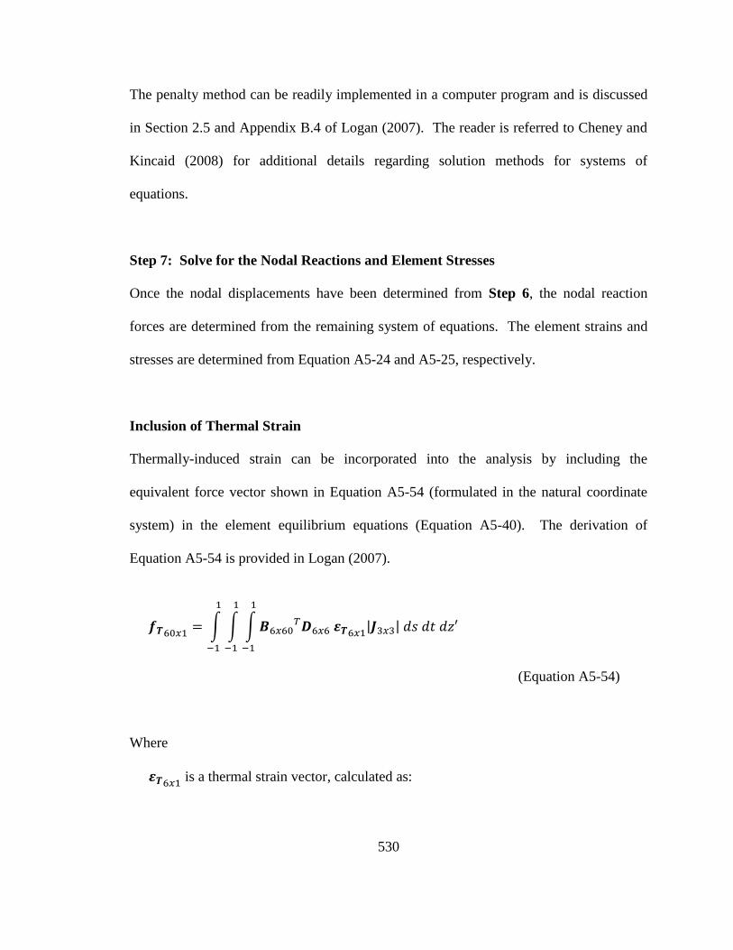
530
The penalty method can be readily implemented in a computer program and is discussed
in Section 2.5 and Appendix B.4 of Logan (2007). The reader is referred to Cheney and
Kincaid (2008) for additional details regarding solution methods for systems of
equations.
Step 7: Solve for the Nodal Reactions and Element Stresses
Once the nodal displacements have been determined from Step 6, the nodal reaction
forces are determined from the remaining system of equations. The element strains and
stresses are determined from Equation A5-24 and A5-25, respectively.
Inclusion of Thermal Strain
Thermally-induced strain can be incorporated into the analysis by including the
equivalent force vector shown in Equation A5-54 (formulated in the natural coordinate
system) in the element equilibrium equations (Equation A5-40). The derivation of
Equation A5-54 is provided in Logan (2007).
∫ ∫ ∫
| |
(Equation A5-54)
Where
is a thermal strain vector, calculated as:

531
{
}
(Equation A5-55)
For the case of isotropic materials, no temperature-induced shear strains will develop in
the material, i.e. the material will only be subject to thermal expansion or contraction. In
this scenario, the thermal strain vector can be expressed as:
{
}
{
}
(Equation A5-56)
Where
is the coefficient of thermal expansion for the material
is the temperature change relative to the baseline value
The element equilibrium equation considering thermal strain is then becomes:
(Equation A5-57)

532
Figure A5.1 20-node quadratic hexahedral continuum finite element:
global (x, y, z) and natural, or intrinsic, coordinates (s, t, z’)
(from Logan (2007))

533
VITA
Wesley John Keller was born in Pittsburgh, PA on December 24, 1979 to Richard and
Pamela Keller. He married Rebecca Kent Chance in September 2011.
He received a B.S. in Physics-Engineering from Washington and Lee University in 2002
and an M.S. in Civil Engineering from Virginia Tech University in 2004, and he is a
member of the Tau Beta Pi and Chi Epsilon national engineering societies and the Sigma
Xi national scientific research society.
He is a licensed Civil Engineer in the state of California and Professional Engineer in the
state of Pennsylvania. His professional experience was gained as a structural engineer at
Rummel, Klepper, and Kahl (RK&K), LLP in Baltimore, MD and as a structural/blast
engineer at Weidlinger Associates, Inc. in New York, NY.
In August 2007, he entered Lehigh University in pursuit of a Ph.D. in Structural
Engineering. He was awarded the Glenn J. Gibson Fellowship for the 2009-2010
academic term.
From August 2009 to December 2010, he participated in a collaborative venture between
researchers associated with the Network for Earthquake Engineering Simulation (NEES)
in the U.S. and the National Research Institute for Earth Science and Disaster Prevention

534
(NIED) in Japan. Under the guidance of Dr. Richard Sause, Director of Lehigh
University’s Center for Advanced Technology for Large Structural Systems (ATLSS), he
developed design details for an archetype self-centering post-tensioned concrete building
system and produced numerical response predictions for an experimental shake-table test
program. In December 2010, he was a National Science Foundation-sponsored visiting
research scientist at the Hyogo Earthquake Engineering Research Center (E-Defense) in
Hyogo, Japan.