Basic Principles of Ultrasonic Testing

Ultrasonic Testing (UT) uses high frequency sound energy to conduct examinations and make measurements. Ultrasonic inspectioncan be used for flaw detection/evaluation, dimensional measurements, material characterization, and more. To illustrate the general inspection principle, a typical pulse/echo inspectionconfiguration as illustrated below will be used.

A typical UT inspection system consists of several functional units, such as the pulser/receiver, transducer, and display devices. A pulser/receiver is an electronic device that can produce high voltage electrical pulses. Driven by the pulser, thetransducer generates high frequency ultrasonic energy. The sound energy is introduced and propagates through the materials in the form of waves. When there is a discontinuity (such as a crack) inthe wave path, part of the energy will be reflected back from theflaw surface. The reflected wave signal is transformed into an electrical signal by the transducer and is displayed on a screen.In the applet below, the reflected signal strength is displayed versus the time from signal generation to when a echo was received. Signal travel time can be directly related to the distance that the signal traveled. From the signal, information about the reflector location, size, orientation and other features can sometimes be gained.

Ultrasonic Inspection is a very useful and versatile NDT method. Some of the advantages of ultrasonic inspection that are often cited include:

It is sensitive to both surface and subsurface discontinuities.

The depth of penetration for flaw detection or measurement is superior to other NDT methods.

Only single-sided access is needed when the pulse-echo technique is used.

It is highly accurate in determining reflector position and estimating size and shape.

Minimal part preparation is required. Electronic equipment provides instantaneous results. Detailed images can be produced with automated systems. It has other uses, such as thickness measurement, in

addition to flaw detection.

As with all NDT methods, ultrasonic inspection also has its

limitations, which include:

Surface must be accessible to transmit ultrasound. Skill and training is more extensive than with some other

methods. It normally requires a coupling medium to promote the

transfer of sound energy into the test specimen. Materials that are rough, irregular in shape, very small,

exceptionally thin or not homogeneous are difficult to inspect.

Cast iron and other coarse grained materials are difficult to inspect due to low sound transmission and high signal noise.

Linear defects oriented parallel to the sound beam may go undetected.

Reference standards are required for both equipment calibration and the characterization of flaws.

The above introduction provides a simplified introduction to the NDT method of ultrasonic testing.  However, to effectively perform an inspection using ultrasonics, much more about the method needs to be known. The following pages present informationon the science involved in ultrasonic inspection, the equipment that is commonly used, some of the measurement techniques used, as well as other information.

History of Ultrasonics

Prior to World War II, sonar, the technique of sending sound waves through water and observing the returning echoes to characterize submerged objects, inspired early ultrasound investigators to explore ways to apply the concept to medical diagnosis. In 1929 and 1935, Sokolov studied the use of ultrasonic waves in detecting metal objects. Mulhauser, in 1931, obtained a patent for using ultrasonic waves, using two transducers to detect flaws in solids. Firestone (1940) and

Simons (1945) developed pulsed ultrasonic testing using a pulse-echo technique.

Shortly after the close of World War II, researchers in Japan began to explore the medical diagnostic capabilities of ultrasound. The first ultrasonic instruments used an A-mode presentation with blips on an oscilloscope screen. That was followed by a B-mode presentation with a two dimensional, gray scale image.

Japan's work in ultrasound was relatively unknown in the United States and Europe until the 1950s. Researchers then presented their findings on the use of ultrasound to detect gallstones, breast masses, and tumors to the international medical community.Japan was also the first country to apply Doppler ultrasound, an application of ultrasound that detects internal moving objects such as blood coursing through the heart for cardiovascular investigation.

Ultrasound pioneers working in the United States contributed manyinnovations and important discoveries to the field during the following decades. Researchers learned to use ultrasound to detect potential cancer and to visualize tumors in living subjects and in excised tissue. Real-time imaging, another significant diagnostic tool for physicians, presented ultrasound images directly on the system's CRT screen at the time of scanning. The introduction of spectral Doppler and later color Doppler depicted blood flow in various colors to indicate the speed and direction of the flow..

The United States also produced the earliest hand held "contact" scanner for clinical use, the second generation of B-mode equipment, and the prototype for the first articulated-arm hand held scanner, with 2-D images.

Beginnings of Nondestructive Evaluation (NDE)

Nondestructive testing has been practiced for many decades, with initial rapid developments in instrumentation spurred by the technological advances that occurred during World War II and the

subsequent defense effort. During the earlier days, the primary purpose was the detection of defects. As a part of "safe life" design, it was intended that a structure should not develop macroscopic defects during its life, with the detection of such defects being a cause for removal of the component from service. In response to this need, increasingly sophisticated techniques using ultrasonics, eddy currents, x-rays, dye penetrants, magnetic particles, and other forms of interrogating energy emerged.

In the early 1970's, two events occurred which caused a major change in the NDT field. First, improvements in the technology led to the ability to detect small flaws, which caused more partsto be rejected even though the probability of component failure had not changed. However, the discipline of fracture mechanics emerged, which enabled one to predict whether a crack of a given size will fail under a particular load when a material's fracturetoughness properties are known. Other laws were developed to predict the growth rate of cracks under cyclic loading (fatigue).With the advent of these tools, it became possible to accept structures containing defects if the sizes of those defects were known. This formed the basis for the new philosophy of  "damage tolerant" design. Components having known defects could continue in service as long as it could be established that those defects would not grow to a critical, failure producing size.

A new challenge was thus presented to the nondestructive testing community. Detection was not enough. One needed to also obtain quantitative information about flaw size to serve as an input to fracture mechanics based predictions of remaining life. The need for quantitative information was particularly strongly in the defense and nuclear power industries and led to the emergence of quantitative nondestructive evaluation (QNDE) as a new engineering/research discipline. A number of research programs around the world were started, such as the Center for Nondestructive Evaluation at Iowa State University (growing out of a major research effort at the Rockwell International Science Center); the Electric Power Research Institute in Charlotte, North Carolina; the Fraunhofer Institute for Nondestructive

Testing in Saarbrucken, Germany; and the Nondestructive Testing Centre in Harwell, England.

Present State of Ultrasonics

Ultrasonic testing (UT) has been practiced for many decades. Initial rapid developments in instrumentation spurred by the technological advances from the 1950's continue today. Through the 1980's and continuing through the present, computers have provided technicians with smaller and more rugged instruments with greater capabilities.

Thickness gauging is an example application where instruments have been refined make data collection easier and better.  Built-in data logging capabilities allow thousands of measurements to be recorded and eliminate the need for a "scribe."  Some instruments have the capability to capture waveforms as well as thickness readings. The waveform option allows an operator to view or review the A-scan signal of thickness measurement long after the completion of an inspection. Also, some instruments arecapable of modifying the measurement based on the surface conditions of the material.  For example, the signal from a pitted or eroded inner surface of a pipe would be treated differently than a smooth surface. This has led to more accurate and repeatable field measurements.

Many ultrasonic flaw detectors have a trigonometric function thatallows for fast and accurate location determination of flaws whenperforming shear wave inspections. Cathode ray tubes, for the most part, have been replaced with LED or LCD screens. These screens, in most cases, are extremely easy to view in a wide range of ambient lighting.  Bright or low light working conditions encountered by technicians have little effect on the technician's ability to view the screen. Screens can be adjusted for brightness, contrast, and on some instruments even the color of the screen and signal can be selected. Transducers can be programmed with predetermined instrument settings. The operator only has to connect the transducer and the instrument will set variables such as frequency and probe drive.

Along with computers, motion control and robotics have contributed to the advancement of ultrasonic inspections. Early on, the advantage of a stationary platform was recognized and used in industry. Computers can be programmed to inspect large, complex shaped components, with one or multiple transducers collecting information.  Automated systems typically consisted ofan immersion tank, scanning system, and recording system for a printout of the scan. The immersion tank can be replaced with a squirter systems, which allows the sound to be transmitted through a water column.  The resultant C-scan provides a plan or top view of the component. Scanning of components is considerablyfaster than contact hand scanning, the coupling is much more consistent.  The scan information is collected by a computer for evaluation, transmission to a customer, and archiving.

Today, quantitative theories have been developed to describe the interaction of the interrogating fields with flaws. Models incorporating the results have been integrated with solid model descriptions of real-part geometries to simulate practical inspections. Related tools allow NDE to be considered during the design process on an equal footing with other failure-related engineering disciplines. Quantitative descriptions of NDE performance, such as the probability of detection (POD), have become an integral part of statistical risk assessment. Measurement procedures initially developed for metals have been extended to engineered materials such as composites, where anisotropy and inhomogeneity have become important issues. The rapid advances in digitization and computing capabilities have totally changed the faces of many instruments and the type of algorithms that are used in processing the resulting data. High-resolution imaging systems and multiple measurement modalities for characterizing a flaw have emerged. Interest is increasing not only in detecting, characterizing, and sizing defects, but also in characterizing the materials. Goals range from the determination of fundamental microstructural characteristics suchas grain size, porosity, and texture (preferred grain orientation), to material properties related to such failure mechanisms as fatigue, creep, and fracture toughness. As technology continues to advance, applications of ultrasound also

advance. The high-resolution imaging systems in the laboratory today will be tools of the technician tomorrow.

Future Direction of Ultrasonic Inspection

Looking to the future, those in the field of NDE see an exciting new set of opportunities. The defense and nuclear power industries have played a major role in the emergence of NDE. Increasing global competition has led to dramatic changes in product development and business cycles. At the same time, aging infrastructure, from roads to buildings and aircraft, present a new set of measurement and monitoring challenges for engineers aswell as technicians.

Among the new applications of NDE spawned by these changes is theincreased emphasis on the use of NDE to improve the productivity of manufacturing processes. Quantitative nondestructive evaluation (QNDE) both increases the amount of information about failure modes and the speed with which information can be obtained and facilitates the development of in-line measurements for process control.

The phrase, "you cannot inspect in quality, you must build it in," exemplifies the industry's focus on avoiding the formation of flaws. Nevertheless, manufacturing flaws will never be completely eliminated and material damage will continue to occur in-service so continual development of flaw detection and characterization techniques is necessary.

Advanced simulation tools that are designed for inspectability and their integration into quantitative strategies for life management will contribute to increase the number and types of engineering applications of NDE. With growth in engineering applications for NDE, there will be a need to expand the knowledge base of technicians performing the evaluations. Advanced simulation tools used in the design for inspectability may be used to provide technical students with a greater understanding of sound behavior in materials. UTSIM, developed atIowa State University, provides a glimpse into what may be used in the technical classroom as an interactive laboratory tool.

As globalization continues, companies will seek to develop, with ever increasing frequency, uniform international practices. In the area of NDE, this trend will drive the emphasis on standards,enhanced educational offerings, and simulations that can be communicated electronically.  The coming years will be exciting as NDE will continue to emerge as a full-fledged engineering discipline.

Physics of Ultrasound

Wave Propagation

Ultrasonic testing is based on time-varying deformations or vibrations in materials, which is generally referred to as acoustics. All material substances are comprised of atoms, which may be forced into vibrational motion about their equilibrium positions. Many different patterns of vibrational motion exist atthe atomic level, however, most are irrelevant to acoustics and ultrasonic testing. Acoustics is focused on particles that contain many atoms that move in unison to produce a mechanical wave. When a material is not stressed in tension or compression beyond its elastic limit, its individual particles perform elastic oscillations. When the particles of a medium are displaced from their equilibrium positions, internal (electrostatic) restoration forces arise. It is these elastic restoring forces between particles, combined with inertia of the particles, that leads to the oscillatory motions of the medium.

In solids, sound waves can propagate in four principle modes thatare based on the way the particles oscillate. Sound can propagateas longitudinal waves, shear waves, surface waves, and in thin materials as plate waves. Longitudinal and shear waves are the two modes of propagation most widely used in ultrasonic testing. The particle movement responsible for the propagation of longitudinal and shear waves is illustrated below.

In longitudinal waves, theoscillations occur in the longitudinaldirection or the direction of wavepropagation. Since compressional anddilational forces are active in thesewaves, they are also called pressureor compressional waves. They are alsosometimes called density waves becausetheir particle density fluctuates asthey move. Compression waves can begenerated in liquids, as well as solids because the energy travels through the atomic structure by a series of compressions and expansion (rarefaction) movements.

 

In the transverse or shear wave, theparticles oscillate at a right angleor transverse to the direction ofpropagation. Shear waves require anacoustically solid material foreffective propagation, and therefore,are not effectively propagated inmaterials such as liquids or gasses.Shear waves are relatively weak whencompared to longitudinal waves. In

fact, shear waves are usually generated in materials using some of the energy from longitudinal waves.

 

Modes of Sound Wave Propagation

In air, sound travels by the compression and rarefaction of air molecules in the direction of travel.  However, in solids, molecules can support vibrations in other directions, hence, a number of different types of sound waves are possible.  Waves canbe characterized in space by oscillatory patterns that are capable of maintaining their shape and propagating in a stable manner.  The propagation of waves is often described in terms of what are called “wave modes.”

As mentioned previously, longitudinal and transverse (shear) waves are most often used in ultrasonic inspection.  However, at surfaces and interfaces, various types of elliptical or complex vibrations of the particles make other waves possible.  Some of these wave modes such as Rayleigh and Lamb waves are also useful for ultrasonic inspection.

The table below summarizes many, but not all, of the wave modes possible in solids.

Wave Types in Solids Particle VibrationsLongitudinal Parallel to wave directionTransverse (Shear) Perpendicular to wave directionSurface - Rayleigh Elliptical orbit - symmetrical mode Plate Wave - Lamb Component perpendicular to surface

(extensional wave) Plate Wave - Love Parallel to plane layer, perpendicular

to wave directionStoneley (Leaky Rayleigh Waves)

Wave guided along interface

Sezawa Antisymmetric mode

Longitudinal and transverse waves were discussed on the previous page, so let's touch on surface and plate waves here.

Surface (or Rayleigh) waves travel the surface of a relatively thick solid material penetrating to a depth of one wavelength. Surface waves combine both a longitudinal and transverse motion to create an elliptic orbit motion as shown in the image and animation below. The major axis of the ellipse is perpendicular to the surface of the solid. As the depth of an individual atom from the surface increases the width of its elliptical motion decreases. Surface waves are generated when a longitudinal wave intersects a surface near the second critical angle and they travel at a velocity between .87 and .95 of a shear wave.   Rayleigh waves are useful because they are very sensitive to surface defects (and other surface features) and they follow the surface around curves. Because of this, Rayleigh waves can be used to inspect areas that other waves might have difficulty reaching.

Plate waves are similar to surface waves except they can only be generated in materials a few wavelengths thick.  Lamb waves are the most commonly used plate waves in NDT.  Lamb waves are complex vibrational waves that propagate parallel to the test surface throughout the thickness of the material. Propagation of Lamb waves depends on the density and the elastic material properties of a component.  They are also influenced a great dealby the test frequency and material thickness. Lamb waves are generated at an incident angle in which the parallel component ofthe velocity of the wave in the source is equal to the velocity

of the wave in the test material. Lamb waves will travel several meters in steel and so are useful to scan plate, wire, and tubes.

With Lamb waves, a number of modes of particle vibration are possible, but the two most common are symmetrical and asymmetrical. The complex motion of the particles is similar to the elliptical orbits for surface waves.  Symmetrical Lamb waves move in a symmetrical fashion about the median plane of the plate.  This is sometimes called the extensional mode because thewave is “stretching and compressing” the plate in the wave motiondirection.  Wave motion in the symmetrical mode is most efficiently produced when the exciting force is parallel to the plate. The asymmetrical Lamb wave mode is often called the “flexural mode” because a large portion of the motion moves in a normal direction to the plate, and a little motion occurs in the direction parallel to the plate. In this mode, the body of the plate bends as the two surfaces move in the same direction.

The generation of waves using both piezoelectric transducers and electromagnetic acoustic transducers (EMATs) are discussed in later sections.

Properties of Acoustic Plane Wave

Wavelength, Frequency and Velocity

Among the properties of waves propagating in isotropic solid materials are wavelength, frequency, and velocity. The wavelengthis directly proportional to the velocity of the wave and inversely proportional to the frequency of the wave. This relationship is shown by the following equation.

The applet below shows a longitudinal and transverse wave. The direction of wave propagation is from left to right and the

movement of the lines indicate the direction of particle oscillation. The equation relating ultrasonic wavelength, frequency, and propagation velocity is included at the bottom of the applet in a reorganized form. The values for the wavelength, frequency, and wave velocity can be adjusted in the dialog boxes to see their effects on the wave. Note that the frequency value must be kept between 0.1 to 1 MHz (one million cycles per second)and the wave velocity must be between 0.1 and 0.7 cm/us.

As can be noted by the equation, a change in frequency will result in a change in wavelength. Change the frequency in the applet and view the resultant wavelength. At a frequency of .2 and a material velocity of 0.585 (longitudinal wave in steel) note the resulting wavelength. Adjust the material velocity to 0.480 (longitudinal wave in cast iron) and note the resulting wavelength. Increase the frequency to 0.8 and note the shortened wavelength in each material.

In ultrasonic testing, the shorter wavelength resulting from an increase in frequency will usually provide for the detection of smaller discontinuities. This will be discussed more in followingsections.

Wavelength and Defect Detection

In ultrasonic testing, the inspector must make a decision about the frequency of the transducer that will be used. As we learned on the previous page, changing the frequency when the sound

velocity is fixed will result in a change in the wavelength of the sound. The wavelength of the ultrasound used has a significant effect on the probability of detecting a discontinuity. A general rule of thumb is that a discontinuity must be larger than one-half the wavelength to stand a reasonablechance of being detected.

Sensitivity and resolution are two terms that are often used in ultrasonic inspection to describe a technique's ability to locateflaws. Sensitivity is the ability to locate small discontinuities. Sensitivity generally increases with higher frequency (shorter wavelengths). Resolution is the ability of thesystem to locate discontinuities that are close together within the material or located near the part surface. Resolution also generally increases as the frequency increases.

The wave frequency can also affect the capability of an inspection in adverse ways. Therefore, selecting the optimal inspection frequency often involves maintaining a balance betweenthe favorable and unfavorable results of the selection. Before selecting an inspection frequency, the material's grain structureand thickness, and the discontinuity's type, size, and probable location should be considered. As frequency increases, sound tends to scatter from large or course grain structure and from small imperfections within a material. Cast materials often have coarse grains and other sound scatters that require lower frequencies to be used for evaluations of these products. Wroughtand forged products with directional and refined grain structure can usually be inspected with higher frequency transducers.

Since more things in a material are likely to scatter a portion of the sound energy at higher frequencies, the penetrating power (or the maximum depth in a material that flaws can be located) isalso reduced. Frequency also has an effect on the shape of the ultrasonic beam. Beam spread, or the divergence of the beam from the center axis of the transducer, and how it is affected by frequency will be discussed later.

It should be mentioned, so as not to be misleading, that a numberof other variables will also affect the ability of ultrasound to

locate defects. These include the pulse length, type and voltage applied to the crystal, properties of the crystal, backing material, transducer diameter, and the receiver circuitry of the instrument. These are discussed in more detail in the material onsignal-to-noise ratio.

Sound Propagation in Elastic Materials

In the previous pages, it was pointed out that sound waves propagate due to the vibrations or oscillatory motions of particles within a material. An ultrasonic wave may be visualizedas an infinite number of oscillating masses or particles connected by means of elastic springs. Each individual particle is influenced by the motion of its nearest neighbor and both inertial and elastic restoring forces act upon each particle.

A mass on a spring has a single resonant frequency determined by its spring constant k and its mass m. The spring constant is the restoring force of a spring per unit of length. Within the elastic limit of any material, there is a linear relationship between the displacement of a particle and the force attempting to restore the particle to its equilibrium position. This linear dependency is described by Hooke's Law.

In terms of the spring model, Hooke's Law says that the restoringforce due to a spring is proportional to the length that the spring is stretched, and acts in the opposite direction. Mathematically, Hooke's Law is written as F =-kx, where F is the force, k is the spring constant, and x is the amount of particle displacement. Hooke's law is represented graphically it the right. Please note that the spring is applying a force to the particle that is equal and opposite to the force pulling down on the particle.

The Speed of Sound

Hooke's Law, when used along with Newton's Second Law, can explain a few things about the speed of sound. The speed of soundwithin a material is a function of the properties of the materialand is independent of the amplitude of the sound wave. Newton's

Second Law says that the force applied to a particle will be balanced by the particle's mass and the acceleration of the the particle. Mathematically, Newton's Second Law is written as F = ma. Hooke's Law then says that this force will be balanced by a force in the opposite direction that is dependent on the amount of displacement and the spring constant (F = -kx). Therefore, since the applied force and the restoring force are equal, ma = -kx can be written. The negative sign indicates that the force is in the opposite direction.

Since the mass m and the spring constant k are constants for any given material, it can be seen that the acceleration a and the displacement x are the only variables. It can also be seen that they are directly proportional. For instance, if the displacementof the particle increases, so does its acceleration. It turns outthat the time that it takes a particle to move and return to its equilibrium position is independent of the force applied. So, within a given material, sound always travels at the same speed no matter how much force is applied when other variables, such astemperature, are held constant.

What properties of material affect its speed of sound?

Of course, sound does travel at different speeds in different materials. This is because the mass of the atomic particles and the spring constants are different for different materials. The mass of the particles is related to the density of the material, and the spring constant is related to the elastic constants of a material. The general relationship between the speed of sound in a solid and its density and elastic constants is given by the following equation:

Where V is the speed of sound, C is the elastic constant, and p is the material density. This equation may take a number of

different forms depending on the type of wave (longitudinal or shear) and which of the elastic constants that are used. The typical elastic constants of a materials include:

Young's Modulus, E: a proportionality constant between uniaxial stress and strain.

Poisson's Ratio, n: the ratio of radial strain to axial strain

Bulk modulus, K: a measure of the incompressibility of a body subjected to hydrostatic pressure.

Shear Modulus, G: also called rigidity, a measure of a substance's resistance to shear.

Lame's Constants, l and m: material constants that are derived from Young's Modulus and Poisson's Ratio.

When calculating the velocity of a longitudinal wave, Young's Modulus and Poisson's Ratio are commonly used. When calculating the velocity of a shear wave, the shear modulus is used. It is often most convenient to make the calculations using Lame's Constants, which are derived from Young's Modulus and Poisson's Ratio.

It must also be mentioned that the subscript ij attached to C in the above equation is used to indicate the directionality of the elastic constants with respect to the wave type and direction of wave travel. In isotropic materials, the elastic constants are the same for all directions within the material. However, most materials are anisotropic and the elastic constants differ with each direction. For example, in a piece of rolled aluminum plate,the grains are elongated in one direction and compressed in the others and the elastic constants for the longitudinal direction are different than those for the transverse or short transverse directions.

Examples of approximate compressional sound velocities in materials are:

Aluminum - 0.632 cm/microsecond 1020 steel - 0.589 cm/microsecond Cast iron - 0.480 cm/microsecond.

Examples of approximate shear sound velocities in materials are:

Aluminum - 0.313 cm/microsecond 1020 steel - 0.324 cm/microsecond Cast iron - 0.240 cm/microsecond.

When comparing compressional and shear velocities, it can be noted that shear velocity is approximately one half that of compressional velocity. The sound velocities for a variety of materials can be found in the ultrasonic properties tables in thegeneral resources section of this site.

Attenuation of Sound Waves

When sound travels through a medium, its intensity diminishes with distance. In idealized materials, sound pressure (signal amplitude) is only reduced by the spreading of the wave. Natural materials, however, all produce an effect which further weakens the sound. This further weakening results from scattering and absorption. Scattering is the reflection of the sound in directions other than its original direction of propagation.  Absorption is the conversion of the sound energy to other forms of energy.  The combined effect of scattering and absorption is called attenuation.  Ultrasonic attenuation is the decay rate of the wave as it propagates through material.

Attenuation of sound within a material itself is often not of intrinsic interest. However, natural properties and loading conditions can be related to attenuation. Attenuation often serves as a measurement tool that leads to the formation of theories to explain physical or chemical phenomenon that decreases the ultrasonic intensity.

The amplitude change of a decaying plane wave can be expressed as:

In this expression A0 is the unattenuated amplitude of the propagating wave at some location. The amplitude A is the reduced amplitude after the wave has traveled a distance z from that initial location. The quantity is the attenuation coefficient of the wave traveling in the z-direction. The dimensions of are nepers/length, where a neper is a dimensionless quantity. The term e is the exponential (or Napier's constant) which is equal to approximately 2.71828.

The units of the attenuation value in Nepers per meter (Np/m) canbe converted to decibels/length by dividing by 0.1151. Decibels is a more common unit when relating the amplitudes of two signals.

Attenuation is generally proportional to the square of sound frequency. Quoted values of attenuation are often given for a single frequency, or an attenuation value averaged over many frequencies may be given. Also, the actual value of the attenuation coefficient for a given material is highly dependent on the way in which the material was manufactured. Thus, quoted values of attenuation only give a rough indication of the attenuation and should not be automatically trusted. Generally, areliable value of attenuation can only be obtained by determiningthe attenuation experimentally for the particular material being used.

Attenuation can be determined by evaluating the multiple backwallreflections seen in a typical A-scan display like the one shown in the image at the top of the page. The number of decibels between two adjacent signals is measured and this value is divided by the time interval between them. This calculation produces a attenuation coefficient in decibels per unit time Ut. This value can be converted to nepers/length by the following equation.

Where v is the velocity of sound in meters per second and Ut is in decibels per second.

Acoustic Impedance

Sound travels through materials under the influence of sound pressure. Because molecules or atoms of a solid are bound elastically to one another, the excess pressure results in a wavepropagating through the solid.

The acoustic impedance (Z) of a material is defined as the product of its density (p) and acoustic velocity (V).

Z = pV

Acoustic impedance is important in

1. the determination of acoustic transmission and reflection atthe boundary of two materials having different acoustic impedances.

2. the design of ultrasonic transducers.3. assessing absorption of sound in a medium.

The following applet can be used to calculate the acoustic impedance for any material, so long as its density (p) and acoustic velocity (V) are known.  The applet also shows how a change in the impedance affects the amount of acoustic energy that is reflected and transmitted.  The values of the reflected and transmitted energy are the fractional amounts of the total energy incident on the interface.  Note that the fractional amount of transmitted sound energy plus the fractional amount of reflected sound energy equals one.  The calculation used to arrive at these values will be discussed on the next page. 

 

eflection and Transmission Coefficients (Pressure)

Ultrasonic waves are reflected at boundaries where there is a difference in acoustic impedances (Z) of the materials on each side of the boundary. (See preceding page for more information onacoustic impedance.)  This difference in Z is commonly referred to as the impedance mismatch.  The greater the impedance mismatch, the greater the percentage of energy that will be reflected at the interface or boundary between one medium and another.

The fraction of the incident wave intensity that is reflected canbe derived because particle velocity and local particle pressuresmust be continuous across the boundary.  When the acoustic impedances of the materials on both sides of the boundary are known, the fraction of the incident wave intensity that is reflected can be calculated with the equation below.  The value produced is known as the reflection coefficient.  Multiplying thereflection coefficient by 100 yields the amount of energy reflected as a percentage of the original energy. 

Since the amount of reflected energy plus the transmitted energy must equal the total amount of incident energy, the transmission

coefficient is calculated by simply subtracting the reflection coefficient from one. 

Formulations for acoustic reflection and transmission coefficients (pressure) are shown in the interactive applet below.  Different materials may be selected or the material velocity and density may be altered to change the acoustic impedance of one or both materials. The red arrow represents reflected sound and the blue arrow represents transmitted sound.

Note that the reflection and transmission coefficients are often expressed in decibels (dB) to allow for large changes in signal strength to be more easily compared.  To convert the intensity orpower of the wave to dB units, take the log of the reflection or transmission coefficient and multiply this value times 10.  However, 20 is the multiplier used in the applet since the power of sound is not measured directly in ultrasonic testing.  The transducers produce a voltage that is approximately proportionally to the sound pressure.  The power carried by a traveling wave is proportional to the square of the pressure amplitude. Therefore, to estimate the signal amplitude change, the log of the reflection or transmission coefficient is multiplied by 20. 

Using the above applet, note that the energy reflected at a water-stainless steel interface is 0.88 or 88%. The amount of energy transmitted into the second material is 0.12 or 12%.  The

amount of reflection and transmission energy in dB terms are -1.1dB and -18.2 dB respectively.  The negative sign indicates that individually, the amount of reflected and transmitted energy is smaller than the incident energy.

If reflection and transmission at interfaces is followed through the component, only a small percentage of the original energy makes it back to the transducer, even when loss by attenuation isignored.  For example, consider an immersion inspection of a steel block.  The sound energy leaves the transducer, travels through the water, encounters the front surface of the steel, encounters the back surface of the steel and reflects back through the front surface on its way back to the transducer.  At the water steel interface (front surface), 12% of the energy is transmitted.  At the back surface, 88% of the 12% that made it through the front surface is reflected.  This is 10.6% of the intensity of the initial incident wave.  As the wave exits the part back through the front surface, only 12% of 10.6 or 1.3% of the original energy is transmitted back to the transducer.

 

Refraction and Snell's Law

When an ultrasonic wave passes through an interface between two materials at an oblique angle, and the materials have different indices of refraction, both reflected and refracted waves are produced. This also occurs with light, which is why objects seen across an interface appear to be shifted relative to where they really are. For example, if you look straight down at an object at the bottom of a glass of water, it looks closer than it reallyis. A good way to visualize how light and sound refract is to shine a flashlight into a bowl of slightly cloudy water noting the refraction angle with respect to the incident angle.

Refraction takes place at an interface due to the different velocities of the acoustic waves within the two materials. The velocity of sound in each material is determined by the material properties (elastic modulus and density) for that material. In the animation below, a series of plane waves are shown traveling in one material and entering a second material that has a higher acoustic velocity. Therefore, when the wave encounters the interface between these two materials, the portion of the wave inthe second material is moving faster than the portion of the wavein the first material. It can be seen that this causes the wave to bend.

Snell's Law describes the relationship between the angles and thevelocities of the waves. Snell's law equates the ratio of material velocities V1 and V2 to the ratio of the sine's of incident () and refracted () angles, as shown in the following equation.

Where:

VL1 is the longitudinal wave velocity in material 1.

VL2 is the longitudinal wave velocity in material 2.

 

Note that in the diagram, there is a reflected longitudinal wave (VL1' ) shown. This wave is reflected at the same angle as the incident wave because the two waves are traveling in the same material, and hence have the same velocities. This reflected waveis unimportant in our explanation of Snell's Law, but it should be remembered that some of the wave energy is reflected at the interface. In the applet below, only the incident and refracted

longitudinal waves are shown. The angle of either wave can be adjusted by clicking and dragging the mouse in the region of the arrows. Values for the angles or acoustic velocities can also be entered in the dialog boxes so the that applet can be used as a Snell's Law calculator.

When a longitudinal wave moves from a slower to a faster material, there is an incident angle that makes the angle of refraction for the wave 90o. This is know as the first critical angle. The first critical angle can be found from Snell's law by putting in an angle of 90° for the angle of the refracted ray. Atthe critical angle of incidence, much of the acoustic energy is in the form of an inhomogeneous compression wave, which travels along the interface and decays exponentially with depth from the interface. This wave is sometimes referred to as a "creep wave." Because of their inhomogeneous nature and the fact that they decay rapidly, creep waves are not used as extensively as Rayleigh surface waves in NDT. However, creep waves are sometimesmore useful than Rayleigh waves because they suffer less from surface irregularities and coarse material microstructure due to their longer wavelengths.

Mode Conversion

When sound travels in a solid material, one form of wave energy can be transformed into another form. For example, when a longitudinal waves hits an interface at an angle, some of the

energy can cause particle movement in the transverse direction tostart a shear (transverse) wave. Mode conversion occurs when a wave encounters an interface between materials of different acoustic impedances and the incident angle is not normal to the interface. From the ray tracing movie below, it can be seen that since mode conversion occurs every time a wave encounters an interface at an angle, ultrasonic signals can become confusing attimes.

In the previous section, it was pointed out that when sound wavespass through an interface between materials having different acoustic velocities, refraction takes place at the interface. Thelarger the difference in acoustic velocities between the two materials, the more the sound is refracted. Notice that the shearwave is not refracted as much as the longitudinal wave. This occurs because shear waves travel slower than longitudinal waves.Therefore, the velocity difference between the incident longitudinal wave and the shear wave is not as great as it is between the incident and refracted longitudinal waves. Also note

that when a longitudinal wave is reflected inside the material, the reflected shear wave is reflected at a smaller angle than thereflected longitudinal wave. This is also due to the fact that the shear velocity is less than the longitudinal velocity within a given material.

Snell's Law holds true for shear waves as well as longitudinal waves and can be written as follows.

Where:   VL1 is the longitudinal wave velocity in material 1.   VL2 is the longitudinal wave velocity in material 2.   VS1 is the shear wave velocity in material 1.   VS2 is the shear wave velocity in material 2.

In the applet below, the shear (transverse) wave ray path has been added. The ray paths of the waves can be adjusted by clicking and dragging in the vicinity of the arrows. Values for the angles or the wave velocities can also be entered into the dialog boxes. It can be seen from the applet that when a wave moves from a slower to a faster material, there is an incident angle which makes the angle of refraction for the longitudinal wave 90 degrees. As mentioned on the previous page, this is knownas the first critical angle and all of the energy from the refracted longitudinal wave is now converted to a surface following longitudinal wave. This surface following wave is sometime referred to as a creep wave and it is not very useful inNDT because it dampens out very rapidly.

Beyond the first critical angle, only the shear wave propagates into the material. For this reason, most angle beam transducers use a shear wave so that the signal is not complicated by having two waves present. In many cases there is also an incident angle that makes the angle of refraction for the shear wave 90 degrees.This is known as the second critical angle and at this point, allof the wave energy is reflected or refracted into a surface

following shear wave or shear creep wave. Slightly beyond the second critical angle, surface waves will be generated.

Note that the applet defaults to compressional velocity in the second material. The refracted compressional wave angle will be generated for given materials and angles. To find the angle of incidence required to generate a shear wave at a given angle complete the following:

1. Set V1 to the longitudinal wave velocity of material 1.  This material could be the transducer wedge or the immersionliquid.

2. Set V2 to the shear wave velocity (approximately one-half its compressional velocity) of the material to be inspected.

3. Set Q2 to the desired shear wave angle.4. Read Q1, the correct angle of incidence.

Signal-to-Noise Ratio

In a previous page, the effect that frequency and wavelength haveon flaw detectability was discussed. However, the detection of a defect involves many factors other than the relationship of wavelength and flaw size. For example, the amount of sound that reflects from a defect is also dependent on the acoustic impedance mismatch between the flaw and the surrounding material.A void is generally a better reflector than a metallic inclusion because the impedance mismatch is greater between air and metal than between two metals.

Often, the surrounding material has competing reflections. Microstructure grains in metals and the aggregate of concrete area couple of examples. A good measure of detectability of a flaw is its signal-to-noise ratio (S/N). The signal-to-noise ratio is a measure of how the signal from the defect compares to other background reflections (categorized as "noise"). A signal-to-noise ratio of 3 to 1 is often required as a minimum. The absolute noise level and the absolute strength of an echo from a "small" defect depends on a number of factors, which include:

The probe size and focal properties. The probe frequency, bandwidth and efficiency. The inspection path and distance (water and/or solid). The interface (surface curvature and roughness). The flaw location with respect to the incident beam. The inherent noisiness of the metal microstructure. The inherent reflectivity of the flaw, which is dependent on

its acoustic impedance, size, shape, and orientation. Cracks and volumetric defects can reflect ultrasonic waves

quite differently. Many cracks are "invisible" from one direction and strong reflectors from another.

Multifaceted flaws will tend to scatter sound away from the transducer.

The following formula relates some of the variables affecting thesignal-to-noise ratio (S/N) of a defect:

Rather than go into the details of this formulation, a few fundamental relationships can be pointed out. The signal-to-noiseratio (S/N), and therefore, the detectability of a defect:

Increases with increasing flaw size (scattering amplitude). The detectability of a defect is directly proportional to its size.

Increases with a more focused beam. In other words, flaw detectability is inversely proportional to the transducer beam width.

Increases with decreasing pulse width (delta-t). In other words, flaw detectability is inversely proportional to the duration of the pulse produced by an ultrasonic transducer. The shorter the pulse (often higher frequency), the better the detection of the defect. Shorter pulses correspond to broader bandwidth frequency response. See the figure below showing the waveform of a transducer and its corresponding frequency spectrum.

Decreases in materials with high density and/or a high ultrasonic velocity. The signal-to-noise ratio (S/N) is inversely proportional to material density and acoustic velocity.

Generally increases with frequency. However, in some materials, such as titanium alloys, both the "Aflaw" and the "Figure of Merit (FOM)" terms in the equation change at about the same rate with changing frequency. So, in some cases, the signal-to-noise ratio (S/N) can be somewhat independent of frequency.

Wave Interaction or Interference

Before we move into the next section, the subject of wave interaction must be covered since it is important when trying to understand the performance of an ultrasonic transducer. On the

previous pages, wave propagation was discussed as if a single sinusoidal wave was propagating through the material. However, the sound that emanates from an ultrasonic transducer does not originate from a single point, but instead originates from many points along the surface of the piezoelectric element. This results in a sound field with many waves interacting or interfering with each other.

When waves interact, they superimpose on each other, and the amplitude of the sound pressure or particle displacement at any point of interaction is the sum of the amplitudes of the two individual waves. First, let's consider two identical waves that originate from the same point. When they are in phase (so that thepeaks and valleys of one are exactly aligned with those of the other), they combine to double the displacement of either wave acting alone. When they are completely out of phase (so that the peaks of one wave are exactly aligned with the valleys of the other wave), they combine to cancel each other out. When the two waves are not completely in phase or out of phase, the resulting waveis the sum of the wave amplitudes for all points along the wave.

When the origins of the two interacting waves are not the same, it is a little harder to picture the wave interaction, but the principles are the same. Up until now, we have primarily looked at waves in the form of a 2D plot of wave amplitude versus wave position. However, anyone that has dropped something in a pool ofwater can picture the waves radiating out fromthe source with a circular wave front. If two objects are droppeda short distance apart into the pool of water, their waves will radiate out from their sources and interact with each other. At every point where the waves interact, the amplitude of the particle displacement is the combined sum of the amplitudes of the particle displacement of the individual waves.

With an ultrasonic transducer, the waves propagate out from the transducer face with a circular wave front. If it were possible to get the waves to propagate out from a single point on the transducer face, the sound field would appear as shown in the

upper image to the right. Consider the light areas to be areas ofrarefaction and the dark areas to be areas of compression.

However, as stated previously, sound waves originate from multiple points along the face of the transducer. The lower imageto the right shows what the sound field would look like if the waves originated from just two points. It can be seen that where the waves interact, there are areas of constructive and destructive interference. The points of constructive interferenceare often referred to as nodes. Of course, there are more than two points of origin along the face of a transducer. The image below shows five points of sound origination. It can be seen thatnear the face of the transducer, there are extensive fluctuationsor nodes and the sound field is very uneven. In ultrasonic testing, this in known as the near field (near zone) or Fresnel zone. The sound field is more uniform away from the transducer inthe far field, or Fraunhofer zone, where the beam spreads out in a pattern originating from the center of the transducer. It should be noted that even in the far field, it is not a uniform wave front. However, at some distance from the face of the transducer and central to the face of the transducer, a uniform and intense wave field develops.

Multiple points of sound origination along the face of the transducerStrong,uniform sound field

The curvature and the area over which the sound is being generated, the speed that the sound waves travel within a material and the frequency of the sound all affect the sound field. Use the Java applet below to experiment with these variables and see how the sound field is affected.

Equipment & Transducers

Piezoelectric Transducers

The conversion of electrical pulses to mechanical vibrations and the conversion of returned mechanical vibrations back into electrical energy is the basis for ultrasonic testing. The activeelement is the heart of the transducer as it converts the electrical energy to acoustic energy, and vice versa. The active element is basically a piece of polarized material (i.e. some parts of the molecule are positively charged, while other parts of the molecule are negatively charged) with electrodes attached to two of its opposite faces. When an electric field is applied across the material, the polarized molecules will align themselves with the electric field, resulting in induced dipoles

within the molecular or crystal structure of the material. This alignment of molecules will cause the material to change dimensions. This phenomenon is known as electrostriction. In addition, a permanently-polarized material such as quartz (SiO2) or barium titanate (BaTiO3) will produce an electric field when the material changes dimensions as a result of an imposed mechanical force. This phenomenon is known as the piezoelectric effect. Additional information on why certain materials produce this effect can be found in the linked presentation material, which was produced by the Valpey Fisher Corporation.

Piezoelectric Effect (PPT, 89kb)   Piezoelectric Elements (PPT, 178kb)

The active element of most acoustic transducers used today is a piezoelectric ceramic, which can be cut in various ways to produce different wave modes. A large piezoelectric ceramic element can be seen in the image of a sectioned low frequency transducer. Preceding the advent of piezoelectric ceramics in theearly 1950's, piezoelectric crystals made from quartz crystals and magnetostrictive materials were primarily used. The active element is still sometimes referred to as the crystal by old timers in the NDT field. When piezoelectric ceramics were introduced, they soon became the dominant material for transducers due to their good piezoelectric properties and their ease of manufacture into a variety of shapes and sizes. They alsooperate at low voltage and are usable up to about 300oC. The first piezoceramic in general use was barium titanate, and that was followed during the 1960's by lead zirconate titanate compositions, which are now the most commonly employed ceramic for making transducers. New materials such as piezo-polymers and composites are also being used in some applications.

The thickness of the active element is determined by the desired frequency of the transducer. A thin wafer element vibrates with awavelength that is twice its thickness. Therefore, piezoelectric crystals are cut to a thickness that is 1/2 the desired radiated wavelength. The higher the frequency of the transducer, the thinner the active element. The primary reason that high

frequency contact transducers are not produced is because the element is very thin and too fragile.

Characteristics of Piezoelectric Transducers

The transducer is a very important part of the ultrasonic instrumentation system. As discussed on the previous page, the transducer incorporates a piezoelectric element, which converts electrical signals into mechanical vibrations (transmit mode) andmechanical vibrations into electrical signals (receive mode). Many factors, including material, mechanical and electrical construction, and the external mechanical and electrical load conditions, influence the behavior of a transducer. Mechanical construction includes parameters such as the radiation surface area, mechanical damping, housing, connector type and other variables of physical construction. As of this writing, transducer manufacturers are hard pressed when constructing two transducers that have identical performance characteristics.

A cut away of a typical contact transducer is shown above. It waspreviously learned that the piezoelectric element is cut to 1/2 the desired wavelength. To get as much energy out of the transducer as possible, an impedance matching is placed between the active element and the face of the transducer. Optimal impedance matching is achieved by sizing the matching layer so that its thickness is 1/4 of the desired wavelength. This keeps

waves that were reflected within the matching layer in phase whenthey exit the layer (as illustrated in the image to the right). For contact transducers, the matching layer is made from a material that has an acoustical impedance between the active element and steel. Immersion transducers have a matching layer with an acoustical impedance between the active element and water. Contact transducers also incorporate a wear plate to protect the matching layer and active element from scratching.

The backing material supporting the crystal has a great influenceon the damping characteristics of a transducer. Using a backing material with an impedance similar to that of the active element will produce the most effective damping. Such a transducer will have a wider bandwidth resulting in higher sensitivity. As the mismatch in impedance between the active element and the backing material increases, material penetration increases but transducersensitivity is reduced.

Transducer Efficiency, Bandwidth and Frequency

Some transducers are specially fabricated to be more efficient transmitters and others to be more efficient receivers. A transducer that performs well in one application will not always produce the desired results in a different application. For example, sensitivity to small defects is proportional to the product of the efficiency of the transducer as a transmitter and a receiver. Resolution, the ability to locate defects near the surface or in close proximity in the material, requires a highly damped transducer.

It is also important to understand the concept of bandwidth, or range of frequencies, associated with a transducer. The frequencynoted on a transducer is the central or center frequency and depends primarily on the backing material. Highly damped transducers will respond to frequencies above and below the central frequency. The broad frequency range provides a transducer with high resolving power. Less damped transducers will exhibit a narrower frequency range and poorer resolving power, but greater penetration. The central frequency will also define the capabilities of a transducer. Lower frequencies

(0.5MHz-2.25MHz) provide greater energy and penetration in a material, while high frequency crystals (15.0MHz-25.0MHz) providereduced penetration but greater sensitivity to small discontinuities. High frequency transducers, when used with the proper instrumentation, can improve flaw resolution and thicknessmeasurement capabilities dramatically. Broadband transducers withfrequencies up to 150 MHz are commercially available.

Transducers are constructed to withstand some abuse, but they should be handled carefully. Misuse, such as dropping, can cause cracking of the wear plate, element, or the backing material. Damage to a transducer is often noted on the A-scan presentation as an enlargement of the initial pulse.

Radiated Fields of Ultrasonic Transducers

The sound that emanates from a piezoelectric transducer does not originate from a point, but instead originates from most of the surface of the piezoelectric element. Round transducers are oftenreferred to as piston source transducers because the sound field resembles a cylindrical mass in front of the transducer. The sound field from a typical piezoelectric transducer is shown below. The intensity of the sound is indicated by color, with lighter colors indicating higher intensity.

Since the ultrasound originates from a number of points along thetransducer face, the ultrasound intensity along the beam is affected by constructive and destructive wave interference as discussed in a previous page on wave interference. These are sometimes also referred to as diffraction effects. This wave interference leads to extensive fluctuations in the sound intensity near the source and is known as the near field. Becauseof acoustic variations within a near field, it can be extremely difficult to accurately evaluate flaws in materials when they arepositioned within this area.

The pressure waves combine to form a relatively uniform front at the end of the near field. The area beyond the near field where the ultrasonic beam is more uniform is called the far field. In the far field, the beam spreads out in a pattern originating fromthe center of the transducer. The transition between the near field and the far field occurs at a distance, N, and is sometimes referred to as the "natural focus" of a flat (or unfocused) transducer. The near/far field distance, N, is significant because amplitude variations that characterize the near field change to a smoothly declining amplitude at this point. The area just beyond the near field is where the sound wave is well behaved and at its maximum strength. Therefore, optimal detection results will be obtained when flaws occur in this area.

 

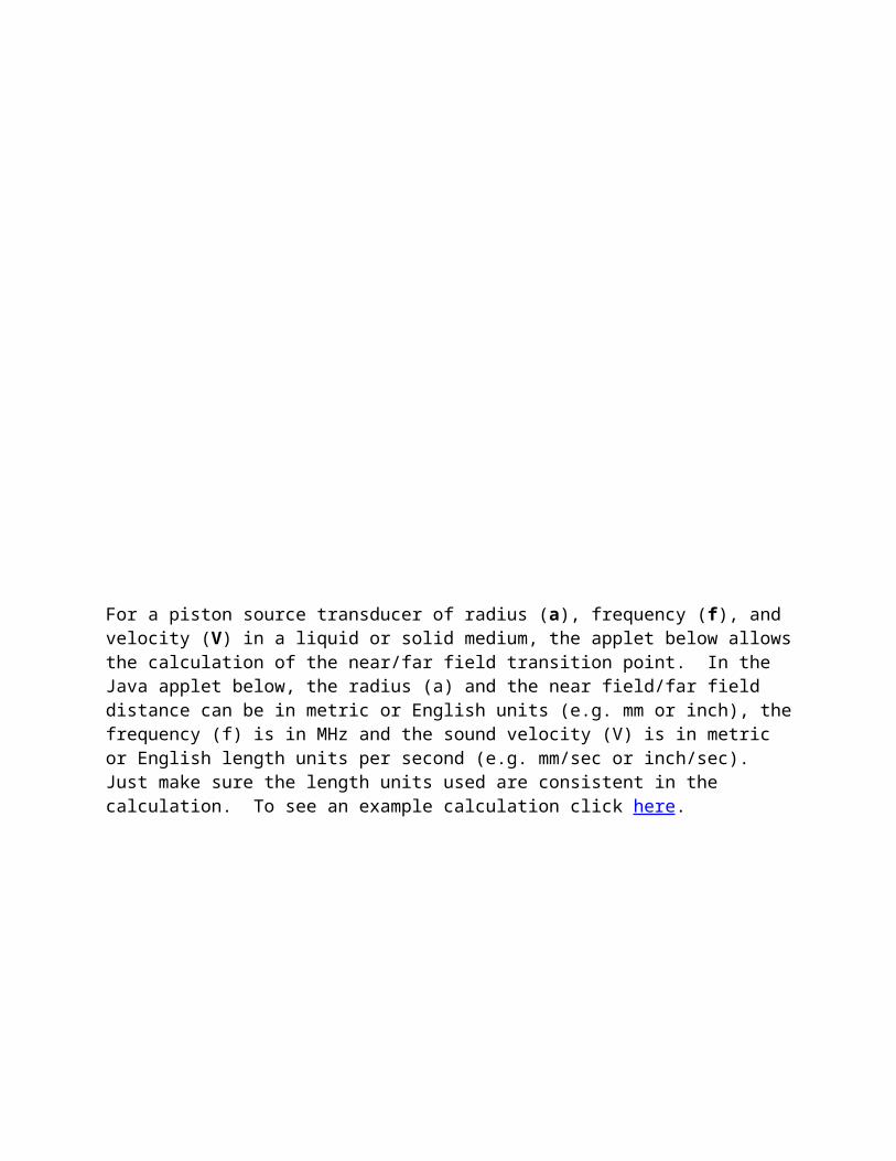
For a piston source transducer of radius (a), frequency (f), and velocity (V) in a liquid or solid medium, the applet below allowsthe calculation of the near/far field transition point.  In the Java applet below, the radius (a) and the near field/far field distance can be in metric or English units (e.g. mm or inch), thefrequency (f) is in MHz and the sound velocity (V) is in metric or English length units per second (e.g. mm/sec or inch/sec).  Just make sure the length units used are consistent in the calculation.  To see an example calculation click here. 

Spherical or cylindrical focusing changes the structure of a transducer field by "pulling" the N point nearer the transducer.It is also important to note that the driving excitation normallyused in NDT applications are either spike or rectangular pulsars,not a single frequency. This can significantly alter the performance of a transducer. Nonetheless, the supporting analysisis widely used because it represents a reasonable approximation and a good starting point.

Transducer Beam Spread

As discussed on the previous page, round transducers are often referred to as piston source transducers because the sound field resembles a cylindrical mass in front of the transducer. However,the energy in the beam does not remain in a cylinder, but insteadspreads out as it propagates through the material. The phenomenonis usually referred to as beam spread but is sometimes also referred to as beam divergence or ultrasonic diffraction. It should be noted that there is actually a difference between beam spread and beam divergence. Beam spread is a measure of the wholeangle from side to side of the main lobe of the sound beam in thefar field. Beam divergence is a measure of the angle from one side of the sound beam to the central axis of the beam in the farfield. Therefore, beam spread is twice the beam divergence.

Although beam spread must be considered when performing an ultrasonic inspection, it is important to note that in the far field, or Fraunhofer zone, the maximum sound pressure is always found along the acoustic axis (centerline) of the transducer. Therefore, the strongest reflections are likely to come from the area directly in front of the transducer.

Beam spread occurs because the vibrating particle of the material(through which the wave is traveling) do not always transfer all of their energy in the direction of wave propagation. Recall thatwaves propagate through the transfer of energy from one particle to another in the medium. If the particles are not directly aligned in the direction of wave propagation, some of the energy will get transferred off at an angle. (Picture what happens when one ball hits another ball slightly off center). In the near

field, constructive and destructive wave interference fill the sound field with fluctuation. At the start of the far field, however, the beam strength is always greatest at the center of the beam and diminishes as it spreads outward.

As shown in the applet below, beam spread is largely determined by the frequency and diameter of the transducer. Beam spread is greater when using a low frequency transducer than when using a high frequency transducer. As the diameter of the transducer increases, the beam spread will be reduced.

Beam angle is an important consideration in transducer selection for a couple of reasons. First, beam spread lowers the amplitude of reflections since sound fields are less concentrated and, thereby weaker. Second, beam spread may result in more difficultyin interpreting signals due to reflections from the lateral sidesof the test object or other features outside of the inspection area. Characterization of the sound field generated by a transducer is a prerequisite to understanding observed signals.

Numerous codes exist that can be used to standardize the method used for the characterization of beam spread. American Society for Testing and Materials ASTM E-1065, addresses methods for ascertaining beam shapes in Section A6, Measurement of Sound Field Parameters. However, these measurements are limited to immersion probes. In fact, the methods described in E-1065 are primarily concerned with the measurement of beam characteristics in water, and as such are limited to measurements of the compression mode only. Techniques described in E-1065 include pulse-echo using a ball target and hydrophone receiver, which allows the sound field of the probe to be assessed for the entirevolume in front of the probe.

For a flat piston source transducer, an approximation of the beamspread may be calculated as a function of the transducer diameter(D), frequency (F), and the sound velocity (V) in the liquid or solid medium. The applet below allows the beam divergence angle (1/2 the beam spread angle) to be calculated. This angle represents a measure from the center of the acoustic axis to the point where the sound pressure has decreased by one half (-6 dB) to the side of the acoustic axis in the far field.

Note: This applet uses the equation:

Where:

θ = Beam divergence angle from centerline to point where signal is at half strength.

  V = Sound velocity in the material. (inch/sec or cm/sec)1

  a = Radius of the transducer. (inch or cm)1   F = Frequency of the transducer. (cycles/second) Note 1: Units must be consistent throughout calculation (i.e. inch or cm but not both)

An equal, but perhaps more common version of the formula is:

Where:

θ = Beam divergence angle from centerline to point where signal is at half strength.

  V = Sound velocity in the material. (inch/sec or cm/sec)

  D = Diameter of the transducer. (inch or cm)  F = Frequency of the transducer. (cycles/second)

Transducer Types

Ultrasonic transducers are manufactured for a variety of applications and can be custom fabricated when necessary. Carefulattention must be paid to selecting the proper transducer for theapplication. A previous section on Acoustic Wavelength and DefectDetection gave a brief overview of factors that affect defect detectability. From this material, we know that it is important to choose transducers that have the desired frequency, bandwidth,and focusing to optimize inspection capability. Most often the transducer is chosen either to enhance the sensitivity or resolution of the system.

Transducers are classified into groups according to the application.

Contact transducers are used for direct contact inspections,and are generally hand manipulated. They have elements protected in a rugged casing to withstand sliding contact with a variety of materials. These transducers have an ergonomic design so that they are easy to grip and move along a surface. They often have replaceable wear plates to lengthen their useful life. Coupling materials of water, grease, oils, or commercial materials are used to remove theair gap between the transducer and the component being inspected.

Immersion transducers do not contact the component. These transducers are designed to operate in a liquid environment and all connections are watertight. Immersion transducers usually have an impedance matching layer that helps to get more sound energy into the water and, in turn, into the component being inspected. Immersion transducers can be purchased with a planer, cylindrically focused or spherically focused lens. A focused transducer can improve the sensitivity and axial resolution by concentrating the sound energy to a smaller area. Immersion transducers are typically used inside a water tank or as part of a squirter or bubbler system in scanning applications.

More on Contact Transducers.

Contact transducers are available in a variety of configurations to improve their usefulness for a variety of applications. The flat contact transducer shown above is used in normal beam inspections of relatively flat surfaces, and where near surface resolution is not critical. If the surface is curved, a shoe thatmatches the curvature of the part may need to be added to the face of the transducer. If near surface resolution is important or if an angle beam inspection is needed, one of the special contact transducers described below might be used.

Dual element transducers contain two independently operated elements in a single housing. One of the elements transmits and the other receives the ultrasonic signal. Active elements can be chosen for their sending and receiving capabilities to provide a transducer with a cleaner signal, and transducers for special

applications, such as the inspection of course grained material. Dual element transducers are especially well suited for making measurements in applications where reflectors are very near the transducer since this design eliminates the ring down effect thatsingle-element transducers experience (when single-element transducers are operating in pulse echo mode, the element cannot start receiving reflected signals until the element has stopped ringing from its transmit function). Dual element transducers arevery useful when making thickness measurements of thin materials and when inspecting for near surface defects. The two elements are angled towards each other to create a crossed-beam sound pathin the test material.

Delay line transducers provide versatility with a variety of replaceable options. Removable delay line, surface conforming membrane, and protective wear cap options can make a single transducer effective for a wide range of applications. As the name implies, the primary function of a delay line transducer is to introduce a time delay between the generation of the sound wave and the arrival of any reflected waves. This allows the transducer to complete its "sending" function before it starts its "listening" function so that near surface resolution is improved. They are designed for use in applications such as high precision thickness gauging of thin materials and delamination checks in composite materials. They are also useful in high-temperature measurement applications since the delay line provides some insulation to the piezoelectric element from the heat.

Angle beam transducers and wedges are typically used to introducea refracted shear wave into the test material. Transducers can bepurchased in a variety of fixed angles or in adjustable versions where the user determines the angles of incidence and refraction.In the fixed angle versions, the angle of refraction that is marked on the transducer is only accurate for a particular material, which is usually steel. The angled sound path allows the sound beam to be reflected from the backwall to improve detectability of flaws in and around welded areas. They are also

used to generate surface waves for use in detecting defects on the surface of a component.

Normal incidence shear wave transducers are unique because they allow the introduction of shear waves directly into a test piece without the use of an angle beam wedge. Careful design has enabled manufacturing of transducers with minimal longitudinal wave contamination. The ratio of the longitudinal to shear wave components is generally below -30dB.

Paint brush transducers are used to scan wide areas. These long and narrow transducers are made up of an array of small crystals that are carefully matched to minimize variations in performance and maintain uniform sensitivity over the entire area of the transducer. Paint brush transducers make it possible to scan a larger area more rapidly for discontinuities. Smaller and more sensitive transducers are often then required to further define the details of a discontinuity.

ransducer Testing

Some transducer manufacturers have lead in the development of transducer characterization techniques and have participated in developing the AIUM Standard Methods for Testing Single-Element Pulse-Echo Ultrasonic Transducers as well as ASTM-E 1065 StandardGuide for Evaluating Characteristics of Ultrasonic Search Units.

Additionally, some manufacturers perform characterizations according to AWS, ESI, and many other industrial and military standards. Often, equipment in test labs is maintained in compliance with MIL-C-45662A Calibration System Requirements. As part of the documentation process, an extensive database containing records of the waveform and spectrum of each transducer is maintained and can be accessed for comparative or statistical studies of transducer characteristics.

Manufacturers often provide time and frequency domain plots for each transducer. The signals below were generated by a spiked pulser. The waveform image on the left shows the test response signal in the time domain (amplitude versus time). The spectrum

image on the right shows the same signal in the frequency domain (amplitude versus frequency). The signal path is usually a reflection from the back wall (fused silica) with the reflection in the far field of the transducer.

Other tests may include the following:

Electrical Impedance Plots provide important information about the design and construction of a transducer and can allow users to obtain electrically similar transducers from multiple sources.

Beam Alignment Measurements provide data on the degree of alignment between the sound beam axis and the transducer housing. This information is particularly useful in applications that require a high degree of certainty regarding beam positioning with respect to a mechanical reference surface.

Beam Profiles provide valuable information about transducer sound field characteristics. Transverse beam profiles are created by scanning the transducer across a target (usually either a steel ball or rod) at a given distance from the transducer face and are used to determine focal spot size and beam symmetry. Axial beam profiles are created by recording the pulse-echo amplitude of the sound field as a function of distance from the transducer face and provide data on depth of field and focal length.

Transducer Testing II

As noted in the ASTM E1065 Standard Guide for Evaluating Characteristics of Ultrasonic Transducers, the acoustic and electrical characteristics which can be described from the data, are obtained from specific procedures that are listed below:

Frequency Response--The frequency response may be obtained from one of two procedures: shock excitation and sinusoidal burst.

Relative Pulse-Echo Sensitivity--The relative pulse-echo sensitivity may be obtained from the frequency response databy using a sinusoidal burst procedure. The value is obtainedfrom the relationship of the amplitude of the voltage applied to the transducer and the amplitude of the pulse-echo signal received from a specified target.

Time Response--The time response provides a means for describing the radio frequency (RF) response of the waveform. A shock excitation, pulse-echo procedure is used to obtain the response. The time or waveform responses are recorded from specific targets that are chosen for the type of transducer under evaluation, for example, immersion, contact straight beam, or contact angle beam.

Typical time and frequency domain plots providedby transducer manufacturers

Frequency Response--The frequency response of the above transducer has a peak at 5 MHz and operates over a broad range of frequencies. Its bandwidth (4.1 to 6.15 MHz) is measured at the -6 dB points, or 70% of the peak frequency. The useable bandwidth of broadband transducers, especially in frequency analysis measurements, is often quoted at the -20 dB points. Transducer sensitivity and bandwidth (more of

one means less of the other) are chosen based on inspection needs.

Complex Electrical Impedance--The complex electrical impedance may be obtained with commercial impedance measuring instrumentation, and these measurements may provide the magnitude and phase of the impedance of the search unit over the operating frequency range of the unit. These measurements are generally made under laboratory conditions with minimum cable lengths or external accessories and in accordance with specifications given by the instrument manufacturer. The value of the magnitude of the complex electrical impedance may also be obtained using values recorded from the sinusoidal burst.

Sound Field Measurements--The objective of these measurements is to establish parameters such as the on-axis and transverse sound beam profiles for immersion, and flat and curved transducers. These measurements are often achieved by scanning the sound field with a hydrophone transducer to map the sound field in three dimensional space. An alternative approach to sound field measurements is a measure of the transducer's radiating surface motion using laser interferometry.

Transducer Modeling In high-technology manufacturing, part design and simulation

of part inspection is done in the virtual world of the computer. Transducer modeling is necessary to make accurate predictions of how a part or component might be inspected, prior to the actual building of that part. Computer modelingis also used to design ultrasonic transducers.

As noted in the previous section, an ultrasonic transducer may be characterized by detailed measurements of its electrical and sound radiation properties. Such measurementscan completely determine the response of any one individual transducer.

There is ongoing research to develop general models that relate electrical inputs (voltage, current) to mechanical outputs (force, velocity) and vice-versa. These models can be very robust in giving accurate prediction of transducer response, but suffer from a lack of accurate modeling of

physical variables inherent in transducer manufacturing. These electrical-mechanical response models must take into account the physical and electrical components in the figurebelow.

The Thompson-Gray Measurement Model, which makes very accurate predictions of ultrasonic scattering measurements made through liquid-solid interfaces, does not attempt to model transducer electrical-mechanical response. The Thompson-Gray Measurement Model approach makes use of reference data taken with the same transducer(s) to deconvolve electro-physical characteristics specific to individual transducers. See Section 5.4 Thompson-Gray Measurement Model.

The long term goal in ultrasonic modeling is to incorporate accurate models of the transducers themselves as well as accurate models of pulser-receivers, cables, and other components that completely describe any given inspection setup and allow the accurate prediction of inspection signals.

Couplant A couplant is a material (usually liquid) that facilitates

the transmission of ultrasonic energy from the transducer into the test specimen. Couplant is generally necessary because the acoustic impedance mismatch between air and solids (i.e. such as the test specimen) is large. Therefore,

nearly all of the energy is reflected and very little is transmitted into the test material. The couplant displaces the air and makes it possible to get more sound energy into the test specimen so that a usable ultrasonic signal can be obtained. In contact ultrasonic testing a thin film of oil, glycerin or water is generally used between the transducer and the test surface.

When scanning over the part or making precise measurements, an immersion technique is often used. In immersion ultrasonic testing both the transducer and the part are immersed in the couplant, which is typically water. This method of coupling makes it easier to maintain consistent coupling while moving and manipulating the transducer and/orthe part.

  .

Electromagnetic Acoustic Transducers (EMATs)

As discussed on the previous page, one of the essential features of ultrasonic measurements is mechanical coupling between the transducer and the solid whose properties or structure are to be studied. This coupling is generally achieved in one of two ways. In immersion measurements, energy is coupled between the transducer and sample by placing both objects in a tank filled with a fluid, generally water. In contact measurements, the transducer is pressed directly against the sample, and coupling is achieved by the presence of a thin fluid layer inserted between the two. When shear waves are to be transmitted, the fluid is generally selected to have a significant viscosity.

Electromagnetic-acoustic transducers (EMAT) acts through totally different physical principles and do not need couplant. When a wire is placed near the surface of an electrically conducting object and is driven by a current at the desired ultrasonic frequency, eddy currents will be induced in a near surface regionof the object. If a static magnetic field is also present, these eddy currents will experience Lorentz forces of the form

F = J x B

F is the body force per unit volume, J is the induced dynamic current density, and B is the static magnetic induction.

The most important application of EMATs has been in nondestructive evaluation (NDE) applications such as flaw detection or material property characterization. Couplant free transduction allows operation without contact at elevated temperatures and in remote locations. The coil and magnet structure can also be designed to excite complex wave patterns and polarizations that would be difficult to realize with fluid coupled piezoelectric probes. In the inference of material properties from precise velocity or attenuation measurements, using EMATs can eliminate errors associated with couplant variation, particularly in contact measurements.

A number of practical EMAT configurations are shown below. In each, the biasing magnet structure, the coil, and the forces on the surface of the solid are shown in an exploded view. The firstthree configurations will excite beams propagating normal to the surface of the half-space and produce beams with radial, longitudinal, and transverse polarizations, respectively. The final two use spatially varying stresses to excite beams propagating at oblique angles or along the surface of a component. Although a great number of variations on these configurations have been conceived and used in practice, consideration of these three geometries should suffice to introduce the fundamentals.

Cross-sectional view of a spiral coil EMAT exciting radially

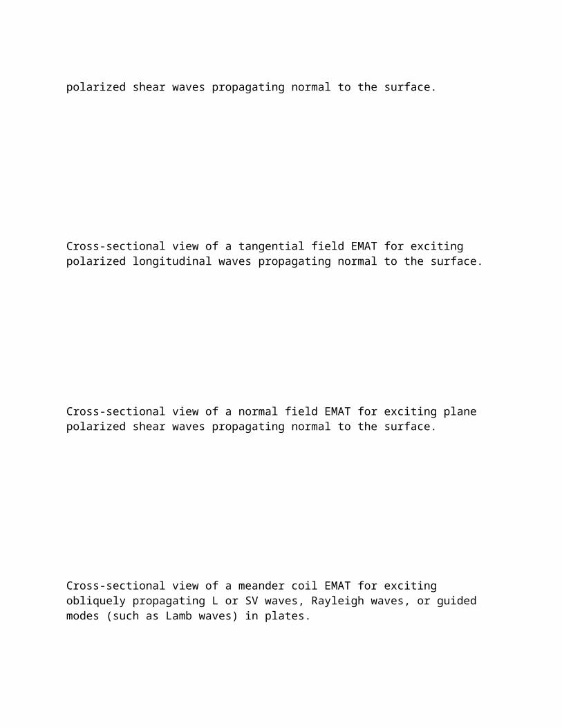
polarized shear waves propagating normal to the surface.

Cross-sectional view of a tangential field EMAT for exciting polarized longitudinal waves propagating normal to the surface.

Cross-sectional view of a normal field EMAT for exciting plane polarized shear waves propagating normal to the surface.

Cross-sectional view of a meander coil EMAT for exciting obliquely propagating L or SV waves, Rayleigh waves, or guided modes (such as Lamb waves) in plates.

Cross-sectional view of a periodic permanent magnet EMAT for exciting grazing or obliquely propagating horizontally polarized (SH) waves or guided SH modes in plates.

Practical EMAT designs are relatively narrowband and require strong magnetic fields and large currents to produce ultrasound that is often weaker than that produced by piezoelectric transducers. Rare-earth materials such as Samarium-Cobalt and Neodymium-Iron-Boron are often used to produce sufficiently strong magnetic fields, which may also be generated by pulsed electromagnets.

The EMAT offers many advantages based on its couplant-free operation. These advantages include the abilities to operate in remote environments at elevated speeds and temperatures, to excite polarizations not easily excited by fluid coupled piezoelectrics, and to produce highly consistent measurements.

These advantages are tempered by low efficiencies, and careful electronic design is essential to applications.

More information about the use of EMATs can be found at the following links.

Lamb Wave Generation With EMATsShear Wave Generation With EMATsVelocity Measurements With EMATsTexture Measurement I With EMATsTexture Measurement II With EMATsStress Measurement With EMATsComposite inspection With EMATs

Pulser-Receivers

Ultrasonic pulser-receivers are well suited to general purpose ultrasonic testing. Along with appropriate transducers and an oscilloscope, they can be used for flaw detection and thickness gauging in a wide variety of metals, plastics, ceramics, and composites. Ultrasonic pulser-receivers provide a unique, low-cost ultrasonic measurement capability.

The pulser section of the instrument generates short, large amplitude electric pulses of controlled energy, which are converted into short ultrasonic pulses when applied to an ultrasonic transducer. Most pulser sections have very low impedance outputs to better drive transducers. Control functions associated with the pulser circuit include:

Pulse length or damping (The amount of time the pulse is applied to the transducer.)

Pulse energy (The voltage applied to the transducer. Typicalpulser circuits will apply from 100 volts to 800 volts to a transducer.)

In the receiver section the voltage signals produced by the transducer, which represent the received ultrasonic pulses, are amplified. The amplified radio frequency (RF) signal is availableas an output for display or capture for signal processing. Control functions associated with the receiver circuit include

Signal rectification (The RF signal can be viewed as positive half wave, negative half wave or full wave.)

Filtering to shape and smooth return signals Gain, or signal amplification Reject control

The pulser-receiver is also used in material characterization work involving sound velocity or attenuation measurements, which can be correlated to material properties such as elastic modulus.  In conjunction with a stepless gate and a spectrum analyzer, pulser-receivers are also used to study frequency dependent material properties or to characterize the performance of ultrasonic transducers.

Tone Burst Generators In Research

Tone burst generators are often used in high power ultrasonic applications. They take low-voltage signals and convert them intohigh-power pulse trains for the most power-demanding applications. Their purpose is to transmit bursts of acoustic energy into a test piece, receive the resulting signals, and thenmanipulate and analyze the received signals in various ways. Highpower radio frequency (RF) burst capability allows researchers towork with difficult, highly attenuative materials or inefficient transducers such as EMATs. A computer interface makes it possiblefor systems to make high speed complex measurements, such as those involving multiple frequencies.

Arbitrary Function Generators

Arbitrary waveform generators permit the user to design and generate virtually any waveform in addition to the standard function generator signals (i.e. sine wave, square wave, etc.). Waveforms are generated digitally from a computer's memory, and most instruments allow the downloading of digital waveform files from computers.

Ultrasonic generation pulses must be varied to accommodate different types of ultrasonic transducers. General-purpose highlydamped contact transducers are usually excited by a wideband,

spike-like pulse provided by many common pulser/receiver units. The lightly damped transducers used in high power generation, forexample, require a narrowband tone-burst excitation from a separate generator unit. Sometimes the same transducer will be excited differently, such as in the study of the dispersion of a material's ultrasonic attenuation or to characterize ultrasonic transducers.

Section of biphase modulated spread spectrum ultrasonic waveform

In spread spectrum ultrasonics (see spread spectrum page), encoded sound is generated by an arbitrary waveform generator continuously transmitting coded sound into the part or structure being tested. Instead of receiving echoes, spread spectrum ultrasonics generates an acoustic correlation signature having a one-to-one correspondence with the acoustic state of the part or structure (in its environment) at the instant of measurement. In its simplest embodiment, the acoustic correlation signature is generated by cross correlating an encoding sequence (with suitable cross and auto correlation properties) transmitted into a part (structure) with received signals returning from the part (structure).

Electrical Impedance Matching and Termination

When computer systems were first introduced decades ago, they were large, slow-working devices that were incompatible with eachother. Today, national and international networking standards have established electronic control protocols that enable different systems to "talk" to each other. The Electronics Industries Associations (EIA) and the Institute of Electrical andElectronics Engineers (IEEE) developed standards that establishedcommon terminology and interface requirements, such as EIA RS-232and IEEE 802.3. If a system designer builds equipment to comply with these standards, the equipment will interface with other

systems. But what about analog signals that are used in ultrasonics?

Data Signals: Input versus Output

Consider the signal going to and from ultrasonic transducers. When you transmit data through a cable, the requirement usually simplifies into comparing what goes in one end with what comes out the other. High frequency pulses degrade or deteriorate when they are passed through any cable. Both the height of the pulse (magnitude) and the shape of the pulse (wave form) change dramatically, and the amount of change depends on the data rate, transmission distance and the cable's electrical characteristics.Sometimes a marginal electrical cable may perform adequately if used in only short lengths, but the same cable with the same datain long lengths will fail. This is why system designers and industry standards specify precise cable criteria.

Recommendation: Observe manufacturer's recommended practices for cable impedance, cable length, impedance matching, and any requirements for termination in characteristic impedance.

Recommendation: If possible, use the same cables and cable dressing for all inspections.

Cable Electrical Characteristics

The most important characteristics in an electronic cable are impedance, attenuation, shielding, and capacitance. In this page,we can only review these characteristics very generally, however,we will discuss capacitance in more detail.

Impedance (Ohms) represents the total resistance that the cable presents to the electrical current passing through it. At low frequencies the impedance is largely a function of the conductor size, but at high frequencies conductor size, insulation material, and insulation thickness all affect the cable's impedance. Matching impedance is very important. If the system isdesigned to be 100 Ohms, then the cable should match that impedance, otherwise error-producing reflections are created.

Attenuation is measured in decibels per unit length (dB/m), and provides an indication of the signal loss as it travels through the cable. Attenuation is very dependent on signal frequency. A cable that works very well with low frequency data may do very poorly at higher data rates. Cables with lower attenuation are better.

Shielding is normally specified as a cable construction detail. For example, the cable may be unshielded, contain shielded pairs,have an overall aluminum/mylar tape and drain wire, or have a double shield. Cable shields usually have two functions: to act as a barrier to keep external signals from getting in and internal signals from getting out, and to be a part of the electrical circuit. Shielding effectiveness is very complex to measure and depends on the data frequency within the cable and the precise shield design. A shield may be very effective in one frequency range, but a different frequency may require a completely different design. System designers often test completecable assemblies or connected systems for shielding effectiveness.

Capacitance in a cable is usually measured as picofarads per foot(pf/m). It indicates how much charge the cable can store within itself. If a voltage signal is being transmitted by a twisted pair, the insulation of the individual wires becomes charged by the voltage within the circuit. Since it takes a certain amount of time for the cable to reach its charged level, this slows downand interferes with the signal being transmitted. Digital data pulses are a string of voltage variations that are represented bysquare waves. A cable with a high capacitance slows down these signals so that they come out of the cable looking more like "saw-teeth," rather than square waves. The lower the capacitance of the cable, the better it performs with high speed data.

Data Presentation

Ultrasonic data can be collected and displayed in a number of different formats. The three most common formats are know in the NDT world as A-scan, B-scan and C-scan presentations. Each presentation mode provides a different way of looking at and

evaluating the region of material being inspected. Modern computerized ultrasonic scanning systems can display data in all three presentation forms simultaneously.

A-Scan Presentation

The A-scan presentation displays the amount of received ultrasonic energy as a function of time. The relative amount of received energy is plotted along the vertical axis and the elapsed time (which may be related to the sound energy travel time within the material) is displayed along the horizontal axis.Most instruments with an A-scan display allow the signal to be displayed in its natural radio frequency form (RF), as a fully rectified RF signal, or as either the positive or negative half of the RF signal. In the A-scan presentation, relative discontinuity size can be estimated by comparing the signal amplitude obtained from an unknown reflector to that from a knownreflector. Reflector depth can be determined by the position of the signal on the horizontal sweep.

In the illustration of the A-scan presentation to the right, the initial pulse generated by the transducer is represented by the signal IP, which is near time zero. As the transducer is scanned along the surface of the part, four other signals are likely to appear at different times on the screen. When the transducer is in its far left position, only the IP signal and signal A, the sound energy reflecting from surface A, will be seen on the trace. As the transducer is scanned to the right, a signal from the backwall BW will appear later in time, showing that the soundhas traveled farther to reach this surface. When the transducer is over flaw B, signal B will appear at a point on the time scale that is approximately halfway between the IP signal and theBW signal. Since the IP signal corresponds to the front surface of the material, this indicates that flaw B is about halfway between the front and back surfaces of the sample. When the transducer is moved over flaw C, signal C will appear earlier in time since the sound travel path is shorter and signal B will disappear since sound will no longer be reflecting from it.

B-Scan Presentation

The B-scan presentations is a profile (cross-sectional) view of the test specimen. In the B-scan, the time-of-flight (travel time) of the sound energy is displayed along the vertical axis and the linear position of the transducer is displayed along the horizontal axis. From the B-scan, the depth of the reflector and its approximate linear dimensions in the scan direction can be determined. The B-scan is typically produced by establishing a trigger gate on the A-scan. Whenever the signal intensity is great enough to trigger the gate, a point is produced on the B-scan. The gate is triggered by the sound reflecting from the backwall of the specimen and by smaller reflectors within the material. In the B-scan image above, line A is produced as the transducer is scanned over the reduced thickness portion of the specimen. When the transducer moves to the right of this section,the backwall line BW is produced. When the transducer is over flaws B and C, lines that are similar to the length of the flawsand at similar depths within the material are drawn on the B-scan. It should be noted that a limitation to this display technique is that reflectors may be masked by larger reflectors near the surface.

C-Scan Presentation

The C-scan presentation provides a plan-type view of the locationand size of test specimen features. The plane of the image is parallel to the scan pattern of the transducer. C-scan presentations are produced with an automated data acquisition system, such as a computer controlled immersion scanning system. Typically, a data collection gate is established on the A-scan and the amplitude or the time-of-flight of the signal is recordedat regular intervals as the transducer is scanned over the test piece. The relative signal amplitude or the time-of-flight is displayed as a shade of gray or a color for each of the positionswhere data was recorded. The C-scan presentation provides an image of the features that reflect and scatter the sound within and on the surfaces of the test piece.

High resolution scans can produce very detailed images. Below aretwo ultrasonic C-scan images of a US quarter. Both images were produced using a pulse-echo technique with the transducer scannedover the head side in an immersion scanning system. For the C-scan image on the left, the gate was setup to capture the amplitude of the sound reflecting from the front surface of the quarter. Light areas in the image indicate areas that reflected agreater amount of energy back to the transducer. In the C-scan image on the right, the gate was moved to record the intensity ofthe sound reflecting from the back surface of the coin. The details on the back surface are clearly visible but front surfacefeatures are also still visible since the sound energy is affected by these features as it travels through the front surface of the coin.

Error Analysis

All measurements, including ultrasonic measurements, however careful and scientific, are subject to some uncertainties. Error analysis is the study and evaluation of these uncertainties; its two main functions being to allow the practitioner to estimate how large the uncertainties are and to help him or her to reduce them when necessary. Because ultrasonics depends on measurements,evaluation and minimization of uncertainties is crucial.

In science the word "error" does not mean "mistake" or "blunder" but rather the inevitable uncertainty of all measurements. Because they cannot be avoided, errors in this context are not, strictly speaking, "mistakes." At best, they can be made as smallas reasonably possible, and their size can be reliably estimated.

To illustrate the inevitable occurrence of uncertainties surrounding attempts at measurement, let us consider a carpenter who must measure the height of a doorway to an X-ray vault in order to install a door. As a first rough measurement, she might simply look at the doorway and estimate that it is 210 cm high. This crude "measurement" is certainly subject to uncertainty. If pressed, the carpenter might express this uncertainty by admitting that the height could be as little as 205 or as much as

215 cm.

If she wanted a more accurate measurement, she would use a tape measure, and she might find that the height is 211.3 cm. This measurement is certainly more precise than her original estimate,but it is obviously still subject to some uncertainty, since it is inconceivable that she could know the height to be exactly 211.3000 rather than 211.3001 cm, for example.

There are many reasons for this remaining uncertainty. Some of these causes of uncertainty could be removed if enough care were taken. For example, one source of uncertainty might be that poor lighting is making it difficult to read the tape; this could be corrected by improved lighting.

On the other hand, some sources of uncertainty are intrinsic to the process of measurement and can never be entirely removed. Forinstance, let us suppose the carpenter's tape is graduated in half-centimeters. The top of the door will probably not coincide precisely with one of the half-centimeter marks, and if it does not, then the carpenter must estimate just where the top lies between two marks. Even if the top happens to coincide with one of the marks, the mark itself is perhaps a millimeter wide, so she must estimate just where the top lies within the mark. In either case, the carpenter ultimately must estimate where the topof the door lies relative to the markings on her tape, and this necessity causes some uncertainty in her answer.

By buying a better tape with closer and finer markings, the carpenter can reduce her uncertainty, but she cannot eliminate itentirely. If she becomes obsessively determined to find the height of the door with the greatest precision that is technically possible, she could buy an expensive laser interferometer. But even the precision of an interferometer is limited to distances on the order of the wavelength of light (about 0.000005 meters). Although she would now be able to measure the height with fantastic precision, she still would not know the height of the doorway exactly.

Furthermore, as the carpenter strives for greater precision, she will encounter an important problem of principle. She will certainly find that the height is different in different places. Even in one place, she will find that the height varies if the temperature and humidity vary, or even if she accidentally rubs off a thin layer of dirt. In other words, she will find that there is no such thing as one exact height of the doorway. This kind of problem is called a "problem of definition" (the height of the door is not well-defined and plays an important role in many scientific measurements).

Our carpenter's experiences illustrate what is found to be generally true. No physical quantity (a thickness, time between pulse-echoes, a transducer position, etc.) can be measured with complete certainty. With care we may be able to reduce the uncertainties until they are extremely small, but to eliminate them entirely is impossible.

In everyday measurements we do not usually bother to discuss uncertainties. Sometimes the uncertainties are simply not interesting. If we say that the distance between home and school is 3 miles, it does not matter (for most purposes) whether this means "somewhere between 2.5 and 3.5 miles" or "somewhere between2.99 and 3.01 miles." Often the uncertainties are important, but can be allowed for instinctively and without explicit consideration. When our carpenter comes to fit her door, she mustknow its height with an uncertainty that is less than 1 mm or so.However, as long as the uncertainty is this small, the door will (for all practical purposes) be a perfect fit, x-rays will not leak out, and her concern with error analysis will come to an end.

Normal Beam Inspection

Pulse-echo ultrasonic measurements can determine the location of a discontinuity in a part or structure by accurately measuring the time required for a short ultrasonic pulse generated by a transducer to travel through a thickness of material, reflect from the back or the surface of a discontinuity, and be returned

to the transducer. In most applications, this time interval is a few microseconds or less. The two-way transit time measured is divided by two to account for the down-and-back travel path and multiplied by the velocity of sound in the test material. The result is expressed in the well-known relationship

d = vt/2 or v = 2d/t

where d is the distance from the surface to the discontinuity in the test piece, v is the velocity of sound waves in the material,and t is the measured round-trip transit time.

The diagram below allows you to move a transducer over the surface of a stainless steel test block and see return echoes as they would appear on an oscilloscope. The transducer employed is a 5 MHz broadband transducer 0.25 inches in diameter. The signalswere generated with computer software similar to that found in the Thompson-Gray Measurement Model and UTSIM developed at the Center for Nondestructive Evaluation at Iowa State University.

Precision ultrasonic thickness gages usually operate at frequencies between 500 kHz and 100 MHz, by means of piezoelectric transducers that generate bursts of sound waves when excited by electrical pulses. A wide variety of transducers with various acoustic characteristics have been developed to meetthe needs of industrial applications. Typically, lower frequencies are used to optimize penetration when measuring thick, highly attenuating or highly scattering materials, while higher frequencies will be recommended to optimize resolution in thinner, non-attenuating, non-scattering materials.

In thickness gauging, ultrasonic techniques permit quick and reliable measurement of thickness without requiring access to

both sides of a part. Accuracy's as high as ±1 micron or ±0.0001 inch can be achieved in some applications. It is possible to measure most engineering materials ultrasonically, including metals, plastic, ceramics, composites, epoxies, and glass as wellas liquid levels and the thickness of certain biological specimens. On-line or in-process measurement of extruded plasticsor rolled metal often is possible, as is measurements of single layers or coatings in multilayer materials. Modern handheld gagesare simple to use and very reliable.

Angle Beams I

Angle Beam Transducers and wedges are typically used to introducea refracted shear wave into the test material. An angled sound path allows the sound beam to come in from the side, thereby improving detectability of flaws in and around welded areas.

Crack Tip Diffraction

When the geometry of the part is relatively uncomplicated and theorientation of a flaw is well known, the length (a) of a crack can be determined by a technique known as tip diffraction. One common application of the tip diffraction technique is to determine the length of a crack originating from on the backside of a flat plate as shown below. In this case, when an angle beam transducer is scanned over the area of the flaw, the principle echo comes from the base of the crack to locate the position of the flaw (Image 1). A second, much weaker echo comes from the tipof the crack and since the distance traveled by the ultrasound isless, the second signal appears earlier in time on the scope (Image 2).

 

Crack height (a) is a function of the ultrasound velocity (v) in the material, the incident angle and the difference in arrival times between the two signal (dt). Since the incident angle and the thickness of the material is the same in both measurements, two similar right triangle are formed such that onecan be overlayed on the other. A third similar right triangle is made, which is comprised on the crack, the length dt and the angleThe variable dt is really the difference in time but caneasily be converted to a distance by dividing the time in half (to get the one-way travel time) and multiplying this value by the velocity of the sound in the material. Using trigonometry an equation for estimating crack height from these variables can be derived as shown below.

Solving for "a" the equation becomes

The equation is complete once distance dt is calculated by dividing the difference in time between the two signals (dt) by two and multiplying this value by the sound velocity.

Automated Scanning

Ultrasonic scanning systems are used for automated data acquisition and imaging. They typically integrate a ultrasonic instrumentation, a scanning bridge, and computer controls. The signal strength and/or the time-of-flight of the signal is measured for every point in the scan plan. The value of the data is plotted using colors or shades of gray to produce detailed images of the surface or internal features of a component. Systems are usually capable of displaying the data in A-, B- and C-scan modes simultaneously. With any ultrasonic scanning system there are two factors to consider:

1. how to generate and receive the ultrasound.2. how to scan the transducer(s) with respect to the part being

inspected.

The most common ultrasonic scanning systems involve the use of animmersion tank as shown in the image above. The ultrasonic transducer and the part are placed under water so that consistentcoupling is maintained by the water path as the transducer or part is moved within the tank. However, scanning systems come in a large variety of configurations to meet specific inspection needs. In the image to the right, an engineer aligns the heads ofa squirter system that uses a through-transmission technique to inspect aircraft composite structures. In this system, the

ultrasound travels through columns of forced water which are scanned about the part with a robotic system. A variation of the squirter system is the "Dripless Bubbler" scanning system, which is discussed below.

It is often desirable to eliminate the need for the water coupling and a number of state-of-the-art UT scanning systems have done this. Laser ultrasonic systems use laser beams to generate the ultrasound and collect the resulting signals in an noncontact mode. Advances in transducer technology has lead to the development of an inspection technique known as air-coupled ultrasonic inspection. These systems are capable of sending ultrasonic energy through air and getting enough energy into the part to have a useable signal. These system typically use a through-transmission technique since reflected energy from discontinuities are too weak to detect.

The second major consideration is how toscan the transducer(s) with respect to thepart being inspected. When the sample beinginspected has a flat surface, a simpleraster-scan can be performed. If the sampleis cylindrical, a turntable can be used toturn the sample while the transducer is heldstationary or scanned in the axial directionof the cylinder. When the sample isirregular shaped, scanning becomes moredifficult. As illustrated in the beam modeling animation, curved surface can steer, focus and defocus the ultrasonic beam. For inspection applications involving parts having complex curvatures, scanning systems capable of performing contour following are usually necessary.

Precision Velocity Measurements

Changes in ultrasonic wave propagation speed, along with energy losses, from interactions with a materials microstructures are often used to nondestructively gain information about a material's properties. Measurements of sound velocity and ultrasonic wave attenuation can be related to the elastic

properties that can be used to characterize the texture of polycrystalline metals. These measurements enable industry to replace destructive microscopic inspections with nondestructive methods.

Of interest in velocity measurements are longitudinal wave, whichpropagate in gases, liquids, and solids. In solids, also of interest are transverse (shear) waves. The longitudinal velocity is independent of sample geometry when the dimensions at right angles to the beam are large compared to the beam area and wavelength. The transverse velocity is affected little by the physical dimensions of the sample.

Pulse-Echo and Pulse-Echo-Overlap Methods

Rough ultrasonic velocity measurements are as simple as measuringthe time it takes for a pulse of ultrasound to travel from one transducer to another (pitch-catch) or return to the same transducer (pulse-echo). Another method is to compare the phase of the detected sound wave with a reference signal: slight changes in the transducer separation are seen as slight phase changes, from which the sound velocity can be calculated. These methods are suitable for estimating acoustic velocity to about 1 part in 100. Standard practice for measuring velocity in materials is detailed in ASTM E494.

Precision Velocity Measurements (using EMATs)

Electromagnetic-acoustic transducers (EMAT) generate ultrasound in the material being investigated. When a wire or coil is placednear to the surface of an electrically conducting object and is driven by a current at the desired ultrasonic frequency, eddy currents will be induced in a near surface region. If a static magnetic field is also present, these currents will experience Lorentz forces of the form

F = J x B

where F is a body force per unit volume, J is the induced dynamic

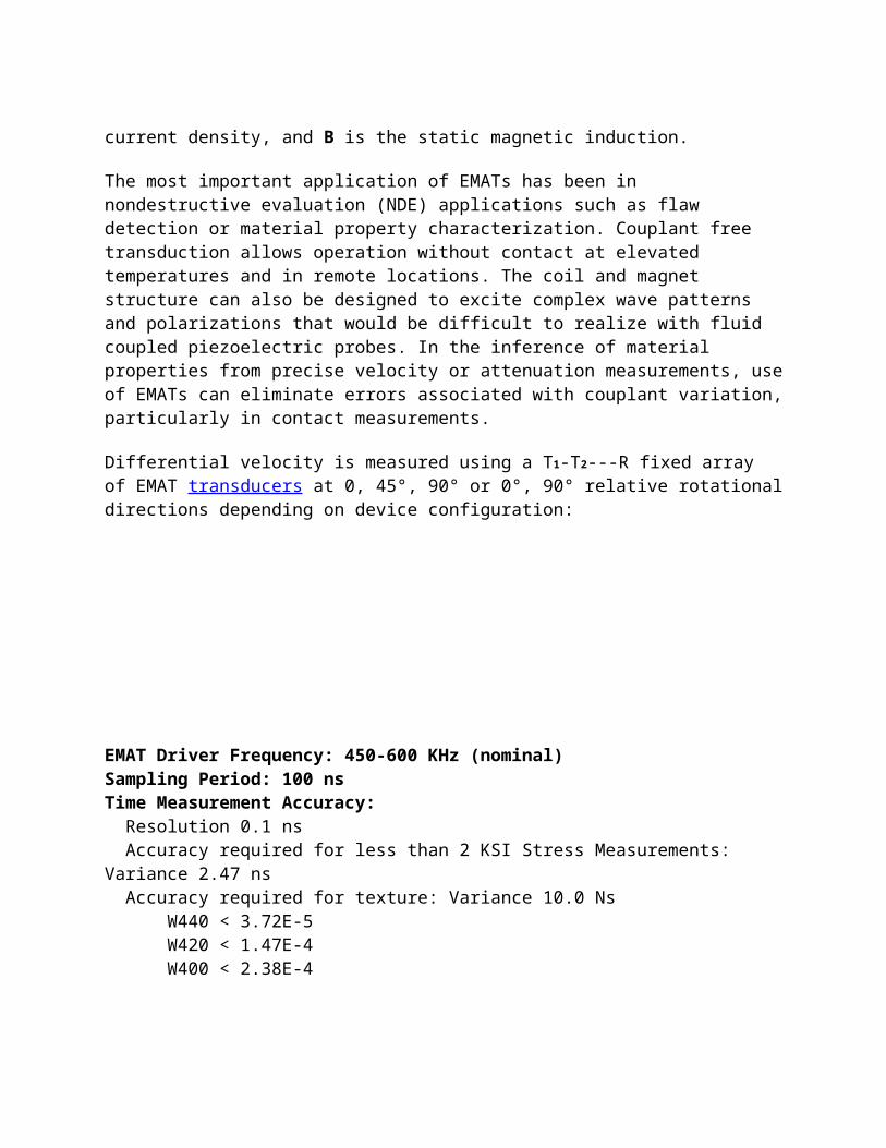
current density, and B is the static magnetic induction.

The most important application of EMATs has been in nondestructive evaluation (NDE) applications such as flaw detection or material property characterization. Couplant free transduction allows operation without contact at elevated temperatures and in remote locations. The coil and magnet structure can also be designed to excite complex wave patterns and polarizations that would be difficult to realize with fluid coupled piezoelectric probes. In the inference of material properties from precise velocity or attenuation measurements, useof EMATs can eliminate errors associated with couplant variation,particularly in contact measurements.

Differential velocity is measured using a T1-T2---R fixed array of EMAT transducers at 0, 45°, 90° or 0°, 90° relative rotationaldirections depending on device configuration:

EMAT Driver Frequency: 450-600 KHz (nominal)Sampling Period: 100 nsTime Measurement Accuracy:--Resolution 0.1 ns--Accuracy required for less than 2 KSI Stress Measurements: Variance 2.47 ns--Accuracy required for texture: Variance 10.0 Ns------W440 < 3.72E-5------W420 < 1.47E-4------W400 < 2.38E-4

Time Measurement Technique

Fourier Transform-Phase-Slope determination of delta time betweenreceived RF bursts (T2-R) - (T1-R), where T2 and T1 EMATs are driven in series to eliminate differential phase shift due to probe liftoff.

Slope of the phase is determined by linear regression of weighteddata points within the signal bandwidth and a weighted y-intercept. The accuracy obtained with this method can exceed one part in one hundred thousand (1:100,000).

Spread Spectrum Ultrasonics

Spread spectrum ultrasonics makes use of the correlation of continuous signals rather than pulse-echo or pitch-catch techniques.

Spread spectrum ultrasonics is a patented new broad band spread-spectrum ultrasonic nondestructive evaluation method. In conventional ultrasonics, a pulse or tone burst is transmitted, then received echoes or through-transmission signals are receivedand analyzed.

In spread spectrum ultrasonics, encoded sound is continuously transmitted into the part or structure being tested. Instead of receiving echoes, spread spectrum ultrasonics generates an acoustic correlation signature having a one-to-one correspondencewith the acoustic state of the part or structure (in its environment) at the instant of the measurement. In its simplest embodiment, the acoustic correlation signature is generated by cross correlating an encoding sequence, with suitable cross and auto correlation properties, transmitted into a part (structure) with received signals returning from the part (structure).

Section of biphase modulated spread spectrum ultrasonic waveform

Multiple probes may be used to ensure that acoustic energy is propagated through all critical volumes of the structure. Triangulation may be incorporated with multiple probes to locate regions of detected distress. Spread spectrum ultrasonics can achieve very high sensitivity to acoustic propagation changes with a low level of energy.

Two significant applications of Spread Spectrum Ultrasonics are:

1. Large Structures that allow ultrasonic transducers to be "permanently" affixed to the structures, eliminating variations in transducer registration and couplant. Comparisons with subsequent acoustic correlation signatures can be used to monitor critical structures such as fracture critical bridge girders. In environments where structures experience a great many variables such as temperature, load,vibration, or environmental coupling, it is necessary to filter out these effects to obtain the correct measurements of defects.

In the example below, simulated defects were created by setting a

couple of steel blocks on the top of the bridge girder.

Trial Setup ContactArea

     Baseline No Flaw --

Flaw 1 One block laying flat on girder 12.5 sq in

Flaw 2 One block standing on its long side 1.25 sq in

Flaw 3 Both blocks standing on their long sides 2.50 sq in

Flaw 4 Both blocks laying flat on girder 25.0 sq in

2. Piece-part assembly line environments where transducers and couplant may be precisely controlled, eliminating significant variations in transducer registration and couplant. Acoustic correlation signatures may be statistically compared to an ensemble of known "good" parts for sorting or accepting/rejectingcriteria in a piece-part assembly line environment.

Impurities in the incoming steel used to forge piece parts may result in sulfite stringer inclusions. In this next example simulated defects were created by placing a magnetized steel wireon the surface of a small steel cylindrical piston used in hydraulic transmissions.

Two discrimination technique are tested here, which are SUF-1 andSUF-2, with the latter giving the best discrimination between defect conditions. The important point being that spread spectrumultrasonics can be extremely sensitive to the acoustic state of apart or structure being tested, and therefore, is a good ultrasonic candidate for testing and monitoring, especially wherescanning is economic unfeasible.

Signal Processing Techniques

Signal processing involves techniques that improve our understanding of information contained in received ultrasonic data. Normally, when a signal is measured with an oscilloscope, it is viewed in the time domain (vertical axis is amplitude or voltage and the horizontal axis is time). For many signals, this is the most logical and intuitive way to view them. Simple signalprocessing often involves the use of gates to isolate the signal of interest or frequency filters to smooth or reject unwanted frequencies.

When the frequency content of the signal is of interest, it makessense to view the signal graph in the frequency domain. In the frequency domain, the vertical axis is still voltage but the horizontal axis is frequency.

-----------Time Domain --------------------Frequency Domain(Magnitude)

The frequency domain display shows how much of the signal's energy is present as a function of frequency. For a simple signalsuch as a sine wave, the frequency domain representation does notusually show us much additional information. However, with more complex signals, such as the response of a broad bandwidth transducer, the frequency domain gives a more useful view of the signal.

Fourier theory says that any complex periodic waveform can be decomposed into a set of sinusoids with different amplitudes, frequencies and phases. The process of doing this is called Fourier Analysis, and the result is a set of amplitudes, phases, and frequencies for each of the sinusoids that makes up the complex waveform. Adding these sinusoids together again will reproduce exactly the original waveform. A plot of the frequency or phase of a sinusoid against amplitude is called a spectrum.

The following Fourier Java applet, adapted with permission of Stanford University, allows the user to manipulate discrete time domain or frequency domain components and see the relationships between signals in time and frequency domains.

The top row (light blue color) represents the real and imaginary

parts of the time domain. Normally the imaginary part of the timedomain signal is identically zero.

The middle row (peach color) represents the the real and imaginary parts of the frequency domain.

The bottom row (light green color) represents the magnitude (amplitude) and phase of the frequency domain signal. Magnitude is the square root of the sum of the squares of the real and imaginary components. Phase is the angular relationship of the real and imaginary components. Ultrasonic transducer manufacturesoften provide plots of both time domain and frequency domain (magnitude) signals characteristic of each transducer. Use this applet to explore the relationship between time and frequency domains.

Exercise: Try replicating time domain signal in the upper left box with a pattern similar to the image on the right. Note the resulting bandwidth in the frequency domain (magnitude) in the lower left box. Next try changing the magnitude, perhaps more of a "mountain" shape tapering to zero. Note that "narrowing" the magnitude, results in more cycles in the time domain signal.

Flaw Reconstruction Techniques

In nondestructive evaluation of structural material defects, the size, shape, and orientation are important flaw parameters in structural integrity assessment. To illustrate flaw reconstruction, a multiviewing ultrasonic transducer system is shown below. A single probe moved sequentially to achieve different perspectives would work equally as well. The apparatus and the signal-processing algorithms were specifically designed at the Center for Nondestructive Evaluation to make use of the theoretical developments in elastic wave scattering in the long and intermediate wavelength regime.

Depicted schematically at the right is the multiprobe system consisting of a sparse array of seven unfocused immersion transducers. This system can be used to "focus" onto a target flaw in a solid by refraction at the surface. The six perimeter transducers are equally spaced on a 5.08 cm diameter ring, surrounding a center transducer. Each of the six perimeter transducers may be independently moved along its axis to allow anequalization of the propagation time for any pitch-catch or pulse-echo combinations. The system currently uses 0.25 in diameter transducers with a nominal center frequency of 10 MHz and a bandwidth extending from approximately 2 to 16 MHz. The axis of the aperture cone of the transducer assembly normally remains vertical and perpendicular to the part surface.

The flaw reconstruction algorithm normally makes use of 13 or 19 backscatter waveforms acquired in a conical pattern within the aperture. The data-acquisition and signal-processing protocol hasfour basic steps.

1. Step one involves the experimental setup, the location and focusing on a target flaw, and acquisition (in a predetermined pattern) of pitch-catch and pulse-echo backscatter waveforms.

2. Step two employs a measurement model to correct the backscatter waveforms for effects of attenuation, diffraction, interface losses, and transducer characteristics, thus resulting in absolute scattering amplitudes.

3. Step three employs a one-dimensional inverse Born approximation to extract a tangent plane to centroid radius estimate for each of the scattering amplitudes.

4. In step four the radius estimates and their corresponding look angles are used in a regression analysis program to determine the six ellipsoidal parameters, three semiaxes, and three Euler angles, defining an ellipsoid which best fits the data.

The inverse Born approximation sizes the flaw by computing the characteristic function of the flaw (defined as unity inside the flaw and zero outside the flaw) as a Fourier transform of the ultrasonic scattering amplitude. The one-dimensional inverse Bornalgorithm treats scattering data in each interrogation direction independently and has been shown to yield the size of ellipsoidalflaws (both voids and inclusions) in terms of the distance from the center of the flaw to the wavefront that is tangent to the front surface of the flaw. Using the multiprobe ultrasonic system, the 1-D inverse Born technique is used to reconstruct voids and inclusions that can be reasonably approximated by an equivalent ellipsoid. So far, the investigation has been confinedto convex flaws with a center of inversion symmetry. The angular scan method described in this paper is capable of locating the bisecting symmetry planes of a flaw. The utility of the multiprobe system is, therefore, expanded since two-dimensional elliptic reconstruction may now be made for the central slice. Additionally, the multiprobe system is well suited for the 3-D flaw reconstruction technique using 2-D slices.

The model-based reconstruction method has been previously appliedto voids and incursion flaws in solids. Since the least-squares regression analysis leading to the "best fit" ellipsoid is based on the tangent plane to centroid distances for the interrogation directions confined within a finite aperture. The success of reconstruction depends on the extent of the flaw surface "illuminated" by the various viewing directions. The extent of coverage of the flaw surface by the tangent plane is a function of the aperture size, flaw shape, and the flaw orientation. For example, a prolate spheroidal flaw with a large aspect ratio

oriented along the axis of the aperture cone will only have one tip illuminated (i.e., covered by the tangent planes) and afford a low reconstruction reliability. For the same reason, orientation of the flaw also has a strong effect on the reconstruction accuracy.

The diagram on the right shows the difference in surface coverageof a tilted flaw and an untilted flaw subjected to the same insonification aperture. Both the experimental and simulation studies of the aperture effect reported before were conducted foroblate and prolate spheroids oriented essentially symmetrically with respect to the part surface and hence the aperture cone. From a flaw reconstruction standpoint, an oblate spheroid with its axis of rotational symmetry perpendicular to the part surfacerepresents a high leverage situation. Likewise, a prolate spheroid with its symmetry axis parallel to the part surface alsoaffords an easier reconstruction than a tilted prolate spheroid. In this CNDE project, we studied effects of flaw orientation on the reconstruction and derived a new data-acquisition approach that will improve reliability of the new reconstruction of arbitrarily oriented flaws.

The orientation of a flaw affects reconstruction results in the following ways.

1. For a given finite aperture, a change in flaw orientation will change the insonified surface area and hence change the"leverage" for reconstruction.

2. The scattering signal amplitude and the signal/noise ratio for any given interrogation direction depends on the flaw orientation.

3. Interference effects, such as those due to tip diffraction phenomena or flash points may be present at certain orientations. Of course, interdependencies exist in these effects, but for the sake of convenience they are discussed separately in the following.

Aperture

To assess the effects of finite aperture size on flaws of

different orientation, computer simulations were performed for anoblate spheroid with semi-axes of 400, 400, and 200 µm that is tilted and untilted with respect to the part surface. For each ofthe 13 scattering directions, the exact radius estimates Re (i.e.the tangent plane to centroid distances) were first computed, anda random error in sizing was then introduced to simulate the experimental situation. The radius estimate used was then taken to be

Re' = Re ( I + n )

where n is a randomly generated number between ±0.1. Using the Re' values for the various directions, a best fit ellipsoid is determined using a regression program. This process is repeated 100 times for each aperture angle and mean standard deviation of the three semiaxes is expressed as a percentage of the expected values. The simulation was performed for the untilted case with the 400 x 400 µm plane parallel to the part surface and for a tilt angle of 40ƒ from the normal of the part surface. The results are summarized in Table I.

The mean values for the ellipsoidal semi-axes converge to expected values, while the standard deviations converge to some asymptotic minimum. The values in Table I show that for a small aperture, the standard deviation as a percentage of expected value (an indication of the reconstruction error) is much higher

for the oblate spheroid tilted at 40ƒ with respect to the horizontal than is the 0ƒ untilted case. As the aperture increases, the difference in reconstruction error approaches zerobecause surface illumination is sufficient to ensure a reliable reconstruction. Due to the combined effect of finite aperture anda prior unknown flaw orientation, a large aperture is desirable to increase reliability of reconstruction results.

Note that in this simulation only the aperture angle is increased, and the number of interrogation directions remains unchanged. The number of look directions is kept the same becausethe multiviewing system is intended for acquiring a sparse array of data based on speed considerations.

Signal/Noise Ratio

For a given scattering direction amplitude of the scattering amplitude and, therefore, the signal/noise ratio depend on orientation of the flaw. In the short wavelength limit scatteringamplitude is proportional to square root of (R1 R2) with R1 and R2 being the principal radii of curvature of the flaw for the scattering direction used. This dependence is found to be important in the intermediate frequency regime as well. To illustrate this effect, the figure at the right shows the scattered signal amplitudes from a football-shaped prolate spheroidal void with two cusp-like tips in two directions: broadside and along the tips. The profile of the tips can increase the ratio of the two signal amplitudes as large as 35.

 

To investigate the correlation between the accuracy of flaw sizing and signal/noise ratio of the flaw waveform at different scattering directions, a 400 x 400 x 200 µm oblate spheroidal void in titanium with its axis of rotational symmetry tilted at a30ƒ angle from normal to the part surface was reconstructed usingthe multiviewing transducer system. It was found that sizing results were generally more accurate for the scattering directions with a higher signal/noise ratio, as expected.

Furthermore, the directions that gave the poorest signal/noise ratios were often ones closest to being in an edge-on perspective. The figure on the right shows the relationship between the percentage error of the radius estimate and signal/noise ratio of the flaw waveform. Reconstruction results of the oblate spheroid void tilted at 30ƒ are listed in Table II.

The reconstruction results of both the semi-axes length and tilt angle were improved by rejecting four data points with the lowestsignal/noise ratios. Since multiviewing transducer system provides a maximum of 19 independent look angles for a given tiltangle of the transducers, rejecting a small subset of the data points based on signal/noise consideration still leaves a sufficient number of data points for the ellipsoidal regression step which requires a minimum of six data points.

Flash Point Interference

The multiview transducer system and associated signal-processing algorithms reconstruct a flaw based on a general ellipsoid model.For ellipsoids with a large aspect ratio and flaw shapes that approach those of a flat crack or a long needle, edge or tip diffractions due to points of stationary phase (flash points)

governed by, geometric acoustics become important. When such phenomena are present within the transducer bandwidth, the scattered signal frequency spectrum contains strong interference maxima and minima and renders radius estimates by the 1-D inverseBorn difficult or impossible.

The figures below show a test flaw in the form of a copper wire segment embedded in a transparent thermoplastic disk and tilted at 45ƒ with respect to the disk surface and the frequency spectrum of the wire inclusion at a scattering angle of 21ƒ from the wire axis. The strong interference pattern prevented the I-D inverse Born algorithm from yielding a meaningful radius estimate. However, when the spectrum was analyzed on assumption of flash point interference (without having to use the angle information), 321 µm was obtained for a path length difference ofthe stationary phase points in the scattering direction; this compared reasonably well with 374 µm for twice the tangent plane distance in this orientation.

----

Photomicrograph of copper wire segment titled at 45ƒ and embeddedin thermoplastic. Each minor division of scale is 10 µm, and wiresegment is approximately prolate spheroid with semi-axes Ax = 80 µm, Ay = 80 µm, and Az = 200 µm.

Spatial Data-acquisition Pattern For Arbitrarily Oriented Flaw

From the investigation described earlier, it is clear that reliable reconstruction of an arbitrarily oriented flaw generallyrequires a large aperture. However, a large viewing aperture perpendicular to the part surface may still contain scattering directions hampered by weak flaw signal amplitude (poor signal-to-noise ratio) and, in certain cases, flash point interference. A predetermined data-acquisition pattern that is relatively free from such disadvantages can improve reconstruction reliability. In this work we explored a method to predetermine a spatial pattern for data acquisition. This pattern affords a high leverage for reliable reconstruction for arbitrarily oriented flaws that can be approximated by the shape of a spheroid.

Consider a tilted prolate spheroid as shown on the right. We may define a vertical sagittal plane (VSP) as the plane that bisects the flaw and contains the z axis. We further define a perpendicular sagittal plane (PSP) as the plane bisecting the spheroid and perpendicular to the VSP. The intersection of the VSP and PSP (direction M in diagram) then corresponds to a direction of maximum flaw signal amplitude. The orientation of the VSP can be located by a series of azimuthal scans at different polar angles. A maximum in the signal amplitude should be observed at the azimuthal angle of the VSP. This definition ofthe VSP and PSP and their relationship to backscattered flaw signal amplitude also holds true for an oblate spheroid. Below shows the azimuthal scans at four different polar angles for the 2.5:1 prolate spheroid (wire segment) flaw. Once the azimuthal angle of the VSP is determined (30ƒ in this case), a polar scan below at the azimuthal angle of the VSP determines the tilt angleof the wire segment to be 41ƒ, as compared to 45ƒ from optical measurement.

----Flaw signal amplitude as a function of azimuthal and polar

angles.

The angular scans serve two very useful functions. First, they provide some information about the shape and orientation of the flaw. For example, a scan in the perpendicular sagittal plane candistinguish a prolate spheroid from an oblate spheroid by changing the polar angle and the azimuthal angle simultaneously. A scan in the PSP of the 2:1 oblate spheroid tilted at 30ƒ showeda peak in flaw signal amplitude at the intersection of the VSP and the PSP (direction M), whereas a scan in the PSP of the tilted 2.5:1 prolate spheroid showed a constant flaw signal amplitude.

Second, it provides a basis for predetermining a spatial data-acquisition pattern that is equivalent to a tilted aperture cone centered at direction M. This data-acquisition pattern not only ensures good signal-to-noise ratio, avoids possible flash point interference due to end-on or edge-on perspectives, and provides a maximum illuminated area on the flaw surface, but also allows one to reconstruct the flaw with two mutually orthogonal elliptical cross sections in the VSP and PSP.

So far, the discussion of angular scans has been confined to

flaws that are approximately spheroidal in shape. For a general ellipsoid with three unequal semi-axes and oriented arbitrarily in space, the angular scan results will be more complicated. For example, an azimuthal scan at different polar angles is not expected to show a peak at the same azimuthal angle. Shape and orientation information, in principle, can still be extracted from such data, and further investigations are underway for the general case.

Reconstruction Results

To verify the reconstruction method using the new spatial data-acquisition configuration experimentally, reconstructions were performed on two test specimens. The first flaw was the 400 µm long 80 µm radius copper wire segment embedded in a thermoplasticdisk. This flaw was used to approximate a prolate spheroid with a2.5:1 aspect ratio. The axis of the wire segment was at a 45ƒ angle relative to the part surface. The second flaw was a 400 x 200 µm oblate spheroidal void tilted at a 30ƒ angle in a diffusion bonded titanium disk, as just described.

The flaw reconstruction procedure using an aperture cone perpendicular to the part surface was first carried out for the 2.5:1 prolate inclusion (copper wire) tilted at a 45ƒ angle. Difficulties due to a poor signal-to-noise ratio and flash point interference associated with look directions close to the end-on perspective prevented a successful reconstruction; in fact, enough inconsistencies occurred in the tangent plane distance estimates that the regression step failed to converge.

Based on orientations of the sagittal planes determined in the angular scans, the new data-acquisition pattern equivalent to tilting the aperture axis to the direction of maximum signal strength was used. The ellipsoidal reconstruction gave a tilt angle of 42ƒ and three semiaxes of 257, 87, and 81 µm. These results compared very favorably with the actual tilt angle of 45ƒand the actual semi-axes of 200, 80, and 80 µm.

The new data-acquisition pattern also allows one to reconstruct an arbitrarily tilted spheroidal flaw with the two mutually orthogonal elliptical cross-sectional cuts in the VSP and PSP. This was done for the copper wire inclusion. After identifying the vertical sagittal plane and the perpendicular sagittal plane,a series of tangent plane distance estimates were made for scattering directions confined in these two planes. Using these results, the two mutually orthogonal elliptical cross sections inthe VSP and PSP were reconstructed using a similar regression program in 2-D. The two reconstructed ellipses were 266 x 83 µm and 80 x 75 µm, respectively, and the tilt angle was found to be 51ƒ. Table III shows the results of the 3-D reconstruction using 19 look perspectives and the 2-D reconstruction of the ellipses in the VSP and PSP. Both reconstructions compared very favorably with the expected values. The greatest discrepancy is in the value of the semi-axis Ax; this is to be expected because the wire segment is approximately a prolate spheroid with two ends truncated.

The 2:1 oblate spheroidal void tilted at a 30ƒ angle in a titanium disk was investigated, again, following the procedure ofpredetermining a favorable data-acquisition pattern based on angular scan results. Table IV shows the reconstruction results using the new data-acquisition pattern equivalent to an aperture cone centered on the direction of maximum backscatter signal. As a comparison, reconstruction results using an aperture cone normal to the part surface (described earlier) are also shown. Ascan be seen, the improvement of the reconstruction by using the new data-acquisition pattern is not as dramatic as the prolate

inclusion case. This is consistent with the fact that the oblate spheroid has a smaller aspect ratio and a smaller tilt angle and is therefore not nearly a "low leverage" flaw to reconstruct using the normal (untilted) data-acquisition pattern.

The reliability problem of reconstructing arbitrarily oriented flaws using the multiviewing transducer system and associated model-based algorithm has been studied. An arbitrarily oriented flaw may afford a low leverage for reconstructing the entire flawbased on limited surface area covered by the tangent planes in a finite aperture and, therefore, requires a greater aperture for areliable reconstruction. However, the aperture size has practicallimits in a single-side access inspection situation and a larger aperture does not necessarily alleviate such difficulties as poorsignal-to-noise ratio and flash point interference associated with certain interrogation directions. In our study of reconstructing approximately spheroidal flaws oriented at some arbitrary angle, it was found beneficial to predetermine a spatial data-acquisition pattern based on angular dependence of the flaw signal amplitude. The new data-acquisition pattern is equivalent to tilting the interrogation aperture cone to compensate for the particular orientation of the flaw and restorethe leverage for a more reliable reconstruction. This method worked well on two test cases.

Calibration Methods

Calibration refers to the act of evaluating and adjusting the precision and accuracy of measurement equipment. In ultrasonic testing, several forms of calibration must occur. First, the electronics of the equipment must be calibrated to ensure that they are performing as designed. This operation is usually

performed by the equipment manufacturer and will not be discussedfurther in this material. It is also usually necessary for the operator to perform a "user calibration" of the equipment. This user calibration is necessary because most ultrasonic equipment can be reconfigured for use in a large variety of applications. The user must "calibrate" the system, which includes the equipment settings, the transducer, and the test setup, to validate that the desired level of precision and accuracy are achieved. The term calibration standard is usually only used whenan absolute value is measured and in many cases, the standards are traceable back to standards at the National Institute for Standards and Technology.

In ultrasonic testing, there is also a need for reference standards. Reference standards are used to establish a general level of consistency in measurements and to help interpret and quantify the information contained in the received signal. Reference standards are used to validate that the equipment and the setup provide similar results from one day to the next and that similar results are produced by different systems. Referencestandards also help the inspector to estimate the size of flaws. In a pulse-echo type setup, signal strength depends on both the size of the flaw and the distance between the flaw and the transducer. The inspector can use a reference standard with an artificially induced flaw of known size and at approximately the same distance away for the transducer to produce a signal. By comparing the signal from the reference standard to that receivedfrom the actual flaw, the inspector can estimate the flaw size.

This section will discuss some of the more common calibration andreference specimen that are used in ultrasonic inspection. Some of these specimens are shown in the figure above. Be aware that there are other standards available and that specially designed standards may be required for many applications. The information provided here is intended to serve a general introduction to the standards and not to be instruction on the proper use of the standards.

Introduction to the Common Standards

Calibration and reference standards for ultrasonic testing come in many shapes and sizes. The type of standard used is dependent on the NDE application and the form and shape of the object beingevaluated. The material of the reference standard should be the same as the material being inspected and the artificially inducedflaw should closely resemble that of the actual flaw. This secondrequirement is a major limitation of most standard reference samples. Most use drilled holes and notches that do not closely represent real flaws. In most cases the artificially induced defects in reference standards are better reflectors of sound energy (due to their flatter and smoother surfaces) and produce indications that are larger than those that a similar sized flaw would produce. Producing more "realistic" defects is cost prohibitive in most cases and, therefore, the inspector can only make an estimate of the flaw size. Computer programs that allow the inspector to create computer simulated models of the part andflaw may one day lessen this limitation.

The IIW Type Calibration Block

The standard shown in the above figure is commonly known in the US as an IIW type reference block. IIW is an acronym for the International Institute of Welding. It is referred to as an IIW "type" reference block because it was patterned after the "true" IIW block but does not conform to IIW requirements in IIS/IIW-23-59. "True" IIW blocks are only made out of steel (to be precise, killed, open hearth or electric furnace, low-carbon steel in the normalized condition with a grain size of McQuaid-Ehn #8) where IIW "type" blocks can be commercially obtained in a selection of

materials. The dimensions of "true" IIW blocks are in metric units while IIW "type" blocks usually have English units. IIW "type" blocks may also include additional calibration and references features such as notches, circular groves, and scales that are not specified by IIW. There are two full-sized and a mini versions of the IIW type blocks. The Mini version is about one-half the size of the full-sized block and weighs only about one-fourth as much. The IIW type US-1 block was derived the basic"true" IIW block and is shown below in the figure on the left. The IIW type US-2 block was developed for US Air Force application and is shown below in the center. The Mini version isshown on the right.

IIW Type US-1

IIW Type US-2

IIW Type Mini

IIW type blocks are used to calibrate instruments for both angle beam and normal incident inspections. Some of their uses include setting metal-distance and sensitivity settings, determining the sound exit point and refracted angle of angle beam transducers, and evaluating depth resolution of normal beam inspection setups.Instructions on using the IIW type blocks can be found in the annex of American Society for Testing and Materials Standard E164, Standard Practice for Ultrasonic Contact Examination of Weldments.

The Miniature Angle-Beam or ROMPAS Calibration Block

The miniature angle-beam is a calibration block that was designedfor the US Air Force for use in the field for instrument calibration. The block is much smaller and lighter than the IIW block but performs many of the same functions. The miniature angle-beam block can be used to check the beam angle and exit point of the transducer. The block can also be used to make metal-distance and sensitivity calibrations for both angle and normal-beam inspection setups.

AWS Shear Wave Distance/Sensitivity Calibration (DSC) Block

A block that closely resembles the miniature angle-beam block andis used in a similar way is the DSC AWS Block. This block is usedto determine the beam exit point and refracted angle of angle-beam transducers and to calibrate distance and set the sensitivity for both normal and angle beam inspection setups. Instructions on using the DSC block can be found in the annex of American Society for Testing and Materials Standard E164, Standard Practice for Ultrasonic Contact Examination of Weldments.

AWS Shear Wave Distance Calibration (DC) Block

The DC AWS Block is a metal path distance and beam exit point calibration standard that conforms to the requirements of the American Welding Society (AWS) and the American Association of State Highway and Transportation Officials (AASHTO). Instructionson using the DC block can be found in the annex of American Society for Testing and Materials Standard E164, Standard Practice for Ultrasonic Contact Examination of Weldments.

AWS Resolution Calibration (RC) Block

The RC Block is used to determine the resolution of angle beam transducers per the requirements of AWS and AASHTO. Engraved Index markers are provided for 45, 60, and 70 degree refracted angle beams.

30 FBH Resolution Reference Block

The 30 FBH resolution reference block is used to evaluate the near-surface resolution and flaw size/depth sensitivity of a normal-beam setup. The block contains number 3 (3/64"), 5 (5/64"), and 8 (8/64") ASTM flat bottom holes at ten metal-distances ranging from 0.050 inch (1.27 mm) to 1.250 inch (31.75 mm).

Miniature Resolution Block

The miniature resolution block is used to evaluate the near-surface resolution and sensitivity of a normal-beam setup It can be used to calibrate high-resolution thickness gages over the range of 0.015 inches (0.381 mm) to 0.125 inches (3.175 mm).

Step and Tapered Calibration Wedges

Step and tapered calibration wedges come in a large variety of sizes and configurations. Step wedges are typically manufactured with four or five steps but custom wedge can be obtained with anynumber of steps. Tapered wedges have a constant taper over the desired thickness range.

Distance/Sensitivity (DS) Block

The DS test block is a calibration standard used to check the horizontal linearity and the dB accuracy per requirements of AWS and AASHTO.

Distance/Area-Amplitude Blocks

-------

Distance/area amplitude correction blocks typically are purchasedas a ten-block set, as shown above. Aluminum sets are manufactured per the requirements of ASTM E127 and steel sets perASTM E428. Sets can also be purchased in titanium. Each block contains a single flat-bottomed, plugged hole. The hole sizes andmetal path distances are as follows:

3/64" at 3" 5/64" at 1/8", 1/4", 1/2", 3/4", 11/2", 3", and 6" 8/64" at 3" and 6"

Sets are commonly sold in 4340 Vacuum melt Steel, 7075-T6 Aluminum, and Type 304 Corrosion Resistant Steel. Aluminum blocks

are fabricated per the requirements of ASTM E127, Standard Practice for Fabricating and Checking Aluminum Alloy Ultrasonic Standard Reference Blocks. Steel blocks are fabricated per the requirements of ASTM E428, Standard Practice for Fabrication and Control of Steel Reference Blocks Used in Ultrasonic Inspection.

Area-Amplitude Blocks

Area-amplitude blocks are also usually purchased in an eight-block set and look very similar to Distance/Area-Amplitude Blocks. However, area-amplitude blocks have a constant 3-inch metal path distance and the hole sizes are varied from 1/64" to 8/64" in 1/64" steps. The blocks are used to determine the relationship between flaw size and signal amplitude by comparing signal responses for the different sized holes. Sets are commonlysold in 4340 Vacuum melt Steel, 7075-T6 Aluminum, and Type 304 Corrosion Resistant Steel. Aluminum blocks are fabricated per therequirements of ASTM E127, Standard Practice for Fabricating and Checking Aluminum Alloy Ultrasonic Standard Reference Blocks. Steel blocks are fabricated per the requirements of ASTM E428, Standard Practice for Fabrication and Control of Steel Reference Blocks Used in Ultrasonic Inspection.

Distance-Amplitude #3, #5, #8 FBH Blocks

Distance-amplitude blocks also very similar to the distance/area-amplitude blocks pictured above. Nineteen block sets with flat-bottom holes of a single size and varying metal path distances are also commercially available. Sets have either a #3 (3/64") FBH, a #5 (5/64") FBH, or a #8 (8/64") FBH. The metal path distances are 1/16", 1/8", 1/4", 3/8", 1/2", 5/8", 3/4", 7/8", 1", 1-1/4", 1-3/4", 2-1/4", 2-3/4", 3-14", 3-3/4", 4-1/4", 4-3/4", 5-1/4", and 5-3/4". The relationship between the metal pathdistance and the signal amplitude is determined by comparing signals from same size flaws at different depth. Sets are commonly sold in 4340 Vacuum melt Steel, 7075-T6 Aluminum, and Type 304 Corrosion Resistant Steel. Aluminum blocks are fabricated per the requirements of ASTM E127, Standard Practice for Fabricating and Checking Aluminum Alloy Ultrasonic Standard

Reference Blocks. Steel blocks are fabricated per the requirements of ASTM E428, Standard Practice for Fabrication and Control of Steel Reference Blocks Used in Ultrasonic Inspection.

istance Amplitude Correction (DAC)

Distance Amplitude Correction (DAC)

Acoustic signals from the same reflecting surface will have different amplitudes at different distances from the transducer. Distance amplitude correction (DAC) provides a means of establishing a graphic ‘reference level sensitivity’ as a function of sweep distance on the A-scan display. The use of DAC allows signals reflected from similar discontinuities to be evaluated where signal attenuation as a function of depth has been correlated. Most often DAC will allow for loss in amplitude over material depth (time), graphically on the A-scan display butcan also be done electronically by certain instruments. Because near field length and beam spread vary according to transducer size and frequency, and materials vary in attenuation and velocity, a DAC curve must be established for each different situation. DAC may be employed in both longitudinal and shear modes of operation as well as either contact or immersion inspection techniques.

A distance amplitude correction curve is constructed from the peak amplitude responses from reflectors of equal area at different distances in the same material. A-scan echoes are displayed at their non-electronically compensated height and the peak amplitude of each signal is marked on the flaw detector screen or, preferably, on a transparent plastic sheet attached tothe screen. Reference standards which incorporate side drilled holes (SDH), flat bottom holes (FBH), or notches whereby the reflectors are located at varying depths are commonly used. It isimportant to recognize that regardless of the type of reflector used, the size and shape of the reflector must be constant. Commercially available reference standards for

constructing DAC include ASTM Distance/Area Amplitude and ASTM E1158 Distance Amplitude blocks, NAVSHIPS Test block, and ASME Basic Calibration Blocks.

The following applet shows a test block with a side drilled hole.The transducer was chosen so that the signal in the shortest pulse-echo path is in the far-field. The transducer may be moved finding signals at depth ratios of 1, 3, 5, and 7. Red points are"drawn" at the peaks of the signals and are used to form the distance amplitude correction curve drawn in blue. Start by pressing the green "Test now!" button. After determining the amplitudes for various path lengths (4), press "Draw DAC" and then press the green "Test now!" button.

 

Thompson-Gray Measurement Model

The Thompson-Gray Measurement Model allows the approximate prediction of ultrasonic scattering measurements made through liquid-solid interfaces. Liquid-solid interfaces are common in physical inspection scenarios. The model allows us to make predictions about received ultrasonic signals scattered from various classes of defects. The model predicts an absolute

scattering amplitude in the sense that amplitudes are correct andtransducer and system characteristics are removed by deconvolution techniques.

Work begun in the early 1980's continues to be refined and has resulted into an increasingly valuable working tool for comparison of ultrasonic theory and experiment. The Thompson-GrayMeasurement Model is at the heart of UTSIM (see section 5.4 Ultrasonic Simulation - UTSIM).

The validity of any model rests on how well its predictions agreewith experiment. Shown below are three examples taken from the J. Acoust. Soc. Am., 74(4) October 1983 entitled, "A model relating ultrasonic scattering measurements through liquid-solid interfaces to unbounded medium scattering amplitudes."

Comparison of theory and experimental magnitude of longitudinal pitch-catch scattering amplitude for a 114 µm radius tin-lead solder sphere in a Lucite cylindrical disk. Illumination was at normal incidence and reception at an 8° angle (15° in the solid).

Comparison of theory and experimental magnitude of longitudinal pitch-catch scattering amplitude for a 114 µm radius tin-lead solder sphere in a Lucite cylindrical disk. Illumination was at normal incidence and reception at an 15.7° angle (30° in the solid).

Comparison of theory and experimental magnitude of longitudinal pitch-catch scattering amplitude for a 114 µm radius tin-lead solder sphere in a Lucite cylindrical disk. Illumination was at normal incidence and reception at a 22.5° angle (45° in the solid).

The relationship between scattering data (obtained from ultrasonic experiments in which the waves are excited and detected in a finite measurement geometry) and unbounded medium, farfield scattering amplitudes, forms the basis of an ultrasonic measurement model.

Geometry of theoretical scattering calculation

For a scatterer in a single fluid medium, a Green's function approach is used to develop an approximate but absolute relationship between these experimental and theoretical cases.

Electromechanical reciprocity relationships are then employed to generalize to a two medium case in which the scatterer is locatedin an elastic solid which, along with the ultrasonic transducer, is immersed in a fluid medium.

The scattering of elastic waves by a flaw in, an unbounded solid,e.g., a crack, void, or inclusion, is often characterized by a scattering amplitude A which defines the spherically spreading wave scattered into the farfield when the flaw is "illuminated" by a unit amplitude plane wave, as schematically illustrated in the above diagram. However, measurements of scattering are alwaysmade with transducers of finite aperture, at finite distances from the scatterer. Furthermore, the transducer is often immersedin a fluid medium and the wave has passed through the liquid-solid interface twice during the measurement.

In principle, complete theoretical scattering solutions can be developed for this more complex scattering situation. However, even the introduction of the liquid-solid interface significantlycomplicates the elastic wave scattering and further introduction of finite beam effects in an exact manner would generally lead tocomputational complexity, which would severely restrict the use of the results in the routine interpretation of experiments.

An alternative point of view would be to view the unbounded medium scattering amplitude A as a canonical solution and to develop approximate expressions, which relate this to the solutions for the more complex measurement geometries. This pointof view is routinely adopted in studies of the acoustic scattering (e.g. sonar) from various obstacles. In this case, theproblem is greatly simplified by the fact that:  (a) the fluid medium only supports a single wave type, (b) the waves do not pass through a refracting and mode converting interface, and (c) calibration experiments can be performed with arbitrary relative positions of transducers and reflecting surfaces to eliminate diffraction effects.

Ultrasonic Simulation - UTSIM

UTSIM is a user interface integrating a CAD model representing a part under inspection and an ultrasound beam model. The beam model can accurately predict fields for focused or planar beams, through curved or flat interfaces in a 3D space. Isotropic materials are required for the current implementation. Within UTSIM, the geometrical boundary conditions are automatically set up when the user points the virtual probe at the 3D solid model. It is fast enough to generate waveforms from flaws in real time.

Grain Noise Modeling

In recent years, a number of theoretical models have been developed at Iowa State University to predict the electrical voltage signals seen during ultrasonic inspections of metal components. For example, the Thompson-Gray measurement model can predict the absolute voltage of the echo from a small defect, given information about the host metal (information such as density, sound speeds, surface curvature, etc.), the defect (size, shape, location, etc.), and the inspection system (water path, transducer characteristics, reference echo from a calibration block, etc.). If an additional metal property which characterizes the inherent noisiness of the metal microstructure is known, the independent scatterer model can be used to predict the absolute root-mean-squared (rms) level of the ultrasonic grain noise seen during an inspection. By combining the two models, signal-to-noise (S/N) ratios can be calculated.

Accurate model calculations often require intensive computer calculations. However, by making a number of approximations in the formalism, it is possible to obtain rapid first-order estimates of noise levels and S/N ratios. These calculations are for normal-incidence pulse-echo inspections through flat or curved surfaces, and the flaw may be a flat crack or a spherical inclusion. The figure below shows the results of one of the calculations.

References & Standards

What are standards?

Standards are documented agreements containing technical specifications or other precise criteria to be used consistently as rules, guidelines, or definitions of characteristics, in orderto ensure that materials, products, processes, and services are fit for their purpose.

For example, the format of the credit cards, phone cards, and "smart" cards that have become commonplace is derived from an ISOInternational Standard. Adhering to the standard, which defines such features as an optimal thickness (0.76 mm), means that the cards can be used worldwide.

An important source of practice codes, standards, and recommendations for NDT is given in the Annual Book of the American Society of Testing and Materials, ASTM.  Volume 03.03, Nondestructive Testing is revised annually, covering acoustic emission, eddy current, leak testing, liquid penetrants, magnetic particle, radiography, thermography, and ultrasonics.

There are many efforts on the part of the National Institute of Standards and Technology (NIST) and other standards organizations, both national and international, to work through technical issues and harmonize national and international standards.

Selected Applications

Rail Inspection

One of the major problems that railroads have faced since the earliest days is the prevention of service failures in track. As is the case with all modes of high-speed travel, failures of an essential component can have serious consequences. The North American railroads have been inspecting their most costly infrastructure asset, the rail, since the late 1920's. With increased traffic at higher speed, and with heavier axle loads inthe 1990's, rail inspection is more important today than it has ever been. Although the focus of the inspection seems like a fairly well-defined piece of steel, the testing variables presentare significant and make the inspection process challenging.

Rail inspections were initially performed solely by visual means.Of course, visual inspections will only detect external defects and sometimes the subtle signs of large internal problems. The need for a better inspection method became a high priority because of a derailment at Manchester, NY in 1911, in which 29 people were killed and 60 were seriously injured. In the U.S. Bureau of Safety's (now the National Transportation Safety Board)investigation of the accident, a broken rail was determined to bethe cause of the derailment. The bureau established that the railfailure was caused by a defect that was entirely internal and probably could not have been detected by visual means. The defect

was called a transverse fissure (example shown on the left). The railroads began investigating the prevalence of this defect and found transverse fissures were widespread.

One of the methods used to inspect rail is ultrasonic inspection.Both normal- and angle-beam techniques are used, as are both pulse-echo and pitch-catch techniques. The different transducer arrangements offer different inspection capabilities. Manual contact testing is done to evaluate small sections of rail but the ultrasonic inspection has been automated to allow inspection of large amounts of rail.

Fluid filled wheels or sleds are often used to couple the transducers to the rail. Sperry Rail Services, which is one of the companies that perform rail inspection, uses Roller Search Units (RSU's) comprising a combination of different transducer angles to achieve the best inspection possible. A schematic of anRSU is shown below.

Weldments (Welded Joints)

The most commonly occurring defects in welded joints are porosity, slag inclusions, lack of side-wall fusion, lack of inter-run fusion, lack of root penetration, undercutting, and longitudinal or transverse cracks.

With the exception of single gas pores all the defects listed areusually well detectable by ultrasonics. Most applications are on low-alloy construction quality steels, however, welds in aluminumcan also be tested. Ultrasonic flaw detection has long been the preferred method for nondestructive testing in welding applications. This safe, accurate, and simple technique has pushed ultrasonics to the forefront of inspection technology.

Ultrasonic weld inspections are typically performed using a straight beam transducer in conjunction with an angle beam transducer and wedge. A straight beam transducer, producing a longitudinal wave at normal incidence into the test piece, is first used to locate any laminations in or near the heat-affectedzone. This is important because an angle beam transducer may not be able to provide a return signal from a laminar flaw.

The second step in the inspection involves using an angle beam transducer to inspect the actual weld. Angle beam transducers usethe principles of refraction and mode conversion to produce refracted shear or longitudinal waves in the test material. [Note: Many AWS inspections are performed using refracted shear waves. However, material having a large grain structure, such as stainless steel may require refracted longitudinal waves for successful inspections.] This inspection may include the root, sidewall, crown, and heat-affected zones of a weld. The process involves scanning the surface of the material around the weldmentwith the transducer. This refracted sound wave will bounce off a reflector (discontinuity) in the path of the sound beam. With proper angle beam techniques, echoes returned from the weld zone may allow the operator to determine the location and type of discontinuity.

To determine the proper scanning area for the weld, the inspectormust first calculate the location of the sound beam in the test material. Using the refracted angle, beam index point and material thickness, the V-path and skip distance of the sound beam is found. Once they have been calculated, the inspector can identify the transducer locations on the surface of the material corresponding to the crown, sidewall, and root of the weld.

-Introduction to

Ultrasonic Testing

IntroductionBasic PrinciplesHistoryPresent StateFuture Direction

Physics of UltrasoundWave PropagationModes of Sound WavesProperties of Plane WavesWavelength/Flaw DetectionElastic Properties of SolidsAttenuationAcoustic ImpedanceReflection/TransmissionRefraction & Snell's LawMode ConversionSignal-to-noise RatioWave Interference

Equipment & TransducersPiezoelectric TransducersCharacteristics of PT Radiated FieldsTransducer Beam SpreadTransducer TypesTransducer Testing ITransducer Testing IITransducer ModelingCouplantEMATsPulser-ReceiversTone Burst GeneratorsFunction GeneratorsImpedance MatchingData Presentation Error Analysis

Measurement TechniquesNormal Beam InspectionAngle Beams IAngle Beams IICrack Tip DiffractionAutomated ScanningVelocity MeasurementsMeasuring AttenuationSpread SpectrumSignal ProcessingFlaw Reconstruction

Calibration MethodsCalibration MethodsDAC CurvesCurvature Correction Thompson-Gray Model

UT Material Properties

Acoustic Properties - Piezoelectric MaterialsAcoustic Properties - Transducers

Acoustic Properties - Metals Acoustic Properties - Powdered Metals Acoustic Properties - Liquid Metals

Acoustic Properties - Plastics, Resins

Acoustic Properties - Rubber

Acoustic Properties - Ceramics

Acoustic Properties - Wood

Acoustic Properties - LiquidsAcoustic Properties - Liquid Gases

Acoustic Properties - Gases Acoustic Properties - Vapors

Acoustic Properties - Body Tissue

UTSIMGrain Noise ModelingReferences/Standards

Selected ApplicationsRail InspectionWeldments

eneral References & Resources

Auld, B.A., Acoustic Fields and Waves in Solids, Vol I & II, 2nd edition Krieger Publishing Company, February 1990; ISBN: 089874783X

Cartz, Louis, Nondestructive Testing : Radiography, Ultrasonics, Liquid Penetrant, Magnetic Particle, Eddy Current, ASM Intl; ISBN: 0871705176

Krautkramer, Josef and Krautkramer, Herbert, Ultrasonic Testing of Materials, 4th/revised edition, Springer Verlag, November 1990, ISBN: 0387512314

Diederichs, Rolf and Ginzel, Ed, Nondestructive Testing Encyclopedia, UT Formulae, NDT net

Ultrasonic Characterization of Materials, NIST, Materials Reliability Division

Ultrasonic Inspection Quizzes

Ready to see how much information on ultrasonic inspection is lock in your brain?  If so, take one of the three quizzes below. These quizzes draw from the same database of questions and differonly in the number of questions presented.  Each time a quiz is opened, a new set of random questions will be produced from the database.  The Collaboration for NDE Education does not record the names of individuals taking a quiz or the results of a quiz.

Ultrasound Quiz 1

   

 ~ First name~    

 ~ Last name~    

1

 

Sound can propagate as:

Longitudinal wavesShear wavesSurface wavesAll of the above

 

2

 

In the transverse or shear wave, the particles:

Move in an elliptical patternOscillate at a right angle to the direction

of wave propagationOscillate parallel to the direction of wave

propagationDo not actually move

 

3

 

Longitudinal waves are also called:

Surface wavesPressure wavesCompressional wavesBoth B and C are correct

 

4

 

Which of the following waves is able to followa surface around a curve?

A longitudinal waveA shear waveA surface waveA Lamb wave

 

5

 

Surface or Rayleigh waves travelling along thesurface of relative thick solid material, penetrate to a depth of approximately:

One wavelengthTwo wavelengthsThree wavelengthsInfinite wavelengths

 

6

 

Shear waves do not propagate in:

SolidsGasesLiquidsBoth B and C are correct

 

7

 

As frequency increases, sound tends to:

Become more compressedScatter more from large or course grain

structureConvert to a different wave modeBecome more penetrating

 

8

 

Which of the following waves is only able to travel through a thin section of material?

A longitudinal waveA shear wavesA surface waveA lamb wave

 

9

 

When sound travels through a medium:

Its intensity diminishes with distanceIt spreads perpendicular to the primary

direction of wave travelIts speed remains constantAll of the above

 

10

 

In order to have a reasonable chance at detecting a discontinuity, the reflective surface of the discontinuity must have a dimension that is at least as long as ________wavelength.

One-halfOneTwo0ne-quarter

 

11  The combined effect of scattering and absorption is called:

Shear factorPropagation

AttenuationImpedance

 

12

 

The terms used to describe a technique�s ability to locate flaws are:

Sensitivity and penetrationSpace and timeSensitivity and resolutionFrequency and size

 

13

 

The ability to locate a small discontinuity iscalled:

ResolutionSensitivityWavelengthFrequency

 

14

 

Acoustic impedance is identified by the letter:

ZIVP

 

15  The ability to locate discontinuities that areclose together within the material is called:

ResolutionSensitivity

EffectivenessPhase delay

 

16

 

When an ultrasound wave passes through an interface between two materials at an oblique angle, and the materials have different indices of refraction, it produces:

Reflected wavesRefracted wavesInterface wavesBoth A and B

 

17

 

Resolution generally increases:

With increased depth of a defectWith a decrease in the transducer frequencyWhen the transducer diameter is reducedWith an increase in transducer frequency

 

18

 

When a wave encounters an interface at an oblique angle, what takes place at the interface due to the different sound velocities of the two materials?

AttenuationRefractionBeam spreadBeam impedance

 

19  The measure of how a signal from a defect compared to other background reflections is

called:

Acoustic impedanceSignal to noise ratioRefractionReflection

 

20

 

Which of the following could influence the behavior of a transducer?

Electrical constructionMaterial constructionMechanical constructionAll of the above

    

    Copyright � The Collaboration for NDT Education..