arX

iv:1

901.

0013

7v3

[cs

.LG

] 2

4 Fe

b 20

20

A Theoretical Analysis of Deep Q-Learning

Jianqing Fan∗ Zhaoran Wang† Yuchen Xie† Zhuoran Yang∗

February 25, 2020

Abstract

Despite the great empirical success of deep reinforcement learning, its theoretical foundation is less

well understood. In this work, we make the first attempt to theoretically understand the deep Q-

network (DQN) algorithm (Mnih et al., 2015) from both algorithmic and statistical perspectives.

In specific, we focus on a slight simplification of DQN that fully captures its key features. Under

mild assumptions, we establish the algorithmic and statistical rates of convergence for the action-

value functions of the iterative policy sequence obtained by DQN. In particular, the statistical

error characterizes the bias and variance that arise from approximating the action-value function

using deep neural network, while the algorithmic error converges to zero at a geometric rate. As a

byproduct, our analysis provides justifications for the techniques of experience replay and target

network, which are crucial to the empirical success of DQN. Furthermore, as a simple extension

of DQN, we propose the Minimax-DQN algorithm for zero-sum Markov game with two players.

Borrowing the analysis of DQN, we also quantify the difference between the policies obtained by

Minimax-DQN and the Nash equilibrium of the Markov game in terms of both the algorithmic

and statistical rates of convergence.

1 Introduction

Reinforcement learning (RL) attacks the multi-stage decision-making problems by interacting with

the environment and learning from the experiences. With the breakthrough in deep learning,

deep reinforcement learning (DRL) demonstrates tremendous success in solving highly challeng-

ing problems, such as the game of Go (Silver et al., 2016, 2017), computer games (Vinyals et al.,

2019), robotics (Kober and Peters, 2012), dialogue systems (Chen et al., 2017). In DRL, the value

or policy functions are often represented as deep neural networks and the related deep learning

techniques can be readily applied. For example, deep Q-network (DQN) (Mnih et al., 2015), asyn-

chronous advantage actor-critic (A3C) (Mnih et al., 2016), trust region policy optimization (TRPO)

(Schulman et al., 2015), proximal policy optimization (PPO) (Schulman et al., 2017) build upon

∗Department of Operations Research and Financial Engineering, Princeton University. Research supported by the

NSF grant DMS-1662139 and DMS-1712591, the ONR grant N00014-19-1-2120, and the NIH grant 2R01-GM072611-

14.†Department of Industrial Engineering and Management Sciences, Northwestern University

1

classical RL methods (Watkins and Dayan, 1992; Sutton et al., 2000; Konda and Tsitsiklis, 2000)

and have become benchmark algorithms for artificial intelligence.

Despite its great empirical success, there exists a substantial gap between the theory and prac-

tice of DRL. In particular, most existing theoretical work on reinforcement learning focuses on the

tabular case where the state and action spaces are finite, or the case where the value function is

linear. Under these restrictive settings, the algorithmic and statistical perspectives of reinforcement

learning are well-understood via the tools developed for convex optimization and linear regression.

However, in presence of nonlinear function approximators such as deep neural network, the theoret-

ical analysis of reinforcement learning becomes intractable as it involves solving a highly nonconvex

statistical optimization problem.

To bridge such a gap in DRL, we make the first attempt to theoretically understand DQN,

which can be cast as an extension of the classical Q-learning algorithm (Watkins and Dayan, 1992)

that uses deep neural network to approximate the action-value function. Although the algorithmic

and statistical properties of the classical Q-learning algorithm are well-studied, theoretical analysis

of DQN is highly challenging due to its differences in the following two aspects.

First, in online gradient-based temporal-difference reinforcement learning algorithms, approx-

imating the action-value function often leads to instability. Baird (1995) proves that this is the

case even with linear function approximation. The key technique to achieve stability in DQN is

experience replay (Lin, 1992; Mnih et al., 2015). In specific, a replay memory is used to store the

trajectory of the Markov decision process (MDP). At each iteration of DQN, a mini-batch of states,

actions, rewards, and next states are sampled from the replay memory as observations to train the

Q-network, which approximates the action-value function. The intuition behind experience replay

is to achieve stability by breaking the temporal dependency among the observations used in training

the deep neural network.

Second, in addition to the aforementioned Q-network, DQN uses another neural network named

the target network to obtain an unbiased estimator of the mean-squared Bellman error used in

training the Q-network. The target network is synchronized with the Q-network after each period

of iterations, which leads to a coupling between the two networks. Moreover, even if we fix the

target network and focus on updating the Q-network, the subproblem of training a neural network

still remains less well-understood in theory.

In this paper, we focus on a slight simplification of DQN, which is amenable to theoretical anal-

ysis while fully capturing the above two aspects. In specific, we simplify the technique of experience

replay with an independence assumption, and focus on deep neural networks with rectified linear

units (ReLU) (Nair and Hinton, 2010) and large batch size. Under this setting, DQN is reduced to

the neural fitted Q-iteration (FQI) algorithm (Riedmiller, 2005) and the technique of target net-

work can be cast as the value iteration. More importantly, by adapting the approximation results

for ReLU networks to the analysis of Bellman operator, we establish the algorithmic and statistical

rates of convergence for the iterative policy sequence obtained by DQN. As shown in the main

results in §3, the statistical error characterizes the bias and variance that arise from approximating

the action-value function using neural network, while the algorithmic error geometrically decays to

zero as the number of iteration goes to infinity.

2

Furthermore, we extend DQN to two-player zero-sum Markov games (Shapley, 1953). The

proposed algorithm, named Minimax-DQN, can be viewed as a combination of the Minimax-Q

learning algorithm for tabular zero-sum Markov games (Littman, 1994) and deep neural networks

for function approximation. Compared with DQN, the main difference lies in the approaches to

compute the target values. In DQN, the target is computed via maximization over the action

space. In contrast, the target obtained computed by solving the Nash equilibrium of a zero-sum

matrix game in Minimax-DQN, which can be efficiently attained via linear programming. Despite

such a difference, both these two methods can be viewed as approximately applying the Bellman

operator to the Q-network. Thus, borrowing the analysis of DQN, we also establish theoretical

results for Minimax-DQN. Specifically, we quantify the suboptimality of policy returned by the

algorithm by the difference between the action-value functions associated with this policy and with

the Nash equilibrium policy of the Markov game. For this notion of suboptimality, we establish the

both algorithmic and statistical rates of convergence, which implies that the action-value function

converges to the optimal counterpart up to an unimprovable statistical error in geometric rate.

Our contribution is three-fold. First, we establish the algorithmic and statistical errors of

the neural FQI algorithm, which can be viewed as a slight simplification of DQN. Under mild

assumptions, our results show that the proposed algorithm obtains a sequence of Q-networks that

geometrically converges to the optimal action-value function up to an intrinsic statistical error

induced by the approximation bias of ReLU network and finite sample size. Second, as a byproduct,

our analysis justifies the techniques of experience replay and target network used in DQN, where the

latter can be viewed as a single step of the value iteration. Third, we propose the Minimax-DQN

algorithm that extends DQN to two-player zero-sum Markov games. Borrowing the analysis for

DQN, we establish the algorithmic and statistical convergence rates of the action-value functions

associated with the sequence of policies returned by the Minimax-DQN algorithm.

1.1 Related Works

There is a huge body of literature on deep reinforcement learning, where these algorithms are based

on Q-learning or policy gradient (Sutton et al., 2000). We refer the reader to Arulkumaran et al.

(2017) for a survey of the recent developments of DRL. In addition, the DQN algorithm is first

proposed in Mnih et al. (2015), which applies DQN to Artari 2600 games (Bellemare et al., 2013).

The extensions of DQN include double DQN (van Hasselt et al., 2016), dueling DQN (Wang et al.,

2016), deep recurrent Q-network (Hausknecht and Stone, 2015), asynchronous DQN (Mnih et al.,

2016), and variants designed for distributional reinforcement learning (Bellemare et al., 2017; Dabney et al.,

2018b,a). All of these algorithms are corroborated only by numerical experiments, without theo-

retical guarantees. Moreover, these algorithms not only inherit the tricks of experience replay and

the target network proposed in the original DQN, but develop even more tricks to enhance the

performance. Furthermore, recent works such as Schaul et al. (2016); Andrychowicz et al. (2017);

Liu and Zou (2018); Zhang and Sutton (2017); Novati and Koumoutsakos (2019) study the effect

of experience replay and propose various modifications.

In addition, our work is closely related to the literature on batch reinforcement learning (Lange et al.,

2012), where the goal is to estimate the value function given transition data. These problems

3

are usually formulated into least-squares regression, for which various algorithms are proposed

with finite-sample analysis. However, most existing works focus on the settings where the value

function are approximated by linear functions. See Bradtke and Barto (1996); Boyan (2002);

Lagoudakis and Parr (2003); Lazaric et al. (2016); Farahmand et al. (2010); Lazaric et al. (2012);

Tagorti and Scherrer (2015) and the references therein for results of the least-squares policy itera-

tion (LSPI) and Bellman residue minimization (BRM) algorithms. Beyond linear function approx-

imation, a recent work (Farahmand et al., 2016) studies the performance of LSPI and BRM when

the value function belongs to a reproducing kernel Hilbert space. However, we study the fitted Q-

iteration algorithm, which is a batch RL counterpart of DQN. The fitted Q-iteration algorithm is

proposed in Ernst et al. (2005), and Riedmiller (2005) proposes the neural FQI algorithm. Finite-

sample bounds for FQI have been established in Murphy (2005); Munos and Szepesvari (2008) for

large classes of regressors. However, their results are not applicable to ReLU networks due to

the huge capacity of deep neural networks. Furthermore, various extensions of FQI are studied in

Antos et al. (2008a); Farahmand et al. (2009); Tosatto et al. (2017); Geist et al. (2019) to handle

continuous actions space, ensemble learning, and entropy regularization. The empirical perfor-

mances of various batch RL methods have been examined in Levine et al. (2017); Agarwal et al.

(2019); Fujimoto et al. (2019).

Moreover, Q-learning, and reinforcement learning methods in general, have been widely applied

to dynamic treatment regimes (DTR) (Chakraborty, 2013; Laber et al., 2014; Tsiatis, 2019), where

the goal is to find sequential decision rules for individual patients that adapt to time-evolving

illnesses. There is a huge body of literature on this line of research. See, e.g., Murphy (2003);

Zhao et al. (2009); Qian and Murphy (2011); Zhao et al. (2011); Zhang et al. (2012); Zhao et al.

(2012); Goldberg and Kosorok (2012); Nahum-Shani et al. (2012); Goldberg et al. (2013); Schulte et al.

(2014); Song et al. (2015); Zhao et al. (2015); Linn et al. (2017); Zhou et al. (2017); Shi et al. (2018);

Zhu et al. (2019) and the references therein. Our work provides a theoretical underpinning for the

application of DQN to DTR (Liu et al., 2019b) and motivates the principled usage of DRL methods

in healthcare applications (Yu et al., 2019).

Furthermore, our work is also related to works that apply reinforcement learning to zero-sum

Markov games. The Minimax-Q learning is proposed by Littman (1994), which is an online algo-

rithm that is an extension Q-learning. Subsequently, for Markov games, various online algorithms

are also proposed with theoretical guarantees. These works consider either the tabular case or lin-

ear function approximation. See, e.g., Bowling (2001); Conitzer and Sandholm (2007); Prasad et al.

(2015); Wei et al. (2017); Perolat et al. (2018); Srinivasan et al. (2018); Wei et al. (2017) and the

references therein. In addition, batch reinforcement learning is also applied to zero-sum Markov

games by Lagoudakis and Parr (2002); Perolat et al. (2015, 2016a,b); Zhang et al. (2018), which

are closely related to our work. All of these works consider either linear function approximation

or a general function class with bounded pseudo-dimension (Anthony and Bartlett, 2009). How-

ever, there results cannot directly imply finite-sample bounds for Minimax-DQN due to the huge

capacity of deep neural networks.

Finally, our work is also related a line of research on the model capacity of ReLU deep neural

networks, which leads to understanding the generalization property of deep learning (Mohri et al.,

4

2012; Kawaguchi et al., 2017). Specifically, Bartlett (1998); Neyshabur et al. (2015b,a); Bartlett et al.

(2017); Golowich et al. (2018); Liang et al. (2019) propose various norms computed from the net-

works parameters and establish capacity bounds based upon these norms. In addition, Maass

(1994); Bartlett et al. (1999); Schmidt-Hieber (2020+); Bartlett et al. (2019); Klusowski and Barron

(2016); Barron and Klusowski (2018); Suzuki (2019); Bauer et al. (2019) study the Vapnik-Chervonenkis

(VC) dimension of neural networks and Dziugaite and Roy (2017); Neyshabur et al. (2018) estab-

lish the PAC-Bayes bounds for neural networks. Among these works, our work is more related to

Schmidt-Hieber (2020+); Suzuki (2019), which relate the VC dimension of the ReLU networks to

a set of hyperparameters used to define the networks. Based on the VC dimension, they study the

statistical error of nonparametric regression using ReLU networks. In sum, theoretical understand-

ing of deep learning is pertinent to the study of DRL algorithms. See Kawaguchi et al. (2017);

Neyshabur et al. (2017); Fan et al. (2019) and the references therein for recent developments on

theoretical analysis of the generalization property of deep learning.

1.2 Notation

For a measurable space with domain S, we denote by B(S, V ) the set of measurable functions on

S that are bounded by V in absolute value. Let P(S) be the set of all probability measures over

S. For any ν ∈ P(S) and any measurable function f : S → R, we denote by ‖f‖ν,p the ℓp-norm

of f with respect to measure ν for p ≥ 1. In addition, for simplicity, we write ‖f‖ν for ‖f‖2,ν . In

addition, let {f(n), g(n)}n≥1 be two positive series. We write f(n) . g(n) if there exists a constant

C such that f(n) ≤ C · g(n) for all n larger than some n0 ∈ N. In addition, we write f(n) ≍ g(n)

if f(n) . g(n) and g(n) . f(n).

2 Background

In this section, we introduce the background. We first lay out the formulation of the reinforcement

learning problem, and then define the family of ReLU neural networks.

2.1 Reinforcement Learning

A discounted Markov decision process is defined by a tuple (S,A, P,R, γ). Here S is the set of all

states, which can be countable or uncountable, A is the set of all actions, P : S × A → P(S) is

the Markov transition kernel, R : S × A → P(R) is the distribution of the immediate reward, and

γ ∈ (0, 1) is the discount factor. In specific, upon taking any action a ∈ A at any state s ∈ S,P (· | s, a) defines the probability distribution of the next state and R(· | s, a) is the distribution of

the immediate reward. Moreover, for regularity, we further assume that S is a compact subset

of Rr which can be infinite, A = {a1, a2, . . . , aM} has finite cardinality M , and the rewards are

uniformly bounded by Rmax, i.e., R(· |s, a) has a range on [−Rmax, Rmax] for any s ∈ S and a ∈ A.A policy π : S → P(A) for the MDP maps any state s ∈ S to a probability distribution π(· | s)

over A. For a given policy π, starting from the initial state S0 = s, the actions, rewards, and states

5

evolve according to the law as follows:{(At, Rt, St+1) : At ∼ π(· |St), Rt ∼ R(· |St, At), St+1 ∼ P (· | St, At)

}, t = 0, 1, · · · ,

and the corresponding value function V π : S → R is defined as the cumulative discounted reward

obtained by taking the actions according to π when starting from a fixed state, that is,

V π(s) = E

[ ∞∑

t=0

γt ·Rt∣∣∣∣S0 = s

]. (2.1)

The policy π can be controlled by decision makers, yet the functions P and R are given by the

nature or the system that are unknown to decision makers.

By the law of iterative expectation, for any policy π,

V π(s) = E[Qπ(s,A)

∣∣A ∼ π(· | s)], ∀s ∈ S, (2.2)

where Qπ(s, a), called an action value function, is given by

Qπ(s, a) = E

[ ∞∑

t=0

γt · Rt∣∣∣∣S0 = s,A0 = a

]= r(s, a) + γ · E

[V π(S′)

∣∣S′ ∼ P (· | s, a)], (2.3)

with r(s, a) =∫rR(dr | s, a) is the expected reward at state s given action a. Moreover, we define

an operator P π by

(P πQ)(s, a) = E[Q(S′, A′)

∣∣S′ ∼ P (· | s, a), A′ ∼ π(· |S′)], (2.4)

and define the Bellman operator T π by (T πQ)(s, a) = r(s, a) + γ · (P πQ)(s, a). Then Qπ in (2.3) is

the unique fixed point of T π.

The goal of reinforcement learning is to find the optimal policy, which achieves the largest

cumulative reward via dynamically learning from the acquired data. To characterize optimality, by

(2.2), we naturally define the optimal action-value function Q∗ as

Q∗(s, a) = supπQπ(s, a), ∀(s, a) ∈ S ×A. (2.5)

where the supremum is taken over all policies. In addition, for any given action-value function

Q : S×A → R, we define the greedy policy πQ as any policy that selects the action with the largest

Q-value, that is, for any s ∈ S, πQ(· |s) satisfies

πQ(a | s) = 0 if Q(s, a) 6= maxa′∈A

Q(s, a′). (2.6)

Based on Q∗, we define the optimal policy π∗ as any policy that is greedy with respect to Q∗. It

can be shown that Q∗ = Qπ∗. Finally, we define the Bellman optimality operator T via

(TQ)(s, a) = r(s, a) + γ · E[maxa′∈A

Q(S′, a′)∣∣S′ ∼ P (· | s, a)

]. (2.7)

Then we have the Bellman optimality equation TQ∗ = Q∗.

6

Furthermore, it can be verified that the Bellman operator T is γ-contractive with respect to

the supremum norm over S × A. That is, for any two action-value functions Q,Q′ : S × A → R,

it holds that ‖TQ − TQ′‖∞ ≤ γ · ‖Q − Q′‖∞. Such a contraction property yields the celebrated

value iteration algorithm (Sutton and Barto, 2011), which constructs a sequence of action-value

functions {Qk}k≥0 by letting Qk = TQk−1 for all k ≥ 1, where the initialization function Q0 is

arbitrary. Then it holds that ‖Qk−Q∗‖∞ ≤ γk ·‖Q0−Q∗‖∞, i.e., {Qk}k≥0 converges to the optimal

value function at a linear rate. This approach forms the basis of the neural FQI algorithm, where

the Bellman operator is empirically learned from a batch of data dynamically and the action-value

functions are approximated by deep neural networks.

2.2 Deep Neural Network

We study the performance of DQN with rectified linear unit (ReLU) activation function σ(u) =

max(u, 0). For any positive integer L and {dj}L+1i=0 ⊆ N, a ReLU network f : Rd0 → R

dL+1 with L

hidden layers and width {dj}L+1i=0 is of form

f(x) =WL+1σ(WLσ(WL−1 . . . σ(W2σ(W1x+ v1) + v2) . . . vL−1) + vL), (2.8)

where Wℓ ∈ Rdℓ×dℓ−1 and vℓ ∈ R

dℓ are the weight matrix and the shift (bias) vector in the ℓ-th

layer, respectively. Here we apply σ to to each entry of its argument in (2.8). In deep learning, the

network structure is fixed, and the goal is to learn the network parameters (weights) {Wℓ, vℓ}ℓ∈[L+1]

with the convention that vL+1 = 0. For deep neural networks, the number of parameters greatly

exceeds the input dimension d0. To restrict the model class, we focus on the class of ReLU networks

where most parameters are zero.

Definition 2.1 (Sparse ReLU Network). For any L, s ∈ N, {dj}L+1i=0 ⊆ N , and V > 0, the family

of sparse ReLU networks bounded by V with L hidden layers, network width d, and weight sparsity

s is defined as

F(L, {dj}L+1i=0 , s, V ) =

{f : max

ℓ∈[L+1]‖Wℓ‖∞ ≤ 1,

L+1∑

ℓ=1

‖Wℓ‖0 ≤ s, maxj∈[dL+1]

‖fj‖∞ ≤ V}, (2.9)

where we denote (Wℓ, vℓ) by Wℓ. Moreover, f in (2.9) is expressed as in (2.8), and fj is the j-th

component of f .

Here we focus on functions that are uniformly bounded because the value functions in (2.1)

and (2.3) are always bounded by Vmax = Rmax/(1 − γ). We also assume that the network weights

are uniformly bounded and bounded by one without loss of generality. In the sequel, we write

F(L, {dj}L+1j=0 , s, Vmax) as F(L, {dj}L+1

j=0 , s) to simplify the notation. In addition, we restrict the

networks weights to be sparse, i.e., s is much smaller compared with the total number of pa-

rameters. Such an assumption implies that the network has sparse connections, which are useful

for applying deep learning in memory-constrained situations such as mobile devices (Han et al.,

2016; Liu et al., 2015). Empirically, sparse neural networks are realized via various regularization

techniques such as Dropout (Srivastava et al., 2014), which randomly sets a fixed portion of the

7

network weights to zero. Moreover, sparse network architectures have recently been advocated by

the intriguing lottery ticket hypothesis (Frankle and Carbin, 2019), which states that each dense

network has a subnetwork with the sparse connections, when trained in isolation, achieves compa-

rable performance as the original network. Thus, focusing on the class of sparse ReLU networks

does not sacrifice the statistical accuracy.

Moreover, we introduce the notion of Holder smoothness as follows, which is a generalization of

Lipschitz continuity, and is widely used to characterize the regularity of functions.

Definition 2.2 (Holder Smooth Function). Let D be a compact subset of Rr, where r ∈ N. We

define the set of Holder smooth functions on D as

Cr(D, β,H) =

{f : D → R :

∑

α : |α|<β‖∂αf‖∞ +

∑

α : ‖α‖1=⌊β⌋sup

x,y∈D,x 6=y

|∂αf(x)− ∂α(y)|‖x− y‖β−⌊β⌋

∞≤ H

},

where β > 0 andH > 0 are parameters and ⌊β⌋ is the largest integer no greater than β. In addition,

here we use the multi-index notation by letting α = (α1, . . . , αr)⊤ ∈ N

r, and ∂α = ∂α1 . . . ∂αr .

Finally, we conclude this section by defining functions that can be written as a composition

of multiple Holder functions, which captures complex mappings in real-world applications such as

multi-level feature extraction.

Definition 2.3 (Composition of Holder Functions). Let q ∈ N and {pj}j∈[q] ⊆ N be integers, and

let {aj , bj}j∈[q] ⊆ R such that aj < bj j ∈ [q]. Moreover, let gj : [aj, bj ]pj → [aj+1, bj+1]

pj+1 be a

function, ∀j ∈ [q]. Let (gjk)k∈[pj+1] be the components of gj , and we assume that each gjk is Holder

smooth, and depends on at most tj of its input variables, where tj could be much smaller than pj ,

i.e., gjk ∈ Ctj ([aj , bj ]tj , βj ,Hj). Finally, we denote by G({pj , tj , βj ,Hj}j∈[q]) the family of functions

that can be written as compositions of {gj}j∈[q], with the convention that pq+1 = 1. That is, for

any f ∈ G({pj , tj, βj ,Hj}j∈[q]), we can write

f = gq ◦ gq−1 ◦ . . . ◦ g2 ◦ g1, (2.10)

with gjk ∈ Ctj ([aj , bj ]tj , βj ,Hj) for each k ∈ [pj+1] and j ∈ [q].

Here f in (2.10) is a composition of q vector-valued mappings {gj}j∈[q] where each gj has pj+1

components and its k-th component, gjk, ∀k ∈ [pj+1], is a Holder smooth function defined on

[aj , bj ]pj . Moreover, it is well-known the statistical rate for estimating a Holder smooth function

depends on the input dimension (Tsybakov, 2008). Here we assume that gjk only depends on tj of

its inputs, where tj ∈ [pj] can be much smaller than pj, which enables us to obtain a more refined

analysis that adapts to the effective smoothness of f . In particular, Definition 2.3 covers the family

of Holder smooth functions and the additive model (Friedman and Stuetzle, 1981) on [0, 1]r as two

special cases, where the former suffers from the curse of dimensionality whereas the latter does not.

3 Understanding Deep Q-Network

In the DQN algorithm, a deep neural network Qθ : S×A→ R is used to approximate Q∗, where θ isthe parameter. For completeness, we state DQN as Algorithm 3 in §A. As shown in the experiments

in (Mnih et al., 2015), two tricks are pivotal for the empirical success of DQN.

8

First, DQN use the trick of experience replay (Lin, 1992). Specifically, at each time t, we

store the transition (St, At, Rt, St+1) into the replay memory M, and then sample a minibatch of

independent samples from M to train the neural network via stochastic gradient descent. Since

the trajectory of MDP has strong temporal correlation, the goal of experience replay is to obtain

uncorrelated samples, which yields accurate gradient estimation for the stochastic optimization

problem.

Another trick is to use a target network Qθ⋆ with parameter θ⋆ (current estimate of parameter).

With independent samples {(si, ai, ri, s′i)}i∈[n] from the replay memory (we use s′i instead of si+1

for the next state right after si and ai to avoid notation crash with next independent sample si+1

in the state space), to update the parameter θ of the Q-network, we compute the target

Yi = ri + γ ·maxa∈A

Qθ⋆(s′i, a)

(compare with Bellman optimality operator (2.7)), and update θ by the gradient of

L(θ) =1

n

n∑

i=1

[Yi −Qθ(si, ai)]2. (3.1)

Whereas parameter θ⋆ is updated once every Ttarget steps by letting θ⋆ = θ. That is, the target

network is hold fixed for Ttarget steps and then updated it by the current weights of the Q-network.

To demystify DQN, it is crucial to understand the role played by these two tricks. For experience

replay, in practice, the replay memory size is usually very large. For example, the replay memory size

is 106 in Mnih et al. (2015). Moreover, DQN use the ǫ-greedy policy, which enables exploration over

S ×A. Thus, when the replay memory is large, experience replay is close to sampling independent

transitions from an explorative policy. This reduces the variance of the ∇L(θ), which is used to

update θ. Thus, experience replay stabilizes the training of DQN, which benefits the algorithm in

terms of computation.

To understand the statistical property of DQN, we replace the experience replay by sampling

independent transitions from a given distribution σ ∈ P(S ×A). That is, instead of sampling from

the replay memory, we sample i.i.d. observations {(Si, Ai)}i∈[n] from σ. Moreover, for any i ∈ [n],

let Ri and S′i be the immediate reward and the next state when taking action Ai at state Si. Under

this setting, we have E(Yi |Si, Ai) = (TQθ⋆)(Si, Ai), where T is the Bellman optimality operator in

(2.7) and Qθ⋆ is the target network.

Furthermore, to further understand the necessity of the target network, let us first neglect the

target network and set θ⋆ = θ. Using bias-variance decomposition, the the expected value of L(θ)

in (3.1) is

E[L(θ)

]= ‖Qθ − TQθ‖2σ + E

{[Y1 − (TQθ)(S1, A1)

]2}. (3.2)

Here the first term in (3.2) is known as the mean-squared Bellman error (MSBE), and the second

term is the variance of Y1. Whereas L(θ) can be viewed as the empirical version of the MSBE,

which has bias E{[Y1− (TQθ)(S1, A1)]2} that also depends on θ. Thus, without the target network,

minimizing L(θ) can be drastically different from minimizing the MSBE.

9

To resolve this problem, we use a target network in (3.1), which has expectation

E[L(θ)

]= ‖Qθ − TQθ∗‖2σ + E

{[Y1 − (TQθ∗)(S1, A1)

]2},

where the variance of Y1 does not depend on θ. Thus, minimizing L(θ) is close to solving

minimizeθ∈Θ

‖Qθ − TQθ⋆‖2σ, (3.3)

where Θ is the parameter space. Note that in DQN we hold θ⋆ still and update θ for Ttarget steps.

When Ttarget is sufficiently large and we neglect the fact that the objective in (3.3) is nonconvex,

we would update θ by the minimizer of (3.3) for fixed θ⋆.

Therefore, in the ideal case, DQN aims to solve the minimization problem (3.3) with θ⋆ fixed, and

then update θ⋆ by the minimizer θ. Interestingly, this view of DQN offers a statistical interpretation

of the target network. In specific, if {Qθ : θ ∈ Θ} is sufficiently large such that it contains TQθ⋆ , then

(3.3) has solution Qθ = TQθ⋆ , which can be viewed as one-step of value iteration (Sutton and Barto,

2011) for neural networks. In addition, in the sample setting, Qθ⋆ is used to construct {Yi}i∈[n],which serve as the response in the regression problem defined in (3.1), with (TQθ⋆) being the

regression function.

Furthermore, turning the above discussion into a realizable algorithm, we obtain the neural

fitted Q-iteration (FQI) algorithm, which generates a sequence of value functions. Specifically, let

F be a class of function defined on S ×A. In the k-th iteration of FQI, let Qk be current estimate

of Q∗. Similar to (3.1) and (3.3), we define Yi = Ri + γ ·maxa∈A Qk(S′i, a), and update Qk by

Qk+1 = argminf∈F

1

n

n∑

i=1

[Yi − f(Si, Ai)

]2. (3.4)

This gives the fitted-Q iteration algorithm, which is stated in Algorithm 1.

The step of minimization problem in (3.4) essentially finds Qk+1 in F such that Qk+1 ≈ TQk.

Let us denote Qk+1 = TkQk where Tk is an approximation of the Bellman optimality operator

T learned from the training data in the k-th iteration. With the above notation, we can now

understand our Algorithm 1 as follows. Starting from the initial estimator Q0, collect the data

{(Si, Ai, Ri, S′i)}i∈[n] and learn the map T1 via (3.4) and get Q1 = T1Q0. Then, get a new batch

of sample and learn the map T2 and get Q2 = T2Q1, and so on. Our final estimator of the action

value is QK = TK · · · T1Q0, which resembles the updates of the value iteration algorithm at the

population level.

When F is the family of neural networks, Algorithm 1 is known as the neural FQI algorithm,

which is proposed in Riedmiller (2005). Thus, we can view neural FQI as a modification of DQN,

where we replace experience replay with sampling from a fixed distribution σ, so as to understand

the statistical property. As a byproduct, such a modification naturally justifies the trick of target

network in DQN. In addition, note that the optimization problem in (3.4) appears in each iteration

of FQI, which is nonconvex when neural networks are used. However, since we focus solely on the

statistical aspect, we make the assumption that the global optima of (3.4) can be reached, which is

also contained F . Interestingly, a recent line of research on deep learning (Du et al., 2019b,a;

10

Zou et al., 2018; Chizat et al., 2019; Allen-Zhu et al., 2019a,b; Jacot et al., 2018; Cao and Gu,

2019; Arora et al., 2019; Weinan et al., 2019; Mei et al., 2019; Yehudai and Shamir, 2019) has es-

tablished global convergence of gradient-based algorithms for empirical risk minimization when

the neural networks are overparametrized. We provide more discussions on the computation as-

pect in §B. Furthermore, we make the i.i.d. assumption in Algorithm 1 to simplify the analysis.

Antos et al. (2008b) study the performance of fitted value iteration with fixed data used in the

regression sub-problems repeatedly, where the data is sampled from a single trajectory based on

a fixed policy such that the induced Markov chain satisfies certain conditions on the mixing time.

Using similar analysis as in Antos et al. (2008b), our algorithm can also be extended to handled

fixed data that is collected beforehand.

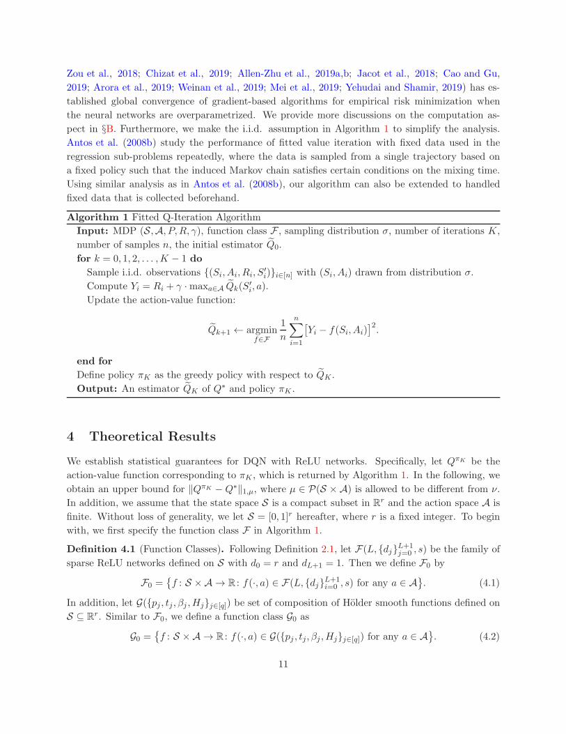
Algorithm 1 Fitted Q-Iteration Algorithm

Input: MDP (S,A, P,R, γ), function class F , sampling distribution σ, number of iterations K,

number of samples n, the initial estimator Q0.

for k = 0, 1, 2, . . . ,K − 1 do

Sample i.i.d. observations {(Si, Ai, Ri, S′i)}i∈[n] with (Si, Ai) drawn from distribution σ.

Compute Yi = Ri + γ ·maxa∈A Qk(S′i, a).

Update the action-value function:

Qk+1 ← argminf∈F

1

n

n∑

i=1

[Yi − f(Si, Ai)

]2.

end for

Define policy πK as the greedy policy with respect to QK .

Output: An estimator QK of Q∗ and policy πK .

4 Theoretical Results

We establish statistical guarantees for DQN with ReLU networks. Specifically, let QπK be the

action-value function corresponding to πK , which is returned by Algorithm 1. In the following, we

obtain an upper bound for ‖QπK −Q∗‖1,µ, where µ ∈ P(S × A) is allowed to be different from ν.

In addition, we assume that the state space S is a compact subset in Rr and the action space A is

finite. Without loss of generality, we let S = [0, 1]r hereafter, where r is a fixed integer. To begin

with, we first specify the function class F in Algorithm 1.

Definition 4.1 (Function Classes). Following Definition 2.1, let F(L, {dj}L+1j=0 , s) be the family of

sparse ReLU networks defined on S with d0 = r and dL+1 = 1. Then we define F0 by

F0 ={f : S × A → R : f(·, a) ∈ F(L, {dj}L+1

i=0 , s) for any a ∈ A}. (4.1)

In addition, let G({pj , tj , βj ,Hj}j∈[q]) be set of composition of Holder smooth functions defined on

S ⊆ Rr. Similar to F0, we define a function class G0 as

G0 ={f : S × A → R : f(·, a) ∈ G({pj , tj, βj ,Hj}j∈[q]) for any a ∈ A

}. (4.2)

11

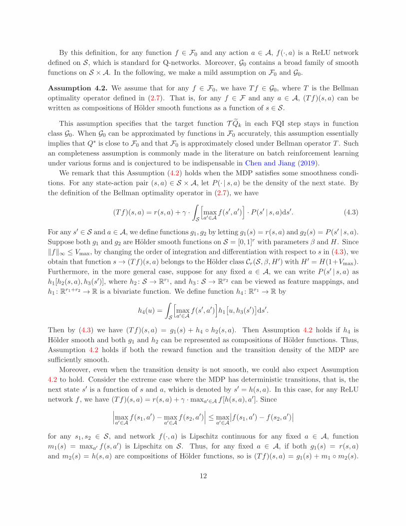
By this definition, for any function f ∈ F0 and any action a ∈ A, f(·, a) is a ReLU network

defined on S, which is standard for Q-networks. Moreover, G0 contains a broad family of smooth

functions on S × A. In the following, we make a mild assumption on F0 and G0.

Assumption 4.2. We assume that for any f ∈ F0, we have Tf ∈ G0, where T is the Bellman

optimality operator defined in (2.7). That is, for any f ∈ F and any a ∈ A, (Tf)(s, a) can be

written as compositions of Holder smooth functions as a function of s ∈ S.

This assumption specifies that the target function T Qk in each FQI step stays in function

class G0. When G0 can be approximated by functions in F0 accurately, this assumption essentially

implies that Q∗ is close to F0 and that F0 is approximately closed under Bellman operator T . Such

an completeness assumption is commonly made in the literature on batch reinforcement learning

under various forms and is conjectured to be indispensable in Chen and Jiang (2019).

We remark that this Assumption (4.2) holds when the MDP satisfies some smoothness condi-

tions. For any state-action pair (s, a) ∈ S × A, let P (· | s, a) be the density of the next state. By

the definition of the Bellman optimality operator in (2.7), we have

(Tf)(s, a) = r(s, a) + γ ·∫

S

[maxa′∈A

f(s′, a′)]· P (s′ | s, a)ds′. (4.3)

For any s′ ∈ S and a ∈ A, we define functions g1, g2 by letting g1(s) = r(s, a) and g2(s) = P (s′ | s, a).Suppose both g1 and g2 are Holder smooth functions on S = [0, 1]r with parameters β and H. Since

‖f‖∞ ≤ Vmax, by changing the order of integration and differentiation with respect to s in (4.3), we

obtain that function s→ (Tf)(s, a) belongs to the Holder class Cr(S, β,H ′) with H ′ = H(1+Vmax).

Furthermore, in the more general case, suppose for any fixed a ∈ A, we can write P (s′ | s, a) as

h1[h2(s, a), h3(s′)], where h2 : S → R

r1 , and h3 : S → Rr2 can be viewed as feature mappings, and

h1 : Rr1+r2 → R is a bivariate function. We define function h4 : R

r1 → R by

h4(u) =

∫

S

[maxa′∈A

f(s′, a′)]h1

[u, h3(s

′)]ds′.

Then by (4.3) we have (Tf)(s, a) = g1(s) + h4 ◦ h2(s, a). Then Assumption 4.2 holds if h4 is

Holder smooth and both g1 and h2 can be represented as compositions of Holder functions. Thus,

Assumption 4.2 holds if both the reward function and the transition density of the MDP are

sufficiently smooth.

Moreover, even when the transition density is not smooth, we could also expect Assumption

4.2 to hold. Consider the extreme case where the MDP has deterministic transitions, that is, the

next state s′ is a function of s and a, which is denoted by s′ = h(s, a). In this case, for any ReLU

network f , we have (Tf)(s, a) = r(s, a) + γ ·maxa′∈A f [h(s, a), a′]. Since∣∣∣maxa′∈A

f(s1, a′)−max

a′∈Af(s2, a

′)∣∣∣ ≤ max

a′∈A

∣∣f(s1, a′)− f(s2, a′)∣∣

for any s1, s2 ∈ S, and network f(·, a) is Lipschitz continuous for any fixed a ∈ A, function

m1(s) = maxa′ f(s, a′) is Lipschitz on S. Thus, for any fixed a ∈ A, if both g1(s) = r(s, a)

and m2(s) = h(s, a) are compositions of Holder functions, so is (Tf)(s, a) = g1(s) +m1 ◦m2(s).

12

Therefore, even if the MDP has deterministic dynamics, when both the reward function r(s, a) and

the transition function h(s, a) are sufficiently nice, Assumption 4.2 still holds true.

In the following, we define the concentration coefficients, which measures the similarity between

two probability distributions under the MDP.

Assumption 4.3 (Concentration Coefficients). Let ν1, ν2 ∈ P(S×A) be two probability measures

that are absolutely continuous with respect to the Lebesgue measure on S × A. Let {πt}t≥1 be a

sequence of policies. Suppose the initial state-action pair (S0, A0) of the MDP has distribution ν1,

and we take action At according to policy πt. For any integer m, we denote by P πmP πm−1 · · ·P π1ν1the distribution of {(St, At)}mt=0. Then we define the m-th concentration coefficient as

κ(m; ν1, ν2) = supπ1,...,πm

[Eν2

∣∣∣∣d(P πmP πm−1 · · ·P π1ν1)

dν2

∣∣∣∣2]1/2

, (4.4)

where the supremum is taken over all possible policies.

Furthermore, let σ be the sampling distribution in Algorithm 1 and let µ be a fixed distribution

on S × A. We assume that there exists a constant φµ,σ <∞ such that

(1− γ)2 ·∑

m≥1

γm−1 ·m · κ(m;µ, σ) ≤ φµ,σ, (4.5)

where (1− γ)2 in (4.5) is a normalization term, since∑

m≥1 γm−1 ·m = (1− γ)−2.

By definition, concentration coefficients in (4.4) quantifies the similarity between ν2 and the

distribution of the future states of the MDP when starting from ν1. Moreover, (4.5) is a stan-

dard assumption in the literature. See, e.g., Munos and Szepesvari (2008); Lazaric et al. (2016);

Scherrer et al. (2015); Farahmand et al. (2010, 2016). This assumption holds for large class of

systems MDPs and specifically for MDPs whose top-Lyapunov exponent is finite. Moreover, this

assumption essentially requires that the sampling distribution σ has sufficient coverage over S ×Aand is shown to be necessary for the success of batch RL methods (Chen and Jiang, 2019). See

Munos and Szepesvari (2008); Antos et al. (2007); Chen and Jiang (2019) for more detailed discus-

sions on this assumption.

Now we are ready to present the main theorem.

Theorem 4.4. Under Assumptions 4.2 and 4.3, let F0 be defined in (4.1) based on the family of

sparse ReLU networks F(L∗, {d∗j}L∗+1

j=0 , s∗) and let G0 be given in (4.2) with {Hj}j∈[q] being absoluteconstants. Moreover, for any j ∈ [q − 1], we define β∗j = βj ·

∏ℓ=j+1min(βℓ, 1); let β

∗q = 1. In

addition, let α∗ = maxj∈[q] tj/(2β∗j + tj). For the parameters of G0, we assume that the sample size

n is sufficiently large such that there exists a constant ξ > 0 satisfying

max

{ q∑

j=1

(tj + βj + 1)3+tj ,∑

j∈[q]log(tj + βj), max

j∈[q]pj

}. (log n)ξ. (4.6)

For the hyperparameters L∗, {d∗j}L∗+1

j=0 , and s∗ of the ReLU network, we set d∗0 = 0 and d∗L∗+1 = 1.

Moreover, we set

L∗ . (log n)ξ∗

, r ≤ minj∈[L∗]

d∗j ≤ maxj∈[L∗]

d∗j . nξ∗

, and s∗ ≍ nα∗ · (log n)ξ∗ (4.7)

13

for some constant ξ∗ > 1+2ξ. For any K ∈ N, let QπK be the action-value function corresponding

to policy πK , which is returned by Algorithm 1 based on function class F0. Then there exists a

constant C > 0 such that

‖Q∗ −QπK‖1,µ ≤ C ·φµ,σ · γ(1− γ)2 · |A| · (log n)

1+2ξ∗ · n(α∗−1)/2 +4γK+1

(1− γ)2 · Rmax. (4.8)

This theorem implies that the statistical rate of convergence is the sum of a statistical error

and an algorithmic error. The algorithmic error converges to zero in linear rate as the algorithm

proceeds, whereas the statistical error reflects the fundamental difficulty of the problem. Thus,

when the number of iterations satisfy

K ≥ C ′ ·[log |A|+ (1− α∗) · log n

]/ log(1/γ)

iterations, where C ′ is a sufficiently large constant, the algorithmic error is dominated by the

statistical error. In this case, if we view both γ and φµ,σ as constants and ignore the polylogarithmic

term, Algorithm 1 achieves error rate

|A| · n(α∗−1)/2 = |A| ·maxj∈[q]

n−β∗j /(2β

∗j +tj), (4.9)

which scales linearly with the capacity of the action space, and decays to zero when the n goes to

infinity. Furthermore, the rates {n−β∗j /(2β

∗j +tj)}j∈[q] in (4.9) recovers the statistical rate of nonpara-

metric regression in ℓ2-norm, whereas our statistical rate n(α∗−1)/2 in (4.9) is the fastest among

these nonparametric rates, which illustrates the benefit of compositional structure of G0.Furthermore, as a concrete example, we assume that both the reward function and the Markov

transition kernel are Holder smooth with smoothness parameter β. As stated below Assumption

4.2, for any f ∈ F0, we have (Tf)(·, a) ∈ Cr(S, β,H ′). Then Theorem 4.4 implies that Algorithm 1

achieves error rate |A| ·n−β/(2β+r) when K is sufficiently large. Since |A| is finite, this rate achievesthe minimax-optimal statistical rate of convergence within the class of Holder smooth functions

defined on [0, 1]d (Stone, 1982) and thus cannot be further improved. As another example, when

(Tf)(·, a) ∈ Cr(S, β,H ′) can be represented as an additive model over [0, 1]r where each component

has smoothness parameter β, (4.9) reduces to |A| ·n−β/(2β+1), which does not depends on the input

dimension r explicitly. Thus, by having a composite structure in G0, Theorem 4.4 yields more refined

statistical rates that adapt to the intrinsic difficulty of solving each iteration of Algorithm 1.

In the sequel, we conclude this section by sketching the proof of Theorem 4.4; the detailed proof

is deferred to §6.

Proof Sketch of Theorem 4.4. Recall that πk is the greedy policy with respect to Qk and QπK is

the action-value function associated with πK , whose definition is given in (2.3). Since {Qk}k∈[K] is

constructed by a iterative algorithm, it is crucial to relate ‖Q∗−QπK‖1,µ, the quantity of interest, to

the errors incurred in the previous steps, namely {Qk − TQk−1}k∈[K]. Thus, in the first step of the

proof, we establish Theorem 6.1, also known as the error propagation (Munos and Szepesvari, 2008;

Lazaric et al., 2016; Scherrer et al., 2015; Farahmand et al., 2010, 2016) in the batch reinforcement

14

learning literature, which provides an upper bound on ‖Q∗−QπK‖1,µ using {‖Qk−TQk−1‖σ}k∈[K].

In particular, Theorem 6.1 asserts that

‖Q∗ −QπK‖1,µ ≤2φµ,σ · γ(1− γ)2 · max

k∈[K]‖Qk − TQk−1‖σ +

4γK+1

(1− γ)2 · Rmax, (4.10)

where φµ,σ, given in (4.5), is a constant that only depends on distributions µ and σ.

The upper bound in (4.10) shows that the total error of Algorithm 1 can be viewed as a sum

of a statistical error and an algorithmic error, where maxk∈[K] ‖Qk − TQk−1‖σ is essentially the

statistical error and the second term on the right-hand side of (4.10) corresponds to the algorithmic

error. Here, the statistical error diminishes as the sample size n in each iteration grows, whereas the

algorithmic error decays to zero geometrically as the number of iterations K increases. This implies

that the fundamental difficulty of DQN is captured by the error incurred in a single step. Moreover,

the proof of this theorem depends on bounding Qℓ−TQℓ−1 using Qk−TQk−1 for any k < ℓ, which

characterizes how the one-step error Qk − TQk−1 propagates as the algorithm proceeds. See §C.1for a detailed proof.

It remains to bound ‖Qk − TQk−1‖σ for any k ∈ [K]. We achieve such a goal using tools from

nonparametric regression. Specifically, as we will show in Theorem 6.2, under Assumption 4.2, for

any k ∈ [K] we have

‖Qk+1 − TQk‖2σ ≤ 4 · [dist∞(F0,G0)]2 + C · V 2max/n · logNδ + C · Vmax · δ (4.11)

for any δ > 0, where C > 0 is an absolute constant,

dist∞(F0,G0) = supf ′∈G0

inff∈F0

‖f − f ′‖∞ (4.12)

is the ℓ∞-error of approximating functions in G0 using functions in F0, and Nδ is the minimum

number of cardinality of the balls required to cover F0 with respect to ℓ∞-norm.

Furthermore, (4.11) characterizes the bias and variance that arise in estimating the action-value

functions using deep ReLU networks. Specifically, [dist∞(F0,G0)]2 corresponds to the bias incurred

by approximating functions in G0 using ReLU networks. We note that such a bias is measured in

the ℓ∞-norm. In addition, V 2max/n · logNδ + Vmax · δ controls the variance of the estimator.

In the sequel, we fix δ = 1/n in (4.11), which implies that

‖Qk+1 − TQk‖2σ ≤ 4 · dist2∞(F0,G0) + C ′ · V 2max/n · logNδ, (4.13)

where C ′ > 0 is an absolute constant.

In the subsequent proof, we establish upper bounds for dist(F0,G0) defined in (4.12) and logNδ,

respectively. Recall that the family of composite Holder smooth functions G0 is defined in (4.2).

By the definition of G0 in (4.2), for any f ∈ G0 and any a ∈ A, f(·, a) ∈ G({(pj , tj, βj ,Hj)}j∈[q])is a composition of Holder smooth functions, that is, f(·, a) = gq ◦ · · · ◦g1. Recall that, as defined in

Definition 2.3, gjk is the k-th entry of the vector-valued function gj . Here gjk ∈ Ctj ([aj , bj ]tj , βj ,Hj)

for each k ∈ [pj+1] and j ∈ [q]. To construct a ReLU network that is f(·, a), we first show that f(·, a)

15

can be reformulated as a composition of Holder functions defined on a hypercube. Specifically, let

h1 = g1/(2H1) + 1/2, hq(u) = gq(2Hq−1u−Hq−1), and

hj(u) = gj(2Hj−1u−Hj−1)/(2Hj) + 1/2

for all j ∈ {2, . . . , q − 1}. Then we immediately have

f(·, a) = gq ◦ · · · ◦ g1 = hq ◦ · · · ◦ h1. (4.14)

Furthermore, by the definition of Holder smooth functions in Definition 2.2, for any j ∈ [q] and

k ∈ [pj+1], it is not hard to verify that hjk ∈ Ctj([0, 1]tj ,W

), where we define W > 0 by

W = max{

max1≤j≤q−1

(2Hj−1)βj ,Hq(2Hq−1)

βq}, (4.15)

Now we employ Lemma 6.3, obtained from Schmidt-Hieber (2020+), to construct a ReLU

network that approximates each hjk, which, combined with (4.14), yields a ReLU network that is

close to f(·, a) in the ℓ∞-norm.

To apply Lemma 6.3 we set m = η · ⌈log2 n⌉ for a sufficiently large constant η > 1, and set N

to be a sufficiently large integer that depends on n, which will be specified later. In addition, we

set Lj = 8+ (m+ 5) · (1 + ⌈log2(tj + βj)⌉). Then, by Lemma 6.3, there exists a ReLU network hjksuch that ‖hjk − hjk‖∞ . N−βj/tj . Furthermore, we have hjk ∈ F(Lj , {tj , dj , . . . , dj , 1}, sj), with

dj = 6(tj + ⌈βj⌉)N, sj ≤ 141 · (tj + βj + 1)3+tj ·N · (m+ 6). (4.16)

Now we define f : S → R by f = hq ◦ · · · ◦ h1 and set

N =⌈max1≤j≤q

C · ntj/(2β∗j +tj)

⌉. (4.17)

For this choice of N , we show that f belongs to function class F(L∗, {d∗j}L∗+1

j=1 , s∗). Moreover, we

define λj =∏qℓ=j+1(βℓ ∧ 1) for any j ∈ [q − 1], and set λq = 1. Then we have βj · λj = β∗j for all

j ∈ [q]. Furthermore, we show that f is a good approximation of f(·, a). Specifically, we have

‖f(·, a)− f‖∞ .

q∑

j=1

‖hj − hj‖λj∞.

Combining this with (4.17) and the fact that ‖hjk − hjk‖∞ . N−βj/tj , we obtain that

[dist(F0,G0)

]2. nα

∗−1. (4.18)

Moreover, using classical results on the covering number of neural networks (Anthony and Bartlett,

2009), we further show that

logNδ . |A| · s∗ · L∗ maxj∈[L∗]

log(d∗j ) . |A| · nα∗ · (log n)1+2ξ∗ , (4.19)

where δ = 1/n. Therefore, combining (4.11), (4.13), (4.18), and (4.19), we conclude the proof.

16

5 Extension to Two-Player Zero-Sum Markov Games

In this section, we propose the Minimax-DQN algorithm, which combines DQN and the Minimax-

Q learning for two-player zero-sum Markov games. We first present the background of zero-sum

Markov games and introduce the the algorithm in §5.1. Borrowing the analysis for DQN in the

previous section, we provide theoretical guarantees for the proposed algorithm in §5.2.

5.1 Minimax-DQN Algorithm

As one of the simplistic extension of MDP to the multi-agent setting, two-player zero-sum Markov

game is denoted by (S,A,B, P,R, γ), where S is state space, A and B are the action spaces of the

first and second player, respectively. In addition, P : S × A× B → P(S) is the Markov transition

kernel, and R : S × A × B → P(R) is the distribution of immediate reward received by the first

player. At any time t, the two players simultaneously take actions At ∈ A and Bt ∈ B at state

St ∈ S, then the first player receives reward Rt ∼ R(St, At, Bt) and the second player obtains −Rt.The goal of each agent is to maximize its own cumulative discounted return.

Furthermore, let π : S → P(A) and ν : S → P(B) be policies of the first and second players,

respectively. Then, we similarly define the action-value function Qπ,ν : S × A× B → R as

Qπ,ν(s, a, b) = E

[ ∞∑

t=0

γt · Rt∣∣∣∣ (S0, A0, B0) = (s, a, b), At ∼ π(· |St), Bt ∼ ν(· |St)

], (5.1)

and define the state-value function V π,ν : S → R as

V π,ν(s) = E[Qπ,ν(s,A,B)

∣∣A ∼ π(· | s), B ∼ ν(· | s)]. (5.2)

Note that these two value functions are defined by the rewards of the first player. Thus, at any state-

action tuple (s, a, b), the two players aim to solve maxπminν Qπ,ν(s, a, b) and minν maxπQ

π,ν(s, a, b),

respectively. By the von Neumann’s minimax theorem (Von Neumann and Morgenstern, 1947;

Patek, 1997), there exists a minimax function of the game, Q∗ : S × A× B → R, such that

Q∗(s, a, b) = maxπ

minνQπ,ν(s, a, b) = min

νmaxπ

Qπ,ν(s, a, b). (5.3)

Moreover, for joint policy (π, ν) of two players, we define the Bellman operators T π,ν and T by

(T π,νQ)(s, a, b) = r(s, a, b) + γ · (P π,νQ)(s, a, b), (5.4)

(TQ)(s, a, b) = r(s, a, b) + γ · (P ∗Q)(s, a, b), (5.5)

where r(s, a, b) =∫rR(dr | s, a, b), and we define operators P π,ν and P ∗ by

(P π,νQ)(s, a, b) = Es′∼P (· | s,a,b),a′∼π(· | s′),b′∼ν(· | s′)[Q(s′, a′, b′)

],

(P ∗Q)(s, a, b) = Es′∼P (· | s,a,b){

maxπ′∈P(A)

minν′∈P(B)

Ea′∼π′,b′∼ν′[Q(s′, a′, b′)

]}.

Note that P ∗ is defined by solving a zero-sum matrix game based on Q(s′, ·, ·) ∈ R|A|×|B|, which

could be achieved via linear programming. It can be shown that both T π,ν and T are γ-contractive,

17

with Qπ,ν defined in (5.1) and Q∗ defined in (5.3) being the unique fixed points, respectively.

Furthermore, similar to (2.6), in zero-sum Markov games, for any action-value function Q, the

equilibrium joint policy with respect to Q is defined as

[πQ(· | s), νQ(· | s)

]= argmax

π′∈P(A)argminν′∈P(B)

Ea∼π′,b∼ν′[Q(s, a, b)

], ∀s ∈ S. (5.6)

That is, πQ(· | s) and νQ(· | s) solves the zero-sum matrix game based on Q(s, ·, ·) for all s ∈ S. Bythis definition, we obtain that the equilibrium joint policy with respect to the minimax function

Q∗ defined in (5.3) achieves the Nash equilibrium of the Markov game.

Therefore, to learn the Nash equilibrium, it suffices to estimate Q∗, which is the unique fixed

point of the Bellman operator T . Similar to the standard Q-learning for MDP, Littman (1994)

proposes the Minimax-Q learning algorithm, which constructs a sequence of action-value functions

that converges to Q∗. Specifically, in each iteration, based on a transition (s, a, b, s′), Minimax-Q

learning updates the current estimator of Q∗, denoted by Q, via

Q(s, a, b)← (1− α) ·Q(s, a, b) + α ·{r(s, a, b) + γ · max

π′∈P(A)min

ν′∈P(B)Ea′∼π′,b′∼ν′

[Q(s′, a′, b′)

]},

where α ∈ (0, 1) is the stepsize.

Motivated by this algorithm, we propose the Minimax-DQN algorithm which extend DQN to

two-player zero-sum Markov games. Specifically, we parametrize the action-value function using

a deep neural network Qθ : S × A × B → R and store the transition (St, At, Bt, Rt, St+1) into the

replay memoryM at each time-step. Parameter θ of the Q-network is updated as follows. Let Qθ∗

be the target network. With n independent samples {(si, ai, bi, ri, s′i)}i∈[n] fromM, for all i ∈ [n],

we compute the target

Yi = ri + γ · maxπ′∈P(A)

minν′∈P(B)

Ea∼π′,b∼ν′[Qθ∗(s

′i, a, b)

], (5.7)

which can be attained via linear programming. Then we update θ in the direction of ∇θL(θ), whereL(θ) = n−1

∑i∈[n][Yi−Qθ(si, ai, bi)]2. Finally, the target network Qθ∗ is updated every Ttarget steps

by letting θ∗ = θ. For brevity, we defer the details of Minimax-DQN to Algorithm 4 in §A.

To understand the theoretical aspects of this algorithm, we similarly utilize the framework of

batch reinforcement learning for statistical analysis. With the insights gained in §3, we consider

a modification of Minimax-DQN based on neural fitted Q-iteration, whose details are stated in

Algorithm 2. As in the MDP setting, we replace sampling from the replay memory by sampling

i.i.d. state-action tuples from a fixed distribution σ ∈ P(S × A × B), and estimate Q∗ in (5.3)

by solving a sequence of least-squares regression problems specified by (5.8). Intuitively, this

algorithm approximates the value iteration algorithm for zero-sum Markov games (Littman, 1994)

by constructing a sequence of value functions {Qk}k≥0 such that Qk+1 ≈ TQk for all k, where T

defined in (5.5) is the Bellman operator.

5.2 Theoretical Results for Minimax-FQI

Following the theoretical results established in §4, in this subsection, we provide statistical guar-

antees for the Minimax-FQI algorithm with F being a family of deep neural networks with ReLU

18

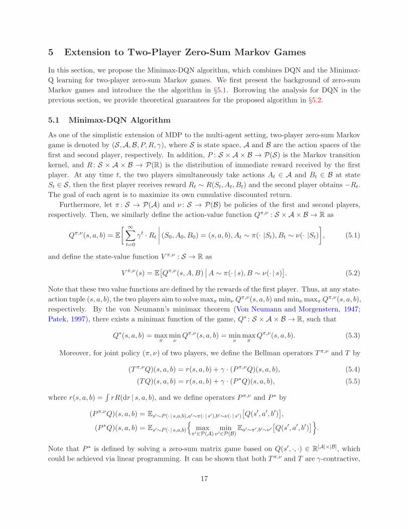
Algorithm 2 Fitted Q-Iteration Algorithm for Zero-Sum Markov Games (Minimax-FQI)

Input: Two-player zero-sum Markov game (S,A,B, P,R, γ), function class F , distribution σ ∈P(S × A× B), number of iterations K, number of samples n, the initial estimator Q0 ∈ F .for k = 0, 1, 2, . . . ,K − 1 do

Sample n i.i.d. observations {(Si, Ai, Bi)}i∈[n] from σ, obtain Ri ∼ R(· |Si, Ai, Bi) and S′i ∼

P (· |Si, Ai, Bi).Compute Yi = Ri + γ ·maxπ′∈P(A) minν′∈P(B) Ea∼π′,b∼ν′

[Qk(s

′i, a, b)

].

Update the action-value function:

Qk+1 ← argminf∈F

1

n

n∑

i=1

[Yi − f(Si, Ai, Bi)

]2. (5.8)

end for

Let (πK , νK) be the equilibrium joint policy with respect to QK , which is defined in (5.6).

Output: An estimator QK of Q∗ and joint policy (πK , νK).

activation. Hereafter, without loss of generality, we assume S = [0, 1]r with r being a fixed integer,

and the action spaces A and B are both finite. To evaluate the performance of the algorithm, we

first introduce the best-response policy as follows.

Definition 5.1. For any policy π : S → P(A) of player one, the best-response policy against π,

denoted by ν∗π, is defined as the optimal policy of second player when the first player follows π. In

other words, for all s ∈ S, we have ν∗π(· | s) = argminν Vπ,ν(s), where V π,ν is defined in (5.2).

Note that when the first player adopt a fixed policy π, from the perspective of the second

player, the Markov game becomes a MDP. Thus, ν∗π is the optimal policy of the MDP induced by

π. Moreover, it can be shown that, for any policy π, Q∗(s, a, b) ≥ Qπ,ν∗π(s, a, b) holds for every state-

action tuple (s, a, b). Thus, by considering the adversarial case where the opponent always plays

the best-response policy, the difference between Qπ.ν∗π and Q∗ servers as a characterization of the

suboptimality of π. Hence, to quantify the performance of Algorithm 2, we consider the closeness

between Q∗ and QπK ,ν∗πK , which will be denoted by Q∗

K hereafter for simplicity. Specifically, in the

following we establish an upper bound for ‖Q∗ −Q∗K‖1,µ for some distribution µ ∈ P(S × A× B).

We first specify the function class F in Algorithm 2 as follows.

Assumption 5.2 (Function Classes). Following Definition 4.1, let F(L, {dj}L+1j=0 , s) and G({pj , tj, βj ,Hj}j∈[q])

be the family of sparse ReLU networks and the set of composition of Holder smooth functions de-

fined on S, respectively. Similar to (4.1), we define F1 by

F1 ={f : S × A× B → R : f(·, a, b) ∈ F(L, {dj}L+1

i=0 , s) for any (a, b) ∈ A× B}. (5.9)

For the Bellman operator T defined in (5.5), we assume that for any f ∈ F1 and any state-action

tuple (s, a, b), we have (Tf)(·, a, b) ∈ G({pj , tj, βj ,Hj}j∈[q]).

19

We remark that this Assumption is in the same flavor as Assumption 4.2. As discussed in §4,this assumption holds if both the reward function and the transition density of the Markov game

are sufficiently smooth.

In the following, we define the concentration coefficients for Markov games.

Assumption 5.3 (Concentration Coefficient for Zero-Sum Markov Games). Let {τt : S → P(A×B)} be a sequence of joint policies for the two players in the zero-sum Markov game. Let ν1, ν2 ∈P(S ×A× B) be two absolutely continuous probability measures. Suppose the initial state-action

pair (S0, A0, B0) has distribution ν1, the future states are sampled according to the Markov tran-

sition kernel, and the action (At, Bt) is sampled from policy τt. For any integer m, we denote by

P τmP τm−1 · · ·P τ1ν1 the distribution of {(St, At, Bt)}mt=0. Then, the m-th concentration coefficient

is defined as

κ(m; ν1, ν2) = supτ1,...,τm

[Eν2

∣∣∣∣d(P τmP τm−1 · · ·P τ1ν1)

dν2

∣∣∣∣2]1/2

, (5.10)

where the supremum is taken over all possible joint policy sequences {τt}t∈[m].

Furthermore, for some µ ∈ P(S × A × B), we assume that there exists a finite constant φµ,σsuch that (1 − γ)2 ·∑m≥1 γ

m−1 · m · κ(m;µ, σ) ≤ φµ,σ, where σ is the sampling distribution in

Algorithm 2 and κ(m;µ, σ) is the m-th concentration coefficient defined in (5.10).

We remark that the definition of the m-th concentration coefficient is the same as in (4.4) if

we replace the action space A of the MDP by A× B of the Markov game. Thus, Assumptions 4.3

and 5.3 are of the same nature, which are standard in the literature.

Now we are ready to present the main theorem.

Theorem 5.4. Under Assumptions 5.2 and 5.3, consider the Minimax-FQI algorithm with the

function class F beingF1 defined in (5.9) based on the family of sparse ReLU networks F(L∗, {d∗j}L∗+1

j=0 , s∗).

We make the same assumptions on F(L∗, {d∗j}L∗+1

j=0 , s∗) and G({pj , tj, βj ,Hj}j∈[q]) as in (4.6) and

(4.7). Then for any K ∈ N, let (πK , νK) be the policy returned by the algorithm and let Q∗K be the

action-value function corresponding to (πK , ν∗πK

). Then there exists a constant C > 0 such that

‖Q∗ −Q∗K‖1,µ ≤ C ·

φµ,σ · γ(1− γ)2 · |A| · |B| · (log n)

1+2ξ∗ · n(α∗−1)/2 +4γK+1

(1− γ)2 ·Rmax, (5.11)

where ξ∗ appears in (4.7), α∗ = maxj∈[q] tj/(2β∗j + tj) and φµ,σ is specified in Assumption 5.3.

Similar to Theorem 4.4, the bound in (5.11) shows that closeness between (πK , νK) returned by

Algorithm 2 and the Nash equilibrium policy (πQ∗ , νQ∗), measured by ‖Q∗−Q∗K‖1,µ, is bounded by

the sum of statistical error and an algorithmic error. Specifically, the statistical error balances the

bias and variance of estimating the value functions using the family of deep ReLU neural networks,

which exhibits the fundamental difficulty of the problem. Whereas the algorithmic error decay to

zero geometrically as K increases. Thus, whenK is sufficiently large, both γ and φµ,σ are constants,

and the polylogarithmic term is ignored, Algorithm 2 achieves error rate

|A| · |B| · nα∗−1 = |A| · |B| ·maxj∈[q]

n−β∗j /(2β

∗j +tj), (5.12)

20

which scales linearly with the capacity of joint action space. Besides, if |B| = 1, the minimax-FQI

algorithm reduces to Algorithm 1. In this case, (5.12) also recovers the error rate of Algorithm 1.

Furthermore, the statistical rate n(α∗−1)/2 achieves the optimal ℓ2-norm error of regression for

nonparametric regression with a compositional structure, which indicates that the statistical error

in (5.11) can not be further improved.

Proof. See §D for a detailed proof.

6 Proof of the Main Theorem

In this section, we present a detailed proof of Theorem 4.4.

Proof. The proof requires two key ingredients. First in Theorem 6.1 we quantify how the error of

action-value function approximation propagates through each iteration of Algorithm 1. Then in

Theorem 6.2 we analyze such one-step approximation error for ReLU networks.

Theorem 6.1 (Error Propagation). Recall that {Qk}0≤k≤K are the iterates of Algorithm 1. Let

πK be the one-step greedy policy with respect to QK , and let QπK be the action-value function

corresponding to πK . Under Assumption 4.3, we have

‖Q∗ −QπK‖1,µ ≤2φµ,σγ

(1− γ)2 · εmax +4γK+1

(1− γ)2 · Rmax, (6.1)

where we define the maximum one-step approximation error as εmax = maxk∈[K] ‖TQk−1 − Qk‖σ .Here φµ,σ is a constant that only depends on the probability distributions µ and σ.

Proof. See §C.1 for a detailed proof.

We remark that similar error propagation result is established for the state-value function in

Munos and Szepesvari (2008) for studying the fitted value iteration algorithm, which is further

extended by Lazaric et al. (2016); Scherrer et al. (2015); Farahmand et al. (2010, 2016) for other

batch reinforcement learning methods.

In the sequel, we establish an upper bound for the one-step approximation error ‖TQk−1−Qk‖σfor each k ∈ [K].

Theorem 6.2 (One-step Approximation Error). Let F ⊆ B(S ×A, Vmax) be a class of measurable

functions on S×A that are bounded by Vmax = Rmax/(1−γ), and let σ be a probability distribution

on S × A. Also, let {(Si, Ai)}i∈[n] be n i.i.d. random variables in S × A following σ. For each

i ∈ [n], let Ri and S′i be the reward and the next state corresponding to (Si, Ai). In addition, for

any fixed Q ∈ F , we define Yi = Ri + γ · maxa∈AQ(S′i, a). Based on {(Xi, Ai, Yi)}i∈[n], we define

Q as the solution to the least-squares problem

minimizef∈F

1

n

n∑

i=1

[f(Si, Ai)− Yi

]2. (6.2)

21

Meanwhile, for any δ > 0, let N (δ,F , ‖ · ‖∞) be the minimal δ-covering set of F with respect to

ℓ∞-norm, and we denote by Nδ its cardinality. Then for any ǫ ∈ (0, 1] and any δ > 0, we have

‖Q− TQ‖2σ ≤ (1 + ǫ)2 · ω(F) + C · V 2max/(n · ǫ) · logNδ + C ′ · Vmax · δ, (6.3)

where C and C ′ are two positive absolute constants and ω(F) is defined as

ω(F) = supg∈F

inff∈F‖f − Tg‖2σ . (6.4)

Proof. See §C.2 for a detailed proof.

This theorem characterizes the bias and variance that arise in estimating the action-value func-

tions using deep ReLU networks. Specifically, ω(F) in (6.4) corresponds to the bias incurred by

approximating the target function Tf using ReLU neural networks. It can be viewed as a measure

of completeness of F with respect to the Bellman operator T . In addition, V 2max/n · logNδ+Vmax ·δ

controls the variance of the estimator, where the covering number Nδ is used to obtain a uniform

bound over F0.

To obtain an upper bound for ‖TQk−1− Qk‖σ as required in Theorem 6.1, we set Q = Qk−1 in

Theorem 6.2. Then according to Algorithm 1, Q defined in (6.2) becomes Qk. We set the function

class F in Theorem 6.2 to be the family of ReLU Q-networks F0 defined in (4.1). By setting ǫ = 1

and δ = 1/n in Theorem 6.2, we obtain

‖Qk+1 − TQk‖2σ ≤ 4 · ω(F0) + C · V 2max/n · logN0, (6.5)

where C is a positive absolute constant and

N0 =∣∣N (1/n,F0, ‖ · ‖∞)

∣∣ (6.6)

is the 1/n-covering number of F0. In the subsequent proof, we establish upper bounds for ω(F0) de-

fined in (6.4) and logN0, respectively. Recall that the family of composite Holder smooth functions

G0 is defined in (4.2). By Assumption 4.2, we have Tg ∈ G0 for any g ∈ F0. Hence, we have

ω(F0) = supf ′∈G0

inff∈F0

‖f − f ′‖2σ ≤ supf ′∈G0

inff∈F0

‖f − f ′‖2∞, (6.7)

where the right-hand side is the ℓ∞-error of approximating the functions in G0 using the family of

ReLU networks F0.

By the definition of G0 in (4.2), for any f ∈ G0 and any a ∈ A, f(·, a) ∈ G({(pj , tj, βj ,Hj)}j∈[q])is a composition of Holder smooth functions, that is, f(·, a) = gq ◦· · · ◦g1. Recall that, as defined in

Definition 2.3, gjk is the k-th entry of the vector-valued function gj . Here gjk ∈ Ctj ([aj , bj ]tj , βj ,Hj)

for each k ∈ [pj+1] and j ∈ [q]. In the sequel, we construct a ReLU network to approximate f(·, a)and establish an upper bound of the approximation error on the right-hand side of (6.7). We first

show that f(·, a) can be reformulated as a composition of Holder functions defined on a hypercube.

We define h1 = g1/(2H1) + 1/2,

hj(u) = gj(2Hj−1u−Hj−1)/(2Hj) + 1/2, for all j ∈ {2, . . . , q − 1},

22

and hq(u) = gq(2Hq−1u−Hq−1). Then we immediately have

f(·, a) = gq ◦ · · · ◦ g1 = hq ◦ · · · ◦ h1. (6.8)

Furthermore, by the definition of Holder smooth functions in Definition 2.2, for any k ∈ [p2], we

have that h1k takes value in [0, 1] and h1k ∈ Ct1([0, 1]t1 , β1, 1). Similarly, for any j ∈ {2, . . . , q − 1}and k ∈ [pj+1], hjk also takes value in [0, 1] and

hjk ∈ Ctj([0, 1]tj , βj , (2Hj−1)

βj). (6.9)

Finally, recall that we use the convention that pq+1 = 1, that is, hq is a scalar-valued function that

satisfies

hq ∈ Ctq([0, 1]tq , βq,Hq(2Hq−1)

βq).

In the following, we show that the composition function in (6.8) can be approximated by an

element in F(L∗, {d∗j}L+1j=1 , s

∗) when the network hyperparameters are properly chosen. Our proof

consists of three steps. In the first step, we construct a ReLU network hjk that approximates each

hjk in (6.9). Then, in the second step, we approximate f(·, a) by the composition of {hj}j∈[q] andquantify the architecture of this network. Finally, in the last step, we prove that this network can

be embedded into class F(L∗, {d∗j}L+1j=1 , s

∗) and characterize the final approximation error.

Step (i). Now we employ the following lemma, obtained from Schmidt-Hieber (2020+), to con-

struct a ReLU network that approximates each hjk, which combined with (6.8) yields a ReLU

network that is close to f(·, a). Recall that, as defined in Definition 2.2, we denote by Cr(D, β,H)

the family of Holder smooth functions with parameters β and H on D ⊆ Rr.

Lemma 6.3 (Theorem 5 in Schmidt-Hieber (2020+)). For any integers m ≥ 1 and N ≥ max{(β+1)r, (H +1)er}, let L = 8+ (m+5) · (1+ ⌈log2(r+ β)⌉), d0 = r, dj = 6(r+ ⌈β⌉)N for each j ∈ [L],

and dL+1 = 1. For any g ∈ Cr([0, 1]r , β,H), there exists a ReLU network f ∈ F(L, {dj}L+1j=0 , s, Vmax)

as defined in Definition 2.1 such that

‖f − g‖∞ ≤ (2H + 1) · 6r ·N · (1 + r2 + β2) · 2−m +H · 3β ·N−β/r,

where the parameter s satisfies s ≤ 141 · (r + β + 1)3+r ·N · (m+ 6).

Proof. See Appendix B in Schmidt-Hieber (2020+) for a detailed proof. The idea is to first approxi-

mate the Holder smooth function by polynomials via local Taylor expansion. Then, neural networks

are constructed explicitly to approximate each monomial terms in these local polynomials.

We apply Lemma 6.3 to hjk : [0, 1]tj → [0, 1] for any j ∈ [q] and k ∈ [pj+1]. We setm = η·⌈log2 n⌉

for a sufficiently large constant η > 1, and set N to be a sufficiently large integer depending on n,

which will be specified later. In addition, we set

Lj = 8 + (m+ 5) · (1 + ⌈log2(tj + βj)⌉) (6.10)

23

and define

W = max{

max1≤j≤q−1

(2Hj−1)βj ,Hq(2Hq−1)

βq , 1}. (6.11)

We will later verify that N ≥ max{(β +1)tj , (W +1)etj} for all j ∈ [q]. Then by Lemma 6.3, there

exists a ReLU network hjk such that

‖hjk − hjk‖∞ ≤ (2W + 1) · 6tj ·N · 2−m +W · 3βj ·N−βj/tj . (6.12)

Furthermore, we have hjk ∈ F(Lj , {tj , dj , . . . , dj , 1}, sj) with

dj = 6(tj + ⌈βj⌉)N, sj ≤ 141 · (tj + βj + 1)3+tj ·N · (m+ 6). (6.13)

Meanwhile, since hj+1 = (h(j+1)k)k∈[pj+2] takes input from [0, 1]tj+1 , we need to further transform

hjk so that it takes value in [0, 1]. In particular, we define σ(u) = 1− (1−u)+ = min{max{u, 0}, 1}for any u ∈ R. Note that σ can be represented by a two-layer ReLU network with four nonzero

weights. Then we define hjk = σ ◦ hjk and hj = (hjk)k∈[pj+1]. Note that by the definition of hjk,

we have hjk ∈ F(Lj + 2, {tj , dj , . . . , dj , 1}, sj + 4), which yields

hj ∈ F(Lj + 2, {tj , dj · pj+1, . . . , dj · pj+1, pj+1}, (sj + 4) · pj+1

). (6.14)

Moreover, since both hjk and hjk take value in [0, 1], by (6.12) we have

‖hjk − hjk‖∞ = ‖σ ◦ hjk − σ ◦ hjk‖∞ ≤ ‖hjk − hjk‖∞≤ (2W + 1) · 6tj ·N · n−η +W · 3βj ·N−βj/tj , (6.15)

where the constantW is defined in (6.11). Since we can set the constant η in (6.15) to be sufficiently

large, the second term on the right-hand side of (6.15) is the leading term asymptotically, that is,

‖hjk − hjk‖∞ . N−βj/tj . (6.16)

Thus, in the first step, we have shown that there exists hjk ∈ F(Lj + 2, {tj , dj , . . . , dj , 1}, sj + 4)

satisfying (6.16).

Step (ii). In the second step, we stack hj defined in (6.14) to approximate f(·, a) in (6.8).

Specifically, we define f : S → R as f = hq ◦ · · · ◦ h1, which falls in the function class

F(L, {r, d, . . . , d, 1}, s), (6.17)

where we define L =∑q

j=1(Lj +2), d = maxj∈[q] dj · pj+1, and s =∑q

j=1(sj +4) · pj+1. Recall that

Lj is defined in (6.10). Then when n is sufficiently large, we have

L ≤q∑

j=1

{8 + η · (log2 n+ 6) ·

[1 + ⌈log2(tj + βj)⌉

]}

.

q∑

j=1

η · log2(tj + βj) · log2 n . (log n)1+ξ, (6.18)

24

where ξ > 0 is an absolute constant. Here the last inequality follows from (4.6). Moreover, for d

defined in (6.17), by (4.6) we have

N ·maxj∈[q]{pj+1 · (tj + βj)} . d ≤ 6 ·N ·

(maxj∈[q]

pj)·[maxj∈[q]

(tj + βj)]. N · (log n)2ξ. (6.19)

In addition, combining (6.13), (4.6), and the fact that tj ≤ pj, we obtain

s . N · log n ·[ q∑

j=1

pj+1 · (tj + βj + 1)3+tj]

. N · log n ·(maxj∈[q]

pj)·[ q∑

j=1

(tj + βj + 1)3+tj]. N · (log n)1+2ξ. (6.20)

Step (iii). In the last step, we show that the function class in (6.17) can be embedded in

F(L∗, {d∗j}L∗+1

j=1 , s∗) and characterize the final approximation bias, where L∗, {d∗j}L∗+1

j=1 , and s∗

are specified in (4.7). To this end, we set

N =⌈max1≤j≤q

C · ntj/(2β∗j +tj)

⌉, (6.21)

where the absolute constant C > 0 is sufficiently large. Note that we define α∗ = maxj∈[q] tj/(2β∗j +

tj). Then (6.21) implies that N ≍ nα∗. When n is sufficiently large, it holds that N ≥ max{(β +

1)tj , (W + 1)etj} for all j ∈ [q]. When ξ∗ in (4.7) satisfies ξ∗ ≥ 1 + 2ξ, by (6.18) we have

L ≤ L∗ . (log n)ξ∗

.

In addition, (6.19) and (4.7) implies that we can set d∗j ≥ d for all j ∈ [L∗]. Finally, by (6.20) and

(6.21), we have s . nα∗ · (log n)ξ∗ , which implies s+(L∗− L) ·r ≤ s∗. For an L-layer ReLU network

in (6.17), we can make it an L∗-layer ReLU network by inserting L∗ − L identity layers, since the

inputs of each layer are nonnegative. Thus, ReLU networks in (6.17) can be embedded in

F[L∗, {r, r, . . . , r, d, . . . , d, 1}, s + (L∗ − L)d

],

which is a subset of F(L∗, {d∗j}L+1j=1 , s

∗) by (4.7).

To obtain the approximation error ‖f−f(·, a)‖∞, we defineGj = hj◦· · ·◦h1 and Gj = hj◦· · ·◦h1for any j ∈ [q]. By triangle inequality, for any j > 1 we have

‖Gj − Gj‖∞ ≤ ‖hj ◦ Gj−1 − hj ◦Gj−1‖∞ + ‖hj ◦ Gj−1 − hj ◦ Gj−1‖∞≤W · ‖Gj−1 − Gj−1‖βj∧1∞ + ‖hj − hj‖∞, (6.22)

where the second inequality holds since hj is Holder smooth. To simplify the notation, we define

λj =∏qℓ=j+1(βℓ ∧ 1) for any j ∈ [q− 1], and set λq = 1. By applying recursion to (6.22), we obtain

‖f(·, a)− f‖∞ = ‖Gq − Gq‖∞ ≤Wq∑

j=1

‖hj − hj‖λj∞, (6.23)

25

where the constant W is defined in (6.11). Here in (6.23) we use the fact that (a + b)α ≤ aα + bα

for all α ∈ [0, 1] and a, b > 0.

In the sequel, we combine (6.7), (6.15), (6.23), and (6.21) to obtain the final bound on ω(F0).

Also note that β∗j = βj ·∏qℓ=j+1(βℓ ∧ 1) = βj · λj for all j ∈ [q − 1]. Thus we have β∗j = βj · λj for

all j ∈ [q]. Combining (6.23) and (6.16), we have

‖f(·, a)− f‖∞ .

q∑

j=1

(N−βj/tj)λj =

q∑

j=1

N−β∗j /tj . max

j∈[q]N−β∗

j /tj . (6.24)

Thus, we combine (6.7), (6.21), and (6.24) to obtain

ω(F0) ≤(maxj∈[q]

N−β∗j /tj

)2 ≍ maxj∈[q]

n−2β∗j /(2β

∗j +tj) = nα

∗−1. (6.25)

As the final step of the proof, it remains to control the covering number of F0 defined in (4.1).

By definition, for any f ∈ F0, we have f(·, a) ∈ F(L∗, {d∗j}L∗+1

j=1 , s∗) for any a ∈ A. For notational

simplicity, we denote by Nδ the δ-covering of F(L∗, {d∗j}L∗+1

j=1 , s∗), that is, we define

Nδ = N[δ,F(L∗, {d∗j}L

∗+1j=1 , s∗), ‖ · ‖∞

].

By the definition of covering, for any f ∈ F0 and any a ∈ A, there exists ga ∈ Nδ such that

‖f(·, a)−ga‖∞ ≤ δ. Then we define a function g : S×A → R by g(s, a) = ga(s) for any (s, a) ∈ S×A.By the definition of g, it holds that ‖f − g‖∞ ≤ δ. Therefore, the cardinality of N (δ,F0, ‖ · ‖∞)

satisfies

∣∣N (δ,F0, ‖ · ‖∞)∣∣ ≤ |Nδ||A|. (6.26)

Now we utilize the following lemma in Anthony and Bartlett (2009) to obtain an upper bound of

the cardinality of Nδ.

Lemma 6.4 (Covering Number of ReLU Network). Recall that the family of ReLU networks

F(L, {dj}L+1j=0 , s, Vmax) is given in Definition 2.1. Let D =

∏L+1ℓ=1 (dℓ + 1). For any δ > 0, we have

log∣∣∣N

[δ,F(L, {dj}L+1

j=0 , s, Vmax), ‖ · ‖∞]∣∣∣ ≤ (s + 1) · log

[2δ−1 · (L+ 1) ·D2

].

Proof. See Theorem 14.5 in Anthony and Bartlett (2009) for a detailed proof.

Recall that we denote N (1/n,F0, ‖ · ‖∞) by N0 in (6.6). By combining (6.26) with Lemma 6.4

and setting δ = 1/n, we obtain that

logN0 ≤ |A| · log |Nδ| ≤ |A| · (s∗ + 1) · log[2n · (L∗ + 1) ·D2

],

where D =∏L∗+1ℓ=1 (d∗ℓ + 1). By the choice of L∗, s∗, and {d∗j}L

∗+1j=0 in (4.7), we conclude that

logN0 . |A| · s∗ · L∗ maxj∈[L∗]

log(d∗j ) . nα∗ · (log n)1+2ξ∗ . (6.27)

Finally, combining (6.1), (6.5), (6.25), and (6.27), we conclude the proof of Theorem 4.4.

26

7 Conclusion

We study deep Q-network from the statistical perspective. Specifically, by neglecting the compu-

tational issues, we consider the fitted Q-iteration algorithm with ReLU networks, which can be

viewed as a modification of DQN that fully captures its key features. Under mild assumptions,

we show that DQN creates a sequence of policies whose corresponding value functions converge to

the optimal value function, when both the sample size and the number of iteration go to infinity.

Moreover, we establish a precise characterization of both the statistical and the algorithmic rates

of convergence. As a byproduct, our results provide theoretical justification for the trick of using

a target network in DQN. Furthermore, we extend DQN to two-player zero-sum Markov games by

proposing the Minimax-DQN algorithm. Utilizing the analysis of DQN, we establish theoretical

guarantees for Minimax-DQN. To further extend this work, one future direction is to analyze re-

inforcement learning methods targeting at MDP with continuous action spaces, e.g., example, soft

Q-learning (Haarnoja et al., 2017) and deep deterministic policy gradient (DDPG) (Lillicrap et al.,

2016). Another promising direction is to combine results on optimization for deep learning with

our statistical analysis to gain a unified understanding of the statistical and computational aspects

of DQN.

27

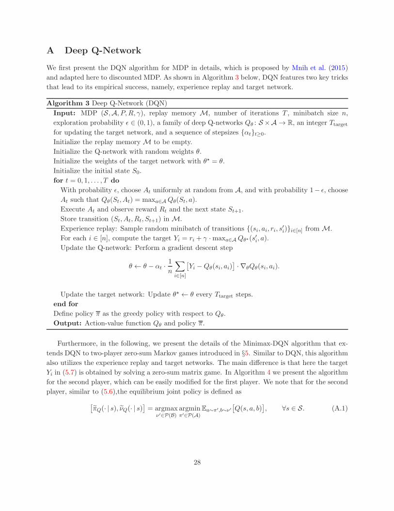
A Deep Q-Network

We first present the DQN algorithm for MDP in details, which is proposed by Mnih et al. (2015)

and adapted here to discounted MDP. As shown in Algorithm 3 below, DQN features two key tricks

that lead to its empirical success, namely, experience replay and target network.

Algorithm 3 Deep Q-Network (DQN)

Input: MDP (S,A, P,R, γ), replay memory M, number of iterations T , minibatch size n,

exploration probability ǫ ∈ (0, 1), a family of deep Q-networks Qθ : S ×A → R, an integer Ttargetfor updating the target network, and a sequence of stepsizes {αt}t≥0.

Initialize the replay memoryM to be empty.

Initialize the Q-network with random weights θ.

Initialize the weights of the target network with θ⋆ = θ.

Initialize the initial state S0.

for t = 0, 1, . . . , T do

With probability ǫ, choose At uniformly at random from A, and with probability 1− ǫ, chooseAt such that Qθ(St, At) = maxa∈AQθ(St, a).Execute At and observe reward Rt and the next state St+1.

Store transition (St, At, Rt, St+1) inM.

Experience replay: Sample random minibatch of transitions {(si, ai, ri, s′i)}i∈[n] fromM.

For each i ∈ [n], compute the target Yi = ri + γ ·maxa∈AQθ⋆(s′i, a).Update the Q-network: Perform a gradient descent step

θ ← θ − αt ·1

n

∑

i∈[n]

[Yi −Qθ(si, ai)

]· ∇θQθ(si, ai).

Update the target network: Update θ⋆ ← θ every Ttarget steps.

end for

Define policy π as the greedy policy with respect to Qθ.

Output: Action-value function Qθ and policy π.

Furthermore, in the following, we present the details of the Minimax-DQN algorithm that ex-

tends DQN to two-player zero-sum Markov games introduced in §5. Similar to DQN, this algorithm

also utilizes the experience replay and target networks. The main difference is that here the target

Yi in (5.7) is obtained by solving a zero-sum matrix game. In Algorithm 4 we present the algorithm

for the second player, which can be easily modified for the first player. We note that for the second

player, similar to (5.6),the equilibrium joint policy is defined as

[πQ(· | s), νQ(· | s)

]= argmax

ν′∈P(B)argminπ′∈P(A)

Ea∼π′,b∼ν′[Q(s, a, b)

], ∀s ∈ S. (A.1)

28

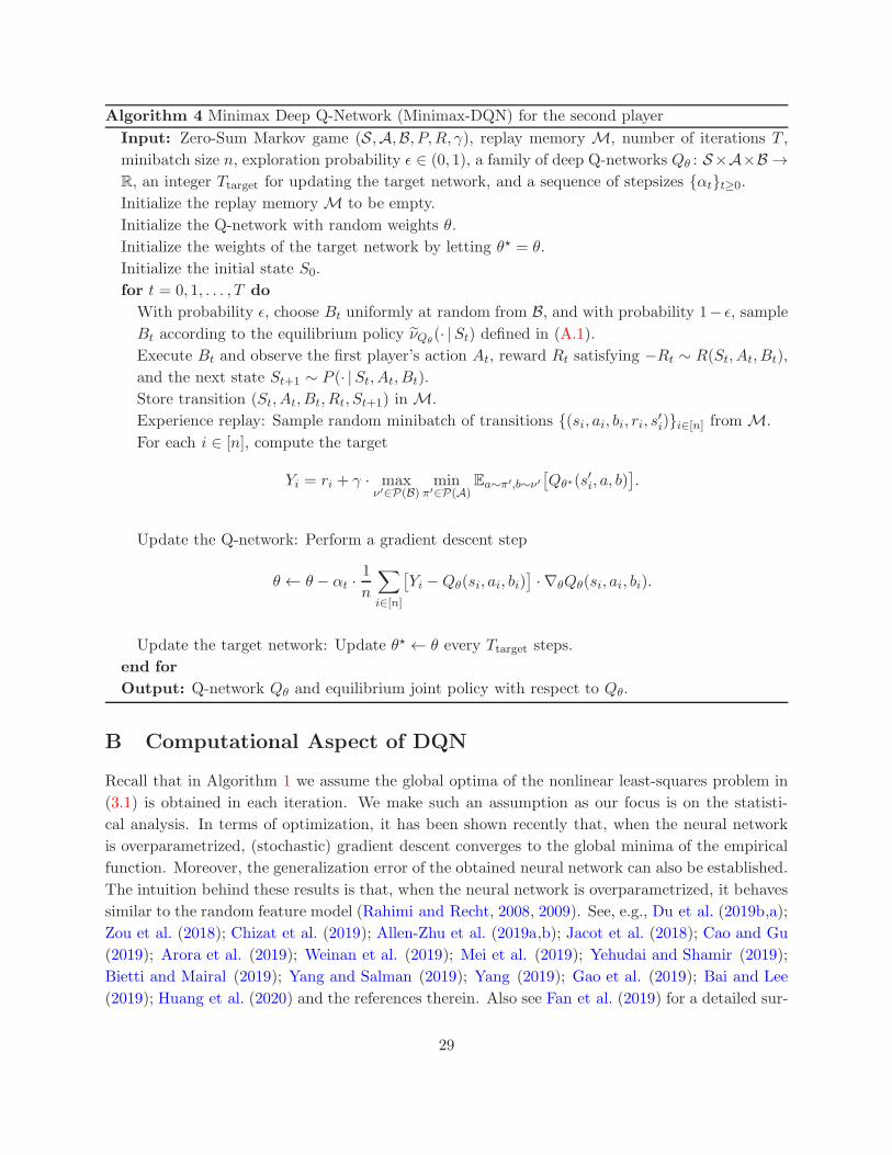
Algorithm 4 Minimax Deep Q-Network (Minimax-DQN) for the second player

Input: Zero-Sum Markov game (S,A,B, P,R, γ), replay memory M, number of iterations T ,

minibatch size n, exploration probability ǫ ∈ (0, 1), a family of deep Q-networks Qθ : S×A×B →R, an integer Ttarget for updating the target network, and a sequence of stepsizes {αt}t≥0.

Initialize the replay memoryM to be empty.

Initialize the Q-network with random weights θ.

Initialize the weights of the target network by letting θ⋆ = θ.

Initialize the initial state S0.

for t = 0, 1, . . . , T do

With probability ǫ, choose Bt uniformly at random from B, and with probability 1− ǫ, sample

Bt according to the equilibrium policy νQθ(· |St) defined in (A.1).

Execute Bt and observe the first player’s action At, reward Rt satisfying −Rt ∼ R(St, At, Bt),and the next state St+1 ∼ P (· |St, At, Bt).Store transition (St, At, Bt, Rt, St+1) inM.

Experience replay: Sample random minibatch of transitions {(si, ai, bi, ri, s′i)}i∈[n] fromM.

For each i ∈ [n], compute the target

Yi = ri + γ · maxν′∈P(B)

minπ′∈P(A)

Ea∼π′,b∼ν′[Qθ∗(s

′i, a, b)

].

Update the Q-network: Perform a gradient descent step

θ ← θ − αt ·1

n

∑

i∈[n]

[Yi −Qθ(si, ai, bi)

]· ∇θQθ(si, ai, bi).

Update the target network: Update θ⋆ ← θ every Ttarget steps.

end for

Output: Q-network Qθ and equilibrium joint policy with respect to Qθ.

B Computational Aspect of DQN

Recall that in Algorithm 1 we assume the global optima of the nonlinear least-squares problem in

(3.1) is obtained in each iteration. We make such an assumption as our focus is on the statisti-

cal analysis. In terms of optimization, it has been shown recently that, when the neural network

is overparametrized, (stochastic) gradient descent converges to the global minima of the empirical

function. Moreover, the generalization error of the obtained neural network can also be established.

The intuition behind these results is that, when the neural network is overparametrized, it behaves

similar to the random feature model (Rahimi and Recht, 2008, 2009). See, e.g., Du et al. (2019b,a);

Zou et al. (2018); Chizat et al. (2019); Allen-Zhu et al. (2019a,b); Jacot et al. (2018); Cao and Gu

(2019); Arora et al. (2019); Weinan et al. (2019); Mei et al. (2019); Yehudai and Shamir (2019);

Bietti and Mairal (2019); Yang and Salman (2019); Yang (2019); Gao et al. (2019); Bai and Lee

(2019); Huang et al. (2020) and the references therein. Also see Fan et al. (2019) for a detailed sur-

29

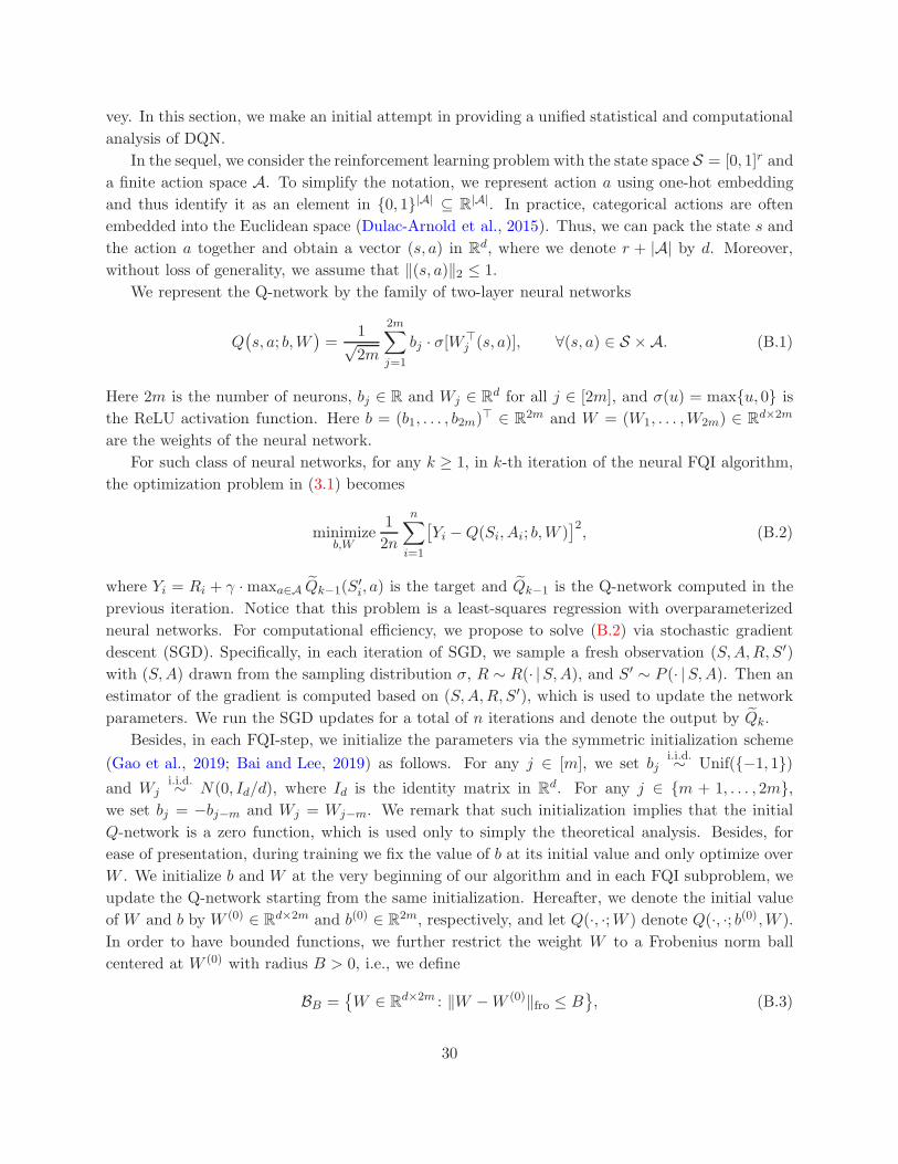
vey. In this section, we make an initial attempt in providing a unified statistical and computational

analysis of DQN.

In the sequel, we consider the reinforcement learning problem with the state space S = [0, 1]r and

a finite action space A. To simplify the notation, we represent action a using one-hot embedding

and thus identify it as an element in {0, 1}|A| ⊆ R|A|. In practice, categorical actions are often

embedded into the Euclidean space (Dulac-Arnold et al., 2015). Thus, we can pack the state s and

the action a together and obtain a vector (s, a) in Rd, where we denote r + |A| by d. Moreover,

without loss of generality, we assume that ‖(s, a)‖2 ≤ 1.

We represent the Q-network by the family of two-layer neural networks

Q(s, a; b,W

)=

1√2m

2m∑

j=1

bj · σ[W⊤j (s, a)], ∀(s, a) ∈ S ×A. (B.1)

Here 2m is the number of neurons, bj ∈ R and Wj ∈ Rd for all j ∈ [2m], and σ(u) = max{u, 0} is

the ReLU activation function. Here b = (b1, . . . , b2m)⊤ ∈ R

2m and W = (W1, . . . ,W2m) ∈ Rd×2m

are the weights of the neural network.

For such class of neural networks, for any k ≥ 1, in k-th iteration of the neural FQI algorithm,

the optimization problem in (3.1) becomes

minimizeb,W

1

2n

n∑

i=1

[Yi −Q(Si, Ai; b,W )

]2, (B.2)

where Yi = Ri + γ ·maxa∈A Qk−1(S′i, a) is the target and Qk−1 is the Q-network computed in the

previous iteration. Notice that this problem is a least-squares regression with overparameterized

neural networks. For computational efficiency, we propose to solve (B.2) via stochastic gradient

descent (SGD). Specifically, in each iteration of SGD, we sample a fresh observation (S,A,R, S′)with (S,A) drawn from the sampling distribution σ, R ∼ R(· |S,A), and S′ ∼ P (· |S,A). Then an

estimator of the gradient is computed based on (S,A,R, S′), which is used to update the network

parameters. We run the SGD updates for a total of n iterations and denote the output by Qk.

Besides, in each FQI-step, we initialize the parameters via the symmetric initialization scheme

(Gao et al., 2019; Bai and Lee, 2019) as follows. For any j ∈ [m], we set bji.i.d.∼ Unif({−1, 1})

and Wji.i.d.∼ N(0, Id/d), where Id is the identity matrix in R

d. For any j ∈ {m + 1, . . . , 2m},we set bj = −bj−m and Wj = Wj−m. We remark that such initialization implies that the initial

Q-network is a zero function, which is used only to simply the theoretical analysis. Besides, for

ease of presentation, during training we fix the value of b at its initial value and only optimize over

W . We initialize b and W at the very beginning of our algorithm and in each FQI subproblem, we

update the Q-network starting from the same initialization. Hereafter, we denote the initial value

of W and b by W (0) ∈ Rd×2m and b(0) ∈ R

2m, respectively, and let Q(·, ·;W ) denote Q(·, ·; b(0),W ).

In order to have bounded functions, we further restrict the weight W to a Frobenius norm ball

centered at W (0) with radius B > 0, i.e., we define

BB ={W ∈ R

d×2m : ‖W −W (0)‖fro ≤ B}, (B.3)

30

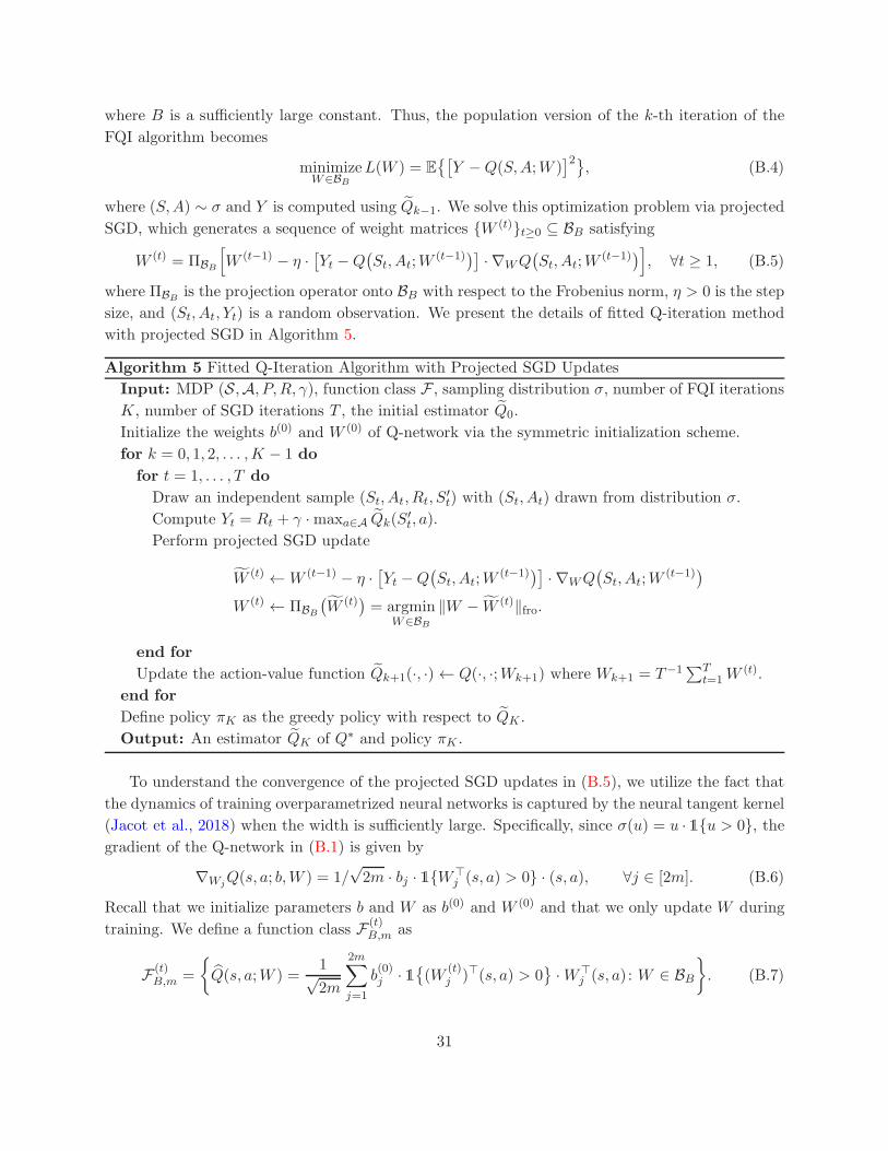
where B is a sufficiently large constant. Thus, the population version of the k-th iteration of the

FQI algorithm becomes

minimizeW∈BB

L(W ) = E{[Y −Q(S,A;W )

]2}, (B.4)

where (S,A) ∼ σ and Y is computed using Qk−1. We solve this optimization problem via projected

SGD, which generates a sequence of weight matrices {W (t)}t≥0 ⊆ BB satisfying

W (t) = ΠBB

[W (t−1) − η ·

[Yt −Q

(St, At;W

(t−1))]· ∇WQ

(St, At;W

(t−1))], ∀t ≥ 1, (B.5)

where ΠBBis the projection operator onto BB with respect to the Frobenius norm, η > 0 is the step

size, and (St, At, Yt) is a random observation. We present the details of fitted Q-iteration method

with projected SGD in Algorithm 5.

Algorithm 5 Fitted Q-Iteration Algorithm with Projected SGD Updates

Input: MDP (S,A, P,R, γ), function class F , sampling distribution σ, number of FQI iterations

K, number of SGD iterations T , the initial estimator Q0.

Initialize the weights b(0) and W (0) of Q-network via the symmetric initialization scheme.

for k = 0, 1, 2, . . . ,K − 1 do

for t = 1, . . . , T do

Draw an independent sample (St, At, Rt, S′t) with (St, At) drawn from distribution σ.

Compute Yt = Rt + γ ·maxa∈A Qk(S′t, a).

Perform projected SGD update

W (t) ←W (t−1) − η ·[Yt −Q

(St, At;W

(t−1))]· ∇WQ

(St, At;W

(t−1))

W (t) ← ΠBB

(W (t)

)= argmin

W∈BB

‖W − W (t)‖fro.

end for

Update the action-value function Qk+1(·, ·)← Q(·, ·;Wk+1) where Wk+1 = T−1∑T

t=1W(t).

end for

Define policy πK as the greedy policy with respect to QK .

Output: An estimator QK of Q∗ and policy πK .

To understand the convergence of the projected SGD updates in (B.5), we utilize the fact that

the dynamics of training overparametrized neural networks is captured by the neural tangent kernel

(Jacot et al., 2018) when the width is sufficiently large. Specifically, since σ(u) = u · 1{u > 0}, thegradient of the Q-network in (B.1) is given by

∇WjQ(s, a; b,W ) = 1/

√2m · bj · 1{W⊤

j (s, a) > 0} · (s, a), ∀j ∈ [2m]. (B.6)

Recall that we initialize parameters b and W as b(0) and W (0) and that we only update W during

training. We define a function class F (t)B,m as

F (t)B,m =

{Q(s, a;W ) =

1√2m

2m∑

j=1

b(0)j · 1

{(W

(t)j )⊤(s, a) > 0

}·W⊤

j (s, a) : W ∈ BB}. (B.7)

31

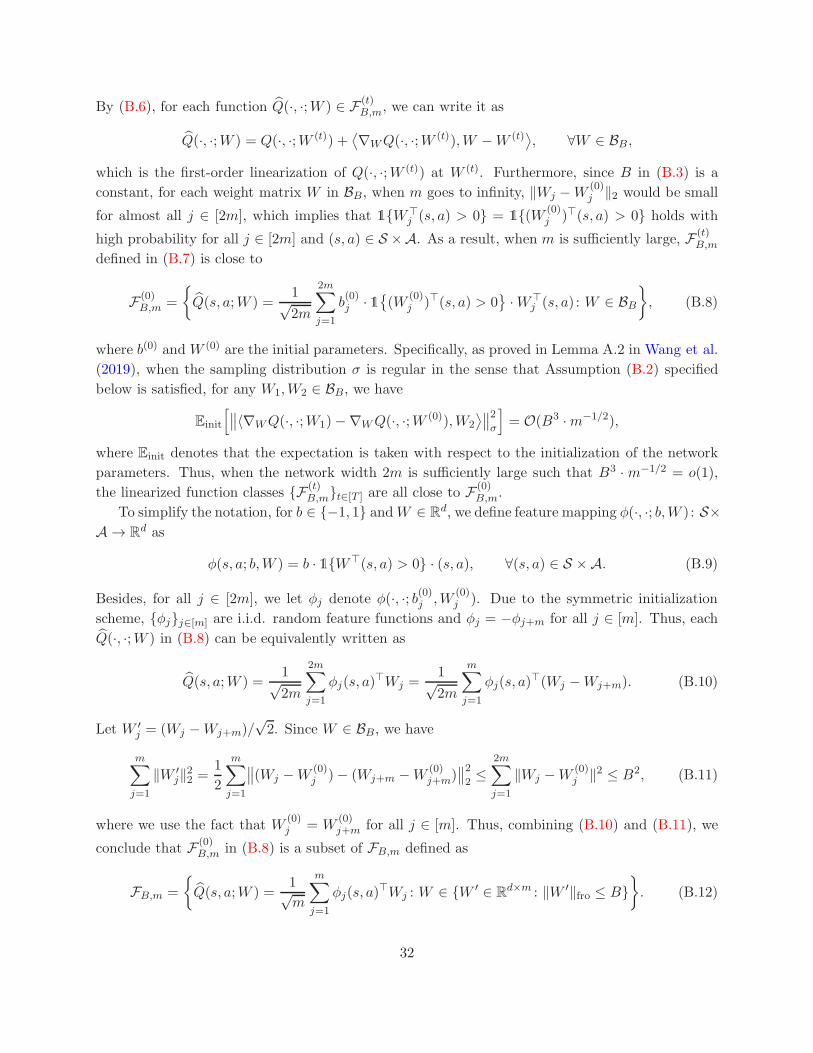
By (B.6), for each function Q(·, ·;W ) ∈ F (t)B,m, we can write it as

Q(·, ·;W ) = Q(·, ·;W (t)) +⟨∇WQ(·, ·;W (t)),W −W (t)

⟩, ∀W ∈ BB ,

which is the first-order linearization of Q(·, ·;W (t)) at W (t). Furthermore, since B in (B.3) is a

constant, for each weight matrix W in BB, when m goes to infinity, ‖Wj −W (0)j ‖2 would be small

for almost all j ∈ [2m], which implies that 1{W⊤j (s, a) > 0} = 1{(W (0)

j )⊤(s, a) > 0} holds with

high probability for all j ∈ [2m] and (s, a) ∈ S ×A. As a result, when m is sufficiently large, F (t)B,m

defined in (B.7) is close to

F (0)B,m =

{Q(s, a;W ) =

1√2m

2m∑

j=1

b(0)j · 1

{(W

(0)j )⊤(s, a) > 0

}·W⊤

j (s, a) : W ∈ BB}, (B.8)

where b(0) andW (0) are the initial parameters. Specifically, as proved in Lemma A.2 in Wang et al.

(2019), when the sampling distribution σ is regular in the sense that Assumption (B.2) specified

below is satisfied, for any W1,W2 ∈ BB, we have

Einit

[∥∥〈∇WQ(·, ·;W1)−∇WQ(·, ·;W (0)),W2

⟩∥∥2σ

]= O(B3 ·m−1/2),

where Einit denotes that the expectation is taken with respect to the initialization of the network

parameters. Thus, when the network width 2m is sufficiently large such that B3 ·m−1/2 = o(1),

the linearized function classes {F (t)B,m}t∈[T ] are all close to F (0)

B,m.

To simplify the notation, for b ∈ {−1, 1} andW ∈ Rd, we define feature mapping φ(·, ·; b,W ) : S×

A → Rd as

φ(s, a; b,W ) = b · 1{W⊤(s, a) > 0} · (s, a), ∀(s, a) ∈ S ×A. (B.9)

Besides, for all j ∈ [2m], we let φj denote φ(·, ·; b(0)j ,W(0)j ). Due to the symmetric initialization

scheme, {φj}j∈[m] are i.i.d. random feature functions and φj = −φj+m for all j ∈ [m]. Thus, each

Q(·, ·;W ) in (B.8) can be equivalently written as

Q(s, a;W ) =1√2m

2m∑

j=1

φj(s, a)⊤Wj =

1√2m

m∑

j=1

φj(s, a)⊤(Wj −Wj+m). (B.10)

Let W ′j = (Wj −Wj+m)/

√2. Since W ∈ BB, we have

m∑

j=1

‖W ′j‖22 =

1

2

m∑

j=1

∥∥(Wj −W (0)j )− (Wj+m −W (0)

j+m)∥∥22≤

2m∑

j=1

‖Wj −W (0)j ‖2 ≤ B2, (B.11)

where we use the fact that W(0)j = W

(0)j+m for all j ∈ [m]. Thus, combining (B.10) and (B.11), we

conclude that F (0)B,m in (B.8) is a subset of FB,m defined as

FB,m =

{Q(s, a;W ) =

1√m

m∑

j=1

φj(s, a)⊤Wj : W ∈ {W ′ ∈ R

d×m : ‖W ′‖fro ≤ B}}. (B.12)

32

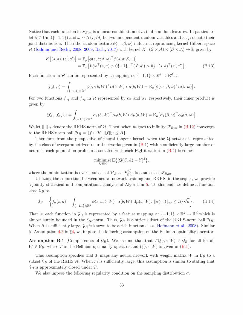
Notice that each function in FB,m is a linear combination of m i.i.d. random features. In particular,

let β ∈ Unif({−1, 1}) and ω ∼ N(Id/d) be two independent random variables and let µ denote their

joint distribution. Then the random feature φ(·, ·;β, ω) induces a reproducing kernel Hilbert space

H (Rahimi and Recht, 2008, 2009; Bach, 2017) with kernel K : (S × A)× (S × A)→ R given by

K[(s, a), (s′, a′)

]= Eµ

[φ(s, a;β, ω)⊤φ(s, a;β, ω)

]

= Eω

[1{ω⊤(s, a) > 0} · 1{ω⊤(s′, a′) > 0} · (s, a)⊤(s′, a′)

]. (B.13)

Each function in H can be represented by a mapping α : {−1, 1} × Rd → R

d as

fα(·, ·) =∫

{−1,1}×Rd

φ(·, ·; b,W )⊤α(b,W ) dµ(b,W ) = Eµ

[φ(·, ·;β, ω)⊤α(β, ω)

].

For two functions fα1and fα2

in H represented by α1 and α2, respectively, their inner product is

given by

〈fα1, fα2〉H =

∫

{−1,1}×Rd

α1(b,W )⊤α2(b,W ) dµ(b,W ) = Eµ

[α1(β, ω)

⊤α2(β, ω)].

We let ‖·‖H denote the RKHS norm of H. Then, when m goes to infinity, FB,m in (B.12) converges

to the RKHS norm ball HB = {f ∈ H : ‖f‖H ≤ B}.Therefore, from the perspective of neural tangent kernel, when the Q-network is represented

by the class of overparametrized neural networks given in (B.1) with a sufficiently large number of

neurons, each population problem associated with each FQI iteration in (B.4) becomes

minimizeQ∈H

E{[Q(S,A) − Y ]2

},

where the minimization is over a subset of HB as F (0)B,m is a subset of FB,m.

Utilizing the connection between neural network training and RKHS, in the sequel, we provide

a jointly statistical and computational analysis of Algorithm 5. To this end, we define a function

class GB as

GB =

{fα(s, a) =

∫

{−1,1}×Rd

φ(s, a; b,W )⊤α(b,W ) dµ(b,W ) : ‖α(·, ·)‖∞ ≤ B/√d

}. (B.14)

That is, each function in GB is represented by a feature mapping α : {−1, 1} × Rd → R

d which is

almost surely bounded in the ℓ∞-norm. Thus, GB is a strict subset of the RKHS-norm ball HB .When B is sufficiently large, GB is known to be a rich function class (Hofmann et al., 2008). Similar

to Assumption 4.2 in §4, we impose the following assumption on the Bellman optimality operator.

Assumption B.1 (Completeness of GB). We assume that that TQ(·, ·;W ) ∈ GB for all for all

W ∈ BB, where T is the Bellman optimality operator and Q(·, ·;W ) is given in (B.1).

This assumption specifies that T maps any neural network with weight matrix W in BB to a

subset GB of the RKHS H. When m is sufficiently large, this assumption is similar to stating that

GB is approximately closed under T .

We also impose the following regularity condition on the sampling distribution σ.

33

Assumption B.2 (Regularity Condition on σ). We assume that there exists an absolute constant

C > 0 such that

Eσ

[1{|y⊤(S,A)| ≤ u

}]≤ C · u/‖y‖2, ∀y ∈ R

d, ∀u > 0.

Assumption B.2 states that the density of σ is sufficiently regular, which holds when the density

is upper bounded.

Now we are ready to present the main result of this section, which characterizes the performance

of πK returned by Algorithm 5.

Theorem B.3. In Algorithm 5, we assume that each step of the fitted-Q iteration is solved by T

steps of projected SGD updates with a constant stepsize η > 0. We set T = C1m and η = C2/√T ,

where C1, C2 are absolute constants that are properly chosen. Then, under Assumptions 4.3, B.1,

and B.2, we have

Einit

[‖Q∗ −QπK‖1,µ

]= O

(φµ,σγ

(1− γ)2 · (B3/2 ·m−1/4 +B5/4 ·m−1/8) +

γK+1

(1− γ)2 · Rmax

), (B.15)

where Einit denotes that the expectation is taken with respect to the randomness of the initialization.

As shown in (B.15), the error Einit[‖Q∗ − QπK‖1,µ] can be similarly written as the sum of a

statistical error and an algorithmic error, where the algorithmic error converges to zero at a linear

rate as K goes to infinity. The statistical error corresponds to the error incurred in solving each

FQI step via T projected SGD steps. As shown in (B.15), when B is regarded as a constant, with

T ≍ m projected SGD steps, we obtain an estimator with error O(m−1/8). Hence, Algorithm

5 finds the globally optimal policy when both m and K goes to infinity. Therefore, when using

overparametrized neural networks, our fitted Q-iteration algorithm provably attains both statistical

accuracy and computational efficiency.

Finally, we remark that focus on the class of two-layer overparametrized ReLU neural networks

only for the simplicity of presentation. The theory of neural tangent kernel can be extended

to feedforward neural networks with multiple layers and neural networks with more complicated

architectures (Gao et al., 2019; Frei et al., 2019; Yang and Salman, 2019; Yang, 2019; Huang et al.,

2020).

B.1 Proof of Theorem B.3

Proof. Our proof is similar to that of Theorem 4.4. For any k ∈ [K], we define the maximum

one-step approximation error as εmax = maxk∈[K]Einit[‖TQk−1 − Qk‖σ], where Einit denotes that

the expectation is taken with respect to the randomness in the initialization of network weights,

namely b(0) and W (0). By Theorem 6.1, we have

Einit

[‖Q∗ −QπK‖1,µ

]≤ 2φµ,σγ

(1− γ)2 · εmax +4γK+1

(1− γ)2 · Rmax, (B.16)

where φµ,σ , specified in Assumption 4.3, is a constant that only depends on the concentration

coefficients. Thus, it remains to characterize ‖TQk−1 − Qk‖σ for each k, which corresponds to the

prediction risk of the estimator constructed by T projected SGD steps.

34

In the sequel, we characterize the prediction risk of the projected SGDmethod via the framework

of neural tangent kernel. Our proof technique is motivated by recent work (Gao et al., 2019;

Cai et al., 2019; Liu et al., 2019a; Wang et al., 2019; Xu and Gu, 2019) which analyze the training

of overparametrized neural networks via projected SGD for adversarial training and reinforcement

learning. We focus on the case where the target network is Qk−1 and bound ‖TQk−1 − Qk‖σ .To begin with, recall that we define function classes F (t)

B,m, FB,m, and GB in (B.7), (B.12), and

(B.14), respectively. Notice that Qk−1 = Q(·, ·;Wk) is a neural network where Wk ∈ BB due to

projection. Then, by Assumption B.1, TQk−1 belongs to GB , which is a subset of the RKHS H.Thus, it suffices to study the least-squares regression problem where the target function is in GBand the neural network is trained via projected SGD.

In the following, we use function class FB,m to connect GB and Qk. Specifically, we show that

any function g ∈ GB as well as Qk can be well approximated by functions in FB,m and quantify

the approximation errors. Finally, we focus on the projected SGD algorithm within the linearized

function class FB,m and establish the statistical and computational error. The proof is divided into

three steps as follows.

Step (i). In the first step, we quantify the difference between Qk and functions in FB,m. For anyj ∈ [2m], let [Wk+1]j ∈ R

d be the weights of Qk corresponding to the j-th neuron. We define a

function Qk : S × A → R as Qk(s, a) = 1/√2m ·∑2m

j=1 φj(s, a)⊤[Wk+1]j , which belongs to F (0)

B,m

defined in (B.8), a subset of FB,m. The following following lemma, obtained from Wang et al.

(2019), prove that Q(·, ·;W ) is close to a linearized function when m is sufficiently large.

Lemma B.4 (Linearization Error). Let BB be defined in (B.3). Under Assumption B.2, for any

W (1),W (2) ∈ BB, we have

Einit

[∥∥〈∇WQ(·, ·;W (1))−∇WQ(·, ·;W (0)),W (2)⟩∥∥2

σ

]= O(B3 ·m−1/2).

Proof. See Lemma A.2 in Wang et al. (2019) for a detailed proof.

Notice that we have Qk(·, ·) = 〈∇WQ(·, ·;Wk+1),Wk+1〉 and Qk(·, ·) = 〈∇WQ(·, ·;W (0)),Wk+1〉.Applying Lemma B.4 with W (1) =W (2) =Wk+1, we obtain that

Einit

[∥∥Qk − Qk∥∥2σ

]= Einit

[Eσ

{[Qk(S,A)− Qk(S,A)]2

}]= O(B3 ·m−1/2). (B.17)

Thus, we have constructed a function in FB,m that is close to Qk whenm is sufficiently large, which

completes the first step of the proof.

Step (2). In the second step, we show that each function in GB can also be well approximated by

functions in FB,m. To this end, similar to the definition of GB in (B.14), we define a function class

FB,m as

FB,m =

{Q(s, a;W ) =

1√m·m∑

j=1

φj(s, a)⊤Wj : ‖Wj‖∞ ≤ B/

√md

}, (B.18)

35

which is a subset of FB,m by definition. Intuitively, as m goes to infinity, FB,m becomes GB. Thefollowing Lemma, obtained from (Rahimi and Recht, 2009), provides a rigorous characterization of

this argument.

Lemma B.5 (Approximation Error of FB,m (Rahimi and Recht, 2009)). Let Q be any fixed func-

tion in GB and define ΠB,mQ ∈ FR,m as the solution to

minimizef∈FB,m

‖f −Q‖σ.

Then, there exists a constant C > 0 such that, for any t > B/√m, we have

Pinit

(∥∥ΠB,mQ−Q∥∥σ> t

)≤ C · exp

[−1/2 · (t · √m/B − 1)2

]. (B.19)

Proof. See Rahimi and Recht (2009) for a detailed proof.

Now we integrate the tail probability in (B.19) to obtain a bound on Einit[‖ΠB,mQ − Q‖σ].Specifically, by direct computation, we have

Einit

[∥∥ΠB,mQ−Q∥∥2σ

]=

∫ ∞

02t · Pinit

(∥∥ΠB,mQ−Q∥∥2σ> t2

)dt

≤ 2B2/m+ 2C ·∫ ∞

B/√mt · exp

[−1/2 · (t · √m/B − 1)2

]dt

= B2/√m+ C ·B2/m ·

∫ ∞

0(1 + u) · exp(−1/2 · u2) du = O(B2 ·m−1), (B.20)

where in the second equality we let u = t · √m/B − 1. Thus, by (B.20) we have

Einit

[∥∥T Qk−1 − TQk−1

∥∥2σ

]= O(B2 ·m−1), (B.21)

where T Qk−1 = ΠB,mTQk−1. Thus, we conclude the second step.

Step (3). Finally, in the last step, we utilize the existing analysis of projected SGD over function

class FB,m to obtain an upper bound on ‖T Qk−1 − Qk‖.

Theorem B.6 (Convergence of Projected SGD (Liu et al., 2019a)). In Algorithm 5, let T be the

number of iterations of projected SGD steps for solving each iteration of the FQI update and we

set η = O(1/√T ). Under Assumption B.2, it holds that

Einit

[∥∥Qk − T Qk−1

∥∥2σ

]≤ O(B2 · T−1/2 +B3 ·m−1/2 +B5/2 ·m−1/4). (B.22)

Proof. See Theorem 4.5 in Liu et al. (2019a) for a detailed proof.

Finally, combining (B.17), (B.21), and (B.22) we obtain that

Einit

[∥∥Qk − TQk−1

∥∥2σ

]

≤ 3Einit

[∥∥Qk − Qk∥∥2σ

]+ 3Einit

[∥∥T Qk−1 − TQk−1

∥∥2σ

]+ 3Einit

[∥∥Qk − T Qk−1

∥∥2σ

]

= O(B2 · T−1/2 +B2 ·m−1 +B3 ·m−1/2 +B5/2 ·m−1/4

). (B.23)

36

Setting T ≍ m in (B.23), we obtain that

εmax = maxk∈[K]

Einit

[∥∥TQk−1 − Qk∥∥σ

]≤ O(B3/2 ·m−1/4 +B5/4 ·m−1/8). (B.24)

Combining (B.16) and (B.24), we conclude the proof of Theorem B.3.

C Proofs of Auxiliary Results

In this section, we present the proofs for Theorems 6.1 and 6.2, which are used in the §6 to establish

our main theorem.

C.1 Proof of Theorem 6.1

Proof. Before we present the proof, we introduce some notation. For any k ∈ {0, . . . ,K − 1}, wedenote TQk by Qk+1 and define

k = Qk − Qk. (C.1)

Also, we denote by πk the greedy policy with respect to Qk. In addition, throughout the proof,

for two functions Q1, Q2 : S × A → R, we use the notation Q1 ≥ Q2 if Q1(s, a) ≥ Q2(s, a) for any

s ∈ S and any a ∈ A, and define Q1 ≤ Q2 similarly. Furthermore, for any policy π, recall that in

(2.4) we define the operator P π by

(P πQ)(s, a) = E[Q(S′, A′)

∣∣S′ ∼ P (· | s, a), A′ ∼ π(· |S′)]. (C.2)

In addition, we define the operator T π by

(T πQ)(s, a) = r(s, a) + γ · (P πQ)(s, a).

Finally, we denote Rmax/(1 − γ) by Vmax. Now we are ready to present the proof, which consists

of three key steps.

Step (i): In the first step, we establish a recursion that relates Q∗−Qk+1 with Q∗−Qk to measure

the sub-optimality of the value function Qk. In the following, we first establish an upper bound for

Q∗ − Qk+1 as follows. For each k ∈ {0, . . . ,K − 1}, by the definition of k+1 in (C.1), we have

Q∗ − Qk+1 = Q∗ − (Qk+1 − k+1) = Q∗ −Qk+1 + k+1 = Q∗ − TQk + k+1

= Q∗ − T π∗

Qk + (T π∗

Qk − TQk) + k+1, (C.3)

where π∗ is the greedy policy with respect to Q∗. Now we leverage the following lemma to show

T π∗Qk ≤ TQk.

Lemma C.1. For any action-value function Q : S × A → R and any policy π, it holds that

T πQQ = TQ ≥ T πQ.

37

Proof. Note that we have maxa′ Q(s′, a′) ≥ Q(s′, a′) for any s′ ∈ S and a′ ∈ A. Thus, it holds that

(TQ)(s, a) = r(s, a) + γ · E[maxa′

Q(S′, a′)∣∣S′ ∼ P (· | s, a)

]

≥ r(s, a) + γ · E[Q(S′, A′)

∣∣S′ ∼ P (· | s, a), A′ ∼ π(· |S′)]= (T πQ)(s, a).

Recall that πQ is the greedy policy with respect to Q such that

P[A ∈ argmax

aQ(s, a)

∣∣A ∼ πQ(· | s)]= 1,

which implies

E[Q(s′, A′)

∣∣A′ ∼ πQ(· | s′)]= max

a′Q(s′, a′).

Consequently, we have

(T πQQ)(s, a) = r(s, a) + γ · E[Q(S′, A′)

∣∣S′ ∼ P (· | s, a), A′ ∼ πQ(· |S′)]

= r(s, a) + γ · E[maxa′

Q(S′, a′)∣∣S′ ∼ P (· | s, a)

]= (TQ)(s, a),

which concludes the proof of Lemma C.1.

By Lemma C.1, we have TQk ≥ T π∗Qk. Also note that Q∗ is the unique fixed point of T π

∗.

Thus, by (C.3) we have

Q∗ − Qk+1 = (T π∗

Q∗ − T π∗

Qk) + (T π∗

Qk − TQk) + k+1 ≤ (T π∗

Q∗ − T π∗

Qk) + k+1, (C.4)

In the following, we establish a lower bound for Q∗−Qk+1 based on Q∗−Qk. Note that, by Lemma

C.1, we have T πkQk = TQk and TQ∗ ≥ T πkQ∗. Similar to (C.3), since Q∗ is the unique fixed point

of T , it holds that

Q∗ − Qk+1 = Q∗ − TQk + k+1 = Q∗ − T πkQk + k+1 = Q∗ − T πkQ∗ + (T πkQ∗ − T πkQk) + k+1

= (TQ∗ − T πkQ∗) + (T πkQ∗ − T πkQk) + k+1 ≥ (T πkQ∗ − T πkQk) + k+1. (C.5)

Thus, combining (C.4) and (C.5) we obtain that, for any k ∈ {0, . . . ,K − 1},

T πkQ∗ − T πkQk + k+1 ≤ Q∗ − Qk+1 ≤ T π∗

Q∗ − T π∗

Qk + k+1. (C.6)

The inequalities in (C.6) show that the error Q∗− Qk+1 can be sandwiched by the summation of a

term involving Q∗− Qk and the error k+1, which is defined in (C.1) and induced by approximating

the action-value function. Using P π defined in (C.2), we can write (C.6) in a more compact form,

γ · P π∗

(Q∗ − Qk) + k+1 ≥ Q∗ − Qk+1 ≥ γ · P πk(Q∗ − Qk) + k+1. (C.7)

Meanwhile, note that P π defined in (C.2) is a linear operator. In fact, P π is the Markov transition

operator for the Markov chain on S × A with transition dynamics

St+1 ∼ P (· |St, At), At+1 ∼ π(· | St+1).

By the linearity of the operator P π and the one-step error bound in (C.6), we have the following

characterization of the multi-step error.

38

Lemma C.2 (Error Propagation). For any k, ℓ ∈ {0, 1, . . . ,K − 1} with k < ℓ, we have

Q∗ − Qℓ ≤ℓ−1∑

i=k

γℓ−1−i · (P π∗

)ℓ−1−ii+1 + γℓ−k · (P π∗

)ℓ−k(Q∗ − Qk), (C.8)

Q∗ − Qℓ ≥ℓ−1∑

i=k

γℓ−1−i · (P πℓ−1P πℓ−2 · · ·P πi+1)i+1 + γℓ−k · (P πℓ−1P πℓ−2 · · ·P πk)(Q∗ − Qk). (C.9)

Here i+1 is defined in (C.1) and we use P πP π′and (P π)k to denote the composition of operators.

Proof. Note that P π is a linear operator for any policy π. We obtain (C.8) and (C.9) by iteratively

applying the inequalities in (C.7).

Lemma C.2 gives the upper and lower bounds for the propagation of error through multiple

iterations of Algorithm 1, which concludes the first step of our proof.

Step (ii): The results in the first step only concern the propagation of error Q∗− Qk. In contrast,

the output of Algorithm 1 is the greedy policy πk with respect to Qk. In the second step, our goal

is to quantify the suboptimality of Qπk , which is the action-value function corresponding to πk. In

the following, we establish an upper bound for Q∗ −Qπk .To begin with, we have Q∗ ≥ Qπk by the definition ofQ∗ in (2.5). Note that we have Q∗ = T π

∗Q∗

and Qπk = T πkQπk . Hence, it holds that

Q∗ −Qπk = T π∗

Q∗ − T πkQπk = T π∗

Q∗ + (−T π∗

Qk + T π∗

Qk) + (−T πkQk + T πkQk)− T πkQπk

= (T π∗

Qk − T πkQk) + (T π∗

Q∗ − T π∗

Qk) + (T πkQk − T πkQπk). (C.10)

Now we quantify the three terms on the right-hand side of (C.10) respectively. First, by Lemma

C.1, we have

T π∗

Qk − T πkQk = T π∗

Qk − TQk ≤ 0. (C.11)

Meanwhile, by the definition of the operator P π in (C.2), we have

T π∗

Q∗ − T π∗

Qk = γ · P π∗

(Q∗ − Qk), T πkQk − T πkQπk = γ · P πk(Qk −Qπk). (C.12)

Plugging (C.11) and (C.12) into (C.10), we obtain

Q∗ −Qπk ≤ γ · P π∗

(Q∗ − Qk) + γ · P πk(Qk −Qπk)= γ · (P π∗ − P πk)(Q∗ − Qk) + γ · P πk(Q∗ −Qπk),

which further implies that

(I − γ · P πk)(Q∗ −Qπk) ≤ γ · (P π∗ − P πk)(Q∗ − Qk).

Here I is the identity operator. Since T π is a γ-contractive operator for any policy π, I − γ · P π is

invertible. Thus, we obtain

0 ≤ Q∗ −Qπk ≤ γ · (I − γ · P πk)−1[P π

∗

(Q∗ − Qk)− P πk(Q∗ − Qk)], (C.13)

39

which relates Q∗ −Qπk with Q∗ − Qk. In the following, we plug Lemma C.2 into (C.13) to obtain

the multiple-step error bounds for Qπk . First note that, by the definition of P π in (C.2), for any

functions f1, f2 : S × A → R satisfying f1 ≥ f2, we have P πf1 ≥ P πf2. Combining this inequality

with the upper bound in (C.8) and the lower bound in (C.9), we have that, for any k < ℓ,

P π∗

(Q∗ − Qℓ) ≤ℓ−1∑

i=k

γℓ−1−i · (P π∗

)ℓ−ii+1 + γℓ−k · (P π∗

)ℓ−k+1(Q∗ − Qk), (C.14)

P πℓ(Q∗ − Qℓ) ≥ℓ−1∑

i=k

γℓ−1−i · (P πℓP πℓ−1 · · ·P πi+1)i+1

+ γℓ−k · (P πℓP πℓ−1 · · ·P πk)(Q∗ − Qk). (C.15)

Then we plug (C.14) and (C.15) into (C.13) and obtain

0 ≤ Q∗ −Qπℓ ≤ (I − γ · P πℓ)−1

{ ℓ−1∑

i=k

γℓ−i ·[(P π

∗

)ℓ−i − (P πℓP πℓ−1 · · ·P πi+1)]i+1

+ γℓ+1−k ·[(P π

∗

)ℓ−k+1 − (P πℓP πℓ−1 · · ·P πk)](Q∗ − Qk)

}(C.16)

for any k < ℓ. To quantify the error of QπK , we set ℓ = K and k = 0 in (C.16) to obtain

0 ≤ Q∗ −QπK ≤ (I − γP πK )−1

{K−1∑

i=0

γK−i ·[(P π

∗

)K−i − (P πKP πK−1 · · ·P πi+1)]i+1

+ γK+1 ·[(P π

∗

)K+1 − (P πKP πK−1 · · ·P π0)](Q∗ − Q0)

}. (C.17)

For notational simplicity, we define

αi =(1− γ)γK−i−1

1− γK+1, for 0 ≤ i ≤ K − 1, and αK =

(1− γ)γK1− γK+1

. (C.18)

One can show that∑K

i=0 αi = 1. Meanwhile, we define K + 1 linear operators {Ok}Kk=0 by

Oi = (1− γ)/2 · (I − γP πK )−1[(P π

∗

)K−i + (P πKP πK−1 · · ·P πi+1)], for 0 ≤ i ≤ K − 1,

OK = (1− γ)/2 · (I − γP πK )−1[(P π

∗

)K+1 + (P πKP πK−1 · · ·P π0)].

Using this notation, for any (s, a) ∈ S ×A, by (C.17) we have

∣∣Q∗(s, a)−QπK (s, a)∣∣

≤ 2γ(1− γK+1)

(1− γ)2 ·[K−1∑

i=0

αi ·(Oi|i+1|

)(s, a) + αK ·

(OK |Q∗ − Q0|

)(s, a)

], (C.19)

where both Oi|i+1| and OK |Q∗− Q0| are functions defined on S ×A. Here (C.19) gives a uniform

upper bound for Q∗ −QπK , which concludes the second step.

40

Step (iii): In this step, we conclude the proof by establishing an upper bound for ‖Q∗ −QπK‖1,µbased on (C.19). Here µ ∈ P(S × A) is a fixed probability distribution. To simplify the notation,

for any measurable function f : S × A → R, we denote µ(f) to be the expectation of f under µ,

that is, µ(f) =∫S×A f(s, a)dµ(s, a). Using this notation, by (C.19) we bound ‖Q∗ −Qπℓ‖1,µ by

‖Q∗ −QπK‖1,µ = µ(|Q∗ −QπK |

)

≤ 2γ(1 − γK+1)

(1− γ)2 · µ[K−1∑

i=0

αi ·(Oi|i+1|

)+ αK ·

(OK |Q∗ − Q0|

)]. (C.20)

By the linearity of expectation, (C.20) implies

‖Q∗ −QπK‖1,µ ≤2γ(1 − γK+1)

(1− γ)2 ·[K−1∑

i=0

αi · µ(Oi|i+1|

)+ αK · µ

(OK |Q∗ − Q0|

)]. (C.21)

Furthermore, since both Q∗ and Q0 are bounded by Vmax = Rmax/(1 − γ) in ℓ∞-norm, we have

µ(OK |Q∗ − Q0|

)≤ 2 · Rmax/(1 − γ). (C.22)

Moreover, for any i ∈ {0, . . . ,K − 1}, by expanding (1− γP πK )−1 into a infinite series, we have

µ(Oi|i+1|

)= µ

{1− γ2· (1− γP πK )−1

[(P π

∗

)K−i + (P πKP πK−1 · · ·P πi+1)]|i+1|

}

=1− γ2· µ

{ ∞∑

j=0

γj ·[(P πK )j(P π

∗

)K−i + (P πK )j+1(P πK−1 · · ·P πi+1)]|i+1|

}. (C.23)

To upper bound the right-hand side of (C.23), we consider the following quantity

µ[(P πK )j(P τmP τm−1 · · ·P τ1)f

]=

∫

S×A

[(P πK )j(P τmP τm−1 · · ·P τ1)f

](s, a)dµ(s, a). (C.24)

Here τ1, . . . , τm arem policies. Recall that P π is the transition operator of a Markov process defined

on S × A for any policy π. Then the integral on the right-hand side of (C.24) corresponds to the

expectation of the function f(Xt), where {Xt}t≥0 is a Markov process defined on S × A. Such a

Markov process has initial distribution X0 ∼ µ. The first m transition operators are {P τj}j∈[m],

followed by j identical transition operators P πK . Hence, (P πK )j(P τmP τm−1 · · ·P τ1)µ is the marginal

distribution of Xj+m, which we denote by µj for notational simplicity. Hence, (C.24) takes the form

µ[(P πK )j(P τmP τm−1 · · ·P τ1)f

]= E

[f(Xj+m)

]= µj(f) =

∫

S×Af(s, a)dµj(s, a) (C.25)

for any measurable function f on S × A. By Cauchy-Schwarz inequality, we have

µj(f) ≤[∫

S×A

∣∣∣dµjdσ

(s, a)∣∣∣2dσ(s, a)

]1/2[∫

S×A|f(s, a)|2dσ(s, a)

]1/2, (C.26)

41

in which dµj/dσ : S × A → R is the Radon-Nikodym derivative. Recall that the (m+ j)-th order

concentration coefficient κ(m+ j;µ, σ) is defined in (4.4). Combining (C.25) and (C.26), we obtain

µj(f) ≤ κ(m+ j;µ, σ) · ‖f‖σ.Thus, by (C.23) we have

µ(Oi|i+1|

)=

1− γ2·

∞∑

j=0

γj ·{µ[(P πK )j(P π

∗

)K−i|i+1|]+ µ

[(P πK )j+1(P πK−1 · · ·P πi+1)|i+1|

]}

≤ (1− γ) ·∞∑

j=0

γj · κ(K − i+ j;µ, σ) · ‖i+1‖σ . (C.27)

Now we combine (C.21), (C.22), and (C.27) to obtain

‖Q∗ −QπK‖1,µ ≤2γ(1− γK+1)

(1− γ)2 ·[K−1∑

i=0

αi · µ(Oi|i+1|

)+ αK · µ

(OK |Q∗ − Q0|

)]

≤ 2γ(1 − γK+1)

(1− γ) ·[K−1∑

i=0

∞∑

j=0

αi · γj · κ(K − i+ j;µ, σ) · ‖i+1‖σ]+

4γ(1 − γK+1)

(1− γ)3 · αK · Rmax.

Recall that in Theorem 6.1 and (C.1) we define εmax = maxi∈[K] ‖i‖σ. We have that ‖Q∗−QπK‖1,µis further upper bounded by

‖Q∗ −QπK‖1,µ (C.28)

≤ 2γ(1 − γK+1)

(1− γ) ·[K−1∑

i=0

∞∑

j=0

αi · γj · κ(K − i+ j;µ, σ)

]· εmax +

4γ(1 − γK+1)

(1− γ)3 · αK ·Rmax

=2γ(1 − γK+1)

(1− γ) ·[K−1∑

i=0

∞∑

j=0

(1− γ)γK−i−1

1− γK+1· γj · κ(K − i+ j;µ, σ)

]· εmax +

4γK+1

(1− γ)2 ·Rmax,

where the last equality follows from the definition of {αi}0≤i≤K in (C.18). We simplify the sum-

mation on the right-hand side of (C.28) and use Assumption 4.3 to obtain

K−1∑

i=0

∞∑

j=0

(1− γ)γK−i−1

1− γK+1· γj · κ(K − i+ j;µ, σ)

=1− γ

1− γK+1

∞∑

j=0

K−1∑

i=0

γK−i+j−1 · κ(K − i+ j;µ, σ)

≤ 1− γ1− γK+1

∞∑

m=0

γm−1 ·m · κ(m;µ, σ) ≤ φµ,σ(1− γK+1)(1 − γ) , (C.29)

where the last inequality follows from (4.5) in Assumption 4.3. Finally, combining (C.28) and

(C.29), we obtain

‖Q∗ −QπK‖1,µ ≤2γ · φµ,σ(1− γ)2 · εmax +

4γK+1

(1− γ)2 ·Rmax,

which concludes the third step and hence the proof of Theorem 6.1.

42

C.2 Proof of Theorem 6.2

Proof. Recall that in Algorithm 1 we define Yi = Ri+γ ·maxa∈AQ(Si+1, a), where Q is any function

in F . By definition, we have E(Yi |Si = s,Ai = a) = (TQ)(s, a) for any (s, a) ∈ S × A. Thus,

TQ can be viewed as the underlying truth of the regression problem defined in (6.2), where the

covariates and responses are {(Si, Ai)}i∈[n] and {Yi}i∈[n], respectively. Moreover, note that TQ is

not necessarily in function class F . We denote by Q∗ the best approximation of TQ in F , which is

the solution to

minimizef∈F

‖f − TQ‖2σ = E

{[f(Si, Ai)−Q(Si, Ai)

]2}. (C.30)

For notational simplicity, in the sequel we denote (Si, Ai) by Xi for all i ∈ [n]. For any f ∈ F , wedefine ‖f‖2n = 1/n ·∑n

i=1[f(Xi)]2. Since both Q and TQ are bounded by Vmax = Rmax/(1 − γ),

we only need to consider the case where logNδ ≤ n. Here Nδ is the cardinality of N (δ,F , ‖ · ‖∞).

Moreover, let f1, . . . , fNδbe the centers of the minimal δ-covering of F . Then by the definition of

δ-covering, there exists k∗ ∈ [Nδ] such that ‖Q − fk∗‖∞ ≤ δ. It is worth mentioning that k∗ is a

random variable since Q is obtained from data.

In the following, we prove (6.3) in two steps, which are bridged by E[‖Q− TQ‖2n].Step (i): We relate E[‖Q−TQ‖2n] with its empirical counterpart ‖Q−TQ‖2n. Recall that we defineYi = Ri + γ ·maxa∈AQ(Si+1, a) for each i ∈ [n]. By the definition of Q, for any f ∈ F we have

n∑

i=1

[Yi − Q(Xi)

]2 ≤n∑

i=1

[Yi − f(Xi)

]2. (C.31)

For each i ∈ [n], we define ξi = Yi − (TQ)(Xi). Then (C.31) can be written as

‖Q− TQ‖2n ≤ ‖f − TQ‖2n +2

n

n∑

i=1

ξi ·[Q(Xi)− f(Xi)

]. (C.32)

Since both f and Q are deterministic, we have E(‖f − TQ‖2n) = ‖f − TQ‖2σ. Moreover, since

E(ξi |Xi) = 0 by definition, we have E[ξi · g(Xi)] = 0 for any bounded and measurable function g.

Thus, it holds that

E

{ n∑

i=1

ξi ·[Q(Xi)− f(Xi)

]}= E

{ n∑

i=1

ξi ·[Q(Xi)− (TQ)(Xi)

]}. (C.33)

In addition, by triangle inequality and (C.33), we have

∣∣∣∣E{ n∑

i=1

ξi ·[Q(Xi)− (TQ)(Xi)

]}∣∣∣∣

≤∣∣∣∣E

{ n∑

i=1

ξi ·[Q(Xi)− fk∗(Xi)

]}∣∣∣∣+∣∣∣∣E

{ n∑

i=1

ξi ·[fk∗(Xi)− (TQ)(Xi)

]}∣∣∣∣, (C.34)

43

where fk∗ satisfies ‖fk∗ − Q‖∞ ≤ δ. In the following, we upper bound the two terms on the right-

hand side of (C.34) respectively. For the first term, by applying Cauchy-Schwarz inequality twice,

we have∣∣∣∣E

{ n∑

i=1

ξi ·[Q(Xi)− fk∗(Xi)

]}∣∣∣∣ ≤√n ·

∣∣∣∣E[( n∑

i=1

ξ2i

)1/2

· ‖Q− fk∗‖n]∣∣∣∣

≤ √n ·[E

( n∑

i=1

ξ2i

)]1/2·[E(‖Q− fk∗‖2n

)]1/2≤ nδ ·

[E(ξ2i )

]1/2, (C.35)

where we use the fact that {ξi}i∈[n] have the same marginal distributions and ‖Q−fk∗‖n ≤ δ. Sinceboth Yi and TQ are bounded by Vmax, ξi is a bounded random variable by its definition. Thus,

there exists a constant Cξ > 0 depending on ξ such that E(ξ2i ) ≤ C2ξ · V 2

max. Then (C.35) implies

∣∣∣∣E{ n∑

i=1

ξi ·[Q(Xi)− fk∗(Xi)

]}∣∣∣∣ ≤ Cξ · Vmax · nδ. (C.36)

It remains to upper bound the second term on the right-hand side of (C.34). We first define

Nδ self-normalized random variables

Zj =1√n

n∑

i=1

ξi ·[fj(Xi)− (TQ)(Xi)

]· ‖fj − (TQ)‖−1

n (C.37)

for all j ∈ [Nδ]. Here recall that {fj}j∈[Nδ] are the centers of the minimal δ-covering of F . Then

we have∣∣∣∣E

{ n∑

i=1

ξi ·[fk∗(Xi)− (TQ)(Xi)

]}∣∣∣∣ =√n · E

[‖fk∗ − TQ‖n · |Zk∗|

]

≤ √n · E{[‖Q− TQ‖n + ‖Q− fk∗‖n

]· |Zk∗ |

}≤ √n · E

{[‖Q− TQ‖n + δ

]· |Zk∗ |

}, (C.38)

where the first inequality follows from triangle inequality and the second inequality follows from

the fact that ‖Q − fk∗‖∞ ≤ δ. Then applying Cauchy-Schwarz inequality to the last term on the

right-hand side of (C.38), we obtain

E

{[‖Q− TQ‖n + δ

]· |Zk∗ |

}≤

(E

{[‖Q− TQ‖n + δ

]2})1/2

·[E(Z2

k∗)]1/2

≤({

E[‖Q− TQ‖2n

]}1/2+ δ

)·[E(maxj∈[N ]

Z2j

)]1/2, (C.39)

where the last inequality follows from

E[‖Q− TQ‖n

]≤

{E[‖Q− TQ‖2n

]}1/2.

Moreover, since ξi is centered conditioning on {Xi}i∈[n] and is bounded by 2Vmax, ξi is a sub-

Gaussian random variable. In specific, there exists an absolute constant Hξ > 0 such that ‖ξi‖ψ2≤

Hξ · Vmax for each i ∈ [n]. Here the ψ2-norm of a random variable W ∈ R is defined as

‖W‖ψ2= sup

p≥1p−1/2

[E(|W |p)

]1/p.

44

By the definition of Zj in (C.37), conditioning on {Xi}i∈[n], ξi · [fj(Xi) − (TQ)(Xi)] is a centered

and sub-Gaussian random variable with

∥∥ξi ·[fj(Xi)− (TQ)(Xi)

]∥∥ψ2≤ Hξ · Vmax ·

∣∣fj(Xi)− (TQ)(Xi)∣∣.

Moreover, since Zj is a summation of independent sub-Gaussian random variables, by Lemma 5.9

of Vershynin (2010), the ψ2-norm of Zj satisfies

‖Zj‖ψ2≤ C ·Hξ · Vmax · ‖fj − TQ‖−1

n ·[1

n

n∑

i=1

∣∣[fj(Xi)− (TQ)(Xi)]∣∣2]1/2

≤ C ·Hξ · Vmax,

where C > 0 is an absolute constant. Furthermore, by Lemmas 5.14 and 5.15 of Vershynin (2010),

Z2j is a sub-exponential random variable, and its the moment-generating function is bounded by

E[exp(t · Z2

j )]≤ exp(C · t2 ·H4

ξ · V 4max) (C.40)

for any t satisfying C ′ · |t| · H2ξ · V 2

max ≤ 1, where C and C ′ are two positive absolute constants.

Moreover, by Jensen’s inequality, we bound the moment-generating function of maxj∈[Nδ]Z2j by

E

[exp

(t · max

j∈[Nδ]Z2j

)]≤

∑

j∈[Nδ]

E[exp(t · Z2

j )]. (C.41)

Combining (C.40) and (C.41), we have

E(maxj∈[N ]

Z2j

)≤ C2 ·H2

ξ · V 2max · logNδ, (C.42)

where C > 0 is an absolute constant. Hence, plugging (C.42) into (C.38) and (C.39), we upper

bound the second term of the right-hand side of (C.33) by

∣∣∣∣E{ n∑

i=1

ξi ·[fk∗(Xi)− (TQ)(Xi)

]}∣∣∣∣

≤({

E[‖Q− TQ‖2n

]}1/2+ δ

)· C ·Hξ · Vmax ·

√n · logNδ. (C.43)

Finally, combining (C.32), (C.36) and (C.43), we obtain the following inequality

E[‖Q− TQ‖2n

]≤ inf

f∈FE[‖f − TQ‖2n

]+ Cξ · Vmax · δ (C.44)

+({

E[‖Q− (TQ)‖2n

]}1/2+ δ

)· C ·Hξ · Vmax ·

√logNδ/n

≤ C · Vmax

√logNδ/n ·

{E[‖Q− (TQ)‖2n

]}1/2+ inff∈F

E[‖f − TQ‖2n

]+ C ′ · Vmaxδ,

where C and C ′ are two positive absolute constants. Here in the first inequality we take the infimum

over F because (C.31) holds for any f ∈ F , and the second inequality holds because logNδ ≤ n.

45

Now we invoke a simple fact to obtain the final bound for E[‖Q−TQ‖2n] from (C.44). Let a, b, and

c be positive numbers satisfying a2 ≤ 2ab+c. For any ǫ ∈ (0, 1], since 2ab ≤ ǫ·a2/(1+ǫ)+(1+ǫ)·b2/ǫ,we have

a2 ≤ (1 + ǫ)2 · b2/ǫ+ (1 + ǫ) · c. (C.45)

Therefore, applying (C.45) to (C.44) with a2 = E[‖Q − TQ‖2n], b = C · Vmax ·√

logNδ/n, and

c = inff∈F E[‖f − TQ‖2n] + C ′ · Vmax · δ, we obtain

E[‖Q− TQ‖2n

]≤ (1 + ǫ) · inf

f∈FE[‖f − TQ‖2n

]+ C · V 2

max · logNδ/(nǫ) + C ′ · Vmax · δ, (C.46)

where C and C ′ are two positive absolute constants. Now we conclude the first step.

Step (ii). In this step, we relate the population risk ‖Q − TQ‖2σ with E[‖Q − TQ‖2n], which

is characterized in the first step. To begin with, we generate n i.i.d. random variables {Xi =

(Si, Ai)}i∈[n] following σ, which are independent of {(Si, Ai, Ri, S′i)}i∈[n]. Since ‖Q − fk∗‖∞ ≤ δ,

for any x ∈ S ×A, we have∣∣∣[Q(x)− (TQ)(x)

]2 −[fk∗(x)− (TQ)(x)

]2∣∣∣

=∣∣Q(x)− fk∗(x)

∣∣ ·∣∣Q(x) + fk∗(x)− 2(TQ)(x)

∣∣ ≤ 4Vmax · δ, (C.47)

where the last inquality follows from the fact that ‖TQ‖∞ ≤ Vmax and ‖f‖∞ ≤ Vmax for any f ∈ F .Then by the definition of ‖Q− TQ‖2σ and (C.47), we have

‖Q− TQ‖2σ = E

{1

n

n∑

i=1

[Q(Xi)− (TQ)(Xi)

]2}

≤ E

{‖Q− TQ‖2n +

1

n

n∑

i=1

[fk∗(Xi)− (TQ)(Xi)

]2 − 1

n

n∑

i=1

[fk∗(Xi)− (TQ)(Xi)

]2}+ 8Vmax · δ

= E(‖Q− TQ‖2n

)+ E

[1

n

n∑

i=1

hk∗(Xi, Xi)

]+ 8Vmax · δ, (C.48)

where we apply (C.47) to obtain the first inequality, and in the last equality we define

hj(x, y) =[fj(y)− (TQ)(y)

]2 −[fj(x)− (TQ)(x)

]2, (C.49)

for any (x, y) ∈ S×A and any j ∈ [Nδ]. Note that hk∗ is a random function since k∗ is random. By

the definition of hj in (C.49), we have |hj(x, y)| ≤ 4V 2max for any (x, y) ∈ S×A and E[hj(Xi, Xi)] = 0

for any i ∈ [n]. Moreover, the variance of hj(Xi, Xi) is upper bounded by

Var[hj(Xi, Xi)

]= 2Var

{[fj(Xi)− (TQ)(Xi)

]2}

≤ 2E{[fj(Xi)− (TQ)(Xi)

]4} ≤ 8Υ2 · V 2max,

where we define Υ by letting

Υ2 = max(4V 2

max · logNδ/n, maxj∈[Nδ]

E

{[fj(Xi)− (TQ)(Xi)

]2}). (C.50)

46

Furthermore, we define

T = supj∈[Nδ]

∣∣∣∣n∑

i=1

hj(Xi, Xi)/Υ

∣∣∣∣. (C.51)

Combining (C.48) and (C.51), we obtain

‖Q− TQ‖2σ ≤ E[‖Q− TQ‖2n

]+Υ/n · E(T ) + 8Vmax · δ. (C.52)

In the sequel, we utilize Bernstein’s inequality to establish an upper bound for E(T ), which is stated

as follows for completeness.

Lemma C.3 (Bernstein’s Inequality). Let U1, . . . Un be n independent random variables satisfying

E(Ui) = 0 and |Ui| ≤M for all i ∈ [n]. Then for any t > 0, we have

P

(∣∣∣∣n∑

i=1

Ui

∣∣∣∣ ≥ t)≤ 2 exp

( −t22M · t/3 + 2σ2

),

where σ2 =∑n

i=1Var(Ui) is the variance of∑n

i=1 Ui.

We first apply Bernstein’s inequality by setting Ui = hj(Xi, Xi)/Υ for each i ∈ [n]. Then we

take a union bound for all j ∈ [Nδ] to obtain

P(T ≥ t) = P

[supj∈[Nδ]

1

n

∣∣∣∣n∑

i=1

hj(Xi, Xi)/Υ

∣∣∣∣ ≥ t]≤ 2Nδ · exp

{ −t28V 2

max · [t/(3Υ) + n]

}. (C.53)

Since T is nonnegative, we have E(T ) =∫∞0 P(T ≥ t)dt. Thus, for any u ∈ (0, 3Υ · n), by (C.53) it

holds that

E(T ) ≤ u+

∫ ∞

uP(T ≥ t)dt ≤ u+ 2Nδ

∫ 3Υ·n

uexp

( −t216V 2

max · n

)dt+ 2Nδ

∫ ∞

3Υ·nexp

(−3Υ · t16V 2

max

)dt

≤ u+ 32Nδ · V 2max · n/u · exp

( −u216V 2

max · n

)+ 32Nδ · V 2

max/(3Υ) · exp(−9Υ2 · n

16V 2max

), (C.54)

where in the second inequality we use the fact that∫∞s exp(−t2/2)dt ≤ 1/s · exp(−s2/2) for all

s > 0. Now we set u = 4Vmax√n · logNδ in (C.54) and plug in the definition of Υ in (C.50) to

obtain

E(T ) ≤ 4Vmax

√n · logNδ + 8Vmax

√n/ logNδ + 6Vmax

√n/ logNδ ≤ 8Vmax

√n · logNδ, (C.55)

where the last inequality holds when logNδ ≥ 4. Moreover, the definition of Υ in (C.50) implies

that Υ ≤ max[2Vmax

√logNδ/n, ‖Q − TQ‖σ + δ]. In the following, we only need to consider the

case where Υ ≤ ‖Q− TQ‖σ + δ, since we already have (6.3) if ‖Q− TQ‖σ + δ ≤ 2Vmax

√logNδ/n,

which concludes the proof.

Then, when Υ ≤ ‖Q− TQ‖σ + δ holds, combining (C.52) and (C.55) we obtain

‖Q− TQ‖2σ ≤ E[‖Q− TQ‖2n

]+ 8Vmax

√log(N)/n · ‖Q− TQ‖σ + 8Vmax

√logNδ/n · δ + 8Vmax · δ

≤ E[‖Q− TQ‖2n

]+ 8Vmax

√logNδ/n · ‖Q− TQ‖σ + 16Vmax · δ. (C.56)

47

We apply the inequality in (C.45) to (C.56) with a = ‖Q − TQ‖σ, b = 8Vmax

√logNδ/n, and

c = E[‖Q− TQ‖2n] + 16Vmax · δ. Hence we finally obtain that

‖Q− TQ‖2σ ≤ (1 + ǫ) · E[‖Q− TQ‖2n

]

+ (1 + ǫ)2 · 64Vmax · log(N)/(n · ǫ) + (1 + ǫ) · 18Vmax · δ, (C.57)

which concludes the second step of the proof.

Finally, combining these two steps together, namely, (C.46) and (C.57), we conclude that

‖Q− TQ‖2σ ≤ (1 + ǫ)2 · inff∈F

E[‖f − TQ‖2n

]+ C1 · V 2

max · logNδ/(n · ǫ) + C2 · Vmax · δ,

where C1 and C2 are two absolute constants. Moreover, since Q ∈ F , we have

inff∈F

E[‖f − TQ‖2n

]≤ sup

Q∈F

{inff∈F

E[‖f − TQ‖2n

]},

which concludes the proof of Theorem 6.2.

D Proof of Theorem 5.4

In this section, we present the proof of Theorem 5.4. The proof is similar to that of Theorem 4.4,

which is presented in §6 in details. In the following, we follow the proof in §6 and only highlight

the differences for brevity.

Proof. The proof requires two key ingredients, namely the error propagation and the statistical

error incurred by a single step of Minimax-FQI. We note that Perolat et al. (2015) establish error

propagation for the state-value functions in the approximate modified policy iteration algorithm,

which is more general than the FQI algorithm.

Theorem D.1 (Error Propagation). Recall that {Qk}0≤k≤K are the iterates of Algorithm 2 and

(πK , νK) is the equilibrium policy with respect to QK . Let Q∗K be the action-value function cor-

responding to (πK , ν∗πK ), where ν

∗πK is the best-response policy of the second player against πK .

Then under Assumption 5.3, we have

‖Q∗ −Q∗K‖1,µ ≤

2φµ,ρ · γ(1− γ)2 · εmax +

4γK+1

(1− γ)2 · Rmax, (D.1)

where we define the maximum one-step approximation error εmax = maxk∈[K] ‖TQk−1− Qk‖σ , andconstant φµ,ν is specified in Assumption 5.3.

Proof. We note that the proof of Theorem 6.1 cannot be directly applied to prove this theorem.

The main reason is that here we also need to consider the role played by the opponent, namely

player two. Different from the MDP setting, here Q∗K is a fixed point of a nonlinear operator due

to the fact that player two adopts the optimal policy against πK . Thus, we need to conduct a more

refined analysis. See §D.1 for a detailed proof.

48

By this theorem, we need to derive an upper bound of εmax. We achieve such a goal by studying

the one-step approximation error ‖TQk−1 − Qk‖σ for each k ∈ [K].

Theorem D.2 (One-step Approximation Error). Let F ⊆ B(S ×A×B, Vmax) be a family of mea-

surable functions on S×A×B that are bounded by Vmax = Rmax/(1−γ). Also, let {(Si, Ai, Bi)}i∈[n]be n i.i.d. random variables following distribution σ ∈ P(S ×A×B). . For each i ∈ [n], let Ri and

S′i be the reward obtained by the first player and the next state following (Si, Ai, Bi). In addition,

for any fixed Q ∈ F , we define the response variable as

Yi = Ri + γ · maxπ′∈P(A)

minν′∈P(B)

Ea∼π′,b∼ν′[Q(S′

i, a, b)]. (D.2)

Based on {(Xi, Ai, Yi)}i∈[n], we define Q as the solution to the least-squares problem

minf∈F

1

n

n∑

i=1

[f(Si, Ai)− Yi

]2. (D.3)

Then for any ǫ ∈ (0, 1] and any δ > 0, we have

‖Q− TQ‖2σ ≤ (1 + ǫ)2 · supg∈F

inff∈F‖f − Tg‖2σ + C · V 2

max/(n · ǫ) · logNδ + C ′ · Vmax · δ, (D.4)

where C and C ′ are two positive absolute constants, T is the Bellman operator defined in (5.5), Nδ

is the cardinality of the minimal δ-covering of F with respect to ℓ∞-norm.

Proof. By the definition of Yi in (D.2), for any (s, a, b) ∈ S ×A×minν′∈P(B), we have

E(Yi |Si = s,Ai = a,Bi = b)

= r(s, a) + γ · Es′∼P (· | s,a,b){

maxπ′∈P(A)

minν′∈P(B)

Ea′∼π′,b′∼ν′[Q(s′, a, b)

]}= (TQ)(s, a, b).

Thus, TQ can be viewed as the ground truth of the nonlinear least-squares regression problem in

(D.3). Therefore, following the same proof of Theorem 6.2, we obtain the desired result.

Now we let F be the family of ReLU Q-networks F1 defined in (5.9) and set Q = Qk−1 in

Theorem D.2. In addition, setting ǫ = 1 and δ = 1/n in (D.4), we obtain

‖Qk+1 − TQk‖2σ ≤ 4 · supg∈F1

inff∈F1

‖f − Tg‖2σ + C · V 2max/n · logN1

≤ 4 · supf ′∈G1

inff∈F1

‖f − f ′‖2∞ +C · V 2max/n · logN1, (D.5)

where C is a positive absolute constant, N1 is the 1/n-covering number of F1, and function class

G1 is defined as

G1 ={f : S × A → R : f(·, a, b) ∈ G({pj , tj , βj ,Hj}j∈[q]) for any (a, b) ∈ A× B

}. (D.6)

Here the second inequality follows from Assumption 5.2.

49

Thus, it remains to bound the ℓ∞-error of approximating functions in G1 using ReLU Q-networks

in F1 and the 1/n-covering number of F1. In the sequel, obtain upper bounds for these two terms.

By the definition of G1 in (D.6), for any f ∈ G1 and any (a, b) ∈ A × B, we have f(·, a, b) ∈G({(pj , tj , βj ,Hj)}j∈[q]). Following the same construction as in §C.2, we can find a function f in

F(L∗, {d∗j}L∗+1

j=1 , s∗) such that

‖f(·, a, b)− f‖∞ . maxj∈[q]

n−2β∗j /(2β

∗j +tj) = nα

∗−1,

which implies that

supf ′∈G1

inff∈F1

‖f − f ′‖2∞ . nα∗−1. (D.7)

Moreover, for any f ∈ F1 and any (a, b) ∈ A × B, we have f(·, a, b) ∈ F(L∗, {d∗j}L∗+1

j=1 , s∗).

Let Nδ be the δ-covering of F(L∗, {d∗j}L∗+1

j=1 , s∗) in the ℓ∞-norm. Then for any f ∈ F1 and any

(a, b) ∈ A×B, there exists gab ∈ Nδ such that ‖f(·, a, b)− ga,b‖∞ ≤ δ. Thus, the cardinality of the

N (δ,F1, ‖ · ‖∞) satisfies

∣∣N (δ,F1, ‖ · ‖)∣∣ ≤ |Nδ||A|·|B|. (D.8)

Combining (D.8) with Lemma 6.4 and setting δ = 1/n, we obtain that

logN1 ≤ |A| · |B| · log |Nδ| ≤ |A| · |B| · (s∗ + 1) · log[2n · (L∗ + 1) ·D2

]

≤ |A| · |B| · s∗ · L∗ maxj∈[L∗]

log(d∗j ) . |A| · |B| · nα∗ · (log n)1+2ξ∗ , (D.9)

where D =∏L∗+1ℓ=1 (d∗ℓ + 1) and the second inequality follows from (4.7).

Finally, combining (D.1), (D.5), (D.7), and (D.9), we conclude the proof of Theorem 5.4.

D.1 Proof of Theorem D.1

Proof. The proof is similar to the that of Theorem D.1. Before presenting the proof, we first

introduce the following notation for simplicity. For any k ∈ {0, . . . ,K − 1}, we denote TQk by

Qk+1 and define k = Qk − Qk. In addition, throughout the proof, for two action-value functions

Q1 and Q2, we write Q1 ≤ Q2 if Q1(s, a, b) ≥ Q2(s, a, b) for any (s, a, b) ∈ S × A × B, and define

Q1 ≥ Q2 similarly. Furthermore, we denote by (πk, νk) and (π∗, ν∗) the equilibrium policies with

respect to Qk by Q∗, respectively. Besides, in addition to the Bellman operators T π,ν and T defined

in (5.4) and (5.5), for any policy π of the first player, we define

T πQ(s, a, b) = r(s, a, b) + γ · Es′∼P (· | s,a,b){

minν′∈P(B)

Ea′∼π,b′∼ν′[Q(s′, a′, b′)

]}, (D.10)

corresponds to the case where the first player follows policy π and player 2 adopts the best policy

in response to π. By this definition, it holds that Q∗ = T π∗Q∗. Unlike the MDP setting, here T π

50

is a nonlinear operator due to the minimization in (D.10). Furthermore, for any fixed action-value

function Q, we define the best-response policy against π with respect to Q, denote by ν(π,Q), as

ν(π,Q)(· | s) = argminν′∈P(B)

Ea∼π,b∼ν′[Q(s, a, b)

]. (D.11)

Using this notation, we can write (D.10) equivalently as

T πQ(s, a, b) = r(s, a, b) + γ ·(P π,ν(π,Q)

)(s, a, b).

Notice that P π,ν(π,Q) is a linear operator and that νQ = ν(πQ, Q) by definition.

Now we are ready to present the proof, which can be decomposed into three key steps.

Step (i): In the first step, we establish recursive upper and lower bounds for {Q∗ − Qk}0≤k≤K .

For each k ∈ {0, . . . ,K − 1}, similar to the decomposition in (C.3), we have

Q∗ − Qk+1 = Q∗ − T π∗

Qk + (T π∗

Qk − TQk) + k+1, (D.12)

where π∗ is part of the equilibrium policy with respect to Q∗ and T π∗is defined in (D.10).

Similar to Lemma C.1, we utilize the following lemma to show T π∗Qk ≥ TQk.

Lemma D.3. For any action-value function Q : S × A × B → R, let (πQ, νQ) be the equilibrium

policy with respect to Q. Then for and any policy π of the first player, it holds that

T πQQ = TQ ≥ T πQ.

Furthermore, for any policy π : S → P(A) of player one and any action-value function Q, we have

T π,ν(π,Q)Q = T πQ ≤ T π,νQ (D.13)

for any policy ν : S → P(B), where ν(π,Q) is the best-response policy defined in (D.11).

Proof. Note that for any s′ ∈ S, by the definition of equilibrium policy, we have

maxπ′∈P(A)

minν′∈P(B)

Ea′∼π′,b′∼ν′[Q(s′, a′, b′)

]= min

ν′∈P(B)Ea′∼πQ,b′∼ν′

[Q(s′, a′, b′)

].

Thus, for any state-action tuple (s, a, b), taking conditional expectations of s with respect to

P (· | s, a, b) on both ends of this equation, we have

(T πQQ)(s, a, b) = r(s, a, b) + γ · Es′∼P (· | s,a,b){

minν′∈P(B)

Ea′∼πQ,b′∼ν′[Q(s′, a′, b′)

]}

= r(s, a, b) + γ · Es′∼P (· | s,a,b){

maxπ′∈P(A)

minν′∈P(B)

Ea′∼π′,b′∼ν′[Q(s′, a′, b′)

]}= (TQ)(s, a, b),

which proves T πQQ = TQ. Moreover, for any policy π of the first player, it holds that

maxπ′∈P(A)

minν′∈P(B)

Ea′∼π′,b′∼ν′[Q(s′, a′, b′)

]≥ min

ν′∈P(B)Ea′∼π,b′∼ν′

[Q(s′, a′, b′)

].

Taking expectations with respect to s′ ∼ P (· | s, a, b) on both ends, we establish TQ ≥ T πQ.

51

It remains to show the second part of Lemma D.3. By the definition of ν(π,Q), we have

Ea′∼π,b′∼ν(π,Q)

[Q(s′, a′, b′)

]= min

ν′∈P(B)Ea′∼π,b′∼ν′

[Q(s′, a′, b′)

],

which, combined with the definition of T π in (D.10), implies that T π,ν(π,Q)Q = T πQ. Finally, for

any policy ν of player two, we have

minν′∈P(B)

Ea′∼π,b′∼ν′[Q(s′, a′, b′)

]≥ Ea′∼π,b′∼ν

[Q(s′, a′, b′)

],

which yields T πQ ≤ T π,νQ. Thus, we conclude the proof of this lemma.

Hereafter, for notational simplicity, for each k, let (πk, νk) be the equilibrium joint policy with

respect to Qk, and we denote ν(π∗, Qk) and ν(πk, Q∗) by νk and νk, respectively. Applying Lemma

D.3 to (D.12) and utilizing the fact that Q∗ = T π∗Q∗, we have

Q∗ − Qk+1 ≤ (Q∗ − T π∗

Qk) + k+1 = (T π∗

Q∗ − T π∗

Qk) + k+1

≤(T π

∗,νkQ∗ − T π∗,νkQk)+ k+1 = γ · P π∗,νk(Q∗ − Qk) + k+1, (D.14)

where the last inequality follows from (D.13). Furthermore, for a lower bound of Q∗−Qk+1, similar

to (C.5), we have

Q∗ − Qk+1 = (TQ∗ − T πkQ∗) + (T πkQ∗ − T πkQk) + k+1

≥ (T πkQ∗ − T πkQk) + k+1 ≥ γ · P πk,νk(Q∗ − Qk) + k+1, (D.15)

where the both inequalities follow from Lemma D.3. Thus, combining (D.14) and (D.15) we have

γ · P π∗,νk(Q∗ − Qk) + k+1 ≥ Q∗ − Qk+1 ≥ γ · P πk,νk(Q∗ − Qk) + k+1. (D.16)

for any k ∈ {0, . . . ,K − 1}. Similar to the proof of Lemma C.2 , by applying recursion to (D.16),

we obtain the following upper and lower bounds for the error propagation of Algorithm 2.

Lemma D.4 (Error Propagation). For any k, ℓ ∈ {0, 1, . . . ,K − 1} with k < ℓ, we have

Q∗ − Qℓ ≤ℓ−1∑

i=k

γℓ−1−j ·(P π

∗,νℓ−1P π∗,νℓ−2 · · ·P π∗,νi+1

)i+1

+ γℓ−k · (P π∗,νℓ−1P π∗,νℓ−2 · · ·P π∗,νk

)(Q∗ − Qk), (D.17)

Q∗ − Qℓ ≥ℓ−1∑

i=k

γℓ−1−i ·(P πℓ−1,νℓ−1P πℓ−2,νℓ−2 · · ·P πi+1,νi+1

)i+1

+ γℓ−k ·(P πℓ−1,νℓ−1P πℓ−2,νℓ−2 · · ·P πi+1,νk

)(Q∗ − Qk). (D.18)

Proof. The desired results follows from applying the inequalities in (D.16) multiple times and the

linearity of the operator P π,ν for any joint policy (π, ν).

52

The above lemma establishes recursive upper and lower bounds for the error terms {Q∗ −Qk}0≤k≤K−1, which completes the first step of the proof.

Step (ii): In the second step, we characterize the suboptimality of the equilibrium policies con-

structed by Algorithm 2. Specifically, for each πk, we denote by Q∗k the action-value function

obtained when agent one follows πk while agent two adopt the best-response policy against πk. In

other words, Q∗k is the fixed point of Bellman operator T πk defined in (D.10). In the following,

we obtain an upper bound of Q∗ − Q∗k, which establishes the a notion of suboptimality of policy

(πk, νk) from the perspective of the first player.

To begin with, for any k, we first decompose Q∗ −Q∗k by

Q∗ −Q∗k =

(T π

∗

Q∗ − T π∗

Qk)+

(T π

∗

Qk − T πkQk)+

(T πkQk − T πkQ∗

k

). (D.19)

Since πk is the equilibrium policy with respect to Qk, by Lemma D.3, we have T π∗Qk ≤ T πkQk.

Recall that (π∗, ν∗) is the joint equilibrium policy with respect to Q∗. The second argument of

Lemma D.3 implies that

T π∗

Q∗ ≤ T π∗,νkQ∗, T πkQk ≤ T πk,νkQk, (D.20)

where νk = ν(π∗, Qk) and we define νk = ν(πk, Q∗k). Thus, combining (D.19) and (D.20) yields

that

0 ≤ Q∗ −Q∗k ≤ γ · P π

∗,νk(Q∗ − Qk

)+ γ · P πk,νk

(Qk −Q∗

k

)

= γ ·(P π

∗,νk − P πk,νk)(Q∗ − Qk

)+ γ · P πk,νk

(Q∗ −Q∗

k

). (D.21)

Furthermore, since I − γ · P πk,νk is invertible, by (D.21) we have

0 ≤ Q∗ −Q∗k ≤ γ ·

(I − γ · P πk,νk

)−1 ·[P π

∗,νk(Q∗ − Qk

)− P πk,νk

(Q∗ − Qk

)]. (D.22)

Now we apply Lemma D.4 to the right-hand side of (D.22). Then for any k ≤ ℓ, we have

P π∗,νℓ

(Q∗ − Qℓ

)≤

ℓ−1∑

i=k

γℓ−1−j ·(P π

∗,νℓP π∗,νℓ−1 · · ·P π∗,νi+1

)i+1

+ γℓ−k ·(P π

∗,νℓP π∗,νℓ−1 · · ·P π∗,νk

)(Q∗ − Qk), (D.23)

P πℓ,νℓ(Q∗ − Qℓ

)≥

ℓ−1∑

i=k

γℓ−1−i ·(P πℓ,νℓP πℓ,νℓ−2 · · ·P πi+1,νi+1

)i+1

+ γℓ−k ·(P πℓ,νℓP πℓ−1,νℓ−1 · · ·P πk,νk

)(Q∗ − Qk). (D.24)

Thus, setting ℓ = K and k = 0 in (D.23) and (D.24), we have

Q∗ −Q∗K ≤

(I − γ · P πK ,νK

)−1· (D.25){K−1∑

i=0

γK−1 ·[(P π

∗,νKP π∗,νK−1 · · ·P π∗,νi+1

)−

(P πK ,νKP πK−1,νK−1 · · ·P πi+1,νi+1

)]i+1

+ γK+1 ·[(P π

∗,νKP π∗,νK−1 · · ·P π∗,ν0

)−

(P πK ,νKP πK−1,νK−1 · · ·P π0,ν0

)](Q∗ − Q0)

}.

53

To simplify the notation, we define {αi}Ki=0 as in (C.18). Note that we have∑K

i=0 αi = 1 by

definition. Moreover, we define K + 1 linear operators {Ok}Kk=0 as follows. For any i ≤ K − 1, let

Oi =1− γ2· (I − γ · P πK ,νK

)−1[(P π

∗,νKP π∗,νK−1 · · ·P π∗,νi+1

)−

(P πK ,νKP πK−1,νK−1 · · ·P πi+1,νi+1

)].

Moreover, we define OK by

OK =1− γ2· (I − γ · P πK ,νK

)−1[(P π

∗,νKP π∗,νK−1 · · ·P π∗,ν0

)−

(P πK ,νKP πK−1,νK−1 · · ·P π0,ν0

)].

Therefore, taking absolute values on both sides of (D.25), we obtain that

∣∣Q∗(s, a, b) −Q∗K(s, a, b)

∣∣

≤ 2γ(1− γK+1)

(1− γ)2 ·[K−1∑

i=0

αi ·(Oi|i+1|

)(s, a, b) + αK ·

(OK |Q∗ − Q0|

)(s, a, b)

], (D.26)

for any (s, a, b) ∈ S ×A× B, which concludes the second step of the proof.

Step (iii): We note that (D.26) is nearly the same as (C.19) for the MDP setting. Thus, in the

last step, we follow the same proof strategy as in Step (iii) in §C.1. For notational simplicity, for

any function f : S ×A×B → R and any probability distribution µ ∈ P(S ×A×B), we denote the

expectation of f under µ by µ(f). By taking expectation with respect to µ in (D.26), we have

‖Q∗ −Q∗K‖1,µ ≤

2γ(1− γK+1)

(1− γ)2 ·[K−1∑

i=0

αi · µ(Oi|i+1|

)+ αK · µ

(OK |Q∗ − Q0|

)]. (D.27)

By the definition of Oi, we can write µ(Oi|i+1|) as

µ(Oi|i+1|

)=

1− γ2· µ

{ ∞∑

j=0

γj ·[(P πK ,νK

)j(P π

∗,νKP π∗,νK−1 · · ·P π∗,νi+1

)(D.28)

+(P πK ,νK

)j(P πK ,νKP πK−1,νK−1 · · ·P πi+1,νi+1

)]|i+1|

}.

To upper bound the right-hand side of (D.28), we consider the following quantity

µ[P τm · · ·P τ1)f

]=

∫

S×A×B

[(P τmP τm−1 · · ·P τ1)f

](s, a, b)dµ(s, a, b),

where {τt : S → P(A × B)}t∈[m] are m joint policies of the two-players. By Cauchy-Schwarz

inequality, it holds that

µ[P τm · · ·P τ1)f

]≤

[∫

S×A×B

∣∣∣∣d(P τmP τm−1 · · ·P τ1µ)

dσ(s, a, b)

∣∣∣∣∣

2

dσ(s, a, b)

]1/2

·[∫

S×A×B|f(s, a, b)|2dσ(s, a, b)

]1/2≤ κ(m;µ, σ) · ‖f‖σ,

54

where κ(m;µ, σ) is the m-th concentration parameter defined in (5.10). Thus, by (D.28)we have

µ(Oi|i+1|

)≤ (1− γ) ·

∞∑

j=0

γj · κ(K − i+ j;µ, ν) · ‖i+1‖σ . (D.29)

Besides, since both Q∗ and Q0 are bounded by Rmax/(1 − γ) in ℓ∞-norm, we have

µ(OK |Q∗ − Q0|

)≤ 2 · Rmax/(1 − γ). (D.30)

Finally, combining (D.27), (D.29), and (D.30), we obtain that

‖Q∗ −QπK‖1,µ

≤ 2γ(1 − γK+1)

(1− γ) ·[K−1∑

i=0

∞∑

j=0

αi · γj · κ(K − i+ j;µ, ν) · ‖i+1‖σ]

+4γ(1 − γK+1)

(1− γ)3 · αK ·Rmax

≤ 2γ(1 − γK+1)

(1− γ) ·[K−1∑

i=0

∞∑

j=0

(1− γ)γK−i−1

1− γK+1· γj · κ(K − i+ j;µ, ν)

]· εmax +

4γK+1

(1− γ)2 ·Rmax,

where the last inequality follows from the fact that εmax = maxi∈[K] ‖i‖σ. Note that in (C.29) we

show that it holds under Assumption 5.3 that

K−1∑

i=0

∞∑

j=0

(1− γ)γK−i−1

1− γK+1· γj · κ(K − i+ j;µ, ν) ≤ φµ,ν

(1− γK+1)(1− γ) .

Hence, we obtain (D.1) and thus conclude the proof of Theorem D.1.

55

References

Agarwal, R., Schuurmans, D. and Norouzi, M. (2019). Striving for simplicity in off-policy deep

reinforcement learning. arXiv preprint arXiv:1907.04543.

Allen-Zhu, Z., Li, Y. and Liang, Y. (2019a). Learning and generalization in overparameterized

neural networks, going beyond two layers. In Advances in Neural Information Processing Systems.

Allen-Zhu, Z., Li, Y. and Song, Z. (2019b). A convergence theory for deep learning via over-

parameterization. In International Conference on Machine Learning.

Andrychowicz, M., Wolski, F., Ray, A., Schneider, J., Fong, R., Welinder, P., McGrew, B.,

Tobin, J., Abbeel, O. P. and Zaremba, W. (2017). Hindsight experience replay. In Advances

in Neural Information Processing Systems.

Anthony, M. and Bartlett, P. L. (2009). Neural network learning: Theoretical foundations. Cam-

bridge University Press.

Antos, A., Szepesvari, C. and Munos, R. (2007). Value-iteration based fitted policy iteration:

Learning with a single trajectory. In IEEE International Symposium on Approximate Dynamic

Programming and Reinforcement Learning.

Antos, A., Szepesvari, C. and Munos, R. (2008a). Fitted Q-iteration in continuous action-space

mdps. In Advances in Neural Information Processing Systems.

Antos, A., Szepesvari, C. and Munos, R. (2008b). Learning near-optimal policies with Bellman-

residual minimization based fitted policy iteration and a single sample path. Machine Learning,

71 89–129.

Arora, S., Du, S., Hu, W., Li, Z. and Wang, R. (2019). Fine-grained analysis of optimization and

generalization for overparameterized two-layer neural networks. In International Conference on

Machine Learning.

Arulkumaran, K., Deisenroth, M. P., Brundage, M. and Bharath, A. A. (2017). A brief survey of

deep reinforcement learning. arXiv preprint arXiv:1708.05866.

Bach, F. (2017). On the equivalence between kernel quadrature rules and random feature expan-

sions. The Journal of Machine Learning Research, 18 714–751.

Bai, Y. and Lee, J. D. (2019). Beyond linearization: On quadratic and higher-order approximation

of wide neural networks. arXiv preprint arXiv:1910.01619.

Baird, L. (1995). Residual algorithms: Reinforcement learning with function approximation. In

Machine Learning Proceedings 1995. 30–37.

Barron, A. R. and Klusowski, J. M. (2018). Approximation and estimation for high-dimensional

deep learning networks. arXiv preprint arXiv:1809.03090.

56

Bartlett, P. L. (1998). The sample complexity of pattern classification with neural networks: The

size of the weights is more important than the size of the network. IEEE Transactions on

Information Theory, 44 525–536.

Bartlett, P. L., Foster, D. J. and Telgarsky, M. J. (2017). Spectrally-normalized margin bounds for

neural networks. In Advances in Neural Information Processing Systems.

Bartlett, P. L., Harvey, N., Liaw, C. and Mehrabian, A. (2019). Nearly-tight VC-dimension and

pseudodimension bounds for piecewise linear neural networks. Journal of Machine Learning

Research, 20 1–17.

Bartlett, P. L., Maiorov, V. and Meir, R. (1999). Almost linear VC dimension bounds for piecewise

polynomial networks. In Advances in Neural Information Processing Systems.

Bauer, B., Kohler, M. et al. (2019). On deep learning as a remedy for the curse of dimensionality

in nonparametric regression. The Annals of Statistics, 47 2261–2285.

Bellemare, M. G., Dabney, W. and Munos, R. (2017). A distributional perspective on reinforcement

learning. In International Conference on Machine Learning.

Bellemare, M. G., Naddaf, Y., Veness, J. and Bowling, M. (2013). The Arcade learning environ-

ment: An evaluation platform for general agents. Journal of Artificial Intelligence Research, 47

253–279.

Bietti, A. and Mairal, J. (2019). On the inductive bias of neural tangent kernels. In Advances in

Neural Information Processing Systems.

Bowling, M. (2001). Rational and convergent learning in stochastic games. In International Con-

ference on Artificial Intelligence.

Boyan, J. A. (2002). Technical update: Least-squares temporal difference learning. Machine Learn-

ing, 49 233–246.

Bradtke, S. J. and Barto, A. G. (1996). Linear least-squares algorithms for temporal difference

learning. Machine learning, 22 33–57.

Cai, Q., Yang, Z., Lee, J. D. and Wang, Z. (2019). Neural temporal-difference learning converges

to global optima. In Advances in Neural Information Processing Systems.

Cao, Y. and Gu, Q. (2019). A generalization theory of gradient descent for learning over-

parameterized deep ReLU networks. arXiv preprint arXiv:1902.01384.

Chakraborty, B. (2013). Statistical methods for dynamic treatment regimes. Springer.

Chen, H., Liu, X., Yin, D. and Tang, J. (2017). A survey on dialogue systems: Recent advances

and new frontiers. ACM SIGKDD Explorations Newsletter, 19 25–35.

57

Chen, J. and Jiang, N. (2019). Information-theoretic considerations in batch reinforcement learning.

In International Conference on Machine Learning.

Chizat, L., Oyallon, E. and Bach, F. (2019). On lazy training in differentiable programming. In

Advances in Neural Information Processing Systems.

Conitzer, V. and Sandholm, T. (2007). AWESOME: A general multiagent learning algorithm that

converges in self-play and learns a best response against stationary opponents. Machine Learning,

67 23–43.

Dabney, W., Ostrovski, G., Silver, D. and Munos, R. (2018a). Implicit quantile networks for dis-

tributional reinforcement learning. In International Conference on Machine Learning.

Dabney, W., Rowland, M., Bellemare, M. G. and Munos, R. (2018b). Distributional reinforcement

learning with quantile regression. In AAAI Conference on Artificial Intelligence.

Du, S., Lee, J., Li, H., Wang, L. and Zhai, X. (2019a). Gradient descent finds global minima of

deep neural networks. In International Conference on Machine Learning.

Du, S. S., Zhai, X., Poczos, B. and Singh, A. (2019b). Gradient descent provably optimizes over-

parameterized neural networks. In International Conference on Learning Representations.

Dulac-Arnold, G., Evans, R., Sunehag, P. and Coppin, B. (2015). Reinforcement learning in large

discrete action spaces. arXiv preprint arXiv:1512.07679.

Dziugaite, G. K. and Roy, D. M. (2017). Computing nonvacuous generalization bounds for deep

(stochastic) neural networks with many more parameters than training data. arXiv preprint

arXiv:1703.11008.

Ernst, D., Geurts, P. and Wehenkel, L. (2005). Tree-based batch mode reinforcement learning.

Journal of Machine Learning Research, 6 503–556.

Fan, J., Ma, C. and Zhong, Y. (2019). A selective overview of deep learning. arXiv preprint

arXiv:1904.05526.

Farahmand, A.-m., Ghavamzadeh, M., Szepesvari, C. and Mannor, S. (2009). Regularized fitted

Q-iteration for planning in continuous-space Markovian decision problems. In American Control

Conference.

Farahmand, A.-m., Ghavamzadeh, M., Szepesvari, C. and Mannor, S. (2016). Regularized policy

iteration with nonparametric function spaces. The Journal of Machine Learning Research, 17

4809–4874.

Farahmand, A.-m., Szepesvari, C. and Munos, R. (2010). Error propagation for approximate policy

and value iteration. In Advances in Neural Information Processing Systems.

Frankle, J. and Carbin, M. (2019). The lottery ticket hypothesis: Finding sparse, trainable neural

networks. In International Conference on Learning Representations.

58

Frei, S., Cao, Y. and Gu, Q. (2019). Algorithm-dependent generalization bounds for overparame-

terized deep residual networks. In Advances in Neural Information Processing Systems.

Friedman, J. H. and Stuetzle, W. (1981). Projection pursuit regression. Journal of the American

Statistical Association, 76 817–823.

Fujimoto, S., Conti, E., Ghavamzadeh, M. and Pineau, J. (2019). Benchmarking batch deep rein-

forcement learning algorithms. arXiv preprint arXiv:1910.01708.

Gao, R., Cai, T., Li, H., Wang, L., Hsieh, C.-J. and Lee, J. D. (2019). Convergence of adversarial

training in overparametrized networks. In Advances in Neural Information Processing Systems.

Geist, M., Scherrer, B. and Pietquin, O. (2019). A theory of regularized Markov decision processes.

In International Conference on Machine Learning.

Goldberg, Y. and Kosorok, M. R. (2012). Q-learning with censored data. Annals of statistics, 40

529.

Goldberg, Y., Song, R. and Kosorok, M. R. (2013). Adaptive Q-learning. In From Probability to

Statistics and Back: High-Dimensional Models and Processes–A Festschrift in Honor of Jon A.

Wellner. Institute of Mathematical Statistics, 150–162.

Golowich, N., Rakhlin, A. and Shamir, O. (2018). Size-independent sample complexity of neural

networks. In Conference on Learning Theory.

Haarnoja, T., Tang, H., Abbeel, P. and Levine, S. (2017). Reinforcement learning with deep energy-

based policies. In International Conference on Machine Learning.

Han, S., Mao, H. and Dally, W. J. (2016). Deep compression: Compressing deep neural networks

with pruning, trained quantization and huffman coding. In International Conference on Learning

Representations.

Hausknecht, M. and Stone, P. (2015). Deep recurrent Q-learning for partially observable MDPs.

In AAAI Conference on Artificial Intelligence.

Hofmann, T., Scholkopf, B. and Smola, A. J. (2008). Kernel methods in machine learning. Annals

of Statistics 1171–1220.

Huang, K., Wang, Y., Tao, M. and Zhao, T. (2020). Why do deep residual networks generalize

better than deep feedforward networks?–A neural tangent kernel perspective. arXiv preprint

arXiv:2002.06262.

Jacot, A., Gabriel, F. and Hongler, C. (2018). Neural tangent kernel: Convergence and generaliza-

tion in neural networks. In Advances in Neural Information Processing Systems.

Kawaguchi, K., Kaelbling, L. P. and Bengio, Y. (2017). Generalization in deep learning. arXiv

preprint arXiv:1710.05468.

59

Klusowski, J. M. and Barron, A. R. (2016). Risk bounds for high-dimensional ridge function com-

binations including neural networks. arXiv preprint arXiv:1607.01434.

Kober, J. and Peters, J. (2012). Reinforcement learning in robotics: A survey. In Reinforcement

Learning. Springer, 579–610.

Konda, V. R. and Tsitsiklis, J. N. (2000). Actor-critic algorithms. In Advances in Neural Informa-

tion Processing Systems.

Laber, E. B., Lizotte, D. J., Qian, M., Pelham, W. E. and Murphy, S. A. (2014). Dynamic treat-

ment regimes: Technical challenges and applications. Electronic Journal of Statistics, 8 1225.

Lagoudakis, M. G. and Parr, R. (2002). Value function approximation in zero-sum Markov games.

In Uncertainty in Artificial Intelligence.

Lagoudakis, M. G. and Parr, R. (2003). Least-squares policy iteration. Journal of machine learning

research, 4 1107–1149.

Lange, S., Gabel, T. and Riedmiller, M. (2012). Batch reinforcement learning. In Reinforcement

learning. Springer, 45–73.

Lazaric, A., Ghavamzadeh, M. and Munos, R. (2012). Finite-sample analysis of least-squares policy

iteration. Journal of Machine Learning Research, 13 3041–3074.

Lazaric, A., Ghavamzadeh, M. and Munos, R. (2016). Analysis of classification-based policy itera-

tion algorithms. The Journal of Machine Learning Research, 17 583–612.

Levine, N., Zahavy, T., Mankowitz, D. J., Tamar, A. and Mannor, S. (2017). Shallow updates for

deep reinforcement learning. In Advances in Neural Information Processing Systems.

Liang, T., Poggio, T., Rakhlin, A. and Stokes, J. (2019). Fisher-Rao metric, geometry, and com-

plexity of neural networks. In International Conference on Artificial Intelligence and Statistics.

Lillicrap, T. P., Hunt, J. J., Pritzel, A., Heess, N., Erez, T., Tassa, Y., Silver, D. and Wierstra, D.

(2016). Continuous control with deep reinforcement learning. In International Conference on

Learning Representations.

Lin, L.-J. (1992). Self-improving reactive agents based on reinforcement learning, planning and

teaching. Machine learning, 8 293–321.

Linn, K. A., Laber, E. B. and Stefanski, L. A. (2017). Interactive q-learning for quantiles. Journal

of the American Statistical Association, 112 638–649.

Littman, M. L. (1994). Markov games as a framework for multi-agent reinforcement learning. In

Machine Learning Proceedings 1994. Elsevier, 157–163.

Liu, B., Cai, Q., Yang, Z. and Wang, Z. (2019a). Neural proximal/trust region policy optimization

attains globally optimal policy. In Advances in Neural Information Processing Systems.

60

Liu, B., Wang, M., Foroosh, H., Tappen, M. and Pensky, M. (2015). Sparse convolutional neural

networks. In Conference on Computer Vision and Pattern Recognition.

Liu, N., Liu, Y., Logan, B., Xu, Z., Tang, J. and Wang, Y. (2019b). Learning the dynamic treat-

ment regimes from medical registry data through deep Q-network. Scientific Reports, 9 1–10.

Liu, R. and Zou, J. (2018). The effects of memory replay in reinforcement learning. In Allerton

Conference on Communication, Control, and Computing.

Maass, W. (1994). Neural nets with superlinear VC-dimension. Neural Computation, 6 877–884.

Mei, S., Misiakiewicz, T. and Montanari, A. (2019). Mean-field theory of two-layers neural net-

works: Dimension-free bounds and kernel limit. In Conference on Learning Theory.

Mnih, V., Badia, A. P., Mirza, M., Graves, A., Lillicrap, T., Harley, T., Silver, D. and

Kavukcuoglu, K. (2016). Asynchronous methods for deep reinforcement learning. In Interna-

tional Conference on Machine Learning.

Mnih, V., Kavukcuoglu, K., Silver, D., Rusu, A. A., Veness, J., Bellemare, M. G., Graves, A.,

Riedmiller, M., Fidjeland, A. K., Ostrovski, G. et al. (2015). Human-level control through deep

reinforcement learning. Nature, 518 529–533.

Mohri, M., Rostamizadeh, A. and Talwalkar, A. (2012). Foundations of machine learning. MIT

Press.

Munos, R. and Szepesvari, C. (2008). Finite-time bounds for fitted value iteration. Journal of

Machine Learning Research, 9 815–857.

Murphy, S. A. (2003). Optimal dynamic treatment regimes. Journal of the Royal Statistical Society,

Series B, 65 331–355.

Murphy, S. A. (2005). A generalization error for Q-learning. Journal of Machine Learning Research,

6 1073–1097.

Nahum-Shani, I., Qian, M., Almirall, D., Pelham, W. E., Gnagy, B., Fabiano, G. A.,

Waxmonsky, J. G., Yu, J. and Murphy, S. A. (2012). Q-learning: A data analysis method

for constructing adaptive interventions. Psychological methods, 17 478.

Nair, V. and Hinton, G. E. (2010). Rectified linear units improve restricted boltzmann machines.

In International Conference on Machine Learning.

Neyshabur, B., Bhojanapalli, S., McAllester, D. and Srebro, N. (2017). Exploring generalization in

deep learning. In Advances in Neural Information Processing Systems.

Neyshabur, B., Bhojanapalli, S., McAllester, D. and Srebro, N. (2018). A PAC-Bayesian approach

to spectrally-normalized margin bounds for neural networks. In International Conference on

Learning Representations.

61

Neyshabur, B., Salakhutdinov, R. R. and Srebro, N. (2015a). Path-SGD: Path-normalized opti-

mization in deep neural networks. In Advances in Neural Information Processing Systems.

Neyshabur, B., Tomioka, R. and Srebro, N. (2015b). Norm-based capacity control in neural net-

works. In Conference on Learning Theory.

Novati, G. and Koumoutsakos, P. (2019). Remember and forget for experience replay. In Interna-

tional Conference on Machine Learning.

Patek, S. D. (1997). Stochastic and shortest path games: Theory and algorithms. Ph.D. thesis,

Massachusetts Institute of Technology.

Perolat, J., Piot, B., Geist, M., Scherrer, B. and Pietquin, O. (2016a). Softened approximate policy

iteration for Markov games. In International Conference on Machine Learning.

Perolat, J., Piot, B. and Pietquin, O. (2018). Actor-critic fictitious play in simultaneous move

multistage games. In International Conference on Artificial Intelligence and Statistics.

Perolat, J., Piot, B., Scherrer, B. and Pietquin, O. (2016b). On the use of non-stationary strate-

gies for solving two-player zero-sum Markov games. In International Conference on Artificial

Intelligence and Statistics.

Perolat, J., Scherrer, B., Piot, B. and Pietquin, O. (2015). Approximate dynamic programming for

two-player zero-sum Markov games. In International Conference on Machine Learning.

Prasad, H., LA, P. and Bhatnagar, S. (2015). Two-timescale algorithms for learning Nash equi-

libria in general-sum stochastic games. In International Conference on Autonomous Agents and

Multiagent Systems.

Qian, M. and Murphy, S. A. (2011). Performance guarantees for individualized treatment rules.

Annals of Statistics, 39 1180.

Rahimi, A. and Recht, B. (2008). Random features for large-scale kernel machines. In Advances in

Neural Information Processing Systems.

Rahimi, A. and Recht, B. (2009). Weighted sums of random kitchen sinks: Replacing minimization

with randomization in learning. In Advances in Neural Information Processing Systems.

Riedmiller, M. (2005). Neural fitted Q iteration – First experiences with a data efficient neural

reinforcement learning method. In European Conference on Machine Learning.

Schaul, T., Quan, J., Antonoglou, I. and Silver, D. (2016). Prioritized experience replay. Interna-

tional Conference on Learning Representations.

Scherrer, B., Ghavamzadeh, M., Gabillon, V., Lesner, B. and Geist, M. (2015). Approximate mod-

ified policy iteration and its application to the game of Tetris. Journal of Machine Learning

Research, 16 1629–1676.

62

Schmidt-Hieber, J. (2020+). Nonparametric regression using deep neural networks with ReLU

activation function. Annals of Statistics To appear.

Schulman, J., Levine, S., Abbeel, P., Jordan, M. and Moritz, P. (2015). Trust region policy opti-

mization. In International Conference on Machine Learning.

Schulman, J., Wolski, F., Dhariwal, P., Radford, A. and Klimov, O. (2017). Proximal policy opti-

mization algorithms. arXiv preprint arXiv:1707.06347.

Schulte, P. J., Tsiatis, A. A., Laber, E. B. and Davidian, M. (2014). Q-and A-learning methods for

estimating optimal dynamic treatment regimes. Statistical Science, 29 640.

Shapley, L. S. (1953). Stochastic games. Proceedings of the national academy of sciences, 39 1095–

1100.

Shi, C., Fan, A., Song, R. and Lu, W. (2018). High-dimensional A-learning for optimal dynamic

treatment regimes. Annals of Statistics, 46 925.

Silver, D., Huang, A., Maddison, C. J., Guez, A., Sifre, L., Van Den Driessche, G.,

Schrittwieser, J., Antonoglou, I., Panneershelvam, V., Lanctot, M. et al. (2016). Master-

ing the game of Go with deep neural networks and tree search. Nature, 529 484–489.

Silver, D., Schrittwieser, J., Simonyan, K., Antonoglou, I., Huang, A., Guez, A., Hubert, T.,

Baker, L., Lai, M., Bolton, A. et al. (2017). Mastering the game of Go without human knowledge.

Nature, 550 354.

Song, R., Wang, W., Zeng, D. and Kosorok, M. R. (2015). Penalized Q-learning for dynamic treat-

ment regimens. Statistica Sinica, 25 901.

Srinivasan, S., Lanctot, M., Zambaldi, V., Perolat, J., Tuyls, K., Munos, R. and Bowling, M.

(2018). Actor-critic policy optimization in partially observable multiagent environments. In

Advances in Neural Information Processing Systems.

Srivastava, N., Hinton, G., Krizhevsky, A., Sutskever, I. and Salakhutdinov, R. (2014). Dropout: A

simple way to prevent neural networks from overfitting. Journal of Machine Learning Research,

15 1929–1958.

Stone, C. J. (1982). Optimal global rates of convergence for nonparametric regression. Annals of

Statistics, 10 1040–1053.

Sutton, R. S. and Barto, A. G. (2011). Reinforcement learning: An introduction. MIT Press.

Sutton, R. S., McAllester, D. A., Singh, S. P. and Mansour, Y. (2000). Policy gradient methods

for reinforcement learning with function approximation. In Advances in Neural Information

Processing Systems.

63

Suzuki, T. (2019). Adaptivity of deep relu network for learning in Besov and mixed smooth Besov

spaces: Optimal rate and curse of dimensionality. In International Conference on Learning

Representations.

Tagorti, M. and Scherrer, B. (2015). On the rate of convergence and error bounds for LSTD (λ).

In International Conference on Machine Learning.

Tosatto, S., Pirotta, M., D’Eramo, C. and Restelli, M. (2017). Boosted fitted Q-iteration. In In-

ternational Conference on Machine Learning.

Tsiatis, A. A. (2019). Dynamic Treatment Regimes: Statistical Methods for Precision Medicine.

CRC Press.

Tsybakov, A. B. (2008). Introduction to nonparametric estimation. Springer.

van Hasselt, H., Guez, A. and Silver, D. (2016). Deep reinforcement learning with double Q-

learning. In AAAI Conference on Artificial Intelligence.

Vershynin, R. (2010). Introduction to the non-asymptotic analysis of random matrices. arXiv

preprint arXiv:1011.3027.

Vinyals, O., Babuschkin, I., Czarnecki, W. M., Mathieu, M., Dudzik, A., Chung, J., Choi, D. H.,

Powell, R., Ewalds, T., Georgiev, P. et al. (2019). Grandmaster level in StarCraft II using multi-

agent reinforcement learning. Nature, 575 350–354.

Von Neumann, J. and Morgenstern, O. (1947). Theory of games and economic behavior. Princeton

University Press.

Wang, L., Cai, Q., Yang, Z. and Wang, Z. (2019). Neural policy gradient methods: Global opti-

mality and rates of convergence. In International Conference on Learning Representations.

Wang, Z., Schaul, T., Hessel, M., Hasselt, H., Lanctot, M. and Freitas, N. (2016). Dueling network

architectures for deep reinforcement learning. In International Conference on Machine Learning.

Watkins, C. J. and Dayan, P. (1992). Q-learning. Machine learning, 8 279–292.

Wei, C.-Y., Hong, Y.-T. and Lu, C.-J. (2017). Online reinforcement learning in stochastic games.

In Advances in Neural Information Processing Systems.

Weinan, E., Ma, C. and Wu, L. (2019). A comparative analysis of optimization and generaliza-

tion properties of two-layer neural network and random feature models under gradient descent

dynamics. Science China Mathematics 1–24.

Xu, P. and Gu, Q. (2019). A finite-time analysis of Q-learning with neural network function ap-

proximation. arXiv preprint arXiv:1912.04511.

64

Yang, G. (2019). Scaling limits of wide neural networks with weight sharing: Gaussian pro-

cess behavior, gradient independence, and neural tangent kernel derivation. arXiv preprint

arXiv:1902.04760.

Yang, G. and Salman, H. (2019). A fine-grained spectral perspective on neural networks. arXiv

preprint arXiv:1907.10599.

Yehudai, G. and Shamir, O. (2019). On the power and limitations of random features for under-

standing neural networks. In Advances in Neural Information Processing Systems.

Yu, C., Liu, J. and Nemati, S. (2019). Reinforcement learning in healthcare: A survey. arXiv

preprint arXiv:1908.08796.

Zhang, B., Tsiatis, A. A., Laber, E. B. and Davidian, M. (2012). A robust method for estimating

optimal treatment regimes. Biometrics, 68 1010–1018.

Zhang, K., Yang, Z., Liu, H., Zhang, T. and Basar, T. (2018). Finite-sample analyses for fully

decentralized multi-agent reinforcement learning. arXiv preprint arXiv:1812.02783.

Zhang, S. and Sutton, R. S. (2017). A deeper look at experience replay. arXiv preprint

arXiv:1712.01275.

Zhao, Y., Kosorok, M. R. and Zeng, D. (2009). Reinforcement learning design for cancer clinical

trials. Statistics in Medicine, 28 3294–3315.

Zhao, Y., Zeng, D., Rush, A. J. and Kosorok, M. R. (2012). Estimating individualized treatment

rules using outcome weighted learning. Journal of the American Statistical Association, 107

1106–1118.

Zhao, Y., Zeng, D., Socinski, M. A. and Kosorok, M. R. (2011). Reinforcement learning strategies

for clinical trials in nonsmall cell lung cancer. Biometrics, 67 1422–1433.

Zhao, Y.-Q., Zeng, D., Laber, E. B. and Kosorok, M. R. (2015). New statistical learning methods

for estimating optimal dynamic treatment regimes. Journal of the American Statistical Associ-

ation, 110 583–598.

Zhou, X., Mayer-Hamblett, N., Khan, U. and Kosorok, M. R. (2017). Residual weighted learning

for estimating individualized treatment rules. Journal of the American Statistical Association,

112 169–187.

Zhu, W., Zeng, D. and Song, R. (2019). Proper inference for value function in high-dimensional

Q-learning for dynamic treatment regimes. Journal of the American Statistical Association, 114

1404–1417.

Zou, D., Cao, Y., Zhou, D. and Gu, Q. (2018). Stochastic gradient descent optimizes over-

parameterized deep ReLU networks. arXiv preprint arXiv:1811.08888.

65