This article was downloaded by: [Baidurja Ray]On: 12 June 2015, At: 12:53Publisher: Taylor & FrancisInforma Ltd Registered in England and Wales Registered Number: 1072954 Registeredoffice: Mortimer House, 37-41 Mortimer Street, London W1T 3JH, UK

Click for updates

Journal of TurbulencePublication details, including instructions for authors andsubscription information:http://www.tandfonline.com/loi/tjot20

A subgrid model for clustering ofhigh-inertia particles in large-eddysimulations of turbulenceBaidurja Raya & Lance R. Collinsa

a Sibley School of Mechanical and Aerospace Engineering, CornellUniversity, Ithaca, NY, USAPublished online: 29 Apr 2014.

To cite this article: Baidurja Ray & Lance R. Collins (2014) A subgrid model for clustering of high-inertia particles in large-eddy simulations of turbulence, Journal of Turbulence, 15:6, 366-385, DOI:10.1080/14685248.2014.909600

To link to this article: http://dx.doi.org/10.1080/14685248.2014.909600

PLEASE SCROLL DOWN FOR ARTICLE

Taylor & Francis makes every effort to ensure the accuracy of all the information (the“Content”) contained in the publications on our platform. However, Taylor & Francis,our agents, and our licensors make no representations or warranties whatsoever as tothe accuracy, completeness, or suitability for any purpose of the Content. Any opinionsand views expressed in this publication are the opinions and views of the authors,and are not the views of or endorsed by Taylor & Francis. The accuracy of the Contentshould not be relied upon and should be independently verified with primary sourcesof information. Taylor and Francis shall not be liable for any losses, actions, claims,proceedings, demands, costs, expenses, damages, and other liabilities whatsoeveror howsoever caused arising directly or indirectly in connection with, in relation to orarising out of the use of the Content.

This article may be used for research, teaching, and private study purposes. Anysubstantial or systematic reproduction, redistribution, reselling, loan, sub-licensing,systematic supply, or distribution in any form to anyone is expressly forbidden. Terms &

Conditions of access and use can be found at http://www.tandfonline.com/page/terms-and-conditions

Dow

nloa

ded

by [

Bai

durj

a R

ay]

at 1

2:53

12

June

201

5

Journal of Turbulence, 2014

Vol. 15, No. 6, 366–385, http://dx.doi.org/10.1080/14685248.2014.909600

A subgrid model for clustering of high-inertia particles in large-eddysimulations of turbulence

Baidurja Ray and Lance R. Collins∗

Sibley School of Mechanical and Aerospace Engineering, Cornell University, Ithaca, NY, USA

(Received 6 July 2013; accepted 14 March 2014)

Clustering (or preferential concentration) of inertial particles suspended in a homo-geneous, isotropic turbulent flow is strongly influenced by the smallest scales of theturbulence. In particle-laden large-eddy simulations (LES) of turbulence, these smallscales are not captured by the grid and hence their effect on particle motion needs tobe modelled. In this paper, we use a subgrid model based on kinematic simulationsof turbulence (Kinematic Simulation based SubGrid Model or KSSGM), for the firsttime in the context of predicting the clustering and the relative velocity statistics ofinertial particles. This initial study focuses on the special case of inertial particles in theabsence of gravitational settling. We show that the KSSGM gives excellent predictionsfor clustering in a priori tests for inertial particles with St ≥ 2.0, where St is the Stokesnumber, defined as the ratio of the particle response time to the Kolmogorov time-scale.To the best of our knowledge, the KSSGM represents the first model that has beenshown to capture the effect of the subgrid scales on inertial particle clustering for St ≥2.0. We also show that the mean inward radial relative velocity between inertial particles(〈wr〉(−), which enters into the formula for the collision kernel) is accurately predicted bythe KSSGM for all St. We explain why the model captures clustering at higher St but notfor lower St , and provide new insights into the key statistical parameters of turbulencethat a subgrid model would have to describe, in order to accurately predict clustering oflow-St particles in an LES.

Keywords: inertial particle; large-eddy simulation; subgrid model; kinematicsimulation; turbulence

1. Introduction

Inertial particles in turbulence have been shown to cluster outside of vortices, in the high-strain regions of the flow, using both numerical simulations [1–5] and experiments [6–11].Such clustering can influence a broad range of aerosol processes, such as particle settling[3], evaporation/condensation [12], and interparticle collisions and coagulation [5,13]. Ithas been hypothesised that particle clustering plays a crucial role in the broadening ofthe droplet size distribution in warm cumulus clouds, during both condensational growthand growth by collision and coalescence [12,14–17]. High-inertia particles, i.e., particleswith response times greater than the Kolmogorov time-scale, are ubiquitous in natural andindustrial applications. Some examples include cloud droplets in highly turbulent clouds(see table 3 in [18]), planetesimal formation in protoplanetary discs [19,20], motion ofaerosols inhaled into the human airway [21], and most industrial and atmospheric gas–solidflows.

∗Corresponding author. Email: lc246@cornell.edu

C© 2014 Taylor & Francis

Dow

nloa

ded

by [

Bai

durj

a R

ay]

at 1

2:53

12

June

201

5

Journal of Turbulence 367

The radial distribution function or RDF [22], an important measure of particle clusteringin isotropic turbulence, is defined as the ratio of the average number of particle pairs per unitvolume found at a given separation distance to the expected number if the particles wereuniformly distributed. The RDF can be computed from a field of Q particles by binning theparticles according to their separation distance and calculating

g(r) = Qp,r/�Vr

Qp/V, (1)

where Qp, r is the average number of particles found in an elemental shell volume �Vr at adistance r = |r| from a test particle, V is the total volume and Qp = Q(Q − 1)/2 is the totalnumber of particle pairs in the flow. In Ref. [5] it has been shown that the RDF evaluated atparticle contact precisely corrects the collision kernel for particle clustering. The averagecollision frequency for a monodisperse particulate system is given by

Nc = n2

2K(σ ), (2a)

where σ denotes the particle diameter, n ≡ Q/V is the particle number density and K(σ ) isthe collision kernel, defined for a statistically stationary suspension as

K(σ ) = 4πσ 2g(σ )∫ 0

−∞(−wr )P (wr |σ ) dwr, (2b)

where P(wr|σ ) is the the probability density function (PDF) of wr conditioned on the particlepair being in contact, i.e., at a separation equal to the particle diameter σ . As can be seenfrom Equation (2b), apart from the RDF, the other statistical input to the collision kernel isthe PDF of the radial component of the relative velocity, wr, defined as

wr (r) = [v2(x + r) − v1(x)]· r|r| , (3)

where v1(x) and v2(x + r) are the velocities of two particles located at x and x + r , re-spectively. In Equation (2b), we are interested in the mean inward radial relative velocity〈wr〉(−)(�) = − ∫ 0

−∞wrP (wr |�) dwr , which is simply the mean inward relative velocitybetween two particles (at a specified separation �). The effect of inertia on the radialrelative velocity statistics has been investigated in the context of predicting the colli-sion kernel [18,23–26] and also for modelling the particle motion that leads to clustering[19,27–29].

As the RDF and the PDF of wr are strongly influenced by the details of the small-scale turbulent fluctuations, Reynolds-averaged Navier–Stokes (RANS) based turbulencemodels are inadequate in capturing them. Direct numerical simulations (DNS) resolve allof the turbulent scales and hence can accurately predict the particle statistics, but DNSare still much too expensive for simulations of practical applications at realistic Reynoldsnumbers. Large-eddy simulations (LES) provide a compromise by accurately simulatingthe larger scales of the turbulent fluctuations, while the smaller subgrid scales need to bemodelled. As the availability of computing power increases, LES are increasingly becomingan attractive choice for performing practical turbulent flow calculations more accuratelythan RANS-based methods. Consequently, particle-laden LES have emerged as a viable

Dow

nloa

ded

by [

Bai

durj

a R

ay]

at 1

2:53

12

June

201

5

368 B. Ray and L.R. Collins

tool for computing particle statistics in turbulence, and have received considerable attentionrecently [30–37]. However, subgrid models that work well for flow statistics are not easilytranslated to describing inertial particle statistics. Consequently, there have been attemptsat developing models specifically aimed towards recovering inertial particle statistics. InRefs. [38,39] the approximate deconvolution method (ADM) has been used to exactlyrecover the scales of the turbulence represented on the grid in an LES. However, as we willshow in Section 4, and as has been shown previously [40,41], an exact representation ofthe larger turbulent fluctuations in an LES does not necessarily yield the correct particleclustering. Recently, Ref. [42] has proposed a spectrally optimised interpolation techniqueto model the effect of the subgrid fluctuations on the inertial particle velocity. Their modelis based on the approximate deconvolution idea and is shown to improve the results for bothone- and two-particle statistics over those obtained from the ADM and existing stochasticmodels. Specifically, they obtain good agreement for the preferential concentration withDNS data at high St. Our findings are similar for the RDF, although we use only a prioritests in this study. However, our model is different from theirs, and simpler to formulate andimplement. In Refs. [36,43–45] stochastic Langevin-type models have been constructedfor the subgrid fluctuations experienced by inertial particles. However, these models werenot able to predict particle clustering across the whole range of St [46]. In fact, in Ref.[36] it had been possible only to match the RDF approximately for St = 2.0, after choosingan appropriate but arbitrary value of the model constant in the study. In Refs. [40,41,47]the crucial role that the small-scale turbulent fluctuations play in particle clustering hasbeen demonstrated. Therefore, we seek a subgrid model that contains sufficiently detailedinformation regarding the small-scale structure of the turbulence without adding significantcomputational expenses, and is devoid of arbitrarily adjustable parameters.

Such a model, which we call a Kinematic Simulation based SubGrid Model (KSSGM), isdescribed in Section 3. The central idea of the KSSGM is to predict some information aboutthe subgrid flow structure based on a good estimate of the subgrid energy (and dissipation)spectrum. In isotropic turbulence, this implies that we have captured the Eulerian two-pointcorrelations of the subgrid fluid velocity (and velocity gradient) experienced by the inertialparticles. We then show in Section 4 that the KSSGM gives excellent results for the RDFat St ≥ 2.0, and for 〈wr〉(−) at all St, for the special case of non-settling particles (i.e., inthe absence of gravity). The KSSGM is relatively inexpensive to compute, and it is freeof arbitrarily adjustable parameters, since the only input to the model, namely the energyspectrum, can be specified by well-known model spectra [48]. We also discuss why theKSSGM is less effective in predicting the RDF for inertial particles with St < 2.0, whichsheds light on a path forward for that regime.

This paper is organised as follows. In Section 2.1, we describe the details of thenumerical methods used to evolve the isotropic turbulent flow field and track a largenumber of inertial particles. In Section 2.2, we describe the filtering of a DNS velocity fieldto obtain an ‘exact’ LES velocity field, which can be used for a priori testing of our model.Section 3 describes the theory and implementation of the KSSGM in detail. In Section 4,we present the results from an a priori test of the KSSGM for the RDF and 〈wr〉(−). Section5 provides some concluding remarks.

2. Numerical simulations

This section provides an overview of all of the simulation tools we have used in the courseof this investigation.

Dow

nloa

ded

by [

Bai

durj

a R

ay]

at 1

2:53

12

June

201

5

Journal of Turbulence 369

2.1. Direct numerical simulation

We perform DNS of homogeneous, isotropic turbulence in a periodic cube that containsinertial particles. Below we describe the numerical techniques used to solve for the flowfield and the particle motion.

2.1.1. Fluid phase

The governing equations for a three-dimensional incompressible flow are the continuityand the Navier–Stokes equations. In rotational form, the equations are

∂ui

∂xi

= 0, (4a)

∂ui

∂t+ εijkωjuk = −∂

(p/ρ + 1

2u2)

∂xi

+ ν∂2ui

∂xj ∂xj

, (4b)

where ui is the velocity vector, u ≡ √uiui is the magnitude of the velocity vector, ρ is

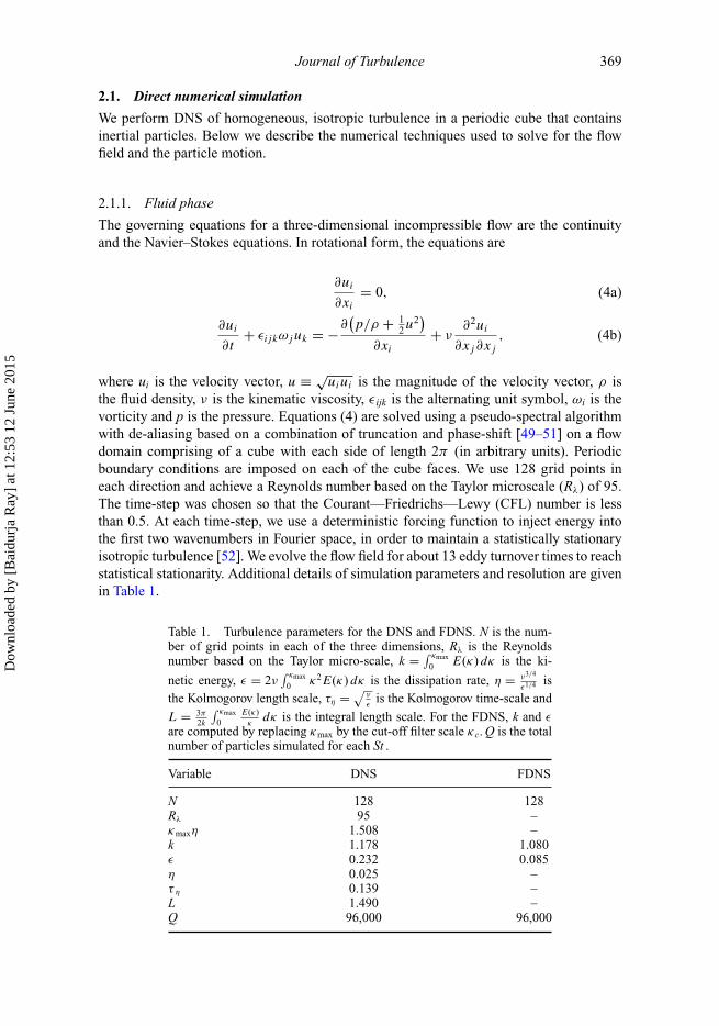
the fluid density, ν is the kinematic viscosity, εijk is the alternating unit symbol, ωi is thevorticity and p is the pressure. Equations (4) are solved using a pseudo-spectral algorithmwith de-aliasing based on a combination of truncation and phase-shift [49–51] on a flowdomain comprising of a cube with each side of length 2π (in arbitrary units). Periodicboundary conditions are imposed on each of the cube faces. We use 128 grid points ineach direction and achieve a Reynolds number based on the Taylor microscale (Rλ) of 95.The time-step was chosen so that the Courant—Friedrichs—Lewy (CFL) number is lessthan 0.5. At each time-step, we use a deterministic forcing function to inject energy intothe first two wavenumbers in Fourier space, in order to maintain a statistically stationaryisotropic turbulence [52]. We evolve the flow field for about 13 eddy turnover times to reachstatistical stationarity. Additional details of simulation parameters and resolution are givenin Table 1.

Table 1. Turbulence parameters for the DNS and FDNS. N is the num-ber of grid points in each of the three dimensions, Rλ is the Reynoldsnumber based on the Taylor micro-scale, k = ∫ κmax

0 E(κ) dκ is the ki-

netic energy, ε = 2ν∫ κmax

0 κ2E(κ) dκ is the dissipation rate, η = ν3/4

ε1/4 isthe Kolmogorov length scale, τη = √

νε

is the Kolmogorov time-scale and

L = 3π2k

∫ κmax

0E(κ)

κdκ is the integral length scale. For the FDNS, k and ε

are computed by replacing κmax by the cut-off filter scale κc. Q is the totalnumber of particles simulated for each St .

Variable DNS FDNS

N 128 128Rλ 95 –κmaxη 1.508 –k 1.178 1.080ε 0.232 0.085η 0.025 –τ η 0.139 –L 1.490 –Q 96,000 96,000

Dow

nloa

ded

by [

Bai

durj

a R

ay]

at 1

2:53

12

June

201

5

370 B. Ray and L.R. Collins

2.1.2. Inertial particle motion

We assume a dilute suspension of inertial particles, which allows us to neglect the feedbackof particle motion on the carrier fluid [53]. We also consider particles whose radius a ismuch smaller than the Kolmogorov length scale η and simulate them as point particles.Furthermore, we assume that the particles are much denser than the surrounding fluid (ρp/ρ f

1), the particle Reynolds numbers are small, and collisions and gravitational settlingare neglected. Under these assumptions, the equations of motion for the particles reduce to[54]

dx(t)

dt= v(t), (5)

dv(t)

dt= u [x(t)] − v(t)

τp

, (6)

where x is the inertial particle position, v is the particle velocity, τp = (2/9) ρpa2

ρf νis the

particle response time and u [x(t)] denotes the fluid velocity at the inertial particle location.We have used 96,000 particles for each of the Stokes numbers considered. These particlesare introduced into the stationary flow field at random positions and with the fluid velocityat those locations. Particles are advanced in time according to (5) and (6) using an improvednumerical scheme recently developed in our group [55,56]. This new algorithm, based onexponential integrators, is second-order accurate in time and can simulate particles witharbitrarily small St accurately. It allows us to use the fluid time-step (dictated by the CFLcondition) to advance the inertial particles, irrespective of St, thereby significantly reducingthe run times for low-St, particles. Fluid velocities at particle locations are obtained usingeighth-order Lagrangian interpolation. We use the DNS velocity field to specify the fluidvelocity seen by the particles in Equations (5) and (6). This gives us an accurate descriptionof the inertial particle positions and velocities. We allow sufficient time (four eddy turnovertimes) for the particles to equilibrate with the flow before collecting statistics. Particlestatistics are averaged over several eddy turnover times.

2.2. Filtering

We perform a low-pass filtering of the DNS velocity field in Fourier space so that all theFourier modes of velocity beyond a preset cut-off wavenumber κc are removed from theflow and only the remaining ‘large scales’ are retained. Such a filtered DNS (FDNS) canbe viewed as a ‘perfect’ LES velocity field, where the large scales are represented exactly,and not subject to any subgrid modelling errors. We apply a sharp spectral filter to theDNS velocity field at each time-step that removes all wavenumbers above κc, yielding thefollowing definition of the filtered velocity:

˜u(κ, t) ={

u(κ, t) |κ | ≤ κc

0 otherwise. (7)

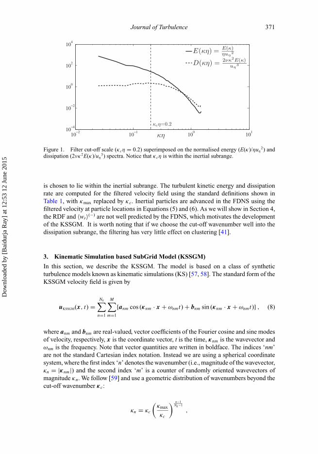
Here, ˜u(κ, t) and u(κ, t) are the Fourier modes of the filtered and unfiltered velocities,respectively, and κcη = 0.2 is the cut-off wavenumber. Figure 1 shows the energy and dissi-pation spectra obtained from the DNS. Notice that the cut-off wavenumber (or filter scale)

Dow

nloa

ded

by [

Bai

durj

a R

ay]

at 1

2:53

12

June

201

5

Journal of Turbulence 371

Figure 1. Filter cut-off scale (κcη = 0.2) superimposed on the normalised energy (E(κ)/ηuη2) and

dissipation (2νκ2E(κ)/uη3) spectra. Notice that κcη is within the inertial subrange.

is chosen to lie within the inertial subrange. The turbulent kinetic energy and dissipationrate are computed for the filtered velocity field using the standard definitions shown inTable 1, with κmax replaced by κc. Inertial particles are advanced in the FDNS using thefiltered velocity at particle locations in Equations (5) and (6). As we will show in Section 4,the RDF and 〈wr〉(−) are not well predicted by the FDNS, which motivates the developmentof the KSSGM. It is worth noting that if we choose the cut-off wavenumber well into thedissipation subrange, the filtering has very little effect on clustering [41].

3. Kinematic Simulation based SubGrid Model (KSSGM)

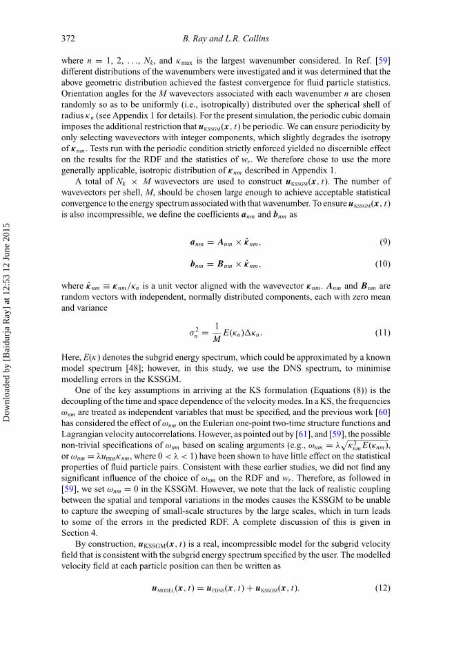
In this section, we describe the KSSGM. The model is based on a class of syntheticturbulence models known as kinematic simulations (KS) [57, 58]. The standard form of theKSSGM velocity field is given by

uKSSGM(x, t) =Nk∑n=1

M∑m=1

{anm cos (κnm · x + ωnmt) + bnm sin (κnm · x + ωnmt)} , (8)

where anm and bnm are real-valued, vector coefficients of the Fourier cosine and sine modesof velocity, respectively, x is the coordinate vector, t is the time, κnm is the wavevector andωnm is the frequency. Note that vector quantities are written in boldface. The indices ‘nm’are not the standard Cartesian index notation. Instead we are using a spherical coordinatesystem, where the first index ‘n’ denotes the wavenumber (i.e., magnitude of the wavevector,κn = |κnm|) and the second index ‘m’ is a counter of randomly oriented wavevectors ofmagnitude κn. We follow [59] and use a geometric distribution of wavenumbers beyond thecut-off wavenumber κc:

κn = κc

(κmax

κc

) n−1Nk−1

,

Dow

nloa

ded

by [

Bai

durj

a R

ay]

at 1

2:53

12

June

201

5

372 B. Ray and L.R. Collins

where n = 1, 2, . . ., Nk, and κmax is the largest wavenumber considered. In Ref. [59]different distributions of the wavenumbers were investigated and it was determined that theabove geometric distribution achieved the fastest convergence for fluid particle statistics.Orientation angles for the M wavevectors associated with each wavenumber n are chosenrandomly so as to be uniformly (i.e., isotropically) distributed over the spherical shell ofradius κn (see Appendix 1 for details). For the present simulation, the periodic cubic domainimposes the additional restriction that uKSSGM(x, t) be periodic. We can ensure periodicity byonly selecting wavevectors with integer components, which slightly degrades the isotropyof κnm. Tests run with the periodic condition strictly enforced yielded no discernible effecton the results for the RDF and the statistics of wr. We therefore chose to use the moregenerally applicable, isotropic distribution of κnm described in Appendix 1.

A total of Nk × M wavevectors are used to construct uKSSGM(x, t). The number ofwavevectors per shell, M, should be chosen large enough to achieve acceptable statisticalconvergence to the energy spectrum associated with that wavenumber. To ensure uKSSGM(x, t)is also incompressible, we define the coefficients anm and bnm as

anm = Anm × κnm, (9)

bnm = Bnm × κnm, (10)

where κnm ≡ κnm/κn is a unit vector aligned with the wavevector κnm. Anm and Bnm arerandom vectors with independent, normally distributed components, each with zero meanand variance

σ 2n = 1

ME(κn)�κn. (11)

Here, E(κ) denotes the subgrid energy spectrum, which could be approximated by a knownmodel spectrum [48]; however, in this study, we use the DNS spectrum, to minimisemodelling errors in the KSSGM.

One of the key assumptions in arriving at the KS formulation (Equations (8)) is thedecoupling of the time and space dependence of the velocity modes. In a KS, the frequenciesωnm are treated as independent variables that must be specified, and the previous work [60]has considered the effect of ωnm on the Eulerian one-point two-time structure functions andLagrangian velocity autocorrelations. However, as pointed out by [61], and [59], the possiblenon-trivial specifications of ωnm based on scaling arguments (e.g., ωnm = λ

√κ3

nmE(κnm),or ωnm = λurmsκnm, where 0 < λ < 1) have been shown to have little effect on the statisticalproperties of fluid particle pairs. Consistent with these earlier studies, we did not find anysignificant influence of the choice of ωnm on the RDF and wr. Therefore, as followed in[59], we set ωnm = 0 in the KSSGM. However, we note that the lack of realistic couplingbetween the spatial and temporal variations in the modes causes the KSSGM to be unableto capture the sweeping of small-scale structures by the large scales, which in turn leadsto some of the errors in the predicted RDF. A complete discussion of this is given inSection 4.

By construction, uKSSGM(x, t) is a real, incompressible model for the subgrid velocityfield that is consistent with the subgrid energy spectrum specified by the user. The modelledvelocity field at each particle position can then be written as

uMODEL(x, t) = uFDNS(x, t) + uKSSGM(x, t). (12)

Dow

nloa

ded

by [

Bai

durj

a R

ay]

at 1

2:53

12

June

201

5

Journal of Turbulence 373

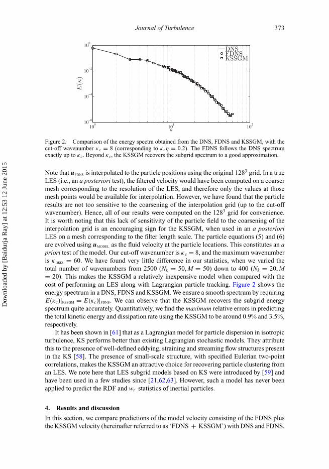
Figure 2. Comparison of the energy spectra obtained from the DNS, FDNS and KSSGM, with thecut-off wavenumber κc = 8 (corresponding to κcη = 0.2). The FDNS follows the DNS spectrumexactly up to κc. Beyond κc, the KSSGM recovers the subgrid spectrum to a good approximation.

Note that uFDNS is interpolated to the particle positions using the original 1283 grid. In a trueLES (i.e., an a posteriori test), the filtered velocity would have been computed on a coarsermesh corresponding to the resolution of the LES, and therefore only the values at thosemesh points would be available for interpolation. However, we have found that the particleresults are not too sensitive to the coarsening of the interpolation grid (up to the cut-offwavenumber). Hence, all of our results were computed on the 1283 grid for convenience.It is worth noting that this lack of sensitivity of the particle field to the coarsening of theinterpolation grid is an encouraging sign for the KSSGM, when used in an a posterioriLES on a mesh corresponding to the filter length scale. The particle equations (5) and (6)are evolved using uMODEL as the fluid velocity at the particle locations. This constitutes an apriori test of the model. Our cut-off wavenumber is κc = 8, and the maximum wavenumberis κmax = 60. We have found very little difference in our statistics, when we varied thetotal number of wavenumbers from 2500 (Nk = 50, M = 50) down to 400 (Nk = 20, M= 20). This makes the KSSGM a relatively inexpensive model when compared with thecost of performing an LES along with Lagrangian particle tracking. Figure 2 shows theenergy spectrum in a DNS, FDNS and KSSGM. We ensure a smooth spectrum by requiringE(κc)|KSSGM = E(κc)|FDNS. We can observe that the KSSGM recovers the subgrid energyspectrum quite accurately. Quantitatively, we find the maximum relative errors in predictingthe total kinetic energy and dissipation rate using the KSSGM to be around 0.9% and 3.5%,respectively.

It has been shown in [61] that as a Lagrangian model for particle dispersion in isotropicturbulence, KS performs better than existing Lagrangian stochastic models. They attributethis to the presence of well-defined eddying, straining and streaming flow structures presentin the KS [58]. The presence of small-scale structure, with specified Eulerian two-pointcorrelations, makes the KSSGM an attractive choice for recovering particle clustering froman LES. We note here that LES subgrid models based on KS were introduced by [59] andhave been used in a few studies since [21,62,63]. However, such a model has never beenapplied to predict the RDF and wr statistics of inertial particles.

4. Results and discussion

In this section, we compare predictions of the model velocity consisting of the FDNS plusthe KSSGM velocity (hereinafter referred to as ‘FDNS + KSSGM’) with DNS and FDNS.

Dow

nloa

ded

by [

Bai

durj

a R

ay]

at 1

2:53

12

June

201

5

374 B. Ray and L.R. Collins

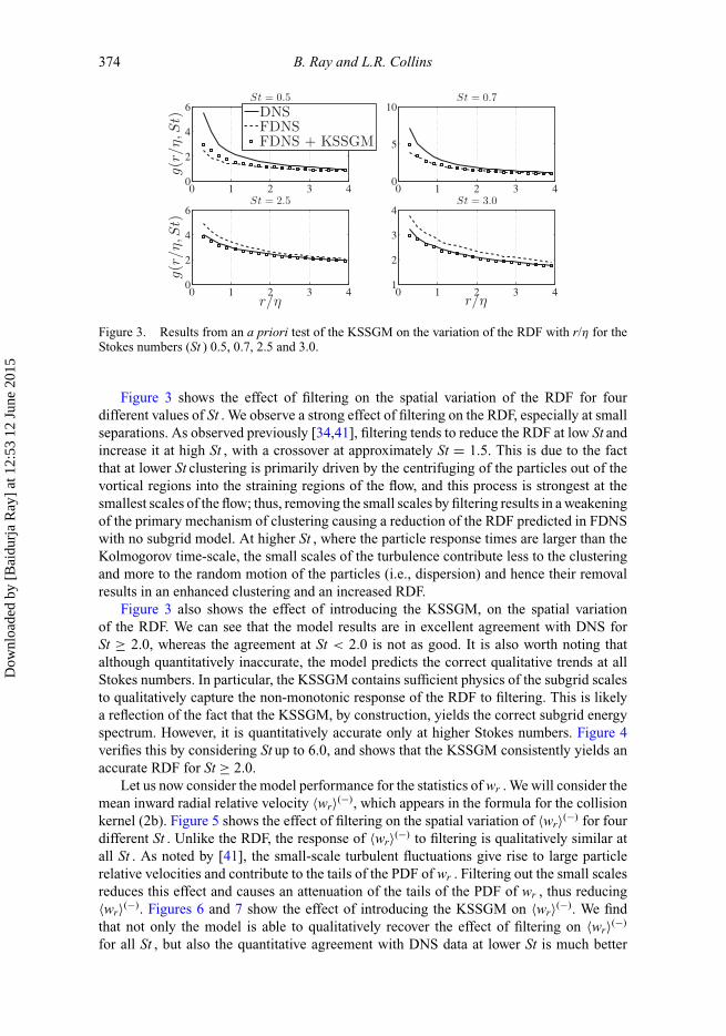
Figure 3. Results from an a priori test of the KSSGM on the variation of the RDF with r/η for theStokes numbers (St ) 0.5, 0.7, 2.5 and 3.0.

Figure 3 shows the effect of filtering on the spatial variation of the RDF for fourdifferent values of St . We observe a strong effect of filtering on the RDF, especially at smallseparations. As observed previously [34,41], filtering tends to reduce the RDF at low St andincrease it at high St , with a crossover at approximately St = 1.5. This is due to the factthat at lower St clustering is primarily driven by the centrifuging of the particles out of thevortical regions into the straining regions of the flow, and this process is strongest at thesmallest scales of the flow; thus, removing the small scales by filtering results in a weakeningof the primary mechanism of clustering causing a reduction of the RDF predicted in FDNSwith no subgrid model. At higher St , where the particle response times are larger than theKolmogorov time-scale, the small scales of the turbulence contribute less to the clusteringand more to the random motion of the particles (i.e., dispersion) and hence their removalresults in an enhanced clustering and an increased RDF.

Figure 3 also shows the effect of introducing the KSSGM, on the spatial variationof the RDF. We can see that the model results are in excellent agreement with DNS forSt ≥ 2.0, whereas the agreement at St < 2.0 is not as good. It is also worth noting thatalthough quantitatively inaccurate, the model predicts the correct qualitative trends at allStokes numbers. In particular, the KSSGM contains sufficient physics of the subgrid scalesto qualitatively capture the non-monotonic response of the RDF to filtering. This is likelya reflection of the fact that the KSSGM, by construction, yields the correct subgrid energyspectrum. However, it is quantitatively accurate only at higher Stokes numbers. Figure 4verifies this by considering St up to 6.0, and shows that the KSSGM consistently yields anaccurate RDF for St ≥ 2.0.

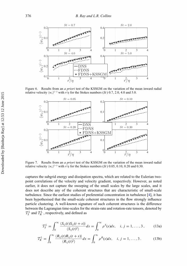
Let us now consider the model performance for the statistics of wr . We will consider themean inward radial relative velocity 〈wr〉(−), which appears in the formula for the collisionkernel (2b). Figure 5 shows the effect of filtering on the spatial variation of 〈wr〉(−) for fourdifferent St . Unlike the RDF, the response of 〈wr〉(−) to filtering is qualitatively similar atall St . As noted by [41], the small-scale turbulent fluctuations give rise to large particlerelative velocities and contribute to the tails of the PDF of wr . Filtering out the small scalesreduces this effect and causes an attenuation of the tails of the PDF of wr , thus reducing〈wr〉(−). Figures 6 and 7 show the effect of introducing the KSSGM on 〈wr〉(−). We findthat not only the model is able to qualitatively recover the effect of filtering on 〈wr〉(−)

for all St , but also the quantitative agreement with DNS data at lower St is much better

Dow

nloa

ded

by [

Bai

durj

a R

ay]

at 1

2:53

12

June

201

5

Journal of Turbulence 375

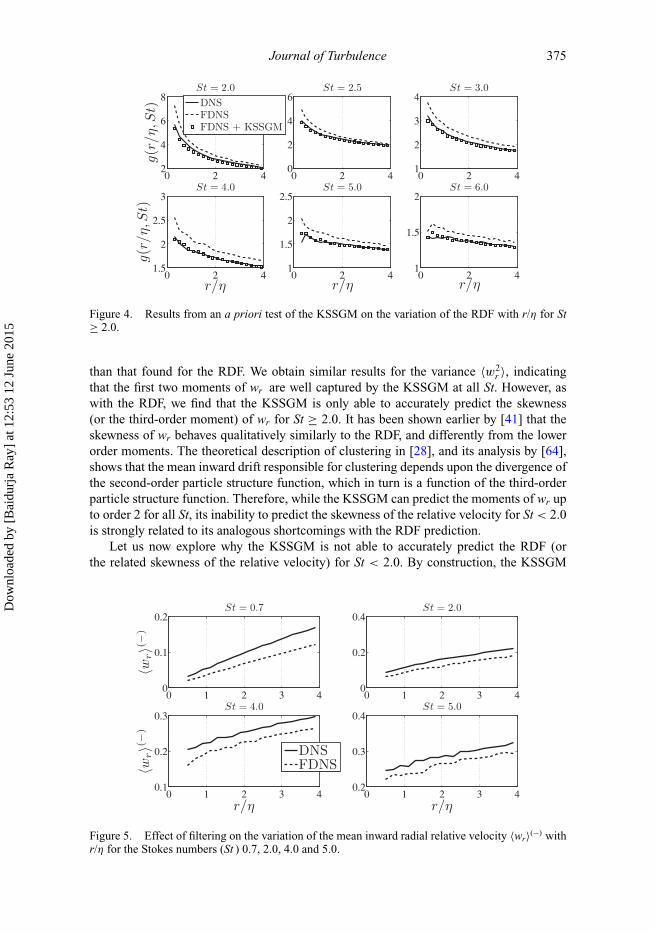
Figure 4. Results from an a priori test of the KSSGM on the variation of the RDF with r/η for St≥ 2.0.

than that found for the RDF. We obtain similar results for the variance 〈w2r 〉, indicating

that the first two moments of wr are well captured by the KSSGM at all St. However, aswith the RDF, we find that the KSSGM is only able to accurately predict the skewness(or the third-order moment) of wr for St ≥ 2.0. It has been shown earlier by [41] that theskewness of wr behaves qualitatively similarly to the RDF, and differently from the lowerorder moments. The theoretical description of clustering in [28], and its analysis by [64],shows that the mean inward drift responsible for clustering depends upon the divergence ofthe second-order particle structure function, which in turn is a function of the third-orderparticle structure function. Therefore, while the KSSGM can predict the moments of wr upto order 2 for all St, its inability to predict the skewness of the relative velocity for St < 2.0is strongly related to its analogous shortcomings with the RDF prediction.

Let us now explore why the KSSGM is not able to accurately predict the RDF (orthe related skewness of the relative velocity) for St < 2.0. By construction, the KSSGM

Figure 5. Effect of filtering on the variation of the mean inward radial relative velocity 〈wr〉(−) withr/η for the Stokes numbers (St ) 0.7, 2.0, 4.0 and 5.0.

Dow

nloa

ded

by [

Bai

durj

a R

ay]

at 1

2:53

12

June

201

5

376 B. Ray and L.R. Collins

Figure 6. Results from an a priori test of the KSSGM on the variation of the mean inward radialrelative velocity 〈wr〉(−) with r/η for the Stokes numbers (St ) 0.7, 2.0, 4.0 and 5.0.

Figure 7. Results from an a priori test of the KSSGM on the variation of the mean inward radialrelative velocity 〈wr〉(−) with r/η for the Stokes numbers (St ) 0.05, 0.10, 0.20 and 0.30.

captures the subgrid energy and dissipation spectra, which are related to the Eulerian two-point correlations of the velocity and velocity gradient, respectively. However, as notedearlier, it does not capture the sweeping of the small scales by the large scales, and itdoes not describe any of the coherent structures that are characteristic of small-scaleturbulence. Since the earliest studies of preferential concentration in turbulence [4], it hasbeen hypothesised that the small-scale coherent structures in the flow strongly influenceparticle clustering. A well-known signature of such coherent structures is the differencebetween the Lagrangian time-scales for the strain-rate and rotation-rate tensors, denoted byT L

S and T LR , respectively, and defined as

T LS =

∫ ∞

0

〈Sij (t)Sij (t + s)〉〈Sij (t)2〉 ds =

∫ ∞

0ρS(s)ds, i, j = 1, . . . , 3 , (13a)

T LR =

∫ ∞

0

〈Rij (t)Rij (t + s)〉〈Rij (t)2〉 ds =

∫ ∞

0ρR(s)ds, i, j = 1, . . . , 3 . (13b)

Dow

nloa

ded

by [

Bai

durj

a R

ay]

at 1

2:53

12

June

201

5

Journal of Turbulence 377

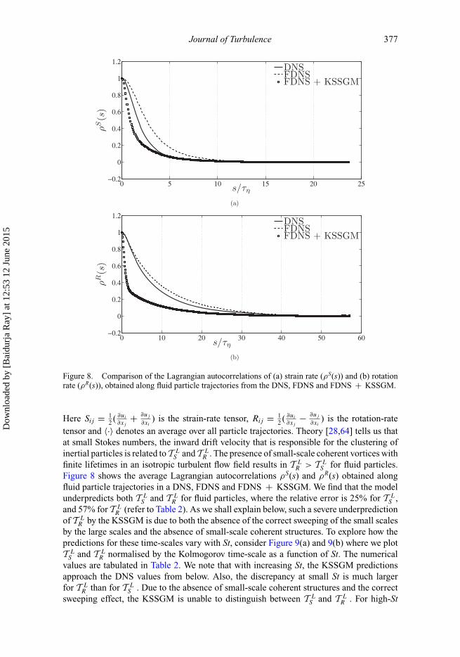
Figure 8. Comparison of the Lagrangian autocorrelations of (a) strain rate (ρS(s)) and (b) rotationrate (ρR(s)), obtained along fluid particle trajectories from the DNS, FDNS and FDNS + KSSGM.

Here Sij = 12 ( ∂ui

∂xj+ ∂uj

∂xi) is the strain-rate tensor, Rij = 1

2 ( ∂ui

∂xj− ∂uj

∂xi) is the rotation-rate

tensor and 〈·〉 denotes an average over all particle trajectories. Theory [28,64] tells us thatat small Stokes numbers, the inward drift velocity that is responsible for the clustering ofinertial particles is related to T L

S and T LR . The presence of small-scale coherent vortices with

finite lifetimes in an isotropic turbulent flow field results in T LR > T L

S for fluid particles.Figure 8 shows the average Lagrangian autocorrelations ρS(s) and ρR(s) obtained alongfluid particle trajectories in a DNS, FDNS and FDNS + KSSGM. We find that the modelunderpredicts both T L

S and T LR for fluid particles, where the relative error is 25% for T L

S ,and 57% for T L

R (refer to Table 2). As we shall explain below, such a severe underpredictionof T L

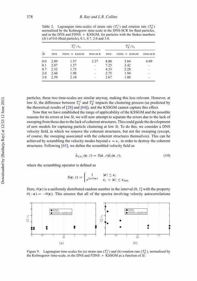
R by the KSSGM is due to both the absence of the correct sweeping of the small scalesby the large scales and the absence of small-scale coherent structures. To explore how thepredictions for these time-scales vary with St, consider Figure 9(a) and 9(b) where we plotT L

S and T LR normalised by the Kolmogorov time-scale as a function of St. The numerical

values are tabulated in Table 2. We note that with increasing St, the KSSGM predictionsapproach the DNS values from below. Also, the discrepancy at small St is much largerfor T L

R than for T LS . Due to the absence of small-scale coherent structures and the correct

sweeping effect, the KSSGM is unable to distinguish between T LS and T L

R . For high-St

Dow

nloa

ded

by [

Bai

durj

a R

ay]

at 1

2:53

12

June

201

5

378 B. Ray and L.R. Collins

Table 2. Lagrangian time-scales of strain rate (T LS ) and rotation rate (T L

R )normalised by the Kolmogorov time-scale in the DNS-SCR for fluid particles,and in the DNS and FDNS + KSSGM, for particles with the Stokes numbers(St ) of 0.0 (fluid particle), 0.1, 0.7, 2.0 and 3.0.

T LS /τη T L

R /τη

St DNS FDNS + KSSGM DNS-SCR DNS FDNS + KSSGM DNS-SCR

0.0 2.09 1.57 2.27 8.80 3.84 6.090.1 2.07 1.57 – 7.25 3.42 –0.7 2.32 1.73 – 4.33 2.28 –2.0 2.44 1.98 – 2.75 1.94 –3.0 2.59 2.10 – 2.67 1.88 –

particles, these two time-scales are similar anyway, making this less relevant. However, atlow St, the difference between T L

S and T LR impacts the clustering process (as predicted by

the theoretical results of [28] and [64]), and the KSSGM cannot capture this effect.Now that we have established the range of applicability of the KSSGM and the possible

reasons for its errors at low St, we will now attempt to separate the errors due to the lack ofsweeping from those due to the lack of coherent structures. This could guide the developmentof new models for capturing particle clustering at low St. To do this, we consider a DNSvelocity field, in which we remove the coherent structures, but not the sweeping (except,of course, the sweeping associated with the coherent structures themselves). This can beachieved by scrambling the velocity modes beyond κ = κc in order to destroy the coherentstructures. Following [65], we define the scrambled velocity field as

uSCR,i(κ, t) = S(κ, t)ui(κ, t), (14)

where the scrambling operator is defined as

S(κ, t) ={

1 |κ | ≤ κc

e2πiθ(κ) κc < |κ | ≤ κmax

Here, θ (κ) is a uniformly distributed random number in the interval (0, 1] with the propertyθ (−κ) = −θ (κ). This ensures that all of the spectra involving velocity autocorrelations

Figure 9. Lagrangian time-scales for (a) strain rate (T LS ) and (b) rotation rate (T L

R ), normalised bythe Kolmogorov time-scale, in the DNS and FDNS + KSSGM as a function of St.

Dow

nloa

ded

by [

Bai

durj

a R

ay]

at 1

2:53

12

June

201

5

Journal of Turbulence 379

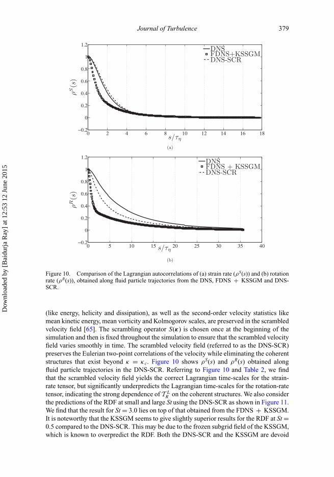
Figure 10. Comparison of the Lagrangian autocorrelations of (a) strain rate (ρS(s)) and (b) rotationrate (ρR(s)), obtained along fluid particle trajectories from the DNS, FDNS + KSSGM and DNS-SCR.

(like energy, helicity and dissipation), as well as the second-order velocity statistics likemean kinetic energy, mean vorticity and Kolmogorov scales, are preserved in the scrambledvelocity field [65]. The scrambling operator S(κ) is chosen once at the beginning of thesimulation and then is fixed throughout the simulation to ensure that the scrambled velocityfield varies smoothly in time. The scrambled velocity field (referred to as the DNS-SCR)preserves the Eulerian two-point correlations of the velocity while eliminating the coherentstructures that exist beyond κ = κc. Figure 10 shows ρS(s) and ρR(s) obtained alongfluid particle trajectories in the DNS-SCR. Referring to Figure 10 and Table 2, we findthat the scrambled velocity field yields the correct Lagrangian time-scales for the strain-rate tensor, but significantly underpredicts the Lagrangian time-scales for the rotation-ratetensor, indicating the strong dependence of T L

R on the coherent structures. We also considerthe predictions of the RDF at small and large St using the DNS-SCR as shown in Figure 11.We find that the result for St = 3.0 lies on top of that obtained from the FDNS + KSSGM.It is noteworthy that the KSSGM seems to give slightly superior results for the RDF at St =0.5 compared to the DNS-SCR. This may be due to the frozen subgrid field of the KSSGM,which is known to overpredict the RDF. Both the DNS-SCR and the KSSGM are devoid

Dow

nloa

ded

by [

Bai

durj

a R

ay]

at 1

2:53

12

June

201

5

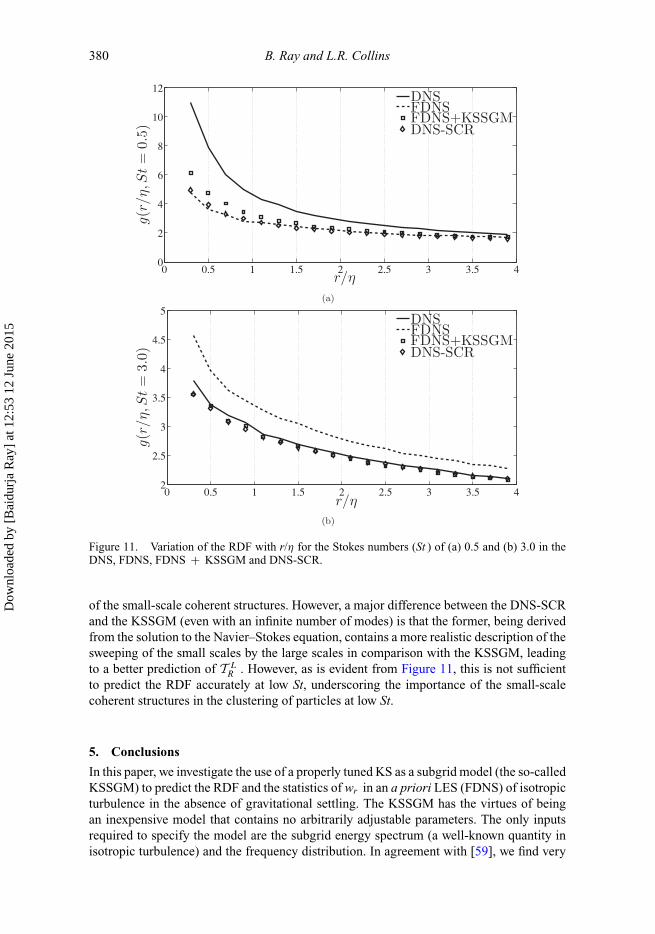
380 B. Ray and L.R. Collins

Figure 11. Variation of the RDF with r/η for the Stokes numbers (St ) of (a) 0.5 and (b) 3.0 in theDNS, FDNS, FDNS + KSSGM and DNS-SCR.

of the small-scale coherent structures. However, a major difference between the DNS-SCRand the KSSGM (even with an infinite number of modes) is that the former, being derivedfrom the solution to the Navier–Stokes equation, contains a more realistic description of thesweeping of the small scales by the large scales in comparison with the KSSGM, leadingto a better prediction of T L

R . However, as is evident from Figure 11, this is not sufficientto predict the RDF accurately at low St, underscoring the importance of the small-scalecoherent structures in the clustering of particles at low St.

5. Conclusions

In this paper, we investigate the use of a properly tuned KS as a subgrid model (the so-calledKSSGM) to predict the RDF and the statistics of wr in an a priori LES (FDNS) of isotropicturbulence in the absence of gravitational settling. The KSSGM has the virtues of beingan inexpensive model that contains no arbitrarily adjustable parameters. The only inputsrequired to specify the model are the subgrid energy spectrum (a well-known quantity inisotropic turbulence) and the frequency distribution. In agreement with [59], we find very

Dow

nloa

ded

by [

Bai

durj

a R

ay]

at 1

2:53

12

June

201

5

Journal of Turbulence 381

little sensitivity to the selection of the frequency distribution, and therefore set them tozero. We show that the KSSGM is able to quantitatively predict the RDF only for St ≥ 2.0.Furthermore, the KSSGM can accurately predict the moments of wr up to order 2 at all St,but can capture the skewness of wr only for St ≥ 2.0. Since the RDF is closely related to theskewness of wr [28,41,64], the limitations with respect to the predictions of both statisticsare related. One possible explanation for this is that the KSSGM is unable to properlycapture the difference between T L

S and T LR , which at low St occurs due to the presence of

small-scale coherent structures and the sweeping of the small scales by the large scales,both of which are not accounted for in the KSSGM. Since there is little difference betweenthese time-scales for St ≥ 2.0 (T L

S ≈ T LR ), the KSSGM works well in that regime. By using

a DNS field that is scrambled beyond κ = κc, we show that describing the small-scalecoherent structures is essential to correct these time-scales and accurately predict the RDFat low St. We hope that such understanding will assist in future developments of subgridmodels aimed at predicting clustering for St < 2.0.

Finally, we note an important advantage of the KSSGM is that it has been adaptedto inhomogeneous flows [21, 66]. It is a natural extension of this work to evaluate thepredictions from the KSSGM in these more complex flows.

AcknowledgementsThe authors gratefully acknowledge Andrew D. Bragg for insightful inputs throughout the course ofthis work. The authors also gratefully acknowledge the Texas Advanced Computing Center (TACC)at The University of Texas at Austin for providing HPC resources on Ranger and Stampede that havecontributed to the research results reported in this paper..

FundingThis study was supported by the National Science Foundation [grant number CBET 0756510],[grant number CBET 0967349]. This work used the Extreme Science and Engineering DiscoveryEnvironment (XSEDE), which is supported by the National Science Foundation [grant number OCI-1053575].

References[1] M.R. Maxey, The gravitational settling of aerosol particles in homogeneous turbulence and

random flow fields, J. Fluid Mech. 174 (1987), pp. 441–465.[2] K.D. Squires and J.K. Eaton, Preferential concentration of particles by turbulence, Phys. Fluids

A 3 (1991), pp. 1169–1178.[3] L.P. Wang and M.R. Maxey, Settling velocity and concentration distribution of heavy particles

in homogeneous isotropic turbulence, J. Fluid Mech. 256 (1993), pp. 27–68.[4] J.K. Eaton and J.R. Fessler, Preferential concentration of particles by turbulence, Int. J. Multi-

phase Flow 20 (1994), pp. 169–209.[5] S. Sundaram and L.R. Collins, Collision statistics in an isotropic, particle-laden turbulent

suspension. Part I. Direct numerical simulations, J. Fluid Mech. 335 (1997), pp. 75–109.[6] J.R. Fessler, J.D. Kulick, and J.K. Eaton, Preferential concentration of heavy particles in a

turbulent channel flow, Phys. Fluids 6 (1994), pp. 3742–3749.[7] J.P.L.C. Salazar, J. de Jong, L. Cao, S. Woodward, H. Meng, and L.R. Collins, Experimental and

numerical investigation of inertial particle clustering in isotropic turbulence, J. Fluid Mech.600 (2008), pp. 245–256.

[8] E.W. Saw, R.A. Shaw, S. Ayyalasomayajula, P.Y. Chuang, and A. Gylfason, Inertial clusteringof particles in high-Reynolds-number turbulence, Phys. Rev. Lett. 100 (2008), p. 214501.

[9] M. Gibert, H. Xu, and E. Bodenschatz, Where do small, weakly inertial particles go in aturbulent flow? J. Fluid Mech. 698 (2012), pp. 160–167.

Dow

nloa

ded

by [

Bai

durj

a R

ay]

at 1

2:53

12

June

201

5

382 B. Ray and L.R. Collins

[10] C.P. Bateson and A. Aliseda, Wind tunnel measurements of the preferential concentrationof inertial droplets in homogeneous isotropic turbulence, Exp. Fluids 52 (2012), pp. 1373–1387.

[11] E.W. Saw, R.A. Shaw, J.P.L.C. Salazar, and L.R. Collins, Spatial clustering of polydisperseinertial particles in turbulence: II. Comparing simulation with experiment, New J. Phys. 14(2012), p. 105031.

[12] R.A. Shaw, W.C. Reade, L.R. Collins, and J. Verlinde, Preferential concentration of clouddroplets by turbulence: Effects on the early evolution of cumulus cloud droplet spectra,J. Atmos. Sci. 55 (1998), pp. 1965–1976.

[13] W.C. Reade and L.R. Collins, A numerical study of the particle size distribution of an aerosolundergoing turbulent coagulation, J. Fluid Mech. 415 (2000), pp. 45–64.

[14] G. Falkovich, A. Fouxon, and M.G. Stepanov, Acceleration of rain initiation by cloud turbu-lence, Nature 419 (2002), pp. 151–154.

[15] R.A. Shaw, Particle-turbulence interactions in atmospheric clouds, Annu. Rev. Fluid Mech.35 (2003), pp. 183–227.

[16] B.J. Devenish, P. Bartello, J.L. Brenguier, L.R. Collins, W.W. Grabowski, R.H.A. IJzermans,S.P. Malinowski, M.W. Reeks, J.C. Vassilicos, L.P. Wang, and Z. Warhaft, Droplet growth inwarm turbulent clouds, Quart. J. Royal Meteor. Soc. 138 (2012), pp. 1401–1429.

[17] W.W. Grabowski and L.P. Wang, Growth of cloud droplets in a turbulent environment, Ann.Rev. Fluid Mech. 45 (2013), pp. 293–324.

[18] O. Ayala, B. Rosa, L.P. Wang, and W.W. Grabowski, Effects of turbulence on the geometriccollision rate of sedimenting droplets. Part 1. Results from direct numerical simulation, NewJ. Phys. 10 (2008), p. 075015.

[19] L. Pan and P. Padoan, Relative velocity of inertial particles in turbulent flows, J. Fluid Mech.661 (2010), pp. 73–107.

[20] L. Pan, P. Padoan, J. Scalo, A.G. Kritsuk, and M.L. Norman, Turbulent clustering of protoplan-etary dust and planetesimal formation, Astrophys. J. 740 (2011), p. 6.

[21] M.A.I. Khan, X.Y. Luo, F.C.G.A. Nicolleau, P.G. Tucker, and G. Lo Iacono, Effects of LESsub-grid flow structure on particle deposition in a plane channel with a ribbed wall, Int. J.Num. Meth. Biomed. Eng. 26 (2010), pp. 999–1015.

[22] D.A. McQuarrie, Statistical Mechanics, Harper & Row, New York, 1976.[23] L.P. Wang, A.S. Wexler, and Y. Zhou, Statistical mechanical description and modeling of

turbulent collision of inertial particles, J. Fluid Mech. 415 (2000), pp. 117–153.[24] O. Ayala, B. Rosa, and L.P. Wang, Effects of turbulence on the geometric collision rate

of sedimenting droplets. Part 2. Theory and parameterization, New J. Phys. 10 (2008),p. 075016.

[25] J. de Jong, J.P.L.C. Salazar, L. Cao, S.H. Woodward, L.R. Collins, and H. Meng, Measurementof inertial particle clustering and relative velocity statistics in isotropic turbulence usingholographic imaging, Int. J. Multiphase Flow 36 (2010), pp. 324–332.

[26] J. Bec, L. Biferale, M. Cencini, A.S. Lanotte, and F. Toschi, Intermittency in the velocitydistribution of heavy particles in turbulence, J. Fluid Mech. 646 (2010), pp. 527–536.

[27] J. Chun, D.L. Koch, S. Rani, A. Ahluwalia, and L.R. Collins, Clustering of aerosol particles inisotropic turbulence, J. Fluid Mech. 536 (2005), pp. 219–251.

[28] L.I. Zaichik and V.M. Alipchenkov, Statistical models for predicting pair dispersion andparticle clustering in isotropic turbulence and their applications, New J. Phys. 11 (2009),p. 103018.

[29] J.P.L.C. Salazar and L.R. Collins, Inertial particle relative velocity statistics in homogeneousisotropic turbulence, J. Fluid Mech. 696 (2012), pp. 45–66.

[30] Q. Wang and K.D. Squires, Large eddy simulation of particle-laden turbulent channel flow,Phys. Fluids 8 (1996), pp. 1207–1223.

[31] Q. Wang and K. Squires, Large eddy simulation of particle deposition in a vertical turbulentchannel flow, Int. J. Multiphase Flow 22 (1996), pp. 667–683.

[32] V. Armenio, U. Piomelli, and V. Fiorotto, Effect of the subgrid scales on particle motion, Phys.Fluids 11 (1999), pp. 3030–3042.

[33] M. Boivin, O. Simonin, and K.D. Squires, On the prediction of gas-solid flows with two-waycoupling using large eddy simulation, Phys. Fluids 12 (2000), pp. 2080–2090.

[34] P. Fede and O. Simonin, Numerical study of the subgrid fluid turbulence effects on the statisticsof heavy colliding particles, Phys. Fluids 18 (2006), p. 045103.

Dow

nloa

ded

by [

Bai

durj

a R

ay]

at 1

2:53

12

June

201

5

Journal of Turbulence 383

[35] C. Marchioli, M.V. Salvetti, and A. Soldati, Some issues concerning large-eddy simulation ofinertial particle dispersion in turbulent bounded flows, Phys. Fluids 20 (2008), p. 040603.

[36] J. Pozorski and S.V. Apte, Filtered particle tracking in isotropic turbulence and stochasticmodeling of subgrid-scale dispersion, Int. J. Multiphase Flow 35 (2009), pp. 118–128.

[37] J. Capecelatro, P. Pepiot, and O. Desjardins, Numerical characterization and modeling ofparticle clustering in wall-bounded vertical risers, Chem. Eng. J. 245 (2014), pp. 295–310.

[38] B. Shotorban and F. Mashayek, Modeling subgrid-scale effects on particles by approximatedeconvolution, Phys. Fluids 17 (2005), p. 081701.

[39] J.G.M. Kuerten, Subgrid modeling in particle-laden channel flow, Phys. Fluids 18 (2006),p. 025108.

[40] G. Jin, G.W. He, and L.P. Wang, Large-eddy simulation of turbulent collision of heavy particlesin isotropic turbulence, Phys. Fluids 22 (2010), p. 055106.

[41] B. Ray and L.R. Collins, Preferential concentration and relative velocity statistics of inertialparticles in Navier-Stokes turbulence with and without filtering, J. Fluid Mech. 680 (2011), pp.488–510.

[42] C. Gobert and M. Manhart, Subgrid modelling for particle-LES by Spectrally Optimised Inter-polation (SOI), J. Comp. Phys. 230 (2011), pp. 7796–7820.

[43] B. Shotorban and F. Mashayek, A stochastic model for particle motion in large-eddy simulation,J. Turb. 7 (2006), p. N11.

[44] B. Shotorban and F. Mashayek, On Stochastic Modeling of Heavy Particle Dispersion inLarge-Eddy Simulation of Two-Phase Turbulent Flow, IUTAM Symposium on ComputationalMultiphase Flow Vol. 81, Part V, Springer, Dordrecht, 2006.

[45] P. Fede, O. Simonin, P. Villedieu, and K.D. Squires, Stochastic Modeling of Turbulent SubgridFluid Velocity Along Inertia Particle Trajectories, Proceedings of the 2006 CTR SummerProgram, Center for Turbulence Research, Stanford, CA, 2006.

[46] M.J. Cernick, Particle subgrid scale modeling in large-eddy simulation of particle-laden tur-bulence, Master’s thesis, McMaster University, 2013.

[47] B. Ray and L.R. Collins, Investigation of sub-Kolmogorov inertial particle pair dynamics inturbulence using novel satellite particle simulations, J. Fluid Mech. 720 (2013), pp. 192–211.

[48] S.B. Pope Turbulent Flows, Cambridge University Press, New York, 2000.[49] G.S. Patterson and S.A. Orszag, Spectral calculation of isotropic turbulence: Efficient removal

of aliasing interactions, Phys. Fluids 14 (1971), pp. 2538–2541.[50] R.W. Johnson (ed.), The Handbook of Fluid Dynamics, CRC Press, New York, 1998.[51] K.A. Brucker, J.C. Isaza, T. Vaithianathan, and L.R. Collins, Efficient algorithm for simulating

homogeneous turbulent shear flow without remeshing, J. Comp. Phys. 225 (2007), pp. 20–32.

[52] A. Witkowska, J.G. Brasseur, and D. Juve, Numerical study of noise from isotropic turbulence,J. Comput. Acoust. 5 (1997), pp. 317–336.

[53] S. Sundaram and L.R. Collins, A numerical study of the modulation of isotropic turbulence bysuspended particles, J. Fluid Mech. 379 (1999), pp. 105–143.

[54] M.R. Maxey and J.J. Riley, Equation of motion for a small rigid sphere in a nonuniform flow,Phys. Fluids 26 (1983), pp. 883–889.

[55] P.J. Ireland, T. Vaithianathan, and L.R. Collins, Massively parallel simulations of inertial parti-cles in high-Reynolds-number turbulence, Proceedings of the Seventh International Conferenceon Computational Fluid Dynamics, Hawaii, 2012.

[56] P.J. Ireland, T. Vaithianathan, P.S. Sukheswalla, B. Ray, and L.R. Collins, Highly paral-lel particle-laden flow solver for turbulence research, Comput. Fluids 76 (2013), pp. 170–177.

[57] R.H. Kraichnan, Diffusion by a random velocity field, Phys. Fluids 13 (1970), pp. 22–31.[58] J.C.H. Fung, J.C.R. Hunt, N.A. Malik, and R.J. Perkins, Kinematic simulation of homoge-

neous turbulence by unsteady random Fourier modes, J. Fluid Mech. 236 (1992), pp. 281–318.

[59] P. Flohr and J.C. Vassilicos, A scalar subgrid model with flow structure for large-eddy simula-tions of scalar variances, J. Fluid Mech. 407 (2000), pp. 315–349.

[60] D.R. Osborne, J.C. Vassilicos, and J.D. Haigh, One-particle two-time diffusion in three-dimensional homogeneous isotropic turbulence, Phys. Fluids 17 (2005), p. 035104.

Dow

nloa

ded

by [

Bai

durj

a R

ay]

at 1

2:53

12

June

201

5

384 B. Ray and L.R. Collins

[61] N.A. Malik and J.C. Vassilicos, A Lagrangian model for turbulent dispersion with turbulent-likeflow structure: Comparison with direct numerical simulation for two-particle statistics, Phys.Fluids 11 (1999), pp. 1572–1580.

[62] G. Lacorata, A. Mazzino, and U. Rizza, 3D chaotic model for subgrid turbulent dispersion inlarge eddy simulations, J. Turbul. 65 (2008), pp. 2389–2401.

[63] H.D. Yao and G.W. He, A kinematic subgrid scale model for large-eddy simulation ofturbulence-generated sound, J. Turbul. 10 (2009), pp. 1–14.

[64] A.D. Bragg and L.R. Collins, New insights from comparing statistical theories for inertialparticles in turbulence. Part I. Spatial distribution of particles, New J. Phys., in press (2014).

[65] M. Ulitsky and L.R. Collins, Relative importance of coherent structures vs background tur-bulence in the propagation of a premixed flame, Combust. Flame 111 (1997), pp. 257–275.

[66] N. Clark and J. Vassilicos, Kinematic simulation of fully developed turbulent channel flow,Flow Turbul. Combust. 86 (2011), pp. 263–293.

[67] E.W. Weisstein, Sphere Point Picking, MathWorld – A Wolfram Web Resource, 2013; softwareavailable at http://mathworld.wolfram.com/SpherePointPicking.html.

Appendix 1. Isotropic specification of κ

In order to generate isotropic statistics with the KSSGM, we require an isotropic specification of thewavevectors κnm [58]. The specification of κnm usually described in the literature (see [63]) is givenby

κnm = |κnm|(sin θnm cos φnm, sin θnm sin φnm, cos θnm), (A1)

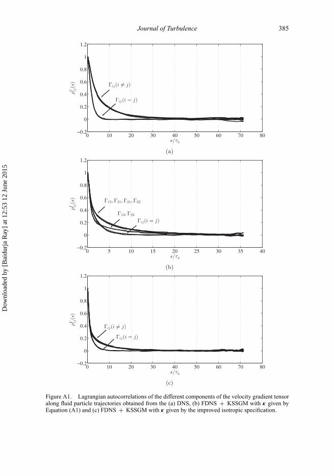
where θnm ∈ [0, 2π ] and φnm ∈ [0, π ] are uniformly distributed random angles. We can show thatthis specification does not generate a truly isotropic distribution of κ . For example, if we considera sphere with a radius κnm, then for m = 1, . . ., M, Equation (A1) generates samples of vectorsκnm that are clustered near the poles of the sphere [67], resulting in anisotropic flow statistics.For example, consider the velocity gradient tensor �, which is a small-scale statistic likely to beinfluenced by the isotropy of the KSSGM flow field. If we consider the Lagrangian autocorrelationsρ�

ij (s) = 〈�ij (t)�ij (t+s)〉〈�ij (t)2〉 ∀ i, j = 1, 2, 3, of each component of �, isotropy implies that we will get

two distinct sets of curves, one for the diagonal terms ρ�ii (s), ∀ i = 1, 2, 3, and the other for the

off-diagonal terms ρ�ij (s), ∀ i, j = 1, 2, 3 (i �= j ). Figure A1(a) shows this from DNS data, whereas

Figure A1(b) shows the same curves using FDNS + KSSGM with κ specified by Equation (A1).We find that the off-diagonal components of � generated by this method are not truly isotropic. Asimple algorithm to generate an isotropic κnm uses Equation (A1) but with a different choice of theangles:

(1) Choose uniformly distributed random numbers cos θnm ∈ [ − 1, 1], φnm ∈ [0, 2π ], and definesin θnm =

√1 − cos2 θnm.

(2) Generate an isotropic distribution on a sphere of radius |κnm|:

κnm = |κnm|(sin θnm cos φnm, sin θnm sin φnm, cos θnm). (A2)

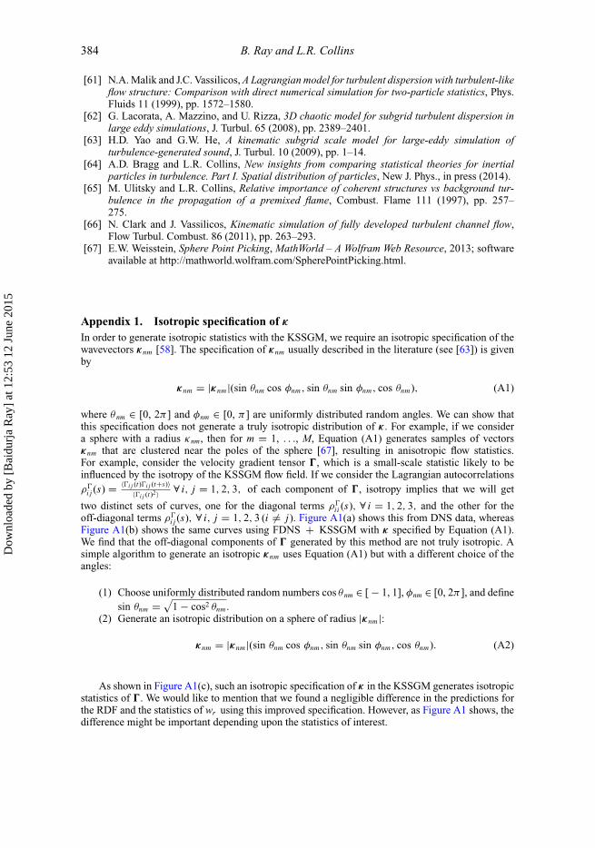
As shown in Figure A1(c), such an isotropic specification of κ in the KSSGM generates isotropicstatistics of �. We would like to mention that we found a negligible difference in the predictions forthe RDF and the statistics of wr using this improved specification. However, as Figure A1 shows, thedifference might be important depending upon the statistics of interest.

Dow

nloa

ded

by [

Bai

durj

a R

ay]

at 1

2:53

12

June

201

5

Journal of Turbulence 385

Figure A1. Lagrangian autocorrelations of the different components of the velocity gradient tensoralong fluid particle trajectories obtained from the (a) DNS, (b) FDNS + KSSGM with κ given byEquation (A1) and (c) FDNS + KSSGM with κ given by the improved isotropic specification.

Dow

nloa

ded

by [

Bai

durj

a R

ay]

at 1

2:53

12

June

201

5