Assessment of Inertia in Indian Power System - POSOCO

Power System Operation Corporation Limited

in collaboration with

Indian Institute of Technology Bombay

JANUARY 2022

Report on

Assessment of Inertia in

Indian Power System

Disclaimer

Precautions have been taken by Power System Operation Corporation (POSOCO) and Indian Institute

of Technology Bombay (IITB) to ensure the accuracy of data / information and the data / information

in this report is believed to be accurate, reliable and complete. However, before relying on the

information material from this report, users are advised to ensure its accuracy, currency,

completeness and relevance for their purposes, and, in this respect, POSOCO and IITB shall not be

responsible for any errors or omissions. All information is provided without warranty of any kind.

POSOCO and IITB disclaim all express, implied, and statutory warranties of any kind to user and/or any

third party, including warranties as to accuracy, timeliness, completeness, merchantability, or fitness

for any purpose. POSOCO and IITB have no liability in tort, contract, or otherwise to user and/or third

party. Further, POSOCO and/or IITB shall, under no circumstances, be liable to user, and/or any third

party, for any lost profits or lost opportunity, indirect, special, consequential, incidental, or punitive

damages whatsoever, even if POSOCO and/or IITB have been advised of the possibility of such

damages.

1

Table of Contents

List of Figures ................................................................................................................................................. 3

List of Tables ................................................................................................................................................... 5

List of Contributors ....................................................................................................................................... 11

Executive Summary ...................................................................................................................................... 13

Indian Power System in Numbers .................................................................................................................. 17

Abbreviations and Symbols ........................................................................................................................... 18

Chapter 1: Introduction ............................................................................................................................ 19

Chapter 2: Inertia: Theoretical Background ............................................................................................... 23

2.1 Concept of Inertia ....................................................................................................................................................................................... 23

2.2 Inertia of power system ............................................................................................................................................................................. 24

2.3 Inertial response in power system observed through grid frequency ........................................................................................... 28

2.4 Challenges in power system operation under low inertia................................................................................................................ 31

2.5 Classification of inertia estimation methods ........................................................................................................................................ 33

Chapter 3: Power System Inertia Estimation – International Practices ........................................................ 37

3.1 North American Electric Reliability Corporation ............................................................................................................................... 37

3.2 Australian Energy Market Operator (AEMO) ..................................................................................................................................... 38

3.3 ENTSO-E – future system inertia ........................................................................................................................................................... 40

3.4 Ireland ............................................................................................................................................................................................................ 43

3.5 National Grid UK System ......................................................................................................................................................................... 44

3.6 Inferences for estimation of inertia of Indian power system ........................................................................................................... 45

Chapter 4: Inertia of Generating Units in India .......................................................................................... 46

4.1 Sources of Inertia in Power system ........................................................................................................................................................ 46

4.2 Inertia contribution from Renewable Energy sources ....................................................................................................................... 55

4.3 Synthetic Inertia from non-synchronous generation sources .......................................................................................................... 59

Chapter 5: Measurement based System Inertia Estimation ........................................................................ 62

5.1 Literature Survey on evaluation of inertia estimation methods from measurement data ....................................................... 62

5.2 Approach for measurement-based inertia estimation in Indian power system .......................................................................... 66

5.3 Challenges in measurement based inertia estimation ........................................................................................................................ 70

Chapter 6: Inertia Estimation in Indian Power System ............................................................................... 73

6.1 Inertia Estimation Results from Frequency Measurements .............................................................................................................. 73

6.3 Impact on Power System Inertia during Covid-19 Pandemic .......................................................................................................... 77

6.4 Minimum inertia requirement for the Indian power system ............................................................................................................ 78

6.5 Summary ........................................................................................................................................................................................................ 79

2

Chapter 7: Online Inertia Monitoring in Indian Grid ................................................................................... 80

7.1 Estimation based on sum of known inertia constants ....................................................................................................................... 80

7.2 Estimation based on continuous or ambient measurement ............................................................................................................. 80

7.3 Online Inertia Estimation at RLDCs and NLDC ................................................................................................................................. 80

Chapter 8: Frequency Response Characteristics in Indian Power System .................................................... 87

8.1 Primary Frequency Response Requirement ......................................................................................................................................... 87

8.2 Estimation of Frequency Response Indicators ..................................................................................................................................... 87

Chapter 9: RE Driven Inertia Trends and Simulation Analysis of Indian Power System ................................ 93

9.1 Effect of RE capacity on inertia ................................................................................................................................................................ 93

9.2 Simulation studies using all India model................................................................................................................................................. 98

9.3 Summary ..................................................................................................................................................................................................... 103

Chapter 10: Recommendations and Way Forward ................................................................................. 105

10.1 Technical Recommendations: ............................................................................................................................................................. 105

10.2 Regulatory and Policy Recommendations: ...................................................................................................................................... 106

Bibliography ............................................................................................................................................... 108

Annexure-1: Inertia Constant of Generators Region wise ............................................................................. 110

Annexure-2: Synchronous Condensers ......................................................................................................... 113

3

List of Figures

Figure 1.1 Stages of power system frequency response after a disturbance ........................................................ 19 Figure 1.2 Frequency response during 12 March 2014 event ............................................................................... 20 Figure 1.3 Frequency response during 23 April 2018 event .................................................................................. 21 Figure 1.4 Frequency response during 28 May 2020 event .................................................................................. 21 Figure 2.1 Power system inertia and water tank analogy .................................................................................... 25 Figure 2.2 Impedance diagram of the single machine infinite bus system ........................................................... 26 Figure 2.3 Drive train of a thermal power plant with three pressure stages. ....................................................... 28 Figure 2.4 Impact of diminishing inertia on system frequency response [2] ......................................................... 29 Figure 2.5 Frequency response indicators ............................................................................................................. 30 Figure 2.6 Classification of inertia estimation methods ........................................................................................ 34 Figure 2.7 Sub classification of online inertia estimation methods....................................................................... 35 Figure 3.1 (a) Fast FCAS requirement & (b) FCAS availability with inertia (AEMO) .............................................. 39 Figure 3.2 Maximum frequency deviation relative to power imbalance and estimated kinetic energy ............... 42 Figure 3.3 Overview of the Automated Dynamic Study tool process .................................................................... 44 Figure 4.1 Installed generation capacity in India .................................................................................................. 46 Figure 4.2 Inertia constant of Thermal Generators in India .................................................................................. 49 Figure 4.3 Inertia constant of Hydro Generators in India ..................................................................................... 50 Figure 4.4 Inertia constant of Gas Generators in India ......................................................................................... 51 Figure 4.5 Inertia constant of Nuclear Generators in India ................................................................................... 52 Figure 4.6 Inertia constant of generators in India................................................................................................. 52 Figure 4.7 Box and Whiskers plot of Inertia constant of generators in India ........................................................ 53 Figure 4.8 Fixed‐speed, squirrel cage induction generator (Type‐1 WTG) ............................................................ 56 Figure 4.9 Variable‐speed, wound rotor induction generator (Type‐2 WTG) ....................................................... 57 Figure 4.10 Variable‐speed, doubly fed induction generator (Type‐3 WTG) ........................................................ 57 Figure 4.11 Variable‐speed, permanent magnet synchronous generator (Type‐4 WTG) ..................................... 58 Figure 5.1 Frequency response plots from PMUs (a) raw data (b) smoothened data .......................................... 67 Figure 5.2 (a) Average frequency response (b) Selected window for curve fitting ............................................... 68 Figure 5.3 Frequency response and its polynomial fit ........................................................................................... 68 Figure 5.4 Approximate frequency response and other parameters of centre of inertia ..................................... 69 Figure 5.5 Typical time synchronization issues in high resolution frequency data ............................................... 70 Figure 5.6 Frequency from PMU and SCADA for the same event ......................................................................... 71 Figure 5.7 Frequency data from two PMUs for the same event ........................................................................... 71 Figure 6.1 All India Demand Vs Inertia for 2014‐2021 .......................................................................................... 74 Figure 6.2 Grid Inertia on Year Scale ..................................................................................................................... 75 Figure 6.3 Grid Inertia vs Time of Day ................................................................................................................... 75 Figure 6.4 RE Penetration Vs Grid Inertia .............................................................................................................. 76 Figure 6.5 Generation Loss vs. Frequency Drop .................................................................................................... 76 Figure 6.6 Power number during different grid events in India ............................................................................ 77 Figure 7.1 Flow chart for online inertia estimation ............................................................................................... 81 Figure 7.2 Online inertia monitoring in NRLDC EMS ............................................................................................. 82 Figure 7.3 Online inertia monitoring in WRLDC EMS ............................................................................................ 82 Figure 7.4 Online Kinetic energy monitoring in SRLDC EMS .................................................................................. 82 Figure 7.5 Online inertia monitoring in ERLDC EMS .............................................................................................. 82 Figure 7.6 Online inertia monitoring in NERLDC EMS ........................................................................................... 83 Figure 7.7 Online inertia monitoring for All India grid in NLDC EMS ..................................................................... 83 Figure 7.8 Sample daily kinetic energy curve for All Indian Grid ........................................................................... 84 Figure 7.9 Sample daily kinetic energy curve for NR ............................................................................................. 84

4

Figure 7.10 Sample daily kinetic energy curve for WR .......................................................................................... 85 Figure 7.11 Sample daily kinetic energy curve for SR ............................................................................................ 85 Figure 7.12 Sample daily kinetic energy curve for ER............................................................................................ 86 Figure 7.13 Sample daily kinetic energy curve for NER ......................................................................................... 86 Figure 8.1 Frequency behaviour at different locations across the grid for generation loss event ........................ 88 Figure 8.2 Maximum frequency deviation vs. power imbalance .......................................................................... 89 Figure 8.3 Maximum frequency deviation vs. normalized power imbalance ....................................................... 89 Figure 8.4 Observed time to reach nadir frequency during events ....................................................................... 90 Figure 8.5 Magnitude of steady state frequency deviation against the event generation/load loss ................... 91 Figure 8.6 Frequency Response characteristics observed during grid events in India .......................................... 92 Figure 9.1 Variation of WR kinetic energy wrt RE Penetration ............................................................................ 94 Figure 9.2 Estimated Kinetic Energy of Western Region ...................................................................................... 94 Figure 9.3 Duration Curve of Kinetic Energy ......................................................................................................... 95 Figure 9.4 Online synchronous capacity of Western Region wrt RE penetration .................................................. 96 Figure 9.5 Synchronous generation of Western Region wrt RE penetration ........................................................ 96 Figure 9.6 Online synchronous capacity of Western Region over the years ......................................................... 97 Figure 9.7 Synchronous generation of Western Region over the years ................................................................ 97 Figure 9.8 Multi‐Region integrated Frequency Control model .............................................................................. 99 Figure 9.9 Governor and Turbine model .............................................................................................................. 99 Figure 9.10 Inertia assumed for the 26 events to arrive at the validation plots ................................................. 101 Figure 9.11 Load frequency sensitivity assumed for the 26 events to arrive at the validation plots ................. 102 Figure 9.12 System frequency after reference contingency event of 4500 MW perturbation ............................ 102

5

List of Tables

Table 2.1 Parameters for Single Machine Infinite Bus model ............................................................................... 26 Table 3.1 Extreme production scenarios for 2020 and 2025 (ENTSOE) ................................................................ 42 Table 4.1 Region wise installed capacity in India [Source: National Power Portal] .............................................. 46 Table 4.2 Source wise break up of RES generation in India [Source: National Power Portal] ............................... 47 Table 4.3 Typical Inertia Constants for different types of machines ..................................................................... 47 Table 4.4 Kinetic energy based on survey on sources of inertia ............................................................................ 55 Table 5.1 Measurement based methods for inertia calculation ........................................................................... 62 Table 5.2 Details of the Frequency event considered for Inertia estimation ........................................................ 69 Table 6.1 Details of the Frequency events considered for Inertia estimation ....................................................... 73 Table 6.2 Generation Loss events during COVID‐19 .............................................................................................. 78 Table 9.1 Year wise statistics of estimated Kinetic Energy................................................................................... 95 Table 9.2 List of grid events for the period of March 2020 to Nov 2021 ............................................................ 100

11

List of Contributors

Advisory Team

K.V.S. Baba Chairman & Managing Director, POSOCO Sushil Kumar Soonee Ex-Advisor, POSOCO S. R. Narasimhan Director, System Operation, POSOCO S.S. Barpanda Director, Market Operation, POSOCO Debasis De Executive Director – NLDC, POSOCO N. Nallarasan Executive Director – NRLDC, POSOCO R.K. Porwal Chief General Manager – NLDC, POSOCO Dr. Zakir H. Rather Associate Professor, IIT Bombay

Research, Analysis & Drafting Team - IIT Bombay

Dr. Zakir H. Rather Department of Energy Science and Engineering P. Chitaranjan Sharma Department of Energy Science and Engineering Pijush Kanti Dhara Department of Energy Science and Engineering Angshu Plavan Nath Department of Energy Science and Engineering

Research, Analysis & Drafting Team - POSOCO

Vivek Pandey National Load Despatch Centre Rahul Shukla National Load Despatch Centre Aman Gautam National Load Despatch Centre Phanisankar Chilukuri National Load Despatch Centre Saif Rehman National Load Despatch Centre Riza Naqvi Northern Regional Load Despatch Centre Gaurav Malviya Northern Regional Load Despatch Centre Saurav Sahay Eastern Regional Load Despatch Centre Chandan Kumar Eastern Regional Load Despatch Centre Saibal Ghosh Eastern Regional Load Despatch Centre Srinivas Chituri Western Regional Load Despatch Centre Rajkumar Anumasula Southern Regional Load Despatch Centre L Sharath Chand Southern Regional Load Despatch Centre M Pradeep Reddy Southern Regional Load Despatch Centre Jerin Jacob Southern Regional Load Despatch Centre Chitra B Thapa North-eastern Regional Load Despatch Centre

13

Executive Summary

Renewable Energy (RE) is being rapidly integrated in the electrical energy systems across the world with ambitious targets set at National/regional level. India has set a target of integrating 175 GW of RE by 2022. At COP 21, as part of its Nationally Determined Contributions (NDCs), India had committed to achieving 40% of its installed electricity capacity from non-fossil energy sources by 2030. The Hon’ble Prime Minister has announced India’s commitment of achieving 500 GW of installed generation capacity from non-fossil fuel sources by the year 2030 at the recently concluded COP26. The ongoing energy transition is rapidly changing the energy mix in the power system. The increasing percentage of intermittent and variable energy sources introduces several technical challenges in secure and stable grid operation which include short term to long term generation-demand balancing issues, frequency stability, voltage stability, and demand for higher flexibility among the other issues.

In a synchronously connected AC grid with a large number of conventional generators and motors synchronised with the grid, synchronous inertia (rotating mass of synchronous machines) plays a critical role in limiting the rate of change of frequency (RoCoF) and maintaining frequency stability following a sudden change in generation-load balance, primarily in the first few seconds from the onset of the disturbance (Refer Figure 1).

Figure 1 Frequency control continuum

In a conventional large grid, due to sufficient number of synchronous machines and hence rotating mass, lack of adequate system inertia has largely not been of a concern. Global experience suggests that RE integration driven displacement of conventional synchronous generators has an impact on the rotating mass (inertia) in the system, particularly at higher penetration of renewables. Considering a significant growth in RE, and ambitious RE integration targets of Government of India, a study on inertia estimation in All Indian grid was initiated to explore inertia estimation approaches that are adequately suited for Indian power system. This report, documents the landscape of inertia estimation, covers the international practices of inertia estimation, advanced inertia estimation approaches with a high potential of implementation in practice, current inertia estimation approach implemented in All India grid, and way forward for handling diminishing inertia in Indian grid.

14

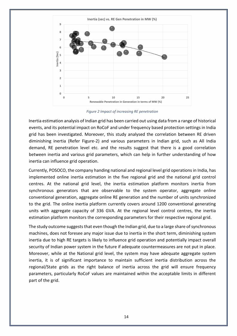
Figure 2 Impact of increasing RE penetration

Inertia estimation analysis of Indian grid has been carried out using data from a range of historical events, and its potential impact on RoCoF and under frequency based protection settings in India grid has been investigated. Moreover, this study analysed the correlation between RE driven diminishing inertia (Refer Figure-2) and various parameters in Indian grid, such as All India demand, RE penetration level etc. and the results suggest that there is a good correlation between inertia and various grid parameters, which can help in further understanding of how inertia can influence grid operation.

Currently, POSOCO, the company handing national and regional level grid operations in India, has implemented online inertia estimation in the five regional grid and the national grid control centres. At the national grid level, the inertia estimation platform monitors inertia from synchronous generators that are observable to the system operator, aggregate online conventional generation, aggregate online RE generation and the number of units synchronized to the grid. The online inertia platform currently covers around 1200 conventional generating units with aggregate capacity of 336 GVA. At the regional level control centres, the inertia estimation platform monitors the corresponding parameters for their respective regional grid.

The study outcome suggests that even though the Indian grid, due to a large share of synchronous machines, does not foresee any major issue due to inertia in the short term, diminishing system inertia due to high RE targets is likely to influence grid operation and potentially impact overall security of Indian power system in the future if adequate countermeasures are not put in place. Moreover, while at the National grid level, the system may have adequate aggregate system inertia, it is of significant importance to maintain sufficient inertia distribution across the regional/State grids as the right balance of inertia across the grid will ensure frequency parameters, particularly RoCoF values are maintained within the acceptable limits in different part of the grid.

0

1

2

3

4

5

6

7

8

9

0 5 10 15 20 25

Iner

tia (S

ec)

Renewable Penetration in Generation in terms of MW (%)

Inertia (sec) vs. RE Gen Penetration in MW (%)

15

Figure 3 Increase in frequency response over the years

The study also assessed the aggregate frequency response observed in the Indian grid for contingencies involving generation or load loss of more than 1000 MW. It was noted that the pursuant to the continuous follow up with the utilities for governor testing and tuning as mandated in the Indian Electricity Grid Code, the combined frequency response has improved despite decrease in inertia.

Based on the study outcome, recommendations, and way forward for accurate inertia estimation and relevant measures/interventions required in Indian grid has been brought out in the report that can be used by various key stakeholders including system regulators, grid operators, generation utilities, policy makers, and OEMs. The key recommendations are summarized below:

0

5000

10000

15000

20000

25000

30000

35000

40000

Jan-

15

Jul-1

5

Dec-

15

Jun-

16

Dec-

16

Jun-

17

Dec-

17

Jun-

18

Dec-

18

Jun-

19

Dec-

19

Jun-

20

Dec-

20

Jun-

21

Dec-

21

ALL INDIA - FREQUENCY RESPONSE CHARACTERISTIC MW/Hz

Note: After Jan 2018, Delta F for FRC calculation is taken from PMU

16

RECOMMENDATIONS

Policy and planning level

1. System inertia to be considered as a critical parameter in planning and operation of the future Indian grid, say beyond 2027, with high penetration of non-synchronous generating resources.

2. Policy initiatives to encourage deployment of synchronous inertia sources, such as synchronous condenser, and hydro generation, besides provisions for synthetic inertia to be provided by non-synchronous resources, for ensuring adequacy of system inertia.

3. Transnational synchronous interconnections leading to a larger footprint would help in increasing system inertia.

4. In a net-zero scenario envisaged by 2070, generation technologies such hydro (including pumped hydro), nuclear, biomass, green hydrogen fired gas turbines, and thermal generation with carbon capture & sequestration need to be kept on the radar in view of inertia requirements.

Regulatory level

5. Technical definitions of system inertia and associated terms to be incorporated in the regulations.

6. Suitable regulatory provisions need to be evolved to harness potential inertial and fast frequency response (FFR) from Renewable Energy sources, other inverter-based resources, including battery energy storage systems.

7. Suitable regulatory provisions and mechanisms to encourage frequency response from demand side resources, including behind-the-meter generation.

Technical level

8. Tools for Inertia estimation, online measurement and forecasting need to be explored.

9. The time window for rate of change of frequency (RoCoF) measurement and RoCoF limits for various protection schemes to be standardized.

10. The Rate of change of frequency (RoCoF), frequency nadir based under frequency load shedding schemes and over frequency settings in the grid need to be revisited periodically.

11. Studies may be initiated to assess the minimum inertia requirement for secure and stable operation of the Indian grid under different operating scenarios.

12. The reference contingency in Indian power system needs to be updated from time to time.

13. Control area frequency response measurement and performance evaluation for frequency events to be strengthened.

14. Governor testing and tuning needs to be pursued at the intra state level also.

15. Synchronous inertia requirements could be considered as one of the constraints in the future Security constrained unit commitment scheme.

17

Indian Power System in Numbers (as on 30-November 2021)

Sl. No. PARTICULARS VALUES

Installed generation capacity of India 1 Generation capacity – Synchronous + Non-synchronous 392 GW

2 Synchronous generation capacity: Coal + Lignite + Gas + Nuclear + Hydro + Biomass 303 GW

3 Non-synchronous generation capacity: Wind + Solar 89 GW 4 Renewable Energy Sources (excluding hydro) 104 GW 5 Non-fossil fuel generation capacity: RES + Hydro + Nuclear 157 GW

Maximum penetration level in India

6 Installed capacity of non-fossil fuel generation 40 % 7 Installed capacity of renewable energy sources (excluding hydro) 26 % 8 Installed capacity of Solar and Wind 23 % 9 Instantaneous MW generation from Solar + Wind 27 %

10 Energy generation from Solar + Wind in a day 16 %

Largest contingency observed in Indian power system 11 Generation loss in Vindhyachal-Sasan complex on 28-May 2020 Loss of 5346 MW 12 Observed change in grid frequency during the contingency 0.48 Hz 13 Observed Nadir frequency during the contingency 49.54 Hz

Typical parameters in Indian power system

14 Highest capacity of single synchronous generating unit (nuclear) 1000 MW 15 Highest capacity of generating station (thermal) 4760 MW 16 Highest solar capacity integrated at single pooling station 2430 MW 17 Highest wind capacity integrated at single pooling station 2305 MW 18 System inertia (assessed from historical data of 2014-2021) 5 - 9 seconds 19 Average Power number (assessed from 2014-2021 historical data) 10000 MW/ Hz 20 Median value of Frequency Response Characteristics 15000 MW/Hz 21 Time to reach Nadir/Zenith frequency (Dec 2017 to Jun 2021) 9-14 seconds 22 Observed load damping of frequency sensitive load 2-5%

Operating standards

23 Operating frequency band as per Indian Electricity Grid Code 49.90 - 50.05 Hz

24 Reference contingency (IEGC 2020 expert committee report) for defense plans Loss of 4500 MW

25 Nadir frequency for reference contingency (as per simulations) 49.55 Hz

26 Quasi steady state frequency for reference contingency (as per simulations) Assuming Frequency Response Characteristics of 15500 MW/Hz

49.71 Hz

27 Setting of 1st stage Automatic Under frequency-based Load shedding Scheme 49.4 Hz

28 Setting of 1st Stage of df/dt (Rate of change of frequency-based) load shedding

- 0.1 Hz/sec, 49.9 Hz

18

Abbreviations and Symbols AC Alternating Current

DC Direct Current

COI Centre of Inertia

F Frequency

FFR Fast Frequency Response

GW Gigawatt

GWh Gigawatt-hour

GW•s Gigawatt-second

IBR Inverter-Based Resource

kW Kilowatt

kWh Kilowatt-hour

LR Load Response

MW Megawatt

MWh Megawatt-hour

MW•s Megawatt-second

NLDC National Load Dispatch Centre

PMU Phasor Measurement Unit

PV Photovoltaics

RLDC Regional Load Dispatch Centre

RE Renewable Energy

RoCoF Rate of Change of Frequency

SCADA Supervisory Control and Data Acquisition

UFLS Underfrequency Load Shedding

19

Chapter 1: Introduction

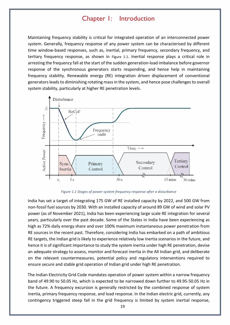
Maintaining frequency stability is critical for integrated operation of an interconnected power system. Generally, frequency response of any power system can be characterised by different time window-based responses, such as, inertial, primary frequency, secondary frequency, and tertiary frequency response, as shown in Figure 1.1. Inertial response plays a critical role in arresting the frequency fall at the start of the sudden generation-load imbalance before governor response of the synchronous generators starts responding, and hence help in maintaining frequency stability. Renewable energy (RE) integration driven displacement of conventional generators leads to diminishing rotating mass in the system, and hence pose challenges to overall system stability, particularly at higher RE penetration levels.

Figure 1.1 Stages of power system frequency response after a disturbance

India has set a target of integrating 175 GW of RE installed capacity by 2022, and 500 GW from non-fossil fuel sources by 2030. With an installed capacity of around 89 GW of wind and solar PV power (as of November 2021), India has been experiencing large scale RE integration for several years, particularly over the past decade. Some of the States in India have been experiencing as high as 72% daily energy share and over 100% maximum instantaneous power penetration from RE sources in the recent past. Therefore, considering India has embarked on a path of ambitious RE targets, the Indian grid is likely to experience relatively low inertia scenarios in the future, and hence it is of significant importance to study the system inertia under high RE penetration, devise an adequate strategy to assess, monitor and forecast inertia in the All Indian grid, and deliberate on the relevant countermeasures, potential policy and regulatory interventions required to ensure secure and stable grid operation of Indian grid under high RE penetration.

The Indian Electricity Grid Code mandates operation of power system within a narrow frequency band of 49.90 to 50.05 Hz, which is expected to be narrowed down further to 49.95-50.05 Hz in the future. A frequency excursion is generally restricted by the combined response of system inertia, primary frequency response, and load response. In the Indian electric grid, currently, any contingency triggered steep fall in the grid frequency is limited by system inertial response,

20

primary frequency response and further controlled by automatic Under Frequency Relay based load shedding (AUFLS), which has its first stage at 49.4 Hz and the rate of change of frequency-based load shedding which has its first stage set at 49.9 Hz and 0.1 Hz per second. The most credible reference contingency presently considered in the Indian power system is the outage of the largest power plant with around 4500 MW generation capacity.

In the thrust towards an intelligent and smart grid, over the past decade, Indian power system has been experiencing Wide Area Measurement Systems (WAMS) implementation with data from more than 1500 Phasor Measurement Units (PMU) being fed to the control centres. The high-resolution data provided by the PMUs installed across the Indian power system is currently being used for monitoring and analysis applications. The events associated with high rate of change of frequency (RoCoF) are monitored using PMUs. The raw data obtained from PMUs is filtered through statistical methods, which is used to estimate generation-load imbalance for each event with high RoCoF. The frequency response characteristics of the various control areas are also assessed as per the procedure approved by the Central Electricity Regulatory Commission. The aggregate frequency response characteristic (FRC) of the Indian grid is approx. 15 GW/Hz.

The frequency profile of three identified generation loss events experienced in Indian grid are summarised below:

i. On 12th March 2014 at 19:22 hrs, the Indian grid experienced an unplanned outage of CGPL power plant at Mundra that was triggered by tripping of all the power evacuating lines from the plant, which resulted in a generation loss of 4030 MW (CGPL: 3750 MW + 280 MW wind generation in the vicinity). The grid frequency due to the generation loss event dropped by 0.67 Hz (from 49.95 Hz to 49.285 Hz). The under-frequency event led to the a system load loss of 1110 MW which includes 960 MW due to df/dt based load shedding (Gujarat: 630 MW + Maharashtra: 330 MW) and 150 MW due to reduction in export to Bangladesh due to SPS operation, as shown in Figure 1.2 (The 1st stage of under frequency load shedding was triggered at 49.2 Hz).

Figure 1.2 Frequency response during 12 March 2014 event

ii. On 23rd April 2018 at 10:42 hrs, during the testing of a circuit breaker at 765/400kV Kotra S/S, the substation experienced single line to ground (B phase to earth) fault. This event led

21

to tripping of generators at RKM, SKS, Lara, DB Power, KSK and KWPCL stations resulting in a total generation loss of 3089 MW. The grid frequency initially dropped by 0.30 Hz (from 50.01 Hz to 49.71 Hz) followed by further drop of additional 0.1 Hz (total of 0.4 Hz, from 50.01 Hz to 49. 61 Hz), as can be observed from the event frequency response shown in Figure 1.3.

Figure 1.3 Frequency response during 23 April 2018 event

iii. On 28th May 2020, inclement weather resulted in tripping of multiple transmission lines at 765 kV Satna, Sasan and Vindhyachal Pooling stations. Consequently, there was an aggregate loss of 5346 MW at Sasan, Vindhyachal NTPC Stage IV & V, and Rihand Stage III generating stations. It resulted in frequency drop of 0.48 Hz (50.02 Hz to 49.54 Hz) as shown in Figure 1.4.

Figure 1.4 Frequency response during 28 May 2020 event

This report attempts to analyse the initial frequency response over the first few seconds from the onset of the frequency disturbance, covering inertial response and primary frequency response windows. It is important to note that the overall inertial response offered by the system to a frequency disturbance primarily includes the response from generator and load inertia. Other grid elements and inverter-based resources (IBRs) can also contribute to the overall inertial

22

response. Moreover, this report also dwells upon the system inertia monitoring and its online as well as offline assessment with the help of measurements available in the load despatch centres.

Chapter-2 presents a theoretical concept of inertia to provide an understanding of the dynamic frequency behaviour of the power system. Chapter-3 covers a survey of international best practices in the field of power system inertia measurement and estimation. The inferences have been drawn from the practices in some of the major power systems of the world.

Chapter-4 describes the inertia of synchronous generating units in the Indian power system, where inertia contribution of each category of generation has been discussed. Chapter-5 of the report describes the measurement-based inertia estimation topic, while the corresponding analysis of inertia estimation for Indian power system is provided in Chapter-6. Chapter-7 describes the implementation of inertia estimation platform and its visualisation as implemented in control room SCADA/EMS. Chapter-8 details the status of primary frequency response in Indian power system and its monitoring. Chapter-9 covers inertia trends due to RE penetration and the all-India simulation model and analysis. Chapter-10 summarises the report and provides the recommendations and way forward for the key stakeholders, including policy makers and regulators.

23

Chapter 2: Inertia: Theoretical Background

This chapter describes the fundamental concept of inertia/ kinetic energy of a power system and its importance in frequency control during sudden generation-load imbalances.

2.1 Concept of Inertia The concept of inertia is a fundamental concept of classical mechanics. The inertia of a physical object is defined as the property by virtue of which it resists any change in the state of relative rest or of a uniform linear (or rotational) motion. The change can include the change in the magnitude or direction of its velocity.

According to Newton's second law of motion, the acceleration ‘�⃗�𝑎’ of an object produced by an external force is directly proportional to the magnitude of the force ‘ �⃗�𝐹’ and inversely proportional to the mass `𝑚𝑚’ of the object.

�⃗�𝑎 = �⃗�𝐹/𝑚𝑚 …...………. (2.1)

Here, for the case of linear motion, the physical mass of the object is the measure of inertia. The larger the mass of the object, the lower will be the acceleration produced, thus yielding a greater resistance to the change in its state of motion, and hence, has a higher value of inertia.

In the case of rotational motion, if the shape of the body remains unchanged, Newton's second law can be written in terms of the applied torque 𝜏𝜏 and angular acceleration 𝛼𝛼 around a principal axis as,

𝜏𝜏 = 𝐼𝐼 ∗ 𝛼𝛼 …...………. (2.2)

Here, 𝐼𝐼 represents the moment of inertia of a rigid body, which is analogous to the mass 𝑚𝑚 in the case of linear motion, giving a measure of the inertia for the mass in rotational motion. The moment of inertia depends on both the mass 𝑚𝑚 of the body and its geometry or shape, as defined by the distance 𝑟𝑟 to the axis of rotation.

𝐼𝐼 = ∑𝑚𝑚𝑖𝑖𝑟𝑟𝑖𝑖2 …...………. (2.3)

The moment of inertia for a rotational mass is of interest for assessing power system inertia, as it can represent the rotating mass of a synchronous machine that delivers the system inertial response. In regard to power system study, and also used in the remainder of this report, the moment of inertia of a synchronous machine is represented by the symbol 𝐽𝐽.

24

2.2 Inertia of power system Inertia of a conventional power system primarily comprises of the energy stored in the rotating mass of synchronous generators, with a partial contribution from frequency sensitive load. Since the speed of rotating synchronous generators and grid frequency is magnetically locked, the rotational energy stored in the synchronous machines, generally known as kinetic energy resists any sudden change in the grid frequency from its nominal/steady state value by releasing stored kinetic energy to the grid. Frequency of an AC grid is required to be maintained within a narrow band. In India, the grid operator is currently required to maintain the system frequency within the band of 49.90 - 50.05 Hz, which is expected to be narrowed down further in future. One of the fundamental requirements for stable operation of synchronous AC grid is that power generation and consumption (load and losses) is balanced at every instant of real time operation, and it is this kinetic energy of rotating synchronous machines (inertia) that helps the grid to maintain generation-consumption balance in the initial few seconds from the onset of a credible contingency, such as, a generation tripping or loss of load. A simple understanding of power system inertia can be derived from a water tank analogy shown in Figure 2.1. The quantity of water stored in the tank represents aggregate kinetic energy stored in a conventional power system, and the level of the stored water represents grid frequency. For example, in case of a generation outage due to a fault induced tripping, the system will experience an instant shortfall of generation (water flow input), as additional generation from online units cannot be brought in instantly due to delay in governor response (typically 3-4 sec) followed by ramp up rate limits of the generating units. Therefore, initially at the start of the generation outage (shortfall of water input), to maintain generation and load balance, the stored rotational energy (stored water in the tank) caters to the additional net load seen by the system, and helps in arresting the fall of frequency and consequently the maximum frequency deviation before the generator governor response is activated. Therefore, maintaining an adequate level of inertia (stored water in tank) in rotating synchronous machine-based power system is critical for frequency stability of the system. The amount of inertia (releasable kinetic energy) available in a given operating scenario determines the time rate at which frequency will fall initially, which does not only influence the amount of load shedding (hence reliability) but also vulnerability of the system to a potential blackout in the worst case scenario.

Inertia of a synchronous machine and hence power system, as described in this section later, can be quantified in terms of inertia constant ‘H’ measured in seconds. The inertia constant of a synchronous machine can be theoretically defined as the time in seconds for which the machine can supply its rated power only form its stored kinetic energy in the rotor. Inertia constant of a synchronous generating unit varies typically between 2-10 seconds, depending on the type and size of the generating unit. Similarly, for a conventional power system, the aggregate equivalent inertia constant can be defined as the time in seconds for which the system can supply its aggregate online rated generation from its aggregate stored kinetic energy only. However, practically, the time for which a synchronous generator or the power system can supply power only from its stored kinetic energy is limited by the frequency and rate of change of frequency based protection settings of load shedding schemes and generator protection. Renewable Energy (RE) integration driven displacement of conventional generation results in diminishing of system inertia due to displacement of rotating mass in the system, thereby, necessitating assessment and monitoring of system inertia, and plan the system inertia adequacy accordingly.

25

Figure 2.1 Power system inertia and water tank analogy

The concept of inertia in a synchronous machine can be understood through the mathematical model proposed in [1]. In this model, the stability of a single synchronous machine connected to an infinite bus is analysed.

The assumptions made to represent a synchronous generator mathematically by a classical model are summarised below:

1. The exciter dynamics are not considered, and the field current is assumed to be constant so that the stator induced voltage is always constant during the period of study.

2. The effect of damper windings present in the rotor of the synchronous generators is neglected.

3. The input mechanical power to the generator is assumed to be constant during the period of the study.

4. The saliency of the generator is neglected; that is, the generator is assumed to be of cylindrical type rotor.

The assumptions stated above make the representation of synchronous generator simple for the inertia related analysis. Assumptions 1 and 2 ignores the dynamics of exciter, damper windings, and rotor windings. Assumption 3 leads to neglecting the dynamics of turbine and turbine speed governor. Assumption 3 is justified as the change in the mechanical input power takes more time due to the involvement of mechanical systems, whereas the electrical power output can change instantaneously.

A generator connected to an infinite bus through a transformer and a transmission line, commonly known as Single Machine Infinite Bus (SMIB) system, as shown in Figure 2.2, is used for a more detailed analysis and understanding. Since the resistance of the synchronous generator stator, transformer, and transmission line are relatively negligible as compared to the

26

corresponding reactance value, the resistance of all three elements is ignored. The infinite bus represents the rest of the external grid, where the voltage magnitude and frequency are held constant. The infinite bus voltage angle is taken as the reference angle, with its angle taken as zero. The generator internal voltage angle δ is defined with respect to the infinite bus voltage angle.

Table 2.1 defines various symbols and parameters used in the SMIB analysis.

Table 2.1 Parameters for Single Machine Infinite Bus model

𝐸𝐸∠𝛿𝛿 Internal emf phasor of the synchronous generator behind the transient reactance 𝑋𝑋𝑑𝑑

/

𝑉𝑉𝑇𝑇∠𝜃𝜃𝑇𝑇 Terminal voltage phasor of the synchronous generator

𝑋𝑋𝑇𝑇 Transformer reactance

𝑋𝑋𝐿𝐿 Line reactance

𝑉𝑉∞∠00 Infinite bus voltage phasor

δ Generator internal voltage/load angle

𝑃𝑃𝑚𝑚 Input mechanical power to the synchronous generator

𝑃𝑃𝑒𝑒 Generator output electrical power

𝐻𝐻 Inertia constant of the generator

𝐻𝐻∞ Inertia constant of the infinite bus.

Figure 2.2 Impedance diagram of the single machine infinite bus system

The maximum active power output of the synchronous generator that can be potentially transferred to the infinite bus is given as

𝑃𝑃𝑚𝑚𝑚𝑚𝑚𝑚 =𝐸𝐸𝑉𝑉∞

𝑋𝑋𝑑𝑑′ + 𝑋𝑋𝑇𝑇 + 𝑋𝑋𝐿𝐿

…...………. (2.4)

The electrical power output of the synchronous generator can be represented as

𝑃𝑃𝑒𝑒 = 𝑃𝑃𝑚𝑚𝑚𝑚𝑚𝑚 sin𝛿𝛿 …...………. (2.5)

27

The prime mover provides mechanical power to the generator rotor and in turn, the generator converts the mechanical energy into electrical energy. The dynamics of the generator electromechanical system can be represented as

𝐽𝐽𝑑𝑑2𝛿𝛿𝑚𝑚𝑑𝑑𝑡𝑡2

= 𝑇𝑇𝑚𝑚 − 𝑇𝑇𝑒𝑒 …...………. (2.6)

where 𝐽𝐽 is the moment of inertia of the rotating machine in 𝑘𝑘𝑘𝑘.𝑚𝑚2. The mechanical input torque due to the prime mover is represented as 𝑇𝑇𝑚𝑚 in 𝑁𝑁.𝑚𝑚 and the electrical torque acting against the mechanical input torque, is represented by 𝑇𝑇𝑒𝑒 in 𝑁𝑁.𝑚𝑚 . Where, 𝛿𝛿𝑚𝑚 is the mechanical angle between the rotor field axis and the reference axis rotating synchronously at 𝜔𝜔𝑚𝑚𝑚𝑚.

Equation (2.6) can be further rearranged and written as given below

𝐻𝐻𝑑𝑑2𝛿𝛿𝑚𝑚𝑑𝑑𝑡𝑡2 =

1

2𝜔𝜔𝑚𝑚𝑚𝑚(𝑃𝑃𝑚𝑚 − 𝑃𝑃𝑒𝑒)

…...………. (2.7)

Where, 𝐻𝐻 is termed as the inertia constant of the generator expressed in seconds, and 𝑆𝑆𝐵𝐵 is the rated apparent power of the generator. The inertia constant 𝐻𝐻in eq. (2.7) can be expressed as

𝐻𝐻 =12𝐽𝐽𝜔𝜔𝑚𝑚𝑚𝑚2 𝑆𝑆𝐵𝐵

𝑚𝑚 …...………. (2.8)

Inertia constant is a preferred term to specify the inertia of a synchronous machine, which represents the time (in seconds) that the energy stored in the rotating mass of the machine can supply a load at its rated power.

Inertia of a power system can be broadly defined as the resistance offered by the system to a change in frequency following a generation-load imbalance by providing inertial response from synchronous machines, load side response, inertial response from IBRs (if employed), and other grid elements/equipment. The predominant source of inertia in conventional systems is synchronous generators, followed by the load side response.

A large power system consists of several synchronous machines operating in parallel and connected through the transmission and distribution system. The aggregate equivalent inertia of a power system can be calculated using the inertia constants and rated apparent powers of individual synchronous machines as follows:

𝐻𝐻𝑚𝑚𝑠𝑠𝑚𝑚 =∑ 𝑆𝑆𝑖𝑖 ∗ 𝐻𝐻𝑖𝑖𝑛𝑛𝑖𝑖=1∑ 𝑆𝑆𝑖𝑖𝑛𝑛𝑖𝑖=1

…...………. (2.9)

Where 𝑆𝑆𝑖𝑖 is the rated apparent power of generator 𝑖𝑖 [VA] and 𝐻𝐻𝑖𝑖 is the inertia constant of turbine-generator 𝑖𝑖 [s] and 𝑛𝑛 is the number of synchronous generators.

It is often more convenient to calculate the kinetic energy stored in synchronously rotating masses of the system in megawatt seconds (MWs). Therefore, Equation (2.9) can be written as:

28

𝐸𝐸𝑘𝑘,𝑚𝑚𝑠𝑠𝑚𝑚 = �(𝑆𝑆𝑖𝑖 ∗ 𝐻𝐻𝑖𝑖

𝑛𝑛

𝑖𝑖=1

)

…...………. (2.10)

The moment of inertia of a conventional generator represents the equivalent inertia of the drive train of the power plant. The drive train system of a power plant usually consists of several masses rotating on the same shaft. In a coal-based power plant, there are generally three stages of turbines: high-pressure (HP), intermediate pressure (IP), and low pressure (LP) steam turbine, as shown in Figure 2.3. The entire turbine shaft rotates at the same speed, with the moment of inertia as the sum of the individual moments of inertia for each mass. The complete turbine system has various torsional modes depending on the relative inertia and the damping of each rotor mass together with the shaft sections connecting each mass. The torsional modes are sub synchronous in nature, and therefore for synchronous frequency operation, they are neglected, and complete mass, including the generator rotor, is considered as a single equivalent mass and inertia. In terms of the block diagram, it can be understood that sum of inertia of all the blocks is the inertia of the machine.

Figure 2.3 Drive train of a thermal power plant with three pressure stages.

It is, however, important to note that due to the generator speed limits and grid frequency limits, a generator can release only a part of its stored energy to the grid. In an alternator, the rotational speed depends on the number of pole pairs and the frequency of EMF generated in the armature.

2.3 Inertial response in power system observed through grid frequency The modern power system is a dynamically changing system with constantly varying electricity consumption and a varying mix of sources that cater to the total demand. During its different dynamic operating conditions, the system has to be resilient enough to maintain stability under conditions of transient disturbances. Small disturbances in the form of load changes occur continuously, and the system adjusts itself accordingly without much impact on the system stability. However, for large power imbalances, the system frequency can deviate much further from the nominal operating range.

For a sudden generation deficit, such as following a trip of a generation unit, the instantaneous imbalance in total generation and load will be initially delivered from the inertial response of all synchronously connected rotating masses. The rotational energy stored in the generators is released to the grid through the inertial response, thereby reducing the speed of the rotors and consequently reducing the system frequency. The initial RoCoF, which is also its maximum value

29

for a given disturbance and operating point depends on the size of the active power disturbance and the system inertia.

The electromechanical dynamics of a synchronous generator can be described using the motion equation of its rotating mass (the swing equation, eq. 2.7):

2𝐻𝐻𝑖𝑖𝑓𝑓0

𝑑𝑑𝑓𝑓𝑖𝑖𝑑𝑑𝑡𝑡

=𝑃𝑃𝑚𝑚𝑖𝑖 − 𝑃𝑃𝑒𝑒𝑖𝑖

𝑆𝑆𝑖𝑖

…...………. (2.11)

Equation (2.11) shows that an imbalance between the mechanical and electrical power results in a frequency derivative. Thus, the RoCoF at the instant of the disturbance is determined by the size of the imbalance (𝑃𝑃𝑚𝑚 − 𝑃𝑃𝑒𝑒) and inertia of the turbine generator.

In a real power system, a large number of generating units, which are spread through a vast area, deliver power to the loads via the electrical network. Thus, when an imbalance in the system arises, frequency is not uniform throughout the system. Hence, for a system of 𝑁𝑁 synchronous machines, the swing equation can be written as,

2𝐻𝐻𝑚𝑚𝑠𝑠𝑚𝑚𝑓𝑓0

𝑑𝑑𝑓𝑓𝐶𝐶𝐶𝐶𝐶𝐶𝑑𝑑𝑡𝑡

=𝑃𝑃𝑚𝑚 − 𝑃𝑃𝑒𝑒

𝑆𝑆

…...………. (2.12)

Where, 𝑓𝑓𝐶𝐶𝐶𝐶𝐶𝐶 is the centre of inertia frequency of the system and is defined as,

𝑓𝑓𝐶𝐶𝐶𝐶𝐶𝐶 =∑ 𝑓𝑓𝑖𝑖𝐻𝐻𝑖𝑖𝑁𝑁𝑖𝑖−1∑ 𝐻𝐻𝑖𝑖𝑁𝑁𝑖𝑖−1

…...………. (2.13)

Where the inertia constant 𝐻𝐻𝑖𝑖 of each generator is expressed at a common 𝑉𝑉𝑉𝑉 base.

Figure 2.4 shows the behaviour of frequency after a generation loss event with varying amounts of kinetic energy in the system [2]. It shows that higher kinetic energy in the system results in slower frequency fall and higher maximum frequency deviation. The dotted line, which is the tangent at the beginning of the disturbance, shows the variation in the RoCoF.

Figure 2.4 Impact of diminishing inertia on system frequency response [2]

Several parameters/matrices of the frequency deviation curve can be defined in order to assess the impact of system inertia and stability after a major disturbance. Figure 2.5 provides the different frequency response parameters, which include the start time of disturbance, frequency before the disturbance, minimum or maximum instantaneous frequency, maximum frequency deviation, and time to reach maximum instantaneous frequency deviation.

30

For accurate inertia estimation, determining the accurate start time of a frequency disturbance is critical, and that may not be straightforward in several cases. One way to do this is to examine 𝑑𝑑𝑓𝑓/𝑑𝑑𝑡𝑡, known as the RoCoF. The start time of disturbance is taken as the time when the absolute value of the rate of change of frequency obtained by signal filtering exceeds a set threshold. This threshold setpoint is chosen after careful observations and performing empirical analysis. The start time is very important as further parameters are dependent on the correct start time. In the Nordic inertia study, the start of the frequency disturbance is taken as the instant at which absolute value of the RoCoF, calculated from the filtered frequency, exceeds 0.035 Hz/s.

The authors in the research paper [3] have proposed that detrended fluctuation analysis can be used for detecting the start time of the event for inertia estimation. The study calculates the fluctuation in the frequency curve over a specific time period (e.g., 1 sec taken for the GB system). The start of the disturbance is then determined when the fluctuation exceeds a predetermined value. The method claims to prevent the detection of frequency events such as gradual frequency changes due to secondary controller action or multiple successive frequency events that are not suitable for inertia estimation.

The minimum (𝑓𝑓𝑛𝑛𝑚𝑚𝑑𝑑𝑖𝑖𝑛𝑛 ) or maximum instantaneous frequency (𝑓𝑓𝑧𝑧𝑒𝑒𝑛𝑛𝑖𝑖𝑧𝑧ℎ), also known as nadir or zenith frequency, is defined as the lowest value of underfrequency or the highest value of over frequency during a disturbance, depending on whether there was a net loss of generation or load. This value is highly dependent on the size of the net loss of generation/load, the frequency at the time of the start of disturbance as well as the inertia of the system. The time at which the frequency reaches 𝑓𝑓𝑛𝑛𝑚𝑚𝑑𝑑𝑖𝑖𝑛𝑛 is defined as 𝑡𝑡𝑛𝑛𝑚𝑚𝑑𝑑𝑖𝑖𝑛𝑛. For the disturbance in Figure 2.5, which is a loss of generation unit, the minimum instantaneous frequency 𝑓𝑓𝑛𝑛𝑚𝑚𝑑𝑑𝑖𝑖𝑛𝑛 = 49.8 Hz occurs at 𝑡𝑡𝑛𝑛𝑚𝑚𝑑𝑑𝑖𝑖𝑛𝑛 =11.4𝑚𝑚.

.

Figure 2.5 Frequency response indicators

The change in frequency, ∆𝑓𝑓, is defined as the difference between the minimum or maximum instantaneous frequency deviation and the frequency at the start of the disturbance.

∆𝑓𝑓 = |𝑓𝑓𝑛𝑛𝑚𝑚𝑑𝑑𝑖𝑖𝑛𝑛 − 𝑓𝑓𝑚𝑚𝑧𝑧𝑚𝑚𝑛𝑛𝑧𝑧| = |49.805 − 49.885| = 0.08 𝐻𝐻𝐻𝐻

31

In the same way, the time to reach the maximum frequency deviation is calculated.

∆𝑡𝑡 = |𝑡𝑡𝑛𝑛𝑚𝑚𝑑𝑑𝑖𝑖𝑛𝑛 − 𝑡𝑡𝑚𝑚𝑧𝑧𝑚𝑚𝑛𝑛𝑧𝑧| = |11.4 − 1.2| = 10.2 𝑚𝑚

For the disturbance shown in Figure 2.4, the change in frequency is ∆𝑓𝑓 = 0.08 𝐻𝐻𝐻𝐻 and the time to reach the maximum frequency deviation is ∆𝑡𝑡 = 10.2 𝑚𝑚 . This deviation in frequency is an important indicator to assess the value of frequency nadir. The under-frequency load shedding can be set by knowing this value and sufficient reserves can be maintained to maintain stability during any credible contingency. This simple understanding provides the required inputs for the estimation of inertia using the swing equation. Along with the inertia, the performance of the primary response can also be evaluated, and relevant feedback to planners can be given regarding the expected minimum/maximum frequency for any credible contingency. Seasonal, as well as diurnal variations in inertia and frequency response can also be recorded.

2.4 Challenges in power system operation under low inertia With the expected decrease in inertia due to RE driven displacement of conventional generation, it is important to assess the influence of reduced inertia on the power system dynamics, and determine the relevance of inertia in the stability, reliability and operation of the power system. The time period of power system dynamics ranges from microseconds/milliseconds to seconds. The slower electromagnetic phenomenon occurring in power system take place in the frame of milliseconds to seconds. The inertia comes into picture in the timeframe of few seconds and plays an important role in electromechanical phenomenon post a disturbance. Some of the main challenges with respect to the different forms of power system stability issues with lower synchronous machines in the grid are discussed in this section.

i. Impact on frequency stability: Diminishing synchronous inertia leads to higher RoCoF following a credible contingency in the system, thereby posing challenges in maintaining maximum RoCoF and frequency nadir/zenith within the acceptable limits. Moreover, the aggregate governor response of the system that declines due to RE penetration can also pose issues in the primary frequency control. While inverter interfaced RE sources can technically support the grid during overfrequency events by reducing their output, they would need to be curtailed in advance for frequency support in underfrequency events. Frequency support for underfrequency may not be feasible due to economical, policy and regulatory reasons, except for forced RE generation curtailment cases due to network issues (stability/congestion etc.). The frequency operating range is defined in the grid standards and sets a certain tolerance around the nominal frequency within which generators should remain connected to the transmission grid. In Indian power system, Central Electricity Authority (Technical Standards for Connectivity to the Grid) Regulations mention that “The generating unit shall be capable of operating in the frequency range 47.5 to 52 Hz and be able to deliver rated output in the frequency range of 49.5 Hz to 50.5 Hz”. The Distributed energy sources are intended to trip after 200 msec when frequency goes below 47.5 Hz or rises above 50.5 Hz. The frequency excursion for an extended period can cause cascaded trappings in the system.

ii. Transient stability: The reduction of power system inertia reduces its ability to damp out the oscillations. The effect is more pronounced when there are large perturbations in steady

32

state conditions of the system. The Critical clearing time (CCT) of faults is also decreased due to reduction in inertia. The reduction in CCT causes elements to be disconnected in cascade causing insecure conditions in power system. However, transient stability performance will also largely depend on the control employed in the IBRs and grid code regulation in place. Some of the related studies have concluded that transient stability issues can be tackled by an adequate system planning and adaptive grid operation practices.

iii. Impact on Power system protection: The reliability of power system lies to a great extent on the accurate operation of power system protection. The reduced inertia is one of the reasons that result in high Rate of Change of Frequency (RoCoF) values post any contingency. The system protection schemes are devised in a power system to handle the extreme events of RoCoF and low frequency. The Under-Frequency Load Shedding (UFLS) schemes are deployed to operate when frequency reaches below a certain threshold. UFLS protection is activated only after the frequency breache of the set limits is detected, which involves frequency measurement and relay activation delay. High RoCoF values in such cases can result inaccurate operation of UFLS schemes or potentially the system collapse in the worst case scenario. Moreover, RoCoF based protection is likely to be activated more often under low system inertia.

iv. Impact on Short Circuit capacity of the system: The synchronous machines are capable of injecting around 7-8 times its nominal current almost instantaneously for a dead short circuit at its terminal. Such instantaneous reactive power injection helps the system voltage recovery following fault clearance and, therefore, improves its transient stability. Moreover, the protection schemes in conventional systems are designed based on the short circuit current injection of synchronous generators. However, RE integration, particularly at large scale results in displacement of conventional generators, thereby leading to decreased short circuit capacity and reactive power reserve in the system, as the short circuit current capability of IBRs is significantly low (typically 1-1.6 per unit). The implemented power system protection scheme relies on a system with high capability of short-circuit current injection, however with the decrease of this capability, this scheme needs to be continuously monitored and evaluated to avoid any maloperation of protection scheme.

v. Impact on small signal stability: Power system experiences mainly four types of power oscillation which include, intra plant (2-3 Hz), local mode (1-2 Hz), inter-area (1 Hz or less) and torsional mode oscillations (10-46 Hz). For a secure system, all the oscillations should be adequately damped under all the scenarios. The system damping level may be influenced by RE penetration level depending on the generation technology (type of WTG, solar PV inverter). For example, RE driven displacement of synchronous generators is likely to decrease damping effect due decreased number of power system stabilisers equipped with the displaced generators. Moreover, the interaction between IBRs and synchronous machines may affect the damping torque in the system, hence influencing the overall system damping performance. However, some relevant studies have concluded that some of RE generation technology, for example, type 1 and type 3 WTGs improved the system damping response more than synchronous generators. Therefore, no clear and generalised conclusion can be drawn on the impact of RE penetration on power oscillation damping.

33

vi. Impact on admissible frequency range and RoCoF: The frequency operating range is defined in the grid standards and sets a certain tolerance around the nominal frequency within which generators should remain connected to the transmission grid. The frequency excursion for an extended period can cause cascaded trippings in the system. In addition to the admissible frequency range, it is important to analyse the maximum RoCoF that can be permitted in the power system. RoCoF is often used in combination with the frequency change to trigger load shedding relays as it provides a more selective and/or faster operation. The determination of a maximum RoCoF limit for an electrical power system means to determine the “maximum stress” that it can sustain and survive. The target minimum inertia to be ensured in the system can be determined using reference contingency, UFLS scheme first stage threshold frequency and delays in action of UFLS/ROCOF relays. However, low inertia system scenarios would imply higher maximum RoCoF values will be experienced by the system. Therefore, settings of RoCoF and frequency based protection schemes may need to be revisited to explore possibility of relaxing/modifying such threshold limits currently being used for the protection schemes.

In view of the above discussion, it can be concluded that a reduction in system inertia affects the power system stability and results in increased RoCoF and deteriorated frequency nadir for the same power imbalance compared to conventional system. The minimum inertia for secure power system operation is majorly dependent on RoCoF withstand values of the system. High maximum RoCoF values following an event increases the risk of the system frequency falling to load-shedding thresholds. Therefore, system inertia is one of the important parameters along with primary frequency control to determine the maximum time delay for governor and prime movers to react and control the frequency decline.

2.5 Classification of inertia estimation methods In recent years, there has been a significant focus on accurately estimating system inertia, which can be primarily attributed to diminishing inertia due to RE integration. The inertia estimation methods reported in the literature can be broadly classified based on the time frame of estimation and target level of the inertia. Based on the time frame of estimation, the estimation methods can be classified into offline methods, online or real-time methods, and forecasting methods. On the other hand, based on the target level of estimated inertia, estimation methods are classified as system level, regional level, inertia of a synchronous generator, power electronics interfaced source (or embedded generation), and demand levels. Figure 2.6 shows the overall classification of the inertia estimation methods.

34

Figure 2.6 Classification of inertia estimation methods

2.5.1 Offline Estimation Methods As the name suggests, inertia estimation is carried out using the historical frequency and power response data measured during large disturbances in the power system. With the measured size of the disturbance and the value of the initial RoCoF calculated from the measured frequency, system inertia is estimated using the swing equation. Inoue et al. first proposed the offline post-mortem estimation method [4] to estimate the inertia of Japan's power system. Since then, several other studies have been published in the literature that estimates system inertia using the offline method. These methods can be further sub classified into system-level, regional level, synchronous generation, converter interfaced generation, and demand-side/load estimation.

Some of the main challenges in offline inertia estimation include (i) size of active power disturbance, time of occurrence, and location of the events, (ii) frequency measurement throughout the power system since the frequency change following a frequency event vary from location to location, (iii) processing the measured frequency for eliminating unwanted oscillations present by using appropriate filters so that the RoCoF can be calculated correctly.

One of the disadvantages of this method is that the estimated inertia is not a real-time value and is discrete. The estimated inertia values cannot be directly used for real-time decision-making as the value may continually change depending on the number of online synchronous generators and loading conditions. In the offline estimation methods, where inertia is calculated using the swing equation, the time window considered for RoCoF calculation also influences the accuracy of the estimate. Moreover, the method is less reliable when a significant amount of PE-based sources are embedded in the system along with virtual inertia provision. The primary reason is that the released inertial response from these PE-based sources during disturbances is not identical/comparable to the response from synchronous generators.

2.5.2 Online or real-time inertia estimation methods In contrast to the post-mortem analysis based on historical data, the online estimation approaches estimate inertia online by utilizing real-time measurements. The online estimation method can be further sub-classified into discrete and continuous methods. The estimation methods can also be categorised according to the domain in which the inertia is estimated, i.e., time-series, Laplace domain, and modal-domain based methods. Time series methods are concerned with the use of measured time series data and estimation of inertia with the simplified

35

swing equation. While for the Laplace domain method, transfer functions models are used for a system-identification based approach of inertia estimation. Lastly, the modal domain methods estimate inertia based on modal analysis of the inter-area oscillations captured during an active power disturbance. Figure 2.7 provides the overall sub-classifications of literature under the online inertia estimation method.

Figure 2.7 Sub classification of online inertia estimation methods

Discrete estimation methods

The discrete methods provide inertia estimates close to real-time, using measured frequency transients during large disturbances happening in the system. This process of calculating the inertia is similar to that of the offline estimation which is based on a linearized swing equation. The challenges in this type of inertia estimation method include detection of an appropriate disturbance online under the influence of oscillations present in the frequency data and estimation of the actual size of the disturbance from the available measurements. Moreover, as the name suggest, such methods rely on large naturally occurring disturbances in the system that will be appropriate for the estimation algorithm.

The use of moving average filtering methods to detect the disturbance, online is considered to be more realistic RoCoF calculation. Moreover, assuming that the mechanical power output of a generator remains unaltered at the instant of a disturbance, the difference in electrical power output of a generator just after the instant of disturbance can be estimated as the disturbance size. Also, at a regional level, the changes in inter-area tie-line flow during disturbances have also been taken as an imbalance for estimating area inertia.

Continuous estimation methods

In these methods, the inertia of the power system is estimated continuously with a better temporal resolution, using measured frequency and power measurement data during normal operating conditions. Various approaches, such as model-analysis based approaches using ambient data measurement, and the probing signal-injection based method, have been used to estimate system inertia.

Even though continuous estimation during normal conditions will be ideal, the accuracy and reliability of these methods are still a major issue. A notable change in frequency for small power change in normal operating conditions is difficult to obtain since other oscillations of similar magnitude can be present in the measured data. Also, concerns of power quality issues due to injected micro-disturbance signal make these methods less convincing. Furthermore, these

36

methods are not validated under lower inertia conditions and with a significant level of virtual inertia present in the power system.

2.5.3 Estimation of expected inertia by forecasting Forecasting system inertia is necessary to prepare the system for maximum possible contingency by arranging an adequate amount of fast frequency reserves. Although the required temporal resolution of the inertia forecast is expected to be longer, it depends on operational practices for generation re-dispatch. For example, in the Great Britain system, the duration is fixed at 30 min contractual arrangements for generators being online. The number of synchronous generators online in the next time interval will provide the amount of future inertia available in that interval by using the following equation.

𝐾𝐾𝐸𝐸𝑧𝑧+𝑘𝑘|𝑧𝑧 = �𝐾𝐾𝑧𝑧+𝑘𝑘|𝑧𝑧,𝑖𝑖 ∗ 𝐻𝐻𝑖𝑖 ∗ 𝑃𝑃𝑖𝑖𝑔𝑔

𝑖𝑖

…...………. (2.14)

Here, 𝐾𝐾𝑧𝑧+𝑘𝑘|𝑧𝑧,𝑖𝑖 is the expected status of 𝑖𝑖′𝑡𝑡ℎ generator to be online at time t for time duration of 𝑡𝑡 + 𝑘𝑘 . 𝐻𝐻𝑖𝑖 and 𝑃𝑃𝑖𝑖

𝑔𝑔 is the inertia constant and generating capacity of the 𝑖𝑖′𝑡𝑡ℎ generator respectively. This approach has been implemented by ERCOT [5] and Nordic TSOs [6]. However, this method of future inertia estimation is an underestimation of the inertia since the contribution from the demand and other potential sources is not considered.

Inertia contribution from demand side and embedded generations has been added to the synchronous generators contribution by the National Grid utilizing the load forecast information. Therefore, the modified equation becomes:

𝐾𝐾𝐸𝐸𝑧𝑧+𝑘𝑘|𝑧𝑧 = �𝐾𝐾𝑧𝑧+𝑘𝑘|𝑧𝑧,𝑖𝑖 ∗ 𝐻𝐻𝑖𝑖 ∗ 𝑃𝑃𝑖𝑖𝑔𝑔

𝑖𝑖

+ 𝑎𝑎 ∗ 𝑃𝑃𝑧𝑧+𝑘𝑘|𝑧𝑧𝐷𝐷

…...………. (2.15)

Where 𝑃𝑃𝑧𝑧+𝑘𝑘|𝑧𝑧𝐷𝐷 is the system demand forecast at time t for time duration 𝑡𝑡 + 𝑘𝑘 and 𝑎𝑎 is a fixed

regression constant for the whole system. The accuracy of the forecast models for inertia decreases with higher penetration PE based sources in the system. The variable and uncertain natures of the RE sources makes the day-ahead reported statuses uncertain [5] and the contribution of virtual inertia has not been considered in the model to predict future inertia.

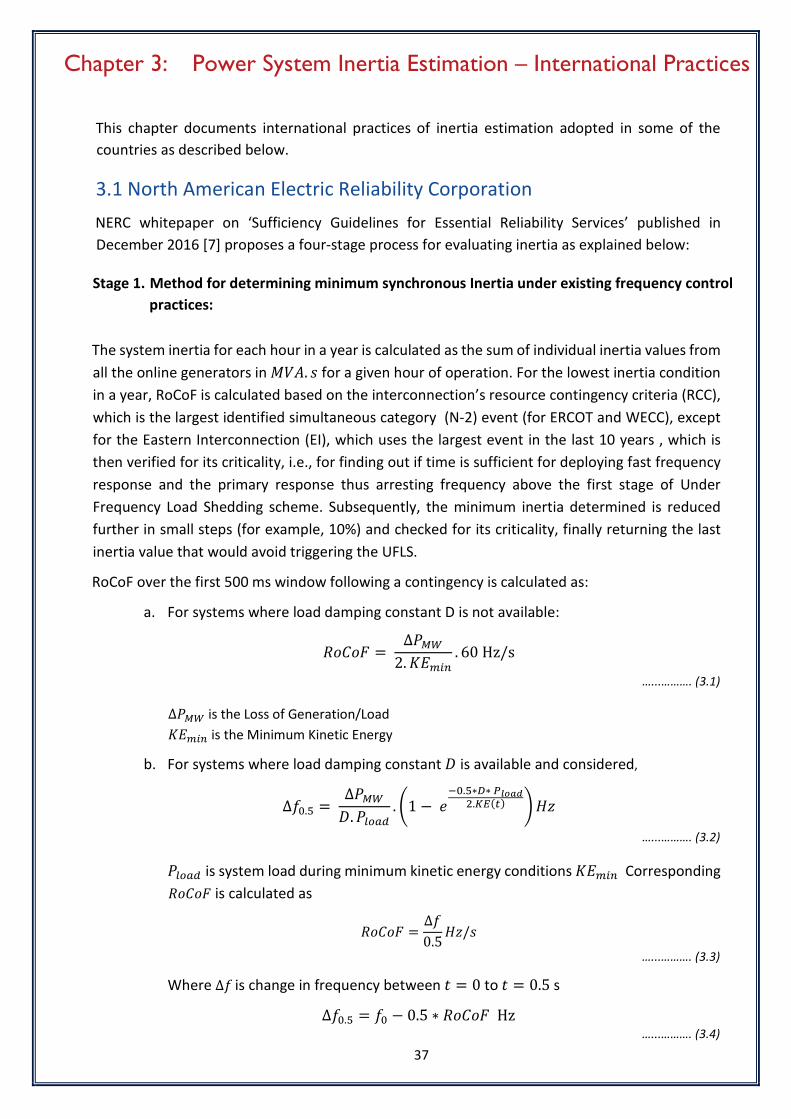
37

Chapter 3: Power System Inertia Estimation – International Practices

This chapter documents international practices of inertia estimation adopted in some of the countries as described below.

3.1 North American Electric Reliability Corporation NERC whitepaper on ‘Sufficiency Guidelines for Essential Reliability Services’ published in December 2016 [7] proposes a four-stage process for evaluating inertia as explained below:

Stage 1. Method for determining minimum synchronous Inertia under existing frequency control practices:

The system inertia for each hour in a year is calculated as the sum of individual inertia values from all the online generators in 𝑀𝑀𝑉𝑉𝑉𝑉. 𝑚𝑚 for a given hour of operation. For the lowest inertia condition in a year, RoCoF is calculated based on the interconnection’s resource contingency criteria (RCC), which is the largest identified simultaneous category (N-2) event (for ERCOT and WECC), except for the Eastern Interconnection (EI), which uses the largest event in the last 10 years , which is then verified for its criticality, i.e., for finding out if time is sufficient for deploying fast frequency response and the primary response thus arresting frequency above the first stage of Under Frequency Load Shedding scheme. Subsequently, the minimum inertia determined is reduced further in small steps (for example, 10%) and checked for its criticality, finally returning the last inertia value that would avoid triggering the UFLS.

RoCoF over the first 500 ms window following a contingency is calculated as:

a. For systems where load damping constant D is not available:

𝑅𝑅𝑅𝑅𝑅𝑅𝑅𝑅𝐹𝐹 = ∆𝑃𝑃𝑀𝑀𝑀𝑀

2.𝐾𝐾𝐸𝐸𝑚𝑚𝑖𝑖𝑛𝑛. 60 Hz/s

…...………. (3.1)

∆𝑃𝑃𝑀𝑀𝑀𝑀 is the Loss of Generation/Load 𝐾𝐾𝐸𝐸𝑚𝑚𝑖𝑖𝑛𝑛 is the Minimum Kinetic Energy

b. For systems where load damping constant 𝐷𝐷 is available and considered,

∆𝑓𝑓0.5 = ∆𝑃𝑃𝑀𝑀𝑀𝑀𝐷𝐷.𝑃𝑃𝑙𝑙𝑙𝑙𝑚𝑚𝑑𝑑

. �1 − 𝑒𝑒−0.5∗𝐷𝐷∗ 𝑃𝑃𝑙𝑙𝑙𝑙𝑙𝑙𝑙𝑙

2.𝐾𝐾𝐾𝐾(𝑧𝑧) �𝐻𝐻𝐻𝐻

…...………. (3.2)

𝑃𝑃𝑙𝑙𝑙𝑙𝑚𝑚𝑑𝑑 is system load during minimum kinetic energy conditions 𝐾𝐾𝐸𝐸𝑚𝑚𝑖𝑖𝑛𝑛 Corresponding 𝑅𝑅𝑅𝑅𝑅𝑅𝑅𝑅𝐹𝐹 is calculated as

𝑅𝑅𝑅𝑅𝑅𝑅𝑅𝑅𝐹𝐹 =∆𝑓𝑓0.5

𝐻𝐻𝐻𝐻/𝑚𝑚 …...………. (3.3)

Where ∆𝑓𝑓 is change in frequency between 𝑡𝑡 = 0 to 𝑡𝑡 = 0.5 s

∆𝑓𝑓0.5 = 𝑓𝑓0 − 0.5 ∗ 𝑅𝑅𝑅𝑅𝑅𝑅𝑅𝑅𝐹𝐹 Hz …...………. (3.4)

38

Stage 2. Verification of actual lowest achievable synchronous inertia under existing frequency control practises

In this approach the minimum synchronous inertia that will be always maintained on-line for a system is calculated from the contribution of the sources, such as

1. Must – Run units 2. Synchronous condensers or generator operating in synchronous mode 3. Industrial generators on-line 4. Nuclear units 5. Generating units providing reserve

The aggregate inertia calculated from the abovementioned sources is compared against the minimum inertia requirement calculated in Stage 1 above, and in case the latter (Stage 1 value) is higher, then based on unit merit the unit commitment would bring additional synchronous generators online one by one till the total system inertia value is close to the theoretical minimum value determined in Stage 1. The results are verified with dynamic simulations using the adjusted unit commitment and simulating a resource contingency criteria (RCC) event.

Stage 3. Trending of synchronous inertia versus minimum inertia value

ERSTF Measures Framework Report iterates that once the minimum inertia based on ROCOF is determined, the continuous monitoring of the synchronous inertia of system against the minimum inertia is emphasised. Forecasting the future system inertia based on the historical trends of system inertia, net load, and planned non-synchronous generation is of importance when system is operating close to minimum inertia level.

A method using historic trends between system inertia and net load, as well as planned non-synchronous generation, to forecast a year ahead minimum system inertia is used. However, during validation of this estimation for the past years, the approach was found to yield results that were overly conservative, hence it was suggested that more accurate prediction of future inertia requires simulation studies by modelling the future generation mix, unit commitment, and dispatch.

Stage 4. Mitigation alternatives at extremely low system inertia

Various strategies to mitigate the impact of low system inertia include:

a. System Operators bring more synchronous generating units on-line only during insufficient inertia conditions

b. Including inertia as a constraint in the unit commitment framework. c. Installing synchronous condensers d. Mitigating under-frequency events by including frequency responsive units in the unit

commitment process e. Synthetic inertial response from Wind

3.2 Australian Energy Market Operator (AEMO) In the report [8], inertia requirements for Australian power system have been discussed. AEMO does not dispatch inertia, however RoCoF constraint is used to limit the rate of change of system frequency in vulnerable regions by controlling power flow over interconnectors. AEMO calculates

39

the inertia requirements for various inertia sub-networks in accordance with the inertia requirements methodology, as specified below:

1. Minimum threshold level of inertia for islanded sub‐network: Here, the inertia threshold is the minimum level of inertia required to operate an inertia sub-network in a satisfactory operating state.

2. Secure operating level of inertia for islanded inertia sub‐network: Here, secure operating level is the minimum level of inertia required to operate an inertia sub-network in a secure operating state.

AEMO has a two–stage approach for determining inertia requirements.

• Stage 1: - Screening of sub-regions that are potentially at risk of inertia shortfall is carried out in this stage. This is based on simple frequency trajectory assessment using SMM.

• Stage 2: - If a sub-region is approaching the minimum threshold level of inertia, a second and more detailed assessment is carried out with the use of a PSCAD/EMTDC model of the sub-region. AEMO did not identify any shortfall of inertia in any region except South Australia.

The Methodology to calculate the inertia requirement is summarised below.

1. Identification of relevant contingencies while islanded: Unit/Station tripping or large industrial load contingency, which would lead to the highest RoCoF (during islanded operation of the inertia area), is considered as a credible contingency.

2. Fast Frequency Control Ancillary Services (FCAS) requirement and Inertia: A power system model of the inertia subnetwork/inertia area is used to assess the frequency trajectory following the contingency events identified at point -1 above. This model is used to establish a relationship between inertia levels and required levels of Fast FCAS response to maintain system frequency within the acceptable/permitted limits.

In low inertia systems, higher volume of FCAS would be required to maintain frequency within the acceptable range, as compared to system with high inertia. For a given demand and contingency size, a typical inverse relationship between Fast FCAS requirement and inertia is shown in Figure 3.1 (a).

Figure 3.1 (a) Fast FCAS requirement & (b) FCAS availability with inertia (AEMO)

Similarly, a linear relationship has been assumed between system inertia and availability of FCAS, as shown in Figure 3.1 (b).

The intersection of the requirement for Fast FCAS and the availability of Fast FCAS characteristics shown above, both as functions of inertia, is therefore used to determine the secure operating level of inertia for an inertia sub-network.

Relationship between Fast FCAS requirement and inertia

Linear relationship assumed between Fast FCAS availability and inertia

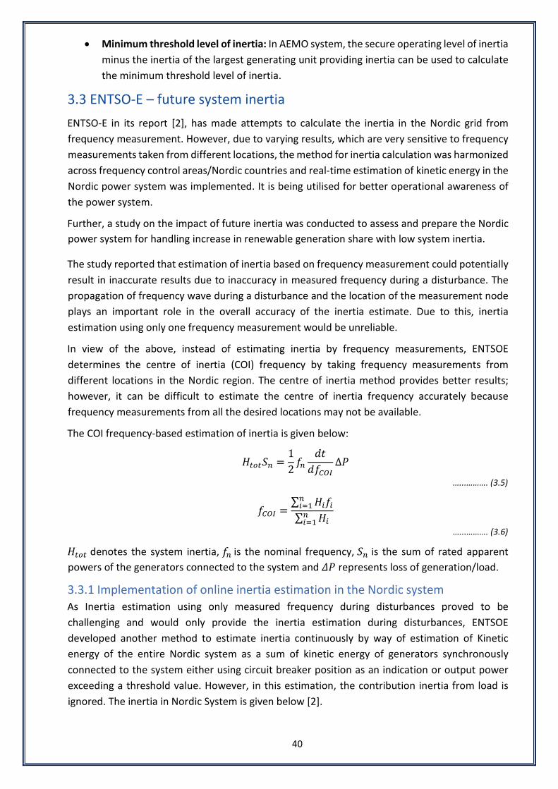
40

• Minimum threshold level of inertia: In AEMO system, the secure operating level of inertia minus the inertia of the largest generating unit providing inertia can be used to calculate the minimum threshold level of inertia.

3.3 ENTSO-E – future system inertia ENTSO-E in its report [2], has made attempts to calculate the inertia in the Nordic grid from frequency measurement. However, due to varying results, which are very sensitive to frequency measurements taken from different locations, the method for inertia calculation was harmonized across frequency control areas/Nordic countries and real-time estimation of kinetic energy in the Nordic power system was implemented. It is being utilised for better operational awareness of the power system.

Further, a study on the impact of future inertia was conducted to assess and prepare the Nordic power system for handling increase in renewable generation share with low system inertia.

The study reported that estimation of inertia based on frequency measurement could potentially result in inaccurate results due to inaccuracy in measured frequency during a disturbance. The propagation of frequency wave during a disturbance and the location of the measurement node plays an important role in the overall accuracy of the inertia estimate. Due to this, inertia estimation using only one frequency measurement would be unreliable.

In view of the above, instead of estimating inertia by frequency measurements, ENTSOE determines the centre of inertia (COI) frequency by taking frequency measurements from different locations in the Nordic region. The centre of inertia method provides better results; however, it can be difficult to estimate the centre of inertia frequency accurately because frequency measurements from all the desired locations may not be available.

The COI frequency-based estimation of inertia is given below:

𝐻𝐻𝑧𝑧𝑙𝑙𝑧𝑧𝑆𝑆𝑛𝑛 =12𝑓𝑓𝑛𝑛

𝑑𝑑𝑡𝑡𝑑𝑑𝑓𝑓𝐶𝐶𝐶𝐶𝐶𝐶

∆𝑃𝑃

…...………. (3.5)

𝑓𝑓𝐶𝐶𝐶𝐶𝐶𝐶 =∑ 𝐻𝐻𝑖𝑖𝑓𝑓𝑖𝑖𝑛𝑛𝑖𝑖=1∑ 𝐻𝐻𝑖𝑖𝑛𝑛𝑖𝑖=1

…...………. (3.6)

𝐻𝐻𝑧𝑧𝑙𝑙𝑧𝑧 denotes the system inertia, 𝑓𝑓𝑛𝑛 is the nominal frequency, 𝑆𝑆𝑛𝑛 is the sum of rated apparent powers of the generators connected to the system and 𝛥𝛥𝑃𝑃 represents loss of generation/load.

3.3.1 Implementation of online inertia estimation in the Nordic system As Inertia estimation using only measured frequency during disturbances proved to be challenging and would only provide the inertia estimation during disturbances, ENTSOE developed another method to estimate inertia continuously by way of estimation of Kinetic energy of the entire Nordic system as a sum of kinetic energy of generators synchronously connected to the system either using circuit breaker position as an indication or output power exceeding a threshold value. However, in this estimation, the contribution inertia from load is ignored. The inertia in Nordic System is given below [2].

41

1. SVENSKA KRAFTNÄT SCADA System: In the Swedish system, kinetic energy is calculated for 421 generators, accounting for maximum available kinetic energy of 166.5 GWs. Moreover, the generator breaker position for at least 125 generators is not visible/accessible to the system operator, and their kinetic energy amounts to 19.22 GWs, which represents 11.54% of the maximum available kinetic energy. Furthermore, inertia constant data of at least 173 small generators is unknown.

2. FINGRID SCADA System: In the Finnish system, circuit breaker positions and power measurements are used to identify the machines synchronised to the system. The online inertia estimation tool in the Finnish system calculates kinetic energy separately for the generating units mentioned below.

a. Combined heat and power b. Industrial back pressure power c. Nuclear power d. Gas turbines e. Peak power plants f. Hydropower g. Condensing power (Condensation Electric Power Plant a thermal steam-turbine

power plant) 3. ENERGINET System: Measurements from all the power plants above 1.5 MW capacity,

available in the Energinet SCADA system are used to calculate the kinetic energy of the Eastern Danish grid (DK2). Circuit breaker positions and power measurements are used to indicate which machines are synchronised to the system. For the generators where circuit breaker positions are not available, generator power measurements are used.

4. STATNETT System: In the Norwegian system, the online inertia estimation is implemented based on the total production level in the system, with an average inertia constant of 3.44 s. This has been estimated based on comparison from the simplified vs the breaker status method.

With the upgrade on the EMS system at Statnett, the Inertia estimation will be done by the more accurate method of using individual generator breaker position and its corresponding inertia.

The comparison of the Breaker status method and total production level has given the following inferences for the Norwegian grid

• Kinetic energy calculated using the total production method fluctuates more due to variation in total production in comparison to the change in the breaker position

• The kinetic energy is too low during the night and too high during daytime in the total production method

3.3.2 Estimation of minimum (maximum) instantaneous frequency The minimum (maximum) instantaneous frequency is calculated using a linear model which is based on

1. Power imbalance caused by a disturbance 2. Power imbalance related to total production

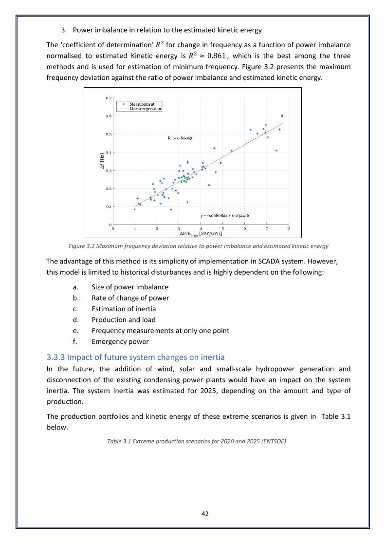
42

3. Power imbalance in relation to the estimated kinetic energy

The ‘coefficient of determination’ 𝑅𝑅2 for change in frequency as a function of power imbalance normalised to estimated Kinetic energy is 𝑅𝑅2 ≈ 0.861 , which is the best among the three methods and is used for estimation of minimum frequency. Figure 3.2 presents the maximum frequency deviation against the ratio of power imbalance and estimated kinetic energy.

Figure 3.2 Maximum frequency deviation relative to power imbalance and estimated kinetic energy

The advantage of this method is its simplicity of implementation in SCADA system. However, this model is limited to historical disturbances and is highly dependent on the following:

a. Size of power imbalance b. Rate of change of power c. Estimation of inertia d. Production and load e. Frequency measurements at only one point f. Emergency power

3.3.3 Impact of future system changes on inertia In the future, the addition of wind, solar and small-scale hydropower generation and disconnection of the existing condensing power plants would have an impact on the system inertia. The system inertia was estimated for 2025, depending on the amount and type of production.

The production portfolios and kinetic energy of these extreme scenarios is given in Table 3.1 below.

Table 3.1 Extreme production scenarios for 2020 and 2025 (ENTSOE)

43

3.4 Ireland All Ireland System has two system operators, Eirgrid in the Republic, and SONI in Northern Ireland. Eirgrid, has rolled out a program, “DS3” (“Delivering a Secure Sustainable Electricity System”), which aims to facilitate high penetration of renewable energy in the system.

The program aims to find a secure way to operate the Irish power system today and in the future. A focus of the program is related to the delivery of new ancillary services, and synchronous inertial response is one of them. As the first step in this direction, Ireland has installed an inertia monitoring platform in the control room of the TSO to warn operators if the inertia available from synchronized generators drops below a pre-determined level.

EIRGRID, in its report [9], has conducted a techno-economic study to determine the volume of synchronous and/or synthetic inertia required in order to maintain the RoCoF at 0.5 Hz/s whilst also achieving levels of 75% System Non-Synchronous Penetration (SNSP). Technical studies were performed based on the generation dispatches produced from the power market modelling tool Plexos and Powertech’s DSA Tools PSAT is used to create power-flows, these power-flows are fed into the frequency stability simulations (TSAT package) (refer Figure 3.3).

44

Figure 3.3 Overview of the Automated Dynamic Study tool process

To maintain the rate of change of frequency (RoCoF) within ±0.5 Hz/s (calculated over 500 ms) for an N-1 event which are the tripping of Large Single Infeed/Outfeed has been considered in the study. Simulations are considered as secure if the RoCoF criterion is satisfied for the worst-case contingency. The base case scenario is executed, and if the RoCoF requirement is not met, supplementary inertia is added to the system until the number of secure cases in the full year dispatch is in the 99th percentile. The inertia level which ensures 99 percentile dispatch cases are secure is deemed as the inertia requirement for the system.

RoCoF is calculated using the following equation

𝑅𝑅𝑅𝑅𝑅𝑅𝑅𝑅𝐹𝐹 = System frequency × Active powerlost2(Inertiasystem−Inertialost)

…...………. (3.7)

The following is concluded in the study.

3.5 National Grid UK System The National Grid in the UK has been using a basic inertia estimation approach by monitoring the online transmission-connected generators while accounting for an estimate of inertia from the embedded generation and demand for quite some time. However, with the increasing share of renewable generation, the National Grid has employed two new approaches to obtain a more accurate estimate [10]. The first approach is the deployment of Effective Inertia measurement and forecasting toll from GE Digital. The measured value of effective inertia is claimed to capture inertia from rotating synchronous generation and the inertia-like effects of non-synchronous generation, such as wind and solar PV, and passive responses from the domestic and industrial demand. Inertia is estimated on a regional basis, using measurements of grid frequency and power flows.

45

The second approach is carried out in partnership with a company ‘Reactive Technologies’, which uses a signal-injection-based method to measure inertia. Battery storage or ultra-capacitors are used to inject a pulse through the power grid, whose response is measured and processed by the Extensible Measurement Unit (XMU) and a cloud computing platform.

3.6 Inferences for estimation of inertia of Indian power system Based on the literature survey and review of international best practices, the following is gathered for implementation in Indian power system:

1. A methodology for determining minimum synchronous inertia may be considered for Indian system.

2. The online inertia estimation using circuit breaker position and individual inertia constant of units could be implemented to determine the inertia of generators. However, lack of sufficient data with adequate accuracy (parameters and measurements) is likely to affect the accuracy of the estimation.

3. Inertial contribution from the load side, which can be potentially as high as 20% depending on the load type, needs to be considered in the overall inertia estimation in Indian power system

4. Offline estimation of inertia based on the Centre of Inertia (COI) could be computed from the available frequency measurements of naturally occurring events

5. The inertia estimation practices being used by various system operators have their own limitations, which are now claimed to be addressed in several advanced approaches reported in the literature. Such advanced approaches can be explored in Indian grid for better quality inertia estimation.

6. Considering that Indian power system will experience a significant penetration of renewable energy generation in the coming years, estimation of potential inertial contribution from such power electronic interfaced sources may be considered in the system inertia estimation framework.

46

Chapter 4: Inertia of Generating Units in India

4.1 Sources of Inertia in Power system

4.1.1 Conventional Generators The synchronous generators can be broadly classified as thermal, nuclear, hydro, and Renewable Energy sources (RES). The thermal generators are further classified on the basis of fuel being utilised, e.g., coal, lignite, gas, and diesel. The hydro plants less than 25 MW of capacity are generally considered as small hydro plants and they fall under RES. RES mainly consists of Solar plants, Wind plants, Biomass Power, Urban & Industrial Waste Power. With a total installed capacity of around 392 GW (as of November 2021), various generation sources in terms of their installed capacity in different regions of India are summarised in Table 4.1.

Table 4.1 Region wise installed capacity in India [Source: National Power Portal]

Region Thermal

Nuclear Renewable

Total Total Total

NR 62769 1620 44110 108499 WR 85923 1840 39787 127550 SR 55470 3320 57767 116557 ER 27966 0 6473 34440

NER 2526 0 2368 4894 Islands 40 0 38 78

All India 234694 6780 150544 392017 (All values in MW)

The generator technology wise breakup of all India installed generation capacity indicates that the major proportion of generation is from synchronously connected generation. RES based generation sources, as can be observed from Figure 4.1, comprise a significant proportion of total generation.

Figure 4.1 Installed generation capacity in India

The source wise breakup of RE based sources (as of November 2021) is given in Table 4.2 below.

Coal52%

Lignite2%

Gas6%

Diesel~0%

Nuclear2%

Hydro 12%

RES*(MNRE)26%

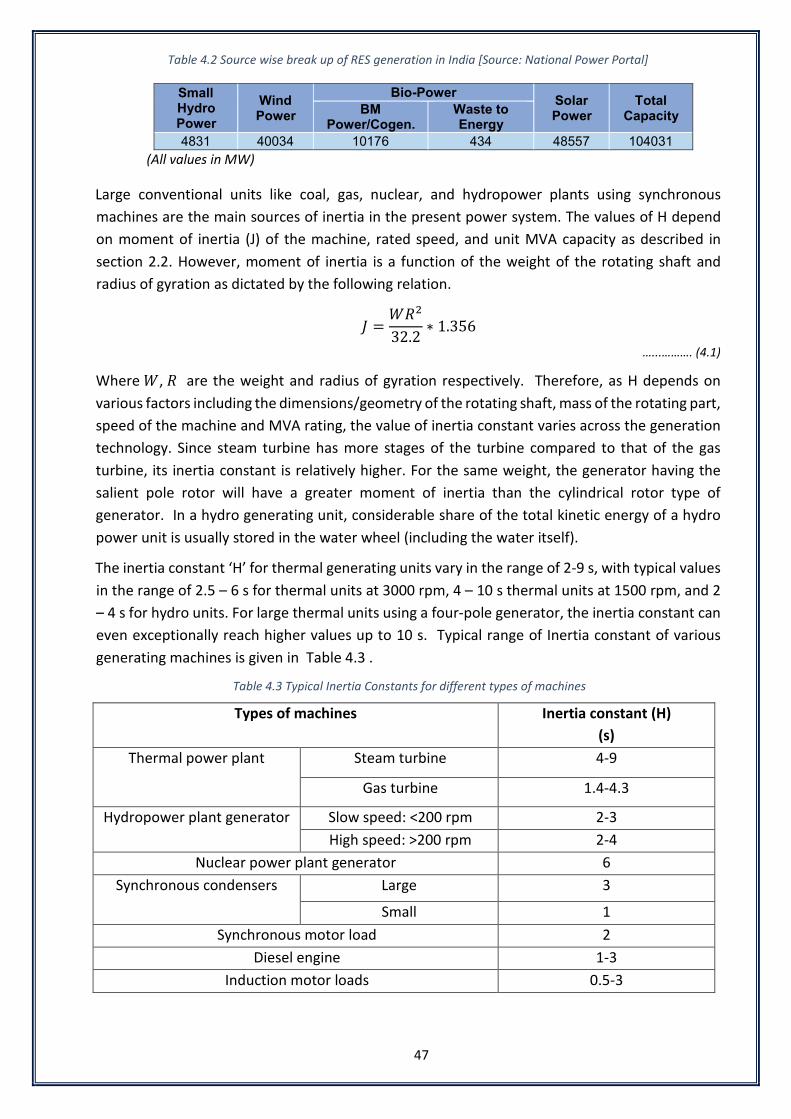
47

Table 4.2 Source wise break up of RES generation in India [Source: National Power Portal]

Small Hydro Power

Wind Power

Bio-Power Solar Power

Total Capacity BM

Power/Cogen. Waste to Energy

4831 40034 10176 434 48557 104031 (All values in MW)

Large conventional units like coal, gas, nuclear, and hydropower plants using synchronous machines are the main sources of inertia in the present power system. The values of H depend on moment of inertia (J) of the machine, rated speed, and unit MVA capacity as described in section 2.2. However, moment of inertia is a function of the weight of the rotating shaft and radius of gyration as dictated by the following relation.

𝐽𝐽 =𝑊𝑊𝑅𝑅2

32.2∗ 1.356

…...………. (4.1)

Where 𝑊𝑊, 𝑅𝑅 are the weight and radius of gyration respectively. Therefore, as H depends on various factors including the dimensions/geometry of the rotating shaft, mass of the rotating part, speed of the machine and MVA rating, the value of inertia constant varies across the generation technology. Since steam turbine has more stages of the turbine compared to that of the gas turbine, its inertia constant is relatively higher. For the same weight, the generator having the salient pole rotor will have a greater moment of inertia than the cylindrical rotor type of generator. In a hydro generating unit, considerable share of the total kinetic energy of a hydro power unit is usually stored in the water wheel (including the water itself).

The inertia constant ‘H’ for thermal generating units vary in the range of 2-9 s, with typical values in the range of 2.5 – 6 s for thermal units at 3000 rpm, 4 – 10 s thermal units at 1500 rpm, and 2 – 4 s for hydro units. For large thermal units using a four-pole generator, the inertia constant can even exceptionally reach higher values up to 10 s. Typical range of Inertia constant of various generating machines is given in Table 4.3 .

Table 4.3 Typical Inertia Constants for different types of machines

Types of machines Inertia constant (H) (s)

Thermal power plant Steam turbine 4-9

Gas turbine 1.4-4.3

Hydropower plant generator Slow speed: <200 rpm 2-3 High speed: >200 rpm 2-4

Nuclear power plant generator 6 Synchronous condensers Large 3

Small 1 Synchronous motor load 2

Diesel engine 1-3 Induction motor loads 0.5-3

48

In this report, the inertia constants of generating units in India with ratings higher than 50 MW in Northern, Western, Southern & Eastern regions, and higher than 25 MW in North-Eastern region, have been analysed. The source of inertia constants of the generating units used in this report is by the generator nameplate data, estimated value for the units whose parameters were not available and, and in some cases, results of onsite testing of primary frequency response has been used.

The effort has been made to identify any correlation of inertia constant with the rating of the generating unit. No clear consistency could be arrived at for the inertia constant of generating plants with rating or fuel type. The inertia constant of each category of conventional generation plants in Indian grid is discussed below.

4.1.2 Inertia constant of thermal (coal-fired) generating units in India In Indian grid, the maximum share of kinetic energy reserves provided by thermal units due to its largest proportion in the overall generation mix. The relevant data for a total of 667 number of thermal units with their aggregate kinetic energy of 894 GW-s was available and therefore included in this analysis. The median of the Inertia constant of all thermal units in the Indian power system is 3.3 s, while the maximum unit inertia among thermal units was observed to be 6.22 s for a generating unit of 960 MVA capacity. The range of inertia constant of units lying between 25 to 75 percentiles is in the range of 2.73 to 4.05 s. Unit-wise inertia constant along with their rated capacity in MVA is plotted in Figure 4.2. The inertia constant of generators was also analysed based on make, manufacturer, and vintage. It was found that similar rating thermal generators are having a variation in their inertia constants, which can be primarily attributed to their design and technology advancement that generally improves with time. Consequently, in some cases, it has been observed that the inertia constants for the new generators are comparatively lower than those of old ones.

49

Figure 4.2 Inertia constant of Thermal Generators in India

4.1.3 Inertia constant of hydro generating units in India Hydro units contribute the second highest primary frequency response following the corresponding contribution from thermal units.

The information on a total of 358 number of hydro units was available and therefore included in the analysis. While total kinetic energy available from all the considered hydro units is 146.8 GW-s, average kinetic energy available per unit is 410 MW-s. The median of the Inertia constant of all hydro units in the Indian power system is 3.66 MW-s/MVA. The maximum unit inertia in hydro units is 6 s for a 278 MVA hydro generator. The range of inertia constant of units lying between 25 to 75 percentiles is in the range of 3 to 3.94 s. Unit-wise inertia constant plotted against their rated capacity in MVA is provided in Figure 4.3. Large modern hydro generators tend to have smaller inertia constant compared to the old ones of similar capacity, and may face issues related to the turbine governing system stability. This decreasing inertia constant trend can be attributed to the turbine water behaviour, which due to its inertia can lead to water hammers in pressure pipes when control devices are operated, which is generally characterized by the hydraulic acceleration time constants. In islanded operation where the turbine governor determines the system frequency, the water hammer affects the speed governing system leading to instability driven hunting or frequency swings. For interconnected operations with a large system, the frequency is essentially held constant by the main grid, and the water hammer in this case affects the power fed to the system and stability problem only arises when the power is controlled in a closed-loop.

0

1

2

3

4

5

6

7

0 200 400 600 800 1000 1200

INER

TIA

CON

STAN

T(H

) IN

MW

-SEC

/MVA

UNIT CAPACITY IN MVA

Thermal UnitsFrom Gen Data Sheet Assumed

50

Figure 4.3 Inertia constant of Hydro Generators in India

4.1.4 Inertia constant of gas turbine generating units in India Data of 128 number of gas units was available and included in the analysis. The total kinetic energy available from these gas units is 55.7 GW-sec. The average kinetic energy available per unit is 435 MW-s. The median of the Inertia constant of all gas units in the Indian power system is 2.73 s. The minimum inertia of gas plants is the lowest at 0.91s among all types of generators. The mean of gas units is comparatively lower than that of thermal units, which can be primarily attributed to lower shaft mass and low capacity gas turbines. The maximum unit inertia among gas turbine units was 5.2 s for a unit capacity of 400 MVA. The range of inertia constant of units lying between 25 to 75 percentiles is in the range of 1.4 to 3 s. Unit-wise inertia constant along with their rated capacity in MVA is provided in Figure 4.4.

0

1

2

3

4

5

6

7

0 50 100 150 200 250 300

INER

TIA

CON

STAN

T(H

) IN

MW

-SEC

/MVA


Hydro UnitsFrom Gen Data Sheet Assumed

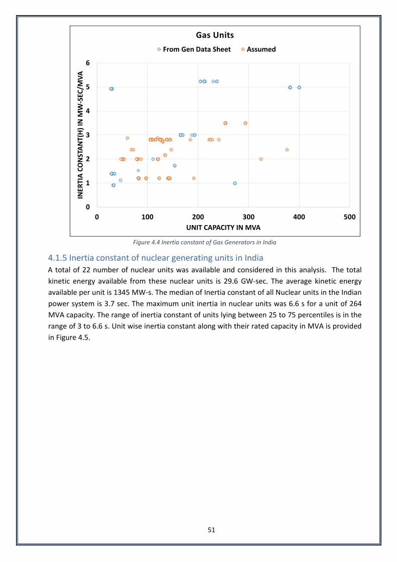
51

Figure 4.4 Inertia constant of Gas Generators in India

4.1.5 Inertia constant of nuclear generating units in India A total of 22 number of nuclear units was available and considered in this analysis. The total kinetic energy available from these nuclear units is 29.6 GW-sec. The average kinetic energy available per unit is 1345 MW-s. The median of Inertia constant of all Nuclear units in the Indian power system is 3.7 sec. The maximum unit inertia in nuclear units was 6.6 s for a unit of 264 MVA capacity. The range of inertia constant of units lying between 25 to 75 percentiles is in the range of 3 to 6.6 s. Unit wise inertia constant along with their rated capacity in MVA is provided in Figure 4.5.

0

1

2

3

4

5

6

0 100 200 300 400 500

INER

TIA

CON

STAN

T(H

) IN

MW

-SEC

/MVA


Gas UnitsFrom Gen Data Sheet Assumed

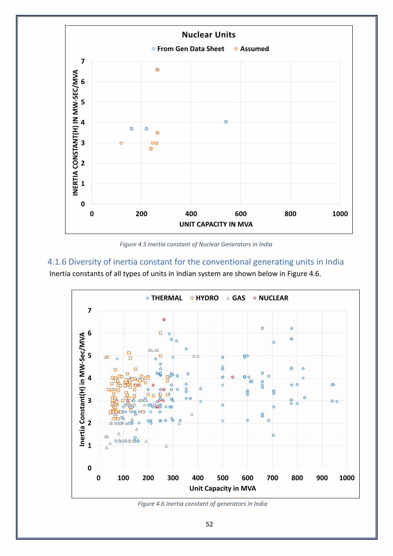
52

Figure 4.5 Inertia constant of Nuclear Generators in India

4.1.6 Diversity of inertia constant for the conventional generating units in India Inertia constants of all types of units in Indian system are shown below in Figure 4.6.

Figure 4.6 Inertia constant of generators in India

0

1

2

3

4

5

6

7

0 200 400 600 800 1000

INER

TIA

CON

STAN

T(H

) IN

MW

-SEC

/MVA


Nuclear UnitsFrom Gen Data Sheet Assumed

0

1

2

3

4

5

6

7

0 100 200 300 400 500 600 700 800 900 1000

Iner

tia C

onst

ant(

H) i

n M

W-S

ec/M

VA

Unit Capacity in MVA

THERMAL HYDRO GAS NUCLEAR

53

In Indian power system, based on the median value of inertia constant of each category of generator, it has been observed that thermal generation has highest inertia contribution followed by hydro, gas and nuclear.

The range of Inertia constant of all types of generating units can be observed in the box and whiskers plot provided in Figure 4.7. The broad range of thermal units’ inertia constant shows the diversity of thermal unit sizes in Indian system. Inertia Constant of Generators Region wise is given in annexure I.

Figure 4.7 Box and Whiskers plot of Inertia constant of generators in India

The amount of inertia available from a generating unit is independent of the power generated by it.

Synchronous condensers are spinning synchronous machine connected to high voltage and provide dynamic voltage control by varying the excitation current. As they are synchronously connected to the system, they will also contribute to the total inertia. However, as they do not generate any active power, no prime mover is driving the synchronous machine. Consequently, the stored kinetic energy in synchronous condenser is rather low compared to the generating station of the same unit capacity. A general thumb rule is that synchronous condensers have around 1/3rd of inertia of the corresponding generating unit of the same MVA capacity. The description of synchronous condensers is given in detail at Annexe-2 of this report.

4.1.7 Inertia contribution from load Inertia contribution from the load side is considered to be the second highest with generation side inertia contribution being the main source of overall system inertia. Inertia contribution from the load side is projected to be as high as 20% of the total system inertia. However, the actual inertia contribution from the demand depends on various factors, such as, load composition, frequency and voltage sensitivity of the load, and load side regulations. Since it is practically difficult to determine the exact load composition, coupled with uncertainty and variability of

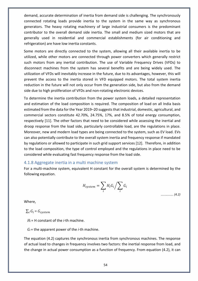
54

demand, accurate determination of inertia from demand side is challenging. The synchronously connected rotating loads provide inertia to the system in the same way as synchronous generators. The heavy rotating machinery of large industrial consumers is the predominant contributor to the overall demand side inertia. The small and medium sized motors that are generally used in residential and commercial establishments (for air conditioning and refrigeration) are have low inertia constants.

Some motors are directly connected to the system, allowing all their available inertia to be utilized, while other motors are connected through power converters which generally restrict such motors from any inertial contribution. The use of Variable Frequency Drives (VFDs) to disconnect machines from the system has several benefits and are being widely used. The utilization of VFDs will inevitably increase in the future, due to its advantages, however, this will prevent the access to the inertia stored in VFD equipped motors. The total system inertia reduction in the future will not only occur from the generation side, but also from the demand side due to high proliferation of VFDs and non-rotating electronic devices.

To determine the inertia contribution from the power system loads, a detailed representation and estimation of the load composition is required. The composition of load on all India basis estimated from the data for the Year 2019–20 suggests that industrial, domestic, agricultural, and commercial sectors constitute 42.70%, 24.75%, 17%, and 8.5% of total energy consumption, respectively [11]. The other factors that need to be considered while assessing the inertial and droop response from the load side, particularly controllable load, are the regulations in place. Moreover, new and modern load types are being connected to the system, such as EV load. EVs can also potentially contribute to the overall system inertia and frequency response if mandated by regulations or allowed to participate in such grid support services [12]. Therefore, in addition to the load composition, the type of control employed and the regulations in place need to be considered while evaluating fast frequency response from the load side.

4.1.8 Aggregate inertia in a multi machine system For a multi-machine system, equivalent H constant for the overall system is determined by the following equation.

𝐻𝐻𝑚𝑚𝑠𝑠𝑚𝑚𝑧𝑧𝑒𝑒𝑚𝑚 = �𝐻𝐻𝑖𝑖𝐺𝐺𝑖𝑖𝑖𝑖

�𝐺𝐺𝑖𝑖𝑖𝑖

�

…...………. (4.2)

Where,

∑ 𝐺𝐺𝑖𝑖𝑖𝑖 = 𝐺𝐺𝑚𝑚𝑠𝑠𝑚𝑚𝑧𝑧𝑒𝑒𝑚𝑚

Hi = H constant of the i-th machine.

Gi = the apparent power of the i-th machine.

The equation (4.2) captures the synchronous inertia from synchronous machines. The response of actual load to changes in frequency involves two factors: the inertial response from load, and the change in actual power consumption as a function of frequency. From equation (4.2), it can

55

be concluded that with the increase of the number of rotating machines the value of inertia constant will increase, and hence the overall inertia of the power system will be higher.

In the survey carried out for Indian power system, inertia constant of more than 1175 generating units with combined rating of around 316 GVA has been analysed. The units with rating more than 50 MVA were considered for NR, WR, SR, ER and units with rating more than 25 MVA were considered for NER.

The summary based on inertia constant values of generating units for all the five regional grids and at All India level is shown in Table 4.4.

Table 4.4 Kinetic energy based on survey on sources of inertia

Region

Thermal Gas Hydro Nuclear Total

Total Capacity

(GVA)

Kinetic Energy (GW- sec)

Total Capacity

(GVA)


Total Capacity

(GVA)


Total Capacity

(GVA)


Total Capacity

(GVA)


NR 52.5 197.0 6.0 14.4 16.6 64.3 1.8 5.8 76.9 281.5 WR 90.2 301.0 9.7 37.3 6.1 21.3 1.8 7.1 107.8 366.7 SR 57.4 207.0 0.8 1.6 10.2 36.0 3.8 16.7 72.2 261.3 ER 48.5 184.0 - - 7.0 23.0 - - 55.5 207.0 NER 0.8 5.0 1.5 2.4 1.3 2.2 - - 3.6 9.6 All India 249.4 894.0 18.0 55.7 41.2 146.8 7.4 29.6 316.0 1126.1

Based on the values given in Table 4.4 , it is observed that total kinetic energy available from the sources of inertia is around 1126 GW-sec. The distribution of sources of inertia indicate that Western region has largest amount of resources for kinetic energy. It may not be technically correct to arrive at an inertia value based on contribution of all such units as it is understood that all the considered generating units are unlikely to be simultaneously grid connected. However, a rough estimate based on all sources of inertia included in survey, the approximate maximum value of inertia constant has been found as 3.56 sec at 316 GVA base. However, for any estimate of system wide inertia, contribution of the demand side needs to be considered.

4.2 Inertia contribution from Renewable Energy sources The increasing share of renewable energy resources with power electronic converter interface has a significant impact on system inertia at higher RE penetration level. Following a large disturbance, the overall system inertia from all the synchronous sources helps in maintaining a stable operation by restricting the RoCoF. However, unlike synchronous machines, the presence of the power electronic interface in renewable energy sources decouples the generation side from the grid frequency, and hence, such sources unlike synchronous generation, do not provide an inherent inertial response following a system disturbance.

Hence, with increased penetration of IBRs and the displacement of conventional sources, the effective inertia of the system is expected to reduce, thereby affecting the dynamic system performance. Even though the IBRs do not provide an inherent inertial response, additional virtual inertia controls can be implemented to provide an emulated inertial response from such

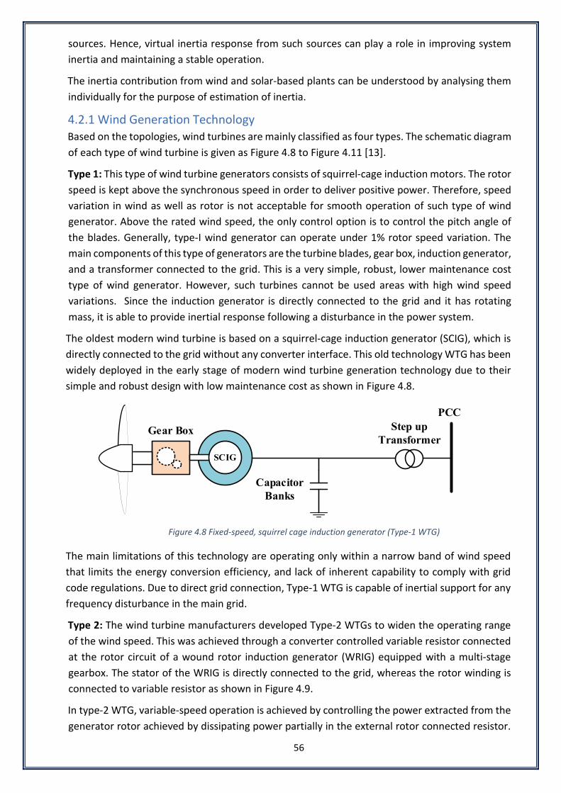
56

sources. Hence, virtual inertia response from such sources can play a role in improving system inertia and maintaining a stable operation.

The inertia contribution from wind and solar-based plants can be understood by analysing them individually for the purpose of estimation of inertia.

4.2.1 Wind Generation Technology Based on the topologies, wind turbines are mainly classified as four types. The schematic diagram of each type of wind turbine is given as Figure 4.8 to Figure 4.11 [13].

Type 1: This type of wind turbine generators consists of squirrel-cage induction motors. The rotor speed is kept above the synchronous speed in order to deliver positive power. Therefore, speed variation in wind as well as rotor is not acceptable for smooth operation of such type of wind generator. Above the rated wind speed, the only control option is to control the pitch angle of the blades. Generally, type-I wind generator can operate under 1% rotor speed variation. The main components of this type of generators are the turbine blades, gear box, induction generator, and a transformer connected to the grid. This is a very simple, robust, lower maintenance cost type of wind generator. However, such turbines cannot be used areas with high wind speed variations. Since the induction generator is directly connected to the grid and it has rotating mass, it is able to provide inertial response following a disturbance in the power system.

The oldest modern wind turbine is based on a squirrel-cage induction generator (SCIG), which is directly connected to the grid without any converter interface. This old technology WTG has been widely deployed in the early stage of modern wind turbine generation technology due to their simple and robust design with low maintenance cost as shown in Figure 4.8.

Step upTransformer

Gear Box

Capacitor Banks

SCIG

PCC

Figure 4.8 Fixed‐speed, squirrel cage induction generator (Type‐1 WTG)

The main limitations of this technology are operating only within a narrow band of wind speed that limits the energy conversion efficiency, and lack of inherent capability to comply with grid code regulations. Due to direct grid connection, Type-1 WTG is capable of inertial support for any frequency disturbance in the main grid.

Type 2: The wind turbine manufacturers developed Type-2 WTGs to widen the operating range of the wind speed. This was achieved through a converter controlled variable resistor connected at the rotor circuit of a wound rotor induction generator (WRIG) equipped with a multi-stage gearbox. The stator of the WRIG is directly connected to the grid, whereas the rotor winding is connected to variable resistor as shown in Figure 4.9.

In type-2 WTG, variable-speed operation is achieved by controlling the power extracted from the generator rotor achieved by dissipating power partially in the external rotor connected resistor.

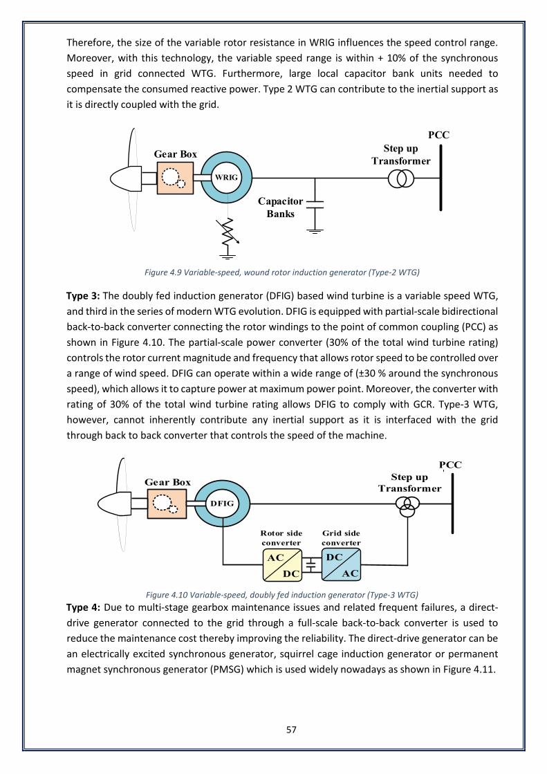
57

Therefore, the size of the variable rotor resistance in WRIG influences the speed control range. Moreover, with this technology, the variable speed range is within + 10% of the synchronous speed in grid connected WTG. Furthermore, large local capacitor bank units needed to compensate the consumed reactive power. Type 2 WTG can contribute to the inertial support as it is directly coupled with the grid.

Step upTransformerGear Box

Capacitor Banks

PCC

WRIG

Figure 4.9 Variable‐speed, wound rotor induction generator (Type‐2 WTG)

Type 3: The doubly fed induction generator (DFIG) based wind turbine is a variable speed WTG, and third in the series of modern WTG evolution. DFIG is equipped with partial-scale bidirectional back-to-back converter connecting the rotor windings to the point of common coupling (PCC) as shown in Figure 4.10. The partial-scale power converter (30% of the total wind turbine rating) controls the rotor current magnitude and frequency that allows rotor speed to be controlled over a range of wind speed. DFIG can operate within a wide range of (±30 % around the synchronous speed), which allows it to capture power at maximum power point. Moreover, the converter with rating of 30% of the total wind turbine rating allows DFIG to comply with GCR. Type-3 WTG, however, cannot inherently contribute any inertial support as it is interfaced with the grid through back to back converter that controls the speed of the machine.

Step upTransformer

Grid side converter

Rotor side converter

Gear Box

PCC

AC

DC

DC

AC

DFIG

Figure 4.10 Variable‐speed, doubly fed induction generator (Type‐3 WTG)

Type 4: Due to multi-stage gearbox maintenance issues and related frequent failures, a direct-drive generator connected to the grid through a full-scale back-to-back converter is used to reduce the maintenance cost thereby improving the reliability. The direct-drive generator can be an electrically excited synchronous generator, squirrel cage induction generator or permanent magnet synchronous generator (PMSG) which is used widely nowadays as shown in Figure 4.11.

58

Step upTransformer

Grid side converter

Machine side converter

PMSGAC

DC

DC

AC

PCC

Figure 4.11 Variable‐speed, permanent magnet synchronous generator (Type‐4 WTG)

The main advantage of the full-scale converter-based wind turbine is the wide operating range of wind speed variations and the decoupled control of active and reactive power injection at PCC. However, compared to DFIG, Type-4 WTG is of cost due to full rated back-to-back converter, yet it is generally preferred for offshore sites owing to lower maintenance cost due to the absence gearbox, which is a maintenance-intensive component. The full-scale back-to-back converter-based wind turbine is decoupled from the grid, thus, the WTG cannot inherently detect the grid disturbances, and hence cannot provide any grid support service including inertial support inherently.

For commercially available fixed-speed wind turbine generators with more than 1 MW rating, the inertia constant ‘H’ varies between 3–5 s. Therefore, it is evident that fixed speed wind turbines are capable of providing inertial support to the system. Indian power system while having large number of old wind turbine generators, is also experiencing high integration of DFIG based wind turbine generators.

4.2.2 Solar Photovoltaic Generation The parameters that define the characteristics of a PV panel are the rated/ maximum power (P_mp), maximum power point voltage (V_mp), maximum power point current (I_mp), open circuit voltage (V_oc), and short circuit current (I_sc). The operating point of the panel of a PV system can be altered by controlling the PV terminal voltage. The PV panels are connected with the grid through power electronic converter interfaces. There are four main topologies of PV power plants, depending on how the PV panels are connected to the inverters units: central, string, multistring, and module integrated topologies. PV power plants can be broadly classified in rooftop and utility scale power plants. In solar photovoltaic plants, there are no rotating parts involved and no inherent inertia is available from them. However, solar PV based plants have capability to increase their output over full range in a very short span of time. The fast response obtained from the PV plant can provide inertial response, if the PV inverter is operating under deloaded condition.

4.2.3 Energy Storage System Energy storage systems are employed in the power system for improved efficiency, reliability, demand side management, and as a source of fast and primary frequency response. The rapid development in power electronics and ESS technologies resulted in increased use of such technologies for various applications in power systems. The different forms of storage energy include chemical batteries, supercapacitors, flywheels, and pumped hydro storage systems. Lead-acid batteries, sodium-sulfur batteries, vanadium redox batteries, and li-ion batteries are

59

examples of ESS that are currently in use for FFR applications with relatively lower costs. At the same time, superconducting magnetic energy storage based ESS with a fast discharge rate and short response time has been expensive to implement in grid-scale applications. The energy storage systems can broadly be classified into four different categories, (i) wind farm connected ESS, (ii) wind turbine connected ESS, (iii) PV power plant connected ESS, and (iv) distributed energy storage systems (DESS). The RE sources with an ESS can provide considerably higher FFR response, e.g., an ESS-WTG hybrid system can deliver 45% more inertial power as compared with a wind turbine alone. In addition to the stationary grid scale storage, EVs offer an option of mobile storage that through aggregation can be potentially used as grid scale storage.

4.3 Synthetic Inertia from non-synchronous generation sources Currently, the power generation mix in India is dominated by conventional power plants that are based on synchronous generators. In future scenarios, Indian power system will experience a high share of variable Renewable Energy Sources (RES), such as Wind Turbine Generators (WTG) and Photovoltaic Systems (PV) connected to the electrical grid through power electronic converters. Hence, the RE-driven displacement of conventional generators is likely to diminish overall system inertia in the future, such as in 2022, 2030 and beyond.

Since adequate system inertia is critical for power system stability - more precisely grid frequency stability, a sufficient amount of inertia is necessary for secure and stable grid operation. Inertia limits the rate of change of frequency (ROCOF) in the first few seconds from the onset of a sudden power imbalance. Hence, mechanisms to control grid frequency are facilitated with sufficient time to adapt power output and re-establish power system balance. Therefore, there is a need to address the issue of diminishing inertia in large scale RE integrated power systems.

One of the potential solutions to address diminishing inertia is to employ so-called “synthetic inertia” or “virtual inertia”. Synthetic inertia can be defined as inertial support from non-synchronous generation, controllable load, or energy storage devices that emulate the inertial response of a synchronous generator by employing a suitable control technique and a power electronic interface. Depending on the control topology employed, virtual inertia sources can deliver an electrical power output that is proportional to the rate of change of frequency (RoCoF) and/or frequency deviation during a frequency event.

The virtual inertia control temporarily provides fast power in response to a credible frequency event. For instance, inertia response from the wind turbines can release energy from the rotational mass in the turbine to provide this temporary power increase or employ short term overloading to provide additional power from wind, if operating at rated power. The inertial support (in the form of additional power production during a drop-in frequency) of the wind turbine is limited not only by the low speed limits but also by the setting of various controllers.

4.3.1 Synthetic inertia from Wind generators As discussed earlier in this chapter, there are four different types of wind turbine generators (WTG) that are used in wind power conversion. Type 1 (SCIG) and Type 2 (WRIG) WTGs form the predominant share of the WTGs installed in the past. However, both the type1 and type-2 WTGs are obsolete technology and are no more being manufactured. Therefore, almost all the new

60

WTGs being installed in the system currently are Type 3 (DFIG wind turbine) and Type 4 (full power converter wind turbine) WTGs.

In Type 4 WTG, the rated electrical output of the generator available over a wide range of frequency can be converted to grid frequency by using back to back converter. This means that the wind turbine generator can be operated over a wide range of speeds. In addition, the grid side converter can independently control real and reactive power exchange with grid. It is to be noted that the rotor of the wind turbine is not magnetically coupled to the grid frequency and is controlled to maximize active power production.

Presently, the Indian Electricity Grid Code does not mandate a provision for inertial response capability from Solar PV and wind power plants. Inertial/frequency response features for wind and solar PV plants is commercially available technology and mandated in some countries. Therefore, considering Indian grid with high RE penetration in the future, incorporation of inertial support features in utility scale IBRs in IEGC regulation may be considered in due consultation with the key stakeholders.

4.3.2 Synthetic inertia from Battery Energy Storage Systems Synthetic inertial control is implemented relatively easily using standalone battery energy storage systems. Moreover, a battery energy storage system can be implemented together with other RE source to provide a superior inertial response characteristic and to enable optimal use of the available renewable resource.

Ample studies on the implementation of synthetic inertia with different battery energy storage types and control topologies are available in the literature. The control topologies can range from a very complex implementation of the synchronous machine dynamical equations to deliver inertial response, to a very simple droop or RoCoF based response. Moreover, the type of energy storage can also influence the speed of inertial response that can be delivered.

Even though virtual inertia response with battery storage units is quite attractive, the cost of the system can play a decisive role in the number of storage units used to improve system stability. Moreover, the cost of the storage technology deployed can also dictate the maximum available power and duration power response (available energy, i.e., the capacity).

With the rise of electric vehicles (EV), mobile battery storage systems can also potentially be utilized for provision of synthetic inertia. Although restricted by the relatively small size of individual EV batteries, aggregation of EV fleets can make these storage systems comparable or even larger than utility scale storage. However, proper coordination among the different entities, well developed regulations and advanced electricity markets would be required for EVs to participate in provision of synthetic inertia [12]

4.3.3 Synthetic inertia from PV Systems In a solar photovoltaic plant, there are no rotating parts involved, and hence stored no kinetic energy or inertia is inherent. However, there are two different ways in which virtual inertia response can be implemented in a photovoltaic power plant. The first method involves operating the plant at a sub-optimal output and utilizing the remaining available power margin to provide an inertial response when required. Such operation is known as derated operation of solar PV, and the plant is operated below its maximum power operating pot. The second method involves

61

the use of a battery energy storage system in conjunction with the PV plant, which is typically operated at its maximum power output level. During a frequency event, the required inertial response is derived from the additional battery unit.

62

Chapter 5: Measurement based System Inertia Estimation

In Chapter 3 and Chapter 4, inertia and its various contributing sources have been discussed in detail including the synthetic inertia from non-synchronous sources. Utilizing the mathematical and physical relationship derived in the previous chapters, this chapter focuses on the estimation of grid Inertia through post-mortem analysis of the recorded frequency response to naturally occurring contingency and swing equation in the offline mode. This chapter highlights the estimated inertia of the Indian Grid for several numbers of frequency events and various other associated parameters that can be estimated based on the measured data. It also tries to find out the inertia variation and its dependence on various factors.

5.1 Literature Survey on evaluation of inertia estimation methods from measurement data A detailed literature survey for measurement-based inertia estimation approaches has been carried out, and some of the methods analysed are summarised in Table 5.1 below.

Table 5.1 Measurement based methods for inertia calculation Source Key points

Application of Phasor Measurement Units to Estimate Power System Inertial Frequency Response [14]

1. Assumption: A delay of up to 1 second from the onset of generation loss is assumed before primary response in the form of generator governor action and additional static services responds to the deviation in frequency.

2. Type of Frequency Events Considered: Event where all the units in a power plant tripped simultaneously rather than staggered tripping.

3. Detrended fluctuation analysis (DFA) Method: To detect the start of the event and to identify event suitability for H estimation.

4. Not Considered: Location of PMU devices in Network however that impact has not been considered in this paper (Whether to Use suitable measurement or weighed average or COI need to be worked out in future work)

Estimation of power system inertia constant and capacity of spinning-reserve support generators using measured frequency transients

[4]

1. Base to be used for Inertia Constant Representation in Swing Equation: System Load Base

2. Data Used: Transients of the frequency measured event such as a generator load rejection

3. ROCOF Calculation: A polynomial approximation with respect to time is applied to the waveform of the transients to restrain the influence of the oscillatory component in estimating the inertia constant.

4. Frequency Measurement to be used: Average system frequency is used. Moreover, intermachine

63

Source Key points oscillations due to synchronizing power and transmission performance are not considered, while equivalent system inertia, generator and load are assumed.

5. Identification of Start Time: To identify the time of the onset of the event, the instant at which RoCoF value breaches a threshold (0.04 Hz/sec) is taken the start time.

Estimation of Inertia Constant of Iran Power Grid Using the Largest Simulation Model and PMU Data [15]

Data Used: Weighted average of ROCOF from PMU frequency for first 400 ms were for inertia calculation using Swing Equation.

Monitoring of Frequency Disturbances in the European Continental Power System [16]

1. The system inertia appears to be concentrated around 8-10 sec.

2. Use minimum value of ROCOF estimated for inertia estimation

ENTSO-E Report on Future system inertia [2]

1. Provides a survey of work earlier done for calculation of system inertia using frequency measurements from events.

2. The initial behaviour of frequency following a frequency disturbance varies over different locations compared with the centre of inertia frequency. The superimposed oscillatory component frequency and amplitude is considered to be dependent on the operational scenario and fault location.

3. Centre of Inertia frequency can be observed visually where oscillatory component will be negligible and can be used as CoI for calculating Inertia.

4. Using arbitrary frequency measurements from inertia estimation will fail to provide the correct inertia of the system.

5. CoI for different scenario and different events varies and is not represented by same node all the time. It is essential to find the neutral node for each event. However, due to measurements non-observability, it will not always be possible to find a neutral location.

6. The centre of inertia model provides inaccurate results when a trip causes changes in bus voltages which in turn lead to changes in the system load. This is because the model assumes that changes in the system load are negligible which, according to the simulations, is not a valid assumption. In reality, it is very difficult to estimate the change in the system load. It may be

64

Source Key points possible to use voltage measurements to assess the reliability of the results.

7. While the centre of inertia method offers the best results, it is challenging to estimate centre of inertia frequency accurately.

Power System Inertia Estimation by Approaching Load Power Change After a Disturbance [17]

1. An offline estimation method is proposed in this paper, which aims to estimate the power change of the loads due to voltage dependency after a disturbance.

2. At present most of the existing studies have focused on estimating inertia using frequency measurements after a disturbance.

3. An aggregated load model is considered which aims to approach the behaviour of the average system load. This aggregated load is monitored and approximated by the data available at the generator buses. The load model selected for the method is exponential, static, represents constant current characteristics.

4. It has been shown that the method performs better when it is applied shortly after the disturbance when the impact from load frequency dependency and governor response is particularly low.

5. The proposed method is also powerful when applied later point when applied at various times between 100 ms to 500 ms after the disturbance. The behaviour of the method was gradually deteriorating with time, but the mean error remained under 10%.

However, the estimation errors increased when the load modelling of the system was different than the one considered by the method.

Online Estimation of Power System Inertia Using Dynamic Regressor Extension and Mixing [18]

1. An algorithm is proposed which allows estimating the inertia constant and the aggregated mechanical power setpoint of a large-scale power system. The algorithm is derived using a first-order nonlinear aggregated power system model in combination with the recently proposed dynamic regressor and mixing (DREM) procedure.

2. The performance of the estimator is demonstrated on a 1013-machine ENTSO-E test system. The considered scenarios for this purpose investigated in the paper consist of 25 generator outages and a rescheduling event.

65

Source Key points 3. In addition to the inertia constant, the aggregated mechanical power setpoint of the PFC generators is also estimated.

The response of the aggregated system based on the estimated inertia matches the simulated one with an error of only a few mHz.

Simultaneous Estimation of the Time of Disturbance and Inertia in Power Systems [19]

1. An online algorithm for simultaneous estimation of the time of disturbance and the inertia after a disturbance is proposed.

2. The proposed algorithm is designed to operate online using active power and frequency measurements from a wide area monitoring system.

3. The swing equation, with damping neglected, to model the frequency dynamics of the system immediately after a disturbance is used for the estimation.

4. This algorithm uses a set of sliding data windows to continuously calculate candidate inertia estimates. These candidate estimates will converge to the true inertia during a disturbance.

Simulations, laboratory tests, and real transmission system measurements have been used to demonstrate the validity of the proposed method.

Inertia Estimation of the GB Power System Using Synchrophasors Measurements [3]

1. An approach to estimate the total inertia of the GB power system using synchronized phasor measurement units.

2. Estimation work is carried out by dividing the network into groups or regions of generation based around the constraint boundaries of the GB network. The inertia is first estimated at a regional level before it is combined to provide a total estimate for the whole network.

3. The proposed method first detects a suitable event for analysis using detrended fluctuation analysis (DFA), and then filter the measured transients in order to obtain a reliable estimate of inertia.

4. This estimate is then compared with the known contribution to inertia from generation, to provide an estimate for the currently unknown contribution from other residual sources such as namely synchronously connected demand and embedded generation.

The proposed method is demonstrated on the full dynamic model of the GB transmission system, and also

66

Source Key points using a number of instantaneous transmissions in-feed loss events in the GB transmission network.

Measuring effective area inertia to determine fast-acting frequency response requirements [20]

1. A method to estimate the effective inertia of an area/region of a power system is proposed to help system operators understand the overall frequency stability of the area.

2. The effective inertia is characterized by the relation between the power transfer in/out of the area, and the observed RoCoF of the area.

3. PMU measurements of total generation loads and net power transfer across the area boundary is used to detect a suitable event and estimate the required area inertia.

The outcome of the study points to the understanding and importance of inertial effects on an area basis, owing to differences in frequency, ROCOF and phase angle across the system. Moreover, the proposed effective inertia takes into account for the other responses to grid frequency changes, including load-voltage dependency.

Based on the literature survey, the challenges in inertia calculation can be summarized as follows:

1. Lack of time-synchronized data from the various nodes distributed across the system and associated data quality issue.

2. Selection of appropriate Frequency node to be used in the swing equation for inertia estimation.

3. Issue of Oscillatory nature of system frequency during disturbances resulting from relative motion of generators and Locational Impact of measured frequencydata.

4. Selection of Node representing the Centre of Inertia if the time synchronized data from various nodes in the grid is available. Finding a centre of Inertia during a dynamic event is challenging.

5. Choice of utilising Centre of Inertia frequency for system RoCoF calculation does not yield satisfactory results due to different RoCoF observed at different locations in the system during a frequency event

6. Accuracy of calculated RoCoF from frequency data which is influenced by frequency data quality, time interval used, or the Curve fitting methods used to calculate RoCoF.

7. Accounting for inertia contribution from non-synchronous resources

5.2 Approach for measurement-based inertia estimation in Indian power system Based on literature survey and international practices, a methodology for measurement-based inertia estimation for Indian system has been developed, which is discussed in this section. The

67

proposed method is based on frequency measurements from the synchrophasor data using the swing equation describing COI. The procedure developed utilizes the following key features:

1. Assumption: It is assumed that just after the event solely the System Inertia determines the initial ROCOF. While the contribution of inertia at the onset of the disturbance from the demand side is neglected for the current framework, it will be accounted in the developed approach in the future.

2. System Base: System Base considered for Inertia Estimation for Indian Grid is All India Generation (MW) during the event.

3. Type of Frequency Events Considered: Event where the entire power plat is tripped, rather than staggered tripping of units with the plant.

4. Input Data: All Indian Frequency Plots from PMU data and All India Generation Prior to Event from SCADA are obtained.

5. PMU data: System-Wide inertia is considered by using the time synchronised frequency measurements of various locations from the grid.

6. Event Start Identification: Based on Frequency plot, the time at which adjacent frequency data difference is larger than the threshold value due to frequency fall.

7. Curve Fit: A fifth or sixth order polynomial is applied to the frequency data to minimize the influence of the frequency signal oscillation.

8. ROCOF Calculation: Based on 5 or 6th order polynomial fit for average frequency or COI frequency, the initial maximum ROCOF is determined.

The steps followed for inertia estimation based on the above procedure are described below:

Figure 5.1 Frequency response plots from PMUs (a) raw data (b) smoothened data Step 1: All Indian Frequency Plots from PMU measurement and All India generation prior to the event from SCADA are obtained (Figure 5.1(a)) Step 2: PMU data is filtered for a smooth frequency plot (Figure 5.1(b)).

68

Figure 5.2 (a) Average frequency response (b) Selected window for curve fitting

Step 3: Average Frequency of these PMU data calculated and plotted (Figure 5.2 (a)), and pre-disturbance frequency is determined.

Step 4: Frequency window starting from the onset of the event is used in curve fitting approach (Figure 5.2 (b)).

Figure 5.3 Frequency response and its polynomial fit

Step 5: Using the Scatter plot and curve fitting method for 5th order polynomial to find its equation and determining initial RoCoF from the curve fit equation (Figure 5.3).

The frequency response obtained in Figure 5.3 is considered to be representative of frequency response observed at the centre of inertia node. Various attributes viz. initial RoCoF, net frequency drop and time to reach nadir point are illustrated in Figure 5.4.

69

Figure 5.4 Approximate frequency response and other parameters of centre of inertia

Table 5.2 summarises the inertia estimation related data for Indian system from the identified contingency.

Table 5.2 Details of the Frequency event considered for Inertia estimation Date and Time 21-Jan-2019 15:57

Initial Frequency (Hz) 49.885

All India Generation (From NLDC SCADA)1 (MW) 144482

Actual Generation Loss (SCADA) (MW) 780

Calculated ROCOF from Avg Frequency (Hz/s) 0.0167

Estimated inertia (sec) 8.06

Nadir Frequency (Hz) 49.804

Time to Reach Nadir Frequency (sec) 10.6

Frequency Drop (Hz) 0.0810

Power Number =∆𝑃𝑃/∆𝑓𝑓 (MW/Hz) 9626.65 Two aspects which need to be considered in detail while analysing the inertia calculated from the adopted approach are as following:

1. Captive power generation is not under monitoring in India at National/Regional Control centre which ranges from 10-15 % of total generation.

2. Utilisation of monitored MW in place of MVA base in calculation of inertia.

1 It is to be noted that NLDC SCADA while having observability of most the conventional generation sources, some embedded generation, particularly of low capacity is not captured in the SCADA data. The estimation approach will be further improved by accounting for such generation in the future

70

5.3 Challenges in measurement based inertia estimation Based on the summary of the literature survey, several key issues have been highlighted in the utilization of frequency measurements for inertia estimation. These challenges have been discussed below along with the suggested solution.

1. Time synchronization issues: The grid frequency measurements after any frequency event are available in the form data recorders placed in the power system. However, to accurately calculate the inertia, the frequency measurements should be having very higher sampling rate which is not possible with the conventional SCADA system. This issue can be tackled by collecting the data from the Data acquisition system (DAS) from generators. However, in a large system like Indian grid, the number of generators will be large and the data from these generators may not be time synchronized thus making it difficult to use the data for inertia calculation.

This issue is illustrated in Figure 5.5 where frequency data from different nodes is plotted.

The issue of non-time synchronized data and high sample rate data can be potentially addressed with the help of Synchrophasor measurement data. The Synchrophasor data are currently being reported to SLDC/RLDC/NLDC at 25 samples per second and are time synchronized. In addition, the data is being centrally collected at SLDC/RLDC/NLDC level thus making it easily available.

2. Data Quality Issue: Data quality issues can impact the calculation of RoCoF. RoCoF computed from SCADA data may be inaccurate due to low sampling rate. These aspects can be observed from Figure 5.6. To resolve this issue, Synchrophasor data can be used as they are highly accurate data with low noise level due to existence of inherent filters at the device level. However, in Synchrophasor data also, those data have to be used which have higher accuracy and low noises as shown in Figure 5.7 .Thus, Synchrophasor data has come out as a good data source for the estimation of RoCoF using the swing equation.

Figure 5.5 Typical time synchronization issues in high resolution frequency data

71

Figure 5.6 Frequency from PMU and SCADA for the

same event Figure 5.7 Frequency data from two PMUs for

the same event

4. Calculation of RoCoF: The Rate of change of frequency (RoCoF) parameter can be obtained by

two methods from the Synchrophasor data. It includes RoCoF directly reported by the Synchrophasor unit, and the other is calculated RoCoF from the reported frequency measurement. It has been observed from the literature survey that the RoCoF reported from PMUs is generally not used. In literature, it has been reported that rather than utilizing the RoCoF at its reporting rate from PMU (25 -50 Samples per seconds), researchers and industry had utilized the filtered RoCoF so that initial noises can be avoided. For calculation of inertia from the swing equation, the RoCoF required is at 𝑡𝑡 = 0, therefore various studies utilize the frequency data along with curve fitting algorithm [2,4].

5. Selection of Event for Inertia estimation: While estimating inertia in offline mode there is also a need to identify the ∆𝑃𝑃 which will be causing the frequency event in the system. In power system, frequency is changing dynamically) prior to the frequency event which is due to load generation imbalance in the system. Under such condition, it is essential to see whether the frequency rise is steady due to normal generation or load change in system or due to any past frequency response event. In Indian Power system as per the existing Grid Code Regulation, a ripple factor of ± 0.03 Hz has been kept to avoid generator governor operation for any steady rise/fall in frequency in the system. So, event where there is no precursor frequency event then for those events, the ∆𝑃𝑃 for the event is known. However, if cases where one event has occurred followed by another event then in such cases the governor has already started providing response and in such case the ∆𝑃𝑃 will be the governor response being gradually provided due to previous event and the load/gen loss in the next event. In such condition calculation of exact ΔP is difficult and utilizing such event of inertia calculation will not yield correct result in absence of required information. A simplified dynamic equation representing the relation between frequency dynamics with power unbalance is as below [18]:

𝜔𝜔𝐶𝐶𝐶𝐶𝐶𝐶̇ =𝜔𝜔02

2𝐻𝐻𝑧𝑧𝑙𝑙𝑧𝑧𝑆𝑆𝐵𝐵�𝑃𝑃𝑚𝑚,𝑧𝑧𝑙𝑙𝑧𝑧 + 𝑃𝑃𝑃𝑃𝑃𝑃𝐶𝐶,𝑧𝑧𝑙𝑙𝑧𝑧 + 𝑃𝑃𝑒𝑒,𝑧𝑧𝑙𝑙𝑧𝑧

𝜔𝜔𝐶𝐶𝐶𝐶𝐶𝐶�

…...………. (5.1)

Where,

𝑃𝑃𝑃𝑃𝑃𝑃𝐶𝐶.𝑧𝑧𝑙𝑙𝑧𝑧= Primary frequency response total output 𝑃𝑃𝑚𝑚.𝑧𝑧𝑙𝑙𝑧𝑧= Total mechanical input

72

𝑃𝑃𝑒𝑒.𝑧𝑧𝑙𝑙𝑧𝑧=Total electrical output 𝐻𝐻𝑧𝑧𝑙𝑙𝑧𝑧 = Total inertia constant of the power system 𝜔𝜔0= Nominal network frequency Johannes Schiffer et al have addressed by approximating the primary response present in the system using a simplified aggregated model of the turbine-governor dynamics [18].

However, to avoid any complexity and sources of inaccuracy due to primary response, event having cascaded tripping of generation/load or frequency events which have occurred in close proximity of time are not utilized.

For the Indian power system inertia estimation using frequency measurements, frequency data recorded by PMUs is utilized from across the grid to find the Centre of Inertia (CoI) and then using curve fitting approach, the initial RoCoF can be calculated from this node frequency measurement.

Based on the above-developed procedure, frequency data for 29 Frequency events since 2014 onwards were utilized to calculate the grid inertia which is discussed in detail in Chapter 6.

73

Chapter 6: Inertia Estimation in Indian Power System

6.1 Inertia Estimation Results from Frequency Measurements Naturally occurring generation loss events provide an opportunity for the estimation of power system inertia. A total of 29 such events listed below in Table 6.1, and spanned over 2014 -2021 period were selected for estimation of inertia.

Table 6.1 Details of the Frequency events considered for Inertia estimation

Date Time Initial Frequency

(Hz) All India Generation

(MW) Gen Loss

(MW) 17-Jan-2014 01:26 50.140 102681 624

20-May-2014 19:57 49.997 130339 1850 19-Sep-2014 12:56 50.003 119587 749 13-Nov-2014 12:46 50.017 119962 847 08-Feb-2015 18:31 50.098 115862 608 30-Apr-2016 15:01 50.063 140819 1025 01-May-2016 12:24 50.036 127854 1092 05-Jun-2017 22:20 49.998 152218 1220 27-Nov-2017 08:34 49.995 147082 622 03-Jun-2018 16:26 50.093 140274 654 10-Jul-2018 08:14 50.033 152520 1025

07-Aug-2018 14:07 49.881 156768 880 30-Oct-2018 19:22 49.943 163047 2247 16-Jan-2019 12:27 49.965 155310 1400 21-Jan-2019 15:57 49.885 145355 780 24-Jan-2019 17:14 49.931 142942 1000 12-Apr-2019 23:55 50.032 164570 1865 16-Apr-2019 23:37 50.021 149115 1118 22-May-2019 20:57 49.966 173000 1050 05-Jul-2019 03:56 49.894 153438 1500

21-Aug-2019 00:02 49.923 156774 1364 16-Sep-2019 12:56 49.976 145337 1050 01-Nov-2019 11:16 50.029 129899 1644 29-Dec-2019 07:53 50.004 154230 780 18-Jan-2020 12:36 49.968 154116 1091 26-Dec-2020 10:18 50.045 177572 1011 19-Feb-2021 15:26 49.984 158314 1300 10-Mar-2021 19:35 50.008 175101 1507 24-Mar-2021 12:16 50.021 177845 1586 08-Apr-2021 00:33 49.993 162029 1045 11-Jun-2021 16:02 50.088 164295 1500

Synchrophasor data was obtained for the events listed above in Table 6.1, and estimation of inertia was determined as discussed below.

74

6.1.1 All India Generation vs. Grid Inertia The Indian power system inertia has varied between 5 to 9 Seconds between Jan 2014-June 2021 as shown in Figure 6.1. The mean value of inertia is 6.5 seconds. It can be further observed that even though the inertia is on the higher side, the net inertia is reducing even with higher generation in the system.

Figure 6.1 All India Demand Vs Inertia for 2014‐2021

6.1.2 Grid Inertia variation on year and hour scale The Indian power system inertia calculated for the events when plotted w.r.t. year scale, it was observed ( Figure 6.2) that over the years it has a reducing trend. Further, during the day scale if these events are plotted irrespective of years (Refer Figure 6.3) then, it is observed that inertia is low during the peak hours and higher in the off-peak hours. The reason attributable for this can be higher penetration of solar, lower availability of kinetic energy from the generators, a lower amount of rotating load (Agricultural load is generally connected in off-peak hours) etc.

2

3

4

5

6

7

8

9

10

11

100 110 120 130 140 150 160 170 180

Iner

tia (S

ec)

All India Demand (GW)

All India Demand (GW) Vs Indian Grid Inertia (Sec)

Bubble size is Proportional to Kinetic Energy (GW-s)

75

Figure 6.2 Grid Inertia on Year Scale

Figure 6.3 Grid Inertia vs Time of Day

6.1.3 Inertia Vs. RE Penetration Due to RE driven displacement of conventional synchronous generation, the system experiences lower system inertia. The impact of higher Renewable penetration on the system inertia in Indian grid is reflected in Figure 6.4. It is to be noted that for the period over which the plot in Figure 6.4 is shown, the overall generation (including conventional generation) installed capacity of All India grid increased, however, the general trend shows that the system is becoming lighter with the increase in RE penetration assuming no contribution from renewable generation. A significant number of type 1 wind turbine generators are installed in India that also contribute to the system inertia to some extent as they are directly coupled with the grid. However, variable speed wind turbine generators (Type-3 and Type-4) are not required to provide inertia in India.

76

Figure 6.4 RE Penetration Vs Grid Inertia

6.1.4 Generation loss vs. Total Frequency Drop The generation loss relationship with frequency drop is also important for the system planners and operators as it helps in deciding the various defense mechanism for frequency stability in the power system. Figure 6.5 shows that a linear trend exists between the amount of generation loss and frequency drop observed in the Indian power system. This trend also depends also on the amount of load damping and governor. With the increase in frequency insensitive load, such as electronic or VFD based load, the slope of the overall frequency dip in Figure 6.5 will increase, while as case of improvement in governor response, the corresponding slope is likely to decrease.

Figure 6.5 Generation Loss vs. Frequency Drop

The ratio of total generation loss with the quantum of frequency fall till nadir point provides good information for system operators. This number may be referred to as power number for the Indian grid. Higher the number, more is the load damping and governor response from the system. It helps in immediate assessment of the generation loss during an event by evaluating the frequency drop, which can also help in the approximation of generation loss by automation and thus

77

providing system operator with an alarm in case of any frequency related events. Figure 6.6 shows the power number plotted for the events (involving load/generation loss over 1000 MW) over between 2014 and 2021. It can be observed that it has an increasing trend over the time indicating that the governor response is improving over the years. The improvement in governor repose in the Indian power system can be visualized in the form of improvement in frequency response characteristics (FRC) for the various frequency related event as discussed in the report. However, it is important to note that the frequency response improvement in Indian grid is a combined effect of various efforts in Indian power sector that have taken place over the past several years, such as, DSM and ancillary services.

Figure 6.6 Power number during different grid events in India

6.3 Impact on Power System Inertia during Covid-19 Pandemic The Indian power system has experienced a significant variation in demand and supply due to the nationwide lockdown imposed from 25th March 2020 due to the Covid-19 pandemic. The lockdown had resulted in a drastic reduction in industrial and commercial demand, resulting in a reduction of around 30-40% in the total All India demand. Due to the lower overall demand and to maintain the load-generation portfolio, a large number of synchronous generators were taken off-line. The loss of online synchronous generations has had a significant impact on the overall inertia of the Indian power system and the associated ROCOF. Furthermore, the gradual phase-wise relaxations of the lockdown resulted in a gradual recovery of the load by the end of May 2020.

In order to summarise the impact of Covid-19 on Inertia of the Indian Power System, total four Generation Loss events have been considered as provided in Table 6.2. It can be observed that as expected the overall system inertia of the system reduced to 7.22 s during the lockdown period, while corresponding value for power number reduced to around 7500 MW/Hz

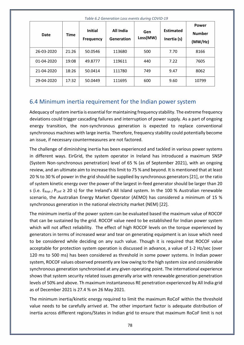
78

Table 6.2 Generation Loss events during COVID‐19

Date Time Initial

Frequency

All India

Generation Gen

Loss(MW) Estimated

Inertia (s)

Power

Number

(MW/Hz)

26-03-2020 21:26 50.0546 113680 500 7.70 8166

01-04-2020 19:08 49.8777 119611 440 7.22 7605

21-04-2020 18:26 50.0414 111780 749 9.47 8062

29-04-2020 17:32 50.0449 111695 600 9.60 10799

6.4 Minimum inertia requirement for the Indian power system Adequacy of system inertia is essential for maintaining frequency stability. The extreme frequency deviations could trigger cascading failures and interruption of power supply. As a part of ongoing energy transition, the non-synchronous generation is expected to replace conventional synchronous machines with large inertia. Therefore, frequency stability could potentially become an issue, if necessary countermeasures are not factored.

The challenge of diminishing inertia has been experienced and tackled in various power systems in different ways. EirGrid, the system operator in Ireland has introduced a maximum SNSP (System Non-synchronous penetration) level of 65 % (as of September 2021), with an ongoing review, and an ultimate aim to increase this limit to 75 % and beyond. It is mentioned that at least 20 % to 30 % of power in the grid should be supplied by synchronous generators [21], or the ratio of system kinetic energy over the power of the largest in-feed generator should be larger than 20 s (i.e. Eksys / PLinf ≥ 20 s) for the Ireland’s All Island system. In the 100 % Australian renewable scenario, the Australian Energy Market Operator (AEMO) has considered a minimum of 15 % synchronous generation in the national electricity market (NEM) [22].

The minimum inertia of the power system can be evaluated based the maximum value of ROCOF that can be sustained by the grid. ROCOF value need to be established for Indian power system which will not affect reliability. The effect of high ROCOF levels on the torque experienced by generators in terms of increased wear and tear on generating equipment is an issue which need to be considered while deciding on any such value. Though it is required that ROCOF value acceptable for protection system operation is discussed in advance, a value of 1-2 Hz/sec (over 120 ms to 500 ms) has been considered as threshold in some power systems. In Indian power system, ROCOF values observed presently are low owing to the high system size and considerable synchronous generation synchronised at any given operating point. The international experience shows that system security related issues generally arise with renewable generation penetration levels of 50% and above. Th maximum instantaneous RE penetration experienced by All India grid as of December 2021 is 27.4 % on 26 May 2021.

The minimum inertia/kinetic energy required to limit the maximum RoCoF within the threshold value needs to be carefully arrived at. The other important factor is adequate distribution of inertia across different regions/States in Indian grid to ensure that maximum RoCoF limit is not

79

breached anywhere in the system irrespective of the size, location and loading state of the Indian grid. An attempt to find the minimum system inertia/kinetic energy requirement in Indian grid through a scientific approach is being explored to determine the inertia threshold values.

Achieving net zero carbon emissions by 2070 is envisaged. In such a scenario, generation technologies such hydro (including pumped hydro), nuclear, biomass, green hydrogen fired gas turbines, and thermal generation with carbon capture & sequestration need to be kept on the radar in view of inertia requirements.

6.5 Summary The outcome of the measurement-based inertia estimation and its analysis reported for Indian grid while considering a set of naturally occurring events is summarised as follows:

1. The Indian power system inertia varied between 5 to 9 seconds between Jan 2014-June 2021 with a mean value of 6.5 s.

2. Indian power system inertia shows a reducing trend which can be primarily attributed to increase in renewable penetration in the system.

3. It has been observed that in some cases, power system inertia is lower in the peak hours while higher in off peak hours. This could be attributed to a higher amount of solar PV generation during peak hours followed by non-availability of agricultural loads.

4. The increase in frequency response with decreasing inertia and rotating load during frequency events indicates the combined governor response has improved in the system.

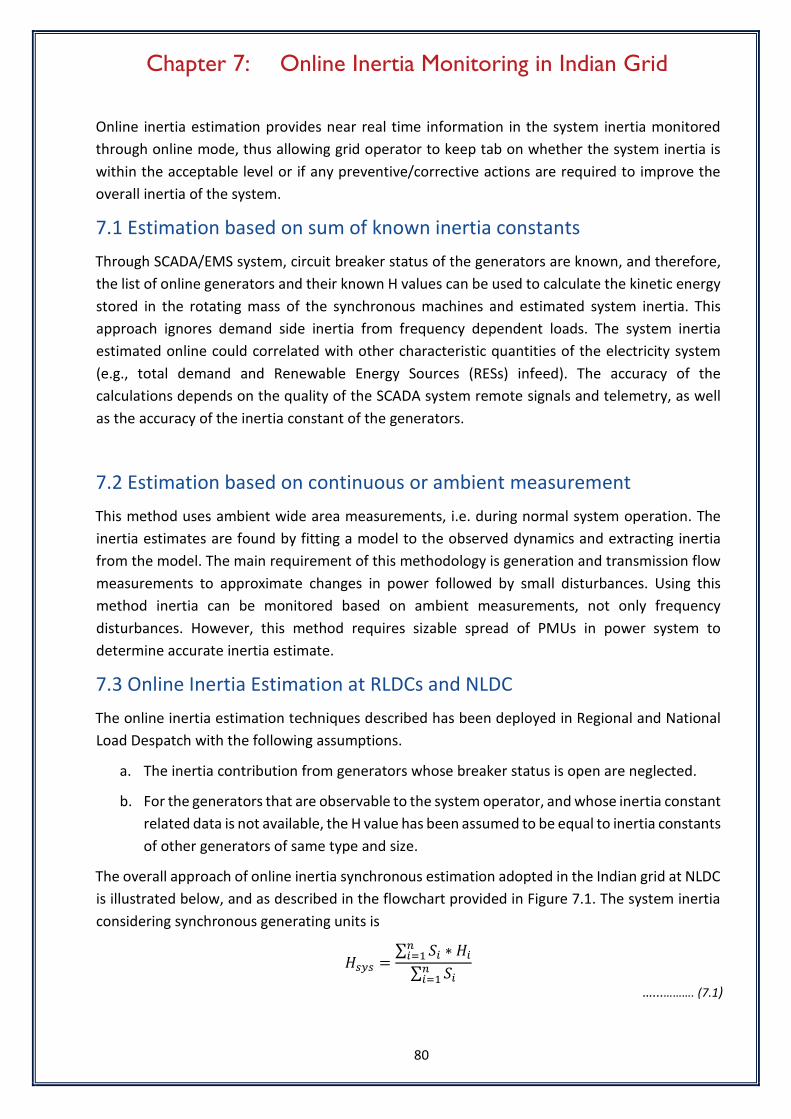
80

Chapter 7: Online Inertia Monitoring in Indian Grid

Online inertia estimation provides near real time information in the system inertia monitored through online mode, thus allowing grid operator to keep tab on whether the system inertia is within the acceptable level or if any preventive/corrective actions are required to improve the overall inertia of the system.

7.1 Estimation based on sum of known inertia constants Through SCADA/EMS system, circuit breaker status of the generators are known, and therefore, the list of online generators and their known H values can be used to calculate the kinetic energy stored in the rotating mass of the synchronous machines and estimated system inertia. This approach ignores demand side inertia from frequency dependent loads. The system inertia estimated online could correlated with other characteristic quantities of the electricity system (e.g., total demand and Renewable Energy Sources (RESs) infeed). The accuracy of the calculations depends on the quality of the SCADA system remote signals and telemetry, as well as the accuracy of the inertia constant of the generators.

7.2 Estimation based on continuous or ambient measurement This method uses ambient wide area measurements, i.e. during normal system operation. The inertia estimates are found by fitting a model to the observed dynamics and extracting inertia from the model. The main requirement of this methodology is generation and transmission flow measurements to approximate changes in power followed by small disturbances. Using this method inertia can be monitored based on ambient measurements, not only frequency disturbances. However, this method requires sizable spread of PMUs in power system to determine accurate inertia estimate.

7.3 Online Inertia Estimation at RLDCs and NLDC The online inertia estimation techniques described has been deployed in Regional and National Load Despatch with the following assumptions.

a. The inertia contribution from generators whose breaker status is open are neglected.

b. For the generators that are observable to the system operator, and whose inertia constant related data is not available, the H value has been assumed to be equal to inertia constants of other generators of same type and size.

The overall approach of online inertia synchronous estimation adopted in the Indian grid at NLDC is illustrated below, and as described in the flowchart provided in Figure 7.1. The system inertia considering synchronous generating units is

𝐻𝐻𝑚𝑚𝑠𝑠𝑚𝑚 =∑ 𝑆𝑆𝑖𝑖 ∗ 𝐻𝐻𝑖𝑖𝑛𝑛𝑖𝑖=1∑ 𝑆𝑆𝑖𝑖𝑛𝑛𝑖𝑖=1

…...………. (7.1)

81

The system inertia calculated at NLDC using sum of known inertia constants can be validated using system inertia computed based on frequency disturbances. Based on validation results the online inertia estimation based on known inertia constants can further be tuned.

Figure 7.1 Flow chart for online inertia estimation

Screenshots of online inertia monitoring tools of different control centres are shown below, Figure 7.2 to Figure 7.7. Apart from kinetic energy, percentage renewable penetration, number of units online, total capacity of the units online and renewable generation are also indicated.

82

Figure 7.2 Online inertia monitoring in NRLDC EMS

Figure 7.3 Online inertia monitoring in WRLDC EMS

Figure 7.4 Online Kinetic energy monitoring in SRLDC EMS

Figure 7.5 Online inertia monitoring in ERLDC EMS

Capacity on Bar (MVA)

System Inertia of Northern RegionNo of Units on Bar

Actual Generation (MW)Kinetic Energy (MW-sec)

108

28237

109391

39828


System Inertia of Western RegionNo of Units on Bar 183

78648

Actual Generation (MW) 54076

Kinetic Energy (MW-sec) 222935


System Inertia of Southern RegionNo of Units on Bar 165

43088



Capacity on Bar (MVA)No of Units on Bar 92

System Inertia of Eastern Region

29077



05:00 hrs on 05th Nov 2021

15:00 hrs on 12th Nov 2021

14:30 hrs on 13th Nov 2021

15:00 hrs on 22th Nov 2021

83

Figure 7.6 Online inertia monitoring in NERLDC EMS

Figure 7.7 Online inertia monitoring for All India grid in NLDC EMS

Variation of online kinetic energy from synchronous generators for All India and the five regional grids for 15 December 2021 is plotted in Figure 7.8 to Figure 7.13. It can be observed that overall kinetic energy trend is correlated to the daily demand curve. With the increase in demand, KE of the system increases, with its peaks aligning with the two peak loading conditions. This trend can be attributed to more number of synchronous generators getting online with the increase in demand. However, for some regions, such as NE grid, the trend of KE for the identified day does not match fully with that in All Indian and other regional grids, which can be attributed to the fact that almost same set of conventional plants in this region remain connected for most of the day, with additional generation getting added during the evening peak.



System Inertia of North Eastern RegionNo of Units on Bar 65

4322


17:00 hrs on 04th Nov 2021

16:00 hrs on 25th Nov 2021

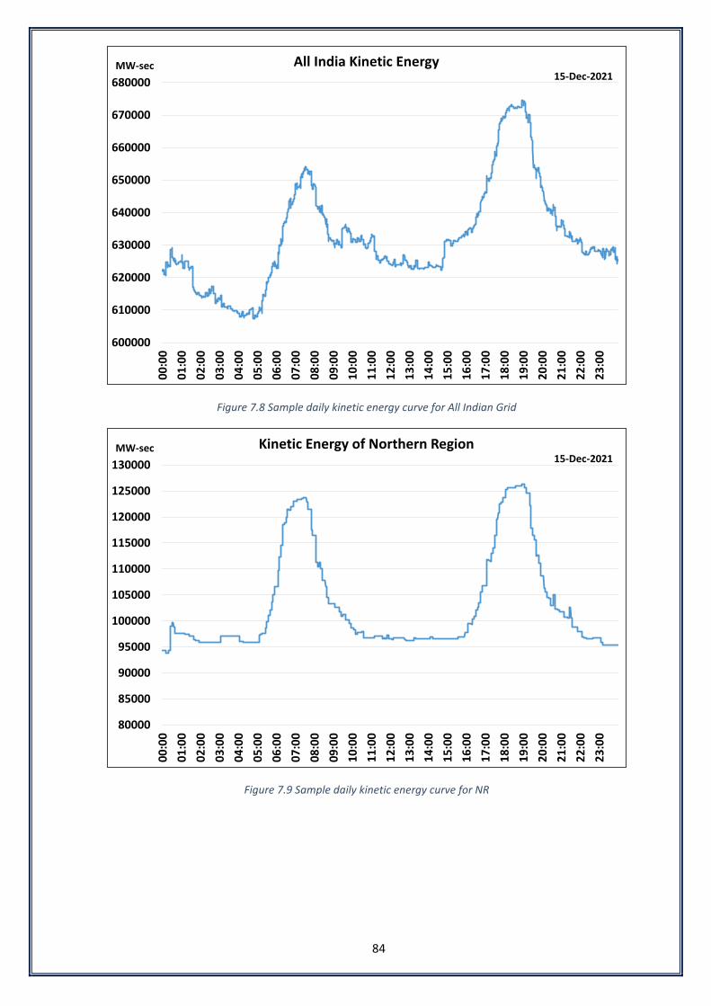
84

Figure 7.8 Sample daily kinetic energy curve for All Indian Grid

Figure 7.9 Sample daily kinetic energy curve for NR

600000

610000

620000

630000

640000

650000

660000

670000

680000

00:0

001

:00

02:0

003

:00

04:0

005

:00

06:0

007

:00

08:0

009

:00

10:0

011

:00

12:0

013

:00

14:0

015

:00

16:0

017

:00

18:0

019

:00

20:0

021

:00

22:0

023

:00

All India Kinetic EnergyMW-sec15-Dec-2021

80000

85000

90000

95000

100000

105000

110000

115000

120000

125000

130000

00:0

001

:00

02:0

003

:00

04:0

005

:00

06:0

007

:00

08:0

009

:00

10:0

011

:00

12:0

013

:00

14:0

015

:00

16:0

017

:00

18:0

019

:00

20:0

021

:00

22:0

023

:00

Kinetic Energy of Northern RegionMW-sec15-Dec-2021

85

Figure 7.10 Sample daily kinetic energy curve for WR

Figure 7.11 Sample daily kinetic energy curve for SR

200000

205000

210000

215000

220000

225000

230000

00:0

001

:00

02:0

003

:00

04:0

005

:00

06:0

007

:00

08:0

009

:00

10:0

011

:00

12:0

013

:00

14:0

015

:00

16:0

017

:00

18:0

019

:00

20:0

021

:00

22:0

023

:00

Kinetic Energy of Western RegionMW-sec15-Dec-2021

140000

145000

150000

155000

160000

165000

170000

00:0

001

:00

02:0

003

:00

04:0

005

:00

06:0

007

:00

08:0

009

:00

10:0

011

:00

12:0

013

:00

14:0

015

:00

16:0

017

:00

18:0

019

:00

20:0

021

:00

22:0

023

:00

Kinetic Energy of Southern RegionMW-sec15-Dec-2021

86

Figure 7.12 Sample daily kinetic energy curve for ER

Figure 7.13 Sample daily kinetic energy curve for NER

142000

143000

144000

145000

146000

147000

148000

149000

150000

151000

00:0

001

:00

02:0

003

:00

04:0

005

:00

06:0

007

:00

08:0

009

:00

10:0

011

:00

12:0

013

:00

14:0

015

:00

16:0

017

:00

18:0

019

:00

20:0

021

:00

22:0

023

:00

Kinetic Energy of Eastern RegionMW-sec15-Dec-2021

0

2000

4000

6000

8000

10000

12000

00:0

001

:00

02:0

003

:00

04:0

005

:00

06:0

007

:00

08:0

009

:00

10:0

011

:00

12:0

013

:00

14:0

015

:00

16:0

017

:00

18:0

019

:00

20:0

021

:00

22:0

023

:00

Kinetic Energy of North Eastern RegionMW-sec15-Dec-2021

87

Chapter 8: Frequency Response Characteristics in Indian Power System

8.1 Primary Frequency Response Requirement Post inertial response which is the first and inherent response to a frequency event, the primary frequency response is the first stage of the automated frequency control in a power system which restricts/limits the overall frequency deviation after a disturbance, bringing it to a nadir/zenith point. Once the system frequency deviates from a predefined band, the primary frequency response would typically start within a few seconds from the start of the frequency event. The speed of response depends on the resource mix which is in operation at a point in time. The primary frequency response of a system is measured in MW/Hz.

Power systems are designed and operated so as to withstand the sudden loss/connection of an identified quantum of generation/loads without posing a threat to frequency stability. The system inertia helps in controlling the immediate rate of change of frequency post an event. Inertial response and primary frequency response helps to limit the deviation in frequency before frequency is restored to steady state through despatch of secondary (automatic) and tertiary reserves (manual).In case of inadequate inertial and primary response the frequency would continue to decline and could potentially lead to the loss of load through the triggering of automatic under frequency based load shedding scheme (AUFLS). Primary frequency response from thermal (210 MW and above), gas (50 MW and above), and hydro generating units (25 MW and above) is mandated in IEGC.

8.2 Estimation of Frequency Response Indicators Frequency measurements from different locations of the Indian power system for various disturbances have been collected and analysed to investigate the overall system inertia. The frequency response indicators are calculated for each frequency disturbance. It is important to note that frequency does not remain same throughout the system during system dynamics. Propagation of synchronizing torque throughout the system can also be visualized using a snapshot of measured frequency shown in Figure 8.1. The selection of measurement node location for assessing the frequency behaviour during the disturbance is of prime importance. A sample plot for the frequency behaviour at different locations in the grid for a disturbance involving a loss of around 1000 MW of generation is provided in Figure 8.1.

88

Figure 8.1 Frequency behaviour at different locations across the grid for generation loss event The frequency response parameters/indicators can help assess the frequency response for the various disturbance selected for analysis. The various frequency indicators, as described in section 2.3, have been used in analysing the frequency response in Indian grid. Figure 2.4 provides a graphical representation of the different frequency response indicators during a disturbance.

The analysis was carried out for the last 30 events in Indian grid from Jan 2018, the value of ΔF was plotted against the quantum of generation/Load loss. The regression analysis was carried out to understand a potential linear correlation between the two parameters, the value of R2 =1 indicates perfect correlation and the value of R2 =0 indicates that two quantities are not at all linearly related with each other. As observed in Figure 8.2, the two parameters are inter-related with R2 = 0.6025. A similar plot was drawn for generation/load loss against fraction of the loss w.r.t. total system demand as shown in Figure 8.3, having R2 as high as 0.73.

89

Figure 8.2 Maximum frequency deviation vs. power imbalance

Figure 8.3 Maximum frequency deviation vs. normalized power imbalance

90

On comparing the results in Figure 8.2 and Figure 8.3, it can be inferred that maximum frequency deviation is having better correlation with load/generation loss as a fraction of total load than simple quantum of load/generation loss. The improvement in R2 values indicate that maximum frequency deviation has better correlation with system load. The system load is an approximate indicator of kinetic energy of the system i.e inertia.

8.2.1 Time to reach Nadir/Zenith Frequency The time to reach Nadir/Zenith Frequency is another important indicator of system inertia and primary frequency response. It is a good indicator of the strength of the system to resist the change in frequency. It is observed worldwide that low inertia systems experience high ROCOF values and extreme nadir/Zenith values. If the time to reach nadir frequency is low then it does not give much time for the primary responsibility to act. Time to reach frequency nadir/zenith in Indian grid for the selected list of the events is plotted in Figure 8.4. It can be observed that average time to reach frequency extreme in Indian grid is around 10 s.

Figure 8.4 Observed time to reach nadir frequency during events

8.2.2 Steady-State frequency deviation Steady state frequency in Indian grid can be referred as the quasi-steady state frequency achieved post the disturbance and deployment of primary frequency response. The available frequency data of the events indicate that frequency stabilizes in around 50 seconds from the start of the disturbance. However, the value of such frequency response parameters may change along with the integration of more RE based generation. The steady state frequency deviation signifies the

91

rate at which the primary response is activated after a disturbance. The parameter has been plotted against the generation loss/load loss during the events as given in Figure 8.5.

Figure 8.5 Magnitude of steady state frequency deviation against the event generation/load loss

8.2.3 Frequency Response Characteristic Power system oppose any sudden change in the system frequency, whereby loads typically respond in direct proportion to the frequency change, and generations respond in inverse proportion. The combined regulation by load and generation is an indication of the strength of the system in terms of frequency regulation. In the absence of any external factors such as load shedding, the system will achieve a new steady-state point after a disturbance has taken place. However, immediately following a disturbance, the frequency starts decelerating/accelerating towards a transient minimum/maximum deviation point, where the frequency decline/rise is arrested, also known as frequency nadir/zenith. The frequency response characteristics of the Indian power system [calculated as per the procedure (https://posoco.in/frc) approved by the Central Electricity Regulatory Commission] for incidents of load/generation loss is given in Figure 8.6. It can be inferred from the plot that regulation strength has improved from 4000 MW/Hz to 15000 MW/Hz in Jan 2015 to January 2021. This improvement can be attributed to increased system size and enhanced primary frequency response. It is to be noted that the component of primary frequency response is also considered in the calculation as it comes into operation within 2-4 seconds of the start of disturbance.

https://posoco.in/frc

92

Figure 8.6 Frequency Response characteristics observed during grid events in India

93

Chapter 9: RE Driven Inertia Trends and Simulation Analysis of

Indian Power System

In view of large scale RE integration in the Indian power system, it is prudent to track the variation of inertia for different timeframes. One of the ways to derive total system inertia/kinetic energy in a regional power system or Indian power system is to use the expected generation mix and basic assumptions about the inertia constant and loading factor for each generation technology. In this regard, the Western region of Indian power system was chosen for the study. Future regional scenarios identified for scheduling and dispatch for the year 2022 are used to assess the impact of the changes ongoing and foreseen on the kinetic energy in the system.

9.1 Effect of RE capacity on inertia The total electric demand in the system minus wind and solar generation represents the net load met with dispatchable sources including imported electricity from outside the system. During high RE penetrations, synchronous generators may remain offline for economic reasons, which reduces system inertia. Dispatch pattern of synchronous generators are influenced by both system load and by the amount of non-synchronous (wind and solar) generation in the system. System inertia, therefore, is correlated with net load (total demand minus the aggregated wind and solar generation). A linear correlation between system inertia and net load has been assumed in the analysis reported in this section.

System Inertia = a*Net Load +b

9.1.1 Variation of WR Kinetic Energy

Figure 46 shows the scatter plot of the total kinetic energy of the Indian Power system w.r.t the renewable penetration for the years 2017 to 2019 and 2022. For estimation of kinetic energy during 2017 to 2019, the historical data has been used. For 2022, estimation has been done using the anticipated 8760 hour optimal dispatch/unit commitment arrived at in Greening the Grid study [23].

94

Figure 9.1 Variation of WR kinetic energy wrt RE Penetration

It can be observed from Figure 9.1, that in the year 2022 the total variation in kinetic energy values is higher than in 2019 due to increase in renewable penetration. The minimum values of kinetic energy in 2022 are lower than in 2019, and the maximum values are higher than in the year 2019 which can be attributed to higher number of conventional plants online. Figure 9.2 shows the box and whisker plot for the total kinetic energy for the years 2017 to 2019 and 2022. Each boxplot representing one year facilitates an easy comparison.

Figure 9.2 Estimated Kinetic Energy of Western Region

95

Kinetic energy duration plots are shown in Figure 9.3. Right from the year 2017 to 2019, kinetic energy of the western region is above 190 GWs for 100% of the time, which drops below 190 GWs in 2022 for 20% of the time and at times it is even below 180 GWs for small duration of time. Table 9.1 provides year wise statistics of estimated Kinetic Energy.

Figure 9.3 Duration Curve of Kinetic Energy

Table 9.1 Year wise statistics of estimated Kinetic Energy

Year KE Mean (MW.sec)

KE Median (MW.sec)

KE Min (MW.sec)

KE Max (MW.sec)

2016 193140 192769 176678 210840 2017 208453 208983 193758 221005 2018 220979 220823 204469 239568 2019 240935 242858 222916 256466 2022 224404 224187 178615 265541

9.1.2 Variation of WR Online synchronous generation capacity

Online synchronous generation capacity varies with the renewable generation penetration. As extended synchronization of units and maintaining technical minimum schedules is not economical, synchronization and desynchronization of synchronous units is likely to take place frequently under high RE scenarios. The online synchronous generation capacity and aggregate power generation in the western region w.r.t renewable penetration for the year 2017 to 2019 and 2022 is shown in Figure 9.4 and Figure 9.5 respectively. As expected, it can be observed that the online capacity reduces with increase in renewable penetration. Similarly, in line with online capacity, online generation also

96

reduces w.r.t renewable penetration and in year 2022 it can be expected that large number of conventional units may operate at technical minimum.

Figure 9.4 Online synchronous capacity of Western Region wrt RE penetration

Figure 9.5 Synchronous generation of Western Region wrt RE penetration

The box plots of online synchronous generation capacity and their power generation over the years are depicted in Figure 9.6 and Figure 9.7. The online generation capacity having increasing trend even in year 2022 due to maximisation of generation from online capacity can be attributed to increased demand as well.

97

Figure 9.6 Online synchronous capacity of Western Region over the years

Figure 9.7 Synchronous generation of Western Region over the years

98

9.2 Simulation studies using all India model In India, the frequency control continuum presently encompasses inertial response followed by governor response, automatic generation control, and RRAS. AGC is in continuous operation since July 2021. Presently, around 50 GW capacity is wired under AGC. RRAS is in operation since April 2016. An all India simulation model has been developed in MATLAB/SIMULINK to predict the frequency nadir, rate of change of frequency and quasi steady state frequency following a contingency. A lumped inertia model is assumed for representing the all India inertial response. For AGC, each region is considered as a control area and all the generators under AGC are modelled with respective droop characteristics (3-6%). All other generators in the grid are lumped together with a droop of 5%.

In the practical model (Figure 9.8), the following simulation components have been considered to analyze the effects of inertia, frequency sensitive load, primary response, secondary frequency control (AGC) on system frequency followed by contingency: Load model, governor model, turbine model, droop characteristics of generators, AGC (PID controller), capacity & ramp rates, dead band zones and limiters have been modelled for comprehensive understanding of frequency control and future use post completion of AGC implementation in Indian grid.

The derivation of a power system dynamic model and carrying out simulation-based study is important to identify the degree of stability and response of power system to the identified credible contingencies. A simulation based study carried out for Indian power system has been detailed in later part of this section.

The scope of the simulation results presented in this report is limited to the inertia and primary response time frame (few milliseconds to few seconds). In the model, H is the combined generator inertia constant in seconds for the Indian power system. D is the load contribution to frequency, expressed as percentage change in load per percentage change in frequency. It has been shown in Chapter 4 and 6, that the inertia of Indian power system can somewhere be estimated broadly between 5s - 9s. However, for the purpose of simulations, there are no readily available numbers for the estimates of H and D.

99

Figure 9.8 Multi‐Region integrated Frequency Control model

Figure 9.9 Governor and Turbine model

The governor and turbine are modelled as simple first order low pass filters, 1/ (1+sTg) and 1/ (1+sTt) respectively where Tg is the governor time constant, and Tt is the turbine time constant (Figure 9.9). Tg and Tt have been assumed as 0.8s and 10s for the infinite bus grid, considering the mix of large generators in the Indian power system that has large thermal (subcritical and supercritical), hydro and Combined Cycle Gas Turbine (CCGT) power plants amongst others.

The model has been tuned and validated using the frequency response observed in 26 grid events. The data from the disturbances for the period of March 2020 to Nov 2021 is captured through PMU with a sampling rate of 25 samples per second. The list of events is shown in Table 9.2.

100

Table 9.2 List of grid events for the period of March 2020 to Nov 2021 Event Date Description

1 01-Mar-20 Generation loss around 1340 MW at NJPC & Rampur & Karcham

2 19-Mar-20 JPL stage -II station tripped. Generation loss in the event was 1139 MW

3 28-May-20 Generation loss of 5346 MW observed Sasan Vindhyachal complex

4 11-Jun-20 Generation loss of around 2126MW at Bhadla(PG) & Bhadla (Rajasthan)

5 14-Jul-20 Koyna Hydro power plant causing generation loss of around 975MW 6 20-Jul-20 At Amarsagar, wind generation loss of around 1213 MW occurred 7 22-Jul-20 Solar generation loss at Bhadla Rajasthan 1402 MW 8 16-Jul-20 Teesta generation loss during an event, 1394 MW 9 06-Aug-20 At Akal, wind generation loss of around 1348 MW occurred 10 13-Aug-20 At Jhakri, Karcham and Rampur, generation loss 1200 MW occurred

11 12-Oct-20 In the partial blackout of Mumbai incident, total load loss occurred was 2600MW and generation loss was around 840MW. FRC has been calculated for load relief of 1540 MW.

12 26-Dec-20 At Wanakbori station, the total generation loss occurred was 1011 MW. 13 19-Feb-21 1300 MW Solar generation loss at Bhadla PG

14 10-Mar-21 Multiple trippings occurred in Sikkim generation complex. The total generation loss was 1507 MW.

15 24-Mar-21 Multiple trippings occurred at Bhadla generation complex. The total net generation loss was 1586 MW.

16 8-Apr-21 Multiple Units tripped at Tuticorin Thermal Power station (TTPS). The total generation loss was 1045 MW.

17 11-Jun-21 Multiple trippings occurred at Akal wind complex. The total generation loss was 1500 MW.

18 20-Jul-21 Multiple trippings occurred at Akal wind complex. The total generation loss was 1550 MW.

19 22-Jul-21 Multiple Units tripped at UPCL (Units 1 & 2) and VARAHI Hydro (Units 1,2,3, & 4). The total generation loss was 1400 MW.

20 6-Aug-21 Unit I & II of SEIL tripped. The total generation loss was 1235 MW.

21 15-Aug-21 Multiple trippings occurred at Bhadla generation complex. The total net generation loss was 1100 MW.

22 22-Aug-21 Karcham Wangtoo units tripped on Bus bar protection. The total net generation loss was 1080 MW.

23 26-Aug-21 Multiple trippings occurred at Bhadla & Fatehgarh generation complex. The total generation loss was 1740 MW.

24 28-Sep-21 Smelter loads at Vedanta plant tripped. The load loss in the event was 1535 MW.

25 21-Oct-21 Teesta III units tripped. The total generation loss was 1086 MW.

26 15-Nov-21 Multiple trippings occurred at Bhadla generation complex. The total generation loss was 1787 MW.

101

Parameter estimation for H and D values has been manually tuned to match the resulting simulated frequency following a simulated load-generation imbalance, to visually match the PMU frequency data (ROCOF, Nadir and Quasi Steady State) for all the above mentioned 26 events. The range of the values (as already established in the earlier chapters) has been observed to be between 6s-9s for inertia and 2%-5% per Hz for load frequency sensitivity. With that informed background, tuning was done. Governor droop of 5% has been assumed for primary frequency response for all the generators, so the quasi-steady state frequency simulation represents more of an ideal situation. The value of inertia in seconds which provided the best fit is 11 seconds on 105 MVA base. After converting H to the demand MVA base during that particular instant, the H value is plotted in Figure 9.10. Taking an average value of H = 7 seconds for the Indian power system yields a decent match for nadir frequency during the events.

Figure 9.10 Inertia assumed for the 26 events to arrive at the validation plots

Load frequency sensitivity is assumed as D= 2.75 on 105 MVA base to arrive at the best possible match. On an actual demand MVA base, D = 1.8 (average value) has been arrived as shown in the Figure 9.11. That means, 1 Hz change in frequency will lead to 3.6% change in frequency sensitive load in the Indian power system.

4

5

6

7

8

9

10

1 2 3 4 5 6 7 8 9 10 11 12 13 14 15 16 17 18 19 20 21 22 23 24 25 26

Seco

nds

Event Number -->

Inertia (s)

102

Figure 9.11 Load frequency sensitivity assumed for the 26 events to arrive at the validation plots

Therefore, consideration of H=7 seconds and D=1.8 can be assumed in the simulation for a fair approximate of the Indian power system simulation model in order to match the frequency response parameters (nadir and RoCoF). Using the above data, reference contingency of 4500 MW generation loss has been simulated. Output of the model suggests that that Nadir frequency during such an event will be 49.55 Hz (if the pre-contingency frequency is 50 Hz) and quasi steady state frequency will be 49.71 Hz. The system frequency for this case is given in Figure 9.12.

Figure 9.12 System frequency after reference contingency event of 4500 MW perturbation

1

1.2

1.4

1.6

1.8

2

2.2

1 2 3 4 5 6 7 8 9 10 11 12 13 14 15 16 17 18 19 20 21 22 23 24 25 26

Load Frequency Sensitivity

Nadir = 49.55 Hz

Quasi Steady State = 49.71 Hz

103

9.3 Summary Impact analysis of RE penetration on system inertia considering estimated RE penetration for the year 2022 has been carried out. The inertia and kinetic energy trends indicate that there is declining trend in synchronous inertia and rotating mass (kinetic energy) for higher RE penetration scenarios.

The developed simulation model can estimate the RoCoF and frequency nadir/zenith with a good degree of accuracy accurately for contingencies (generation loss/load loss) in the system. The main inputs to this simulation model are the load-generation imbalance of any expected event in MW and the initial frequency. The model will be further improved for higher accuracy. Any future events can be used for validation and improvement of this simulation model.

105

Chapter 10: Recommendations and Way Forward

A detailed review of power system inertia estimation/measurement/monitoring techniques and international practices of inertia estimation, followed by inertia estimation/monitoring in Indian grid and related analysis has been carried out in this study. This initial study on power system inertia estimation/measurement in Indian grid has provided broader, yet critical insights for secure and stable grid operation of All India grid under high RE penetration. The study also helped in identifying the necessary steps required to strengthen the existing inertia monitoring platform implemented at NLDC and RLDCs and highlighted the potential technical and regulatory/policy interventions that can be taken up by the respective stakeholders to ensure secure grid operation.

Based on the conclusions derived from this study, a set of recommendations categorized in the two baskets, technical and policy/regulatory recommendations are summarized below.

10.1 Technical Recommendations: 1. Maintaining power system inertia adequacy should be included in the overall planning of

system security. Maximum Rate of change of Frequency threshold values and corresponding system inertia requirement should be considered, particularly for higher RE penetration levels.

2. Advanced, yet easy to implement inertia estimation/measurement/forecasting tools are required for accurate estimation, measurement and forecast of synchronous inertia.

3. Looking forward to the RE targets in Indian grid for the years 2022, 2030 and beyond, frequency response from the demand side, including behind-the-meter generation, is likely to play an important role in maintaining RoCoF and frequency nadir/zenith adequacy. Therefore, it is important to have a better understanding of the load composition and variation in load composition (over the week days, weekends, during peak and off-peak load, and across different seasons). This activity will require a coordinated effort from various stakeholders, particularly DISCOMS, State and the National system operators, and system regulators.

4. For RoCoF measurement, an adequate time window should be arrived at and used in RoCoF measurement across the grid. A measurement window of around 120-500 ms is generally being used across different utilities in different countries. While 500 ms appears to be more appropriate time window for averaged RoCoF measurement, further technical analysis along with the stakeholder discussion can help in arriving at standardizing the RoCoF measurement in Indian grid.

5. RoCoF and Frequency nadir based UFLS schemes, need to be revisited periodically and adopted to account for changing grid characteristics due to increased RE penetration. A similar approach may be adopted for RoCoF and under/over frequency protection settings for generating units, however, this would need closer stakeholder consultation to factor technical limitations of the existing generation fleet and cost implications that may arise

106

due to retrofitting requirements potentially required to adopt the generating units to higher RoCoF limits.

6. Minimum synchronous inertia required for secure and stable grid operation under high RE penetration should be explored for Indian grid. Since, the existing inverter-based resources (IBRs) are primarily grid following, potential non-synchronous inertial response from such sources is unlikely to influence the maximum RoCoF the system will experience following a generation/load loss. However, grid forming converters are being foreseen to provide relatively faster inertial response compared to grid following converters, yet whether the non-synchronous inertial response from such sources would be able to match the synchronous inertial response from the conventional generating units needs to be studied [24][25][26].

7. The indicators of frequency control need to be closely monitored. The reference contingency in the Indian power system shall be updated from time to time with the augmentation of new elements. The primary frequency response of the respective control area needs to be monitored by all utilities for each event involving a sudden frequency change. The results so obtained need to be discussed in the forum and any shortfall to be reported and investigated.

8. A right balance of spatial distribution of inertia among different regional grids/frequency control areas should be ensured as the RoCoF values experienced by the system for a given contingency varies across the system depending on the location of the contingency and inertia in the nearby area.

9. Synchronous inertia requirements could be considered as one of the constraints in the future Security constrained unit commitment scheme.

10.2 Regulatory and Policy Recommendations: 10. The system inertia adequacy assessment should be made integral part of the power

system planning and operation.

11. Time window for RoCoF measurement and RoCoF limits for various protection schemes should be standardized. A framework for periodic revision of such limits due to increased RE penetration should be adopted and implemented in Indian grid.

12. Adequate and accurate inertia measurement/estimation/forecast would require sufficient and highly accurate data from various stakeholders including DISCOMS, generation utilities and other related agencies. Therefore, a regulatory intervention to ensure successful and coordinated effort from different stakeholders is likely to play an important role in realizing the objective of accurate inertia monitoring in the Indian grid. This would become more important as distributed energy resources and energy storage systems get added behind the meter.

13. For secure and stable grid operation, there is a need to study further the grid support services provided by inverter-based resources (including technologies such as grid forming inverters, BESS). As these technologies evolve and the understanding improves, suitable

107

regulatory mandates/incentivization for providing these services could be considered as the RE penetration increases beyond a certain threshold.

14. Inertial response from IBRs is likely to play an important role in FFR, particularly under high RE penetration level. Therefore, provision of inertial response capability from IBRs should be explored further and potentially introduced in grid code regulations [27].

15. Stationary and particularly mobile storage (electric vehicles) is expected to increase significantly over the next decade and beyond. Therefore, provision of frequency support, such as potential FFR, Primary and secondary frequency support from such sources can be encouraged through appropriate policy and regulatory interventions.

16. A joint effort may be undertaken to revise/modify grid code regulations/technical standards to incorporate related technical definitions, standardize RoCoF measurements, provision of inertial response control capability from IBRs, inertia estimation/measurement/forecast, and new (voluntary) frequency support ancillary service products, such as FFR.

17. Transnational synchronous interconnections leading to a larger footprint would help in increasing system inertia

18. In a net-zero scenario envisaged by 2070, generation technologies such hydro (including pumped hydro), nuclear, biomass, green hydrogen fired gas turbines, and thermal generation with carbon capture & sequestration need to be kept on the radar in view of inertia requirements.

108

Bibliography

1. E.W. Kimbark, S.B. Crary, “Power System Stability”, Wiley, 1995. 2. European Network of Transmission System Operators for Electricity (ENTSO-E). Future System Inertia

(Nordic Report), https://docstore.entsoe.eu/Documents/Publications/SOC/Nordic/Nordic_report_Future_System _Inertia.pdf

3. P. M. Ashton, C. S. Saunders, G. A. Taylor, A. M. Carter and M. E. Bradley. "Inertia Estimation of the GB Power System Using Synchrophasor Measurements". IEEE Transactions on Power Systems, vol. 30, no. 2, pp. 701-709, March 2015.

4. T. Inoue, H. Taniguchi, Y. Ikeguchi and K. Yoshida, "Estimation of power system inertia constant and capacity of spinning‐reserve support generators using measured frequency transients". IEEE Transactions on Power Systems, vol. 12, no. 1, pp. 136-143, Feb. 1997

5. Du P, Matevosyan J. “Forecast system inertia condition and its impact to integrate more renewables”. IEEE Trans. Smart Grid 2018; 9(2):1531–3.

6. ENTSO-E. Fast frequency reserve – solution to the Nordic inertia challenge. 2019. Accessed 08/02/2021. [Online]. Available: https://www.statnett.no/globalassets/for-aktorer-i-kraftsystemet/utvikling-av-kraftsystemet/nordisk-frekvensstabilitet/ffr-stakeholder-report_13122019.pdf

7. North American Electricity Reliability Corporation (NERC), “Essential Reliability Services: Whitepaper on Sufficiency Guidelines”, December 2016. [Online]. Available: https://www.nerc.com/comm/Other/essntlrlbltysrvcstskfrcDL/ERSWG_Sufficiency_Guideline_Report.pdf

8. "Inertia requirements and shortfalls," Australian Energy Market Operator, 2018. [Online]. Available: https://www.aemo.com.au/

9. "RoCoF Alternative & Complementary Solutions Project: Phase 2 Study Report," EIRGRID and SONI. [Online]. Available: https://www.eirgridgroup.com/

10. R. Rome, “‘Sonar of the power grid’: New inertia measurement tools planned for Great Britain’s electricity system,” National grid ESO. Dec 2020. [Online]. Available: https://www.nationalgrideso.com/news/sonar-power-grid-new-inertiameasurement-tools-planned-great-britains-electricity-system

11. “All India Electricity Statistics (General Review) 2021”. Central Electricity Authority (CEA). April 2021. [Online]. Available: https://cea.nic.in/wp-content/uploads/general/2020/General_Review_2021.pdf

12. “Report 1: Fundamentals of electric vehicle charging technology and its grid integration”, [Online: https://www.niti.gov.in/sites/default/files/2021-09/Report1-Fundamentals-ofElectricVehicleChargingTechnology-and-its-Grid-Integration_GIZ-IITB.pdf]

13. Thomas Ackermann. “Wind Power in power Systems”. Wiley. 2005. 14. P. M. Ashton, G. A. Taylor, A. M. Carter, M. E. Bradley and W. Hung, "Application of phasor

measurement units to estimate power system inertial frequency response," 2013 IEEE Power & Energy Society General Meeting, Vancouver, BC, 2013, pp. 1-5.

15. M. AbolhasaniJabali and M. H. Kazemi, "Estimation of inertia constant of Iran power grid using the largest simulation model and PMU data," 2016 24th Iranian Conference on Electrical Engineering (ICEE), Shiraz, 2016, pp. 158-160.

https://docstore.entsoe.eu/Documents/Publications/SOC/Nordic/Nordic_report_Future_System_Inertia.pdf




https://www.statnett.no/globalassets/for-aktorer-i-kraftsystemet/utvikling-av-kraftsystemet/nordisk-frekvensstabilitet/ffr-stakeholder-report_13122019.pdf



https://www.nerc.com/comm/Other/essntlrlbltysrvcstskfrcDL/ERSWG_Sufficiency_Guideline_Report.pdf

https://www.nerc.com/comm/Other/essntlrlbltysrvcstskfrcDL/ERSWG_Sufficiency_Guideline_Report.pdf

https://www.aemo.com.au/

https://www.eirgridgroup.com/

https://www.nationalgrideso.com/news/sonar-power-grid-new-inertiameasurement-tools-planned-great-britains-electricity-system

https://www.nationalgrideso.com/news/sonar-power-grid-new-inertiameasurement-tools-planned-great-britains-electricity-system

https://cea.nic.in/wp-content/uploads/general/2020/General_Review_2021.pdf

https://www.niti.gov.in/sites/default/files/2021-09/Report1-Fundamentals-ofElectricVehicleChargingTechnology-and-its-Grid-Integration_GIZ-IITB.pdf

https://www.niti.gov.in/sites/default/files/2021-09/Report1-Fundamentals-ofElectricVehicleChargingTechnology-and-its-Grid-Integration_GIZ-IITB.pdf

109

16. S. Canevese, E. Ciapessoni, A. Gatti and M. Rossi, "Monitoring of frequency disturbances in the European continental power system," 2016 AEIT International Annual Conference (AEIT), Capri, 2016, pp. 1-6.

17. Zografos, Dimitrios & Ghandhari, Mehrdad. (2017). “Power system inertia estimation by approaching load power change after a disturbance.” 1-5. 10.1109/PESGM.2017.8273824.

18. Schiffer, Johannes & Aristidou, Petros & Ortega, Romeo, “Online Estimation of Power System Inertia Using Dynamic Regressor Extension and Mixing”, IEEE Transactions on Power Systems

19. P. Wall and V. Terzija, "Simultaneous Estimation of the Time of Disturbance and Inertia in Power Systems," IEEE Transactions on Power Delivery, vol. 29, no. 4, pp. 2018-2031, Aug. 2014. doi: 10.1109/TPWRD.2014.2306062

20. Wilson, D. & Yu, J. & Al-Ashwal, N. & Heimisson, B. & Terzija, V. (2019). “Measuring effective area inertia to determine fast‐acting frequency response requirements.” International Journal of Electrical Power & Energy Systems. 113. 1-8. 10.1016/j.ijepes.2019.05.034.

21. EirGrid and System Operator for Northern Ireland (SONI), “All Island TSO Facilitation of Renewables Studies,” Tech. Rep., 2010

22. AEMO, “100 Per Cent Renewables Study Modelling Outcomes,” Tech. Rep. Jul, 2013

23. D. Palchak et al. “Greening the Grid: Pathways to Integrate 175 Gigawatts of Renewable Energy into India’s Electric Grid”, NREL, LBNL, POSOCO & USAID. June 2017.

24. “Grid Forming Inverters: EPRI Tutorial”. EPRI, Palo Alto, CA: 2020. 3002018676.

25. Sproul et al, “Grid Forming Energy Storage System addresses challenges of grids with high penetration of renewables (A case study)”, 18th Wind Integration Workshop, 2019.

26. A Roscoe et al (Siemens Gamesa), ‘Practical Experience of Operating a Grid Forming Wind Power Park and its Response to System Event,’ 18th Wind Integration Workshop, Dublin Oct 2019

27. Paul Denholm et al, “Inertia and the Power Grid: A Guide Without the Spin”, National Renewable Energy Laboratory, Tech. Rep., May 2020

28. S.K. Soonee and S.C. Saxena, “Frequency Response Characteristics of an interconnected power system – A case study of regional grids in India”, 6th International R&D Conference on Sustainable Development of Water and Energy Resources, pp 220-231, Lucknow, Feb 2007

29. “Report of Expert Group to review and suggest measures for bringing power system operation closer to National Reference Frequency (Vol. I)”, Central Electricity Regulatory Commission, Nov 2017

110

Annexure-1: Inertia Constant of Generators Region wise

Figure A1.1 Inertia Constant of Northern Region Generators

Figure A1.2 Inertia Constant of Western Region Generators

111

Figure A1.3 Inertia Constant of Southern Region Generators

Figure A1.4 Inertia Constant of Eastern Region Generators

112

Figure A1.5 Inertia Constant of North Eastern Region Generators

113

Annexure-2: Synchronous Condensers

Introduction

A synchronous condenser (SC) is a well-known technology introduced around 80-90 years back. The voltage control capabilities of SCs were relatively common at the transmission level during that time. However, SCs got outcompeted in terms of reactive power compensation by the power electronics devices such as Static Var Compensators (SVC) and STATCOM, these static reactive power devices have low maintenance level because they have no rotating parts. However, the SC has experienced increasing interest due to their multiple capabilities in keeping a stable power system in addition to reactive power compensation. Due to the presence of available rotating parts, SCs have the advantage of providing inertia. The facility to provide inertia coupled with reactive support has made SCs an obvious choice for systems with high RE penetration. It is thus possible to build a new SC or retrofit a decommissioned power plant generator as SC instead of shutting it down and thereby potentially take an economical approach. For the latter option, the reconfiguration of the generator is necessary to boost its standalone functionality for generating inductive and capacitive reactive power.

Theoretical Background

An SC is a synchronous machine running without a prime-mover, and hence the shaft is allowed to spin freely. Therefore, the theory and modelling behind an SC are the same as a synchronous machine, without the mechanical load. From this close relationship to a synchronous machine, it is understood that that the conventional power stations could be refurbished to a synchronous condenser, thereby potentially reducing initial capital cost. As stated, a synchronous condenser operates at close to zero active power as possible, it does however consume a small amount of active power from the system to cover losses.

The key element in a synchronous condenser is the ability of controlling the field excitation, as the level of excitation determines if the synchronous condenser generates or consumes reactive power. Another important element is the voltage control, by use of a voltage regulator a synchronous condenser can automatically regulate the reactive power output to keep a constant terminal voltage. Further elaborations on these follows in the upcoming subsections. Construction

i. Excitation System: The capabilities of the excitation system of any synchronous machine can be visualized from both a machine as well as system perspective. From a machine perspective, the intent of the excitation system is to provide and adjust the field current, so that the terminal voltage of the generator/condenser is maintained. Whereas, from a power system perspective, the intent of the excitation system is to contribute to effective voltage control and thus enhancing the system stability. As mentioned, a synchronous condenser can either consume or produce reactive power. This quality is controlled by the excitation system of the synchronous condenser, if overexcited hence leading power factor, it supplies reactive power and if under-excited hence lagging power factor, it consumes reactive power from the system. The two kinds of AC excitation systems used are given below:

114

a. Brushless excitation System: The rotating rectifier solution is also known as the brushless excitation solution, because the need for slip rings and brushes are eliminated. These can be avoided by the applying rotating rectifiers as the DC output then can be directly feed to the main generator field.

b. Static excitation system: In a static excitation system all the components are stationary, which entails that the static rectifier supplies the excitation current directly through slip rings to the field of the main generator.

ii. Decoupled Turbine: With the prime mover turbine no longer necessary for SC, it is decoupled from the generator provided the generator would no longer be used for power generation. However, a shaft extension and bearing are often used to replace the earlier turbine-generator connection for better stability. A connection through a clutch is also a viable option. If the SC operation is temporary and is followed by the regular power-generating operation in the machine, altering the connection is not required. During the retrofitting, it is essential to check other auxiliary components such as the oil supply systems and the foundation and adapt them to the updated operating mode if necessary. A new start-up mechanism must be devised and implemented to start the SC since the turbine can no longer power it into action. Generally, a simple pony motor, primarily small induction motors with a start-up variable frequency drive (VFD), will suffice for this purpose.

iii. Static Frequency Control: SFC is used to start-up the machine, and since the turbine is not available, it leads to overspeeding of the machine. An overspeeding of about 10% of the rated speed is acceptable—this further aids in identifying the rotor position and the subsequent start-up procedure. Typically, the SFC is powered from the grid. Once the machine starts overspeeding, the SFC can be switched off, followed by the synchronization of the generator with the grid during the fall-back to synchronous speed.

iv. Cooling System:

An oil circulation system is needed in SC for lubrication, cooling and bearing shaft jacking for start-ups and shutdowns if the boundary bearing conditions for lubrication happen to be below 1000 RPM. The pony motor-driven startups also get aided by the jacking oil. It is necessary to have some redundancy in the oil pumps, filters and coolers, with the DC motor-driven pumps acting as backup for the AC motor-driven pumps for start-ups and shutdown procedures.

The external cooling system for the SC will require a cooling water circuit, which would preferably be fully enclosed with circulating water pumps, closed cooling towers, a make-up supply tank and chemical dosing. The circuit would be serving the condenser air cooler elements and the oil coolers.

The complete construction diagram design is given as Figure A2.1 (Source: GE digital energy, Synchronous Condenser Systems).

115

Figure A2.1 Assembly diagram showing synchronous condenser

Conversion of existing synchronous generators into synchronous condensers:

As many gas and coal-based synchronous generators approach the end of their life, plant owners face a challenge to upgrade or retire a plant. The retiring of a plant can possibly create a reactive power deficit at the local network, which may impact voltage reliability. There will always be a gap in reactive support required to be filled once the plant is retired. The solutions of FACTS-based devices have been used, but the conversion of the existing generator to a synchronous condenser i can be potentially economical and effective one, particularly, if its multiple benefits of reactive power support, short circuit power and inertia contribution are counted in together.

There are many benefits to this conversion – the various parts of a synchronous generator can be reused like network connection, auxiliaries, prime mover and building. The synchronous condenser can produce typically about 30 percent more reactive power than what is possible in normal power generation overexcited mode.

The condition of the existing generator shall be assessed so that if the expected lifespan is more, the replacement of stator, rotor windings and excitation can be considered for enhanced output.

The important components of conversion are given below:

i. Means of starting: The synchronous condenser needs to undergo acceleration to synchronise with the grid. As no turbine is present to accelerate the condenser, synchronous or induction motors are used to play the same role.

116

ii. Prime Mover: There are two options for removing the turbine, the first being the removal of the turbine from its foundation or decoupling it. Decoupling the turbine while keeping it in place has been proven to be the better option since it causes minimal disruption in the lubrication system of the turbine-generator assembly. If desired, it also allows the condenser to be transformed back to the generator mode and vice versa.

iii. Excitation System: It is imperative to evaluate the current excitation system to check whether it can reliably deliver the required excitation current required for the rated reactive power generation. The excitation system and generator should operate at a field-current corresponding to the nameplate power factor to achieve maximum generation.

iv. Mechanical System: The components in this system are designed and installed to support the condenser rotor adequately. It consists of a thrust bearing and a turning gear on the rotor’s collector end. The lubricating oil system can also be modified in some instances to include high-pressure lift oil that reduces the breakaway torque of the rotor during start-up.

v. Control System: For controlling the start-up sequence, the excitation system, and synchronization to the grid, a new supervisory control system is fabricated and installed in place. The system is also supposed to monitor the existing protection systems, the breakers, auxiliary systems, and condenser status of the generator. It should also be unified with the overall plant controls to enable monitoring of the status of the complete system.

Footprint & Practical Considerations:

A synchronous condenser's overall footprint comprises the core device and a balance-of-plant system to connect it to the grid. The footprint size is relatively small and may not be an issue in rural areas where generally renewable rich generation is there. The sample rating of 225 MVAR synchronous condenser land requirements is shown in Figure A2.2. The noise produced by the synchronous condenser should also be considered if it is being planned somewhere near the urban settings. Enclosing the synchronous condensers inside the building may be advantageous in terms of environmental protection, sound/heat, corrosion etc.

The scale and weight of synchronous condensers may limit the locations where they can be transported to. The components are manufactured overseas and generally transported via ships; however, after landing, it depends on the capability of road and transport to carry the device to location. Therefore, it is expected that additional cost and time could be incurred on the entity. The synchronous condensers are different kinds of machines and may require significant lead times (12-24 months). The operators need to plan the generation accordingly. Once the synchronous generator is placed, it is also necessary to understand the impact of unplanned extended outages of it on renewable generation. The inclusion of a synchronous condenser in the network is expected to increase the short circuit levels. Therefore, its placement becomes important in respect of switchgear ratings.

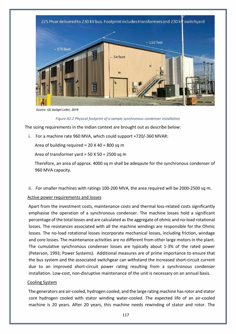
117

Figure A2.2 Physical footprint of a sample synchronous condenser installation

The sizing requirements in the Indian context are brought out as describe below:

i. For a machine rate 960 MVA, which could support +720/-360 MVAR:

Area of building required = 20 X 40 = 800 sq m

Area of transformer yard = 50 X 50 = 2500 sq m

Therefore, an area of approx. 4000 sq m shall be adeqaute for the synchronous condenser of 960 MVA capacity.

ii. For smaller machines with ratings 100-200 MVA, the area required will be 2000-2500 sq m.

Active power requirements and losses

Apart from the investment costs, maintenance costs and thermal loss-related costs significantly emphasise the operation of a synchronous condenser. The machine losses hold a significant percentage of the total losses and are calculated as the aggregate of ohmic and no-load rotational losses. The resistances associated with all the machine windings are responsible for the Ohmic losses. The no-load rotational losses incorporate mechanical losses, including friction, windage and core losses. The maintenance activities are no different from other large motors in the plant. The cumulative synchronous condenser losses are typically about 1-3% of the rated power (Peterson, 1993; Power Systems). Additional measures are of prime importance to ensure that the bus system and the associated switchgear can withstand the increased short-circuit current due to an improved short-circuit power rating resulting from a synchronous condenser installation. Low-cost, non-disruptive maintenance of the unit is necessary on an annual basis.

Cooling System

The generators are air-cooled, hydrogen cooled, and the large rating machine has rotor and stator core hydrogen cooled with stator winding water-cooled. The expected life of an air-cooled machine is 20 years. After 20 years, this machine needs rewinding of stator and rotor. The

118

machine windings have a very good thermally conductive insulation system, which keeps the thermal stress on winding low during sudden variation of MVAR during operation. Hydrogen cooled machines have been giving an excellent performance as the rate of insulation ageing is very low in these machines. The insulation of winding, being in a hydrogen environment, does not age due to increased temperature (thermal stress) as oxidation processes do not take place inside the machine. The electrical stress on winding is also very low due to increased hydrogen pressure. The machines are designed for 3kV/mm BDV. In contrast, at rated hydrogen pressure, the BDV is increased to 10kV/mm and thus, a machine experience lower electrical stress (same as 1/3rd rated voltage in air medium). Partial discharge activity in a hydrogen cooled generator is negligible. In a hydrogen-cooled machine, the leading cause of ageing is limited to mechanical ageing due to vibration or rubbing of adjacent bars. Therefore, it has been seen that winding insulation generally does not deteriorate even after 40 years of operation in most of the machines. Hydrogen cooled machines are safe, and explosion is not possible as the machines are at high hydrogen pressure 4.0-6.0 kg/cm2 and air from outside cannot enter into the machine. In the past 30 years, two cases of hydrogen leakage from seals have been reported due to turbine blade failure resulting in damage to hydrogen seals. However, Synchronous condenser machines run without any turbine. The hydrogen cooling system also has a hydrogen purging facility to send hydrogen directly outside the building whenever any maintenance is planned on the machine.

Overload Capability:

The blueprints of modern synchronous machines (including synchronous generators) not only allow them to be built reliably with fewer poles and faster speeds but also to be engineered with considerable overload capability. With a synchronous condenser, current up to 175% of nameplate rating is potentially feasible for a ten-minute duration. A current equal to up to three times the rated value can be generated for five seconds. Since most power system events are recorded in milliseconds, a ten-minute or even a five-second characteristic can be beneficial in using a synchronous condenser for dynamic support in the grid.

Source of Inertia (Flywheel addition)

SCs have been in existence since 1930 for the production of dynamic VARs (both inductive and capacitive) for enhancing the system stability and voltage support during changing load scenarios and contingencies. A voltage regulator maintains its magnetic field to either generate or absorb reactive power as required to regulate the voltage of the power system. A synchronous condenser is essentially a rotating machine without a prime mover connected to it. This is the reason behind its low inertia provision from the kinetic energy stored in the rotating mass. The typical H values of an SC range from 1-3 s. Thus, the available inertial energy in the SC can be estimated using the appropriate approach.

High-inertia synchronous condensers are recommended in order to reduce the size or number of condensers required for the installation as well as prevent system collapse due to frequency decay. High-inertia synchronous condensers can be attained either by de-rating the nameplate of a given synchronous condenser or increasing the spinning mass of the machine with the addition of a flywheel. Both the methods for increasing the inertia are evident from the following equation:

119

𝐻𝐻 =1

2� 𝐽𝐽𝜔𝜔02

𝑉𝑉𝑉𝑉𝑏𝑏𝑚𝑚𝑚𝑚𝑒𝑒

Where H is inertia constant, J is the moment of inertia of the condenser rotor, ω0 is the angular speed in radians/second, and VAbase is the nameplate rating of the machine. The inertia constant is directly proportional to machine inertia and also directly proportional to the square of machine speed. Higher speed machines will tend to be smaller in physical size for a specified electrical rating. To achieve an inertia constant significantly higher than that inherent to a machine sized only for the electrical rating, oversizing the machine is likely to be a costlier approach than considering the use of a flywheel. Depending on the speed of the machine, the flywheel geometry will change subject to mechanical stress and possibly rotational dynamic limitations. Additionally, as the flywheel inertia increases, the ability of the synchronous condenser to be self‐starting also needs to be considered, and it may become necessary to employ power electronics for this purpose. A four-pole 50 MVAr condenser design based on synchronous motor technology will have inherent inertia constant of approximately 2. When connected to a separately supported external flywheel having an inertia constant of four, an overall factor of six is achieved.

Comparison of performance with STATCOM

i. A STATCOM without an additional energy storage system cannot contribute to frequency stability, unlike a synchronous condenser. It cannot generate any reactive power if the voltage drops considerably.

ii. The standard V/Q characteristic for a STATCOM and a synchronous condenser with identical nominal ratings: The impedance of the transformer that connects both the devices must be considered when the nominal rating at the Point of Common Coupling (PCC at transformer primary side) is specified. The impedance of a synchronous condenser measured at the transformer primary side is usually 10 – 15 % lower than the nameplate rating of the synchronous machine itself. The maximum current limits the output of the STATCOM through the converter, and it can deliver the identical (symmetrical) amount of inductive and capacitive reactive power proportional to the system voltage (solid blue line). Additionally, providing more than rated current is feasible, typically 125% for 3 seconds.

iii. Unlike STATCOM, the synchronous condenser output (reactive power generation and consumption) is not symmetrical. The maximum inductive production is restricted by end region heating or small-signal stability. It usually is around 60% of the nominal rating and directly proportional to the square of the system voltage. An essential edge of a synchronous condenser is the capacitive overload capability, depending on the machine type. It is an instance of thermal overload and thus exponentially decreases with the time, typically 200% for 10 seconds or 150% for 30 seconds.

iv. The STATCOM can move from any quasi-steady-state point to another in less than two cycles. The typical time constants permit the synchronous condenser to shift its operational mode from zero MVAR to full capacitive or inductive MVARs in 1-3 seconds.

v. The STATCOM is blocked during severe two- or three-phase short-circuit faults when the positive-sequence voltage falls below a particular threshold and is de-blocked when this fault is cleared. It subsequently supports the system recovery. Synchronous condensers react to

120

sudden voltage drop similar to a relatively slowly adjustable voltage source behind a reactance. Thus, it can generate current instantly after a voltage variation is detected in the system, depending on the variation magnitude.

vi. Active power losses in STATCOM vs Synchronous Condenser: The primary share of STATCOM total losses happens in the converter and consists of power electronic switching, conducting losses, and DC capacitors losses. The remainder is made up of a transformer, reactor and auxiliary losses. Only transformer no-load and auxiliary losses are present with a zero current output.

The machine losses play a significant role in the cumulative synchronous condenser losses and are calculated as the sum of the ohmic and no-load rotational losses. Ohmic losses result from the resistances associated with all machine windings, whereas mechanical losses, including friction, windage and core losses, constitute no-load rotational losses.

References:

1. “Managing system strength during the transition to renewables,” Tech. Rep., GHD Advisory, 2020

2. J. P. Skliutas et al “Planning the Future Grid with Synchronous Condensers”. CIGRE US National Committee. 2013 Grid of the Future Symposium

3. Y. Liu, S. Yang, S. Zhang and F. Z. Peng, "Comparison of synchronous condenser and STATCOM for inertial response support," 2014 IEEE Energy Conversion Congress and Exposition (ECCE), 2014, pp. 2684-2690, doi: 10.1109/ECCE.2014.6953761.

4. S. Teleke, T. Abdulahovic, T. Thiringer and J. Svensson, "Dynamic Performance Comparison of Synchronous Condenser and SVC," in IEEE Transactions on Power Delivery, vol. 23, no. 3, pp. 1606-1612, July 2008, doi: 10.1109/TPWRD.2007.916109.

5. “Addressing the system strength gap in SA ‐ Economic Evaluation Report”, Electranet, Feb 2019

6. S. Kynev, G. Pilz and H. Schmitt, "Comparison of modern STATCOM and synchronous condenser for power transmission systems," 2016 IEEE Electrical Power and Energy Conference (EPEC), 2016, pp. 1-6, doi: 10.1109/EPEC.2016.7771769.

7. “Synchronous Condenser Systems”, Product brochure, GE Digital Energy

Power System Operation Corporation Limited (A Government of India Enterprise) | CIN: U40105DL2009GOI188682

B-9, Qutab Institutional Area, New Delhi – 110016

www.posoco.in | [email protected]

Assessment of Inertia in Indian Power System - POSOCO

Documents

Transcript of Assessment of Inertia in Indian Power System - POSOCO