The role of inertia in models of the geodynamo

Geophys. J. Int. (2004) 158, 515–528 doi: 10.1111/j.1365-246X.2004.02369.x

GJI

Geo

mag

netism

,ro

ckm

agne

tism

and

pala

eom

agne

tism

The role of inertia in models of the geodynamo

D. R. Fearn and M. M. Rahman∗Department of Mathematics, University of Glasgow, Glasgow G12 8QW, UK. E-mail: [email protected]

Accepted 2004 May 12. Received 2004 April 28; in original form 2003 October 3

S U M M A R YNumerical studies of the geodynamo have taken different views on the importance of inertialeffects. Some have neglected inertia, while others have boosted its strength, in much the sameway as they have had to take an artificially high viscous force because of numerical consider-ations. Yet others have taken an intermediate view. In terms of the standard non-dimensionalnumbers, the Ekman number E measures the strength of viscous effects, the magnetic Ekmannumber Eη measures the strength of inertia, and the magnetic Prandtl number P m = E/E η.Virtually all studies have P m ≥ 1 (E η ≤ E), even though geophysical values give P m 1. Those studies that have undertaken parameter surveys have found no dynamo action whenP m < P mc, where Pmc is an O(1) number that depends on E. We have therefore been motivatedto undertake a systematic study of the effect of inertia. In order to work with a manageableproblem, we have used a non-linear mean-field dynamo driven by an α-effect [α = α0 cos θ

sin π (r − r i)]. In this, a finite-amplitude field drives a flow through the Lorentz force in themomentum equation, and this flow feeds back on the field-generation process in the magneticinduction equation, equilibrating the field. This equilibration process is a key aspect of thefull hydrodynamic dynamo. What we are not modelling here is the effect on convective-drivenprocesses of changes in inertia; our forcing α-effect is fixed considered the system in the ab-sence of inertia. Here, we include the full inertial term. For an Ekman number of E = 2.5 ×10−4, we have investigated dynamo solutions for the magnetic Ekman number in the rangeE η = 5.0 × 10−5 to 9.0 × 10−2 (corresponding to reducing Pm from 5 to ∼0.003). In thisrange we find three distinct types of solution. At the higher values of Pm we find solutions verysimilar to those found in the absence of inertia. The addition of inertia damps out the rapidtime dependence found in its absence. The major effect we have found is that the addition ofinertia (decreasing Pm) facilitates dynamo action; for a given level of forcing (i.e. fixed α0),increasing Eη results in an increased amplitude of the magnetic (and kinetic) energy. Thereis no shut-off of dynamo action with decreasing Pm as found in hydrodynamic models. Thisdifference gives an insight into the various aspects of the dynamo process. By focusing onthe field-generation process, using a fixed α that is independent of Eη, we have shown thatinertia modifies the flow driven by the Lorentz force in a manner that is beneficial to fieldgeneration. The contrast between the present mean-field model and the results of hydrody-namic models shows that the effect of inertia on the driving process (thermal convection) isdetrimental to field generation, more than compensating for the beneficial effect identifiedhere.

Key words: inertia, mean-field dynamo, non-linear dynamo.

1 I N T RO D U C T I O N

The past decade has seen major developments and increased ac-tivity in the study of the geodynamo, spurred on by new observa-

∗On leave from Department of Mathematics, University of Dhaka, Dhaka-1000, Bangladesh.

tions and computational developments. The ground-breaking workof Glatzmaier & Roberts (1995a,b) has encouraged an increasingnumber of groups to develop their own numerical models (see forexample Christensen et al. 2001). In such models a number of non-dimensional parameters must be prescribed. These typically dependon material properties, such as the viscosity or the electrical con-ductivity of the core. While our knowledge of these properties isimproving (see for example Alfe et al. 2002; de Wijs et al. 1998),

C© 2004 RAS 515

Dow

nloaded from https://academ

ic.oup.com/gji/article/158/2/515/770177 by guest on 28 M

ay 2022

516 D. R. Fearn and M. M. Rahman

there remains considerable uncertainty in the exact geophysical val-ues of many quantities. Furthermore, in numerical models, there areconstraints on the values of some parameters that are currently ac-cessible. The most significant of these constraints is on the Ekmannumber

E = ν

0 L2, (1)

where ν is the kinematic viscosity, L is a characteristic length scale,here taken to be the width ro − r i of the outer core, and 0 is therotation frequency of the mantle. Using the molecular value of theviscosity, in the Earth E = O(10−15). In numerical models, res-olution constraints mean that typically E is taken no smaller thanO(10−4), or perhaps O(10−5). Clearly this is very far from the geo-physical value and any uncertainties in the viscosity of the coreare currently essentially irrelevant as far as numerical modelling isconcerned.

The low value of E suggests that one approach is simply to neglectthe effect of viscosity altogether. This approach has been successfulfor magnetoconvection problems, but has so far failed for the hy-dromagnetic dynamo problem (see for example Walker et al. 1998).As a result, all successful hydromagnetic geodynamo models haveincluded viscous effects.

Another important parameter is the magnetic Ekman number

Eη = η

0 L2, (2)

where η is the magnetic diffusivity. In the core, Eη is of the order of10−9. This gives a measure of the relative strength of inertial termsin the Navier–Stokes equation determining the evolution of the coreflow. [The quantity defined in eq. (2) is sometimes referred to asthe Rossby number Ro. Strictly speaking Ro = U/0 L , where Uis a characteristic speed, and the two quantities match only whenU = η/L .]

Motivated by the smallness of Eη, some numerical models ofthe geodynamo neglect inertial terms altogether, a few choose thegeophysical value, while many take the view that Eη should be nosmaller than the Ekman number. The magnetic Prandtl number

Pm = E/Eη = ν/η (3)

is small in the core, but the numerical constraints on E mean thatmost numerical models take P m ≥ O(1). Taking the geophysicalvalue of Eη while accepting the numerical constraints on E im-plies a large magnetic Prandtl number, while neglecting inertialeffects altogether corresponds to the infinite magnetic Prandtl num-ber limit. Whatever the choice, almost all studies choose a fixedvalue of Eη and focus on other aspects of the problem. Very littlework has focused specifically on the role of inertia in the dynamoproblem.

Given the numerical constraints on E, there is no ‘correct’ choicefor Eη. What is clear, though, is that there is a need for a sys-tematic survey in which the value of Eη is varied in order to de-termine the influence of inertia on the geodynamo problem. Al-though fully 3-D models are available, they are computationallyhighly intensive. In these circumstances, we believe that furtherinvestigations using simpler models are appropriate, and we havechosen to use a mean-field α2-dynamo model. These models havelower computational requirements and so are useful for a parametersurvey and for developing our understanding of the role of inertiaon geodynamo solutions. Such an approach is also very useful inthat it complements hydrodynamic dynamo studies. The choice ofa mean-field model with prescribed α means that we are focusing

on the effect of inertia on the field-generation process. The influ-ence of inertia on the convection, which is here parametrized bythe α-effect, is, of course, not modelled. We discuss this further inSection 6.

In computational models we need to accept values of E that arevery much larger than the geophysical value. For the magnetic Ek-man number we are free from such a constraint. By setting E η =0 rapid fluctuations associated with the rotational timescale are fil-tered out, making solutions easier to obtain. If the inertial term is tobe included, the fact that E is larger than its geophysical value mustalso affect the choice of Eη. In the Earth’s core, the viscous timescalecan be as short as O(E1/2), while the rotational timescale is O(Eη).For the lowest manageable values of E, the rotational timescale willbe shorter than the viscous timescale. Therefore the choice of Eη

depends on any assumption that is made for the relative size of thesetimescales.

The first Earth-like magnetic field was generated by Glatzmaier& Roberts (1995a,b) using a 3-D global model designed to simulatethe core. Inertial effects were neglected. These models included onlythermal buoyancy and used the Boussinesq approximation. Theirlater models (Glatzmaier & Roberts 1996a,b,c, 1997, 1998) includedthe axisymmetric part of the azimuthal component of the inertiaand accounted for both thermal and compositional buoyancy, usingthe anelastic approximation. They prescribed E = 10−6 (achievedusing hyperdiffusivities), E η = 10−9, and adopted no-slip boundaryconditions for the flow. There are significant differences betweenthe earlier and later models, but since the difference between themis not limited to the addition of inertia it is not possible to identifyto what extent changes in the solutions are due to inertia. Giventheir choice of P m = 103, it seems likely that the effect of inertia isweak.

Kuang & Bloxham (1997, 1999) developed a Boussinesq modelthat used different velocity and thermal boundary conditions fromGlatzmaier & Roberts and also produced an Earth-like magneticfield outside the core. Their model incorporated all components ofthe axisymmetric inertia. They were able to minimize the viscoustorque on the Taylor cylinders by imposing stress-free boundaryconditions. At the outer core boundary, their strong-field dynamosolution for E η = E = 2 × 10−5 is similar to the observed geo-magnetic field in many aspects: the field is dominantly dipolar anddrifts westwards. Inside the fluid core, their solution differs greatlyfrom the solutions of Glatzmaier & Roberts. The field in the Kuang& Bloxham solution is dominantly generated in the bulk of the fluidcore outside the tangent cylinder, while the field in the Glatzmaier& Roberts dynamo solution is generated near the inner core bound-ary and inside the tangent cylinder. Kuang & Bloxham (1997) havedemonstrated that, when a strong viscous coupling is introducedon the boundaries while the inertia is kept unchanged, the dynamosolutions undergo a transition from Kuang & Bloxham’s solutionto solutions qualitatively the same as the Glatzmaier & Roberts dy-namo solutions.

Proctor (1977) studied an α2-dynamo in a full sphere includingall components of inertia. He examined the equilibration processof the evolved magnetic field. The form of α was simple: α =α0 cos θ . The values of E and Eη that he studied are E = 1.0,0.01, 0.005 and E η = 1.0, 0.01, 0.025. For E = 0.005 and E η =0.0025 he noticed the occurrence of persistent oscillations for allvalues of α0. As he changed the values of both E and Eη at thesame time, it is not clear how inertia alone affected the solution.Jault (1995), using an αω-dynamo model, found that restoring justthe axisymmetric part of the inertial term can help to prevent thephysical and numerical instabilities associated with small viscosity.

C© 2004 RAS, GJI, 158, 515–528

Dow



ay 2022

Inertia and models of the geodynamo 517

Fearn & Morrison (2001, hereafter referred to as FM) investigatedthe role of inertia in hydrodynamic models of the geodynamo. Inorder to permit a reasonable survey of parameter space, they usedthe so-called 2.5-D model (Jones et al. 1995; Sarson et al. 1998;Morrison & Fearn 2000). This uses full resolution in radius r andcolatitude θ but is highly truncated in azimuth φ. The computationalrequirements of the 2.5-D model are much lower than those of fully3-D models. In their calculations they used E/2 = 10−3 and Eη/2in the range 5 × 10−5 to 5 × 10−4. (Note: the definitions of E andEη used by FM differ by a factor of 2 from those adopted here.)As Eη is increased from zero, their solutions show evidence of asmooth transition from the inertia-less solution until E η/2 ≈ 10−4,where there is a transition to a new, higher-amplitude solution. Thelower-Eη solution has a time dependence that is periodic, while thelarger-Eη solution is more chaotic. Increasing Eη further results ina decreasing solution amplitude, and above E η/2 ≈ 5 × 10−4 (P m

below ∼2) no dynamo solutions were found.Fearn & Rahman (2004, hereafter referred to as FR) (see also Rah-

man 2003) gave mean-field dynamo solutions in a rapidly rotatingspherical shell with a finitely conducting inner core and insulatingmantle. Inertial effects were again neglected. The velocity boundaryconditions they imposed were no-slip at the boundaries. The formof α chosen was α = α0 cos θ sin π (r − r i). For this α they gavesolutions for the Ekman number in the range E = 5 × 10−5 to E =2.5 × 10−3. FR investigated a rapid time behaviour which suggeststhat the effects of inertia may not be negligible. Here, we want toinvestigate this problem further, with inertial effects included, andto undertake a parameter survey of solution behaviour as a functionof Eη. The mean-field model is simpler than the convectively drivenmodel of FM, permitting exploration of a wider range of magneticEkman number, Eη.

The organization of the remainder of the paper is as follows. InSection 2 we describe our physical model with governing equa-tions and boundary conditions, and in Section 3 discuss the solutionmethod very briefly. In Section 4 we discuss the role of inertia on ourα2-dynamos. Finally, in Section 5 we summarize our results beforepresenting our conclusions in Section 6.

2 P H Y S I C A L M O D E L

The model we are investigating consists of a spherical shell of innerradius r i and outer radius ro that is rotating about its axis with angu-lar velocity = 0ez , where ez is the unit vector in the z-direction.The region r i ≤ r ≤ r o is filled with an electrically conductingfluid of constant kinematic viscosity ν, magnetic diffusivity η, mag-netic permeability µ and density ρ 0. The exterior region r ≥ r o iselectrically insulating, to model the Earth’s mantle. The fluid andits interior region have the the same electrical conductivity, σ (andη = 1/µσ ). The governing non-dimensional equations for the evo-lution of the magnetic field and fluid flow based on the scales: length,L = r o − r i; time, τ η = L2/ η; fluid velocity, U = η/L; magneticfield, B = (0µρ0η)1/2 and pressure, P = 0 L2/τη are as follows.In the fluid outer core:∂B

∂t= ∇ × (u × B + αB) + ∇2B, (4)

Eη

[∂u

∂t+ (u.∇)u

]+ 2ez × u − E∇2u

= −∇ P + (∇ × B) × B, (5)

∇.u = 0, (6)

where B is the magnetic field, u is the fluid velocity, P is the pressure,and α is the α-effect, chosen to be

α = α0 cos θ sin π (r − ri). (7)

In the finitely conducting inner core, we solve

∂B

∂t= ∇ × (ui × B) + ∇2B, (8)

where ui = ir sin θeφ with i = iez denoting the inner coreangular velocity. Here we have used B to represent the magneticfield in the inner core.

The non-dimensional parameters appearing in (5) are defined in(1) and (2). For all the calculations in this paper, we have used E =2.5 × 10−4 and a spherical shell with radius ratio r i/r o = 1/3.Values of the magnetic Ekman number Eη in the range 5 × 10−5

−0.09 have been investigated. The problem has been looked at indetail by FR for the case E η = 0. They found the onset of dynamoaction for α0 = 6.69, and transition to the ‘spiked’ behaviour at α0 ≈10.8. We have investigated a variety of values of α0 up to α0 = 12,but our main results are for α0 = 10 and α0 = 11.

Our model is axisymmetric. The α-effect term in (4) is a well-established way (see, for example, Moffatt 1978) of representingthe mean electromotive force due to the non-linear interaction ofthe non-axisymmetric parts of the field and the flow.

There is no current in the mantle as it is electrically insulating,so the boundary condition for the field at the core–mantle boundary(CMB) becomes

B = B(e) at r = ro, (9)

where B(e) is the external potential field. We are also considering afinitely conducting inner core, so at the inner core boundary (ICB)the field in the outer core and field in the inner core will match:

B = B, at r = ri. (10)

For the flow we impose no slip at the boundaries. The boundarycondition for the flow at the CMB becomes

u = 0 at r = ro. (11)

Since the inner core is rotating with an angular velocity i, theno-slip velocity boundary condition at the ICB becomes

u = ir sinθeφ at r = ri. (12)

A freely rotating finitely conducting inner core has a stabilizingeffect on the dynamo solution (Hollerbach & Jones 1993, 1995).This finitely conducting inner core couples electromagnetically withthe outer core, giving rise to a magnetic torque on the inner core.The equation that determines the angular velocity of the inner core,i, is the torque balance on the inner core (Glatzmaier & Roberts1996c; Aurnou & Olson 2000):

C Eη

∂i

∂t= E

∫S

r∂

∂r

(uφ

r

)|r=riri sin θ d S

+∫

SBr Bφ |r=riri sin θ d S, (13)

where C = (8/15)πr 5i (considering an inner and outer core of equal

density).

3 C A L C U L AT I O N S

The numerical method that we are using for our calculation is basedon the code developed by Hollerbach (2000). He used a pseudospec-tral method to solve the magnetoconvection equations in a spherical

C© 2004 RAS, GJI, 158, 515–528

Dow



ay 2022


Figure 1. Contour plots of (left to right) B, Ar sin θ , v/r sin θ and ψr sin θ at (top to bottom) α0 = 7, 8, 9, 10 (cf. fig. 1 of FR) for E η = 10−4, E = 2.5 ×10−4. Contour intervals are 0.2, 0.02, 4 and 0.04 respectively. Solid lines represent positive contours, and dashed lines represent negative contours.

C© 2004 RAS, GJI, 158, 515–528

Dow



ay 2022


geometry. Hollerbach (2000) used a decomposition of B and u intopoloidal and toroidal parts:

B = ∇×Aeφ + Beφ, u = ∇×ψeφ + veφ (14)

(Bullard & Gellman 1954), as they automatically satisfy thesolenoidal conditions ∇.B = ∇.u = 0. He further used KB Cheby-shev polynomials in the radial direction and LB spherical harmonicsin the θ -direction. The time-stepping procedure was implementedvia a second-order Runge–Kutta predictor–corrector method, mod-ified to treat the diffusive terms implicitly. Further details are givenin Rahman (2003).

With inertia included, the momentum equation (5) as well as thetorque balance equation (13) are time-stepped to update the fluidvelocity u and the angular velocity Ωi via the terms E η∂u/∂t andE η∂ i/∂t . This approach is clearly not possible when E η = 0 (seeJones et al. 1995; Morrison & Fearn 2000; FR; Rahman 2003). Thenumerical method of this paper is therefore not capable of exploringE η = 0 solutions, but lower values of E η ≤ 10−4 give results veryconsistent with E η = 0. FR have calculated solutions correspondingto E η = 0 for different values of α0 and E = 2.5 × 10−4. Fig. 1 showscontour plots of B (toroidal field strength), Ar sin θ (poloidal fieldlines), v/rsin θ (differential rotation) and ψr sin θ (poloidal flowstreamlines) for α0 = 7, 8, 9, 10 and E η = 10−4, E = 2.5 × 10−4.In these cases, although we did not impose any symmetry constraintabout the equator, we found steady dipole solutions. The strengthof the field and flow increase with increasing α0. Comparing thestructure of these solutions with the E η = 0 solution, fig. 1 of FR,we found almost exact agreement for both the field and the flow,indicating that, at this value of Eη, inertial effects are having at mosta modest effect on the problem.

The numerical scheme involves a time-stepping calculation ofthe spectral coefficients. Energies are calculated, as required, fromthese spectral coefficients and are a useful measure for monitoringthe solutions. In a typical calculation, the system is allowed to marchforwards in time until the evolved magnetic field has settled downto a finite amplitude. The magnetic energy that we calculate is

E∗M = 1

2µ

∫v1

|B∗|2 dv

= [ρ00ηL3

] (1

2

∫v1

|B|2 dv

)= [

ρ00ηL3]EM, (15)

where v1 is the computational domain and B∗ is the dimensionalfield. Similarly, the kinetic energy that we calculate is

E∗K = ρ0

2

∫v2

|u∗|2 dv

= [ρ00ηL3

] (1

2Eη

∫v2

|u|2 dv

)= [

ρ00ηL3]

EK, (16)

where v2 is the volume of the outer core and u∗ is the dimensionalfluid velocity.

The value of E that we have chosen (E = 2.5 × 10−4) is one ordersmaller than that used by FM. The magnetic Ekman number E η =10−4 represents a reasonable starting point for our calculations andis relatively high [compared with the geophysical value of O(10−9)]so that we can employ a sensible time step to resolve in time. We haveperformed calculations for various values of Eη, with the full rangeinvestigated given in Tables 1 and 2. The choice of time step dependson the choice of Eη. As we vary the magnetic Ekman number, Eη,we find the structure of the solution may require higher truncation toresolve it properly. Therefore, the level of truncation also dependson Eη.

Table 1. Magnetic energy EM for various values of Eη at α0 = 10, 11.

EM

Eη α0 = 10 α0 = 11

0 6.42 3.92–81.165 × 10−5 6.50 3.90–80.51

10−4 6.51 3.89–80.705 × 10−4 6.52 3.86–81.48

10−3 6.53 3.82–83.035 × 10−3 6.70 3.60–90.00

10−2 7.19 3.81–96.642 × 10−2 9.14 9.185 × 10−2 19.93 26.397 × 10−2 27.15 35.408 × 10−2 32.70 39.36

8.5 × 10−2 35.81 42.619 × 10−2 38.02 45.50

Table 2. Kinetic energy EK for various values of Eη at α0 = 10, 11.

EK

Eη α0 = 10 α0 = 11

5 × 10−5 3.8 × 10−3 1.2 × 10−3 − 0.1610−4 7.7 × 10−3 2.3 × 10−3 − 0.31

5 × 10−4 3.9 × 10−2 1.1 × 10−2 − 1.0410−3 7.7 × 10−2 2.1 × 10−2 − 1.20

5 × 10−3 0.39 9.2 × 10−2 − 8.3710−2 0.85 0.12–14.51

2 × 10−2 2.18 2.475 × 10−2 9.36 13.857 × 10−2 14.98 21.318 × 10−2 18.96 24.60

8.5 × 10−2 20.13 29.329 × 10−2 22.64 29.59

The solution corresponding to α0 = 7, E = 2.5 × 10−4, E η =10−4 was calculated from a random initial condition. After a coupleof diffusion times, the solution converged to a finite amplitude. Thesolutions corresponding to higher α0 were calculated using the α0 =7 solution as an initial condition. We found the solution for α0 =10, E = 2.5 × 10−4 and E η = 10−4, and then investigated the effectof increasing Eη.

4 R E S U LT S

To investigate the role of inertia, we calculated solutions for α0 =10 and α0 = 11 for a range of values of Eη. These are summarized inTables 1 and 2 and Fig. 2. The E η = 0 solutions are taken from FR,who used a different code. The small-Eη results clearly approachthe E η = 0 results. From Table 1 we see that the change in magneticenergy is modest up to E η ≤ 10−2. Beyond this, the change inmagnetic energy is more rapid.

FR found solutions corresponding to a range of values of α0

for E = 2.5 × 10−4 and E η = 0. While steady for low valuesof α0, these solutions developed a rapid time behaviour when α0

was increased above some critical value αp = 10.8 for E = 2.5 ×10−4. It is interesting to see how inertia affects this behaviour. Theresults of our parameter survey in Eη for α0 = 11 are summarizedin Fig. 2, which shows the variation in the amplitude of magneticenergy (top) and kinetic energy (bottom). There are three notablefeatures apparent in Fig. 2.

First, there appears to be a smooth trend, with the E η > 0 re-sults approaching the E η = 0 result as Eη is decreased. In Fig. 2,

C© 2004 RAS, GJI, 158, 515–528

Dow



ay 2022


Figure 2. Magnetic energy (top) and kinetic energy (bottom) as a function of E η = Ro for α0 = 11. Lines represent energy that is oscillatory, bullets representenergy that is steady, and squares represent the average energy of a periodic solution.

vertical lines represent the lower and upper bounds of the rapidtime-behaviour solutions. From Tables 1 and 2 we see that the upperbounds (lower bounds) of these solutions increase (decrease thenincrease) very slowly with increasing Eη. In Fig. 3, we have plotteda snapshot of the solution for E η = 10−3 and α0 = 11, to be com-pared with Fig. 1. The flow structure is clearly unchanged, althoughthe flow has a slightly higher magnitude. The structures of the fieldsin Figs 1 and 3 are similar. The field and flow structures remainunchanged qualitatively throughout the range 5 × 10−5 ≤ E η

<∼ 1.2× 10−2.

The time dependence of the magnetic energy for various values ofEη is shown in Fig. 4. The behaviour of the kinetic energy is similar to

that of the magnetic energy, and both show a similar behaviour to thecase without inertia. (See fig. 4 of FR, who discuss the nature of thisrelaxation oscillation in detail, demonstrating the strong influenceof Taylor’s constraint in the rapid growth phase, where growth isessentially at the linear growth rate.) One noticeable feature is theperiod of oscillation. Fig. 5 shows the period versus Eη for α0 = 11and E = 2.5 × 10−4. From this figure we see that the period withoutinertia (asterisk) and that with small inertia (the nearest bullet to theasterisk) are in excellent agreement. From the parameter survey byFR (see their fig. 3), we know that the period of a solution for fixedE initially decreases as α0 increases and then settles down to a finitevalue. We also know that the period goes to infinity as α0 approaches

C© 2004 RAS, GJI, 158, 515–528

Dow



ay 2022


Figure 3. Snapshot of the solution for E η = 10−3, E = 2.5 × 10−4, α0 =11. Contour plots are shown of B, Ar sin θ (top row) and v/rsin θ , ψr sin θ

(bottom row). Contour intervals are 0.2, 0.02, 4 and 0.04 respectively. Solidlines represent positive contours, and dashed lines represent negative con-tours.

the onset of oscillatory solutions (α0 = αp). Fig. 5 shows the cleareffect of inertia on the period. As Eη increases, the period decreasessmoothly as Eη increases up to E η ≤ 7.0 × 10−3. Beyond this, theperiod increases and near E η ≈ 1.2 × 10−2 it approaches infinity(i.e. a stationary solution).

The second notable feature in Fig. 2 is the evolution to a steadysolution at E η ≈ 1.2 × 10−2. Using the E η = 1.1 × 10−2 oscil-latory solution as the initial condition, we calculated the solutionfor E η = 1.2 × 10−2 and found a steady solution. Using the E η =1.2 × 10−2 solution as the initial condition, we ran the programfor E η = 1.15 × 10−2 and found the previous oscillatory solu-

tion, indicating that the nature of the bifurcation is supercritical.Similarly, using the higher magnetic Ekman number E η = 1.5 ×10−2 solution as the initial condition, we ran the program again forE η = 1.2 × 10−2 and found the same steady solution. This con-firms that at this Eη we have only one solution. The amplitudes ofmagnetic energy and kinetic energy increase with increasing Eη.These steady solutions exist in the range 1.2 × 10−2 <∼ E η

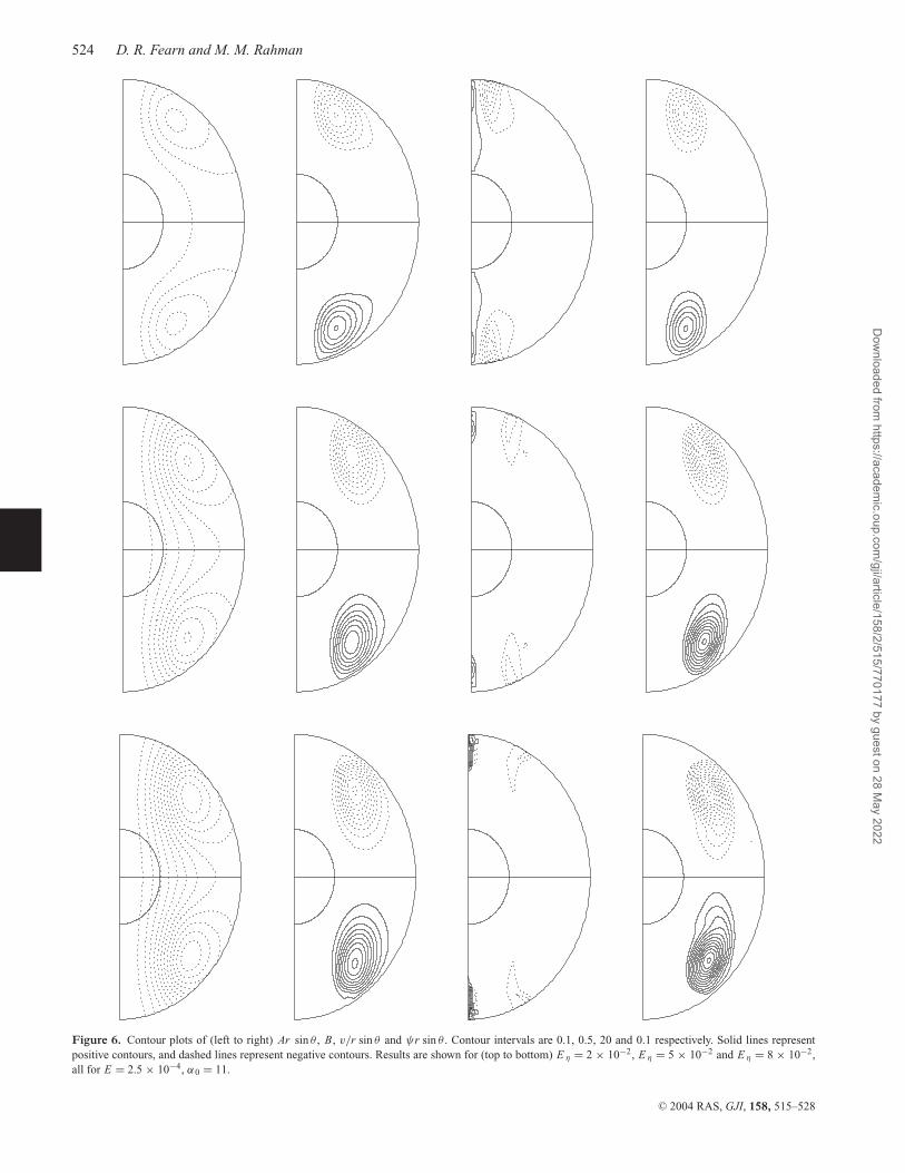
<∼ 8.5 ×10−2. Fig. 6 shows the solutions for E η = 2 × 10−2, 5 × 10−2 and8 × 10−2. As Eη increases, the toroidal field B, the poloidal fieldAr sin θ and the poloidal flow ψr sin θ increase in strength whileroughly retaining their form and moving slightly to lower latitudes.By contrast, the differential rotation v/rsin θ diminishes with in-creasing Eη. Further calculations for E = 10−4 give very similarresults.

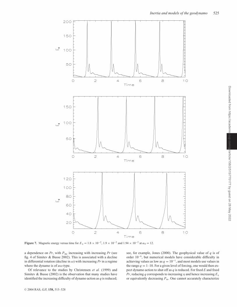
We investigated this transitional behaviour from a spiked solutionto a steady solution further for the higher value of α0 = 12 (seeTable 3). The behaviour of the period as a function of Eη showsa similar behaviour to that in Fig. 5. From Table 3 we see thatthe height of the spiked solutions falls very quickly as Eη tendsto the critical value Eη c. This is clearer from the energy plots inFig. 7 in the region of Eη c. From these figures we see that at thebottom of these spikes there appear to be several oscillatory modesthat become stronger as Eη increases and pull down the highestspike.

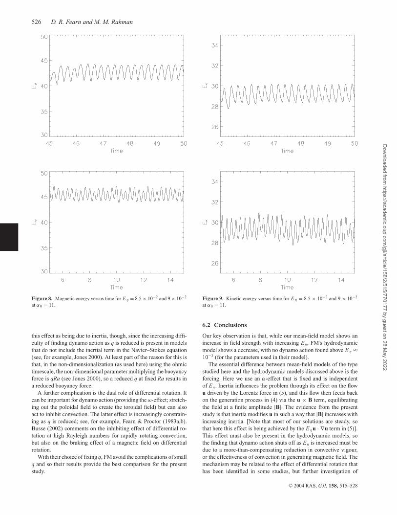
The final notable feature in Fig. 2 is the periodic solution beyondE η = 8.5 × 10−2. Figs 8 and 9 show the variation of magneticand kinetic energies over Eη in this parameter regime. Both EM

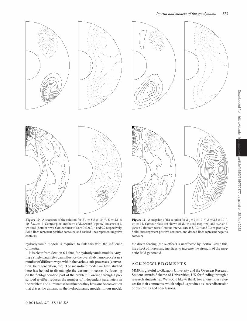
and EK oscillate in a periodic fashion for E η = 8.5 × 10−2. Wecalculated the E η = 8.5 × 10−2 solution using the E η = 8.0 ×10−2 solution as the initial condition, which took a long time tosettle down (top plots). The solution corresponding to E η = 9.0 ×10−2 oscillates quite irregularly. Fig. 10 shows snapshots of the fieldand flow for E η = 8.5 × 10−2. Comparing this with Fig. 6, we seethat both the azimuthal and meridional field have moved towardsthe equatorial plane. For the azimuthal field no activity is observedclose to the inner boundary. The structures of the angular velocityand meridional flow are now completely different. They are highlyasymmetric. A lot of activity is now observed both inside and outsidethe tangent cylinder. The angular velocity has small-scale features.Fig. 11 shows a snapshot of the same axisymmetric quantities (cf.Fig. 10) for E η = 9.0 × 10−2 after five diffusion times. The fieldand flow are now highly asymmetric and the solutions have evolvedinto a mixed mode. In Figs 10 and 11 we are clearly beginningto run into resolution problems for v/r sin θ near the axis (wherer sin θ is small). We ran the same calculations at higher resolution.The results found are the same as shown, except for minor detailsclose to the axis for v/r sin θ . Owing to the resolution difficultiesdescribed above we stopped our parameter survey here.

FM found the structure of the flow remained similar in boththeir weak-field (oscillatory) and strong-field (chaotic) branches.However, the structure of the field in their stronger-field branch iscompletely different from that in the weaker-field branch. In theweaker-field branch their field was nearly quadrupolar, while inthe stronger-field branch it was mixed mode. In our model both thefield and flow structures remain the same in the spiked and steadybranches but are different in the periodic branch. The former anddipolar and the latter is mixed mode.

A feature of FM’s convectively driven dynamo is the shut-off ofdynamo action as Eη is increased. In their solutions no dynamowas found for E η/2 >∼ 5.0 × 10−4, even when the forcing wasincreased (i.e. the Rayleigh number was increased). At E η = 5.0 ×10−4, increasing the Rayleigh number from 50 to 60 resulted in a

C© 2004 RAS, GJI, 158, 515–528

Dow



ay 2022


Figure 4. Magnetic energy versus time for E η = 10−4 (top), 10−3 (middle), 10−2 (bottom) and α0 = 11.

significantly stronger field, yet in both cases increasing Eη to E η/2 =6.25 × 10−4 resulted in failure to maintain a field. In our model weexplored a lower value of E and a wider range of Eη than FM andfound no indication of shut-off of dynamo action. We comment onthis further in Section 6, where the differences between mean-fieldand convectively driven dynamos are discussed.

The behaviour noted in Fig. 2 shows both the magnetic and kineticenergies to be roughly proportional to Eη. Given the definitions ofthe non-dimensional energies, see (15) and (16), this implies that|B| ∼ E1/2

η and |u| ∼ E0η. If we then look at the steady version of

the induction equation (4), we see that all terms are of order E1/2η ,

so the leading-order balance in this equation is independent of Eη.

C© 2004 RAS, GJI, 158, 515–528

Dow



ay 2022


Figure 5. Period versus E η = Ro for α0 = 11.

Table 3. Magnetic energy and kinetic energy for various values of Eη andα0 = 12.

Eη EM EK

0 6.07–210.37 –5 × 10−5 6.04–203.12 2.6 × 10−3–0.58

10−4 6.01–203.55 4.7 × 10−3–1.085 × 10−4 5.93–204.73 2.2 × 10−2–3.83

10−3 5.84–206.03 4.2 × 10−2–6.485 × 10−3 5.13–218.43 0.17–23.29

10−2 4.62–223.33 0.40–36.041.5 × 10−2 4.52–214.14 0.75–42.681.8 × 10−2 4.90–203.82 1.46–46.211.9 × 10−2 5.24–182.64 2.01–43.951.92 × 10−2 5.33–165.07 2.07–39.911.94 × 10−2 5.42–132.94 2.12–30.882.5 × 10−2 10.93 4.255 × 10−2 35.60 19.588 × 10−2 49.19 31.5

In the momentum equation (5), the Lorentz and inertial terms areof order Eη, with the viscous term of order E. As the strength ofEη is increased from zero (where viscous effects have a controllinginfluence), at some value of Eη inertial effects become more im-portant. Then, a balance is possible between inertia and the Lorentzforce that results in an increase in |B| with E1/2

η . In our present study,inertia is an important influence when Eη is of order 10−2, corre-sponding to P m

<∼ 0.02. How this relates to the value of E can onlybe determined by a more extensive parametric study. What is clear,though, is that the mechanism observed here becomes importantwhen Pm is small.

5 S U M M A RY

The role of inertia in a mean-field non-linear α2-dynamo has beeninvestigated using a rapidly rotating spherical shell with a finitelyconducting inner core, insulating mantle and a realistic α = α0 cos θ

sin π (r − r i) vanishing at both the inner and outer boundaries of thecore. The key non-linear effect, which acts to equilibrate dynamosolutions at finite amplitude, is the flow driven by the Lorentz force.The influence of inertia on this flow and the consequent variationin the equilibrated field strength is the main focus of this investi-gation. The value of the Ekman number that we have used is E =2.5 × 10−4. From earlier work (FR) that neglects inertial effects

(E η = 0), we know that at this value of E steady dipole solutionsexist for values of α0 < 10.8, and that oscillatory reversing spikedsolutions are found for higher values of α0. The nature of the spikedsolutions is qualitatively the same for the range of α0 (up to α0 =14) studied; for example, the period of the oscillations is essentiallyindependent of α0 for α0 > 12 (see fig. 3 of FR). Here, we considervalues of α0 up to 12, but believe that our results give the correctqualitative picture for higher forcing.

We found a smooth transition from the E η = 0 results to thosefor small Eη; thus, the addition of a small amount of inertia resultsin solutions very similar to those found in the absence of inertia. Athigher Eη, inertia has the effect of damping out the rapid (spiked)time behaviour observed at low Eη: we found steady solutions for10−2 <∼ E η

<∼ 8 × 10−2. The major effect of inertia was foundto be that it facilitates dynamo action, with the magnetic energyincreasing significantly with increasing E η (see Fig. 2). Our resultsspan a range in Eη from 5 × 10−5 to 9 × 10−2, corresponding to arange in Pm from 5 to ∼ 3 × 10−3. The lower limit on Eη and theupper limit on Pm are not significant since we found our results atthese values to essentially match the corresponding solutions foundin the absence of inertia (E η = 0 or P m → ∞).

6 D I S C U S S I O N A N D C O N C L U S I O N S

The key conclusions of this study relate to the differences betweenmean-field dynamos and convectively driven hydrodynamic dy-namos and to what insight this gives us into aspects of the dynamomechanism.

6.1 Hydrodynamic models

In hydrodynamic studies (where convection drives the field-generation process), additional parameters appear. There is theRayleigh number that measures the forcing (and so, very roughly,replaces our α0), and there is the Prandtl number

Pr = ν/κ, (17)

where κ is the thermal diffusivity. In place of the magnetic Prandtlnumber Pm, many studies thus use the Roberts number

q = κ/η = Pm/Pr. (18)

Comparisons between studies are often made difficult by the differ-ent choices made for the parameters, and in particular which are keptfixed while others are varied. For example, FM increase Eη whilstkeeping E and q fixed. This implies a corresponding decrease in thevalues of Pm and Pr.

The work by FM (which used a 2.5-D hydrodynamic model) foundthere to be no dynamo action above some value of Eη, and belowthis value there was a decrease in magnetic energy with increas-ing Eη. These observations are in agreement with other, fully 3-D,hydrodynamic calculations. Christensen et al. (1999) conducted aparametric study for fixed Pr = 1 (so q = P m, and decreasingPm at fixed E corresponds to increasing Eη). They found dynamoaction only for P m > P mc ∼ 450E3/4. For E = 10−3, P mc ∼ 2,and for E = 10−4 they found P mc ∼ 0.5. The results of FM can bere-expressed in terms of Pm. For fixed q = 10 and E/2 = 10−3, theyfind dynamo action only for E η/2 <∼ 5 × 10−4. This is equivalentto P m

>∼ 2, consistent with Christensen et al.’s results. (Note thatthe two surveys are not directly comparable since FM fix q whileChristensen et al. fix Pr.) Simitev & Busse (2002) also find dynamoaction to be more difficult to achieve as Pm is reduced. They find

C© 2004 RAS, GJI, 158, 515–528

Dow



ay 2022


Figure 6. Contour plots of (left to right) Ar sin θ , B, v/r sin θ and ψr sin θ . Contour intervals are 0.1, 0.5, 20 and 0.1 respectively. Solid lines representpositive contours, and dashed lines represent negative contours. Results are shown for (top to bottom) E η = 2 × 10−2, E η = 5 × 10−2 and E η = 8 × 10−2,all for E = 2.5 × 10−4, α0 = 11.

C© 2004 RAS, GJI, 158, 515–528

Dow



ay 2022


Figure 7. Magnetic energy versus time for E η = 1.8 × 10−2, 1.9 × 10−2 and 1.94 × 10−2 at α0 = 12.

a dependence on Pr, with Pmc increasing with increasing Pr (seefig. 4 of Simitev & Busse 2002). This is associated with a declinein differential rotation (decline in ω) with increasing Pr in a regimewhere the dynamo is of αω-type.

Of relevance to the studies by Christensen et al. (1999) andSimitev & Busse (2002) is the observation that many studies haveidentified the increasing difficulty of dynamo action as q is reduced;

see, for example, Jones (2000). The geophysical value of q is oforder 10−6, but numerical models have considerable difficulty inachieving values as low as q = 10−1, and most models use values inthe range q = 1–10. For a given level of forcing, one would then ex-pect dynamo action to shut off as q is reduced. For fixed E and fixedPr, reducing q corresponds to increasing η and hence increasing Eη

or equivalently decreasing Pm. One cannot accurately characterize

C© 2004 RAS, GJI, 158, 515–528

Dow



ay 2022


Figure 8. Magnetic energy versus time for E η = 8.5 × 10−2 and 9 × 10−2

at α0 = 11.

this effect as being due to inertia, though, since the increasing diffi-culty of finding dynamo action as q is reduced is present in modelsthat do not include the inertial term in the Navier–Stokes equation(see, for example, Jones 2000). At least part of the reason for this isthat, in the non-dimensionalization (as used here) using the ohmictimescale, the non-dimensional parameter multiplying the buoyancyforce is qRa (see Jones 2000), so a reduced q at fixed Ra results ina reduced buoyancy force.

A further complication is the dual role of differential rotation. Itcan be important for dynamo action (providing the ω-effect; stretch-ing out the poloidal field to create the toroidal field) but can alsoact to inhibit convection. The latter effect is increasingly constrain-ing as q is reduced; see, for example, Fearn & Proctor (1983a,b).Busse (2002) comments on the inhibiting effect of differential ro-tation at high Rayleigh numbers for rapidly rotating convection,but also on the braking effect of a magnetic field on differentialrotation.

With their choice of fixing q, FM avoid the complications of smallq and so their results provide the best comparison for the presentstudy.

Figure 9. Kinetic energy versus time for E η = 8.5 × 10−2 and 9 × 10−2

at α0 = 11.

6.2 Conclusions

Our key observation is that, while our mean-field model shows anincrease in field strength with increasing Eη, FM’s hydrodynamicmodel shows a decrease, with no dynamo action found above E η ≈10−3 (for the parameters used in their model).

The essential difference between mean-field models of the typestudied here and the hydrodynamic models discussed above is theforcing. Here we use an α-effect that is fixed and is independentof Eη. Inertia influences the problem through its effect on the flowu driven by the Lorentz force in (5), and this flow then feeds backon the generation process in (4) via the u × B term, equilibratingthe field at a finite amplitude |B|. The evidence from the presentstudy is that inertia modifies u in such a way that |B| increases withincreasing inertia. [Note that most of our solutions are steady, sothat here this effect is being achieved by the E ηu · ∇u term in (5)].This effect must also be present in the hydrodynamic models, sothe finding that dynamo action shuts off as Eη is increased must bedue to a more-than-compensating reduction in convective vigour,or the effectiveness of convection in generating magnetic field. Themechanism may be related to the effect of differential rotation thathas been identified in some studies, but further investigation of

C© 2004 RAS, GJI, 158, 515–528

Dow



ay 2022


Figure 10. A snapshot of the solution for E η = 8.5 × 10−2, E = 2.5 ×10−4, α0 = 11. Contour plots are shown of B, Ar sin θ (top row) and v/r sin θ ,ψr sin θ (bottom row). Contour intervals are 0.5, 0.2, 4 and 0.2 respectively.Solid lines represent positive contours, and dashed lines represent negativecontours.

hydrodynamic models is required to link this with the influenceof inertia.

It is clear from Section 6.1 that, for hydrodynamic models, vary-ing a single parameter can influence the overall dynamo process in anumber of different ways within the various sub-processes (convec-tion, field generation, etc). The mean-field model we have studiedhere has helped to disentangle the various processes by focusingon the field-generation part of the problem. Forcing through a pre-scribed α-effect reduces the number of independent parameters inthe problem and eliminates the influence they have on the convectionthat drives the dynamo in the hydrodynamic models. In our model,

Figure 11. A snapshot of the solution for E η = 9 × 10−2, E = 2.5 × 10−4,α0 = 11. Contour plots are shown of B, Ar sin θ (top row) and v/r sin θ ,ψr sin θ (bottom row). Contour intervals are 0.5, 0.2, 4 and 0.2 respectively.Solid lines represent positive contours, and dashed lines represent negativecontours.

the direct forcing (the α-effect) is unaffected by inertia. Given this,the effect of increasing inertia is to increase the strength of the mag-netic field generated.

A C K N O W L E D G M E N T S

MMR is grateful to Glasgow University and the Overseas ResearchStudent Awards Scheme of Universities, UK for funding through aresearch studentship. We would like to thank two anonymous refer-ees for their comments, which helped us produce a clearer discussionof our results and conclusions.

C© 2004 RAS, GJI, 158, 515–528

Dow



ay 2022


R E F E R E N C E S

Alfe, D., Gillan, M.J. & Price, G.D., 2002. Composition and temperatureof the Earth’s core constrained by combining ab initio calculations andseismic data, Earth planet. Sci. Lett., 195, 91–98.

Aurnou, J. & Olson, P., 2000. Control of inner core rotation by electromag-netic, gravitational and mechanical torques, Phys. Earth planet. Inter.,117, 111–121.

Bullard, E.C. & Gellman, H., 1954. Homogeneous dynamos and terrestrialmagnetism, Phil. Trans. R. Soc. Lond., A, 247, 213–278.

Busse, F.H., 2002. Convective flows in rapidly rotating spheres and theirdynamo action, Phys. Fluids, 14, 1301–1314.

Christensen, U., Olson, P. & Glatzmaier, G.A., 1999. Numerical modellingof the geodynamo: a systematic parameter study, Geophys. J. Int., 138,393–409.

Christensen, U.R. et al., 2001. A numerical dynamo benchmark, Phys. Earthplanet. Inter., 128, 25–34.

de Wijs, G.A., Kresse, G., Vocadlo, L., Dobson, D., Alfe, D., Gillan, M.J. &Price, G.D., 1998. The viscosity of liquid iron at the physical conditionsof the Earth’s core, Nature, 392, 805–807.

Fearn, D.R. & Morrison, G., 2001. The role of inertia in hydrodynamicmodels of the geodynamo, Phys. Earth planet. Inter., 128, 75–92 (FM).

Fearn, D.R. & Proctor, M.R.E., 1983a. Hydromagnetic waves in a differen-tially rotating sphere, J. Fluid Mech., 128, 1–20.

Fearn, D.R. & Proctor, M.R.E., 1983b. The stabilising role of differ-ential rotation on hydromagnetic waves, J. Fluid Mech., 128, 21–36.

Fearn, D.R. & Rahman, M.M., 2004. Evolution of nonlinear α2-dynamos and Taylor’s constraint, Geophys. astrophys. Fluid Dyn.,in press (FR).

Glatzmaier, G.A. & Roberts, P.H., 1995a. A three-dimensional convectivedriven dynamo solution with rotating and finitely conducting inner coreand mantle, Phys. Earth planet. Inter., 91, 63–75.

Glatzmaier, G.A. & Roberts, P.H., 1995b. A three-dimensional self-consistent computer simulation of a geomagnetic field reversal, Nature,377, 203–209.

Glatzmaier, G.A. & Roberts, P.H., 1996a. On the magnetic sounding ofplanetary interiors, Phys. Earth planet. Inter., 98, 207–220.

Glatzmaier, G.A. & Roberts, P.H., 1996b. An anelastic evolutionary geody-namo simulation driven by compositional and thermal convection, PhysicaD, 97, 81–94.

Glatzmaier, G.A. & Roberts, P.H., 1996. Rotation and magnetism of Earth’sinner core, Science, 274, 1887–1891.

Glatzmaier, G.A. & Roberts, P.H., 1997. Simulating the geodynamo, Con-temp. Phys., 38, 269–288.

Glatzmaier, G.A. & Roberts, P.H., 1998. Dynamo theory then and now, Int.J. Eng. Sci., 36, 1325–1338.

Hollerbach, R., 2000. A spectral solution of the magnetoconvection equa-tions in a spherical geometry, Int. J. Num. Meth. Fluids, 32, 773–797.

Hollerbach, R. & Jones, C.A., 1993. A geodynamo model incorporatinga finitely conducting inner core, Phys. Earth planet. Inter., 75, 317–327.

Hollerbach, R. & Jones, C.A., 1995. On the magnetically stabilizing role ofthe earth’s inner core, Phys. Earth planet. Inter., 87, 171–181.

Jault, D., 1995. Model-Z by computation and Taylor’s condition, Geophys.astrophys. Fluid Dyn., 79, 99–124.

Jones, C.A., 2000. Convection-driven geodynamo models, Phil. Trans. R.Soc. Lond., A, 358, 873–897.

Jones, C.A., Longbottom, A.W. & Hollerbach, R., 1995. A self consistentconvection driven geodynamo model, using a mean field approximation,Phys. Earth planet. Inter., 92, 119–141.

Kuang, W. & Bloxham, J., 1997. An earth like numerical dynamo model,Nature, 389, 371–374.

Kuang, W. & Bloxham, J., 1999. Numerical modelling of magnetohydrody-namic convection in a rapidly rotating spherical shell: weak and strongfield dynamo action, J. Comp. Phys., 153, 51–81.

Moffatt, H.K., 1978. Magnetic Field Generation in Electrically ConductingFluids, Cambridge University Press, Cambridge.

Morrison, G. & Fearn, D.R., 2000. The influence of Rayleigh number, az-imuthal wavenumber and inner core radius on 2.5 D hydromagnetic dy-namos, Phys. Earth Planet. Inter., 112, 237–258.

Proctor, M.R.E., 1977. Numerical solutions of the nonlinear α-effect dynamoequations, J. Fluid Mech., 80, 769–784.

Rahman, M.M., 2003. Evolution and stability of nonlinear mean field dy-namos, PhD thesis, University of Glasgow.

Sarson, G.R., Jones, C.A. & Longbottom, A.W., 1998. Convection drivengeodynamo models of varying Ekman number, Geophys. Astrophys. FluidDynam., 88, 225–259.

Simitev, R. & Busse, F.H., 2002. Parameter dependences of convectiondriven spherical dynamos, in High Performance Computing in Scienceand Engineering, pp. 15–35, eds Krause, E. & Jager, W., Springer-Verlag,Heidelberg.

Walker, M.R., Barenghi, C.F. & Jones, C.A., 1998. A note on dynamo actionat asymptotically small Ekman numbers, Geophys. astrophys. Fluid Dyn.,88, 261–275.

C© 2004 RAS, GJI, 158, 515–528

Dow



ay 2022

The role of inertia in models of the geodynamo

Documents

Transcript of The role of inertia in models of the geodynamo