A study of wireless communications with reinforcement learning
92
A study of wireless communications with reinforcement learning WANLU LEI Doctoral Thesis in Electrical Engineering Stockholm, Sweden 2022
-
Upload
khangminh22 -
Category
Documents
-
view
3 -
download
0
Transcript of A study of wireless communications with reinforcement learning
A study of wireless communications withreinforcement learning
WANLU LEI
Doctoral Thesis in Electrical EngineeringStockholm, Sweden 2022

TRITA-EECS-AVL-2022:26ISBN 978-91-8040-205-7
KTH, School of Electrical Engineeringand Computer Science
Department of Information Science and EngineeringSE-100 44 Stockholm
SWEDEN
Akademisk avhandling som med tillstånd av Kungl Tekniska högskolan framläggestill offentlig granskning för avläggande av teknologie doktorsexamen i Elektroteknikmåndag den 14 juni 2022 klockan 14:00 i F3, Lindstedtsvägen 26, Stockholm.
© 2022 Wanlu Lei , unless otherwise noted.
Tryck: Universitetsservice US AB

To be, or not to be, that is a decision-making problem...This one is to my family


v
Abstract
The explosive proliferation of mobile users and wireless data traffic in re-cent years pose imminent challenges upon wireless system design. The trendfor wireless communications becoming more complicated, decentralized andintelligent is inevitable. Lots of key issues in this field are decision-makingrelated problems such as resource allocation, transmission control, intelligentbeam tracking in millimeter Wave (mmWave) systems and so on. Reinforce-ment learning (RL) was once a languishing field of AI for solving varioussequential decision-making problems. However, it got revived in the late 80sand early 90s when it was connected to dynamic programming (DP). Then,recently RL has progressed in many applications, especially when underliningmodels do not have explicit mathematical solutions and simulations must beused. For instance, the success of RL in AlphaGo and AlphaZero motivatedlots of recent research activities in RL from both academia and industries.Moreover, since computation power has dramatically increased within thelast decade, the methods of simulations and online learning (planning) be-come feasible for implementations and deployment of RL. Despite of its po-tentials, the applications of RL to wireless communications are still far frommature. Therefore, it is of great interest to investigate RL-based methodsand algorithms to adapt to different wireless communication scenarios. Morespecifically, this thesis with regards to RL in wireless communications can beroughly divided into the following parts:
In the first part of the thesis, we develop a framework based on deepRL (DRL) to solve the spectrum allocation problem in the emerging inte-grated access and backhaul (IAB) architecture with large scale deploymentand dynamic environment. We propose to use the latest DRL method by inte-grating an actor-critic spectrum allocation (ACSA) scheme and a deep neuralnetwork (DNN) to achieve real-time spectrum allocation in different scenar-ios. The proposed methods are evaluated through numerical simulations andshow promising results compared with some baseline allocation policies.
In the second part of the thesis, we investigate the decentralized RL al-gorithms using Alternating direction method of multipliers (ADMM) in ap-plications of Edge IoT. For RL in a decentralized setup, edge nodes (agents)connected through a communication network aim to work collaboratively tofind a policy to optimize the global reward as the sum of local rewards. How-ever, communication costs, scalability and adaptation in complex environ-ments with heterogeneous agents may significantly limit the performance ofdecentralized RL. ADMM has a structure that allows for decentralized im-plementation and has shown faster convergence than gradient-descent-basedmethods. Therefore, we propose an adaptive stochastic incremental ADMM(asI-ADMM) algorithm and apply the asI-ADMM to decentralized RL withedge computing-empowered IoT networks. We provide convergence proper-ties for proposed algorithms by designing a Lyapunov function and prove thatthe asI-ADMM has O(1/k) + O(1/M) convergence rate where k and M are thenumber of iterations and batch samples, respectively.
The third part of the thesis considers the problem of joint beam train-ing and data transmission control of delay-sensitive communications over

vi
mmWave channels. We formulate the problem as a constrained Markov De-cision Process (MDP), which aims to minimize the cumulative energy con-sumption over the whole considered period of time under delay constraints.By introducing a Lagrange multiplier, we reformulate the constrained MDPto an unconstrained one. Then, we solve it using the parallel-rollout-basedRL method in a data-driven manner. Our numerical results demonstrate thatthe optimized policy obtained from parallel rollout significantly outperformsother baseline policies in both energy consumption and delay performance.
The final part of the thesis is a further study of the beam tracking prob-lem using supervised learning approach. Due to computation and delay lim-itation in real deployment, a light-weight algorithm is desired in the beamtracking problem in mmWave networks. We formulate the beam tracking(beam sweeping) problem as a binary-classification problem, and investigatesupervised learning methods for the solution. The methods are tested in bothsimulation scenarios, i.e., ray-tracing model, and real testing data with Eric-sson over-the-air (OTA) dataset. It showed that the proposed methods cansignificantly improve cell capacity and reduce overhead consumption whenthe number of UEs increases in the network.
Keywords: Reinforcement learning, wireless communications, decentral-ized learning, beam tracking, machine learning.

vii
Sammanfattning
Den explosiva spridningen av mobilanvändare och trådlös datatrafik un-der de senaste åren innebär överhängande utmaningar när det gäller designav trådlösa system. Trenden att trådlös kommunikation blir mer komplice-rad, decentraliserad och intelligent är oundviklig. Många nyckelfrågor inomdetta område är beslutsfattande problem såsom resursallokering, överförings-kontroll, intelligent spårning i millimetervågsystem (mmWave) och så vidare.Förstärkningsinlärning (RL) var en gång ett försvagande område för AI underen viss tidsperiod. Den återupplivades dock i slutet av 80-talet och början av90-talet när den kopplades till dynamisk programmering (DP). Sedan har RLnyligen utvecklats i många tillämpningar, speciellt när understrykande mo-deller inte har explicita matematiska lösningar och simuleringar måste använ-das. Till exempel motiverade framgångarna för RL i Alpha Go och AlphaGoZero många nya forskningsaktiviteter i RL från både akademi och industrier.Dessutom, eftersom beräkningskraften har ökat dramatiskt under det senastedecenniet, blir metoderna för simuleringar och onlineinlärning (planering) ge-nomförbara för implementeringar och distribution av RL. Trots potentialer ärtillämpningarna av RL för trådlös kommunikation fortfarande långt ifrån mo-gen. Baserat på observationer utvecklar vi RL-metoder och algoritmer underolika scenarier för trådlös kommunikation. Mer specifikt kan denna avhand-ling med avseende på RL i trådlös kommunikation grovt delas in i följandeartiklar:
I den första delen av avhandlingen utvecklar vi ett ramverk baserat pådjup förstärkningsinlärning (DRL) för att lösa spektrumallokeringsproblemeti den framväxande integrerade access- och backhaul-arkitekturen (IAB) medstorskalig utbyggnad och dynamisk miljö. Vi föreslår att man använder densenaste DRL-metoden genom att integrera ett ACSA-schema (Actor-criticspectrum allocation) och ett djupt neuralt nätverk (DNN) för att uppnå real-tidsspektrumallokering i olika scenarier. De föreslagna metoderna utvärderasgenom numeriska simuleringar och visar lovande resultat jämfört med vissabaslinjetilldelningspolicyer.
I den andra delen av avhandlingen undersöker vi den decentraliserade för-stärkningsinlärningen med Alternerande riktningsmetoden för multiplikatorer(ADMM) i applikationer av Edge IoT. För RL i en decentraliserad uppställ-ning syftar kantnoder (agenter) anslutna via ett kommunikationsnätverk tillatt samarbeta för att hitta en policy för att optimera den globala belöning-en som summan av lokala belöningar. Kommunikationskostnader, skalbarhetoch anpassning i komplexa miljöer med heterogena agenter kan dock avsevärtbegränsa prestandan för decentraliserad RL. ADMM har en struktur sommöjliggör decentraliserad implementering och har visat snabbare konvergensän gradientnedstigningsbaserade metoder. Därför föreslår vi en adaptiv sto-kastisk inkrementell ADMM (asI-ADMM) algoritm och tillämpar asI-ADMMpå decentraliserad RL med edge computing-bemyndigade IoT-nätverk. Vi till-handahåller konvergensegenskaper för föreslagna algoritmer genom att desig-na en Lyapunov-funktion och bevisar att asI-ADMM har O(1/k) + O(1/M)konvergenshastighet där k och M är antalet iterationer och satsprover.
viii
Den tredje delen av avhandlingen behandlar problemet med gemensamstrålträning och dataöverföringskontroll av fördröjningskänslig kommunika-tion över millimetervågskanaler (mmWave). Vi formulerar problemet som enbegränsad Markov-beslutsprocess (MDP), som syftar till att minimera denkumulativa energiförbrukningen under hela den betraktade tidsperioden un-der fördröjningsbegränsningar. Genom att införa en Lagrange-multiplikatoromformulerar vi den begränsade MDP till en obegränsad. Sedan löser vi detmed hjälp av parallell-utrullning-baserad förstärkningsinlärningsmetod på ettdatadrivet sätt. Våra numeriska resultat visar att den optimerade policyn somerhålls från parallell utbyggnad avsevärt överträffar andra baslinjepolicyer ibåde energiförbrukning och fördröjningsprestanda.
Den sista delen av avhandlingen är en ytterligare studie av strålspårnings-problem med hjälp av ett övervakat lärande. På grund av beräknings- ochfördröjningsbegränsningar i verklig distribution, är en lättviktsalgoritm önsk-värd i strålspårningsproblem i mmWave-nätverk. Vi formulerar beam tracking(beam sweeping) problemet som ett binärt klassificeringsproblem och under-söker övervakade inlärningsmetoder för lösningen. Metoderna testas i bådesimuleringsscenariot, det vill säga ray-tracing-modellen, och riktiga testda-ta med Ericsson over-the-air (OTA) dataset. Den visade att de föreslagnametoderna avsevärt kan förbättra cellkapaciteten och minska overheadför-brukningen när antalet UE ökar i nätverket.
Nyckelord: Förstärkningsinlärning, trådlös kommunikation, decentrali-serad inlärning, strålspårning i mmvåg, maskininlärning.

ix
Preface
This doctorate dissertation is comprised of two parts. The first part gives anoverview of the research field in which I have been working during my Ph.D. studiesand a brief summary of my contributions to it. The second part is composed of thefollowing published or submitted journal papers contributions:
– Paper 1. Wanlu Lei, Yu Ye, Ming Xiao, ”Deep Reinforcement Learning-Based Spectrum Allocation in Integrated Access and Backhaul Networks,”in IEEE Transactions on Cognitive Communications and Networking, vol.6,no.3, pp.970-979, May, 2020.
– Paper 2. Wanlu Lei, Yu Ye, Ming Xiao, Mikael Skoglund and Zhu Han,”Adaptive Stochastic ADMM for Decentralized Reinforcement Learning inEdge Industrial IoT,” submitted to IEEE Internet of Things Journal.
– Paper 3. Wanlu Lei, Deyou Zhng, Yu Ye, Chenguang Lu, ”Joint BeamTraining and Data Transmission Control for mmWave Delay-Sensitive Com-munications: A Parallel Reinforcement Learning Approach,” in IEEE Journalof Selected Topics in Signal Processing, 2022 Jan 14.
– Paper 4. Wanlu Lei, Chenguang Lu, Yezi Huang, Jing Rao, Ming Xiao,Mikael Skoglund, ”Adaptive Beam Tracking With Supervised Learning,” sub-mitted to IEEE Wireless Communication Letters.
During my Ph.D. studies, I have also (co)authored the following conferencecontributions and patent applications, which are related to but not included in thethesis:
– Paper 5. Wanlu Lei, Chenguang Lu, Yezi Huang, Jing Rao, ”Classification-based adaptive beam tracking using supervised learning,” Patent application,filed Feb, 2022.
– Paper 6. Yezi Huang, Wanlu Lei, Chenguang Lu, Miguel Berg, ”FronthaulFunctional Split of IRC-Based Beamforming for Massive MIMO Systems,”2019 IEEE 90th Vehicular Technology Conference (VTC2019-Fall), 2019, pp.1-5, doi: 10.1109/VTCFall.2019.8891191.


xi
Acknowledgements
Yay! I could not finish this journey without the support and help from my family,friends, colleagues and many supervisors. It is a great pleasure to acknowledgepeople who give me support, guidance and encouragement.
First and foremost, I would like to sincerely thank my supervisors AssociateProfessor Ming Xiao and Dr. Chenguang Lu for their patience and rigorous aca-demic attitude that encourage me in the development of research works and learningprocess during the whole time. I would like to thank my co-supervisor ProfessorMikael Skoglund for his valuable comments and suggestions on my research works.I am grateful for Ericsson, especially my manager Sandra Westerström, my mentorDr. Hong Tang, for giving me the opportunity for pursuing a Ph.D. degree and forsupporting me all the time in this journey.
I would like to thank Professor Geoffrey Ye Li for taking the time as the op-ponent of the defense. I would like to thank the grading committee formed byProfessor Mehdi Bennis, Professor Jiajia Chen, Dr. Bengt Ahlgren. I would like tothank Professor Mats Bengtsson for being the defense chair and Professor JoakimJaldén for advance thesis review. Many thanks to Lingjing Chen for the help ofSwedish, and for everybody that helped me with proofreading the thesis.
I would like to thank all my past and current colleagues for creating the pleasantworking environments in both Ericsson and KTH. I feel grateful to work with theseniors. Particularly helpful to me during this time were Yuchao Li, Wei Ouyangand Yu Ye who gave me invaluable insight and unwavering guidance for my study. Iam extremely grateful to Hao Chen, Kunlong Yang, Sijian Yuan, Yezi Huang, KunWang, Thomas Andersson, Marie Lemberg, Mohammed Alrimawi, Khaled Ads,Peter Fagerlund, Linghui Zhou, Shaocheng Huang, Yusen Wang, Yang You, formaking my time in Ericsson and KTH so interesting. It is also my great pleasure tohave the nice fellows: Yao Lu, Lei Liang, Max Riesel, Viktor Loberg, Rock Zhang,Xuejun Cai, Yanchen Long, Lebing Jin, Xuejun Cai. I am grateful to Lin Zhu,Jared Smith, Fangyuan Liu, Dagang Guo for their meticulous care.
My Ph.D. study has been financially supported by Ericsson. I thank them forproviding me this opportunity. I am sincerely grateful to Professor Lena Wosinskaand Edgar Rocha Flores for helping me initiate the application process. I verymuch appreciate Henrik Almeida for introducing me to Ericsson Research.
Finally, I would like to express my gratitude to my family. My mom Ming Xianghas provided me endless love and support ever since my birth. My dad’s strongdoubt has motivated me to go further in this journey. I would like to thank mygrandma, my aunts, my uncles, my cousins, and my lovely dogs. Thank you for allthe support and encouragement during the difficult times. This thesis is dedicatedto you with love!
Wanlu Lei ,Santa Clara, CA USA, May 2022


Contents
Contents xiii
List of Figures xv
List of Tables xvi
List of Acronyms xvii
I Thesis Overview 1
1 Introduction 31.1 Background and Scope . . . . . . . . . . . . . . . . . . . . . . . . . . 4
1.1.1 Evolution of RL . . . . . . . . . . . . . . . . . . . . . . . . . 41.1.2 Evolution of AI in wireless communications . . . . . . . . . . 51.1.3 Thesis scope . . . . . . . . . . . . . . . . . . . . . . . . . . . 7
1.2 Literature Survey . . . . . . . . . . . . . . . . . . . . . . . . . . . . . 81.2.1 Deep RL in wireless communications . . . . . . . . . . . . . . 81.2.2 Decentralized RL in edge IoT . . . . . . . . . . . . . . . . . . 91.2.3 Beam tracking problem in mmWave . . . . . . . . . . . . . . 11
1.3 Research Problems . . . . . . . . . . . . . . . . . . . . . . . . . . . . 131.3.1 Deep RL in wireless communications . . . . . . . . . . . . . . 131.3.2 Decentralized RL in edge IoT . . . . . . . . . . . . . . . . . . 141.3.3 Beam tracking and data transmission with RL . . . . . . . . 151.3.4 Beam tracking with supervised learning . . . . . . . . . . . . 15
1.4 Thesis Contributions . . . . . . . . . . . . . . . . . . . . . . . . . . . 161.5 Thesis Organization . . . . . . . . . . . . . . . . . . . . . . . . . . . 19
2 Spectrum allocation in integrated access and backhaul networks:Deep RL approach 212.1 Spectrum allocation in IAB . . . . . . . . . . . . . . . . . . . . . . . 21
2.1.1 System model and problem formulation . . . . . . . . . . . . 212.1.2 RL formulation . . . . . . . . . . . . . . . . . . . . . . . . . . 23
xiii

xiv CONTENTS
2.2 Spectrum allocation with DRL . . . . . . . . . . . . . . . . . . . . . 242.2.1 Double DQN for spectrum allocation . . . . . . . . . . . . . . 242.2.2 Actor-critic for spectrum allocation . . . . . . . . . . . . . . . 252.2.3 Numerical results . . . . . . . . . . . . . . . . . . . . . . . . . 27
2.3 Summary . . . . . . . . . . . . . . . . . . . . . . . . . . . . . . . . . 29
3 Decentralized RL in edge IoT: approximation in policy space 313.1 Decentralized RL . . . . . . . . . . . . . . . . . . . . . . . . . . . . . 31
3.1.1 Decentralized RL problem formulation . . . . . . . . . . . . . 313.1.2 Policy Gradient method . . . . . . . . . . . . . . . . . . . . . 32
3.2 Decentralized RL with adaptive stochastic ADMM . . . . . . . . . . 343.2.1 ADMM for decentralized problem . . . . . . . . . . . . . . . 343.2.2 ADMM for decentralized RL . . . . . . . . . . . . . . . . . . 363.2.3 Numerical results . . . . . . . . . . . . . . . . . . . . . . . . . 37
3.3 Summary . . . . . . . . . . . . . . . . . . . . . . . . . . . . . . . . . 39
4 Joint beam tracking and data transmission control in mmWave:rollout approach 414.1 Beam training and data transmission in mmWave communications . 41
4.1.1 System model . . . . . . . . . . . . . . . . . . . . . . . . . . . 424.1.2 Learning the policy by rollout . . . . . . . . . . . . . . . . . . 454.1.3 Numerical results . . . . . . . . . . . . . . . . . . . . . . . . . 48
4.2 Summary . . . . . . . . . . . . . . . . . . . . . . . . . . . . . . . . . 49
5 Case study of beam tracking using supervised learning approach 515.1 System overview and methods . . . . . . . . . . . . . . . . . . . . . . 51
5.1.1 Problem formulation for supervised learning . . . . . . . . . . 515.1.2 Data preparation . . . . . . . . . . . . . . . . . . . . . . . . . 525.1.3 ML algorithms and inference . . . . . . . . . . . . . . . . . . 53
5.2 Performance Evaluation . . . . . . . . . . . . . . . . . . . . . . . . . 545.3 Summary . . . . . . . . . . . . . . . . . . . . . . . . . . . . . . . . . 57
6 Conclusion and Future Work 596.1 Concluding Remarks . . . . . . . . . . . . . . . . . . . . . . . . . . . 59
6.1.1 Decision-making problems in wireless communications . . . . 596.1.2 RL algorithms: deep RL, decentralized RL with ADMM and
rollout . . . . . . . . . . . . . . . . . . . . . . . . . . . . . . . 606.1.3 Beam tracking problem in mmWave . . . . . . . . . . . . . . 62
6.2 Discussions and Future Work . . . . . . . . . . . . . . . . . . . . . . 636.2.1 Decision-making problems in wireless communications . . . . 636.2.2 RL algorithms with reliability and robustness . . . . . . . . . 646.2.3 When should we use RL? . . . . . . . . . . . . . . . . . . . . 64
Bibliography 67

List of Figures
2.1 (a) Average sum log-rate for L = 4,M = 10; (b) Average rate of each userequipment (UE) applying ACSA; (c) Average performance gain usingACSA with different number of IAB nodes; (d) Spectrum allocation in4 snapshots . . . . . . . . . . . . . . . . . . . . . . . . . . . . . . . . . . 29
3.1 T = 50, ω = 0.3, r = 0.1: (a) Decentralized least square regression; (b)Decentralized logistic regression . . . . . . . . . . . . . . . . . . . . . . . 38
3.2 Iteration and communication complexity in homogeneous environment:(a)(c) N = 5, IGD (γ = 0.095), DGD (α = 0.09), asI-ADMM (ρ = 1, τ =10, η = 0.8) ; (b)(d) N = 10, IGD (γ = 0.095), DGD (α = 0.09,), asI-ADMM (ρ = 1, τ = 10, η = 0.8). . . . . . . . . . . . . . . . . . . . . . . . 39
3.3 Iteration and communication complexity in heterogeneous environment(scaled reward and different initial state distribution): (a)(b) N = 5,IGD (γ = 0.095), DGD (γ = 0.095), asI-ADMM (ρ = 1, τ = 10, η = 0.8) ;(c)(d) N = 10, IGD (γ = 0.01), DGD (γ = 0.01), asI-ADMM (ρ = 1, τ =10, η = 0.8). . . . . . . . . . . . . . . . . . . . . . . . . . . . . . . . . . . 40
4.1 Performance of Type-II (fast-moving) UE, which shows probability dis-tributions of overflow, holding cost, overhead consumption and total coston the 1st, 2nd, 3rd and 4th row, respectively. . . . . . . . . . . . . . . . 50
5.1 Ray-tracing model . . . . . . . . . . . . . . . . . . . . . . . . . . . . . . 565.2 Ray-tracing scenario, (a) RSRP performance distribution; (b) average
throughput for different number of UEs; (c) OH consumption for super-vised learning with 20UEs; (d) OH consumption for periodical sweeping. 57
5.3 OTA testing dataset, (a) RSRP performance distribution; (b) averagethroughput fo different number of UEs; (c) OH consumption for super-vised learning with 20UEs. . . . . . . . . . . . . . . . . . . . . . . . . . 58
xv
List of Tables
2.1 Simulator Setup . . . . . . . . . . . . . . . . . . . . . . . . . . . . . . . 28
4.1 Simulation Parameters . . . . . . . . . . . . . . . . . . . . . . . . . . . . 49
5.1 Ray-tracing parameters . . . . . . . . . . . . . . . . . . . . . . . . . . . 55
xvi

List of Acronyms
xvii

xviii LIST OF ACRONYMS
5G fifith generationAI artificial intelligenceAP access pointADMM alternating direction method of multipliersBS base stationCC central controllerCDF cumulative distribution functionCOCA communication-censored ADMMCSI channel state informationD2D device-to-deviceD-ADMM distributed ADMMDBS donor base stationDL downlinkDNN deep neural networkDP dynamic programmingDQN deep Q-networkDRL deep reinforcement learningDU digital unitGD gradient descentHetNet heterogeneous networkIAB integrated access and backhaulIRLS iterative weighted least squaresLOS line-of-sightMAB multi-armed banditMARL multi-agent reinforcement learningMCS modulation and coding schemeMDP markov decision processML machine learningmmWave millimeter waveNN neural networkNLOS non-line-of-sightPI policy iterationPG policy gradientPPP poisson point processPDF probability density functionRL reinforcement learningSGD stochastic gradient descentUE user equipmentUAV unmanned aerial vehicleVI value iteration

Part I
Thesis Overview
1


Chapter 1
Introduction
Many exciting success stories have happened in Artificial Intelligence (AI) in re-cent years. Primary examples are the recent AlphaGo [1] and OpenAI Five [2].AlphaGo defeated the best professional human player in the game of Go, and verysoon the extented version AlphaZero beat AlphaGo by 100-0 without any super-vised learning on human knowledge. Soon after, OpenAI Five became the first AIsystem to defeat the world champion at an esport game, Dota2. The magic behindthese programs is reinforcement learning (RL). Besides, the advancement in com-puting capabilities and the explosion in the availability of data further motivatethe research activities of RL in telecommunication industries. Despite many RLalgorithms prove to converge, they take long time to reach the best policy making.In addition, this makes it difficult for implementation and unsuitable for large-scalenetworks. In this thesis, we conduct a study of RL and its applications in wirelesscommunications. Challenges and problems of using RL in the area of wireless com-munications and networks are examined and identified, based on which deep RL(DRL) and decentralized RL algorithms are proposed, as well as the rollout-basedRL methods in beam tracking related problem. Through this study, the challengeof solving typical resource allocation problem in IAB networks is identified. Thenwe propose the-state-of-the-art RL algorithm based on deep RL for the solution. Toaddress the decentralized RL problems in edge Internet of Things (IoT) scenarios,we integrate Alternative direction method of multiplier (ADMM) approach intodecentralized optimization problem and extend the solution to RL settings. To op-timize the applicability and feasibility of RL in the area of wireless communications,we study the rollout-based methods for joint beam tracking and data transmissioncontrol problem in Millimeter (mmWave) systems. A further case study for beamtracking problem of supervised learning is provided as a complementary of thisstudy.
The remaining part of this chapter is structured as follows: we first introducethe background and scope of this thesis in Section 1.1; then a survey on the relatedworks is presented in Section 1.2; following that we elaborate our research problems
3
4 CHAPTER 1. INTRODUCTION
in Section 1.3; then the contributions of this thesis is summarized in Section 1.4.In the end, the organization of this thesis is provided in Section 1.5.
1.1 Background and Scope
1.1.1 Evolution of RLRL was sort of a languishing field in AI in a long time, but then it got revived inthe late 80s and early 90s when people realized that a lot of things they were doingwere connected with dynamic programming (DP). Since then, many researchers useRL or DP as a guidance light in future investigation. Everything got dormant fora while before the impressive success of backgammon in early 90s. In mid 2000s,there were mega trends in technology. Meanwhile, machine learning (ML) becamevery important using a large amount of data. Finally, there was great enthusiasmabout AlphaGo/AlphaZero, and Dota2 which continues until today.
There is confidence in the methodology that the RL/DP method is ambitiousand universal. These methods can be applied to a very broad range of optimizationproblems, from deterministic to stochastic, from single player to multiple players.However, conventional explicit DP is plagued by two curses: dimensionality and ex-plicit mathematical model. The former is related to the exponential explosion of thecomputational requirements as the size of problems increase. This was recognizedearly on as the principal impediment in using DP. The latter is regarding the re-quirement of mathematical model, e.g., equations of cost functions, transitions andso on. In most applications, these are very difficult to develop. The development ofapproximation DP and RL overcome these difficulties by (1) using approximationsto reduce dimensionality, e.g., using neural network (NN) or other architecture forfunction approximation and feature representation; (2) using simulation to addressthe requirement of mathematical models, e.g., using computer models instead ofclosed-form expressions.
Although RL methods have been shown to be effective on a large set of simu-lated environments, the uptake in real world problems has been much slower [3].One may encounter one or more challenges from the following: (1) high-dimensionalstate and action spaces; (2) reward functions are unspecified or risk-sensitive; (3)slow convergence in large-scale network; (4) too limited samples for learning fromreal systems; (5) large variance during training; (6) exploration and exploitationdilemma. Regarding the first concern, a promising solution is to take the advantageof deep neural network (DNN), this method is generally referred as deep RL (DRL).As a result, DRL has been adopted in numerous applications for sequential decisionmaking problems in practice such as robotics, computer vision, speech recognition,and natural language processing. AlphaGo/AlphaZero are the most famous appli-cations among them. Regarding the reward function design, RL normally framespolicy learning through the lens of optimizing global reward function [3, 4]. How-ever, in many applications, it is difficult to have a clear picture or to define a specificreward function especially in communications. The reason is that usually we need

1.1. BACKGROUND AND SCOPE 5
to optimize multiple performance metrics which are in conflict. Thus the formula-tion of the reward function in real world is of great importance to the deploymentof RL. Slow convergence is common in large-scale problems with multiple agents.The reason is that RL typically requires substantial historical data and computa-tion resources for improving performance, the computation requirement increasesexponentially with the size of the problem and the number of the agents present inthe network. Thus decentralized computation and execution comes into play whichwe will detail in this thesis later. The issues of (4) and (5) both connect to theconcern in sampling efficiency. Most real systems do not have separate training andevaluation environments, so the exploration freedom is very limited in the way thatthe real system must act safely and reasonably throughout the learning process.This can result in low-variance and limited exploration in state space and actionspace. On the other hand, approximation in policy space using policy gradientusually introduces additional variance and slows down the convergence [5, 6]. Theexploration and exploitation dilemma comes from the need to gather enough infor-mation to make best overall decisions while keeping the risk under control. Thereare different ways to balance between exploration and exploitation with differentRL algorithms. For example, ε-greedy exploration strategy [7] is usually employedin Q-learning based methods, Monte Carlo Tree Search (MCTS) or equivalenceapproximation [8] are also commonly used techniques for variance control.
1.1.2 Evolution of AI in wireless communications5G has represented a paradigm shift from 1G to 4G, adding machine communi-cations to co-exist along with the traditional human-centric communications. To-gether with AI, 5G era is driving machine intelligence to full autonomy. At thesame time, the global traffic data rate is estimated to continuously increase withan annual rate of 30% between 2018 to 2024 due to the exponential increase inthe number of mobile broadband subscribers such as smartphones and tablets. Inmany applications, ML has been widely employed to analyze a large amount ofdata or to obtain useful information for a variety of tasks. As we move to 6G, theneed of delivering quality of experience through seamless integration of communi-cation and AI is even more imperative. Moreover, the data from 6G networks willbe much more diverse to the extent of sizes, types and dynamics, and will requirereal-time interaction and decision making. For example, IoT devices at edge net-works, Unmanned Aerial Vehicle (UAV) and mobile User Equipment (UE) need tomake autonomous decision on their own. Those includes resource management, UEassociation, power control and so on. Through decentralized decision making, itis possible to achieve the goals at different network functions such as maximizingthroughput, minimizing energy consumption, improving fairness allocation and soon. In these problems, the key issues are making sequential decisions consideringthe long term profits in an uncertain and stochastic environment, where outcomesare partly random and partly under control of the decision maker. Such problemscan be normally modeled by a Markov Decision Process (MDP) and solved by DP
6 CHAPTER 1. INTRODUCTION
or RL.The advantages of applying RL approaches in the fields of wireless communica-
tions and networks can be summarized as: (1) RL can be implemented in a model-free fashion. RL based method especially DRL does not require explicit mathe-matical models from the dynamical environments. Therefore, it enables networkcontroller, such as base station, to solve complex and non-convex problems withoutcomplete network information. This is also one advantages of RL over classicalDP approaches; (2) the algorithms can be adaptive to the changing environments.RL provides a general framework of methodology, including approximation in valuespace, approximation in policy space, multi-agent RL (MARL) framework, whichcan be applied to a wide range of scenarios and problems in wireless communica-tions. For example, problems of resource management in heterogeneous networkshave complex dynamics due to existing of co-tier and cross-tier interference, but thepolicy function or value function may have simpler forms where we can apply pol-icy gradient (PG) based model-free RL methods for solution without knowing thesystem dynamics; (3) RL can be implemented in distributed fashion. DistributedRL or decentralized RL can be utilized to various applications in edge IoT net-works to achieve distributed processing and overhead reduction. In addition, whenmultiple baseline policies are available at hand, rollout-based RL method can beapplied for parallel computation to improve learning efficiency, inherent robustnessand processing speed.
Despite many works have shown that RL can effectively solve various emerg-ing issues in wireless communications, there are still challenges and open issueswhich we summarized as following: (1) state definition. As most applications areenjoying the model-free feature of RL methods, there is an important underlyingassumption in RL that the environment or the defined MDP of the problem shouldhave Markov property. This requires the conditional probability distribution offuture states depends on the past history of the chain only through the presentstate [8, 9]. Thus, the state selection plays important role in MDP definition. Thebasic guideline is that the state should encompass all the information that is knownto the network controller (or agent) and can be used with advantage in choosingthe action [8]; (2) reward function design. Reward design is particularly importantin communications in order to guarantee that the agents learn to achieve goalswhich are expected. However, problems in wireless communications usually aremulti-objective optimization problems where each objectives are in conflict. Forexample, consider the problem where a network controller learns to allocate spec-trum resource to maximize the cell throughput, the reward should be designed tomaximize the total throughput while alleviating interference for all the nodes. Thisissue coincides with the general issue in (2) for RL; (3) communication load and con-vergence speed. As many RL methods are utilized in distributed and decentralizedsettings, the cost of increasing communication and convergence rate in large-scalenetwork is a major concern. To achieve consensus coordination, a large amountof information requires to be frequently exchanged among nodes in the network.Thus, it is desired to have a scalable and communication efficient RL scheme for

1.1. BACKGROUND AND SCOPE 7
such settings; (4) training and performance evaluation. The required large amountof data in RL training process is not as accessible in wireless communication systemsas other learning scenarios, e.g., image classification and article recommendation.Many RL application for communications rely on the dataset that is generated bysome simulators. Such simulators are normally built to simplify the dynamics ofthe real system and may overlook some hidden pattern. This issue coincides withthe general issues (4) for RL; (5) non-stationary environment. The process of realworld is generally non-stationary due to the presence of unknown and uncertaindynamics which are difficult to capture. For example, the dynamics patterns ofthe wireless communications and vehicle communications can be affected by timeperiods, weather, etc. This requires the agent to adapt to the environment con-stantly during the training and execution phases. Thus, methods that apply onlineplanning is desired in such scenarios. We show in our thesis that rollout-basedmethods have good adaptation for non-stationary environment and can be easilyimplemented in an online manner.
1.1.3 Thesis scope
The goals of this thesis are to study the application of RL in wireless communica-tions. By this we mean to first understand the methodology of RL and generalize itto a broader context in the field of wireless communications. As for RL, we wouldlike to investigate the general framework for sequential decision making problems inorder to apply them to different problems in wireless communications. Meanwhile,we would like to develop the corresponding RL-based algorithms for the formulateddecision making problems. Confronted with the challenge of complex problems inspectrum allocation in IAB networks, we try to integrate deep RL approaches basedon classical Q-learning and actor-critic structure for solutions. These approachesaim at providing a better allocation policy as well as improving system performancein IAB networks. Meanwhile, we would like to study the optimization for decen-tralized RL problems in stochastic environment. We try to adopt ADMM approachto develop decentralized algorithms for decentralized RL solutions. We propose anadaptive algorithm for general decentralized optimization problems and analyze itstheoretical properties. Then we try to extend it to RL and evaluate the perfor-mance in two RL experiments. After this, we conduct a investigation specificallyfor beam tracking problems in mmWave systems. We would like to develop RL-based methods which aim at reducing the implementation complexity and makingmost use of the dataset at hand. Based on the problem and practical consideration,we further investigate supervised learning methods for the beam tracking problemas a complementary. The scope of this thesis is summarized with the followinghigh-level research questions:
• RQ1: How to model the decision making problems in wireless communicationsand to apply RL based methods?

8 CHAPTER 1. INTRODUCTION
• RQ2: How to design efficient, robust RL algorithms for problems in wirelesscommunications? How to design decentralized RL scheme to achieve goodtrade-off between communication cost and convergence efficiency?
• RQ3: How to efficiently employ RL and ML approaches for beam trackingproblems in mmWave, and how to evaluate the results in terms of feasibilityand system performance?
1.2 Literature Survey
In this section we present an overview of existing works related to the scope ofthis thesis and clarify the research gap, based on which we formulate our researchproblems in the Section 1.3.
1.2.1 Deep RL in wireless communications
1.2.1.1 Spectrum allocation in IAB
The spectrum allocation problem has been extensively studied in [10–13] and isusually solved as an optimization problem. Most of these methods either needaccurate and complete information about the network such as channel state in-formation (CSI), or are achieved with very expensive computational complexity.Besides, network dynamics are seldom addressed, and many solutions to the opti-mization problem are solved in only a snapshot of the network or valid in a specificnetwork architecture. These model-dependent schemes are indeed inappropriatefor complex and highly time-varying scenarios. In an established network envi-ronment, base station (BS) employs static spectrum allocation strategy, such asfull-reuse or fixed orthogonal allocation methods to ease the system computationand implementation complexities. However, ultra dense IAB environment makesfull-spectrum reuse or other static schemes less efficient. This is due to the severeco-tier interference and cross-tier interference introduced by neighboring BSs. Therate of UE associated with integrated access and backhaul (IAB) is determined bythe minimum rate of backhaul link and access link, which makes the final rate sensi-tive to the spectrum allocation strategies. When more IAB nodes are deployed andmore spectrum resource becomes available in the IAB network, the solution spacefor spectrum allocation increases exponentially. To address this issue, we exploitthe latest findings in RL and deep neural network (DNN) to develop a scalableand model-free framework to solve this problem. The framework is expected tohave capability to effectively adapt with IAB network topology changes, large-scalesizes and different real time system requirements. We firstly consider a centralizedapproach in this work, and leave the distributed approach to future work.

1.2. LITERATURE SURVEY 9
1.2.1.2 DRL algorithms
Approximation is the key idea in the context of sequential decision making of RL.The objective of the basis framework of RL is to maximize (or minimize) the cumu-lative reward (cost) function, which is the current reward plus the rewards of futurestate starting from the next state where we land. Then the optimal action is the onethat maximizes the cumulative reward over all feasible actions. Since it is difficultto obtain the explicit expression for such reward function, a common approach isto use some approximations. The original and most widely known Q-learning algo-rithm [14] is a stochastic version of value iteration (VI) [8, 15] where the expectedcumulative reward function is approximated by sampling and simulation.
The classical Q-learning is demonstrated to perform well in small-size modelsbut becomes less efficient when the network is scaling up. RL combined with thestate-of-the-art technique DNN addresses the problem and its capability of handlinglarge state spaces to provide a good approximation of Q-value inspires remarkableupsurge of research works in wireless communications. The deep Q-learning basedpower allocation problem has been considered in [16] and [17]. In [18], it exploitsDRL and proposes an intelligent modulation and coding scheme (MCS) selectionalgorithm for the primary transmission. A similar approach has also been proposedin [11] for dynamic spectrum access in wireless network. However, directly applyingdeep Q-network (DQN) to the spectrum allocation problem is not feasible, becausethe action space can be very large with increasing of the network size and availablespectrum, and it consumes much longer time for convergence. Recent work fromDeepMind [19] has introduced an actor-critic method that embraces DNN to guidedecision making for continuous control. This model can be applied to tasks withlarge discrete action space [20] having up to one million actions. Based on ourobservations, it can be concluded that deep reinforcement learning (DRL) is apromising technique for wireless communication systems in the future. On theone hand, the large amount of data from intelligent radio can be used for trainingand predicting purpose. This in turn improves system performance through betterdecision making (spectrum mapping and allocation for UE). On the other hand, itis able to handle highly dynamic time-variant system with different network setupsand UE demands.
1.2.2 Decentralized RL in edge IoT1.2.2.1 Decentralized optimization in IoT
Edge computing empowered IoT is proposed as a promising solution, in whichedge nodes, such as sensors, actuators and small cells, are equipped with com-putation, storing and resource managing capability to process and store the datalocally [21–25]. Edge computing for IoT is also known as a decentralized cloud, ordistributed cloud solution to address the drawbacks of cloud-centric models [26,27].Meanwhile, ML is often employed in IoT edge computing systems to analyze alarge amount of data or to obtain useful information for a variety of tasks [28–30].

10 CHAPTER 1. INTRODUCTION
Among various ML schemes, RL has been intensively studied for decision makingand optimal control related applications in edge computing, e.g., IoT localizationservices [31], beam tracking control [32], and resource allocation for spectrum andcomputation with radio access technologies [33]. In RL, agents (nodes) take ac-tions in a stochastic environment over a sequence of time steps, and learn an op-timal policy to minimize the long-term cumulative cost from interacting with theenvironment. Though RL was first developed for a single-agent task, to facilitatethe development in distributed computing, many practical RL tasks involve multi-ple agents operating in a distributed way [33–35]. However, these tasks normallyrequire frequent information exchanges between agents. With more devices de-ployed at the edge, the communication overhead can be very large, which becomesthe bottleneck of overall performance. In addition to communication load, learningnetworks may have heterogeneous agents, where some agents have less computationpower and thus slow down the overall convergence [33].
Decentralized solvers in ML optimization tasks, as expressed in (3.8) in Chap-ter 3, can normally be classified into primal and primal-dual methods. The primalmethod is commonly referred as gradient-based [36–39]. Each node averages itsiterations from neighbors and descends along its local negative gradient. Normally,decentralized gradient-descent (DGD) [37] and EXTRA [38] have good convergencerates with respect to its iteration number (corresponding to computation time).Moreover, gradient-based algorithms are shown to have constrained error boundsfor constant step sizes [37], and can achieve exact convergence with diminishing stepsizes at the price of slow convergence speed [40]. The primal-dual methods solve anequivalent constrained form of (3.8) (see (3.9) in Section 3. Guaranteeing commu-nication efficiency is one of the main challenges for designing decentralized solvers.Among these efforts, one important direction is to limit information sharing for eachiteration. Many pioneering works, such as the distributed ADMM (D-ADMM)in [41], the communication-censored ADMM (COCA) in [42] and random-walkADMM [43] are proposed to limit information sharing in each iteration. D-ADMMis similar as DGD, which requires each agent to collect information from all itsneighbors. COCA can adaptively determine whether a message is informative dur-ing the optimization process. Following COCA, W-ADMM is an extreme instancewhere only one agent is randomly picked to be active per iteration.
1.2.2.2 Decentralized RL
Multi-agent systems are rapidly finding applications in a variety of domains, includ-ing robotics, distributed control, telecommunications, etc [44]. Decentralized sys-tem with multiple agents offer several potential advantages including the possibilityfor parallel computation, robustness to single failure and scalability. DecentralizedRL in IoT applications normally fall into two settings: parallel RL and multi-agentcooperative RL. Parallel RL is motivated by solving large-scale RL tasks that runin parallel on multiple learners. Parallel may have good scalability as well as therobustness of the multi-learner system. [35] introduces asynchronous methods and

1.2. LITERATURE SURVEY 11
shows that parallel learners have a stabilizing effect on training processes since thetraining time reduces to half on a single multi-core CPU. [45] presents massively dis-tributed architecture for deep RL and shows that the performance surpasses mostobjects by reducing wall-time by an order of magnitude. In fully decentralized co-operative MARL, agents share a global state and each agent only observes its localloss. The goal of cooperative RL is to jointly minimize (maximize) global cost (re-ward). The work [46] is the first theoretical study of fully decentralized MARL. [33]proposes independent learner based multi-agent Q-learning for resource allocationin IoT networks. However, such decentralized settings pose certain challenges, mostof which do not appear in centralized settings. The major challenge is the frequentinformation exchange among agents in the network. Thus, it is desirable to developa decentralized RL scheme with better trade-off between communication efficiencyand algorithm efficiency.
Most decentralized or distributed RL schemes mainly use gradient methods,which are directly extended from single-agent learning. [35] presents asynchronousRL algorithms with parallel actor-learners. Although each actor can be trainedindependently from its training thread it still involves an accumulation step atthe central controller. Reference [47] applies the inexact ADMM approach in dis-tributed MARL. However, the communication cost increases with the network sizein [47]. [48] proposes game-based ADMM and shows that the convergence rate isindependent of the network size. Another work [49] proposes LAPG algorithm toreduce the communication overhead by adaptively skipping the gradient communi-cation during iteration. However, the setting still involves a central controller andis based on the gradient descent method.
1.2.3 Beam tracking problem in mmWave
1.2.3.1 Challenges of beam tracking in mmWave
Millimeter wave (mmWave) band, ranging from 30 GHz to 300 GHz, is widely con-sidered as a key technology to achieve multi-gigabit data transmission thanks toits large available bandwidth [50,51]. But unfortunately, mmWave communicationsoften suffer severe propagation loss. To address this concern, mmWave transceiversare usually equipped with large antenna arrays for beamforming, which can com-pensate for the severe propagation loss and guarantee a favorable signal-to-noiseratio (SNR) for mmWave communications [52,53]. Although beamforming can helpenable mmWave communications, it often requires a complicated beam trainingprocedure to identify the best transmit-receive beam pair that achieves the highestbeamforming gain for data transmission [54–56]. Due to the narrow beamwidth ofthe large antenna array, such beam training procedures are time-demanding andincur significant overhead. This problem becomes more severe in time-varying ormobile scenarios, since a slight beam misalignment due to environmental changecan cause significant throughput drop in mmWave communications [53].
To address the above issue, many efforts have been made to improve the beam

12 CHAPTER 1. INTRODUCTION
training efficiency in the open literature. Specifically, to reduce the training time,several adaptive beam training algorithms were proposed in [55–58], in which a hier-archical multi-resolution beam codebook set was used to identify the best transmit-receive beam pair for data communication. Another direction in the open liter-ature is to apply some prior information to aid beam training techniques. Forexample, Kalman filter-based beam tracking techniques were proposed in [59–61].In these works, the underlying time-varying channel parameters [i.e., angle of ar-rivals (AoAs), angle of departures (AoDs), and complex path gains] were assumedto evolve following a linear Gauss-Markov process. Based on these assumptions,Kalman filters and their variants were applied for beam tracking, e.g., extendedKalman filter in [59, 60] and unscented Kalman filter in [61]. Besides, beamspace-based beam tracking techniques were also popular in the state-of-the-art litera-ture [62–65].
1.2.3.2 Machine learning approaches for beam tracking
Instead of explicitly exploiting the prior information for beam training, it is moreappealing to endow the beam training process with some intelligence, enabling theagent (the entity that in charge of beam training) to extract useful informationfrom the training history for future beam training. As such, RL-based beam train-ing technique that does not require a predefined dynamic channel model and canadapt to the unknown environment is more appealing. To date, several RL-basedbeam training techniques have been investigated in the open literature [66–72]. Inparticular, [66–70] proposed to model the beam training problem as a contextualmulti-armed bandit (MAB) problem. Most of MAB based algorithms require cer-tain contextual information as prior, such as UE position [66,72]. In practical prob-lems, such information is not enabled or not accurate enough for further processing.Even though MAB has a very simple implementation structure and a variety of off-the-shelves algorithms, the training efficiency is always a big concern related tosampling complexity issues [73]. Moreover, the formulation in the mentioned worksusually aim to optimize the selected candidate beam set, this can occur extremelyexpensive cost for exploration phases compared with problems like article recom-mendation. This is due to the severe consequence of misalignment and possibledisconnection from the communication network. Last but not least concern is thatmost MAB-based RL algorithms are applied under the assumption of stationary dy-namical environment. However, the wireless channels especially mmWave systemsare always time-varying, and this is problematic for online learning. Although thereare various techniques proposed for dealing with non-stationary scenarios [66,68,74],the underlying assumption for the non-stationary reward distribution and the highcost for continuing exploration makes it less feasible in practice.
Moreover, it is desirable to guarantee a favorable serving beam for data trans-mission. The time-demanding beam training process is invoked in each transmissionblock in the aforementioned literature [62, 63, 68]. However, in situation when thechannel changes slowly, the serving beam remains constant over a long period of

1.3. RESEARCH PROBLEMS 13
time. As a result, these approaches may incur unnecessary overhead. To reducesuch overhead and to leave more time for data transmission, it is favorable to derivea more “clever” beam training policy, which can adapt to the environment and de-termine whether or not to execute a new beam training procedure according to thecontextual information collected by the agent. In addition to significant overhead,the beam training process also requires a huge amount of energy consumption. Assuch, deriving a policy that does not require to execute beam training in each trans-mission block is beneficial to both delay-sensitive (due to higher throughput) andenergy-efficient (due to less energy consumption) data transmission.
1.3 Research Problems
Based on our research goal in Section 1.1 and the literature surveyed in Section 1.2,we elaborate our research problems in this section.
1.3.1 Deep RL in wireless communications
Research problem 1 (RP 1): How to tackle resource allocation problem usingRL in IAB networks?
The spectrum allocation problem has been extensively studied in [10–13] andis usually solved as an optimization problem. Most of these methods need accu-rate or complete information about the network, such as CSI or are achieved withvery expensive computational complexity. However, network dynamics are seldomaddressed and many solutions to the optimization problem are solved in only asnapshot of the network or valid in a specific network architecture. These model-dependent schemes are indeed inappropriate for complex and highly time-varyingscenarios. In IAB networks, the rate of UE associated with IAB is determined bythe minimum rate of backhaul link and access link, which makes the final rate sen-sitive to the spectrum allocation strategies. When more IAB nodes are deployedand more spectrum resource becomes available in the IAB network, the solutionspace for spectrum allocation increases exponentially. By taking into account theobjective and relevant constraints, the spectrum allocation problem is usually for-mulated as a non-convex mix integer problem and has shown to be NP-hard [75].The computation complexity for such problem in a dynamical environment is evenharder to solve.
Therefore, the first research problem is to tackle the above spectrum allocationproblem using model-free RL method. Considering the complicated structure ofthe allocation problem, off-the-shelves RL methods integrating with DNN modelare the primary choices.

14 CHAPTER 1. INTRODUCTION
1.3.2 Decentralized RL in edge IoT
Research problem 2 (RP 2): How to design the decentralized algorithms forstochastic optimization problems in edge IoT to achieve a good trade-off be-tween communication efficiency and algorithm efficiency?
Consider a typical decentralized algorithm that solves the reformulated decen-tralized consensus optimization (1) introduced in [41]. In such optimization, agentsneed to exchange their local variables with all the neighbors at each iteration,which cause tremendous communication costs. In addition, when the objectives arestochastic, which is the case in RL, the batch computation and updating behaviorbecome less efficient to converge. For large-scale and dense networks it may evenbecome infeasible. In addition, the total communication cost also grows with iter-ation and the dimension of shared variables. Pioneering works using ADMM basedmethods, such as the distributed ADMM (D-ADMM) in [41], the communication-censored ADMM (COCA) in [42] and random-walk ADMM [43], are proposed tolimit information sharing in each iteration. D-ADMM still requires each agent tocollect information from all its neighbors, COCA can adaptively determine whethera message is informative during the optimization process. Moreover, the data sam-ples in decentralized IoT edge computing is generated at edge nodes and storedlocally. Therefore, the data distribution can be non-i.i.d. The problem is even morepronounced when applying RL to solve the problem, in which the data sample dis-tribution can change throughout the learning dynamics [76]. To address this issue,the state-of-the-art method, Adam [77], uses the first-order gradient for update.And it is computationally efficient, and requires less memory. Thus Adam may besuited for large-scale learning. However, Adam is still an SGD-based method andcannot be well suited for complicated learning problems.
Most of the existing works are not well suited for stochastic objectives and cannot be applied to decentralized RL. Therefore, the second research problem is todesign a communication-efficient, scalable and adaptive decentralized scheme forRL applications in edge IoT networks.
Research problem 3 (RP 3): How to extend such algorithms for decentralizedRL to solve problems in communication systems?
Most decentralized RL schemes mainly use gradient methods, which are directlyextended from single-agent learning. Reference [47] applies the inexact ADMM ap-proach in distributed MARL. However, it is shown that the communication costincreases with the network size. [48] proposes game-based ADMM and shows thatthe convergence rate is independent of the network size. Another work in [49]proposes LAPG algorithm to reduce the communication overhead by adaptivelyskipping the gradient communication during iteration. However, the setting stillinvolves a central controller and is based on the gradient descent method. Besides,we would like to develop the decentralized algorithm which can be applied to two
1.3. RESEARCH PROBLEMS 15
settings including parallel RL and multi-agent cooperative RL. To extend the pro-posed adaptive decentralized algorithm in RP (2), we consider the policy gradient(PG) based method, which belongs to the broad schemes via approximation in pol-icy space. In addition, we formulate the decentralized RL problem as a generalconsensus optimization problem. Hence, the third research problem is to extendthe proposed adaptive ADMM based algorithm to decentralized RL.
1.3.3 Beam tracking and data transmission with RLResearch problem 4 (RP 4):How to efficiently apply RL for beam trackingproblems in mmWave and how to evaluate the methods in terms of feasibilityand system performance?
mmWave is a major candidate to support the high data rates of 5G systems andfuture 6G networks. However, due to the directionality of mmWave communicationsystems, accurate beam alignment is frequently required between the transmitterand receiver. It is particularly challenging for link maintenance and is motivatingthe desire for fast and efficient beam tracking. Thus, the performance of mmWavecan be severely hampered by inaccurate beam selection. In order to achieve goodbeamforming gain for data transmission, beam training procedures are intensivelystudied in [54–56]. Such procedures aim to identify the best transmit-receiver beampair. However, such procedures are time-demanding and incur significant overheaddue to the use of narrow beamwidth of the large antenna array. This problembecomes more severe in time-varying or mobile scenarios. In addition to signifi-cant overhead, the beam training process also requires a huge amount of energyconsumption. Therefore, to reduce such overhead and leave more time for datatransmission, we aim to design beam training policies, which can adapt to the envi-ronment and maximize the data transmission. Consider the joint beam tracking anddata transmission, it is clearly a sequential decision making problem. Hence, thisresearch problem consists two subproblems: how to formulate the join optimizationproblem into MDP form and apply RL method? What algorithm is suitable interms of feasibility and system performance?
1.3.4 Beam tracking with supervised learningResearch problem 5 (RP 5): How to efficiently apply traditional ML in beamtracking?
Currently, beam tracking is done by performing a periodic beam sweep for aUE using a predefined set of beams directing to different directions. Such beamsweep is UE specific. During a beam sweep, base station transmits a CSI-RSsignal using one specific beam at a time (e.g. 1 symbol time) and sweep throughall beams (e.g. N symbols time for sweeping N beams). To solve the problem,we propose rollout-based RL method for the joint problem in beam tracking and
16 CHAPTER 1. INTRODUCTION
data transmission. We show that the proposed method has relative good reliabilityand feasibility, and it is proved to improve performance in data transmission andtotal energy consumption. However, RL-based methods usually require substantialmemory to store the data for the learning process and also requires a large amountof processing power for computation. This makes it impractical to be implementedwith the current hardware. In other words, it would be too costly to implementRL based methods in practical scenarios. Therefore, we would like to investigatetraditional ML methods with supervised learning for an easy-implement, scalableand efficient scheme for the beam tracking problem. This method is served as analternative for comparison with the RL-based methods.
1.4 Thesis Contributions
This section summarizes the main contributions of this thesis towards RL algo-rithms and application to wireless communications.• Contribution 1: Model the decision making problems in wireless communica-
tionsThe first contribution of this thesis is to address the first and the fourth re-
search problems by modeling the sequential decision making problems in wirelesscommunications as a MDP. We firstly study the spectrum allocation problem inIAB networks and formulate the static problem with objective and constraints.Then the dynamic problem is modeled as a MDP with infinite horizon by definingthe state space, action space and reward properly. Then we study the joint beamtracking and data transmission control problem, and formulate the joint controlproblem as a constrained MDP where the objective is to minimize the cumulativeenergy consumption over the whole considered period of time under delay con-straint. By defining the MDP elements, we avoid leveraging additional informationother than those received from existing design (e.g., RSRP). In order to applyRL based method, the problem is converted to an unconstrained MDP form byintroducing a Lagrangian multiplier.
A detailed elaboration of this contribution can be found in the following twopapers:
– Paper 1. [29] Wanlu Lei, Yu Ye, Ming Xiao, ”Deep Reinforcement Learning-Based Spectrum Allocation in Integrated Access and Backhaul Networks,”in IEEE Transactions on Cognitive Communications and Networking, vol.6,no.3, pp.970-979, May, 2020.
– Paper 3. [32] Wanlu Lei, Deyou Zhng, Yu Ye, Chenguang Lu, ”Joint BeamTraining and Data Transmission Control for mmWave Delay-Sensitive Com-munications: A Parallel Reinforcement Learning Approach,” in IEEE Journalof Selected Topics in Signal Processing, 2022 Jan 14.
• Contribution 2: Cater deep RL algorithms for allocation problem in IAB

1.4. THESIS CONTRIBUTIONS 17
The second contribution of this thesis is to address the first research problem.To tackle the complex resource allocation problem, we develop a novel model-freeframework based on double deep Q-network (DDQN) and actor-critic techniquesfor dynamically allocating spectrum resource with system requirements. The pro-posed architecture is simple for implementation and does not require CSI relatedinformation. The training process can be performed off-line at a centralized con-troller, and the updating is required only when significant changes occur in IABsetup. We show that with proposed learning framework, the improvement of theexisting policy can be achieved with guarantee, which yields a better sum log-rateperformance. We also show that the actor-critic framework which uses two DNNsis more effective in convergence speed than value-based DDQN when action-spaceis large. This contribution is reported in the following publication.
– Paper 1. [29] Wanlu Lei, Yu Ye, Ming Xiao, ”Deep Reinforcement Learning-Based Spectrum Allocation in Integrated Access and Backhaul Networks,”in IEEE Transactions on Cognitive Communications and Networking, vol.6,no.3, pp.970-979, May, 2020.
• Contribution 3: Decentralized RL scheme with ADMM approach in edge IoTThe third contribution of this thesis is to address the second and third research
problems. We firstly propose a new adaptive stochastic incremental-ADMM (asI-ADMM) method for solving the general decentralized consensus optimization. Theupdating order of which follows a predetermined order. We use the first-orderapproximation as well as proximal updates for primal variables to stabilize the con-vergence property. To further solve large deviation for stochastic objectives, weapply a weighted exponential moving average estimation of the true gradient andsend this estimate as a token at each iteration. We provide convergence propertiesfor the asI-ADMM by designing a Lyapunov function. We study two settings in de-centralized RL: parallel and cooperative. In order to extend the proposed algorithmto decentralized RL, we study policy gradient, a method of approximation in policyspace, and formulate the decentralized RL into a consensus optimization problem.Then we modify the asI-ADMM to an online version and implement it with decen-tralized RL. The proposed algorithms are proved to achieve O( 1
k )+O( 1M ) convergence
rate, where k denotes the iteration number and M denotes the mini-batch samplesize. Besides, we test the algorithm in typical ML problems and evaluate its per-formance with two empirical experiments in edge IoT network setting. We showthe proposed asI-ADMM based algorithms outperform the benchmarks in termsof communication costs. In addition, they are also adaptive in complex setups fordecentralized RL. This contribution is elaborated with more details in the followingpublication:
– Paper 2. Wanlu Lei, Yu Ye, Ming Xiao, Mikael Skoglund and Zhu Han,”Adaptive Stochastic ADMM for Decentralized Reinforcement Learning inEdge Industrial IoT,” submitted to IEEE Internet of Things Journal.

18 CHAPTER 1. INTRODUCTION
• Contribution 4: Beam tracking scheme design in mmWave using RL and MLmethods
Corresponding to the research problem RP4 and RP5, the fourth contributionof this thesis is to study the beam tracking scheme design in mmWave system.We firstly model the beam tracking and data transmission control as a constrainedMDP and convert it to an unconstrained version by introducing a Lagrange multi-plier. Consider the reliability and robustness requirement in practical deployment,we propose a rollout-based RL algorithm to solve the formulated problem approxi-mately. We show that rollout method can guarantee performance improvement fora given baseline policy. In order to enhance the resulting performance, we furtherpropose a parallel rollout method which adopts multiple baseline policies simulta-neously for computation. The numerical results using the rollout-based methodsdemonstrate that the optimized policy via parallel-rollout significantly outperformbaseline policies in both energy consumption and delay performance.
Then based on the discovery of the above work, we observe the RL based methodin beam tracking has limitation of requiring memory for learning process and onlinecomputation power. We further investigate the supervised learning approach forsolution. Taking the formulation from our work in [32], we formulate the beamtracking as a binary-classification problem. Thus it can be implemented via classicalML process. The proposed supervised learning method has low implementationcomplexity to adaptively perform beam sweeping. It can significantly increase cellcapacity by reducing the beam sweep overhead, i.e. reducing the number of beamsweeps in time. The proposed scheme contains three main parts: data preparation,training, inference. The training data preparation is composed of the followingsteps. First, collect the raw data from UE reports. Second, pre-process the collectedraw data to the featured data. Third, label the data with one of two classes. Thetraining part is designed for training the selected models. In this work, we considertwo linear models and random forest model. The inference part is designed forimplementing adaptive beam tracking using the trained model in real-time scenario.
A detailed elaboration of this contribution of this contribution can be found inthe following two papers:
– Paper 3. [32] Wanlu Lei, Deyou Zhng, Yu Ye, Chenguang Lu, ”Joint BeamTraining and Data Transmission Control for mmWave Delay-Sensitive Com-munications: A Parallel Reinforcement Learning Approach,” in IEEE Journalof Selected Topics in Signal Processing, 2022 Jan 14.
– Paper 4. Wanlu Lei, Chenguang Lu, Yezi Huang, Jing Rao, Ming Xiao,Mikael Skoglund, ”Adaptive Beam Tracking With Supervised Learning,” sub-mitted to IEEE Wireless Communication Letters.
– Paper 5. Wanlu Lei, Chenguang Lu, Yezi Huang, Jing Rao, ”Classification-based adaptive beam tracking using supervised learning,” Patent application,filed Feb, 2022.

1.5. THESIS ORGANIZATION 19
1.5 Thesis Organization
The reminder part of this thesis is organized in five chapters as follows:• Chapter 2 elaborates the spectrum allocation problem in IAB using deep RL
approaches.• Chapter 3 provides the ADMM based algorithms on solving decentralized RL
optimization problem using policy gradient, which belongs to the approximation ofpolicy space schemes.• Chapter 4 elaborates the joint beam tracking and data transmission control
problem using parallel rollout, which belongs to the approximation in value spaceschemes.• Chapter 5 extends investigation of beam tracking problem using supervised
learning method, which serves as alternative approaches for comparison.• Chapter 6 concludes the thesis and discusses the limitations and future exten-
sions of the thesis. mathrsfsTr Tr


Chapter 2
Spectrum allocation in integratedaccess and backhaul networks:Deep RL approach
In this chapter, we focus on studying the application of deep reinforcement learning(DRL) for solving the spectrum allocation problem in emerging IAB architecture.With the goal of maximizing the log sum-rate of all UE groups, we firstly formulatethe spectrum allocation problem into a mix-integer and non-linear programming.As the IAB network increases and varies with time, it becomes intractable to findan optimal solution. We propose to use DRL based algorithms for solution toovercome the mentioned issues.
This chapter is organized as follows: the spectrum allocation problem in IABis described in Section 2.1. The RL-based methods are proposed for solving theformulated spectrum allocation problem in Section 2.2. All the main results of thischapter are summarized in Section 2.3.
2.1 Spectrum allocation in IAB
In this section, we conclude the system model and optimization problem for solvingthe spectrum allocation problem in IAB network. More details are presented inPaper 1.
2.1.1 System model and problem formulation
In this thesis, we consider a downlink (DL) transmission two-tier IAB network,where donor base station (DBS) b0 is located at the center of the network withIAB nodes deployed uniformly within the coverage area. We denote the set of IABnodes as B− = bl | l = 1, 2, ..., L. Each IAB is equipped with two antennas: thereceiving antenna at the mobile termination (MT) side for the wireless backhaul
21

22CHAPTER 2. SPECTRUM ALLOCATION IN INTEGRATED ACCESS AND
BACKHAUL NETWORKS: DEEP RL APPROACH
with DBS, and the transmitting antenna at digital unit (DU) side for access to serveits associated UE groups. IAB nodes are assumed to be full-duplex (FD) capable ofcertain self-cancellation ability. The total bandwidth in which each BS can operateis divided into M orthogonal sub-channels, denoted byM = 1, 2, ..., M. We denotethe set of UE groups associated with IAB nodes as U− = ul|l = 1, 2, ..., L, whereul denotes the UE group that is associated with IAB node bl. Thus, the first-tierreceivers set is denoted as F1 = u0 ∪ B
−, while the second-tier receivers set is U−.
We assume that access and backhaul links share the same pool of resourcethrough M orthogonal sub-channels. The spectrum resource of the IAB node isdedicated assigned to its associated UE group. The spectrum-allocation vector atthe i-th IAB is denoted as zi = [z1
i , ..., zMi ]T , where zm
i ∈ 0, 1, m ∈ M, i ∈ B−.When the m-th sub-channel is used by the i-th IAB node, we set zm
i = 1 otherwisezm
i = 0. The spectrum-allocation vector at DBS for its f -th receiver is denoted asx f = [x1
f , ..., xMf ]T , where xm
f ∈ 1, 0 and f ∈ F1. In the rest of this chapter, theallocation mappings are denoted as X = [x1, ..., x1+L]T and Z = [z1, ..., zL]T for thefirst-tier receivers and the second-tier receivers, respectively.
At a coherence time period, we denote the downlink channel gain from trans-mitter i to receiver j at the m-th sub-channel as
gmi, j = αi, jhm
i, j, (2.1)
where i ∈ B, j ∈ F1 ∪ U−, hm
i, j is the frequency dependent small-scale fading whichundergoes Rayleigh fading, i.e., hm
i, j ∼ exp(1), αi, j represents the large-scale fadingcoefficient, and it is a function of distance between i and j including the pathloss andshadowing effect. During the transmission between i to j at the m-th sub-channel,the received signal-to-interference-and-noise ratio (SINR) of UE u0 and IAB nodebl over the m-th sub-channel is denoted as SINRm
b0,u0and SINRm
b0,bl, respectively.
The received SINR for the second-tier UE groups is denoted as SINRmbl,ul
. Andthe instantaneous rate of u0 can be expressed as the function of X and Z, whichis denoted as Cu0 (X,Z). Given that the IAB node receives signal from DBS andtransmits to its associated UE group, the instantaneous rate of the second-tier UEul is decided by the minimum value of the backhaul rate and the access rate. Itis denoted as Cul (X,Z). To this end, the optimization problem for maximizing ageneric network utility function f (x) is formulated as

2.1. SPECTRUM ALLOCATION IN IAB 23
(P1) : maxX ,Z
∑j∈U
f (C j(X ,Z)), (2.2a)
s.t. C j ≥ Ω j, ∀ j ∈ U; (2.2b)∑f∈F1
xmf = 1, m ∈ M; (2.2c)∑
f∈F1
∑m∈M
xmf ≤ M; (2.2d)∑
m∈M
zmi ≤ M, ∀i ∈ B−; (2.2e)
xmf , z
mi ∈ 0, 1, ∀ f ∈ F1,∀i ∈ B−,∀m ∈ M, (2.2f)
where (2.2b) is QoS requirement of each UE group in the system, (2.2c) and (2.2d)are constraints for allocation vector of DBS, such that each sub-channel can be onlyallocated to either access or backhaul transmission. (2.2e) and (2.2f) are constraintsfor the IAB node allocation vector that only M sub-channels are available to employ.The spectrum allocation problem (P1) is non-convex mix integer programming,which has been shown to be NP-hard [75]. The solution of (P1) becomes intractableespecially when the network size and available sub-channels increase.
2.1.2 RL formulationConsider the infinite horizon of (P1), the problem of spectrum allocation is a se-quential decision making problem. The goal is to maximize the total future utilitybenefit. Let S denote a set of possible states in the IAB network environment, herewe restrict the state information to the quality of Service (QoS) status of all UEsthat st ∈ S = st,u0 , st,u1 , ..., st,u1+L , where st, j ∈ 0, 1. And st, j = 1 indicates that therate requirement of the UE group ( j ∈ U) has been satisfied with Ct, j ≥ Ωt, j at timet, and st, j = 0 otherwise. Let A denote a discrete set of actions. Specifically, wedefine the action as the corresponding allocation matrix for DBS and IAB nodesas at ∈ A = [Xt, Zt]T . The immediate reward function is designed to optimize thenetwork objective in (P1) for proportional fairness allocation, and is expressed as
rt =∑j∈U
f(Ct, j(Xt,Zt)
). (2.3)
Let Rt denote the cumulative discounted reward at any given time t with the state(Xt,Zt)
Rt(Xt,Zt) =∞∑τ=0
γτrt+τ+1, (2.4)
where γ ∈ (0, 1] is a discounted factor. A smaller γ indicates that the future rewardmatters less than the same reward incurred at the present time.
24CHAPTER 2. SPECTRUM ALLOCATION IN INTEGRATED ACCESS AND
BACKHAUL NETWORKS: DEEP RL APPROACH
2.2 Spectrum allocation with DRL
As described above, the objective of RL agent is to find a policy π that maximizesthe expected accumulative discounted reward given the state-action pair (s, a) attime t. The corresponding optimal Q-function (Q-factor) is defined as
Q∗(s, a) = r(s, a) + γ∑s∈S
P(s′|s, a) maxa′
Q∗(s′, a′), (2.5)
where P(s′|s, a) is the transition probability to the next state s′ given the currentstate s and current action a. The optimal action is obtained with the maximization
a = arg maxa∈A
Qπ(s, a). (2.6)
Moreover, the original and most widely known Q-learning algorithm [14] is basicallya stochastic version of value iteration (VI). The Q-factor of a given state-action pair(s, a) is updated using a learning rate β ∈ (0, 1] while all other Q-factors are leftunchanged:
Q(s, a)← (1 − β)Q(s, a) + βR(s, a) (2.7)Q(s, a)← Q(s, a) + β(R(s, a) − Q(s, a)) (2.8)Q(s, a)← Q(s, a) + β
(r(s, a) + γmax
a′Q(s′, a′) − Q(s, a)
)︸ ︷︷ ︸temporal difference error
. (2.9)
The updating rule is called Temporal Difference (TD), the key idea of which isto update the Q-factor Q(s, a) towards an estimated return r(s, a) + γmax
a′Q(s′, a′).
Note that r(s, a)+ γmaxa′ Q(s′, a′) is a single sample approximation of the expectedvalue in (2.5).
The classical Q-learning constructs a lookup table for all state-action pairs andupdates the table at each step to approach optimal Q-value. However, it becomescomputationally infeasible when the state space and action space are large, suchas in the spectrum allocation problem at hand. Besides, many states are rarelyvisited as the state space increases, which consequently leads to much longer timeto converge to the optimal Q-value. To solve the above mentioned issues, we applythe DNN to approximate Q-function in lieu of the lookup table, which is calledDQN.
2.2.1 Double DQN for spectrum allocation
In DQN, the Q-function is parameterized by parameter θ such that
Q(s, a; θ) ≈ Q(s, a). (2.10)

2.2. SPECTRUM ALLOCATION WITH DRL 25
With generated N number of sample experience ((si, ai, ri, s′i), i = 1, 2, ...,N, theparameter is updated according to the loss function L(θ) expressed as below
θ = arg minθ
N∑i
(yi − Q(si, ai; θ)
)2︸ ︷︷ ︸L(θ)
, (2.11)
whereyi = ri + γmax
a′iQ(s′i , a
′i ; θ) (2.12)
is the sample estimated Q-function value. DQN applies two innovative mecha-nisms: experience replay and periodically update target. By applying experiencereplay mechanism, the DQN randomly samples previous transitions in the data setD to alleviate the problem of correlated data and non-stationary distributions [78].However, the operator maxa′ Q(s′, a′; θ) in (2.12) uses the same values as that inevaluating an action, this may lead to overoptimistic value estimates. Therefore,the use of two DQNs is proposed to solve the issue and the corresponding algorithmis called double DQN (DDQN). Specifically, the target network is parameterizedwith θ− and the train network is parameterized with θ. Parameter θ− in the targetnetwork is basically clones from the train network, but it only gets updated period-ically according to the settings in hyper-parameter. The target Q-value in DDQNis calculated as
yDDQN = r(s, a) + γ Q(s′, arg max
a′∈AQ(s′, a′; θ−)︸ ︷︷ ︸
select action a′
; θ). (2.13)
Then we minimize the mean squared error between the target Q-value yDDQN andQ(si, ai; θ), but the parameters θ− of the target Q-network are slowly copied from θ.The algorithm of DDQN for spectrum allocation is presented in Algorithm 1.
2.2.2 Actor-critic for spectrum allocation
Unlike the value-based DQN, the actor-critic model is premised on having two in-teracting modulus, an actor and a critic. The actor has an actor-network which isparameterized with parameter ω, the critic has a critic-network which is parame-terized with θ. The actor-critic method can be viewed as a repeated application ofa two-step process:
Critic step: The critic performs the policy evaluation of the current policyπ(·;ω), it updates Q-function parameter θ according to (2.11) similar to thestep in DDQN.
Actor step: The actor improves the current policy π(·;ω) and updates thepolicy parameters ω in the direction suggested by the critic.
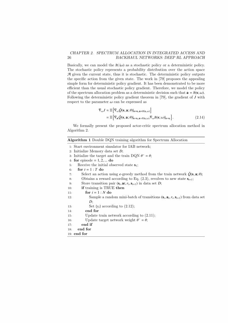
26CHAPTER 2. SPECTRUM ALLOCATION IN INTEGRATED ACCESS AND
BACKHAUL NETWORKS: DEEP RL APPROACH
Basically, we can model the π(·|ω) as a stochastic policy or a deterministic policy.The stochastic policy represents a probability distribution over the action spaceA given the current state, thus it is stochastic. The deterministic policy outputsthe specific action from the given state. The work in [79] proposes the appealingsimple form for deterministic policy gradient. It has been demonstrated to be moreefficient than the usual stochastic policy gradient. Therefore, we model the policyof the spectrum allocation problem as a deterministic decision such that a = π(s;ω).Following the deterministic policy gradient theorem in [79], the gradient of J withrespect to the parameter ω can be expressed as
∇ωJ ≈ E[∇ωQ(s, a; θ)|s=st ,a=π(st ,ω)
]= E[∇a Q(s, a; θ)|s=st ,a=π(st ;ω)∇ωπ(s;ω)|s=st
]. (2.14)
We formally present the proposed actor-critic spectrum allocation method inAlgorithm 2.
Algorithm 1 Double DQN training algorithm for Spectrum Allocation
1: Start environment simulator for IAB network;2: Initialize Memory data set D;3: Initialize the target and the train DQN θ− = θ;4: for episode = 1, 2, ... do5: Receive the initial observed state s1;6: for t = 1 : T do7: Select an action using ε-greedy method from the train network Q(s, a; θ);8: Obtains a reward according to Eq. (2.3), revolves to new state st+1;9: Store transition pair (st, at, rt, st+1) in data set D;
10: if training is TRUE then11: for i = 1 : N do12: Sample a random mini-batch of transitions (si, ai, ri, si+1) from data set
D;13: Set yi according to (2.12);14: end for15: Update train network according to (2.11);16: Update target network weight θ− = θ;17: end if18: end for19: end for

2.2. SPECTRUM ALLOCATION WITH DRL 27
Algorithm 2 Actor-Critic Spectrum Allocation Algorithm(ACSA)
1: Start environment simulator for IAB network;2: Initialize Memory data set D;3: Initialize target critic and actor network, θ− = θ, ω− = ω;4: for episode = 1, 2, ... do5: Observed the initial state s1;6: for t = 1 : T do7: Select action at from actor network;8: Execute action at to the spectrum allocation matrix X and Z and obtains
reward rt;9: Store transition pair (st, at, rt, st+1) in data set D;
10: if training is TRUE then11: for i = 1 : N do12: Sample mini-batch from data set D;13: Set yi = ri + γQ(s′i , π(s′i ;ω
−); θ−);14: Compute TD error δi = yi − Q(si, ai; θ)15: end for16: Update θ for critic network according to (2.11);17: Compute sampled policy gradient
∇ωJ ≈1N
∑i
∇a Q(s, a; θ)|s=si,a=π(si;ω)
× ∇ωπ(s;ω)|s=si ;
18: Update ω for actor network by
ω =ω + β∇ωJ;
19: end if20: Update the weights of the target networks
θ− =τθ + (1 − τ)θ−;ω− =τω + (1 − τ)ω−;
21: end for22: end for
2.2.3 Numerical results
In this section, we provide numerical experiments of proportional fairness spectrumallocation in different IAB using the proposed algorithms.
We consider an IAB network consisting of one DBS at the center, and L IABnodes following the Poisson point process (PPP) deployed at the radius of 250-meter

28CHAPTER 2. SPECTRUM ALLOCATION IN INTEGRATED ACCESS AND
BACKHAUL NETWORKS: DEEP RL APPROACH
from DBS. UE groups are located at the radius of 150-meter from its associatedBS, the initial locations of which follow PPP. We adopt random walk model forsimulating the mobility of UEs in the IAB networks. The moving speed of UE u j
at time t follows uniform distribution, i.e., ν j∼ U(0, 2) m/s, while the moving angelfollows ψ j∼ U(0, 2π). The distance-based path loss is characterized by the line-of-sight (LoS) model for urban environments at 2.4 Ghz, and is compliant with theLTE standard [80]. The simulator initializes an IAB network setup according tothe parameters shown in Table. 2.1. We consider the proportional fairness objectivewhich aims to maximize
∑j∈U log(C j). The required rate is the same among all UEs,
where Ω j = 5,∀ j ∈ U.
Table 2.1: Simulator SetupParameter Value
Carrier Frequency 2.4 GhzBandwidth W 20 MhzDBS Pathloss 34 + 40 log(d)IAB Pathloss 37 + 30 log(d)Subchannel Rayleigh Fading
Transmit power at DBS 43 dBmTransmit power at IAB 33 dBm
Self-interference −70dBSpectral Noise −174dBm/Hz + 10 log(W) + 10dB
As shown in Fig. 2.1a, we compare the sum log-rate for the proposed DDQNand ACSA algorithms with the full-spectrum reuse strategy. The results show thatboth proposed methods can effectively learn from interacting with the time-varyingenvironment and achieve better sum log-rate performance than the full-spectrumreuse strategy. Fig. 2.1b illustrates one instance of the average rate of individualUE using ACSA method. It can be seen that the rates of UE1, UE2 and UE3increase rapidly after 100 steps. After around 300 steps, all UEs have achieved theirsystem requirement. To better understand the learning process of DRL methods,we show how allocation decisions are made in 4 consecutive time steps in one testrealization. The result is presented in Fig. 2.1d. It can be seen that the 6-thsub-channel is allocated for UE0 associated with MBS at the first 3 time steps.However, at the last time-step, the 3-rd sub-channel is allocated to UE0 insteadof sub-channel 6. For all the 4 steps, UE0 experiences cross-tier interference fromother two transmitting IAB nodes. As numerical result shown at this test case, asUE0 moves dynamically in the environment, the channel gain between UE0 andinterfering IAB nodes gi,u0 , i ∈ B
− varies. From step 3 to step 4, the interferenceintroduces by IAB node1 and node3 decreases while by which IAB node2 and node4increases.
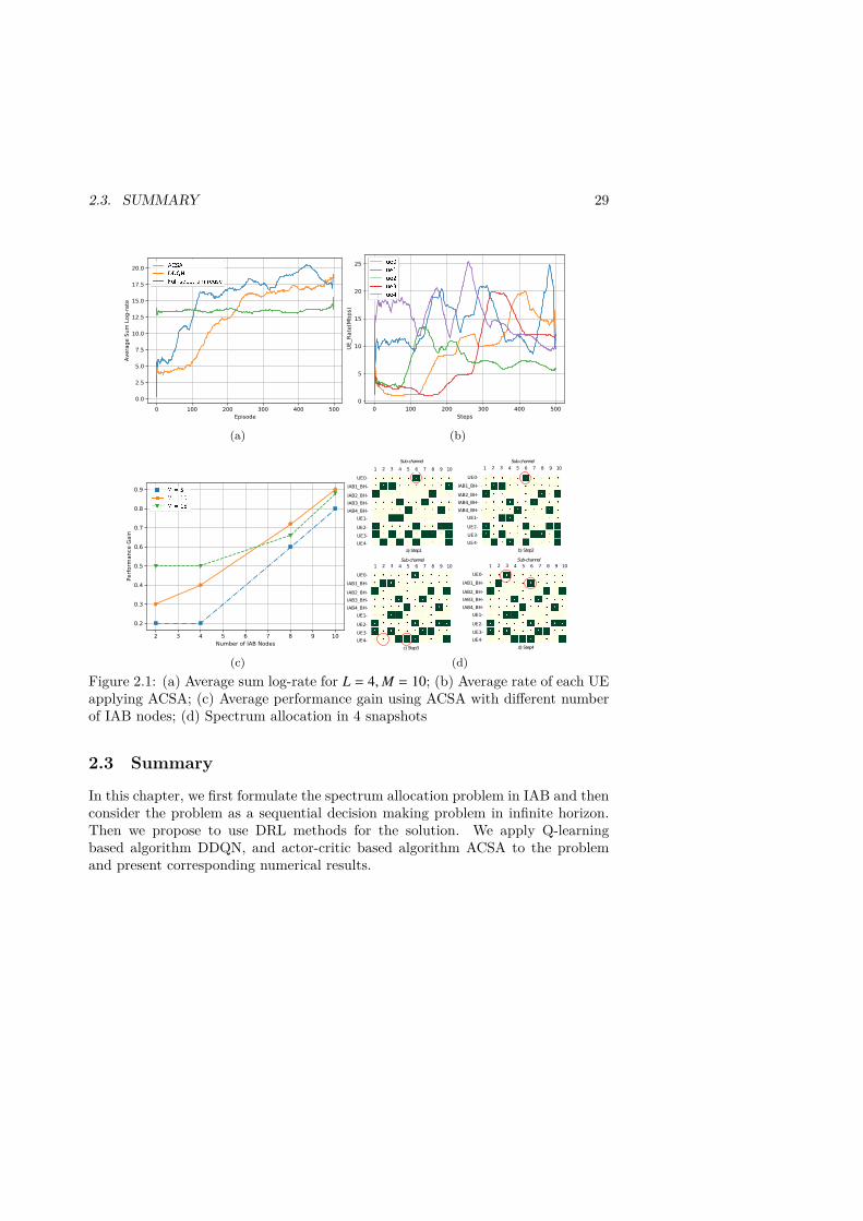
2.3. SUMMARY 29
0 100 200 300 400 500
Episode
0.0
2.5
5.0
7.5
10.0
12.5
15.0
17.5
20.0
Avera
ge S
um
Log-r
ate
(a)
0 100 200 300 400 500
Steps
0
5
10
15
20
25
UE_Rate(M
bps)
(b)
2 3 4 5 6 7 8 9 10
Number of IAB Nodes
0.2
0.3
0.4
0.5
0.6
0.7
0.8
0.9
Perf
orm
ance G
ain
(c)
Sub-channel
a) Step1 b) Step2
c) Step3 d) Step4
1 2 3 4 5 6 7 8 9 10 1 2 3 4 5 6 7 8 9 10
Sub-channel
1 2 3 4 5 6 7 8 9 10 1 2 3 4 5 6 7 8 9 10
Sub-channel Sub-channel
IAB2_BH-
IAB3_BH-
IAB4_BH-
UE1-
UE2-
UE3-
UE0-
IAB1_BH-
UE4-
IAB2_BH-
IAB4_BH-
IAB4_BH-
UE1-
UE2-
UE3-
UE0-
IAB1_BH-
UE4-
IAB2_BH-
IAB3_BH-
IAB4_BH-
UE1-
UE2-
UE3-
UE0-
IAB1_BH-
UE4-
IAB2_BH-
IAB3_BH-
IAB4_BH-
UE1-
UE2-
UE3-
UE0-
IAB1_BH-
UE4-
(d)Figure 2.1: (a) Average sum log-rate for L = 4,M = 10; (b) Average rate of each UEapplying ACSA; (c) Average performance gain using ACSA with different numberof IAB nodes; (d) Spectrum allocation in 4 snapshots
2.3 Summary
In this chapter, we first formulate the spectrum allocation problem in IAB and thenconsider the problem as a sequential decision making problem in infinite horizon.Then we propose to use DRL methods for the solution. We apply Q-learningbased algorithm DDQN, and actor-critic based algorithm ACSA to the problemand present corresponding numerical results.


Chapter 3
Decentralized RL in edge IoT:approximation in policy space
In this chapter, we study the policy gradient (PG) based RL in a decentralizedscenarios. PG methods focus on finding optimized parameters for a given policyparameterization. For RL in a decentralized setup, agents are connected through acommunication network aiming to work collaboratively to find a policy to optimizethe global reward as the sum of local rewards. The update of each agent’s pol-icy always suffers from high communication cost, scalability and adaptation issuesin complex environments. We apply ADMM approach and propose an adaptivestochastic Incremental ADMM (asI-ADMM) algorithm to the decentralized RLsettings.
This chapter is organized as follows: the decentralized RL with policy gradientmethod is presented in Section 3.1, and Section 3.2 introduces asI-ADMM algorithmfor decentralized RL and theoretical analysis for the algorithm. All the main resultsof this chapter are summarized in Section 3.3.
3.1 Decentralized RL
This section summarizes the formulated problem in decentralized RL and theADMM-based algorithm for solution. More details of this work are provided inPaper 1.
3.1.1 Decentralized RL problem formulation
Consider N agents located in a time-invariant communication network denoted byG:= (N ,E). A networked multi-agent MDP is characterized by tuple (S,A,P, β, α, gi∈N ),where S is the environmental state space and A is the action space; and P :S × A × S → [0, 1] is the state transition probability of the MDP; and α ∈ (0, 1)and β are the discounting factor and the initial state distribution, respectively; and
31
32CHAPTER 3. DECENTRALIZED RL IN EDGE IOT: APPROXIMATION IN
POLICY SPACE
gi: S ×A → R is the local loss function of agent i. The stochastic policy π : S → Amaps the state to a distribution of all possible actions given the current state st.
Two decentralized multi-agent MDP settings are considered: parallel agentsand collaborative agents. The former considers the scenario where agent i aimsto solve an independent MDP (Si,Ai,Pi, βi, α, gi∈N ), in which the local action andstate spaces as well as the transition probability of every agents are the same, i.e.,Si = S,Ai = A and Pi = P,∀i ∈ N . While in collaborative setting, all agents sharea global state st ∈ S, and at = (a1,t, a2,t, ..., aN,t) is a joint action and its space canbe denoted as A =
∏i∈N Ai, and at ∈ A. A main difference in collaborative setting
from parallel setting is that the joint action determines the transition probabilityto the next state st+1 as well as the local loss function gi(st, (a1,t, a2,t, ..., aN,t)).
In decentralized RL, the objective is to collaboratively find the consensus opti-mal policy π that minimizes the sum of discounted cumulative loss over all agents inthe network. With a policy π, we can generate an infinite horizon state-action tra-jectory ζi := s0, a0, s1, a1, ... with st ∈ S and at ∈ A. The problem can be expressedas following:
minπ
∑i∈N
Ji(π), s.t. Ji(π) = Eζi∼P(·|π)
∞∑t=0
αtgi(st, at)
, (3.1)
where Ji(π) is the cumulative loss for agent i. The expectation in (3.1) takes overthe random trajectory ζ of agent i under policy π. The probability of generatingtrajectory ζi given policy π is expressed as
P(ζi|π) = P(s0)∞∏
t=0
π(at |st)P(st+1|st, at), (3.2)
where P(s0) is the probability of initial state being s0, it is chosen randomly withregard to different initial state distribution of agent i, and P(st+1|s, a) is the transitionprobability from state st to state st+1 by taking action at.
The stochastic optimization problem in (3.1) has very nice differentialabilityproperties that are lacking in the original deterministic form as in [8]. By param-eterizing the policy π with parameters θ ∈ Rm, we denote the policy as π(·|s; θ), orπ(θ) for simplicity. Accordingly, the problem in (3.1) can be rewritten as
minθ
∑i∈N
Ji(θ), s.t. Ji(θ) = Eζi∼P(·|θ)
∞∑t=0
αtgi(st, at)
, (3.3)
where Ji(θ) is the long-term discounted loss of the parametric policy π(θ), and P(·|θ)is the probability distribution of sample trajectories ζi under the policy π(θ).
3.1.2 Policy Gradient methodProblem in (3.3) is a typical optimization problem and can be solved by gradientascent. The method requires that π(θ) is differentiable with respect to θ. The

3.1. DECENTRALIZED RL 33
solution relies on a convenient gradient formula, known as the log-likelihood trickand involves the natural logarithm of the sampling distribution. Combine (3.2) and(3.3), the gradient of cumulative loss Ji(θ) of each agent can be calculated as
∇Ji(θ) = ∇Eζi∼P(·|θ)
∞∑t=0
αtgi(st, at)
= ∇
∑θ∈X
P(ζ |θ)∞∑
t=0
αtgi(st, at)
=∑θ∈X
P(ζ |θ)
∇P(ζ |θ)P(ζ |θ)
∞∑t=0
αtgi(st, at)
= Eζi∼P(·|θ)
∞∑t=0
∇[log π(at |st; θ)]αtgi(st, at)
.
(3.4)
The above result is named ”Policy Gradient Theorem” which lays the theoreticalfoundation for various policy gradient algorithms:
∇Ji(θ) = Eζi∼P(·|θ)
∞∑t=0
∇[log π(at |st; θ)]αtgi(st, at)
. (3.5)
REINFORCE [81], also known as Monte-Carlo policy gradient, is usually adoptedto avoid costly full gradients computation (sometimes can be infeasible due toinfinite spaces) of ∇Ji(θ). Notably, Trust region policy optimization (TRPO) isproposed in [82], and it is similar to natural policy gradient method but is relativelycomplicate to implement. Then Proximal Policy Optimization (PPO) algorithm isproposed afterwards in [83]. PPO is shown to have the stability and reliability ofTRPO methods but is much simpler to implement. In our algorithm design andperformance analysis, we will leverage the REINFORCE for the sake of simplicityand generality for theoretical analysis.
Denote ζi,m = (si,m0 , ai,m
0 , si,m1 , ai,m
1 , ..., ai,mT−1, s
i,mT ) as the m-th T -slot trajectories gen-
erated by policy π(·|θ) at agent i. Hereby, the unbiased estimator of ∇Ji(θ) with them-th generated trajectory is given as follows
∇mJi(θ; ζm) =T∑
t=0
∇ log π(a[i,m]t |s[i,m]
t ; θ)
T∑t=0
αtgi(s[i,m]
t , a[i,m]t) , (3.6)
and the corresponding mini-batch PG is given as
di(θ; ζi) =1M
M∑m=1
∇mJi(θ; ζi,m). (3.7)
34CHAPTER 3. DECENTRALIZED RL IN EDGE IOT: APPROXIMATION IN
POLICY SPACE
3.2 Decentralized RL with adaptive stochastic ADMM
To solve decentralized problem in (3.3), there are normally two methods, primaland dual. The former is also referred as gradient-based. Each node averages itsiterations from neighbors and descends along its local negative gradient. The lattersolves an equivalent constrained form of the original problem and usually employsADMM-based methods.
3.2.1 ADMM for decentralized problemConsider a general ML problem with multiple nodes in decentralized computing,it can be formulated in a form where all distributed agents seek to collaborativelysolve one optimization problem:
f (θ) = minθ
N∑i=1
fi(θ), (3.8)
where fi(θ) := Eζ∼Di fi(θ; ζ), Di is a distribution associated with local data (or asensor collecting local data online) at agent i, and ζ is data points sampled via Di.Variable θ is shared across all agents. By defining Θ = [θ1, ...,θN] ∈ RmN , where θi
is the parameter at the i-th agent, problem (3.8) can be rewritten as
minΘ,z
∑i∈N
fi(θi), s.t. 1 ⊗ z −Θ = 0, (3.9)
where z ∈ X, and 1 = [1, ..., 1] ∈ RN , and ⊗ is the Kronecker product. The augmentedLagrangian for problem (3.9) is
Lρ(Θ,λ, z) =∑i∈N
fi(θi) + 〈λ,1 ⊗ z −Θ〉 + ρ2‖1 ⊗ z −Θ‖2, (3.10)
where λ = [λ1, ..., λN] ∈ RmN is the dual variable, while ρ > 0 is a constant parameter.Following I-ADMM [84], with guaranteeing
∑i∈N (θ0
i −λ0
iρ
) = 0, the updates of Θ, λand z at the (k + 1)-th iteration are given by
θk+1i :=
arg min
θi
Lρ(θi,λk, zk), i = ik;
θki , i , ik;
(3.11a)
λk+1i :=
λki + ργ(zk − θk+1
i ), i = ik;
λki , i , ik;
(3.11b)
zk+1 := zk +1N
θk+1ik −
λk+1ik
ρ
− θkik −
λkik
ρ
. (3.11c)

3.2. DECENTRALIZED RL WITH ADAPTIVE STOCHASTIC ADMM 35
In the stochastic update of (3.11a), a size of M mini-batch samples ζki are drawn
from the distribution Di, i.e., ζki , ζ
ki,m
Mm=1. We adopt the stochastic first-order
approximation such that fi(θi) ≈ 〈Gi(θki ; ζk
i ),θi − θki 〉, where Gi(θk
i ; ζki ) is the mini-
batch stochastic gradient given by
Gi(θki ; ζk
i ) =1M
M∑m=1
∇ fi(θ; ζki,m). (3.12)
Gi(θki ; ζk
i ) can be calculated with sampling methods. However, other sources ofnoise from stochastic objectives can cause large deviation in the result [85]. Inspiredby the idea in [77], we propose to use the first-moment estimation of gradients as
µk+1 := ηkµk + (1 − ηk)Gik (θkik ; ζk
ik ). (3.13)
Here µk+1 is the weighted exponential moving average (EMA) estimation of the truegradient, and the hyper-parameter ηk ∈ [0, 1) is controlling the exponential decayrate of the moving averages. When ηk → 0, the algorithm will effectively eliminatethe moving memory [86]. To bound the variance of EMA, we propose to apply thefollowing adaptive rule for the selection of ηk as
ηk =
η, (η)2‖µk −Gik (θ
kik ; ζk
ik )‖2 ≤
ι2
M;√
ι2
M1
‖µk −Gik (θkik
; ζkik
)‖, otherwise,
(3.14)
where η ∈ [0, 1) and ι ∈ R are pre-determined hyper parameters. The update ofΘk+1 can be rewritten as
θk+1i :=
arg minθi
Lρ(θi,λk, zk), i = ik;
θki , i , ik,
(3.15a)
where the approximated Lagrangian function is give by
Lρ(θi,λk, zk) = 〈µk+1,θi − θk
i 〉
+ρ
2‖zk − θi +
λki
ρ
∥∥∥2 + τ2
∥∥∥θi − θki ‖
2.(3.16)
where τ is the stepsize.The proposed asI-ADMM solution for problem in (3.9) is presented in Algorithm
3.
36CHAPTER 3. DECENTRALIZED RL IN EDGE IOT: APPROXIMATION IN
POLICY SPACE
Algorithm 3 Adaptive stochastic I-ADMM (asI-ADMM)
1: initialize: θ0i = λ
0i = z0 = µ0 = 0, k = 0, η, ι|i ∈ N;
2: for k = 0, 1, ... do3: agent ik = k mod N + 1 do:4: receive token µk, zk;5: randomly select M samples ζk
ikaccording to Di, and compute stochastic gra-
dient Gik (θkik
; ζkik
) ;6: choose ηk according to (3.14);7: update µk+1 according to (3.13);8: update θk+1
ikby (3.16);
9: update λk+1ik
according to (3.11b);10: update zk+1 according to (3.11c);11: send µk+1 and token zk+1 to agent ik+1 = (k + 1) mod N + 1;12: end for
Part of the convergence analysis for asI-ADMM is provided as follows.
Lemma 1. Suppose sequence Θk,λk, zk |k = 1, ...,K is generated from Algorithm 3,and let τ > L+ρ−1
2 , ρ > 1 and γ > 4N, we have
1K
K∑k=0
(E‖θkik − θk−1
ik ‖2 + E‖zk − zk−1‖2) 6
V0 −V∗
Kκ+ι2 + σ2
Mκ, (3.17)
where κ = min(χ, ϕ) with χ = ρ−2L+2τ+12 −
2ργ
and ϕ = Nρ2 −
2Nρ2
γ.
Theorem 1. Suppose sequence Θk,λk, zk |k = 1, ...,K is generated from Algorithm3, following the conditions given in Lemma 1 and choosing constants K = O( 1
ε),
M = O( 1ε), we have
1K
K∑k=0
E[‖∇L(Θk,λk, zk)‖2
]6ε(V0 −V∗)
Kκ+ε(ι2 + σ2)
Mκ6 ε,
(3.18)
where ε = 5 + 5L2 + 5τ2 + 15ρ2 + 10ρ2N2.
It is worth noting that since there is only one agent is active at iteration inAlgorithm 3, the computational complexity is mainly determined by the iterations.
3.2.2 ADMM for decentralized RLOur goal in decentralized RL is to find an optimal consensus policy to minimize theoverall loss across the agents. Thus, (3.3) has the same form as the optimization
3.2. DECENTRALIZED RL WITH ADAPTIVE STOCHASTIC ADMM 37
problem in (3.9). We propose to plug-in the algorithm asI-ADMM and implementit in an online fashion due to that the training samples in RL are generated inreal-time by interacting with the environment. The essential part of the algorithmis to use the weighted EMA estimator for true PG:
µk+1 = ηkµk + (1 − ηk)di(θ; ζi), (3.19)
where di(θ; ζi) is obtained from (3.7). The use of µ has critical importance indecentralized RL. The reason is that within heterogeneous agents appear in theenvironment, initial state distribution and local loss can be varying across theagents. The weighted estimation µ not only consists of gradient information fromcurrent batch samples, but also has the information from past gradient. Sending µas a token can be helpful for consensus convergence. We provide the asI-ADMM fordecentralized RL in Algorithm (4). The convergence for Algorithm (4) requires thesmoothness of the objective function in (3.3). Given the assumptions that local lossand cumulative loss to be bounded, and the gradient of log π(a|s; θ) and its partialderivatives to be bounded, it is sufficient to guarantee the smoothness of (3.3) andfurther provide the convergence property for Algorithm (4) as following.
Algorithm 4 asI-ADMM for decentralized RL1: initialize: θ0
i = λ0i = z0 = µ0 = 0, k = 0, η, ι|i ∈ N
2: for k = 0, 1, ... do3: agent ik = k mod N + 1 do:4: collect M trajectories ζk
ikwith parameter θk
ik, compute mini-batch PG com-
ponent dik (θkik
; ζkik
) according to (3.7);5: receive tokens µk and zk;6: choose ηk according to (3.14);7: update µk+1 according to (3.19);8: update θk+1
ikaccording to (3.11a);
9: update λk+1ik
according to (3.11c);10: update zk+1 according to (3.11b);11: send token zk+1 and µk+1 to agent ik+1 = (k + 1) mod N + 1;12: end for
Corollary 1. The sequence Θk,λk, zk |k = 1, ...,K generated from Algorithm 4satisfies convergence property (3.18) but with different Lipschiz constants Li|i ∈ N.
3.2.3 Numerical results
Since one major contribution in this work is the proposed algorithm asI-ADMMin decentralized problem, we firstly present results in decentralized least squareregression and decentralized logistic regression problems. We compare the accuracy

38CHAPTER 3. DECENTRALIZED RL IN EDGE IOT: APPROXIMATION IN
POLICY SPACE
100 101 102 103 104
communication cost
10-5
10-4
10-3
10-2
10-1
100
acc
ura
cy
EXTRA
DADMM
DGD
COCA
W-ADMM
prox. I-ADMM
prox. sI-ADMM
asI-ADMM
(a)
100 101 102 103 104 105
communication cost
10-4
10-3
10-2
10-1
100
acc
ura
cy
EXTRA
DADMM
DGD
COCA
W-ADMM
prox. I-ADMM
prox. sI-ADMM
asI-ADMM
(b)Figure 3.1: T = 50, ω = 0.3, r = 0.1: (a) Decentralized least square regression; (b)Decentralized logistic regression
defined by (3.20) with state-of-the-art methods in [37,38,41,43]
accuracy = 1N
N∑i=1
‖θki − θ∗‖2
‖θ0i − θ∗‖2
, (3.20)
where θ∗ is the optimal solution of (3.9). We can see in Figure 3.1 that there isgap between I-ADMM where a full batch is used at each iteration and stochasticI-ADMM (sI-ADMM) methods where only a mini-batch is used for updating (withratio r = 0.1 in our case). Our proposed asI-ADMM converges faster than othermethods and it also converges to a better optimal solution than sI-ADMM by usingthe same amount of samples.
Next we study the performance of the proposed online asI-ADMM in decentral-ized RL with two experiments: /textittarget localization and resource management.For target localization, we first present the performance for the homogeneous (non-scaled reward) case in Fig. 3.2. The proposed asI-ADMM converges within thesame iterations as IGD [87] and DGD [37] methods, and achieves at a better localoptimum. This is because there exists a lower bound for accuracy when a fixedstep size is adopted in gradient-based methods. Results for the heterogeneous case(scaled reward) are shown in Figure 3.3, and the superiority is more profound thanin homogeneous case. The individual reward of representative agents in Figure 3.3band Figure 3.3d (agents with a higher index have higher priority).
In computation resource management experiment, we modify the problem inmobile edge-cloud [88] to a decentralized parallel RL problem without a cloudserver. The total computation resource at agent i is denoted as Ci. Si = 0, 1, ...,Ci
is the state space to denote the available computation resources at time intervalt. The arrival rate of computation task Wi(t) follows a Poisson distribution withexpected value di. State transitions occur when a new task arrives, or when an oldtask finished. The action space is denoted as the number of request computation

3.3. SUMMARY 39
(a) (b)
0 100 200 300 400
Iteration
0
1
2
3
4
5
6
Co
nse
nsu
s E
rro
r
10-3
(c)
0 100 200 300 400
Iteration
0
2
4
6
8
Co
nse
nsu
s E
rro
r
10-3
(d)Figure 3.2: Iteration and communication complexity in homogeneous environment:(a)(c) N = 5, IGD (γ = 0.095), DGD (α = 0.09), asI-ADMM (ρ = 1, τ = 10, η = 0.8); (b)(d) N = 10, IGD (γ = 0.095), DGD (α = 0.09,), asI-ADMM (ρ = 1, τ = 10, η =0.8).
resource Ai = 0, 1, ...,Ci. The immediate reward is defined as
gi(t) =
−h0Iat>0 − h1st
− h2((st + at) ∧C − st)+
+ p((st + at) ∧C − st+1)+,if event triggers;
−h1st, otherwise,
(3.21)
where a ∧ b = min(a, b) and (a)+ = max(a, 0), and h0 is fixed costs for initiatinga request and h2 is the price for each resource, and h1 is the cost for holding theresource, and p is the price for finishing a task. The detailed results are presented inFig. 8 of Paper 2. The results show that the policy learned by asI-ADMM achievesan average of 2 profits compared with a random policy, which only achieves average0.
3.3 Summary
In this chapter, we first study the communication efficient ADMM-based algorithmsfor solving decentralized consensus problem. We provide theoretical analysis for

40CHAPTER 3. DECENTRALIZED RL IN EDGE IOT: APPROXIMATION IN
POLICY SPACE
(a) (b)
(c) (d)Figure 3.3: Iteration and communication complexity in heterogeneous environment(scaled reward and different initial state distribution): (a)(b) N = 5, IGD (γ =0.095), DGD (γ = 0.095), asI-ADMM (ρ = 1, τ = 10, η = 0.8) ; (c)(d) N = 10, IGD(γ = 0.01), DGD (γ = 0.01), asI-ADMM (ρ = 1, τ = 10, η = 0.8).
the algorithms and evaluate the performance in two decentralized RL settings.The results is demonstrated to be communication-efficient and adaptive in complexenvironments. Besides, it also shows that the proposed methods can achieve goodtrade-off between the communication load and running time.

Chapter 4
Joint beam tracking and datatransmission control in mmWave:rollout approach
In this chapter, we focus on the rollout method for decision making in joint beamtraining and data transmission for delay-sensitive communications in mmWave sys-tems. In the considered scenario, the sequential decision making problem is formu-lated as a constrained MDP which aims to maximize the cumulative energy con-sumption over the considered period of time. Observing that most existing policiesfor beam training in the open literature invoke beam training at each transmissionblock, this would cause large overhead and cause decrease the overall throughputin the network. We investigate the rollout-based RL method and parallel rolloutwhere multiple baseline policies are adopted in the computation. We further showthat the proposed data-driven algorithm provides a variance reduction nature.
This chapter is structured as follows. Section 4.1 presents the system problemformulation for joint beam training and data transmission control, based on whichthe rollout-based data driven method is described in Section 4.2. Then the mainpoints are summarized in Section 4.3.
4.1 Beam training and data transmission in mmWavecommunications
This section summarizes the model and control problem in beam training and datatransmission for delay-sensitive mmWave communications. More details of problemformulation are presented in Paper 3.
41
42CHAPTER 4. JOINT BEAM TRACKING AND DATA TRANSMISSION
CONTROL IN MMWAVE: ROLLOUT APPROACH
4.1.1 System modelIn this work, we consider a multiple-input single-output (MISO) system, in whicha transmitter (e.g., base station, BS) with Nt antennas is assumed to communicatewith a single antenna receiver (e.g., user equipment, UE). We adopt a ray-tracingmodel with L domain propagation paths given as
h =√
Nt
L∑i=1
ρiv(θi), (4.1)
where ρi and θi respectively denote the complex gain coefficient and normalizedAoD of the i-th path, and v(θi) is the array response vector with respect to θi
with i = 1, ..., L. In order to align with the scenarios for existing configurationsin practical problems, we assume that the N beams are taken from a predefinedcodebook, given by
V = [v(θ1), · · · , v(θN)]T , (4.2)where θn =
2π(n−1)N , ∀n = 1, ...,N. To determine the best beam, the transmitter
employs each of N beams sequentially to send a set of pilot symbols for beamtraining purpose. The received signal at the receiver can be expressed as
yn = hHfnsn + zn, (4.3)
where sn =√
P with P denoting the power per pilot transmission, and zn ∼ CN(0, ζ2)is the additive white Gaussian noise. The best beam n? is selected according to thebelow criteria
n? = arg max1≤n≤N
|y1|2, · · · , |yN |
2. (4.4)
Due to the movement of UE, its channel towards the BS changes constantly,leading to a time-varying RSRP in each beam. Specifically, when UEs move indifferent velocities, their corresponding beam coherence times (the period of timeduring which the serving beam is unchanged) are also different. Some UEs withslow moving speed may employ a serving beam for a long period while other fastermoving speed UEs only remain in a beam for very short periods. Therefore, it isdesired to tailor different beam training strategies in order to avoid unnecessarytraining overhead.
In this work, it is assumed that the channel within one transmission block re-mains constant but varies from one transmission block to another. The decision ofwhether or not to execute beam training and selection of an appropriate power levelfor data transmission are both determined at the beginning of each transmissionblock. In order to reduce the unnecessary training overhead and leave more timefor data transmission, the beam training may not be invoked in every transmissionblock. In addition to determining whether or not to execute beam training in thenext transmission block, the BS also needs to select an appropriate data transmis-sion power level for the next transmission block aiming to minimize the total energyconsumption in the whole transmission frame.

4.1. BEAM TRAINING AND DATA TRANSMISSION IN MMWAVECOMMUNICATIONS 43
4.1.1.1 Problem formulation
The control over beam training and data transmission is UE-specific. At each timek, the UE firstly feeds the current RSRP, rk ∈ 1, 2, ...,R , R, back to the BS. Withrk, nk, i.e., the index of the current serving beam, and some historical informationas detailed described below, the BS then makes a decision uk ∈ sweep, wait , Uabout whether or not to execute beam training at this time step. As for beamtraining stage, we can not observe the RSRP measurements of all N beams unlessa beam sweeping is performed, thus the information is incomplete. The historicalrecord is expressed as
Ik = ((n0, r0), (n1, r1), ..., (nk, rk), u0, ..., uk−1, k). (4.5)
However, when the considered time horizon is infinite, the size of Ik increases with-out bound. By observing that the records before the latest beam sweeping becomeless relevant to the current and future decision, we employ a partial historical recorddefined as
Ik = ((nk1 , rk1 ), (nk1+1, rk1+1), ..., (nk, rk), tk), (4.6)
where tk is the number of time steps from k1 to k − 1, and thus tk = k − k1. To thisend, the evolution of nk, rk and tk in Ik can be given by
nk+1 =
arg max
1≤i≤N|yk,i|
2, uk = sweep,
nk, uk = wait,(4.7)
rk+1 =
max1≤i≤N
|yk,i|2, uk = sweep,
|yk,nk |2, uk = wait,
(4.8)
tk+1 =
0, uk = sweep,tk + 1, uk = wait.
(4.9)
Besides, we assume that the total number of symbol durations in one transmissionblock is denoted as Z, each sweep decision consumes τZ durations with τ ∈ [0, 1]and a constant of % energy. Meanwhile, the wait decision does not consume pilotoverhead or energy.
In addition, the BS will select an appropriate transmission power mk ∈ 0, 1, ..., M ,M for data transmission. The transmission buffer is assumed to be a first-in first-out queue. The delay-sensitive application can inject l packets into transmissionbuffer in each time step. The arriving packets are stored in a finite-length bufferwith size B. Thus the evolution of buffer state, bk ∈ B = 0, 1, ..., B, is given by
b0 = binit, (4.10)bk+1 = min(bk − ψ(Ik, uk,mk) + lk, B), (4.11)

44CHAPTER 4. JOINT BEAM TRACKING AND DATA TRANSMISSION
CONTROL IN MMWAVE: ROLLOUT APPROACH
where b0 is the initial buffer state, and ψ(Ik, uk,mk) is the transmission rate at timestep k. Here ψk is a random variable and can be derived as
ψ(Ik, uk,mk) =max(bk,Z(1 − τIsweep(uk)) log2(1 + SNRk)),
(4.12)
where SNRk is obtained after the beam training and power level decision.To this end, we introduce two cost functions, the energy cost g(·) and the buffer
cost c(·) as following:
g(Ik, uk,mk) =
% + m2k(1 − τ)Z, uk = sweep,
m2kZ, uk = wait.
(4.13)
c(bk, Ik, uk,mk) = Elk ,ψk (bk − ψk)︸ ︷︷ ︸holding cost
+ ξmax(bk − ψk + lk − B, 0)︸ ︷︷ ︸overflow cost
, (4.14)
Let π : X → A denote a stationary policy mapping states to actions such thata = π(x),∀x ∈ X. The objective for the delay-sensitive networks in mmWave systemis to minimize the infinite horizon expected energy cost subject to a constraint onthe infinite horizon expected transmission delay. Mathematically, it is expressed asbelow
minimize Gπ(x); s.t. Cπ(x) ≤ σ, ∀x ∈ X, (4.15)where σ is the transmission time delay constraint and
Gπ(x) = limK→∞E
K−1∑k=0
αkg(xk, π(xk), xk+1)|x0 = x, π, (4.16)
Cπ(x) = limK→∞E
K−1∑k=0
αkc(xk, π(xk), xk+1)|x0 = x, π. (4.17)
The problem in (4.15) is a constrained MDP problem and it can be reformulatedas an unconstrained one by introducing Lagrange multiplier associated with thedelay constraint. Firstly, we define a Lagrangian immediate cost function
jλ(x, a, x′) = g(x, a, x′) + λc(x, a, x′), ∀x ∈ X, a ∈ A(x), (4.18)
where λ ≥ 0 is the Lagrange multiplier. According to Thereom 1 provided inPaper 3, a policy π∗ is optimal for the constrained MDP if and only if
Lλ(x) = supλ≥0
Jλπ∗ (x) − λσ, (4.19)
whereJλπ (x) = Gπ(x) + λCπ(x)
= limK→∞E
K−1∑k=0
αk jλ(xk, π(xk), xk+1)|x0 = x, π.(4.20)

4.1. BEAM TRAINING AND DATA TRANSMISSION IN MMWAVECOMMUNICATIONS 45
Thus, solving the minimization of (4.15) is equivalent to solving the following dy-namic programming equation
Jλ,∗(x) =
mina∈A(x)
[∑x′∈X
Pxx′ (a)( jλ(x, a, x′) + αJλ,∗(x′))], ∀x ∈ X, (4.21)
where Jλ,∗ : X → R is the optimal cost function for state x. Then the optimal policycan be obtained from the minimization
πλ,∗(x) ∈ arg mina∈A(x)
Jλ,∗(x), x ∈ X. (4.22)
More details of the derivation can be found in Paper 3.
4.1.2 Learning the policy by rolloutWe firstly present the pure form of rollout method for the reformulated problem in(4.21). Then we provide data-driven implementation and parallel rollout algorithmsfor the joint beam training and data transmission control problem.
4.1.2.1 Data-driven rollout method
In the joint beam tracking and data transmission control problem mentioned above,the transition probability is an unknown priori. Therefore, we adopt model-free RLmethod such that the computation of expected value in (4.21) is done by Monte-carlo simulation. The basic idea in rollout is to compute some approximation Jof the optimal function J∗, and use one-step lookahead to implement a subopti-mal policy π ∈ Π. Rollout is a one-time policy iteration (PI) method, and itskey idea is policy improvement where the agent starts with a suboptimal/heuris-tic policy and produces an improved policy by limited lookahead minimizationwith the use of heuristic at the end. At the state xk = x, rollout firstly gen-erates on-line the next states xk+1 = x′ corresponding to all a ∈ A(x), and usesthe baseline policy π to compute the sequence of states xk+1, xk+2, ..., xk+T and ac-tions π(xk+1), π(xk+2), ..., π(xk+T−1). The rollout algorithm then applies the actionak ∈ A(x) that minimizes over the cost expression:
ak ∈ arg mina∈A(x)
∑xk+1∈X
Pxx′ (a)[ j(x, a, x′) + αJπ(x′)], (4.23)
where Jπ(x′) = limN→∞ E∑T
k=0 αt j(xk+1, π(xk+1), xk+2)|x1 = x′ is the cost function for
baseline policy π starting from state x′. An important character of rollout is thatit improves over the baseline policy. This is shown in Proposition 1 in Paper 3.
To compute the rollout action, a straightforward way is to generate a large num-ber of trajectories for each possible action at the current state. An ideal approach

46CHAPTER 4. JOINT BEAM TRACKING AND DATA TRANSMISSION
CONTROL IN MMWAVE: ROLLOUT APPROACH
to build such simulator is to learn a model of the system dynamic through regres-sion using collected state-action-next state samples. Another simpler approach isto conduct a search from the collected historical trajectories for a given state, andthen uses index to mark the trajectory for computation. We employ the second ap-proach and leave the first approach as our future work. The details of Data-drivenrollout computation is presented in Algorithm 5.
The collected dataset is denoted as D = T s : s = 1, ...,Ns which has Ns trajec-tories. The s-th collected trajectory is denoted as T s = (ys
i , rsi , n
si ) : i = 0, ..., |T s|−1,
where ysi ∈ R
N is the RSRP measurements for all beams at i-th step in s-th tra-jectory, and rs
i is the largest value among ysi with the corresponding optimal beam
index nsi , |T
s| is the length of trajectory T s.It is worth noting that the use of sampling in simulation for rollout or general
model-free RL methods is often organized to effect variance reduction. Different ac-tions of long trajectory simulation can lead to large variance in the result. We showthat data-driven approach using collected trajectory dataset with rollout providesa variance reduction nature. Denote the sample sequence as
ZT (x, a) = j(x, a, x1) + αtT−1∑t=1
j(xt, π(xt), xt+1), (4.27)
and we see that the approximation is based on the difference ZT (x, a) − ZT (x, a),which involves a common tail trajectory T for a and a. We then define the sampleerror (SE) as
S ET (x, a) = ZT (x, a) − Q(x, a), (4.28)
and we show in Proposition 1 that
Proposition 1. Given the above definition and assumption, we show the followinginequality holds
E[|S ET (x, a)−S ET (x, a)|2]
≥ E[|S ET (x, a) − S ET (x, a)|2].(4.29)
This shows that changes in the value of action a ∈ A(x) have little effect onthe value of error S ET (x, a) relative to the effect induced by the randomness of thetrajectory T .
4.1.2.2 Parallel rollout
For the problem at hand, there exists several baseline policies, e.g., exhaustivesweeping with random or fixed power level, greedy sweeping with random or fixedpower level, etc. It is then possible to use all of these base policies in the rolloutframework. Assume that we have M baseline policies and denoted them as π1, ..., πM,then the approximated cost function is expressed as
J(x) = minJπ1 (x), ..., JπM (x), ∀x ∈ X, (4.30)

4.1. BEAM TRAINING AND DATA TRANSMISSION IN MMWAVECOMMUNICATIONS 47
Algorithm 5 Data-driven RolloutData: D, current state x, baseline policy πResult: rollout control π(x)1. Initialize: At time k = 0, initialize the state x0 = (I0, b0), λ = λ02. At time k = 0, 1, ..., observe the state xk = (Ik, bk)3. Locate the trajectory indexes set Ixk = (i, s)l : l = 1, ...,Nm in D such that
nsi = n0, rs
i = r0 and rsi+ j = r j,∀0 < j < k. for a = [u,m] ∈ A(xk) do
4. Initialize the l-th Q-factor for the state-action pair (xk, a) as Ql(xk, a) = 05. Observe (n1, r1) from found trajectory ys
i+1, compute b1 according to (4.11),obtain x1
6. Obtain immediate cost jλk (xk, a, x1) according to (4.18)7. Thereafter, initialize z = 1 and Jπ(x1) = 0, run the following simulation usingbaseline policy π
for z ≤ T do8. Repeat steps 5,6 using action π(xz)9. Compute the approximate value for Jπ(xz):
Jπ(x1) = Jπ(x1) + αz jλk (xz, π(xz+1), xz+1); (4.24)
10. Compute Q-factor sample as
Ql(xk, a) = jλk (xk, a, x1) + Jπ(x1); (4.25)
11. z = z + 1;end12. Average Nm Q-factor samples
Q(xk, a) =1
Nm
Nm∑l
Ql(xk, a); (4.26)
end13. Select action such at π(xk) ∈ mina∈A(xk) Q(xk, a)14. Update Lagrange multiplier according to λk+1 = max0, λk + γk[c(xk, ak, xk+1) −
(1 − α)σ]
where Jπm (x) is obtained similarly as Jπ in (4.23). We also show that the policyobtained from (4.30) improves over each of the given baseline policies in π1, ..., πM.
Proposition 2. Let π be the rollout policy obtained by using J as one-step lookaheadapproximation, where J is obtained from (4.30), and it improves over each of thepolicies π1, ..., πM, i.e.,
Jπ(x) ≤ J(x) = minJπ1 (x), ..., JπM (x),∀x ∈ X. (4.31)

48CHAPTER 4. JOINT BEAM TRACKING AND DATA TRANSMISSION
CONTROL IN MMWAVE: ROLLOUT APPROACH
The implementation for parallel-rollout is described in Algorithm 6. More de-tails for the derivation of Proposition 2 and Algorithm 6 can be found in Paper3.
Algorithm 6 Data-driven Parallel RolloutData: D, current state x, baseline policies π1, ..., πM
Result: rollout control π(xk)Follows steps 1, 2, 3 as in Algorithm 5 for a = [u,m] ∈ A(xk) do
Run steps 4, 5, 6 as in Algorithm 5end8. For each baseline policy πm, run steps 7-8 to obtain Jπ1 (x1), ..., JπM (x1)9. Use J(x1) = Jπ1 (x1), ..., JπM (x1) to compute Q-factor sample:
Ql(xk, a) = jλk (xk, a, x1) + J(x1). (4.32)
Follow steps 10, 11 as in Algorithm 5.
4.1.3 Numerical resultsThe parameters used in the simulations are provided in Table. 4.1. The dataset iscollected from ray-tracing model in [89]. BS is placed on the right side of a crossing.There are two main roads that are covered by the BS, one vertical direction and onehorizontal direction. The length and width of each road is 120-meter and 18-meter,respectively. We use a discounted factor of α = 0.98 in the optimization objective in(4.15). The discount delay is converted to average delay constraint one, and we runthree different delay constraints, i.e., (1−α)σ = [1, 2, 3] corresponding with Poissonparameter lp = 2.
A typical result of fast-moving UE performance using parallel-rollout methodsis shown in Fig. 4.1. As Type-II UE is associated with fast beam variation, itmay require more frequent beam sweeping than slow-moving UEs and thus makeit even more sensitive to power level action at transmission phase. Although thegreedy policy has better performance in overhead, its overall performance is worsethan the proposed rollout-based policy. The reason is that the greedy policy doesnot consider the impact of current action to the future. This can be seen in theresults of overflow cost where greedy policy lags behind the other two policies inall occasions.
It is worth noting that the length of baseline policy in computing the approx-imated cost function in rollout plays a important role in the performance. Forexample, the greedy policy which is just a simple version of rollout, and it appliesone-step-lookahead with a fixed approximated cost function without consideringthe effect of future cost from the given action. As a result, its performance isusually worse than rollout based method. Theoretically, the longer the length inrollout calculation, the better the rollout policy obtains. However, the computationcomplexity increases exponentially when action space increases. Therefore, meth-
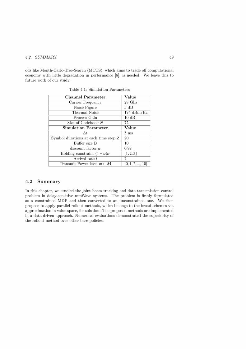
4.2. SUMMARY 49
ods like Month-Carlo-Tree-Search (MCTS), which aims to trade off computationaleconomy with little degradation in performance [8], is needed. We leave this tofuture work of our study.
Table 4.1: Simulation Parameters
Channel Parameter ValueCarrier Frequency 28 Ghz
Noise Figure 5 dBThermal Noise 174 dBm/HzProcess Gain 10 dB
Size of Codebook N 72Simulation Parameter Value
∆t 5 msSymbol durations at each time step Z 20
Buffer size B 10discount factor α 0.98
Holding constraint (1 − α)σ [1, 2, 3]Arrival rate l 2
Transmit Power level m ∈ M 0, 1, 2, ..., 10
4.2 Summary
In this chapter, we studied the joint beam tracking and data transmission controlproblem in delay-sensitive mmWave systems. The problem is firstly formulatedas a constrained MDP and then converted to an unconstrained one. We thenpropose to apply parallel-rollout methods, which belongs to the broad schemes viaapproximation in value space, for solution. The proposed methods are implementedin a data-driven approach. Numerical evaluations demonstrated the superiority ofthe rollout method over other base policies.

50CHAPTER 4. JOINT BEAM TRACKING AND DATA TRANSMISSION
CONTROL IN MMWAVE: ROLLOUT APPROACH
0 10 20
0.6
0.8
1Strict Constraint
0 1 20
0.5
1
0 10 20 300
0.5
1
0 100 2000
0.5
1
0 10 20
0.6
0.8
1Median Constraint
0 1 20
0.5
1
0 10 20 300
0.5
1
0 100 2000
0.5
1
0 10 20
0.6
0.8
1Relax Constraint
RL-rollout
exhaustive
greedy
0 1 20
0.5
1
0 10 20 300
0.5
1
0 100 2000
0.5
1
Figure 4.1: Performance of Type-II (fast-moving) UE, which shows probabilitydistributions of overflow, holding cost, overhead consumption and total cost on the1st, 2nd, 3rd and 4th row, respectively.
Chapter 5
Case study of beam tracking usingsupervised learning approach
In this chapter, we further study the problem of beam tracking with a supervisedlearning approach. We firstly introduce the adaptive beam tracking problem wherewe consider the beam tracking as a binary-classification problem. Then the typicalML processes including data preparation, data training and inference are presented.We test the proposed supervised learning methods on two scenarios: ray-tracingoutdoor scenario and over-the-air (OTA) real testing dataset from Ericsson. Weshow that the supervised learning approach in beam tracking provides low imple-mentation complexity and can improve cell capacity by reducing beam sweepingoverhead.
This chapter is structured as follows. Section 5.1 introduces the system overviewand methods. The experimental results in two scenarios are presented in Section5.2. Then the main points are summarized in Section 5.3.
5.1 System overview and methods
In this section, we present the problem formulation, based on which the data prepa-ration, ML training and inference process for solving the problems are provided.
5.1.1 Problem formulation for supervised learning
We formulate the beam tracking problem as a binary classification problem, withtwo classes (C1:sweep class and C0:wait class). At each decision time step, basestation receives the UE report denoted as x ∈ Rd regarding the serving beam andbeam sweep information, d is the dimensionality. We denote the true class labelof x as y ∈ 1, 0 of the received UE report. With enough amount of data, thetraining process using supervised learning takes place offline and outputs the trainedparameters, denote as w ∈ Rv, for future prediction. Here we use v instead of d,
51
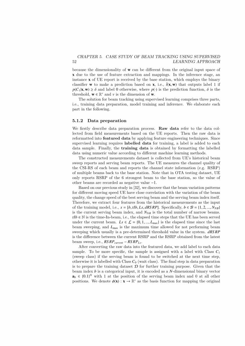
52CHAPTER 5. CASE STUDY OF BEAM TRACKING USING SUPERVISED
LEARNING APPROACH
because the dimensionality of w can be different from the original input space ofx due to the use of feature extraction and mappings. In the inference stage, aninstance x of UE report is received by the base station, which employs the binaryclassifier w to make a prediction based on x, i.e., t(x,w) that outputs label 1 ifp(C1|x,w) ≥ δ and label 0 otherwise, where p(·) is the prediction function, δ is thethreshold, w ∈ Rv and v is the dimension of w.
The solution for beam tracking using supervised learning comprises three parts,i.e., training data preparation, model training and inference. We elaborate eachpart in the following.
5.1.2 Data preparationWe firstly describe data preparation process. Raw data refer to the data col-lected from field measurements based on the UE reports. Then the raw data isreformatted into featured data by applying feature engineering techniques. Sincesupervised learning requires labelled data for training, a label is added to eachdata sample. Finally, the training data is obtained by formatting the labelleddata using numeric value according to different machine learning methods.
The constructed measurements dataset is collected from UE’s historical beamsweep reports and serving beam reports. The UE measures the channel quality ofthe CSI-RS of each beam and reports the channel state information (e.g. RSRP)of multiple beams back to the base station. Note that in OTA testing dataset, UEonly reports RSRP of the 6 strongest beam to the base station, so the value ofother beams are recorded as negative value −1.
Based on our previous study in [32], we discover that the beam variation patternsfor different moving speed UE have close correlation with the variation of the beamquality, the change speed of the best serving beam and the serving beam index itself.Therefore, we extract four features from the historical measurements as the inputof the training model, i.e., x = [b, tIb, Ls, dRS RP]. Specifically, b ∈ B = 1, 2, ...,NNB
is the current serving beam index, and NNB is the total number of narrow beams.tIb ∈ N is the time-In-beam, i.e., the elapsed time steps that the UE has been servedunder the current beam. Ls ∈ L = 0, 1, ..., Lmax is the elapsed time since the lastbeam sweeping, and Lmax is the maximum time allowed for not performing beamsweeping which usually is a pre-determined threshold value in the system. dRS RPis the difference between the current RSRP and the RSRP obtained from the latestbeam sweep, i.e., RS RPcurrent − RS RPLs.
After converting the raw data into the featured data, we add label to each datasample. To be more specific, the sample is assigned with a label with Class C1(sweep class) if the serving beam is found to be switched at the next time step,otherwise it is labelled with Class C0 (wait class). The final step in data preparationis to prepare the training dataset D for further training purpose. Given that thebeam index b is a categorical input, it is encoded as a N-dimensional binary vectorab ∈ 0.1N with 1 at the position of the serving beam index and 0 at all otherpositions. We denote φ(x) : x → Rv as the basis function for mapping the original

5.1. SYSTEM OVERVIEW AND METHODS 53
input vector x to the feature space φ. The labels are set to 0, 1 for logistic regressionand random forest, and are set to −1, 1 for ridge regression. Finally, the trainingdata is denoted as D = (xs, ts) : s = 1, ...,Ns where Ns is the number of samples inthe dataset.
5.1.3 ML algorithms and inference
Next we introduce the model training of supervised learning algorithms and theinference stage using the trained models. The goal of the model training is to obtaina model which can predict the output class of a given input vector as accurate aspossible. The model can be represented by some parameters, e.g. linear regressionand ridge regression classifier, or by an ensemble of several decision trees, e.g.random forest. We apply two types of models, 1) Linear Model: linear regression,ridge regression; 2) Random forest. We give details for each method in the following.
5.1.3.1 Linear Method
We firstly consider linear methods for supervised learning, by which we mean thatthe decision surface are linear functions of the input φ(x) and hence are defined by(v − 1)-dimensional hyperplanes within the v-dimensional input space.
• Logistic Regression: We model the conditional distributions p(C1|x; w), thendefine a loss function f (w;D) according to different classification models.The likelihood function of the classification dataset is denoted as p(D|w) =∏Ns
s=1 ytss (1 − ys)1−ts , where ys = p(C1|φs) = σ(wTφs), and σ(·) is the sigmoid
function expressed as σ(x) = 1(1+e−x) . One can use iterative weighted least
squares (IRLS) algorithm for the solution. The goal of model training isto find the parameters of w, which maximize the likelihood of the trainingdataset D defined above. Minimizing the negative log of the likelihood func-tion is usually used to calculate w, which is equivalent to maximizing thelikelihood function. The loss function is defined as f (w;D) = − ln p(D|w) ∝−∑Ns
s=1[ts ln ys+(1− ts) ln (1 − ys)], then the minimization problem can be solvedby iterative weighted least squares (IRLS) [90] or quasi-Newton method [91]for solution.
• Ridge Regression: The loss function is to minimize f (w; D) = ‖Φw−t‖22+α‖w‖22,
where t = −1, 1 and Φ ∈ RNs×v whose n-th row is given by φTs . The complexity
parameter α ≥ 0 controls the amount of shrinkage: the larger the value of α,the greater the amount of shrinkage and thus the coefficients become morerobust to collinearity. Thus, the solution of w can be obtained directly forthe computation of w = (ΦTΦ + αI)−1ΦT t.

54CHAPTER 5. CASE STUDY OF BEAM TRACKING USING SUPERVISED
LEARNING APPROACH
5.1.3.2 Random Forest Method
The training algorithm of random forest applies two main techniques, bagging andthe Classification-And-Regression-Trees (CART)-split criterion [92,93]. The train-ing parameters may comprise ntrees,maxdepth,minsamples plit,minsamplelea f ,max f eatures, bootstrapsample,etc. Specifically, ntrees is the number of trees in the forest, maxdepth is the maxi-mum depth of the tree, minsamples plit is the minimum number of samples requiredto split in each internal node of the tree, minsamplelea f is the minimum numberof samples required to be at a leaf node of the tree, max f eatures is the number offeatures to consider when looking for the best split, bootstrapsample is the num-ber of samples drawn from dataset D to train each base predictor, i.e. each treefor classification. Each trained tree can be represented by a function denoted asgi(φ) and outputs the classification result, either as value 1 for sweep class or value0 for wait class. The conditional probability of a given input x is expressed asp(C1|x) = 1/M
∑m gi(φ), where M is the number of trees (i.e. ntrees).
5.1.3.3 Inference
The inference stage is a straightforward calculation after obtaining the trainedmodel. Basically, the inference process contains the following steps:
1) Receive a UE report x and map it to the feature space φ(x);
2) Compute the prediction value for the UE feature vector φ(x), i.e. p(C1|x) orp(C0|x), from the trained model.
– Linear Modeli) For logistic regression, p(C1|x) is obtained by calculating σ(wTφ(x));ii) For ridge regression, p(C1|x) is obtained by calculating wTφ(x).
– Random Foresti) For the random forest method, p(C1|x) is obtained by applying theinput x to each trained tree function gi(φ(x)) and then p(C1|x) is obtainedby calculating the average by 1/M
∑i gi(φ(x)) where M is the number of
trees in random forest (i.e. ntrees).
3) Given a threshold δ for classification, use p(C1|x) to make the classificationdecision such that classified as the sweep class if p(C1|x) > δ, and classified asthe wait class if p(C1|x; w) ≤ δ. For the logistic regression and random forestmethods, δ = 0.5. For the ridge regression method, δ = 0.
5.2 Performance Evaluation
We evaluate the proposed supervised learning methods on two dataset: 1) datasetgenerated by ray-tracing model; 2) Over-The-Air (OTA) test data.

5.2. PERFORMANCE EVALUATION 55
Table 5.1: Ray-tracing parameters
Channel Parameter ValueCarrier Frequency (CF) 28 Ghz
Noise Figure (NF) 6 dBBandwidth (BW) 100 Mhz
Thermal Noise (TN) 174 dBm/HzGap 3 dB
Transmit power PT 23 dBm/antennaNumber of narrow beams Nnb 72
Beam steering angles [−60, 60] degreeNumber of subcarriers Nsc 792
In addition, we assume that each time step has C = 20 slots which can be usedfor tracking and transmission, the maximum allowed number of UE is Nue = 20.We denote the decision for i-th UE at k-th step as ti
k, the corresponding bitrateis denoted as rn
k = BW log2(1 + 10( SNRnk−Gap10 ), where BW is the bandwidth, Gap =
3 dB. The cell throughput at each step is obtained by calculating the value of∑Nuej=1[(C −
∑Nuei=1 ti
k)Nuer jk]/C.
5.2.0.1 Ray-tracing Model
A ray-tracing model are used to simulate the channel propagation in a simulatedarea, as shown in Figure 5.1. The length and width of the area is 120-meter and18-meter, respectively. We generate two types of UEs, one with random walk speed(0-3km/h) and one with west-driving speed ( 60km/h). Two types of UEs aregenerated, one with random walk speed (0-3km/h) and one with west-driving speed(60km/h). The simulation parameters is given in Table. 5.1. The base station isequipped with uniform linear array. Furthermore, the signal-to-noise radio (SNR)is calculated as SNR = RS RP(b) − PN , where PN = −TN + 10 log10(BW) + NF isbackground noise, and RS RP(b) = PT+10∗log10(Nnb)+10∗log10((
∑Nsci=1 |hi∗F(b)|2)/Nsc)
is the RSRP value of the current serving beam b. F(b) is the beamforming vectorcorresponding to beam b. The signal-to-noise radio (SNR) is calculated as S NR =RS RP(b) − PN , PN = −174 + 10 ∗ log10(BW) + NF is the background noise. RS RP(b)is the RSRP value of the current serving beam and it is expressed as RS RP(b) =23+10∗ log10(72)+10∗ log10((
∑792i=1 |hi ∗F(b)|2)/792), where F(b) is the beamforming
vector corresponding to the beam b.We present the results for average throughput, overhead consumption and RSRP
performance for the proposed supervised learning methods. As a reference, we alsopresent the existing periodic sweeping method, where UE performs beam sweepat a fixed period. Period k represents that UE performs one fully sweep every ksteps. For example, Period 3 performs beam sweep every 3 steps. And Period 1is equivalent to exhaustive sweep, which performs beam sweep at every step. As

56CHAPTER 5. CASE STUDY OF BEAM TRACKING USING SUPERVISED
LEARNING APPROACH
Figure 5.1: Ray-tracing model
shown in Fig.5.2, the average throughput for exhaustive sweeping decreases linearlywith the number of total UEs in the network, because more and more resources areused for beam sweeping at every time step. Regarding the RSRP performance inFig.5.2(a), supervised learning methods outperformed all periodic sweeps. It showsthat only 8% of the 20-UE tests with the logistic regression method lose morethan 1 dB RSRP than the optimal RSRP using exhaustive sweep. Regarding thethroughput performance in Fig.5.2(b), the logistic regression is superior than otherperiodical sweeping strategies. Regarding the overhead consumption Fig.5.2(c), itshows that all supervised learning methods result in different sweep overhead pertest since they adapt the beam sweep according to the UE reports. Regarding theRSRP performance shown in Fig.5.3(a), ML-based algorithms are slightly degraded
5.2.0.2 OTA testing data
The testing data is collected in Lund, Sweden by a combination of walk and bi-cyling speed. The coverage radius is a couple of hundred meters. The time elapsebetween two measurements are 40ms, UE only reported measurements of the moststrongest beams to the base station. Total number of narrow beams are 144. Thevalues for beams without measurements are reported as −1. The performance byproposed ML-based methods in OTA test data is similar as the one in ray-tracingmodel. Regarding the RSRP performance shown in Fig.5.3, Periodical sweepinghas better performance compared with the one in ray-tracing, specifically, Period3 outperforms other ML-based methods where only 10% of the 20-UE tests in Pe-riod 3 loss more than 1 dB RSRP, and only 15% in tests of Period 10 as shownin Fig.5.3a. The reason is that most of the UEs in OTA test data are with walk-ing speed, which means their beam variation can be relatively slower compared

5.3. SUMMARY 57
(a) (b)
(c) (d)Figure 5.2: Ray-tracing scenario, (a) RSRP performance distribution; (b) averagethroughput for different number of UEs; (c) OH consumption for supervised learn-ing with 20UEs; (d) OH consumption for periodical sweeping.
with fast moving UEs. However, logistic regression still achieves lowest overheadconsumption over the periodical sweeping strategies as shown in Fig.5.3c.
Overall, the experiments demonstrate that the proposed methods based on su-pervised learning can significantly improve the cell capacity by adaptively perform-ing beam sweeps per UE while they also keep high RSRP and low beam sweepoverhead simultaneously.
5.3 Summary
In this chapter, we present ML-based supervised learning method for the beamtracking problem at hand. We see that by using the proposed adative beam trackingscheme, the overhead consumed by CSI-RS can be reduced compared with theexisting periodic sweep method. Especially for a large number of connected UEs,the overhead consumption can be largely reduced by using the proposed adaptivesweeping decision. These symbols are released, for example, to carry data trafficinstead. It also means that more UEs can be served in a cell. Besides, the proposed

58CHAPTER 5. CASE STUDY OF BEAM TRACKING USING SUPERVISED
LEARNING APPROACH
(a) (b)
(c)Figure 5.3: OTA testing dataset, (a) RSRP performance distribution; (b) averagethroughput fo different number of UEs; (c) OH consumption for supervised learningwith 20UEs.
supervised learning approach is very light-weight and can be easily deployed in basestations.
Chapter 6
Conclusion and Future Work
To promote development of RL in wireless communications, it is crucial to model thedecision-making problem while selecting the proper approaches for implementation.To this end, deep RL approach is investigated for spectrum allocation problem inIAB networks. Approaches of policy gradient via approximation in policy spaceis studied in decentralized RL problem for edge IoT applications. Approaches ofrollout via approximation in value space is investigated in joint beam tracking anddata transmission control problem. A case study of beam tracking using supervisedlearning is further investigated as alternative approaches for comparison. All thekey findings and proposed solutions are summarized in the following section.
6.1 Concluding Remarks
6.1.1 Decision-making problems in wireless communications
The first contribution of this thesis is to model the sequential-decision-making prob-lem in wireless communications, and then to apply RL based methods for solution.
• RQ1: How to model decision-making problem in wireless communications toapply RL based methods?
By exploiting the characteristics of problems in different scenarios of wireless com-munications, we studied the method of modeling decision-making problem. To thisend, the spectrum allocation problem in IAB networks was first studied, where theoriginal static problem is non-convex mix integer and becomes intractable when thenetwork increases. We model the dynamic problem as an MDP, where the elementsin MDP are defined based on the system characteristics. The joint beam track-ing and data transmission control problem was further studied, which we modelthe problem as constrained MDP and convert it to unconstrained one. The mainfindings of this contribution are
59
60 CHAPTER 6. CONCLUSION AND FUTURE WORK
• Regarding the spectrum allocation problem in IAB networks (Paper 1), theobjective of which is to maximize a generic network utility function, the dy-namics is from the varying wireless channel of moving UEs.
• Regarding the joint beam tracking and data transmission control problem(Paper 3), the formulated constrained MDP aims to minimize the cumula-tive energy consumed over the whole considered period of time under delayconstraint in the presence of stochastic mmWave channel and packet arrivalrate. In order to avoid leveraging additional inaccessible information to thestate, meanwhile guaranteeing the markov property, we used partial historicalrecord which only contains RSRP related information. Instead of optimizingthe candidate beam set, we use binary decision for beam tracking and employdiscrete space for power selection to optimize the total energy consumption.
Besides, in the experiments of decentralized RL (Paper 2), we proposed the model-ing of homogeneous and heterogeneous environment to evaluate the performance ofthe proposed algorithms. It shows that the algorithms have different performancewith little changes in the original models.
6.1.2 RL algorithms: deep RL, decentralized RL with ADMMand rollout
The second contribution of this thesis is to design different RL algorithms concern-ing implementation feasibility, robustness and communication efficiency for prob-lems in wireless communications. This contribution answers the following researchquestions.
• RQ2: How to design efficient, robust RL algorithms for problems in wirelesscommunications? How to design decentralized RL scheme to achieve goodtrade-off between communication cost and convergence efficiency?
The deep RL algorithms for solving spectrum allocation problem in IAB is firststudied. The Q-learning and actor-critic structure enable the model-free methodsfor the solution and show to achieve improved performance. Due to that the IABnetworks are large-scale and complicated, the computational complexity of the RLtechniques becomes unmanageable quickly. As a result, deep RL has been developedto be an alternative to overcome the challenges. By developing the DDQN andACSA algorithms for the spectrum allocation, the spectrum allocation problemcan be solved in model-free manner. The main findings of this work are
• We develop a novel model-free framework based on DDQN and actor-critictechniques for dynamically allocating spectrum resource with system require-ments. The proposed architecture is simple for implementation and doesnot require CSI related information. The training process can be performedoff-line at a centralized controller, and the updating is required only whensignificant changes occur in IAB setup.

6.1. CONCLUDING REMARKS 61
• Regarding the performance, we show that with proposed learning framework,the improvement of the existing policy can be achieved with guarantee, whichyields a better sum log-rate performance. Regarding the learning speed of twoalgorithms, we show that actor-critic based learning applying policy gradientfor Q-value maximization is more effective in convergence speed than value-based DDQN when action-space is large.
The policy gradient based method from approximation in policy space is theninvestigated for decentralized applications in edge IoT. Based on the study of gen-eral ML decentralized optimization problems, we propose an adaptive incrementalalgorithm using ADMM approach for solution. By showing that the decentralizedRL with policy graidnet can be formulated as consensus problems, we extend theproposed algorithm for online implementation. We demonstrate that the onlineversion is suitable for parallel RL and collaborative RL in decentralized settings.The main findings of this work are
• Regarding the decentralized optimization problems, a new adaptive stochasticincremental ADMM (asI-ADMM) is proposed. The updating follows a pre-determined order, a weighted exponential moving average estimation of thetrue gradient is estimated and sent as a token at each iteration. In order tostabilize the convergence property, the first-order approximation is appliedfor stochastic objective.
• Regarding the convergence property of the proposed decentralized algorithm,we provide convergence analysis and prove that the asI-ADMM has O( 1
k ) +O( 1
M ) convergence rate, where k denotes the iteration number and M denotesthe mini-batch sample size. Based on some common assumptions in decen-tralized RL, the extended online version of the algorithm is shown to achieveO( 1
k ) + O( 1M ) by REINFORCE estimator.
• Two empirical experiments in edge IoT network setting are evaluated using theproposed algorithm. Regarding the performance, the proposed asI-ADMMoutperforms the benchmarks in terms of communication costs and is alsoadaptive in complex setups.
In addition to RL scheme via approximation in policy space, we also considerthe joint beam tracking and data transmission control problem using schemes viaapproximation in value space. The problem is a constrained MDP. Based on theformulation and the specific characteristics of the problem, we propose parallel-rollout methods for solution. The main findings of this work are
• We propose to use rollout-based method for solving the unconstrained MDPproblem. We show that rollout method can guarantee performance improve-ment for a given baseline policy. In order to enhance the resulting per-formance and computation efficiency, we further propose a parallel rollout

62 CHAPTER 6. CONCLUSION AND FUTURE WORK
method which adopts multiple baseline policies simultaneously for computa-tion.
• To effectively deploy the rollout algorithm and avoid leveraging additionalinformation such as UE position and speed for the policy design, a data-driven approach is considered for implementation. With the proposed data-driven method, we demonstrate that the optimized policy via parallel-rolloutsignificantly outperforms the baseline policies in both energy consumptionand delay performance.
In addition, we also provide analysis to show that the data-driven approachwith rollout method has a variance reduction nature when applying the collectedtrajectory dataset.
6.1.3 Beam tracking problem in mmWaveIn the study of beam tracking problem in mmWave systems, we aim to design ef-ficient and intelligent solution based on RL to achieve better performance in datatransmission and overhead reduction. Considering the requirements of implemen-tation feasibility and the robustness performance in real system, we also conduct afurther study in beam tracking using supervised learning approach as alternativesfor comparison. This addresses the following research question
• RQ3: How to efficiently apply RL and ML approach for beam tracking prob-lems in mmWave and how to evaluate the results in terms of feasibility andsystem performance?
To this end, we have provided two schemes, the rollout-based RL method and thesupervised learning based ML method, for solving the beam tracking problem. Thedifferent formulations are elaborated, the learning performance of the proposedscheme is evaluated. The RL method considers the joint beam tracking and datatransmission simultaneously but requires relatively more computation power for thelearning process. The ML method considers only beam tracking stage and treatsthe problem as binary classification task, and it is light for implementation andonline inference. The main findings of this work are
• With the data-driven rollout-based RL method in joint beam tracking anddata transmission control problem, the problem is firstly formulated as asequential-decision-making problem. Then we design the MDP structure withstate space, action space and reward function in order to make the currentstate to be separate the past from the future. The performance of using RLare evaluated in terms of overhead consumption, transmission delay and totalenergy consumption. The results demonstrate that the optimized policy viadata-driven parallel-rollout outperforms the exhaustive and greedy baselinepolicies.

6.2. DISCUSSIONS AND FUTURE WORK 63
• With the supervised learning method for beam tracking, the problem is for-mulated as a binary-classification task with two classes, sweep and wait. Theaim is to reduce the overhead caused by performing beam sweeping when thenumber of UE increases in the network and thus improve total cell capac-ity. Based on the investigations in beam tracking literature, we extract fourfeatures as input from field historical measurement of the UE reports. Andthen we label each data sample with one of the two classes. Three modelsare considered for training process. Finally the trained models are evaluatedin ray-tracing and over-the-air testing dataset. It shows that the proposedmethods can significantly improve cell capacity and reduce overhead especiallywhen the number of UEs increases in the network.
6.2 Discussions and Future Work
This thesis investigates the application of RL in wireless communications and pro-vides different RL based algorithms for solving decision-making problems. Althoughthe thesis covers many aspect, there are nevertheless some limitations and can beextended in several aspects. We discuss the limitations and potential extensions ofthis thesis work in the following subsections.
6.2.1 Decision-making problems in wireless communications
One of our contribution is to provide modeling methodology for decision-makingproblems in wireless communications in order to apply model-free RL algorithms.In this work, the problems are formulated as MDP by defining the system state,action, and reward function. For example, the work of spectrum allocation in IAB(Paper 1) uses the QoS indicator as the state and the allocation matrix as theaction, the immediate rate as the reward. However, this model has simplified thereal system because the immediate rate can not be obtained immediately after ac-tion execution. Besides, the dynamics of UE movement is hardly stationary overinfinite horizon, thus a more sophisticated scheme is needed to take into accountfor these issues. Regarding the state selection, the basic guideline is that the stateshould compass all the information and separate the past from the future, i.e., thestate has a markov property. The work of beam tracking and data transmission(Paper 3) uses historical record as the state due to the lack of complete channelinformation from all available beams at each time step. Such approach makes thestate space increases rapidly and becomes unmanageable. To provide guide for for-mulating decision-making problem in a manner that is suitable for RL algorithm,our future work to extend the thesis with concerning modeling can contain the fol-lowing aspects: (1) investigating the stationary and non-stationary characteristicsof MDP, (2) studying the design for reward function and delayed reward scenarios,(3) studying the characteristics of partial observed MDP and corresponding solu-tion. The main ideas of these aspects are to provide a basis guideline for problem

64 CHAPTER 6. CONCLUSION AND FUTURE WORK
formulation techniques, solution methods and adaptation of various RL algorithmsto various contexts in wireless communications. The challenges of this work are tofind out the underlying dynamics of the original decision-making problem and iden-tify the suitable states, actions as well as reward functions, and how to integrateRL based algorithms for solving the formulated decision-making problems.
6.2.2 RL algorithms with reliability and robustnessAnother contribution of this thesis is to show that RL has been developed as apromising and alternative solution for many problems in wireless communications.The advantages of applying RL includes followings. RL provides sophisticated so-lution for network optimization, as we show in (Paper 1) for using deep RL inspectrum allocation. RL-based framework allows network entities to learn consen-sus policy in decentralized settings (Paper 2) and provides autonomous decision-making. Most RL methods guarantee the improvement of baseline policies (heuris-tics) as shown in (Paper 1) and (Paper 3). However, the reliability and robustnesshave not been intensively studied or investigated regarding the deployment of RLalgorithms in real-world applications. Most of the existing RL algorithms eitherdepend heavily on the off-line computation from a pre-built simulator which is usedto represent the behavior and dynamics of the real system, or depend on the largeamount of samples that obtained from collected historical data such as DDQN andMAB related methods. Besides, the solutions provided in wireless communicationsusually have more rigorous requirements in reliability and robustness. By reliabilityit means that the solution should be performing constantly well without frequentfailure which is caused by the design of the solution. By robustness it means theRL algorithms need to be able to withstand the converse conditions and provideguaranteed performance with presence of disturbances. Therefore, following the re-search line on RL and its application in wireless communications presented in thisthesis, our future work is to extend the study of RL applications and investigatethe variants of RL algorithms in order to provide suitable and feasible solutions inthe context of wireless communications.
6.2.3 When should we use RL?Last discussion for this thesis is about when should we use RL (and when notto)? We see that since the success of RL in AlphaGo and AlphaZero, there isso much hype around RL nowadays. It is certainly a very important frameworkthat still has a lot of potentials. However, RL can not solve every decision-makingproblems (or not yet). Even though the deep RL embraces the advantages of DNNsto train the learning process, the lack of interpretability for such models makes itdifficult to be checked for consistency or cast the use of such representation tosafety-critical applications. One possible way to effectively apply RL in wirelesscommunication problems is to consider following questions before applying: (1) Howmuch the system can afford to make mistakes? (2) What state variable can be used

6.2. DISCUSSIONS AND FUTURE WORK 65
to represent the dynamics of the system? (3) Is the reward function designed clearand concrete for the objective? If we can not provide answers to these questionsin satisfactory way, we probably should look somewhere else for a way to deal withthe tasks at hand.


Bibliography
[1] D. Silver, A. Huang, C. J. Maddison, A. Guez, L. Sifre, G. Van Den Driessche,J. Schrittwieser, I. Antonoglou, V. Panneershelvam, M. Lanctot et al., “Mas-tering the game of go with deep neural networks and tree search,” nature, vol.529, no. 7587, p. 484, 2016.
[2] C. Berner, G. Brockman, B. Chan, V. Cheung, P. Dębiak, C. Dennison,D. Farhi, Q. Fischer, S. Hashme, C. Hesse et al., “Dota 2 with large scaledeep reinforcement learning,” arXiv preprint arXiv:1912.06680, 2019.
[3] G. Dulac-Arnold, D. Mankowitz, and T. Hester, “Challenges of real-worldreinforcement learning,” arXiv preprint arXiv:1904.12901, 2019.
[4] L. Matignon, G. J. Laurent, and N. L. Fort-Piat, “Reward function and initialvalues: Better choices for accelerated goal-directed reinforcement learning,” inInternational Conference on Artificial Neural Networks. Springer, 2006, pp.840–849.
[5] P. Xu, F. Gao, and Q. Gu, “Sample efficient policy gradient methods withrecursive variance reduction,” arXiv preprint arXiv:1909.08610, 2019.
[6] E. Greensmith, P. L. Bartlett, and J. Baxter, “Variance reduction techniquesfor gradient estimates in reinforcement learning.” Journal of Machine LearningResearch, vol. 5, no. 9, 2004.
[7] R. S. Sutton, A. G. Barto et al., Introduction to Reinforcement Learning. MITpress Cambridge, 1998, vol. 135.
[8] D. P. Bertsekas, Reinforcement Learning and Optimal Control. Athena Sci-entific, 2019.
[9] W. B. Powell, “A unified framework for stochastic optimization,” EuropeanJournal of Operational Research, vol. 275, no. 3, pp. 795–821, 2019.
[10] V. Chandrasekhar and J. G. Andrews, “Spectrum allocation in tiered cellu-lar networks,” IEEE Transactions on Communications, vol. 57, no. 10, pp.3059–3068, 2009.
67

68 BIBLIOGRAPHY
[11] B. Zhuang, D. Guo, E. Wei, and M. L. Honig, “Large-scale spectrum allocationfor cellular networks via sparse optimization,” IEEE Transactions on SignalProcessing, vol. 66, no. 20, pp. 5470–5483, 2018.
[12] Z. Zhou, X. Chen, Y. Zhang, and S. Mumtaz, “Blockchain-empowered securespectrum sharing for 5g heterogeneous networks,” IEEE Network, vol. 34, no. 1,pp. 24–31, 2020.
[13] Q. Yang, T. Jiang, N. C. Beaulieu, J. Wang, C. Jiang, S. Mumtaz, andZ. Zhou, “Heterogeneous semi-blind interference alignment in finite-snr net-works with fairness consideration,” IEEE Transactions on Wireless Commu-nications, 2020.
[14] C. J. Watkins and P. Dayan, “Q-learning,” Machine Learning, vol. 8, no. 3-4,pp. 279–292, 1992.
[15] D. P. Bertsekas, Dynamic programming and optimal control. Athena scientificBelmont, MA, 1995, vol. 1, no. 2.
[16] E. Ghadimi, F. D. Calabrese, G. Peters, and P. Soldati, “A reinforcementlearning approach to power control and rate adaptation in cellular networks,”in 2017 IEEE International Conference on Communications (ICC). IEEE,2017, pp. 1–7.
[17] Y. Zhang, C. Kang, T. Ma, Y. Teng, and D. Guo, “Power allocation in multi-cell networks using deep reinforcement learning,” in 2018 IEEE 88th VehicularTechnology Conference (VTC-Fall). IEEE, 2018, pp. 1–6.
[18] L. Zhang, J. Tan, Y.-C. Liang, G. Feng, and D. Niyato, “Deep reinforcementlearning-based modulation and coding scheme selection in cognitive heteroge-neous networks,” IEEE Transactions on Wireless Communications, vol. 18,no. 6, pp. 3281–3294, 2019.
[19] T. P. Lillicrap, J. J. Hunt, A. Pritzel, N. Heess, T. Erez, Y. Tassa, D. Silver,and D. Wierstra, “Continuous control with deep reinforcement learning,” arXivpreprint arXiv:1509.02971, 2015.
[20] G. Dulac-Arnold, R. Evans, H. van Hasselt, P. Sunehag, T. Lillicrap, J. Hunt,T. Mann, T. Weber, T. Degris, and B. Coppin, “Deep reinforcement learningin large discrete action spaces,” arXiv preprint arXiv:1512.07679, 2015.
[21] A. S. Leong, A. Ramaswamy, D. E. Quevedo, H. Karl, and L. Shi, “Deep rein-forcement learning for wireless sensor scheduling in cyber–physical systems,”Automatica, vol. 113, p. 108759, March 2020.
[22] C. She, R. Dong, Z. Gu, Z. Hou, Y. Li, W. Hardjawana, C. Yang, L. Song, andB. Vucetic, “Deep learning for ultra-reliable and low-latency communicationsin 6g networks,” IEEE Network, vol. 34, no. 5, pp. 219–225, July 2020.
BIBLIOGRAPHY 69
[23] Z. Lin, X. Li, V. K. Lau, Y. Gong, and K. Huang, “Deploying federated learningin large-scale cellular networks: Spatial convergence analysis,” arXiv preprintarXiv:2103.06056, July 2021.
[24] L. D. Nguyen, A. E. Kalor, I. Leyva-Mayorga, and P. Popovski, “Trusted wire-less monitoring based on distributed ledgers over nb-iot connectivity,” IEEECommunications Magazine, vol. 58, no. 6, pp. 77–83, July 2020.
[25] W. Liu, X. Zang, Y. Li, and B. Vucetic, “Over-the-air computation systems:Optimization, analysis and scaling laws,” IEEE Transactions on Wireless Com-munications, vol. 19, no. 8, pp. 5488–5502, May, 2020.
[26] P. Mach and Z. Becvar, “Mobile edge computing: A survey on architecture andcomputation offloading,” IEEE Communications Surveys & Tutorials, vol. 19,no. 3, pp. 1628–1656, March, 2017.
[27] J. Pan and J. McElhannon, “Future edge cloud and edge computing for internetof things applications,” IEEE Internet of Things Journal, vol. 5, no. 1, pp.439–449, Octorber, 2017.
[28] J. Baek, G. Kaddoum, S. Garg, K. Kaur, and V. Gravel, “Managing fog net-works using reinforcement learning based load balancing algorithm,” in IEEEWireless Communications and Networking Conference (WCNC), April 2019.
[29] W. Lei, Y. Ye, and M. Xiao, “Deep reinforcement learning-based spectrumallocation in integrated access and backhaul networks,” IEEE Transactions onCognitive Communications and Networking, vol. 6, no. 3, pp. 970–979, 2020.
[30] Y. Qian, R. Wang, J. Wu, B. Tan, and H. Ren, “Reinforcement learning-basedoptimal computing and caching in mobile edge network,” IEEE Journal onSelected Areas in Communications, vol. 38, no. 10, pp. 2343–2355, June 2020.
[31] M. Mohammadi, A. Al-Fuqaha, M. Guizani, and J.-S. Oh, “Semisuperviseddeep reinforcement learning in support of iot and smart city services,” IEEEInternet of Things Journal, vol. 5, no. 2, pp. 624–635, June, 2017.
[32] W. Lei, D. Zhang, Y. Ye, and C. Lu, “Joint beam training and data trans-mission control for mmwave delay-sensitive communications: A parallel re-inforcement learning approach,” IEEE Journal of Selected Topics in SignalProcessing, Jan 2022.
[33] X. Liu, J. Yu, Z. Feng, and Y. Gao, “Multi-agent reinforcement learning forresource allocation in iot networks with edge computing,” China Communica-tions, vol. 17, no. 9, pp. 220–236, June, 2020.
[34] S. Shalev-Shwartz, S. Shammah, and A. Shashua, “Safe, multi-agent, reinforce-ment learning for autonomous driving,” arXiv preprint arXiv:1610.03295, Oct,2016.

70 BIBLIOGRAPHY
[35] V. Mnih, A. P. Badia, M. Mirza, A. Graves, T. Lillicrap, T. Harley,D. Silver, and K. Kavukcuoglu, “Asynchronous methods for deepreinforcement learning,” in Proceedings of The 33rd International Conferenceon Machine Learning, ser. Proceedings of Machine Learning Research,M. F. Balcan and K. Q. Weinberger, Eds., vol. 48. New York, NewYork,: PMLR, 20–22 June 2016, pp. 1928–1937. [Online]. Available:http://proceedings.mlr.press/v48/mniha16.html
[36] A. Nedic and A. Ozdaglar, “Distributed subgradient methods for multi-agentoptimization,” IEEE Transactions on Automatic Control, vol. 54, no. 1, pp.48–61, January, 2009.
[37] K. Yuan, Q. Ling, and W. Yin, “On the convergence of decentralized gradientdescent,” SIAM Journal on Optimization, vol. 26, no. 3, pp. 1835–1854, June2016.
[38] W. Shi, Q. Ling, G. Wu, and W. Yin, “Extra: An exact first-order algorithmfor decentralized consensus optimization,” SIAM Journal on Optimization,vol. 25, no. 2, pp. 944–966, May, 2015.
[39] M. G. Rabbat and R. D. Nowak, “Quantized incremental algorithms for dis-tributed optimization,” IEEE Journal on Selected Areas in Communications,vol. 23, no. 4, pp. 798–808, April 2005.
[40] G. Qu and N. Li, “Accelerated distributed nesterov gradient descent,” IEEETransactions on Automatic Control, vol. 65, no. 6, pp. 2566–2581, August 2020.
[41] W. Shi, Q. Ling, K. Yuan, G. Wu, and W. Yin, “On the linear convergence ofthe ADMM in decentralized consensus optimization,” IEEE Transactions onSignal Processing, vol. 62, no. 7, pp. 1750–1761, April 2014.
[42] Y. Liu, W. Xu, G. Wu, Z. Tian, and Q. Ling, “Communication-censoredADMM for decentralized consensus optimization,” IEEE Transactions on Sig-nal Processing, vol. 67, no. 10, pp. 2565–2579, March, 2019.
[43] X. Mao, K. Yuan, Y. Hu, Y. Gu, A. H. Sayed, and W. Yin, “Walkman:A communication-efficient random-walk algorithm for decentralized optimiza-tion,” IEEE Transactions on Signal Processing, vol. 68, pp. 2513–2528, March2020.
[44] L. Busoniu, B. De Schutter, and R. Babuska, “Decentralized reinforcementlearning control of a robotic manipulator,” in 2006 9th International Confer-ence on Control, Automation, Robotics and Vision, 2006, pp. 1–6.
[45] A. Nair, P. Srinivasan, S. Blackwell, C. Alcicek, R. Fearon, A. De Maria,V. Panneershelvam, M. Suleyman, C. Beattie, S. Petersen et al., “Mas-sively parallel methods for deep reinforcement learning,” arXiv preprintarXiv:1507.04296, 2015.

BIBLIOGRAPHY 71
[46] K. Zhang, Z. Yang, H. Liu, T. Zhang, and T. Basar, “Fully decentralizedmulti-agent reinforcement learning with networked agents,” in InternationalConference on Machine Learning. PMLR, July, 2018, pp. 5872–5881.
[47] X. Zhao, P. Yi, and L. Li, “Distributed policy evaluation via inexact admm inmulti-agent reinforcement learning,” Control Theory and Technology, vol. 18,no. 4, pp. 362–378, November 2020.
[48] Z. Zheng, L. Song, Z. Han, G. Y. Li, and H. V. Poor, “Game theory for big dataprocessing: Multileader multifollower game-based admm,” IEEE Transactionson Signal Processing, vol. 66, no. 15, pp. 3933–3945, May 2018.
[49] T. Chen, K. Zhang, G. B. Giannakis, and T. Başar, “Communication-efficientdistributed reinforcement learning,” arXiv preprint arXiv:1812.03239, 2019.
[50] T. S. Rappaport, S. Sun, R. Mayzus, H. Zhao, Y. Azar, K. Wang, G. N.Wong, J. K. Schulz, M. Samimi, and F. Gutierrez, “Millimeter wave mobilecommunications for 5g cellular: It will work!” IEEE Access, vol. 1, pp. 335–349,2013.
[51] M. Xiao, S. Mumtaz, Y. Huang, L. Dai, Y. Li, M. Matthaiou, G. K. Kara-giannidis, E. Björnson, K. Yang, C. L. I, and A. Ghosh, “Millimeter wavecommunications for future mobile networks,” IEEE Journal on Selected Areasin Communications, vol. 35, no. 9, pp. 1909–1935, 2017.
[52] W. Roh, J. Y. Seol, J. Park, B. Lee, J. Lee, Y. Kim, J. Cho, K. Cheun, andF. Aryanfar, “Millimeter-wave beamforming as an enabling technology for 5gcellular communications: theoretical feasibility and prototype results,” IEEECommunications Magazine, vol. 52, no. 2, pp. 106–113, 2014.
[53] S. Hur, T. Kim, D. J. Love, J. V. Krogmeier, T. A. Thomas, and A. Ghosh,“Millimeter wave beamforming for wireless backhaul and access in smallcell networks,” IEEE Transactions on Communications, vol. 61, no. 10, pp.4391–4403, 2013.
[54] X. Li, J. Fang, H. Duan, Z. Chen, and H. Li, “Fast beam alignment formillimeter wave communications: A sparse encoding and phaseless decod-ing approach,” IEEE Transactions on Signal Processing, vol. 67, no. 17, pp.4402–4417, 2019.
[55] A. Alkhateeb, O. El Ayach, G. Leus, and R. W. Heath, “Channel estimationand hybrid precoding for millimeter wave cellular systems,” IEEE Journal ofSelected Topics in Signal Processing, vol. 8, no. 5, pp. 831–846, 2014.
[56] M. Kokshoorn, H. Chen, P. Wang, Y. Li, and B. Vucetic, “Millimeter wavemimo channel estimation using overlapped beam patterns and rate adapta-tion,” IEEE Transactions on Signal Processing, vol. 65, no. 3, pp. 601–616,2017.

72 BIBLIOGRAPHY
[57] S. Noh, M. D. Zoltowski, and D. J. Love, “Multi-resolution codebook andadaptive beamforming sequence design for millimeter wave beam alignment,”IEEE Transactions on Wireless Communications, vol. 16, no. 9, pp. 5689–5701,2017.
[58] Z. Xiao, T. He, P. Xia, and X.-G. Xia, “Hierarchical codebook design forbeamforming training in millimeter-wave communication,” IEEE Transactionson Wireless Communications, vol. 15, no. 5, pp. 3380–3392, 2016.
[59] V. Va, H. Vikalo, and R. W. Heath, “Beam tracking for mobile millimeterwave communication systems,” in IEEE Global Conference on Signal and In-formation Processing, 2016, pp. 743–747.
[60] S. Jayaprakasam, X. Ma, J. W. Choi, and S. Kim, “Robust beam-trackingfor mmwave mobile communications,” IEEE Communications Letters, vol. 21,no. 12, pp. 2654–2657, 2017.
[61] S. G. Larew and D. J. Love, “Adaptive beam tracking with the unscentedkalman filter for millimeter wave communication,” IEEE Signal ProcessingLetters, vol. 26, no. 11, pp. 1658–1662, 2019.
[62] J. Seo, Y. Sung, G. Lee, and D. Kim, “Training beam sequence design formillimeter-wave mimo systems: A pomdp framework,” IEEE Transactions onSignal Processing, vol. 64, no. 5, pp. 1228–1242, 2015.
[63] S. H. Lim, S. Kim, B. Shim, and J. W. Choi, “Efficient beam training andsparse channel estimation for millimeter wave communications under mobility,”IEEE Transactions on Communications, vol. 68, no. 10, pp. 6583–6596, 2020.
[64] D. Zhang, A. Li, M. Shirvanimoghaddam, P. Cheng, Y. Li, and B. Vucetic,“Codebook-based training beam sequence design for millimeter-wave trackingsystems,” IEEE Transactions on Wireless Communications, vol. 18, no. 11,pp. 5333–5349, 2019.
[65] D. Zhang, A. Li, C. Pradhan, J. Li, B. Vucetic, and Y. Li, “Training beamsequence design for multiuser millimeter wave tracking systems,” IEEE Trans-actions on Communications, vol. 69, no. 10, pp. 6939–6955, 2021.
[66] V. Va, T. Shimizu, G. Bansal, and R. W. Heath, “Online learning for position-aided millimeter wave beam training,” IEEE Access, vol. 7, pp. 30 507–30 526,2019.
[67] M. B. Booth, V. Suresh, N. Michelusi, and D. J. Love, “Multi-armed banditbeam alignment and tracking for mobile millimeter wave communications,”IEEE Communications Letters, vol. 23, no. 7, pp. 1244–1248, 2019.
BIBLIOGRAPHY 73
[68] M. Hashemi, A. Sabharwal, C. E. Koksal, and N. B. Shroff, “Efficient beamalignment in millimeter wave systems using contextual bandits,” in IEEE Con-ference on Computer Communications (INFOCOM), 2018, pp. 2393–2401.
[69] G. H. Sim, S. Klos, A. Asadi, A. Klein, and M. Hollick, “An online context-aware machine learning algorithm for 5g mmwave vehicular communications,”IEEE/ACM Transactions on Networking, vol. 26, no. 6, pp. 2487–2500, 2018.
[70] J. Zhang, Y. Huang, Y. Zhou, and X. You, “Beam alignment and tracking formillimeter wave communications via bandit learning,” IEEE Transactions onCommunications, vol. 68, no. 9, pp. 5519–5533, 2020.
[71] J. Zhang, Y. Huang, J. Wang, X. You, and C. Masouros, “Intelligent interactivebeam training for millimeter wave communications,” IEEE Transactions onWireless Communications, vol. 20, no. 3, pp. 2034–2048, 2020.
[72] G. H. Sim, S. Klos, A. Asadi, A. Klein, and M. Hollick, “An online context-aware machine learning algorithm for 5g mmwave vehicular communications,”IEEE/ACM Transactions on Networking, vol. 26, no. 6, pp. 2487–2500, 2018.
[73] T. Lattimore and C. Szepesvári, Bandit algorithms. Cambridge UniversityPress, 2020.
[74] I. Aykin, B. Akgun, M. Feng, and M. Krunz, “Mamba: A multi-armed banditframework for beam tracking in millimeter-wave systems,” in IEEE INFO-COM 2020-IEEE Conference on Computer Communications. IEEE, 2020,pp. 1469–1478.
[75] Z.-Q. Luo and S. Zhang, “Dynamic spectrum management: Complexity andduality,” IEEE journal of selected topics in signal processing, vol. 2, no. 1, pp.57–73, 2008.
[76] M. Papini, D. Binaghi, G. Canonaco, M. Pirotta, and M. Restelli, “Stochasticvariance-reduced policy gradient,” arXiv preprint arXiv:1806.05618, 2018.
[77] D. P. Kingma and J. Ba, “Adam: A method for stochastic optimization,” arXivpreprint arXiv:1412.6980, 2014.
[78] V. Mnih, K. Kavukcuoglu, D. Silver, A. Graves, I. Antonoglou, D. Wierstra,and M. A. Riedmiller, “Playing atari with deep reinforcement learning,” CoRR,vol. abs/1312.5602, 2013. [Online]. Available: http://arxiv.org/abs/1312.5602
[79] D. Silver, G. Lever, N. Heess, T. Degris, D. Wierstra, and M. Riedmiller,“Deterministic policy gradient algorithms,” 2014.
[80] E. U. T. R. Access, “Radio frequency (rf) system scenarios,” Release, vol. 8,p. 56, 2011.

74 BIBLIOGRAPHY
[81] R. J. Williams, “Simple statistical gradient-following algorithms for connec-tionist reinforcement learning,” Machine learning, vol. 8, no. 3-4, May 1992.
[82] J. Schulman, S. Levine, P. Abbeel, M. Jordan, and P. Moritz, “Trust regionpolicy optimization,” in International conference on machine learning. PMLR,June 2015, pp. 1889–1897.
[83] J. Schulman, F. Wolski, P. Dhariwal, A. Radford, and O. Klimov, “Proximalpolicy optimization algorithms,” arXiv preprint arXiv:1707.06347, July 2017.
[84] Y. Ye, H. Chen, M. Xiao, M. Skoglund, and H. Vincent Poor, “Privacy-preserving incremental admm for decentralized consensus optimization,” IEEETransactions on Signal Processing, vol. 68, pp. 5842–5854, October 2020.
[85] H. Yuan, X. Lian, J. Liu, and Y. Zhou, “Stochastic recursive momentum forpolicy gradient methods,” arXiv preprint arXiv:2003.04302, March 2020.
[86] G. Strang, Linear algebra and learning from data. Wellesley-Cambridge PressCambridge, 2019.
[87] D. P. Bertsekas et al., “Incremental gradient, subgradient, and proximal meth-ods for convex optimization: A survey,” Optimization for Machine Learning,vol. 2010, no. 1-38, p. 3, Sep 2011.
[88] Y. Zhang, X. Lan, Y. Li, L. Cai, and J. Pan, “Efficient computation resourcemanagement in mobile edge-cloud computing,” IEEE Internet of Things Jour-nal, vol. 6, no. 2, pp. 3455–3466, December 2018.
[89] A. Alkhateeb, “Deepmimo: A generic deep learning dataset for millime-ter wave and massive mimo applications,” arXiv preprint, available online:https://arxiv.org/pdf/1902.06435, 2019.
[90] C. M. Bishop and N. M. Nasrabadi, Pattern recognition and machine learning.Springer, 2006, vol. 4, no. 4.
[91] D. C. Liu and J. Nocedal, “On the limited memory bfgs method for large scaleoptimization,” Mathematical programming, vol. 45, no. 1, pp. 503–528, 1989.
[92] L. Breiman, “Random forests,” Machine learning, vol. 45, no. 1, pp. 5–32,2001.
[93] G. Biau and E. Scornet, “A random forest guided tour,” Test, vol. 25, no. 2,pp. 197–227, 2016.