MODELING LOW-POWER WIRELESS COMMUNICATIONS
30
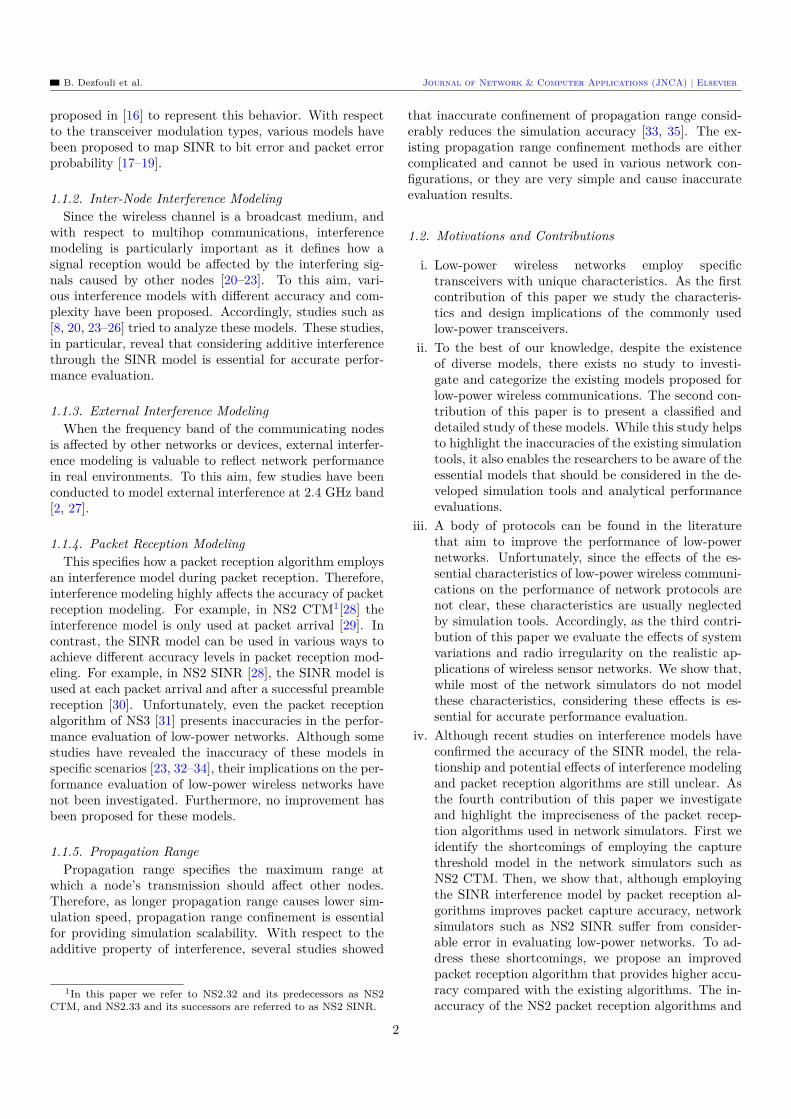
Journal of Network & Computer Applications (2014) Modeling Low-Power Wireless Communications Behnam Dezfouli 1,* , Marjan Radi 1 , S. A. Razak 1 , Tan Hwee-Pink 2 , K. A. Bakar 1 1 Department of Computer Science, Faculty of Computing, Universiti Teknologi Malaysia (UTM), Malaysia 2 Networking Protocols Department, Institute for Infocomm Research (I 2 R), Singapore Abstract Low-power wireless communications has particular characteristics that highly affect the performance of network protocols. However, many of these essential characteristics have not been considered in the existing simulation platforms and analytical performance evaluation models. While this issue invalidates many of the reported evaluation results, it also impedes pre-deployment performance prediction and parameter adjustment. Accordingly, this paper studies, analyzes and proposes models for accurate modeling of low-power wireless communications. Our contributions are six-fold. First, we investigate the essential characteristics of low-power wireless transceivers. Second, we present a classified and detailed study on modeling signal propagation, noise floor, system variations and interference. Third, we highlight the importance and effects of system variations and radio irregularity on the real applications of wireless sensor networks. Fourth, we reveal the inaccuracy of the packet reception algorithms used in the existing simulators. Furthermore, we propose an improved packet reception algorithm and we confirm its accuracy through comparison with empirical results. Fifth, we propose an architecture to integrate and implement the models presented in this paper. Finally, we show that the transitional region can be employed by the simulators to confine the propagation range and improve simulation scalability. To the best of our knowledge this is the first work that reveals the essentials of accurate modeling and evaluation of low-power wireless communications. Keywords: Simulation, Evaluation, Accuracy, Implementation 1. Introduction A low-power wireless network is a collection of nodes with scarce energy, computational and communication re- sources. As the radio transceiver is the major source of energy consumption, low-power wireless networks employ low-power wireless transceivers, which usually provide low data rate (tens of kbps), low transmission range (tens of meters) and poor link quality [1–4]. Nowadays, low-power wireless networks such as wireless sensor networks are being used for various applications. Accordingly, the research community has paid significant attention to design protocols for these networks. However, as protocol development and evaluation through testbed is costly and time consuming, simulation is the widely used approach [5–8]. Meanwhile, due to the particular charac- teristics of low-power wireless communications [2, 9, 10], which highly affect the performance of network protocols, simulation reliability mainly depends on the accuracy of modeling wireless communications. Unfortunately, while significant study has been conducted on protocol design and improvement, considerably less attention has been paid to the importance of accurate performance evalua- tion. Therefore, when the simulation platform is not ac- curate, either the demonstrated performance cannot be * Corresponding author: Email address: [email protected] (Behnam Dezfouli) expected in real-world scenarios, or the effects of wireless channel and transceiver on protocol performance are un- clear. 1.1. State-of-the-Art The accuracy of modeling wireless communications mainly depends on the following issues: (i) signal propa- gation and hardware modeling ; (ii) inter-node interference modeling ; (iii) external interference modeling ; (iv) packet reception modeling ; (v) propagation range. 1.1.1. Signal Propagation and Hardware Modeling Motivated by the observations of [8, 11–13], which in- validate the existence of a fixed and circular transmission range for all the nodes, various models have been pro- posed for multipath effect, radio irregularity, hardware heterogeneity and bit error rate. In particular, the stud- ies reported in [10, 14] confirmed the accuracy of the log- normal shadowing model to represent the link variations caused by multipath channel. In addition, these works investigate hardware heterogeneity in terms of transmis- sion power and noise floor differences for similar nodes. The results presented in [12] and [15] showed the existence of radio irregularity around low-power transmitters. This property reveals the significant variations of received sig- nal power versus direction changes around a transmitter. Accordingly, the radio irregularity model (RIM) has been 1084-8045/ c 2014 Elsevier Ltd. All rights reserved. DOI: http://dx.doi.org/10.1016/j.jnca.2014.02.009 1
Transcript of MODELING LOW-POWER WIRELESS COMMUNICATIONS
Journal of Network & Computer Applications (2014)
Modeling Low-Power Wireless Communications
Behnam Dezfouli1,∗, Marjan Radi1, S. A. Razak1, Tan Hwee-Pink2, K. A. Bakar1
1Department of Computer Science, Faculty of Computing, Universiti Teknologi Malaysia (UTM), Malaysia2Networking Protocols Department, Institute for Infocomm Research (I2R), Singapore
Abstract
Low-power wireless communications has particular characteristics that highly affect the performance of network protocols.However, many of these essential characteristics have not been considered in the existing simulation platforms andanalytical performance evaluation models. While this issue invalidates many of the reported evaluation results, it alsoimpedes pre-deployment performance prediction and parameter adjustment. Accordingly, this paper studies, analyzesand proposes models for accurate modeling of low-power wireless communications. Our contributions are six-fold. First,we investigate the essential characteristics of low-power wireless transceivers. Second, we present a classified and detailedstudy on modeling signal propagation, noise floor, system variations and interference. Third, we highlight the importanceand effects of system variations and radio irregularity on the real applications of wireless sensor networks. Fourth, wereveal the inaccuracy of the packet reception algorithms used in the existing simulators. Furthermore, we propose animproved packet reception algorithm and we confirm its accuracy through comparison with empirical results. Fifth,we propose an architecture to integrate and implement the models presented in this paper. Finally, we show that thetransitional region can be employed by the simulators to confine the propagation range and improve simulation scalability.To the best of our knowledge this is the first work that reveals the essentials of accurate modeling and evaluation oflow-power wireless communications.
Keywords: Simulation, Evaluation, Accuracy, Implementation
1. Introduction
A low-power wireless network is a collection of nodeswith scarce energy, computational and communication re-sources. As the radio transceiver is the major source ofenergy consumption, low-power wireless networks employlow-power wireless transceivers, which usually provide lowdata rate (tens of kbps), low transmission range (tens ofmeters) and poor link quality [1–4].
Nowadays, low-power wireless networks such as wirelesssensor networks are being used for various applications.Accordingly, the research community has paid significantattention to design protocols for these networks. However,as protocol development and evaluation through testbed iscostly and time consuming, simulation is the widely usedapproach [5–8]. Meanwhile, due to the particular charac-teristics of low-power wireless communications [2, 9, 10],which highly affect the performance of network protocols,simulation reliability mainly depends on the accuracy ofmodeling wireless communications. Unfortunately, whilesignificant study has been conducted on protocol designand improvement, considerably less attention has beenpaid to the importance of accurate performance evalua-tion. Therefore, when the simulation platform is not ac-curate, either the demonstrated performance cannot be
∗Corresponding author:Email address: [email protected] (Behnam Dezfouli)
expected in real-world scenarios, or the effects of wirelesschannel and transceiver on protocol performance are un-clear.
1.1. State-of-the-ArtThe accuracy of modeling wireless communications
mainly depends on the following issues: (i) signal propa-gation and hardware modeling; (ii) inter-node interferencemodeling; (iii) external interference modeling; (iv) packetreception modeling; (v) propagation range.
1.1.1. Signal Propagation and Hardware ModelingMotivated by the observations of [8, 11–13], which in-
validate the existence of a fixed and circular transmissionrange for all the nodes, various models have been pro-posed for multipath effect, radio irregularity, hardwareheterogeneity and bit error rate. In particular, the stud-ies reported in [10, 14] confirmed the accuracy of the log-normal shadowing model to represent the link variationscaused by multipath channel. In addition, these worksinvestigate hardware heterogeneity in terms of transmis-sion power and noise floor differences for similar nodes.The results presented in [12] and [15] showed the existenceof radio irregularity around low-power transmitters. Thisproperty reveals the significant variations of received sig-nal power versus direction changes around a transmitter.Accordingly, the radio irregularity model (RIM) has been
1084-8045/ c©2014 Elsevier Ltd. All rights reserved.DOI: http://dx.doi.org/10.1016/j.jnca.2014.02.009
1
B. Dezfouli et al. Journal of Network & Computer Applications (JNCA) | Elsevier
proposed in [16] to represent this behavior. With respectto the transceiver modulation types, various models havebeen proposed to map SINR to bit error and packet errorprobability [17–19].
1.1.2. Inter-Node Interference ModelingSince the wireless channel is a broadcast medium, and
with respect to multihop communications, interferencemodeling is particularly important as it defines how asignal reception would be affected by the interfering sig-nals caused by other nodes [20–23]. To this aim, vari-ous interference models with different accuracy and com-plexity have been proposed. Accordingly, studies such as[8, 20, 23–26] tried to analyze these models. These studies,in particular, reveal that considering additive interferencethrough the SINR model is essential for accurate perfor-mance evaluation.
1.1.3. External Interference ModelingWhen the frequency band of the communicating nodes
is affected by other networks or devices, external interfer-ence modeling is valuable to reflect network performancein real environments. To this aim, few studies have beenconducted to model external interference at 2.4 GHz band[2, 27].
1.1.4. Packet Reception ModelingThis specifies how a packet reception algorithm employs
an interference model during packet reception. Therefore,interference modeling highly affects the accuracy of packetreception modeling. For example, in NS2 CTM1[28] theinterference model is only used at packet arrival [29]. Incontrast, the SINR model can be used in various ways toachieve different accuracy levels in packet reception mod-eling. For example, in NS2 SINR [28], the SINR model isused at each packet arrival and after a successful preamblereception [30]. Unfortunately, even the packet receptionalgorithm of NS3 [31] presents inaccuracies in the perfor-mance evaluation of low-power networks. Although somestudies have revealed the inaccuracy of these models inspecific scenarios [23, 32–34], their implications on the per-formance evaluation of low-power wireless networks havenot been investigated. Furthermore, no improvement hasbeen proposed for these models.
1.1.5. Propagation RangePropagation range specifies the maximum range at
which a node’s transmission should affect other nodes.Therefore, as longer propagation range causes lower sim-ulation speed, propagation range confinement is essentialfor providing simulation scalability. With respect to theadditive property of interference, several studies showed
1In this paper we refer to NS2.32 and its predecessors as NS2CTM, and NS2.33 and its successors are referred to as NS2 SINR.
that inaccurate confinement of propagation range consid-erably reduces the simulation accuracy [33, 35]. The ex-isting propagation range confinement methods are eithercomplicated and cannot be used in various network con-figurations, or they are very simple and cause inaccurateevaluation results.
1.2. Motivations and Contributions
i. Low-power wireless networks employ specifictransceivers with unique characteristics. As the firstcontribution of this paper we study the characteris-tics and design implications of the commonly usedlow-power transceivers.
ii. To the best of our knowledge, despite the existenceof diverse models, there exists no study to investi-gate and categorize the existing models proposed forlow-power wireless communications. The second con-tribution of this paper is to present a classified anddetailed study of these models. While this study helpsto highlight the inaccuracies of the existing simulationtools, it also enables the researchers to be aware of theessential models that should be considered in the de-veloped simulation tools and analytical performanceevaluations.
iii. A body of protocols can be found in the literaturethat aim to improve the performance of low-powernetworks. Unfortunately, since the effects of the es-sential characteristics of low-power wireless communi-cations on the performance of network protocols arenot clear, these characteristics are usually neglectedby simulation tools. Accordingly, as the third contri-bution of this paper we evaluate the effects of systemvariations and radio irregularity on the realistic ap-plications of wireless sensor networks. We show that,while most of the network simulators do not modelthese characteristics, considering these effects is es-sential for accurate performance evaluation.
iv. Although recent studies on interference models haveconfirmed the accuracy of the SINR model, the rela-tionship and potential effects of interference modelingand packet reception algorithms are still unclear. Asthe fourth contribution of this paper we investigateand highlight the impreciseness of the packet recep-tion algorithms used in network simulators. First weidentify the shortcomings of employing the capturethreshold model in the network simulators such asNS2 CTM. Then, we show that, although employingthe SINR interference model by packet reception al-gorithms improves packet capture accuracy, networksimulators such as NS2 SINR suffer from consider-able error in evaluating low-power networks. To ad-dress these shortcomings, we propose an improvedpacket reception algorithm that provides higher accu-racy compared with the existing algorithms. The in-accuracy of the NS2 packet reception algorithms and
2
B. Dezfouli et al. Journal of Network & Computer Applications (JNCA) | Elsevier
the significantly higher accuracy of the proposed al-gorithm are demonstrated through comparison withempirical results.
v. Since none of the existing simulation tools implementall the essential models required for evaluating low-power networks, the fifth contribution of this paper isto propose an architecture within which these mod-els can be implemented. This architecture along withthe proposed packet reception algorithm is used to de-velop an accurate simulation tool on the OMNeT++simulation framework. We also discuss about the ef-fect of each model on simulation speed.
vi. As the sixth contribution of this paper, we studythe existing approaches used by the simulation toolsto improve simulation speed through reducing theoverhead of signal propagation. Using the devel-oped simulation tool, we change the radio propagationrange and measure its effects on performance evalua-tion. Through comparison with the existing models,we show that the transitional region size provides astraightforward way to confine the propagation range.
1.3. Paper OrganizationIn Section 2, we study the important characteristics of
low-power transceivers. Section 3 presents the models re-quired for accurate performance evaluation. We describethe methodology employed for performance evaluations inSection 4. Section 5 presents the analyses that reflect theimportance and effects of modeling system variations andradio irregularity. In Section 6 we carefully analyze thepacket reception algorithms used by NS2. We also pro-pose an improved packet reception algorithm. In Section7 we present an architecture to integrate and implementthe essential models of simulating wireless networks. Ad-ditionally, we evaluate the effects of propagation range.Table 1 summarizes the key notations used in this paper.
2. Low-Power RF Transceivers
In this section, we study the characteristics of low-powerwireless transceivers. Table 2 presents the main featuresof five transceivers. Since CC1000 and CC2420 are the ra-dios employed by the commonly used wireless sensor nodes(such as Mica2 [36], MicaZ [37], and TelosB [38]), we pro-vide additional explanations regarding these transceivers.
2.1. Signal SynchronizationIn low-power wireless communications, regardless of the
utilized transceiver module, receiver should obtain certaininformation about the incoming signal before receivingdata. To this aim, data packets begin with a predefinedtraining sequence, called preamble, which enables the re-ceiver to learn about the parameters of the transmitter. Inaddition to the preamble bytes, the receiver should be ableto detect the start and end of the data frame. Therefore,specific bytes should be transmitted immediately after the
preamble bytes. These bytes are called sync word or startof frame delimiter (SFD). The total duration of the pream-ble and sync bytes is usually referred to as the physical-layer header. To achieve accurate synchronization, eachradio defines a minimum number of bits that should bereceived before actual data reception. In this paper, theminimum number of synchronization bits located at theend of the preamble is referred to as the settling bits.
CC1000. As this is a byte-base radio (cf. Section 2.2),the size and pattern of the preamble bits can be config-ured by the user. However, the minimum preamble sizedepends on the configured acquisition mode and receiversensitivity. For example, to achieve the highest sensitivitylevel in Manchester mode, preamble duration should be atleast 98 bits long. To satisfy this requirement, the imple-mentation of B-MAC [42] in TinyOS [43] uses 10 bytes asthe physical-layer header.
CC2420. The default preamble size is 4 bytes, whichprovides compatibility with the IEEE 802.15.4 standard[18]. In addition, it is recommended to avoid using pream-bles shorter than 4 bytes, because it may increase the num-ber of false packet detections.
Although using the minimum required preamble sizereduces the overhead of packet transmission, low-powerMAC protocols usually employ the low-power listeningmechanism (LPL) [42, 44], which requires using largepreambles. For example, while the required number ofsettling bits for CC1000 radio is about 6 bytes, B-MACwith 200 ms sampling interval uses 480-byte preambles.In this case, even if a signal’s SINR value is not strongenough during the first 474 bytes of the preamble, pro-viding enough SINR value during the last 6 bytes of thepreamble can result in successful synchronization. We willlater show that employing long preambles requires specificdesign considerations regarding packet reception modeling(cf. Section 6).
2.2. Packet FormattingBased on the packet formatting mechanism, the exist-
ing low-power RF transceivers can be categorized intotwo groups: byte-oriented and packet-oriented. A byte-oriented radio (e.g., CC1000) does not provide any packetformatting mechanism by the radio’s hardware. Hence, inaddition to the data bytes, microcontroller should gener-ate and transmit the preamble, sync word and CRC bitsinto the radio module. As the radio merely transmits thedata received from the microcontroller, every transmittedbit can be controlled by the user. Therefore, by using byte-oriented radios, protocol designers can easily define theirown packet format, based on the requirements of upper-layer protocols. The hardware of packet-oriented radios(e.g., CC2420) defines a specific packet format that usu-ally follows a specific standard (e.g., 802.15.4). Althoughthese radios allow new packet format definition, the pro-vided flexibility is less than that provided by byte-orientedradios. For example, as packet-based radios define a max-imum packet length imposed by their transmission buffer,
3
B. Dezfouli et al. Journal of Network & Computer Applications (JNCA) | Elsevier
Table 1: A summary of key notationsDescription SymbolA signal transmitted by node i Si
The set of the signals currently being received at a node SOutput power of node i Ωi
Output power of node i considering hardware heterogeneity Ωadji
Received power at node j, corresponding to signal Si Ψj(Si)Average noise floor ΨNoise floor of node i considering hardware heterogeneity Ψadj
iMAC protocol data unit (MAC header+payload+CRC) MPDUNumber of required bits for signal synchronization LsettlingNumber of MPDU bits LMPDUTotal number of bits in a packet LpacketSINR value corresponding to signal Si SINR(Si)SINR value at node j, corresponding to signal Si , at time t SINRj(Si, t)The set of nodes in the network VRadio speed RPath-loss exponent ηStandard deviation of multipath channel variations σch
Standard deviation of additive white Gaussian noise σW GN
Standard deviation of transmission power heterogeneity σtx
Standard deviation of noise floor heterogeneity σrx
it may be infeasible to achieve a desired preamble dura-tion, which is required for LPL-based MAC protocols. Inthis case, multiple packets can be transmitted to act as along preamble and wake up the receiver [45]. On the otherhand, new radios (such as CC2500) provide some featuresto support the LPL mechanism.
CC1000. This radio does not provide any data buffer.Therefore, despite its packet formatting flexibility, findingthe SFD bytes to identify actual data bytes should be im-plemented by software.
CC2420. Although it supports the 802.15.4-compliantpacket format, it also allows for packet formatting. How-ever, as this transceiver provides two separate 128-bytememory banks for packet transmission and reception, itdoes not support packet sizes larger than 127 bytes (onebyte is reserved for packet size).
2.3. Modulation Types
Wireless transceivers can be categorized based on theirmodulation type: narrowband and wideband. While nar-rowband radios can achieve longer transmission range withlower energy consumption, wideband radios spend moreenergy, because they spread the signal over a wider rangeto provide higher interference immunity. Additionally,since wideband radios provide higher data rate, they op-erate at 2.4 GHz due to the larger available bandwidth.
CC1000. This transceiver can be configured to operateat frequency range 300-1000 MHz, with different transmis-sion and reception frequencies. The very fast frequencyshifting capability of this radio makes it suitable for im-plementing frequency hopping protocols.
CC2420. In compliance with the 802.15.4 standard,CC2420 can be programmed to operate at 16 differentchannels, numbered from 11 to 26. Therefore, its mul-tichannel capability can be utilized by the MAC protocolsto increase network throughput. Although CC2420 uses
the Direct Sequence Spread Spectrum (DSSS) modulation,studies showed that most of the channels suffer from signif-icant interference from other 2.4 GHz transmitters [27, 46](cf. Section 3.8).
2.4. The Capture Effect
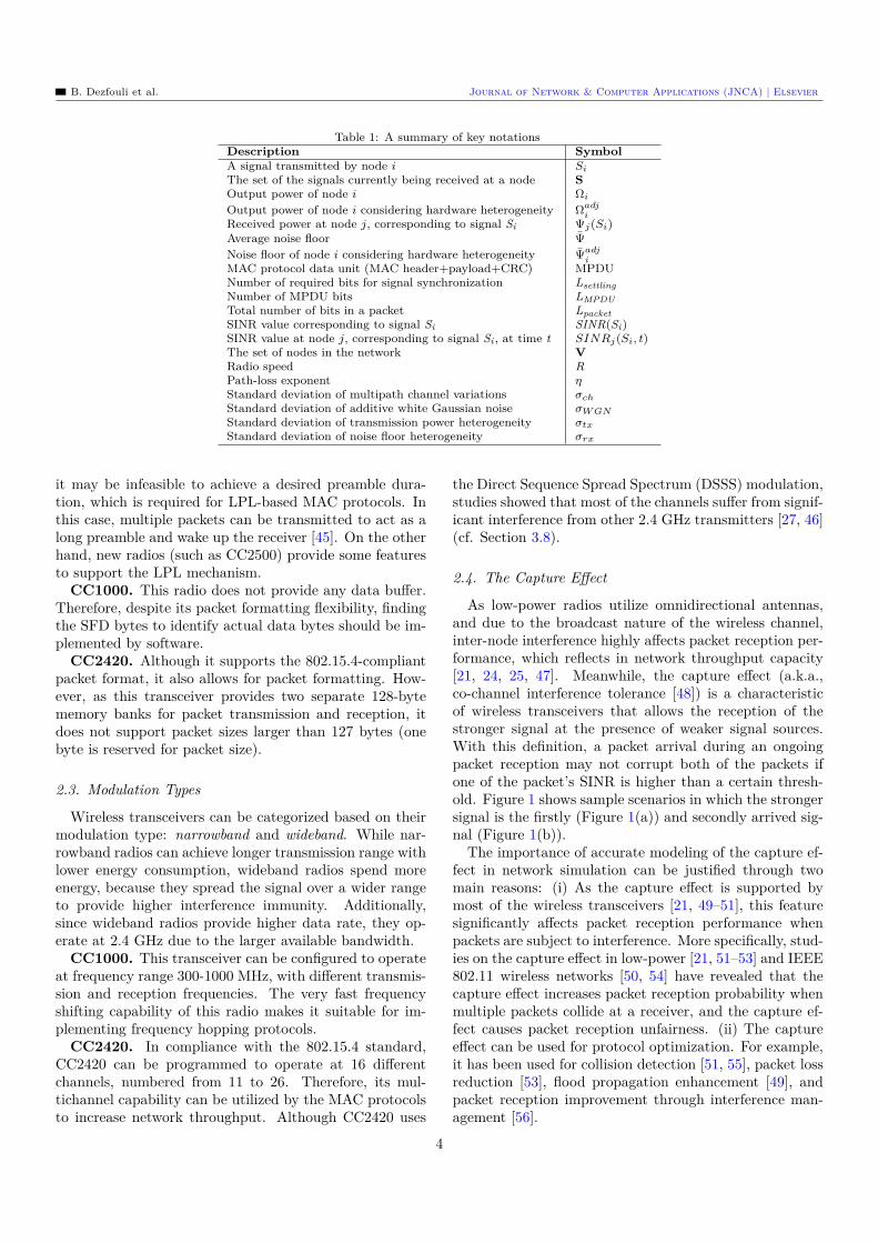
As low-power radios utilize omnidirectional antennas,and due to the broadcast nature of the wireless channel,inter-node interference highly affects packet reception per-formance, which reflects in network throughput capacity[21, 24, 25, 47]. Meanwhile, the capture effect (a.k.a.,co-channel interference tolerance [48]) is a characteristicof wireless transceivers that allows the reception of thestronger signal at the presence of weaker signal sources.With this definition, a packet arrival during an ongoingpacket reception may not corrupt both of the packets ifone of the packet’s SINR is higher than a certain thresh-old. Figure 1 shows sample scenarios in which the strongersignal is the firstly (Figure 1(a)) and secondly arrived sig-nal (Figure 1(b)).
The importance of accurate modeling of the capture ef-fect in network simulation can be justified through twomain reasons: (i) As the capture effect is supported bymost of the wireless transceivers [21, 49–51], this featuresignificantly affects packet reception performance whenpackets are subject to interference. More specifically, stud-ies on the capture effect in low-power [21, 51–53] and IEEE802.11 wireless networks [50, 54] have revealed that thecapture effect increases packet reception probability whenmultiple packets collide at a receiver, and the capture ef-fect causes packet reception unfairness. (ii) The captureeffect can be used for protocol optimization. For example,it has been used for collision detection [51, 55], packet lossreduction [53], flood propagation enhancement [49], andpacket reception improvement through interference man-agement [56].
4
B. Dezfouli et al. Journal of Network & Computer Applications (JNCA) | Elsevier
Table 2: Low-power RF transceivers and their characteristicsTransceiver TR1000 [39] CC1000 [4] CC1120 [40] CC2420 [3] CC2500 [41]Radio Type Narrowband Narrowband Narrowband Wideband WidebandByte/Packet Ori-ented Byte Oriented Byte Oriented Packet Oriented Packet Oriented Packet Oriented
Operating Fre-quency 916/868 MHz 315/433/868/916
MHz
170/315/433/868/915/920/950 MHz
2.4 GHz 2.4 GHz
Max Data Rate[kbps] 115.2 76.8 200 250 500
Modulation OOK/ASK FSK2-FSK/2-GFSK/4-FSK/4-GFSK/MSK/ OOK
DSSS-O-QPSK OOK/2-FSK/GFSK/MSK
Output Power[dBm] 1.5 -20 to 10 -40 to 16 -24 to 0 -30 to 0
TX Power [mA] 12 (1.5 dBm)
10.4(0 dBm, 433 MHz)16.5(0 dBm, 868 MHz)
26(0 dBm, 950MHz)
17.4 (0 dBm)8.5 (-25 dBm)
21.2 (0 dBm)11.1 (-12 dBm)
RX Power [mA]3 (2.4 kbps)3.8 (115.2kbps)
7.4 (433 MHz)9.6 (868 MHz) 22 19.7 12.8 (2.4kbps)
19.6 (500kbps)
Sleep Power [µA] 0.7 0.2 to 1 0.3 to 1 1 0.4
Startup Time [ms] 0.016 2 0.4
0.86,0.3(power ramp-uptime)
0.3,5(power ramp-uptime)
Receiver Sensitivity(Best) [dBm]
-106(2.4 kbps,ASK)
-110(1.2 kbps, 433MHz)
-127 (300 bps)-103 (200 kps)
-94,-85 for 802.15.4
-104(2.4 kbps, FSK)
3. Modeling Low-Power Wireless Communications
The aim of this section is to present the essential charac-teristics of low-power wireless communications, as well asthe models proposed for these characteristics. Accordingly,we study the existing models proposed for radio propaga-tion, bit error computation and interference.
3.1. Signal PropagationA signal sent by a wireless transmitter loses its power
as it moves away from the sender. The three well-knownmodels of signal decay are [17]: (i) free-space propagationmodel, (ii) ground reflection (two-ray) model, and (ii) log-normal shadowing model (which is an elaboration over thelog-distance path-loss model).
Although the ground reflection model includes the ef-fects of ground reflection path and provides higher accu-racy than the free-space propagation model, both of thesemodels represent signal strength as a fixed function of dis-tance. This representation results in a circular communi-cation range, which is referred to as the unit disk graphmodel (UDG). However, experimental evaluation of low-power links indicates the existence of three distinct regionsaround a sender [9, 10, 57, 58]: connected (packet recep-tion ratio is higher than 90%), transitional (packet recep-tion ratio varies between 90% to 10%), and disconnected(packet reception ratio is lower than 10%). Therefore, theUDG model has been criticized by the researchers, becausethe theoretical and simulation-based performance evalua-tion of the protocols designed with this assumption are dif-ferent from the expected real-world results [11, 12, 58, 59].In contrast to the free-space and ground reflection mod-els, the log-normal shadowing model includes the effects of
multipath propagation and represents signal strength at agiven distance as a random variable. Specifically, Nikookarand Hashemi [60] showed that the log-normal distributionprovides a more accurate multipath fading model thanthe Rayleigh and Nakagami distributions. The log-normalshadowing model is,
PL(d) = PL(d0) + 10ηlog10( d
d0) + N(0, σch) (1)
where d is the distance from the sender, PL(d) is thepath loss at distance d, d0 is the reference distance (a.k.a.,close-in distance), PL(d0) is the path loss at the referencedistance, η is the path-loss exponent, N(0, σch) is a zero-mean Gaussian random variable with standard deviationσch, and σch is the variations of signal power due to themultipath channel. It has been shown that this equationholds for both indoor and outdoor environments [14, 17].
Sohrabi et al. [61] conducted extensive experiments todetermine channel parameters for the log-normal shadow-ing model in the frequency range 800-1000 MHz for dif-ferent environments. Their results indicate path-loss ex-ponent from η=1.9 (for a multi-leveled engineering build-ing) to η=5 (for a bamboo jungle). They also showed 30to 50 dB loss in signal power at the reference distance 1meter. Similar experiments have also been conducted byZuniga and Krishnamachari [10, 14] to obtain the chan-nel parameters using CC1000 radio in indoor and outdoorenvironments. Although the general validity of the log-normal shadowing model has been confirmed for varioustransceivers [10, 62, 63], specific parameters should be usedfor each radio. For example, in a given environment, thelog-normal shadowing model requires different parametersfor CC1000 and CC2420 transceivers, which is due to the
5
B. Dezfouli et al. Journal of Network & Computer Applications (JNCA) | Elsevier
3 3.5 4 4.5 5 5.5 6 6.5 70
10
20
30
40
50
60
70CC1000
Dis
tance
from
Sen
der
[m]
Path Loss (η)(a)
Connected RegionTransitional Region
1 1.5 2 2.5 3 3.5 4 4.5 5 5.5 60
5
10
15
20
25
30CC1000
Dis
tance
from
Sen
der
[m]
Multi-Path (σch)(b)
Connected RegionTransitional Region
3 3.5 4 4.5 5 5.5 6 6.5 70
50
100
150
200CC2420
Dis
tance
from
Sen
der
[m]
Path Loss (η)(c)
Connected RegionTransitional Region
1 1.5 2 2.5 3 3.5 4 4.5 5 5.5 60
10
20
30
40
50
60
70CC2420
Dis
tance
from
Sen
der
[m]
Multi-Path (σch)(d)
Connected RegionTransitional Region
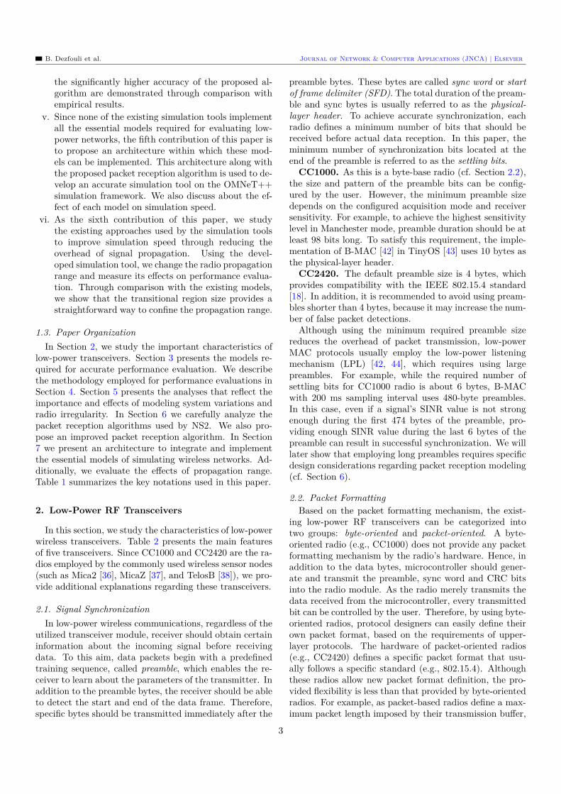
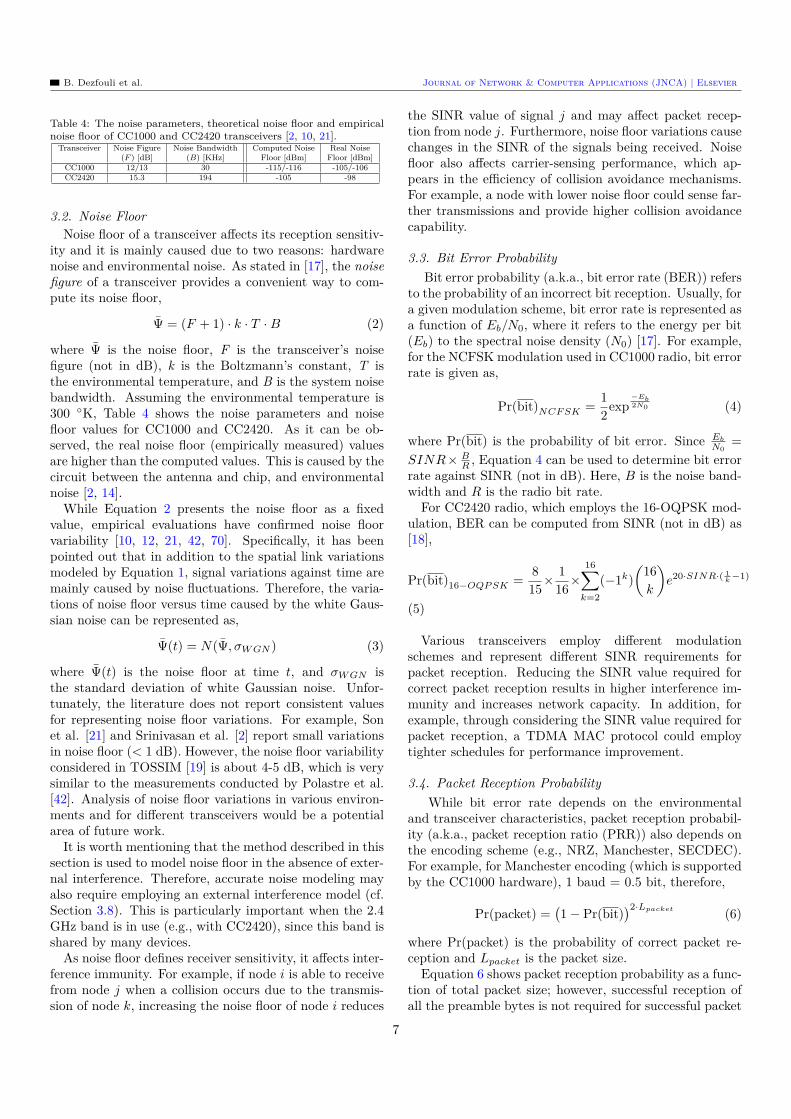
Figure 2: Effects of path-loss exponent and multipath variations on the extent of the connected and transitional region for CC1000 andCC2420 transceivers. In figure (a) and (c) the multipath value is 4. In figure (b) and (d) the path-loss exponent is 4.
Settling
S1:
S2:
t0: SINR(S1,t0)= Ψ(S1) / Ψ > SINRth
t1: SINR(S2,t1) =
Ψ(S2) / (Ψ + Ψ(S1)) < SINRth
Settling
t1: SINR(S1,t1) = Ψ(S1) / (Ψ + Ψ(S2)) > SINRth
Settling
t0: SINR(S1,t0) =
Ψ(S1) / Ψ > SINRth Settling
t1: SINR(S1,t1) = Ψ(S1) / (Ψ + Ψ(S2)) < SINRth
t1: SINR(S2,t1) = Ψ(S2) / (Ψ + Ψ(S1)) > SINRth
(a)
(b)
S1:
S2:
MPDU
MPDU
MPDU
MPDU
Preamble
Preamble
Preamble
Preamble
Figure 1: (a) Strongest-first packet capture: packet S1 can be com-pletely received, because its SINR is higher than the threshold valueeven after the arrival of S2. (b) Stronger-last packet capture: al-though the radio is receiving packet S1 during t0 to t1, it switches toreceive S2 at time t1, because the SINR of this signal is higher thanS1, and it is higher than the threshold value.
differences in the frequency and modulation types used inthese transceivers. Table 3 summarizes the parameters ofthe log-normal shadowing model for CC1000 and CC2420radios.
Using Equation 1, Figure 2 shows how path-loss expo-nent and multipath variations affect the size of the con-nected and transitional regions. The main observationsfrom this figure are: Firstly, for a given multipath value,reducing the path-loss exponent results in significantlyhigher increase in the transitional region size, comparedwith the connected region size. Therefore, as Table 3 indi-
Table 3: The parameters of the log-normal shadowing model forCC1000 and CC2420 radios and for different environments [10, 19,62, 64–66].
EnvironmentIndoor Outdoor
CC1000P L(1) 52.1 55.4
η 3.3 (2.1-4.5) 4.7 (4.3-5.1)σch 5.5 (4.6-6.8) 3.2 (2.6-3.8)
Hallway Office Parking Lawn Forrest
CC2420P L(2) 53.9 49.9 59.2 56.4 57.4
η 1.82 1.97 3 3.6 2.08σch 5.5 (4.6-6.8) 3.2 (2.6-3.8)
cates lower path-loss exponent for the CC2420 radio, thisradio causes larger transitional region and more numberof links with poor quality. Secondly, for a given path-lossexponent, increasing the multipath variations results inlower size of the connected region and larger size of thetransitional region. Section 5.1 provides further studiesregarding the effects of system variations on the perfor-mance of wireless sensor networks.
The importance of employing an accurate signal propa-gation model is intuitive. For example, the effects of theconstant and variable part of the log-normal shadowingmodel can be discussed as follows. First, the fixed part(i.e., PL(d0) + 10ηlog10( d
d0)) highly affects signal relation-
ship between nodes. As signal relationship between nodesdetermines network capacity, accurate path-loss model-ing is crucial. Second, the variable part (i.e., N(0, σch))models signal variations, which also affects signal relation-ship between nodes. More specifically, as this part con-tributes to SINR variations during packet reception, it af-fects packet reception performance. Both parts of the log-normal shadowing model influence higher-layer protocolssuch as MAC and routing. For example, higher multipathvariation increases the number of hops to the sink node, asFigure 2 and Section 5.1 show. Additionally, for example,signal variations affect carrier-sensing performance.
The log-normal shadowing model has widely been uti-lized in the low-power wireless networking literature formathematical analysis, protocol design, protocol evalua-tion, etc. [6, 59, 62, 67–69]. Furthermore, this model hasbeen used in many of the wireless network simulators.
6
B. Dezfouli et al. Journal of Network & Computer Applications (JNCA) | Elsevier
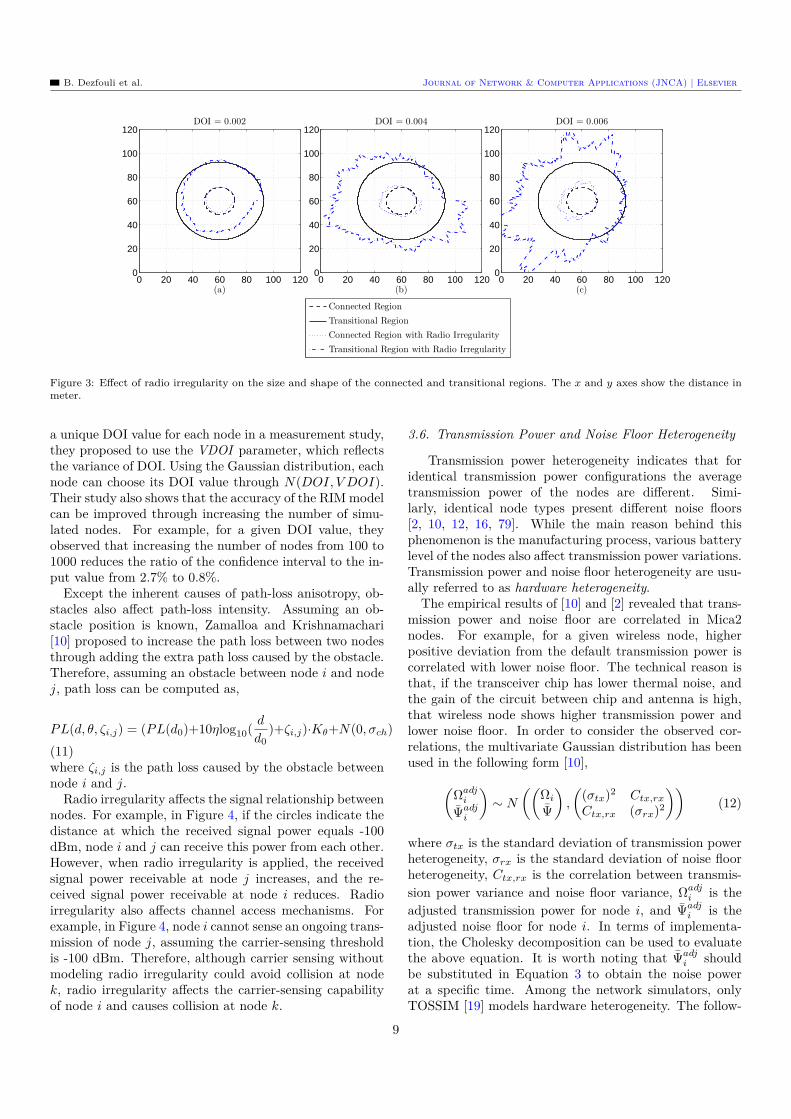
Table 4: The noise parameters, theoretical noise floor and empiricalnoise floor of CC1000 and CC2420 transceivers [2, 10, 21].
Transceiver Noise Figure Noise Bandwidth Computed Noise Real Noise(F ) [dB] (B) [KHz] Floor [dBm] Floor [dBm]
CC1000 12/13 30 -115/-116 -105/-106CC2420 15.3 194 -105 -98
3.2. Noise FloorNoise floor of a transceiver affects its reception sensitiv-
ity and it is mainly caused due to two reasons: hardwarenoise and environmental noise. As stated in [17], the noisefigure of a transceiver provides a convenient way to com-pute its noise floor,
Ψ = (F + 1) · k · T · B (2)
where Ψ is the noise floor, F is the transceiver’s noisefigure (not in dB), k is the Boltzmann’s constant, T isthe environmental temperature, and B is the system noisebandwidth. Assuming the environmental temperature is300 K, Table 4 shows the noise parameters and noisefloor values for CC1000 and CC2420. As it can be ob-served, the real noise floor (empirically measured) valuesare higher than the computed values. This is caused by thecircuit between the antenna and chip, and environmentalnoise [2, 14].
While Equation 2 presents the noise floor as a fixedvalue, empirical evaluations have confirmed noise floorvariability [10, 12, 21, 42, 70]. Specifically, it has beenpointed out that in addition to the spatial link variationsmodeled by Equation 1, signal variations against time aremainly caused by noise fluctuations. Therefore, the varia-tions of noise floor versus time caused by the white Gaus-sian noise can be represented as,
Ψ(t) = N(Ψ, σW GN ) (3)
where Ψ(t) is the noise floor at time t, and σW GN isthe standard deviation of white Gaussian noise. Unfor-tunately, the literature does not report consistent valuesfor representing noise floor variations. For example, Sonet al. [21] and Srinivasan et al. [2] report small variationsin noise floor (< 1 dB). However, the noise floor variabilityconsidered in TOSSIM [19] is about 4-5 dB, which is verysimilar to the measurements conducted by Polastre et al.[42]. Analysis of noise floor variations in various environ-ments and for different transceivers would be a potentialarea of future work.
It is worth mentioning that the method described in thissection is used to model noise floor in the absence of exter-nal interference. Therefore, accurate noise modeling mayalso require employing an external interference model (cf.Section 3.8). This is particularly important when the 2.4GHz band is in use (e.g., with CC2420), since this band isshared by many devices.
As noise floor defines receiver sensitivity, it affects inter-ference immunity. For example, if node i is able to receivefrom node j when a collision occurs due to the transmis-sion of node k, increasing the noise floor of node i reduces
the SINR value of signal j and may affect packet recep-tion from node j. Furthermore, noise floor variations causechanges in the SINR of the signals being received. Noisefloor also affects carrier-sensing performance, which ap-pears in the efficiency of collision avoidance mechanisms.For example, a node with lower noise floor could sense far-ther transmissions and provide higher collision avoidancecapability.
3.3. Bit Error ProbabilityBit error probability (a.k.a., bit error rate (BER)) refers
to the probability of an incorrect bit reception. Usually, fora given modulation scheme, bit error rate is represented asa function of Eb/N0, where it refers to the energy per bit(Eb) to the spectral noise density (N0) [17]. For example,for the NCFSK modulation used in CC1000 radio, bit errorrate is given as,
Pr(bit)NCF SK = 12exp
−Eb2N0 (4)
where Pr(bit) is the probability of bit error. Since Eb
N0=
SINR× BR , Equation 4 can be used to determine bit error
rate against SINR (not in dB). Here, B is the noise band-width and R is the radio bit rate.
For CC2420 radio, which employs the 16-OQPSK mod-ulation, BER can be computed from SINR (not in dB) as[18],
Pr(bit)16−OQP SK = 815× 1
16×16∑
k=2(−1k)
(16k
)e20·SINR·( 1
k −1)
(5)
Various transceivers employ different modulationschemes and represent different SINR requirements forpacket reception. Reducing the SINR value required forcorrect packet reception results in higher interference im-munity and increases network capacity. In addition, forexample, through considering the SINR value required forpacket reception, a TDMA MAC protocol could employtighter schedules for performance improvement.
3.4. Packet Reception ProbabilityWhile bit error rate depends on the environmental
and transceiver characteristics, packet reception probabil-ity (a.k.a., packet reception ratio (PRR)) also depends onthe encoding scheme (e.g., NRZ, Manchester, SECDEC).For example, for Manchester encoding (which is supportedby the CC1000 hardware), 1 baud = 0.5 bit, therefore,
Pr(packet) =(1 − Pr(bit)
)2·Lpacket (6)
where Pr(packet) is the probability of correct packet re-ception and Lpacket is the packet size.
Equation 6 shows packet reception probability as a func-tion of total packet size; however, successful reception ofall the preamble bytes is not required for successful packet
7
B. Dezfouli et al. Journal of Network & Computer Applications (JNCA) | Elsevier
reception. In particular, as low-power wireless networksusually employ long preambles to implement the LPL tech-nique, a packet may be received without complete recep-tion of its preamble bytes. With respect to the definitionsgiven in Section 2.1, the probability of correct packet re-ception can be given as,
Pr(packet) = (Pr(bit)settling)Lsettling ×(Pr(bit)MP DU )LMP DU
(7)where Pr(bit)settling is computed through considering theSINR value during the settling bits, and Pr(bit)MP DU iscomputed through considering the SINR value during theMPDU.
Computing bit error rate to decide about correct packetreception has been used in simulators such as GloMoSim[71], Castalia [72], NS3 [31] and MiXiM [73]. After com-puting Pr(packet) it is compared with a random numberin range [0,1] to determine packet reception status. Unfor-tunately, these simulators do not account for packet syn-chronization. In other words, successful packet receptiondepends on the correct reception of all the preamble bytes.Therefore, these simulator do not provide an accurate es-timation of packet reception performance. NS2 CTM andNS2 SINR do not compute bit error rate. Rather, a packetis received if its SINR is higher than a specific thresholdvalue. The threshold value is set based on empirical obser-vations. In TOSSIM [19], instead of computing bit errorrate based on transceiver specifications, an empirical traceis used to determine packet reception ratio. Specifically,TOSSIM employs the following function for SINR to PRRmapping,
Pr(packet) =(
1 − 12 erfc(a1 ×
√|SINR−a2|
2 ))2×23
(8)
where erfc is the complementary error function, a1 =1.3687 and a2 = 0.9187. Unfortunately, this function onlyfits the empirical results of using 23-byte packet, and can-not be used for other packet sizes.
Although this section provided a general overview ofpacket reception modeling, Section 6 presents further de-tails regarding the existing packet reception algorithms.
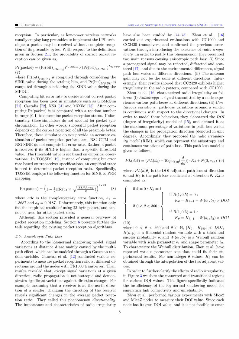
3.5. Anisotropic Path LossAccording to the log-normal shadowing model, signal
variations at distance d are mainly caused by the multi-path effect, which can be modeled through a Gaussian ran-dom variable. Ganesan et al. [12] conducted various ex-periments to measure packet reception ratio at different di-rections around the nodes with TR1000 transceiver. Theirresults revealed that, except signal variations at a givendirection, radio propagation is not isotropic and demon-strates significant variations against direction changes. Forexample, assuming that a receiver is at the north direc-tion of a sender, changing the direction of the receiverreveals significant changes in the average packet recep-tion ratio. They called this phenomenon directionality.The importance and characteristics of radio irregularity
have also been studied by [74–78]. Zhou et al. [16]carried out experimental evaluations with CC1000 andCC2420 transceivers, and confirmed the previous obser-vations through introducing the existence of radio irregu-larity. In order to justify this phenomenon, they presentedtwo main reasons causing anisotropic path loss: (i) Sincea propagated signal may be reflected, diffracted and scat-tered [17], and due to the environmental differences, signalpath loss varies at different directions. (ii) The antennagain may not be the same at different directions. Inter-estingly, their results showed that CC2420 exhibits higherirregularity in the radio pattern, compared with CC1000.
Zhou et al. [16] characterized radio irregularity as fol-lows: (i) Anisotropy: a signal transmitted by a node expe-riences various path losses at different directions; (ii) Con-tinuous variations: path-loss variations around a senderis continuous with respect to the directional changes. Inorder to model these behaviors, they elaborated the DOI(degree of irregularity) model of [15], and defined it asthe maximum percentage of variations in path loss versusthe changes in the propagation direction (denoted in unitdegree). Accordingly, they proposed the radio irregular-ity model (RIM), which can represent the anisotropy andcontinuous variations of path loss. This path-loss model isgiven as follows,
PL(d, θ) = (PL(d0) + 10ηlog10( d
d0)) · Kθ + N(0, σch) (9)
where PL(d, θ) is the DOI-adjusted path loss at directionθ, and Kθ is the path-loss coefficient at direction θ. Kθ iscomputed as,
if θ = 0 : Kθ = 1
if 0 < θ < 360 :
if B(1, 0.5) = 0 :Kθ = Kθ−1 + W (b1, b2) × DOI
if B(1, 0.5) = 1 :Kθ = Kθ−1 − W (b1, b2) × DOI
(10)where 0 < θ < 360 and θ ∈ N, |K0 − K359| < DOI,B(n, p) is a Binomial random variable with n trials andsuccess probability p, and W (b1, b2) is a Weibull randomvariable with scale parameter b1 and shape parameter b2.To characterize the Weibull distribution, Zhou et al. havereported various parameter sets that could fit their ex-perimental results. For non-integer θ values, Kθ can beobtained through the interpolation of the two adjacent val-ues.
In order to further clarify the effects of radio irregularity,in Figure 3 we show the connected and transitional regionsfor various DOI values. This figure specifically indicatesthe insufficiency of the log-normal shadowing model forsimulating link connectivity and unreliability.
Zhou et al. performed various experiments with Mica2and MicaZ nodes to measure their DOI value. Since eachnode has its own DOI value, and it is not feasible to enter
8
B. Dezfouli et al. Journal of Network & Computer Applications (JNCA) | Elsevier41
0 20 40 60 80 100 1200
20
40
60
80
100
120DOI = 0.002
(a)0 20 40 60 80 100 120
0
20
40
60
80
100
120DOI = 0.004
(b)0 20 40 60 80 100 120
0
20
40
60
80
100
120DOI = 0.006
(c)
Connected Region
Transitional Region
Connected Region with Radio Irregularity
Transitional Region with Radio Irregularity
Figure 2.11: Effect of radio irregularity on the size and shape of the connectedand transitional regions. The x and y axes show the distance in meter.
Zhou et al. performed various experiments with Mica2 and MicaZnodes to measure their DOI value. Since each node has its own DOI value, andit is not feasible to enter a unique DOI value for each node in a measurementstudy, they proposed to use the VDOI parameter, which reflects the varianceof DOI. Using the Gaussian distribution, each node can choose its DOI valuethrough N(DOI, V DOI).
Effect on Collisions. Since radio irregularity changes propagationrange, it affects the collision relationship between nodes. For example, in Figure2.12, if the circles indicate the distance at which the received signal powerequals -100 dBm, node A and node B can receive this power from each other.However, when radio irregularity is applied, the received signal power receivableat node B increases, and the received signal power receivable at node A reduces.From the collision avoidance point of view, radio irregularity affects channelaccess mechanisms. For example, in Figure 2.12, while node B is sending tonode C, node A cannot sense this transmission. Therefore, although carriersensing without modeling radio irregularity could avoid collision at node C, radioirregularity affects the carrier-sensing capability of node A and causes collisionat node C.
2.2.3.3 Transmission Power and Noise Floor Heterogeneity
Transmission power heterogeneity indicates that for identical transmissionpower configurations the average transmission power of the nodes are different
Figure 3: Effect of radio irregularity on the size and shape of the connected and transitional regions. The x and y axes show the distance inmeter.
a unique DOI value for each node in a measurement study,they proposed to use the VDOI parameter, which reflectsthe variance of DOI. Using the Gaussian distribution, eachnode can choose its DOI value through N(DOI, V DOI).Their study also shows that the accuracy of the RIM modelcan be improved through increasing the number of simu-lated nodes. For example, for a given DOI value, theyobserved that increasing the number of nodes from 100 to1000 reduces the ratio of the confidence interval to the in-put value from 2.7% to 0.8%.
Except the inherent causes of path-loss anisotropy, ob-stacles also affect path-loss intensity. Assuming an ob-stacle position is known, Zamalloa and Krishnamachari[10] proposed to increase the path loss between two nodesthrough adding the extra path loss caused by the obstacle.Therefore, assuming an obstacle between node i and nodej, path loss can be computed as,
PL(d, θ, ζi,j) = (PL(d0)+10ηlog10( d
d0)+ζi,j)·Kθ+N(0, σch)
(11)where ζi,j is the path loss caused by the obstacle betweennode i and j.
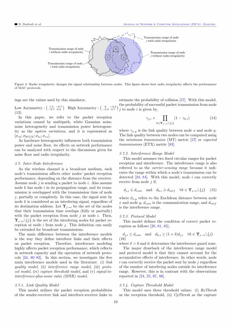
Radio irregularity affects the signal relationship betweennodes. For example, in Figure 4, if the circles indicate thedistance at which the received signal power equals -100dBm, node i and j can receive this power from each other.However, when radio irregularity is applied, the receivedsignal power receivable at node j increases, and the re-ceived signal power receivable at node i reduces. Radioirregularity also affects channel access mechanisms. Forexample, in Figure 4, node i cannot sense an ongoing trans-mission of node j, assuming the carrier-sensing thresholdis -100 dBm. Therefore, although carrier sensing withoutmodeling radio irregularity could avoid collision at nodek, radio irregularity affects the carrier-sensing capabilityof node i and causes collision at node k.
3.6. Transmission Power and Noise Floor Heterogeneity
Transmission power heterogeneity indicates that foridentical transmission power configurations the averagetransmission power of the nodes are different. Simi-larly, identical node types present different noise floors[2, 10, 12, 16, 79]. While the main reason behind thisphenomenon is the manufacturing process, various batterylevel of the nodes also affect transmission power variations.Transmission power and noise floor heterogeneity are usu-ally referred to as hardware heterogeneity.
The empirical results of [10] and [2] revealed that trans-mission power and noise floor are correlated in Mica2nodes. For example, for a given wireless node, higherpositive deviation from the default transmission power iscorrelated with lower noise floor. The technical reason isthat, if the transceiver chip has lower thermal noise, andthe gain of the circuit between chip and antenna is high,that wireless node shows higher transmission power andlower noise floor. In order to consider the observed cor-relations, the multivariate Gaussian distribution has beenused in the following form [10],(
Ωadji
Ψadji
)∼ N
((Ωi
Ψ
),
((σtx)2 Ctx,rx
Ctx,rx (σrx)2
))(12)
where σtx is the standard deviation of transmission powerheterogeneity, σrx is the standard deviation of noise floorheterogeneity, Ctx,rx is the correlation between transmis-sion power variance and noise floor variance, Ωadj
i is theadjusted transmission power for node i, and Ψadj
i is theadjusted noise floor for node i. In terms of implementa-tion, the Cholesky decomposition can be used to evaluatethe above equation. It is worth noting that Ψadj
i shouldbe substituted in Equation 3 to obtain the noise powerat a specific time. Among the network simulators, onlyTOSSIM [19] models hardware heterogeneity. The follow-
9
B. Dezfouli et al. Journal of Network & Computer Applications (JNCA) | Elsevier
i j
k
Transmission range of node
j without radio irregularity
Transmission range of node
j with radio irregularity
Transmission range of node
i without radio irregularity
Transmission range of node
i with radio irregularity
Figure 4: Radio irregularity changes the signal relationship between nodes. This figure shows how radio irregularity affects the performanceof MAC protocols.
ings are the values used by this simulator,
Low Asymmetry :( 1.2 −0.7
−0.7 0.9)
High Asymmetry :( 6 −3.3
−3.3 3.7)
(13)In this paper, we refer to the packet reception
variations caused by multipath, white Gaussian noise,noise heterogeneity and transmission power heterogene-ity as the system variations, and it is represented as[σch; σW GN ; σtx; σrx].
As hardware heterogeneity influences both transmissionpower and noise floor, its effects on network performancecan be analyzed with respect to the discussions given fornoise floor and radio irregularity.
3.7. Inter-Node InterferenceAs the wireless channel is a broadcast medium, each
node’s transmission affects other nodes’ packet receptionperformance, depending on the distance from the receiver.Assume node j is sending a packet to node i. Also assumenode k has node i in its propagation range, and its trans-mission is overlapped with the transmission time of nodej, partially or completely. In this case, the signal sent bynode k is considered as an interfering signal, regardless ofits destination address. Let Υj→i be the set of the nodesthat their transmission time overlaps (fully or partially)with the packet reception from node j at node i. Then,Υj→i\j is the set of the interfering nodes for packet re-ception at node i from node j. This definition can easilybe extended for broadcast transmissions.
The main difference between the interference modelsis the way they define interferer links and their effectson packet reception. Therefore, interference modelinghighly affects packet reception performance, which reflectsin network capacity and the operation of network proto-cols [24, 80–82]. In this section, we investigate the fivemain interference models used in the literature: (i) linkquality model, (ii) interference range model, (iii) proto-col model, (iv) capture threshold model, and (v) signal-to-interference-plus-noise ratio (SINR) model.
3.7.1. Link Quality ModelThis model utilizes the packet reception probabilities
of the sender-receiver link and interferer-receiver links to
estimate the probability of collision [57]. With this model,the probability of successful packet transmission from nodej to node i is given by,
γj,i ×∏
k∈Υj→i\j
(1 − γk,i) (14)
where γx,y is the link quality between node x and node y.The link quality between two nodes can be computed usingthe minimum transmission (MT) metric [57] or expectedtransmissions (ETX) metric [83].
3.7.2. Interference Range ModelThis model assumes two fixed circular ranges for packet
reception and interference. The interference range is alsoreferred to as the carrier-sensing range because it indi-cates the range within which a node’s transmission can bedetected [24, 84]. With this model, node i can correctlyreceive from node j if,
dj,i 6 dcom and dk,i > dintf ∀k ∈ Υj→i\j (15)
where dx,y refers to the Euclidean distance between nodex and node y, dcom is the communication range, and dintf
is the interference range.
3.7.3. Protocol ModelThis model defines the condition of correct packet re-
ception as follows [20, 81, 85],
dj,i ≤ dcom and dk,i ≥ (1 + δ)dj,i ∀k ∈ Υj→i\j(16)where δ > 0 and it determines the interference guard zone.
The major drawback of the interference range modeland protocol model is that they cannot account for theaccumulative effects of interference. In other words, nodei can correctly receive the packet sent by node j regardlessof the number of interfering nodes outside its interferencerange. However, this is in contrast with the observationsreported in [24, 25, 67, 86].
3.7.4. Capture Threshold ModelThis model uses three threshold values: (i) RxThresh
as the reception threshold, (ii) CpThresh as the capture
10
B. Dezfouli et al. Journal of Network & Computer Applications (JNCA) | Elsevier
threshold, and (iii) CsThresh as the carrier-sensing thresh-old [28]. The signal transmitted by node j can be correctlyreceived at node i if the following conditions hold,
Ψ(Sj) ≥ RxThresh, and (171)Ψ(Sj)Ψ(Sk) > CpThresh ∀k ∈ Υj→i\j (172)
where Ψ(Sx) refers to the reception power correspondingto the signal transmitted by node x. Although the cap-ture threshold model is used in the simulators such as NS2CTM [24, 28, 30] and GTNetS [87, 88], it exhibits the samedeficiency of the interference range model and protocolmodel: The received signal is compared with one interfer-ing signal at a time, and the aggregate effect of interferenceis neglected. The second disadvantage of this model is thatit cannot be combined with probabilistic packet receptionalgorithms. For example, assuming there is no interfer-ence, a packet can always be successfully received if itssignal power is higher than RxThresh.
3.7.5. Signal-to-Interference-plus-Noise Ratio (SINR)Model
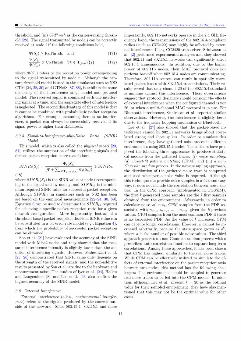
This model, which is also called the physical model [20,81], utilizes the summation of the interfering signals anddefines packet reception success as follows,
SINRi(Sj) = Ψi(Sj)(Ψ +
∑k∈Υj→i\j Ψi(Sk))
> SINRth
(18)where SINRi(Sj) is the SINR value at node i correspond-ing to the signal sent by node j, and SINRth is the mini-mum required SINR value for successful packet reception.Although SINRth in simulators such as NS2 has beenset based on the empirical measurements [22–24, 30, 89],Equation 6 can be used to determine the SINRth requiredfor achieving a specific packet reception ratio for a givennetwork configuration. More importantly, instead of athreshold-based packet reception decision, SINR value canbe substituted in a bit error rate model (e.g., Equation 4),from which the probability of successful packet receptioncan be obtained.
Son et al. [21] have evaluated the accuracy of the SINRmodel with Mica2 nodes and they showed that the mea-sured interference intensity is slightly lower than the ad-dition of interfering signals. However, Maheshwari et al.[25, 26] demonstrated that SINR value only depends onthe strength of the received signals, and the non-additiveresults presented by Son et al. are due to the hardware andmeasurement noise. The studies of Iyer et al. [24], Halkesand Langendoen [8], and Lee et al. [23] also confirm thehighest accuracy of the SINR model.
3.8. External InterferenceExternal interference (a.k.a., environmental interfer-
ence) refers to the signals produced by the sources out-side of the network. Since 802.15.4, 802.15.1 and more
importantly, 802.11b networks operate in the 2.4 GHz fre-quency band, the transmissions of the 802.15.4-compliantradios (such as CC2420) may highly be affected by exter-nal interference. Using CC2420 transceiver, Srinivasan etal. [2] performed experimental analyses and they showedthat 802.11 and 802.15.1 networks can significantly affect802.15.4 transmissions. In addition, due to the higherpower of 802.11b nodes, their MAC protocol does notperform backoff when 802.15.4 nodes are communicating.Therefore, 802.11b sources can result in spatially corre-lated packet losses with 802.15.4 transmissions. Their re-sults reveal that only channel 26 of the 802.15.4 standardis immune against this interference. These observationssuggest that protocol designers should consider the effectsof external interference when the configured channel is not26, or when a multi-channel MAC protocol is in use. ForBluetooth interference, Srinivasan et al. reported similarobservations. However, the interference is slightly lowerdue to the frequency hopping mechanism of Bluetooth.
Lee et al. [27] also showed that the packet-based in-terference caused by 802.11 networks brings about corre-lated strong and short spikes. In order to simulate thisinterference, they have gathered noise traces in differentenvironments using 802.15.4 nodes. The authors have pro-posed the following three approaches to produce statisti-cal models from the gathered traces: (i) naive sampling,(ii) closest-fit pattern matching (CPM), and (iii) a non-Gaussian random process. In the naive sampling approach,the distribution of the gathered noise trace is computedand used whenever a noise value is required. Althoughthis technique can provide noise samples in a fast and easyway, it does not include the correlation between noise val-ues. In the CPM approach (implemented in TOSSIM),the first k generated noise samples are the k first samplesobtained from the environment. Afterwards, in order tocalculate noise value nt, CPM samples from the PDF as-sociated with nt−1, nt−2, ... , nt−k, given the k previousvalues. CPM samples from the most common PDF if thereis no associated PDF. As the value of k increases, CPMcan capture longer correlations. However, k cannot be in-creased arbitrarily, because the state space grows as ak,where a is the number of possible noise values. The thirdapproach generates a non-Gaussian random process with aprescribed auto-correlation function to capture long-termcorrelations. Among these approaches, it has been shownthat CPM has highest similarity to the real noise traces.While CPM can be effectively utilized to simulate the ef-fects of external interference on the packet reception ratiobetween two nodes, this method has the following chal-lenges: The environment should be sampled to generatereal noise traces to be fed into the CPM model. In addi-tion, although Lee et al. present k = 20 as the optimalvalue for their sampled environment, they have also men-tioned that this may not be the optimal value for othercases.
11
B. Dezfouli et al. Journal of Network & Computer Applications (JNCA) | Elsevier
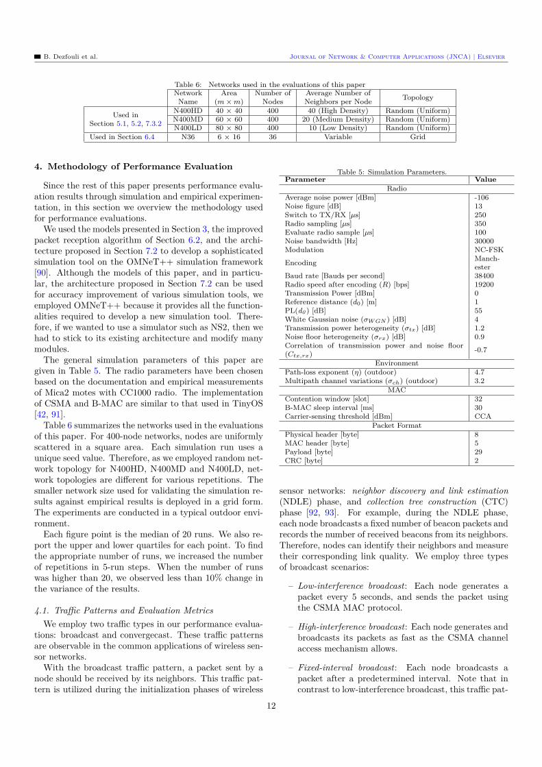
Table 6: Networks used in the evaluations of this paperNetwork
NameArea
(m × m)Number of
NodesAverage Number ofNeighbors per Node Topology
Used inSection 5.1, 5.2, 7.3.2
N400HD 40 × 40 400 40 (High Density) Random (Uniform)N400MD 60 × 60 400 20 (Medium Density) Random (Uniform)N400LD 80 × 80 400 10 (Low Density) Random (Uniform)
Used in Section 6.4 N36 6 × 16 36 Variable Grid
4. Methodology of Performance Evaluation
Since the rest of this paper presents performance evalu-ation results through simulation and empirical experimen-tation, in this section we overview the methodology usedfor performance evaluations.
We used the models presented in Section 3, the improvedpacket reception algorithm of Section 6.2, and the archi-tecture proposed in Section 7.2 to develop a sophisticatedsimulation tool on the OMNeT++ simulation framework[90]. Although the models of this paper, and in particu-lar, the architecture proposed in Section 7.2 can be usedfor accuracy improvement of various simulation tools, weemployed OMNeT++ because it provides all the function-alities required to develop a new simulation tool. There-fore, if we wanted to use a simulator such as NS2, then wehad to stick to its existing architecture and modify manymodules.
The general simulation parameters of this paper aregiven in Table 5. The radio parameters have been chosenbased on the documentation and empirical measurementsof Mica2 motes with CC1000 radio. The implementationof CSMA and B-MAC are similar to that used in TinyOS[42, 91].
Table 6 summarizes the networks used in the evaluationsof this paper. For 400-node networks, nodes are uniformlyscattered in a square area. Each simulation run uses aunique seed value. Therefore, as we employed random net-work topology for N400HD, N400MD and N400LD, net-work topologies are different for various repetitions. Thesmaller network size used for validating the simulation re-sults against empirical results is deployed in a grid form.The experiments are conducted in a typical outdoor envi-ronment.
Each figure point is the median of 20 runs. We also re-port the upper and lower quartiles for each point. To findthe appropriate number of runs, we increased the numberof repetitions in 5-run steps. When the number of runswas higher than 20, we observed less than 10% change inthe variance of the results.
4.1. Traffic Patterns and Evaluation MetricsWe employ two traffic types in our performance evalua-
tions: broadcast and convergecast. These traffic patternsare observable in the common applications of wireless sen-sor networks.
With the broadcast traffic pattern, a packet sent by anode should be received by its neighbors. This traffic pat-tern is utilized during the initialization phases of wireless
Table 5: Simulation Parameters.Parameter Value
RadioAverage noise power [dBm] -106Noise figure [dB] 13Switch to TX/RX [µs] 250Radio sampling [µs] 350Evaluate radio sample [µs] 100Noise bandwidth [Hz] 30000Modulation NC-FSK
Encoding Manch-ester
Baud rate [Bauds per second] 38400Radio speed after encoding (R) [bps] 19200Transmission Power [dBm] 0Reference distance (d0) [m] 1PL(d0 ) [dB] 55White Gaussian noise (σW GN ) [dB] 4Transmission power heterogeneity (σtx) [dB] 1.2Noise floor heterogeneity (σrx) [dB] 0.9Correlation of transmission power and noise floor(Ctx,rx) -0.7
EnvironmentPath-loss exponent (η) (outdoor) 4.7Multipath channel variations (σch) (outdoor) 3.2
MACContention window [slot] 32B-MAC sleep interval [ms] 30Carrier-sensing threshold [dBm] CCA
Packet FormatPhysical header [byte] 8MAC header [byte] 5Payload [byte] 29CRC [byte] 2
sensor networks: neighbor discovery and link estimation(NDLE) phase, and collection tree construction (CTC)phase [92, 93]. For example, during the NDLE phase,each node broadcasts a fixed number of beacon packets andrecords the number of received beacons from its neighbors.Therefore, nodes can identify their neighbors and measuretheir corresponding link quality. We employ three typesof broadcast scenarios:
– Low-interference broadcast: Each node generates apacket every 5 seconds, and sends the packet usingthe CSMA MAC protocol.
– High-interference broadcast: Each node generates andbroadcasts its packets as fast as the CSMA channelaccess mechanism allows.
– Fixed-interval broadcast: Each node broadcasts apacket after a predetermined interval. Note that incontrast to low-interference broadcast, this traffic pat-
12
B. Dezfouli et al. Journal of Network & Computer Applications (JNCA) | Elsevier
tern does not employ CSMA.
In all the broadcast traffic scenarios each node sends 50packets. Using the broadcast traffic pattern, we measurethe following metrics:
– Effective throughput: Indicates the total number ofcorrectly received packets at the nodes per second.
– Number of hidden-node collisions: A hidden-node col-lision happens when the radio is synchronized with anincoming signal, but a newly arrived signal corruptsthe first signal.
– RMSE : Indicates NDLE accuracy, which is repre-sented as RMSE =
√(∑N
i=1(li − ei)2)/N , where N
is the number of links, li is the average quality of linki, and ei is the estimated quality of link i.
– Number of discovered neighbors: The average numberof discovered neighbors per node.
– Receptions: Indicates the number of packets success-fully received by the nodes.
The most well-known application of sensor networks isto send their sensed data towards a common sink node[94, 95]. This many-to-one traffic pattern is referred to asconvergecast. Since the energy efficiency of this phase iscritical, B-MAC [42] is used as the MAC protocol. In ad-dition, evaluations with this traffic pattern are conductedwith the 400-node networks. We employ two types of con-vergecast scenarios:
– Low-interference convergecast: Each of the 20 nodesat the farthest distance from the sink node generatea packet every 5 minutes. Note that the sink node islocated at the top left corner of the network.
– High-interference convergecast: Each node generatesa packet every 30 seconds.
The following metrics are evaluated with the converge-cast traffic pattern:
– Packet delivery ratio: The ratio of the received pack-ets at sink to the total number of generated packets.
– Average end-to-end delay: The average packet delayfrom packet generation until reception at sink.
– Average number of hops: The average number of hopstraversed by the packets to reach the sink node.
Notice that convergecast requires the nodes to be awareof their paths towards the sink. In this paper, we assumethat nodes have established a data gathering tree duringthe initialization phase using the Collection Tree Protocol(CTP) [96]. In addition, in order to eliminate the negativeeffects of NDLE accuracy on data gathering performance,we run a high-accuracy NDLE protocol before data gath-ering.
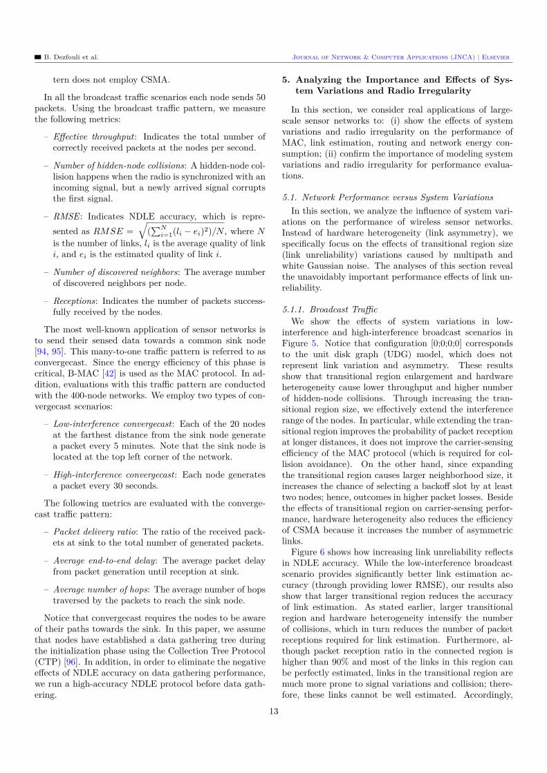
5. Analyzing the Importance and Effects of Sys-tem Variations and Radio Irregularity
In this section, we consider real applications of large-scale sensor networks to: (i) show the effects of systemvariations and radio irregularity on the performance ofMAC, link estimation, routing and network energy con-sumption; (ii) confirm the importance of modeling systemvariations and radio irregularity for performance evalua-tions.
5.1. Network Performance versus System VariationsIn this section, we analyze the influence of system vari-
ations on the performance of wireless sensor networks.Instead of hardware heterogeneity (link asymmetry), wespecifically focus on the effects of transitional region size(link unreliability) variations caused by multipath andwhite Gaussian noise. The analyses of this section revealthe unavoidably important performance effects of link un-reliability.
5.1.1. Broadcast TrafficWe show the effects of system variations in low-
interference and high-interference broadcast scenarios inFigure 5. Notice that configuration [0;0;0;0] correspondsto the unit disk graph (UDG) model, which does notrepresent link variation and asymmetry. These resultsshow that transitional region enlargement and hardwareheterogeneity cause lower throughput and higher numberof hidden-node collisions. Through increasing the tran-sitional region size, we effectively extend the interferencerange of the nodes. In particular, while extending the tran-sitional region improves the probability of packet receptionat longer distances, it does not improve the carrier-sensingefficiency of the MAC protocol (which is required for col-lision avoidance). On the other hand, since expandingthe transitional region causes larger neighborhood size, itincreases the chance of selecting a backoff slot by at leasttwo nodes; hence, outcomes in higher packet losses. Besidethe effects of transitional region on carrier-sensing perfor-mance, hardware heterogeneity also reduces the efficiencyof CSMA because it increases the number of asymmetriclinks.
Figure 6 shows how increasing link unreliability reflectsin NDLE accuracy. While the low-interference broadcastscenario provides significantly better link estimation ac-curacy (through providing lower RMSE), our results alsoshow that larger transitional region reduces the accuracyof link estimation. As stated earlier, larger transitionalregion and hardware heterogeneity intensify the numberof collisions, which in turn reduces the number of packetreceptions required for link estimation. Furthermore, al-though packet reception ratio in the connected region ishigher than 90% and most of the links in this region canbe perfectly estimated, links in the transitional region aremuch more prone to signal variations and collision; there-fore, these links cannot be well estimated. Accordingly,
13
B. Dezfouli et al. Journal of Network & Computer Applications (JNCA) | Elsevier
[0;0;0;0] [2;4;1.2;0.9] [4;4;1.2;0.9] [6;4;1.2;0.9]1
2
3
4
5
6
7x 10
5
Effec
tive
Thro
ughput
[Pack
et/S
econd](L
owIn
terf
eren
ce)
System Variations [σch; σW GN; σtx; σrx](a)
Broadcast
0.5
1
1.5
2
2.5
3
3.5x 10
5
Effec
tive
Thro
ughput
[Pac
ket
/Sec
ond](H
igh
Inte
rfer
ence
)
[0;0;0;0] [2;4;1.2;0.9] [4;4;1.2;0.9] [6;4;1.2;0.9]0
1
2
3
4
5
6
7x 10
4
Num
ber
ofH
idden
Node
Col
lisi
ons
(Low
Inte
rfer
ence
)
System Variations [σch; σW GN; σtx; σrx](b)
Broadcast
0.4
0.6
0.8
1
1.2
1.4
1.6
1.8
2
2.2x 10
5
Num
ber
ofH
idden
Node
Col
lisi
ons
(Hig
hIn
terf
eren
ce)
N400HD, Low Interference
N400MD, Low Interference
N400LD, Low Interference
N400HD, High Interference
N400MD, High Interference
N400LD, High Interference
Figure 5: Effects of system variations on the performance of packet broadcast. (a): Effective throughput; (b): Number of hidden-nodecollisions. Increasing the system variations generates more number of unreliable links, increases the interference distance, reduces theefficiency of carrier sensing, and results in higher packet corruptions.
[0;0;0;0] [2;4;1.2;0.9] [4;4;1.2;0.9] [6;4;1.2;0.9]0
0.1
0.2
0.3
0.4
0.5
0.6
0.7
0.8
0.9
1
RM
SE
(Low
Inte
rfer
ence
)
System Variations [σch; σW GN; σtx; σrx](a)
Broadcast
0
0.1
0.2
0.3
0.4
0.5
0.6
0.7
0.8
0.9
1
RM
SE
(Hig
hIn
terf
eren
ce)
[0;0;0;0] [2;4;1.2;0.9] [4;4;1.2;0.9] [6;4;1.2;0.9]10
15
20
25
30
35
40
45
50
55
Num
ber
ofD
isco
ver
edN
eigh
bors
/N
ode
(Low
Inte
rfer
ence
)
System Variations [σch; σW GN; σtx; σrx](b)
Broadcast
10
15
20
25
30
35
40
Num
ber
ofD
isco
ver
edN
eigh
bor
s/
Node
(Hig
hIn
terf
eren
ce)
N400HD, Low Interference
N400MD, Low Interference
N400LD, Low Interference
N400HD, High Interference
N400MD, High Interference
N400LD, High Interference
Figure 6: Effects of system variations on the accuracy of NDLE. (a): Link estimation accuracy (RMSE); (b): Average number of discoveredneighbors per node. While system variations highly affect NDLE performance, these effects specifically reflect in the performance of routingprotocols.
increasing system variations reduces link estimation ac-curacy, because it enlarges the ratio of the links in thetransitional region to those links in the connected region(cf. Section 3.1, Figure 2). Since most of the routing pro-tocols rely on link estimation [97, 98], these results revealthe potential influence of system variations on the perfor-mance of routing protocols.
As stated earlier, although enlarging the transitional re-gion improves the chance of packet reception at longerdistances, it also causes higher collision intensity and re-duces the chance of packet reception from neighbors. How-ever, due to the lower number of collisions in the low-interference scenario, the influence of larger transitionalregion on this scenario is the higher number of discoveredneighbors.
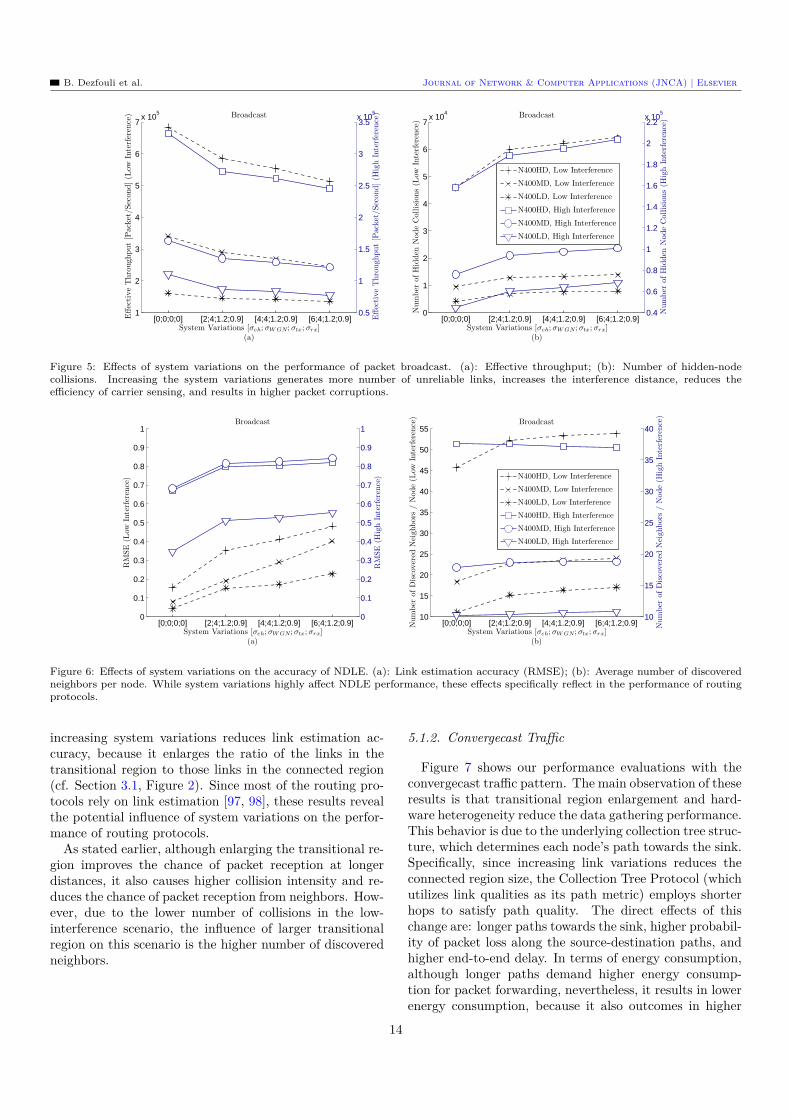
5.1.2. Convergecast Traffic
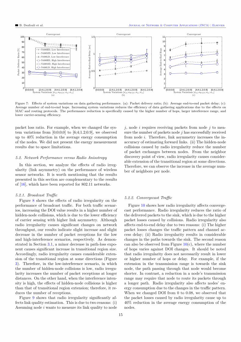
Figure 7 shows our performance evaluations with theconvergecast traffic pattern. The main observation of theseresults is that transitional region enlargement and hard-ware heterogeneity reduce the data gathering performance.This behavior is due to the underlying collection tree struc-ture, which determines each node’s path towards the sink.Specifically, since increasing link variations reduces theconnected region size, the Collection Tree Protocol (whichutilizes link qualities as its path metric) employs shorterhops to satisfy path quality. The direct effects of thischange are: longer paths towards the sink, higher probabil-ity of packet loss along the source-destination paths, andhigher end-to-end delay. In terms of energy consumption,although longer paths demand higher energy consump-tion for packet forwarding, nevertheless, it results in lowerenergy consumption, because it also outcomes in higher
14
B. Dezfouli et al. Journal of Network & Computer Applications (JNCA) | Elsevier
[0;0;0;0] [2;4;1.2;0.9] [4;4;1.2;0.9] [6;4;1.2;0.9]0
10
20
30
40
50
60
70
80
90
100
Pack
etD
eliv
ery
Rati
o[%
]
System Variations [σch; σWGN ; σtx; σrx](a)
Convergecast
N400HD, Low Interference
N400MD, Low Interference
N400LD, Low Interference
N400HD, High Interference
N400MD, High Interference
N400LD, High Interference
[0;0;0;0] [2;4;1.2;0.9] [4;4;1.2;0.9] [6;4;1.2;0.9]0
0.5
1
1.5
Aver
age
End-t
o-E
nd
Del
ay[s
ec]
System Variations [σch; σWGN ; σtx; σrx](b)
Convergecast
[0;0;0;0] [2;4;1.2;0.9] [4;4;1.2;0.9] [6;4;1.2;0.9]0
1
2
3
4
5
6
7
8
9
10
11
Aver
age
End-t
o-E
nd
Hops
System Variations [σch; σWGN ; σtx; σrx](c)
Convergecast
Figure 7: Effects of system variations on data gathering performance. (a): Packet delivery ratio; (b): Average end-to-end packet delay; (c):Average number of end-to-end hops. Increasing system variations reduces the efficiency of data gathering applications due to the effects onMAC and routing protocols. The performance reduction is specifically caused by the higher number of hops, larger interference range, andlower carrier-sensing efficiency.
packet loss ratio. For example, when we changed the sys-tem variations from [0;0;0;0] to [6;4;1.2;0.9], we observedup to 40% reduction in the average energy consumptionof the nodes. We did not present the energy measurementresults due to space limitations.
5.2. Network Performance versus Radio Anisotropy
In this section, we analyze the effects of radio irreg-ularity (link asymmetry) on the performance of wirelesssensor networks. It is worth mentioning that the resultspresented in this section are complementary to the resultsof [16], which have been reported for 802.11 networks.
5.2.1. Broadcast TrafficFigure 8 shows the effects of radio irregularity on the
performance of broadcast traffic. For both traffic scenar-ios, increasing the DOI value results in a higher number ofhidden-node collisions, which is due to the lower efficiencyof carrier sensing with higher link asymmetry. Althoughradio irregularity causes significant changes on networkthroughput, our results indicate slight increase and slightdecrease in the number of packet receptions for the lowand high-interference scenarios, respectively. As demon-strated in Section 3.1, a minor decrease in path-loss expo-nent causes significant increase in transitional region size.Accordingly, radio irregularity causes considerable exten-sion of the transitional region at some directions (Figure3). Therefore, in the low-interference scenario, in whichthe number of hidden-node collisions is low, radio irregu-larity increases the number of packet receptions at longerdistances. On the other hand, when the interference inten-sity is high, the effects of hidden-node collisions is higherthan that of transitional region extension; therefore, it re-duces the number of receptions.
Figure 9 shows that radio irregularity significantly af-fects link quality estimation. This is due to two reasons: (i)Assuming node i wants to measure its link quality to node
j, node i requires receiving packets from node j to mea-sure the number of packets node j has successfully receivedfrom node i. Therefore, link asymmetry increases the in-accuracy of estimating forward links. (ii) The hidden-nodecollisions caused by radio irregularity reduce the numberof packet exchanges between nodes. From the neighbordiscovery point of view, radio irregularity causes consider-able extension of the transitional region at some directions.Therefore, we can observe the increase in the average num-ber of neighbors per node.
5.2.2. Convergecast Traffic
Figure 10 shows how radio irregularity affects converge-cast performance. Radio irregularity reduces the ratio ofthe delivered packets to the sink, which is due to the higherpacket losses caused by collisions. Radio irregularity alsoaffects end-to-end delay due to two reasons: (i) The higherpacket losses changes the traffic pattern and channel ac-cess delay; (ii) Radio irregularity results in considerablechanges in the paths towards the sink. The second reasoncan also be observed from Figure 10(c), where the numberof hops varies against DOI changes. It should be notedthat radio irregularity does not necessarily result in loweror higher number of hops or delay. For example, if theextension in the transmission range is towards the sinknode, the path passing through that node would becomeshorter. In contrast, a reduction in a node’s transmissionrange may require that node to route its packets througha longer path. Radio irregularity also affects nodes’ en-ergy consumption due to the changes in the traffic pattern.When we changed DOI from 0 to 0.08, we observed thatthe packet losses caused by radio irregularity cause up to40% reduction in the average energy consumption of thenodes.
15
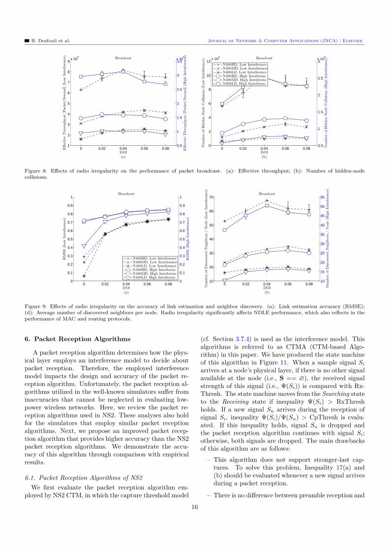
B. Dezfouli et al. Journal of Network & Computer Applications (JNCA) | Elsevier
0 0.02 0.04 0.06 0.081
2
3
4
5
6
7
8
9x 10
5
Effec
tive
Thro
ughput
[Pack
et/Sec
ond](L
ow
Inte
rfer
ence
)
DOI(a)
Broadcast
0.5
1
1.5
2
2.5
3
3.5x 10
5
Effec
tive
Thro
ughput
[Pack
et/Sec
ond](H
igh
Inte
rfer
ence
)
0 0.02 0.04 0.06 0.080
2
4
6
8
10
12x 10
4
Num
ber
ofH
idden
Node
Collisio
ns
(Low
Inte
rfer
ence
)
DOI(b)
Broadcast
0.5
1
1.5
2
2.5
3x 10
5
Num
ber
ofH
idden
Node
Collisio
ns
(Hig
hIn
terf
eren
ce)
N400HD, Low InterferenceN400MD, Low InterferenceN400LD, Low InterferenceN400HD, High InterferencN400MD, High InterferencN400LD, High Interferenc
Figure 8: Effects of radio irregularity on the performance of packet broadcast. (a): Effective throughput; (b): Number of hidden-nodecollisions.
0 0.02 0.04 0.06 0.080
0.1
0.2
0.3
0.4
0.5
0.6
0.7
0.8
0.9
1
DOI(a)
RM
SE
(Low
Inte
rfer
ence
)
Broadcast
0
0.1
0.2
0.3
0.4
0.5
0.6
0.7
0.8
0.9
1
RM
SE
(Hig
hIn
terf
eren
ce)
N400HD, Low InterferenceN400MD, Low InterferenceN400LD, Low InterferenceN400HD, High InterferencN400MD, High InterferencN400LD, High Interferenc
0 0.02 0.04 0.06 0.0810
20
30
40
50
60
70
Num
ber
ofD
isco
ver
edN
eighbors
/N
ode
(Low
Inte
rfer
ence
)
DOI(b)
Broadcast
10
15
20
25
30
35
40
45
50
55
Num
ber
ofD
isco
ver
edN
eighbors
/N
ode
(Hig
hIn
terf
eren
ce)
Figure 9: Effects of radio irregularity on the accuracy of link estimation and neighbor discovery. (a): Link estimation accuracy (RMSE);(d): Average number of discovered neighbors per node. Radio irregularity significantly affects NDLE performance, which also reflects in theperformance of MAC and routing protocols.
6. Packet Reception Algorithms
A packet reception algorithm determines how the phys-ical layer employs an interference model to decide aboutpacket reception. Therefore, the employed interferencemodel impacts the design and accuracy of the packet re-ception algorithm. Unfortunately, the packet reception al-gorithms utilized in the well-known simulators suffer frominaccuracies that cannot be neglected in evaluating low-power wireless networks. Here, we review the packet re-ception algorithms used in NS2. These analyses also holdfor the simulators that employ similar packet receptionalgorithms. Next, we propose an improved packet recep-tion algorithm that provides higher accuracy than the NS2packet reception algorithms. We demonstrate the accu-racy of this algorithm through comparison with empiricalresults.
6.1. Packet Reception Algorithms of NS2We first evaluate the packet reception algorithm em-
ployed by NS2 CTM, in which the capture threshold model
(cf. Section 3.7.4) is used as the interference model. Thisalgorithms is referred to as CTMA (CTM-based Algo-rithm) in this paper. We have produced the state machineof this algorithm in Figure 11. When a sample signal Si
arrives at a node’s physical layer, if there is no other signalavailable at the node (i.e., S == ∅), the received signalstrength of this signal (i.e., Ψ(Si)) is compared with Rx-Thresh. The state machine moves from the Searching stateto the Receiving state if inequality Ψ(Si) > RxThreshholds. If a new signal Sn arrives during the reception ofsignal Si, inequality Ψ(Si)/Ψ(Sn) > CpThresh is evalu-ated. If this inequality holds, signal Sn is dropped andthe packet reception algorithm continues with signal Si;otherwise, both signals are dropped. The main drawbacksof this algorithm are as follows:
– This algorithm does not support stronger-last cap-tures. To solve this problem, Inequality 17(a) and(b) should be evaluated whenever a new signal arrivesduring a packet reception.
– There is no difference between preamble reception and
16
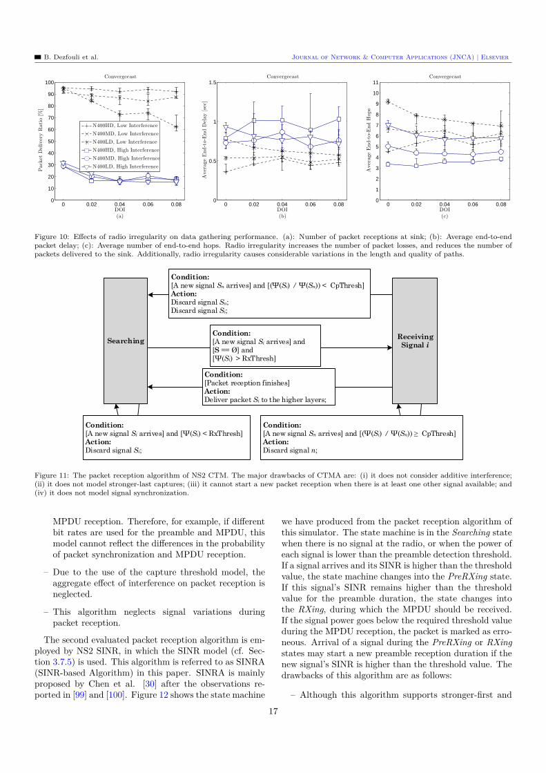
B. Dezfouli et al. Journal of Network & Computer Applications (JNCA) | Elsevier
0 0.02 0.04 0.06 0.080
10
20
30
40
50
60
70
80
90
100
Pack
etD
eliv
ery
Rati
o[%
]
DOI(a)
Convergecast
N400HD, Low Interference
N400MD, Low Interference
N400LD, Low Interference
N400HD, High Interference
N400MD, High Interference
N400LD, High Interference
0 0.02 0.04 0.06 0.080
0.5
1
1.5
Aver
age
End-t
o-E
nd
Del
ay[s
ec]
DOI(b)
Convergecast
0 0.02 0.04 0.06 0.080
1
2
3
4
5
6
7
8
9
10
11
Aver
age
End-t
o-E
nd
Hops
DOI(c)
Convergecast
Figure 10: Effects of radio irregularity on data gathering performance. (a): Number of packet receptions at sink; (b): Average end-to-endpacket delay; (c): Average number of end-to-end hops. Radio irregularity increases the number of packet losses, and reduces the number ofpackets delivered to the sink. Additionally, radio irregularity causes considerable variations in the length and quality of paths.
SearchingReceiving
Signal i
Condition:[A new signal Si arrives] and [Ψ(Si) < RxThresh]Action:Discard signal Si;
Condition:[A new signal Sn arrives] and [(Ψ(Si) / Ψ(Sn)) CpThresh]Action: Discard signal n;
Condition:[Packet reception finishes]Action:Deliver packet Si to the higher layers;
Condition:[A new signal Si arrives] and [S == Ø] and[Ψ(Si) > RxThresh]
Condition:[A new signal Sn arrives] and [(Ψ(Si) / Ψ(Sn)) < CpThresh]Action: Discard signal Sn;Discard signal Si;
Figure 11: The packet reception algorithm of NS2 CTM. The major drawbacks of CTMA are: (i) it does not consider additive interference;(ii) it does not model stronger-last captures; (iii) it cannot start a new packet reception when there is at least one other signal available; and(iv) it does not model signal synchronization.
MPDU reception. Therefore, for example, if differentbit rates are used for the preamble and MPDU, thismodel cannot reflect the differences in the probabilityof packet synchronization and MPDU reception.
– Due to the use of the capture threshold model, theaggregate effect of interference on packet reception isneglected.
– This algorithm neglects signal variations duringpacket reception.
The second evaluated packet reception algorithm is em-ployed by NS2 SINR, in which the SINR model (cf. Sec-tion 3.7.5) is used. This algorithm is referred to as SINRA(SINR-based Algorithm) in this paper. SINRA is mainlyproposed by Chen et al. [30] after the observations re-ported in [99] and [100]. Figure 12 shows the state machine
we have produced from the packet reception algorithm ofthis simulator. The state machine is in the Searching statewhen there is no signal at the radio, or when the power ofeach signal is lower than the preamble detection threshold.If a signal arrives and its SINR is higher than the thresholdvalue, the state machine changes into the PreRXing state.If this signal’s SINR remains higher than the thresholdvalue for the preamble duration, the state changes intothe RXing, during which the MPDU should be received.If the signal power goes below the required threshold valueduring the MPDU reception, the packet is marked as erro-neous. Arrival of a signal during the PreRXing or RXingstates may start a new preamble reception duration if thenew signal’s SINR is higher than the threshold value. Thedrawbacks of this algorithm are as follows:
– Although this algorithm supports stronger-first and
17

B. Dezfouli et al. Journal of Network & Computer Applications (JNCA) | Elsevier
SearchingPreRXing for signal PRX
RXing signal RX
Condition:[A new signal Si arrives] and [SINR(Si) < SINRth]Action:Discard signal Si;
Condition:[A new signal Si arrives] and [SINR(Si) SINRth]Action:PRX=Si;
Condition:[A new signal Sn arrives] and [SINR(PRX) < SINRth] and [SINR(Sn) < SINRth]Action: Discard signal PRX;Discard signal Sn;
Condition:[Successful PreRX for signal PRX]Action:RX = PRX;
Condition:[Receiving packet RX is finished]Action:Deliver packet Si to the higher layers;
Condition:[A new signal Sn arrives] and [SINR(RX) < SINRth] and [SINR(Sn) SINRth]Action: Discard signal RX;PRX = Sn;
Condition:[A new signal Sn arrives] and [SINR(RX) < SINRth] and[SINR(Sn) < SINRth]Action: Discard signal RX;Discard signal Sn;
Condition:[A new signal Sn arrives] and [SINR(PRX) < SINRth] and [SINR(Sn) SINRth]Action: Discard signal PRX;PRX = Sn;
Figure 12: The packet reception algorithm of NS2 SINR. The major drawbacks of SINRA are: (i) it does not provide accurate signalsynchronization, because the main decision for packet reception is made at packet arrival; (ii) decision for packet reception is based on thethreshold value.
stronger-last captures, it goes into the PreRXing stateif a signal’s SINR value is higher than a certain thresh-old upon its arrival. Therefore, when the preamblesize is larger than the settling bits, a packet cannotbe received if it cannot provide enough SINR upon itsarrival but its SINR value is large enough during thesettling bits.
– Since SINR evaluations are performed at signal ar-rival times, signal variations during packet receptioncannot be precisely modeled. In particular, instead ofusing a probabilistic packet reception model, thresh-old SINR values have been defined to decide aboutpreamble and MPDU reception.
Unfortunately, the packet reception algorithm of NS3 isalso similar to that of SINRA. Specifically, even with theimprovements proposed by [34], the packet reception algo-rithm of NS3 cannot receive those packets with partiallycorrupted preamble.
6.2. An Improved Packet Reception AlgorithmIn this section we propose the Capture Aware Reception
Model (CARM) to overcome the inaccuracies of CTMAand SINRA. The state machine of this model is given inFigure 13. In contrast with SINRA in which decision forpacket reception is made upon signal arrival, CARM per-forms continuous SINR evaluations to check whether asignal can be synchronized with the radio. To this aim,CARM requires managing two lists of signals:
– PreSYNC Signals: This list includes those signals thathave not reached their settling bits. A signal in thislist can be synchronized with the radio if it providesenough SINR during the settling bits.
– SYNC/MPDU Signals: This list includes those sig-nals that their settling bits are being arrived or arefinished. A signal of this list can be in one of thefollowing states: (i) PreRXing: if its SINR value ishigher than SINRth during the settling bits; (ii) RX-ing: if it has been successfully synchronized with thetransceiver.
When the state machine is in the Searching state anda signal is being moved from the PreSYNC Signals listto the SYNC/MPDU Signals lists, CARM checks whetherthe SINR of this signal is high enough for synchroniza-tion. If yes, the state is changed to the PreRXing state,and CARM evaluates the correct reception of the settlingbits of this signal. To evaluate the synchronization cor-rectness, CARM samples the signal’s SINR values duringthe settling bits, and uses these values to compute the cor-rectness of receiving the settling bits. State machine goesinto the RXing state if the reception of settling bits hasbeen successful. When the state machine is in the RX-ing state, the receiving signal’s SINR value is sampled aslong as its SINR is higher than SINRth. SINRth is theminimum SINR value required for receiving one byte.
18
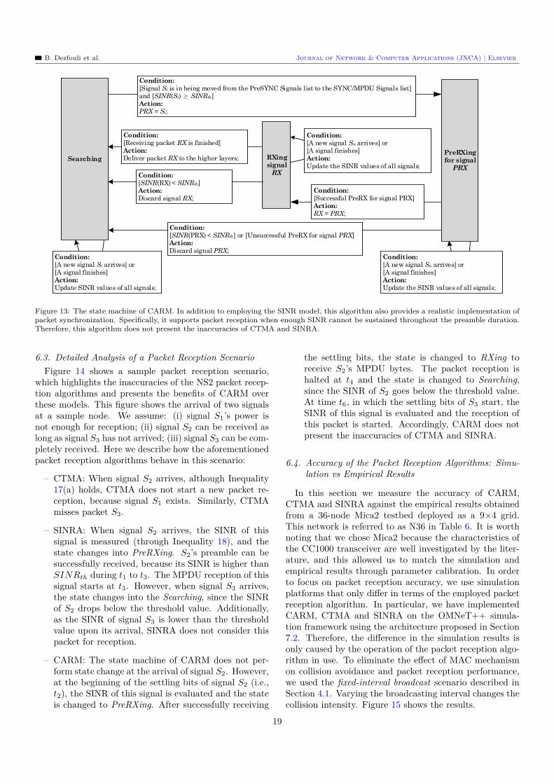
B. Dezfouli et al. Journal of Network & Computer Applications (JNCA) | Elsevier
SearchingPreRXing for signal PRX
RXing signal RX
Condition:[A new signal Si arrives] or [A signal finishes]Action:Update SINR values of all signals;
Condition:[Signal Si is in being moved from the PreSYNC Signals list to the SYNC/MPDU Signals list] and [SINR(Si) SINRth]Action:PRX = Si;
Condition:[Successful PreRX for signal PRX]Action:RX = PRX;
Condition:[Receiving packet RX is finished]Action: Deliver packet RX to the higher layers;
Condition:[A new signal Sn arrives] or [A signal finishes]Action: Update the SINR values of all signals;
Condition:[A new signal Sn arrives] or [A signal finishes]Action: Update the SINR values of all signals;
Condition:[SINR(RX) < SINRth]Action:Discard signal RX;
Condition:[SINR(PRX) < SINRth] or [Unsuccessful PreRX for signal PRX]Action:Discard signal PRX;
Figure 13: The state machine of CARM. In addition to employing the SINR model, this algorithm also provides a realistic implementation ofpacket synchronization. Specifically, it supports packet reception when enough SINR cannot be sustained throughout the preamble duration.Therefore, this algorithm does not present the inaccuracies of CTMA and SINRA.
6.3. Detailed Analysis of a Packet Reception ScenarioFigure 14 shows a sample packet reception scenario,
which highlights the inaccuracies of the NS2 packet recep-tion algorithms and presents the benefits of CARM overthese models. This figure shows the arrival of two signalsat a sample node. We assume: (i) signal S1’s power isnot enough for reception; (ii) signal S2 can be received aslong as signal S3 has not arrived; (iii) signal S3 can be com-pletely received. Here we describe how the aforementionedpacket reception algorithms behave in this scenario:
– CTMA: When signal S2 arrives, although Inequality17(a) holds, CTMA does not start a new packet re-ception, because signal S1 exists. Similarly, CTMAmisses packet S3.
– SINRA: When signal S2 arrives, the SINR of thissignal is measured (through Inequality 18), and thestate changes into PreRXing. S2’s preamble can besuccessfully received, because its SINR is higher thanSINRth during t1 to t3. The MPDU reception of thissignal starts at t3. However, when signal S3 arrives,the state changes into the Searching, since the SINRof S2 drops below the threshold value. Additionally,as the SINR of signal S3 is lower than the thresholdvalue upon its arrival, SINRA does not consider thispacket for reception.
– CARM: The state machine of CARM does not per-form state change at the arrival of signal S2. However,at the beginning of the settling bits of signal S2 (i.e.,t2), the SINR of this signal is evaluated and the stateis changed to PreRXing. After successfully receiving
the settling bits, the state is changed to RXing toreceive S2’s MPDU bytes. The packet reception ishalted at t4 and the state is changed to Searching,since the SINR of S2 goes below the threshold value.At time t6, in which the settling bits of S3 start, theSINR of this signal is evaluated and the reception ofthis packet is started. Accordingly, CARM does notpresent the inaccuracies of CTMA and SINRA.
6.4. Accuracy of the Packet Reception Algorithms: Simu-lation vs Empirical Results
In this section we measure the accuracy of CARM,CTMA and SINRA against the empirical results obtainedfrom a 36-node Mica2 testbed deployed as a 9×4 grid.This network is referred to as N36 in Table 6. It is worthnoting that we chose Mica2 because the characteristics ofthe CC1000 transceiver are well investigated by the liter-ature, and this allowed us to match the simulation andempirical results through parameter calibration. In orderto focus on packet reception accuracy, we use simulationplatforms that only differ in terms of the employed packetreception algorithm. In particular, we have implementedCARM, CTMA and SINRA on the OMNeT++ simula-tion framework using the architecture proposed in Section7.2. Therefore, the difference in the simulation results isonly caused by the operation of the packet reception algo-rithm in use. To eliminate the effect of MAC mechanismon collision avoidance and packet reception performance,we used the fixed-interval broadcast scenario described inSection 4.1. Varying the broadcasting interval changes thecollision intensity. Figure 15 shows the results.
19
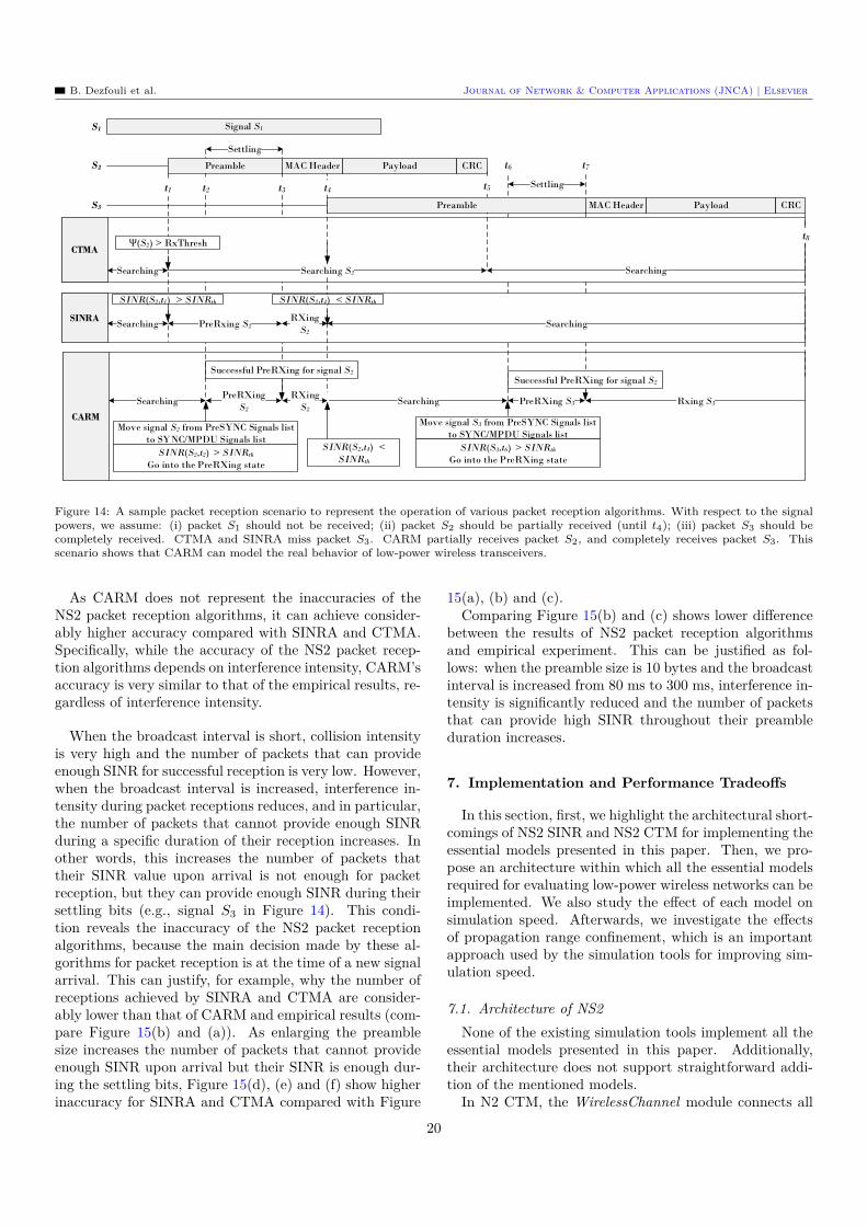
B. Dezfouli et al. Journal of Network & Computer Applications (JNCA) | Elsevier
S2
S3 CRCPreamble Payload
Settling
MAC Header
Searching S2
PreRxing S2 Searching
SINR(S2,t4) < SINRth
Searching PreRXing S3
Move signal S3 from PreSYNC Signals list
to SYNC/MPDU Signals list
SINR(S3,t6) > SINRth
Go into the PreRXing state
Rxing S3
t6 t7
t8
Successful PreRXing for signal S2
t2
CRCPreamble PayloadMAC Header
Signal S1S1
Ѱ(S2) > RxThresh
Searching
Searching
SINR(S2,t1) > SINRth
t1
RXing
S2
CTMA
SINRA
Settling
SearchingPreRXing
S2
Move signal S2 from PreSYNC Signals list
to SYNC/MPDU Signals list
SINR(S2,t2) > SINRth
Go into the PreRXing state
RXing
S2
Successful PreRXing for signal S2
SINR(S2,t4) <
SINRth
CARM
t3 t4 t5
Figure 14: A sample packet reception scenario to represent the operation of various packet reception algorithms. With respect to the signalpowers, we assume: (i) packet S1 should not be received; (ii) packet S2 should be partially received (until t4); (iii) packet S3 should becompletely received. CTMA and SINRA miss packet S3. CARM partially receives packet S2, and completely receives packet S3. Thisscenario shows that CARM can model the real behavior of low-power wireless transceivers.
As CARM does not represent the inaccuracies of theNS2 packet reception algorithms, it can achieve consider-ably higher accuracy compared with SINRA and CTMA.Specifically, while the accuracy of the NS2 packet recep-tion algorithms depends on interference intensity, CARM’saccuracy is very similar to that of the empirical results, re-gardless of interference intensity.
When the broadcast interval is short, collision intensityis very high and the number of packets that can provideenough SINR for successful reception is very low. However,when the broadcast interval is increased, interference in-tensity during packet receptions reduces, and in particular,the number of packets that cannot provide enough SINRduring a specific duration of their reception increases. Inother words, this increases the number of packets thattheir SINR value upon arrival is not enough for packetreception, but they can provide enough SINR during theirsettling bits (e.g., signal S3 in Figure 14). This condi-tion reveals the inaccuracy of the NS2 packet receptionalgorithms, because the main decision made by these al-gorithms for packet reception is at the time of a new signalarrival. This can justify, for example, why the number ofreceptions achieved by SINRA and CTMA are consider-ably lower than that of CARM and empirical results (com-pare Figure 15(b) and (a)). As enlarging the preamblesize increases the number of packets that cannot provideenough SINR upon arrival but their SINR is enough dur-ing the settling bits, Figure 15(d), (e) and (f) show higherinaccuracy for SINRA and CTMA compared with Figure
15(a), (b) and (c).Comparing Figure 15(b) and (c) shows lower difference
between the results of NS2 packet reception algorithmsand empirical experiment. This can be justified as fol-lows: when the preamble size is 10 bytes and the broadcastinterval is increased from 80 ms to 300 ms, interference in-tensity is significantly reduced and the number of packetsthat can provide high SINR throughout their preambleduration increases.
7. Implementation and Performance Tradeoffs
In this section, first, we highlight the architectural short-comings of NS2 SINR and NS2 CTM for implementing theessential models presented in this paper. Then, we pro-pose an architecture within which all the essential modelsrequired for evaluating low-power wireless networks can beimplemented. We also study the effect of each model onsimulation speed. Afterwards, we investigate the effectsof propagation range confinement, which is an importantapproach used by the simulation tools for improving sim-ulation speed.
7.1. Architecture of NS2None of the existing simulation tools implement all the
essential models presented in this paper. Additionally,their architecture does not support straightforward addi-tion of the mentioned models.
In N2 CTM, the WirelessChannel module connects all
20
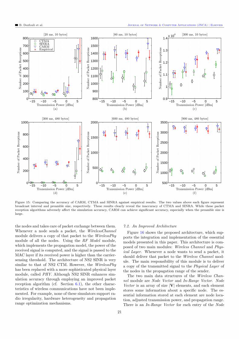
B. Dezfouli et al. Journal of Network & Computer Applications (JNCA) | Elsevier
Transmission Power [dBm](a)
Num
ber
ofP
ack
etR
ecep
tions
[20 ms, 10 bytes]
−15 −10 −5 0 50
100
200
300
400
500
600
700
800CTMASINRACARMEmpirical
Transmission Power [dBm](b)
Num
ber
ofP
ack
etR
ecep
tions
[80 ms, 10 bytes]
−15 −10 −5 0 5800
900
1000
1100
1200
1300
1400
1500
1600
Transmission Power [dBm](c)
Num
ber
ofP
ack
etR
ecep
tions
[300 ms, 10 bytes]
−15 −10 −5 0 50.9
1
1.1
1.2
1.3
1.4x 10
4
Transmission Power [dBm](d)
Num
ber
ofP
ack
etR
ecep
tions
[300 ms, 480 bytes]
−15 −10 −5 0 50
200
400
600
800
1000
Transmission Power [dBm](e)
Num
ber
ofP
ack
etR
ecep
tions
[600 ms, 480 bytes]
−15 −10 −5 0 50
500
1000
1500
2000
Transmission Power [dBm](f)
Num
ber
ofP
ack
etR
ecep
tions
[900 ms, 480 bytes]
−15 −10 −5 0 5500
1000
1500
2000
2500
3000
3500
Figure 15: Comparing the accuracy of CARM, CTMA and SINRA against empirical results. The two values above each figure representbroadcast interval and preamble size, respectively. These results clearly reveal the inaccuracy of CTMA and SINRA. While these packetreception algorithms adversely affect the simulation accuracy, CARM can achieve significant accuracy, especially when the preamble size islarge.
the nodes and takes care of packet exchange between them.Whenever a node sends a packet, the WirelessChannelmodule delivers a copy of that packet to the WirelessPhymodule of all the nodes. Using the RF Model module,which implements the propagation model, the power of thereceived signal is computed, and the signal is passed to theMAC layer if its received power is higher than the carrier-sensing threshold. The architecture of NS2 SINR is verysimilar to that of NS2 CTM. However, the WirelessPhyhas been replaced with a more sophisticated physical layermodule, called PHY. Although NS2 SINR enhances sim-ulation accuracy through employing an improved packetreception algorithm (cf. Section 6.1), the other charac-teristics of wireless communications have not been imple-mented. For example, none of these simulators support ra-dio irregularity, hardware heterogeneity and propagationrange optimization mechanisms.
7.2. An Improved ArchitectureFigure 16 shows the proposed architecture, which sup-
ports the integration and implementation of the essentialmodels presented in this paper. This architecture is com-posed of two main modules: Wireless Channel and Phys-ical Layer. Whenever a node wants to send a packet, itshould deliver that packet to the Wireless Channel mod-ule. The main responsibility of this module is to delivera copy of the transmitted signal to the Physical Layer ofthe nodes in the propagation range of the sender.
The two main data structures of the Wireless Chan-nel module are Node Vector and In-Range Vector. NodeVector is an array of size |V| elements, and each elementstores some information about a specific node. The es-sential information stored at each element are node loca-tion, adjusted transmission power, and propagation range.There is an In-Range Vector for each entry of the Node
21
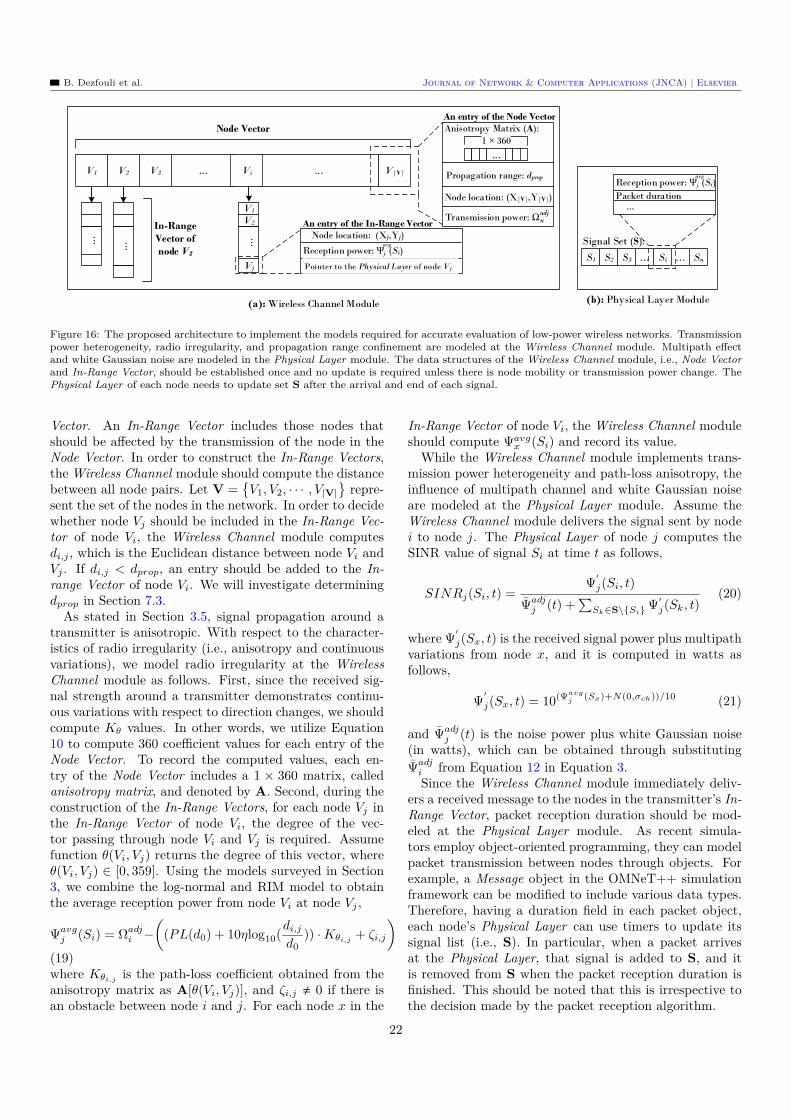
B. Dezfouli et al. Journal of Network & Computer Applications (JNCA) | Elsevier
V1 V2 V3 ... V|V|
Node Vector
...
In-Range
Vector of
node V2
...Vi
...
...
1 × 360
Anisotropy Matrix (A):
Node location: (X|V|,Y|V|)
Node location: (Xj,Yj)
An entry of the Node Vector
An entry of the In-Range Vector
V1
V2
Vj
...
(a): Wireless Channel Module (b): Physical Layer Module
Transmission power: adjn
S1 S2 S3 ... Si ... Sn
Signal Set (S):
Pointer to the Physical Layer of node Vj
Packet duration...
Propagation range: dprop
jReception power: Ψ (Si)avg
jReception power: Ψ (Si)avg
Figure 16: The proposed architecture to implement the models required for accurate evaluation of low-power wireless networks. Transmissionpower heterogeneity, radio irregularity, and propagation range confinement are modeled at the Wireless Channel module. Multipath effectand white Gaussian noise are modeled in the Physical Layer module. The data structures of the Wireless Channel module, i.e., Node Vectorand In-Range Vector, should be established once and no update is required unless there is node mobility or transmission power change. ThePhysical Layer of each node needs to update set S after the arrival and end of each signal.
Vector. An In-Range Vector includes those nodes thatshould be affected by the transmission of the node in theNode Vector. In order to construct the In-Range Vectors,the Wireless Channel module should compute the distancebetween all node pairs. Let V =
V1, V2, · · · , V|V|
repre-
sent the set of the nodes in the network. In order to decidewhether node Vj should be included in the In-Range Vec-tor of node Vi, the Wireless Channel module computesdi,j , which is the Euclidean distance between node Vi andVj . If di,j < dprop, an entry should be added to the In-range Vector of node Vi. We will investigate determiningdprop in Section 7.3.
As stated in Section 3.5, signal propagation around atransmitter is anisotropic. With respect to the character-istics of radio irregularity (i.e., anisotropy and continuousvariations), we model radio irregularity at the WirelessChannel module as follows. First, since the received sig-nal strength around a transmitter demonstrates continu-ous variations with respect to direction changes, we shouldcompute Kθ values. In other words, we utilize Equation10 to compute 360 coefficient values for each entry of theNode Vector. To record the computed values, each en-try of the Node Vector includes a 1 × 360 matrix, calledanisotropy matrix, and denoted by A. Second, during theconstruction of the In-Range Vectors, for each node Vj inthe In-Range Vector of node Vi, the degree of the vec-tor passing through node Vi and Vj is required. Assumefunction θ(Vi, Vj) returns the degree of this vector, whereθ(Vi, Vj) ∈ [0, 359]. Using the models surveyed in Section3, we combine the log-normal and RIM model to obtainthe average reception power from node Vi at node Vj ,
Ψavgj (Si) = Ωadj
i −(
(PL(d0) + 10ηlog10(di,j
d0)) · Kθi,j + ζi,j
)(19)where Kθi,j is the path-loss coefficient obtained from theanisotropy matrix as A[θ(Vi, Vj)], and ζi,j , 0 if there isan obstacle between node i and j. For each node x in the
In-Range Vector of node Vi, the Wireless Channel moduleshould compute Ψavg
x (Si) and record its value.While the Wireless Channel module implements trans-
mission power heterogeneity and path-loss anisotropy, theinfluence of multipath channel and white Gaussian noiseare modeled at the Physical Layer module. Assume theWireless Channel module delivers the signal sent by nodei to node j. The Physical Layer of node j computes theSINR value of signal Si at time t as follows,
SINRj(Si, t) =Ψ′
j(Si, t)Ψadj
j (t) +∑
Sk∈S\Si Ψ′j(Sk, t)
(20)
where Ψ′
j(Sx, t) is the received signal power plus multipathvariations from node x, and it is computed in watts asfollows,
Ψ′
j(Sx, t) = 10(Ψavgj
(Sx)+N(0,σch))/10 (21)
and Ψadjj (t) is the noise power plus white Gaussian noise
(in watts), which can be obtained through substitutingΨadj
i from Equation 12 in Equation 3.Since the Wireless Channel module immediately deliv-
ers a received message to the nodes in the transmitter’s In-Range Vector, packet reception duration should be mod-eled at the Physical Layer module. As recent simula-tors employ object-oriented programming, they can modelpacket transmission between nodes through objects. Forexample, a Message object in the OMNeT++ simulationframework can be modified to include various data types.Therefore, having a duration field in each packet object,each node’s Physical Layer can use timers to update itssignal list (i.e., S). In particular, when a packet arrivesat the Physical Layer, that signal is added to S, and itis removed from S when the packet reception duration isfinished. This should be noted that this is irrespective tothe decision made by the packet reception algorithm.
22
B. Dezfouli et al. Journal of Network & Computer Applications (JNCA) | Elsevier
The proposed architecture can be used for implementingvarious models in existing simulation tools. However, asmentioned in Section 4, we employed the OMNeT++ sim-ulation framework to develop the simulation tool used inthis paper, because this framework only provides the basisrequired to develop a new simulation tool. Therefore, wecould easily implement new modules, without eliminationor modifying any existing module.
When the relationship between packet transmission du-ration and mobility speed allows us to assume that thevariation of reception power during a packet receptionis negligible, node mobility can be modeled as follows:Whenever a node moves, it can notify the Wireless Chan-nel module about its new position. As a position changemay affect the signal level between nodes, the WirelessChannel module should update the In-Range Vectors. Theupdate cost is O(|V|2).
The proposed architecture can also be used for evaluat-ing transmission power control protocols. Although wire-less transceivers allow transmission power configuration,the transmission power is fixed for at least a packet trans-mission duration. Therefore, whenever the transmissionpower of a node changes, the In-Range Vector of that nodeshould be updated. The update cost is O(|V|).
7.2.1. Effect on Simulation SpeedThe aforementioned architecture includes various mod-
els with different computational demands. This sectionaims to discuss about the effects of these models on simu-lation speed.
– Hardware Heterogeneity: At simulation initialization,using a hardware heterogeneity model (cf. Section3.6) each node computes the deviation of its noisefloor and transmission power from the average com-puted values. Each node also informs the Wire-less Channel module about its adjusted transmis-sion power value. As these values are fixed for eachnode throughout a simulation experiment, they donot affect simulation speed. However, it should benoted that the transmission power increment causedby hardware heterogeneity may increase the effect ofa node’s transmission on other nodes. With respectto interference, increasing the interference range ofa node results in higher number of signal arrivals atother nodes, and this increases the number of compu-tations related to the packet reception algorithm. Fur-thermore, as increasing a node’s transmission powermay increase the number of neighbors that can receivethis node’s packet, the number of computations per-taining to packet reception algorithm intensifies. Sim-ilarly, since reducing a node’s noise floor may increasethe chance of packet reception, the computations per-taining to packet reception algorithm increases.
– Radio Irregularity: Similar to hardware heterogene-ity, the computations regarding radio irregularity are
only performed at simulation initialization and theydo not have any effect on simulation speed. However,as the increment or decrement of transmission poweraffect the signal relationship between nodes, radio ir-regularity may affect the computations pertaining topacket reception algorithm.
– Log-normal Shadowing Model: The fixed part of thismodel (i.e., PL(d0) + 10ηlog( d
d0)) has been imple-
mented in the Wireless Channel module (cf. Equa-tion 19), therefore it has no effect on simulation speed.However, as the variable part (i.e., N(0, σch)) is im-plemented within the SINR model (cf. Equation 20and 21), its overhead depends on the number of sig-nals arriving at each node and the number of packetsthat can be received by each node.
– Noise Floor Variations: As this model is implementedwithin the SINR model (cf. Equation 20), its overheaddepends on the number of signals arriving at eachnode and the number of packets that can be receivedby each node.
7.3. Propagation Range OptimizationThis section addresses simulation speed improvement
thorough propagation range confinement. Propagationrange considerably influences the simulation speed. Specif-ically, as long as there are some nodes that their propa-gation range does not cover the entire network, increas-ing the propagation range reduces the simulation speed,which is due to the increase in computational and mem-ory management costs. For example, each signal arrivalat a node triggers the packet reception algorithm to per-form some computations regarding the power of the newsignal or the SINR of the signal currently begin received.On the other hand, increasing the propagation range in-tensifies the number of generated events, which increasesthe memory management costs. For example, more num-ber of packet copies should be generated and delivered tothe nodes. This section, first, studies the existing prop-agation range confinement methods, then, the effects ofpropagation range confinement are evaluated in terms ofsimulation speed and accuracy.
7.3.1. Existing ApproachesWith respect to the considerable effects of propagation
range on simulation scalability [33, 35], most of the simula-tors confine the propagation range to improve the simula-tion speed. In Castalia, a transmitted signal is delivered toa node if the received signal power at the receiver is about10 dB lower than the noise floor. In GloMoSim, the areais divided into sub-areas, and a message transmitted by anode is only delivered to its neighboring sub-areas. GT-NetS defines an interference range for signal propagation.In NS2 CTM, the WirelessPhy module delivers a signal tothe MAC layer if its received signal power is higher thanthe carrier-sensing threshold.
23
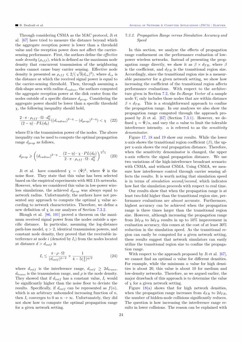
B. Dezfouli et al. Journal of Network & Computer Applications (JNCA) | Elsevier
Through considering CSMA as the MAC protocol, Ji etal. [67] have tried to measure the distance beyond whichthe aggregate reception power is lower than a thresholdvalue and the reception power does not affect the carrier-sensing performance. First, the authors define the effectivenode density (ρeff ), which is defined as the maximum nodedensity that concurrent transmission of the neighboringnodes cannot cause busy carrier sensing. Effective nodedensity is presented as ρeff 6 2/(
√3(dcs)2), where dcs is
the distance at which the received signal power is equal tothe carrier-sensing threshold. Then, through assuming adisk-shape area with radius dradius, the authors computedthe aggregate reception power at the disk center from thenodes outside of a specific distance dprop. Considering theaggregate power should be lower than a specific thresholdχ, the following inequality should hold,
2 · π · ρeff · Ω · dη0
(2 − η) · PL(d0) ((dradius)2−η − (dprop)2−η) < χ (22)
where Ω is the transmission power of the nodes. The aboveinequality can be used to compute the optimal propagationrange dprop as follows,
dprop >
((dradius)2−η − (2 − η) · χ · PL(d0)
2 · π · ρeff · Ω · dη0
) 12−η
(23)
Ji et al. have considered χ = (Ψ)2, where Ψ is thenoise floor. They state that this value has been selectedbased on the empirical experiments with 802.11b networks.However, when we considered this value in low-power wire-less simulations, the achieved dprop was always equal tonetwork radius. Unfortunately, the authors have not pre-sented any approach to compute the optimal χ value ac-cording to network characteristics. Therefore, we define anew definition of χ in our analyses of Section 7.3.2.
Blough et al. [86, 101] proved a theorem on the maxi-mum received signal power from the nodes outside a spe-cific distance. In particular, assuming the log-distancepath-loss model, η > 2, identical transmission powers, andconstant node density, they proved that the receivable in-terference at node i (denoted by Ii) from the nodes locatedat distance d > dintf is
Ii ≤ π · ρ · Ω(dintf )η−2 × 1
4 − 5( 45 )η/2 (24)
where dintf is the interference range, dintf ≥ 2dtrans,dtrans is the transmission range, and ρ is the node density.They showed that if dintf has a constant value, Ii wouldbe significantly higher than the noise floor to deviate theresults. Specifically, if dintf can be represented as f(n),which is an arbitrary unbounded increasing function of n,then Ii converges to 0 as n → ∞. Unfortunately, they didnot show how to compute the optimal propagation rangefor a given network setting.
7.3.2. Propagation Range versus Simulation Accuracy andSpeed
In this section, we analyze the effects of propagationrange confinement on the performance evaluation of low-power wireless networks. Instead of presenting the prop-agation range directly, we show it as β × dT R, where βis the coefficient, and dT R is the transitional region size.Accordingly, since the transitional region size is a measur-able parameter for a given network setting, we show howincreasing the coefficient of the transitional region affectsperformance evaluations. With respect to the architec-ture given in Section 7.2, the In-Range Vector of a samplenode Vi only includes those nodes that are within distanceβ × dT R. This is a straightforward approach to confinethe propagation range. In our analyses we also show thepropagation range computed through the approach pro-posed by Ji et al. [67] (Section 7.3.1). However, we de-fined χ = Ψ/α, and vary the α value to limit the tolerableinterference intensity. α is referred to as the sensitivitydenominator.
Figure 17, 18 and 19 show our results. While the lowerx-axis shows the transitional region coefficient (β), the up-per x-axis shows the real propagation distance. Therefore,when the sensitivity denominator is changed, the upperx-axis reflects the signal propagation distance. We usetwo variations of the high-interference broadcast scenario:with CSMA, and without CSMA. Using CSMA, we mea-sure how interference control through carrier sensing af-fects the results. It is worth noting that simulation speedis in terms of simulation second/second, which indicateshow fast the simulation proceeds with respect to real time.
Our results show that when the propagation range is atleast two-fold higher than the transitional region size, per-formance evaluations are almost accurate. Furthermore,highest accuracy can be achieved when the propagationrange is three times larger than the transitional regionsize. However, although increasing the propagation rangefrom 2dT R to 3dT R results in up to 10% improvement inevaluation accuracy, this comes at the cost of at least 30%reduction in the simulation speed. As the transitional re-gion can easily be computed for a given network setting,these results suggest that network simulators can easilyutilize the transitional region size to confine the propaga-tion range.
With respect to the approach proposed by Ji et al. [67],we cannot find an optimal α value for different densities.For example, while the minimum α value for high densi-ties is about 20, this value is about 10 for medium andlow-density networks. Therefore, as we argued earlier, themajor drawback of this approach is to determine the valueof χ for a given network setting.
Figure 18(a) shows that for high network densities,when the propagation range increases from dT R to 2dT R,the number of hidden-node collisions significantly reduces.The question is how increasing the interference range re-sults in lower collisions. The reason can be explained with
24
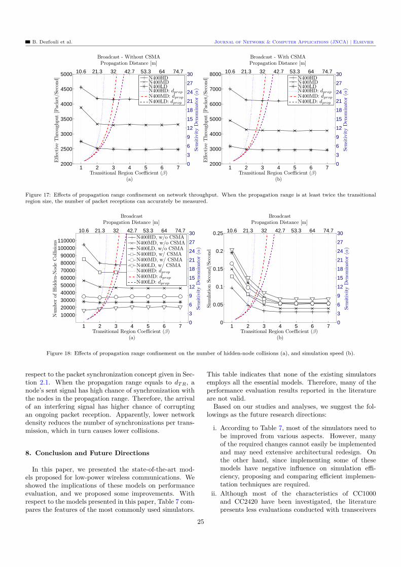
B. Dezfouli et al. Journal of Network & Computer Applications (JNCA) | Elsevier
1 2 3 4 5 6 72000
2500
3000
3500
4000
4500
5000
Effec
tive
Thro
ugh
put
[Pac
ket
/Sec
ond]
Transitional Region Coefficient (β)(a)
Broadcast - Without CSMAPropagation Distance [m]
10.6 21.3 32 42.7 53.3 64 74.7
0
3
6
9
12
15
18
21
24
27
30
Sen
sitivity
Den
omin
ator
(α)
N400HDN400MDN400LDN400HD: dprop
N400MD: dprop
N400LD: dprop
1 2 3 4 5 6 72000
3000
4000
5000
6000
7000
8000
Effec
tive
Thro
ugh
put
[Pac
ket
/Sec
ond]
Broadcast - With CSMAPropagation Distance [m]
Transitional Region Coefficient (β)(b)
10.6 21.3 32 42.7 53.3 64 74.7
0
3
6
9
12
15
18
21
24
27
30
Sen
sitivity
Den
omin
ator
(α)
N400HDN400MDN400LDN400HD: dprop
N400MD: dprop
N400LD: dprop
Figure 17: Effects of propagation range confinement on network throughput. When the propagation range is at least twice the transitionalregion size, the number of packet receptions can accurately be measured.
1 2 3 4 5 6 7
100002000030000400005000060000700008000090000
100000110000
Num
ber
ofH
idden
-Node
Col
lision
s
Transitional Region Coefficient (β)(a)
BroadcastPropagation Distance [m]
10.6 21.3 32 42.7 53.3 64 74.7
0
3
6
9
12
15
18
21
24
27
30
Sen
sitivity
Den
omin
ator
(α)
N400HD, w/o CSMAN400MD, w/o CSMAN400LD, w/o CSMAN400HD, w/ CSMAN400MD, w/ CSMAN400LD, w/ CSMAN400HD: dprop
N400MD: dprop
N400LD: dprop
1 2 3 4 5 6 70
0.05
0.1
0.15
0.2
0.25
Sim
ula
tion
Sec
ond/S
econ
d
Transitional Region Coefficient (β)(b)
BroadcastPropagation Distance [m]
10.6 21.3 32 42.7 53.3 64 74.7
0
3
6
9
12
15
18
21
24
27
30
Sen
sitivity
Den
omin
ator
(α)
Figure 18: Effects of propagation range confinement on the number of hidden-node collisions (a), and simulation speed (b).
respect to the packet synchronization concept given in Sec-tion 2.1. When the propagation range equals to dT R, anode’s sent signal has high chance of synchronization withthe nodes in the propagation range. Therefore, the arrivalof an interfering signal has higher chance of corruptingan ongoing packet reception. Apparently, lower networkdensity reduces the number of synchronizations per trans-mission, which in turn causes lower collisions.
8. Conclusion and Future Directions
In this paper, we presented the state-of-the-art mod-els proposed for low-power wireless communications. Weshowed the implications of these models on performanceevaluation, and we proposed some improvements. Withrespect to the models presented in this paper, Table 7 com-pares the features of the most commonly used simulators.
This table indicates that none of the existing simulatorsemploys all the essential models. Therefore, many of theperformance evaluation results reported in the literatureare not valid.
Based on our studies and analyses, we suggest the fol-lowings as the future research directions:
i. According to Table 7, most of the simulators need tobe improved from various aspects. However, manyof the required changes cannot easily be implementedand may need extensive architectural redesign. Onthe other hand, since implementing some of thesemodels have negative influence on simulation effi-ciency, proposing and comparing efficient implemen-tation techniques are required.
ii. Although most of the characteristics of CC1000and CC2420 have been investigated, the literaturepresents less evaluations conducted with transceivers
25
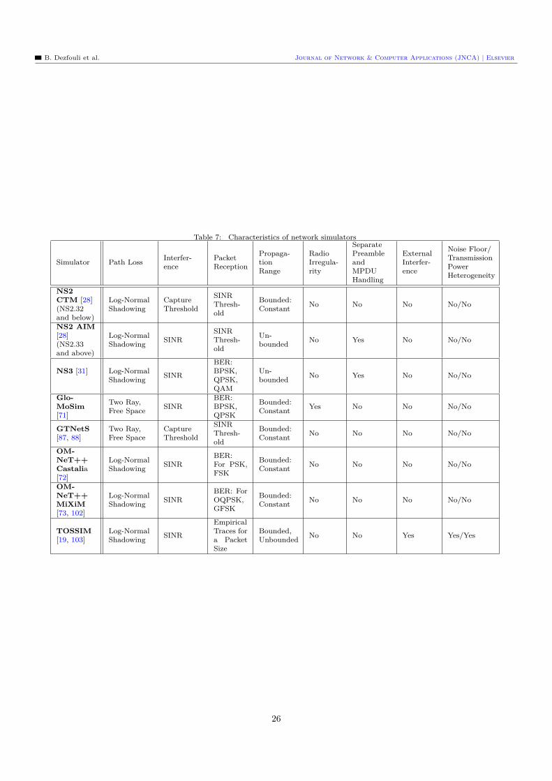
B. Dezfouli et al. Journal of Network & Computer Applications (JNCA) | Elsevier
Table 7: Characteristics of network simulators
Simulator Path Loss Interfer-ence
PacketReception
Propaga-tionRange
RadioIrregula-rity
SeparatePreambleandMPDUHandling
ExternalInterfer-ence
Noise Floor/TransmissionPowerHeterogeneity
NS2CTM [28](NS2.32and below)
Log-NormalShadowing
CaptureThreshold
SINRThresh-old
Bounded:Constant No No No No/No
NS2 AIM[28](NS2.33and above)
Log-NormalShadowing SINR
SINRThresh-old
Un-bounded No Yes No No/No
NS3 [31] Log-NormalShadowing SINR
BER:BPSK,QPSK,QAM
Un-bounded No Yes No No/No
Glo-MoSim[71]
Two Ray,Free Space SINR
BER:BPSK,QPSK
Bounded:Constant Yes No No No/No
GTNetS[87, 88]
Two Ray,Free Space
CaptureThreshold
SINRThresh-old
Bounded:Constant No No No No/No
OM-NeT++Castalia[72]
Log-NormalShadowing SINR
BER:For PSK,FSK
Bounded:Constant No No No No/No
OM-NeT++MiXiM[73, 102]
Log-NormalShadowing SINR
BER: ForOQPSK,GFSK
Bounded:Constant No No No No/No
TOSSIM[19, 103]
Log-NormalShadowing SINR
EmpiricalTraces fora PacketSize
Bounded,Unbounded No No Yes Yes/Yes
26
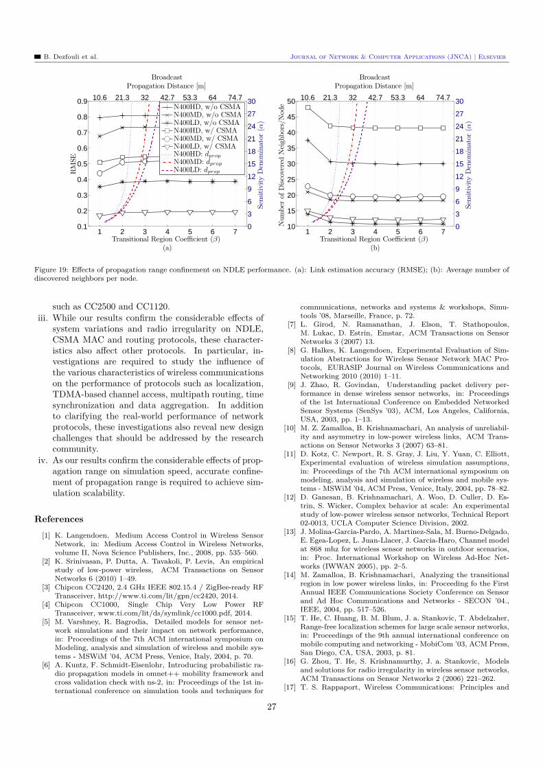
B. Dezfouli et al. Journal of Network & Computer Applications (JNCA) | Elsevier
1 2 3 4 5 6 70.1
0.2
0.3
0.4
0.5
0.6
0.7
0.8
0.9
RM
SE
Transitional Region Coefficient (β)(a)
BroadcastPropagation Distance [m]
10.6 21.3 32 42.7 53.3 64 74.7
0
3
6
9
12
15
18
21
24
27
30
Sen
sitivity
Den
omin
ator
(α)
N400HD, w/o CSMAN400MD, w/o CSMAN400LD, w/o CSMAN400HD, w/ CSMAN400MD, w/ CSMAN400LD, w/ CSMAN400HD: dprop
N400MD: dprop
N400LD: dprop
1 2 3 4 5 6 710
15
20
25
30
35
40
45
50
Num
ber
ofD
isco
vere
dN
eigh
bor
s/N
ode
Transitional Region Coefficient (β)(b)
BroadcastPropagation Distance [m]
10.6 21.3 32 42.7 53.3 64 74.7
0
3
6
9
12
15
18
21
24
27
30
Sen
sitivity
Den
omin
ator
(α)
Figure 19: Effects of propagation range confinement on NDLE performance. (a): Link estimation accuracy (RMSE); (b): Average number ofdiscovered neighbors per node.
such as CC2500 and CC1120.iii. While our results confirm the considerable effects of
system variations and radio irregularity on NDLE,CSMA MAC and routing protocols, these character-istics also affect other protocols. In particular, in-vestigations are required to study the influence ofthe various characteristics of wireless communicationson the performance of protocols such as localization,TDMA-based channel access, multipath routing, timesynchronization and data aggregation. In additionto clarifying the real-world performance of networkprotocols, these investigations also reveal new designchallenges that should be addressed by the researchcommunity.
iv. As our results confirm the considerable effects of prop-agation range on simulation speed, accurate confine-ment of propagation range is required to achieve sim-ulation scalability.
References
[1] K. Langendoen, Medium Access Control in Wireless SensorNetwork, in: Medium Access Control in Wireless Networks,volume II, Nova Science Publishers, Inc., 2008, pp. 535–560.
[2] K. Srinivasan, P. Dutta, A. Tavakoli, P. Levis, An empiricalstudy of low-power wireless, ACM Transactions on SensorNetworks 6 (2010) 1–49.
[3] Chipcon CC2420, 2.4 GHz IEEE 802.15.4 / ZigBee-ready RFTransceiver, http://www.ti.com/lit/gpn/cc2420, 2014.
[4] Chipcon CC1000, Single Chip Very Low Power RFTransceiver, www.ti.com/lit/ds/symlink/cc1000.pdf, 2014.
[5] M. Varshney, R. Bagrodia, Detailed models for sensor net-work simulations and their impact on network performance,in: Proceedings of the 7th ACM international symposium onModeling, analysis and simulation of wireless and mobile sys-tems - MSWiM ’04, ACM Press, Venice, Italy, 2004, p. 70.
[6] A. Kuntz, F. Schmidt-Eisenlohr, Introducing probabilistic ra-dio propagation models in omnet++ mobility framework andcross validation check with ns-2, in: Proceedings of the 1st in-ternational conference on simulation tools and techniques for
communications, networks and systems & workshops, Simu-tools ’08, Marseille, France, p. 72.
[7] L. Girod, N. Ramanathan, J. Elson, T. Stathopoulos,M. Lukac, D. Estrin, Emstar, ACM Transactions on SensorNetworks 3 (2007) 13.
[8] G. Halkes, K. Langendoen, Experimental Evaluation of Sim-ulation Abstractions for Wireless Sensor Network MAC Pro-tocols, EURASIP Journal on Wireless Communications andNetworking 2010 (2010) 1–11.
[9] J. Zhao, R. Govindan, Understanding packet delivery per-formance in dense wireless sensor networks, in: Proceedingsof the 1st International Conference on Embedded NetworkedSensor Systems (SenSys ’03), ACM, Los Angeles, California,USA, 2003, pp. 1–13.
[10] M. Z. Zamalloa, B. Krishnamachari, An analysis of unreliabil-ity and asymmetry in low-power wireless links, ACM Trans-actions on Sensor Networks 3 (2007) 63–81.
[11] D. Kotz, C. Newport, R. S. Gray, J. Liu, Y. Yuan, C. Elliott,Experimental evaluation of wireless simulation assumptions,in: Proceedings of the 7th ACM international symposium onmodeling, analysis and simulation of wireless and mobile sys-tems - MSWiM ’04, ACM Press, Venice, Italy, 2004, pp. 78–82.
[12] D. Ganesan, B. Krishnamachari, A. Woo, D. Culler, D. Es-trin, S. Wicker, Complex behavior at scale: An experimentalstudy of low-power wireless sensor networks, Technical Report02-0013, UCLA Computer Science Division, 2002.
[13] J. Molina-Garcia-Pardo, A. Martinez-Sala, M. Bueno-Delgado,E. Egea-Lopez, L. Juan-Llacer, J. Garcia-Haro, Channel modelat 868 mhz for wireless sensor networks in outdoor scenarios,in: Proc. International Workshop on Wireless Ad-Hoc Net-works (IWWAN 2005), pp. 2–5.
[14] M. Zamalloa, B. Krishnamachari, Analyzing the transitionalregion in low power wireless links, in: Proceeding fo the FirstAnnual IEEE Communications Society Conference on Sensorand Ad Hoc Communications and Networks - SECON ’04.,IEEE, 2004, pp. 517–526.
[15] T. He, C. Huang, B. M. Blum, J. a. Stankovic, T. Abdelzaher,Range-free localization schemes for large scale sensor networks,in: Proceedings of the 9th annual international conference onmobile computing and networking - MobiCom ’03, ACM Press,San Diego, CA, USA, 2003, p. 81.
[16] G. Zhou, T. He, S. Krishnamurthy, J. a. Stankovic, Modelsand solutions for radio irregularity in wireless sensor networks,ACM Transactions on Sensor Networks 2 (2006) 221–262.
[17] T. S. Rappaport, Wireless Communications: Principles and
27
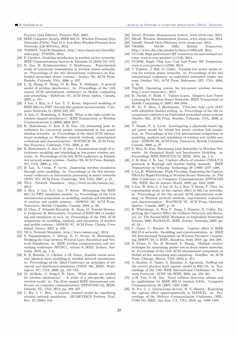
B. Dezfouli et al. Journal of Network & Computer Applications (JNCA) | Elsevier
Practice (2nd Edition), Prentice Hall, 2002.[18] IEEE Computer Society, IEEE 802.15: Wireless Personal Area
Networks (PANs). Part 15.4: Low-Rate Wireless Personal AreaNetworks (LR-WPANs), 2012.
[19] TOSSIM, TinyOS Simulator, http://docs.tinyos.net/tinywiki/index.php/ TOSSIM, 2014.
[20] P. Cardieri, Modeling interference in wireless ad hoc networks,IEEE Communications Surveys & Tutorials 12 (2010) 551–572.
[21] D. Son, B. Krishnamachari, J. Heidemann, Experimentalstudy of concurrent transmission in wireless sensor networks,in: Proceedings of the 4th international conference on Em-bedded networked sensor systems - SenSys ’06, ACM Press,Boulder, Colorado, USA, 2006, p. 237.
[22] L. Q. Zhang, F. Wang, M. K. Han, R. Mahajan, A generalmodel of wireless interference, in: Proceedings of the 13thannual ACM international conference on Mobile computingand networking - MobiCom ’07, ACM Press, Qubec, Canada,2007, p. 171.
[23] J. Lee, J. Ryu, S.-J. Lee, T. T. Kwon, Improved modeling ofIEEE 802.11a PHY through fine-grained measurements, Com-puter Networks 54 (2010) 641–657.
[24] A. Iyer, C. Rosenberg, A. Karnik, What is the right model forwireless channel interference?, IEEE Transactions on WirelessCommunications 8 (2009) 2662–2671.
[25] R. Maheshwari, S. Jain, S. R. Das, On estimating joint in-terference for concurrent packet transmissions in low powerwireless networks, in: Proceedings of the third ACM interna-tional workshop on Wireless network testbeds, experimentalevaluation and characterization - WiNTECH ’08, ACM Press,San Francisco, California, USA, 2008, p. 89.
[26] R. Maheshwari, S. Jain, S. R. Das, A measurement study of in-terference modeling and scheduling in low-power wireless net-works, in: Proceedings of the 6th ACM conference on Embed-ded network sensor systems - SenSys ’08, ACM Press, Raleigh,NC, USA, 2008, p. 141.
[27] H. Lee, A. Cerpa, P. Levis, Improving wireless simulationthrough noise modeling, in: Proceedings of the 6th interna-tional conference on Information processing in sensor networks(IPSN ’07), ACM Press, Cambridge, MA, USA, 2007, p. 21.
[28] NS-2, Network Simulator, http://www.isi.edu/nsnam/ns/,2014.
[29] J. Ryu, J. Lee, S.-J. Lee, T. Kwon, Revamping the IEEE802.11a PHY simulation models, in: Proceedings of the 11thinternational symposium on modeling, analysis and simulationof wireless and mobile systems - MSWIM ’08, ACM Press,Vancouver, British Columbia, Canada, 2008, p. 28.
[30] Q. Chen, F. Schmidt-Eisenlohr, D. Jiang, M. Torrent-Moreno,L. Delgrossi, H. Hartenstein, Overhaul of IEEE 802.11 model-ing and simulation in ns-2, in: Proceedings of the 10th ACMsymposium on modeling, analysis, and simulation of wirelessand mobile systems - MSWiM ’07, ACM Press, Chania, CreteIsland, Greece, 2007, p. 159.
[31] NS-3, Network Simulator, http://www.nsnam.org/, 2014.[32] S. Papanastasiou, J. Mittag, E. G. Strom, H. Hartenstein,
Bridging the Gap between Physical Layer Emulation and Net-work Simulation, in: IEEE wireless communication and net-working conference (WCNC), volume 9, IEEE, Sydney, Aus-tralia, 2010, pp. 1–6.
[33] E. B. Hamida, G. Chelius, J.-M. Gorce, Scalable versus accu-rate physical layer modeling in wireless network simulations,in: Proceedings of the 22nd Conference on principles of ad-vanced and distributed simulation (PADS ’08), IEEE, Wash-ington, DC, USA, 2008, pp. 127–134.
[34] M. Al-Bado, C. Sengul, R. Merz, What details are neededfor wireless simulations? - A study of a site-specific indoorwireless model, in: The 31rst annual IEEE international con-ference on computer communications (INFOCOM’12), IEEE,Orlando, FL, USA, 2012, pp. 289–297.
[35] C. Hu, J. C. Hou, A reactive channel model for expeditingwireless network simulation, SIGMETRICS Perform. Eval.Rev. 33 (2005) 410.
[36] Mica2, Wireless Measurement System, www.xbow.com, 2014.[37] MicaZ, Wireless Measurement System, www.xbow.com, 2014.[38] TelosB, TelosB Mote Platform, www.xbow.com, 2014.[39] TR1000, 916.50 MHz Hybrid Transceiver,
http://www.rfm.com/products/data/tr1000.pdf, 2014.[40] CC1120, High performance RF transceiver for narrowband sys-
tems, www.ti.com/product/cc1120, 2014.[41] CC2500, Single Chip Low Cost Low Power RF Transceiver,
www.ti.com/product/cc2500, 2014.[42] J. Polastre, J. Hill, D. Culler, Versatile low power media ac-
cess for wireless sensor networks, in: Proceedings of the 2ndinternational conference on embedded networked sensor sys-tems (SenSys ’04), ACM Press, Baltimore, MD, USA, 2004,p. 95.
[43] TinyOS, Operating system for low-power wireless devices,http://www.tinyos.net/, 2013.
[44] R. Jurdak, P. Baldi, C. Videira Lopes, Adaptive Low PowerListening for Wireless Sensor Networks, IEEE Transactions onMobile Computing 6 (2007) 988–1004.
[45] W. Ye, F. Silva, J. Heidemann, Ultra-low duty cycle MACwith scheduled channel polling, in: Proceedings of the 4th in-ternational conference on Embedded networked sensor systems(SenSys ’06), ACM Press, Boulder, Colorado, USA, 2006, p.321.
[46] T. Rusak, P. A. Levis, Investigating a physically-based sig-nal power model for robust low power wireless link simula-tion, in: Proceedings of the 11th international symposium onmodeling, analysis and simulation of wireless and mobile sys-tems - MSWiM ’08, ACM Press, Vancouver, British Columbia,Canada, 2008, p. 37.
[47] S. Woo, H. Kim, Estimating Link Reliability in Wireless Net-works: An Empirical Study and Interference Modeling, in:Proceedings IEEE INFOCOM’10, IEEE, 2010, pp. 1–5.
[48] J. H. Kim, J. K. Lee, Capture effects of wireless CSMA/CAprotocols in Rayleigh and shadow fading channels, IEEETransactions on Vehicular Technology 48 (1999) 1277–1286.
[49] J. Lu, K. Whitehouse, Flash Flooding: Exploiting the CaptureEffect for Rapid Flooding in Wireless Sensor Networks, in: The28th Conference on Computer Communications (INFOCOM’09), IEEE, Rio de Janeiro, Brazil, 2009, pp. 2491–2499.
[50] J. Lee, W. Kim, S.-J. Lee, D. Jo, J. Ryu, T. Kwon, Y. Choi, Anexperimental study on the capture effect in 802.11a networks,in: Proceedings of the the second ACM international work-shop on Wireless network testbeds, experimental evaluationand characterization - WinTECH ’07, ACM Press, Montreal,Quebec, Canada, 2007, p. 19.
[51] K. Whitehouse, A. Woo, F. Jiang, J. Polastre, D. Culler, Ex-ploiting the Capture Effect for Collision Detection and Recov-ery, in: The Second IEEE Workshop on Embedded NetworkedSensors, 2005. EmNetS-II., IEEE, Sydney, Australia, 2005, pp.45–52.
[52] C. Gezer, C. Buratti, R. Verdone, Capture effect in IEEE802.15.4 networks: Modelling and experimentation, in: IEEE5th International Symposium on Wireless Pervasive Comput-ing, ISWPC’10, ii, IEEE, Mondena, Italy, 2010, pp. 204–209.
[53] B. Firner, C. Xu, R. Howard, Y. Zhang, Multiple receiverstrategies for minimizing packet loss in dense sensor networks,in: Proceedings of the 11th ACM international symposium onMobile ad hoc networking and computing - MobiHoc ’10, ACMPress, Chicago, Illinois, USA, 2010, p. 211.
[54] A. Kochut, A. Vasan, A. Shankar, A. Agrawala, Sniffing outthe correct physical layer capture model in 802.11b, in: Pro-ceedings of the 12th IEEE International Conference on Net-work Protocols - ICNP ’04, IEEE, 2004, pp. 252–261.
[55] J.-H. Yun, S.-W. Seo, Novel collision detection scheme andits applications for IEEE 802.11 wireless LANs, ComputerCommunications 30 (2007) 1350–1366.
[56] H. Xu, J. J. Garcia-Luna-Aceves, R. S. Hamid, Exploitingthe capture effect opportunistically in MANETs, in: Pro-ceedings of the Military Communication Conference (MIL-COM’10), IEEE, San Jose, CA, USA, 2010, pp. 1490–1495.
28
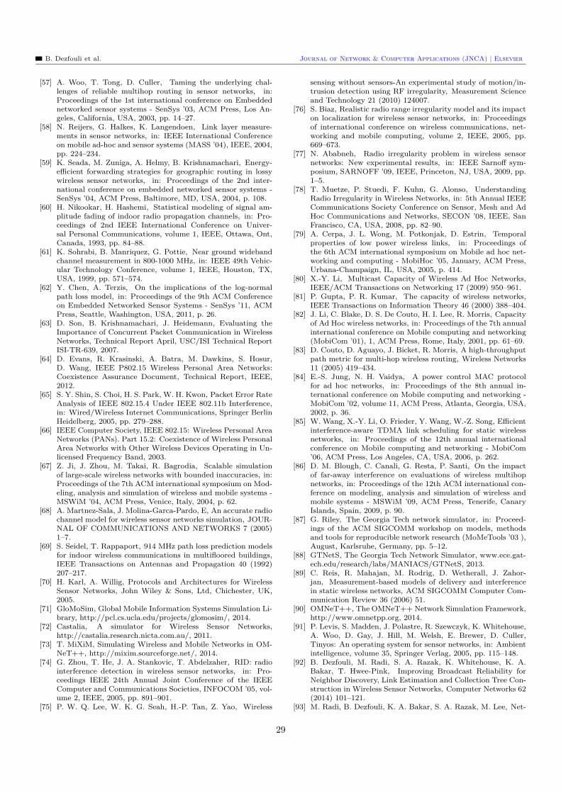
B. Dezfouli et al. Journal of Network & Computer Applications (JNCA) | Elsevier
[57] A. Woo, T. Tong, D. Culler, Taming the underlying chal-lenges of reliable multihop routing in sensor networks, in:Proceedings of the 1st international conference on Embeddednetworked sensor systems - SenSys ’03, ACM Press, Los An-geles, California, USA, 2003, pp. 14–27.
[58] N. Reijers, G. Halkes, K. Langendoen, Link layer measure-ments in sensor networks, in: IEEE International Conferenceon mobile ad-hoc and sensor systems (MASS ’04), IEEE, 2004,pp. 224–234.
[59] K. Seada, M. Zuniga, A. Helmy, B. Krishnamachari, Energy-efficient forwarding strategies for geographic routing in lossywireless sensor networks, in: Proceedings of the 2nd inter-national conference on embedded networked sensor systems -SenSys ’04, ACM Press, Baltimore, MD, USA, 2004, p. 108.
[60] H. Nikookar, H. Hashemi, Statistical modeling of signal am-plitude fading of indoor radio propagation channels, in: Pro-ceedings of 2nd IEEE International Conference on Univer-sal Personal Communications, volume 1, IEEE, Ottawa, Ont,Canada, 1993, pp. 84–88.
[61] K. Sohrabi, B. Manriquez, G. Pottie, Near ground widebandchannel measurement in 800-1000 MHz, in: IEEE 49th Vehic-ular Technology Conference, volume 1, IEEE, Houston, TX,USA, 1999, pp. 571–574.
[62] Y. Chen, A. Terzis, On the implications of the log-normalpath loss model, in: Proceedings of the 9th ACM Conferenceon Embedded Networked Sensor Systems - SenSys ’11, ACMPress, Seattle, Washington, USA, 2011, p. 26.
[63] D. Son, B. Krishnamachari, J. Heidemann, Evaluating theImportance of Concurrent Packet Communication in WirelessNetworks, Technical Report April, USC/ISI Technical ReportISI-TR-639, 2007.
[64] D. Evans, R. Krasinski, A. Batra, M. Dawkins, S. Hosur,D. Wang, IEEE P802.15 Wireless Personal Area Networks:Coexistence Assurance Document, Technical Report, IEEE,2012.
[65] S. Y. Shin, S. Choi, H. S. Park, W. H. Kwon, Packet Error RateAnalysis of IEEE 802.15.4 Under IEEE 802.11b Interference,in: Wired/Wireless Internet Communications, Springer BerlinHeidelberg, 2005, pp. 279–288.
[66] IEEE Computer Society, IEEE 802.15: Wireless Personal AreaNetworks (PANs). Part 15.2: Coexistence of Wireless PersonalArea Networks with Other Wireless Devices Operating in Un-licensed Frequency Band, 2003.
[67] Z. Ji, J. Zhou, M. Takai, R. Bagrodia, Scalable simulationof large-scale wireless networks with bounded inaccuracies, in:Proceedings of the 7th ACM international symposium on Mod-eling, analysis and simulation of wireless and mobile systems -MSWiM ’04, ACM Press, Venice, Italy, 2004, p. 62.
[68] A. Martnez-Sala, J. Molina-Garca-Pardo, E, An accurate radiochannel model for wireless sensor networks simulation, JOUR-NAL OF COMMUNICATIONS AND NETWORKS 7 (2005)1–7.
[69] S. Seidel, T. Rappaport, 914 MHz path loss prediction modelsfor indoor wireless communications in multifloored buildings,IEEE Transactions on Antennas and Propagation 40 (1992)207–217.
[70] H. Karl, A. Willig, Protocols and Architectures for WirelessSensor Networks, John Wiley & Sons, Ltd, Chichester, UK,2005.
[71] GloMoSim, Global Mobile Information Systems Simulation Li-brary, http://pcl.cs.ucla.edu/projects/glomosim/, 2014.
[72] Castalia, A simulator for Wireless Sensor Networks,http://castalia.research.nicta.com.au/, 2011.
[73] T. MiXiM, Simulating Wireless and Mobile Networks in OM-NeT++, http://mixim.sourceforge.net/, 2014.
[74] G. Zhou, T. He, J. A. Stankovic, T. Abdelzaher, RID: radiointerference detection in wireless sensor networks, in: Pro-ceedings IEEE 24th Annual Joint Conference of the IEEEComputer and Communications Societies, INFOCOM ’05, vol-ume 2, IEEE, 2005, pp. 891–901.
[75] P. W. Q. Lee, W. K. G. Seah, H.-P. Tan, Z. Yao, Wireless
sensing without sensors-An experimental study of motion/in-trusion detection using RF irregularity, Measurement Scienceand Technology 21 (2010) 124007.
[76] S. Biaz, Realistic radio range irregularity model and its impacton localization for wireless sensor networks, in: Proceedingsof international conference on wireless communications, net-working and mobile computing, volume 2, IEEE, 2005, pp.669–673.
[77] N. Ababneh, Radio irregularity problem in wireless sensornetworks: New experimental results, in: IEEE Sarnoff sym-posium, SARNOFF ’09, IEEE, Princeton, NJ, USA, 2009, pp.1–5.
[78] T. Muetze, P. Stuedi, F. Kuhn, G. Alonso, UnderstandingRadio Irregularity in Wireless Networks, in: 5th Annual IEEECommunications Society Conference on Sensor, Mesh and AdHoc Communications and Networks, SECON ’08, IEEE, SanFrancisco, CA, USA, 2008, pp. 82–90.
[79] A. Cerpa, J. L. Wong, M. Potkonjak, D. Estrin, Temporalproperties of low power wireless links, in: Proceedings ofthe 6th ACM international symposium on Mobile ad hoc net-working and computing - MobiHoc ’05, January, ACM Press,Urbana-Champaign, IL, USA, 2005, p. 414.
[80] X.-Y. Li, Multicast Capacity of Wireless Ad Hoc Networks,IEEE/ACM Transactions on Networking 17 (2009) 950–961.
[81] P. Gupta, P. R. Kumar, The capacity of wireless networks,IEEE Transactions on Information Theory 46 (2000) 388–404.
[82] J. Li, C. Blake, D. S. De Couto, H. I. Lee, R. Morris, Capacityof Ad Hoc wireless networks, in: Proceedings of the 7th annualinternational conference on Mobile computing and networking(MobiCom ’01), 1, ACM Press, Rome, Italy, 2001, pp. 61–69.
[83] D. Couto, D. Aguayo, J. Bicket, R. Morris, A high-throughputpath metric for multi-hop wireless routing, Wireless Networks11 (2005) 419–434.
[84] E.-S. Jung, N. H. Vaidya, A power control MAC protocolfor ad hoc networks, in: Proceedings of the 8th annual in-ternational conference on Mobile computing and networking -MobiCom ’02, volume 11, ACM Press, Atlanta, Georgia, USA,2002, p. 36.
[85] W. Wang, X.-Y. Li, O. Frieder, Y. Wang, W.-Z. Song, Efficientinterference-aware TDMA link scheduling for static wirelessnetworks, in: Proceedings of the 12th annual internationalconference on Mobile computing and networking - MobiCom’06, ACM Press, Los Angeles, CA, USA, 2006, p. 262.
[86] D. M. Blough, C. Canali, G. Resta, P. Santi, On the impactof far-away interference on evaluations of wireless multihopnetworks, in: Proceedings of the 12th ACM international con-ference on modeling, analysis and simulation of wireless andmobile systems - MSWiM ’09, ACM Press, Tenerife, CanaryIslands, Spain, 2009, p. 90.
[87] G. Riley, The Georgia Tech network simulator, in: Proceed-ings of the ACM SIGCOMM workshop on models, methodsand tools for reproducible network research (MoMeTools ’03 ),August, Karlsruhe, Germany, pp. 5–12.
[88] GTNetS, The Georgia Tech Network Simulator, www.ece.gat-ech.edu/research/labs/MANIACS/GTNetS, 2013.
[89] C. Reis, R. Mahajan, M. Rodrig, D. Wetherall, J. Zahor-jan, Measurement-based models of delivery and interferencein static wireless networks, ACM SIGCOMM Computer Com-munication Review 36 (2006) 51.
[90] OMNeT++, The OMNeT++ Network Simulation Framework,http://www.omnetpp.org, 2014.
[91] P. Levis, S. Madden, J. Polastre, R. Szewczyk, K. Whitehouse,A. Woo, D. Gay, J. Hill, M. Welsh, E. Brewer, D. Culler,Tinyos: An operating system for sensor networks, in: Ambientintelligence, volume 35, Springer Verlag, 2005, pp. 115–148.
[92] B. Dezfouli, M. Radi, S. A. Razak, K. Whitehouse, K. A.Bakar, T. Hwee-Pink, Improving Broadcast Reliability forNeighbor Discovery, Link Estimation and Collection Tree Con-struction in Wireless Sensor Networks, Computer Networks 62(2014) 101–121.
[93] M. Radi, B. Dezfouli, K. A. Bakar, S. A. Razak, M. Lee, Net-
29
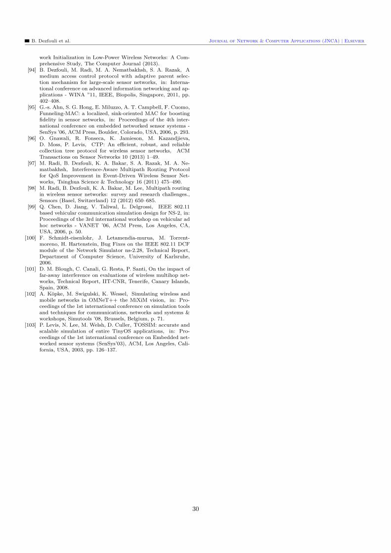
B. Dezfouli et al. Journal of Network & Computer Applications (JNCA) | Elsevier
work Initialization in Low-Power Wireless Networks: A Com-prehensive Study, The Computer Journal (2013).
[94] B. Dezfouli, M. Radi, M. A. Nematbakhsh, S. A. Razak, Amedium access control protocol with adaptive parent selec-tion mechanism for large-scale sensor networks, in: Interna-tional conference on advanced information networking and ap-plications - WINA ”11, IEEE, Biopolis, Singapore, 2011, pp.402–408.
[95] G.-s. Ahn, S. G. Hong, E. Miluzzo, A. T. Campbell, F. Cuomo,Funneling-MAC: a localized, sink-oriented MAC for boostingfidelity in sensor networks, in: Proceedings of the 4th inter-national conference on embedded networked sensor systems -SenSys ’06, ACM Press, Boulder, Colorado, USA, 2006, p. 293.
[96] O. Gnawali, R. Fonseca, K. Jamieson, M. Kazandjieva,D. Moss, P. Levis, CTP: An efficient, robust, and reliablecollection tree protocol for wireless sensor networks, ACMTransactions on Sensor Networks 10 (2013) 1–49.
[97] M. Radi, B. Dezfouli, K. A. Bakar, S. A. Razak, M. A. Ne-matbakhsh, Interference-Aware Multipath Routing Protocolfor QoS Improvement in Event-Driven Wireless Sensor Net-works, Tsinghua Science & Technology 16 (2011) 475–490.
[98] M. Radi, B. Dezfouli, K. A. Bakar, M. Lee, Multipath routingin wireless sensor networks: survey and research challenges.,Sensors (Basel, Switzerland) 12 (2012) 650–685.
[99] Q. Chen, D. Jiang, V. Taliwal, L. Delgrossi, IEEE 802.11based vehicular communication simulation design for NS-2, in:Proceedings of the 3rd international workshop on vehicular adhoc networks - VANET ’06, ACM Press, Los Angeles, CA,USA, 2006, p. 50.
[100] F. Schmidt-eisenlohr, J. Letamendia-murua, M. Torrent-moreno, H. Hartenstein, Bug Fixes on the IEEE 802.11 DCFmodule of the Network Simulator ns-2.28, Technical Report,Department of Computer Science, University of Karlsruhe,2006.
[101] D. M. Blough, C. Canali, G. Resta, P. Santi, On the impact offar-away interference on evaluations of wireless multihop net-works, Technical Report, IIT-CNR, Tenerife, Canary Islands,Spain, 2008.
[102] A. Köpke, M. Swigulski, K. Wessel, Simulating wireless andmobile networks in OMNeT++ the MiXiM vision, in: Pro-ceedings of the 1st international conference on simulation toolsand techniques for communications, networks and systems &workshops, Simutools ’08, Brussels, Belgium, p. 71.
[103] P. Levis, N. Lee, M. Welsh, D. Culler, TOSSIM: accurate andscalable simulation of entire TinyOS applications, in: Pro-ceedings of the 1st international conference on Embedded net-worked sensor systems (SenSys’03), ACM, Los Angeles, Cali-fornia, USA, 2003, pp. 126–137.
30