University of Tennessee, Knoxville University of Tennessee, Knoxville

TRACE: Tennessee Research and Creative TRACE: Tennessee Research and Creative

Exchange Exchange

Masters Theses Graduate School

5-2003

A Study of the Electron Beam Scattering Under Various Gaseous A Study of the Electron Beam Scattering Under Various Gaseous

Environment Environment

Jing He University of Tennessee - Knoxville

Follow this and additional works at: https://trace.tennessee.edu/utk_gradthes

Part of the Engineering Science and Materials Commons

Recommended Citation Recommended Citation He, Jing, "A Study of the Electron Beam Scattering Under Various Gaseous Environment. " Master's Thesis, University of Tennessee, 2003. https://trace.tennessee.edu/utk_gradthes/1971

This Thesis is brought to you for free and open access by the Graduate School at TRACE: Tennessee Research and Creative Exchange. It has been accepted for inclusion in Masters Theses by an authorized administrator of TRACE: Tennessee Research and Creative Exchange. For more information, please contact trace@utk.edu.

To the Graduate Council:

I am submitting herewith a thesis written by Jing He entitled "A Study of the Electron Beam

Scattering Under Various Gaseous Environment." I have examined the final electronic copy of

this thesis for form and content and recommend that it be accepted in partial fulfillment of the

requirements for the degree of Master of Science, with a major in Materials Science and

Engineering.

David C. Joy, Major Professor

We have read this thesis and recommend its acceptance:

R.A.Buchanan, Robert Mee

Accepted for the Council:

Carolyn R. Hodges

Vice Provost and Dean of the Graduate School

(Original signatures are on file with official student records.)

To the Graduate Council:

I am submitting here with a thesis written by Jing He entitled " A study of the electron

beam scattering under various gaseous environment." I have examined the final

electronic copy of this thesis for form and content and recommend that it be accepted in

partial fulfillment of the requirements for the degree of Master of Science, with a major

in Material Science and Engineering.

David C. Joy

——————————

Major Professor

We have read this thesis

and recommend its acceptance:

R.A.Buchanan, ————————— Professor Robert Mee, ————————— Professor

Accepted for the Council:

Anne Mayhew

——————————————

Vice Provost and Dean of Graduate

Studies

(Original signatures are on file with official student records.)

A STUDY

OF THE ELECTRON BEAM SCATTERING

UNDER VARIOUS GASEOUS ENVIRONMENT

A Thesis Presented for the

Master of Science Degree

The University of Tennessee, Knoxville

Jing He

May 2003

DEDICATION

This thesis is dedicated to my loving husband, Hongbo Tian,

who has always been giving me strength and courage to achieve my goals; and

love and happiness to live a wonderful life.

I also dedicate this wok to my parents, Yao He and Yuhua Fan,

great role models, and without whose devotion and inspiration I will never be the

person I am today.

ii

ACKNOWLEDGMENTS

Words can never express my deepest gratitude to my academic advisor Dr.

D. C. Joy. Not only is he a distinguished scientist full of brilliant ideas, but also a

wonderful instructor whose great enthusiasm, guidance, inspiration and support

help me see and learn extraordinary things. I would also like to express my

sincere appreciation to my committee members, Dr. R.A Buchanan and Dr.

Robert Mee, for being highly supportive and instructive on my master program.

I wish to thank everybody in our EM lab, for making my time as a

graduate student here exceptional memorable. Truly thanks to Xiaohu Tang and

Satya M. Prasad for their genuine friendship and always being there for me.

Thanks to Mr. Toshihide Agemura for his strong technical support on the

Scanning Electron Microscope and Mr. Douglas Fielden for mechanical parts

processing. I would also like to thank Dr. Carolyn and Dr. John Dunlap for their

grand helps in lab equipment and materials, and to Jennifer Trollinger for her

kindness and continuous assistance on everything. My thanks also go to Dr.

Yeong-Uk Ko, Young Choi and Alexander Thesen for their support.

I would also like to thank my family and all my friends for always

believing in me, encouraging me and supporting me to make today possible.

iii

ABSTRACT

There are three objectives in this work: to experimentally measure the profiles of

electron beams scattered by interaction with a gas, to measure total scattering cross-

sections for gases and to apply the cross-section data in a suitable Monte Carlo simulation

to predict beam scattering profiles for comparison with experiment.

The experimentally measured profiles cover a wide range of intensity variation.

There are two evidenced regions: an inner region and an outer skirt corresponding to

inelastic (small angle) and elastic scattering respectively are appeared. These profiles use

the planar p-n junction gives us an overall look at the electron beam spreading, including

the oversize and shape of the profile.

The experimental total scattering cross-section data obtained is of great interest.

It shows the excellent agreement between experimental values and theoretical estimates

of the total gas scattering cross-section and also confirms the predicted linear relationship

between log (Ip/I0) and gas pressure. On the basis of the available evidence, gases tend to

be molecular rather than atomic in nature in the pressure range used.

The experimentally collected gas scattering cross-section data eventually was

inserted into Monte Carlo simulation program. The established Monte Carlo simulation

predicts the spatial distribution of the electron beam scattering under given beam energy

and various other experimental conditions. The resulted beam profiles from the

simulation are well agreed with the experimental measured profiles, with much higher

accuracy and more variety of experimental conditions choices.

iv

TABLE OF CONTENTS

Chapter Page

I. INTRODUCTION 1

1.1 Electron Microscopy 1

1.2 Scanning Electron Microscopy 1

1.3 Gaseous Environmental Scanning Electron Microscope 4

1.3.1 Gaseous Environmental SEM 4

1.3.2 Charge Compensation by Gas 6

1.3.3 Direct Examination of Dirty and Wet Sample 9

1.3.4 Selectively Etching and Deposition by E-beam 9

1.4 Electron Beam Scattering 14

1.4.1 Scattering Introduction 14

1.4.2 Electron Beam Scattering by Gas 15

1.4.3 Gas scattering Cross-section Introduction 18

1.4.3.1 Definition of Cross-section 18

1.4.3.2 Rutherford and Mott Cross-section 22

1.4.3.3 Mean Free Path 23

II. DIRECTLY MEASUREMENT OF THE ELECTRON

BEAM SCATTERING 25

2.1 Introduction 25

2.2 Introduction of P-N Junction Solar Cell 25

2.3 Experimental Method 26

2.4 Experimental Procedure 29

2.5 Experimental Results and Discussion 32

2.6 Summary 32

III. MEASUREMENT OF TOTAL GAS SCATTERING

CROSS-SECTION 35

3.1 Introduction 35

3.2 Experimental Method 35

v

3.3 Experimental Procedure 37

3.4 Experimental Results 39

3.4.1 Linear Relationship of Ln (I) and P 39

3.4.2 Calculated Total Scattering Cross-sections 39

3.5 Discussion of Errors in the Procedure 49

3.5.1 Gas Pressure Measurement in the VPSEM 49

3.5.2 Confirmation of the Gas Path Length 51

3.5.3 Confirmation of the Temperature Variation 51

3.5.4 Possible Noise Signals from the Background 54

3.6 Experimental Results Discussion 56

3.7 Summary 59

IV. MONTE CARLO SIMULATION OF THE ELECTRON BEAM

SCATTERING 61

4.1 Introduction of Monte Carlo Simulation 61

4.1.1 Background Introduction 61

4.1.2 Random Number Sampling 63

4.2 Monte Carlo Simulation of Electrons Trajectories in a Solid 63

4.2.1 Basic Principle 64

4.2.2 Assumptions for Original Model 66

4.2.3 Statistics of the Original Model 66

4.3 New Monte Carlo Simulation for Gas 69

4.3.1 Why Use This Method 69

4.3.2 How We Did It 70

4.3.2.1 Include Inelastic and Elastic Scattering 70

4.3.2.2 Single Scattering Model 71

4.3.2.3 Energy Loss of the Incident Electrons 78

4.3.2.4 Schematic Sequence of the Operation 79

4.3.2.5 I(r) Radial Beam Distribution Plot 79

4.3.2.6 Computer Code 81

4.4 Simulation Results 81

4.5 Summary 86

vi

REFERENCES 89

APPENDIX 95

VITA 108

vii

LIST OF FIGURES

Figure Page

1.1 The comparison of SEM micrograph and optical micrograph

of the adiolarian Trochodiscus longispinus. 2

1.2 A standard ESEM column configuration. 5

1.3 Relationship between incident beam energy and surface charging. 7

1.4 Schematic of the ionizing collisions in a low-pressure gas

above a charged insulator. 8

1.5 IC examined in VPSEM under different air pressures. 10

1.6 Live cells and liquid specimen examined in ESEM. 11

1.7 E-beam deposition and etching for Silicon wafer. 12

1.8 Principle of EBD. 13

1.9 Schematic of scattering by a small particle. 14

1.10 Schematic of the scattering by surrounding gases in VPSEM. 17

1.11 The interaction cross-section for a particular process

compared with the geometric cross-section. 20

1.12 Schematic of the differential cross-section calculation. 21

1.13 Mean free path and kinetic energy. 24

2.1 Band structures of differently doped semiconductors. 27

2.2 Band-bending structure of hetero-junction. 27

2.3 Principle of photovoltaic device. 28

2.4 Schematic arrangement of measuring the beam profile in a SEM. 30

2.5 SE image of the positioned solar cell. 31

2.6 AE image detected by the solar cell. 31

2.7 Raw profile data collected at 15, 20, 25keV. 33

2.8 Scattered beam profiles in Air at E = 25keV after deconvolution. 34

3.1 Schematic of the experimental technique. 36

3.2 Experimental equipment (VPSEM, EDS, Manometer). 38

3.3 SEM image of the Al wire cross-section. 40

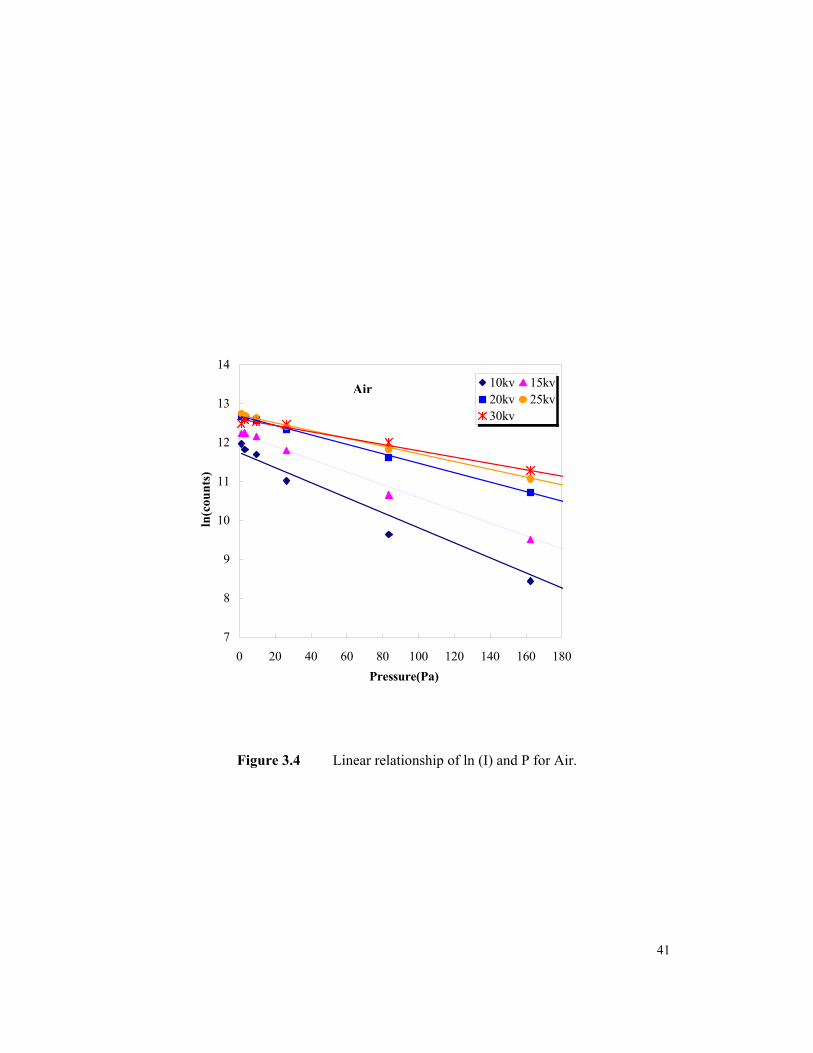
3.4 Linear relationship of ln (I) and P for Air. 41

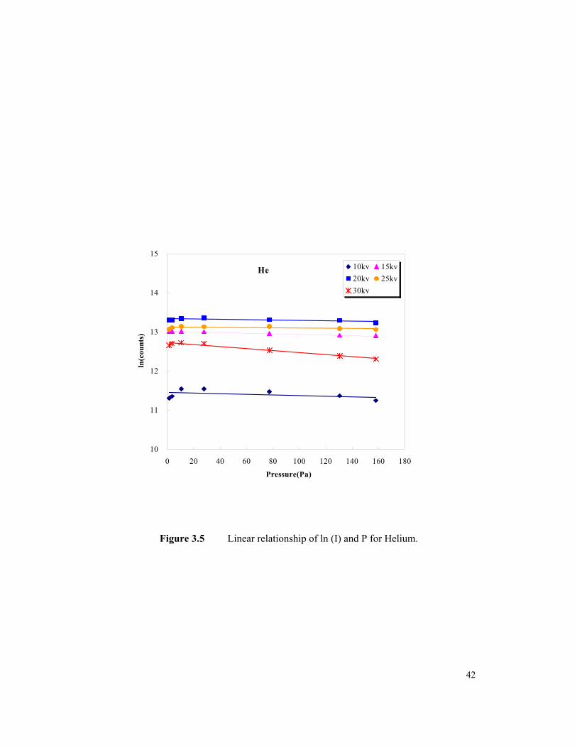
3.5 Linear relationship of ln (I) and P for Helium. 42

viii

ix

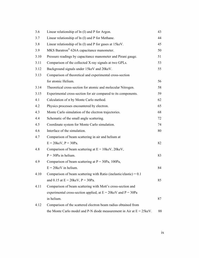
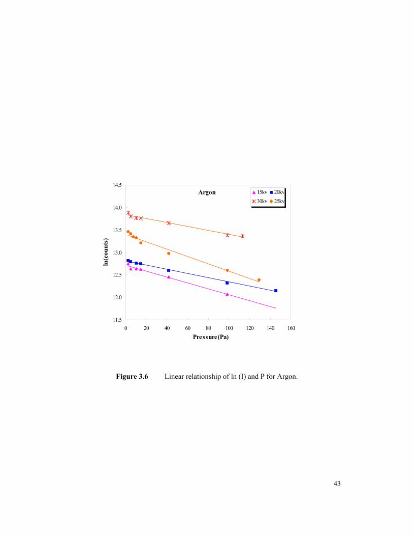
3.6 Linear relationship of ln (I) and P for Argon. 43

3.7 Linear relationship of ln (I) and P for Methane. 44

3.8 Linear relationship of ln (I) and P for gases at 15keV. 45

3.9 MKS Baratron® 626A capacitance manometer. 50

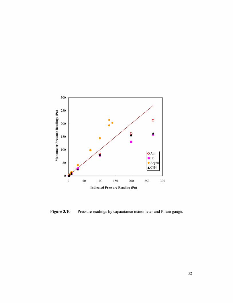
3.10 Pressure readings by capacitance manometer and Pirani gauge. 51

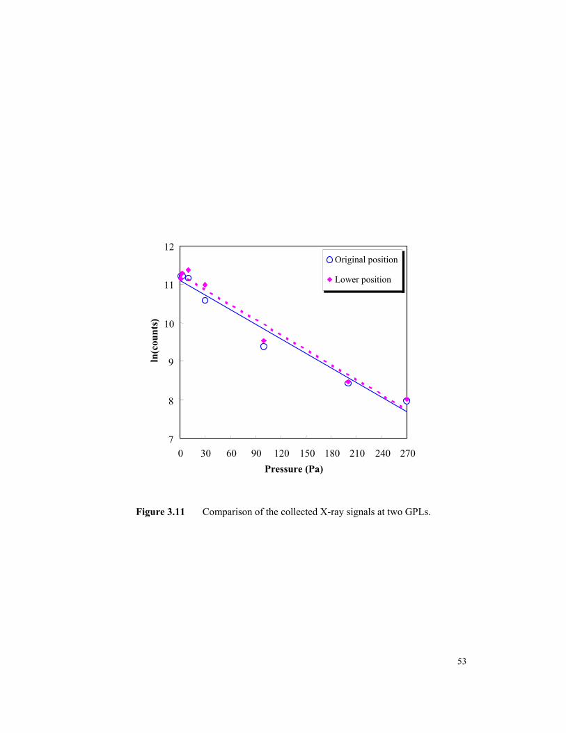
3.11 Comparison of the collected X-ray signals at two GPLs. 53

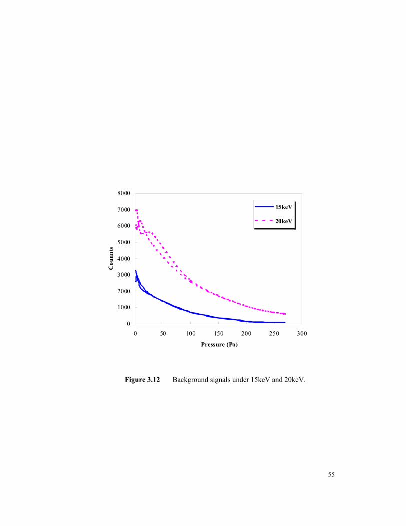
3.12 Background signals under 15keV and 20keV. 55

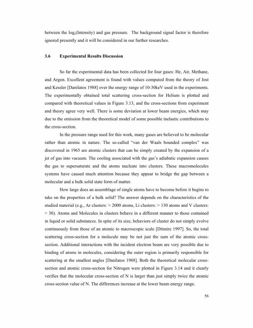
3.13 Comparison of theoretical and experimental cross-section

for atomic Helium. 56

3.14 Theoretical cross-section for atomic and molecular Nitrogen. 58

3.15 Experimental cross-section for air compared to its components. 59

4.1 Calculation of π by Monte Carlo method. 62

4.2 Physics processes encountered by electron. 65

4.3 Monte Carlo simulation of the electron trajectories. 68

4.4 Schematic of the small angle scattering. 72

4.5 Coordinate system for Monte Carlo simulation. 74

4.6 Interface of the simulation. 80

4.7 Comparison of beam scattering in air and helium at

E = 20keV, P = 30Pa. 82

4.8 Comparison of beam scattering at E = 10keV, 20keV,

P = 30Pa in helium. 83

4.9 Comparison of beam scattering at P = 30Pa, 100Pa,

E = 20keV in helium. 84

4.10 Comparison of beam scattering with Ratio (inelastic/elastic) = 0.1

and 0.15 at E = 20keV, P = 30Pa. 85

4.11 Comparison of beam scattering with Mott’s cross-section and

experimental cross-section applied, at E = 20keV and P = 30Pa

in helium. 87

4.12 Comparison of the scattered electron beam radius obtained from

the Monte Carlo model and P-N diode measurement in Air at E = 25keV. 88

CHAPTER I INTRODUCTION

1.1 Electron Microscopy

Electron microscopy is a very powerful technique which permits scientists to

observe, analyze and correctly explain phenomena occurring on a micrometer or

submicrometer scale. Electron microscope is analagous to light microscope where the

light beam is replaced by a beam of electrons. The electron beam is focussed by a series

of electrostatic or electromagnetic lenses. The types of signals produced when the

electron beam inpinges on a specimen sureface include secondary electrons,

backscattered electron, Auger electrons, characteristic x-rays, and photons of various

energies. These signals are obtained from specific emisssion volumes within the sample

and can be used to examine many characteristics of the interested samples, such as

compostition, surface topography and crystallography etc.

1.2 Scanning Electron Microscopy

The scanning electron microscopy (SEM) is one of the most versatile instruments

available for the examination and anlysis of the microstructural characteristics of solid

objects. In scanning electron microscopy the beam sweeps the surface of the sample

synchronised with a beam from a cathode ray tube. The signals of greatest interest here

are from secondary electrons and backscattered electrons. One of the major features of

the SEM is that the resolution can reach as high as 1 nm, and another is the three

dimensional appearance of the specimen image, due to the large depth of field as well as

to the shadow-relief effect of the secondary and backscattered electron contrast.

Compared with optical microscopy image, the image obtained in SEM has much greater

depth of focus and superior resolving capability as illustrated in Figure 1.1.

The magnification of SEM is determined by the size of the scanned surface area

in comparison to the size of the screen on which the image is projected, which is easy to

adjust because the variation of the magnification is only related with the change of the

geometry size of the image screen. Resolution depends on the size of the electron beam

1

25µm

(a)

(b)

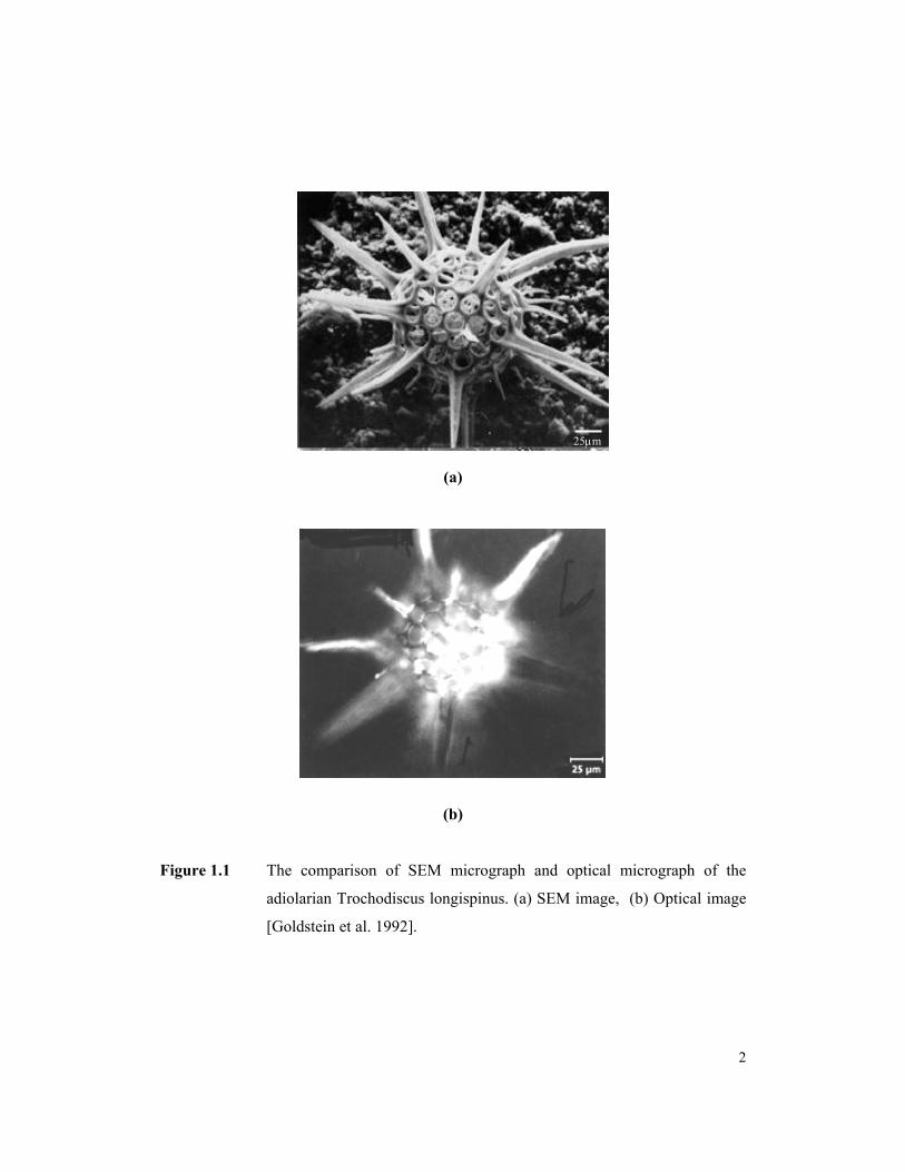
Figure 1.1 The comparison of SEM micrograph and optical micrograph of the

adiolarian Trochodiscus longispinus. (a) SEM image, (b) Optical image

[Goldstein et al. 1992].

2

and on the scattering volume within the sample but the depth of focus is because the

angle of convergence of the focussed beam is small.

One of the disadvantages for conventional scanning electron microscopes (SEM)

is that operation under high vacuum (<10-3Pa) is always strictly required, so sample to be

investigated must be clean, dry and free of volatile species and electrically conductive.

This has always been a limitation when the samples are materials with poor electrical

conductivity, such as semiconductor, IC chips, fibers, or some live cells with water vapor

components. Since these materials are playing a more and more important role in our

everyday lives and are widely used in various technology fields, such as pharmaceuticas,

fiber technology, cement science, medical, biology , entomology and microelectronics, a

new generation of SEM is urgently required.

Why are there such limitations? What happens when we put such specimen

inside the SEM chamber?

a. When an electron beam irradiates an insulator, a dielectric, or a semiconductor

during SEM observation, stored charges will build up on the specimen. The contrast of

the image thus may become abnormal and unstable, and the resolution of the image may

degrade. Charge accumulation in insulator or semiconductor materials due to electron

beam irradiation is one of the key problems in electron microscopy. Traditionally coating

a thin conductive layer on the sample surface is an effective way to eliminate charging,

but the coating may reduce topographic and chemical composition contrast, and obscure

crystallographic channeling patterns [Moncrieff et al 1978]. Reducing the incident beam

energy is another possible solution to charging since this can increase the SE yield from

the sample until the charge injected by the beam is balanced by the charge (SE+BSE)

emitted by the sample [Cazaux 1988]. However, lower beam energies may result in

poorer resolution, and there are practical problems in applying this method to an

inhomogeneous surface [Tang, 2002].

b. When a liquid and hydrated samples are directly examined inside the SEM

chamber, it will destroy the high vacuum environment required by conventional SEM and

also may contaminate the lenses and aperture in the system. Biological samples were

always, therefore, dehydrated before they are put into the SEM specimen chamber, which

results that the real characteristic of the sample can not be explored, and that live cells

could never be observed in conventional SEM.

3

With the fast growing interests of all these advanced materials in this new era of

science and technology, the electron microscopy technology is also developing rapidly to

adapt all the materials studies which are unsuitable for conventional SEM.

1.3 Gaseous Environmental Scanning Electron Microscope

A very promising family of Scanning Electron Microscopes (SEM) is those with

a low pressure of gas in the specimen chamber, such as the environmental scanning

electron microscope (ESEM) or the variable pressure scanning electron microscope

(VPSEM). These gaseous environment SEMs do not have the limitations on state of the

specimen. These machines offer the ability to image insulators and wet, dirty or damp

materials such as biological tissue, and even liquids without extra sample preparation and

coating.

1.3.1 Gaseous environmental SEM

Gaseous environmental SEM operates at relatively high pressures while the vast

majority of traditional microscopes operate at a vacuum below 10-2 pa. This includes a

variety of techniques reported in the scientific and commercial literature, e.g.,

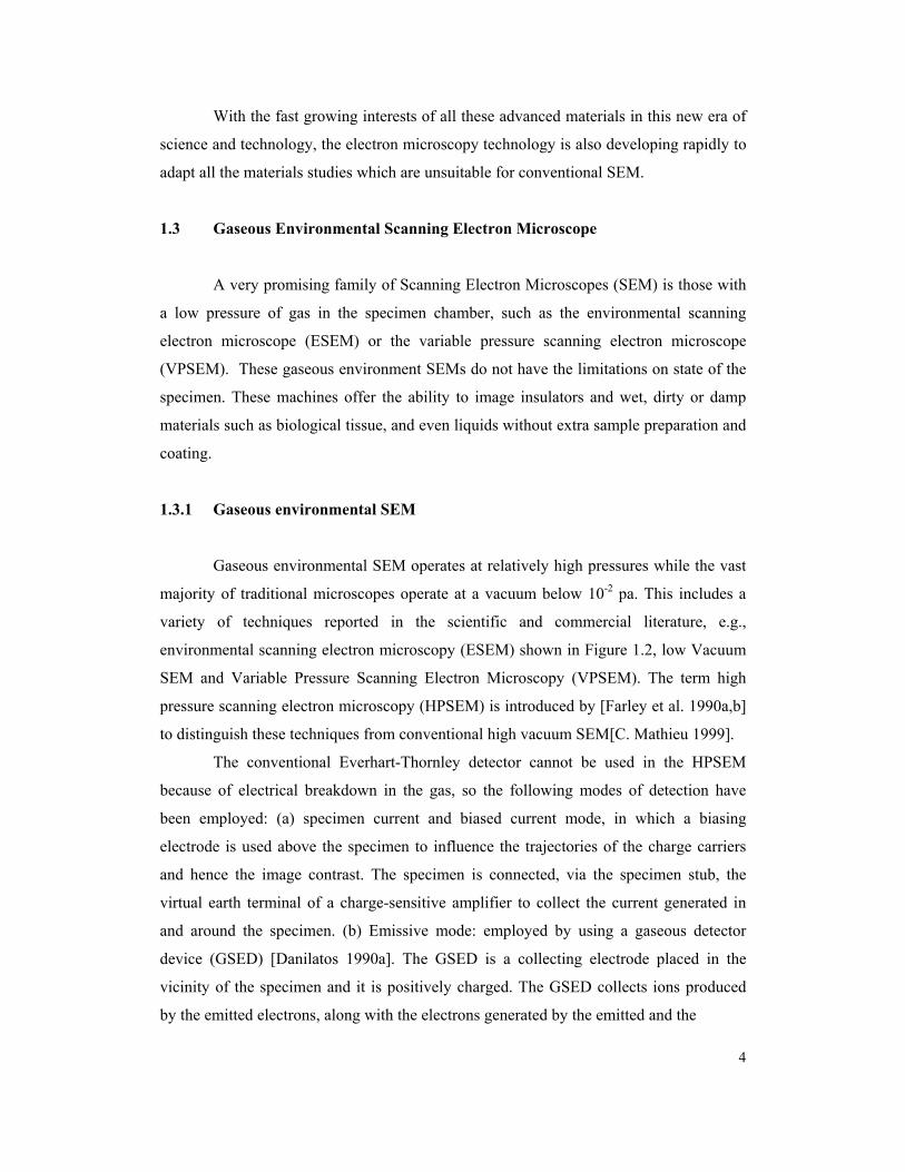
environmental scanning electron microscopy (ESEM) shown in Figure 1.2, low Vacuum

SEM and Variable Pressure Scanning Electron Microscopy (VPSEM). The term high

pressure scanning electron microscopy (HPSEM) is introduced by [Farley et al. 1990a,b]

to distinguish these techniques from conventional high vacuum SEM[C. Mathieu 1999].

The conventional Everhart-Thornley detector cannot be used in the HPSEM

because of electrical breakdown in the gas, so the following modes of detection have

been employed: (a) specimen current and biased current mode, in which a biasing

electrode is used above the specimen to influence the trajectories of the charge carriers

and hence the image contrast. The specimen is connected, via the specimen stub, the

virtual earth terminal of a charge-sensitive amplifier to collect the current generated in

and around the specimen. (b) Emissive mode: employed by using a gaseous detector

device (GSED) [Danilatos 1990a]. The GSED is a collecting electrode placed in the

vicinity of the specimen and it is positively charged. The GSED collects ions produced

by the emitted electrons, along with the electrons generated by the emitted and the

4

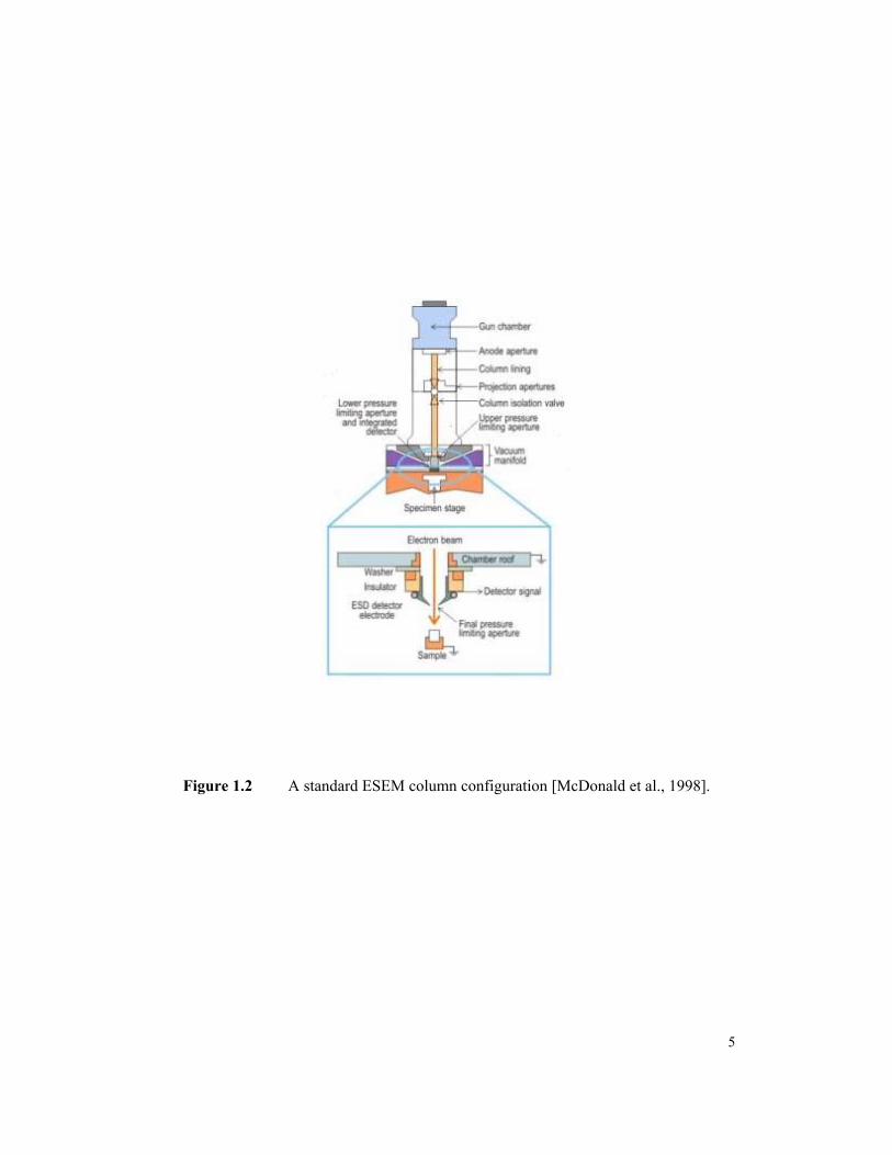
Figure 1.2 A standard ESEM column configuration [McDonald et al., 1998].

5

primary electrons. (c) Backscattered mode: Backscattered electron imaging with high gas

pressure in the specimen chamber has proven to be a useful technique and this technique

has been widely used in the Variable Pressure Scanning Electron Microscope (VPSEM)

[Mathieu 1996].

1.3.2 Charge Compensation by Gas

The gaseous environmental SEM allows observations to be carried out in the

presence of the low pressure gases. The gaseous environment inside the specimen

chamber during operation consists of low-energy secondary electrons, gas molecules, and

ions that have the added benefit of helping to drain the excess surface charge away

[Wight 2001], because the ionizations which occur in the gas as the result of electron

interactions produce a flux of positive ions which migrate to charged regions on the

surface and neutralize them. The suggested mechanism for the charge neutralization by

low pressure gases could be the continuous discharge by ionization currents resulting

from ion pairs formed by electron collisions with gas molecules [Moncrieff et al. 1978].

The need for conductive coatings is therefore reduced or eliminated when these poorly

conductive or insulator samples can be imaged at high beam energies (typically 10–30

keV) [Mohan et al. 1998].

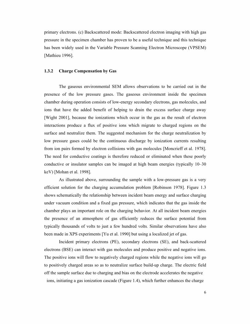
As illustrated above, surrounding the sample with a low-pressure gas is a very

efficient solution for the charging accumulation problem [Robinson 1978]. Figure 1.3

shows schematically the relationship between incident beam energy and surface charging

under vacuum condition and a fixed gas pressure, which indicates that the gas inside the

chamber plays an important role on the charging behavior. At all incident beam energies

the presence of an atmosphere of gas efficiently reduces the surface potential from

typically thousands of volts to just a few hundred volts. Similar observations have also

been made in XPS experiments [Yu et al. 1990] but using a localized jet of gas.

Incident primary electrons (PE), secondary electrons (SE), and back-scattered

electrons (BSE) can interact with gas molecules and produce positive and negative ions.

The positive ions will flow to negatively charged regions while the negative ions will go

to positively charged areas so as to neutralize surface build-up charge. The electric field

off the sample surface due to charging and bias on the electrode accelerates the negative

ions, initiating a gas ionization cascade (Figure 1.4), which further enhances the charge

6

10 15 20 25 300

-1

-2

-3

-4

-5

-6

-7

-8

Low Vacuum

High Vacuum

Surf

ace

char

ging

(keV

)

Beam energy (keV)

Figure 1.3 Relationship between incident beam energy and surface charging.

7

SE

Field

PE

BSE

Ion

ESE

Gas

Insulator

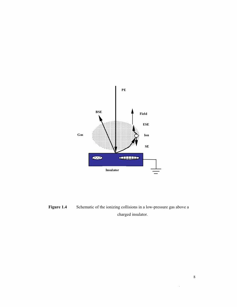
Figure 1.4 Schematic of the ionizing collisions in a low-pressure gas above a

charged insulator.

8

compensation. Charge carriers in the gas are PE, BSE, SE, ionized gas molecules,

electrons liberated as a consequence of ionizing collisions involving gas molecules (ESE)

and electrons liberated by positive ions impact on the sample surface (ESE). The major

contribution to the gas cascade comes from the SE emanating from the sample surface

due to their low energy [Toth et al. 2000]. On the other hand, the positive ions have a

much higher mass than electrons so that their mobility is lower than electron, and an ion-

gas collision is easier than an electron-gas collision. These two kinds of particles can

effectively neutralize the charging surface. All the factors above induce the gas ionization

avalanche, producing ion current, which takes charge of the charging neutralization. The

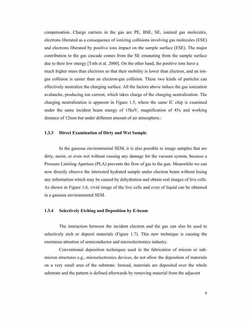
charging neutralization is apparent in Figure 1.5, where the same IC chip is examined

under the same incident beam energy of 15keV, magnification of 45x and working

distance of 12mm but under different amount of air atmosphere.:

1.3.3 Direct Examination of Dirty and Wet Sample

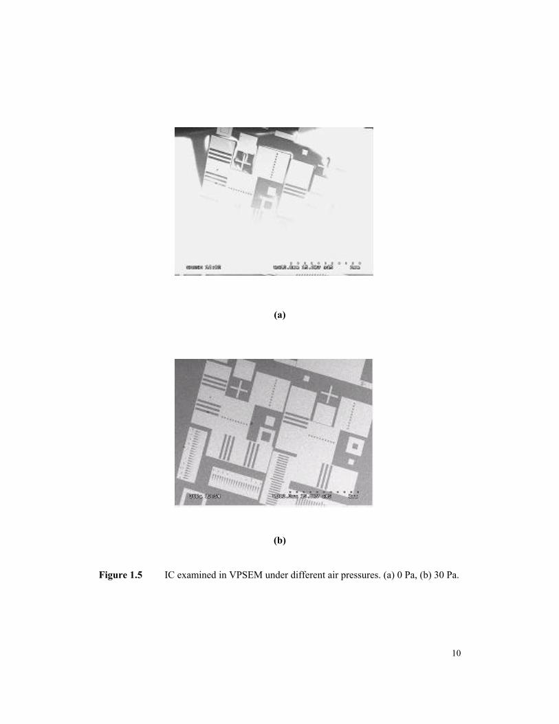
In the gaseous environmental SEM, it is also possible to image samples that are

dirty, moist, or even wet without causing any damage for the vacuum system, because a

Pressure Limiting Aperture (PLA) prevents the flow of gas to the gun. Meanwhile we can

now directly observe the interested hydrated sample under electron beam without losing

any information which may be caused by dehydration and obtain real images of live cells.

As shown in Figure 1.6, vivid image of the live cells and even of liquid can be obtained

in a gaseous environmental SEM.

1.3.4 Selectively Etching and Deposition by E-beam

The interaction between the incident electron and the gas can also be used to

selectively etch or deposit materials (Figure 1.7). This new technique is causing the

enormous attention of semiconductor and microelectronics industry.

Conventional deposition techniques used in the fabrication of micron or sub-

micron structures e.g., microelectronics devices, do not allow the deposition of materials

on a very small area of the substrate. Instead, materials are deposited over the whole

substrate and the pattern is defined afterwards by removing material from the adjacent

9

(a)

(b)

Figure 1.5 IC examined in VPSEM under different air pressures. (a) 0 Pa, (b) 30 Pa.

10

(a)

(b)

Figure 1.6 Live cells and liquid specimen examined in ESEM. (a) Spore, (b) Cell

water.

Source: http://www.feic.com/esem/gal4.html

11

.

(a)

(b)

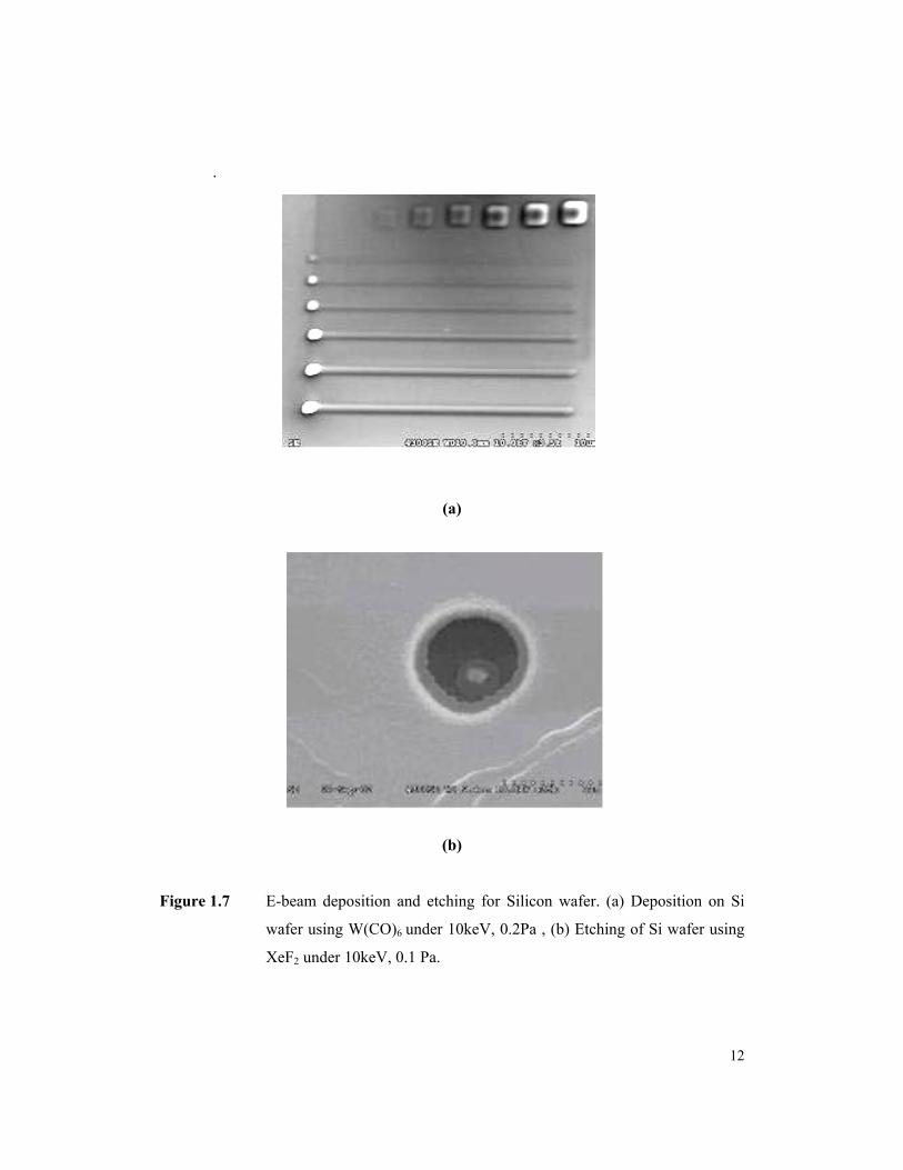
Figure 1.7 E-beam deposition and etching for Silicon wafer. (a) Deposition on Si

wafer using W(CO)6 under 10keV, 0.2Pa , (b) Etching of Si wafer using

XeF2 under 10keV, 0.1 Pa.

12

resists, photo- or electron-beam lithography, lift-off, and/or selective etching which result

in costly processes and generally require planar substrates [Folch 1996].

Electron beam deposition (EBD) is a novel method (Figure 1.7) for directly

applying the desired material on only a very small area of a substrate (selective

deposition) at low temperature. This represents an attractive application of electron beam

induced chemical reaction at a gas-substrate interface [Matsui 1986)]. In the presence of a

surrounding gas, a finely focused electron beam is observed to cause the deposition of

material from the gas only in the area irradiated by the beam. Nanometer structures can

be fabricated by electron beam induced surface reaction, because beam diameters, as

small as 0.5 nm, can be formed with conventional electron optical equipment [Broers

1976)]. In EBD, materials are patterned and deposited simultaneously, so it is an

inexpensive technique due to its maskless and resistless. The technique of EBD is

suitable for the fabrication of structures of different sizes, shapes, and materials in the

sub-micron or nanometer scale.

Directly etching is also possible by using the electron beam induced surface

reaction. Coburn et al. [1987] reported Si, SiO2 and Si3N4 etched by electron beam

induced reactions using an XeF2 gas source that Matsui [Matsui 1987] reports that W

deposition from WF6 took place at SiO2 substrate of temperature below 50ºC but etching

occurred when temperature higher than 50ºC.

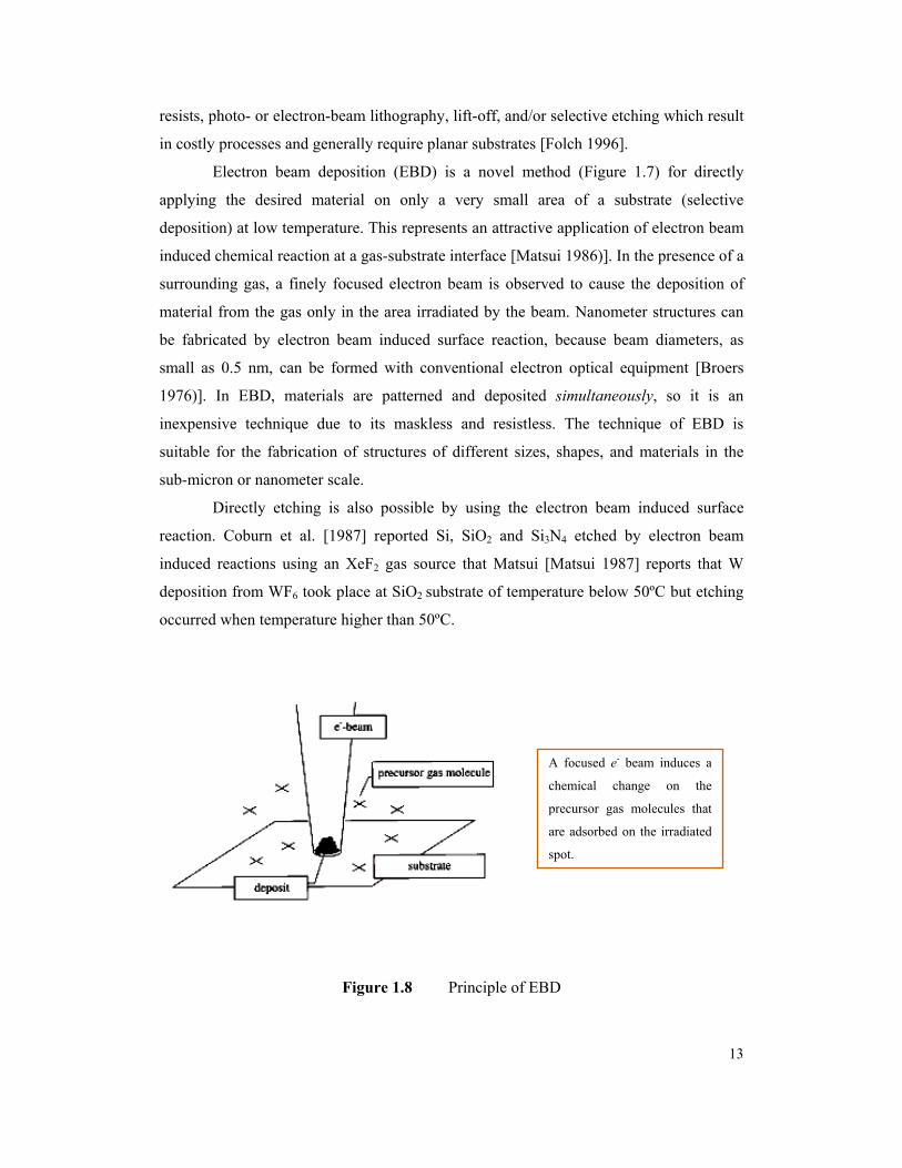
A focused e- beam induces a

chemical change on the

precursor gas molecules that

are adsorbed on the irradiated

spot.

Figure 1.8 Principle of EBD

13

The deposition rate depends on the total e-beam current density at the beam spot,

on the effective absorption rate of the precursor gas molecules onto the substrate, and on

the probability for an electron to cause EBD of a molecule. In addition, the beam current

density depends not only on the beam spot size but also on the rate of emission of

secondary and backscattered electrons, which also contribute to the process [Matsui

1989].

1.4 Electron Beam Scattering

For all of these reasons there is, therefore, growing interest in understanding the

problem of performing scanning microscopy in the presence of a low pressure of gas.

One of the most important problems is the fact that the electron beam is scattered by its

interactions with the gas.

1.4.1 Scattering Introduction

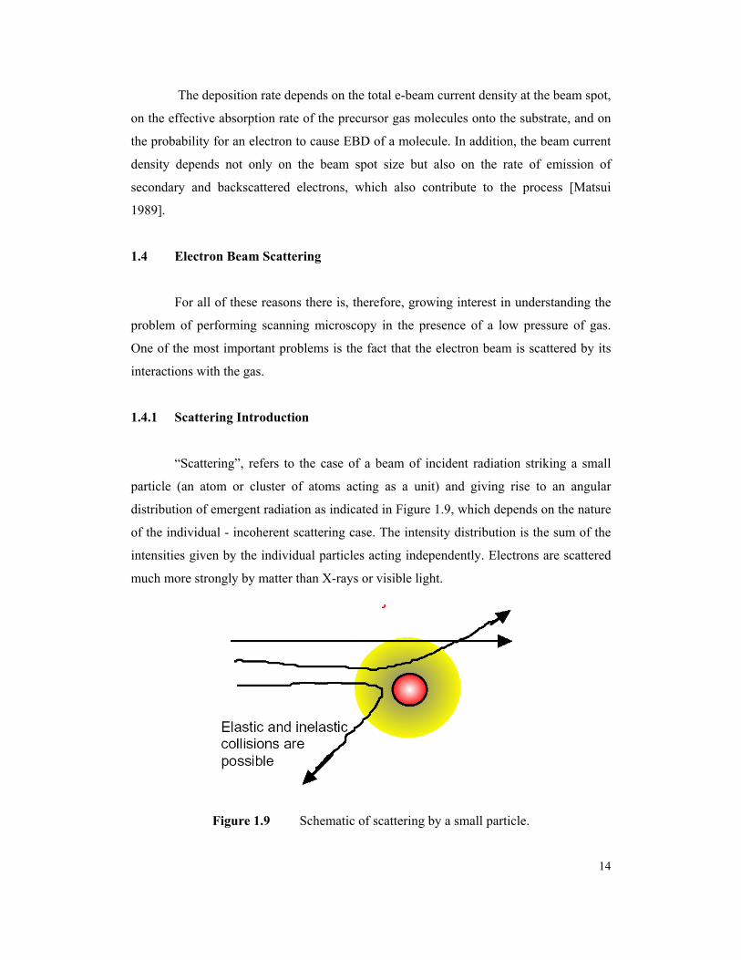
“Scattering”, refers to the case of a beam of incident radiation striking a small

particle (an atom or cluster of atoms acting as a unit) and giving rise to an angular

distribution of emergent radiation as indicated in Figure 1.9, which depends on the nature

of the individual - incoherent scattering case. The intensity distribution is the sum of the

intensities given by the individual particles acting independently. Electrons are scattered

much more strongly by matter than X-rays or visible light.

Figure 1.9 Schematic of scattering by a small particle.

14

Collisions between objects are governed by laws of momentum and energy.

When a collision occurs in an isolated system, the total momentum of the system of

objects is conserved. Provided that there are no net external forces acting upon the

objects, the momentum of all objects before the collision equals the momentum of all

objects after the collision. If there are only two objects involved in the collision, then the

momentum change of the individual objects are equal in magnitude and opposite in

direction.

Certain collisions are referred to as elastic collisions. Elastic collisions are

collisions in which both momentum and kinetic energy are conserved. The total system

kinetic energy before the collision equals the total system kinetic energy after the

collision. If total kinetic energy is not conserved, then the collision is referred to as an

inelastic collision.

1.4.2 Electron Beam Scattering by Gas

In SEM, when the electron beam strikes the specimen, there are a host of possible

reactions or interactions between the primary electron beam and the specimen, and their

study has constituted a fundamental topic of electron microscopy [Mathieu, 1999]. Thus,

a primary electron may undergo elastic or inelastic collisions in the specimen resulting in

the generation of secondary (SE) or backscattered electrons (BSE), X-rays etc., and

changes in the specimen by molecular scission or cross linking. All of these different

interactions are characterized by the fact that they occur between two entities: the beam

and the specimen.

By allowing gas around the specimen, the number and the type of reactions are

multiplied and it is helpful if these reactions are classified and studied in a logical manner

according to some natural distinction. Four main entities and be distinguished which

interact with each other: Beam, gas, specimen and signals [Danilatos 1990b]. Therefore

the large number of reactions can be subdivided into six general types of interactions.

These general types are not independent from each other and thy may influence each

other.

Beam-specimen interactions: result in (1) beam scattering, which determines the

interaction volume (2) generation of signals (3) modification of the nature of the

specimen (beam irradiation effects).

15

Beam-gas interactions: result in (a) scattering of the beam, (2) generation of

signals such as SE, BSE, X-rays and photons. (3) Modification of the gas due to the

creation of positive and negative ions, dissociation products and excited molecules.

Specimen-signal interactions: results primarily in signal modifications and, to a

minor extent, in specimen modification. One example for signals modified by the

specimen is that secondary electrons are modified by a charged surface, or BSE by

topographic undulations. Signal-gas interactions: results a mutual modification both of

the signal and the gas. This type of interaction is of extreme significance in the VPSEM

and is an important area of investigation. Gas-specimen interactions: are as expected

from the general physical-chemical reactions in studies outside electron microscopy.

Beam-signal interaction: beam can affect the signals indirectly through its interaction

with the gas (the background noise).

Among these interactions, beam-specimen and beam-gas interactions are most

important and most used interactions nowadays. Both these interactions could result in

scattering of electron beam, but one difference we should notice is that scattering due to

Beam-specimen interaction happens inside the sample, while the scattering due to Beam-

gas interaction take place before the electron beam impinge the specimen surface. There

are extensive established theories, computer simulations, and a significant literature on

beam-specimen interactions, so researchers have a clear concept of how the electrons

being scattered after their collision of the specimen. But the scattering of the primary

electron beam by the gas molecules is not well understood, so more beam-gas interaction

related theoretical and experimental studies are extremely necessary, especially this type

of interaction is causing more and more attentions because of the fast development of the

gases involved micro-scale production in the microelectronics and the semiconductor

industries. For this reason we concentrate on electron beam-gas scattering research in our

project.

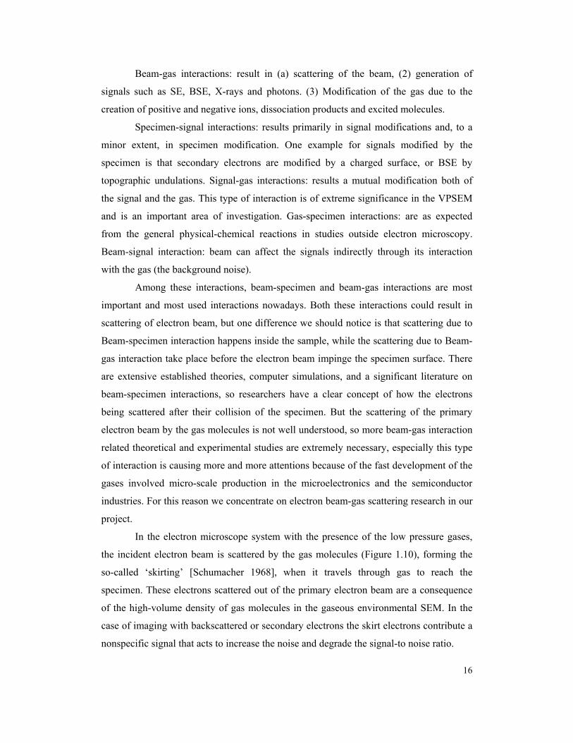
In the electron microscope system with the presence of the low pressure gases,

the incident electron beam is scattered by the gas molecules (Figure 1.10), forming the

so-called ‘skirting’ [Schumacher 1968], when it travels through gas to reach the

specimen. These electrons scattered out of the primary electron beam are a consequence

of the high-volume density of gas molecules in the gaseous environmental SEM. In the

case of imaging with backscattered or secondary electrons the skirt electrons contribute a

nonspecific signal that acts to increase the noise and degrade the signal-to noise ratio.

16

GPL

High VacuumPLA

Figure 1.10 Schematic of the scattering by surrounding gases in VPSEM.

17

Also a chemical characterization problem could arise when those X-rays generated by the

scattered electrons from a nearby material that is different in composition from the

interested material under the primary beam. Consequently the quality of the images of the

samples, or quality of the deposition, or etching during the micro processing, are all

directly limited by this factor, the scattering of the electron in the primary beam by the

gas [Stowe et al. 1998]. Therefore gas scattering of electrons must be considered here

while it has never been an issue in the conventional SEM.

Electron beam scattering is also classified as being elastic, when only negligible

electron energy transfer to the nucleus of the atom takes place, in the electron energy

range used in the SEM, or inelastic when the fast incident electron interacts with the

inner- or outer-shell atomic electrons [Egerton 1996] and lose relative large amount of

electron energy.

1.4.3 Gas Scattering Cross-section Introduction

It is necessary to understand qualitatively and quantitatively how the electron

beam is scattered so that we could accurately utilize the electron-gas interactions and

minimize the problems these interactions could cause. The amount of scattering of the

primary beam is dependent on a number of factors including electron beam cross-section,

working distance, gas pressure, gas composition, and accelerating voltage of the SEM

[Stowe et al. 1998].

The skirt electrons could contribute to a loss of contrast, beam current and so gas

scattering cross-section. For understanding how the electron beam scattered by presented

gas molecules, the gas scattering cross-sections is one of the most essential information

used to since it is a measurement for the magnitude of the electron beam scattering. It is a

paramount important parameter in electron beam study because this value makes it

possible to calculate the details of the electron distribution resulting from the collisions of

electrons with gas molecules or atoms. For example, the total cross-section can be used in

a suitable Monte Carlo simulation [Joy 1995, 1996] designed to simulate the spatial

distribution of the electrons striking the sample after passage through the gas.

1.4.3.1 Definition of Cross-section

18

When an incident beam traverses the target some of the particles may be

scattered from their original direction by interaction with the nuclei in the target. The

probability that an incident particle will undergo a specified type of interaction is

proportional to n, the number of target particles per unit area in the foil. If the probability

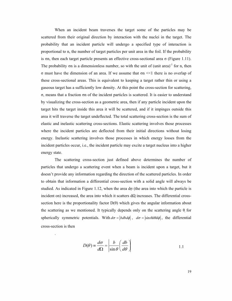
is σn, then each target particle presents an effective cross-sectional area σ (Figure 1.11).

The probability σn is a dimensionless number, so with the unit of (unit area)-1 for n, then

σ must have the dimension of an area. If we assume that σn <<1 there is no overlap of

these cross-sectional areas. This is equivalent to keeping a target rather thin or using a

gaseous target has a sufficiently low density. At this point the cross-section for scattering,

σ, means that a fraction σn of the incident particles is scattered. It is easier to understand

by visualizing the cross-section as a geometric area, then if any particle incident upon the

target hits the target inside this area it will be scattered, and if it impinges outside this

area it will traverse the target undeflected. The total scattering cross-section is the sum of

elastic and inelastic scattering cross-sections. Elastic scattering involves those processes

where the incident particles are deflected from their initial directions without losing

energy. Inelastic scattering involves those processes in which energy losses from the

incident particles occur, i.e., the incident particle may excite a target nucleus into a higher

energy state.

The scattering cross-section just defined above determines the number of

particles that undergo a scattering event when a beam is incident upon a target, but it

doesn’t provide any information regarding the direction of the scattered particles. In order

to obtain that information a differential cross-section with a solid angle will always be

studied. As indicated in Figure 1.12, when the area dσ (the area into which the particle is

incident on) increased, the area into which it scatters dΩ increases. The differential cross-

section here is the proportionality factor D(θ) which gives the angular information about

the scattering as we mentioned. It typically depends only on the scattering angle θ for

spherically symmetric potentials. With φσ bdbdd = , φθθσ ddd sin= , the differential

cross-section is then

.

=

Ω≡

θθσ

θddbb

ddD

sin)( 1.1

19

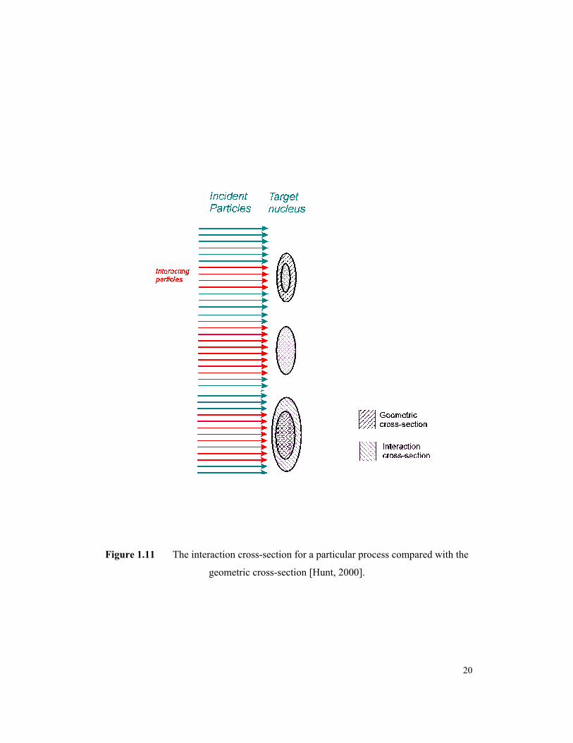
Figure 1.11 The interaction cross-section for a particular process compared with the

geometric cross-section [Hunt, 2000].

20

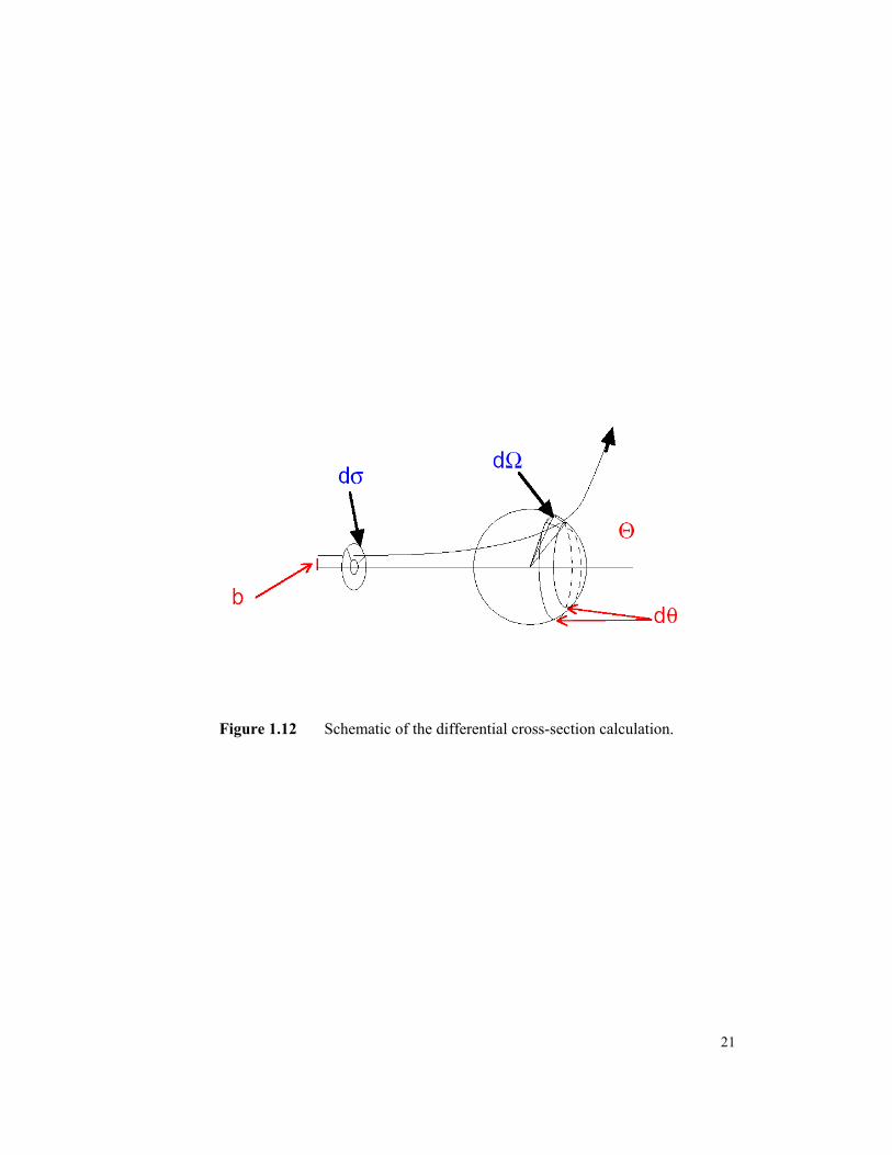
Figure 1.12 Schematic of the differential cross-section calculation.

21

The cross-section is a measure of the probability of an event, therefore it is not a

real area with a well-defined boundary and it may not bear any close relationship with the

physical size of atom cross-sectional area, which is approximately in the order of 10-16

cm2. In electron microscopy, the cross-section of most processes is much smaller than the

physical cross-section of atom. For example, the inner shell ionization cross-section is

typically in the range of 10-22~10-24cm2, and the total gas scattering cross-section studied

in this paper, is at the order of 10-18, 10-19 cm2. So, it is sometimes referred to as the

effective “size” which the atom or molecule presents as a target to the incident particle

because it has the dimension of an area.

The full dimensionality of the cross-section for the scattering of electrons by

atoms or molecules can be written as: Q (events/cm3)/[(e-/cm2)(atom/cm3)] [Goldstein et

al. 1992]. The cross-section is associated not only with electron scattering through a

given angle but also with other types of reaction such as ionization, excitation,

dissociation, molecular rotation, vibration, etc. Each possible interaction j is characterized

by a cross-section σj, the sum of which is also the total cross-section σT [Danilatos 1988].

1.4.3.2 Rutherford and Mott Cross-section

From the macroscopic point of view, the majority of the incident electrons are

considered as undergoing elastic scattering because the deflection from the inelastic

scattering is so small (<<1°) that it can be ignored. So the elastic cross-section has always

been the focus of study. Rutherford scattering is the elastic scattering produced by the

Coulomb force. It happens when the incident electron is attracted by the positive charge

in the nucleus, thus this scattering is often used to explore the shape of the nuclear

charge,

The Rutherford elastic cross-section is widely used in various calculations

because it gives analytical expression to compute θ, the angle of collision and λ, the

distance between collisions (mean free path). There are several points to notice about the

Rutherford scattering cross-section:

(a) It decreases rapidly with increasing angle θ;

(b) It becomes infinite at θ = 0;

(c) This cross-section inversely proportional to E2 (kinetic E) and

(d) It is proportional to (Qtarget* Qincident)2.

22

When the energy of the primary electrons is low or when the atomic number of

the target is high, the Rutherford elastic cross-sections are inaccurate because this theory

has been derived in the frame of the first Born approximation [Gauvin 1993]. In such

case, Mott cross-section is more appropriate to use.

1.4.3.3 Mean Free Path (MFP)

An important parameter related with the cross-section is the Mean Free Path λi

mentioned above. It can be defined as: the average distance traveled by a molecule

between collisions. It can be shown that the Mean Free Path is given by Eq. 1.2 with

given molecular diameter, d:

212dnπ

λ = 1.2

As expected, there is an inverse relationship between the number density of the molecules

(indicated by gas pressure) and the mean free path.

An electron with energy in the 5 – 2000 eV range passing through a solid can

lose energy via a number of processes. Neglecting the minimal energy loss that occurs

due to the excitation of phonons, there are three key processes: the electron-electron

scattering processes, the excitation of a valence and excitation of Auger electrons. The

net effect of these processes is that the Mean Free Path of an electron in a solid is

strongly dependent on its kinetic energy.

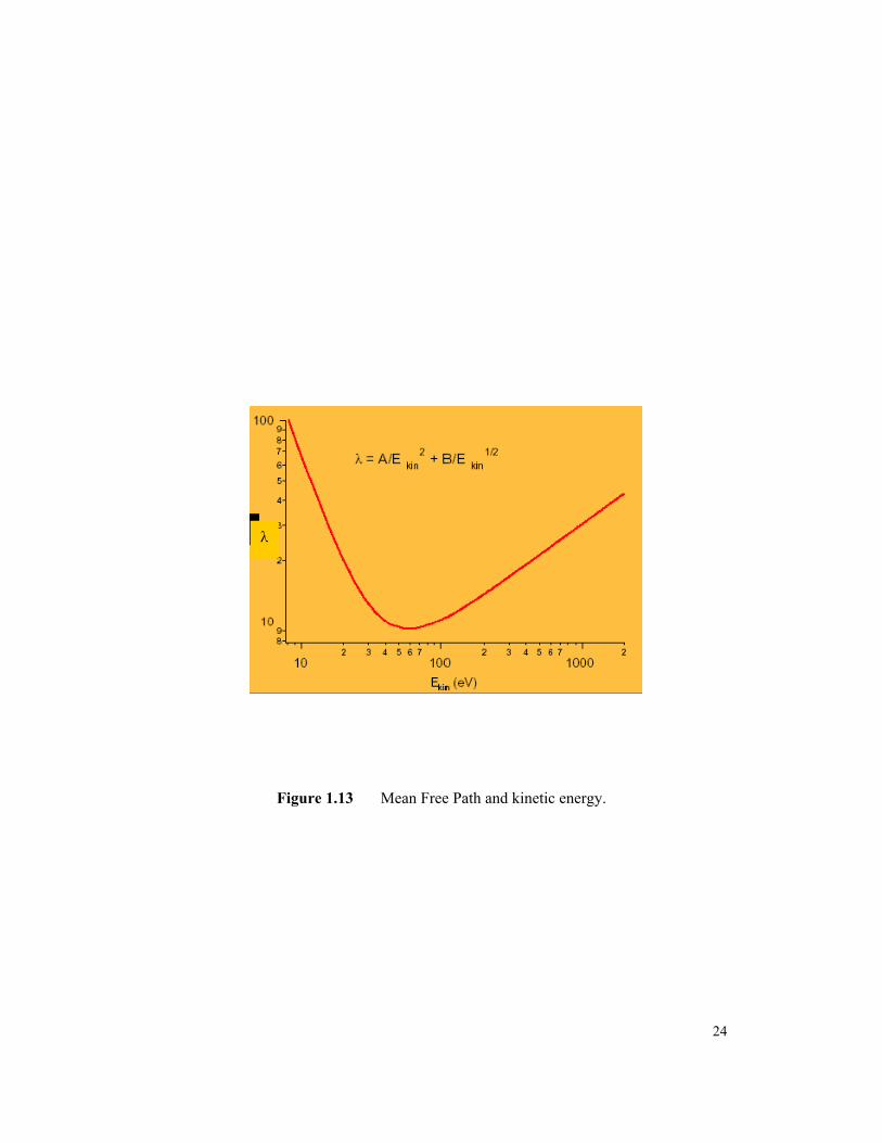
A schematic plot of the variation in electron Mean Free Path as a function of

electron kinetic energy is shown in Figure 1.13. This plot is usually referred to as the

"universal" Mean Free Path and loosely holds for electrons traveling through a very wide

range of materials. At very low kinetic energies the electron does not have enough energy

to excite either of the listed processes, so its Mean Free Path is long. At high kinetic

energies the electron spends less time passing through a solid, thus less likely to suffer

from an energy loss and its Mean Free Path becomes quite long. The Mean Free Path

passes through a minimum value between these two energy regions. The key process

determining the minimum in the Mean Free Path is actually the energy loss due to

plasmon excitation.

23

λ

Figure 1.13 Mean Free Path and kinetic energy.

24

CHAPTER II

DIRECTLY MEASUREMENT OF THE ELECTRON BEAM SCATTERING

2.1 Introduction

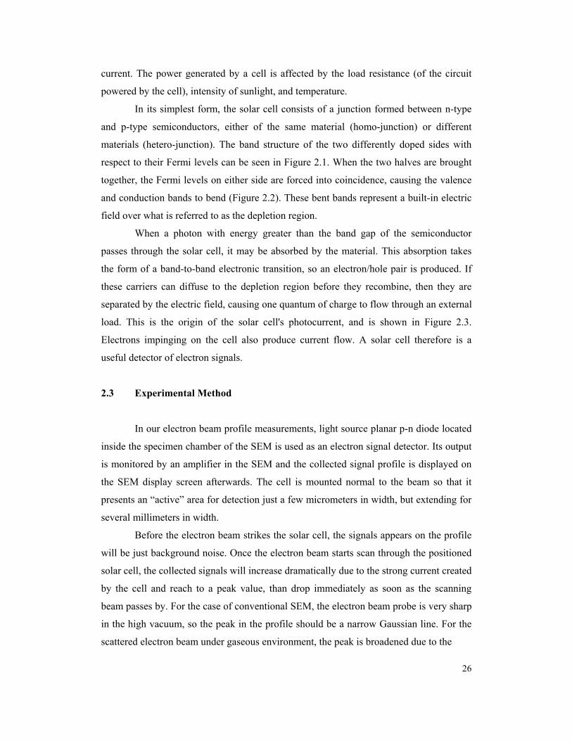
As discussed in chapter I that the quality of the images of the samples, quality of

the deposition, or etching during the micro processing, are all directly limited by electron

scattering in the primary beam by the gas, therefore the scattering of electron which is not

an issue in the conventional SEM, must be considered in the gaseous environmental

SEM. The scattering effect was predicted by Danilatos [1988] originally and has been

observed or measured by many researchers [Wight 1998, Gillen et al. 1998].

However, most of these experimental measurements and modeling are of limited

value. There are many possible uncertainties associated with these second-hand-

approaches because of the issues of X-rays production, absorption, geometry and

collection efficiency etc [Wight 1999], which could result in the reduction on the

accuracy of the study. Therefore the direct measurement of the distribution of the primary

electron beam and scattered electron beam would be important if it was available. But the

fact is that it is not easy to achieve because the extremely small size of the electron beam

and the environment it usually works under. One method using phosphor imaging plates

to directly measure the beam scattering has been introduced by Wight [1999].

We discuss here an alternative method in which a planar solar cell is used as an

electron signal detector to determine the beam profile.

2.2 Introduction of P-N Junction Solar Cell

Solar cells were initially introduced as a global energy source without air

pollution. Faced with ever-increasing demand, the earth's sources of non-renewable

energy are not expected to last long. Among the many contenders vying to replace fossil

fuels, photovoltaic solar cells offer many advantages, including needing little

maintenance and being relatively "environmentally-friendly". A solar cell is a

semiconductor device that converts light energy directly into electricity. For example, a

typical 2x4cm silicon solar cell produces 0.45 volts and up to 0.275 amps or so of usable

25

current. The power generated by a cell is affected by the load resistance (of the circuit

powered by the cell), intensity of sunlight, and temperature.

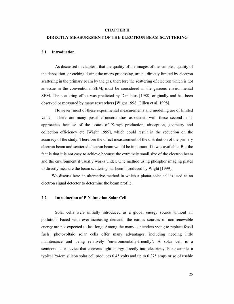
In its simplest form, the solar cell consists of a junction formed between n-type

and p-type semiconductors, either of the same material (homo-junction) or different

materials (hetero-junction). The band structure of the two differently doped sides with

respect to their Fermi levels can be seen in Figure 2.1. When the two halves are brought

together, the Fermi levels on either side are forced into coincidence, causing the valence

and conduction bands to bend (Figure 2.2). These bent bands represent a built-in electric

field over what is referred to as the depletion region.

When a photon with energy greater than the band gap of the semiconductor

passes through the solar cell, it may be absorbed by the material. This absorption takes

the form of a band-to-band electronic transition, so an electron/hole pair is produced. If

these carriers can diffuse to the depletion region before they recombine, then they are

separated by the electric field, causing one quantum of charge to flow through an external

load. This is the origin of the solar cell's photocurrent, and is shown in Figure 2.3.

Electrons impinging on the cell also produce current flow. A solar cell therefore is a

useful detector of electron signals.

2.3 Experimental Method

In our electron beam profile measurements, light source planar p-n diode located

inside the specimen chamber of the SEM is used as an electron signal detector. Its output

is monitored by an amplifier in the SEM and the collected signal profile is displayed on

the SEM display screen afterwards. The cell is mounted normal to the beam so that it

presents an “active” area for detection just a few micrometers in width, but extending for

several millimeters in width.

Before the electron beam strikes the solar cell, the signals appears on the profile

will be just background noise. Once the electron beam starts scan through the positioned

solar cell, the collected signals will increase dramatically due to the strong current created

by the cell and reach to a peak value, than drop immediately as soon as the scanning

beam passes by. For the case of conventional SEM, the electron beam probe is very sharp

in the high vacuum, so the peak in the profile should be a narrow Gaussian line. For the

scattered electron beam under gaseous environment, the peak is broadened due to the

26

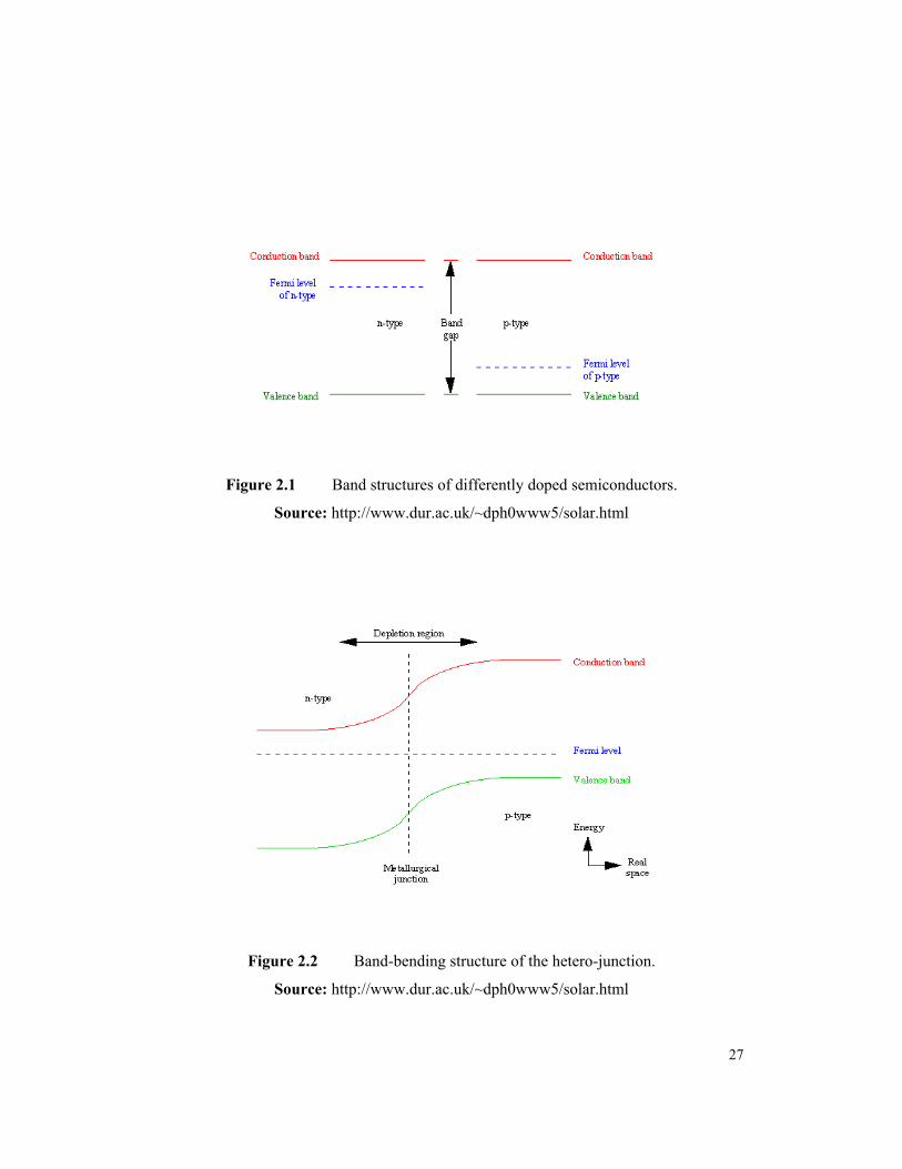
Figure 2.1 Band structures of differently doped semiconductors.

Source: http://www.dur.ac.uk/~dph0www5/solar.html

Figure 2.2 Band-bending structure of the hetero-junction.

Source: http://www.dur.ac.uk/~dph0www5/solar.html

27

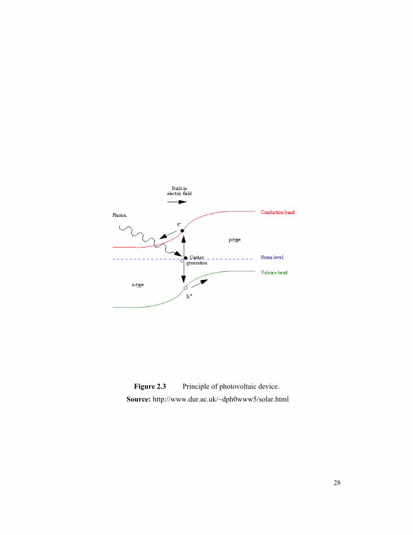
Figure 2.3 Principle of photovoltaic device.

Source: http://www.dur.ac.uk/~dph0www5/solar.html

28

scattering, and the broadening under various experimental variables, such as accelerating

voltage of the electron beam gas pressure, gas composition beam gas path length etc that

are the direct measurements of our interests.

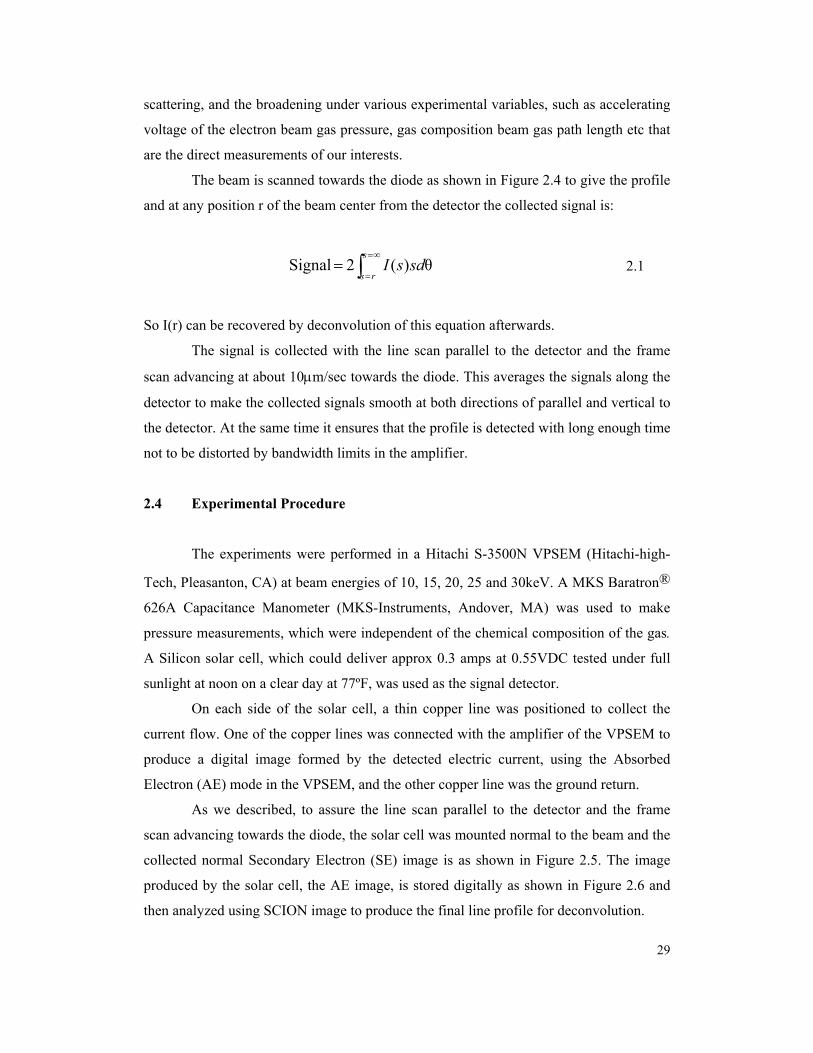
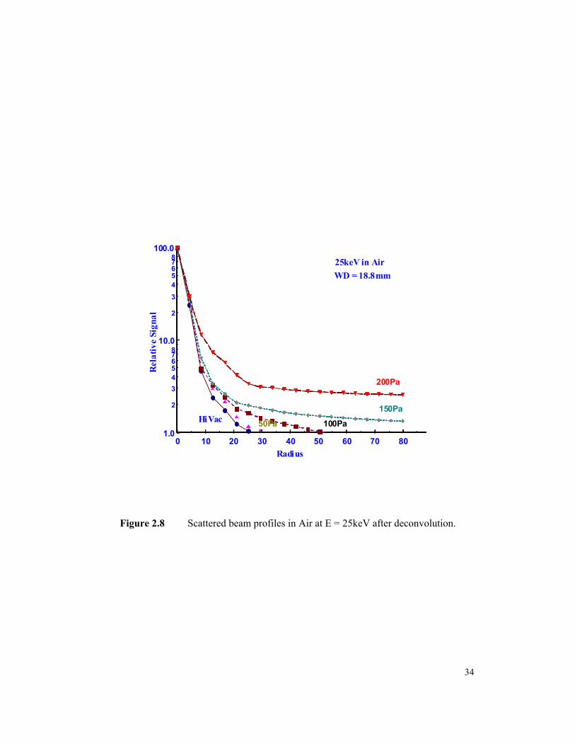
The beam is scanned towards the diode as shown in Figure 2.4 to give the profile

and at any position r of the beam center from the detector the collected signal is:

∫∞=

==

s

rssdsI θ)(2 Signal 2.1

So I(r) can be recovered by deconvolution of this equation afterwards.

The signal is collected with the line scan parallel to the detector and the frame

scan advancing at about 10µm/sec towards the diode. This averages the signals along the

detector to make the collected signals smooth at both directions of parallel and vertical to

the detector. At the same time it ensures that the profile is detected with long enough time

not to be distorted by bandwidth limits in the amplifier.

2.4 Experimental Procedure

The experiments were performed in a Hitachi S-3500N VPSEM (Hitachi-high-

Tech, Pleasanton, CA) at beam energies of 10, 15, 20, 25 and 30keV. A MKS Baratron®

626A Capacitance Manometer (MKS-Instruments, Andover, MA) was used to make

pressure measurements, which were independent of the chemical composition of the gas.

A Silicon solar cell, which could deliver approx 0.3 amps at 0.55VDC tested under full

sunlight at noon on a clear day at 77ºF, was used as the signal detector.

On each side of the solar cell, a thin copper line was positioned to collect the

current flow. One of the copper lines was connected with the amplifier of the VPSEM to

produce a digital image formed by the detected electric current, using the Absorbed

Electron (AE) mode in the VPSEM, and the other copper line was the ground return.

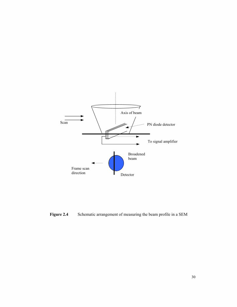
As we described, to assure the line scan parallel to the detector and the frame

scan advancing towards the diode, the solar cell was mounted normal to the beam and the

collected normal Secondary Electron (SE) image is as shown in Figure 2.5. The image

produced by the solar cell, the AE image, is stored digitally as shown in Figure 2.6 and

then analyzed using SCION image to produce the final line profile for deconvolution.

29

Broadened beam

Detector Frame scan direction

Axis of beam

Scan PN diode detector

To signal amplifier

Figure 2.4 Schematic arrangement of measuring the beam profile in a SEM

30

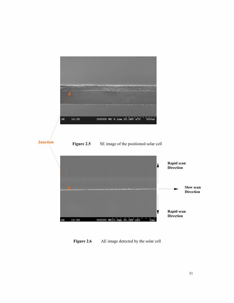
Figure 2.5 SE image of the positioned solar cell

Junction

Rapid scan Direction

Rapid scan Direction

Slow scan Direction

Figure 2.6 AE image detected by the solar cell

31

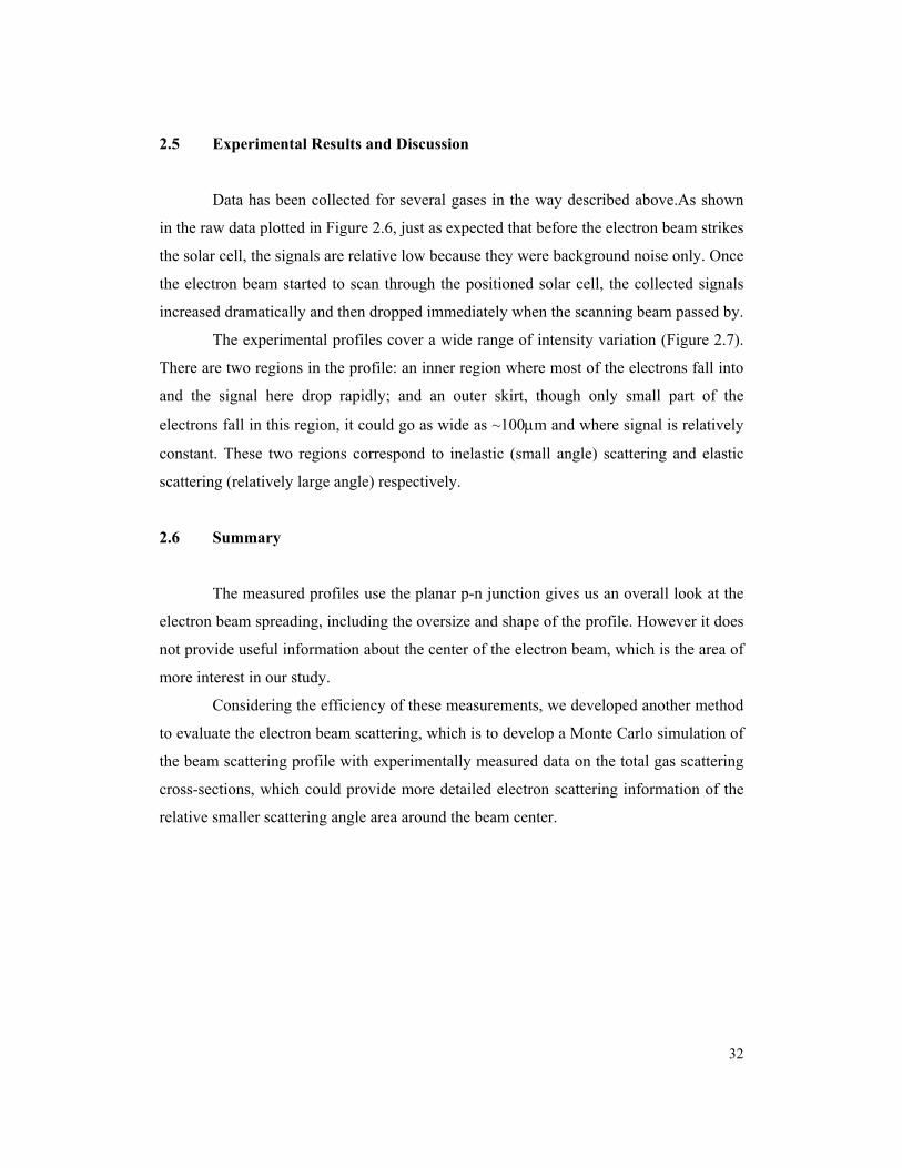
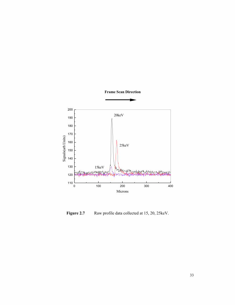
2.5 Experimental Results and Discussion

Data has been collected for several gases in the way described above.As shown

in the raw data plotted in Figure 2.6, just as expected that before the electron beam strikes

the solar cell, the signals are relative low because they were background noise only. Once

the electron beam started to scan through the positioned solar cell, the collected signals

increased dramatically and then dropped immediately when the scanning beam passed by.

The experimental profiles cover a wide range of intensity variation (Figure 2.7).

There are two regions in the profile: an inner region where most of the electrons fall into

and the signal here drop rapidly; and an outer skirt, though only small part of the

electrons fall in this region, it could go as wide as ~100µm and where signal is relatively

constant. These two regions correspond to inelastic (small angle) scattering and elastic

scattering (relatively large angle) respectively.

2.6 Summary

The measured profiles use the planar p-n junction gives us an overall look at the

electron beam spreading, including the oversize and shape of the profile. However it does

not provide useful information about the center of the electron beam, which is the area of

more interest in our study.

Considering the efficiency of these measurements, we developed another method

to evaluate the electron beam scattering, which is to develop a Monte Carlo simulation of

the beam scattering profile with experimentally measured data on the total gas scattering

cross-sections, which could provide more detailed electron scattering information of the

relative smaller scattering angle area around the beam center.

32

Frame Scan Direction

0 100 200 300 400110

120

130

140

150

160

170

180

190

200

20keV

15keV

25keV

Sign

als(

arb.

Uni

ts)

Microns

Figure 2.7 Raw profile data collected at 15, 20, 25keV.

33

0 10 20 30 40 50 60 70 80 Radius

1.0

10.0

100.0

2 3 4 5 6 7 8

2 3 4 5 6 7 8

Rel

ativ

e Si

gnal

150Pa100PaHiVac

WD = 18.8mm 25keV in Air

200Pa

50Pa

Figure 2.8 Scattered beam profiles in Air at E = 25keV after deconvolution.

34

CHAPTER III

MEASUREMENT OF TOTAL GAS SCATTERING CROSS-SECTION

3.1 Introduction

The total gas scattering cross-sections data is one of the essential information

required for developing a Monte Carlo simulation of the beam scattering. However there

seems considerable difficulty in establishing a universal theory of scattering cross-

sections for all gases that can be confirmed by experiment. Relatively few total gas

scattering cross-sections are available for the conditions of gas pressure, and electron

beam energy that are of interest in the electron microscopy field. Cross-section values are

not easy to compute because the vibrational modes of the gas molecules add an additional

contribution to the value of the scattering cross-section, and they are also difficult to

predict unless the atomicity (i.e. effective atom cluster size [Ditmire 1997]) of the

molecule of gas is known. Since the experimental data available on cross-sections are

definitely inadequate and because there is also insufficient experimental verification for

the theoretically calculated cross-sections in current use, systematic experimental

measurements of the total gas scattering cross-sections presented are necessary.

In our project, the total gas scattering cross-section was experimentally measured

using the technique of Gauvin [Gauvin et al. 1999]. This method depends on an

observation of the variation of the fluorescent X-ray intensity excited by the electron

beam with variable gas pressure from a small target. The advantage of this technique is

that the variation of X-ray intensity with pressure will be due only to the decrease of the

on-axis intensity of the unscattered beam with pressure, since the scattered part of the

beam goes into the skirt region of the beam and hence misses the particle, so reducing the

signal collected by X-ray detector. The effect caused by any ions generated from

secondary electrons on the current measuring by the Faraday cup is eliminated here since

it is only the characteristic X-ray intensity of the specified spot on specimen that is

measured.

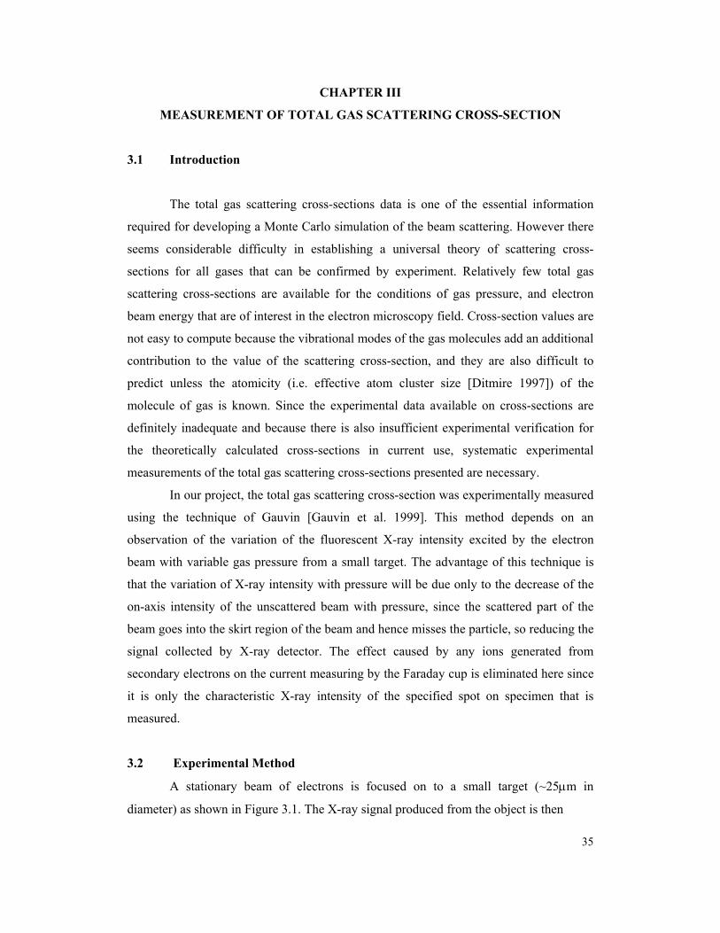
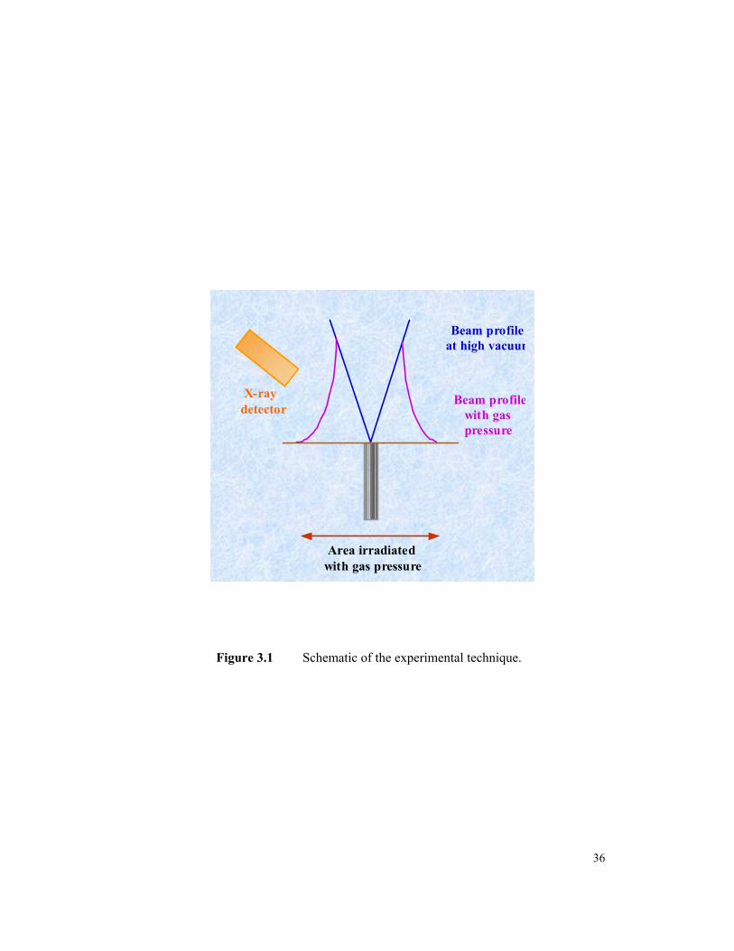
3.2 Experimental Method

A stationary beam of electrons is focused on to a small target (~25µm in

diameter) as shown in Figure 3.1. The X-ray signal produced from the object is then

35

Area irradiatedwith gas pressure

Beam profile at high vacuum

X-ray detector

Beam profilewith gas pressure

Figure 3.1 Schematic of the experimental technique.

36

measured as a function of the gas pressure. As the pressure increases electrons are

scattered into the skirt and so miss the object and the X-ray signal falls.

The total scattering cross-section of gas can then be calculated by an equation

derived from the expected Poisson distribution of the scattered electrons and the Gas Law

as [Gauvin et al. 2000]:

)ln()ln( 0IPRT

DI T +−=

σ 3.1

where I is the measured X-ray intensity at a given pressure P, σT is the total elastic cross-

section of the gas at certain energy of electron beam, D is the gas path length (i.e. the

average distance traveled by an incident electron from the position where it leaves the

high vacuum region of the VPSEM to the point where it reaches the sample surface), R is

the perfect gas constant and T is the temperature in degree Kelvin. With the slope, α

obtained from the linear relationship between loge(I) and P identified by Eq.3.1, the total

scattering cross-section can then be easily deduced as indicated in Eq.3.2:

DRT

Tασ −= 3.2

The cross-section determined in this way will include all elastic and inelastic

events which scatter the incident electron through and angle φ > ρ/D, where ρ is the

diameter of the target, here φ is about 2 milliradians.

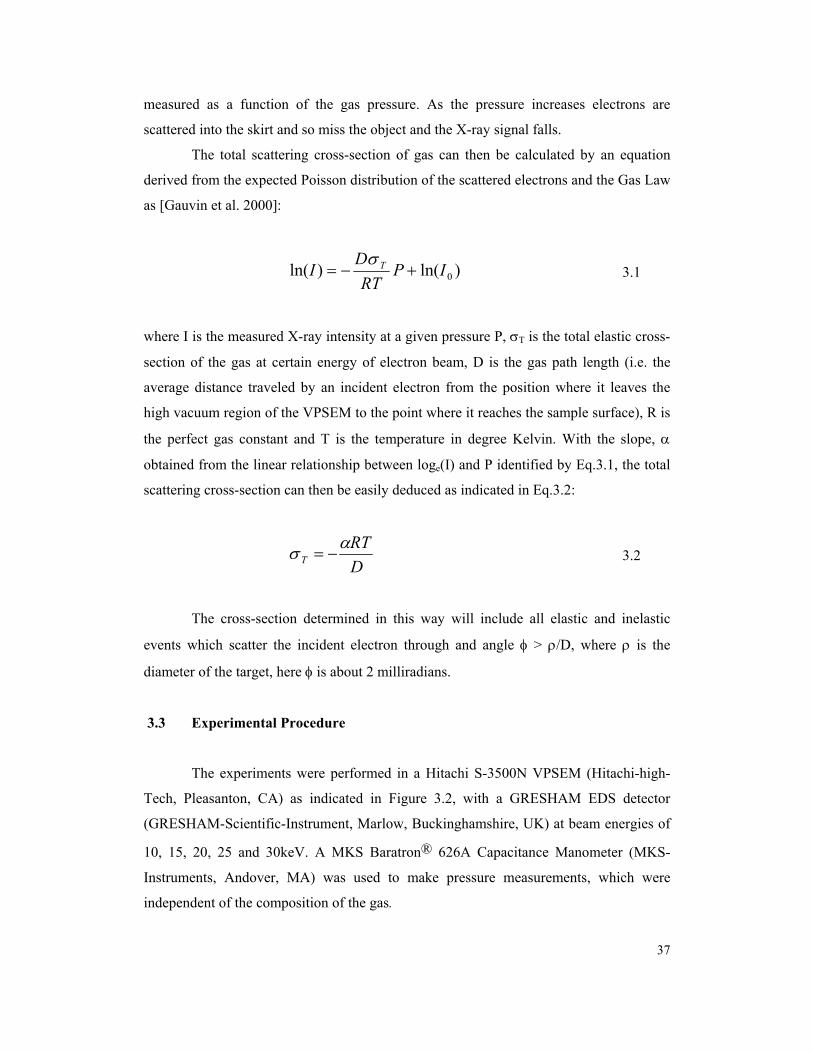
3.3 Experimental Procedure

The experiments were performed in a Hitachi S-3500N VPSEM (Hitachi-high-

Tech, Pleasanton, CA) as indicated in Figure 3.2, with a GRESHAM EDS detector

(GRESHAM-Scientific-Instrument, Marlow, Buckinghamshire, UK) at beam energies of

10, 15, 20, 25 and 30keV. A MKS Baratron® 626A Capacitance Manometer (MKS-

Instruments, Andover, MA) was used to make pressure measurements, which were

independent of the composition of the gas.

37

Figure 3.2 Experimental equipment (VPSEM, EDS, Manometer).

38

In order to optimize the collection of the X-ray emission the specimen was held

at the standard X-ray position corresponding to a gas path length of 12 mm, and the

magnification was x18K. The X-ray intensity was obtained by collecting the X-ray

signals emitted by the surface of a fine aluminum wire of 25 µm diameter inlaid in epoxy

resin (Figure 3.3). To avoid charging build up resulting from the use of a nonconductive

resin, the specimen was coated with a thin layer of gold-palladium. The selected

fluorescent X-ray peak in this experiment was Al kα whose characteristic energy is 1.5

keV and the counting time (i.e. live time) was 300 seconds. For the chosen beam energy

data was then recorded as the pressure was raised from below 1 Pa to its maximum value,

typically 270Pa. A second run of data was recorded as the pressure was reduced back to

1Pa. This was done to ensure efficient mixing of the gas of interest as discussed below.

The gas was introduced into the chamber through the computer controlled inlet needle

valve. A small container of the gas of interest, at a pressure just slightly above

atmospheric, was connected directly to the intake nozzle by a short piece of tubing.

3.4 Experimental Results

3.4.1 Linear Relationship of Ln (I) and P

As demonstrated above Gauvin’s technique suggests a linear relationship

variation of ln (Ip/I0) with Pressure, and as seen in Figure 3.4 through Figure 3.8, this

prediction is experimentally obeyed very well over a wide range of gas species and

incident beam energies, which indicates that the established basic model is correct. These

plots shown clearly illustrate how different gases scatter electrons by different amounts.

The data points plotted are the average of the values obtained as the pressure is first

increased to 300 Pa and then decreased back to 0 Pa.

3.4.2 Calculated Total Scattering Cross-sections

From these plots, the total gas scattering cross-section can be easily derived from

the slope of the data line at each energy as discussed in Eq 3.1, 3.2.

For multiple sets of raw data obtained in different time period for gases, statistic

models were fit to all sets of data points to test the variablilities over different trials:

39

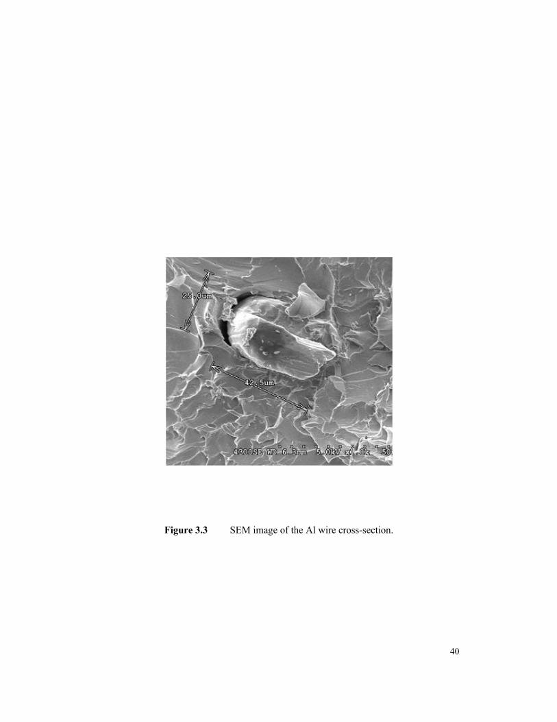
Figure 3.3 SEM image of the Al wire cross-section.

40

7

8

9

10

11

12

13

14

0 20 40 60 80 100 120 140 160 180Pressure(Pa)

ln(c

ount

s)

10kv 15kv20kv 25kv30kv

Air

Figure 3.4 Linear relationship of ln (I) and P for Air.

41

10

11

12

13

14

15

0 20 40 60 80 100 120 140 160 180

Pressure(Pa)

ln(c

ount

s)

10kv 15kv20kv 25kv30kv

He

Figure 3.5 Linear relationship of ln (I) and P for Helium.

42

Argon

11.5

12.0

12.5

13.0

13.5

14.0

14.5

0 20 40 60 80 100 120 140 160Pressure(Pa)

ln(c

ount

s)

15kv 20kv30kv 25kv

Figure 3.6 Linear relationship of ln (I) and P for Argon.

43

CH4

10.5

11.0

11.5

12.0

12.5

13.0

13.5

0 20 40 60 80 1

Pressure(Pa)

ln(c

ount

s)

00

10kv 15kv20kv 25kv30kv

Figure 3.7 Linear relationship of ln (I) and P for Methane.

44

9

10

11

12

13

14

15

0 50 100 150 200 250 300

Pressure (Pa)

ln (C

ount

s)

Air

HeArgon

CH4

Figure 3.8 Linear relationship of ln (I) and P for gases at 15keV.

45

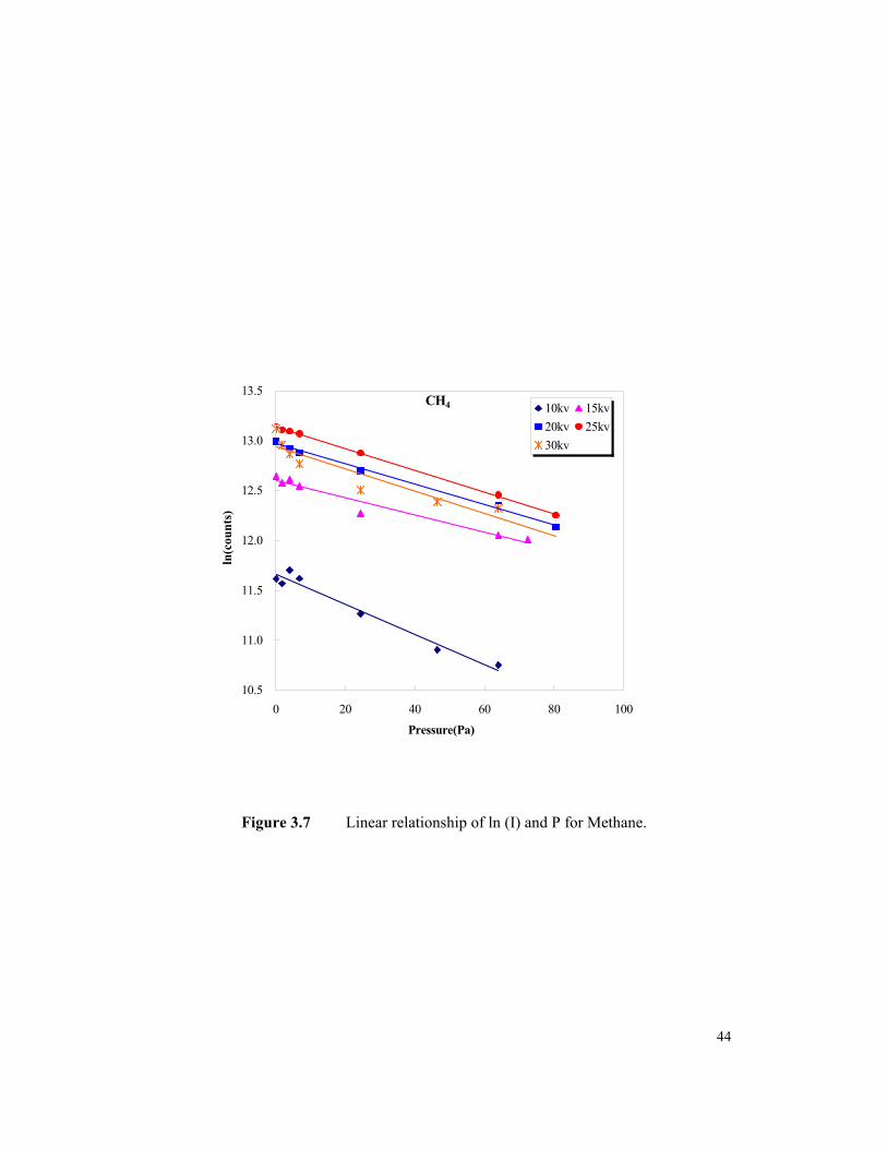
• If the factor Pressure*Trial is statistically nonsignificant at level of 0.01 in the

tests, it suggests that the variability due to different trials are nonsignificant.

Therefore the final regression line for that beam energy was deduced based on all

sets of data without the Pressure*Trial term in the model. With the slope of the

regression line, the cross-section (σ) value with its standard error (SE) can be

easily calculated.

• If factor Pressure*Trial is statistically significant at level of 0.01, it means that

the variability caused by different trials can not be ignored. A model was

constructed considering the Trial as random effect, and the regression line was

fitted to the model using REML (REstricted or REsidual Maximum Likelihood)

[Montgomery, 2000] approach. With the slope deduced from the regression line,

the cross-section (σ) value with its standard error (SE) was then calculated.

Based on the method described above, the obtained total gas scattering cross-

sections of air with the theoretical Mott’s cross-sections of air are listed in Table 3.1. For

higher beam energy, the stronger linear relationship between the ln (I) and air pressure,

which result in larger scattering cross-section. The reason is at higher beam energy,

electron beam is less likely scattered, so more emitted Alkα signals can be collected. The

difference between the experimental calculated cross-section of air and Mott’s cross-

sections for air is also noticeable. One possible reason suggested by the data is that in this

pressure regime most gas molecules are aggregated in clusters. Another reason is that

Mott’s cross-section only accounts for a part of the total scattering event - the elastic

scattering.

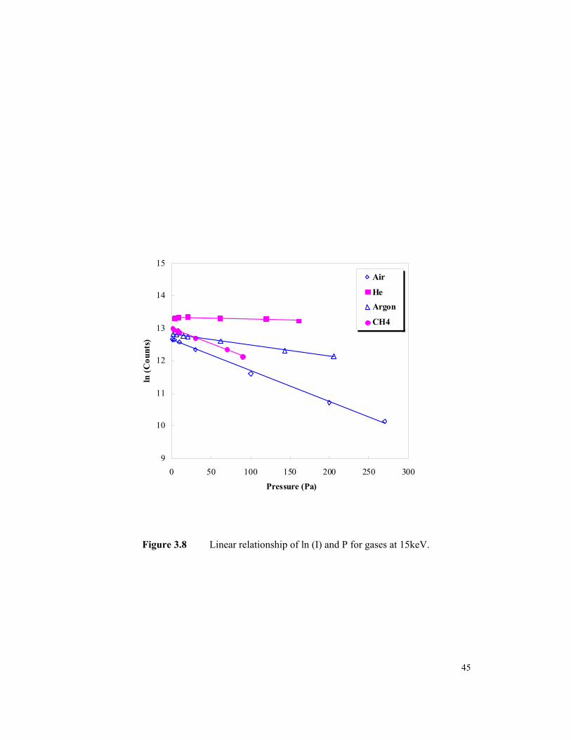
The calculated total scattering cross-sections of other investigated gases are also

tabulated below (Table 3.2) in units of cm2/atom. As anticipated helium scatters the least

strongly (i.e. has the lowest cross-section) while air scatters the most strongly (i.e. highest

cross-section), the difference being about a factor of 10 times. As the beam energy rises

the scattering cross-section would be expected to fall, as is observed for air and helium.

The somewhat anomalous behavior of the argon and methane data, in which the cross-

section between 20keV and 30keV remain essentially constant with beam energy, may be

the result of less than perfect mixing of the gas in the specimen chamber, or of statistical

or of uncorrected errors in the procedure.

46

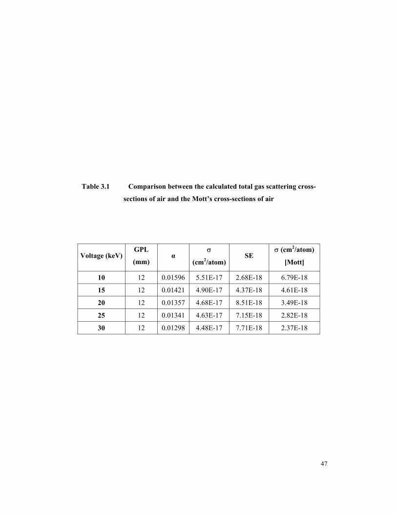
Table 3.1 Comparison between the calculated total gas scattering cross-

sections of air and the Mott’s cross-sections of air

Voltage (keV) GPL

(mm) α

σ

(cm2/atom) SE

σ (cm2/atom)

[Mott]

10 12 0.01596 5.51E-17 2.68E-18 6.79E-18

15 12 0.01421 4.90E-17 4.37E-18 4.61E-18

20 12 0.01357 4.68E-17 8.51E-18 3.49E-18

25 12 0.01341 4.63E-17 7.15E-18 2.82E-18

30 12 0.01298 4.48E-17 7.71E-18 2.37E-18

47

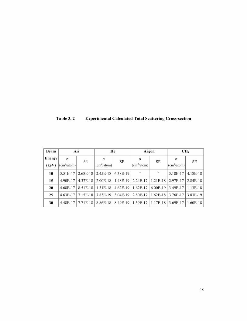
Table 3. 2 Experimental Calculated Total Scattering Cross-section

Air He Argon CH4 Beam

Energy

(keV) σ

(cm2/atom) SE

σ

(cm2/atom) SE

σ

(cm2/atom) SE

σ

(cm2/atom) SE

10 5.51E-17 2.68E-18 2.45E-18 6.38E-19 - - 5.18E-17 4.18E-18

15 4.90E-17 4.37E-18 2.00E-18 1.48E-19 2.24E-17 1.21E-18 2.97E-17 2.84E-18

20 4.68E-17 8.51E-18 1.31E-18 4.62E-19 1.62E-17 6.00E-19 3.49E-17 1.13E-18

25 4.63E-17 7.15E-18 7.83E-19 3.04E-19 2.80E-17 1.62E-18 3.76E-17 3.83E-19

30 4.48E-17 7.71E-18 8.86E-18 8.49E-19 1.59E-17 1.17E-18 3.69E-17 1.60E-18

48

3.5 Discussion of Errors in the Procedure

Before comparing the experimental total scattering cross-sections with theoretical

values, there are several key factors in this experimental procedure which need to be

discussed, first to assess the accuracy and precision of this work: the measurement of gas

pressure, the determination of the gas path length (GPL), and the alteration of the gas

temperatures inside the specimen chamber.

3.5.1 Gas Pressure Measurement in the VPSEM

In an environmental or VPSEM, the pressure is controlled by a computer

operated leak valve and a suitable feedback circuit monitoring the pressure read by a

Pirani gauge. Typically this leads to a condition in which the pressure cycles slowly with

time about the nominal value as the valve opens and closes, and results in the difficulty of

the correct determination of the gas pressure. Furthermore, on our instrument the gauge is

positioned very close to the inlet valve and therefore reads a pressure which may not be

truly representative of the true chamber vacuum. Finally, the reading of the Pirani gauge

is strongly dependent on the chemical composition of the gas to what it is being exposed

[Bigelow 1994].

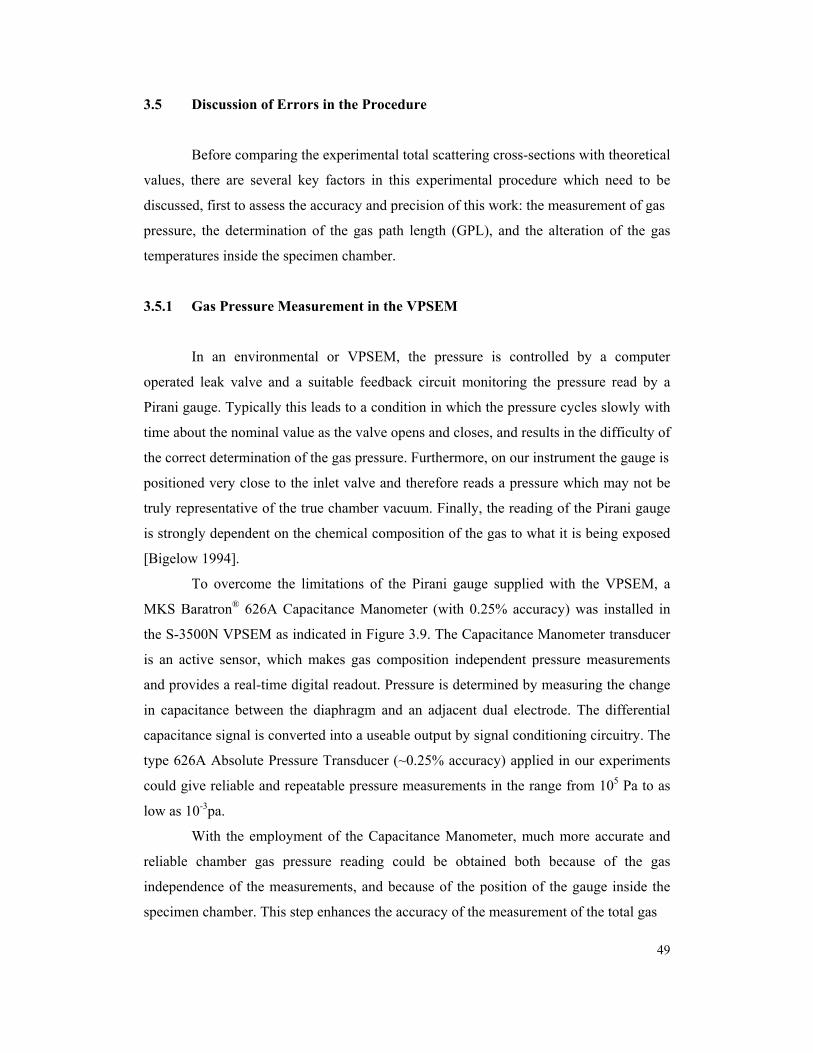
To overcome the limitations of the Pirani gauge supplied with the VPSEM, a

MKS Baratron® 626A Capacitance Manometer (with 0.25% accuracy) was installed in

the S-3500N VPSEM as indicated in Figure 3.9. The Capacitance Manometer transducer

is an active sensor, which makes gas composition independent pressure measurements

and provides a real-time digital readout. Pressure is determined by measuring the change

in capacitance between the diaphragm and an adjacent dual electrode. The differential

capacitance signal is converted into a useable output by signal conditioning circuitry. The

type 626A Absolute Pressure Transducer (~0.25% accuracy) applied in our experiments

could give reliable and repeatable pressure measurements in the range from 105 Pa to as

low as 10-3pa.

With the employment of the Capacitance Manometer, much more accurate and

reliable chamber gas pressure reading could be obtained both because of the gas

independence of the measurements, and because of the position of the gauge inside the

specimen chamber. This step enhances the accuracy of the measurement of the total gas

49

Capacitance manometer

Figure 3.9 MKS Baratron® 626A capacitance manometer.

50

scattering cross-section. For a given pressure setting the observed time varying

fluctuation in pressure was typically a few percent.

The pressures of the gases of interest were measured by the manometer

capacitance, and all the pressure readings along with the nominal pressure readings from

the Pirani gauge were plotted in Figure 3.10. The deviations of the pressure readings from

these two gauges are obvious, even for laboratory air.

3.5.2 Confirmation of the Gas Path Length

The calculation of the scattering cross-section also depends on the value of the

Gas Path Length (GPL), which is the distance through which the incident beam travels

between the Pressure Limiting Aperture (PLA) and the specimen surface. The nominal

working distance was considered to be the GPL in the cross-section calculation, but the

actual GPL may be longer due to the fact that some gases may enter the upper column

through the PLA.

A test was therefore conducted to confirm the correct effective value of the GPL.

Two successive experimental runs were carried out under identical conditions but with

the sample shied by 1mm to change the GPL by a known amount (Figure 3.11). An

application of Eq.3.1 and 3.2 give a value for D which is consistent with the nominal

value of D = 12 mm. This indicates that the high pressure region through which the beam

passes is confined to the area beneath the pressure limiting aperture which is positioned at

the bottom surface of the lens, and that there is no significant penetration of the chamber

gas above the PLA for the pressures used in these experiments [Gauvin et al. 2002]. It is

therefore correct to equate the working distance and GPL in this case.

3.5.3 Confirmation of the Temperature Variation

The computed value of σT depends directly on the assumed temperature of the

gas. The actual temperature of the gas inside the chamber would be expected to be

significantly lower than its temperature outside the chamber because the expansion of the

gas into the low vacuum of the SEM chamber causes cooling.

A sensitive thermocouple was installed on the VPSEM to test the temperature

variation and positioned close to the inlet gas jet in the specimen chamber. During the

51

0

50

100

150

200

250

300

0 50 100 150 200 250 300

Indicated Pressure Reading (Pa)

Man

omet

er P

ress

ure

Rea

ding

s (Pa

)

AirHeArgonCH4

Figure 3.10 Pressure readings by capacitance manometer and Pirani gauge.

52

7

8

9

10

11

12

0 30 60 90 120 150 180 210 240 270 Pressure (Pa)

ln(c

ount

s)

Original position

Lower position

Figure 3.11 Comparison of the collected X-ray signals at two GPLs.

53

pumping down process, the temperature did initially drop from 26.3°C to 23.0°C

within several seconds, but as the gas pressure stabilized at the desired level, the gas

temperature

recovered almost to the starting value, with a very small deviation of around 0.1°C,

suggesting that the gas rapidly achieves thermal equilibrium by contact with the chamber

walls. Therefore, based on our measurement of the temperature variation, on average, the

gas temperature is considered as constant and equal to normal room temperature during

the whole experimental process.

3.5.4 Possible Noise Signals from the Background

The X-ray intensity is expected to decrease with the increasing of the gas

pressure, as more and more electrons are scattered outside the beam, resulting in a

decrease in the collected emission signals from the Al wire. However, from the raw data

we can see that the tendency of the signal variation is not exactly as we expected, there

are some spikes in the initial part of the curve instead of smooth decreasing curve. One of

the possible reasons is probably rising from the background noises.

Based on this observation, the background signals were recorded while the

selected X-ray signals were collecting at each pressure level. Since the characteristic

energy of Alkα is 1.5keV, so the energy range of the recorded background of the Alkα

peak in the spectrum was selected as 2keV to 6keV. The experiments processed under

15keV and 20keV are plotted in Figure 3.12.

From the recorded background signals we can see that they are exhibiting the

same variation as the collected signals during most of the processing time, decreasing

with the increase of the gas pressure and some fluctuations appear at lower gas pressures

range. So, obviously the background signals are not the reason for the fluctuations in the

Al kα signal collection. However the constant background signals during the

measurement, which may be related with the variation of the emission current of the

electron probe, could result some measuring errors in the whole experimental procedure.

Since it is the natural logarithm of the X-ray intensity that we are concerning

about right now, the deviations at the lower pressure range are presently considered as

acceptable factor for our experiments as long as they won’t affect the linear relationship

54

0

1000

2000

3000

4000

5000

6000

7000

8000

0 50 100 150 200 250 300

Pressure (Pa)

Cou

nnts

15keV

20keV

Figure 3.12 Background signals under 15keV and 20keV.

55

between the loge(Intensity) and gas pressure. The background signal factor is therefore

ignored presently and it will be considered in our further researches.

3.6 Experimental Results Discussion

So far the experimental data has been collected for four gases: He, Air, Methane,

and Argon. Excellent agreement is found with values computed from the theory of Jost

and Kessler [Danilatos 1988] over the energy range of 10-30keV used in the experiments.

The experimentally obtained total scattering cross-section for Helium is plotted and

compared with theoretical values in Figure 3.13, and the cross-sections from experiment

and theory agree very well. There is some deviation at lower beam energies, which may

due to the omission from the theoretical model of some possible inelastic contributions to

the cross-section.

In the pressure range used for this work, many gases are believed to be molecular

rather than atomic in nature. The so-called “van der Waals bounded complex” was

discovered in 1965 are atomic clusters that can be simply created by the expansion of a

jet of gas into vacuum. The cooling associated with the gas’s adiabatic expansion causes

the gas to supersaturate and the atoms nucleate into clusters. These macromolecules

systems have caused much attention because they appear to bridge the gap between a

molecular and a bulk solid state form of matter.

How large does an assemblage of single atoms have to become before it begins to

take on the properties of a bulk solid? The answer depends on the characteristics of the

studied material (e.g., Ar clusters: > 2000 atoms, Li clusters: > 130 atoms and V clusters:

> 30). Atoms and Molecules in clusters behave in a different manner to those contained

in liquid or solid substances. In spite of its size, behaviors of cluster do not simply evolve

continuously from those of an atomic to macroscopic scale [Ditmire 1997]. So, the total

scattering cross-section for a molecule may be not just the sum of the atomic cross-

section. Additional interactions with the incident electron beam are very possible due to

binding of atoms in molecules, considering the outer region is primarily responsible for

scattering at the smallest angles [Danilatos 1988]. Both the theoretical molecular cross-

section and atomic cross-section for Nitrogen were plotted in Figure 3.14 and it clearly

verifies that the molecular cross-section of N is larger than just simply twice the atomic

cross-section value of N. The differences increase at the lower beam energy range.

56

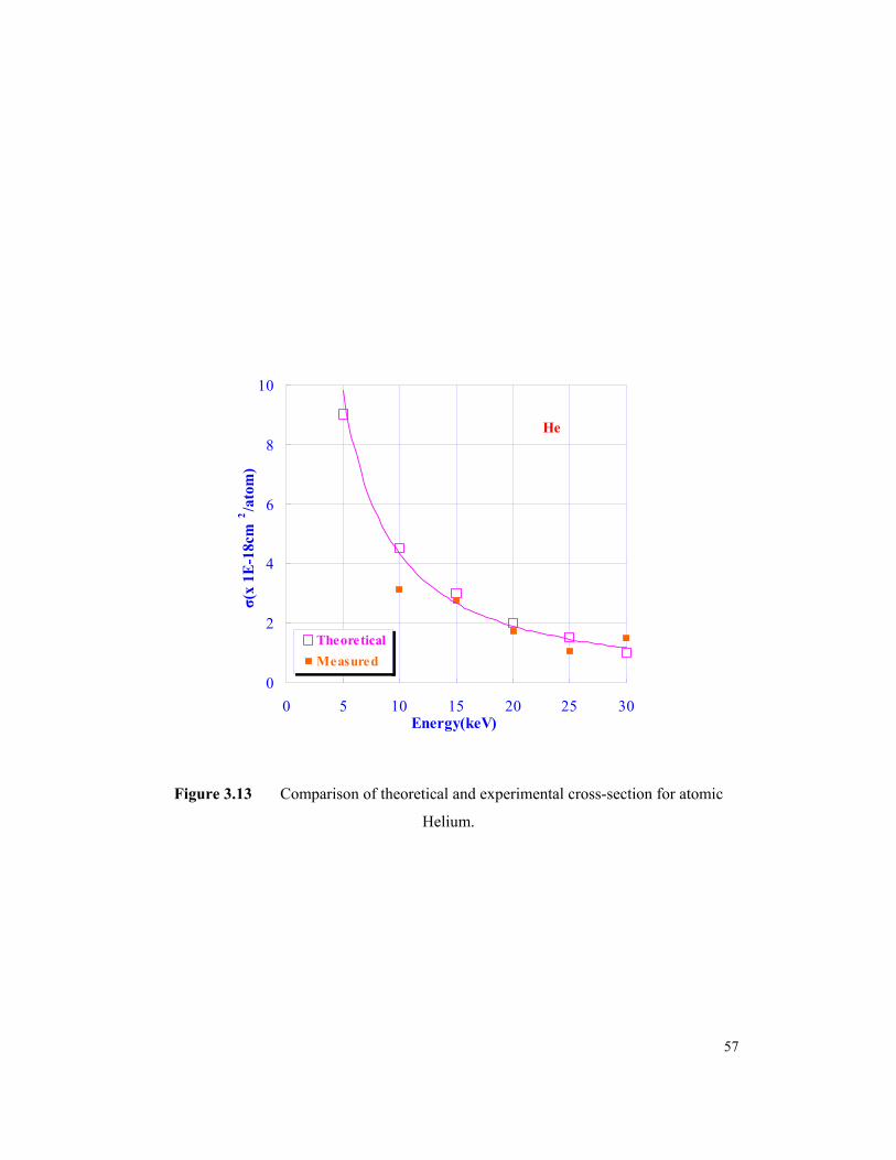
0

2

4

6

8

10

0 5 10 15 20 25 30Energy(keV)

σ(x

1E-1

8cm

2 /ato

m)

Theoretical

He

Measured

Figure 3.13 Comparison of theoretical and experimental cross-section for atomic

Helium.

57

0

2

4

6

8

10

4 6 8 10 12 14 16 18 20

Energy(keV)

σ (x

1E-1

7cm

2 /ato

m)

Molecular N

N2

Atomic N

Figure 3.14 Theoretical cross-section for atomic and molecular Nitrogen.

58

Since the most commonly used chamber gas is ‘laboratory’ air, the collected

experimental data of total scattering cross-section for air is compared with theoretical

total cross-sections of atomic N, molecular N2, molecular O2 (the curve for O2 lies just

below that of N2 and is not shown for clarity) and water vapor in Figure 3.15. As

demonstrated by the curves, the measured total scattering cross-section for air tracks

closely with that for molecular rather than atomic Nitrogen. It is higher than the value for

water vapor (at Room Temperature and Pressure) as expected since the partial pressure of

the water vapor is below the saturation value.

3.7 Summary

The experimental total scattering cross-section data obtained in these

experiments is of great interest. It shows the excellent agreement between experimental

values and theoretical estimates of the total gas scattering cross-section. The new method

of the measurement of the gas scattering cross-section has been validated by this data and

the predicted linear relationship between loge(Ip/I0) and gas pressure has also been

confirmed.

On the basis of the available evidence, gases tend to be molecular rather than

atomic in nature in the pressure range used in the performed experiments. During the

experimental procedure, the temperature variation could be ignored in our calculation in

average and it is also reliable to equate the working distance of the VPSEM to the gas

path length (GPL) in calculations of the scattering cross-section.

In our future work the total cross-sections of more complex gases, such as XeF2,

W(CO)6 etc. metallic gases selectively used for etching and depositing will be measured

and a more precisely controlled method of gas induction, for example, a localized small

gas jet with needle valve to position gases to just the area around specimen, will be tested

and used in further experiments. In next of this work, the experimentally collected gas

scattering cross-section data will be inserted into Monte Carlo simulation program to

predict the spatial distribution of the electron beam scattering under given beam energy.

59

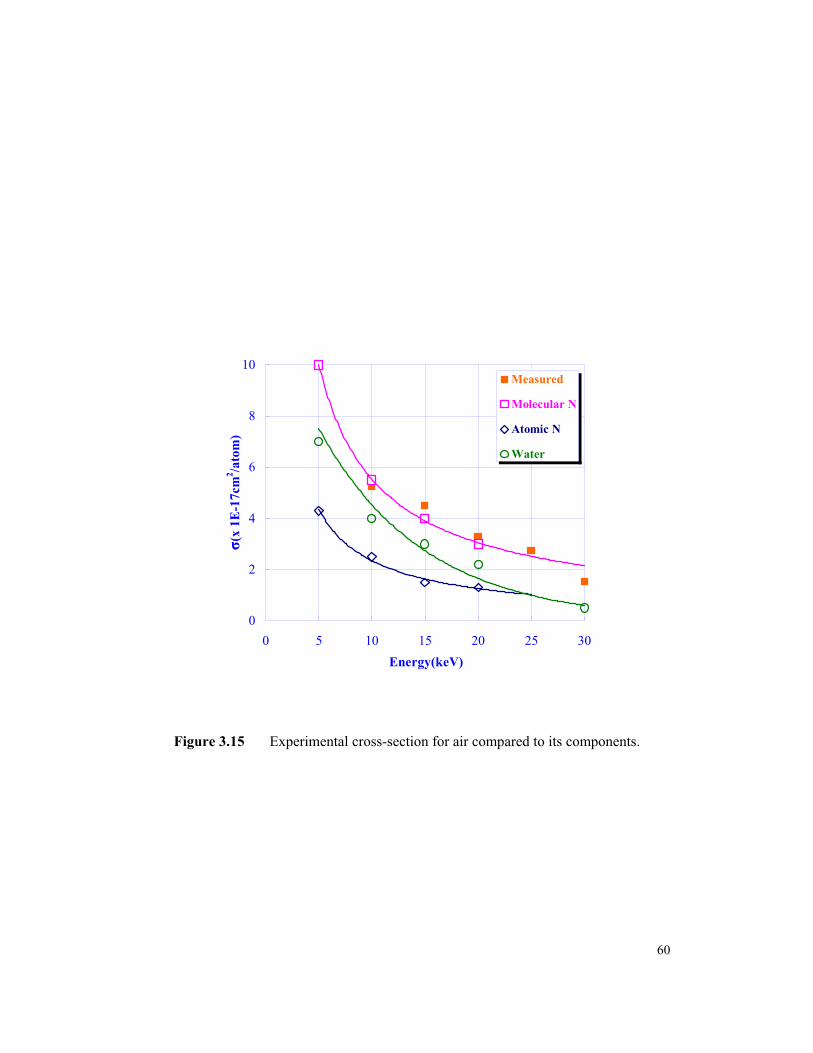
0

2

4

6

8

10

0 5 10 15 20 25 30Energy(keV)

σ(x

1E-1

7cm

2 /ato

m)

Molecular N

Atomic N

Measured

Water

Figure 3.15 Experimental cross-section for air compared to its components.

60

CHAPTER IV

MONTE CARLO SIMULATION OF THE ELECTRON BEAM SCATTERING

4.1 Introduction of Monte Carlo simulation

4.1.1 Background Introduction

Monte Carlo simulation as it is often called should more correctly be titled Monte

Carlo sampling since it uses random numbers to sample either experimental or theoretical

data. The first published example of the use of random numbers to solve problem is that

of Buffon, who-in his 1777 volume Essai d’ Arithmetique Morale-describe an experiment

in which needles with equal length were thrown randomly over a sheet marked with

parallel lines. Amazingly, by counting the number of intersections between lines and

needles, Buffon was able to derive a value for π. Subsequently many other

mathematicians and statisticians followed Buffon’s lead and started to use random

numbers as a way of testing theories and results. For example, in the early twentieth

century, radioactive decay or the transmissions of cosmic rays through barriers all have

been investigated by random numbers [Joy 1995].

Monte Carlo sampling techniques was known by its extensively application during

the Manhattan project by Von Neumann and Stan Ulam, who refined this investigation as

" Russian roulette" and "splitting" methods at that time. They made use of both random-

number sampling and game-playing situations involving random numbers as a way of

studying physical processes as diverse as neutron diffusion and the probability of a

missile striking a flying aircraft. But Enrico Fermi was actually the first scientist who had

independently developed the Monte Carlo method in the early 1930’s when he was

studying the moderation of neutrons in Rome. Then during the hiatus in the ENIAC (first

electronic computer) operation in 1947, he built an instrument called the FERMIAC to

develop neutron genealogies in two dimensions by generating the site of the “ next

collision”. Each generation was based on a choice of parameters that characterized the

particular material being traversed. About 1948 Fermi, Metropolis, and Ulam obtained

Monte Carlo estimates for the eigenvalues of Schrodinger equation [Metropolis 1987].

Nowadays the Monte Carlo method has a wide range of applications, from the simulation

61

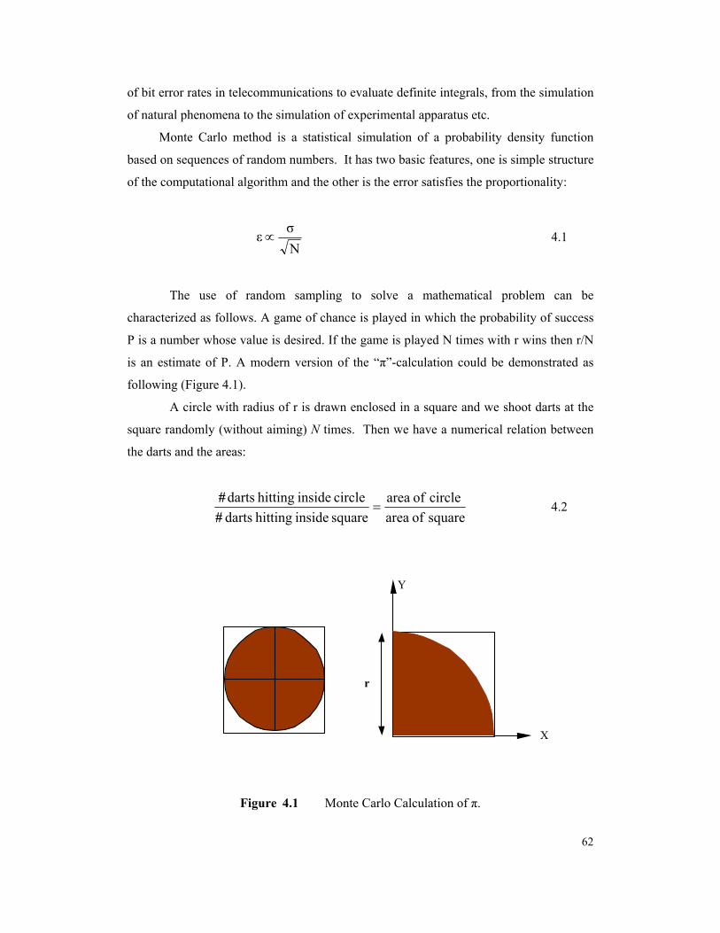
of bit error rates in telecommunications to evaluate definite integrals, from the simulation

of natural phenomena to the simulation of experimental apparatus etc.

Monte Carlo method is a statistical simulation of a probability density function

based on sequences of random numbers. It has two basic features, one is simple structure

of the computational algorithm and the other is the error satisfies the proportionality:

Nσε ∝ 4.1

The use of random sampling to solve a mathematical problem can be

characterized as follows. A game of chance is played in which the probability of success

P is a number whose value is desired. If the game is played N times with r wins then r/N

is an estimate of P. A modern version of the “π”-calculation could be demonstrated as

following (Figure 4.1).

A circle with radius of r is drawn enclosed in a square and we shoot darts at the

square randomly (without aiming) N times. Then we have a numerical relation between

the darts and the areas:

square inside hitting dartscircle insidehitting darts

# #

squareof area circle of area

= 4.2

Y

X

r

Figure 4.1 Monte Carlo Calculation of π.

62

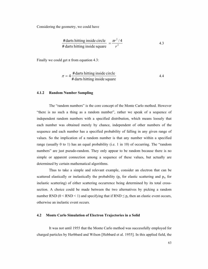
Considering the geometry, we could have

square inside hitting dartscircle insidehitting darts

# #

2

2 4/r

rπ= 4.3

Finally we could get π from equation 4.3:

square inside hitting dartscircle insidehitting darts4

# #

=π 4.4

4.1.2 Random Number Sampling

The “random numbers” is the core concept of the Monte Carlo method. However

“there is no such a thing as a random number”, rather we speak of a sequence of

independent random numbers with a specified distribution, which means loosely that

each number was obtained merely by chance, independent of other numbers of the

sequence and each number has a specified probability of falling in any given range of

values. So the implication of a random number is that any number within a specified

range (usually 0 to 1) has an equal probability (i.e. 1 in 10) of occurring. The “random

numbers” are just pseudo-random. They only appear to be random because there is no

simple or apparent connection among a sequence of these values, but actually are

determined by certain mathematical algorithms.

Thus to take a simple and relevant example, consider an electron that can be

scattered elastically or inelastically the probability (pe for elastic scattering and pie for

inelastic scattering) of either scattering occurrence being determined by its total cross-

section. A choice could be made between the two alternatives by picking a random

number RND (0 < RND < 1) and specifying that if RND ≤ pe then an elastic event occurs,

otherwise an inelastic event occurs.

4.2 Monte Carlo Simulation of Electron Trajectories in a Solid

It was not until 1955 that the Monte Carlo method was successfully employed for

charged particles by Herbbard and Wilson [Hebbard et al. 1955]. In this applied field, the

63

Monte Carlo technique using random numbers as a means of predicting the magnitude of

various events and as a way for selecting between possible scattering options [Joy 1995].

Before ultimately losing its energy or escaping from the specimen, each incident electron

may undergo hundreds or thousands of separate scattering events, distributed between

elastic and a variety of inelastic processes. It is necessary to be able to describe in detail

the processes, which produced that data in the first place, but this is not a simple task

because the interaction between the electron beam with a solid is highly complex. The

Monte Carlo method was therefore developed for the quantitatively study of the electron

microscopy technique to correctly interpret images or spectra.

4.2.1 Basic Principle

The Monte Carlo technique, as applied in the electron microscopy field, attempts

to describe the trajectory which takes the electron through the solid. Although no

individual trajectory produced by the simulation will represent a real trajectory, if the

physics of the processes encountered (Figure 4.2) by the electron are properly modeled

then predictions based on a large number of trajectories will accurately describe effects

which can be experimentally observed. In order to make these calculation possible, two

basic pieces of information, the scattering angle, through which the electron is scattered

and the average step length between two successive scattering events given particular

incident energy are required [Joy, 1995].

The basic principle of this application [Goldstein et al., 1992] is that the step

length of the basic repetitive step in such a calculation is usually set as some fraction of

the Mean Free Path (i.e. the average distance traversed by a molecule between collisions,

as introduced before, it is a key parameter related with the electron scattering study and

the Mean Free Path (MFP) of an electron in a solid is strongly dependent on its kinetic

energy) for elastic scattering ("single scattering Monte Carlo") or a multiple scattering

("multiple scattering Monte Carlo"). From the Mean Free Path and the rate of energy loss

due to inelastic scattering as calculated with the Bethe [Bethe et al. 1930] or Joy-Luo [Joy

et al. 1989] expressions, the loss of energy can be calculated along the path of the

electron. After the electron travels a distance equal to the Mean Free Path, the next

scattering site is reached, and a new scattering angle is chosen for the next step based

upon the new value of the energy. Since the elastic scattering angle can take on any value

64

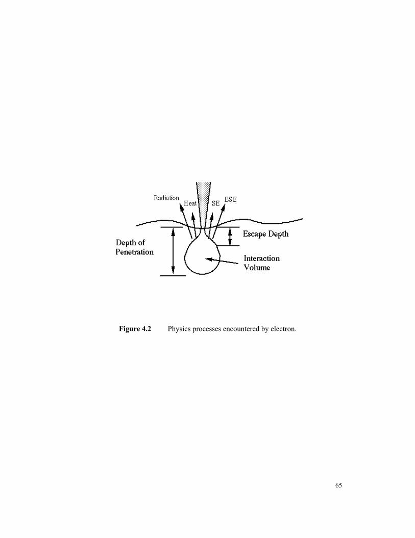
Figure 4.2 Physics processes encountered by electron.

65

over a wide range from 0 to 180 degrees, random numbers are used with an appropriate

weighting factor to produce the appropriate statistical distribution of scattering. Because

of the extensive use of random numbers in the simulation, the name "Monte Carlo" is

applied to this technique.

4.2.2 Assumptions for Original Model

There are two major approximations based on which the original model was

established.

(1) Only elastic scattering events described by the Rutherford cross-section are

significant in determining the path taken by any given electron as it moves through the

solid. As described in chapter I, there are essentially two kinds of the scattering, elastic

scattering and inelastic scattering. The elastic scattering happens when the electrons

repulsed by the orbital electrons of the nucleus while undergo the Columbic attraction

from the positively charged nucleus of the target atom. During elastic scattering, a large

range (5°~180°) of scattering angles could be covered [Edgerton 1996], though only less

than 1eV energy loss from the incident electron to the target atom. On the other hand, the

majority of the inelastic scattering produce angular deflections of typically 0.5° or less,

but with large fraction of the energy loss. Consequently the elastic scattering dominate in

determining the path of the trajectory of the electrons and ignoring the inelastic effects

introduces only negligible error while greatly reducing the number of computations that

may be required.

(2) The energy loss of the incident electrons is assumed to be a continuous

process along their path at a rate determined by Bethe [Bethe et al. 1930] relationship,

instead of as the result of discrete inelastic scattering events. In reality the continuous

energy loss, such as Bremsstrahlung emission, and the discrete energy loss like Plasmons

and Characteristic X-rays excitation created simultaneously, so Bethe average these

energy loss processes and created Bethe relationship for the single scattering model

[Bethe et al. 1930].

4.2.3 Statistics of the Original Model

66

Examination of the individual trajectories in Figure 4.3 (a output of the simulation)

reveals that each trajectory varies greatly from any of the others because of the random

selection from the range of scattering parameters.

Therefore the principal weakness of the Monte Carlo calculation is the need to

calculate many trajectories in order to obtain statistical significance [Holt 1989]. In order

to calculate results, which are representative of the overall interaction a statistically

significant number of trajectories must be calculated. The precision of a Monte Carlo

calculation depends on the number of events calculated, with the standard deviation of

the calculation given by the expression:

SD = iN 4.4

Where Ni is the number of trajectories, which contribute to an event of type i. The

relative standard deviations then given by

RSD = i

i

NN

= iN

1 4.5

Thus in a calculation of a back scattering coefficient, the precision of the calculation is

not determined by the total number of electrons calculated, N but by the number of

electron which back scatter;

Ni =ηN 4.6

In the same simulation, the calculation of characteristic X-ray production would be

obtained with greater precision, since all of the incident electrons contribute to the

generation of X-rays.

Why is Monte Carlo technique used so extensively? Most of the time, for each

possible values and the probability distribution of the interested variable is always

unknown in the case of reality. Although the statistical estimation could provide a value

that is as close as possible to the actual unknown value, based on some definition of

goodness or quality, the Monte Carlo simulation is always chosen since it can provide a

67

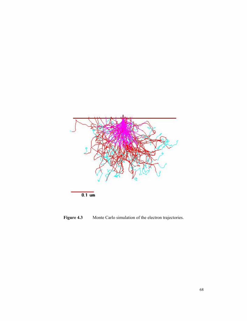
Figure 4.3 Monte Carlo simulation of the electron trajectories.

68

model uncertainty before and after a transfer function.

4.3 New Monte Carlo Simulation for Gas

4.3.1 Why Use This Method?

In the gaseous environmental SEM the incident electron beam is scattered when

it passes through the low pressure gas atmosphere and results in a broadening of the

electron probe, and a reduction in the current available for imaging and analysis.

Moreover, the production of the secondary ions from the scattering can also impact the

specimen and modify the production of secondary and backscattered electrons.

As we discussed before, to optimize and fully exploit the capabilities of gaseous

environmental SEMs and the interaction between the electron beam and gas molecules, it

is desirable to be able to accurately predict these effects of various micro-particles exists

in the gaseous environment. An accurate model of the primary electron beam scattered in

the gaseous environment would enable researchers to predict the magnitude of the

scattered electron “skirt”. Ideally the model would predict the optimum conditions to

utilize efficiently the interaction between electrons and gas molecules and reduce the side

effects on the analytical spatial resolution caused by scattering for a given gaseous

system. Alternatively, it also would be used to develop a correction to the analytical data

that reduces the effect of the scattered electron generated x-rays from the spectra. By

using the Monte Carlo method and our measured cross-sections we can predict scattering

profiles and compare these with our measured data.

Simple functional relations about these most concerned parameters could always

be derived based on certain amount of assumptions. Based on this definition of the Mean

Free Path length, at a gas pressure of 100 Pa, the Mean Free Path for 20 keV electrons is

of the order of 1 cm. Therefore for a typical working distance of approximate 10mm, the

average electron is only scattered once. Under this condition, one of the first

approximation to the modification of the incident probe was established by estimating a

mean scattering angle, Φ and assuming that this event occurs at the mid-point of the

trajectory.

23

21

21 19.364 L

TP

EZr

= 4.7

69

This equation has been adapted from the original version due to Reimer [1985] to include

pressure and to be in SI units (E in eV). Goldstein [Goldstein et al. 1977] had previously

derived the same formula except with a numerical factor 5.95 times larger. Smith and

Schumacher [1974] have also produced a formula for the half width broadening given by

( )( ) 2

321

3/10

221 192ln12.793 L

ZTpZZ

EEr

+

+=

ββ

4.8

where

21

2

0

1

11

+

−=

EE

β 4.9

These relations have been demonstrated by several authors and represent a

relativistic correction to give a useful estimate of the beam broadening [Farley et al.

1990].

However to quantitatively predict the behavior of the primary electron beam to

adequately describe the beam profile as it reaches the specimen surface, a Monte Carlo

simulation of should be a optimal choice. "GASSEM", a Monte Carlo simulation model

was therefore developed.

4.3.2 How We Did It?

In our study, although the electron is scattered due to its collision with the gas

molecule instead of solid molecule, the basic single scattering Monte Carlo model

mentioned before could still be used because the gas is treated as a dilute solid here.

4.3.2.1 Include Inelastic and Elastic Scattering

In our new model, one major difference from the original model is that both the

elastic and inelastic scattering events are included. Inelastic scattering has no effect on

70

the formation of the beam skirt because the scattering angles are too small by comparison

with the elastic deflections. But inelastic events are crucial in determing the broadening

of the focused probe.

The inelastic scattering was neglected and considered insignificant in

determining the electron trajectory, because the deflection angle of the inelastic scattering

is small (<1°). Due to the increasing requirement of the micro, even sub-micro scale

products in the market, resolution of the technique in related development and research

area is also becoming smaller and smaller. So the small angle scattering events are

becoming causing more and more attention

In the small angle scattering area, the inelastic scattering events are in fact the

majority of the scattering as indicated by Figure 4.4. It is also believed that it is the

inelastic events, which determine the form of the beam profile close to (i.e. within a few

micrometers of) the axis, and the relative higher angle elastic events determine the width

and magnitude of the large scattered region which surrounds the beam [Joy 1995].

Therefore we can not ignore the inelastic scattering any more and both elastic and

inelastic scattering will be included in the new model.

Since the scattering angle is so small for the inelastic scattering, it is relative difficult to

obtain a set of inelastic scattering cross-sections by experiments based on our

experiences. Moreover, most of the theoretical inelastic cross-section values derived

based upon several approximations, which may not reliable for us to use in this model.

Considering the possibility of the elastic scattering event is less than that of the inelastic

scattering events, in the simulation, the ratio of inelastic scattering /elastic is selected by

random numbers based on the assumption that the cross-section for inelastic scattering is

some selected factor –typically 10 times of the elastic scattering cross-sections.

4.3.2.2 Single Scattering Model

It is also believed that in the regime of the interested collision of the incident

electron beam and the surrounding gas molecules, the majority of the electrons still

undergoing about one scattering event. So a single scattering model was established

based on the original model by Joy [1995,1996] with some revision.

71

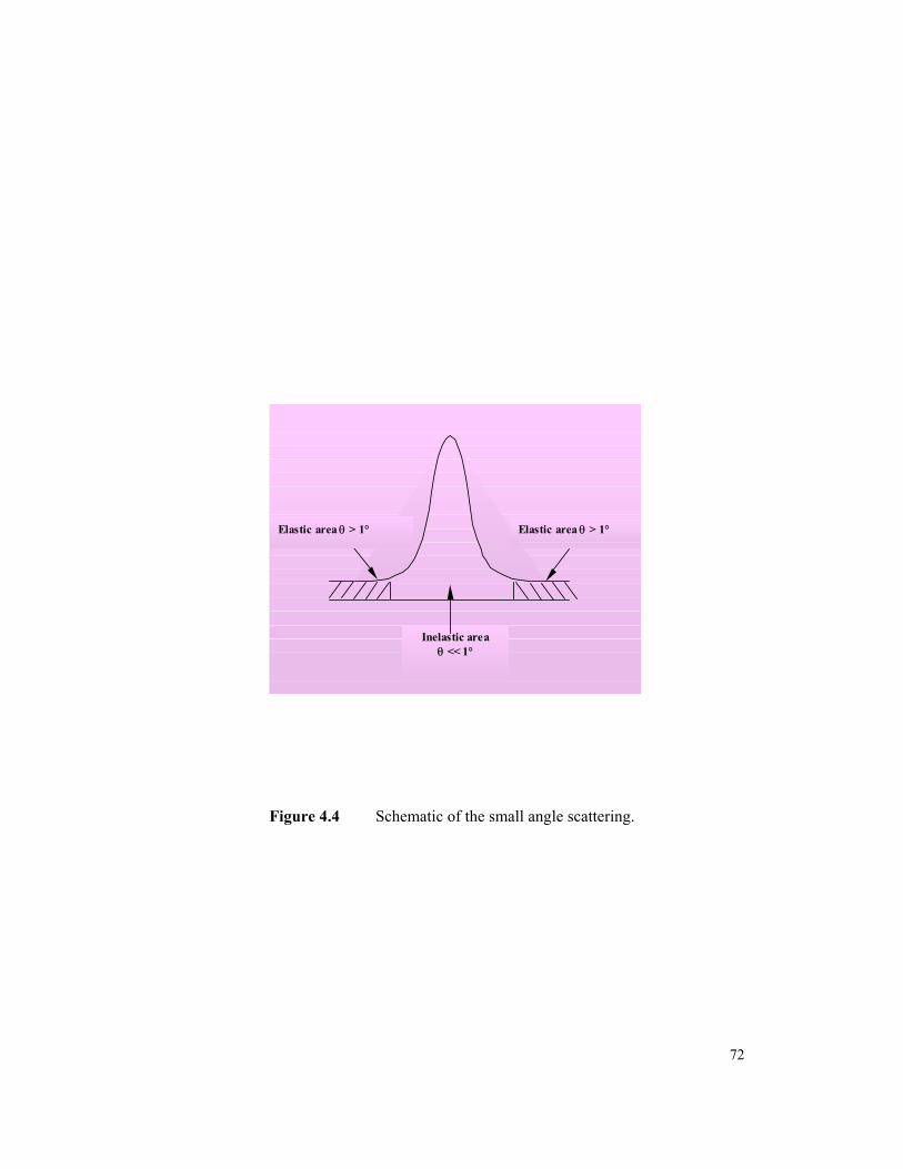
Elastic area θ > 1°

Inelastic area θ << 1°

Elastic area θ > 1°

Figure 4.4 Schematic of the small angle scattering.

72

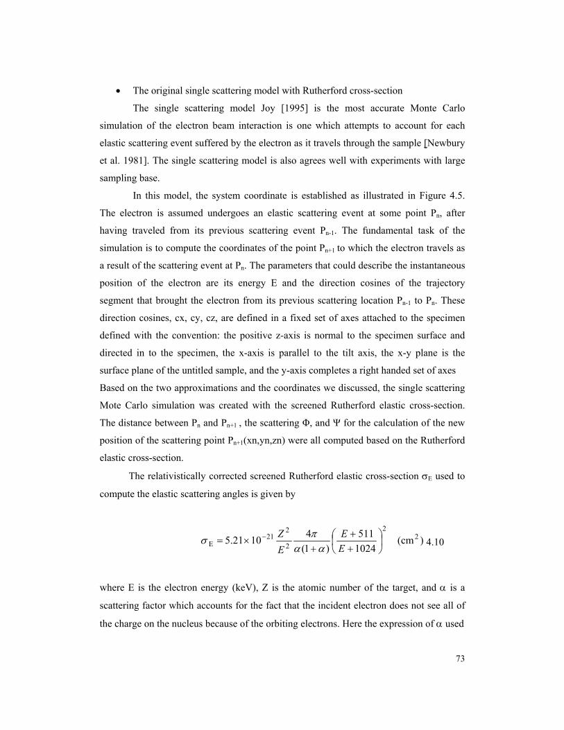
• The original single scattering model with Rutherford cross-section

The single scattering model Joy [1995] is the most accurate Monte Carlo

simulation of the electron beam interaction is one which attempts to account for each

elastic scattering event suffered by the electron as it travels through the sample [Newbury

et al. 1981]. The single scattering model is also agrees well with experiments with large

sampling base.

In this model, the system coordinate is established as illustrated in Figure 4.5.

The electron is assumed undergoes an elastic scattering event at some point Pn, after

having traveled from its previous scattering event Pn-1. The fundamental task of the

simulation is to compute the coordinates of the point Pn+1 to which the electron travels as

a result of the scattering event at Pn. The parameters that could describe the instantaneous

position of the electron are its energy E and the direction cosines of the trajectory

segment that brought the electron from its previous scattering location Pn-1 to Pn. These

direction cosines, cx, cy, cz, are defined in a fixed set of axes attached to the specimen

defined with the convention: the positive z-axis is normal to the specimen surface and

directed in to the specimen, the x-axis is parallel to the tilt axis, the x-y plane is the

surface plane of the untitled sample, and the y-axis completes a right handed set of axes

Based on the two approximations and the coordinates we discussed, the single scattering

Mote Carlo simulation was created with the screened Rutherford elastic cross-section.

The distance between Pn and Pn+1 , the scattering Φ, and Ψ for the calculation of the new

position of the scattering point Pn+1(xn,yn,zn) were all computed based on the Rutherford

elastic cross-section.

The relativistically corrected screened Rutherford elastic cross-section σE used to

compute the elastic scattering angles is given by

)cm( 1024511

)1(41021.5 2

2

2

221

E

++

+×= −

EE

EZ

ααπσ 4.10

where E is the electron energy (keV), Z is the atomic number of the target, and α is a

scattering factor which accounts for the fact that the incident electron does not see all of

the charge on the nucleus because of the orbiting electrons. Here the expression of α used

73

cc

cb

X

Y

Z

Step ψ

φ

Pn+1, En+1

Pn, En Z

cz cy

cx

P n - 1 E n - 1 Fixed Set of Axes

Y

X

Figure 4.5 Coordinate system for Monte Carlo simulation

74

is [Bishop 1976]

2

67.03104.3

EZ−×=α 4.11

With the elastic cross-section, the Mean Free Path λ could be computed by

(cm) EaN

Aρσ

λ = 4.12

where Na is Avagadro’s number, is the density (gm/cm3) and A is the atomic

weight(gm/mole). The value of Mean Free Path depends both on the beam energy and on

the characteristics of the specimen, but is typically of the order of a few hundred

angstroms at 100keV. The actual distance that an electron travel between successive

scattering will vary in a random fashion, that is why we introduce this variability in the

Monte Carlo simulation by saying that the step length between Pn(x,y,z) and

Pn+1(xn,yn,zn) is given by the relation

Step = -λ ln (RND) (cm) 4.13

Where RND is an uniformly distributed random number between (0, 1) automatically

selected by computer.

In the scattering event at Pn(x,y,z) which marks the start of this step, the electron

is deflected through angle Φ (scattering angle) relative to its previous direction. This

deviation is determined by the angular differential form of the Rutherford cross-section,

Ω=′

dd Eσσ and in our program is derived by solving

d RND0

Ω′

= ∫φ

σσ

E 4.14

75

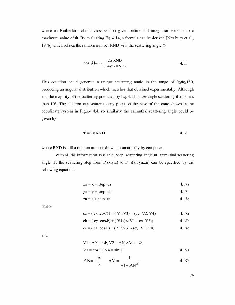
where σE Rutherford elastic cross-section given before and integration extends to a

maximum value of Φ. By evaluating Eq. 4.14, a formula can be derived [Newbury et al.,

1976] which relates the random number RND with the scattering angle Φ,

( ) RND)- (1

RND 2 -1 cosααφ

+= 4.15

This equation could generate a unique scattering angle in the range of 0≤Φ≤180,

producing an angular distribution which matches that obtained experimentally. Although

and the majority of the scattering predicted by Eq. 4.15 is low angle scattering-that is less

than 10°. The electron can scatter to any point on the base of the cone shown in the

coordinate system in Figure 4.4, so similarly the azimuthal scattering angle could be

given by

Ψ = 2π RND 4.16

where RND is still a random number drawn automatically by computer.

With all the information available, Step, scattering angle Φ, azimuthal scattering

angle Ψ, the scattering step from Pn(x,y,z) to Pn+1(xn,yn,zn) can be specified by the

following equations:

xn = x + step. ca 4.17a

yn = y + step. cb 4.17b

zn = z + step. cc 4.17c

where

ca = ( cx .cosΦ) + ( V1.V3) + (cy. V2. V4) 4.18a

cb = ( cy .cosΦ) + ( V4.(cz.V1 – cx. V2)) 4.18b

cc = ( cz .cosΦ) + ( V2.V3) - (cy. V1. V4) 4.18c

and

V1 =AN.sinΦ, V2 = AN.AM.sinΦ,

V3 = cos Ψ, V4 = sin Ψ 4.19a

z

- ANccx

= 2AN 1

1 +

=AM 4.19b

76

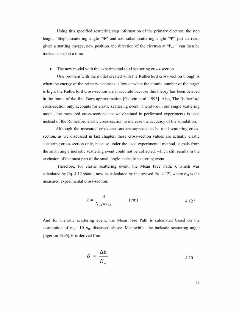
Using this specified scattering step information of the primary electron, the step

length “Step”, scattering angle “Φ” and azimuthal scattering angle “Ψ” just derived,

given a starting energy, new position and direction of the electron at “Pn+1” can then be

tracked a step at a time.

• The new model with the experimental total scattering cross-section

One problem with the model created with the Rutherford cross-section though is

when the energy of the primary electrons is low or when the atomic number of the target

is high, the Rutherford cross-section are inaccurate because this theory has been derived

in the frame of the first Born approximation [Gauvin et al. 1993]. Also, The Rutherford

cross-section only accounts for elastic scattering event. Therefore in our single scattering

model, the measured cross-section data we obtained in performed experiments is used

instead of the Rutherford elastic cross-section to increase the accuracy of the simulation.

Although the measured cross-sections are supposed to be total scattering cross-

section, as we discussed in last chapter, these cross-section values are actually elastic

scattering cross-section only, because under the used experimental method, signals from

the small angle inelastic scattering event could not be collected, which still results in the

exclusion of the most part of the small angle inelastic scattering event.

Therefore, for elastic scattering event, the Mean Free Path, λ which was

calculated by Eq. 4.12 should now be calculated by the revised Eq. 4.12′, where σM is the

measured experimental cross-section:

(cm) MaN

Aρσ

λ = 4.12 ′

And for inelastic scattering event, the Mean Free Path is calculated based on the

assumption of σIE~ 10 σIE discussed above. Meanwhile, the inelastic scattering angle

[Egerton 1996], θ is derived from

oEE∆

=θ 4.20

77

where ∆E is the energy loss in inelastic event. For the rest of the coordinate calculation,

all the equations listed in the original model are employed.

4.3.2.3 Energy Loss of the Incident Electrons

So far we obtained the new position Pn+1 under possible scattering event, either

inelastic or elastic scattering for one step track, and whether the electron goes to next step

will depend on the how much energy the electron still left.

As the electron travel through the solid its energy loses and since the scattering

event is energy dependent, the instantaneous energy at any time need to be calculated.

The energy loss, denoted by dSdE , could be given by the Bethe [1930] relation as:

−=

JE

AEZ

dS166.1 log78500dE ρ

(keV/cm) 4.21

where J is the mean ionization potential which represents the average rate of energy

transfer due to all possible inelastic events (i.e. the excitation of X-rays, Auger electron,

phonons etc.). At high energies, E > 30 keV, it can be found from Berger and Selzer

[1964] expression:

30.19 10

Z58.5 76.9 −

+= ZJ (keV) 4.22

However, at relative low energy, J also falls due to the possible attribution from the

inelastic scattering events. To solve this problem, Joy and Luo [1989] rewrote the energy

loss equation:

+−= 1166.1 log78500dE

JE

AEZ

dSρ

(keV/cm) 4.23

78

As demonstrated, this expression is accurate down to energies of 100eV only or below,

and also avoids the difficulty in Eq. 4.21, that it can not be evaluated for E<J. Under both

elastic and inelastic scattering events, the energy lost along the step, ∆E, from Pn(x,y,z) to

Pn+1(xn,yn,zn) could be calculated using either Eq. 4.21 or 4.23 as:

∆E = step ( dSdE

) 4.24

4.3.2.4 Schematic Sequence of the Operations

To summarize, the sequence of operations needed to simulate the electron path

through the specimen can now be written out schematically in an algorithmic form:

Repeat

Get starting energy E of electron

Get starting coordinates x, y, z for the step

Get direction cosines cx, cy, cz relative to initial axes

Compute Mean Free Path for energy E and given material

Calculate the step length step from Eq. 4.13

Find the scattering angles from Eq. 4.15, 4.16 for elastic event,

Eq. 4.20 for inelastic scattering

Compute final coordinates xn,yn,zn from Eq.( 4.17, 4.18, 4.19)

Compute finish energy E′=E – step(dE/ds)

Reset coordinates x=xn, y=yn, z=zn

Reset direction cosines cx=ca, cy=cb, cz=cc

Reset energy E=E′

Until electron leaves sample or falls below some minimum energy

This sequence of steps is repeated to simulate 30-60,000 electron trajectories as

required by the desired accuracy.

4.3.2.5 I(r) Radial Beam Distribution Plot

79

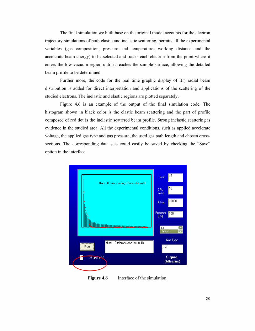
The final simulation we built base on the original model accounts for the electron

trajectory simulations of both elastic and inelastic scattering, permits all the experimental

variables (gas composition, pressure and temperature; working distance and the

accelerate beam energy) to be selected and tracks each electron from the point where it

enters the low vacuum region until it reaches the sample surface, allowing the detailed

beam profile to be determined.

Further more, the code for the real time graphic display of I(r) radial beam

distribution is added for direct interpretation and applications of the scattering of the

studied electrons. The inelastic and elastic regions are plotted separately.

Figure 4.6 is an example of the output of the final simulation code. The

histogram shown in black color is the elastic beam scattering and the part of profile

composed of red dot is the inelastic scattered beam profile. Strong inelastic scattering is

evidence in the studied area. All the experimental conditions, such as applied accelerate

voltage, the applied gas type and gas pressure, the used gas path length and chosen cross-

sections. The corresponding data sets could easily be saved by checking the “Save”

option in the interface.

Figure 4.6 Interface of the simulation.

80

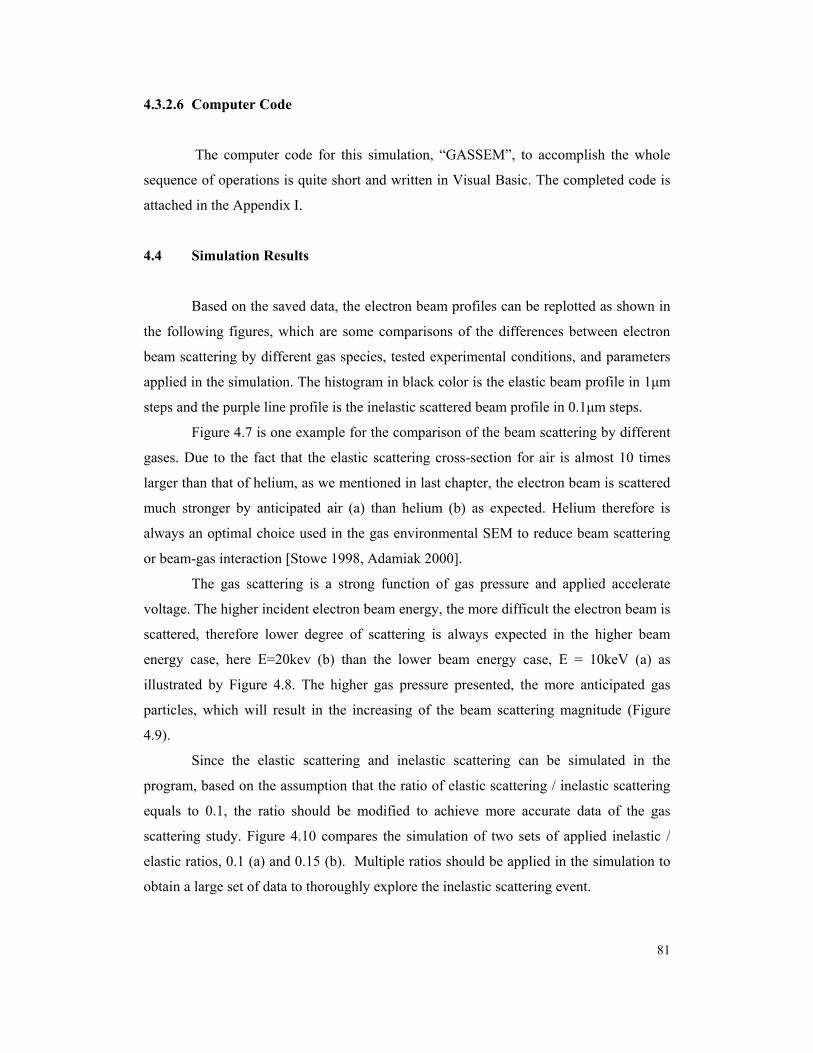
4.3.2.6 Computer Code

The computer code for this simulation, “GASSEM”, to accomplish the whole

sequence of operations is quite short and written in Visual Basic. The completed code is

attached in the Appendix I.

4.4 Simulation Results

Based on the saved data, the electron beam profiles can be replotted as shown in

the following figures, which are some comparisons of the differences between electron

beam scattering by different gas species, tested experimental conditions, and parameters

applied in the simulation. The histogram in black color is the elastic beam profile in 1µm

steps and the purple line profile is the inelastic scattered beam profile in 0.1µm steps.

Figure 4.7 is one example for the comparison of the beam scattering by different

gases. Due to the fact that the elastic scattering cross-section for air is almost 10 times

larger than that of helium, as we mentioned in last chapter, the electron beam is scattered

much stronger by anticipated air (a) than helium (b) as expected. Helium therefore is

always an optimal choice used in the gas environmental SEM to reduce beam scattering

or beam-gas interaction [Stowe 1998, Adamiak 2000].

The gas scattering is a strong function of gas pressure and applied accelerate

voltage. The higher incident electron beam energy, the more difficult the electron beam is

scattered, therefore lower degree of scattering is always expected in the higher beam

energy case, here E=20kev (b) than the lower beam energy case, E = 10keV (a) as

illustrated by Figure 4.8. The higher gas pressure presented, the more anticipated gas

particles, which will result in the increasing of the beam scattering magnitude (Figure

4.9).

Since the elastic scattering and inelastic scattering can be simulated in the

program, based on the assumption that the ratio of elastic scattering / inelastic scattering

equals to 0.1, the ratio should be modified to achieve more accurate data of the gas

scattering study. Figure 4.10 compares the simulation of two sets of applied inelastic /

elastic ratios, 0.1 (a) and 0.15 (b). Multiple ratios should be applied in the simulation to

obtain a large set of data to thoroughly explore the inelastic scattering event.

81

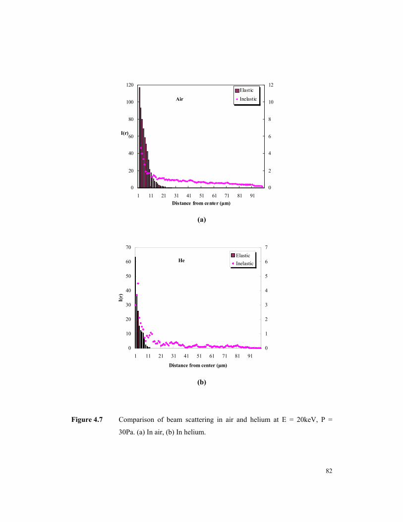
(a)

Air

0

20

40

60

80

100

120

1 11 21 31 41 51 61 71 81 91Distance from center (µm)

I(r)

0

2

4

6

8

10

12Elastic

Inelastic

He

0

10

20

30

40

50

60

70

1 11 21 31 41 51 61 71 81 91

Distance from center (µm)

I(r)

0

1

2

3

4

5

6

7ElasticInelastic

(b)

Figure 4.7 Comparison of beam scattering in air and helium at E = 20keV, P =

30Pa. (a) In air, (b) In helium.

82

(a)

10kV

0 2 4 6 8

10 12 14 16 18 20

1 11 21 31 41 51 61 71 81 91

Distance from center (µm)

I(r)

0.0

0.2

0.4

0.6

0.8

1.0

1.2

1.4

1.6

1.8

2.0

Elastic

Inelastic

(b)

20kV

0

10

20

30

40

50

60

70

1 11 21 31 41 51 61 71 81 91

Distance from center (µm)

I(r)

0

1

2

3

4

5

6

7ElasticInelastic

Figure 4.8 Comparison of beam scattering at E = 10keV, 20keV, P = 30Pa in

helium. (a) E = 10keV, (b) E = 20keV.

83

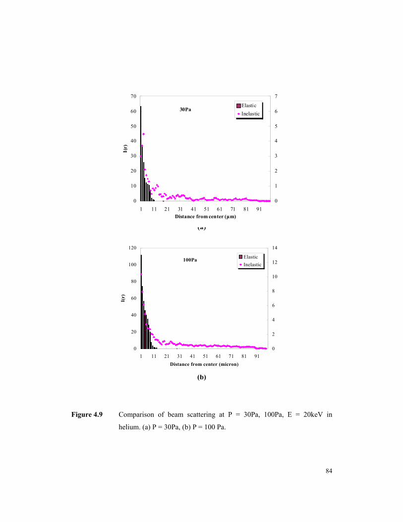
(a)

30Pa

0

10

20

30

40

50

60

70

1 11 21 31 41 51 61 71 81 91Distance from center (µm)

I(r)

0

1

2

3

4

5

6

7

ElasticInelastic

(b)

100Pa

0

20

40

60

80

100

120

1 11 21 31 41 51 61 71 81 91Distance from center (micron)

I(r)

0

2

4

6

8

10

12

14

ElasticInelastic

Figure 4.9 Comparison of beam scattering at P = 30Pa, 100Pa, E = 20keV in

helium. (a) P = 30Pa, (b) P = 100 Pa.

84

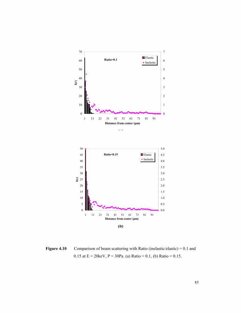
(a)

Ratio=0.1

0

10

20

30

40

50

60

70

1 11 21 31 41 51 61 71 81 91Distance from center (µm)

I(r)

0

1

2

3

4

5

6

7

ElasticInelastic

(b)

Ratio=0.15

0

5

10

15

20

25

30

35

40

45

50

1 11 21 31 41 51 61 71 81 91Distance from center (µm)

I(r)

0.0

0.5

1.0

1.5

2.0

2.5

3.0

3.5

4.0

4.5

5.0

ElasticInelastic

Figure 4.10 Comparison of beam scattering with Ratio (inelastic/elastic) = 0.1 and

0.15 at E = 20keV, P = 30Pa. (a) Ratio = 0.1, (b) Ratio = 0.15.

85

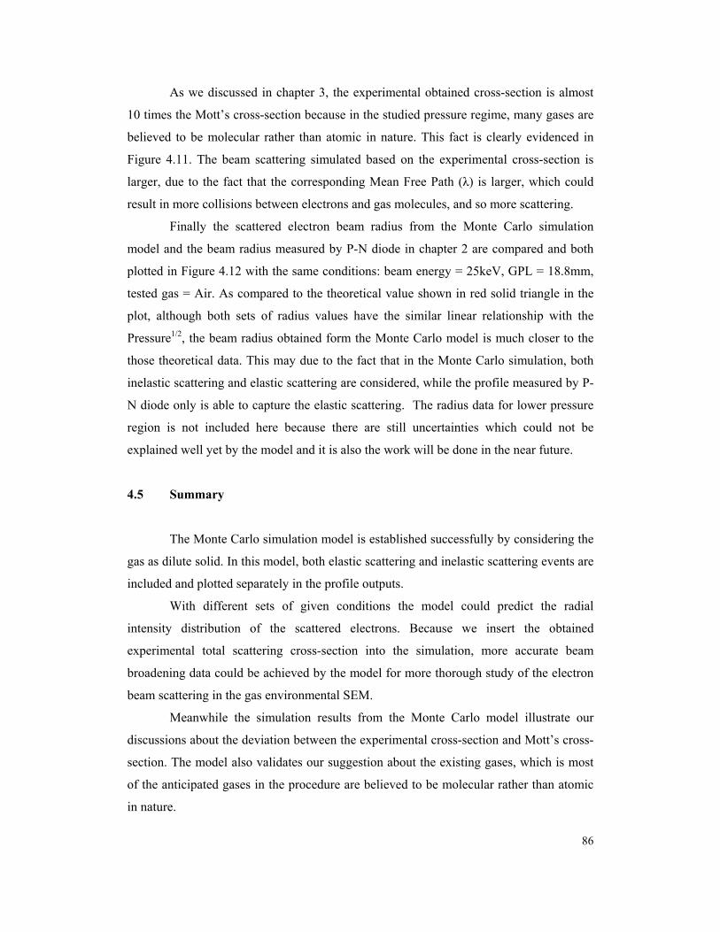
As we discussed in chapter 3, the experimental obtained cross-section is almost

10 times the Mott’s cross-section because in the studied pressure regime, many gases are

believed to be molecular rather than atomic in nature. This fact is clearly evidenced in

Figure 4.11. The beam scattering simulated based on the experimental cross-section is

larger, due to the fact that the corresponding Mean Free Path (λ) is larger, which could

result in more collisions between electrons and gas molecules, and so more scattering.

Finally the scattered electron beam radius from the Monte Carlo simulation

model and the beam radius measured by P-N diode in chapter 2 are compared and both

plotted in Figure 4.12 with the same conditions: beam energy = 25keV, GPL = 18.8mm,

tested gas = Air. As compared to the theoretical value shown in red solid triangle in the

plot, although both sets of radius values have the similar linear relationship with the

Pressure1/2, the beam radius obtained form the Monte Carlo model is much closer to the

those theoretical data. This may due to the fact that in the Monte Carlo simulation, both

inelastic scattering and elastic scattering are considered, while the profile measured by P-

N diode only is able to capture the elastic scattering. The radius data for lower pressure

region is not included here because there are still uncertainties which could not be

explained well yet by the model and it is also the work will be done in the near future.

4.5 Summary

The Monte Carlo simulation model is established successfully by considering the

gas as dilute solid. In this model, both elastic scattering and inelastic scattering events are

included and plotted separately in the profile outputs.

With different sets of given conditions the model could predict the radial

intensity distribution of the scattered electrons. Because we insert the obtained

experimental total scattering cross-section into the simulation, more accurate beam

broadening data could be achieved by the model for more thorough study of the electron

beam scattering in the gas environmental SEM.

Meanwhile the simulation results from the Monte Carlo model illustrate our

discussions about the deviation between the experimental cross-section and Mott’s cross-

section. The model also validates our suggestion about the existing gases, which is most

of the anticipated gases in the procedure are believed to be molecular rather than atomic

in nature.

86

(a)

0

5

10

15

20

25

30

1 11 21 31 41 51 61 71 81 91Distance from beam center (µm)

I(r)

0.0

0.5

1.0

1.5

2.0

2.5

3.0

ElasticInelastic

0

20

40

60

80

100

120

1 11 21 31 41 51 61 71 81 91Distance from center (micron)

I(r)

0

2

4

6

8

10

12

14

ElasticInelastic

(b)

Figure 4.11 Comparison of beam scattering with Mott’s cross-section and

experimental cross-section applied, at E = 20keV and P = 30Pa in

helium. (a) Mott’s cross-section applied in the simulation, (b)

Experimental cross-section applied in the simulation

87

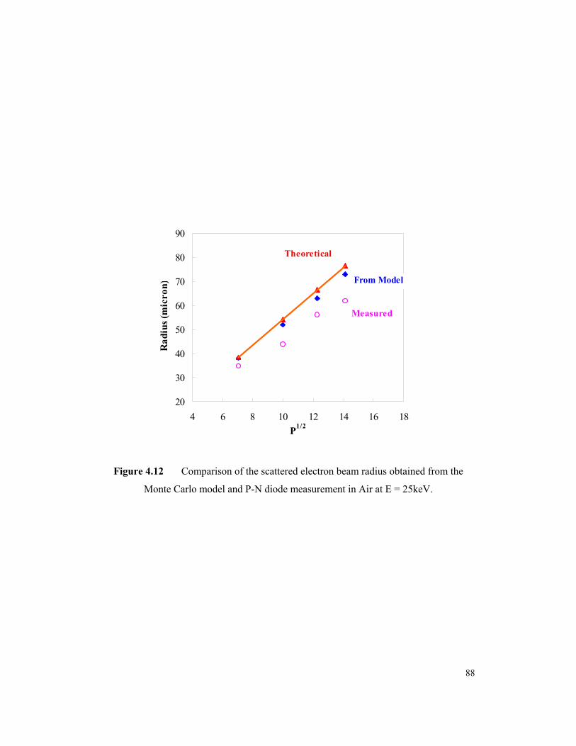
20

30

40

50

60

70

80

90

4 6 8 10 12 14 16 18P1/2

Rad

ius (

mic

ron) From Model

Measured

Theoretical

Figure 4.12 Comparison of the scattered electron beam radius obtained from the

Monte Carlo model and P-N diode measurement in Air at E = 25keV.

88

REFERENCES

89

Adamiak B, Mathieu C: The reduction of the beam gas interactions in the variable

pressure scanning electron microscope with the use of Helium gas, Scanning, Vol.

22, 178-181 (2000)

Berger MJ, Selzer SM: Studies in penetration of charged particles in matter, Nat. Acad

Sci natl Res Council publ, Vol.1133, 205-228 (1964)

Bethe HZ: Theorie des Durchganges schneller Korpuskulerstrahlen durch Material,

Annalen de Phys. (Leipzig), Vol.5, 325-333 (1930)

Bigelow WC: Vacuum Methods in Electron Microscopy in Practical Methods in Electron

Microscopy, Vol.15, Portland Press, London (1994)

Bishop HE: in Use of Monte Carlo Calculations in Electron Prove Microanalysis and

Scanning Electron Microscopy (Eds. KFJ Heinrich, Newbury DE and Yakowitz H

(U.S. Dept. of Commerce/national Bureau of Standards), NBS Special Publication

460, 5 (1976)

Broers AN, Molzen WW, Coumo JJ, Wittle ND: Electron-beam fabrication of 80 Å metal

structures, Appl. Phys. Lett. Vol. 29, 596 (1976)

Cazaux J. 1988

Coburn JW, Winters HF, J. Appl. Phys. Vol. 50, 646 (1987)

Danilatos G.D: Foundations of environmental scanning electron microscopy, Advances in

Electronics and Electron Physics, vol. 71 (1998) 109-250.

Danilatos GD: Foundations of environmental scanning electron microscopy, Advances in

Electronics and Electron Physics, Vol. 71, 109-250 (1988)

Danilatos GD: Theory of gaseous detector device in the environmental, Advances in

Electronics and Electron Physics, Vol. 78, 1-109 (1990a)

Danilatos GD: Fundamentals of environmental SEM, Eleventh Australian Conf. El.

Microsc., University of Melbourne (1990)

Ditmire T: Atomic clusters in ultrahigh intensity light fields, Contemporary Physics, Vol.

38, 5, 315-328 (1997)

Edgerton R.F., Electron Energy-Loss Spectroscopy in the Electron Microscope, Plenum

Press, New York (1996).

Engel VA: Ionized Gases, Clarendon Press, Oxford (1965)

Farley AN, Shah JS: primary considerations for image enhancement in high pressure

scanning electron microscopy. Part 1. J Microsc, Vol. 158, 379-389 (1990a)

90

Farley AN, Shah JS: primary considerations for image enhancement in high pressure

scanning electron microscopy. Part 2. J Microsc, Vol. 158, 390-401 (1990b)

Fiori CE, Swyt CR, Myklebust RL: DTSA – Desk Top Spectrum Analyzer (US Patent

529913) (1992)

Folch A, Servat J, Esteve J, Tejada J, Seco M: High-vacuum versus ‘‘environmental’’

electron beam deposition, J. Vac. Sci. Technol. B 14(4), 2609-2614 (1996)

Gauvin R, David C. Joy, On the Measurement of Total Elastic Cross-Sections in the

ESEN or VPSEM using X-Ray Microanalysis, Microscopy and Microanalysis Vol. 6

(Suppl.2), 788-789 (2000)

Gauvin R, Drouin D: A formula to compute total elastic Mott cross-sections, Scanning,

Vol. 15, 140-150 (1993)

Gauvin R, Griffin B, Nockolds C, Phillips M, Joy, DC: A method to measure the

effective gas path length in the environmental or variable pressure scanning electron

microscope, Scanning, Vol. 24, 171-174 (2002)

Gauvin R, Joy DC: On the measurement of total elastic cross-sections in the ESEM or

VPSEM using X-ray microanalysis, Microscopy and Microanalysis, Vol.6 (Suppl.2),

788-789 (2000)

Gauvin R, L’Esperance G, St-Laurent S: Quantitative X-ray Microanalysis of Spherical

inclusions embedded in a matrix using a SEM and Monte Carlo simulations,

Scanning, Vol. 14, 37-48 (1992)

Gauvin R: Some theoretical considerations on X-ray microanalysis in the environmental

or variable pressure scanning electron microscope, Scanning, Vol.21, 6, 388 (1999).

Gillen G, Wight S, Bright D, Herne T: Quantitative secondary ion mass spectrometry of

self-assembled monolayer film for electron beam dose mapping in the environmental

scanning electron Microscope, Scanning, Vol. 20, 404-409 (1998)

Goldstein JI, Costley JL, Lorimer GW, Reed SJB, Scanning Electron Microscopy, Vol. I,

315 (1977)

Goldstein JI, Newbury DE, Echlin P, Joy DC, Romig AD Jr, Lyman CE, Fiori C, Lifshin

E: Scanning Electron Microscopy and X-ray microanalysis, Plenum Press, New York

(1992)

Hebbard DF, Wilson PR: Austral. J. Phys., Vol. 8, 90 (1955)

Joy DC, Luo S: An empirical stopping power relationship for low-energy electrons,

Scanning, Vol.11, 176-180 (1989)

91

Joy DC: Modeling the electron-gas interaction in low vacuum SEMs, Microscopy and

Microanalysis, 468-469 (1996)

Joy DC: Modeling the electron-gas interaction in low-vacuum SEMs, Microsc Microanal

(Eds. Bailey, Corbett, Dimlich, Micheal, Zaluzec) San Fancisco Press, 836-837

(1996)

Joy DC: Monte Carlo Modeling for Electron Microscopy and Microanalysis, OUP: NY,

(1995)

KFJ Heinrich, Newburey DE and Yakowitz H (U.S. Dept. of Commerce/national Bureau

of Standards), NBS Special Publication 46), 5 (1976)

Mathieu C: Principle and application of the variable pressure SEM, Microscopy Analysis,

Vol. 13, 13-14 (1996)

Mathieu C: The beam-gas and signal-gas interactions in the variable pressure scanning

electron microscope, Scanning Microscopy, Vol.13, No. 1, 23-41 (1999).

Matsui S, Lchihashi T, Mito M: Electron beam induced selective etching and deposition

technology, J. Vac. Sci. Technol. B7 (A5), 1182-1190 (1989)

Matsui S, Mori K, Appl. Phys. Lett. Vol. 51, 646 (1987)

Matsui S, Mori K: New selective deposition technology by electron-beam induced

surface reaction, J. Vac. Sci. Technol, B4, 299 (1986)

McDonald AM et al, Materials World, Vol. 6, no. 7, 399-401 (1998).

Metropolis N: The beginning of the Monte Carlo Method, Los Alamos Science, Special

Issue, 125-130 (1987)

Mohan A, Khanna N, Hwu J, Joy DC: Secondary electron imaging in the variable

pressure scanning electron microscope, Scanning, Vol. 20, 436–441 (1998)

Moncrieff DA, Barker PR, Robinson VNE, Harris LB: Electron scattering by gas in the

scanning electron microscope, J. Phys. D: Appl. Phys., Vol. 12, 481-488 (1979)

Moncrieff DA, Robinson VNE, Harris LB: Charge neutralization of insulating surfaces in

the SEM by gas ionization, J. Phys. D: Appl. Phys., Vol.11, 2315-2325 (1978)

Montgomery DC: Design and Analysis of Experiments, 5th Edition, Wiley & Sons,

(2000)

Newbury DE, Myklebust RL, Analytical Electron Microscopy (Ed. Geiss RH), San

Francisco Press, San Francisco (1981)

Newbury DE, Yakowitz H, Myklebust RL: The NBS Monte Carlo program, in Use of

Monte Carlo Calculations in Electron Prove Microanalysis and Scanning Electron

92

Microscopy (Eds. KFJ Heinrich, Newburey DE and Yakowitz H (U.S. Dept. of

Commerce/national Bureau of Standards), NBS Special Publication 460, 151-164

(1976)

Newbury DE: Modeling electron beam interactions in semiconductors, in SEM

Microcharacterization of Semiconductor (Eds. Holt DE, Joy DC) Academic Press,

London (1989)

Oho E, Asai N, Itoh S: Image quality improvement using helium gas in low voltage

variable pressure scanning electron microscopy, Journal of Microscopy, Vol. 49 (6),

761-763 (2000)

Paul B: Effects of gas pressure on low-pressure electron-beam lithography, Scanning,

Vol. 19, 466-468 (1997)

R.F. Edgerton, Electron Energy-Loss Spectroscopy in the Electron Microscope, Plenum

Press, New York (1996).

Reimer L: Scanning Electron Microscopy, Springer-Verlag, Berlin (1985)

Romer MJ, Araujo D, Garcia R: Energy-loss dependence of inelastic interactions

between high-energy electrons and semiconductors: a model to determine the spatial

distribution of electron-hole pairs generation, Materials Science and Engineering,

Vol.b42, 168-171 (1996)

Schumacher BW: Ontario Research Foundation Physics Research Report No. 6604

(1968)

Smith RC, Schumacher BW, Nucl. Inst. and Methods, Vol. 118, 73 (1974)

Stowe SJ, Robinson VNE: The use of helium gas to reduce beam scattering in high vapor

resource scanning electron microscopy application, Scanning, Vol. 20, 57-60 (1998)

Tang X: Quantitative measurements of charging in a gaseous environment, Microscopy

and Microanalysis, Vol. 8 (Suppl 2), 1540-1541 (2002)

Toth M, Kucheyev SO, Williams JS, Jagadish C, Phillips MR, Li G (2000)

Toth M, Thiel BL, Donald AM, J. Microscopy, Vol.205, 86 (2002)

Wight SA Experimental data and model simulations of beam spread in the environmental

scanning electron microscope, Scanning, Vol. 23, 320-327 (2001)

Wight SA: Beam size in the environmental SEM: A comparison of model and

experimental data. Microscopy Microanalysis (suppl 2) 4, 298-299 (1998)

93

Wight SA: Direct measurement of electron beam scattering in the environmental

scanning electron microscope using phosphor imaging plates. Scanning, Vol. 22,

167-172 (1999)

Yu XR, Hantsche H, J. Electron Spectroscopy and Related Phenomena, Vol.50, 19

(1990)

94

APPENDIX

95

“GASSEM” code wrote in Visual Basic

'This program computes the broadening an electron beam in a gas '(c) Jing He November 2002 'Modified David Joy November 2002 'complaints, bug reports etc to djoy@utk.edu Option Explicit 'declare all variables Dim a_step, inc_energy, tilt, range, b, ga, s_en Dim al, al_a, ak, er, lam_a, sg, sg_a Dim x, y, z, xn, yn, zn Dim center, BS_coeff, e_min Dim two_pi, beam_range, estimate Dim ca, cb, cc, cx, cy, cz Dim nu, cp, sp, an, an_m, an_n, s_tilt, c_tilt Dim h, i, j, k, the_value As Integer Dim plot_test, r_val, rr_val, color_value As Integer Dim traj_num, bs_yield, num, unscattered As Long Dim at_num, at_wht, density, mn_ion_pot, m_t_step, del_E Dim LH_edge, RH_edge, bottom, pressure, the_top Dim plot_scale, center_x, center_y, radial, TOA Dim bbroad, ddum, total_lambda, gas_sigma Dim E(1 To 51) As Single Dim radius(0 To 99) As Single Dim rradius(0 To 99) As Single Dim data_Z(1 To 15) As Single Dim data_A(1 To 15) As Single Dim data_rho(1 To 15) As Single Dim data_Ec(1 To 15) As Single Dim data_MABS(1 To 15) As Single Dim theta, distance, GPL Dim number, XRay_N, dot_density, E_crit Dim no_color, chop, ID Dim FileName As String Private Sub Command1_Click() 'the gas scattering program. Includes inelastic approximation Dim radius1, radius2, radius3, ll, total Dim fraction, test_type 'clear the screen Picture1.Cls 'reset the counters num = 0 bs_yield = 0 unscattered = 0 fraction = 0.1 'ratio of elastic to total cross-section For i = 0 To 99 'zero the inner scale measure radius(i) = 0

96

rradius(i) = 0 Next i 'get the data for this calculation 'incident beam energy inc_energy = Val(Text1.Text) 'get gas path length in mm distance = Val(Text2.Text) 'in mm GPL = distance * 1000 'put in microns 'number of trajectories to run traj_num = Val(Text3.Text) bbroad = 0.9 * traj_num 'gas pressure (in Pa) pressure = Val(Text5.Text) 'experimental gas total cross-section in Mbarns (10^-18cm2) gas_sigma = Val(Text6.Text) 'read the properties of the gas in the column the_value = List1.ListIndex If the_value < 1 Then the_value = 1 If the_value > 14 Then the_value = 14 'and assign the values at_num = data_Z(the_value) at_wht = data_A(the_value) density = at_wht / 22400 'from Gas law density = density * (pressure / 101080) 'pressure in Pa Call Berger_Selzer Call gas_broadening 'get constants get_constants e_min = 0.5 '500eV minimum useful energy 'draw the screen and set up calibration rings Picture1.ScaleMode = 3 'set scale to pixels Picture1.BackColor = QBColor(15) 'white background 'set up the screen for plotting the display center_x = Picture1.ScaleWidth / 2 LH_edge = center_x * 0.1 RH_edge = center_x * 1.95 center_y = Picture1.ScaleHeight / 2 the_top = center_y * 0.15 ' set up the plotting scale based on the estimated broadening 'plot_scale is pixels per micrometer plot_scale = (Picture1.ScaleWidth * 0.75) / (estimate) ' as a first approximation ignore energy losses and compute ' a value for the total MPF from the experimental cross-section

97

total_lambda = 37700000000# / (gas_sigma * pressure) 'lambda in A, sigma in Mbarns inc_energy = Val(Text1.Text) 'reset the random number generator Randomize '****************************************** '****************************************** '******* the Monte Carlo loop ************ While num < traj_num x = 0 y = 0 z = 0 cx = 0 cy = 0 cz = 1 s_en = inc_energy color_value = 14 'distance before first scattering event 'a_step = -Lambda(s_en) * Log(Rnd) * 0.0001 'microns a_step = -total_lambda * Log(Rnd) * 0.0001 'microns zn = a_step 'check the position of the electron now If zn > GPL Then 'this one hits the surface 'Call xyplot(0, 0) 'plot at center unscattered = unscattered + 1 radius(0) = radius(0) + 1 rradius(0) = rradius(0) + 1 GoTo jump2 End If 'reset the coordinates x = 0 y = 0 z = zn 'now start the single scattering loop While s_en > e_min 'a_step = -Lambda(s_en) * Log(Rnd) * 0.0001 'in microns a_step = -total_lambda * Log(Rnd) * 0.0001 'microns 'now test the type of scattering test_type = Rnd If test_type <= fraction Then 'its elastically scattered Call s_scatter(s_en) GoTo next_step Else Call inelastic_scatter(s_en)

98

End If next_step: Call new_coordinates 'now decide what happens next If zn < 0 Then bs_yield = bs_yield + 1 GoTo jump2 End If If zn > GPL Then 'this one hits the surface ll = (GPL - z) / cc 'length of exit vector xn = x + ll * ca 'exit x coordinate yn = y + ll * cb 'exit y coordinate 'Call xyplot(xn, yn) 'plot it radial = Sqr((xn * xn) + (yn * yn)) 'exit radius from axis rr_val = Int(radial) '1 micron annulae If rr_val < 99 Then rradius(rr_val) = rradius(rr_val) + 1# End If r_val = Int(radial * 10) '0.1 micron annular rings If r_val < 99 Then 'no overflow radius(r_val) = radius(r_val) + 1# 'add it End If GoTo jump2: 'finish this trajectory End If 'otherwise go round again Call reset_next_step Wend 'end of the while loop jump2: 'exit point '********************************************** '********************************************** '******** end of the Monte Carlo loop ******** num = num + 1 If (num Mod 100 = 0) Then Randomize End If Wend 'end of the counter Call Plot_radial Call Plot_rradial 'estimate 90% scattering radius ddum = 0 total = 0 For k = 0 To 99 total = total + rradius(k) * (2 * k + 1) Next k

99

total = 0.9 * total 'look for 90% value For k = 0 To 99 ddum = ddum + rradius(k) * (2 * k + 1) If ddum >= total Then GoTo hiccup Next k hiccup: Text4.Text = "skirt= " & (k + 1) & " microns and " & " m= " & 0.01 * Int(100 * unscattered / num) 'and allow the data to be saved to disk if required 'first give it a unique ID ID = Int(1000 * Rnd) If Check1 = 1 Then 'it will be saved FileName = "a:" & "Test" & ID Debug.Print "this file was "; FileName Debug.Print " " 'now write the file Open FileName For Output As #1 'first save the inelastic data at 0.1 micron steps Write #1, "Inelastic data 0.1um steps" Write #1, "*********" For k = 1 To 99 Write #1, (k * 0.1), " ", radius(k) Next k 'then save the elastic data at 1 micron steps Write #1, " " Write #1, "Elastic data 1um steps" For k = 1 To 99 Write #1, k, " ", rradius(k) Next k Close #1 End If End Sub Private Sub Form_Load() 'color the form to look nice FadeForm Me, False, False, True 'load the data table data_Z(1) = 7.2: data_A(1) = 14.5 data_Z(2) = 2: data_A(2) = 4 data_Z(3) = 14: data_A(3) = 28.02 data_Z(4) = 10: data_A(4) = 20.183 data_Z(5) = 12: data_A(5) = 24 data_Z(6) = 18: data_A(6) = 39.948 data_Z(7) = 16: data_A(7) = 32 data_Z(8) = 22: data_A(8) = 44

100

'set up the Materials list List1.AddItem "Choose one" List1.AddItem "Air" List1.AddItem "Helium" List1.AddItem "Nitrogen" List1.AddItem "Neon" List1.AddItem "Water Vapor" List1.AddItem "Argon" List1.AddItem "Oxygen" List1.AddItem "CO2" 'set up the list control List1.ListIndex = 0 'default values for error trap at_num = 6 at_wht = 12.01 density = 2.34 TOA = 30 'detector take-off angle gas_sigma = 1 'cross-section in Mbarns s_tilt = 0 c_tilt = 1 'set up the constant two_pi = 710 / 113 'initialize text windows Text1.Text = 15 'default inc_energy Text2.Text = 10 'default GPL mm Text3.Text = 10000 'default trajectory number Text5.Text = 100 'default pressure 100Pa Text4.Text = "E-beam in Gas October 2002" Text6.Text = 10 center_x = Picture1.ScaleWidth / 2 LH_edge = center_x * 0.1 RH_edge = center_x * 1.95 center_y = Picture1.ScaleHeight / 2 the_top = center_y * 0.15 bottom = center_y * 1.55 plot_test = 0 End Sub Private Sub FadeForm(frm As Form, Red%, Green%, Blue%) Dim SaveScale%, SaveStyle%, SaveRedraw% Dim i&, j&, x&, y&, pixels% 'save current settings SaveScale = frm.ScaleMode SaveStyle = frm.DrawStyle SaveRedraw = frm.AutoRedraw

101

'paint screen frm.ScaleMode = 3 pixels = Screen.Height / Screen.TwipsPerPixelY x = pixels / 64# + 0.5 frm.DrawStyle = 5 frm.AutoRedraw = True For j = 0 To pixels Step x y = 240 - 245 * j / pixels 'can tweak if required If y < 0 Then y = 0 'error trap frm.Line (-2, j - 2)-(Screen.Width + 2, j + x + 3), RGB(-Red * y, -Green * y, -Blue * y), BF Next j 'reset previous settings frm.ScaleMode = SaveScale frm.DrawStyle = SaveStyle frm.AutoRedraw = SaveRedraw End Sub Public Sub gas_broadening() Dim T, E, estimate1, estimate2 'estimate beam broadening using simple model T = 300 'this is room temperature distance = distance * 0.001 'convert to meters E = inc_energy * 1000 'convert keV to eV 'so the estimated beam broadening is estimate1 = 354 * at_num * distance / E estimate2 = estimate1 * Sqr(pressure / T) estimate = estimate2 * Sqr(distance) * 1000000 'converts to microns estimate = Int(estimate) 'tidy up display 'display this value in a text box Text4.Text = "estimated broadening is " & estimate & "um" End Sub Public Sub Berger_Selzer() 'calculates the mean ionization potential 'using the Berger-Selzer fit with atomic number mn_ion_pot = (9.768 * at_num + (58.5 / at_num ^ 0.19)) * 0.001 End Sub Public Sub s_scatter(energy) 'calculates the scattering angles using

102

'the screened Rutherford model Dim R1, al al = al_a / energy R1 = Rnd cp = 1# - ((2# * al * R1) / (1# + al - R1)) sp = Sqr(1# - cp * cp) 'and get the azimuthal scattering angle ga = two_pi * Rnd End Sub Public Sub new_coordinates() 'computes the new coordinates for the electron 'using the scattering angles found earlier 'transforms coordinates back to laboratory frame Dim v1, v2, v3, v4 If cz = 0 Then cz = 0.000001 'error trap an_m = -cx / cz an_n = 1# / Sqr(1 + (an_m * an_m)) 'get the transformation terms v1 = an_n * sp v2 = an_m * an_n * sp v3 = Cos(ga) v4 = Sin(ga) 'get the new direction cosines ca = (cx * cp) + (v1 * v3) + (cy * v2 * v4) cb = (cy * cp) + (v4 * (cz * v1 - cx * v2)) cc = (cz * cp) + (v2 * v3) - (cy * v1 * v4) 'hence the new coordinates are xn = x + a_step * ca yn = y + a_step * cb zn = z + a_step * cc End Sub Public Sub reset_data() 'resets everything for the next step 'first plot the last step Call xyplot(y, z, yn, zn) 'reset the local variables cx = ca cy = cb cz = cc x = xn y = yn z = zn 'and compute the energy loss on that step del_E = a_step * stop_pwr(s_en) * density * 0.00000001

103

s_en = s_en - del_E End Sub Private Function Lambda(inc_energy) 'calculates the elastic MFP al = al_a / inc_energy ak = al * (1# + al) 'giving the cross-section in cm^2 as sg = sg_a / (inc_energy * inc_energy * ak) 'and lambda in angstroms is Lambda = lam_a / sg End Function Private Sub reset_next_step() 'resets everything for the next step 'first plot the last step ' Call xyplot(xn, yn) 'reset the local variables cx = ca cy = cb cz = cc x = xn y = yn z = zn 'and compute the energy loss on that step del_E = a_step * stop_pwr(s_en) * density * 0.0001 s_en = s_en - del_E End Sub Public Sub xyplot(a, b) 'plot the position of the electron as it hits sample Dim px, py, pxa, pya px = center_x + a * plot_scale py = center_y + b * plot_scale Picture1.DrawWidth = 3 Picture1.PSet (px, py), QBColor(12) Picture1.DrawWidth = 1 End Sub Private Sub get_constants() 'computes constants needed by the program al_a = 0.00343 * at_num ^ 0.667

104

'relativistically correct the beam energy er = (inc_energy + 511#) / (inc_energy + 1022#) er = er * er lam_a = at_wht / (density * 6E+23) 'lambda in cm lam_a = lam_a * 100000000# 'put into angstroms sg_a = at_num * at_num * 12.56 * 5.21E-21 * er End Sub Public Function stop_pwr(energy) 'computer stopping power using modified Bethe law 'the result is in keV/gm/cm^2 If energy < 0.05 Then energy = 0.05 stop_pwr = 78500 * at_num * (Log(1.166 * (energy + 0.85 * mn_ion_pot) / mn_ion_pot)) / (at_wht * energy) End Function Public Sub inelastic_scatter(energy) 'computes the inelastic scattering angle assuming a single 'gas ionization event sp = 0.015 / energy ga = two_pi * Rnd End Sub Public Sub Plot_radial() 'plots the radius[rval](0.1um annulae) data to show beam broadening Dim origin_X, origin_Y, volume Dim prz_x, prz_y Dim dummy2, dummy3 Dim cx, cy, cxx, cyy Dim end_of_range As Integer Picture1.Cls ScaleMode = 3 'set scale to pixels Picture1.BackColor = QBColor(11) 'light cyan background 'set up the screen for plotting the display origin_X = LH_edge origin_Y = the_top 'plot the axes Picture1.CurrentX = origin_X Picture1.CurrentY = origin_Y Picture1.DrawWidth = 2 'first mark in the major axes Picture1.Line (LH_edge, the_top)-(RH_edge, the_top), QBColor(0) Picture1.Line (LH_edge, the_top)-(LH_edge, 220), QBColor(0)

105

'then complete the box Picture1.Line (LH_edge, 220)-(RH_edge, 220), QBColor(0) Picture1.Line (RH_edge, 220)-(RH_edge, the_top), QBColor(0) 'finally some horizontal scale markers Picture1.CurrentX = 80 Picture1.CurrentY = 45 Picture1.Print "Bars - 0.1um spacing 10um total width" 'label the display cx = Picture1.ScaleWidth / 2 'scale independent cy = Picture1.ScaleHeight / 2 'first normalize the radial data For k = 1 To 99 radius(k) = radius(k) / (2 * k + 1) Next k 'and smooth For k = 2 To 98 radius(k) = (radius(k - 1) + 2 * radius(k) + radius(k + 1)) / 4 Next k 'now plot the radial intensity data Picture1.DrawWidth = 2 dummy3 = 1 + radius(1) 'value of I(r) at first channel If radius(1) = 0 Then dummy3 = 1 'error trap For k = 1 To 99 prz_x = LH_edge + 2.5 * (k + 1) prz_y = 220 - 200 * radius(k) / dummy3 Picture1.Line (prz_x, 220)-(prz_x, prz_y), QBColor(3) Next k End Sub Public Sub Plot_rradial() Dim ddummy2, ddummy3, prz_x, prz_y 'first normalize the radial data For k = 1 To 99 rradius(k) = rradius(k) / (2 * k + 1) Next k 'and smooth For k = 2 To 98 rradius(k) = (rradius(k - 1) + 2 * rradius(k) + rradius(k + 1)) / 4 Next k 'plot the rradial intensity data (1 um annulae) as dots Picture1.DrawWidth = 3 ddummy3 = rradius(1) 'value of I(r) at first channel If ddummy3 = 0 Then ddummy3 = 1 'error trap For k = 1 To 99

106

prz_x = LH_edge + 2.5 * (k + 1) prz_y = 220 - 200 * rradius(k) / ddummy3 Picture1.PSet (prz_x, prz_y), QBColor(12) Next k End Sub

107

108

VITA

Jing He was born in Taiyuan, Shanxi in P. R. China on Jan. 20, 1974. She spent

eighteen years in her hometown and graduated from high school in 1992 before she went

to Beijing Science and Technology University. She received her B.A. in Material Science

and Engineering in 1996 and continued her passion for Materials engineering in Central

Iron and Steel Research Institute as an assistant engineer.

She came to United States on Christmas 1999 and started her graduate school in

University of Tennessee from fall 2000. Since then she has been working in the EM lab

of University as a research assistant. Under the instruction of Dr. David Joy she has been

totally fascinated by the electron microscopy field, where she can always see things that

never seen before. With her passion and hard work for her research, she received the

Microbeam Analysis Society Distinguished Scholar Award in 2002.

In May 2003 she graduated from University of Tennessee with her M. S. in

Material Science and Engineering and a Minor degree in Statistics.