A Stochastic Model for a Delayed Product Customization

1

40th Anniversary Volume,

IAPQR, 2013

A Stochastic Model for a Delayed Product Customization

Thomas Ngniatedema* and Srinivas R. Chakravarthy

**

*Department of Business Administration

**Department of Industrial and Manufacturing Engineering

Kettering University, Flint, MI-48504, USA

ABSTRACT

Postponement, also known as delayed differentiation, is a strategy used by some firms in

supply chain to delay the differentiation of a product until a latest possible point closer to

consumption (via demands for the product) as a way to compromise between a complete

push system and a complete pull system. The study herein extends Lee and Tang’s

framework for mass customization of products in three different ways. First, the

components coming from the supply side are incorporated in the framework to account

for a possible supply risk. Secondly, we consider a push-pull system in which common

tasks to manufacture two types of products are performed first up to a pre-determined

differentiation point, and arriving demands will trigger the production process to begin

making the final products based on individual customization. Thirdly, we model the

demands to occur according to a Markovian arrival process (MAP), a versatile point

process very useful in practice. We employ simulation to bring out the qualitative nature

of the model under study through illustrative examples.

Key words: Push and Pull systems, Markovian arrival process, supply chain, product

differentiation, and simulation.

1. INTRODUCTION

In today’s global market, increasing competition and customization needs are leading

firms toward mass customization of their products. According to Stanley Davis (1987), the

author of the book Future Perfect, mass customization is one of the ways to achieve low costs

in a production process yet satisfy individual customer preferences for each unique product.

However, the challenge of meeting individual customer preferences is the ability (a) to

accurately forecast the demands of various products, (b) to manage inventories, and (c) to

provide high service for the customers (Lee and Tang 1997; Peters and Saidin 2000).

2

40th Anniversary Volume, IAPQR, 2013

Postponement, also known as delayed differentiation, is a strategy used by some firms in supply

chain as enabler to delay the differentiation of a product until a latest possible point closer to

consumption by the customers (Anand and Girota, 2007; Swaminathan and Lee 2003; Van Hoek,

2001). Postponement is often cited as an effective technique to balance the trade-off between

cost and customer satisfaction in the presence of ever increasing product variety (demanded by

the customers); the pressure for individual customization of products, which calls for flexibility

and quick responsiveness to provide value to the customer; and the shortening of product life

cycle. All of the above mentioned requirements and restrictions rely heavily on very good

forecasting techniques. The complexities involved in accurately gauging customer demands for

customized products, such as demand planning and forecasting have been addressed in the

literature (Lee and Tang 1997; Zinn and Bowersox 1988; Twede et al. 2000; Battezzati and

Magnani 2000; Yang and Burn 2003; Christopher et al. 2007; Yang and Yang 2010).

Postponement is being implemented, for example, in the computer industry where most finished

products although different, share some common components at the beginning of their

production. Firms in this case either produce finished computers based on forecast or they can

customize the computers very late in the production process after demands are observed (Tibben-

Lembke and Bassok 2005). The customization can be as simple as putting different labels on the

computers to more complex ones such as assembling different electrical, electronic and

peripheral components (Feitzinger and Lee 1997).

The literature suggests three common features related to postponement implementation.

First, postponing the final assembly of a product provides major savings to firms as well as the

flexibility to pool common product diversifications in terms of maximizing the usage of

component inventory (Feitzinger and Lee 1997; Graman and Magazine 2002, Pollard et al. 2008;

Ngniatedema 2012; Wang et al. 2012). Secondly, postponement is also accomplished by

keeping inventory at the components’ level to best respond to the customer needs, which

enables firms to commit to the final product customization only after a demand is realized,

resulting in some savings in inventory holding and shortage costs (Tibben-Lembke and Bassok

2005). Because the final customization often takes place only after the demand is observed, the

3

NGNIATEDEMA AND CHAKRAVARTHY

customer’s desires must be quickly translated into the selection of needed components and then

quickly translated into a set of processes, which are integrated rapidly to create the products or

services. The customer in this case may be charged a premium price to cover the cost attached

to a high-speed operation; which may be expensive compared at a slower pace operation.

A delayed product differentiation framework for one market segment in which two

products can be manufactured with N stages was proposed by Lee and Tang (1997). Their

model describes a production process starting with some common operations up to, say, stage k,

which is referred to as the differentiation point, followed by individual customization of each

product from stages (k + 1) through N. Lee and Tang (1997) assume that for a given period,

when information about product demand distribution is known to be normally distributed, the

number of components needed at each stage of the assembly line is directly related to the

average demand of the end products. The study herein extends Lee and Tang’s framework for

mass customization of products in three different ways. First, components coming from the

supply side are incorporated in the framework to account for a possible supply risk. Second, we

consider a push-pull system in which common tasks to both products are performed first up to

the differentiation point k using an (s, S)-type inventory system to store the base (semi-finished)

items to meet the arriving demands for individual customization. As soon as a demand occurs,

the production process in stage k + 1 (and subsequently all stages through N) will be triggered to

begin making the final product. Finally, our model studies a general case where demands occur

according to a Markovian arrival process (MAP). We employ simulation to study the model and

bring out the qualitative nature of the model under study through illustrative examples.

The paper is organized as follows. In Section 2 we present a brief literature review. The

general model description of the postponement in supply chain is described in Section 3 and in

Section 4 we propose a model that is simulated using ARENA. The simulated results are

discussed in Section 5, and concluding remarks and future work are described in Section 6.

4


2. BACKGROUND LITERATURE

The concept of delay product differentiation, first introduced in the marketing literature

by Anderson (1950), has attracted a lot of attention in the research community. Zinn and

Bowersox (1988) describe three different types of postponement used in supply chain. The first

type, time postponement, is used to delay the downstream movement of goods until customer

orders are received. The second type, place postponement, focuses on the storage of goods at

central locations until customer orders are received. Finally, form postponement is used to delay

product customization until customer orders are received. A comprehensive review of the

postponement literature can be found in Swaminathan and Lee (2003) and in Van Hoek (2001).

The form postponement, considered in this paper, is the most relevant type of

postponement. The recent literature in this category considers the case where activities are

performed before the differentiation point based on forecasted demand and semi-finished

products are stored in an inventory, whereas activities performed after the differentiation point

are triggered by customers’ orders (Lee 1987; Robinson 1990; Skipworth and Harrison 2004;

Tagaras and Cohen 1992). Thus, these studies propose solutions to a problem in which

customization takes place after (random) demands are observed.

Other development of delayed product differentiation has been in the area of integrated

supply chain (Anand and Girota 2007; Harrison and Skipworth 2008; Lee 2010; Narasimhan and

Mahapatra 2004; Trentin and Forza 2010; Yang and Burn 2003). Following Narasimhan and

Mahapatra (2004) and Graman and Magazine (2006)’s call for models that can better explain the

performance implications of integration across global supply chain, Choi et al (2012) and Anand

and Girota (2007) developed models to study the performance of a global postponement

implementation. Choi et al (2012) model an optimal postponement strategy under which the

decoupling points for export can be selected with the minimum cost.

In the literature, other authors also analyze the costs and benefits resulting in

implementing a postponement strategy. The studies by Baker et al. (1986), Gerchak and Henig

(1985), Gerchak et al. (1988), and Lee and Tang (1997) explain how major savings can be

5


generated from the ability to delay the assembly operation until after the demands are observed,

and thus benefiting from the risk pooling effect. The risk pooling effect occurs when the

inventory is held at a central location, allowing the demand variance to be combined, resulting in

a lower expected total cost (Eppen 1979). In the supply chain context, Aviv and Federgruen

(2001) emphasize the benefits of inventory reduction and service improvement since holding

inventory of a non-specific product requires less safety stocks as compared to holding inventory

of several specific products.

Although most of these studies suggest that postponement can be a powerful strategy for

improving inventory levels as well as balance the trade-off between costs and customer service,

there are still gaps in the literature to be filled. To fill this void, we build on the model by Lee

and Tang (1997) for delayed product differentiation in three different ways. First, Lee and

Tang’s model does not include a supply risk and the manufacturer does not order raw materials

directly from the supplier. We consider the supply of components at the first stage of the

production process and match the customer demands with these components from the supply

side. Second, we consider a push-pull system through the differentiation point k wherein the

common tasks to both types of products are performed. The arriving demands for individual

customization will trigger the production process (from stages k+1 through N) to begin making

the final products. Thirdly, our model assumes a more versatile point process, namely, MAP for

the demand process. Our model can be studied using matrix-analytic methods (under suitable

assumptions on the processing and lead times) with a very large state space, However, due to

very high dimension of the model, we resort to simulation. Towards this end, we use ARENA

software (see, Kelton et al.). In addition to obtaining some key system performance measures

such as (a) the mean time a demand has to wait for its product to be made and delivered, (b) the

probability that station(s) after the differentiation point will find a stock-out situation (i.e., not

able to start the production to meet a demand due to lack of semi-finished products at the

differentiation point), (c) fraction of demands exceeding the industry standard for waiting, and

(d) the average number of semi-finished items in the inventory, we also study a cost function.

6


3. GENERAL MODEL DESCRIPTION

We consider the assembly of two end products in sequential steps in which

the first k steps are common to both products , where k is the point

(a.k.a. point of differentiation) after which the products assume their unique identities. Figure 1

depicts the assembly network structure used for our study here. There are buffers following each

assembly operation. Note that up to the differentiation point the buffers are used to produce

semi-finished items (to be consumed from stages k+1 through N as and when the demands occur)

up to the base stock level. Beyond this differentiation point the buffers are used to meet the

demands that are already observed.

Demands occur according to a MAP with representation of dimension m. A

brief description of MAP is given below. Production starts at Stage 1 with generic products and

partially finished are passed on to the next station in the sequence for further processing. The

production proceeds on this same manner until the differentiation stage k. The processing from

stage k+1 until the final processing stage is triggered by an arriving demand for the

finished products. We summarize the model assumption below.

Inventory for semi-finished

Processing Stage

1 2 k

M 1 k +1

k +1

- -

-

- -

- Buffer for raw materials M 2

- -

-

MAP

Figure 1: Description of the model

7


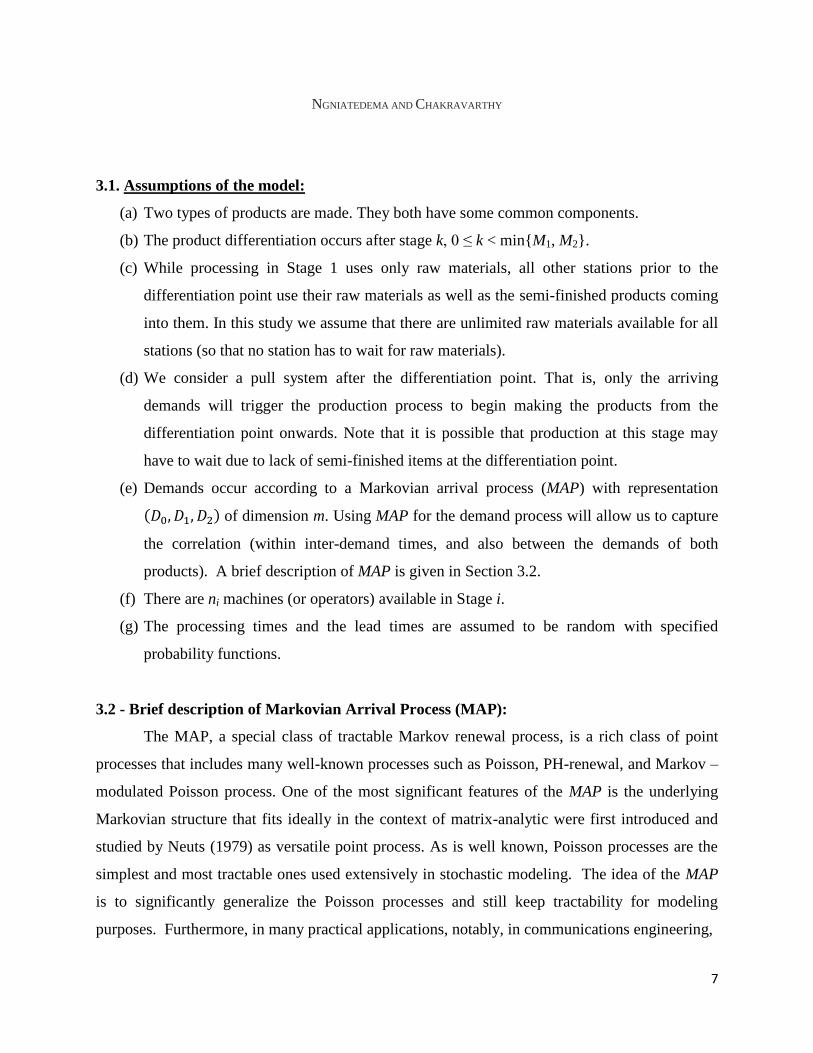
3.1. Assumptions of the model:

(a) Two types of products are made. They both have some common components.

(b) The product differentiation occurs after stage k, 0 ≤ k < min{M1, M2}.

(c) While processing in Stage 1 uses only raw materials, all other stations prior to the

differentiation point use their raw materials as well as the semi-finished products coming

into them. In this study we assume that there are unlimited raw materials available for all

stations (so that no station has to wait for raw materials).

(d) We consider a pull system after the differentiation point. That is, only the arriving

demands will trigger the production process to begin making the products from the

differentiation point onwards. Note that it is possible that production at this stage may

have to wait due to lack of semi-finished items at the differentiation point.

(e) Demands occur according to a Markovian arrival process (MAP) with representation

of dimension m. Using MAP for the demand process will allow us to capture

the correlation (within inter-demand times, and also between the demands of both

products). A brief description of MAP is given in Section 3.2.

(f) There are ni machines (or operators) available in Stage i.

(g) The processing times and the lead times are assumed to be random with specified

probability functions.

3.2 - Brief description of Markovian Arrival Process (MAP):

The MAP, a special class of tractable Markov renewal process, is a rich class of point

processes that includes many well-known processes such as Poisson, PH-renewal, and Markov –

modulated Poisson process. One of the most significant features of the MAP is the underlying

Markovian structure that fits ideally in the context of matrix-analytic were first introduced and

studied by Neuts (1979) as versatile point process. As is well known, Poisson processes are the

simplest and most tractable ones used extensively in stochastic modeling. The idea of the MAP

is to significantly generalize the Poisson processes and still keep tractability for modeling

purposes. Furthermore, in many practical applications, notably, in communications engineering,

8


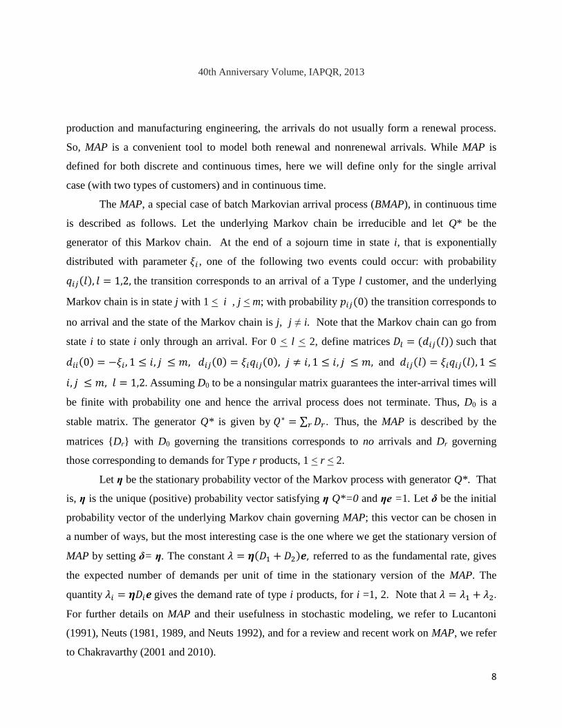
production and manufacturing engineering, the arrivals do not usually form a renewal process.

So, MAP is a convenient tool to model both renewal and nonrenewal arrivals. While MAP is

defined for both discrete and continuous times, here we will define only for the single arrival

case (with two types of customers) and in continuous time.

The MAP, a special case of batch Markovian arrival process (BMAP), in continuous time

is described as follows. Let the underlying Markov chain be irreducible and let Q* be the

generator of this Markov chain. At the end of a sojourn time in state i, that is exponentially

distributed with parameter , one of the following two events could occur: with probability

the transition corresponds to an arrival of a Type l customer, and the underlying

Markov chain is in state j with 1 < i , j < m; with probability the transition corresponds to

no arrival and the state of the Markov chain is j, j ≠ i. Note that the Markov chain can go from

state i to state i only through an arrival. For 0 < l < 2, define matrices such that

and

Assuming D0 to be a nonsingular matrix guarantees the inter-arrival times will

be finite with probability one and hence the arrival process does not terminate. Thus, D0 is a

stable matrix. The generator Q* is given by . Thus, the MAP is described by the

matrices {Dr} with D0 governing the transitions corresponds to no arrivals and Dr governing

those corresponding to demands for Type r products, 1 < r < 2.

Let η be the stationary probability vector of the Markov process with generator Q*. That

is, η is the unique (positive) probability vector satisfying η Q*=0 and ηe =1. Let δ be the initial

probability vector of the underlying Markov chain governing MAP; this vector can be chosen in

a number of ways, but the most interesting case is the one where we get the stationary version of

MAP by setting δ= η. The constant , referred to as the fundamental rate, gives

the expected number of demands per unit of time in the stationary version of the MAP. The

quantity gives the demand rate of type i products, for i =1, 2. Note that .

For further details on MAP and their usefulness in stochastic modeling, we refer to Lucantoni

(1991), Neuts (1981, 1989, and Neuts 1992), and for a review and recent work on MAP, we refer

to Chakravarthy (2001 and 2010).

9


3.3 – Expected Total Cost

In this study, we focus on the stock-out costs, the delay costs, and the inventory costs.

The stock-outs and delays pose serious threats to customer satisfaction in most product

customization as quick response to meeting the demands is critical. In the present study, a stock-

out occurs when the manufacturing of a product after the differentiation point (at the time a

demand occurs) cannot start due to lack of a semi-finished item in Stage 2. Suppose that Ti, i =1,

2, denotes the duration that a demand for Type i product has to wait before it is made. Let wi

denote the norm (or industry standard) for the production time of a demand of a Type i product.

We say that a delay in the production of a demand of Type i product occurs whenever

Defining c1 = inventory holding cost/semi-finished item/unit of time; c2 = cost/unit of

time/stock-out, c3i = cost of delay/unit of time/demand of Type i, (i =1, 2), the expected total cost

(ETC) per unit of time to manufacture and customize the two types of products is obtained as:

where

and denote respectively, the mean number of semi-finished items

(waiting at the end of Stage 2), the probability that an arriving demand of Type j will face a

stock-out situation, the average delay beyond the industry norm of wj that a demand of Type j

product has to face, and the probability that the time to produce the demand for Type j product

will exceed the industry norm.

4. MODEL UNDER STUDY

For this study, we use the assembly of a product that can be assembled in four stages for

our illustrative examples through simulation. We look at the assembly of certain desktop

personal computers (PC) which, based on our conversations with computer professionals, follow

the processing pattern of the general model discussed in Section 3. In this application, the

assembly starts with internal components such as the motherboard, the memory chips, the CPU,

and then the addition of other external components based on the demands.

10


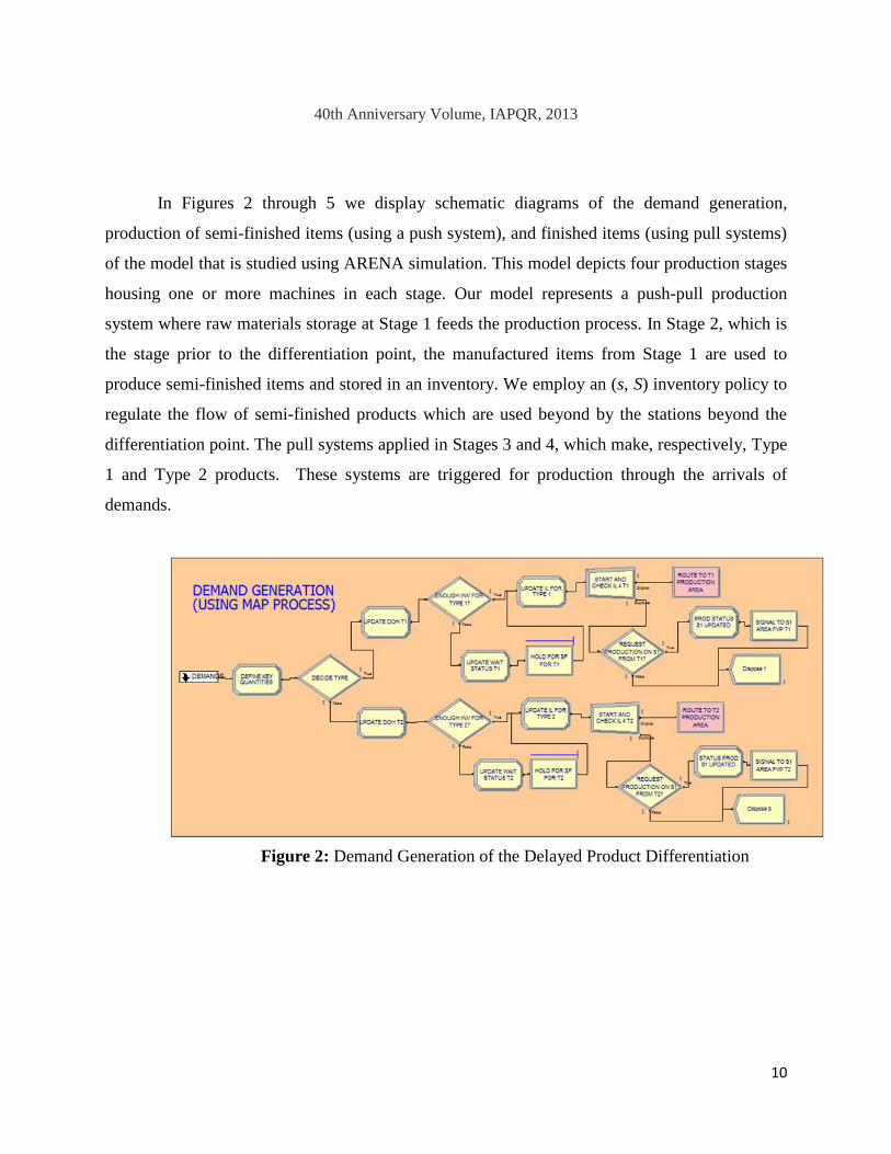
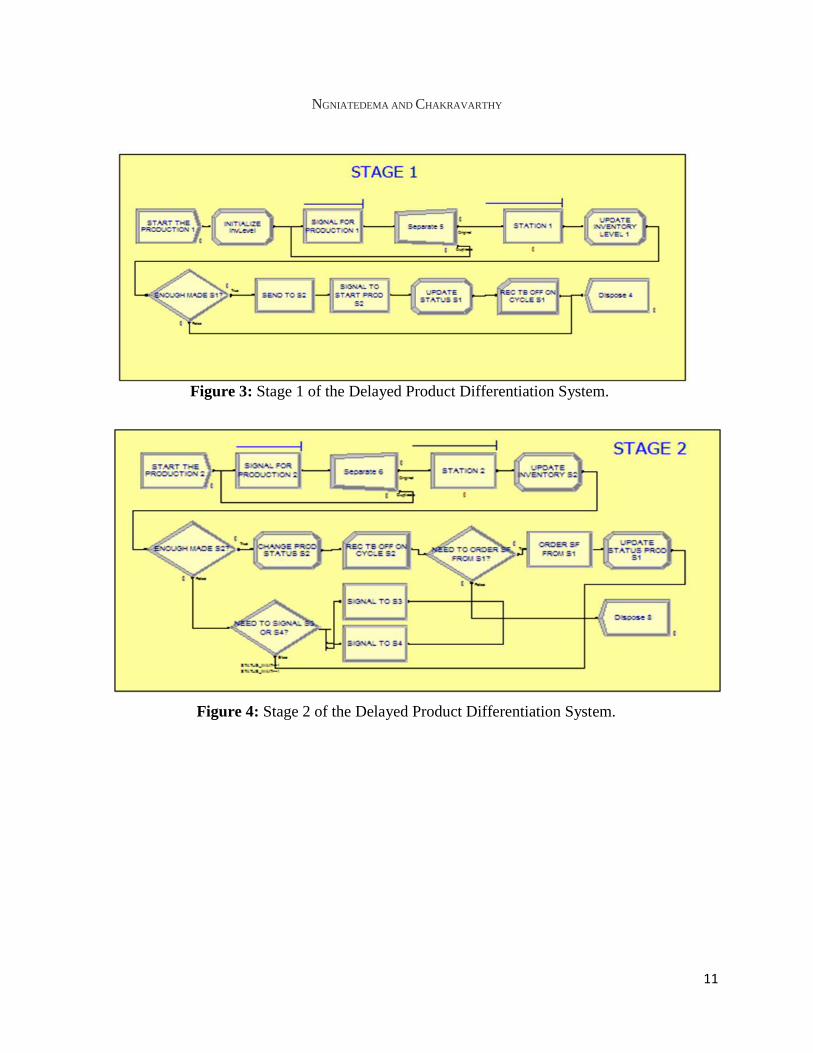
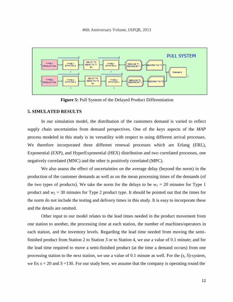
In Figures 2 through 5 we display schematic diagrams of the demand generation,

production of semi-finished items (using a push system), and finished items (using pull systems)

of the model that is studied using ARENA simulation. This model depicts four production stages

housing one or more machines in each stage. Our model represents a push-pull production

system where raw materials storage at Stage 1 feeds the production process. In Stage 2, which is

the stage prior to the differentiation point, the manufactured items from Stage 1 are used to

produce semi-finished items and stored in an inventory. We employ an (s, S) inventory policy to

regulate the flow of semi-finished products which are used beyond by the stations beyond the

differentiation point. The pull systems applied in Stages 3 and 4, which make, respectively, Type

1 and Type 2 products. These systems are triggered for production through the arrivals of

demands.

Figure 2: Demand Generation of the Delayed Product Differentiation

system.

11


Figure 4: Stage 2 of the Delayed Product Differentiation System.

Figure 3: Stage 1 of the Delayed Product Differentiation System.

12


5. SIMULATED RESULTS

In our simulation model, the distribution of the customers demand is varied to reflect

supply chain uncertainties from demand perspectives. One of the keys aspects of the MAP

process modeled in this study is its versatility with respect to using different arrival processes.

We therefore incorporated three different renewal processes which are Erlang (ERL),

Exponential (EXP), and HyperExponential (HEX) distribution and two correlated processes, one

negatively correlated (MNC) and the other is positively correlated (MPC).

We also assess the effect of uncertainties on the average delay (beyond the norm) in the

production of the customer demands as well as on the mean processing times of the demands (of

the two types of products). We take the norm for the delays to be w1 = 20 minutes for Type 1

product and w2 = 30 minutes for Type 2 product type. It should be pointed out that the times for

the norm do not include the testing and delivery times in this study. It is easy to incorporate these

and the details are omitted.

Other input to our model relates to the lead times needed in the product movement from

one station to another, the processing time at each station, the number of machines/operators in

each station, and the inventory levels. Regarding the lead time needed from moving the semi-

finished product from Station 2 to Station 3 or to Station 4, we use a value of 0.1 minute; and for

the lead time required to move a semi-finished product (at the time a demand occurs) from one

processing station to the next station, we use a value of 0.1 minute as well. For the (s, S)-system,

we fix s = 20 and S =130. For our study here, we assume that the company is operating round the

Figure 5: Pull System of the Delayed Product Differentiation

system.

13


clock for a period of ten weeks and take the costs per day (i.e., 1440 minutes) to be:

For our illustrative examples here, three types of processing times are considered. The

numbers of machines in each of the stations for all examples are fixed. These are displayed in

Table 1 below.

Table 1: Distribution of the Processing Time and number of machines at each station

Processing Station 1 2 3 4 5 6

Processing

Time

Example 1 Exp(1) Exp(2) Exp(0.2) Exp(0.2) Exp(0.2) Exp(0.2)

Example 2 Erlang

(0.2,5)

Erlang

(0.2,5)

Erlang

(0.04,5)

Erlang

(0.04,5)

Erlang

(0.04,5)

Erlang

(0.04,5)

Example 3 1 2 0.2 0.2 0.2 0.2

Number of machines 2 4 2 2 2 2

For demand processes, we consider the following five MAP processes with representation

(D0, D1, D2). Recall that D1 and D2, respectively, govern Type 1 and Type 2 demands. Here we

take D1 = D2 = 0.5D, so that Type 1 and Type 2 demands occur with equal probability.

1. Erlang (ERL):

.

2. Exponential (EXP): .

3. HyperExponential (HEX):

.

4. MAP with Negative Correlation (MNC):

.

14


5. MAP with Positive Correlation (MPC):

.

All these five MAP processes are normalized so as to have specific overall demand rate to

be 1. That is, However, these MAPs are qualitatively different in that they have different

variance and correlation structure. Looking only at points at arrivals of demands (irrespective of

whether they are for Type 1 or Type 2), the first three arrival processes correspond to renewal

processes and so the correlation is 0. The arrival process labeled MNC has correlated arrivals

with a correlation value of –0.48891, and the arrivals corresponding to the process labeled MPC

has a positive correlation value of 0.48891. The ratio of the standard deviations of the inter-

arrival times of these five arrival processes with respect to ERL are, respectively, 1, 2.2361,

5.0193, 3.1518, and 3.1518.

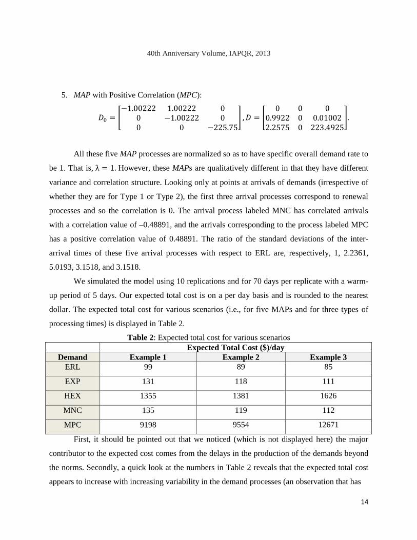
We simulated the model using 10 replications and for 70 days per replicate with a warm-

up period of 5 days. Our expected total cost is on a per day basis and is rounded to the nearest

dollar. The expected total cost for various scenarios (i.e., for five MAPs and for three types of

processing times) is displayed in Table 2.

Table 2: Expected total cost for various scenarios

Expected Total Cost ($)/day

Demand Example 1 Example 2 Example 3

ERL 99 89 85

EXP 131 118 111

HEX 1355 1381 1626

MNC 135 119 112

MPC 9198 9554 12671

First, it should be pointed out that we noticed (which is not displayed here) the major

contributor to the expected cost comes from the delays in the production of the demands beyond

the norms. Secondly, a quick look at the numbers in Table 2 reveals that the expected total cost

appears to increase with increasing variability in the demand processes (an observation that has

15


been noticed in other contexts of stochastic modeling in the literature). Thirdly, the effect of

correlation (especially the positive one) appears to be significant indicating that one should not

ignore correlation in practice.

Our next focus is the mean time to produce the demands of each type of product. That is,

we look at the average time it takes to produce the items demanded by the customers from the

time they are requested. The mean production times of the demands as well as their 95% half-

width values (based on 10 replicates) for each type of product for various scenarios are displayed

in Table 2.

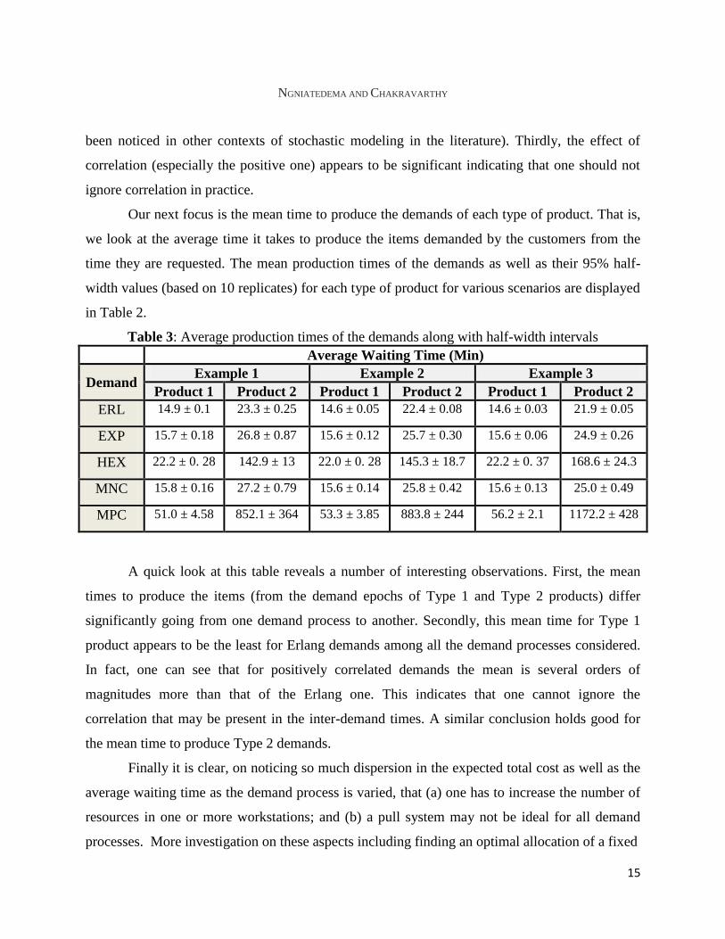
Table 3: Average production times of the demands along with half-width intervals

Average Waiting Time (Min)

Demand Example 1 Example 2 Example 3

Product 1 Product 2 Product 1 Product 2 Product 1 Product 2

ERL 14.9 ± 0.1 23.3 ± 0.25 14.6 ± 0.05 22.4 ± 0.08 14.6 ± 0.03 21.9 ± 0.05

EXP 15.7 ± 0.18 26.8 ± 0.87 15.6 ± 0.12 25.7 ± 0.30 15.6 ± 0.06 24.9 ± 0.26

HEX 22.2 ± 0. 28 142.9 ± 13 22.0 ± 0. 28 145.3 ± 18.7 22.2 ± 0. 37 168.6 ± 24.3

MNC 15.8 ± 0.16 27.2 ± 0.79 15.6 ± 0.14 25.8 ± 0.42 15.6 ± 0.13 25.0 ± 0.49

MPC 51.0 ± 4.58 852.1 ± 364 53.3 ± 3.85 883.8 ± 244 56.2 ± 2.1 1172.2 ± 428

A quick look at this table reveals a number of interesting observations. First, the mean

times to produce the items (from the demand epochs of Type 1 and Type 2 products) differ

significantly going from one demand process to another. Secondly, this mean time for Type 1

product appears to be the least for Erlang demands among all the demand processes considered.

In fact, one can see that for positively correlated demands the mean is several orders of

magnitudes more than that of the Erlang one. This indicates that one cannot ignore the

correlation that may be present in the inter-demand times. A similar conclusion holds good for

the mean time to produce Type 2 demands.

Finally it is clear, on noticing so much dispersion in the expected total cost as well as the

average waiting time as the demand process is varied, that (a) one has to increase the number of

resources in one or more workstations; and (b) a pull system may not be ideal for all demand

processes. More investigation on these aspects including finding an optimal allocation of a fixed

16


number of resources to various stations is under study and the results of this study will be

addressed elsewhere.

6. CONCLUDING REMARKS AND FUTURE WORK

The demand process is known to drive the managerial decisions when it comes to

balancing the trade-off between the most two important dimensions: cost and customer

satisfaction, in mass customization where the product diversity tends to be high.

This research emphasized the importance of delayed product differentiation for product

customization in supply chain where the demands occur according to a Markovian arrival

process. Postponement was used to compromise between a complete push system and a complete

pull system. We extended Lee and Tang’s framework for mass customization of products in

three different ways. First, the supplies of raw materials were incorporated into the framework to

account for supply risk. Second, we considered a push-pull system in which common tasks to

both products are performed first up to a pre-determined differentiation point, and the arriving

demands for individual customization triggers the production process to begin making the final

products. Using a versatile point process to model the demands we employed a simulation

method to bring out the qualitative nature of the model under study through illustrative examples.

Using five scenarios for the demand processes, we showed through simulation, the effect of the

type of demand processes on the average total operating costs as well as on the average

production times to meet the demands.

Our simulation results clearly indicated how the type of the customer demand process in

the context of a delayed differentiation approach has an impact on the key system measures and

the expected total operating cost. The ability to compare the expected total operating cost and the

mean time to produce the items of the demands of either type of the products provides a better

insight that is valuable to the stakeholder. Also, our study showed that when the inter-demand

times have a reasonably small variation (like in Erlang case), a pull system beyond the

differentiation point is appropriate as it has no inventory to store and also appears to have less

mean production time to meet the demands. However, if the inter-demand times have either a

large variation (such as hyperexponential) or have correlation between two successive ones (like

17


MPC demand process), a pull system may yield a higher mean production time to meet the

demands. A combination of a push and pull system may be a way to accomplish a smaller mean

wait time and hence a smaller expected total cost.

In practice, supply chains tend to suffer from uncertainties, and postponement is one of

the ways to minimize the effect of too much inventory or too much stock-outs. In our study we

made several assumptions, some of which represent limitations and therefore present

opportunities for future research. First, we assumed that there is an unlimited supply of raw

materials in Stage 1 that feeds the production process down the road. Further studies need to be

conducted to relax this assumption along with the possibility of having a stock-out at the

beginning of the production process. While we employed an (s, S)-type inventory policy in this

study, other policies are worth considering and it would be of interest to study the effect of the

inventory parameters on the expected total operating cost. Finally, we can extend the current set

up of four-stations for each of two types of products to several-stations case. Currently, we are

exploring different options to the one presented here and the results of the study will be reported

elsewhere.

REFERENCES

Anand, K.S., Girota, K. (2007). “The strategic perils of delayed differentiation”, Management

Science 53 (5), 697–712.

Alderson, W. (1950), “Marketing efficiency and the principle of postponement”, Cost and

Profit Outlook, 3, 15–18.

Aviv, Y. and Federgruen, A. (2001), “Design for postponement: a comprehensive

characterization of its benefits under unknown demand distributions”, Operation

Research, 49(4), 578–598.

Baker, K.R., Magazine, J.R. and Nuttle, H.W. (1986), “The effect of commonality on safety

stock in a simple inventory model, Management Science 32, 982–988.

Battezzati, L. and Magnani R. (2000), "Supply Chains for FMCG and Industrial Products in

Italy: Practices and the Advantages of Postponement", International Journal of Physical

Distribution & Logistics Management. 30(5), 413 – 424.

Chakravarthy, S.R. (2001), “The batch Markovian arrival process: A review and future work.

Advances in Probability Theory and Stochastic Processes”, Eds., A. Krishnamoorthy et

al., Notable Publications Inc., NJ, 21-39

Chakravarthy, S.R. (2010), “Markovian Arrival Processes. Wiley Encyclopedia of Operations

18


Research and Management Science”, Published Online: 15 JUN 2010.

Choi, K., Narasimhan, R. and Kim, S. W. (2012), Postponement strategy for international

transfer of products in a global supply chain: A system dynamics examination. Journal of

Operations Management, 30 (6), 167–179.

Christopher, M., Jia, F., Khan, O., Mena, C., Palmer, A., Sandberg, E. (2007), "Global sourcing

and logistics", Department for Transport, Cranfield School of Management, Cranfield,

Logistics project number LP 0507.

Davis, S. M., “Future Perfect”. Addison-Wesley Publishing. Reading, MA, 1987.

Eppen G.D. (1979), Effects of centralization on expected costs in a multi-location newsboy

problem. Management Science, 25(5):498–501.

Feitzinger, E. and Lee, H.L. (1997), “Mass customization at Hewlett Packard: the power of

postponement.” Harvard Business Review, 75(1), 116-121.

Graman G.A. and Magazine M.J. (2002), A Numerical analysis of capacitated postponement.

Production and Operations Management, 11(3), 340-357.

Gerchak, Y. and Henig M. (1985), “An inventory model with component commonality”,

Operations Research Letters, 5(3), 157–160.

Gerchak, Y., Magazine, M. and Gamble A.B. (1988), Component commonality with service

level requirements, Management Science 34 (6), 753–760.

Harrison, A. and Skipworth, H. (2008), “Implications of Form Postponement to

Manufacturing: a Cross Case Comparison”, International Journal of Production Research.

46(1):173-195.

Jensen P.A. and Bard J.F. (2003), "Operations Research Models and Methods", John Wiley &

Sons, New York.

Kelton, W.D., Sadowski, R.P., Swets, N.B. (2010), “Simulation with ARENA”, Fifth ed.,

McGraw-Hill, New York.

Lee, L.H. (2010), Global trade process and supply chain management. In: Sodhi, M.S.,

Tang, C.S. (Eds.), A Long View of Research and Practice in Operations Research

and Management Science: The Past and the Future, International Series in Operations

Research & Management Science, vol. 148. Springer, Massachusetts.

Lee H., Billington C., and Carter B. (1993), Hewlett-Packard gains control of inventory and

service through design for localization, Interfaces, 23 (4),1–11.

Lee H. (1987), “A multi-echelon inventory model for repairable items with emergency lateral

transshipments”, Management Science, 33(10), 1302–1316.

Lee, H. and Tang, C.S. (1997), “Modelling the costs and benefits of delayed product

differentiation”, Management Science, 43(1), 40–53.

Lucantoni, D.M. (1991), “New results on the single server queue with a batch Markovian arrival

process. Stochastic Models”, 7, 1-46.

Narasimhan, R. and Mahapatra, S. (2004), “Decision Models in Global Supply Chain

Management”, Industrial Marketing Management. 33(1), 21–27.

Neuts, M.F.(1979), “A versatile Markovian point process”, J. Appl. Prob., 16, 764-779.

19


Neuts, M.F. (1981), “Matrix-Geometric Solutions in Stochastic Models: An Algorithmic

Approach”, The Johns Hopkins University Press, Baltimore, MD [1994 version is Dover

Edition].

Neuts, M.F. (1989), “Structured Stochastic Matrices of M/G/1 type and their Applications”,

Marcel Dekker, NY.

Neuts, M.F. (1992), “Models based on the Markovian arrival process”, IEICE Transactions on

Communications, E75B, 1255-1265.

Ngniatedema, T. 2012: “A Mass Customization Information Systems Architecture

Framework”, Journal of Computer Information Systems. 52(3), 60-70.

Peters, L. and Saidin, H. (2000), “IT and the mass customization of services: the challenge of

Implementation”, International Journal of Information Management. 20(2), 103–119.

Pollard, D., Chuo, S. and Lee B. (2008), “Strategies for mass customization”, Journal of

Business and Economics Research. 6(7), 77-86

Robinson L.(1990), “Optimal and approximate policies in multi-period multi-echelon inventory

models with transshipments”, Operations Research 23 (2), 278–295.

Skipworth, H. and Harrison, A. (2004), “Implications of form postponement to manufacturing: a

case study”, International Journal of Production Research, 42(10), 2063–2081.

Swaminathan, J.M. and Lee, H.L.(2003), “Design for postponement. In Supply Chain

Management”—Handbook in OR/MS, edited by S. Graves and T. de Kok, 11, 199–226.

Tagaras, G. and Cohen M. (1992), “Pooling in two-location inventory systems with non-

negligible lead times”, Management Science, 38 (8), 1067–1078.

Tibben-Lembke R.S. and Bassok Y. (2005), “An inventory model for delayed customization: A

hybrid approach”, European Journal of Operational Research, 165(3) 748–764.

Trentin, A.and Forza, C. (2010), “Design for Form Postponement: Do Not Overlook

Organization Design”, International Journal of Operations & Production Management.

30 (4), 338–364.

Twede, D. T., Clarke, R. H. and Tailt, J. A. (2000), “Packaging Postponement: A Global

Packaging Strategy”, Packaging Technology and Science. 13(3), 105–115.

Van Hoek, R. I. (2001), “The Rediscovery of Postponement: A Literature Review and Directions

for Future Research”, Journal of Operations Management. 19(2), 161–184.

Wang, X. Xie, Z. and Guan, Z. (2012), “Partial Postponement Strategy: Application in

Automobile Manufacturers”, Advanced Materials Research. 443-444(296), 296-301.

Yang, B. and Burns, N. D. (2003), “The Implications of Postponement for the Supply Chain”,

International Journal of Production Research. 41(9), 2075–2090.

Yang, B. and Yang, Y. (2010), “Postponement in Supply Chain Risk Management: A

Complexity Perspective”, International Journal of Production Research, 48(7), 1901–12.

Zinn, W. and Bowersox, D.J. (1988), “Planning physical distribution with the principle of

Postponement”, Journal of Business Logistics. 19(2), 117–136.

A Stochastic Model for a Delayed Product Customization

Documents

Transcript of A Stochastic Model for a Delayed Product Customization