Edinburgh Research Explorer

A statistical framework to quantify spatial variation in channelgradients using the integral method of channel profile analysis

Citation for published version:Mudd, SM, Attal, M, Milodowski, D, Grieve, SWD & Valters, DA 2014, 'A statistical framework to quantifyspatial variation in channel gradients using the integral method of channel profile analysis', Journal ofGeophysical Research: Earth Surface, vol. 119, no. 2, pp. 138–152. https://doi.org/10.1002/2013JF002981

Digital Object Identifier (DOI):10.1002/2013JF002981

Link:Link to publication record in Edinburgh Research Explorer

Document Version:Publisher's PDF, also known as Version of record

Published In:Journal of Geophysical Research: Earth Surface

General rightsCopyright for the publications made accessible via the Edinburgh Research Explorer is retained by the author(s)and / or other copyright owners and it is a condition of accessing these publications that users recognise andabide by the legal requirements associated with these rights.

Take down policyThe University of Edinburgh has made every reasonable effort to ensure that Edinburgh Research Explorercontent complies with UK legislation. If you believe that the public display of this file breaches copyright pleasecontact openaccess@ed.ac.uk providing details, and we will remove access to the work immediately andinvestigate your claim.

Download date: 30. Jan. 2022

A statistical framework to quantify spatial variation in channelgradients using the integral method of channel profile analysis

Simon M. Mudd,1 Mikaël Attal,1 David T. Milodowski,1 Stuart W. D. Grieve,1

and Declan A. Valters 1

Received 12 September 2013; revised 5 December 2013; accepted 6 December 2013.

[1] We present a statistical technique for analyzing longitudinal channel profiles. Ourtechnique is based on the integral approach to channel analysis: Drainage area is integratedover flow distance to produce a transformed coordinate, χ, which has dimensions of length.Assuming that profile geometry is conditioned by the stream power law, defined asE=KAmSnwhere E is erosion rate, K is erodibility, A is drainage area, S is channel gradient,and m and n are constants, the slope of a transformed profile in χ-elevation space shouldreflect the ratio of erosion rate to channel erodibility raised to a power 1/n; this quantity isoften referred to as the channel steepness and represents channel slope normalized fordrainage area. Our technique tests all possible contiguous segments in the channel networkto identify the most likely locations where channel steepness changes and also identifies themost likely m/n ratio. The technique identifies locations where either erodibility or erosionrates are most likely to be changing. Tests on a simulated landscape demonstrate that thetechnique can accurately retrieve both the m/n ratio and the correct number and location ofsegments eroding at different rates where model assumptions apply. Tests on naturallandscapes illustrate how the method can distinguish between spurious channel convexitiesdue to incorrect selection of the m/n ratio from those which are candidates for changingerodibility or erosion rates. We also show how, given erosion or uplift rate constraints, themethod can be used to constrain the slope exponent, n.

Citation: Mudd, S. M., M. Attal, D. T. Milodowski, S. W. D. Grieve, and D. A. Valters (2014), A statistical framework toquantify spatial variation in channel gradients using the integral method of channel profile analysis, J. Geophys. Res. EarthSurf., 119, doi:10.1002/2013JF002981.

1. Introduction

[2] Fluvial incision is one of the fundamental geomorphicprocesses that drive the evolution of eroding landscapes.Early geomorphologists recognized that channel gradientsvary systematically with drainage area and reasoned that allelse being equal, steeper channels should erode more rapidly[e.g., Davis, 1899]. This reasoning has motivated much re-search into bedrock rivers because it raises the possibilityof using channel gradients to infer erosion rates. Howardand Kerby [1983] proposed that in bedrock rivers, erosionshould be proportional to the power the river expends on itsbed. Stream power depends on the flux of water in the chan-nel, which is a function of drainage area, and the channel gra-dient. Thus, in areas of uniform lithology and climate acharacteristic relationship between slope and drainage areacan be expected for a given erosion rate. Later workers foundthat the geometry of bedrock river profiles is broadly consis-tent with a class of models similar to that first suggested by

Howard and Kerby [1983] and extended by others [e.g.,Seidl and Dietrich, 1992; Howard, 1994]. Subsequently,so-called slope-area analysis has frequently been used to re-veal patterns of erosion and, by inference, tectonic activityin channel networks [Stock and Montgomery, 1999; Kirbyand Whipple, 2001; Kirby et al., 2003; Snyder et al., 2003;Wobus et al., 2006; Miller et al., 2007; DiBiase et al.,2010; Kirby and Ouimet, 2011; Kirby and Whipple, 2012].[3] Topographic data are, however, inherently noisy. The

noise arises from uncertainties in the data collection [e.g.,Hodgson and Bresnahan, 2004; Eckert et al., 2005] but alsofrom the natural heterogeneity that characterizes geomorphicsystems: Channel beds are often uneven and local topo-graphic features (e.g., steps in a river profile due to fracturesin bedrock; accumulation of boulders at the base of a rockface) may not reflect regional erosion rates. Because slopeis the spatial derivative of topography, slope data containyet more noise, so analysis of channel slopes requires a de-gree of smoothing and data binning that may reveal broadpatterns in the landscape [e.g., Wobus et al., 2006] but willfail to identify subtler spatial and/or temporal variations inerosion rates. Perron and Royden [2013], building on earlierwork by Royden et al. [2000], offered an elegant solution tothis problem by using an integral transformation of the riverprofile’s horizontal coordinate into a variable χ (chi), whichhas units of distance but accounts for longitudinal variations

1School of GeoSciences, University of Edinburgh, Edinburgh, UK.

Corresponding author: S. M. Mudd, School of GeoSciences, Universityof Edinburgh, Drummond St., Edinburgh EH8 9XP, UK.(simon.m.mudd@ed.ac.uk)

©2013. American Geophysical Union. All Rights Reserved.2169-9003/14/10.1002/2013JF002981

1

JOURNAL OF GEOPHYSICAL RESEARCH: EARTH SURFACE, VOL. 119, 1–15, doi:10.1002/2013JF002981, 2014

in drainage area. Plots of channel elevations against thistransformed length variable (or “chi plots;” Perron andRoyden [2013]) can be used to reveal the steepness of riverreaches without having to calculate channel slopes. Thisform of channel analysis, which Perron and Royden [2013]have called the integral method, has a number of attractivefeatures. Critically, as the integral method does not involvedifferentiation, there is a significant reduction in noiserelative to slope-area analysis. Consequently, estimates ofchannel steepness using the integral method have reduceduncertainty, and there is no longer a requirement to log-binthe data, which permits analysis of much finer details in thechannel network (see Perron and Royden [2013] for a fulldiscussion of the advantages and potential drawbacks of thismethod). The integral method has the potential to provideprecise quantitative information about erosion rates and theirspatial and temporal variations over areas for which topo-graphic data are available, which could then be used to gaininsight into the spatial and temporal variations in the con-trolling external forces, namely tectonics and climate. Toachieve this, however, a transparent, robust, and objectivemethod for discriminating between river reaches with differ-ent normalized steepness values must exist. In the followingsections we (i) outline the theoretical principles of the inte-gral method and discuss its application in steady state andtransient and/or heterogeneous landscapes, (ii) develop a sta-tistical framework with which to apply this method, and (iii)demonstrate the utility of this technique using a series ofexamples based on both numerical simulations and analysisof real landscapes.

2. The Integral Method of ChannelProfile Analysis

[4] The evolution of a channel experiencing uplift anderosion driven by stream power can be stated as follows[e.g., Howard and Kerby, 1983;Whipple and Tucker, 1999]:

∂z∂t

¼ U x; tð Þ þ K x; tð ÞAm ∂z∂x

��������n

; (1)

where z (dimensions length; dimensions are hereafter denotedin brackets and abbreviated as [L]ength, [M]ass, and [T]ime) isthe elevation of the channel, x [L] is a longitudinal coordinate,A [L2] is the drainage area, U [L T�1] is the uplift rate, andK [T�1 L(1�2m)] is an erodibility coefficient which encapsu-lates the influence of climate, lithology, and other factors.The exponentsm and n are empirically derived coefficients, al-though values of n have been proposed based on the mechan-ics of bedrock incision, ranging between 2/3 and 7/3 [Whippleet al., 2000]. Both U and K may be functions of space andtime, and K may also be a function of sediment supply [e.g.,Sklar and Dietrich, 2004; Cowie et al., 2008; Hobley et al.,2011] and incorporate the influence of an erosion thresholdand channel width adjustment [e.g., Snyder et al., 2003;Lague, 2010; Attal et al., 2011]. The stream power approach,its limitations, and alternatives are reviewed by Lague[2013]. The integral method devised by Perron and Royden[2013] (see also Royden and Perron [2013]) is based on theassumption that the evolution of the studied channels can bedescribed by equation (1).

2.1. Chi Analysis: Steady State Example

[5] To introduce the integral method of channel analysis,we consider a simplified system in which K and U are con-stant in space and time, and uplift is balanced by erosion suchthat the elevation of the channel does not change in time(a so-called steady state channel):

dz

dx

�������� ¼ U

K

� �1=n

A xð Þ�m=n: (2)

[6] Equation (2) implies that plotting slope (|dz/dx|) againstdrainage area in log-log space should produce a straight linewith a gradient-m/n (often referred to as the channel concav-ity or concavity index, e.g., Whipple and Tucker [1999]),whereas the vertical position of the line in the plot shouldbe indicative of the ratio of uplift to erodibility (U/K) raisedto the power 1/n. This relationship has been exploited by nu-merous authors to infer both erodibility [e.g., Stock andMontgomery, 1999] and tectonic uplift rates (see reviewsby Wobus et al. [2006] and Kirby and Whipple [2012]).However, the noise inherent in slope data requires smoothingand averaging of slope-area data before they can be used tomake inferences about erosion or tectonics [Wobus et al.,2006]. In addition, slope-area data tend to show discontinu-ities, due to the fact that drainage area does not increasesteadily downstream: Abrupt increases in drainage area attributary junctions cause clustering of the data and createlarge uncertainties on regressions. An alternative approachis to avoid differentiation and thus eliminate the main sourceof noise [e.g., Royden et al., 2000; Pritchard et al., 2009;Perron and Royden, 2013]. One means of retaining drainagearea and elevation information is to separate and then inte-grate equation (2) [e.g., Royden et al., 2000; Harkins et al.,2007; Perron and Royden, 2013]:

∫dz ¼ ∫U

KAm

� �1=n

dx: (3)

[7] In a system in which K and U are constant in space andtime, equation (3) may be integrated upstream from somebase level at xb to arrive at

z xð Þ ¼ z xbð Þ þ U

KAm0

� �1=n

χ; (4a)

where

χ ¼ ∫xxbA0

A xð Þ� �m=n

dx; (4b)

and A0 is a reference drainage area, introduced to ensure theintegrand in equation (4b) is dimensionless. The transformedcoordinate, χ, has dimension of length and the elevation, z(x),is a linear function of χ in this situation (K and U constant inspace and time) according to equation (4a). Thus, a channelthat obeys equation (2) will appear as a straight line in a chiplot, and the slope of the line will be a function of the upliftto erodibility ratio (U/K) raised to the power 1/n. Perronand Royden [2013] pointed out several additional featuresthat make chi plots an attractive alternative to slope-areaplots. Importantly, the coordinate χ depends on the m/n ratio,

MUDD ET AL.: CHANNEL SEGMENT FITTING

2

which is not known a priori but has been fixed in most slope-area analyses through the use of a reference concavity index:A value of 0.45–0.5 is frequently used, representing the con-cavity that river profiles should theoretically achieve shoulderosion rates be proportional to the specific stream power orshear stress [e.g., Wobus et al., 2006]. However, Perronand Royden [2013] proposed two independent criteria to es-timate and test the most likely m/n ratio for a steady statechannel experiencing uniform uplift and incising rocks withuniform erodibility (equation (2)): (i) individual channels inthe network should be linear in χ-elevation space and (ii)all channels in the network should be collinear in χ-elevationspace (Figure 1). Therefore, the best fitting m/n value can befound by iterating through a range of m/n values and maxi-mizing the R2 value of the elevation data in χ space for themain stem channel and then for its tributaries.

2.2. Chi Plots in Transient and SpatiallyHeterogeneous Landscapes

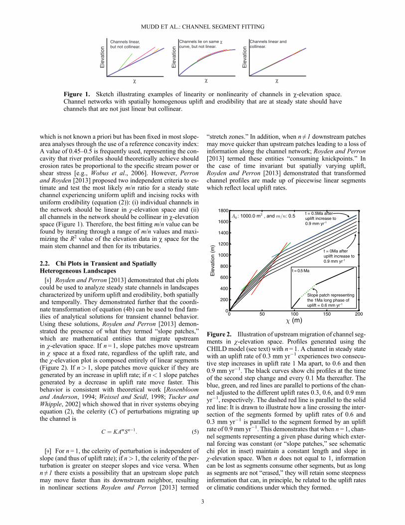
[8] Royden and Perron [2013] demonstrated that chi plotscould be used to analyze steady state channels in landscapescharacterized by uniform uplift and erodibility, both spatiallyand temporally. They demonstrated further that the coordi-nate transformation of equation (4b) can be used to find fam-ilies of analytical solutions for transient channel behavior.Using these solutions, Royden and Perron [2013] demon-strated the presence of what they termed “slope patches,”which are mathematical entities that migrate upstreamin χ-elevation space. If n= 1, slope patches move upstreamin χ space at a fixed rate, regardless of the uplift rate, andthe χ-elevation plot is composed entirely of linear segments(Figure 2). If n> 1, slope patches move quicker if they aregenerated by an increase in uplift rate; if n< 1 slope patchesgenerated by a decrease in uplift rate move faster. Thisbehavior is consistent with theoretical work [Rosenbloomand Anderson, 1994; Weissel and Seidl, 1998; Tucker andWhipple, 2002] which showed that in river systems obeyingequation (2), the celerity (C) of perturbations migrating upthe channel is

C ¼ KAmSn�1: (5)

[9] For n = 1, the celerity of perturbation is independent ofslope (and thus of uplift rate); if n> 1, the celerity of the per-turbation is greater on steeper slopes and vice versa. Whenn ≠ 1 there exists a possibility that an upstream slope patchmay move faster than its downstream neighbor, resultingin nonlinear sections Royden and Perron [2013] termed

“stretch zones.” In addition, when n ≠ 1 downstream patchesmay move quicker than upstream patches leading to a loss ofinformation along the channel network; Royden and Perron[2013] termed these entities “consuming knickpoints.” Inthe case of time invariant but spatially varying uplift,Royden and Perron [2013] demonstrated that transformedchannel profiles are made up of piecewise linear segmentswhich reflect local uplift rates.

χ

Ele

vatio

n

χ

Ele

vatio

n

χ

Ele

vatio

n

Channels linear,but not collinear.

Channels lie on same χ curve, but not linear.

Channels linear andcollinear.

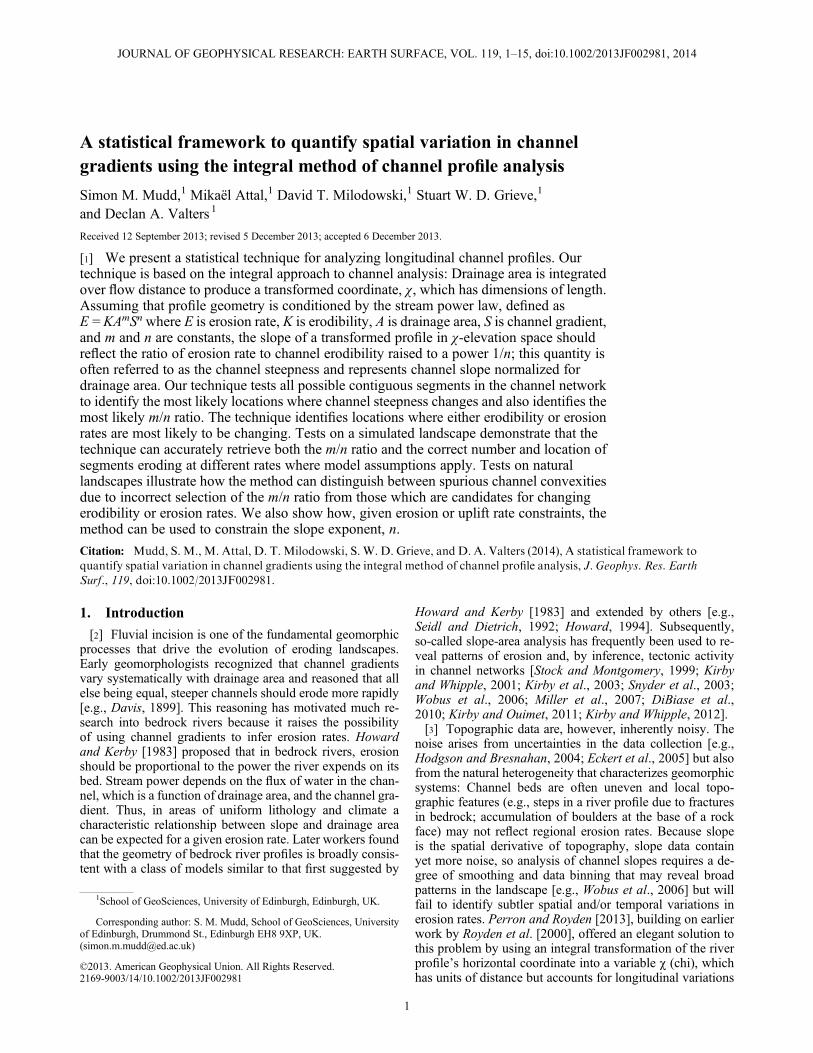
Figure 1. Sketch illustrating examples of linearity or nonlinearity of channels in χ-elevation space.Channel networks with spatially homogenous uplift and erodibility that are at steady state should havechannels that are not just linear but collinear.

0 50 100 150 2000

200

400

600

800

1000

1200

1400

1600

1800E

leva

tion

(m)

t = 0.5 Ma

Slope patch representing the 1Ma long phase of uplift = 0.6 mm yr

t = 0.5Ma after uplift increase to 0.9 mm yr

t = 0Ma after uplift increase to 0.9 mm yr

Figure 2. Illustration of upstreammigration of channel seg-ments in χ-elevation space. Profiles generated using theCHILD model (see text) with n = 1. A channel in steady statewith an uplift rate of 0.3 mm yr�1 experiences two consecu-tive step increases in uplift rate 1 Ma apart, to 0.6 and then0.9 mm yr�1. The black curves show chi profiles at the timeof the second step change and every 0.1 Ma thereafter. Theblue, green, and red lines are parallel to portions of the chan-nel adjusted to the different uplift rates 0.3, 0.6, and 0.9 mmyr�1, respectively. The dashed red line is parallel to the solidred line: It is drawn to illustrate how a line crossing the inter-section of the segments formed by uplift rates of 0.6 and0.3 mm yr�1 is parallel to the segment formed by an upliftrate of 0.9 mm yr�1. This demonstrates that when n = 1, chan-nel segments representing a given phase during which exter-nal forcing was constant (or “slope patches,” see schematicchi plot in inset) maintain a constant length and slope inχ-elevation space. When n does not equal to 1, informationcan be lost as segments consume other segments, but as longas segments are not “erased,” they will retain some steepnessinformation that can, in principle, be related to the uplift ratesor climatic conditions under which they formed.

MUDD ET AL.: CHANNEL SEGMENT FITTING

3

2.3. Need for a Statistical Approach to Create Chi PlotsFrom Topographic Data

[10] To construct chi plots, the m/n ratio must be assigned.Perron and Royden [2013] suggest performing linear regres-sion for a range of m/n ratios and selecting the ratio with theminimum value of R2. However, as discussed in the previoussection, the results of Royden and Perron [2013] imply that,in transient landscapes, spatial or temporal changes in upliftrates could lead to channel profiles that are piecewise linear.This hinders attempts to find the most likelym/n value. For ex-ample, a channel that has undergone stepwise increases in up-lift rates will be composed of two or more segments and willthus appear convex up (with a low R2 value) in the chi plot withthe true m/n ratio (Figure 3). Perron and Royden [2013] alsosuggested that in simple transient cases the collinearity of trib-utaries can be used to identify the correct m/n ratio, highlight-ing the need for statistical tests that go beyond minimizationof an R2 value. Thus, if our aim is to identify slope patches thatare indicative of spatial or temporal changes in boundary con-ditions (uplift or climate) or rock properties, we need an objec-tive, statistically robust, and reproducible method for doing so.In this contribution we present one such method.

3. A Statistical Method to Identify the Most LikelyCombination of Segments in χ- Elevation Space

[11] The method begins with a channel network for whichelevation (z), flow distance (x), and drainage area (A) havebeen extracted. Our approach tests every possible combina-tion of linear channel segments to find the most likelym/n ra-tio and the most likely piecewise linear fit to channel profiledata in χ-elevation space.

3.1. Integration of the Channel Profile

[12] The first step is to calculate the χ coordinate by integrat-ing equation (4b) for each node in the channel network. For in-tegration, we use the rectangle rule because increases in drainagearea are focused at tributary junctions; the rectangle rule bettercaptures the stepped nature of changes in drainage area alongchannels than other methods such as the trapezoid rule.

3.2. Segment Fitting Algorithm

[13] Our method relies on an algorithm that separates datainto the most likely combination of piecewise linear segments.

We favor a technique that uses piecewise fitting over other ap-proaches such as spline fitting [e.g., Hansen and Kooperberg,2002], which joins segments that share end nodes, otherwisecalled “knots.” We do not tie segments because we want atechnique that can capture the two types of knickpoints de-scribed by Kirby and Whipple [2012] as “vertical step”knickpoints, where there is a step between adjacent nodes inthe channel network, as well as those they describe as “slopebreak” knickpoints where channel steepness differs aboveand below the knickpoint.3.2.1. Partitioning the Data[14] The first step in the segment fitting algorithm is to “par-

tition” the data. Partitioning involves finding every combinationof positive integers that sum to some integer N (e.g., 5 can bepartitioned as 5; 4+1; 3+ 2; and 3+1+1). In our application,N is the number of nodes in χ-elevation space that we use fora particular channel, channel segment, or channel network.We use the partitioning algorithm described in Skiena [1990]and implemented by Frank Ruskey (http://theory.cs.uvic.ca/inf/nump/NumPartition.html). To allow the user to define aminimum number of nodes in a segment, we have modifiedthe Skiena [1990] algorithm to reject partitions that have lessthan the minimum number of nodes. The user is allowed to se-lect a minimum number of nodes in a segment because we rea-son that allowing segments made up of two nodes, while alwaysresulting in a perfect fit, will not be useful in reconstructingchannel dynamics. We explore the sensitivity of results tothe minimum segment length in sections 4.1 and 4.3.[15] The partition function, often denoted by P(N), describes

how many partitions there are for a given integer N. This func-tion is highly nonlinear. Example values of P(N) are P(10) = 42;P(100) = 190,569,292; P(200) = 397,299,029,388 [Andrews,1998]. The nonlinearity of the partition function precludesanalysis of more than a few hundred nodes due to computa-tional expense. We address this impediment to sampling everynode in the network by using a Monte-Carlo samplingapproach; each iteration samples a subset of nodes at reducedcomputational expense. This procedure is repeated until allnodes are sampled multiple times (section 3.2.2).[16] Partitioning alone does not sample all possible channel

segments, because segments could be arranged in different or-ders. Consider a channel with five nodes, further constrainedby a minimum segment length of two; the possible partitionsare therefore 5 and 3+ 2; however, the possible segment

= 0.99213

= 0.3

= 0.95290

= 0.5

max

imum

at

a. b. c.

= 0

.3Figure 3. (a) Plot shows the R2 values of a linear fit to channel data generated by the transient simulationdescribed in Figure 2 as a function of the m/n ratio. (b) Plot shows the profile in χ-elevation space with anm/n ratio of 0.3, which has the highest R2 for a linear fit to the channel data. (c) The true m/n is 0.5, and theχ- elevation profile for this m/n ratio is shown.

MUDD ET AL.: CHANNEL SEGMENT FITTING

4

combinations are 5, 3 + 2, and 2 + 3. We therefore permute allpartitions to sample all possible segment combinations.[17] A linear regression is performed on each segment. The

slope, intercept, residuals, and R2 of each segment are stored.Royden and Perron [2013] showed that under certain condi-tions (e.g., transience caused by changes in uplift rate withn ≠ 1), linear segments of the channel profile in the chi plotwill be connected by nonlinear segments (or “stretch zones”).Rather than performing both a linear and nonlinear fit on ev-ery segment, we perform only a linear fit. The rationale forthis is that (i) we do not wish to overconstrain the fit, (ii)selecting the incorrect m/n ratio results in nonlinear sectionsin χ-elevation space, and we do not wish to “reward”nonlinearity as this could lead to poor constraints on them/n ratio, and (iii) there is a simple relationship betweenthe linear segments’ slope and erosion rate in χ-elevationspace which does not apply in the stretch zones [seeRoyden and Perron, 2013, equation (16)].[18] As the number of nodes in the channel grows, there is

an ever increasing likelihood that some segments will besampled more than once. For example, consider a channelwith nine nodes and a minimum segment length of three.The partitions would then be 9; 6 + 3; 5 + 4; and 3 + 3 + 3.The segment starting on the first node and ending on the thirdnode will be used in the partition 3 + 6 as well as the partition3 + 3 + 3. To reduce computational expense, we precedepartitioning by regressing all segments and storing the slope,intercept, R2, and a maximum likelihood estimator (MLE) ofthe regressed χ-elevation data in sparse matrices where therow represents the starting node of the segment and the col-umn represents the finishing node of the segment.3.2.2. Determining the Most Likely Combinationof Segments[19] The partition algorithm finds every possible combina-

tion of segment lengths, and permuting through these segmentlengths results in every possible combination of segmentsalong a thinned channel network. Because the partition func-tion is highly nonlinear, it is necessary to limit the number ofnodes considered by the segment fitting algorithm. The algo-rithm allows the user to select the maximum number of nodesto be analyzed in any given iteration of the segment fitting al-gorithm. Whereas partitioning 100 nodes requires 109 linearregressions, partitioning 200 nodes requires ~1012 regressions.Beyond 200 nodes the computational expense is prohibitive;we recommend setting the maximum number of nodes (or“target nodes”) to 80–150. This creates a problem of resolutionhowever because, in high-resolution data, channels may bemade of more than 150 nodes; furthermore, we want to avoida situation in which the resolution of the analysis depends onthe number of nodes in the channels. We address this throughan iterative approach which, for computational efficiency,samples a subset of data in each iteration but through iterationssamples every data point in the channel network.[20] We use what we call a “skipping” algorithm to select a

subset of nodes from a data set. First, the number of nodes inthe data set is compared to the target nodes to determine themean number of nodes that must be “skipped” between twoselected nodes to retain the correct number of target nodesin the thinned data set. For example, if the data set has 300nodes and target nodes = 100, then for every node retained,the algorithm will skip two nodes. Skipping of data, how-ever, is done probabilistically, although the first and last

nodes are always selected. After a node is selected, the codeselects the next number of nodes to skip from a uniform dis-tribution centered on the mean skip value with a range twicethe mean skip value; for example, if the mean skip value is 2,skip values will be chosen in the range 0 to 4.[21] The skip interval is determined by the number of nodes

in the data set, but the user selects a “target skip” value whichis the final resolution of the data at which the user wants to per-form the analysis. Our iterative approach breaks the data setinto smaller and smaller pieces until the mean skip (deter-mined by dividing the number of data nodes by the numberof target nodes) matches that of the target skip value.[22] To iterate to the target skip value, all the data are

thinned using the probabilistic skipping algorithm, and thesedata are then passed to the segment fitting algorithm. Thefitting algorithm then determines the most likely segmentsfor the data and returns the segment number associated witheach node (Figure 4). This is recorded for each node in theanalysis, and the process is repeated. Because the skippingalgorithm is probabilistic, a different subset of nodes is ana-lyzed in each iteration. After many iterations, each node willbe associated with a data set comprising the number of thesegment to which it will have been attributed in each iteration(Figure 4). The mean of these numbers is then calculated foreach node. For nodes that lie unambiguously in a particularsegment (for example, the first node is always in the first seg-ment), the mean segment number will be an integer. Betweenunambiguous segments lie noninteger mean segment num-bers. If the mean skip is greater than the target skip, the dataare “broken” at natural segment breaks at nodes nearest tohalf an integer value (i.e., 1.5, 2.5, and 3.5). After breakingthe data, each smaller data set is passed back to the segmentfitting algorithm. This process is repeated until all of the“breaks” are analyzed at the resolution determined by theuser-defined target skip value.[23] Because a probabilistic approach is used to select data

nodes repeatedly, each node records the slope and interceptof the segments in χ-elevation space, as well as the segmentnumber and R2 value. The mean and standard deviation ofthese data for each node is then calculated. Of these, the slopein χ-elevation space, which we call Mχ, is perhaps the mostuseful because it is related to the ratio between erosion rate(E) and erodibility (K):

M χ ¼ E

KA0m

� �1=n

: (6)

[24] The intercept in χ-elevation space, which we call Bχ,can be used to identify steps in the channel network (e.g.,segments that have the same Mχ but are separated by a verti-cal waterfall). Thus, by constraining both Mχ and Bχ we areable to identify two types of knickpoints: a change in Bχ withno change in Mχ above and below the knickpoint indicates avertical step knickpoint, whereas a change in Mχ reveals aslope break knickpoint.[25] The next step is to calculate anMLE for each segment:

MLE ¼ ∏N

i¼1

1ffiffiffiffiffi2π

pσexp � rið Þ2

2σ2

" #; (7)

where σ [L] is the standard deviation of the measuredelevations. Many topographic data sets contain metadata

MUDD ET AL.: CHANNEL SEGMENT FITTING

5

describing the uncertainty of the elevations, which can guidethe choice of σ. However, we also suggest considering“geomorphic noise,” that is, variation in the channel profiledue to heterogeneity on scales of meters to tens of meters

(i.e., fracture patterns in rocks, bedrock sedimentary bedding,and boulders in the channel) that adds roughness to the chan-nel profile and clouds the landscape-scale geometry of theriver profile which is indicative of regional tectonics, lithol-ogy, or climate. The choice of σ will therefore depend onthe application, and it is therefore crucial that users of thesoftware report the value of this parameter. In section 4.1we report on how much of an impact changing the value ofσ can have on the number of segments selected by the soft-ware. Note that the MLE is multiplicative so that its valuefor a sequence of segments will be the product of the MLEof the individual segments.[26] For a fixed number of segments, the most likely

combination of these segments simply has the lowest MLEvalue. However, increasing the number of segments alwaysresults in a higher likelihood. Using the MLE alone is thusinsufficient to differentiate models with different numbersof segments.[27] An established statistical method for selecting a model

that balances goodness of fit against model complexity is theAkaike Information Criterion (AIC) [Akaike, 1974]:

AIC ¼ 2k � 2 ln MLEð Þ; (8)

where k is the number of parameters. Each linear segment hastwo parameters, the slope of the line and its intercept, sok = 2s where s is the number of segments. The model withthe minimum value of the AIC is deemed the best model.Burnham and Anderson [2002] suggest that a correctionshould be made to the AIC if there are a finite number of sam-ples; we therefore employ a corrected AICc [Hurvich andTsai, 1989] to select the best model:

AICc ¼ AICþ 2k k þ 1ð ÞN � k � 1

; (9)

where N is the sample size, or in this case the number ofchannel nodes used in the analysis. The AICc penalizes overfitting in small data sets, and Burnham and Anderson [2002,p. 445] suggest using AICc when N/k< 40. Because of therestriction on the number of nodes due to the computationalexpense of partitioning, almost any fitting of χ-elevation datawill meet this criterion, and AIC converges to AICc whenN is large so in the rare instances when the criterion fails(i.e., N/k> 40) AICc and AIC will take similar values.Thus, there is little reason to risk biasing the result by usingthe AIC rather than AICc. Figure 5 illustrates this partitioningprocess. We do not penalize segments whose fitted down-stream node is lower than the elevation of the fitted upstreamnode; this is because if sections are connected by stretchzones, a linear fit to a nonlinear stretch zone can result in seg-ments that do not always exhibit end nodes of monotonicallyincreasing elevations.[28] The choice of standard deviation (σ) in equation (7)

will affect the output of the fitting algorithm. For a fixednumber of segments, the most likely segments will alwaysbe the same, regardless of the value of σ. That is, the numericvalue of the MLE will change but the most likely combina-tion will not. Modifying the numeric value of the MLE, how-ever, changes the second term of equation (8) but does notaffect the first term of this equation. The result is that greater

node

7no

de 7

node

12

node

12

node

17

node

17

node

21

node

21

node

21

node

27

node

27

node

30

node

30

node

30

Ele

vatio

n

Raw Data

Ele

vatio

nE

leva

tion

Ele

vatio

n

a.

Node number (with equally spaced χ) 0 5 10 15 20 25 30

b.

c.

Node number (with equally spaced χ) 0 5 10 15 20 25 30

d.

Node number (with equally spaced χ) 0 5 10 15 20 25 30

Node number (with equally spaced χ) 0 5 10 15 20 25 30

Figure 4. Cartoon depicting the skipping process and theselection of segment numbers. (a) A hypothetical data setwith 31 data points is shown. (b–d) Plots show data afterskipping. In this case the mean skip = 1, so skip values arerandomly selected between 0, 1, and 2. In this hypotheticalexample, there are three iterations of the skipping algorithm.We highlight several nodes with yellow dots. Node 0 andnode 7 are always in the first segment, so the mean segmentnumber of these nodes will be = 1. The mean segment num-ber of node 12 will be 1.5 since it is in segment 1 in the firstiteration and segment 2 in the second iteration. Node 17 hasan integer mean segment number, whereas nodes 21, 27,and 30 all have noninteger mean segment numbers.

MUDD ET AL.: CHANNEL SEGMENT FITTING

6

values of σ result in greater “penalties” for extra segmentsand in general the lower the value of σ, the more segmentswill be selected.

3.3. Selection of the m/n Ratio

[29] To differentiate between profiles generated using dif-ferent m/n ratios, we use the MLE and AICc information.Again, the MLE is not sufficient to discriminate fitted chan-nel segments against each other because different m/n ratiosmay generate different numbers of best fit segments. Wetherefore store the cumulative AICc values for allm/n values.The m/n ratio that produces the minimum cumulative AICcvalue is considered the most likely. We perform two teststo determine the most likely m/n ratio: a collinearity testand a test for individual channels.[30] In the collinearity test, the data from the entire channel

network are pooled. This pooled data set undergoes thebreaking processes described in section 3.2.2, but the AICcvalues reported are cumulative for all the data rather thanon a channel by channel basis. Our testing based on numeri-cal simulations (see section 4.1) indicates this test can betteridentify the m/n ratio when analyzing data based on numeri-cal simulations. Our tests on channels in natural environ-ments (e.g., section 4.2) indicate however that there can bepitfalls to this method. If a tributary is hanging, for example,the data from this tributary will be lying above the main

stem’s data in χ-elevation space (by definition); because thealgorithm will seek them/n value that best superimposes datafrom the tributary and the main stem, the collinearity test maygive spurious results for the best fit m/n ratio.[31] The second test calculates the cumulative value of the

AICc for each individual channel. In this analysis, all tribu-taries are extended from their source to the drainage outlet.The rationale for this is that transient signals of uplift rateare translated through the channel network with celerity pro-portional to drainage area (see equation (5)) [Whipple andTucker, 1999]. This means that any upstream propagationof uplift signals will slow down significantly as it enterssmall tributaries: steepened reaches in small tributaries willconsequently often have limited spatial extent. The result isthat if tributary channels are extended only to the junctionwith the main stem, the algorithm will not be able to findthe short transient segment. The segment can be found, how-ever, if the analyzed channel data include the tributary dataand the main stem data downstream of the confluence.[32] As described in section 3.2.2, the mean AICc values are

a result of many iterations of the segment fitting algorithm.The code also returns the standard deviation of the AICcvalues for each m/n ratio, for the cumulative data (used inthe collinearity test), and for each individual channel. The var-iability is due to the algorithm being performed on a differentsubset of data, chosen at random by the skipping algorithm,

Figure 5. Illustration of the partitioning process (minimum partition length = five nodes in this case).

MUDD ET AL.: CHANNEL SEGMENT FITTING

7

during individual iterations. The most likely m/n ratio is thatwith the minimum AICc value, but the standard deviation ofthe AICc values can be used to infer the range of plausiblem/n values for the channel network. We recommend that au-thors interpret the m/n ratios with AICc values that are within1 standard deviation of the minimum AICc values as being“plausible.” Figure 6 shows a flowchart of the segment fittingalgorithm. We have made the code available at theCommunity Surface Dynamics Modeling System website:http://csdms.colorado.edu/wiki/Model:Chi_analysis_tools.

4. Examples

[33] We illustrate the technique using three examples. Thefirst example uses topography generated from the Channel-Hillslope Integrated Landscape Development (CHILD)model [Tucker et al., 2001]. This allows us to test whetherthe technique can identify known segments and retrieve aknown m/n ratio. The next two examples are from naturallandscapes. The first is from the Appalachian Plateau inPennsylvania, U.S., where the combination of relativelyhomogenous sandstone bedrock and tectonic quiescence isthought to result in steadily eroding channels [Hack, 1960].

The second is from a landscape in the Apennines in Italy thathas been subject to a previously constrained change in tec-tonic uplift rate [e.g., Whittaker et al., 2008].

4.1. A Numerical Example: A Simulated Three-StageAcceleration in Uplift

[34] Our first example deploys our chi analysis method ona landscape simulated with the CHILD landscape evolutionmodel. We have chosen to run the method on a numericalsimulation because it allows us to enforce equation (1) andto prescribe both the uplift history and m/n ratio. Our simula-tion involves three development stages. The model domain isa 6 × 6 km2 with an average node spacing of 50 m.Throughout the simulation, one boundary is set to a fixed el-evation (defined as z= 0 m), and the other boundaries are noflux boundaries. We use model parameters adapted fromAttal et al.’s [2011] study of the evolution of catchmentsresponding to tectonics in the Apennines using the CHILDmodel. Erosion is purely detachment limited: Erosion ratesare calculated according to equation (1); furthermore, there isneither threshold for erosion nor adjustment in channel geom-etry [Attal et al., 2011]. The parameters used in the model andthe calculation of erosion rates are detailed in the Appendix A.The hillslope transport coefficient is set to 0.001 m2 yr�1,channel erodibility (K) is set to 1.67 × 10�6 yr�1, m is set to0.5 and n is set to 1 (Appendix A). In the first stage, a fixeduniform uplift rate of 0.3 mm yr�1 is prescribed. This upliftrate is maintained until the model domain achieves dynamicsteady state, that is, erosion rates match the uplift rate of0.3 mm yr�1 throughout the entire landscape. At this stage,rivers are characterized by smooth concave up river profiles.The uplift rate is then increased to 0.6 mm yr�1 for 1 Ma andthen further increased to 0.9 mm yr�1 for a further 0.5 Ma. Inresponse to the successive increases in uplift rate, steepenedreaches develop upstream of the base level, separated fromthe upstream reaches by profile convexities that migrateupstream through time, representing the propagation of ero-sional waves that is diagnostic of detachment-limited systems[e.g., Whipple and Tucker, 1999; Attal et al., 2011].[35] The CHILD model runs on a triangulated irregular

network (TIN), and channel profiles are extracted directlyfrom the TIN. We use equation (1) to calculate erosion ratesalong the channels at the end of the run and find threesections with distinct erosion rates separated by transitionzones (Figure 7a). We infer that these transition zones arepresent because CHILD uses an explicit numerical method(i.e., it uses model topographic parameters to calculatetopographic changes at the following time step; Tuckeret al. [2001]), which is susceptible to numerical dispersion[e.g., Fagherazzi et al., 2002]. At the end of our simulation,the main stem river profile features two prominent convexi-ties delineating three reaches (Figure 7b): upstream of the up-permost convexity, the river profile is adjusted to the initialuplift rate of 0.3 mm yr�1 and has not responded to any ofthe increases in uplift rate; between the two convexities, theriver profile has adjusted to the uplift rate of 0.6 mm yr�1;downstream of the lowermost convexity, the steep reach isin equilibrium with the final uplift rate of 0.9 mm yr�1. Thetwo convexities are migrating upstream in concert at a celer-ity given by equation (5). Because n = 1 in the model, the ce-lerity is independent of slope and thus of uplift rate so theconvexities never meet, and the intermediate segment is

Figure 6. Flowchart for the segment fitting algorithm.

MUDD ET AL.: CHANNEL SEGMENT FITTING

8

preserved until the wave of erosion has propagated all theway to the top of the network.[36] Results from segment extraction with the best fit m/n

ratio of 0.5 (see next paragraph) demonstrate that the algorithmis able to detect the sections of the channel network respondingto different uplift rates (Figures 7b–7d). In addition to beingable to identify distinct channel segments, the algorithm is alsoable to retrieve Mχ values extremely close to the theoreticalvalues predicted by equation (6) (Figure 7c).[37] Our segment fitting algorithm is able to tightly con-

strain the most likely m/n ratio for these simulations.Figures 8a and 8b show that plausible values of the m/n ratio(those that have AICc values within 1 standard deviation ofthe m/n ratio with the minimum AICc value) clustered tightlyaround 0.5 (in Figures 8a and 8b, m/n ratios of 0.475–0.525are considered plausible). The method correctly identifiesthe m/n ratio of 0.5 as the most likely.4.1.1. Sensitivity Analysis and RecommendedDefault Parameters[38] We performed a sensitivity analysis on the effect of

changing the number of target nodes, the minimum segmentlength, the value of σ and the mean skip value using resultsfrom the CHILD simulations. We varied σ from 1 to 9 m,the mean skip value from 1 to 4, the minimum segmentlength from 6 to 20 nodes, and the number of target nodesfrom 60 to 100. Parameters generated similar results over awide range of values for the main stem. The minimum

segment length and number of target nodes, however, can sig-nificantly alter computational time. Running the method onthe CHILD data with target nodes = 100 and minimum seg-ment length= 20 took a few minutes, whereas the run with tar-get nodes = 100 and minimum segment length= 5 took 4 dayson our Linux servers (i.e., 5–6 orders of magnitude longer).This strong dependence on computation time is due to thenonlinearity of the partition function. Sensitivity analysisshows that (i) increasing σ, the minimum segment length orthe mean skip decreases the number of segments; (ii) one con-sequence of reducing the number of segments is that tributarieswill be fit with single segment and information about changingsteepness will be lost; and (iii) the number of target nodes canhave a large influence on computational time but does not havea commensurate effect on the extracted segments. The leastconclusive results were obtained when high values of meanskip (≥ 3) or minimum segment length were used.[39] In every analysis performed by the method on the

CHILD model runs, the most likely m/n ratio has been calcu-lated as 0.5. The best fit m/n ratio has similarly retuned 0.5 asthe most likely m/n ratio for all individual channels except inthe cases where minimum segment length or mean skip pa-rameters have resulted in <3 segments, which only occurredin the shortest tributaries.[40] Our sensitivity analyses on the CHILD runs and in

other landscapes have helped us develop some qualitativerules of thumb for selecting parameter values. We suggest

Figure 7. Results from CHILD model runs. (a) Erosion rates calculated along the channel (b, c) denotedby a star using equation (1), which is prescribed in the model. Figure 7b denotes channel longitudinal pro-files colored by the extractedMχ values. Figure 7c showsMχ values as a function of χ; each tributary is de-noted by a different color. The tributary depicted in Figure 7a (star in Figure 7b) is plotted in black. (d) Chiplot of fitted and transformed data of all channels. In Figures 7a, 7c, and 7d the red- and green-shaded barsdenote the transition zones between domains adjusted to the different phases of uplift. The horizontal red,green, and blue lines in Figure 7c represent the Mχ values corresponding to erosion rates of 0.9 mm yr�1,0.6 mm yr�1, and 0.3 mm yr�1, respectively, calculated using equation (6). Figures 7b–7d were generatedwith a mean skip value of 1, a minimum segment length of 12, 100 target nodes, and a σ value of 3 m.

MUDD ET AL.: CHANNEL SEGMENT FITTING

9

minimum segment lengths of 10–15 and a number of targetnodes of 80–100. Increasing the number of target nodes doesnot seem to alter results substantially and results in very longcompute times. Standard deviation of elevations (σ) and theskip value should be selected based on the resolution andquality of the digital elevation model (DEM). For 30 to90 m resolution DEMs, we suggest skip values of 0–2 andσ values on the order of tens of meters. Ten meter resolutionDEMs should have skip values of 1 to 4 and a σ similar to thereported uncertainty in elevation data, with some additionaluncertainty due to topographic “noise” (i.e., boulders inchannels). For 1 to 2 m resolution data, skip values of 5–10will be more appropriate, and σ will most likely be on the or-der of meters. These parameters can be used to rapidly iden-tify segments in a channel network; however, naturalchannels are not all as well behaved as simulated channels(see section 4.3) so we suggest that a sensitivity analysis isconducted as part of any analysis of channel steepness.

4.2. Fonner Run in Southwest Pennsylvania, U.S.

[41] Our second example comes from the western flank ofthe Appalachians in southwest Pennsylvania. We have se-lected a small basin called Fonner Run at 39.969391°N,80.254147°W, for analysis (Figure 9a). This basin is in thesame tectonic and geologic setting as Rush Run, which wasanalyzed by Perron and Royden [2013], but lies ~140 km tothe northeast. Rivers here flow through a dendritic channelnetwork over sandstone bedrock [Miles and Whitfield, 2001].

The site is tectonically quiescent and is to the south of thesouthernmost extent of Quaternary glaciations [Peltier, 2004].[42] Our method finds a best fit m/n ratio of 0.675 based on

the collinearity test, whereas the best fit m/n ratio of the mainstem channel is 0.65 (Figures 8c and 8d). Plots of AICc as afunction of m/n ratio at this site indicate that plausible values(i.e., those within 1 standard deviation of the minimumAICc,in this case after 250 iterations of the segment finding algo-rithm) for the m/n ratio range from 0.6 to 0.7 (Figures 8cand 8d). For Rush Run, Perron and Royden [2013] foundthat, qualitatively, an m/n value of 0.65 best collapses thetributaries. They note that this m/n ratio leads to a convexup main stem channel. Our analysis of Fonner Run yieldsqualitatively the same result: the m/n ratio that best collapsesthe tributaries (as determined in our case by the collinearitytest) leads to a main stem that appears slightly convex(Figure 9). However, our segment fitting algorithm finds thatthe m/n ratio that best describes the main stem channel as aseries of linear segments is similar to the best fit m/n ratiofor collinearity. Because the two analyses yield similar re-sults, we can have some confidence that the main stem chan-nel does in fact have different segments, and the apparentconvexity is not simply a by-product of selecting an inappro-priate m/n ratio. Our segment fitting algorithm finds that thebest explanation for the channel profile is one made up oftwo segments, with the downstream segment having aslightly greater value of Mχ (Figure 9). This downstreamsteepening may have multiple causes, including changes in

a.

b.

c.

d.

Figure 8. Plot of AICc values as a function ofm/n ratio for CHILDmodel runs for (a) the main stem chan-nel and (b) the collinearity test, and for Fonner Run, PA, for (c) the main stem and (d) the collinearity test.Errors represent 1 standard deviation of the AICc value measured after 250 iterations of the segment findingalgorithm. Dashed line indicates the minimum AICc value plus 1 standard deviation. Red box shows rangeof m/n values where the AICc value is within 1 standard deviation of the minimum AICc value. Parametervalues are for CHILD runs, mean skip value = 1, minimum segment length = 12, number of target nodes =100, and σ= 3 m; for Fonner Run, mean skip value = 2, minimum segment length = 15, number of targetnodes = 100, and σ= 3 m.

MUDD ET AL.: CHANNEL SEGMENT FITTING

10

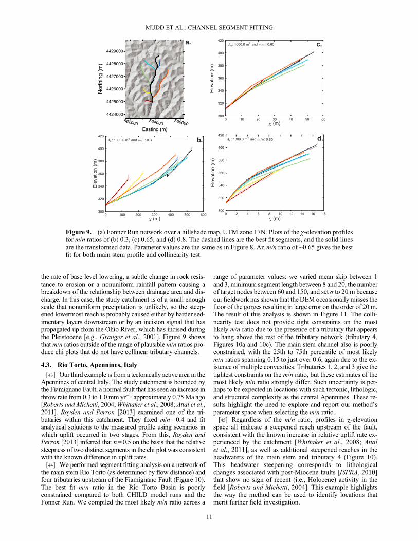
the rate of base level lowering, a subtle change in rock resis-tance to erosion or a nonuniform rainfall pattern causing abreakdown of the relationship between drainage area and dis-charge. In this case, the study catchment is of a small enoughscale that nonuniform precipitation is unlikely, so the steep-ened lowermost reach is probably caused either by harder sed-imentary layers downstream or by an incision signal that haspropagated up from the Ohio River, which has incised duringthe Pleistocene [e.g., Granger et al., 2001]. Figure 9 showsthat m/n ratios outside of the range of plausible m/n ratios pro-duce chi plots that do not have collinear tributary channels.

4.3. Rio Torto, Apennines, Italy

[43] Our third example is from a tectonically active area in theApennines of central Italy. The study catchment is bounded bythe Fiamignano Fault, a normal fault that has seen an increase inthrow rate from 0.3 to 1.0 mm yr�1 approximately 0.75Ma ago[Roberts and Michetti, 2004;Whittaker et al., 2008; Attal et al.,2011]. Royden and Perron [2013] examined one of the tri-butaries within this catchment. They fixed m/n=0.4 and fitanalytical solutions to the measured profile using scenarios inwhich uplift occurred in two stages. From this, Royden andPerron [2013] inferred that n=0.5 on the basis that the relativesteepness of two distinct segments in the chi plot was consistentwith the known difference in uplift rates.[44] We performed segment fitting analysis on a network of

the main stem Rio Torto (as determined by flow distance) andfour tributaries upstream of the Fiamignano Fault (Figure 10).The best fit m/n ratio in the Rio Torto Basin is poorlyconstrained compared to both CHILD model runs and theFonner Run. We compiled the most likely m/n ratio across a

range of parameter values: we varied mean skip between 1and 3, minimum segment length between 8 and 20, the numberof target nodes between 60 and 150, and set σ to 20 m becauseour fieldwork has shown that the DEMoccasionallymisses thefloor of the gorges resulting in large error on the order of 20 m.The result of this analysis is shown in Figure 11. The colli-nearity test does not provide tight constraints on the mostlikely m/n ratio due to the presence of a tributary that appearsto hang above the rest of the tributary network (tributary 4,Figures 10a and 10c). The main stem channel also is poorlyconstrained, with the 25th to 75th percentile of most likelym/n ratios spanning 0.15 to just over 0.6, again due to the ex-istence of multiple convexities. Tributaries 1, 2, and 3 give thetightest constraints on the m/n ratio, but these estimates of themost likely m/n ratio strongly differ. Such uncertainty is per-haps to be expected in locations with such tectonic, lithologic,and structural complexity as the central Apennines. These re-sults highlight the need to explore and report our method’sparameter space when selecting the m/n ratio.[45] Regardless of the m/n ratio, profiles in χ-elevation

space all indicate a steepened reach upstream of the fault,consistent with the known increase in relative uplift rate ex-perienced by the catchment [Whittaker et al., 2008; Attalet al., 2011], as well as additional steepened reaches in theheadwaters of the main stem and tributary 4 (Figure 10).This headwater steepening corresponds to lithologicalchanges associated with post-Miocene faults [ISPRA, 2010]that show no sign of recent (i.e., Holocene) activity in thefield [Roberts and Michetti, 2004]. This example highlightsthe way the method can be used to identify locations thatmerit further field investigation.

b.

c.

d.

562000564000

566000Easting (m)

4424000

4425000

4426000

4427000

4428000

4429000

Nor

thin

g (m

)

a.

Figure 9. (a) Fonner Run network over a hillshade map, UTM zone 17N. Plots of the χ-elevation profilesfor m/n ratios of (b) 0.3, (c) 0.65, and (d) 0.8. The dashed lines are the best fit segments, and the solid linesare the transformed data. Parameter values are the same as in Figure 8. An m/n ratio of ~0.65 gives the bestfit for both main stem profile and collinearity test.

MUDD ET AL.: CHANNEL SEGMENT FITTING

11

4.3.1. Using Mχ to Constrain the n Exponentin Locations With Known Uplift Rates[46] Royden and Perron [2013] asserted that in rivers with

similar precipitation and erodibility but different uplift rates,the ratio between Mχ values is proportional to the ratio be-tween uplift rates raised to the 1/n power. Here we explorethis assertion, which can be used to determine the n exponent,and extend it to cases where erodibility is a function of upliftrate, as suggested by some authors [e.g., Snyder et al., 2003].In segments unaffected by stretch zones,Mχ is related to ero-sion rate, erodibility and other parameters according to equa-tion (6). Assuming that segments represent stretches of theriver equilibrated to the uplift rate that led to their formation,uplift rate can be substituted for erosion rate, and equation (6)can be rearranged as follows:

M χnKA0

m ¼ U : (10)

[47] If we have two separate segments with separate valuesof Mχ we can relate these to a ratio between uplift rates:

M χ;1nKA0

m

M χ;2nKA0

m ¼ U1

U2: (11)

[48] Again, this equation assumes that there has been someequilibration between uplift and erosion rate or, in otherwords, that uplift has been sustained for long enough to be

Figure 11. Box-and-whisker plot of the best fitm/n ratio forthe Rio Torto channel network. The red lines are the medianmost likely m/n ratios across 30 parameter values (varyingskip, minimum segment length, and number of target nodes).The whiskers are the data range (with one outlier in channel3), the boxes extend between the 25th and 75th percentilesof the data, the tapering extends to the 95% confidence inter-vals of the median most likely m/n ratio calculated bybootstrapping the data 10,000 times. Dashed lines insertedas a visual aid to identify m/n ratios of 0.5, 0.6, and 0.7.

Figure 10. Results of segment fitting algorithm for the Rio Torto and tributaries using anm/n ratio of 0.6.Parameter values are mean skip = 1, number of target nodes = 100, minimum segment length = 12, andσ= 20 m. (a) Channel profiles colored by the best fit Mχ. (b) Calculated values of Mχ for each tributary.Dashed gray lines denote segments selected to calculate Mχ ratio. (c) Best fit segments (dashed lines)and transformed data (solid lines) in χ-elevation space. (d) Map of Rio Torto projected in UTM zone33N; the outlet of the study catchment is at approximately 42.267655°W, 13.186485°E. Channels coloredby best fit Mχ shown on a hillshade of the study catchment.

MUDD ET AL.: CHANNEL SEGMENT FITTING

12

reflected in the channel profile. Therefore, estimates of ero-sion rates or uplift rates that represent timescales of thou-sands to millions of years would be appropriate for such ananalysis, whereas measurements of suspended sediment,which vary on interannual timescales, may not capture thefull range of erosion rates that drive topographic signaturesof uplift rates. The parameter A0 is a constant, and if we as-sume K is a constant, equation (11) simplifies to

M χ;1

M χ;2

� �n

¼ U 1

U 2: (12)

[49] The ratio of uplifts is thus equal to the ratio of Mχ tothe power n.[50] Some authors have suggested that the erodibility of

bedrock channels is a function of uplift rates. If we assumethe erodibility coefficient has the form K= kUa [e.g., Snyderet al., 2003; DiBiase et al., 2010], then equation (12) canbe recast as

M χ;1

M χ;2

� �ne

¼ U 1

U 2; (13)

where ne is an “effective” slope exponent where ne= n/(1� a).If we solve equation (12) for the slope exponent n (and notethat equation (13) has the same form as equation (12) so cansimilarly be solved for ne), we find that

n ¼ LogU1

U2

� �=Log

M χ;1

M χ;2

� �� �: (14)

[51] In practice, one can only use equation (14) if the m/nratio is constrained beforehand, since the m/n ratio affectsthe values ofMχ derived for each segment and thus theMχ ra-tio. In the Rio Torto, we follow Attal et al. [2011] and assumethe upstream segments are equilibrated to a fault throw rate of~0.3 mm yr�1 whereas the downstream segments are equili-brated to a fault throw rate of ~1.0 mm yr�1. These rates yieldan uplift ratio of ~3.3. Regardless of parameter combinations,the transformed channels are composed of several distinctsegments. We use the average value of Mχ from tributaries1, 2, and 3 to calculate Mχ ratios since these channels appearto have the most consistent profiles (Figures 10b and 10c).We use the most downstream segment on each of these chan-nels, which is bounded by the fault, and the segments in thesechannel that sit on the plateau.[52] Using these criteria leads to Mχ ratios of ~4.3, 8, and

10, respectively when the most likely m/n ratios are 0.5,0.6, and 0.7, respectively (Figure 11). These Mχ ratiosresult in an estimate of n between 0.52 and 0.82, that is,at the lower end of the range of values suggested basedon a physical description of the erosion processes at workin bedrock rivers [Whipple et al., 2000]. Note however thatin addition to the lithological variations mentioned insection 4.3, the complexity of the tectonic setting in theApennines may also lead to difficulties when trying to in-vert topographic data to retrieve stream power parameters:for example, the Rio Torto basin is experiencing back-tilting as it is being uplifted [e.g., Attal et al., 2011], poten-tially causing a reduction in the steepness of the upstream

reaches which may lead to an anomalously high Mχ ratio(and thus a low n estimate).

5. Conclusions

[53] We present a method for analyzing channel longitudi-nal profiles in order to extract information about erodibilityor erosion rates. Our method extracts the most statisticallylikely channel segments that have distinct steepness, normal-ized for drainage area through the integral method of channelprofile analysis. This method eliminates the need for initialprocessing of the raw topographic data (e.g., smoothing ofriver profiles to derive channel slope) which inevitably leadsto loss of information. In locations where the stream powerincision model can predict channel incision rates, our methodcan be used to quantify the most likely m/n ratio and locatechannel segments with distinct erosion rates or erodibilities(where erodibility refers to the K parameter in the streampower law, which encapsulates the influence of bedrockstrength, climate, sediment supply, erosion thresholds, andchannel width adjustment on the susceptibility of bedrockto fluvial erosion). The method also reports uncertainties inthe most likely m/n ratio. Our tests on an idealized, simulatedlandscape and on a landscape on the Appalachian Plateauresulted in tightly constrained m/n ratios and identificationof distinct segments within the fluvial networks. In the caseof the modeled landscape, these distinct segments predict-ably reflect the changes in uplift rate applied during the sim-ulation. In a tectonically and structurally complex landscapein the Apennines in Italy, the uncertainty on the estimates ofm/n ratio is much greater but the segments identified are nev-ertheless consistent with the known tectonic history of thearea. We also show how users may apply our method toquantify the n exponent in locations where erosion rates arewell constrained.

6. Author Contributions

[54] S.M.M. designed the algorithms. S.M.M., D.T.M., andS.W.D.G. wrote the code. M.A. performed CHILD simula-tions. S.M.M., D.T.M., S.W.D.G., and D.A.V. wrote vis-ualization scripts, and S.M.M., M.A., D.T.M., S.W.D.G.,and D.A.V. performed the analyses and wrote the paper.

7. Software Availability

[55] Source code, documentation, instructions, and chan-nel profile data are available via the Community SurfaceDynamics Modeling System at http://csdms.colorado.edu/wiki/Model:Chi_analysis_tools.

Appendix A: Description of the Calculationof Erosion Rates in the CHILD Model

[56] In the CHILD model, erosion rates are calculatedusing equations that can be combined to give equation (1)[see Tucker et al., 2001; Attal et al., 2011]. Simulationspresented here are for a scenario in which erosion is purely de-tachment limited, and there are neither erosion thresholds noradjustment in channel geometry [cf. Attal et al., 2008, 2011].First, the model calculates potential hillslope and fluvialerosion rates according to equations (A1) and (A2), respec-tively (see below). Erosion driven by soil creep is computed

MUDD ET AL.: CHANNEL SEGMENT FITTING

13

based on the divergence of volumetric sediment discharge perunit width qc, which is calculated with

qc ¼ �Kd∇z; (A1)

where Kd [L2 T�1] is a hillslope transport coefficient andz [L] is surface elevation. Fluvial erosion rate E [L T�1] iscalculated following:

E ¼ kbτ pb; (A2)

where kb is a specific bedrock erodibility coefficient (in L T�1

per “stress quantity” in SI units), τ [M L�1 T�2] is fluvialshear stress, and pb is a dimensionless constant. The erosionrate calculated by both equations is compared, and the elevationof the node is lowered by the largest amount predicted by eitherof the two equations. Beyond a given drainage area, fluvial pro-cesses become dominant, and equation (A2) prevails. The shearstress quantity (the unit of which depends on the values chosenfor exponents mb and nb) is calculated according to

τ ¼ kt Q=Wð ÞmbSnb; (A3)

whereQ is water discharge [L3 T�1,W [L] is channel width, ktis a scaling parameter, and mb and nb are constants. Here,channel width is calculated using the simplest form of hydrau-lic scaling available in CHILD [Leopold and Maddock, 1953]:

W ¼ kwQ1=2; (A4)

where kw is a hydraulic scaling coefficient [L�1/2 T1/2]. In themodel, we assume no infiltration so that discharge is only theproduct of the precipitation rate P in [L T�1] by drainagearea:

Q ¼ PA: (A5)

[57] Combining equations (A2) to (A5) gives

E ¼ kbktpb kw

�pb:mbð ÞP pb:mb=2ð ÞA pb:mb=2ð ÞS pb:nbð Þ: (A6)

[58] This equation is equivalent to equation (1), withm = pb.mb/2, n = pb.nb, and K= kb kt

pb kw(�pb.mb) P(pb.mb/2).

Note that the exponents mb, nb, and pb can be set to simulatedifferent fluvial incision laws (i.e., incision rate proportionalto fluvial shear stress, cross-section-averaged stream poweror specific stream power). In our example, we assume thaterosion rate is proportional to stream power per unit bed area(so-called specific stream power) and set mb = nb= pb= 1.Equation (A6) thus becomes

E ¼ KA1=2S (A7)

with K = kb kt kw�1 P1/2 [T�1]. We thus have m = 0.5, n = 1,

and m/n = 0.5. In this case, the quantity τ in equation (A3)represents the specific stream power [M T�3], and kt is thespecific weight of water (9810 kg m�2 s�2 in SI units).The value of kb has to be adjusted with respect to Attalet al.’s [2011] study where the exponents were set to differ-ent values (mb = 0.6, nb = 0.7, and pb = 1.5): in the presentstudy, we set kb = 2.2 × 10�5 m yr�1 (W m�2)�1 as theequivalent of the value of 5.2.10�6 m yr�1 Pa�3/2 that wasused in Attal et al. [2011]. We use kw = 4.6 m�1/2 s1/2 to

replicate the hydraulic scaling relationship without adjust-ment in channel geometry constrained in the Apennines[Attal et al., 2008]. We use rainfall parameters identical tothose in Attal et al. [2011], except that we do not allowthe parameters to vary around their mean value during theruns; the CHILD model produces storms according to aPoisson rectangular pulse rainfall model [Tucker andBras, 2000], using the following values: mean precipitationrate = 0.75 mm/h, mean storm duration = 22 h, and meaninterstorm duration = 260 h. This means that each year, itrains 7.8% of the time at a rate of 0.75 mm/h, thus equiva-lent to an average yearly rainfall P = 1.63 10�8 m s�1. Wethus derive K = 1.67 10�6 yr�1 (equation (A7)).

[59] Acknowledgments. We thank Jen Merritt, Fiona Clubb, AmyBall, Rahul Devrani, Vimal Singh, Martin Hurst, and T.C. Hales for betatesting the software. Greg Tucker provided advice on CHILD simulations,and we thank Taylor Perron, Sean Gallen, Alex Densmore, and an anony-mous referee for their comments and suggestions. This work was supportedby the Carnegie Trust for the Universities of Scotland and NERC grant NE/J012750/1 to Mudd. David Milodowski is supported by NERC grant NE/J500021/1, and Stuart Grieve is supported by NERC grant NE/J009970/1.

ReferencesAkaike, H. (1974), A new look at the statistical model identification, IEEETrans. Autom. Control, 19(6), 716–723, doi:10.1109/TAC.1974.1100705.

Andrews, G. E. (1998), The Theory of Partitions, England, Cambridge Univ.Press, Cambridge.

Attal, M., G. E. Tucker, A. C. Whittaker, P. A. Cowie, and G. P. Roberts(2008), Modeling fluvial incision and transient landscape evolution:Influence of dynamic channel adjustment, J. Geophys. Res., 113, F03013,doi:10.1029/2007JF000893.

Attal, M., P. A. Cowie, A. C. Whittaker, D. Hobley, G. E. Tucker, andG. P. Roberts (2011), Testing fluvial erosion models using the transient re-sponse of bedrock rivers to tectonic forcing in the Apennines, Italy,J. Geophys. Res., 116, F02005, doi:10.1029/2010JF001875.

Burnham, K. P., and D. R. Anderson (2002), Model Selection andMultimodel Inference: A Practical Information-Theoretic Approach, 2nded., 488 pp., Springer-Verlag, New York, ISBN:0-387-95364-7.

Cowie, P. A., A. C. Whittaker, M. Attal, G. P. Roberts, G. E. Tucker, andA. Ganas (2008), New constraints on sediment-flux-dependent river inci-sion: Implications for extracting tectonic signals from river profiles,Geology, 36, 535–538, doi:10.1130/G24681A.1.

Davis, W. M. (1899), The geographical cycle, Geogr. J., 14(5), 481–504.DiBiase, R. A., K. X. Whipple, A. M. Heimsath, and W. B. Ouimet (2010),Landscape form and millennial erosion rates in the San GabrielMountains, CA, Earth Planet. Sci. Lett., 289, 134–144, doi:10.1016/j.epsl.2009.10.036.

Eckert, S., T. Kellenberger, and K. Itten (2005), Accuracy assessment ofautomatically derived digital elevation models fromASTER data in moun-tainous terrain, Int. J. Remote Sens., 26(9), 1943–1957, doi:10.1080/0143116042000298306.

Fagherazzi, S., A. D. Howard, and P. L. Wiberg (2002), An implicit finitedifference method for drainage basin evolution, Water Resour. Res.,38(7), 116, doi:10.1029/2001WR000721.

Granger, D. E., D. Fabel, and A. N. Palmer (2001), Pliocene-Pleistocene in-cision of the Green River, Kentucky, determined from radioactive decay ofcosmogenic 26Al and 10Be in Mammoth Cave sediments, Geol. Soc. Am.Bull., 113(7), 825–836, doi:10.1130/0016-7606(2001)113%3C0825:PPIOTG%3E2.0.CO;2.

Hack, J. T. (1960), Interpretation of erosional topography in humid temper-ate regions, Am. J. Sci., 258-A, 80–97.

Hansen, M. H., and C. Kooperberg (2002), Spline adaptation in extendedlinear models, Stat. Sci., 17(1), 2–51, doi:10.1214/ss/1023798997.

Harkins N., E. Kirby, A. Heimsath, R. Robinson, and U. Reiser (2007),Transient fluvial incision in the headwaters of theYellowRiver, northeasternTibet, China, J. Geophys. Res., 112, F03S04, doi:10.1029/2006JF000570.

Hobley, D. E. J., H. D. Sinclair, S. M. Mudd, and P. A. Cowie (2011), Fieldcalibration of sediment flux dependent river incision, J. Geophys. Res.,116, F04017, doi: 10.1029/2010JF001935.

Hodgson, M. E., and P. Bresnahan (2004), Accuracy of airborne lidar-derived elevation: Empirical assessment and error budget, Photogramm.Eng. Remote Sens., 70(3), 331–339.

Howard, A. D. (1994), A detachment-limited model of drainage basin evolu-tion, Water Resour. Res., 30, 2261–2285.

MUDD ET AL.: CHANNEL SEGMENT FITTING

14

Howard, A. D., and G. Kerby (1983), Channel changes in badlands, Bull.Geol. Soc. Am., 94(6), 739–752.

Hurvich, C. M., and C.-L. Tsai (1989), Regression and time series modelselection in small samples, Biometrika, 76, 297–307.

ISPRA (2010), Carta geologica d’Italia, Foglia 658: Pescorocchiano(1:50,000), Servizio Geologico d’Italia.

Kirby, E., andW. Ouimet (2011), Tectonic geomorphology along the easternmargin of Tibet: Insights into the pattern and processes of active deforma-tion adjacent to the Sichuan Basin, Geol. Soc. Lond. Spec. Publ., 353,165–188, doi:10.1144/SP353.9.

Kirby, E., and K. X. Whipple (2001), Quantifying differential rock-upliftrates via stream profile analysis, Geology, 29, 415–418.

Kirby, E., and K. X. Whipple (2012), Expression of active tectonics in erosionallandscapes, J. Struct. Geol., 44(0), 54–75, doi:10.1016/j.jsg.2012.07.009.

Kirby, E., K. X. Whipple, W. Q. Tang, and Z. L. Chen (2003), Distributionof active rock uplift along the eastern margin of the Tibetan Plateau:Inferences from bedrock channel longitudinal profiles, J. Geophys. Res.,108, 2217, doi:10.1029/2001JB000861.

Lague D. (2010), Reduction of long-term bedrock incision efficiency byshort-term alluvial cover intermittency, J. Geophys. Res., 115, F02011,doi:10.1029/2008JF001210.

Lague, D. (2013), The stream power river incision model: Evidence, theory andbeyond, Earth Surf. Processes Landforms, doi:10.1002/esp.3462, in press.

Leopold, L. B., and T. Maddock (1953), The hydraulic geometry of streamchannels and some physiographic implications, USGS Prof. Paper, 252.

Miles, C. E., and T. G. Whitfield, compilers (2001), Bedrock geology ofPennsylvania, Pennsylvania Geological Survey, 4th ser., dataset, scale1:250,000.

Miller, S. R., R. L. Slingerland, and E. Kirby (2007), Characteristics ofsteady-state fluvial topography above fault-bend folds, J. Geophys. Res.,112, F04004, doi:10.1029/2007JF000772.

Peltier, W. R. (2004), Global glacial isostasy and the surface of the ice-ageearth: The ICE-5G (VM2) model and GRACE, Annu. Rev. Earth Planet.Sci., 32, 111–149, doi:10.1146/annurev.earth.32.082503.144359.

Perron, J. T., and L. Royden (2013), An integral approach to bedrock river pro-file analysis, Earth Surf. Processes Landforms, 38, 570–576, doi:10.1002/esp.3302.

Pritchard, D., G. G. Roberts, N. J. White, and C. N. Richardson (2009),Uplift histories from river profiles, Geophys. Res. Lett., 36, L24301,doi:10.1029/2009GL040928.

Roberts, G. P., and A. M. Michetti (2004), Spatial and temporal variations ingrowth rates along active normal fault systems: An example from Lazio-Abruzzo, central Italy, J. Struct. Geol., 26, 339–376.

Rosenbloom, N. A., and R. S. Anderson (1994), Evolution of the marine terracedlandscape, Santa Cruz, California, J. Geophys. Res., 99, 14,013–14,030.

Royden, L., and J. T. Perron (2013), Solutions of the stream power equationand application to the evolution of river longitudinal profiles, J. Geophys.Res. Earth Surf., 118, 497–518, doi:10.1002/jgrf.20031.

Royden L. H., M. K. Clark, and K. X. Whipple (2000), Evolution of riverelevation profiles by bedrock incision: Analytical solutions for transient

river profiles related to changing uplift and precipitation rates, EOS,Transactions of the American Geophysical Union, 81, Fall MeetingSupplement, Abstract T62F-09.

Seidl, M. A., andW. E. Dietrich (1992), The problem of channel erosion intobedrock, Catena Suppl., 23, 101–124.

Skiena, S. (1990), Implementing Discrete Mathematics: Combinatorics andGraph Theory with Mathematica, MA, Addison-Wesley, Reading.

Sklar, L. S., and W. E. Dietrich (2004), A mechanistic model for riverincision into bedrock by saltating bedload, Water Resour. Res., 40,W06301, doi:10.1029/2003WR002496.

Snyder, N. P., K. X. Whipple, G. E. Tucker, and D. J. Merritts (2003),Channel response to tectonic forcing: Field analysis of streammorphologyand hydrology in the Mendocino triple junction region, northernCalifornia, Geomorphology, 53, 97–127.

Stock, J. D., and D. R. Montgomery (1999), Geologic constraints on bedrockriver incision using the stream power law, J. Geophys. Res., 104(B3),4983–4994.

Tucker, G. E., and R. L. Bras (2000), A stochastic approach to modeling therole of rainfall variability in drainage basin evolution,Water Resour. Res.,36(7), 1953–1964, doi:10.1029/2000WR900065.

Tucker, G. E., and K. X. Whipple (2002), Topographic outcomes predictedby stream erosion models: Sensitivity analysis and intermodel comparison,J. Geophys. Res., 107(B9), 2179, doi:10.1029/2001JB000162.

Tucker, G. E., S. T. Lancaster, N. M. Gasparini, R. L. Bras, andS. M. Rybarczyk (2001), An object-oriented framework for hydrologicand geomorphic modeling using triangulated irregular networks,Comput. Geosci., 27(8), 959–973.

Weissel, J. K., and M. A. Seidl (1998), Inland propagation of erosionalescarpments and river profile evolution across the Southeast Australianpassive continental margin, in Rivers Over Rock: Fluvial Processes inBedrock Channels, Geophysical Monograph, vol. 107, edited by K. J.Tinkler and E. E. Wohl, pp. 189–206, AGU, Washington, D. C.

Whipple, K. X., and G. E. Tucker (1999), Dynamics of the stream-powerriver incision model: Implications for height limits of mountain ranges,landscape response timescales, and research needs, J. Geophys. Res.,104(B8), 17,661–17,674.

Whipple, K. X., G. S. Hancock, and R. S. Anderson (2000), River incisioninto bedrock: Mechanics and relative efficacy of plucking, abrasion andcavitation, Geol. Soc. Am. Bull., 112, 490–503, doi:10.1130/0016-7606(2000)112<490:RIIBMA>2.0.CO;2.

Whittaker, A. C., M. Attal, P. A. Cowie, G. E. Tucker, and G. P. Roberts(2008), Decoding temporal and spatial patterns of fault uplift using tran-sient river long-profiles, Geomorphology, 100, 506–526, doi:10.1016/j.geomorph.2008.01.018.

Wobus, C., K. X. Whipple, E. Kirby, N. Snyder, J. Johnson, K. Spyropolou,B. Crosby, and D. Sheehan (2006), Tectonics from topography:Procedures, promise, and pitfalls, in Tectonics, Climate, and LandscapeEvolution, Geological Society of America Special Paper, 398, PenroseConference Series, edited by S. D. Willett et al., pp. 55–74, GeologicalSociety of America, Boulder, CO.

MUDD ET AL.: CHANNEL SEGMENT FITTING

15