Statistical modeling of the LMS channel

IEEE TRANSACTIONS ON VEHICULAR TECHNOLOGY, VOL. 50, NO. 6, NOVEMBER 2001 1549

Statistical Modeling of the LMS ChannelFernando Pérez Fontán, Member, IEEE, Maryan Vázquez-Castro, Cristina Enjamio Cabado, Jorge Pita García,

and Erwin Kubista

Abstract—In this paper, a statistical model for the land mo-bile satellite (LMS) channel is presented. The model is capableof describing both narrow- and wide-band conditions. Other rel-evant characteristic is that it can be used to study links with geo-stationary as well as nongeostationary satellites. The model is ofthe generative type, i.e., it is capable of producing time series ofa large number of signal features: amplitudes, phases, instanta-neous power-delay profiles, Doppler spectra, etc. Model parame-ters extracted from a comprehensive experimental data bank arealso provided for a number of environments and elevation anglesat L-, S-, and Ka-Bands.

Index Terms—Land mobile satellite (LMS), propagation, statis-tical modeling.

I. INTRODUCTION

T HIS paper presents the basic principles for the design andimplementation of a land mobile satellite (LMS)channel

simulator at various frequency bands. The simulator is basedon a number of statistical assumptions (statistical model). Thesimulator and its associated statistical model can be used in thestudy of the performance and availability of different servicesincluding communications, broadcast, navigation, etc. Such sys-tems may be based on geostationary (GEO) satellites or on lowearth orbit (LEO) and other nongeostationary (non-GEO) satel-lites.

For current LMS engineering applications, models solely pro-viding cumulative distribution functions (cdfs) are not suffi-cient. New statistical models must be suitable for interfacingsystem studies including link-level and network-level simula-tions. This is the reason why a new generation of statisticalmodels capable of producing “time-series” (generative models)is appearing on the scene of LMS channel models.

Another feature that is very distinctive of the LMS channelwhen compared to the terrestrial mobile channel is that nolonger a single distribution describes its behavior: very markeddifferences are observed for line-of-sight (LOS) and shadowedlinks. This explains why LMS models try to classify propaga-

Manuscript received February 17, 2000; revised February 1, 2001. This workwas supported by ESA/ESTEC (European Space Agency) contract and in theframework of EuroCOST Project 255.

F. Pérez Fontán and C. Enjamio Cabado are with the Department de Tecnolo-gias de las Comunicaciones, E.T.S.I. Telecomunication, Universidad de Vigo,Campus Universitario, Vigo E-36200, Spain (e-mail: [email protected]).

M. Vázquez-Castro is with the Department de Tecnologias de las Comu-nicaciones, Universidad Carlos III, Madrid 28911-Leganés, Spain (e-mail:[email protected]).

J. Pita García is with ESA/ESTEC, XEP, Noordwijk NL-2200 AG, Nether-lands (e-mail: [email protected]).

E. Kubista is with Joanneum Research, Institute of Applied Systems Tech-nology, Graz A-8010, Austria (e-mail: [email protected]).

Publisher Item Identifier S 0018-9545(01)09167-8.

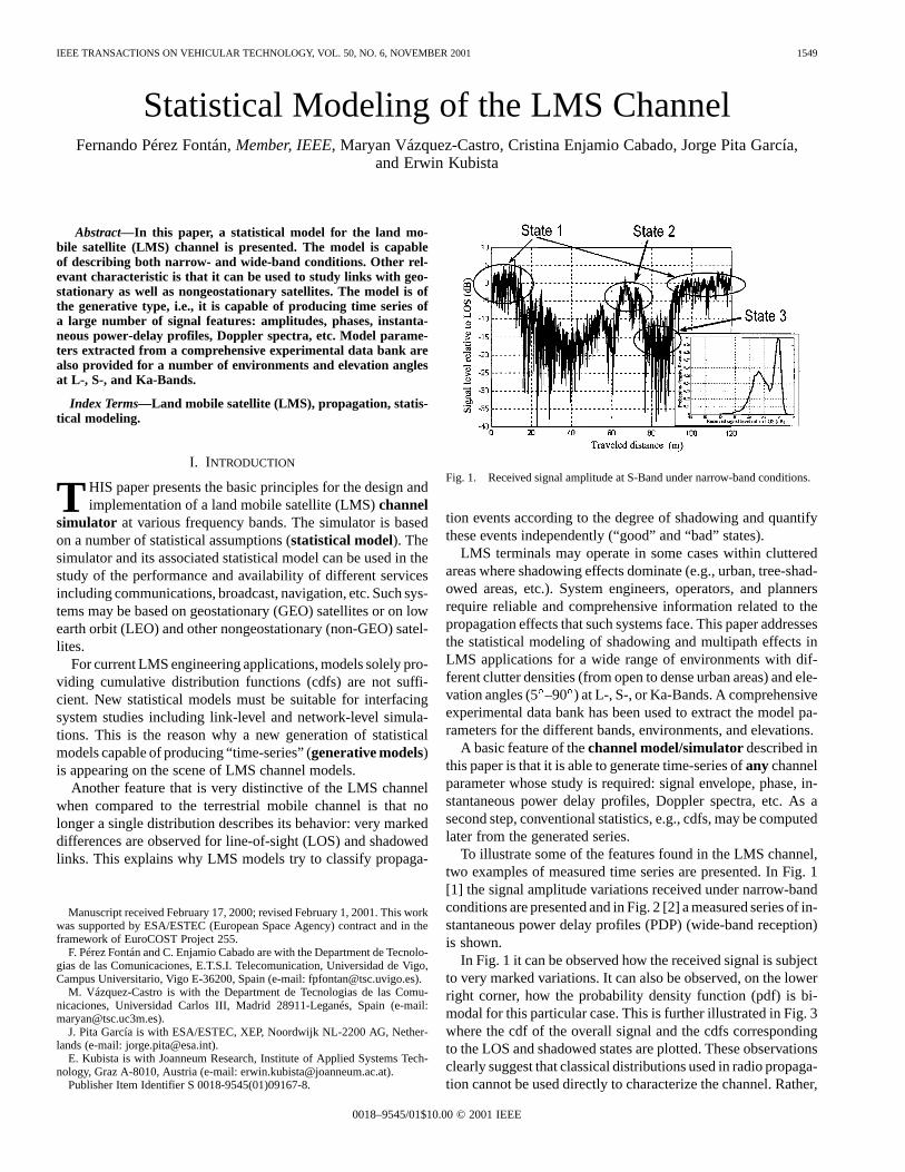
Fig. 1. Received signal amplitude at S-Band under narrow-band conditions.

tion events according to the degree of shadowing and quantifythese events independently (“good” and “bad” states).

LMS terminals may operate in some cases within clutteredareas where shadowing effects dominate (e.g., urban, tree-shad-owed areas, etc.). System engineers, operators, and plannersrequire reliable and comprehensive information related to thepropagation effects that such systems face. This paper addressesthe statistical modeling of shadowing and multipath effects inLMS applications for a wide range of environments with dif-ferent clutter densities (from open to dense urban areas) and ele-vation angles (5–90 ) at L-, S-, or Ka-Bands. A comprehensiveexperimental data bank has been used to extract the model pa-rameters for the different bands, environments, and elevations.

A basic feature of thechannel model/simulatordescribed inthis paper is that it is able to generate time-series ofany channelparameter whose study is required: signal envelope, phase, in-stantaneous power delay profiles, Doppler spectra, etc. As asecond step, conventional statistics, e.g., cdfs, may be computedlater from the generated series.

To illustrate some of the features found in the LMS channel,two examples of measured time series are presented. In Fig. 1[1] the signal amplitude variations received under narrow-bandconditions are presented and in Fig. 2 [2] a measured series of in-stantaneous power delay profiles (PDP) (wide-band reception)is shown.

In Fig. 1 it can be observed how the received signal is subjectto very marked variations. It can also be observed, on the lowerright corner, how the probability density function (pdf) is bi-modal for this particular case. This is further illustrated in Fig. 3where the cdf of the overall signal and the cdfs correspondingto the LOS and shadowed states are plotted. These observationsclearly suggest that classical distributions used in radio propaga-tion cannot be used directly to characterize the channel. Rather,

0018–9545/01$10.00 © 2001 IEEE

1550 IEEE TRANSACTIONS ON VEHICULAR TECHNOLOGY, VOL. 50, NO. 6, NOVEMBER 2001

Fig. 2. Measured instantaneous power delay profiles at L-Band. Wide-bandconditions.

Fig. 3. Overall received signal cdfs and cdfs for the LOS state (S1) and theheavy shadowed state (S3).

a combination of distributions is required; the overall pdf fol-lows the general expression given in

(1)

whereprobability that the link is in LOS conditions;pdf of the amplitude variations when in LOSconditions;probability of the link being under shadowedconditions;pdf of the signal variations when in shadowedconditions.

The previous approach is valid for the study of link budgetsin which standard link margins and availability levels are thewanted outcome. If, however, more detail is required, includingduration of different shadowing events or the time dispersioncaused by the channel and their influence on link and systemperformance, an approach capable of producing time-series isindicated. In this case, a model built around a Markov chain

has been selected to accomplish the goals stated throughout thissection.

In the context of channel modeling, the terms “echo” or “ray”are widely used. They indicate the different components givingrise to themultipath phenomenon. The electromagnetic fea-tures involved are described in a simplified way using this con-cept of echo, which is able to model fairly well the fast varia-tions and associated Doppler spread and the time dispersion inthe channel.

Fig. 2 shows that the channel not only causes signal ampli-tude variations but it also gives rise to time dispersion in the re-ceived signal, which, depending on the transmitted signal band-width, will cause distortion effects like frequency selectivity orintersymbol interference (ISI). These and other features of theLMS channel have to be accounted for in a suitable channelmodel/simulator.

Finally, the LMS channel may present significant differencesdepending on the elevation angle and the environment where themobile terminal is located. If GEO satellites are used, relativelylow elevation angles are found, especially for the northern lati-tudes. Other orbits such as LEO or medium earth orbits (MEO)or highly elliptical orbits (HEO) provide higher elevation anglesfor satellite-to-mobile transmissions, thus making it possible toovercome, in part, the shadowing effects caused by man-madeand/or natural features in the vicinity of the mobile. This eleva-tion angle dependence has also to be accounted for in a suitablemodel.

II. M ODEL AND SIMULATOR BASICS

The elements making up the signal received through the LMSchannel are thedirect ray and themultipath . Both the timeand locations variability and the time dispersion introduced bythe channel have to be accurately characterized. An importantfeature to be included in newer LMS models is the possibilityto account for both mobile and satellite movement along theirrespective trajectories.

The model presented in this paper is of the statistical type,this means that assumptions have to be made in which givenstatistical distributions are used to describe the various physicalphenomena affecting the direct signal and the multipath. In thisrespect, a first-order Markov chain [3]–[5] is used here to de-scribe the slow variations of the direct signal, basically due toshadowing/blockage effects. The overall signal variations due toshadowing and multipath effects within each individual Markovstate are assumed to follow a Loo [6] distribution with differentparameters for each shadowing condition (Markov state).

Up to this point the model is of thenarrow-band type sinceit does not account for time dispersion effects. These effects areintroduced by using anexponential distribution to representtheexcess delaysof the different echoes [7].

Different operational situations have been identified de-pending on the type of satellite and mobile user. These differentsituations will involve slightly different simulator implementa-tions. The following cases have been identified.

Case 1) stationary satellite and stationary mobile;Case 2) stationary satellite and moving mobile;Case 3) moving satellite and stationary mobile;

PÉREZ FONTÁNet al.: STATISTICAL MODELING OF THE LMS CHANNEL 1551

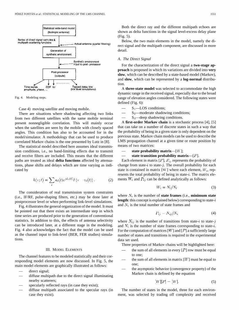
Fig. 4. Modeling steps.

Case 4) moving satellite and moving mobile.There are situations where shadowing affecting two links

from two different satellites with the same mobile terminalpresent nonnegligible correlation. This will mainly occurwhen the satellites are seen by the mobile with closely spacedangles. This condition has also to be accounted for in themodel/simulator. A methodology that can be used to producecorrelated Markov chains is the one presented by Lutz in [8].

The statistical model described here assumes ideal transmis-sion conditions, i.e., no band-limiting effects due to transmitand receive filters are included. This means that the differentpaths are treated as idealdelta functions affected by attenua-tions, phase shifts and delays which are time varying as indi-cated by

(2)

The consideration of real transmission system constraints(i.e., IF/RF, pulse-shaping filters, etc.) may be done later atpostprocessor level or when performing link-level simulations.

Fig. 4 illustrates the general organization of the model. It mustbe pointed out that there exists an intermediate step in whichtime series are produced prior to the generation of conventionalstatistics. In addition to this, the effects of antenna selectivitycan be introduced later, at a different stage in the modeling.Fig. 4 also acknowledges the fact that the model can be usedas the channel input to link-level (BER, FER studies) simula-tions.

III. M ODEL ELEMENTS

The channel features to be modeled statistically and their cor-responding model elements are now discussed. In Fig. 5, themain model elements are graphically illustrated as follows:

— direct signal;— diffuse multipath due to the direct signal illuminating

nearby scatterers;— specularly reflected rays (in case they exist);— diffuse multipath associated to the specular rays (in

case they exist).

Both the direct ray and the different multipath echoes areshown as delta functions in the signal level-excess delay plane(Fig. 5).

Below, the two main elements in the model, namely the di-rect signal and the multipath component, are discussed in moredetail.

A. The Direct Signal

For the characterization of the direct signal atwo-stage ap-proach is proposed in which its variations are divided intoveryslow, which can be described by a state-based model (Markov),andslow, which can be represented by alog-normal distribu-tion.

A three-state modelwas selected to accommodate the highdynamic range in the received signal, especially due to the broadrange of elevation angles considered. The following states weredefined (Fig. 6):

— S —LOS conditions;— S —moderate shadowing conditions;— S —deep shadowing conditions.A first-order Markov chain is a stochastic process [4], [5]

that can take on a number of discrete states in such a way thatthe probability of being in a given state is only dependent on theprevious state. Markov chain models can be used to describe theLMS propagation channel at a given time or route position bymeans of two matrices:

— state probability matrix —[ ];— state transition probability matrix —[ ].Each element in matrix [], represents the probability of

change from state-to state-. The overall probability for eachstate is contained in matrix [ ] where each element, , rep-resents the total probability of being in state-. The matrix ele-ments and can be defined analytically as follows:

(3)

where is the number ofstate frames(i.e., minimum statelength: this concept is explained below) corresponding to state-and is the total number of state frames and

(4)

where is the number of transitions from state-to state-and is the number of state frames corresponding to state-.For the computation of matrices [] and [ ] a sufficiently largenumber of states and transitions is required in the experimentaldata set used.

Three properties of Markov chains will be highlighted here:

— the sum of all elements in every [] row must be equalto one;

— the sum of all elements in matrix [ ] must be equal toone;

— the asymptotic behavior (convergence property) of theMarkov chain is defined by the equation

(5)

The number of states in the model, three for each environ-ment, was selected by trading off complexity and received


Fig. 5. Main model elements.

Fig. 6. Three-state model used to describe the dynamics of the direct signal.

signal dynamic range for every environment and elevationangle, taking into account that the model has to describe verydifferent situations ranging from very cluttered areas at lowelevations to open areas at very high elevation angles.

Typically, each state will last a few meters along the traveledroute. In [9] aminimum state length or state frameof 3–5 m was observed in the analysis of a large experimentalS-Band data set [1]. The definition of a minimum state lengthaffects the generation of direct signal series: a new state willbe drawn randomly every time the mobile travels a distanceof meters. The triggering of the Markov engine (or en-gines) is discussed later in more detail.

The model makes the simplifying assumption of the existenceof three basic rates of change (very slow, slow and fast) in thereceived signal corresponding to the different behaviors of itscomponents.States represent different gross shadowing con-ditions, e.g., if the mobile goes from being behind a tree or abuilding to being in the clear LOS of the transmitter. These sit-uations correspond to different states. The marked signal varia-tions due to state changes are considered as thevery slow varia-tionsof the direct signal and, consequently, of the overall signal.

As for the slow variations, they represent small-scalechanges in the shadowing attenuation produced as the mobiletravels in the shadow of the same obstacle: shadowing varia-tions behind a group of trees due to different leaf and branch

Fig. 7. Different rates of change of the various received signal components.

densities or shadowing variations behind a single building orgroup of buildings. In the LOS state, slow variations may bedue to different reasons: nonuniform receive antenna patternsand/or changes in mobile orientation with respect to thesatellite.

An element in the modeling of the slow variations lacking suf-ficient reported data is thecorrelation distance, , (Fig. 7).This parameter describes how fast the log-normally distributedvariations are values in the order of 1–3 m have been ob-served [9]. The autocorrelation properties of the very slow vari-ations are implicitly present in the Markov chain (transition ma-trices) and in the state frame concept.

B. The Multipath Component

Multipath contributions can be broken down into two classes:those originating from the direct ray (i.e., those echoes gen-erated by the direct signal’s illumination of scatterers in thevicinity of the mobile terminal) and those due to specular rays,if they exist. Few strong, far-echo events (existence of specularrays) have been recorded in the experimental data sets analyzed,as indicated later in Section V.

Undernarrow-band conditions, i.e., when multipath echoesare not significantly spread in time, for the modeling of thediffuse contributions, the most commonly used parameter is


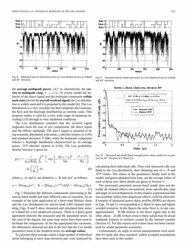
Fig. 8. Measured narrow-band time-series in a tree-shadowed area at S-Bandand 40 elevation.

the average multipath power, or, alternatively, thecar-rier-to-multipath ratio , . To jointly model the be-havior of the direct signal and the multipath componentwithineach state(not for theoverall received signal) the Loo distribu-tion is widely used and it is proposed in this model [6]. The Loodistribution is a very versatile one that comprises the Gaussian,the Rice and the Rayleigh distributions as extreme cases. Thisproperty makes it valid for a very wide range of situations in-cluding LOS through to very shadowed conditions.

The Loo distribution considers that the received signaloriginates from the sum of two components: the direct signaland the diffuse multipath. The direct signal is assumed to belog-normally distributed with mean (decibel relative to LOS)and standard deviation (dB), while the multipath componentfollows a Rayleigh distribution characterized by its averagepower, (decibel relative to LOS). The Loo probabilitydensity function is given by

(6)

where and are related to and as follows:

(7)Fig. 7 illustrates the different components intervening in the

narrow-band model and their different rates of variation. As anexample of the joint application of a three-state Markov chainand the Loo distribution for narrow-band LMS channel mod-eling, Figs. 8 and 9 show measured and simulated time seriesat S-Band for a tree shadowed scenario. There is a fairly goodagreement between the measured and the simulated series. Inthe case of the figures, the same state series have been used tofacilitate the comparison. As for the superposed fast variations,the differences observed are due to the fact that the Loo modelparameters used in the modeled series areaverage values.

To calculate these average values a large number of individualseries belonging to each state-elevation pair were analyzed by

Fig. 9. Simulated narrow-band time-series in a tree-shadowed area at S-Bandand 40 elevation.

Fig. 10. Measured and model fitted averaged power delay profile for an openarea for 80 elevation at L-Band [2].

calculating their individual cdfs. Then each measured cdfs wasfitted to the Loo distribution, thus obtaining sets of and

values. The values of the parameters finally used in themodel, and given tabulated form later, are the average values ofeach of those sets. More details are given in Section V.

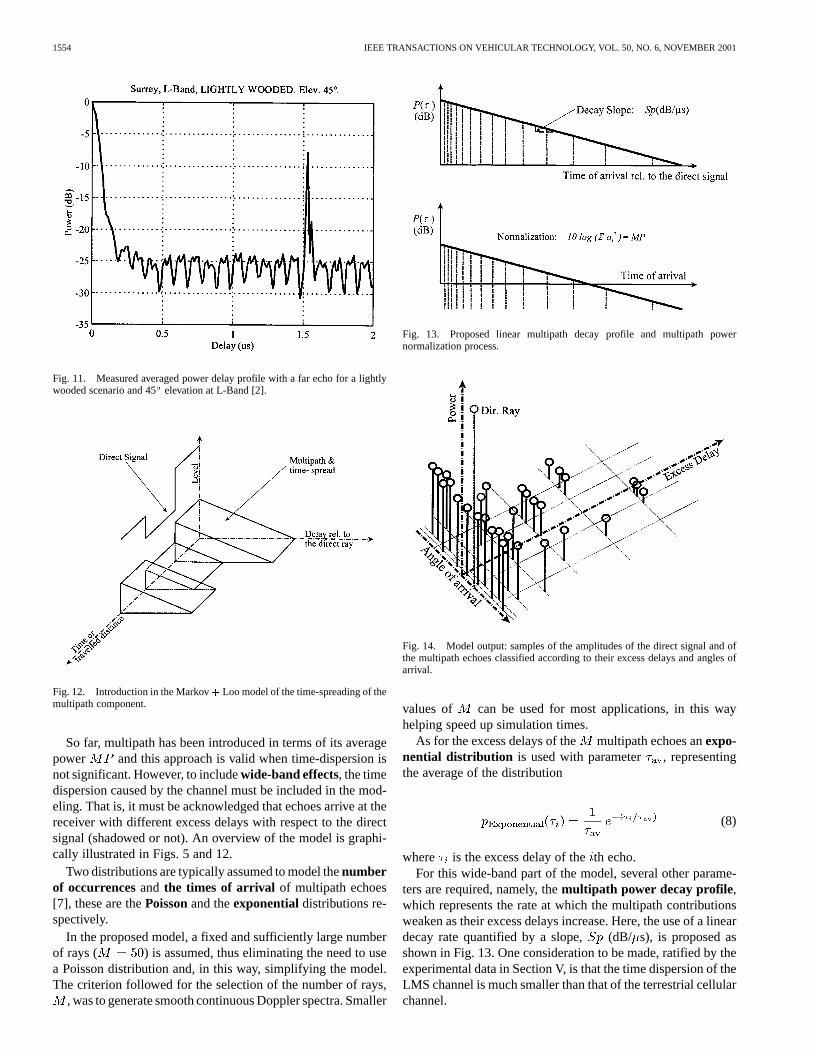
The previously presented narrow-band model does not de-scribe all channel effects encountered, more specifically, timeand angle of arrival dispersion. In this respect, experimental datawas available where time-dispersion effects could be observed.Examples of measured power delay profiles (PDPs) are shownin Figs. 10 and 11 corresponding to L-Band in open and lightlywooded scenarios. In the figures the noise floor is, in one case,approximately 30 dB relative to the direct signal and, in theother, about 25 dB. Echoes close to these values may be actualmultipath features or artifacts caused by the channel sounder(Section V). For this reason such echoes have not been consid-ered for model parameter extraction.

Unfortunately, no angle of arrival measurements were avail-able for study and, thus, standard, widely accepted assumptionshave been used in this model.


Fig. 11. Measured averaged power delay profile with a far echo for a lightlywooded scenario and 45elevation at L-Band [2].

Fig. 12. Introduction in the Markov+ Loo model of the time-spreading of themultipath component.

So far, multipath has been introduced in terms of its averagepower and this approach is valid when time-dispersion isnot significant. However, to includewide-band effects, the timedispersion caused by the channel must be included in the mod-eling. That is, it must be acknowledged that echoes arrive at thereceiver with different excess delays with respect to the directsignal (shadowed or not). An overview of the model is graphi-cally illustrated in Figs. 5 and 12.

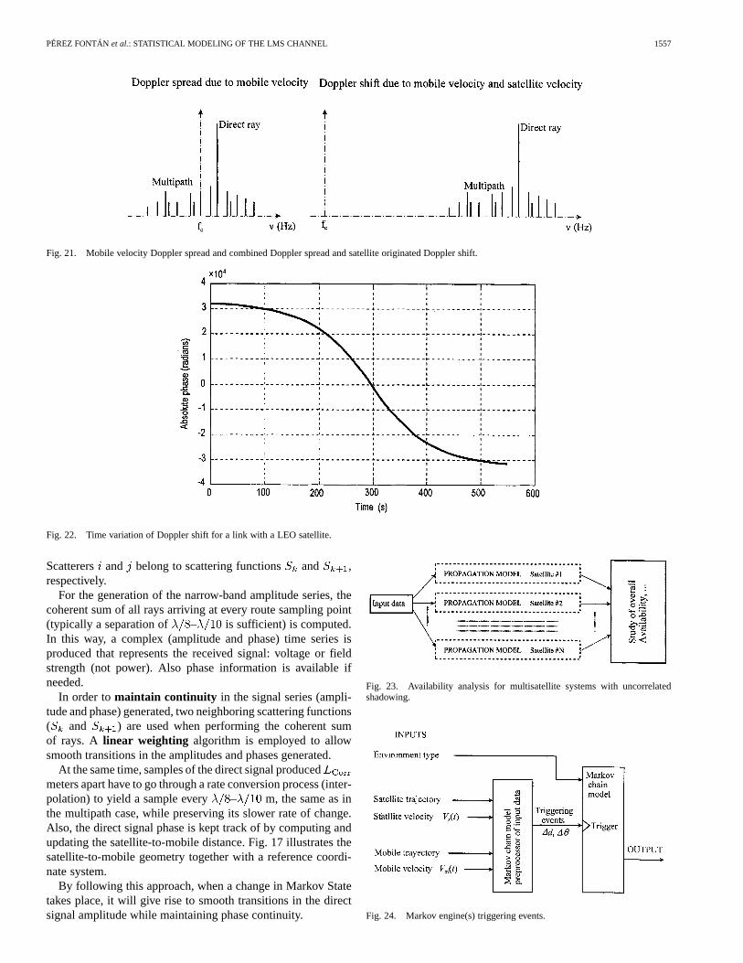
Two distributions are typically assumed to model thenumberof occurrencesand the times of arrival of multipath echoes[7], these are thePoissonand theexponentialdistributions re-spectively.

In the proposed model, a fixed and sufficiently large numberof rays ( ) is assumed, thus eliminating the need to usea Poisson distribution and, in this way, simplifying the model.The criterion followed for the selection of the number of rays,

, was to generate smooth continuous Doppler spectra. Smaller

Fig. 13. Proposed linear multipath decay profile and multipath powernormalization process.

Fig. 14. Model output: samples of the amplitudes of the direct signal and ofthe multipath echoes classified according to their excess delays and angles ofarrival.

values of can be used for most applications, in this wayhelping speed up simulation times.

As for the excess delays of the multipath echoes anexpo-nential distribution is used with parameter , representingthe average of the distribution

(8)

where is the excess delay of theth echo.For this wide-band part of the model, several other parame-

ters are required, namely, themultipath power decay profile,which represents the rate at which the multipath contributionsweaken as their excess delays increase. Here, the use of a lineardecay rate quantified by a slope, (dB/ s), is proposed asshown in Fig. 13. One consideration to be made, ratified by theexperimental data in Section V, is that the time dispersion of theLMS channel is much smaller than that of the terrestrial cellularchannel.


Fig. 15. Generation of synthetic scenarios consisting of point scatterers belonging to two consecutive scattering functions like the one in Fig. 14.

As indicated in Fig. 13, the total average power of themul-tipath rays (power sum) must be equal to (average multi-path power)

dB (9)

where is the amplitude of theth multipath echo. The previousexpression allows for the appropriatenormalization of the rel-ative powers of the direct and multipath components. The con-vention throughout is that LOS conditions imply a direct signalamplitude of 1 or 0 dB [ ].

It should be clarified at this point that the parameterdescribes the diffuse multipath power generated by the directsignal illuminating the environment in the vicinity of the mobile(near echoes). values extracted from experimental data aretabulated in Section V.Far echoes, in case they exist, must beintroduced separately in the model and, hence, they do not affectthe value of . As indicated later in Section V the number ofevents in which far echoes were recorded is not large enough toextract significant model parameters out of the available exper-imental data sets.

This statistical model has to be complemented with one fur-ther element, namely, thedistribution of angles of arrival ofthe multipath echoes. Due to lack of experimental data it is pro-posed that auniform azimuth distribution be employed fornear echoes. This assumption is realistic and widely used inother models.

IV. M ODEL OUTPUTS

Themodel output consists of two elements:

1) a series of direct signal (amplitude and phase) variationssampled every meters;

2) for multipath echoes, a series of pointscattering func-tions, (stored channel file), sampled in themobile traveled distance domain every meters

[or time domain for cases 1) and 3), Section II, when themobile is stationary and the satellite is moving]. Thesefunctions contain the complex amplitudes of the multi-path echoes classified according to their excess delaysand angles of arrival ( ).

The value of has to be chosen so as to fulfill the wide-sense stationary (WSS) assumption. Values of a few meters arewidely reported in the literature.

Fig. 14 schematically illustrates one entry to the storedchannel file produced at this stage in the modeling. In ansubsequent step (Fig. 4), from of these outputs, syntheticscenarios are created geometrically as illustrated in Fig. 15.These scenarios are made up of point isotropic scatterers givingrise to multipath echoes whose amplitudes, delays and anglesof arrival have already been generated with the aid of thestatistical distributions outlined earlier and contained in the

functions previously generated.The main purpose of generatingsynthetic scenariosis to re-

produce the ray interference effects due to path changes (andassociated phase changes) as the mobile and the satellite moveby keeping track of the varying distances from the satellite to thescatterers and from the scatterers to the mobile. This modelingapproach, although statistical, introduces a geometrical compo-nent which is very intuitive and helps to reproduce phase effectsdue to path length changes caused by the mobile and satellite dy-namics. It also has the advantage of the possible reuse of simu-lation runs for different receiver antenna patterns (flow diagramin Fig. 4).

To clarify the use ofthe synthetic scenario approach, twopostprocessing tasks, namely, the procedures for the generationof narrow-band received signal time series and the generationof Doppler shift time series are presented below.

A. Generation of Narrow-Band Time-Series

To show how the model outputs [direct signal series and seriesof multipath point scattering functions, , and their


Fig. 16. Combination of rays belonging to consecutive synthetic scenarios to generate complex-envelope time series.

Fig. 17. Satellite-to-mobile geometry and reference coordinate system.

Fig. 18. Example of generated signal amplitude series.

associated synthetic scenarios] may be processed to producemeaningful information, the generation process of narrow-bandamplitude series is explained with the aid of Figs. 15 and 16 forcase 2)(stationary satellite and moving mobile).

Fig. 19. Example of generated phase series corresponding to the samesimulation as Fig. 18.

Fig. 20. Phase change/Doppler generation geometry.

In the figures, for two neighboring points along the mobileroute ( and ) synthetic scenarios corresponding to twoconsecutive scattering functions, and

are created as a first step. In Fig. 16 two scat-terers, and , generated for route pointsand are shown.


Fig. 21. Mobile velocity Doppler spread and combined Doppler spread and satellite originated Doppler shift.

Fig. 22. Time variation of Doppler shift for a link with a LEO satellite.

Scatterers and belong to scattering functions and ,respectively.

For the generation of the narrow-band amplitude series, thecoherent sum of all rays arriving at every route sampling point(typically a separation of – is sufficient) is computed.In this way, a complex (amplitude and phase) time series isproduced that represents the received signal: voltage or fieldstrength (not power). Also phase information is available ifneeded.

In order tomaintain continuity in the signal series (ampli-tude and phase) generated, two neighboring scattering functions( and ) are used when performing the coherent sumof rays. A linear weighting algorithm is employed to allowsmooth transitions in the amplitudes and phases generated.

At the same time, samples of the direct signal producedmeters apart have to go through a rate conversion process (inter-polation) to yield a sample every – m, the same as inthe multipath case, while preserving its slower rate of change.Also, the direct signal phase is kept track of by computing andupdating the satellite-to-mobile distance. Fig. 17 illustrates thesatellite-to-mobile geometry together with a reference coordi-nate system.

By following this approach, when a change in Markov Statetakes place, it will give rise to smooth transitions in the directsignal amplitude while maintaining phase continuity.

Fig. 23. Availability analysis for multisatellite systems with uncorrelatedshadowing.

Fig. 24. Markov engine(s) triggering events.


Fig. 25. A change in Markov engine due to a 10change in elevation is assumed to be accompanied by a new random state draw.

TABLE IAVAILABLE DATABASES AND THEIR CHARACTERISTICS

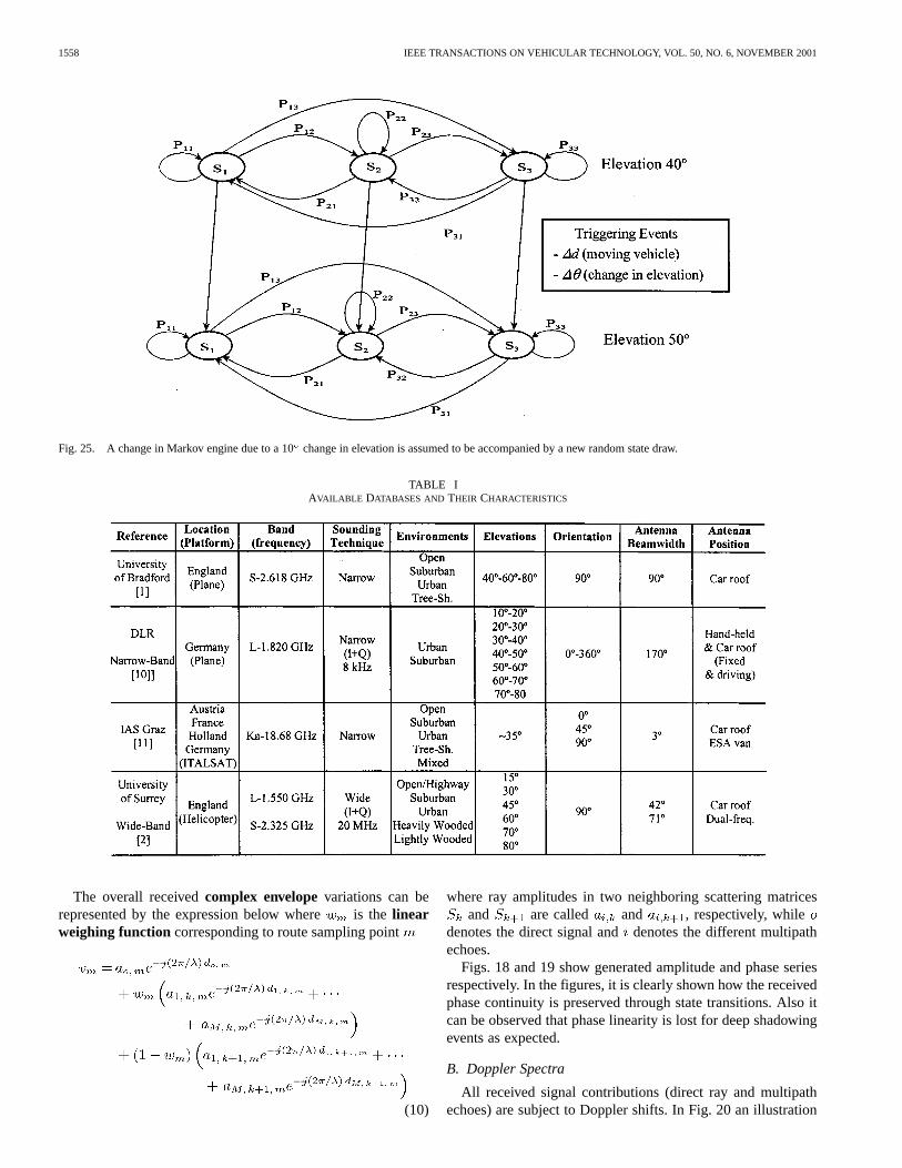
The overall receivedcomplex envelopevariations can berepresented by the expression below where is the linearweighing function corresponding to route sampling point

(10)

where ray amplitudes in two neighboring scattering matricesand are called and , respectively, while

denotes the direct signal anddenotes the different multipathechoes.

Figs. 18 and 19 show generated amplitude and phase seriesrespectively. In the figures, it is clearly shown how the receivedphase continuity is preserved through state transitions. Also itcan be observed that phase linearity is lost for deep shadowingevents as expected.

B. Doppler Spectra

All received signal contributions (direct ray and multipathechoes) are subject to Doppler shifts. In Fig. 20 an illustration


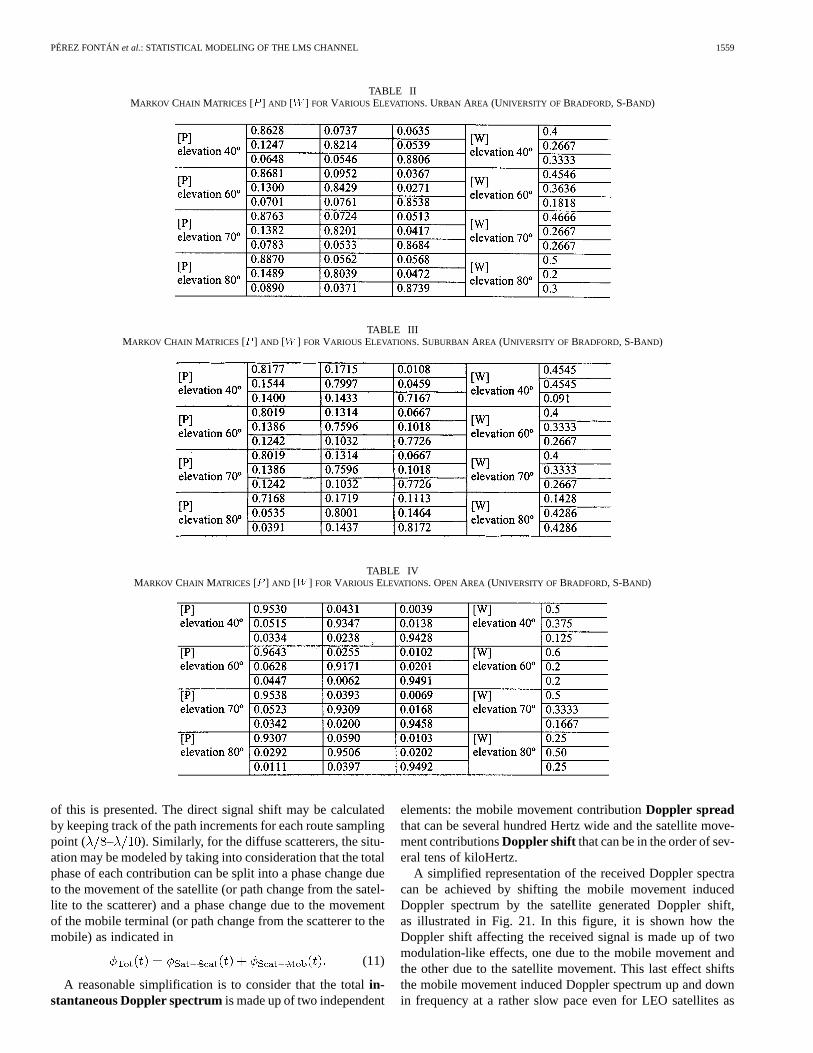
TABLE IIMARKOV CHAIN MATRICES [P ] AND [W ] FOR VARIOUS ELEVATIONS. URBAN AREA (UNIVERSITY OF BRADFORD, S-BAND)

TABLE IIIMARKOV CHAIN MATRICES [P ] AND [W ] FOR VARIOUS ELEVATIONS. SUBURBAN AREA (UNIVERSITY OF BRADFORD, S-BAND)

TABLE IVMARKOV CHAIN MATRICES [P ] AND [W ] FOR VARIOUS ELEVATIONS. OPEN AREA (UNIVERSITY OF BRADFORD, S-BAND)

of this is presented. The direct signal shift may be calculatedby keeping track of the path increments for each route samplingpoint ( – ). Similarly, for the diffuse scatterers, the situ-ation may be modeled by taking into consideration that the totalphase of each contribution can be split into a phase change dueto the movement of the satellite (or path change from the satel-lite to the scatterer) and a phase change due to the movementof the mobile terminal (or path change from the scatterer to themobile) as indicated in

(11)

A reasonable simplification is to consider that the totalin-stantaneous Doppler spectrumis made up of two independent

elements: the mobile movement contributionDoppler spreadthat can be several hundred Hertz wide and the satellite move-ment contributionsDoppler shift that can be in the order of sev-eral tens of kiloHertz.

A simplified representation of the received Doppler spectracan be achieved by shifting the mobile movement inducedDoppler spectrum by the satellite generated Doppler shift,as illustrated in Fig. 21. In this figure, it is shown how theDoppler shift affecting the received signal is made up of twomodulation-like effects, one due to the mobile movement andthe other due to the satellite movement. This last effect shiftsthe mobile movement induced Doppler spectrum up and downin frequency at a rather slow pace even for LEO satellites as


TABLE VMARKOV CHAIN MATRICES [P ] AND [W ] FORVARIOUS ELEVATIONS. INTERMEDIATE TREE SHADOWED AREA (UNIVERSITY OF BRADFORD, S-BAND)

TABLE VIMARKOV CHAIN MATRICES [P ] AND [W ] FOR VARIOUS ELEVATIONS. HEAVY TREESHADOWED AREA (UNIVERSITY OF BRADFORD, S-BAND)

TABLE VIIAVERAGE LOO MODEL PARAMETERS FORDIFFERENTELEVATIONS AND DIFFERENTSTATES (UNIVERSITY OF BRADFORD, S-BAND)

shown in Fig. 22, where an example for a polar orbit LEOsatellite is presented.

V. SIMULATOR IMPLEMENTATION ISSUES

In previous sections, the basic model elements have been de-scribed, now the adequate sequencing of all these elements into

a channel simulator is presented. As indicated in the Introduc-tion (Section I) the approach followed is to generate time-seriesof the different elements in the received signal—direct ray andmultipath—and combine them suitably at the receiver takinginto consideration their distributions and their relative rates ofchange, i.e., slow and fast variations. Apostprocessoris re-quired to produce the relevant received signal statistics from the


TABLE VIIIMARKOV CHAIN MATRICES [P ] AND [W ] FORVARIOUS ELEVATIONS. NARROW-BAND, URBAN AREA, VEHICLE MOUNTED ANTENNA (DLR, L-BAND)

TABLE IXAVERAGE LOO MODEL PARAMETERS FORDIFFERENT ELEVATIONS AND DIFFERENT STATES. NARROW-BAND, URBAN AREA, VEHICLE

MOUNTED ANTENNA (DLR, L-BAND)

TABLE XMARKOV CHAIN MATRICES [P ] AND [W ] FORVARIOUS ELEVATIONS. NARROW-BAND, SUBURBAN AREA, VEHICLE MOUNTED ANTENNA (DLR, L-BAND)


TABLE XIAVERAGE LOO MODEL PARAMETERS FORDIFFERENT ELEVATIONS AND DIFFERENT STATES. NARROW-BAND, SUBURBAN AREA, VEHICLE

MOUNTED ANTENNA (DLR, L-BAND)

TABLE XIIMARKOV CHAIN MATRICES [P ] AND [W ] FORVARIOUS ELEVATIONS. NARROW-BAND, URBAN AREA, HAND-HELD ANTENNA (DLR, L-BAND)

generated time series, both for narrow- and wide-band condi-tions.

When investigating the combined behavior of a network con-sisting of a constellation of several satellites, the model must berun as many times as satellites in the constellation under study.The variations (very slow, slow, and fast) of the received signalsfrom the different satellites are considered to be uncorrelated(Fig. 23).

Only when the degree ofshadowing correlation is highenough (for small angle separations between two satellites) thecombined production of correlated time series is required. Thisspecial case will occur with a small likelihood. One possibleway to model situations where shadowing correlation is notnegligible is to use the methodology formulated by Lutz [8] forthe generation of correlated Markov chains.

The implementation of the describedmodel into a practicalchannelsimulator presents additional complexities not foundin the terrestrial mobile case. These are due to the fact that notonly the mobile is capable of changing its position with time butalso that the satellites may move at high speeds, e.g., LEO satel-lites. There even exists the case in which it is only the satellite

that moves while the mobile is stationary. The special case inwhich both the satellite and the mobile are stationary must alsobe addressed.

This is the reason why, in the model/simulator, special atten-tion must be paid to apreprocessingtask in which the posi-tions along the mobile route and the satellite trajectory as well asthe instants when a state change event may occur are identified.Different triggering eventsmust be considered for the differentphenomena accounted for in this model. Below, the implicationsinvolving each of the model elements are analyzed.

The direct signal is assumed to undergovery slowvariationsalong the route. These variations are modeled by means of aMarkov chain model. In a first, narrow-band version of thismodel [5] a minimum state length calledFrame was alreadyconsidered. Thus, for every meters along the mobileroute a draw of a random number has to be made to trigger thecurrent Markov chain engine. This is valid for the case where thesatellite is stationary (GEO) and the mobile is moving. However,the situation in which the satellite is moving while the mobile isstationary must also be accounted for. For such situations, addi-tional triggering events must be considered (Fig. 24).


TABLE XIIIAVERAGE LOO MODEL PARAMETERS FORDIFFERENT ELEVATIONS AND DIFFERENT STATES. NARROW-BAND, URBAN AREA,

HAND-HELD ANTENNA (DLR, L-BAND)

TABLE XIVMARKOV CHAIN MATRICES [P ] AND [W ] FORVARIOUS ELEVATIONS. NARROW-BAND, SUBURBAN AREA, HAND-HELD ANTENNA (DLR, L-BAND)

TABLE XVAVERAGE LOO MODEL PARAMETERS FORDIFFERENT ELEVATIONS AND DIFFERENT STATES. NARROW-BAND, SUBURBAN AREA,

HAND-HELD ANTENNA (DLR, L-BAND)

Few measured data are available to quantify this. However,it is clear that state changes can be triggered by changes inthe satellite elevation and/or azimuth with respect to a sta-tionary/moving terminal. Here it is assumed that state changesmay be triggered by changes in elevation,, in addition tochanges in the mobile position, (every meters).

As for the changes in elevation, , the Markov model isstructured around engines valid for elevation ranges of 10, i.e.,the Markov model uses different matrices [] and [ ] for dif-ferent elevations: 10 , 40 , 50 , 60 .

Whenever a change in Markov engine occurs, for example,from that of 40 to that of 50 , a new draw of a random number

has to be made to decide whether a change in state in addition toa change in Markov engine has occurred. This is illustrated withthe aid of Fig. 25. Both direct signal and multipath conditions(model parameters [ ], [ ], ) will change fordifferent Markov engines (different elevations) and for differentstates.

VI. M ODEL PARAMETERS

In this section, the parameters for the model/simulator de-scribed in the previous sections are presented. These parame-ters have been extracted from part of the ESA/ESTEC (Euro-


TABLE XVIAVERAGE LOO MODEL PARAMETERS FORDIFFERENTORIENTATIONS AND SIDES OF THEROAD (IAS, GRAZ, Ka-BAND)

pean Space Agency) LMS measurement database. Table I sum-marizes the main features of the measurement campaigns andavailable experimental data.

A. Narrow-Band Model Parameters

The data from the University of Bradford, U.K., was obtainedunder narrow-band conditions at S-Band [1]. The data consistsof a comprehensive set for several environments: open, sub-urban, urban, tree-shadowed, and elevations: 40, 60 , 70 and80 . Flights were parallel to the road. Radio paths were, thus,orthogonal to the route (orientation 90). Measurements werecarried out with a carrier frequency of 2618 MHz. The parame-ters extracted from the data set are summarized in Tables II–VII.

The DLR (Germany) data set is narrow-band and was ob-tained at L-band (1820 MHz) both for hand-held and car-roofantennas and both for stationary as well as moving vehicle con-ditions [10]. The airplane carrying the transmitter flew in circlesaround the receiver. The model parameters extracted from thisdata set are summarized in Tables VIII–XV.

The IAS (Austria) data was obtained at Ka-Band using theItalsat satellite for a fixed elevation of 30–35 and orientationsof approximately 0, 45 , and 90 [11]. Satellite side (Sat) andopposite side (Opp) of the road runs were available for anal-ysis. Since a directive antenna was used, only direct signal vari-ations (and little multipath) were available for analysis. The ex-tracted model parameters form this data set are summarized inTables XVI–XXI.

The extraction of model parameters in the above cases wasmade by plotting the cdfs of individual sections of the measuredseries (corresponding to specific states) and finding the Loo cdfthat more closely fitted the measured cdf. After this process alarge number of Loo distribution parameters ( ) wereavailable for each environment, elevation, and state. The param-eters shown in Tables XVI–XXI are averaged values.

B. Wide-Band Model Parameters

Wide-band data obtained from measurements using a slidingcorrelator channel sounder were analyzed. Two data sets fromthe university of Surrey, U.K., (L- and S-Bands) were studied.

From the measured data (series of instantaneous power delayprofiles, PDPs) corresponding to shadowed conditions (States 2and 3) it was observed that due to sounder power limitations, thedynamic range available was too small to “see” most delayedechoes. It was thus decided to carry out the wide-band study(model parameter fitting) only for LOS (State-1) paths.

This decision does not dramatically affect the possible useof this model for system performance and availability studies.

TABLE XVIIMARKOV CHAIN MATRICES [P ] AND [W ] FOR VARIOUS ELEVATIONS.

FRANCE, LEAF TREES,�30 ELEVATION (IAS, GRAZ, Ka-BAND)

LMS systems are typically implemented with small fademargins; this means that, once the received signal is below agiven threshold, i.e., when in states 2 and 3, system outage willoccur regardless of channel-time dispersion. As for LOS paths(State-1), potential situations of unavailability will only occurwhen the channel time dispersion is significant compared tothe inverse of the symbol rate.

The parameter fitting procedure is illustrated with the aidof Fig. 26. In order to compare measured and simulated PDPsthe internal signal processing in the channel sounder was emu-lated. Ideal instantaneous channel impulse responses (made upof delta functions) resulting from the channel model/simulatorwere passed through a filter representing the behavior and char-acteristics of the channel sounder.

A first step before performing profile fitting was to computethe average of various neighboring measured PDPs in orderto remove instantaneous multipath cancellation and enhance-ment effects (averaged power delay profiles, APDPs). A similarprocess was carried out for the simulated instantaneous PDPs.

Model parameter extraction, in this case, was also carried outby comparing measured and modeled APDPs: their shapes, theiraverage delays, and delay spreads. An example of model fittedAPDP is shown in Fig. 10. Model parameters for homogeneoussections of the measured PDPs corresponding to different envi-ronments and elevations were obtained. Finally, all the param-eters obtained for a given environment and elevation were av-


TABLE XVIIIMARKOV CHAIN MATRICES [P ] AND [W ] FOR VARIOUS ELEVATIONS.GERMANY NEEDLE TREES,�30 ELEVATION (IAS, GRAZ, Ka-BAND)

TABLE XIXMARKOV CHAIN MATRICES [P ] AND [W ] FOR VARIOUS ELEVATIONS.

AUSTRIA, TREE ALLEY,�30 ELEVATION (IAS, GRAZ, Ka-BAND)

eraged to provide a single value for each case considered (Ta-bles XXII and XXIII).

LOS power delay profiles were classified into the followingthree categories:

— type 1.A—representing those APDPs with no featuresother than in the first delay bin;

— type 1.B—representing those APDPs with additionalfeatures in delay bins 2, 3, 4, (i.e., with time dis-persion);

— type 2—those APDPs where long delays were ob-served (far echoes).

TABLE XXMARKOV CHAIN MATRICES [P ] AND [W ] FOR VARIOUS ELEVATIONS.

GERMANY/AUSTRIA, SUBURBAN,�30 ELEVATION (IAS, GRAZ, Ka-BAND)

TABLE XXIMARKOV CHAIN MATRICES [P ] AND [W ] FOR VARIOUS ELEVATIONS.

GERMANY, URBAN,�30 ELEVATION (IAS, GRAZ, Ka-BAND)

In the extraction of model parameters from these three profiletypes, the criteria presented below were followed.

— For 1.A profiles, no wide-band model fitting was pos-sible. The channel in this case may be considered to benarrow-band with respect to the characteristics of thechannel sounder employed. For this case, model pa-rameters obtained in narrow-band measurement cam-paigns can used (Tables II–XXI).

— For 1.B profiles, wide-band model fittings were per-formed and model parameters extracted. Also the oc-currence probabilities of profiles 1.A and 1.B havebeen recorded (Tables XXII and XXIII).


Fig. 26. Simulation of the channel sounder.

TABLE XXIIL-BAND SURREY. PDP TYPE OCCURRENCEPROBABILITIES

— Type 2 profiles occurred very seldom and its study isleft out of this paper pending further analysis.

The proposed APDP classification in types 1.A and 1.B (type2 may be, in a first approach, disregarded given its very lowoccurrence probability) suggest a possible way of extending thenarrow-band three-state Markov model to study wide-band con-ditions. In this enhanced model, only for the LOS state, theMarkov chain is modified to include a split state-1: S-1 non-depressive and S-1 depressive.

The Markov engine bounces back and forth from the non-depressive to the depressive states as illustrated in Fig. 27. Forthis wide-band model only occurrence probabilities have beenobtained form measurements but no reliable transition probabil-ities are yet available.

As indicated earlier, wide-band data from the Universityof Surrey, U.K., at L- and S-Band was analyzed. Radio-paths

were orthogonal with respect to the mobile route [2]. A channelsounder chip rate of 10 Mc/s was used with two different codelengths ( and ). Extracted parameters from thisdata set are listed in Tables XXII and XXIII.

VII. CONCLUSION

In this paper, a geometric-statistical model/simulator hasbeen presented and described. The model is based on theassumption of the existence on three different rates of changein the main propagation channel elements: the direct signal thatmay undergo shadowing/blockage effects and the multipath(specular and diffuse). These three rates of variation are de-scribed by means of a three-state Markov chain, a log-normaldistribution and the coherent sum of the direct ray and themultipath echoes, respectively. The model has been extended to


TABLE XXIIIL-BAND, SURREY. CLASS 1B PROFILES. FIT PARAMETERS ASSUMINGSp

(DECAY SLOPE) = 10 dB/�s

Fig. 27. Wide-band model.

describe both narrow- and wide-band conditions by assumingthat individual multipath ray excess delays are exponentiallydistributed. Model parameters have been extracted from acomprehensive measurement campaign at L-, S-, and Ka-Bandsfor a number of elevations and environments. A fairly goodagreement between measurements and model outputs hasbeen observed in all cases. Specific areas of further work havebeen identified mainly in the modeling of highly depressiveconditions in which a dual Markov model has been proposedfor LOS situations.

REFERENCES

[1] H. Smith, S. K. Barton, J. G. Gardiner, and M. Sforza, “Characterizationof the land mobile-satellite (LMS) channel at L and S bands: Narrow-band measurements,”, Bradford, ESA AOPs 104 433/114 473, 1992.

[2] B. G. Evans, G. Butt, M. J. Willis, and M. A. N. Parks, “Land mobilesatellite wideband measurement experiment at L- and S-bands,” Univer-sity of Surrey, ESA ESTEC Contract no. 10 528/93/NL/MB(SC), FinalRep., 1996.

[3] E. Lutz et al., “The land mobile satellite communicationchannel-recording, statistics, and channel model,”IEEE Trans.Veh. Technol., vol. 30, pp. 375–386, May 1991.

[4] B. Vucetic and J. Du, “Channel modeling and simulation in satellite mo-bile communication systems,”IEEE J. Select. Areas Commun., vol. 10,pp. 1209–1217, 1992.

[5] F. P. Fontan, J. Pereda, M. J. Sedes, M. A. V. Castro, S. Buonomo, andP. Baptista, “Complex envelope three-state Markov chain simulator forthe LMS channel,”Int. J. Satellite Commun., pp. 1–15, Jan. 1997.

[6] C. Loo, “A statistical model for land mobile satellite link,”IEEE Trans.Veh. Technol., vol. VT-34, pp. 122–127, Aug. 1985.

[7] A. Jahn, H. Bischl, and G. Heis, “Channel characterization of spreadspectrum satellite communications,” inProc. IEEE 4th Int. Symp.Spread Spectrum Techniques and Applications (ISSSTA’96), Mainz,Germany, Sept. 1996, pp. 1221–1226.

[8] E. Lutz, “A Markov model for correlated land mobile satellite channels,”Int. J. Satellite Commun., vol. 13, pp. 333–339, 1996.

[9] F. P. fontan, M. A. V. Castro, S. Buonomo, P. Baptista, and B. Arbesser-Rastburg, “S-band LMS propagation channel behavior for different en-vironments, degrees of shadowing and elevation angles,”IEEE Trans.Broadcasting, vol. 44, pp. 40–76, Mar. 1998.

[10] A. Jahn and E. Lutz, “Propagation Data and channel model for LMSsystems,”, Final Rep. ESA PO 141 742. DLR, 1995.

[11] F. Murr, S. Kastner-Puschl, B. Bolzano, and E. Kubista, “Land MobileSatellite narrowband propagation measurement campaign at Ka-Band,”,ESTEC Contract 9949/92/NL, Final Rep., 1995.

Fernando Pérez Fontán(M’96) was born in Vilagarcia de Arousa, Spain. Hereceived the Diploma (telecommunications engineering) and Ph.D.degrees fromthe Polytechnic University of Madrid, Spain, in 1982 and 1992, respectively.

He is a Senior Lecturer with the Telecommunications Engineering School,University of Vigo, Spain, where he teaches a graduate course on mobile com-munications. His main research interests are in the field of mobile propagationchannel modeling, especially mobile satellite, and in link- and network-levelperformance evaluation of terrestrial and satellite mobile and broadcast net-works.

Maryan Vázquez-Castrowas born in Vigo, Spain. She received the M.S. de-gree in telecommunications engineering in 1994 and the Ph.D. degree (cumlaude) in 1998, both from the University of Vigo.

Since 1998, she has been an Assistant Professor with the Theory of Signaland Communications Department, Carlos III University of Madrid, Spain. Herresearch interests are in the area of satellite channel modeling and spread spec-trum communication systems.

Cristina Enjamio Cabado received the Diploma degree in telecommunica-tions engineering from the University of Vigo, Spain, in 1999. She is currentlyworking toward the Ph.D. degree at the same university.

She is a part-time Research Student at the University of Portsmouth, U.K.Her main research interests are in the field of broad-band wireless access andpropagation in millimeter wavelengths.

Jorge Pita Garcíawas born in Madrid, Spain, in 1974. He received the Diplomadegree in telecommunications engineering from the University of Vigo, Spain,in 1998. He is currently working toward the Ph.D. degree at the same university.

Since 2000, he has been with the Wave Interaction and Propagation Section,European Space Agency (ESA), Noordwijk, The Netherlands.

Erwin Kubista received the Dipl. Ing. degree in telecommunications and elec-tronic engineering from the Technical University of Graz, Austria, in 1985.

From 1985 to 1989, his was a Research Assistant in the Department of Com-munications and Wave Propagation, Technical University of Graz, responsiblefor radiometer diversity data analysis and processing under the European SpaceAgency (ESA) and European Union (EU) contracts.

Statistical modeling of the LMS channel

Documents

Transcript of Statistical modeling of the LMS channel