Application of Gauss's theorem to quantify localized surface ...

Atmos. Meas. Tech., 10, 3345–3358, 2017https://doi.org/10.5194/amt-10-3345-2017© Author(s) 2017. This work is distributed underthe Creative Commons Attribution 3.0 License.

Application of Gauss’s theorem to quantify localized surfaceemissions from airborne measurements of wind and trace gasesStephen Conley1,6, Ian Faloona1, Shobhit Mehrotra1, Maxime Suard1, Donald H. Lenschow2, Colm Sweeney4,Scott Herndon3, Stefan Schwietzke4,5, Gabrielle Pétron4,5, Justin Pifer6, Eric A. Kort7, and Russell Schnell51Department of Land, Air, & Water Resources, University of California, Davis, CA 95616, USA2Mesoscale and Microscale Meteorology Laboratory, National Center for Atmospheric Research,Boulder, CO 80307, USA3Aerodyne Research, Inc, Billerica, MA 01821, USA4Cooperative Institute for Research in Environmental Sciences, University of Colorado, Boulder, CO 80305, USA5NOAA Earth System Research Laboratory, Boulder, CO, USA6Scientific Aviation, Inc., Boulder, CO, USA7Climate and Space Sciences and Engineering, University of Michigan, Ann Arbor, MI, USA

Correspondence to: Stephen Conley ([email protected], [email protected])

Received: 24 February 2017 – Discussion started: 18 April 2017Revised: 11 August 2017 – Accepted: 16 August 2017 – Published: 13 September 2017

Abstract. Airborne estimates of greenhouse gas emissionsare becoming more prevalent with the advent of rapid com-mercial development of trace gas instrumentation featuringincreased measurement accuracy, precision, and frequency,and the swelling interest in the verification of current emis-sion inventories. Multiple airborne studies have indicatedthat emission inventories may underestimate some hydrocar-bon emission sources in US oil- and gas-producing basins.Consequently, a proper assessment of the accuracy of theseairborne methods is crucial to interpreting the meaning ofsuch discrepancies. We present a new method of samplingsurface sources of any trace gas for which fast and pre-cise measurements can be made and apply it to methane,ethane, and carbon dioxide on spatial scales of ∼ 1000 m,where consecutive loops are flown around a targeted sourceregion at multiple altitudes. Using Reynolds decompositionfor the scalar concentrations, along with Gauss’s theorem, weshow that the method accurately accounts for the smaller-scale turbulent dispersion of the local plume, which is of-ten ignored in other average ”mass balance” methods. Withthe help of large eddy simulations (LES) we further showhow the circling radius can be optimized for the microme-teorological conditions encountered during any flight. Fur-thermore, by sampling controlled releases of methane andethane on the ground we can ascertain that the accuracy of

the method, in appropriate meteorological conditions, is of-ten better than 10 %, with limits of detection below 5 kg h−1

for both methane and ethane. Because of the FAA-mandatedminimum flight safe altitude of 150 m, placement of the air-craft is critical to preventing a large portion of the emissionplume from flowing underneath the lowest aircraft samplingaltitude, which is generally the leading source of uncertaintyin these measurements. Finally, we show how the accuracy ofthe method is strongly dependent on the number of samplingloops and/or time spent sampling the source plume.

1 Introduction

Accurate national inventories of greenhouse gas emissions(primarily carbon dioxide – CO2; methane – CH4; and ni-trous oxide – N2O) is of paramount importance in devel-oping strategies to understand global emissions. The mul-titude of sources, however, are so often highly variable inarea, emission magnitude, height above ground, and dura-tion that rigorous verification is exceedingly difficult. Never-theless, measurement techniques have improved markedly inthe past decade, and these are being employed to an unprece-dented extent in an effort to evaluate and refine emission in-ventories (Nisbet and Weiss, 2010). Most so-called “bottom-

Published by Copernicus Publications on behalf of the European Geosciences Union.

3346 S. Conley et al.: Application of Gauss’s theorem to quantify localized surface emissions

up” inventories are developed by aggregating statistical cor-relates of individual process emissions to such mapping vari-ables as population density, energy consumption, head of cat-tle, etc., extrapolating to total emissions using a relativelysmall number of direct measurements. On the other hand, at-mospheric scientists have long striven to use measurementsfrom global surface networks, aircraft campaigns, and satel-lites to try to determine emissions based on the amounts andbuild-up rates of observed trace gases. Aircraft and satellites,the “top-down” approach, conveniently integrates the multi-tude of sources, but is heavily reliant on a detailed knowl-edge of atmospheric transport. Top-down methods also suf-fer from difficulties attributing sources and generalizing mea-surements made over a relatively short time period. Attemptsto reconcile these two distinct methods on global (Muhle etal., 2010) and continental scales (Gerbig et al., 2003; Milleret al., 2013) have often indicated an apparent underestima-tion by the bottom-up methods of a factor 1.5 or more.

In principle, the aircraft top-down measurements can beconducted at all the atmospheric scales to better understandand identify the emissions at comparable scales. For long-lived greenhouse gases, which readily disperse throughoutthe atmosphere, the global scale is very instructive. Theseminal experiment began with Keeling’s acclaimed CO2curve (1960), and has continued through more contemporarytechniques by Hirsch et al. (2006) and Neef et al. (2010) forCH4 and N2O, respectively. At progressively smaller scalesmore details of the source strengths and apportionment canbe made: from synoptic or continental scales which can helpconstrain national inventories (Bergamaschi et al., 2005) orspecific biogeographic regions (Gallagher et al., 1994), tomesoscale investigations that estimate emissions from urbanareas (Mays et al., 2009; Turnbull et al., 2011; Wecht et al.,2014) or specific oil- and gas-producing fields (Karion etal., 2013; Petron et al., 2014) and even down to individualpoint/area sources on the order of 10–100 m size (Denmeadet al., 1998; Lavoie et al., 2015; Roscioli et al., 2015).

Aircraft in situ measurements are particularly useful fortop-down methods at the sub-mesoscale because they canbe used to measure the air both upwind and downwind ofa source region. However, deployments tend to be costly andthus sporadic. As far as we know, the aircraft methods usedso far can be categorized into three types. First, there is theeddy covariance technique that is carried out at low altitudeswherein the vertical fluxes of gases carried by the turbulentwind are measured by tracking rapid fluctuations of both con-centrations and vertical wind (Hiller et al., 2014; Ritter et al.,1994; Yuan et al., 2015). This method is generally thoughtto be the most direct, but it is limited to small footprint re-gions which must be repeatedly sampled for sufficient statis-tical confidence, requires a sophisticated vertical wind mea-surement, and can be subject to errors due to flux divergencebetween the surface and the lowest flight altitude and accel-eration sensitivity of the gas sensor. The second and by farthe most common approach is what chemists usually refer to

as “mass balance” and what is known in the turbulence com-munity as a “scalar budget” technique. Many different setsof assumptions and sampling strategies are employed, butthe overall goal is to sample the main dispersion routes ofthe surface emissions as they make their way into the overly-ing atmosphere after first accumulating near the surface. Thescales that can be addressed by this method are from a fewkilometers (Alfieri et al., 2010; Hacker et al., 2016; Hiller etal., 2014; Tratt et al., 2014) to tens of kilometers (Caulton etal., 2014; Karion et al., 2013; Wratt et al., 2001) to even po-tentially hundreds of kilometers (Beswick et al., 1998; Changet al., 2014), and this approach has been the focus of recentmeasurements in natural gas production basins. These basinspresent a source apportionment challenge in that emissionsfrom multiple sources (agriculture, oil and gas wells, geo-logic seepage, etc.) commingle as the air mass travels acrossthe basin. The third method of source quantification is to ref-erence measurements of the unknown trace gas to a referencetrace gas with a metered release (tracer) or otherwise-knownemission rate and assume that the tracer and the scalar of in-terest have the same diffusion characteristics. Typically thistracer release technique is applied to small scales of tens tohundreds of meters (Czepiel et al., 1996; Lamb et al., 1995;Roscioli et al., 2015), but the principle has been attemptedat the basin (Peischl et al., 2013) and continental (Miller etal., 2012) scales using a reference trace gas with a suitableknown emission rate such as CO2 or CO.

The airborne mass balance flight strategies can be groupedinto three basic patterns: a single height transect around asource assuming a vertically uniformly mixed boundary layer(Karion et al., 2013), single height upwind/downwind (Wrattet al., 2001) or sometimes just downwind flight legs (Con-ley et al., 2016; Hacker et al., 2016; Ryerson et al., 1998),multiple flight legs at different altitudes (Alfieri et al., 2010;Gordon et al., 2015; Kalthoff et al., 2002), or just a “screen”on the downwind face of the box (Karion et al., 2015; Lavoieet al., 2015; Mays et al., 2009).

Here we describe a new airborne method borne out of anecessity to identify and quantify source emissions to within20 % accuracy in a large heterogeneous field of potentialsources. The novel technique applies an aircraft flight pat-tern that circumscribes a virtual cylinder around an emissionsource and, using only observed horizontal wind and tracegas concentrations, applies Gauss’s theorem to estimate theflux divergence through that cylinder. By integrating the out-ward horizontal fluxes at each point along the circular flightpath, the flux contributions from enclosed sources can beaccounted for. Making an accurate estimate, however, re-quires the selection of an appropriate circling radius basedon the micrometeorological conditions inferred in flight frommeasurements onboard the aircraft. The pattern must be farenough downstream for the plume to mix sufficiently in thevertical, yet not so far that the trace gas plume enhancementsdo not stand out sufficiently from the background concentra-tion.

Atmos. Meas. Tech., 10, 3345–3358, 2017 www.atmos-meas-tech.net/10/3345/2017/

S. Conley et al.: Application of Gauss’s theorem to quantify localized surface emissions 3347

In this study we first present the general analytical methodused to derive emission estimates using airborne measure-ments. Next, we investigate the structure of a generalizeddispersing plume using large eddy simulation (LES) to betterunderstand the optimal sampling strategies for quantifyingnear-surface gas sources. Because the wind fields of turbu-lent flows cannot be predicted in detail, we do not attempt tocompare specific features of our observations with specificLES results, but rather we use the numerical experiments toguide the development of the observational methodology. Forexample, by investigating the LES flux divergence profiles inthe layer below the lowest flight altitude, we are able to es-timate the contribution of this unmeasured component to theoverall source strength. We then evaluate the accuracy of theapproach using coordinated planned release experiments andby applying the method to CO2 emitted from several powerplant plumes to compare with reported emissions.

2 Data collection

2.1 Airborne instrumentation

The airborne detection system is flown on a fixed wingsingle-engine Mooney aircraft, extensively modified for re-search as described in Conley et al. (2014). Ambient air iscollected through ∼ 5 m of tubing (Kynar, Teflon, and stain-less steel) that protrudes out of backward-facing aluminuminlets mounted below the right wing. In situ CH4, CO2, andwater vapor are measured with a Picarro 2301f cavity ringdown spectrometer as described by Crosson (2008), which isoperated in its precision mode at 1 Hz. In situ ethane (C2H6)is measured with an Aerodyne methane/ethane tunable diodeinfrared laser direct absorption spectrometer (Yacovitch etal., 2014). There is a 5–10 s time lag in both analyzersthat depends on the flow rate and tubing diameter. Weuse a 1/8 in. OD (3.175 mm) stainless line for the Picarro(∼ 0.2 slpm flow rate), and a 6.3 mm (1/4 in.) Teflon linefor the CH4/C2H6 spectrometer (∼ 4 slpm flow rate). Thisresults in lag times of ∼ 5 s for the Aerodyne and ∼ 10 s forthe Picarro. The lag time for the Picarro is calculated using a“breath test”, whereby we exhale into the air inlet and mea-sure the time required for the CO2 measurement to peak. Theethane lag time is adjusted to maximize the correlation be-tween the ethane and Picarro methane time series in plumeswhere both gases are emitted. Both lag times are slightly de-pendent on pressure, i.e., with a typical altitude change of∼ 1 km, the change in lag time is less than 10 %, and is in-consequential when applying this method within a few hun-dred meters from the surface. The horizontal wind speed anddirection, sampled at 1 Hz, is based on a standard aircraftpitot-static pressure airspeed measurement and a dual GPScompass that determines aircraft heading and ground speed.The accuracy of the horizontal wind measurement is about0.2 m s−1 (Conley et al., 2014). The horizontal wind is cal-

ibrated periodically by flying ∼ 5 km L-shaped patterns inthe free troposphere; a heading rotation and airspeed adjust-ment is made to the wind calculation to minimize the de-pendence of the wind on aircraft heading. These adjustmentstypically amount to less than 2◦ rotation and 3 % adjustmentof the airspeed. In flying the tight circle patterns describedbelow, the pilot does not adjust the rudder trim to use thesame calibration coefficients in the wind measurement cal-culation throughout the flight.

2.2 Large eddy simulations

In order to study the plume behavior of surface emissionsas it relates to sampling in the stacked circles, we use theLES module of WRF V3.6.1. WRF-LES explicitly resolvesthe largest turbulent eddies by filtering the Navier–Stokesscalar conservation equations at some scale in the inertialsubrange, and allowing the smaller motions beyond the cut-off to be modeled using a sub-grid (also called a sub-filter)scale turbulence parameterization that is based on propertiesof the larger-scale, resolved flow. Because the aircraft datais typically sampled at 1 Hz and the true airspeed is around70 m s−1, we use an LES horizontal grid size roughly half(40 and 50 m) the distance between aircraft data samples.Because periodic lateral boundary conditions are imposedon the WRF-LES variables, care must be taken to ensurethat the effluent does not reach the lateral boundaries of thesimulation domain. On the other hand, WRF-LES does notallow for parallelized computation, making the simulationsquite expensive in terms of computation time. We thereforestruck a balance between a large enough domain in hori-zontal extent (6 and 8 km) such that the effluent would notreach the downwind boundary before the end of our sim-ulation, while maintaining a grid size small enough to re-solve scales of the aircraft observations. The vertical domainneeds to be large enough to encompass a developing convec-tive boundary layer (CBL), while at the same time containingsubstantial free tropospheric flow above to serve as a reser-voir that can feed momentum and free-tropospheric scalarsto the CBL. Moreover, the stable region (potential temper-ature lapse rate dθ/dz= 5 C km−1) between the CBL inver-sion base and the top of the domain had to be large enoughto damp any wave activity before it could reflect off the up-per boundary and create spurious motions throughout the do-main.

The standard WRF-LES module is not set up to allow foreffluent release, so we implemented a modified version ofthe WRF source code (S.-H. Chen, personal communication,2015) that includes a surface effluent release with a specifiedposition and release rate. Three different convective simu-lations were run with varying resultant mean wind speedsin the boundary layer, and each was allowed 4–5 h spin-updynamically before the effluent was released at a rate of be-tween 2.9 and 3.5 kg h−1. The exact release time was selectedto give reasonably stationary CBL depths and turbulent ki-

www.atmos-meas-tech.net/10/3345/2017/ Atmos. Meas. Tech., 10, 3345–3358, 2017


Table 1. Domain and micrometeorological parameters for the three WRF-LES experiments in this study. L represents the Monin–Obukhovlength.

Simulation 1x, Lx, Ly 1Z 1t 1z CBL CBL w∗ −zi/LMO Xmax1y (km) (km) (s) (m) depth mean (m s−1)(m) (m) wind

(m s−1)

UCD50A 50 8 2.5 0.30 8 750 2 0.92 210 4.5UCD50B 50 8 2.5 0.30 8 600 3.8 0.86 73 3.6UCD40 40 6 2.5 0.24 10 850 4.5 0.96 53 2.4

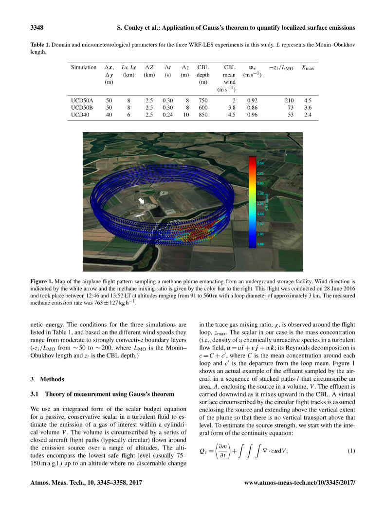
Figure 1. Map of the airplane flight pattern sampling a methane plume emanating from an underground storage facility. Wind direction isindicated by the white arrow and the methane mixing ratio is given by the color bar to the right. This flight was conducted on 28 June 2016and took place between 12:46 and 13:52 LT at altitudes ranging from 91 to 560 m with a loop diameter of approximately 3 km. The measuredmethane emission rate was 763± 127 kg h−1.

netic energy. The conditions for the three simulations arelisted in Table 1, and based on the different wind speeds theyrange from moderate to strongly convective boundary layers(-zi/LMO from ∼ 50 to ∼ 200, where LMO is the Monin–Obukhov length and zi is the CBL depth.)

3 Methods

3.1 Theory of measurement using Gauss’s theorem

We use an integrated form of the scalar budget equationfor a passive, conservative scalar in a turbulent fluid to es-timate the emission of a gas of interest within a cylindri-cal volume V . The volume is circumscribed by a series ofclosed aircraft flight paths (typically circular) flown aroundthe emission source over a range of altitudes. The alti-tudes encompass the lowest safe flight level (usually 75–150 m a.g.l.) up to an altitude where no discernable change

in the trace gas mixing ratio, χ , is observed around the flightloop, zmax. The scalar in our case is the mass concentration(i.e., density of a chemically unreactive species in a turbulentflow field, u= ui+ vj +wk; its Reynolds decomposition isc=C+ c′, where C is the mean concentration around eachloop and c′ is the departure from the loop mean. Figure 1shows an actual example of the effluent sampled by the air-craft in a sequence of stacked paths l that circumscribe anarea, A, enclosing the source in a volume, V . The effluent iscarried downwind as it mixes upward in the CBL. A virtualsurface circumscribed by the circular flight tracks is assumedenclosing the source and extending above the vertical extentof the plume so that there is no vertical transport above thatlevel. To estimate the source strength, we start with the inte-gral form of the continuity equation:

Qc =

⟨∂m

∂t

⟩+

∫ ∫ ∫∇ · cudV, (1)



where 〈〉 denotes an average over the volume V , Qc is thesum of the internal sources and sinks of c within V , and m isthe total mass of c within the volume V . At this point, werecognize that the flux divergence is composed of two terms

∇ · cu= u · ∇c+ c∇ ·u. (2)

In Sect. 3.2 we perform a scale analysis of the terms onthe right-hand side (rhs) of Eq. (2) and show that the sec-ond term, which is proportional to the horizontal wind diver-gence, may be neglected under our normal flight protocol.This is fortunate because of the difficulty in accurately es-timating the horizontal wind divergence from aircraft mea-surements (Lenschow et al., 2007). The vertical flux acrossthe top of the flight cylinder is assumed to be zero, andthe flux from the bottom (ground) is the surface source weare measuring. This leaves us with only the horizontal flux,i.e., cuh, where uh (= ui+ vj ). In order to minimize thecontribution from the horizontal wind divergence term, weremove the loop mean concentration, C, which does not al-ter the first term on the rhs because ∇C= 0, so that Eq. (2)becomes

uh · ∇c+ c∇ ·uh = uh · ∇(c′). (3)

Next, we use Gauss’s theorem to relate the volume integralto a surface integral around the volume that is sampled by theaircraft flight loops:

Qc =

⟨∂m

∂t

⟩+

∫ ∫ ∫∇ · (c′u)dV =

⟨∂m

∂t

⟩+

∫ ∮c′u · n̂dS, (4)

where S is the surface enclosing V and n̂ is an outward point-ing unit vector normal to the surface.

The surface integral can be broken into three elements:a cylinder extending from the ground up to a level abovesignificant modification by the emission, the ground surfacecircumscribed by a low-level (virtual) circular flight path(z= 0), and a nominally horizontal surface circumscribedby a flight path above the level modified by the source(z= zmax). We assume there is no significant flux (other thanthe source of interest) into or out of the ground. Next, thesurface integral is estimated solely from a sequence of closedpath integrals measured by the aircraft at multiple flight lev-els to estimate the right side of Eq. (5) (blue dashed lines inFig. 1),∫ ∮

c′u · n̂dS =

zmax∫0

∮c′uh · n̂dldz, (5)

where l is the flight path.Combining Eqs. (4) and (5) leads to the result that is the

basis for this measurement technique where a series of hor-izontal loops at different altitudes are flown around a sourceregion:

Qc =

⟨∂m

∂t

⟩+

zmax∫0

∮c′uh · n̂dldz. (6)

Along each path the instantaneous outward flux is computedand summed over the loop to yield the mean flux divergencevia Gauss’s theorem. A temporal trend of the total masswithin the volume ( ∂m

∂t) can be estimated from the flight data

and added to the flux divergence integral to obtain the emis-sion rate.

3.2 Divergence uncertainty

In order to estimate the relative error in the horizontal diver-gence term that we are eliminating, we perform a scale analy-sis of the relative size of the two terms in Eq. (2), using sometypical values of the CBL parameters (convective velocityscale w∗= 1 m s−1, boundary layer depth, zi = 1000 m), andsampling geometry (flying at a radius of 1 km around a pointsource.) The Taylor (1922) statistical theory of dispersion ina homogenous and stationary turbulent fluid predicts that theroot mean square lateral (σy) and vertical (σz) dispersion pa-rameters increase linearly with time, or equivalently advec-tion distance, downwind in the near field. Weil (1988) showsseveral examples of the growth of both of these parametersdownwind to be ∼ 0.5w∗, which we use here for a rough es-timate of a conical plume spreading to quantify the dilutionof the source’s emission as it travels downwind to be inter-cepted by the aircraft. We use a large background mixingratio characteristic of global CH4 (∼ 1.9 ppmv), estimate themean gradient by the plume concentration divided by the dis-tance downwind, and assume a conservatively large horizon-tal wind divergence of 10−5 s−1, which may in fact be typicalfor our small sampling region (Stull, 1988). The results areshown in Fig. 2 and, for all but the smallest sources of a fewkilograms per hour and wind speeds below 1 m s−1, the di-vergence term is at least an order of magnitude smaller thanthe gradient term.

3.3 Applying the theory to the LES results

We calculated a comparable estimate of Qc in the LES do-main from the air density, concentration, and wind alongcircular flight paths as a virtual aircraft would fly. Willisand Deardorff (1976) generalized results of their convectiontank experiments to downwind dispersion in the convectiveboundary layer (CBL) in terms of a dimensionless lengthscaleX, the ratio of the horizontal advection time to the largeeddy turnover time:

X =xw∗

Uzi, (7)

where x is the downwind distance and U is the verticallyaveraged mean wind speed.



Figure 2. Graphical representation of the relative magnitude (%)of the contribution of the horizontal wind divergence to the hori-zontal advective terms in Eq. (3), as a function of wind speed andsource magnitude for methane, using a typical global backgroundof 1.9 ppm and divergence of 10−5 s−1.

Figure 3 shows the crosswind-integrated concentrationprofile for the plume release in the UCD50B WRF-LES runas function of X, and normalized height, Z= z/zi . Becauseof the time limitation due to the periodic boundary condi-tions, the plume is averaged for only ∼ 15 min of simula-tion time which is just under a large eddy turnover time forthe conditions of the run. The results displayed in Fig. 3 arein good qualitative agreement with the results of Willis andDeardorff (1976) and Weil et al. (2012), save for the releasebeing at the surface in our LES study, and at Z= 0.067 forthe above studies (see Figs. 1 and 2 of Weil et al., 2012). Fig-ure 3 shows the maximum concentration being lofted nearX∼ 0.2 and leveling off near Z∼ 0.8 around X∼ 0.6; be-yond X> 1.5 the plume is fairly well mixed throughout theextent of the boundary layer.

3.4 The upwind-directed turbulent flux

Horizontal turbulent fluxes are generally ignored in boundarylayer budget studies due to the fact that while they are oftensizeable in magnitude they do not change significantly overhorizontal length scales under consideration (the horizontalhomogeneity assumption). In the vicinity of a point source,however, this is not likely. The method outlined here esti-mates source emissions using a measured horizontal flux thatincorporates wind and scalar measurements at 1 Hz samplerate, resolving scales of ∼ 70 m (Conley et al., 2014), whichshould include nearly all of the turbulent contributions to thehorizontal flux. Here we consider the nature of this turbu-lent flux and the error in emission estimates if only the mean

Figure 3. Relative cross wind integrated concentrations of an efflu-ent plume released at the surface in the UCD50B simulation. Thedata are averaged over 15 min of simulation time and normalized bythe maximum concentration.

transport were considered. We start with the budget equa-tion for a horizontal scalar flux in a horizontally homoge-neous turbulent flow where the molecular diffusive/viscousterm has been neglected (Wyngaard, 2010),

dc′u′

dt=−u′2

∂C

∂x− u′w′

∂C

∂z− c′w′

∂U

∂z−∂c′u′2

∂x

−∂c′u′w′

∂z−

1ρc′∂p′

∂x, (8)

where ρ is density and p′ is the pressure fluctuation. We thenassume stationarity and integrate across the source from apoint just upwind to a point within the plume and obtain

x∫0−

∂c′u′

∂x′dx′ =−

1U

x∫0−

[u′2

∂C

∂x+′+ u′w′

∂C

∂z+ c′w′

∂U

∂z

+∂c′u′2

∂x′+∂c′u′w′

∂z+

1ρc′∂p′

∂x′

]dx′. (9)

We further assume that although the scalar field is not ho-mogeneous the flow field is, and the background horizontalc-flux upwind is much smaller than the flux induced by thepoint source. This results in an equation for the in-plume flux

c′u′ =−1U

u′2 (Cx −Cbckg)+ u′w′

x∫0−

∂C

∂zdx′+

x∫0−

c′w′

∂U

∂z+

x∫0−

(∂c′u′2

∂x′+∂c′u′w′

∂z+

1ρc′∂p′

∂x′

)dx′

.(10)



The first three terms on the rhs of Eq. (10) are negativewithin the plume with their largest magnitudes on the upwindside and diminishing downwind. On the largest, boundary-layer-filling eddy scales, the mean concentration of C down-wind of a source is greater than in the upwind region,(Cx −Cbckg)> 0, and therefore the first term is negative,but decreases in magnitude with distance downwind. How-ever, this term is also positive on smaller scales within theplume where the mean gradient is directed upwind towardsthe source, and is most likely responsible for the speciousintuitive impression that the horizontal turbulent flux shouldtransport the plume downwind from the source along with themean wind advection. Moreover, the second and third termson the rhs are negative because the momentum flux, u′w′, andmean vertical gradient, ∂C/∂z, are negative while the verti-cal turbulent flux, c′w′, and wind shear, ∂U/∂z , are positive.Based on the vertical concentration profiles shown in Weil etal. (2012; their Figs. 3 and 4) it can be inferred that the ver-tical concentration gradient, ∂C/∂z, changes from negativeto positive near X∼ 1 and becomes negligible for X> 2–3.Similarly, in the third term, the vertical flux, c′w′, decreaseswith fetch. Thus the counter-directed flux (c′u′< 0) will fadewith distance downwind. Wyngaard et al. (1971) have shownthat the third-moment, turbulent transport terms (4 and 5 onrhs of Eq. 10) in the horizontal heat flux equation are smallin the surface layer compared to the source terms, so we as-sume the same holds for this scalar flux. Finally, the remain-ing pressure covariance term is believed to be the main sinkin the budget equation working to decorrelate the wind andthe scalar as was shown in the surface layer measurements ofWilczak and Bedard (2004). Therefore, the dominant produc-tion terms for negative c′u′ (terms 1–3 on the rhs of 10) mustbe balanced by the pressure-correlation term leading to anupwind-directed horizontal turbulent flux within the plumethat decreases in magnitude in the downwind direction.

This conclusion is supported by several previous studies.For example, in a wind-tunnel study of flux–gradient rela-tionships, Raupach and Legg (1984) reported that the meanstream-wise horizontal heat flux calculated by multiplyingthe mean wind by the mean temperature overestimates the to-tal heat flux by approximately 10%, which suggests that theturbulent component of the horizontal heat flux is negative;that is, the turbulent flux is upwind, directed counter to themean flow. Other researchers have reported an even largerdisparity. Field experiments by Leuning et al. (1985) indi-cate that the horizontal turbulent flux of a trace gas is∼ 15 %of the mean flux, while Wilson and Shum (1992) suggestit may be 20 %. A recent LES study of particle dispersionover a plant canopy by Pan et al. (2014) indicates magni-tudes of 20 % or more for the negative turbulent componentof scalar fluxes in the vicinity of the source and decreasingwith downwind fetch. We therefore conclude that when sam-pling a near-surface point source at X of order unity or less,if only the mean concentration difference is measured, a sig-nificant overestimate of the scalar source is likely to occur.

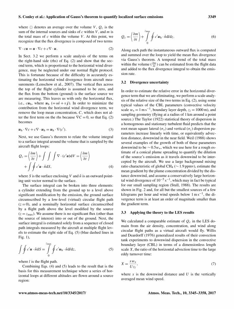
Figure 4. Average cospectrum of the outward-directed compo-nent of the observed wind and the methane concentration from70 laps around a point source near San Antonio, Texas. The peakat 10−2 Hz corresponds to the period of the circle.

Further evidence of this is shown in the average cospec-trum of the outward wind and concentration fluctuation ob-served in the flight loops in Fig. 4. Because the integral of thecospectrum yields the total flux (scalar and wind covariance),this function is useful for examining the contributions to theoverall flux from each of the scales of motion (representedby aircraft speed divided by frequency). The results shown inFig. 4 are from a CH4 point source with an estimated emis-sion rate of 46± 7 kg h−1 which was circled 70 times at adimensionless radius X of approximately 0.35. All cospectraof sampled sources have the same structure seen in Fig. 4:there is an obvious peak at the mean flight loop frequency(usually ∼ 100 s period) followed by a smaller negative dipat higher frequencies within the meandering effluent plume.We believe this to be good evidence that our method cap-tures this important component of the overall flux away fromthe source, which cannot be obtained with a traditional meanwind and an integrated concentration enhancement measure-ment that is so often employed in airborne source estimates(Ryerson et al., 2001; White et al., 1976).

3.5 Choosing the downwind sampling distance

Determining the optimal sampling distance from the targetedpoint source is a balance of several factors. First, not surpris-ingly, the largest plume signal occurs closest to the source(Fig. 3). Second, a high degree of confidence in the resultsis contingent upon sampling the majority of the plume at andabove the lowest flight altitude, which only occurs downwindafter a sufficient time has elapsed to loft the initially near-surface plume. And third, an attempt is made to sample theplume before it reaches the top of the boundary layer so thatthe vertical turbulent entrainment flux does not become ap-preciable violating the assumption of negligible flux throughthe top of the volume V as discussed in Eq. (2). Finally, closeto the source, the fluctuations in concentration will be verylarge, intermittent, at small scales, and highly variable.



Figure 5. Dimensionless flux divergence profiles generated fromaveraging over 3 different WRF-LES runs using 30 time steps foreach one. The horizontal flux per unit altitude (d =F/1z) is nor-malized by the boundary layer height, zi , and source strength, Q.The colored profiles are averages at various dimensionless dis-tances, R= 0.1, 0.2, 0.3, and 0.4, and the gray areas represent 1standard deviation about the mean. The horizontal dashed lines arethe approximate lowest safe flight altitude.

To gain further insight into the second feature of the dis-persing plume, Fig. 5 shows the average horizontal flux di-vergence profiles derived from the three WRF-LES runs.Here we discuss a dimensionless R, which is identical to X,to emphasize that this scaled downwind distance from thesource is a radius of a flight loop. The flux divergence valuesare made dimensionless by the boundary layer height, zi , andthe source emission rate, Q. Very close to the source, beforethe plume has had a chance to loft, the flux divergence profileexhibits a strong gradient below the minimum safe flight alti-tude, making that term difficult to measure directly, as shownin Fig. 5. Farther from the source, the signal becomes weakerwith increasing altitude and eventually becomes increasinglyinfluenced by entrainment fluxes. We therefore seek a sam-pling distance that is far enough to allow sufficient verticallofting yet close enough so that plume crossings are easilyobservable against the background variability and instrumentnoise, and are not yet influenced by entrainment mixing.

Based on the simulation results presented in Fig. 5, we seethe gradient below the lowest flight safe altitude typically be-comes very small for R> 0.4, and therefore we attempt totarget that distance to minimize the extrapolation error fromthe flight data to the surface. We do not currently measure allthe necessary parameters to estimate R in flight (primarilythe surface heat flux (w′θ ′v)0 which is required to estimatew∗). Instead, we estimatew∗ based on the observed boundarylayer height, standard deviation of wind speed, and a param-eterization for w∗= σu/0.6 (Caughey and Palmer, 1979).

Figure 6. Rate of convergence toward the final leak rate estima-tion as a function of the number of loops for LES CASE UCD508.By 15 laps, the emissions estimate (blue line) has stabilized to2.5 kg h−1 compared to the actual leak rate (red line) of 2.9 kg h−1.Dimensionless distance R= 0.25, 50 realizations. Gray area repre-sents 1 SD (standard deviation).

3.6 Minimum number of passes

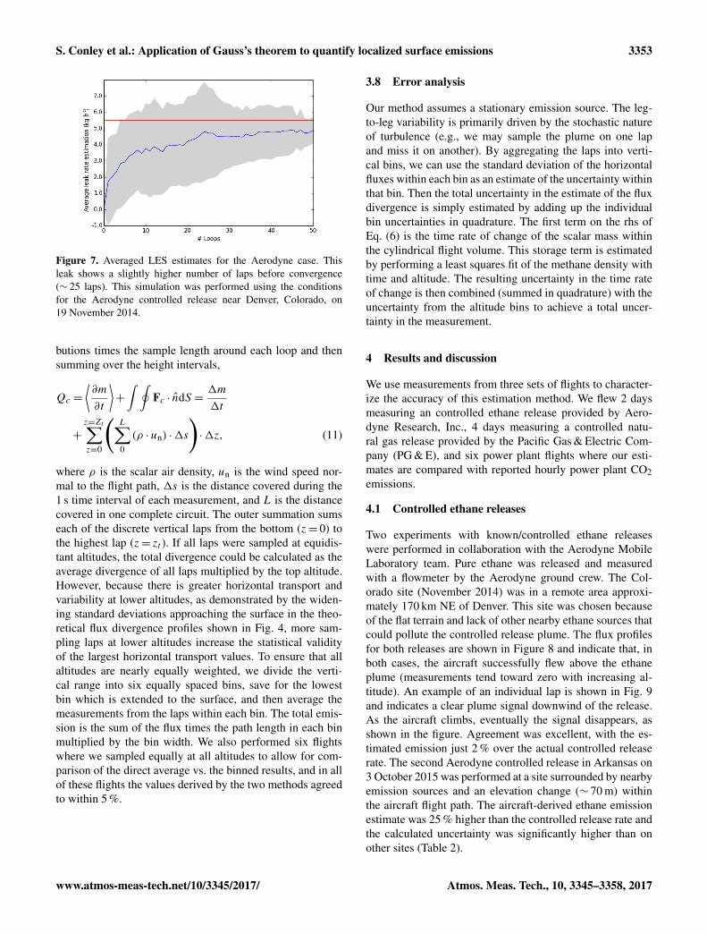
The atmospheric boundary layer is a turbulent medium,meaning that two passes across a plume at the same altitudeand distance downwind will likely make very different mea-surements of the trace gases of interest. A natural questionarises as to how many passes are required to develop a sta-tistically sound estimate of the emission rate. We investigatethe number of passes required to obtain a statistically robustestimate using the WRF-LES results and a controlled releaseexperiment. By calculating the horizontal flux divergenceswith a virtual airplane flying through the simulated tracerfield, and then randomly sampling the flux divergences fromeach of the legs and plotting the resultant estimated emissionrate as a function of the number of samples used, we obtainthe results presented in Fig. 6. The gray region around thered line mean represents the standard deviation of estimatesbased on a random set of loops. Figure 7 shows results froman analysis of actual flight data from the controlled ethane re-lease test near Denver, Colorado, on 19 November 2014. It isevident from both the simulation data and the field data that astatistically stable estimate seems to be achieved somewherebetween 20 and 25 loops around the source.

3.7 Discretization and altitude binning the fluxdivergence data

Measurements of the relevant scalars (e.g., CH4) and mete-orological variables are sampled at discrete time intervals.For our analyses, we interpolate all measurements includ-ing GPS (3 Hz), methane (1 Hz), and temperature (1 Hz), andcomputed variables including horizontal wind (1 Hz), and airdensity (1 Hz) onto a synchronous 1 Hz time series. Next,we estimate the path integral for each individual loop of theflux normal to the flight path by summing up the flux contri-



Figure 7. Averaged LES estimates for the Aerodyne case. Thisleak shows a slightly higher number of laps before convergence(∼ 25 laps). This simulation was performed using the conditionsfor the Aerodyne controlled release near Denver, Colorado, on19 November 2014.

butions times the sample length around each loop and thensumming over the height intervals,

Qc =

⟨∂m

∂t

⟩+

∫ ∮Fc · n̂dS =

1m

1t

+

z=Zt∑z=0

(L∑0(ρ · un) ·1s

)·1z, (11)

where ρ is the scalar air density, un is the wind speed nor-mal to the flight path, 1s is the distance covered during the1 s time interval of each measurement, and L is the distancecovered in one complete circuit. The outer summation sumseach of the discrete vertical laps from the bottom (z= 0) tothe highest lap (z= zt ). If all laps were sampled at equidis-tant altitudes, the total divergence could be calculated as theaverage divergence of all laps multiplied by the top altitude.However, because there is greater horizontal transport andvariability at lower altitudes, as demonstrated by the widen-ing standard deviations approaching the surface in the theo-retical flux divergence profiles shown in Fig. 4, more sam-pling laps at lower altitudes increase the statistical validityof the largest horizontal transport values. To ensure that allaltitudes are nearly equally weighted, we divide the verti-cal range into six equally spaced bins, save for the lowestbin which is extended to the surface, and then average themeasurements from the laps within each bin. The total emis-sion is the sum of the flux times the path length in each binmultiplied by the bin width. We also performed six flightswhere we sampled equally at all altitudes to allow for com-parison of the direct average vs. the binned results, and in allof these flights the values derived by the two methods agreedto within 5 %.

3.8 Error analysis

Our method assumes a stationary emission source. The leg-to-leg variability is primarily driven by the stochastic natureof turbulence (e.g., we may sample the plume on one lapand miss it on another). By aggregating the laps into verti-cal bins, we can use the standard deviation of the horizontalfluxes within each bin as an estimate of the uncertainty withinthat bin. Then the total uncertainty in the estimate of the fluxdivergence is simply estimated by adding up the individualbin uncertainties in quadrature. The first term on the rhs ofEq. (6) is the time rate of change of the scalar mass withinthe cylindrical flight volume. This storage term is estimatedby performing a least squares fit of the methane density withtime and altitude. The resulting uncertainty in the time rateof change is then combined (summed in quadrature) with theuncertainty from the altitude bins to achieve a total uncer-tainty in the measurement.

4 Results and discussion

We use measurements from three sets of flights to character-ize the accuracy of this estimation method. We flew 2 daysmeasuring an controlled ethane release provided by Aero-dyne Research, Inc., 4 days measuring a controlled natu-ral gas release provided by the Pacific Gas & Electric Com-pany (PG & E), and six power plant flights where our esti-mates are compared with reported hourly power plant CO2emissions.

4.1 Controlled ethane releases

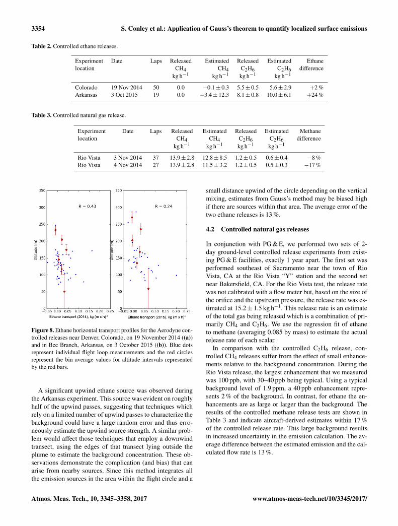
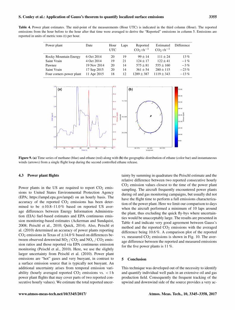
Two experiments with known/controlled ethane releaseswere performed in collaboration with the Aerodyne MobileLaboratory team. Pure ethane was released and measuredwith a flowmeter by the Aerodyne ground crew. The Col-orado site (November 2014) was in a remote area approxi-mately 170 km NE of Denver. This site was chosen becauseof the flat terrain and lack of other nearby ethane sources thatcould pollute the controlled release plume. The flux profilesfor both releases are shown in Figure 8 and indicate that, inboth cases, the aircraft successfully flew above the ethaneplume (measurements tend toward zero with increasing al-titude). An example of an individual lap is shown in Fig. 9and indicates a clear plume signal downwind of the release.As the aircraft climbs, eventually the signal disappears, asshown in the figure. Agreement was excellent, with the es-timated emission just 2 % over the actual controlled releaserate. The second Aerodyne controlled release in Arkansas on3 October 2015 was performed at a site surrounded by nearbyemission sources and an elevation change (∼ 70 m) withinthe aircraft flight path. The aircraft-derived ethane emissionestimate was 25 % higher than the controlled release rate andthe calculated uncertainty was significantly higher than onother sites (Table 2).



Table 2. Controlled ethane releases.

Experiment Date Laps Released Estimated Released Estimated Ethanelocation CH4 CH4 C2H6 C2H6 difference

kg h−1 kg h−1 kg h−1 kg h−1

Colorado 19 Nov 2014 50 0.0 −0.1± 0.3 5.5± 0.5 5.6± 2.9 +2 %Arkansas 3 Oct 2015 19 0.0 −3.4± 12.3 8.1± 0.8 10.0± 6.1 +24 %

Table 3. Controlled natural gas release.

Experiment Date Laps Released Estimated Released Estimated Methanelocation CH4 CH4 C2H6 C2H6 difference

kg h−1 kg h−1 kg h−1 kg h−1

Rio Vista 3 Nov 2014 37 13.9± 2.8 12.8± 8.5 1.2± 0.5 0.6± 0.4 −8 %Rio Vista 4 Nov 2014 27 13.9± 2.8 11.5± 3.2 1.2± 0.5 0.5± 0.3 −17 %

Figure 8. Ethane horizontal transport profiles for the Aerodyne con-trolled releases near Denver, Colorado, on 19 November 2014 ((a))and in Bee Branch, Arkansas, on 3 October 2015 ((b)). Blue dotsrepresent individual flight loop measurements and the red circlesrepresent the bin average values for altitude intervals representedby the red bars.

A significant upwind ethane source was observed duringthe Arkansas experiment. This source was evident on roughlyhalf of the upwind passes, suggesting that techniques whichrely on a limited number of upwind passes to characterize thebackground could have a large random error and thus erro-neously estimate the upwind source strength. A similar prob-lem would affect those techniques that employ a downwindtransect, using the edges of that transect lying outside theplume to estimate the background concentration. These ob-servations demonstrate the complication (and bias) that canarise from nearby sources. Since this method integrates allthe emission sources in the area within the flight circle and a

small distance upwind of the circle depending on the verticalmixing, estimates from Gauss’s method may be biased highif there are sources within that area. The average error of thetwo ethane releases is 13 %.

4.2 Controlled natural gas releases

In conjunction with PG & E, we performed two sets of 2-day ground-level controlled release experiments from exist-ing PG & E facilities, exactly 1 year apart. The first set wasperformed southeast of Sacramento near the town of RioVista, CA at the Rio Vista “Y” station and the second setnear Bakersfield, CA. For the Rio Vista test, the release ratewas not calibrated with a flow meter but, based on the size ofthe orifice and the upstream pressure, the release rate was es-timated at 15.2± 1.5 kg h−1. This release rate is an estimateof the total gas being released which is a combination of pri-marily CH4 and C2H6. We use the regression fit of ethaneto methane (averaging 0.085 by mass) to estimate the actualrelease rate of each scalar.

In comparison with the controlled C2H6 release, con-trolled CH4 releases suffer from the effect of small enhance-ments relative to the background concentration. During theRio Vista release, the largest enhancement that we measuredwas 100 ppb, with 30–40 ppb being typical. Using a typicalbackground level of 1.9 ppm, a 40 ppb enhancement repre-sents 2 % of the background. In contrast, for ethane the en-hancements are as large or larger than the background. Theresults of the controlled methane release tests are shown inTable 3 and indicate aircraft-derived estimates within 17 %of the controlled release rate. This large background resultsin increased uncertainty in the emission calculation. The av-erage difference between the estimated emission and the cal-culated flow rate is 13 %.



Table 4. Power plant estimates. The mid-point of the measurements (Hour UTC) is indicated in the third column (Hour). The reportedemissions from the hour before to the hour after that time were averaged to derive the “Reported” emissions in column 5. Emissions arereported in units of metric tons (t) per hour.

Power plant Date Hour Laps Reported Estimated DifferenceUTC CO2 t h−1 CO2 t h−1

Rocky Mountain Energy 6 Oct 2014 20 19 99± 14 111± 24 13 %Saint Vrain 4 Oct 2014 19 21 124± 17 122± 41 −1 %Pawnee 19 Nov 2014 20 14 575± 81 555± 160 −3 %Saint Vrain 17 Sep 2015 20 14 361± 54 280± 115 −23 %Four corners power plant 11 Apr 2015 18 12 1289± 387 1119± 343 −13 %

Figure 9. (a) Time series of methane (blue) and ethane (red) along with (b) the geographic distribution of ethane (color bar) and instantaneouswinds (arrows) from a single flight loop during the second controlled ethane release.

4.3 Power plant flights

Power plants in the US are required to report CO2 emis-sions to United States Environmental Protection Agency(EPA; https://ampd.epa.gov/ampd) on an hourly basis. Theaccuracy of the reported CO2 emissions has been deter-mined to be ±10.8–11.0 % based on reported US aver-age differences between Energy Information Administra-tion (EIA) fuel-based estimates and EPA continuous emis-sion monitoring-based estimates (Ackerman and Sundquist,2008; Peischl et al., 2010; Quick, 2014). Also, Peischl etal. (2010) determined an accuracy of power plants reportingCO2 emissions in Texas of±14.0 % based on differences be-tween observed downwind SO2 /CO2 and NOx /CO2 emis-sion ratios and those reported via EPA continuous emissionmonitoring (Peischl et al., 2010). Here, we use the slightlylarger uncertainty from Peischl et al. (2010). Power plantemissions are “hot” gases and very buoyant, in contrast toa surface emission source that is typically not buoyant. Anadditional uncertainty arises from temporal emission vari-ability (hourly averaged reported CO2 emissions vs. < 1 hpower plant flights that may cover parts of two reported con-secutive hourly values). We estimate the total reported uncer-

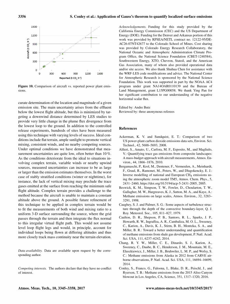
tainty by summing in quadrature the Peischl estimate and therelative difference between two reported consecutive hourlyCO2 emission values closest to the time of the power plantsampling. The aircraft frequently encountered power plantsduring oil and gas monitoring campaigns, but usually did nothave the flight time to perform a full emissions characteriza-tion of the power plant. Here we limit our comparison to dayswhen the aircraft performed a minimum of 10 laps aroundthe plant, thus excluding the quick fly-bys where uncertain-ties would be unacceptably large. The results are presented inTable 4 and indicate very good agreement between Gauss’smethod and the reported CO2 emissions with the averageddifference being 10.6 %. A comparison plot of the reportedvs. measured CO2 emissions is shown in Fig. 10. The aver-age difference between the reported and measured emissionsfor the five power plants is 11 %.

5 Conclusion

This technique was developed out of the necessity to identifyand quantify individual well pads in an extensive oil and gasproduction field. Consequently the frequent tracking of theupwind and downwind side of the source provides a very ac-


https://ampd.epa.gov/ampd


Figure 10. Comparison of aircraft vs. reported power plant emis-sions.

curate determination of the location and magnitude of a givenemission site. The main uncertainty arises from the effluentbelow the lowest flight altitude, but this is minimized by tar-geting a downwind distance determined by LES studies toprovide very little change in the plume flux divergence fromthe lowest loop to the ground. In addition to the controlledrelease experiments, hundreds of sites have been measuredusing this technique with varying levels of success. Ideal con-ditions include flat terrain, ample sunlight to promote verticalmixing, consistent winds, and no nearby competing sources.Under optimal conditions we have demonstrated that mea-surement uncertainties are quite low, often better than 10 %.As the conditions deteriorate from the ideal to situations in-volving complex terrain, variable winds or nearby upwindsources, measured uncertainties can increase to be as largeor larger than the emission estimates themselves. In the worstcase of stably stratified conditions (winter or nighttime), forinstance, the lack of vertical mixing may preclude the tracegases emitted at the surface from reaching the minimum safeflight altitude. Complex terrain provides a challenge to themethod because the aircraft is unable to maintain a constantaltitude above the ground. A possible future refinement ofthis technique to be applied in complex terrain would beto fit the measurements of both wind and mixing ratio to auniform 3-D surface surrounding the source, where the gridpasses through the terrain and then integrate the flux normalto this irregular virtual flight path. This would not assumelevel loop flight legs and would, in principle, account forindividual loops being flown at differing altitudes and thusmore closely track mass continuity near the terrain elevation.

Data availability. Data are available upon request by the corre-sponding author.

Competing interests. The authors declare that they have no conflictof interest.

Acknowledgements. Funding for this study provided by theCalifornia Energy Commission (CEC) and the US Department ofEnergy (DOE). Funding for the Denver and Arkansas portion of thiswork was provided by RPSEA/NETL contract no. 12122-95/DE-AC26-07NT42677 to the Colorado School of Mines. Cost sharingwas provided by Colorado Energy Research Collaboratory, theNational Oceanic and Atmospheric Administration Climate Pro-gram Office, the National Science Foundation (CBET-1240584),Southwestern Energy, XTO, Chevron, Statoil, and the AmericanGas Association, many of whom also provided operational dataand/or site access. We also thank Shuhua Chen for assistance withthe WRF-LES code modifications and advice. The National Centerfor Atmospheric Research is sponsored by the National ScienceFoundation. This work was supported in part by the NOAA AC4program under grant NA14OAR0110139 and the Bureau ofLand Management, grant L15PG00058. We thank Ying Pan forher significant contribution to our understanding of the negativehorizontal scalar flux.

Edited by: Andre ButzReviewed by: three anonymous referees

References

Ackerman, K. V. and Sundquist, E. T.: Comparison of twoUS power-plant carbon dioxide emissions data sets, Environ. Sci.Technol., 42, 5688–5693, 2008.

Alfieri, S., Amato, U., Carfora, M. F., Esposito, M., and Magliulo,V.: Quantifying trace gas emissions from composite landscapes:A mass-budget approach with aircraft measurements, Atmos. En-viron., 44, 1866–1876, 2010.

Bergamaschi, P., Krol, M., Dentener, F., Vermeulen, A., Meinhardt,F., Graul, R., Ramonet, M., Peters, W., and Dlugokencky, E. J.:Inverse modelling of national and European CH4 emissions us-ing the atmospheric zoom model TM5, Atmos. Chem. Phys., 5,2431–2460, https://doi.org/10.5194/acp-5-2431-2005, 2005.

Beswick, K. M., Simpson, T. W., Fowler, D., Choularton, T. W.,Gallagher, M. W., Hargreaves, K. J., Sutton, M. A., and Kaye, A.:Methane emissions on large scales, Atmos. Environ., 32, 3283–3291, 1998.

Caughey, S. J. and Palmer, S. G.: Some aspects of turbulence struc-ture through the depth of the convective boundary-layer, Q. J.Roy. Meteorol. Soc., 105, 811–827, 1979.

Caulton, D. R., Shepson, P. B., Santoro, R. L., Sparks, J. P.,Howarth, R. W., Ingraffea, A. R., Cambaliza, M. O. L., Sweeney,C., Karion, A., Davis, K. J., Stirm, B. H., Montzka, S. A., andMiller, B. R.: Toward a better understanding and quantificationof methane emissions from shale gas development, P. Natl. Acad.Sci. USA, 111, 6237–6242, 2014.

Chang, R. Y. W., Miller, C. E., Dinardo, S. J., Karion, A.,Sweeney, C., Daube, B. C., Henderson, J. M., Mountain, M. E.,Eluszkiewicz, J., Miller, J. B., Bruhwiler, L. M. P., and Wofsy, S.C.: Methane emissions from Alaska in 2012 from CARVE air-borne observations, P. Natl. Acad. Sci. USA, 111, 16694–16699,2014.

Conley, S., Franco, G., Faloona, I., Blake, D. R., Peischl, J., andRyerson, T. B.: Methane emissions from the 2015 Aliso Canyonblowout in Los Angeles, CA, Science, 351, 1317–1320, 2016.


https://doi.org/10.5194/acp-5-2431-2005


Conley, S. A., Faloona, I. C., Lenschow, D. H., Karion, A., andSweeney, C.: A Low-Cost System for Measuring HorizontalWinds from Single-Engine Aircraft, J. Atmos. Ocean. Tech., 31,1312–1320, 2014.

Crosson, E. R.: A cavity ring-down analyzer for measuring atmo-spheric levels of methane, carbon dioxide, and water vapor, Appl.Phys. B, 92, 403–408, 2008.

Czepiel, P. M., Mosher, B., Harriss, R. C., Shorter, J. H., McManus,J. B., Kolb, C. E., Allwine, E., and Lamb, B. K.: Landfill methaneemissions measured by enclosure and atmospheric tracer meth-ods, J. Geophys. Res.-Atmos., 101, 16711–16719, 1996.

Denmead, O. T., Harper, L. A., Freney, J. R., Griffith, D. W. T., Le-uning, R., and Sharpe, R. R.: A mass balance method for non-intrusive measurements of surface-air trace gas exchange, At-mos. Environ., 32, 3679–3688, 1998.

Gallagher, M. W., Choularton, T. W., Bower, K. N., Stromberg, I.M., Beswick, K. M., Fowler, D., and Hargreaves, K. J.: Measure-ments of methane fluxes on the landscape scale form a wetlandarea in North Scotland, Atmos. Environ., 28, 2421–2430, 1994.

Gerbig, C., Lin, J. C., Wofsy, S. C., Daube, B. C., Andrews, A.E., Stephens, B. B., Bakwin, P. S., and Grainger, C. A.: Towardconstraining regional-scale fluxes of CO2 with atmospheric ob-servations over a continent: 2. Analysis of COBRA data usinga receptor-oriented framework, J. Geophys. Res.-Atmos., 108,4756, https://doi.org/10.1029/2002JD003018, 2003.

Gordon, M., Li, S.-M., Staebler, R., Darlington, A., Hayden, K.,O’Brien, J., and Wolde, M.: Determining air pollutant emissionrates based on mass balance using airborne measurement dataover the Alberta oil sands operations, Atmos. Meas. Tech., 8,3745–3765, https://doi.org/10.5194/amt-8-3745-2015, 2015.

Hacker, J. M., Chen, D. L., Bai, M., Ewenz, C., Junkermann, W.,Lieff, W., McManus, B., Neininger, B., Sun, J. L., Coates, T.,Denmead, T., Flesch, T., McGinn, S., and Hill, J.: Using airbornetechnology to quantify and apportion emissions of CH4 and NH3from feedlots, Animal Prod. Sci., 56, 190–203, 2016.

Hiller, R. V., Neininger, B., Brunner, D., Gerbig, C., Bretscher, D.,Kunzle, T., Buchmann, N., and Eugster, W.: Aircraft-based CH4flux estimates for validation of emissions from an agriculturallydominated area in Switzerland, J. Geophys. Res.-Atmos., 119,4874–4887, 2014.

Hirsch, A. I., Michalak, A. M., Bruhwiler, L. M., Peters,W., Dlugokencky, E. J., and Tans, P. P.: Inverse mod-eling estimates of the global nitrous oxide surface fluxfrom 1998–2001, Global Biogeochem. Cy., 20, GB1008,https://doi.org/10.1029/2004GB002443, 2006.

Kalthoff, N., Corsmeier, U., Schmidt, K., Kottmeier, C., Fiedler, F.,Habram, M., and Slemr, F.: Emissions of the city of Augsburgdetermined using the mass balance method, Atmos. Environ., 36,S19–S31, 2002.

Karion, A., Sweeney, C., Petron, G., Frost, G., Hardesty, R. M.,Kofler, J., Miller, B. R., Newberger, T., Wolter, S., Banta, R.,Brewer, A., Dlugokencky, E., Lang, P., Montzka, S. A., Schnell,R., Tans, P., Trainer, M., Zamora, R., and Conley, S.: Methaneemissions estimate from airborne measurements over a westernUnited States natural gas field, Geophys. Res. Lett., 40, 4393–4397, 2013.

Karion, A., Sweeney, C., Kort, E. A., Shepson, P. B., Brewer, A.,Cambaliza, M., Conley, S. A., Davis, K., Deng, A. J., Hardesty,M., Herndon, S. C., Lauvaux, T., Lavoie, T., Lyon, D., New-

berger, T., Petron, G., Rella, C., Smith, M., Wolter, S., Yacov-itch, T. I., and Tans, P.: Aircraft-Based Estimate of Total MethaneEmissions from the Barnett Shale Region, Environ. Sci. Technol.,49, 8124–8131, 2015.

Lamb, B. K., McManus, J. B., Shorter, J. H., Kolb, C. E., Mosher,B., Harriss, R. C., Allwine, E., Blaha, D., Howard, T., Guenther,A., Lott, R. A., Siverson, R., Westberg, H., and Zimmerman, P.:Development of atmospheric tracer methods to measure methaneemissions form natural-gas facilities and urban areas, Environ.Sci. Technol., 29, 1468–1479, 1995.

Lavoie, T. N., Shepson, P. B., Cambaliza, M. O. L., Stirm, B. H.,Karion, A., Sweeney, C., Yacovitch, T. I., Herndon, S. C., Lan,X., and Lyon, D.: Aircraft-Based Measurements of Point SourceMethane Emissions in the Barnett Shale Basin, Environ. Sci.Technol., 49, 7904–7913, 2015.

Lenschow, D. H., Savic-Jovcic, V., and Stevens, B.: Divergenceand vorticity from aircraft air motion measurements, J. Atmos.Ocean. Tech., 24, 2062–2072, 2007.

Leuning, R., Freney, J. R., Denmead, O. T., and Simpson, J. R.: Asampler for measuring atmospheric ammonia flux, Atmos. Envi-ron., 19, 1117–1124, 1985.

Mays, K. L., Shepson, P. B., Stirm, B. H., Karion, A., Sweeney, C.,and Gurney, K. R.: Aircraft-Based Measurements of the CarbonFootprint of Indianapolis, Environ. Sci. Technol., 43, 7816–7823,2009.

Miller, J. B., Lehman, S. J., Montzka, S. A., Sweeney, C., Miller,B. R., Karion, A., Wolak, C., Dlugokencky, E. J., Southon,J., Turnbull, J. C., and Tans, P. P.: Linking emissions of fos-sil fuel CO2 and other anthropogenic trace gases using atmo-spheric (CO2)-C-14, J. Geophys. Res.-Atmos., 117, D08302,https://doi.org/10.1029/2011JD017048, 2012.

Miller, S. M., Wofsy, S. C., Michalak, A. M., Kort, E. A., Andrews,A. E., Biraud, S. C., Dlugokencky, E. J., Eluszkiewicz, J., Fis-cher, M. L., Janssens-Maenhout, G., Miller, B. R., Miller, J. B.,Montzka, S. A., Nehrkorn, T., and Sweeney, C.: Anthropogenicemissions of methane in the United States, P. Natl. Acad. Sci.USA, 110, 20018–20022, 2013.

Muhle, S., Balsam, I., and Cheeseman, C. R.: Comparison of carbonemissions associated with municipal solid waste management inGermany and the UK, Resour. Conserv. Recycl., 54, 793–801,2010.

Neef, L., van Weele, M., and van Velthoven, P.: Optimal estimationof the present-day global methane budget, Global Biogeochem.Cy., 24, GB4024, https://doi.org/10.1029/2009GB003661, 2010.

Nisbet, E. and Weiss, R.: Top-Down Versus Bottom-Up, Science,328, 1241–1243, 2010.

Pan, Y., Chamecki, M., and Isard, S. A.: Large-eddy simulation ofturbulence and particle dispersion inside the canopy roughnesssublayer, J. Fluid Mech., 753, 499–534, 2014.

Peischl, J., Ryerson, T. B., Holloway, J. S., Parrish, D. D.,Trainer, M., Frost, G. J., Aikin, K. C., Brown, S. S., Dube,W. P., Stark, H., and Fehsenfeld, F. C.: A top-down analy-sis of emissions from selected Texas power plants during Tex-AQS 2000 and 2006, J. Geophys. Res.-Atmos., 115, D16303,https://doi.org/10.1029/2009JD013527, 2010.

Peischl, J., Ryerson, T. B., Brioude, J., Aikin, K. C., Andrews, A. E.,Atlas, E., Blake, D., Daube, B. C., de Gouw, J. A., Dlugokencky,E., Frost, G. J., Gentner, D. R., Gilman, J. B., Goldstein, A. H.,Harley, R. A., Holloway, J. S., Kofler, J., Kuster, W. C., Lang,


https://doi.org/10.1029/2002JD003018

https://doi.org/10.5194/amt-8-3745-2015

https://doi.org/10.1029/2004GB002443

https://doi.org/10.1029/2011JD017048

https://doi.org/10.1029/2009GB003661

https://doi.org/10.1029/2009JD013527


P. M., Novelli, P. C., Santoni, G. W., Trainer, M., Wofsy, S. C.,and Parrish, D. D.: Quantifying sources of methane using lightalkanes in the Los Angeles basin, California, J. Geophys. Res.-Atmos., 118, 4974-4990, 2013.

Petron, G., Karion, A., Sweeney, C., Miller, B. R., Montzka, S.A., Frost, G. J., Trainer, M., Tans, P., Andrews, A., Kofler,J., Helmig, D., Guenther, D., Dlugokencky, E., Lang, P., New-berger, T., Wolter, S., Hall, B., Novelli, P., Brewer, A., Conley,S., Hardesty, M., Banta, R., White, A., Noone, D., Wolfe, D.,and Schnell, R.: A new look at methane and nonmethane hydro-carbon emissions from oil and natural gas operations in the Col-orado Denver-Julesburg Basin, J. Geophys. Res.-Atmos., 119,6836–6852, 2014.

Quick, J. C.: Carbon dioxide emission tallies for 210 U.S. coal-firedpower plants: A comparison of two accounting methods, J. AirWaste Manage. Assoc., 64, 73–79, 2014.

Raupach, M. R. and Legg, B. J.: The uses and limitations of flux–gradient relationships in micrometeorology, Agr. Water Manage.,8, 119–131, 1984.

Ritter, J. A., Barrick, J. D. W., Watson, C. E., Sachse, G. W., Gre-gory, G. L., Anderson, B. E., Woerner, M. A., and Collins, J. E.:Airborne boundary-layer flux measurements of trace species overCanadian boreal forest and northern wetland regions, J. Geophys.Res.-Atmos., 99, 1671–1685, 1994.

Roscioli, J. R., Yacovitch, T. I., Floerchinger, C., Mitchell, A.L., Tkacik, D. S., Subramanian, R., Martinez, D. M., Vaughn,T. L., Williams, L., Zimmerle, D., Robinson, A. L., Hern-don, S. C., and Marchese, A. J.: Measurements of methaneemissions from natural gas gathering facilities and processingplants: measurement methods, Atmos. Meas. Tech., 8, 2017–2035, https://doi.org/10.5194/amt-8-2017-2015, 2015.

Ryerson, T. B., Buhr, M. P., Frost, G. J., Goldan, P. D., Holloway, J.S., Hubler, G., Jobson, B. T., Kuster, W. C., McKeen, S. A., Par-rish, D. D., Roberts, J. M., Sueper, D. T., Trainer, M., Williams,J., and Fehsenfeld, F. C.: Emissions lifetimes and ozone for-mation in power plant plumes, J. Geophys. Res.-Atmos., 103,22569–22583, 1998.

Ryerson, T. B., Trainer, M., Holloway, J. S., Parrish, D. D., Huey,L. G., Sueper, D. T., Frost, G. J., Donnelly, S. G., Schauffler, S.,Atlas, E. L., Kuster, W. C., Goldan, P. D., Hubler, G., Meagher,J. F., and Fehsenfeld, F. C.: Observations of ozone formation inpower plant plumes and implications for ozone control strategies,Science, 292, 719–723, 2001.

Stull, R. B.: An Introduction to Boundary Layer Meteorology,Kluwer Academic Publishers, Norwell, MA, 1988.

Taylor, G. I.: Diffusion by Continuous Movements, Proc. Lond.Math. Soc., s2-20, 196–212, 1922.

Tratt, D. M., Buckland, K. N., Hall, J. L., Johnson, P. D., Keim,E. R., Leifer, I., Westberg, K., and Young, S. J.: Airborne visu-alization and quantification of discrete methane sources in theenvironment, Remote Sensing Environ., 154, 74–88, 2014.

Turnbull, J. C., Karion, A., Fischer, M. L., Faloona, I., Guilder-son, T., Lehman, S. J., Miller, B. R., Miller, J. B., Montzka, S.,Sherwood, T., Saripalli, S., Sweeney, C., and Tans, P. P.: Assess-ment of fossil fuel carbon dioxide and other anthropogenic tracegas emissions from airborne measurements over Sacramento,California in spring 2009, Atmos. Chem. Phys., 11, 705–721,https://doi.org/10.5194/acp-11-705-2011, 2011.

Wecht, K. J., Jacob, D. J., Frankenberg, C., Jiang, Z., and Blake,D. R.: Mapping of North American methane emissions with highspatial resolution by inversion of SCIAMACHY satellite data, J.Geophys. Res.-Atmos., 119, 7741–7756, 2014.

Weil, J. C.: Dispersion in the Convective Boundary Layer, in: Lec-tures on Air Pollution Modeling, edited by: Venkatram, A. andWyngaard, J. C., American Meteorological Society, Boston, MA,1988.

Weil, J. C., Sullivan, P. P., Patton, E. G., and Moeng, C.-H.: Statisti-cal Variability of Dispersion in the Convective Boundary Layer:Ensembles of Simulations and Observations, Bound.-Lay. Mete-orol., 145, 185–210, 2012.

White, W. H., Anderson, J. A., Blumenthal, D. L., Husar, R. B.,Gillani, N. V., Husar, J. D., and Wilson Jr., W. E.: Formation andTransport of Secondary Air Pollutants: Ozone and Aerosols inthe St. Louis Urban Plume, Science, 194, 187–189, 1976.

Wilczak, J. M. and Bedard, A. J.: A new turbulence microbarome-ter and its evaluation using the budget of horizontal heat flux, J.Atmos. Ocean. Tech., 21, 1170–1181, 2004.

Willis, G. E. and Deardorff, J. W.: Laboratory model of diffusioninto convective planetary bounday-layer, Q. J. Roy. Meteorol.Soc., 102, 427–445, 1976.

Wilson, J. D. and Shum, W. K. N.: A reexamination of the integratedhorizontal flux method of estimating volatilization from circularplots, Agr. Forest Meteorol., 57, 281–295, 1992.

Wratt, D. S., Gimson, N. R., Brailsford, G. W., Lassey, K. R., Brom-ley, A. M., and Bell, M. J.: Estimating regional methane emis-sions from agriculture using aircraft measurements of concentra-tion profiles, Atmos. Environ., 35, 497–508, 2001.

Wyngaard, J. C.: Turbulence in the Atmosphere, Cambridge Uni-versity Press, Cambridge, 2010.

Wyngaard, J. C. , Coté, O. R., and Izumi, Y.: Local free convection,similarity, and the budgets of shear stress and heat flux, J. Atmos.Sci., 28, 1171–1182, 1971.

Yacovitch, T. I., Herndon, S. C., Roscioli, J. R., Floerchinger, C.,McGovern, R. M., Agnese, M., Petron, G., Kofler, J., Sweeney,C., Karion, A., Conley, S. A., Kort, E. A., Nahle, L., Fischer, M.,Hildebrandt, L., Koeth, J., McManus, J. B., Nelson, D. D., Zah-niser, M. S., and Kolb, C. E.: Demonstration of an Ethane Spec-trometer for Methane Source Identification, Environ. Sci. Tech-nol., 48, 8028–8034, 2014.

Yuan, B., Kaser, L., Karl, T., Graus, M., Peischl, J., Campos, T. L.,Shertz, S., Apel, E. C., Hornbrook, R. S., Hills, A., Gilman, J. B.,Lerner, B. M., Warneke, C., Flocke, F. M., Ryerson, T. B., Guen-ther, A. B., and de Gouw, J. A.: Airborne flux measurements ofmethane and volatile organic compounds over the Haynesvilleand Marcellus shale gas production regions, J. Geophys. Res.-Atmos., 120, 6271–6289, 2015.


https://doi.org/10.5194/amt-8-2017-2015

https://doi.org/10.5194/acp-11-705-2011

Application of Gauss's theorem to quantify localized surface ...

Documents

Transcript of Application of Gauss's theorem to quantify localized surface ...