A Species-Conserving Genetic Algorithm for Multimodal Optimization

A Species-Conserving Genetic Algorithm for Multimodal Optimization

by

Michael Scott Brown

A dissertation submitted in partial fulfillment of the requirements for the degree of Doctor of Philosophy

in Computer Science

Graduate School of Computer and Information Sciences Nova Southeastern University

2010

UMI Number: 3433233

All rights reserved

INFORMATION TO ALL USERS The quality of this reproduction is dependent upon the quality of the copy submitted.

In the unlikely event that the author did not send a complete manuscript

and there are missing pages, these will be noted. Also, if material had to be removed, a note will indicate the deletion.

UMI 3433233

Copyright 2011 by ProQuest LLC. All rights reserved. This edition of the work is protected against

unauthorized copying under Title 17, United States Code.

ProQuest LLC 789 East Eisenhower Parkway

P.O. Box 1346 Ann Arbor, MI 48106-1346

We hereby certify that this dissertation, submitted by Michael Scott Brown, conforms to acceptable standards and is fully adequate in scope and quality to fulfill the dissertation requirements for the degree of Doctor of Philosophy. _____________________________________________ ________________ Michael Laszlo, Ph.D. Date Chairperson of Dissertation Committee _____________________________________________ ________________ James Cannady, Ph.D. Date Dissertation Committee Member _____________________________________________ ________________ Sumitra Mukherjee, Ph.D. Date Dissertation Committee Member Approved: _____________________________________________ ________________ Leonidas Irakliotis, Ph.D. Date Dean

Graduate School of Computer and Information Sciences Nova Southeastern University

2010

An Abstract of a Dissertation Submitted to Nova Southeastern University in Partial Fulfillment of the Requirements for the Degree of Doctor of Philosophy

A Species-Conserving Genetic Algorithm for Multimodal Optimization

by

Michael Scott Brown

September 2010

The problem of multimodal functional optimization has been addressed by much research producing many different search techniques. Niche Genetic Algorithms is one area that has attempted to solve this problem. Many Niche Genetic Algorithms use some type of radius. When multiple optima occur within the radius, these algorithms have a difficult time locating them. Problems that have arbitrarily close optima create a greater problem. This paper presents a new Niche Genetic Algorithm framework called Dynamic-radius Species-conserving Genetic Algorithm. This new framework extends existing Genetic Algorithm research. This new framework enhances an existing Niche Genetic Algorithm in two ways. As the name implies the radius of the algorithm varies during execution. A uniform radius can cause issues if it is not set correctly during initialization. A dynamic radius compensates for these issues. The framework does not attempt to locate all of the optima in a single pass. It attempts to find some optima and then uses a tabu list to exclude those areas of the domain for future iterations. To exclude these previously located optima, the framework uses a fitness sharing approach and a seed exclusion approach. This new framework addresses many areas of difficulty in current multimodal functional optimization research. This research used the experimental research methodology. A series of classic benchmark functional optimization problems were used to compare this framework to other algorithms. These other algorithms represented classic and current Niche Genetic Algorithms. Results from this research show that this new framework does very well in locating optima in a variety of benchmark functions. In functions that have arbitrarily close optima, the framework outperforms other algorithms. Compared to other Niche Genetic Algorithms the framework does equally well in locating optima that are not arbitrarily close. Results indicate that varying the radius during execution and the use of a tabu list assists in solving functional optimization problems for continuous functions that have arbitrarily close optima.

Acknowledgments

I would like to thank Dr. Laszlo for being my dissertation chair. His help cannot be overstated. I would also like to thank Dr. Cannady and Dr. Mukherjee for serving on my committee. I would also like to thank my parents, Thomas and Sandra Brown. You always told me that I could do anything if I only worked hard and never gave up. You were right. This dissertation is dedicated to the three ladies in my life, Truocmai Dinh, Jessica Maikhanh Brown and Tiffany Maitam Brown, my wife and two daughters. All that I do, I do for you.

v

Table of Contents

Abstract iii List of Tables vii List of Figures ix Chapters

1. Introduction 1 Problem Statement 1 Research Goal 3 Approach 5 Relevance and Significance 8 Barriers and Issues 9 Definition of Terms 12 Summary 14 2. Review of the Literature 16

Relevant Research Other than NGAs 16 Fitness Sharing Methods 18 Crowding Methods 24 Other Niche Genetic Algorithm Methods 36

Summary 48 3. Methodology 49 Research Method Employed 49 Specific Procedures Employed 50 Format for Presenting Results 66 Resources Required 67 Summary 67

4. Results 69

Parameter Settings and Implementation Methods 69 Results of Algorithms on F1 77 Results of Algorithms on F2 79 Results of Algorithms on F3 80 Results of Algorithms on F4 81 Results of Algorithms on F5 82 Results of Algorithms on F6 84 Results of Algorithms on F7 85 Results of Algorithms on F8 87 Summary of Results 88

5. Conclusions, Implications, Recommendations and Summary 90

Conclusions 90 Implications 93

vi

Recommendations 94 Summary 95

Appendixes A. Ranking of Algorithms 102

Reference List 110

vii

List of Tables

Tables 1. Tabu Search Decision 17

2. Sequential Niche Technique Algorithm 22

3. Genetic Algorithm with Species Algorithm 28

4. Species Conserving Genetic Algorithm Seed Selection 30

5. Species Conserving Genetic Algorithm Species Conservation 31

6. Crowding Clustering Genetic Algorithm 34

7. Enhanced Evolutionary Tabu Search Algorithm 39

8. Genetic Algorithm and Particle Swarm Optimization Algorithm 41

9. Cellular Genetic Algorithm 42

10. DSGA Parameters 51

11. DSGA Algorithm 52

12. DSGA Algorithm Initialization 53

13. Seed Selection 54

14. Seed Conservation for each Generation 55

15. Test Functions 60

16. Benchmark Algorithm Comparison 64

17. Fitness Functions 73

18. Results for Equation F1 78




viii





26. Ranking of Algorithms 102

ix

List of Figures

Figures 1. Graph of y = x sin (x2) 2 2. Graph of f(x) = 4 (x – 0.5)2 26 3. Graph of f(x) = 2.8 (x - 0.6)2 26 4. Chart of Recall and Precision for F1 78 5. Chart of Recall and Precision for F2 80 6. Chart of Recall and Precision for F3 81 7. Chart of Recall and Precision for F4 82 8. Chart of Recall and Precision for F5 83 9. Chart of Recall and Precision for F6 85 10. Chart of Recall for F7 85 11. Chart of Recall and Precision for F8 88

1

Chapter 1

Introduction

This introductory chapter is organized into seven sections. The first section defines

the problem that this research addressed. The second section describes the research goal.

The third section provides an overview of the approach. The fourth section explains the

relevance and significance. The fifth section describes the barriers and issues that need to

be overcome by this research. The sixth section provides definitions of terms used in the

dissertation. The final section is a summary of this chapter.

Problem Statement

Genetic Algorithms (GA) have a difficult time solving problems with multiple correct

answers. When traditional GAs attempt to solve multimodal problems they often

converge to only one of the possible correct or good solutions. A current area of research

in GAs is called Niche Genetic Algorithms (NGA), which hopes to address this problem.

NGAs can be used to solve problems that seek local optima where multiple exist.

Currently there are many NGAs. Two prominent approaches to developing NGAs are

crowding and sharing (Deb & Goldberg, 1989). In crowding algorithms, members of one

population coexist with members of the next population. Older individuals of the

population are selected for removal based on how similar they are to newer members. A

variety of NGAs use some type of crowding scheme (Cavicchio, 1970; De Jong, 1975;

Jelasity & Dombi 1998; Li, Balazs, Parks & Clarkson, 2002; Ling, Wa, Yang & Wang,

2

2008; Raghuwanshi & Kakde, 2007). The second approach is through fitness sharing. In

sharing schemes, the fitness of an individual is dependent on its distance to other

individuals in the population. This increases the chance that species will form around

niches by rewarding genetic isolation. There are many methods based on sharing

schemes (Beasley, Bull & Martin, 1993b; Bernier, 1996; Goldberg & Richardson, 1987;

Holland, 1975). While not every NGA is a crowding or sharing method, most fall into

one of these two categories.

Figure 1. Graph of y = x sin(x2)

Both of these approaches use some form of distance in determining what individuals

perform crossover or which individuals are promoted into the next generation. There are

some domains where distance is not a good indicator of niches (Ando & Kobayashi,

2005). Clearly these approaches are good if there are significant distances between

niches. What is unclear is the effectiveness of these approaches when niches become

3

arbitrarily close. Consider functional optimization problems for continuous functions,

specifically, classes of functions that have local optima that become arbitrarily close. No

matter what distance a NGA expects between niches there exists an area in the domain in

which niches are smaller than this distance. Figure 1 shows a graph of one such function,

y = x sin(x2). As x gets larger the local maximums or optima become arbitrarily close

together.

Research Goal

The goal of this research was to develop a new NGA that can address these types of

problems for functional optimization of continuous functions. This NGA is a framework

based on an existing NGA, but allows different components to be used in combination to

create different algorithms. This new approach is not dependent on a static niche radius

parameter that could provide poor results if selected wrong. As part of this goal the

algorithm should be flexible enough to solve other types of problems that current

traditional NGAs solve. This research goal will expand our current understanding of

NGAs.

This dissertation addressed of few areas that make up the goal. To accomplish the

goal a new NGA was developed and tested against existing NGAs. The areas that this

research addressed are as follows:

• To develop a new NGA that will solve for arbitrarily close optima

• To compare this new NGA to existing NGAs to determine its effectiveness

These two research goals complement the goals defined in this chapter.

4

There were two hypotheses to this research. The first hypothesis was that locating

optima in phases increases a NGAs ability to find optima. In the first phase the NGA

finds some optima. Once some optima are located, they are used to encourage

exploration in other areas of the domain. Multiple attempts to find optima are performed.

Each attempt leverages already located optima, which should make it easier to locate

other optima because there is less of the domain space to search. This process continues

until all of the optima are located.

The second hypothesis was that many NGAs miss optima, especially arbitrarily close

optima, because they use a static radius. Many current NGAs have a parameter that is

used to determine if individuals are within a neighborhood. If the distance between

optima is smaller than this radius, the NGA has a difficult time locating all of the optima.

The value that this parameter is set to greatly affects the results of the NGA. The second

hypothesis was that a dynamic radius could compensate for poor radius choices.

Allowing the radius to change as the algorithm runs may allow it to adapt to conditions

and find more optima.

These two hypotheses complement each other. The research hypothesis was that

better results can be obtained by allowing dynamic radius and restricting areas of the

domain where optima have been located. This allows investigation across the entire

domain which should produce better results. Both hypotheses should increase the

number of optima discovered by the NGA.

5

Approach

The new approach for solving multimodal optimization problems used existing

methods in combination to enhance a traditional GA. The new approach is a NGA

framework that is based on Species Conserving Genetic Algorithm (SCGA) (Li et al.,

2002). The framework is presented in a modular form and has different components that

can be used in combination to create different variations of the algorithm.

SCGA enhances the traditional GA with seed selection and seed conservation steps.

Seeds are identified as the fittest member within a given radius. Seeds are conserved into

the next generation through a seed conservation step. Seed conservation has the seed

replace the weakest individual in the new generation within the radius of the seed. This

ensures that these strong individuals that are tracking different optima are preserved.

The new framework does not attempt to find all of the optima within a single pass of

the algorithm. Traditional GAs perform a loop with each iteration creating a new

generation of the population. Environmental pressures force the population to converge.

Multimodal optimization creates a difficult problem for GAs. The new approach

generates a certain number of generations in hopes of finding some optima. These

optima are recorded and the environmental parameters change. These changes alter how

the fitness of individuals is determined and what individuals can be seeds. This

encourages future generations to avoid these optima. This allows future generations to

explore other areas of the domain and locate other optima. The process of locating some

optima and then changing the fitness is performed multiple times. There is an outer loop

and an inner nested loop. The inner loop performs a typical SCGA algorithm. Once it

6

completes, seeds and optima are recorded and changes are made to the algorithm

parameters. The steps consisting of the inner loop, recording and changing of the

algorithm’s parameters are performed in an outer loop. While traditional GAs are a

single loop, this new approach uses nested loops to find some of the optima that enhances

its ability to locate all of the optima.

The new framework also changes the radius used to define species. In SCGA a radius

is defined and used throughout the algorithm. As other research has shown there is a

limitation to algorithms of this type (Ando & Kobayashi, 2005). Poor choices for the

radius produce poor results. The new approach changes the radius as the algorithm runs.

The algorithm attempts to compensate for poor radius choices. After each inner loop of

the algorithm completes, adjustments are made to the radius. Varying the radius

mitigates the issue of incorrectly set radius.

The final difference between SCGA and this new framework is the use of a tabu list.

A tabu list comes from the tabu search method and is a list that contains previously

evaluated areas of the domain. The tabu list is used by the algorithm to avoid these areas

in the future and concentrate on areas of the domain that have not been searched. After

each completion of the inner loop, the seeds and optima from that pass are recorded on a

tabu list. This list is used in future loops of the algorithm to encourage exploration by

avoiding these areas.

As optima are located, the algorithm adjusts to encourage exploration into other areas

of the domain. This is done in two ways. The algorithm can determine that a potential

individual is too close to a member of the tabu list. This will disqualify the individual

from becoming a seed. The algorithm may also adjust the fitness to individuals relative

7

to how close they are to individuals on the tabu list. This will decrease their chances of

becoming seeds. Both of these tactics are possible within the new framework.

To validate the new approach, it was compared against other NGAs using a set of well

established benchmarks. The benchmarks came from a variety of NGA research. All of

the benchmarks were minimization and maximization functional optimization problems.

A new benchmark was also presented. These benchmarks were used to compare the new

approach to other NGAs.

The new approach was compared to other NGAs in solving the benchmarks that were

defined. A variety of performance criteria were used in this comparison including

proportions of peaks located and average fitness of the last 50 generations. For each

benchmark the new approach was compared to multiple other NGAs. These other NGAs

had been selected to cover a wide range of NGA research from modern methods to early

algorithms. In many cases the new approach was compared against previously published

results in other NGA research. In other cases NGAs were implemented to obtain test

results. The performance criteria allowed the new approached to be evaluated against

other NGA methods.

The new framework leveraged a variety of existing methods to introduce a new

combination of concepts to create a NGA framework. The use of a tabu list in a NGA

has been used before (McLoughlin & Cedeno, 2005; Ting & Ko, 2008; Tsai, Tseng,

Chiang, & Yang, 2009). The use of a dynamic radius has also been used in other

algorithms (Jelasity & Dombi, 1998). The combination of a tabu list and dynamic radius

applied to the SCGA algorithm is new. This new framework was compared against other

NGAs using well defined benchmarks and criteria. Comparing it against many well

8

established NGAs showed that this new approach can solve multimodal optimization

problems.

Relevance and Significance

The study of GAs is important because GAs are very useful search techniques. They

have been used in almost every field of study. Much literature has been dedicated to

outlining uses for GAs (Coello, 2000; Dianati, Song & Treiber, 2002; Sheikh,

Raghuwanshi & Jaiswal, 2008). For example, GAs and NGAs have been used in

Electrical Engineering to design electromagnetic systems (Cioffi, Formisano & Martone,

2000). In the field of Knowledge Discovery they have been used as a classifier (Pozo &

Hasse, 2000). For pattern matching, NGAs can be used to match handwriting (Oliveira,

Sabourin, Bortolozzi & Suen, 2002; Stefano, Cioppa & Marcelli, 1999). NGA research is

useful to many fields of study.

Because GAs and NGAs are applicable to many fields of study, research in the subject

has continued uninterrupted for many decades. Early researchers developed simple

algorithms for multimodal optimization (Deb & Goldberg, 1989; Goldberg &

Richardson, 1987; Mauldin, 1984). These algorithms solved many multimodal

optimization problems. A second generation of algorithms were developed that

addressed limitations of the previous algorithms (Li et al., 2002; Ling et al., 2008;

Raghuwanshi & Kakde, 2007). Some research addressed the limitation that many

algorithms require tuning parameters (Bernier, 1995; Fonseca & Fleming, 1993).

Researchers continue to investigate NGAs.

9

NGA research continues to this day and is an important area of research in Artificial

Intelligence. Experts in the field believe that developing new NGAs is useful and

justification exists for continued investigation. These new NGAs can be used in other

areas of research to solve multimodal optimization and search problems.

Barriers and Issues

There were two barriers to this research. The first barrier was premature convergence

which traditional GAs exhibit when attempting to locate multiple optimum. The second

barrier was optimum location and preservation. Let us consider how each of these areas

was addressed by this research.

Premature Convergence

One barrier to developing a NGA is to prevent global convergence. A GA naturally

converges to a local optimum. This is appropriate for many types of problems, but there

are problems that have multiple optima. Traditional GAs will converge to a single

optimum, ignoring the other ones. The key to develop a NGA is to overcome this

pressure to converge. The NGA needs to allow local convergence within niches. De

Jong (1975) calls this premature convergence.

Two forces act on the generations of a traditional GA. Crossover of individuals puts

pressure on the population to converge through different individuals having different

probabilities of reproducing (De Jong, 1975). The algorithm exploits fit individuals in

the creation of each generation. An opposite force works against this exploitation.

Mutation alters individuals, which allow exploration of new areas of the domain

10

(Beasley, Bull & Martin, 1993a). NGAs need to balance the two forces of exploration

and exploitation. Too much exploration will decrease the performance of the search,

turning it into a random search (Holland, 1992). Limiting exploration too much, in favor

of exploitation, leads to premature convergence (De Jong, 1975). Successful NGAs

balance exploration and exploitation to locate multiple optima.

As a GA generates individuals using crossover, the amount of the domain that is being

searched decreases. This is referred to as genetic drift and removes areas of the search

space so greatly that even mutation cannot put them back (De Jong, 1975). This

eliminates other possible solutions to the problem. In problems that have a single correct

answer this convergence helps in solving the problem by eliminating areas of the domain

in which the correct answer does not exist. But in multi-objective problems, it eliminates

other optima.

There are two methods in GA research that could address this problem. One is to have

a very large population size N. If N is very large, the GA has much more time to locate

other optima before the genetic drift closes the search space. However, this leads to

performance problems (De Jong, 1975). A second approach is to have a very high

mutation rate. This would allow the expanding of the search space when genetic drift

happens. The problem with very high mutation rates is that it prevents convergence,

which is the ultimate goal of the GA and the way that the GA finds the solution (De Jong,

1975). This is why De Jong, Holland, Goldberg and other researchers believe that

traditional GAs will not solve multimodal problems (De Jong, 1975; Holland, 1975;

Goldberg & Richardson, 1987).

11

Optimum Preservation

The second barrier to this research was optimum preservation. This barrier can be

thought of in two parts. The first part is optimum location, identifying the areas of the

domain worth preserving. Because the domain has not fully been searched when

optimum location is applied, this is difficult for the NGAs. The second part is how to

preserve or conserve these areas. Because of crossover and mutation, there is little

guarantee that these areas of interest will be represented in the next generation. Optimum

preservation is essential in NGAs.

Optimum location attempts to identify individuals within a population that can

eventually lead to an optimum (De Jong, 1975). These individuals are normally

individuals at, or close to, an optimum. Selection in traditional GAs focuses on the fittest

members. But in multimodal optimization problems, it is possible that less fit members

are also tracking a local optimum. A single generation of a population represents a very

small part of the domain. Locating these individuals makes optimum location

challenging.

Optimum preservation is used to ensure that the optima located are not eliminated in

the population through convergence. Convergence pressures of GAs can eliminate

optimum after they are discovered. The method to ensure that an optimum is preserved

can be direct or subtle (Li et al., 2002). There are direct approaches like promoting an

individual of interest into the next generation. More subtle approaches can be to adjust

the individual's fitness to increase its chances of being selected for crossover. Regardless

of the method, these located optimum need to be preserved into the next generation.

12

Optimum preservation is a barrier that every successful NGA needs to overcome.

Some part of the algorithm needs to identify interesting individuals in the population and

allow their representation in future generations (Li et al., 2002). There are a variety of

methods that can be employed for optimum preservation. These methods will be

described in the literature review of Chapter 2.

Definition of Terms

This dissertation uses a variety of terms. Many terms are generally known in the GA

field. The following list of terms should provide an overview of terms used in this

dissertation.

Baldwin Effect: The Baldwin Effect is a biological theory that the fitness of an

individual can be changed by environmental factors (Baldwin, 1896).

Cluster: A cluster is a set of items that share something in common. Within a cluster

items should have commonality and items in different clusters should have differences

(Sheikh, Raghuwanshi & Jaiswal, 2008).

Convergence: Convergence is a process in which new generations of a population

have decreased genetic diversity. This typically occurs around an optimum.

Crossover: Crossover is a genetic operation that takes two individuals of a population

and by interchanging genes between the two individuals creates two new individuals.

Evolutionary Algorithms: Evolutionary algorithms are a classification of algorithms

based upon natural evolution. There are four subclasses of evolutionary algorithms:

13

Evolutionary Programming, Evolutionary Strategies, Genetic Algorithms and Genetic

Programming (Dianati, Song & Treiber, 2002).

Fitness: Fitness is a measurement assigned to an individual of a population that

relates to how well the individual copes with environmental pressure (De Jong, 1975).

Genetic Algorithm: A Genetic Algorithm is a specific type of search method that was

developed by Bremermann (1958). The algorithm models the domain as a series of gene

values. An initial generation of the population is created, normally randomly, of different

combinations of these gene values. Genetic operations are applied to the generation to

create a new generation. Over time the population converges to the optimum of the

domain.

Genetic Drift: Genetic Drift is the change in probability or frequency that a certain

gene value appears in a population (De Jong, 1975). As populations evolve certain gene

values become more prevalent.

Inversion: Inversion is a genetic operation in which the ordering of the genes change

(Holland, 1975).

Mutation: Mutation is a genetic operation in which a gene value is randomly changed

based upon the mutation rate.

Niche Genetic Algorithm: A Niche Genetic Algorithm is a specific type of Genetic

Algorithm that promotes genetic diversity (Mahfoud, 1995).

Pareto Front: The Pareto Front is the set of non-dominant optimal values for a multi-

objective optimization problem (Alba, Dorronsoro, Luna, Nebro & Bouvry, 2005).

Particle Swarm Optimization: Particle Swarm Optimization is a specific search

technique that simulates swarm intelligence.

14

Premature Convergence: Premature convergence is when a Genetic Algorithm

converges at such a rate that optima are removed from the search space (De Jong, 1975).

Seed: A Seed is a dominant individual within a certain area of the domain in a

population (Li et al., 2002).

Selection: Selection is a process of selecting individuals of a population to reproduce.

Species: The term species has different definitions in NGA research. In this research

the Li et al. (2002) definition will be used. Species are individuals within a population,

whose distance is less than some, pre-define parameter (Li et al., 2002).

This section contains definitions of terms used in this dissertation.

Summary

This research had a few specific goals. The research produced a new NGA

framework. This framework allows for the creation of multiple variations of the NGA

algorithm. The problem that the new NGA addresses is functional optimization for

continuous functions. Within this area, the goal is to solve for functions that have

arbitrarily close optima. These types of functions are especially difficult for NGAs. A

secondary goal was for the algorithm to solve other types of optimization problems

equally well as other NGAs. The new NGA framework was developed to accomplish

these goals.

The approach that was taken created a new NGA framework that applies existing

techniques to NGA research. The NGA uses multiple passes in an effort to locate some

optima and uses those optima in locating the other ones. The algorithm varies the radius

15

used in determining seeds. A tabu list is used to store located optima and seeds, so these

areas of the domain are not revisited.

16

Chapter 2

Review of the Literature

This literature review covers the history and current state of NGA research. It is

organized into five sections. The first section describes research that is relevant to this

research, but that is not an NGA. NGA research is organized in the next three sections.

There are sharing methods, crowding methods and a section for methods that do not fall

into either of these groups. Finally, there is a summary section.

Relevant Research Other than NGAs

The framework presented in this paper leverages many other concepts in existing

NGA research. However, some concepts of the framework come from other research

areas. This section provides a literature review of other research that was influential in

developing this framework.

Tabu Search

The new algorithm presented in this paper uses aspects of the tabu search. A tabu

search is an optimization technique used to avoid local optima (Glover, 1989; Glover,

1990a). It has been used to solve several optimization problems (Glover, 1990b; Hansen,

1997). The tabu search has an associated memory structure that is used to store previous

moves in the optimization process. This list is used to prevent the algorithm from

returning to previously obtained optima.

17

A tabu search begins with a possible solution to the optimization problem. Each

iteration of the algorithm will apply an operation that will move from one solution state

to a new one. Table 1 shows the part of the tabu search algorithm that determines if a

move should be made.

Table 1. Tabu Search Decision Line Number Pseudocode

1 Select a move 2 If the move is on the tabu list then 3 If the move satisfies the aspiration condition 4 Make the move 5 Else 6 Select another move 7 Else 8 Make the move

The operation is added to the tabu list. Future iterations of the algorithm prevent the

operation from being applied, unless an aspiration condition is met. The aspiration

condition determines if the move is superior to the current solution. By using the tabu list,

the tabu search avoids local optima and locates the optimal solution to the problem.

The tabu search uses a short-term memory structure to track previous moves (Glover,

1990b). This memory structure is used to prevent the algorithm from revisiting

previously visited states. The tabu list can be finite or infinite in length. A finite tabu list

only stores a certain number of previous moves. When the list is full the oldest move will

be removed when a new move is added. The algorithm prevents these moves from being

made in the future. If the tabu list is finite, then the move can only be made after the

previous move is purged from the tabu list. The tabu list encourages exploration.

The aspiration condition is used in a tabu search to override the tabu list (Glover,

1990b). If a move is on the tabu list, it is normally prohibited. But before the potential

18

move is eliminated, it is compared to an aspiration condition. If the move meets the

aspiration condition, the move is performed. This allows superior moves from being

eliminated because they are tabu.

The tabu search is a useful search technique. Previous research has shown that

combining the tabu search with evolutionary algorithms can increase its accuracy. Tabu

searches have been combined with GAs (McLoughlin & Cedeno, 2005; Ting & Ko,

2008; Tsai, et al., 2009). They have also been combined with Evolutionary Programming

algorithms (Rajan & Mohan, 2004). The tabu search can provide valuable insight into

solving multimodal optimization problems.

Fitness Sharing Methods

A common approach to solving multimodal optimization problems is through fitness

sharing. While methods for fitness sharing vary, they all alter the fitness function in

some way to encourage genetic diversity. In multimodal functional optimization

problems, fitness is normally directly related to the objective function. In Sharing

Methods distance to other individuals is incorporated into the fitness function to

encourage exploration. This prevents a single optimum from dominating the population.

Some of the earliest approaches for NGA algorithms are sharing methods.

Holland, J. H.

Holland (1975) provides a formal framework for GA research. While it does not

provide a specific NGA algorithm, it does describe some of the earlier fitness sharing

concepts. Holland describes a two-armed bandit to represent the problem that can be

19

solved by NGAs. A two-armed bandit is a slot machine that has two handles, instead of

one. Each handle has a different payout. Players may elect to pull the left or right

handle. Ideally, every player would select to pull the handle with the highest payout, but

there is a catch. For a given turn all of the players that select a given handle must share

the payout. With this new rule the problem is not obvious which handle the players

should select. Each handle is a niche and by dividing the payout, or fitness, between all

individuals within a niche allows the GA to solve the problem. By defining the fitness

function in such a way as to reflect other individuals in the niche, allows a traditional GA

to solve for multimodal optimization problems. This is some of the earliest research in

fitness sharing.

Goldberg and Richardson

Another seminal work in NGA is Goldberg and Richardson (1987). This NGA

introduces a sharing function. In traditional GAs fitness functions determine the

probability a member of a population will reproduce. In a multimodal problem once a

traditional GA discovers a niche, it converges on it, ignoring other possible niches. A

sharing function is used to reduce this convergence by using the shared fitness to

determine the probability that a member will reproduce. Shared fitness penalizes

individuals that are close to other individuals in the population and rewards isolated

individuals. This allows the NGA to locate other niches.

In the Goldberg and Richardson (1987) method the algorithm is the same as a

traditional GA, except for determining the fitness function. The algorithm uses a shared

fitness function that accepts the distance between two members as an input parameter.

20

These functions must conform to three properties. The function's output must be between

zero and one. When the distance is zero, the output must be one. When the distance

approaches infinity, the output must be zero. When shared fitness is computed for

individual p, a niche count is calculated by summing the sharing function of all the other

members of the population with respect to p. The shared fitness is the individual’s raw

fitness divided by the niche count.

While the Goldberg and Richardson (1987) fitness sharing algorithm can take many

forms, their research presents an example of the algorithm. The example attempts to

locate the five local optima of the function f(x) = sin6 (5.1 π x + 0.5), where x is between

0 and 1. The shared fitness function selected was the power law function, which is

shown below.

sh(d) = { =

α

−

shareó1

d

if d < σshare

= 0 otherwise

The parameters σshare and α are set to 0.1 and 1 respectively. The niche count, mi, for

individual i is represented by the following function.

mi = )),((

1ji

N

jxxdsh

=Σ

In the niche count xi is individual i and xj spans all individuals in the population N. The

shared fitness of an individual is simply fi’ = fi / mi, where fi’ is the shared fitness, fi is the

raw fitness and mi is the niche count. The research results showed that traditional GAs

only found one optima of the function. The sharing fitness algorithm found all five

21

optima and had an equal number of individuals at each optimum (Goldberg &

Richardson, 1987).

Sequential Niche Technique

The Sequential Niche Technique (SNT) is a search technique that can be applied to a

GA (Beasley, Bull & Martin, 1993b). It attempts to locate one optimum at a time. Once

an optimum is located the technique adjusts the search algorithm to locate another

optimum. The technique is successful because it reduces the search problem into locating

a single optimum.

When applying SNT to a GA, the traditional steps of a GA are used. The fitness

function, which typically is the objective function, is modified. This modified fitness

function is used in the algorithm. After the algorithm runs, the best individual is recorded

on a list. The modified fitness function is changed by adding a derating function for the

fittest individual that was located. The derating function can take many forms, but its

affect is to decrease the fitness around the located individual. This excludes this area of

the domain as a place for likely optima. Future runs of the GA seek out other optima.

SNT also has a solution threshold. If the fittest individual after each run is more fit than

the solution threshold, it is considered an optimum. The algorithm for SNT is shown in

Table 2.

SNT allows search algorithms to use previous knowledge about the problem to

simplify it. This approach is attributed to other functional optimization research (Ackley,

1987). It is a useful technique that allows search algorithms to take complex problems

22

like multimodal functional optimization and break them into a series of much simpler

problems of single functional optimization.

Table 2. Sequential Niche Technique Algorithm Line

Number Pseudocode

1 Assign modified fitness function to objective function 2 While not termination condition 3 Run traditional GA using modified fitness function 4 After GA runs record the optimum that it finds 5 Depress optimum area in the modified fitness function 6 If optimum in step 4 is larger than solution threshold,

display it as a solution 7 End loop

Bernier’s BDM and BPM

The Bernier (1996) method uses a Minimum Spanning Tree (MST) for fitness sharing.

It is used in each iteration of the NGA to adjust the fitness of individuals. There are two

algorithms for the method: Biggest Different Method (BDM) and Biggest Proportion

Method (BPM). BDM and BPM use Prim’s MST algorithm although any MST

algorithm might be used.

The Prim’s MST algorithm is used to determine a tree, T, with minimum total weight

from a graph, G. Graphs have vertices, V, and edges, E, that connect two vertices. Every

edge has an associated weight, W. Because an edge connects two vertices, we can

represent it as (u, v) where u and v are vertices. Prim’s algorithm begins by randomly

selecting a vertex for the tree T. Then it computes the weight from every vertex in T to

every vertex not in T and selects the one with the minimum weight. The selected vertex

and associated edge are added to T. Prim grows the minimum tree, starting with a single

vertex, into a MST.

23

Bernier adapts MST to GAs. Individuals are represented by vertices. The weight of

the edge between two individuals is defined as their Euclidean distance. Bernier’s

hypothesis is that by removing some number of the largest edges of the MST, what is left

will be trees around each niche. Bernier offers two methods to determine what edges

should be removed. The BDM looks at the longest 15% of the edges in the MST. It sorts

these edges in descending order according to their weight, w(e1), w(e2) … w(en). The

algorithm computes the weight difference between consecutive edges, so ∆1 = w(e1) –

w( e2), ∆2 = w(e2) – w(e3),, … ∆(n-1) = w(e(n-1)) – w(en). Finally the algorithm locates the

largest ∆, ∆x. All of the edges, w(e1) through w(ex) are removed leaving x +1 trees.

Each tree corresponds to a niche. The BPM is very similar to the BDM. Instead of

comparing differences between edges, it compares proportions. The top 15% of edges

are sorted in descending order. Proportions are computed by dividing consecutive edges,

p1 = w(e1) /w( e2), p2 = w(e2) / w(e3),, … p(n-1) = w(e(n-1)) / w(en). The edges with the

largest proportion are removed. BDM and BPM adjust the fitness of the individuals

around niches using standard fitness sharing techniques.

Results from Bernier’s algorithm are very impressive. In six benchmark functions

BDM and BPM located nearly 90% of the optima. A goal of this research was to develop

a NGA that does not need parameters. What is unclear is how the MST parameter of

15% affects the final results. It would seem that if there were more optima than 15% of

the number of individuals in the population, this algorithm would have difficulties. If

there were more optima than 15% of the population, then some optima would not have

their fitness adjusted through fitness sharing. Another case could be a situation where

there were relatively few optima but a very large population size. Considering so many

24

edges could lead the algorithm into forming too many niches. Perhaps this percentage

should be a parameter.

Fitness Sharing Summary

This section describes many fitness sharing NGAs. Some very important concepts

come out of fitness sharing methods. All of the algorithms use the idea of altering the

fitness function to guide the direction that the next generation will take. SNT introduces

a concept of locating a single optimum and then using the fitness function to exclude it in

future generations. Fitness sharing is a useful technique to encourage exploration across

the domain space.

Crowding Methods

Crowding methods are another common approach to developing NGAs. Crowding

methods replace members of one generation with members of a previous generation

based upon their similarity. They promote genetically diverse individuals and encourage

exploration across the domain space. A variety of crowding methods have been

successful with multimodal functional optimization problems.

Cavicchio

Cavicchio’s (1970) research looks at selection schemes to solve multimodal

optimization problems. This research is some of the earliest work in the NGA area.

Cavicchio introduces a series of selection schemes. In Cavicchio’s NGA a certain

number of the fittest individuals are carried over into the next generation. The number of

25

individuals carried over into the next generation is a parameter of the algorithm.

Offspring also have to compete to be placed into the next generation.

Cavicchio (1970) introduces three Preselection Schemes. The first scheme is based on

an observation that many offspring are fit enough to be placed into the next generation,

but not more fit then their parents. Allowing this seems to be counterproductive. So, the

first scheme requires offspring to be more fit than both of their parents to be introduced

into the next generation. The second scheme enhances the first scheme, but adds the

requirement that the worst parent is to be removed from the population. The third

scheme only requires an offspring to be more fit than one of its parents. Preselection is

one of the earliest forms of NGAs.

Because of hardware limitations of the 1970s, tests on Cavicchio’s algorithm were

limited to very few individuals. In many cases population sizes were between 10 and 20

individuals (Cavicchio, 1970). Little research has been published with benchmarks on

Cavicchio’s NGA since the original research. It is difficult to determine how this NGA

would perform with more modern benchmarks.

De Jong

Some of the earliest works to address the problem of GAs converging globally even

on multimodal domains were from De Jong (1975) and Holland (1975). De Jong's Elitist

Model R2 introduces the strategy of including the best members of one generation in the

next generation. After each generation is created, its least fit members are replaced by an

equal number of the fittest members of the previous generation. The Elitist Model R2

replaces only one member from the previous population, but this idea can be expanded to

26

some predetermined fixed number of individuals. This influence can be seen in later

NGAs (Li et al., 2002).

Figure 2. Graph of f(x) = 4(x – 0.5)2

It is easy to see why an elitist strategy would work for domains that have equally fit

optima. Consider the equation f(x) = 4(x – 0.5)2, where 0 <= x <= 1 as shown in Figure

2. Here there are two optima of equal fitness. A traditional GA will converge to one

optimum or the other, but not both. An elitist strategy would preserve individuals of both

optima. If considering an equation like f(x) = 2.8(x – 0.6)2, where 0 <= x <= 1, elitist

strategies seem less useful. This equation is shown in Figure 3. Here there are two local

optima, x = 0 and x = 1. However, x = 1 is a local, but not global optimum.

Figure 3. Graph of f(x) = 2.8(x – 0.6)2

27

An elitist strategy will probably not preserve individuals near the x = 1 local optimum.

These equations come from Goldberg and Richardson (1987).

Another NGA method described by De Jong (1975) is the Crowding Factor Model R5.

The Crowding Factor Model R5 simulates an environment in which parents and offspring

live together. To keep the population size stable, the system allows certain parents to die.

This is done in crowded areas of the domain. In this method populations overlap one

another. The Crowding Factor R5 method uses two parameters. Generation gap is the

proportion of a population that is produced each generation. In De Jong's example it was

0.1, which means that the NGA produces enough individuals to increase the population

size by 10% each generation. The second parameter is the crowding factor. For each

new member of the population, an old member must be removed. The crowding factor is

the number of old members considered for removal for each new member. In De Jong's

example it was three. This NGA will randomly evaluate three old members for each new

member. Of the three old members the one that is genetically similar to the new member

is removed.

Genetic Algorithm with Species

Genetic Algorithm with Species (GAS) extends the crowding method concept by

defining species (Jelasity & Dombi, 1998). Species are groups of individuals that are

tracking a common optimum. Like other crowding methods GAS only allows crossover

with individuals within the same species. This algorithm allows the population size to

expand and contract for each generation. It also introduces the concept of individuals

dying off. Traditional GAs have a generation die when the next generation is created.

28

GAS allows fit individuals to live longer than weak ones by allowing them to be

members of multiple generations.

In GAS a species is defined as the triplet (o, l, S) (Jelasity & Dombi, 1998). The

variable S is the population that makes up the species and o is the individual with the

maximum fitness within the species. GAS uses a decreasing radius. The equation, R,

defines the radius values as it decreases. R must always be greater than the maximum

distance between two individuals and should approach 0. There is an index associated

with the various radii, called the radius index. In the species l is the radius index when

the species was defined. The radius for a given triplet (o, l, S) is R(l).

The algorithm shown in Table 3 outlines the steps that GAS uses to create a new

generation (Jelasity & Dombi, 1998). T is the current population and MP is a parameter

that determines how large T can become. MP is not the size of T, rather the upper limit to

the size of T. The algorithm for generation T will loop until the size of T is greater than

MP. Within the loop two parents are selected, p1 and p2. They produce two offspring,

o1 and o2. Parents and offspring are put back into the population.

Table 3. Genetic Algorithm with Species Algorithm Line

Number Pseudocode

1 While (population size of T < MP) 2 Select two parents, p1 and p2 within the

same (o, l, S) 3 Create two offspring, o1 and o2 4 Put p1, p2, o1 and o2 back in population, T 5 End while loop 6 Dying off phase 7 Fusion

29

When the size of T reaches MP, the algorithm initiates a dying off phase. GAS uses a

transformed fitness function f’ to determine which individuals should die (Jelasity &

Dombi, 1998). The function f’ is defined as the following equation.

)(

)___()()('

SSizeOf

Sinindividualweakestfefef

−=

For a given individual e, f’(e) is calculated as the difference between e’s fitness and the

fitness of the weakest individual in S, divided by the size of S. So, species with large

population size will have a greater chance of having members die.

GAS has a process to decrease the number of species. This is called Fusion. After the

dying off phase, GAS evaluates the existing species. If two are too close they are

combined into a single species. A parameter is defined as strict, which is a radius index

that determines how close two species must be in order to be merged into a single

species. When two species are merged all of their members become members of the new

species. If two species (o1, l1, S1) and (o2, l2, S2) are fused, the new o is the o1 or o2 that

has the greatest fitness. The new l is the minimum of l1 and l2. The new S is the union of

S1 and S2.

Species Conserving Genetic Algorithm

Li et al. (2002) developed a NGA method called Species Conserving Genetic

Algorithm (SCGA). It investigates how the concept of elitism can be applied to NGAs.

This method differs with traditional GAs in two ways. Once a population is created,

species are defined around individuals called seeds. A step to preserve species into the

next generation is added to the usual selection, crossover and mutation found in GAs.

30

These two enhancements to the traditional GA algorithm allow SCGA to locate multiple

optima.

Once a population is established using SCGA, species seeds are determined. This is

done by evaluating each individual of the population from the fittest to the least fit. If no

other species seed exists within a predefined distance, then the individual is added to the

list of species seeds. Because it begins with the fittest individuals, it ensures that the

seeds of the species are the most optimal members within the radius.

Table 4 shows the SCGA seed selection algorithm. In this algorithm Xs is the set of

species seeds and σS is the distance that defines a species.

Table 4. Species Conserving Genetic Algorithm Seed Selection Line

Number Pseudocode

1 Initialize algorithm by setting Xs = Ø 2 While (there are individuals in the population that have not

been evaluated) 3 Find the best unevaluated individual, x* 4 Set found = false 5 For every individual x in Xs do 6 Mark x has having been evaluated 7 If distance (x*, x) ≤ σS/2 then 8 Set found = true 9 Break for loop 10 End If 11 End for loop 12 If found = false then 13 Add x* to Xs 14 End If 15 End while loop

After the next generation is created, SCGA conserves species. Each seed is compared

to individuals in the next generation within the radius of the seed. If the seed is more fit

than the weakest individual in this area, the seed replaces the individual. If there are no

individuals in the species of the next generation, the seed replaces the least fit individual

31

of the next generation. By conserving these species, pressure is created that prevents

global convergence and allows multiple optima to be generated. When the NGA finishes,

the fittest species seeds are the optima.

Table 5 shows the SCGA species conserving algorithm. Like the algorithm in Table

3, Xs is the set of species seeds and σS is the distance that defines a species.

SCGA has one drawback. It requires a parameter that defines the distance from its

seed that a species covers. The ideal radius value depends on the problem instance. That

is often unknown before the NGA runs. Li et al. (2002) addressed this drawback in their

research. It is their belief that it is better to have the parameter too large than too small.

They recommend that the user informally compare the domain to one that is known. The

input parameter should be set to double the distance between the optima of the known

domain (Li et al., 2002).

Table 5. Species Conserving Genetic Algorithm Species Conservation Line

Number Pseudocode

1 Mark all individuals as not being evaluated 2 For all x in Xs do 3 Select the least fit individual y in the area of the domain

that is σS/2 from x 4 If there is a y that meets this condition then 5 If (f(y) < f(x)) then 6 Replace y with x 7 End if 8 Else 9 Select the least fit individual y in the new generation

10 Replace y with x 11 Mark x has having been evaluated 12 End for loop

32

Genetic Algorithm with Species and Sexual Selection

Raghuwanshi and Kakde (2007) developed a method called Genetic Algorithm with

Species and Sexual Selection (GAS3) that is a sexual GA, which means that it introduces

the notion of gender into the NGA. GAS3 also uses the concept of species, which

corresponds to niches. Species are formed around strong members. GAS3 also uses

population overlapping, meaning that some members of a generation stay in the

population pool with the next generation. The GAS3 algorithm has four steps that it

performs on each species.

1. The first one is the selection plan, which determines the female member of the

species. This is the member of the species with the highest fitness. All of the

other members are males.

2. Then it performs the generation plan. The generation plan creates a set of

offspring by randomly selecting males to reproduce with the female.

3. In the replacement plan the original group and the offspring group are merged

together.

4. This new group goes through an update plan, which determines the female and

males and removes the least fit members so the size of the population is constant.

Occasionally, GAS3 will reevaluate the species. If some species are not performing well,

they will be merged with other species.

GAS3 has many interesting characteristics. Gender plays an important role in the

algorithm. Having only one female individual, does not seem to model most biological

species. Overlapping generations assists in the algorithm preventing premature

convergence. GAS3 (Raghuwanshi & Kakde, 2007) was tested against a large set of 13

33

benchmark functions. Published results show that the algorithm performs very well

against many commonly used multimodal functional optimization problems.

Crowding Clustering Genetic Algorithm

Crowding Clustering Genetic Algorithm (CCGA) is a NGA developed to solve

functional optimization problems for both local minimums and maximums (Ling et al.,

2008). Similar to other methods, CCGA accomplishes this by promoting some members

of one generation into the next generation to prevent genetic drift.

CCGA begins each iteration with typical selection, crossover and mutation operations.

Each child is grouped with a parent who it is closest to, using some distance

measurement. This leaves each parent associated with zero or more individuals in the

child generation. Each of these sets is a cluster. The cluster center is the fittest

individual in the cluster. This may be the individual with the smallest or largest objective

value depending on if this is a minimization or maximization problem. The objective

value of the fittest member is the center value. The largest distance between the cluster

center and the other individuals in the cluster is the cluster radius. Clusters are sorted

descending by the fitness of the cluster center. This ensures that members at the front of

the list are the fittest. The sorted list of clusters is evaluated. Each one may be moved

into a second list called reserved clusters. When a cluster is added to the reserved cluster

list, the cluster radius is referred to as the reserved cluster radius. Either of two

conditions can move a cluster into the reserved cluster list. The cluster is added to the

reserved cluster list if its cluster center is outside all of the existing reserved cluster radii.

The second condition for moving a cluster to the reserved cluster list is if it satisfies the

34

peak detection requirement, which is described later. When a cluster is added to the list

of reserved clusters, its reserved cluster radius is set. This reserved cluster radius can be

set to the minimum of the radius of the cluster being added or minimum distance from the

cluster center to another reserved cluster center. A new generation is created by taking

the cluster centers of the reserved cluster and generating enough uniformly distributed

individuals to keep the population size stable. Each iteration of the algorithm creates a

new reserved cluster list. These steps repeat until some predefined number of generations

is reached.

Table 6. Crowding Clustering Genetic Algorithm Line

Number Pseudocode

1 Create initial population uniformly distributed across solution space 2 Use traditional GA selection, crossover and mutation to create a new

generation 3 For each parent, Pj, construct {Pj, CSj} 4 For each cluster {Pj, CSj} 5 Set CCj to the fittest individual within each{Pj, CSj} 6 Set CRj to the largest distance between individuals in {Pj, CSj}

and CRj 7 End for loop 8 Sort clusters descending according to their objective value 9 Set RC = Ø 10 For each cluster {Pj, CSj} 11 If (D(CCj, RCCi) > RCRi for all RCCi in RC) or

(Peak(CCj, RCCi) = 1) then 12 Put CCj into RC 13 Set the RC for CCj to min(CRj, D(CCj, RCCi)) 14 End if 15 End for loop 16 Generate (population size – RC size) of uniformly distributed

individuals for the next generation 17 Repeat steps 2 through 16, until the termination condition is met

Table 6 shows the CCGA algorithm for a minimization functional optimization

problem. In this algorithm the parent generation is Pj, where j = 1, 2, …, population size.

35

CSj is the set of children closest to the jth parent. CCj is the cluster center and CRj is the

radius cluster associated with the jth parent. RC is the set of reserved clusters. RCi is

the ith reserved cluster radius.

Peak detection in CCGA is another way that a cluster can be added to the list of

reserved clusters. It attempts to determine if individuals are tracking different peaks. A

cluster satisfies the peak detection condition if the function Peak(CC, RCCj) returns 1 for

all j = 1, 2, … reserve cluster size. In these equations the cluster center is CC, the jth

reserved cluster center is RCCj and f is the objective function. The equation for the peak

detection is defined by the following equation for minimization problems.

=),( jRCCCCPeak {

1 if( ) ( )

22

jj RCCfCCfRCCCCf

+>

+

0, otherwise

For maximization problems peak detection is defined by the following equation.

=),( jRCCCCPeak {

1 if ( ) ( )

22

jj RCCfCCfRCCCCf

+<

+

0, otherwise

The CCGA algorithm is used to determine functional optimization. More specifically,

it is used to search for functional minimums. Experiments performed by Ling et al.

(2008) show that CCGA out perform other crowding methods.

36

Crowding Summary

Crowding methods take very direct approaches to maintain genetic diversity. After

locating individuals of interest, crowding methods put these individuals into the next

generation. There is no chance that these individuals will not be represented in future

generations. Fitness sharing methods take a very subtle approach to exploration. They

only increase the chance the interesting individuals will be used for crossover. In

contrast crowding methods take direct approaches to encouraging exploration.

This section highlights many crowding methods. Early crowding methods simply

select interesting individuals and put them in the next generation. More recent crowding

methods have complex algorithms to determine what individuals deserve to be preserved.

Crowding methods closely resemble biological systems by combining parents and

children in the same generation.

Other Niche Genetic Algorithm Methods

While most NGAs fall into one of the two categories of fitness sharing or crowding

schemes (Deb & Goldberg, 1989), there are some NGAs that do not exhibit either

characteristic. Some of these NGAs are hybrid methods or are traditional GAs that were

created for special purposes that happen to solve multimodal optimization. These NGAs

provide unique looks at NGA research and introduce different approaches to multimodal

optimization of continuous functions.

37

Fitness-based Neighbor Selection

Ando and Kobayashi’s (2005) method of Fitness-based Neighbor Selection (FNS)

addresses many known limitations of NGAs. Many NGAs have parameters that need to

be set in order to solve multimodal optimization problems. Often this is a radius that

needs to be set to a value less than the distance between two species. This parameter is

difficult to set prior to knowing where the optima are.

Ando and Kobayashi (2005) observed that integrals can be used to determine which

peaks individuals are tracking. This observation is incorporated into the FNS algorithm.

When trying to decide if an individual A is a neighbor of B1 or B2, comparing the integral

between A and B1 to the integral between A and B2 can be helpful. The one, assume B1,

with the largest integral has a greater probability of being neighbors for maximization

problems. This observation is true based on integrals measuring area beneath the

objective function. The greater the area indicates that the objective function peaks and

that A and B1 are in the same neighborhood.

However, calculating integrals in higher dimensional space can be as challenging as

locating local optima. FNS estimates these calculations using the Wilcox Rank-sum Test

(Wilcox, 1945). FNS creates two sets of offspring. The first set of offspring is between

A and B1. The second is between A and B2. The fitness of these two sets of offspring is

used to define neighborhoods using the Wilcox Rank-sum Test.

Enhanced Evolutionary Tabu Search

The Enhanced Evolutionary Tabu Search (EE-TS) is a metaheuristic technique that

combines a Tabu Search with a GA (McLoughlin & Cedeno, 2005). This hybrid

38

technique which combines a Tabu Search and GA, is used in the research to solve the

Quadratic Assignment Problem (QAP). The QAP is a problem that attempts to minimize

cost when placing facilities into locations. Facilities accrue a cost based on how far they

are from other facilities, but the costs may not be uniform. The QAP problem is

somewhat different then traditional functional optimization problems. Most algorithms,

including EE-TS, place facilities one at a time. As the algorithm runs more facilities are

placed into different locations. At the beginning of the algorithm an individual represents

one facility to location mapping. Then, as the algorithm runs, an individual represents

more facility to location mappings. Finally the individual represents all facilities mapped

to locations.

Tabu Searches are designed to prevent revisiting the same solution repeatedly.

Repetition can occur when a series of optimal moves revisits a previous solution state

(Glover, 1990b). If this happens the algorithm could enter an infinite loop or fail to

explore promising regions of the domain. The Tabu Search uses a memory structure to

record previous solution states and prevents them from being revisited (Glover, 1990b).

EE-TS also evaluates for repetition to encourage exploration of the domain.

EE-TS begins with an initialization phase like other GAs (McLoughlin & Cedeno,

2005). As the algorithm runs it keeps track of a current candidate. As long as repetition

is not occurring, the algorithm evaluates the neighborhood and selects a move that will

increase the fitness the most. A move consists of swapping two facilities. After the

move is identified, tournament selection picks an individual. Crossover is performed

with this individual and the current candidate. If the child is fitter than the current

candidate with the identified move applied to it, the child becomes the current candidate.

39

Otherwise, the current candidate with the identified move applied to it, is the new current

candidate. This loop continues until the termination condition is met. After each loop

the algorithms uses the tabu list to determine if repetition is occurring. If it is occurring,

the algorithm identifies an individual through tournament selection. The new current

candidate is the winner of the tournament and the old candidate. Finally, the tabu list is

cleared. The loop repeats.

Table 7 shows the EE-TS algorithm (McLoughlin & Cedeno, 2005). In this algorithm

i* is the current candidate and i is a possible new current candidate. The variable escape

is used to indicate if repetition is occurring. The variables champion and move are

temporary variables to hold the winner of the tournament selection and a possible move.

Table 7. Enhanced Evolutionary Tabu Search Algorithm Line

Number Pseudocode

1 Generate initial population, P 2 Set i and i* to the fittest individual in P 3 Set escape to true if detection of repetition is discovered,

otherwise set to false 4 If escape = false then 5 Set move to the best move 6 Set champion to winner of tournament selection 7 Set child to crossover of i and champion 8 If fitness(child) < fitness of i with move move applied to it then 9 Set i to child 10 Else 11 Set i to i with move move applied to it 12 Else 13 Set champion to winner of tournament selection 14 Set i to crossover of i and champion 15 Reset the tabu list and solution history 16 If fitness(i) < fitness(i*) then 17 Set i* = i 18 Repeat steps 3 through 17 until termination condition

40

The EE-TS algorithm performs equally well as other QAP algorithms. Its value is that

it locates the optima in fewer steps or iterations (McLoughlin & Cedeno, 2005). Because

it is designed for the QAP problem, it is not suited for multimodal functional

optimization. EE-TS represents a new class of hybrid GAs that incorporates other search

techniques into them.

Hybrid Genetic Algorithm and Particle Swarm Optimization

Recently hybrid algorithms have increased in popularity. Kao and Zahara (2008)

created an algorithm that combines GAs and Particle Swarm Optimization (PSO).

Hybrid approaches to multimodal optimization have shown promise by combining the

best aspects of different types of algorithms.

PSO is another type of search algorithm. Unlike GAs that eliminate individuals after

each generation, the individual in PSOs remain throughout the algorithm. Individuals

move throughout the domain space to locate optima. Each individual tracks where in the

domain space they have been and has the ability to communicate these locations to other

individuals in the swarm. Individuals also have the ability to adjust their position in the

domain based upon communication from other individuals in the domain. As a group,

the swarm converges to the optima.

Kao and Zahara’s (2008) algorithm uses both a GA and a PSO. It begins by randomly

generating a population. Half of the population that has the greatest fitness is used in a

standard GA. After the next generation is created, it is used to communicate with the

second half of the population through PSO techniques. Ideally the offspring of the GA

will have higher fitness than the second half. As a result the second half will adjust their

41

positions in the domain based upon their previous knowledge and the communication

from the offspring of the first half. After they have adjusted their positions in the

domain, the two halves are combined and reevaluated. This process continues until a

termination condition is met.

Kao and Zahara’s (2008) GA and PSO algorithm is shown in Table 8. Crossover is

done by generating a uniform random number N. Then N proportion of the alleles are

taken from one parent and 1-N proportion from the other. The function Uniform(0, 1) is

the function that generates the uniformly distributed random number between 0 and 1. In

this algorithm the parameter P is the population size and the x’s are individuals.

Table 8. Genetic Algorithm and Particle Swarm Optimization Algorithm Line Number Pseudocode

1 Generate initial population of size P 2 While termination condition is not met do 3 Sort individuals by their fitness 4 Perform the following steps on the fittest P/2 individual 5 For all j = 1 to P/2 – 1 do 6 Create individual x using Uniform(0, 1) proportion of xj

alleles and (1 – Uniform(0, 1)) proportion of xj+1 alleles 7 Add x to next generation 8 End for loop 9 Create individual x using Uniform(0, 1) proportion of xP/2

alleles and (1 – Uniform(0, 1)) proportion of x1 alleles 10 Add x to next generation 11 End perform block 12 Apply 20% mutation on next generation 13 Adjust the P/2 least fit individual by PSO 14 Add these individual into the next generation 15 End while loop

This hybrid approach is novel and leverages the strengths of both GA and PSO

methods. GAs are very effective at taking a set of fit individuals and creating a

generation of more fit individuals. PSOs are effective at adjusting weak members of the

42

population to increase their fitness. The two algorithms work fluidly together to locate

optima.

Cellular Genetic Algorithms

Cellular Genetic Algorithms (cGA) were originally developed in the early 1990’s to

run GAs using parallel machines (Whitley, 1993). To take advantage of parallel

processors the domain space was divided into squares. Individuals were only allowed to

mate with individuals within its square or neighboring squares. By creating this grid

across the domain space, crossover for each generation could be performed in parallel.

This allowed GAs to converge much faster than traditional methods, which made them

more practical for solving real world problems. This approach is based upon cellular

automata (Whitley, 1993).

Table 9. Cellular Genetic Algorithm Line Number Pseudocode

1 While not termination condition 2 For x = 1 to w 3 For y = 1 to h 4 Get list of neighbors for individual (x, y) 5 Select parents p1 and p2 from list of neighbors 6 Create individual i from p1 and p2 7 Mutate(i) 8 If fitness(i) > fitness(individual(x, y)) 9 Replace individual(x, y) with i 10 End for loop 11 End for loop 12 End while loop

The basic cGA algorithm is shown in Table 9 (Alba, Alfonso & Dorronsoro, 2005).

This algorithm assumes that the domain space has been divided into a grid of width, w,

and height, h. For each individual in the grid, the algorithm determines a list of

43

neighbors. In cGAs an individual is considered to be its own neighbor. A selection step

identifies two individuals from this list, p1 and p2. A new individual, i, is created using

crossover. A mutation function will determine if mutation is needed based upon a

mutation rate. If it is determined that mutation should occur, the function will perform

the mutation. If the new individual i is more fit then the original individual, it will

replace it. The algorithm evaluates every individual in the population. It will continue

this process until a termination condition is met.

Because individuals are restricted to mating only with individuals close to them, cGAs

prevents premature convergence and can be used for multimodal optimization problems

(Nebro, Durillo, Luna, Dorronsoro, & Alba, 2006). This form of selection prevents

individuals in one area of the domain from dominating other niches. Because of recent

advancements in computational power, the parallel aspects of cGAs have been eclipsed

by their ability to solve multimodal optimization problems. A variety of enhancements

have been made to cGAs and multimodal optimization.

Anisotropic Selection in cGAs assigns probabilities of replacement to the squares

around an offspring (Simoncini, Verel, Collard & Clergue, 2006). Individuals within a

square perform a typical GA with selection, crossover and mutation. The offspring then

replaces some of the old generation’s individuals. Different probabilities are assigned to

different geometric directions used in selection. There is a probability that selection will

be made using a north or south square. There is a probability that selection will be made

using an east or west square. The final probability is that the center square will be used

for the selection. These probabilities guide the direction of the search in the local area of

the domain. A control parameter, α, is used to influence these three probabilities. The

44

following probabilities are used in determining the direction for selection (Simoncini et

al., 2006).

Probability of center cell pc = 0.2

North or south cell ( ) ( )α+−

12

1 cp

East or west cell ( ) ( )α−−

12

1 cp

Once the direction is determined, tournament selection is used to select the individual for

crossover. If the individual in the new generation is better than the individual selected for

replacement, it will be replaced.

There are two cGAs that attempt to solve multiobjective optimization problems.

These algorithms are Cellular Multiobjective Genetic Algorithm (cMOGA) and

Multiobjective Optimization Cellular Genetic Algorithm (MOCell) (Alba & Dorronsoor,

2008). Both algorithms are very similar and use the same general approach.

MOCell is another type of cGA (Nebro et al., 2006). MOCell uses a Pareto front,

which is an alternate population that contains optimal non-dominant individuals. The

Pareto front has a maximum size and maintains genetic diversity. In MoCell selection,

crossover and mutation take place according to normal cGA principles. The offspring are

added into the next generation. Offspring may also be added to the Pareto front. When

this Pareto front hits its maximum size, individuals are replaced using a crowding

method, which increases genetic diversity (Nebro, Durillo, Luna, Dorronsoro & Alba,

2009). The final step in MOCell is to randomly replace members of the population with

individuals from the Pareto front. This feedback ensures that dominant areas of the

domain do not eclipse other optima. cMOGA is the same as MOCell, except it does not

contain the feedback step (Alba et al., 2005).

45

cGAs research has shown that they are very effective in solving multimodal

optimization problems. Although research in other NGA areas has been around twice as

long as cGAs, results of cGA research are very impressive. Multiple methods have been

developed based upon cGA principles.

Novel Sexual Adaptive Genetic Algorithm

GAS3 is not the only NGA that incorporates the concept of gender. Novel Sexual

Adaptive Genetic Algorithm (NSAGA) has genders also (Zhang, Zhao & Wang, 2009).

But it more evenly divides the number of males and females. Similar to biological

organisms, individuals in NSAGA have gender based upon genetic characteristics. This

gender selection more closely resembles genders in biological species.

NSAGA leverages an early evolutionary theory called the Baldwin effect (Baldwin,

1896). This theory proposes that an individual’s fitness is not always limited to their

biological characteristics. It is possible that through environmental influences an

individual can increase its fitness. In an NGA however, environmental influences are not

defined. NSAGA uses other individual’s fitness to be this environmental influence. The

Baldwin effect provides a new approach to NGAs.

NSAGA computes fitness as the weighted sum of three types of fitness: innate fitness,

evaluation fitness and acquired fitness (Zhang et al., 2009). The first part of the fitness is

the innate fitness, IF. This fitness excludes environmental influences. In NSAGA innate

fitness is defined as the following, wheretfmin is the minimum fitness and

tfmax is the

maximum fitness for generation t.

46

tt

t

fffxf

xIFminmax

min)()(

−−

=

The second type of fitness is the evaluation fitness, EF. This fitness includes influences

from the individual’s parents. In the fitness function below w1 and w2 are parameters that

weight each parent’s influence and xf and xm are the individual’s mother and father,

respectively. IF is the innate fitness defined previously.

)()()(

)(

)()()( 21

m

m

f

f

xIFxIFxIF

wxIF

xIFxIFwxEF

−+

−=

The final type of fitness is the acquired fitness, AF. This fitness derives from the

Baldwin effect. Individuals within a niche may increase or decrease their fitness by some

factor, between 0 and 1, of the average innate fitness of the members of the niche. This is

shown in the following equation where c and Pb are parameters and rnd is a random

number.

=)(1 xf y { ave

yy fcxf ⋅+)( , if rnd <= Pb

aveyy fcxf ⋅−)( , otherwise

The equation that reflects the Baldwin effect is used in the third fitness function. The

acquired fitness is given by the function below (Zhang et al., 2009).

ty

ty

tyy

ff

fxfxAF

minmax

min1 )(

)(−

−=

With the acquired fitness function individuals may have their fitness increase or decrease

based upon the factors previously outlined. The final fitness of an individual is a

weighted sum of the innate, evaluation and acquired fitness functions.

Fitness (x) = β1 IF(x) + β2 EF(x) + β3 AF(x)

47

β1, β2 and β3 are weights placed on each type of fitness.

Gender determination is an important part of NSAGA. It has great consequences

because individuals may only mate with individuals of the opposite gender. Selecting an

existing gene would divide genders to different areas of the domain. This is not desired.

Gender is determined randomly thus giving all areas of the domain the ability to have

both genders (Zhang et al., 2009). The parameter Pg is the probability that an individual

is a male. Pg gives the algorithm more flexibility in controlling the proportion of males

and females. Gender determination helps NSAGA preserve interesting areas of the

domain for exploration.

The final important aspect of NSAGA is the selection process. The selection process

goes beyond just limiting heterosexual selection. A parameter Pelitism is used to determine

the fittest members of the population. NSAGA uses a different selection method for elite

and non-elite individuals. For the elite individuals selection is done according to rank

within the group. Of the remaining individuals selection is done through tournament

selection.

NSAGA is a very unique NGA that resembles natural selection more than many other

NGAs. Incorporating gender and the Baldwin effect make NSAGA a novel algorithm.

Rather than extending existing fitness sharing or crowding methods, NSAGA takes a

more accurate approach to modeling biological evolution.

Other Niche Genetic Algorithm Summary

This section briefly describes some NGAs that cannot be categorized as fitness

sharing or crowding methods. Some NGAs have characteristic so different than standard

48

fitness sharing and crowding methods, that this third categorization has been defined.

This other type of category introduces new concepts to NGAs and the multimodal

optimization problem.

The algorithms described in this section introduce many new approaches to NGAs.

Some of them are hybrid methods that combine the concept of GAs with other search

techniques, like PSO. Others model biological theories, like the Baldwin effect. cGAs

solve multimodal optimization problems through limiting selection to neighbors. These

methods take a different approach to NGA research.

Summary

This chapter provides an extensive literature review of NGAs. The first section

describes relevant literature used in this research that is not an NGA. Three other

sections describe different types of NGAs. A variety of methods from classical NGAs to

modern methods have been presented. NGAs are normally organized into two groups.

Sharing methods adjust fitness to encourage exploration. Crowding methods replace

individuals with individuals of the previous generation based upon distance

measurements. There are some NGAs that don’t directly fall into either category. These

algorithms are presented in a separate section.

This literature review provided the foundation for this research. Many of the methods

here are compared to the new framework that is presented. Some of the concepts used in

previous research are used in the creation of the new framework. These cases will be

described in Chapter 3.

49

Chapter 3

Methodology

Chapter 3 describes the methodology for this research. The research method will be

described, followed by the new framework that will be tested. The benchmark equations

and performance criteria are defined. The next two sections describe the formatting for

presenting of the results and the resources required to perform the research. The chapter

concludes with a summary of the framework and methodology.

Research Method Employed

An experimental research methodology was used to conduct this research. A new

framework was developed and compared against existing algorithms using benchmark

equations and performance criteria. The experimental research methodology provided a

basis to evaluate the performance of the new framework.

While the framework is new, many ideas and concepts are based upon existing

algorithms. Chapter 2 describes existing NGA research. Conclusions derived from this

body of knowledge were reflected in the new framework. The experiment was used to

test the hypothesis used to develop the new framework.

50

Specific Procedures Employed

A new NGA was needed to solve the types of equations described earlier and shown

in Figure 1. This new NGA leveraged other NGAs and search methods. This new

algorithm most closely resembles SCGA (Li et al., 2002). At a very high level the

algorithm did not attempt to find all optima in a single pass. It defined some search areas

to investigate. Once defined, it let the NGA run to find optima within these areas. These

optima were placed on a tabu list, which prevented them from being revisited. The

algorithm found optima in parallel each time it defined a set of searchable domain spaces.

DSGA Algorithm

A traditional GA performs three general steps to create each generation. Selection,

crossover and mutation allow the GA to converge to an optimum. The SCGA augments

the traditional GA to include seed selection and seed conservation (Li et al., 2002). The

new algorithm, Dynamic-radius Species-conserving Genetic Algorithm (DSGA), also

uses this seed selection and seed conservation approach but differs from SCGA in three

important ways. First, DSGA incorporates a tabu list to track optima and encourages

exploration in other areas. Second, DSGA varies the value of the radius. Two strategies

will be presented for varying the radius. Third, DSGA has two different strategies for

seed selection. These two variations will encourage exploration. The variations of this

framework will be presented later in this section.

Groups of individuals are formed around a fit member, called a seed. These groups

cover a search area in the domain. A predefined radius is used around seeds to define

which members are grouped with the seed. Every new generation redefines the seeds and

51

areas. By conserving these search areas, DSGA locates multiple optima and prevents a

single dominant optimum from eclipsing the other ones.

Table 10. DSGA Parameters Abbreviation Name Description

N Population size Number of individuals in each generation M Mutation Rate Odds of gene mutating IS Initial Sigma Initial value for sigma SD Sigma Delta The amount that sigma will be changed each

iteration RLC Reevaluate Loop

Count The number of times that the NGA will loop before it reevaluates the seed radius

CL Convergence Limit The number of individuals needed to determine that convergence has taken place

Table 10 shows the parameters of the algorithm. Like traditional GAs, there is a

population size, N, and a mutation rate, M. Similar to SCGA (Li et al., 2002), DSGA

uses a radius parameter. The radius is the minimum distance a strong individual must be

away from all other clusters in order to create a new cluster. In DSGA sigma is the

radius of the clusters. It is called the initial sigma, because the sigma varies as the

algorithm runs. This radius is changed by the sigma delta, SD, to search for new optima.

The Reevaluate Loop Count, RLC, is the number of times that the NGA loops before

allowing the search areas and radius to be redefined. When determining if an optimum

has been located the algorithm looks for identical individuals. If there are CL or more

identical individuals, the algorithm concludes that an optimum has been located.

Table 11 shows the new algorithm, DSGA. Descriptions of the seed selection, seed

conservation and radius altering approaches are described later in this section. Unlike

other GAs, DSGA has two loops. The inner loop, lines 4 through 10, perform a typical

GA with the enhancement of seed selection and seed conservation. Once this loop is

finished the algorithm records any optima as an ordered pair of the optima and the radius

52

in the tabu list, line 11 and 12. Optima are any domain values which have CL or more

identical individuals, line 11. Seeds that are not optimums are also added to the tabu list,

but optima are marked as such. In line 18, the radius, associated with the seeds, is altered

and the GA is run again. This will occur in the outer loop, lines 2 through 19, and ends

when a termination condition is met. The algorithm varies the size of the radius to locate

other optima.

Table 11. DSGA Algorithm Line Number Pseudocode

1 Initialization 2 While not termination condition 3 For (int r = 1; r <= RLC; r++) 4 Begin 5 Seed Selection 6 Selection 7 Crossover 8 Mutation 9 Seed Conservation 10 End For Loop 11 If there exists an individual d with CL or more identical

individuals then 12 Add (d, σ) pair to best_Xs 13 Mark pair (d, σ) as optimum 14 Replace d and all of the identical individuals to d with

randomly generated individuals 15 End if 16 Add (s, σ) pair to best_Xs for all s that are seeds 17 Replace all individuals s with randomly generated

individuals 18 Alter radius σ 19 End

This algorithm differs from SCGA in many important ways. SCGA selects a single

radius size and performs the algorithm in a single loop (Li et al., 2002). DSGA varies the

radius to locate other optima. This new algorithm has also been augmented with a tabu

list to prevent already located optima from being used as seeds in the future. These

53

changes should allow the algorithm to locate other optima that may have been missed in

earlier iterations.

DSGA performs an initialization phase to create the first generation and initialize the

tabu list. Table 12 shows the initialization steps. The variable best_Xs is the tabu list.

Originally, the seed radius, σ, is set to IS. This value will change by SD as the algorithm

runs.

Table 12. DSGA Algorithm Initialization Line

Number Pseudocode

1 Set list best_Xs to Ø 2 Set list generation to Ø 3 4 For (int i = 1; i <= N; i++) 5 Begin 6 Create new string y 7 Randomly generate genes for y 8 Add y to generation 9 End For Loop 10 Set σ to IS

DSGA Seed Selection

Seed selection is a critical part of locating optima. Each generation defines its own

seeds. This algorithm for seed selection is shown in Table 13. In line 1, it begins with an

empty list of seeds. It is beneficial to make the fittest individual in each niche a seed, but

the algorithm also needs to explore other areas of the domain. So the algorithm evaluates

individuals in an order defined by a seed evaluation ordering (seo) function. Possible

implementations for seo will be presented later in this section. Each individual is

evaluated as a candidate for seed selection based on this function. The algorithm

determines if an individual is within σ distance to a currently established seed. If a seed

exists within σ distance, the individual is not a seed, but a member of the seed’s species.

54

If no established seeds exist within the σ distance of this individual, it will become a

seed. The only exception to this rule, which is shown in lines 16 and 17, is if the

individual is on the tabu list. Here it has already been determined that it has been

investigated and conservation of it is not needed. It is prevented from being a seed.

Table 13. Seed Selection Line

Number Pseudocode

1 Set list seeds to Ø 2 Sort generation descending by seo function 3 For (int k = 0; k < size of generation; k++) 4 Begin 5 Set K to the k-th individual in generation 6 Set boolean found = true 7 For (int m = 0; m < size of seeds; m++) 8 Begin 9 Set M to the m-th individual in seeds 10 If distance(K, M) < σ then 11 Set found to true 12 Break 13 Else 14 Set found to false 15 End For Loop 16 If found = false and K is not in best_Xs

then 17 Add K to seeds 18 End For Loop

This seed selection algorithm is identical to SCGA except in two areas. In line 16

DSGA prevents individuals on the tabu list from becoming seeds in the future. This is

done because these areas of the domain have already been investigated. Using the tabu

list encourages the algorithm to explore other areas of the domain. In line 2 individuals

are sorted by a function called seo. DSGA uses two strategies to investigate unexplored

areas of the domain. One strategy uses a standard fitness sharing approach; the other

excludes individuals from becoming seeds if they are too close to individuals on the tabu

55

list. Each strategy is implemented by using different seo functions. In SCGA individuals

are only sorted by fitness. These differences will allow the algorithm to find other

optima.

DSGA Seed Conservation

Once seeds are established there needs to be a means to preserve them into the next

generation. This is called seed conservation and is shown in Table 14. After each

generation is created, it goes through a seed conservation step. Each seed from the

previous generation replaces a weak individual in the new generation. First the algorithm

looks at individuals in the new generation, which are within σ distance of the seed. If

there are individuals in the new generation, which meet this condition the seed replaces

the weakest individual of this list. If there are no individuals within the seed’s radius,

then the seed replaces the weakest individual in the new generation. Every seed is

promoted into the next generation, but this does not mean that this seed will be a seed in

the next generation. It will have to be evaluated as any other individual.

Table 14. Seed Conservation for each Generation Line

Number Pseudocode

1 For (int p = 1; p <= size of seeds; p++) 2 Begin 3 Set P to the p-th individual in seeds 4 Find y such that it is the least fit individual with

distance(y, P) <= σ 5 If y exists and y is less fit than P 6 Replace y with P 7 Else 8 Replace the least fit individual in new generation with P 9 End For Loop

56

DSGA uses many of the steps of SCGA to conserve seeds after each generation is

created. The only exception is that Euclidean distance is used in this algorithm. The seed

conservation phase of recording seeds does not exist in SCGA. This should allow the

algorithm to investigate other areas of the domain to locate other optima.

Besides the algorithm parameters shown in Table 10, two components of the

algorithm may vary. There are two strategies to alter the radius after the inner loop of the

algorithm and two strategies to encourage further exploration of the domain. The

different combinations of strategies allow the DSGA framework to create multiple

algorithms. The two components of the DSGA framework allow it to be used in many

domains.

Varying Radius Strategies

We will consider two strategies to vary the radius used in DSGA. This step is shown

in Table 11, line 18. In this step of the algorithm, the radius will be changed by a

constant value of sigma delta, SD. The two strategies differ in the way that the radius is

changed by SD. One strategy consistently increases or decreases the radius. A second

strategy may increase or decrease the radius as the algorithm runs.

In the first strategy the radius is increased or decreased by SD. It will either always

increase or always decrease the radius. The method could start the radius very small and

increase it incrementally after the inner loop completes. In this strategy the radius would

start at IS and be increased by SD in every pass of the outer loop. Eventually the radius

would increase to such a size that only one seed would be formed. This condition would

be the termination condition shown in Table 11, line 2. Or the method could start with a

57

very large IS and decrease it by SD as the algorithm runs. Here the termination condition

is not so obvious. A natural termination condition would be to terminate the first time the

inner loop completes but does not find any additional optima.

The second strategy is to increase or decrease the radius by SD at the end of the inner

loop. At the end of the inner loop the algorithm will decide if the radius should be

increased or decreased by SD. There are many possible methods that could be used to

determine how to vary the radius. One possibility for this approach is to base the radius

change on the number of optima located. If no optima are located in the inner loop, then

decreasing the radius will allow more seeds to form and should increase the chance of

optima location. If optima are located, the approach would increase the radius. As in the

previous approach the termination condition would be when the inner loop does not

locate any additional optima. These two strategies allow DSGA flexibility in locating

optima.

Exploration Approaches

The second component of the DSGA framework encourages exploration in areas of

the domain where optima have not been found. Two strategies will be presented. Both

strategies fulfill this through the seed selection in the algorithm. Each approach

accomplishes exploration by defining different seo functions. One seo function

implements a fitness sharing algorithm. The other one excludes individuals from

becoming seeds that are too close to individuals on the tabu list.

The first strategy eliminates individuals that are too close to existing seeds. It uses the

ordered pair (o, r) on the tabu list. The optimum is o and the radius when the optimum

58

was located is r. In future iterations of the algorithm the radius will change. The variable

r’ is the current value of the radius when the strategy is executed. This approach

excludes individuals from becoming seeds if their distance is within min(r, r’) of an

element on the tabu list. In the equation below i is the individual being evaluated for seed

selection, tl is the current tabu list, r’ is the current radius and d is Euclidean distance.

For all ordered pair (o, r) on the tabu list, the function will return the individual’s fitness

if the distance between o and i is greater than the min(r, r’). If the distance is less than

min(r, r’), the function returns 0. This ensures that this individual will not be a seed.

This equation for seo is given below:

seotl, r’ (i) = {

fitness(i), if and only if there does not exist an (o1, r1) ∈ tl, such that d(o1, i) ≤ min (r1, r’) 0, otherwise

The SCGA algorithm evaluates individuals in order of their fitness. This seo function

performs the same functionality for DSGA, except it eliminates individuals within a

minimum of r and r’ distance of a seed on the tabu list.

The second strategy is very similar to Goldberg and Richardson’s (1987) sharing

function. A sharing function is an alternate way to determine fitness, called shared

fitness. It weighs fitness based on the distance that the individual is to other individuals.

In this approach fitness will be weighted based on the distance that the individual is to the

individuals on the tabu list. The function can be defined many ways with its goal being

to weigh individuals higher, the farther away they reside from the individuals on the tabu

list. This approach does not necessarily have the strongest individuals as seeds; rather it

selects individuals as seeds that are worth investigating.

59

The DSGA framework can support a variety of sharing functions for the second

strategy. Goldberg and Richardson’s (1987) fitness sharing function can easily be

adapted to encourage exploration in DSGA. The niche count can be defined as the

following:

mi = tabuSize

j 1=∑ )),(( joidsh

The parameters for this equation are described in Chapter 2. The only difference is that

d(i, oj) is the Euclidian distance between i and the jth individual on the tabu list. The

function seo would be defined as the objective function divided by the niche count for

individual i.

im

ifunctionobjectiveiseo

)(_)( =

This niche count will be smaller for individuals further away from the seeds on the tabu

list. They will be more likely to be selected for crossover and be represented in future

generations. This encourages exploration.

Set of Benchmark Optimization Problems

After the algorithm was implemented, it was evaluated against a set of benchmarks.

These benchmarks are examples of multimodal optimization problems. Prior literature

shows a variety of test functions that can be used to solve multimodal optimization

problems with NGAs. Some of the functions are Shubert (Ando & Kobayashi, 2005),

Rosenbrock (Raghuwanshi & Kakde, 2007) and Ackley (Ling et al., 2008; Raghuwanshi

& Kakde, 2007). However, one function is used most often. This function is given

below:

60

)5.01.5(sin)( 6 += xxf π

This function was first used in Goldberg and Richardson (1987) and this function, with

minor modifications, has been used in many other research papers (Bernier, 1996; Lee,

Cho & Jung, 1999; Miller & Shaw, 1996; Yin & Germay, 1993).

Bernier (1996) generalized the Goldberg and Richardson (1987) equation. The new

equation shown below can generate many different types of test cases.

)(sin)( 62 pcx xkRcxf π−=

By defining different values for R, c, p and k, this equation can generate many interesting

test cases similar to the one shown in Figure 1. The parameter c determines the rate of

decay of each oscillation of the sine wave. In most cases, k determines the number of

peaks. R controls the height of the highest peak and is set to 1.

Since the goal of this research was to develop a new NGA that can solve problems

with arbitrarily close optima, while doing equally well with other optimization problems,

test functions were needed to be selected in these two areas. Each function was

associated with one of the goals. These equations are shown in Table 15.

Six test functions were based on Bernier’s (1996) test functions. These are shown in

Table 15 as F1 through F6. For the parameter (c, p, k), the six groups of parameters were

{(0, 1, 5); (0, 3, 5); (0, 2, 10); (1, 3, 10); (2, 2, 5); (2, 1, 10)}. The algorithm attempted to

locate the local maximum of these six functions. These benchmarks have been used to

test other NGAs that attempt to solve problems of this type.

The final two test functions completed the set. Function F7 in Table 15 is a general

test case. Function F7 has a surface of high sides with a global and three local minimums

in the center. This function was used to test Zhang, Shang, Gao and Dong’s NGA

61

(2008). This test case tests general NGA functionality. Finally, function F8 is the

function shown in Figure 1. As seen in Figure 1, this function has ever increasing optima

that become arbitrarily close.

Table 15. Test Functions Equation Domain Goal

F1 max: )5(sin)( 6 xxf π= 10 ≤≤ x General



F4 max: )10(sin1)( 362

xxf x π−= 10 ≤≤ x Arbitrarily

Close Optimum

F5 max: )5(sin2)( 262 2

xxf x π−= 10 ≤≤ x Arbitrarily

Close Optimum

F6 max: )10(sin2)( 62 2

xxf x π−= 10 ≤≤ x General

F7 min:2

642

605.12),( yxy

xxxyxf +−+−=

33 ≤≤− x 33 ≤≤− y

General

F8 max: y = x sin(x2) 100 ≤≤ y Arbitrarily

Close Optimum

These eight test functions cover a wide range of different multimodal functional

optimization problems. Some are general test cases that can determine how a NGA

handles typical functional optimization problems. Other test cases address functional

optimization when optima are arbitrarily close. Use of these functions as benchmarks is

supported by a wide variety of literature.

Performance Evaluation

This section describes the performance goal of this research. Eight benchmark

functions have been presented. The first seven benchmarks are used in other literature

using a variety of performance criteria. DSGA was compared against one or more NGAs

62

that cite each benchmark. Most research uses benchmarks that highlight the algorithm’s

performance. Comparing DSGA against other algorithms by using each algorithm’s

benchmarks was an appropriate test.

The first six benchmarks were used in Bernier’s (1996) research. This research had

four performance criteria. The first criterion used was the X2-like deviation. Ideally an

NGA should have individuals distributed over the peaks relevant to the fitness of the

peak. The X2-like deviation is a measurement of how much a population deviates from

this distribution. Because DSGA removes optima from the population once they are

discovered and discourages them from being revisited, the criterion is not appropriate for

DSGA. The next two criteria measure the proportion of the peaks that were located and

the proportion of individuals outside the peaks. The proportion of peaks is the number of

optima located divided by the number of optima. The proportion of individuals outside

of the peaks is the number of individuals not tracking an optimum divided by the total

number of individuals. The final criterion was the average fitness of the individuals in

the last 50 generations.

The results of Bernier’s (1996) research were the average of 10 runs for each of

Bernier’s algorithms: Biggest Difference Method and Biggest Proportion Method. Each

run of the algorithm generated 200 generations of a population size of 100. The results

for the criteria were the average of the last 50 generations for each benchmark.

Benchmark F7 has three local minimums and one global minimum, which is (0, 0).

This benchmark was used in Zhang, Shang, Gao and Dong’s (2008) hK1 Triangulation

NGA. In this NGA there is a tuning parameter h that indicates the precision of the

algorithm. The results of this research show the minimum points or most fit individuals

63

around the three local optima, excluding the (0, 0) minimum. The performance criterion

was the objective value of the fittest individual around each niche. For this research

DSGA used the same performance criterion and compare it results against the hK1

Triangulation NGA for h = 0.1.

Benchmark F8 is a function that has not been introduced in previous literature. Even

though it is very close to Bernier’s benchmarks, no present research has been conducted

using it. This paper hopes to introduce this function as a future benchmark. The

performance criteria used for benchmark F8 were the three criteria defined by Bernier

(1996). These are the proportion of peeks located, proportion outside of the peeks and

average fitness. These three performance criteria cover different characteristics of NGA

behavior.

For comparison DSGA was compared against a number of other NGAs. When

benchmarks have previously published work, results from the previous research were

used in the comparison. Three additional NGAs were used in this research. The NGAs

are Goldberg and Richardson’s (1987) algorithm, Kao and Zahara’s (2008) algorithm and

SCGA (Li et al., 2002). These three algorithms were selected because they represent a

variety of NGAs from a classic algorithm, like Goldberg and Richardson (1987) to a new

algorithm, Kao and Zahara (2008). There are no published results for these three

algorithms and the benchmark functions. As part of this research these algorithms were

implemented and run against all eight benchmark functions. The published and newly

obtained results were used to evaluate DSGA against the benchmarks.

Considering there are three approaches for varying the radius and two strategies for

encouraging exploration, there are six distinct combinations of strategies for DSGA.

64

Each of the six strategies of DSGA were implemented and attempted to locate the optima

of all eight benchmark functions. The performance criterion for each benchmark has

been described in this section. This research used the corresponding population size,

number of runs, number of generations and performance criteria as the algorithm that it is

being compared against. The results of the six combinations of DSGA strategies were

compared to the published results of the research cited in this section using the

performance criteria shown in Table 16.

Table 16. Benchmark Algorithm Comparison

Algorithms Compared Against Performance Criteria

F1

Bernier Biggest Difference Method Bernier Biggest Proportion Method Goldberg and Richardson’s Fitness Sharing Kao and Zahara Genetic Algorithm and Particle Swarm Optimization Species Conserving Genetic Algorithm

Proportion of peaks Proportion of points outside of peaks Average fitness

F2



F3



65

Table 16. Benchmark Algorithm Comparison Continued Algorithms Compared Against Performance Criteria

F4



F5



F6



F7

Zhang, Shang, Gao, and Dong hK1 Triangulation Algorithm Goldberg and Richardson’s Fitness Sharing Kao and Zahara Genetic Algorithm and Particle Swarm Optimization Species Conserving Genetic Algorithm

Fitness of best individual for each niche Proportion of peaks

66

Table 16. Benchmark Algorithm Comparison Continued Algorithms Compared Against Performance Criteria

F8

Goldberg and Richardson’s Fitness Sharing Kao and Zahara Genetic Algorithm and Particle Swarm Optimization Species Conserving Genetic Algorithm


All of the algorithms shown in Table 16 have published results for the performance

criteria with three exceptions. Goldberg and Richardson’s Fitness Sharing method, Kao

and Zahara Genetic Algorithm and Particle Swarm Optimization algorithm and SCGA

did not have published results for these performance criteria. As part of this research

these three algorithms were implemented. The implementations were run in an attempt to

solve the benchmark functions.

Format for Presenting Results

The results of this research were presented in the form of tables. There are eight

performance benchmark optimization problems selected for this research. Each has

between one and three performance criteria. The results contain one table for each

benchmark optimization problem. The rows of the table are the selected algorithms

chosen for comparison, along with the six different combinations of DSGA. The

columns of the table are the performance criteria for the selected benchmark optimization

problem. This method of presenting results allows for comparison between DSGA and

other NGAs.

67

Resources Required

There were few resources needed to conduct this research. The NGAs were

developed in the Java programming language and ran on a desktop PC. This included

implementations of DSGA, Goldberg and Richardson’s Fitness Sharing method, SCGA

and the Genetic Algorithm and Particle Swarm Optimization algorithm. Because this

research was conducted through running trials of this new algorithm against other NGAs,

no additional resources were needed. These resources were obtained to complete this

research.

Summary

While DSGA is not a tabu search, there are many parallels between the two

techniques. Like the tabu search, DSGA investigates different areas of the domain space.

New areas to investigate are selected based on previous areas. A tabu list is used to

discourage redundant exploration of previously investigated areas of the domain. Unlike

the tabu search, DSGA has no aspiration level. In a GA the only way to determine if a

tabu move is superior is to create multiple generations based on the move. This makes

aspiration levels difficult in GAs.

DSGA uses a tabu list, but not a complete tabu search to encourage exploration. As

shown in Chapter 2 a tabu search contains a tabu list in addition to an aspiration

condition. DSGA does not have an aspiration condition. The aspiration condition is not

needed, because in DSGA moves are not completely eliminated for being on the tabu list.

The seed selection algorithm encourages exploration in other areas of the domain, but

does not prevent convergence to any specific area of the domain.

68

This new algorithm was designed to locate optima in functional optimization problems

that have arbitrarily close optima. While it can locate multiple optima in a single pass, it

uses multiple passes to locate all of them. After a set of optima are located, a tabu list is

used to ensure that these optima are not revisited. This frees the algorithm to locate other

optima. In problems that have arbitrarily close optima, it is important to prevent an

optimum from eclipsing nearby optima. This algorithm attempts to overcome this

problem by the exploration approaches described in this chapter.

69

Chapter 4

Results

Chapter 4 presents the results of this research. This first section describes the

parameter settings and implementation methods. Where previous research did not

publish parameters, values are selected. Parameters that are only specific to some

algorithms are also covered. There is a section for each of the eight benchmark

functions. Finally, there is a summary section.

Two of the criteria used in this research are measurements of recall and precision.

Recall, defined as the number of optima identified divided by the total number of optima,

is a measure of the algorithm's ability to discover optima. Bernier (1996) described this

as the proportion of peeks found. Precision, defined as the total number of individuals

tracking optima divided by the total number of individuals, is a measure of the

algorithm’s accuracy. Bernier (1996) described this as the proportion of individuals

outside of the peek. Algorithms with a high proportion of individuals outside of the peek

make it more difficult to determine what the optima are. These two measures provide

insight into the usefulness of the algorithms.

Parameter Settings and Implementation Methods

NGAs have many parameters and implementation methods. Chromosome

representation, population size and single or multiple point crossover decisions can

70

greatly affect the results of experiments in evolutionary algorithms (Burke, Gustafson &

Kendall, 2004). NGA research often includes a section of the best parameter settings for

a given algorithm. When comparing algorithms it is important to keep parameters

consistent across experiments.

When previously published results were available for an algorithm, they were used

instead of implementing the algorithm. This occurred with Biggest Difference Method,

Biggest Proportion Method and hK1 Triangulation Algorithm. Results for Fitness

Sharing; Genetic Algorithm and Particle Swarm Optimization; DSGA Increasing Radius,

Seed Exclusion (DSGA (R+, S-)); DSGA Decreasing Radius, Seed Exclusion (DSGA (R-

, S-)); DSGA Dynamic Radius, Seed Exclusion (DSGA (R∆, S-)); DSGA Increasing

Radius, Fitness Sharing (DSGA (R+, FS)); DSGA Decreasing Radius, Fitness Sharing

(DSGA (R-, FS)); and DSGA Dynamic Radius, Fitness Sharing (DSGA (R∆, FS)) were

obtained from implementing these algorithms as part of this research.

Parameter settings and implementation methods for these results were determined by

the following method. First, if results were shown from previously published research,

then parameter settings and implementation methods from that research were used for the

given benchmark. Second, in cases where the previous research did not state all

parameters, ones were selected for the entire benchmark. Third, some algorithms have

additional parameters that do not apply to other NGAs. In this case parameter values

were selected and used consistently across the benchmark for all algorithms that have this

parameter. This method of parameter selection should provide the most impartial

comparison.

71

Previous Research Parameters and Implementations

All results in this section came from the implementation of the algorithms with two

exceptions. Results shown for Biggest Difference Method and Biggest Proportion

Method came from Bernier (1996) research. Results shown for the hK1 Triangulation

Algorithm came from Zhang, et al. (2008). All published parameter values and

implementation considerations for these algorithms were used in this research.

Functions F1 through F6 were used in Bernier (1996). The results shown in the

following sections for Bernier’s Biggest Different Method and Biggest Proportion

Method came directly from Bernier (1996). Bernier (1996) used 30 chromosomes for

each individual. The research used a population size of 100 and created 200 generations.

The probability of a gene mutating was 0.001. Before determining if an individual is

tracking an optimum a threshold must be defined. Bernier (1996) used 0.1, which is the

threshold used in this research. Any individual that is within 0.1 of an optimum is

considered tracking the optimum. These controlled parameters were used for all of the

other algorithms used in F1 through F6.

Zhang, et al. (2008) did not publish parameter settings or implementation

considerations that can be used in this research. As a result the parameter setting and

implementation considerations will be describe below. Because there are no consistent

parameters between the hK1 Triangulation Algorithm and the other algorithms, it is

difficult to compare the results. It is possible that other parameter values could change

the results of the implemented algorithms.

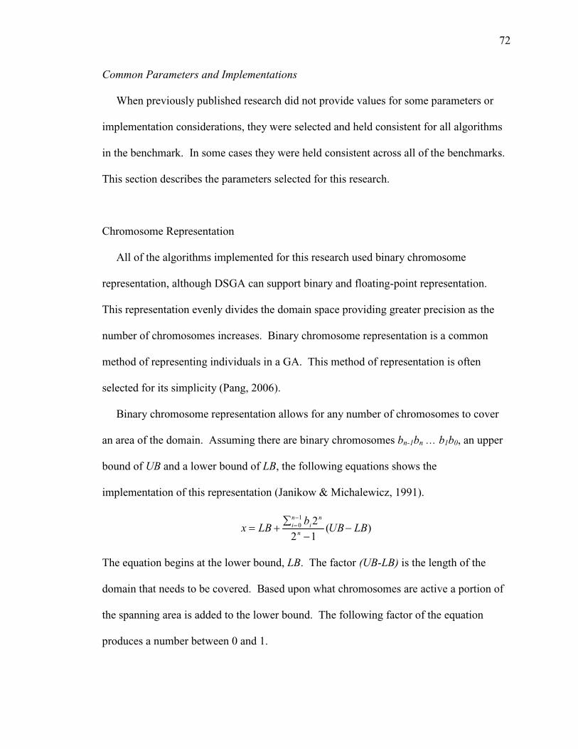
72

Common Parameters and Implementations

When previously published research did not provide values for some parameters or

implementation considerations, they were selected and held consistent for all algorithms

in the benchmark. In some cases they were held consistent across all of the benchmarks.

This section describes the parameters selected for this research.

Chromosome Representation

All of the algorithms implemented for this research used binary chromosome

representation, although DSGA can support binary and floating-point representation.

This representation evenly divides the domain space providing greater precision as the

number of chromosomes increases. Binary chromosome representation is a common

method of representing individuals in a GA. This method of representation is often

selected for its simplicity (Pang, 2006).

Binary chromosome representation allows for any number of chromosomes to cover

an area of the domain. Assuming there are binary chromosomes bn-1bn … b1b0, an upper

bound of UB and a lower bound of LB, the following equations shows the

implementation of this representation (Janikow & Michalewicz, 1991).

)(1221

0 LBUBb

LBx n

ni

ni −−

∑+=

−=

The equation begins at the lower bound, LB. The factor (UB-LB) is the length of the

domain that needs to be covered. Based upon what chromosomes are active a portion of

the spanning area is added to the lower bound. The following factor of the equation

produces a number between 0 and 1.

73

12

210

−

∑ −=

n

ni

ni b

The precision of the equation can be represented by the following equation. The ∆x term

is the smallest value that x can change.

12 −

−=∆

n

LBUBx

As the number of bits, n, increases the domain is divided into smaller sections giving

greater precision.

All of the algorithms in the research used crossover as a genetic operation. GAs can

use single-point or multiple-point crossover. All of the implemented algorithms in this

research used single-point crossover.

Fitness Function

Table 17 shows the fitness functions used in these trials for the research.

Table 17. Fitness Functions Benchmark Function Fitness Function

F1 F1 F2 F2 F3 F3 F4 F4 F5 F5 F6 F6 F7 1 / (F7 + 1) F8 F8 + 10

In the case of F1 through F6 the fitness function was the benchmark function itself.

These are all maximization problems. F7 is a minimization problem. In this case the

benchmark function of the fitness function should be inverse to each other. Benchmark

function F8 has negative values, which can cause some issues for the selection process

74

(Beasley, Bull & Martin, 1993a). The fitness function for F8 was (F8 + 10). For the

range of x equal 0 to 10, this ensures all fitness values are positive.

Other Parameters

Function F7 was previously used in Zhang et al. (2008). This research did not provide

parameters. As a result there were no control parameters for F7. The algorithms

implemented by this research used a population size of 50, created 100 generations and

had a gene mutation rate of 0.15625. Function F8 had no previously published results.

All of the algorithm results for F8 used these same parameters.

All of the results from the algorithms implemented as part of this research were the

average of 10 trials. Benchmark function F7 has a criterion of the best individual for

each niche. The results shown in the research for the algorithms are the average of the

best individual for each niche. Not all of the algorithms implemented were able to locate

all of the optima in all trials. Although it is not specifically stated in Zhang et al. (2008),

it is assumed that this algorithm located all of the optima.

Algorithm Specific Parameters and Implementations

Some parameters are specific to certain NGAs. In some cases they may span multiple

NGAs used in this research, but not all of them. When this occurred values were

selected, often from previous research, and held consistent across the benchmark. This

section addresses algorithm specific parameters.

75

Genetic Algorithm and Particle Swarm Optimization Parameters

Genetic Algorithm and Particle Swarm Optimization has three additional parameters

(Kao & Zahra, 2008). When updating a weak member with the stronger member, two

constants, C1 and C2, are needed. These constants are weights to the factors when

computing the new velocity. Kao and Zahra (2008) had them set to 2. This research kept

the values at 2. The other parameter in this algorithm was the weight for the weak

individual. This determines how much of the weak individual was maintained after the

Particle Swarm Optimization step. Kao and Zahra (2008) calculated this as 0.5 + Z / 2

where Z is a uniform random number between 0 and 1. This research kept this

calculation as well. These are the additional parameters for the Genetic Algorithm and

Particle Swarm Optimization algorithm.

Fitness Sharing Parameters

Four algorithms used a fitness sharing method: Goldberg and Richardson’s Fitness

Sharing, DSGA (R+, FS), DSGA (R-, FS) and DSGA (R∆, FS). These algorithms all

implement Goldberg and Richardson’s (1987) algorithm. The implementation of these

algorithms used the power law function, described in Chapter 2, as the fitness sharing

function. The parameters σshare and α were set to 0.1 and 1 respectively, which were the

same parameter values as in Goldberg and Richardson’s (1987).

Species Conserving Parameters

The SCGA algorithm had additional parameters. Since DSGA was based on SCGA,

these parameters are also needed in DSGA. The parameter σS defines the diameter of the

76

neighborhood. In these trials σS was set to 0.2, which makes a radius of 0.1. In DSGA

this parameter was IS. This radius was used for all benchmark functions, even F7 and F8

which have large domain areas.

DSGA Specific Parameters

DSGA has additional parameters to the SCGA algorithm. In DSGA the radius changes

as the algorithm runs. The Sigma Delta, SD, determines the change in the radius. The

SD parameter was set to 0.015 in all trials. DSGA also has a parameter, RLC. RLC or

Reevaluation Loop Count determines how many inner loops of the algorithm should be

performed before the radius is reevaluated. In trials for F1 through F6 RLC was set to 50.

This divides the total number of generations, 200, into four groups. In trials for F7 and

F8 RLC was set to 25. This divided the total number of generations, 100, into four

groups. After every RLC number of generations DSGA analyzes the last generation

seeking optima. If there CL number of identical individuals, the individual is placed on

the tabu list and considered an optima. CL was set to two in all trials. DSGA specific

parameters used in the following trials are described above.

One of the methods to vary the radius of the DSGA framework is to increase or

decrease the radius based upon information after each iteration of the inner loop

completes. While there are many different ways that this can be implemented, one

consistent method was used in this research. After each iteration of the inner loop

completes the algorithm checks to see how many individuals were added to the tabu list

through convergence. If two or more individuals were added to the tabu list, the radius

was increased by SD. Otherwise, it was decreased by SD. This implementation was

77

selected to increase the chance of finding optima. If fewer than two areas of the domain

converged, decreasing the radius would allow more seeds to be identified in future

generations and should preserve more areas of the domain.

In most GAs the final generation contains the optima that the GA has located. That is

not the case with DSGA. DSGA removes optima from the population through the use of

the tabu list. Therefore the final generation will not contain the optima located. The tabu

list contains the optima. The data provided for all benchmarks for the criterion of

proportion of peeks located for DSGA came from analyzing the tabu list, not the last

generation. The data provided for the F7 criteria of best individual in each niche also

came from the DSGA tabu list. The data for all other criteria for DSGA came from the

population.

This section describes all of the parameters used in this research. Controlled

parameters are the parameter values used in prior research. When prior research provided

parameter values, they were maintained throughout all trials. Some algorithms required

additional parameter values. These values have been described. When a parameter

existed in multiple algorithm, the parameter value was kept consistent across all trials for

a given benchmark function.

Results of Algorithms on F1

Benchmark function F1 is a sine wave with five evenly distributed local maximums all

of equal magnitude. The results for the Biggest Difference Method and Biggest

Proportion Method come from Bernier (1996) research. Table 18 shows the results for

F1. Figure 4 is a chart of the precision and recall of the algorithms.

78

Table 18. Results for Equation F1 Algorithm Recall Precision Average

fitness Bernier Biggest Difference Method 0.9800 0.7044 0.863015 Bernier Biggest Proportion Method 1.0000 0.6012 0.829098 Goldberg and Richardson’s Fitness Sharing

0.9000 0.6570 0.8590

Kao and Zahara Genetic Algorithm and Particle Swarm

0.2000 0.9890 0.9855

SCGA 0.9800 0.9250 0.9630 DSGA (R+, S-) 0.9800 0.9376 0.9714 DSGA (R-, S-) 0.9800 0.9158 0.9754 DSGA (R∆, S-) 0.9400 0.9537 0.9859 DSGA (R+, FS) 0.9800 0.9568 0.4839 DSGA (R-, FS) 0.9800 0.8749 0.9667 DSGA (R∆, FS) 0.9800 0.9425 0.9754

0

0.2

0.4

0.6

0.8

1

1.2

BDM BPM FS GAPSO SCGA DSGA(R+, S-)

DSGA(R-, S-)

DSGA(R∆, S-)

DSGA(R+, FS)

DSGA(R-, FS)

DSGA(R∆, FS)

Recall

Precision

Figure 4. Chart of Recall and Precision for F1 Bernier’s (1996) algorithms did not outperform all of the other algorithms in all

criteria. No algorithm tested could locate as many peeks as Biggest Proportion Method,

100%. However, SCGA and five of the six DSGA algorithms located 0.9800 of them,

which is the number that Biggest Difference Method found. The algorithm that had the

fewest individuals outside of the peeks was the Genetic Algorithm and Particle Swarm

Optimization algorithm. The algorithm with the highest average fitness was DSGA (R∆,

S-). However, DSGA (R+, FS) had the lowest average fitness.

79


The F2 function also is a sine wave that has five local maximums all of equal

magnitude. However, in F2 the optima are increasingly closer together. Table 19 shows

the results of the average of 10 trials for function F2. Data provided for Biggest

Difference Method and Biggest Proportion Method comes from Bernier (1996). Figure 5

shows a chart of the precision and recall.



0.9400 0.7400 0.8808


0.2200 0.9850 0.9831


As in F1 no algorithm could meet Biggest Proportion Method in locating 100% of the

peeks. The closest algorithm for this criterion was the Fitness Sharing method with

0.9400 peeks located. The Genetic Algorithm and Particle Swarm algorithm had the

fewest proportion of individuals outside of the peeks, but only found 22% of the optima.

In the average fitness criterion all of the DSGA algorithms did well with the exception of

DSGA (R+, FS).

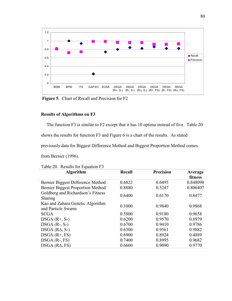
80

0

0.2

0.4

0.6

0.8

1

1.2


DSGA(R-, S-)

DSGA(R∆, S-)

DSGA(R+, FS)

DSGA(R-, FS)

DSGA(R∆, FS)

Recall

Precision

Figure 5. Chart of Recall and Precision for F2


The function F3 is similar to F2 except that it has 10 optima instead of five. Table 20

shows the results for function F3 and Figure 6 is a chart of the results. As stated

previously data for Biggest Difference Method and Biggest Proportion Method comes

from Bernier (1996).



0.6400 0.6170 0.8477


0.1000 0.9840 0.9868


81

0

0.2

0.4

0.6

0.8

1

1.2

BDM BPM FS FAPSO SCGA DSGA(R+, S-)

DSGA(R-, S-)

DSGA(R∆, S-)

DSGA(R+, FS)

DSGA(R-, FS)

DSGA(R∆, FS)

Recall

Precision


Biggest Proportion Method located all of the peeks in the function with DSGA (R-,

FS) locating the second most peeks at 0.7400. As in the previous benchmarks the

Genetic Algorithm and Particle Swarm Optimization algorithm had the least number of

individuals outside of a peek. DSGA (R∆, S-) had the greatest average fitness of the last

50 generations with a fitness of 0.9882.


The function F4 is similar to F3 except that the 10 optima are even closer together.

Table 21 shows the results of the average of the 10 trials. Figure 7 is a chart of the

precision and recall for the algorithms for F4.

For this function Biggest Proportion Method outperforms all of the other algorithms in

proportion of peeks found by at least 0.3. As in all other functions the Genetic Algorithm

and Particle Swarm Optimization algorithm produced the best results for the proportion

of points outside of the peeks. The algorithm that had the greatest average fitness in the

82

last 50 generations was the DSGA (R+, S-) algorithm. The ranking of algorithms for the

different criteria in F4 is very similar to that of F3.



0.5800 0.7170 0.8546


0.1000 0.9800 0.9852


0

0.2

0.4

0.6

0.8

1

1.2


DSGA(R-, S-)

DSGA(R∆, S-)

DSGA(R+, FS)

DSGA(R-, FS)

DSGA(R∆, FS)

Recall

Precision



Function F5 is the first function that has optima of different magnitudes. It has five

optima of decreasing fitness. Table 22 shows the results for function F5 for 10 trials of

the algorithms implemented. Figure 8 is a chart of the recall and precision.

83



0.9400 0.7580 0.5648


0.2000 0.9790 0.8165


0

0.2

0.4

0.6

0.8

1

1.2

BDM

BPM FS

GAP

SO

SCGA

DSGA

(R+, S

-)

DSGA

(R-, S-

)

DSGA

(R+, FS)

DSGA

(R-, FS

)

Recall

Precision


Three algorithms did very well in locating peeks: Biggest Difference Method, Biggest

Proportion Method and Fitness Sharing. Each located 0.9336 or more optima. All of the

other algorithms did poorly finding no more than 0.2 optima. SCGA had the most

number of individuals tracking a peek with 0.99. The algorithm with the best average

fitness was DSGA (R∆, S-).

84


Function F6 has 10 optima of decreasing fitness. The results for function F6 are

shown in Table 23. The recall and precision are shown in Figure 9.



0.8800 0.7110 0.6799


0.1000 0.9810 0.9345


Once again Biggest Difference Method, Biggest Proportion Method and Fitness

Sharing did very well at locating peeks and the other algorithms did not. SCGA did the

best at having the least number of individuals outside of the peeks and also had the

highest average fitness. The DSGA algorithms did poorly at locating peeks, finding no

more than 0.3400 of them. However, they did very well at having very high average

fitness of the last 50 generations.

85

0

0.2

0.4

0.6

0.8

1

1.2

BDM BPM FS GASPO SCGA DSGA(R+, S-)

DSGA(R-, S-)

DSGA(R∆, S-)

DSGA(R+, FS)

DSGA(R-, FS)

DSGA(R∆, FS)

Recall

Precision



The benchmark function F7 has three local optima. The global optimum is at (0, 0).

One criterion for this function is the F(x, y) value of the best individual for each of the

three optima. Since this is a minimization problem, smaller values are advantageous.

The data for the hK1 Triangulation Algorithm came from Zhang, et al. (2008). The data

for the other algorithms came from the implementation of the algorithms for this

research. The results of this test can be seen in Table 24. Figure 10 shows the recall.

Recall

0

0.2

0.4

0.6

0.8

1

1.2

hK1

Tria

ngul

atio

n

FS

SC

GA

Kao

and

Zah

ara

DS

GA

(R

+,

S-)

DS

GA

(R

-,S

-)

DS

GA

(R∆

,S

-)

DS

GA

(R

+,

FS

)

DS

GA

(R

-,F

S)

DS

GA

(R∆

,FS

)

Recall

Figure 10. Chart of Recall for F7

86

Table 24. Results for Equation F7

Algorithm F(x, y) of best individual for each

niche

Recall

Zhang, Shang, Gao and Dong hK1 Triangulation Algorithm

0.000015 0.003706 0.003706

1.0000

Goldberg and Richardson’s Fitness Sharing

0.527280 0.077355 0.94090

0.7333

SCGA 0.415233 0.000919 0.439676

0.7667


1.082841 0.000003 1.001006

0.5333

DSGA (R+, S-) 0.318560 0.000545 0.320355

1.0000

DSGA (R-, S-) 0.326982 0.003262 0.313548

0.5333

DSGA (R∆, S-) 0.372950 0.001551 0.355833

0.7000

DSGA (R+, FS) 0.324833 0.004004 0.324392

0.9667

DSGA (R-, FS) 0.325207 0.002342 0.317107

0.6000

DSGA (R∆, FS) 0.306499 0.002572 0.319992

0.6667

87

The algorithms that were implemented did not find all of the optima in all of the trials.

This was the reason that the proportion of peeks criterion is included in this results

section. Zhang, et al. (2008) did not specifically state how many optima their algorithm

located. It is assumed that all trials located all three optima.

After averaging the sum of 10 trials for each algorithm implemented, the hK1

Triangulation Algorithm did the best for optima 1 and 3. Optimum 2 was the global

minimum of (0, 0). For this optimum the Genetic Algorithm and Particle Swarm

Optimization algorithm performed best. Of the algorithms implemented only DSGA

(R+, S-) found all of the peeks in all 10 trials. This is impressive since it is only an

assumption that the hK1 Triangulation Algorithm located all of them.


Function F8 has been discussed in Chapter 1 and is the best example of the types of

functions that DSGA was developed to solve. This function has arbitrarily close optima.

Between the x values of 0 and 10, there are 16 optima. Most of the optima are within the

radius value of other optima. All of the algorithms for this benchmark function were

implemented as part of this research. The results of the average of 10 trials can be seen

in Table 25.

DSGA overwhelmingly outperformed the other algorithms in many of the criteria. All

six of the DSGA algorithms found more peeks than any of the other algorithms. The

Genetic Algorithm and Particle Swarm Optimization algorithm had the least number of

individuals outside of a peek and had the highest average fitness for the last 50

88

generations. However, for proportion of points outside of peeks and average fitness, all

DSGA algorithms did better than the Fitness Sharing algorithm.


fitness Goldberg and Richardson’s Fitness Sharing

0.4375 0.2800 1.6982


0.0875 0.8040 7.7072


0

0.2

0.4

0.6

0.8

1

1.2

FS

GAP

SO

SCGA

DSGA

(R+, S

-)

DSGA

(R-, S-

)

DSGA

(R+, FS)

DSGA

(R-, FS

)

Recall

Precision


Summary of Results

This chapter provides the results of six algorithms derived from the DSGA framework

compared to six other NGAs. Research results came from eight benchmark functional

optimization problems, seven of which had been used in prior research. The benchmark

functions covered many different functional optimization problems, including

89

minimization and maximization problems and two and three dimensional problems. Each

optimization problem used two or three criteria.

Results from the Genetic Algorithm and Particle Swarm Optimization algorithm did

poorly for most criteria. These results do not correspond to other results for this

algorithm (Kao & Zahra, 2008). Two factors could explain this. First the controlled

parameters used in Bernier (1996) may not be the best parameter settings for this

algorithm. Perhaps with a different mutation rate or population size this algorithm would

have located more optima. Kao and Zahra (2008) noted that higher mutations rates

increase the algorithm’s ability to locate optima. Second, results published in Kao and

Zahra (2008) represented individuals as a vector of real numbers instead of a binary

implementation. This research kept the chromosome representation as binary since the

other algorithms were coded using binary representations. Other research indicates that

chromosome representation can affect results in GAs (Golub, 1996). This could explain

the poor performance of the Genetic Algorithm and Particle Swarm Optimization

algorithm.

Each algorithm performed differently against this set of benchmark functions. Some

performed consistently well, others performed poorly. Appendix A Table 26 shows how

the algorithms ranked for each benchmark and criteria. A ranking of one is the best

performing algorithm. Higher ranking algorithms did not perform as well as lower

ranking ones for the given criteria. Results shown in this table for function F7 with

criteria of F(x, y) of best individuals for each niche, shows the results of the sum of the

three best F(x, y) values. While algorithm performance varied widely, no single

algorithm proved superior.

90

Chapter 5

Conclusions, Implications, Recommendations and Summary

This chapter discusses the conclusions, implications, recommendations and summary

of this research. There is a section in this chapter for each of these four topics. The

conclusion section analyzes the results against the hypothesis. The implications section

discusses the impact of this research and the contribution to the field. The

recommendations section presents future research ideas. The summary section

summarizes this research.

Conclusions

The DSGA framework was developed to solve functional optimization problems for

continuous functions when the optima are arbitrarily close. The framework allows for the

creation of multiple algorithms. There are two categories of strategies. The first category

is how to change the radius as the algorithm runs. The second category addresses how to

encourage exploration in the domain. The DSGA framework provides a foundation for

the building of a variety of algorithms to solve for arbitrarily close optima.

The first goal of this research was to develop an algorithm to solve for arbitrarily close

optima. The benchmark function F8 which is shown in Figure 1 is an example of one

such function. In this example a majority of the optima are within the radius value of

each other. All six DSGA algorithms did well in locating optima for F8. They located

91

93.13% to 95% of the optima. The three other algorithms tested only located 86.25%,

43.75% and 8.75% of the optima. The DSGA framework is remarkably good at locating

arbitrarily close optima. Results for F8 indicate that this goal was met by the DSGA

framework.

The second goal of this research was to develop an algorithm that will work equally

well for other types of problems. Excluding F8, there were 20 combinations of

benchmark functions and criteria. Six benchmark functions had three criteria and one

benchmark function had two criteria. Of these 20 combinations there were six

combinations in which a DSGA algorithm was ranked one. So, in 30% of the cases a

DSGA algorithm outperformed all other algorithms. Of the 14 combinations in which

DSGA was not ranked one, it was ranked two in seven combinations. While DSGA

algorithms did not always rank number one, results seem to indicate that it does equally

well against other types of problems.

The first hypothesis of this research was that finding optima in phases is a better

strategy for locating arbitrarily close optima. All results showed that this is a good

strategy for these types of problems. Consider the DSGA (R+, S-) and the DSGA (R+,

FS) algorithms. The beginning radius value was 0.1 and it increased by 0.015 each of the

four phases that the algorithm performed. This means that the four values of the radius

were 0.1, 0.115, 0.130 and 0.145. Of the 16 optima for F8 all but two had other optima

within these four radii. Multiple optima within a radius will cause problems for NGAs

(Ando & Kobayashi, 2005). But the two DSGA algorithms located 96.25% and 95.0% of

the optima. This occurred because each phase located some optima and removed them

from the search through the two exploration strategies to allow the algorithm to locate the

92

other optima with the remaining phases. The SCGA algorithm, which performed only

one phase, only located 86.25% of the optima. The approach to solving arbitrarily close

optima problems in phases is supported by these results.

The second hypothesis was that traditional NGAs do poorly against arbitrarily close

optima because of their use of a static radius. Changing the radius as the algorithm runs

compensates for the difficulty in solving these types of problems. Results from this

research confirmed this hypothesis. DSGA and SCGA are very similar. SCGA has a

static radius and DSGA has a dynamic radius. With the exception of benchmark function

F1, a DSGA algorithm found as many or more optima as SCGA. In F1 the distance

between optima was greater than the radius. As more optima exist within the radius, the

ability for SCGA to locate optima decreased to about half of what DSGA located.

Varying the radius as the algorithm runs helped in adjusting for poorly chosen radius

values.

Determining which DSGA strategies were the best is difficult. All six of the DSGA

algorithms performed against the benchmarks equally well. One exception to this

observation is the DSGA (R+, FS) algorithm. This algorithm consistently had an average

fitness about half of what the other DSGA algorithms had. The average fitness criterion

was the average fitness of the last 50 generations. This is a difficult criterion for DSGA,

because DSGA removes optima from the population when they are placed on the tabu

list. The DSGA (R+, FS) algorithm did perform well at locating the optima. One

explanation for this low average fitness could be in the order that DSGA (R+, FS) located

the optima. It could have located the fittest optima first and be left with the least fit ones

93

in the final generations. With a few exceptions all six DSGA algorithms performed

equally well across the benchmark criteria.

This research has demonstrated that the DSGA framework is very effective at solving

problems with arbitrarily close optima. Its ability to solve other types of problems is

comparable to other NGAs. Many factors attribute to DSGA's ability to solve such

problems. Finding optima in phases and then removing them from the search space

allows the algorithm to decompose the problem and find answers iteratively. The use of

a tabu list to store areas of the domain that have been investigated and found to be

optimal allows DSGA to encourage exploration into other areas of the domain. Changing

the radius as the algorithm executes compensates for poor radius choices that limit other

NGAs. DSGA even proved successful when all of the radius values had multiple optima

within them. Results for DSGA showed that it was successful at solving many types of

functional optimization problems.

Implications

The results of this research can be useful in a variety of areas. The DSGA framework

has been shown to be successful in locating optima for problems with arbitrarily close

optima. When it is known or suspected that a function has arbitrarily close optima a

DSGA algorithm would be appropriate in locating maximums and minimums. Results of

this research show that it locates more optima than other NGAs for these types of

problems.

Another area that the DSGA framework has implications in is when there is little or no

knowledge of where the optima are located. Without proper parameter settings many

94

NGAs have difficulty locating optima. DSGA algorithms do very well locating optima

even when the radius parameter is set incorrectly. Other NGAs have difficulties locating

optima when a poor radius parameter is selected.

This research also introduced a new benchmark function, F8. Results against other

NGAs showed that this function is difficult to solve for many NGAs. This function could

be used in future research to test other NGAs.

Recommendations

While the results of this research support the hypotheses, there are still unanswered

questions about this approach. More research could be done to provide a better

understanding of the value that DSGA has. The following are some areas where more

research is recommended.

DSGA has been tested against eight benchmark functions. While seven of the eight

functions have been used in other NGA research, DSGA has not been applied to real-

world problems. Future research could be done to test DSGA against real-world

problems like those outlined in Chapter 1: handwriting matching, electromagnetic system

design and data mining classification.

DSGA has a variety of parameters and implication considerations. In addition to

traditional GA parameters like population size, number of chromosomes and number of

generations, there are specific parameters like radius and radius delta. The fitness sharing

strategy in this researched used the power law function, but many other functions could

be used to implement this strategy. More research with other parameters and

implementation considerations could be conducted.

95

The DSGA framework enhances the SCGA algorithm. It enhances it based upon a

few principles: locating optima in phases and then excluding optima in future

generations, use of a tabu list to store optimal candidates and changing the radius as the

algorithm runs. All of these have shown to be very useful enhancements to the SCGA

algorithm, but they could be applied to other NGAs. Research that applies these

principles to another NGA would provide additional evidence that this approach is

correct.

These recommendations highlight some additional areas of research that could be

undertaken. The DSGA framework has generated six algorithms that prove to be very

useful for some types of problems. However, they have only been tested against eight

functional optimization problems. Additional research can better define the usefulness of

DSGA.

Summary

GAs can be useful tools for searching large, complex domain spaces. GAs do very

well when searching for a single optimum. But when they attempt to locate multiple

optima, they often fail. GAs have two competing forces that act upon the population.

Mutation expands the area of the domain that is being searched. This exploration

increases the area of the search space. Selection and crossover eliminate areas of the

domain and focus the search on ever shrinking areas of the domain. This exploitation

reduces the area of the search space. In every GA selection and crossover eventually win

out and the population converges.

96

Classify NGAs

NGAs are a specific type of GA that employ novel methods to prevent the exploitation

force from removing optima in the domain space. Currently there are many NGAs,

which can be classified as fitness sharing methods, crowding methods and other methods.

This research provides multiple examples of all three categories.

In fitness sharing methods special fitness functions are used. These functions alter the

fitness of individuals based upon how far they are from other individuals in the

population. More isolated individuals are given preference to increase their chances of

being selected for crossover. This provides preservation for individuals that are in low

populated areas of the domain.

A second category of NGAs is crowding methods. In crowding methods individuals

from one generation are promoted into the next generation. These individuals are often

the fittest individuals in a specific area of the domain. Crowding methods prevent the

exploitation forces of fit optimum from eclipsing weaker optima by directly maintaining

interesting individuals.

There are some NGAs that do not easily fit into the fitness sharing or crowding

categories. The other category groups these methods. Some of these methods are other

GAs that solve multiple optima problems, like Cellular Genetic Algorithms. Many

methods in this category are hybrid methods. These methods combine GAs with other

search algorithms, like the Particle Swarm Optimization and the Tabu Search. This other

category classifies NGAs that solve multiple optima problems but do not use fitness

sharing or crowding approaches.

97

DSGA Framework

One problem that many NGAs have is that when optima become arbitrarily close they

have difficulty locating all of the optima. Most NGAs have some radius parameter.

When searching the domain the parameter is used to determine how large an area of the

domain should be to make it worth preserving. The algorithm assumes that if two

individuals are within the radius, they are tracking the same optima. But this may not be

the case. An issue arises when no matter how small the radius is set to; there is some area

of the domain that has multiple optima within the radius (Ando & Kobayashi, 2005).

When this happens one optimum is often preserved and the others are lost. This makes

functional optimization problems of continuous functions that have arbitrarily close

optima difficult for NGAs to solve.

DSGA is a new NGA framework developed to solve functional optimization problems

of continuous functions that have arbitrarily close optima. The DSGA framework is

based upon the SCGA algorithm. The SCGA algorithm is a crowding NGA, but was not

developed to specifically address problems of arbitrarily close optima. The

enhancements made to SCGA are supported by other research.

SCGA is a crowding NGA. It identifies interesting individuals within a population.

These individuals are called seeds. Seeds get promoted into the next generation. Seed

selection begins by sorting a population by the fitness of each individual. Individuals are

evaluated from the fittest to the least fit. A radius parameter is used to define the area

around a seed. As individuals are evaluated, if they are not within the radius of an

existing seed, the individual is added to the list of seeds. SCGA uses normal selection,

crossover and mutation. When the next generation is created SCGA replaces members of

98

this new generation with individuals on the list of seeds. Each seed replaces the weakest

individual in the new generation that is within the radius of the seed in the domain space.

After all of the seeds are promoted into the next generation the list of seeds is empted and

individuals must compete again to be a seed. This allows SCGA to preserve these

individuals into the next generation.

DSGA enhances SCGA in a number of ways. DSGA does not attempt to locate optima

in a single loop. It runs a series of generations in an attempt to locate some optima.

Optima and seeds are placed on a short term memory structure, called a tabu list. Then it

encourages exploration into other areas of the domain to locate undiscovered optima.

DSGA has a radius parameter, which often is a limitation for most NGAs. DSGA

overcomes the problem of having multiple optima within the radius, by varying the radius

as the algorithm runs. DSGA uses two strategies to vary the radius and two methods to

encourage exploration.

DSGA has two strategies for varying the radius. It has two parameters concerning the

radius. DSGA has a radius parameter and a radius delta parameter. After a series of

generations are created, DSGA changes the radius by the radius delta parameter. The two

strategies for varying the radius are to always increase or decrease the radius and vary the

radius based upon some condition. The condition to vary the radius is arbitrary, but the

strategy was developed to use run-time information to determine if the radius should be

increased or decreased.

There are two strategies for encouraging exploration in DSGA. One is based upon the

fitness sharing method. A fitness function is defined in such a way that it decreases an

individual’s fitness the closer that the individual is to members of the tabu list. This

99

differs from other fitness sharing algorithms that vary the fitness based upon how close

individuals are to other individuals in the population. This encourages exploration into

other areas of the domain. The second strategy for encouraging exploration prevents

individuals from being seeds. If an individual is within the radius of an individual on the

tabu list, it is excluded from being a seed. These two strategies encourage exploration in

DSGA.

Research Results

The research had two goals and two hypotheses. The first goal was to develop an

NGA that could solve problems with arbitrarily close optima. The second goal was that

this NGA would perform as well as other NGAs for other types of problems. The first

hypothesis was that finding optima in phases, increases a NGAs chances of finding

arbitrarily close optima. The second hypothesis was that NGAs often miss optima in

problems with arbitrarily close optima because of static radius. Eight functional

optimization problems for continuous functions were used to test these goals and

hypotheses.

DSGA was compared to six other NGAs with eight benchmark functional

optimization problems. Each benchmark function had two or three criteria to be judged

against. One specific function had ever increasing arbitrarily close optima. In one area

of this domain the function had multiple optima within the radius.

The results of this research support the two hypotheses and show that the two goals

were met. Each of the six combinations of DSGA strategies located more optima than

any of the other algorithms tested for the benchmark function with arbitrarily close

100

optima. It even located more optima than SCGA, which shows that the ability to locate

arbitrarily close optima was not inherent in SCGA. Rather this ability came from the

enhancement that this research made in DSGA. For the other seven benchmark functions

DSGA performed equally well as other algorithms. This research indicates that locating

optima in phases works better for arbitrarily close optima and that static radius often

prevent other NGAs from locating such optima.

Conclusions

DSGA is a new NGA framework that was designed specifically to locate optima in

problems that have arbitrarily close optima. For problems in which multiple optima

existed within the radius, all DSGA algorithms located more optima than any of the other

algorithms used. DSGA does a respectable job against other functional optimization

problems. The results of this research show that the DSGA framework does very well

against functional optimization problems.

The DSGA performance comes from two factors. Locating optima in phases and then

encouraging exploration away from the located optima, simplifies the problem. This

makes locating optima easier. Varying the radius as the algorithm runs compensates for

poor radius choices. These two characteristics of DSGA make it a useful search

technique.

DSGA is a new NGA framework. It was developed to solve for functional

optimization of continuous functions when the optima are arbitrarily close. However,

DSGA results for problems that do not have arbitrarily close optima were comparable to

101

other NGAs. The DSGA framework provides a new NGA approach that leverages

existing NGA research.

102

Appendix A

Ranking of Algorithms

Table 26. Ranking of Algorithms Benchmark

Criteria Rank Ranked Algorithm

F1 Proportion of Peeks

1 Bernier Biggest Proportion Method 2 Bernier Biggest Difference Method 2 SCGA 2 DSGA (R+, S-) 2 DSGA (R-, S-) 2 DSGA (R+, FS) 2 DSGA (R-, FS) 2 DSGA (R∆, FS) 3 DSGA (R∆, S-) 4 Goldberg and Richardson’s Fitness Sharing 5 Kao and Zahara Genetic Algorithm and Particle Swarm

F1 Proportion of points outside of peaks

1 Kao and Zahara Genetic Algorithm and Particle Swarm 2 DSGA (R+, FS) 3 DSGA (R∆, S-) 4 DSGA (R∆, FS) 5 DSGA (R+, S-) 6 SCGA 7 DSGA (R-, S-) 8 DSGA (R-, FS) 9 Goldberg and Richardson’s Fitness Sharing 10 Bernier Biggest Difference Method 11 Bernier Biggest Proportion Method

F1 Average fitness

1 DSGA (R∆, S-) 2 Kao and Zahara Genetic Algorithm and Particle Swarm 3 DSGA (R-, S-) 3 DSGA (R∆, FS) 4 DSGA (R+, S-) 5 DSGA (R-, FS) 6 SCGA 7 Goldberg and Richardson’s Fitness Sharing 8 Bernier Biggest Difference Method 9 Bernier Biggest Proportion Method 10 DSGA (R+, FS)

103

Table 26. Ranking of Algorithms Continued Benchmark



1 Bernier Biggest Proportion Method 2 Goldberg and Richardson’s Fitness Sharing 3 DSGA (R+, FS) 4 DSGA (R-, S-) 5 Bernier Biggest Difference Method 6 DSGA (R∆, S-) 6 DSGA (R-, FS) 6 DSGA (R∆, FS) 7 DSGA (R+, S-) 8 SCGA 9 Kao and Zahara Genetic Algorithm and Particle Swarm


1 Kao and Zahara Genetic Algorithm and Particle Swarm 2 SCGA 3 DSGA (R+, S-) 4 DSGA (R∆, S-) 5 DSGA (R-, S-) 6 DSGA (R∆, FS) 7 DSGA (R-, FS) 8 DSGA (R+, FS) 9 Bernier Biggest Difference Method 10 Goldberg and Richardson’s Fitness Sharing 11 Bernier Biggest Proportion Method

F2 Average fitness

1 DSGA (R∆, S-) 2 DSGA (R+, S-) 3 DSGA (R-, S-) 4 DSGA (R∆, FS) 5 Kao and Zahara Genetic Algorithm and Particle Swarm 6 DSGA (R-, FS) 7 SCGA 8 Bernier Biggest Difference Method 9 Goldberg and Richardson’s Fitness Sharing 10 Bernier Biggest Proportion Method 11 DSGA (R+, FS)

104




1 Bernier Biggest Difference Method 2 DSGA (R-, FS) 3 DSGA (R+, FS) 4 Bernier Biggest Proportion Method 5 DSGA (R-, S-) 6 DSGA (R∆, FS) 7 Goldberg and Richardson’s Fitness Sharing 8 DSGA (R∆, S-) 9 DSGA (R+, S-) 10 SCGA 11 Kao and Zahara Genetic Algorithm and Particle Swarm


1 Kao and Zahara Genetic Algorithm and Particle Swarm 2 DSGA (R+, S-) 3 DSGA(R∆, S-) 4 DSGA (R-, S-) 5 SCGA 6 DSGA (R∆, FS) 7 DSGA (R-, FS) 8 DSGA (R+, FS) 9 Bernier Biggest Difference Method 10 Goldberg and Richardson’s Fitness Sharing 11 Bernier Biggest Proportion Method

F3 Average fitness

1 DSGA (R∆, S-) 2 Kao and Zahara Genetic Algorithm and Particle Swarm 3 DSGA (R-, S-) 4 DSGA (R∆, FS) 5 DSGA (R-, FS) 6 SCGA 7 DSGA (R+, S-) 8 Bernier Biggest Difference Method 9 Goldberg and Richardson’s Fitness Sharing 10 Bernier Biggest Proportion Method 11 DSGA (R+, FS)

105




1 Bernier Biggest Proportion Method 2 DSGA (R+, FS) 3 DSGA (R-, FS) 4 DSGA (R∆, FS) 5 Goldberg and Richardson’s Fitness Sharing 6 Bernier Biggest Difference Method 7 DSGA (R+, S-) 7 DSGA (R-, S-) 8 DSGA (R∆, S-) 9 SCGA 10 Kao and Zahara Genetic Algorithm and Particle Swarm


1 Kao and Zahara Genetic Algorithm and Particle Swarm 2 DSGA (R∆, S-) 3 DSGA (R+, S-) 4 SCGA 5 DSGA (R-, S-) 6 DSGA (R-, FS) 7 DSGA (R∆, FS) 8 DSGA (R+, FS) 9 Bernier Biggest Difference Method 10 Goldberg and Richardson’s Fitness Sharing 11 Bernier Biggest Proportion Method

F4 Average fitness

1 DSGA (R+, S-) 2 Kao and Zahara Genetic Algorithm and Particle Swarm 3 DSGA (R∆, S-) 4 DSGA (R-, S-) 5 DSGA (R-, FS) 6 DSGA – Dynamic Radius; Fitness Sharing 7 SCGA 8 Goldberg and Richardson’s Fitness Sharing 9 Bernier Biggest Difference Method 10 Bernier Biggest Proportion Method 11 DSGA (R+, FS)

106




1 Bernier Biggest Proportion Method 2 Goldberg and Richardson’s Fitness Sharing 3 Bernier Biggest Difference Method 4 Kao and Zahara Genetic Algorithm and Particle Swarm 4 DSGA (R+, S-) 4 DSGA (R∆, FS) 5 SCGA 5 DSGA (R-, S-) 5 DSGA (R∆, S-) 5 DSGA (R+, FS) 5 DSGA (R-, FS)


1 SCGA 2 Kao and Zahara Genetic Algorithm and Particle Swarm 3 DSGA (R-, S-) 4 DSGA (R+, S-) 5 DSGA (R∆, S-) 6 DSGA (R-, FS) 7 DSGA (R+, FS) 8 DSGA (R∆, FS) 9 Bernier Biggest Difference Method 10 Bernier Biggest Proportion Method 11 Goldberg and Richardson’s Fitness Sharing

F5 Average fitness

1 SCGA 2 DSGA (R∆, S-) 3 DSGA (R+, S-) 4 DSGA (R-, FS) 5 DSGA (R-, S-) 6 DSGA (R∆, FS) 7 Kao and Zahara Genetic Algorithm and Particle Swarm 8 Bernier Biggest Difference Method 9 Bernier Biggest Proportion Method 10 Goldberg and Richardson’s Fitness Sharing

11 DSGA (R+, FS)

107




1 Bernier Biggest Proportion Method 2 Goldberg and Richardson’s Fitness Sharing 3 Bernier Biggest Difference Method 4 DSGA (R+, FS) 5 DSGA (R∆, FS) 5 DSGA (R∆, S-) 6 DSGA (R-, S-) 7 DSGA (R-, FS) 8 DSGA (R+, S-) 9 SCGA 10 Kao and Zahara Genetic Algorithm and Particle Swarm


1 SCGA 2 Kao and Zahara Genetic Algorithm and Particle Swarm 3 DSGA (R+, S-) 4 DSGA (R∆, S-) 5 DSGA (R-, S-) 6 DSGA (R∆, FS) 7 DSGA (R-, FS) 8 DSGA (R+, FS) 9 Bernier Biggest Difference Method 10 Bernier Biggest Proportion Method 11 Goldberg and Richardson’s Fitness Sharing

F6 Average fitness

1 DSGA (R-, FS) 2 DSGA (R-, S-) 3 DSGA (R+, S-) 4 DSGA (R∆, S-) 5 DSGA (R∆, FS) 6 Kao and Zahara Genetic Algorithm and Particle Swarm 7 Bernier Biggest Difference Method 8 Goldberg and Richardson’s Fitness Sharing 9 Bernier Biggest Proportion Method 10 DSGA (R+, FS) 11 SCGA

108



F7 F(x, y) of Best Individual for Each Niche

1 Zhang, Shang, Gao and Dong hK1 Triangulation Algorithm

2 DSGA (R∆, FS) 3 DSGA (R+, S-) 4 DSGA (R-, S-) 5 DSGA (R-, FS) 6 DSGA (R+, FS) 7 DSGA (R∆, S-) 8 SCGA 9 Goldberg and Richardson’s Fitness Sharing


1 Zhang, Shang, Gao and Dong hK1 Triangulation Algorithm

1 DSGA (R+, S-) 2 DSGA (R+, FS) 3 SCGA 4 Goldberg and Richardson’s Fitness Sharing 5 DSGA (R∆, S-) 6 DSGA (R∆, FS) 7 DSGA (R-, FS) 8 Kao and Zahara Genetic Algorithm and Particle Swarm 8 DSGA (R-, S-)


1 DSGA (R-, S-) 2 DSGA (R+, S-) 3 DSGA (R∆, FS) 4 DSGA (R+, FS) 4 DSGA (R-, FS) 5 DSGA (R∆, S-) 6 SCGA 7 Goldberg and Richardson’s Fitness Sharing 8 Kao and Zahara Genetic Algorithm and Particle Swarm


1 Kao and Zahara Genetic Algorithm and Particle Swarm 2 SCGA 3 DSGA (R+, S-) 4 DSGA (R∆, S-) 5 DSGA (R-, S-) 6 DSGA (R-, FS) 7 DSGA (R+, FS) 8 DSGA (R∆, FS) 9 Goldberg and Richardson’s Fitness Sharing

109

Table 26. Ranking of Algorithms Continued

Benchmark Criteria

Rank Ranked Algorithm

F8 Average fitness

1 Kao and Zahara Genetic Algorithm and Particle Swarm 2 SCGA 3 DSGA (R∆, S-) 4 DSGA (R+, S-) 5 DSGA (R∆, S-) 6 DSGA (R-, FS) 7 DSGA (R∆, FS) 8 DSGA (R+, FS) 9 Goldberg and Richardson’s Fitness Sharing

110

Reference List

Ackley, D. H. (1987). An Empirical study of Bit Vector Function Optimization. In Davis L. (Eds.) Genetic Algorithms and Simulated Annealing (Ch. 13). Morgan Kaufman: Los Altos, CA. Alba, E., Alfonso, H. & Dorronsoro, B. (2005). Advanced Models of Cellular Genetic Algorithms Evaluated on SAT. Proceeding of the 2005 Conference on Genetic and Evolutionary Computation, Washington DC, 1123-1130. Alba, E. & Dorronsoro, B. (2008). Cellular Genetic Algorithms. Springer Science and Business Media, LLC: New York, NY. Alba, E., Dorronsoro B., Luna F., Nebro A. J. & Bouvry P. (2005). A Cellular Multi- Objective Genetic Algorithm for Optimal Broadcasting Strategy in Metropolitan MANETs. Proceedings of the 19th IEEE Internal Parallel and Distributed Processing Symposium Workshop 6, Denver CO, 192a. Ando, S. & Kobayashi, S. (2005). Fitness-based Neighbor Selection for Multimodal Function Optimization. Proceeding of the 2005 Conference on Genetic and Evolutionary Computation, Washington DC, 1573-1574. Baldwin, M. J. (1896). A New Factor in Evolution. The American Naturalist, 30(354), 441-451. Beasley, D, Bull, D. R. & Martin R. R. (1993a). An Overview of Genetic Algorithms: Part 1, Fundamentals. University Computing 15(2), 58-69. Beasley, D., Bull, D. R. & Martin, R. R. (1993b). A Sequential Niche Technique for Multimodal Function Optimization. Evolutionary Computation 1(2), 101-125. Bernier, L. (1996). A Genetic Algorithm with Self-adaptive Niche Sizing. Ottawa: National Library of Canada = Bibliothèque nationale du Canada. Bremermann, H.J. (1958). The Evolution of Intelligence. The Nervous System as a Model of its Environment (Technical Report, No.1, Contract No. 477, Issue 17). Seattle WA: Department of Mathematics, University of Washington. Burke, B. K., Gustafson, S. & Kendall, G. (2004). Diversity in Genetic Programming: An Analysis of Measures and Correlations with Fitness. IEEE Transactions on Evolutionary Computation 8(1), 47-62. Cavicchio, D. J. (1970). Adaptive Search Using Simulated Evolution. Unpublished doctoral dissertation, University of Michigan, Ann Arbor.

111

Cioffi, M., Formisano, A. & Martone, R. (2000). Distributed Niching Concept for Electromagnetic Shape Optimization by Genetic Algorithm. Proceedings of the International Conference on Parallel Computing in Electrical Engineering, Quebec. 186-190. Coello, C. A. (2000). An Updated Survey of GA-based Multiobjective Optimization Techniques. ACM Computing Surveys 32(2), 109-143. Dianati, M., Song, I. & Treiber, M. (2002). An Introduction to Genetic Algorithms and Evolution Strategies (Technical report N2L 3G1). Ontario, Canada: University of Waterloo. De Jong, K. A. (1975). An analysis of the behavior of a class of genetic adaptive systems. (Doctoral dissertation, University of Michigan). Dissertation Abstracts International, 36(10), 5140B. (University Microfilms No. 76-9381). Deb, K. & Goldberg, D. E. (1989). An Investigation of Niche and Species Formation in Genetic Function Optimization. Proceedings of the Third International Conference on Genetic Algorithms, USA, 42-50. Fonseca, C. M. & Fleming, P. J. (1993). Genetic Algorithms for Multiobjective Optimization: Formulation, Discussion and Generalization. Proceedings of the 5th

International Conference on Genetic Algorithms, 416-423. Glover, F. (1989). Tabu Search – Part I. ORSA Journal on Computing 1(3), 190-206. Glover, F. (1990a). Tabu Search – Part II. ORSA Journal on Computing 2(1), 4-32. Glover, F. (1990b). Tabu Search: A Tutorial. Interfaces 20(1), 74-94. Goldberg, D. E. & Richardson, J. (1987). Genetic Algorithms with Sharing for Multimodal Function Optimization. Proceedings of the Second International Conference on Genetic Algorithms and their Application, Cambridge Massachusetts, 41-49. Golub, M. (1996). An Implementation of Binary and Floating Point Chromosome Representation in Genetic Algorithms. Proceedings of the 18th Conference on Information Technology Interfaces, Pula, Croatia, 417-422. Hansen, M. P. (1997). Tabu Search for Multiobjective Optimization: MOTS. Proceedings of the 13th International Conference on Multiple Criteria Decision Making, Cape Town, South Africa. Holland, J. H. (1975). Adaptation in Natural and Artificial Systems. Ann Arbor, MI: University of Michigan Press.

112

Holland, J. H. (1992). Genetic Algorithms. Scientific American 267(1), 66-72. Janikow, C. Z. & Michalewicz, Z. (1991). An Experimental Comparison of Binary and Floating Point Representations in Genetic Algorithms. Proceedings of the Fourth International Conference Genetic Algorithms, 31-36. Jelasity, M. & Dombi, J. (1998). GAS, a Concept on Modeling Species in Genetic Algorithms. Artificial Intelligence, 99(1), 1-19. Kao, Y.T. & Zahara, E. (2008). A Hybrid Genetic Algorithm and Particle Swarm Optimization for Multimodel Functions. Applied Soft Computer 9, 849-857. Lee, C., Cho, D. & Jung, H. (1999). Niching Genetic Algorithm with Restricted Competition Selection for Multimodal Function Optimization. IEEE Transactions on Magnetics, 35(3), 1722-1725. Li, J. P., Balazs, M. E., Parks, G. T. & Clarkson, P. J. (2002). A Species Conserving Genetic Algorithm for Multimodal Function Optimization. Evolutionary Computation, 10(3), 207-234. Ling, Q., Wa, G., Yang, Z. & Wang, Q. (2008). Crowding Clustering Genetic Algorithm for Multimodal Function Optimization. Applied Soft Computing 8, 88-95. Mahfoud, S. W. (1995). Niching Methods for Genetic Algorithms. Dissertation. University of Illinois at Urbana-Champaign. Mauldin, M. L. (1984). Maintaining Diversity in Genetic Search. Proceedings of the National Conference on Artificial Intelligence, 247-250. McLoughlin, J. F. & Cedeno, W. (2005). The Enhanced Evolutionary Tabu Search and Its Application to the Quadratic Assignment Problem. Proceedings of the Genetic and Evolutionary Computation Conference, Washington DC, USA, 975-982. Miller, B. L. & Shaw, M. J. (1996). Genetic Algorithms with Dynamic Niche Sharing for Multimodal Function Optimization. Proceedings of IEEE International Conference on Evolutionary Computation, Nagoya, Japan, 786-791. Nebro, A. J., Durillo, J. J., Luna, F., Dorronsoro, B. & Alba, E. (2006). A Cellular Genetic Algorithm for Multiobjective Optimization. Proceeding of the Workshop on Nature Inspired Strategies for Optimization, Granda, Spain, 25-36. Nebro, A. J., Durillo, J. J., Luna, F., Dorronsoro, B. & Alba, E. (2009). MOCell: A Cellular Genetic Algorithm for Multiobjective Optimization. International Journal of Intelligent Systems 24, 726-746.

113

Oliveira, L. S., Sabourin, R., Bortolozzi, R. & Suen, C. Y. (2002). Feature Selection Using Multi-Objective Genetic Algorithms for Handwritten Digit Recognition. Proceedings of the 16th International Conference on Pattern Recognition, 367-370. Pang, T. (2006). An Introduction to Computational Physics. New York, NY: Cambridge University Press. Pozo, A. R. & Hasse, M. (2000). A Genetic Classifier Tool. Proceedings of the Twentieth International Conference of the Chilean Computer Science Society, Santiago, 14-23. Raghuwanshi, M. M. & Kakde, O. G. (2007). Distributed Quasi Steady-State Genetic Algorithm with Niches and Species. International Journal of Computational Intelligence Research, 3(2), 155-164. Rajan, C. C. & Mohan, M. R. (2002). An Evolutionary Programming-based Tabu Search Method for Solving the Unit Commitment Problem. IEEE Transactions on Power Systems, 577-585. Sheikh, R. H., Raghuwanshi, M. M. & Jaiswal, A. N. (2008). Genetic Algorithm Based Clustering: A Survey. Proceedings of the First International Conference on Emerging Trends in Engineering and Technology, Nagpur, Maharashtra, 314-319. Simoncini, D., Verel, S., Collard, P. & Clergue, M. (2006). Anisotropic Selection in Cellular Genetic Algorithms. Genetic and Evolutionary Computation Conference, Seattle WA, 559-566. Stefano, C. D., Cioppa, A. D. & Marcelli, A. (1999). Handwritten Numeral Recognition by means of Evolutionary Algorithms. Proceedings of the Fifth International Conference on Document Analysis and Recognition, Bangalore, 804-807. Ting, C. K. & Ko, C. F. (2008). Incorporating Tabu Search into the Survivor Selection of Genetic Algorithm. Proceedings of the IEEE International Conference on Systems, Man and Cybernetics 2008, Singapore, 553-558. Tsai, C. W., Tseng, S. P., Chiang, M. C. & Yang, C. S. (2009). A Time-Efficient Method for Metaheuristics: Using Tabu Search and Tabu GA as a Case. Proceedings of the Ninth Conference on Hybrid Intelligent Systems, Shenyang, China, 24-29 Whitley, D. (1993). Cellular Genetic Algorithms. Proceedings of the Fifth International Conference on Genetic Algorithms, Urbana, IL, 658. Wilcox, F. (1945). Individual Comparisons by Ranking Methods. Biometrics Bulletin 1(6), 80-83.

114

Yin, X. and Germay, N. (1993). A Fast Genetic Algorithm with Sharing Scheme using Cluster Analysis Methods in Multimodal Function optimization. In Albrecht, R. F., Steele, N. C., and Reeves, C. R., editors, Artificial Neural Nets and Genetic Algorithms, pages 450-457, Wien. Springer Verlag. Zhang, J., Shang, Y., Gao, R. & Dong, Y. (2008). An Improved Genetic Algorithm Based on hK1 Triangulation. 2008 International Seminar on Future Information Technology and Management Engineering, 73-78. Zhang, M., Zhao, S. & Wang, X. (2009). A Novel Sexual Genetic Algorithm Based on Two-Step Evolutionary Scenario of Baldwin Effect and Analysis of Global Convergence. Proceedings of the First ACM/SIGEVO Summit on Genetic and Evolutionary Computation, Shanghai, China, 737-744.

A Species-Conserving Genetic Algorithm for Multimodal Optimization

Documents

Transcript of A Species-Conserving Genetic Algorithm for Multimodal Optimization