IEEE TRANSACTIONS ON EVOLUTIONARY COMPUTATION 1

Multimodal Optimization by Means of aTopological Species Conservation Algorithm

Catalin Stoean, Member, IEEE, Mike Preuss, Member, IEEE, Ruxandra Stoean, Member, IEEE,and D. Dumitrescu

Abstract—Any evolutionary technique for multimodal opti-1

mization must answer two crucial questions in order to guarantee2

some success on a given task: How to most unboundedly3

distinguish between the different attraction basins and how to4

most accurately safeguard the consequently discovered solutions.5

This paper thus aims to present a novel technique that integrates6

the conservation of the best successive local individuals (as in the7

species conserving genetic algorithm) with a topological subpop-8

ulations separation (as in the multinational genetic algorithm)9

instead of the common but problematic radius-triggered manner.10

A special treatment for offspring integration, a more rigorous11

control on the allowed number and uniqueness of the resulting12

seeds, and a more efficient fitness evaluations budget management13

further augment a previously suggested naıve combination of14

the two algorithms. Experiments have been performed on a15

series of benchmark test functions, including a problem from16

engineering design. Comparison is primarily conducted to show17

the significant performance difference to the naıve combination;18

also the related radius-dependent conserving algorithm is sub-19

sequently addressed. Additionally, three more multimodal evolu-20

tionary methods, being either conceptually close, competitive as21

radius-based strategies, or recent state-of-the-art are also taken22

into account. We detect a clear advantage of three of the six23

algorithms that, in the case of our method, probably comes from24

the proper topological separation into subpopulations according25

to the existing attraction basins, independent of their locations26

in the function landscape. Additionally, an investigation of the27

parameter independence of the method as compared to the28

radius-compelled algorithms is systematically accomplished.29

Index Terms—Evolutionary algorithms, function optimization,30

landscape detection, multimodal optimization, species conserva-31

tion.32

I. Introduction33

MOST OF THE black-box real-world problems con-34

sidered to be difficult are multimodal. Hence, any35

optimization technique applied in this area should be able36

to discover several solutions, namely located in a number of37

basins of attraction. This enables decision makers to choose38

Manuscript received December 10, 2008; revised April 10, 2009, August12, 2009, and October 12, 2009.

C. Stoean and R. Stoean are with the Department of ComputerScience, Faculty of Mathematics and Computer Science, Universityof Craiova, Craiova 200585, Romania (e-mail: catalin.stoean@inf.ucv.ro;ruxandra.stoean@inf.ucv.ro).

M. Preuss is with the Department of Computer Science, Dortmund Uni-versity of Technology, Dortmund 44227, Germany (e-mail: mike.preuss@cs.AQ:1uni-dortmund.de).

D. Dumitrescu is with the Department of Computer Science, Babes-BolyaiUniversity, Cluj-Napoca 400084, Romania (e-mail: ddumitr@cs.ubbcluj.ro).

Digital Object Identifier 10.1109/TEVC.2010.2041668

from multiple distinct solutions to a problem and, at the 39

same time, increases confidence to have attained the global 40

optimum. Canonical evolutionary algorithms (EA)—despite 41

usually being population-based—have the property of converg- 42

ing to a population that contains only one solution and small 43

variations of it (genetic drift) [1], [2]. In the best case, the 44

fittest obtained solution represents the global optimum, but it 45

may also happen that it only refers to a local optimum in 46

which the search process is confined. In order to achieve an 47

explorative search, EAs that perform multimodal optimization 48

have to either apply multistart techniques or maintain a high 49

diversity in the population with the purpose of searching 50

within many different locations in parallel. Every multimodal 51

optimization method has to consequently satisfy two partly 52

conflicting tasks: to locate the global optimum out of multiple 53

local peaks and to find a set of several good solutions for 54

variety and insights into the problem space. 55

There have been several attempts for transforming EAs 56

so that they could deal with multimodal fitness landscapes 57

(e.g., [1], [3]–[11]). However, when tailoring such an EA, 58

there are a number of issues to be tackled: 1) how to divide 59

the population into subpopulations; 2) how to preserve 60

these subpopulations in order to avoid the genetic drift; and 61

3) how to eventually connect them to the existing optima 62

within the fitness landscape. Most techniques for the detection 63

of multiple attraction basins (niching) form subpopulations by 64

appointing a radius such that all individuals within the same 65

species lie at a distance from each other that is lower than the 66

given threshold (they are highly similar). The value that has 67

to be selected for the radius directly depends on the fitness 68

landscape, i.e., on the problem to be solved, whereas its 69

proper choice is crucial in assuring accurate results. Deb and 70

Goldberg [12] proposed a very precise approximation for this 71

parameter, however, especially for real-world applications, the 72

information on the fitness landscape required by the formula 73

is not available beforehand and, therefore, in such situations, 74

it cannot be used. Additionally, it makes the assumption of 75

equally sized, roughly spherically shaped basins of attraction. 76

In this respect, the present paper proposes a novel evolution- 77

ary method for multimodal optimization that does not employ 78

a radius for distinguishing between different species. In order 79

to detect if two individuals belong to the same subpopulation, 80

the approach makes use of their fitness evaluations and of 81

those of some intermediary assigned candidates to provide an 82

overview on their position. More importantly, this alternative 83

1089-778X/$26.00 c© 2010 IEEE

2 IEEE TRANSACTIONS ON EVOLUTIONARY COMPUTATION

triggers flexibility as regards the formation of the species84

within attraction basins of different sizes. Multiple optima85

maintenance is conducted through the preservation of several86

distinct solutions. Each species is concentrated on a seed,87

which represents the fittest individual of the species. The seeds88

from all species are copied from one generation to another so89

that no important regions are lost through selection and vari-90

ation operators. The species masters are then updated at each91

cycle, by once more appointing their fittest inner individuals.92

The manner of detecting whether two individuals follow93

different peaks or not was initially proposed in [5] and [13],94

within the multinational genetic algorithm (MGA), but the95

complete mechanism proved to be very expensive as regards96

the number of fitness evaluations necessary to converge to97

the solution [14]. On the other hand, the idea of species98

conservation first appeared in [6], however, subpopulation99

differentiation is powered by a radius.100

A first attempt to unite the seed preservation and the101

fitness landscape inspection through a straight integration was102

the topological species conservation (TSC) approach in [14].103

However, the method presented here (TSC2) is significantly104

improved as it reconsiders the species management to save pre-105

cious evaluations and accelerate convergence into the basins.106

Experimentation finally demonstrates its superiority over the107

initial naıve combination.108

The comparison is conducted on several functions that109

have at least two variables—in order to observe how the110

optimal peaks are disposed within the landscape—and up111

to 20, as most real-world problems are multidimensional.112

The multimodality conditions range from one optimum (the113

method must still not fail to perform well in the unimodal114

case) to many global or local peaks environments. Also, a115

multimodal problem that bears relationship to a generalized116

real-world application of engineering design is chosen as a117

test instance. In order to achieve an objective validation,118

the results obtained by the novel technique are put against119

those of two other related and recently proposed multimodal120

EAs [6], [7], the outcomes of a niching strategy [15], and121

those of a crowding (thus nonradius-based) approach [11].122

To demonstrate the important differences to the preliminary123

integration in [14], TSC2 is also compared to the original TSC.124

The paper is organized as follows. The next section briefly125

describes some of the traditional evolutionary approaches for126

multimodal optimization and several new ones that are relevant127

from the point of view of the design and objectives of proposed128

technique. The novel method TSC2 is presented in detail in129

Section III, also highlighting the differences to TSC. Sec-130

tion IV reports on the experimental results comparing to the131

algorithms named above, and Section V concludes the paper.132

II. Evolutionary Speciation Techniques for133

Multimodal Optimization134

In nature, an ecosystem is usually composed of regions135

(niches) that exhibit different characteristics and allow the136

formation and maintenance of different types of species.137

Commonly, the individuals in a species share similar biological138

features that allow them to coexist in their niches, capable139

of interbreeding among themselves, but unable to breed with 140

individuals from different species. Each niche is usually pop- 141

ulated by a number of individuals that directly depends on the 142

amount of resources the niche provides. 143

Analogously, in an artificial system, each niche is related to 144

an optimum of the fitness landscape and the resident species 145

contains, in the best case, only individuals being located in 146

the basin of attraction of that peak. In this respect, niching or 147

speciation methods have been proposed for the simultaneous 148

evolution of subpopulations. 149

A. Radius-Based 150

The best known niching method is the sharing approach 151

that was initially introduced by Holland [8] and subsequently 152

improved by Goldberg and Richardson [4]. The population is 153

split into several species by taking into account the similarity 154

between individuals. A sharing function modifies the fitness 155

of an individual to be dependent on the number of potential 156

solutions that exist within the same subpopulation. Within 157

the species conserving genetic algorithm (SCGA) in [6], the 158

fittest individuals that are more distant from each other than 159

a predefined radius are set as seeds of their subpopulations. 160

All other individuals (that are not seeds) are each appointed 161

to belong to the subpopulation of the fittest individual that 162

is found within the given radius. The seeds are conserved 163

from one generation to another in order to avoid the risk 164

of extinction following the application of variation operators 165

and they are updated every generation. The SCGA elitist 166

idea of transferring the seeds of each subpopulation from one 167

generation to another is also adopted in the technique proposed 168

herein. 169

Dynamic fitness sharing (DFS) is introduced in [7]. The 170

technique uses a radius for separating the population into 171

species, allows for a fixed minimum value (of two individuals) 172

for the size of a subpopulation and has, like in the case of 173

SCGA, a dominating individual called the species master. 174

This is considered to be the member of the species that has 175

the highest raw fitness value. Within DFS, the subpopulations 176

are identified in each generation using the distance between 177

individuals, while comparing it to the radius threshold. Fitness 178

sharing is employed to compute the weighted fitness of each 179

individual. A species elitist strategy is employed to ensure the 180

conservation of the most prolific individual in each subpopu- 181

lation from a generation to the other. 182

The niching variant of the covariance matrix adaptation- 183

evolution strategy (CMA-ES) of Hansen and Ostermeier [16] 184

was introduced by Shir and Back [17]. Using a fixed given 185

radius, the population is split into species by means of a 186

technique named dynamic peak identification, so that a prede- 187

fined number of q niches is generated. This largely resembles 188

a parallel execution of several independent hillclimbers at 189

different locations, separated by a distance of at least the 190

given radius. On recommendation of the authors of [10] who 191

also provided source code for the method, a niching CMA- 192

ES based on q separate (1 + 10)-CMA-ES is employed. These 193

have been proposed by Igel et al. [18], are extremely simple 194

and cope well with populations of only one parent individual. 195

The CMA-ES parameters have been shown to be very robust 196

STOEAN et al.: MULTIMODAL OPTIMIZATION BY MEANS OF A TOPOLOGICAL SPECIES CONSERVATION ALGORITHM 3

toward many forms of distortion of the optimized function,197

e.g., rotation (see the invariance discussion in [19]). However,198

no investigation of the niching parameters is found in liter-199

ature. Note that the abbreviation niching covariance matrix200

adaptation-evolution strategy (NCMA-ES) or simply NCMA201

will be used for this algorithm in the following references as202

it has not been labeled by the authors.203

B. Radius Determination204

As already mentioned earlier, Deb and Goldberg [12] sug-205

gested a way of computing the value for the σshare radius206

in charge of subpopulations differentiation, which has been207

afterwards embraced by most of the researchers dealing with208

such parameters. It uses the radius of the smallest hypersphere209

containing feasible space, which is given as210

r =1

2

√√√√ D∑i=1

(xui − xl

i)2. (1)

In (1), D represents the number of dimensions of the211

problem at hand and xui and xl

i are the upper and lower bounds212

of the ith dimension. Knowing the number of existing global213

optima NG and being aware that each niche is enclosed by a214

D-dimensional hypersphere of radius r, the niche radius σshare215

can be estimated as216

σshare =r

D√

NG

. (2)

The main drawback in using (2) for obtaining a suitable217

radius value is that it is practically impossible to know in218

advance the number of optima that exist within the fitness219

landscape. Moreover, if their attraction basins have different220

sizes and are irregularly disposed within the fitness landscape,221

then one fixed value for the radius, even if accurately de-222

termined, is not sufficient for finding and maintaining the223

different optima.224

C. Nonradius-Based225

Cavicchio’s dissertation [9] was one of the first attempts to226

use niching within genetic algorithms, by introducing a pro-227

cedure called preselection. This presumed that each obtained228

offspring had to fight for survival with the weakest parent. Five229

years later, De Jong generalized Cavicchio’s work by creating230

crowding [3]. A subset of the current population is chosen231

for every offspring, which subsequently replaces its most232

similar individual within the selected subpopulation. Variants233

like deterministic crowding [20] or probabilistic crowding234

[21] followed. The main difference between them lies in the235

way the replacement of the closest individual is performed,236

either in a deterministic or probabilistic fashion. Crowding237

was integrated within various evolutionary approaches with238

the aim of maintaining population diversity, for instance as a239

part of differential evolution in [11], where a very competitive240

approach for multimodal optimization was obtained.241

Within other approaches like the island or cellular models242

[1], the main idea is to simply separate subsets of individuals243

from the population as impelled by selection and variation244

operators. Having several subpopulations that evolve in par- 245

allel without any connectivity between them is equivalent to 246

running the same EA several times, i.e., the search process 247

could be driven to a different location in the search space each 248

time. This is the reason why, within the island model, different 249

subpopulations exchange individuals after a certain number of 250

generations. In a cellular model, the population is split into a 251

number of subregions (or neighborhoods) that are distributed 252

within algorithmic space. This is achieved by considering that 253

each individual lies on a different point on a grid and selection 254

and recombination take place only between neighbors. Note 255

that search space topology and grid topology are generally 256

entirely distinct as no measures are taken to generate a certain 257

covering of the search space. Approaches like the island or 258

cellular models keep population diversity for a longer period 259

than others, but have the main disadvantage that recombination 260

may take place between very different genotypes. It is for this 261

reason that the commonly employed evolutionary techniques, 262

like niching or crowding and other variations of them, take 263

into consideration distance within the genotypic space for 264

establishing reproduction areas. 265

An original approach that does not make use of a radius 266

and distances between genotypes when separating individuals 267

into subpopulations was developed by Ursem [5], [13]. The 268

MGA detects if two individuals track the same optimum by 269

considering a set of additional candidate solutions in-between 270

and testing if any of these is weaker than the chosen pair. 271

If this is true, a valley between the individuals is assumed 272

and consequently, they are supposed to follow different peaks 273

and will be distributed into different subpopulations. The hill- 274

valley detector unburdens the EA of using a radius and gains 275

precision and ability to overcome the irregularities in basin for- 276

mation within the fitness landscape. However, in practice, the 277

overall MGA is a high consumer of fitness evaluations [14]. 278

A final interesting alternative to radius-based paradigms 279

is brought by the cultural algorithms [22]. They determine 280

multimodality by establishing dual populations in which a 281

belief space supports contributions and in turn influences 282

future populations of individuals, which are parallelized by 283

fuzzy clustering means [23]. 284

III. Topological Species Conservation Version 2 285

Our modified algorithm, TSC2, inherits the ideas of SCGA 286

of establishing and conserving a dominating individual (seed) 287

for every species. At the same time, subpopulations differen- 288

tiation is performed through the use of the MGA component 289

to distinguish between basins of attraction. Seed dynamics are 290

furthermore controlled, both as replication and exploration are 291

concerned, but also with respect to the economy of fitness 292

evaluations that are caused by the inner workings. A naıve 293

integration was introduced in [14] as the TSC and provides the 294

starting point for improvements described herein. Although an 295

experimentally confirmed competitive multimodality detector 296

in the field, TSC lacks computational efficiency. Therefore, 297

the current TSC2 aims to become a method for species 298

differentiation based on the fitness landscape topology that 299

uses fitness evaluations much more economical. 300

4 IEEE TRANSACTIONS ON EVOLUTIONARY COMPUTATION

A. Motivation301

The efficiency of the SCGA method lies in its elitism.302

Subpopulations cannot be completely lost, even if selection303

may leave out all individuals within one species or they may304

disappear because of recombination and mutation. Conserva-305

tion of the seeds in the found species prevents them from306

going extinct. However, SCGA uses no particular mating307

selection mechanism and thus, after some generations, most308

of the individuals belong to those subpopulations that are309

connected to the fittest regions in the search space. The local310

optima are very likely to be followed exclusively by species311

containing solely the seed, which is basically conserved from312

one generation to another. Therefore, the seeds stagnate near313

local optima, without further improvement. In order to avoid314

this situation, TSC2 employs a shared fitness for mating315

selection and, as a consequence, each optimum possesses a316

subpopulation size proportional to its fitness.317

The radius-dependent trigger to differentiate subpopulations318

has been abandoned in favor of an approach that employs319

fitness discrepancies (as in MGA) mainly for two reasons.320

1) We get rid of a crucial parameter whose proper value321

is very difficult to set, especially in higher dimensional322

problems.323

2) A more flexible technique is obtained that fits the324

subpopulations better to the attraction basins of different325

sizes. Less performant individuals that are merely dif-326

ferent enough from the others are not put into distinct327

species. This is obvious especially for vast plateaus328

contained in the fitness landscape or for optima that329

have very large basins of attraction. While the SCGA330

method would form a great number of subpopulations,331

depending on the value for the radius, the MGA module332

detects only one peak to follow.333

However, the expensive behavior of the original MGA while334

detecting distinct basins of attraction is avoided. By incorpo-335

rating the preservation of diversity through seed conservation336

and efficiently keeping track of each individuals subpopulation337

during evolution, TSC2 can deal with a much smaller budget338

of fitness evaluations.339

Consequently, it borrows strength, while simultaneously340

solves inefficiencies from both these powerful methods. The341

SCGA has the weakness in the use of a radius, whereas342

the MGA has a very expensive underlying idea, if fitness343

evaluation calls are counted.344

In TSC2, distance computations between individuals now345

replace several expensive fitness calls. The number of seeds346

is restricted to a percentage of the population within TSC2, a347

restraint that did not appear either within the early integration,348

or in SCGA. This is very important for the highly multimodal349

functions, where an increased number of seeds is formed350

even from the early stages of the EA. If such a limit for351

the potential number of subpopulations were not imposed, the352

entire population could be transformed into seeds and thus353

the search blocks into local optima. Finally, TSC2 forbids354

the existence of clone seeds, and descendants are allowed to355

form their own species, adding more explorative power to the356

search, as opposed to TSC.357

B. Mechanics 358

Within the TSC2 technique, the main characteristics of a 359

species become the following. 360

1) An individual can belong to only one species. 361

2) In the ideal case, all individuals within one species lie 362

in the basin of attraction of the same optimum. This 363

certitude very much depends on the number of interme- 364

diary individuals that are considered for the verification 365

of multimodality. 366

3) Each species has a seed, which is represented by the 367

fittest individual of that subpopulation. 368

4) For each species, i.e., for all individuals it contains, a 369

unique positive integer value is assigned as ID (i.e., 370

identification). The purpose of the ID is to avoid the 371

repetition of the multimodal verification over the gener- 372

ations. 373

The method does not employ a radius for separating sub- 374

populations, however, at certain times it makes use of the 375

dissimilarity between individuals, with the purpose of reducing 376

the number of consumed fitness evaluations. In order to further 377

outline the formation of subpopulations, the mechanisms of the 378

detect-multimodal component need to be explained first. 379

1) Detect-Multimodal Method: The verification of whether 380

two points in the search space track the same optimum or 381

not is performed through an approach that was originally 382

referred to as the hill-valley mechanism [5], but which, for 383

reasons of clarity, is herein renamed to detect-multimodal. 384

The function takes two individuals (points) as arguments 385

and returns whether there is a valley between them in the 386

fitness landscape or not, i.e., they follow different peaks or 387

on the contrary. In the following, maximization is assumed, 388

but the method may be easily changed into one dealing with 389

minimization problems. 390

In order to reach a decision, a set of interior points between 391

the two given as arguments is generated. The interior points are 392

chosen based on user-defined gradations in the (0, 1) interval. 393

If the fitness values of all interior points are higher than 394

the minimal fitness of the two tested individuals, then it is 395

concluded that they track the same optimum. On the other 396

hand, if there exists such a point whose fitness is smaller 397

than the minimal fitness of the two, then it is assessed that 398

they follow different peaks. The mechanism is described in 399

Algorithm 1. f (x) denotes the fitness evaluation of individual 400

x and it is supposed that it has to be maximized. 401

In conclusion, detect-multimodal returns true if the two 402

points follow different optima and false if they track the same 403

peak. 404

The value for the number of gradations variable in Algo- 405

rithm 1 actually coincides with the number of interior points 406

that are considered. The vector gradationj contains equally 407

distant values in the (0, 1) interval. If an individual with 408

a fitness evaluation value that is smaller than the minimal 409

performance of the two initial points is found, the method 410

stops and returns true (lines 7–9). As a consequence, the 411

interior points are all evaluated only if the individuals follow 412

the same peak or when it is only the final point that has the 413

evaluation smaller than the minimal fitness of the two. 414

STOEAN et al.: MULTIMODAL OPTIMIZATION BY MEANS OF A TOPOLOGICAL SPECIES CONSERVATION ALGORITHM 5

Algorithm 1 Detect-Multimodal Mechanism Between Two Individ-uals x and y

1: i = 1;2: found = FALSE;3: while i < number of gradations and not found do4: for j = 1 to D do5: interiorj = xj + (yj − xj) · gradationj;6: end for7: if f (interior) < min{f (x), f (y)} then8: found = TRUE;9: end if

10: i = i + 1;11: end while12: return found;

Although robust, this mechanism makes an algorithm more415

expensive in terms of the number of fitness evaluations, as416

observed in MGA and TSC [14]. To counteract its effect, a free417

individual is checked against the seeds in increasing distance418

order to minimize the number of calls to the detect-multimodal419

procedure.420

An important advantage of this manner of detecting mul-421

timodality is that it avoids the existence of several subpop-422

ulations assigned to follow a certain optimum, as it happens423

when the radius-based mechanism of species conservation is424

used. Instead, it assumes the connection of a subpopulation to425

only one peak, regardless of the size of the basin of attraction426

of that optimum.427

Conversely, when TSC2 deals with a spiny function, with428

large increments followed by small decrements before rising429

again, the currently inflicted upper bound for the number of430

seeds prevents the entire population from being transformed431

(blocked) into species masters. This blockage would appear as432

a result of detect-multimodal being in charge of establishing433

them. But, with this limit, only a small part of the population434

is chosen as seeds. If other good solutions are subsequently435

found, each is assigned to the closest existing seed (according436

to the genotype) and, if fitter than the latter, it becomes the437

current species seed in the next generation.438

2) Conservation—Is It Necessary?: In every generation,439

there are a certain number of species, each having its domi-440

nating individual and following a different peak. On the one441

hand, a weighted mating selection is employed, resulting that442

the fitness of each individual is divided by the size of the443

species it belongs to. This gives a greater chance to escape444

extinction to species that have only few individuals, just like445

in Goldberg and Richardson’s fitness sharing [4].446

On the other hand, this precaution measure is not always447

sufficient, as there may exist subpopulations with few indi-448

viduals that are situated just at the base of an optimum, as449

it is the case with points x4 and x5 in Fig. 1. They may450

not be selected for recombination at all, or, if affirmative,451

might recombine with individuals from different species. In452

this way, they produce fitter offspring in other regions of the453

search space, which would eventually replace them. Therefore,454

for every subpopulation detected so far, the best individual it455

contains is retained in the next generation. However, before456

Fig. 1. Valuable individuals could vanish if not conserved.

copying such an individual, it is checked whether its instance 457

does not already exist in the population. It could have been 458

chosen through mating selection and remained unaltered in 459

the population. The insertion of these dominating individuals 460

thus happens only when they are not members of the next 461

generation, with the aim of avoiding the introduction of 462

identical prototypes in the population. 463

Concerning the preservation of the species, the new im- 464

position that the niches are kept occupied by a number of 465

individuals proportional to their resources, which is achieved 466

both within the earlier TSC and the new TSC2, by means 467

of weighted mating selection, represents a mechanism that is 468

not integrated within SCGA. Within the complementary MGA 469

[5], however, it is claimed that the selection mechanism has 470

influence upon the number of found peaks and, as a conse- 471

quence, two types of selection are chosen. One is the global 472

weighted selection and the other one is the local selection 473

within each subpopulation (nation). In the previous TSC [14], 474

both selection types are employed with the aim of keeping the 475

population properly distributed. No important influence was 476

observed as concerns the results and consequently the more 477

direct option, i.e., global weighted selection, is herein adopted. 478

As regards the annulment of multiple instances for a seed, 479

this is a very important difference of the novel TSC2 in 480

comparison to the corresponding procedure within either the 481

initial TSC or SCGA. 482

3) Determining the Species: Before referring to subpopula- 483

tions detection, the way the seeds are found must be indicated, 484

as species are formed through the gathering of individuals 485

around these dominating instances. The first generation is the 486

most expensive one as regards the used number of fitness 487

evaluations. This is the time when the detect-multimodal 488

method is applied for establishing the starting subpopulations. 489

In the next generations, until the end of the evolutionary 490

process, the species IDs are further used to reflect membership 491

wherever needed and possible. Algorithm 2 describes the 492

manner in which the seeds are selected and, at the same time, 493

the subpopulations are created around them. We denoted by n 494

6 IEEE TRANSACTIONS ON EVOLUTIONARY COMPUTATION

Algorithm 2 Seeds Selection Procedure Within TSC2Require: The current population PEnsure: The seeds

1: begin2: Sort population P decreasingly according to the fitness;3: Seeds = {P1}; (fittest individual is a seed)4: if not(first generation) then5: P1previousID

= P1ID; (previousID = the ID in the former gener-

ation)6: end if7: P1ID

= 1; (the ID of the first seed)8: currentID = 2; (currentID incremented)9: for i = 2 to n do

10: if first generation then11: Find the closest seed s in Seeds for which detect-

multimodal(Pi, s) = false;12: else13: Find the closest seed s in Seeds for which PiID = spreviousID;14: end if15: if there exists such a seed s then16: PiID = sID; (Pi belongs to the species dominated by s)17: else18: if Seeds.length < MAXSeeds then19: Seeds = Seeds ∪ {Pi}; (Pi is a seed)20: if not(first generation) then21: PipreviousID

= PiID ;22: end if23: PiID = currentID;24: currentID = currentID + 1;25: else26: Find the closest seed s in Seeds for Pi;27: PiID = sID; (integrate the individual to closest seed

species)28: end if29: end if30: end for31: return the Seeds set32: end

the population size and by Pi the ith individual in the current495

population P .496

The set Seeds is constructed by considering all individuals,497

in decreasing order of their fitness. The fittest individual498

represents the first seed that is added to the set (lines 2499

and 3). In the first generation, when an individual is taken into500

consideration in its turn, it is checked against the other existing501

seeds using the detect-multimodal mechanism, to see whether502

it follows the same peak or not. In order to save some fitness503

evaluations, TSC2 tries to avoid unnecessary applications of504

the detector and chooses the seeds by starting from the one505

closest to the current individual. The species dominated by this506

seed is, naturally, the most likely one to follow the same peak507

as the current individual. If this is not the case, the individual508

is checked against the next closest seed and so on (lines 10509

and 11).510

The seeds for all species are updated at every generation. As511

the entire population is ordered decreasingly every iteration,512

the IDs of the subpopulations do not remain identical from513

one evolutionary cycle to another. The ranking of individuals514

naturally changes, therefore, the IDs are rearranged around515

the fittest ones. The IDs start over (from 1 up to the number516

of seeds) from the fittest individual (first seed) to the least517

fit one that still represents a species master. Hence, the need 518

to retain the previous IDs for the newly set seeds (lines 4–6 519

and 20–22), so that the individuals that belong to their species 520

could be identified (line 13) and have their IDs updated (line 521

16). Thus, after the first generation, when an individual is 522

verified whether it is a seed or belongs to a certain species, it 523

is no longer the detect-multimodal procedure that checks if it 524

follows the same peak with any of the already-found seeds or 525

not. Instead, its seed ID is compared to those attributed to the 526

currently detected seeds in the previous generation specifically 527

for this purpose. When the number of seeds already reaches 528

the maximum allowed value, the newly found fit individuals 529

that follow different peaks are assigned to their closest seeds 530

in the search space (lines 26 and 27). It is by MAXSeeds that 531

the actual maximum number of seeds that may exist at a time 532

is denoted. 533

Although within TSC the species were already referred 534

through their IDs with the aim of saving an important amount 535

of fitness evaluations, TSC2 goes further in that direction by 536

comparing the individuals with the seeds that are most likely 537

to follow the same optima. 538

When the function has a large number of local optima, the 539

detect-multimodal method might generate a number of seeds 540

that is too big. That would further on block the population 541

into seeds that would only be copied from one generation to 542

another. This represents an important drawback of TSC that 543

TSC2 resolves through the limitation of the maximum number 544

of seeds to a percent of the population, fact that also counts 545

as another difference to SCGA. 546

Obviously, it cannot happen that all species are detected 547

from the first generation and kept until the end of the evolu- 548

tionary process, but new subpopulations can be discovered and 549

added to the existing ones at each iteration. The evolutionary 550

process continues with the weighted mating selection and then 551

the variation operators are applied. When mutation operates 552

on an individual, the offspring does not belong to any of 553

the existing species, i.e., it does not have a value for the 554

ID. These candidate solutions are further referred as free 555

individuals. In case of recombination, if both parents belong 556

to the same species, the offspring inherits the ID from the 557

parents. Otherwise, the descendants will be free individuals, 558

just like in the case of the offspring resulting from mutation. 559

The conservation of the species seeds follows immediately 560

afterwards and the newly created individuals with no assigned 561

ID are subsequently integrated. 562

4) Seeds Conservation: The conservation of the seeds is 563

described in Algorithm 3. Once again, f denotes the fitness 564

function to be maximized. For each seed, be that it does 565

not already have an instance in the population (line 4), it is 566

searched for the worst individual of its species, i.e., the least fit 567

individual that has the same ID value (line 5); ties are handled 568

by taking the first instance of a worst individual. If the seed has 569

a better fitness value than that individual, it enters the popula- 570

tion instead of it (lines 6–9). In case there is no such individual 571

in the population belonging to the same species, the seed is 572

introduced instead of the worst, unmarked individual in the en- 573

tire population (lines 10–13). The marking process is necessary 574

in order to avoid the deletion of already introduced seeds. 575

STOEAN et al.: MULTIMODAL OPTIMIZATION BY MEANS OF A TOPOLOGICAL SPECIES CONSERVATION ALGORITHM 7

Algorithm 3 Seeds Conservation Procedure Within TSC2

Require: The current population P

Ensure: The population that contains the seeds1: begin2: Mark all individuals in P as unprocessed;3: for every s in Seeds do4: if s does not already exist in P then5: Take worst unprocessed w from P , such that sID =

wID;6: if w exists then7: if f (w) < f (s) then8: w = s;9: end if

10: else11: Take worst unprocessed w in P ;12: w = s;13: end if14: Mark w as processed;15: end if16: end for17: return the population with the integrated seeds18: end

After detailing the TSC2 conservation mechanism, two576

differences can be identified relative to the corresponding577

procedure in the SCGA. The first modification is that no578

radius-related distance is used, since TSC2 (and the previous579

TSC, as well) verifies whether the species IDs coincide with580

those of the individuals that are to be replaced by the seeds.581

The second distinction, and also an enhancement in contrast582

to the TSC version, is made by the condition that, before583

inserting the seeds into the population, the algorithm checks584

whether a copy of their instance already exists, in order to585

prevent having duplicate individuals.586

5) Free Individuals Integration: The approach to integrat-587

ing the free individuals is described in Algorithm 4. Compared588

to the original TSC, the new procedure differs in two aspects.589

In order to avoid the inherent formation of too many species,590

which may happen only when the optimization function is591

highly multimodal, the limit for the allowed number of seeds592

is considered again. Second, it is the treatment of the free593

individuals as possible species seeds that is changed from the594

TSC way of collecting them all in a “Tower of Babel” species.595

The first choice for the integration of the individuals outside596

a species is to test whether they belong to any of the already597

existing ones. Thus, through the application of the detect-598

multimodal procedure for each free individual it is checked599

whether it follows the same peak as any of the established600

seeds. With the aim to prevent the excessive use of the detector,601

the seeds are tested in ascending distance order to the current602

individual as it more likely belongs to nearer seeds. If a seed603

that follows the same peak as the present individual is found,604

then the latter is set to belong to that seed species, takes its605

ID and is no longer free (lines 2–7).606

If individuals that do not belong to any of the existing607

species remain, then they build their own species in which they608

represent the seeds. That is done by sorting all these individu-609

Algorithm 4 Integration of the Free Individuals Within TSC2

Require: A set of free individualsEnsure: The population and Seeds set with the integrated

(formerly free) individuals1: begin2: for each free individual x do3: Find the closest seed s to x for which detect-

multimodal(x, s) = false;4: if s exists then5: xID = sID;6: end if7: end for8: if Seeds.length < MAXSeeds then9: currentID = Seeds.length + 1;

10: Find the fittest free individual x;11: Seeds = Seeds ∪ {x}; (x is a new seed)12: xID = currentID;13: while there are still free individuals and currentID <

MAXSeeds do14: For the fittest free individual x find the closest newly

added seed s for which detect-multimodal(x, s) =false;

15: if s exists then16: xID = sID;17: else18: currentID = currentID + 1;19: Seeds = Seeds ∪ {x};20: xID = currentID;21: end if22: end while23: else24: for each free individual x do25: Find the closest seed s to x;26: xID = sID; (integrate the free individual to closest

seed species)27: end for28: end if29: return the population and Seeds set with the integrated

(formerly free) individuals30: end

als in decreasing order in terms of fitness and then establishing 610

the fittest one as a new seed with the ID incremented from 611

the last species ID (lines 9–12). The next individual is then 612

verified for possible membership to the same newly created 613

species. If so, it will have the same ID assigned, otherwise, 614

it will be a new seed as well, having the next ID value. The 615

process continues for all individuals by checking them only 616

against the newly added seeds (lines 13–22). 617

If free individuals still exist, they are simply assigned to 618

the seeds closest to them (lines 23–28). This happens when 619

the maximum number of seeds has been reached. Thus, in 620

case MAXSeeds species are formed at a certain point and a 621

better solution than the existing ones is found, it enters in the 622

closest seed subpopulation that exists in the genotypic space. 623

In the next generation, this solution is chosen as the seed of 624

the species if fitter than the rest from that subpopulation. This 625

8 IEEE TRANSACTIONS ON EVOLUTIONARY COMPUTATION

Algorithm 5 Structure of TSC2

Require: A search/optimization problemEnsure: The set of seeds

1: begin2: Initialize population;3: while stop condition is not met do4: Identify species seeds; (seeds selection algorithm)5: Apply weighted mating selection;6: Apply recombination;7: Apply mutation;8: Integrate the seeds into current population; (seeds con-

servation algorithm)9: Integrate free individuals;

10: end while11: return the set of seeds12: end

way, it is conserved from one generation to another and the626

risk of extinction is eliminated.627

6) Topological Species Conservation Algorithm: After628

previously describing the main steps that are followed by629

TSC2, these are now altogether integrated in Algorithm 5. At630

each generation, before mating selection is applied, the species631

are identified and the IDs of all individuals are updated. A632

weighted mating selection is chosen in order to keep a good633

proportion between each niche resources and the individuals634

it contains. Individuals from different subpopulations are al-635

lowed to recombine, as their descendants may appear in un-636

explored regions of the search space and, in case an optimum637

lies there, they may produce new species. Conversely, when638

recombination takes place between individuals from the same639

species, as an intermediate scheme was experimentally chosen,640

the offspring is considered to belong to the same subpopulation641

as its parents, i.e., it inherits their ID. The seeds that had been642

retained in the Seeds set before the variation operators were643

applied are then integrated into the population. Finally, the644

assimilation of the descendants that do not yet belong to any645

species takes place.646

7) Extensions Beyond the Initial Integration: TSC2 differs647

from the original TSC framework [14] in the following ways.648

1) To save fitness evaluations by preventing frequent use of649

the detect-multimodal procedure, it is compared to ex-650

isting species seeds in Euclidean distance order, starting651

with the nearest.652

2) The free individuals are separately treated (and not653

during seed conservation). Their independent integration654

has the advantages that any free individual may form a655

new species and, when there exist other free individuals656

that follow the same peak, they will join the same sub-657

population. In the previous TSC version, if not members658

of an existing species, they were all included in a newly659

created, diverse subpopulation. This nonhomogeneous660

species was able to give birth to interesting solutions661

but, at the same time, many promising individuals were662

not prevented from vanishing during the evolutionary663

iterations. Within TSC2, these individuals are better664

controlled, i.e., they create their own species or, if the665

number of subpopulations reaches the upper bound, they 666

are each assigned to the species that resembles them the 667

most. 668

3) The introduction of duplicate individuals when seeds 669

conservation takes place is avoided. 670

4) An upper bound is set for the number of seeds, a fact of 671

major importance when targeting functions with spiny 672

landscapes. 673

These differences are expected to produce a major impact on 674

the obtained performance of TSC2. The initial TSC version 675

of [14] is, therefore, also considered for comparison in the 676

experiments in order to illustrate the effect of the changes. 677

8) Distinctions From Species Conservation: As compared 678

to the related SCGA, there are first the major differences and 679

improvements: speciation does not make use of a radius whose 680

value is experimentally hard to be set and the computation of 681

a high number of distances in order to identify the species 682

together with their seeds is avoided. Besides these, TSC2 does 683

not require a mechanism for achieving the final output. All the 684

seeds provided by the currently proposed approach in the end 685

of a run represent the set of solutions, in case the aim is to find 686

several global and/or local optima. This is due to the fact that, 687

within TSC2, all individuals that follow a certain optimum are 688

grouped into one species and the case that different species 689

follow the same optimum is extremely unlikely. Finally, what 690

is more, the parameter that gives the number of interior points 691

(gradations) to be considered for TSC2 is a positive integer and 692

is presumably easier to be tuned than the positive real-valued 693

radius within SCGA. However, in the experiments section, 694

direct comparison of how dependent the two connected models 695

are on these specific parameters is thoroughly conducted. 696

IV. Experimental Comparison 697

In the following set of experiments, we investigate how 698

differences in modality (one, few, and many optima), search 699

space size and the number of variables, among others, impact 700

the algorithm’s performance relative to existing ones such 701

as TSC and SCGA. In order to address relatively difficult 702

problems even with a low number of dimensions, the easiest 703

presumed case regards the optimization of functions with two 704

variables. The reason for the choices of functions in the test 705

suite was correlated with the aim to perform a deep empirical 706

study on several aspects of multimodal optimization. The goals 707

are thus to test the ability of such a technique to still be able 708

to tackle a unimodal problem, to validate its capacity to detect 709

all the global/local peaks of a function and to check the skill 710

to reach the global optimum/optima in an environment with 711

close (even spinal) local peaks. 712

All the five functions considered by the MGA [5] are 713

included in the experiments of the current paper, i.e., F1 714

(Waves), F2 (Six-Hump Camel Back), F11, F12, and F13. 715

F7 (Branin RCOS) and F8 (Shubert function) are ac- AQ:2716

quired from the SCGA experimentation [6]. The selection of 717

hard multimodal problems is extended by several functions 718

that are included in [11], namely F9 (Ackley), and F10 719

(Michalewicz). The previous F11, F12, and F13 are further 720

called by the same designations as in [11]. In addition to 721

STOEAN et al.: MULTIMODAL OPTIMIZATION BY MEANS OF A TOPOLOGICAL SPECIES CONSERVATION ALGORITHM 9

TABLE I

Considered Benchmark Functions and the Number of Dimensions D for Which They Are Tested

Common Name and Dimensions D Function Optima

Waves, 2 dimensions F1(x, y) = (0.3x)3 − (y2 − 4.5y2)xy − 4.7 cos(3x − y2(2 + x)) sin(2.5�x)) 10−0.9 ≤ x ≤ 1.2, −1.2 ≤ y ≤ 1.2

Six-Hump Camel Back, 2 dimensions F2(x, y) = −((4 − 2.1x2 + x4

3 )x2 + xy + (−4 + 4y2)y2) 6−1.9 ≤ x ≤ 1.9, −1.1 ≤ y ≤ 1.1

Sphere, 2, 10 dimensions F3(−→x ) =

D∑i=1

(−x2i ) − 5.12 ≤ xi ≤ 5.12 1

Shifted Rastrigin, 2, 10 dimensions F4(−→x ) =

D∑i=1

(x2i − 10 cos(2�xi) + 10) + f bias 1/many

−5 ≤ xi ≤ 5

Rotated Hybrid Composition F5 corresponds to function F21 in [25] 1/manyfunction, 2, 10 dimensions

Rescaled Six-hump, 2 dimensions F6(x, y) = −((4 − 2.1x2 + x4

3 )x2 + 10xy + (−4 + 4(10y)2)(10y)2) 6−1.9 ≤ x ≤ 1.9, −0.11 ≤ y ≤ 0.11

Branin RCOS, 2 dimensions F7(x, y) = (y − 5.14π2 x2 + 5

πx − 6)2 + 10(1 − 1

8π) cos(x) + 10 3

−5 ≤ x ≤ 10, 0 ≤ y ≤ 15

Shubert, 2 dimensions F8(x, y) =

5∑i=1

icos[(i + 1)x + i] ·5∑

i=1

icos[(i + 1)y + i] 18/many

−10 ≤ x, y ≤ 10

Ackley, 2 dimensions F9(x, y) = 20 + e − 20e−0.2

√x2+y2

2 − ecos(2πx)+cos(2πy)

2 1/many−30 ≤ x, y ≤ 30

Michalewicz, 2 dimensions F10(x, y) = sin(x) sin20( x2

π) + sin(y) sin20( 2y2

π) 2

0 ≤ x, y ≤ π

Ursem F1 in [5], 2 dimensions F11(x, y) = sin(2x − 0.5π) + 3 cos(y) + 0.5x 2−2.5 ≤ x ≤ 3, −2 ≤ y ≤ 2

Ursem F3 in [5], 2 dimensions F12(x, y) = sin(2.2πx + 0.5π) · 2−|y|2 · 3−|x|

2 + 5sin(0.5πy2 + 0.5π) · 2−|y|

2 · 2−|x|2 , −2.5 ≤ x ≤ 3, −2 ≤ y ≤ 2

Ursem F4 in [5], 2 dimensions F13(x, y) = 3 sin(0.5πx + 0.5π) · 2−√

x2+y2

4 , −2 ≤ x, y ≤ 2 5

Keane’s Bump Problem, 20 dimensions F14(−→x ) =

|D∑i=1

cos4(xi) − 2 ∗D∏i=1

cos2(xi)|√√√√

D∑i=1

i ∗ xi2

1/many

0 ≤ xi ≤ 10, subject to

D∏i=1

xi > 0.75 and

D∑i=1

xi <15 ∗ D

2

TABLE II

Considered Parameter Values for All Evolutionary Methods Except the NCMA-ES

Population pr /pm/ Radius/Mutation Strength No. ofSize Scaling Factor [0, 5] [0, 15] [0, 30] [0, 80] Gradations

{2, 3, . . . , 200} [0, 1] F1, F2, F6, F8, F10 F3, F4, F5, F7 F3, F4, F5, 10 dimensions F9 {1, 2, . . . , 15}F11, F12, F13 2 dimensions F14, 20 dimensions

pr and pm represent the recombination and mutation probabilities, respectively.

10 IEEE TRANSACTIONS ON EVOLUTIONARY COMPUTATION

these benchmark cases, F3 (De Jong), F4 (Shifted Rastrigin),722

F5 (Rotated Hybrid Composition function) and a shifted723

version of F2, which is presently referred to as F6, are724

further tested. In the end, a real-world problem of engineering725

design, as modeled by function F14, is included for a practical726

application of TSC2. The problems, together with the number727

of known peaks, are depicted in Table I.728

Recent model-based investigations [24] have led to the729

conjecture that complex multimodal optimization algorithms730

may perform better than simple multistart methods only if731

the number of optima is relatively low. F3 is thus tested to732

show that starting from the simplest case of only one optimum,733

the considered methods indeed perform well. Moreover, any734

method that is due to optimize a difficult function should at735

least cope with a simple one.736

Having equally distant optima would be an advantage for737

a radius-based EA, as a proper value for the radius would738

aid in detecting all peaks. But, as a real-world problem does739

not necessarily exhibit a regular fitness landscape, the original740

Six-Hump Camel Back function is rescaled in order to have741

the optima, two by two, more remote from each other (F6).742

The Waves test case is a function that is already asymmetric743

and has many peaks, some of which being even more difficult744

to find as they lie on the border or on flat hills.745

The complete description of the Shifted Rastrigin function,746

as well as the one for the Rotated Hybrid Composition747

function, can be found in [25], as they are part of a set of 25748

benchmark problems used in a contest during the Congress749

on Evolutionary Computation 2005 (Shifted Rastrigin is F9750

in the collection). The difficulty with F4 is that the global751

optimum is surrounded by a large number of very close local752

optima with only a small difference in their values as compared753

to the main peak. The F5 function represents a composition754

of five functions: Ackley, Rastrigin, Sphere, Weierstrass, and755

Griewank. According to [25], it has a huge number of optima,756

different functions properties are mixed together, the Sphere757

function adds some flat areas and a local optimum is set on758

the origin. Eleven algorithms were tested in the contest and759

none of them found the global optimum in any run when ten760

dimensions were considered. The reader is directed to [25] for761

a complete view of the function.762

Branin RCOS contains three global optima, which are763

disposed within an irregular and asymmetric landscape. Shu-764

bert’s function possesses eighteen global, equally far disposed765

optima, and many other local peaks are in between. Ackley’s766

function has one global optimum and a large number of767

local optima, as it has the appearance of a “spiny” landscape.768

Michalewicz’ function has one global optimum and a local769

one. Ursem’s F1 function contains one global optimum, a lo-770

cal peak and has a smooth landscape that should not yield dif-771

ficulties for a typical multimodal EA. Ursem’s F3 and F4 have772

each one global optimum and four local peaks. The former,773

called by Ursem “5 hills–4 valleys,” has five very close hills774

with lines of valleys between them, while the latter, named775

“1 center peak and 4 neighbors,” has the four local optima776

on the edge of the intervals and a global one in the middle.777

In order to test the applicative side of the proposed method-778

ology, Keane’s Bump problem [26] from engineering design is779

TABLE III

Considered Parameter Intervals for the NCMA-ES

Niche qeff κ (Niche Radius/MutationNumber (New Niches) Lifetime) Strength{2, . . . , 20} [1, 2] {2, . . . , 20} [0.001, 0.3 · dmax]

qeff · (q − 1)new niches are regularly introduced and live for at least kgenerations.

finally taken into consideration in the suite. The F14 function 780

has a highly bumpy surface and the global optimum is given 781

by the product constraint. 782

In summary, the test problems include: 783

1) one function with one global optimum (F3) considered 784

for 2 and 10 variables; 785

2) three functions with one global optimum and a very 786

large number of local optima, with spiny surfaces (F4, 787

F5, and F9). F4 and F5 are considered for 2 and 10 788

dimensions; 789

3) one function with 2 optima and large plateaus (F10); 790

4) five functions with several optima disposed on a smooth 791

landscape (F2, F6, F11, F12, and F13); 792

5) two functions with multiple optima that are irregularly 793

disposed, with unexpected valleys situated very close to 794

high optima (F1, F7); 795

6) one function with a large number of global optima and 796

many local ones (F8); 797

7) one function to model a real-world application and 798

chosen as a practical test (F14). 799

For F1, F2, F6, F7, F10–F13 the task is to find all optima 800

they exhibit, global, and local, while for the rest the job is to 801

concentrate the search on the global optimum/optima and to 802

escape the local, unimportant, peaks. 803

All functions are considered for maximization, there- 804

fore, when the definitions were given for minimization, the 805

functions were reversed. The constraints in Keane’s real- 806

world problem were chosen to be treated by penalizing 807

the infeasible individuals. The employed penalty function 808

reduces their fitness according to the distance to the feasible 809

region [1]. 810

A. Direct Performance Comparison 811

1) Pre-Experimental Planning: In the previous TSC ver- 812

sion [14], a maximum limit for the number of seeds was 813

not set. This parameter was revealed to be vital when it was 814

dealt with the F5 function: the results were very poor, even 815

when the test function was considered for two variables. The 816

number of seeds was exponentially increasing as generations 817

were passing. Having a population of 200 individuals, about 818

180 seeds were chosen in less than 30 generations, meaning 819

that 90% of the population was blocked from the start of 820

the algorithm. However, after setting the MAXSeeds value 821

within TSC2, this situation was successfully handled. In all the 822

undertaken experiments, an amount of 20% of the population 823

size for the value of MAXSeeds seemed to achieve a good 824

control. 825

2) Task: The first aim is to put TSC2 in contrast to the 826

original TSC version [14] and examine whether the pertained 827

STOEAN et al.: MULTIMODAL OPTIMIZATION BY MEANS OF A TOPOLOGICAL SPECIES CONSERVATION ALGORITHM 11

TABLE IV

Best/Average Results Obtained in 30 LHS Points, Each Replicated 30 Times, for Functions F1–F5

Method Peak Ratio Basin Ratio Peak Accuracy Distance AccuracyBest Avg. Best Avg. Best Avg. Best Avg.

F1, 1 global optimum, 9 local onesTSC2 0.99 0.84 1 0.88 0.13 1.84 0.04 0.79CDE 0.88 0.79 0.98 0.93 0.52 1.59 0.11 0.41TSC [14] 0.85 0.64 0.83 0.66 4.52 7.7 1.29 3.26NCMA-ES 0.8 0.49 0.9 0.59 1.85 8.89 0.88 3.87SCGA 0.66 0.18 0.99 0.264 8.74 18.59 0.98 11.56DFS 0.37 0.16 0.37 0.16 14.46 20.93 5.24 11.52

F2, 2 global, 4 local optimaTSC2 1 0.77 1 0.77 6.93e−04 2.91 0.02 2.09NCMA-ES 1 0.59 1 0.61 1.72e−03 3.9 0.02 3.19CDE 1 0.75 1 0.76 0.02 3.3 0.1 1.99SCGA 0.96 0.32 1 0.35 0.39 6.37 0.44 7.02DFS 0.67 0.26 0.67 0.26 4.64 7.27 2.73 6.22TSC [14] 0.63 0.46 0.66 0.44 3.93 6.18 3.44 6.18

F3, 2 dimensions, 1 optimumNCMA-ES 1 1 1 1 4.6e−68 3.92e−06 6.48e−35 5.84e−04CDE 1 1 1 1 9.47e−40 4.48e−04 1.96e−20 5.25e−03TSC2 1 1 1 1 5.85e−12 1.81e−07 1.61e−06 9.32e−05SCGA 1 1 1 1 1.53e−11 2.86e−07 2.41e−06 1.65e−04TSC [14] 1 1 1 1 2.48e−10 1.75e−07 4.9e−06 9.08e−05DFS 1 1 1 1 2.55e−09 4.17e−06 4.23e−05 8.12e−04

F3, 10 dimensions, 1 optimumCDE 1 0.83 1 1 2.66e−25 0.11 4.07e−13 0.15NCMA-ES 1 0.73 1 1 1.28e−17 0.08 2.51e−09 0.19TSC2 1 0.73 1 1 2.36e−06 0.15 0.001 0.23TSC [14] 1 0.74 1 1 2.79e−06 0.12 0.003 0.51SCGA 1 0.72 1 1 1.03e−05 1.43 0.003 0.45DFS 1 0.72 1 1 3.12e−05 0.14 0.005 0.22

F4, 2 dimensions, 1 global optimum/many local onesNCMA-ES 1 0.86 1 0.88 0 0.19 9.05e−9 0.14DFS 1 0.98 1 0.98 9.13e−08 0.02 7.24e−06 0.02SCGA 1 0.99 1 0.99 1.4e−07 0.01 1.46e−05 0.01CDE 1 0.88 1 0.98 4.29e−07 0.11 3.93e−05 0.03TSC2 1 0.8 1 0.94 2.23e−06 1.63 8.23e−05 0.05TSC [14] 1 0.74 1 0.93 5.04e−05 1.73 5.1e−04 0.07

F4, 10 dimensions, 1 global optimum/many local onesSCGA 1 0.35 1 0.66 0.002 18.42 0.003 1.71TSC2 1 0.04 1 0.27 0.002 39.78 0.003 2.57DFS 1 0.31 1 0.44 0.003 8.93 0.003 1.44TSC [14] 0.97 0.03 1 0.28 0.03 51.46 0.03 6.08CDE 0.9 0.12 0.97 0.19 0.09 18.68 0.04 1.68NCMA-ES 0 0 0 0 26.9 23.6 2.46 3.32

F5, 2 dimensions, 1 global optimum/many local onesTSC2 0.77 0.26 0.97 0.67 14.74 369.93 9.4e−04 0.49DFS 0.7 0.21 0.73 0.24 58.09 164.85 1.34 3.05TSC [14] 0.63 0.19 0.73 0.29 273.64 934.45 0.96 1.07SCGA 0.47 0.21 0.6 0.31 81.47 317.24 0.11 2.51CDE 0 0.003 1 0.96 20.65 134.64 0.01 0.07NCMA-ES 0 0 0 0 1700 1840 1.62 0.71

F5, 10 dimensions, 1 global optimum/many local onesNCMA-ES 0 0 0 0.01 1810 1900 9.44 8.82TSC2 0 0 0 0 770.48 1234.14 9.64 11.24DFS 0 0 0 0 569.6 870.64 11.08 12.85CDE 0 0 0 0 1076.2 1301.02 11.99 9.32SCGA 0 0 0 0.3 762.8 1311.85 12.95 11.49TSC [14] 0 0 0 0 961.59 1151.36 33.33 32.37

For each function, the methods are presented in decreasing order based on the quality of results in the best configuration, first by peak ratio and then bydistance accuracy.

12 IEEE TRANSACTIONS ON EVOLUTIONARY COMPUTATION

TABLE V

Best/Average Results Obtained in 30 LHS Points, Each Replicated 30 Times, for Functions F6–F14

Method Peak Ratio Basin Ratio Peak Accuracy Distance AccuracyBest Avg. Best Avg. Best Avg. Best Avg.

F6, 2 global, 4 local optimaTSC2 0.99 0.79 0.99 0.79 0.15 2.77 0.01 0.54CDE 0.98 0.85 0.98 0.85 0.23 1.78 0.02 0.22SCGA 0.72 0.23 0.94 0.27 3.89 7.06 0.34 5.31NCMA-ES 0.67 0.49 0.67 0.50 4.64 5.12 0.34 1.48TSC [14] 0.59 0.46 0.64 0.45 4.15 5.99 1.82 3.94DFS 0.5 0.24 0.5 0.25 4.64 6.89 0.34 4.55

F7, 3 global optimaTSC2 1 0.98 1 0.98 2.74e−07 0.02 5.54e−04 0.45DFS 1 0.72 1 0.72 6.17e−06 3.42e−04 0.003 3.63CDE 1 0.97 1 1 1.41e−05 0.1 0.004 0.21SCGA 0.99 0.62 1 0.77 0.02 0.73 0.15 6.04TSC [14] 0.96 0.75 0.94 0.85 0.8 1.79 2.43 5.48NCMA-ES 0.67 0.66 0.67 0.92 0.04 1.96 1.16 4.56

F8, 18 global, many local optimaCDE 0.99 0.27 1 0.92 0.26 115.4 0.04 3.12NCMA-ES 0.89 0.41 0.94 0.43 4.24 52.6 1.63 31.0TSC2 0.7 0.3 0.81 0.3 99.07 727.9 4.23 33.2DFS 0.44 0.21 0.44 0.21 0.04 0.11 44.55 88.2TSC [14] 0.36 0.13 0.26 0.21 750.8 1628.46 78.8 59.2SCGA 0.27 0.08 0.3 0.32 589.7 1381.05 42.75 22.1

F9, 1 global, many localNCMA-ES 1 0.97 1 1 0 0.01 2.56e−16 2.96e−03DFS 1 1 1 1 4.14e−05 0.003 1.46e−05 8.18e−04SCGA 1 1 1 1 4.61e−05 0.003 1.63e−05 9.78e−04TSC2 1 0.72 1 1 2.25e−04 0.85 7.95e−05 0.21TSC [14] 1 0.91 1 1 0.001 0.23 4.18e−04 0.06CDE 1 0.69 1 0.98 0.001 0.24 4.61e−04 0.05

F10, 1 global, 1 localTSC2 1 0.99 1 0.99 1.01e−07 0.009 7.83e−05 0.02NCMA-ES 1 0.93 1 0.93 6.87e−08 0.07 9.41e−05 0.15CDE 1 1 1 1 1.71e−07 0.006 1.18e−04 0.01TSC [14] 1 0.99 1 0.99 1.08e−06 0.01 2.4e−04 0.03DFS 1 0.6 1 0.62 8.0e−04 0.37 0.005 0.72SCGA 1 0.58 1 0.63 0.002 0.48 0.007 0.92

F11, 1 global, 1 localCDE 1 1 1 1 2.87e−07 0.002 2.83e−04 0.009TSC2 1 0.97 1 0.97 3.82e−07 0.1 6.04e−04 0.21NCMA-ES 1 0.75 1 0.75 4.23e−07 0.64 6.49e−04 1.42TSC [14] 1 1 1 1 3.87e−07 0.005 7.67e−04 0.01DFS 1 0.65 1 1.66 6.31e−07 0.92 8.12e−04 1.87SCGA 0.98 0.75 1 0.76 0.006 0.76 0.03 1.55

F12, 1 global optimum, 4 local onesCDE 1 0.97 1 0.98 0.003 0.1 0.01 0.12TSC2 1 0.94 1 0.94 0.008 0.32 0.03 0.34NCMA-ES 1 0.55 1 0.69 0.01 1.89 0.04 1.99SCGA 0.99 0.33 1 0.38 0.07 4.28 0.15 4.32TSC [14] 0.96 0.68 0.94 0.67 0.2 1.68 0.28 1.77DFS 0.81 0.28 0.79 0.3 0.17 4.3 0.2 4.29

F13, 1 global optimum, 4 local onesCDE 1 0.97 1 0.98 5.89e−04 0.12 0.001 0.36TSC2 1 0.94 1 0.93 8.33e−04 0.28 0.001 0.95NCMA-ES 1 0.56 1 0.56 1.02e−03 1.02 0.002 5.42DFS 0.99 0.38 1 0.38 0.07 2.11 0.15 7.36TSC [14] 0.99 0.84 0.89 0.64 0.15 0.89 1.22 7SCGA 0.89 0.32 1 0.49 0.37 2.53 0.54 7.68

F14, 20 dimensions, 1 global, many localTSC2 1 0.03 0.13 0.42 0.05 0.46 3.2 8.73NCMA-ES 1 1 1 1 0 0 6.6 10.4SCGA 0.97 0.25 0.17 0.48 0.04 0.29 3.22 7.49CDE 0.9 0.6 0.93 0.53 0.05 0.23 1.15 4.16DFS 0.87 0.04 0 0.09 0.07 0.35 3.98 7.63TSC [14] 0.5 0.02 0.2 0.66 0.11 0.51 10.18 34.8

For each function, the methods are presented in decreasing order based on the quality of results in the best configuration, first by peak ratio and then bydistance accuracy.

STOEAN et al.: MULTIMODAL OPTIMIZATION BY MEANS OF A TOPOLOGICAL SPECIES CONSERVATION ALGORITHM 13

TABLE VI

p-Values Calculated by Means of t-Test and Wilcoxon

Rank-Sum Test for TSC2 Versus the Others for F1–F5

TSC2 Peak Ratio Distance AccuracyVersus t-Test Wilcoxon t-Test Wilcoxon

F1, 1 global optimum, 9 local ones+CDE 2e−08 1.8e−08 – –+TSC [14] 2.7e−10 2.7e−09 – –+NCMA-ES <2.2e−16 6.1e−14 – –+SCGA <2.2e−16 1.9e−12 – –+DFS <2.2e−16 1.9e−12 – –

F2, 2 global, 4 local optima+NCMA-ES – – 0.71 0.01+CDE – – <2.2e−16 <2.2e−16+SCGA 0.02 0.01 <2.2e−16 <2.2e−16+DFS – 1.69e−14 – –+TSC [14] 3.1e−12 9.1e−13 – –

F3, 2 dimensions, 1 optimum−NCMA-ES – – 4.2e−05 <2.2e−16−CDE – – 4.2e−05 <2.2e−16+SCGA – – 4.8e−07 0.28+TSC [14] – – 0.24 2.6e−07+DFS – – 3.5e−04 1.2e−14

F3, 10 dimensions, 1 optimum−CDE – – 1.5e−12 <2.2e−16−NCMA-ES – – 1.5e−12 3.1e−11+TSC [14] – – 3.7e−04 7.7e−05+SCGA – – 2.1e−04 2.3e−04+DFS – – 5.8e−15 8.6e−15

F4, 2 dimensions, 1 global optimum/many local ones−NCMA-ES – 1.69e−14 0.34 6.4e−08-DFS – – 0.34 6.9e−11-SCGA – – 0.34 2.3e−11−CDE – – 0.34 4.1e−05+TSC [14] – – 0.34 9.8e−04

F4, 10 dimensions, 1 global optimum/many local ones-SCGA – – 0.35 0.53+DFS – – 0.008 0.02+TSC [14] 0.33 0.33 2.1e−12 <2.2e−16+CDE 0.08 0.08 0.23 3.6e−10+NCMA-ES – – <2.2e−16 3.1e−11

F5, 2 dimensions, 1 global optimum/many local ones+DFS 0.57 0.57 6.8e−04 0.62+TSC [14] 0.27 0.27 1.5e−04 0.22+SCGA 0.02 0.02 0.04 0.84+CDE 1.1e−10 1.5e−09 – –+NCMA-ES 1.1e−10 1.5e−09 – –

F5, 10 dimensions, 1 global optimum/many local ones−NCMA-ES – – 0.19 0.18+DFS – – 0.008 0.19+CDE – – 3.9e−07 2.1e−07+SCGA – – <2.2e−16 6.3e−15+TSC [14] – – <2.2e−16 <2.2e−16

When the peak ratio difference is not significant, distance accuracy is alsoconsidered. +/− stands for TSC2 being better/worse.

modifications indeed yield the expected significant difference828

in results. Secondly, it is targeted to perform a direct com-829

parison between the radius-dependent species conservation830

technique of inspiration, the SCGA, and the novel radius-free831

TSC2 approach. The MGA was not used in the comparison832

here because previous work [14] had shown that it was less833

efficient than both SCGA and the earlier TSC formulation in834

terms of acquired performance relative to the number of spent835

fitness evaluations. Additionally, two other radius-propelled836

evolutionary techniques were taken for a contrast: DFS, which837

was very competitive in the experiments described in [7] and838

TABLE VII

p-Values Calculated Through a t-Test and a Wilcoxon

Rank-Sum Test for TSC2 Versus the Others for F6–F14

TSC2 Peak Ratio Distance AccuracyVersus t-Test Wilcoxon t-Test Wilcoxon

F6, 2 global, 4 local optima+CDE 0.65 0.65 0.08 3.5e−07+SCGA 3.2e−10 3.1e−10 – –+NCMA-ES <2.2e−16 4.1e−14 – –+TSC [14] 1.9e−14 3.3e−12 – –+DFS <2.2e−16 4.1e−14 – –

F7, 3 global optima+DFS – – 6.1e−04 3.0e−05+CDE – – 7.8e−04 9.7e−14+SCGA 0.33 0.33 8.9e−08 <2.2e−16+TSC [14] 0.04 0.04 0.004 <2.2e−16+NCMA-ES – – <2.2e−16 7.6e−12

F8, 18 global, many local optima−CDE <2.2e−16 6.4e−12 – –−NCMA-ES 2.1e−13 1.5e−10 – –+DFS <2.2e−16 2.1e−11 – –+TSC [14] <2.2e−16 2.2e−11 – –+SCGA <2.2e−16 1.8e−11 – –

F9, 1 global, many local−NCMA-ES – – 0.005 3.0e−11−DFS – – 0.009 8.9e−05−SCGA – – 0.009 2.6e−04+TSC [14] – – 0.02 0.005+CDE – – 0.1 0.002

F10, 1 global, 1 local+NCMA-ES – – 0.13 0.008+CDE – – 6.7e−09 4.1e−10+TSC [14] – – 0.32 3.1e−13+DFS – – 1.2e−08 <2.2e−16+SCGA – – 4.5e−07 <2.2e−16

F11, 1 global, 1 local−CDE – – 1.8e−06 6.8e−06+NCMA-ES – – 0.53 0.02+TSC [14] – – 0.92 0.18+DFS – – 0.04 7.3e−04+SCGA – – 1.4e−09 <2.2e−16

F12, 1 global optimum, 4 local ones−CDE – – 6.4e−09 3.6e−09+NCMA-ES – – 2.4e−06 1.5e−05+SCGA 0.32 0.32 1.1e−11 <2.2e−16+TSC [14] 0.03 0.02 3.2e−04 4.9e−11+DFS 1.99e−09 1.32e−09 – –

F13, 1 global optimum, 4 local ones−CDE – – 3.1e−15 3.5e−14+NCMA-ES – – 0.03 2.6e−06+DFS – – 0.16 4.9e−11+TSC [14] 0.33 0.33 0.003 <2.2e−16+SCGA 9.1e−05 2.7e−05 – –

F14, 20 dimensions, 1 global, many local+NCMA-ES – – <2.2e−16 1.2e−12+SCGA 0.33 0.33 0.06 0.1+CDE 0.08 0.08 2.8e−10 1.6e−09+DFS 0.04 0.04 0.17 0.2+TSC [14] 8.7e−06 9.6e−06 – –

When the peak ratio difference is not significant, distance accuracy is alsoconsidered. +/− stands for TSC2 better/worse.

is fundamentally related to TSC2, and the NCMA-ES, which 839

achieved very good results within validation [15]. In order 840

to also have a completely different method to weigh against, 841

the crowding differential evolution (CDE) presented in [11] 842

is also included in the comparison. The method does not 843

possess a radius, but it has a different parameter, the scaling 844

14 IEEE TRANSACTIONS ON EVOLUTIONARY COMPUTATION

factor, that is used for creating new offspring. Consequently,845

the hypotheses to be tested are as follows.846

1) The enhanced TSC2 is more efficient than the initial847

TSC combination in [14], in terms of the balance848

between the achieved performance and the number of849

invested fitness evaluations.850

2) TSC2, having an additional parameter that must be a851

positive integer and represents a several-choice number852

of individuals, is at least as good as SCGA, DFS, and853

NCMA-ES, all three with a radius parameter that is real,854

free-valued.855

3) TSC2 has significantly better performance on several856

types of test problems than the methods of comparison.857

Accordingly, the conditions under which TSC2 is able858

to outperform the others are identified.859

3) Experimental Setup: In order to achieve an objective860

comparison, the only user interaction in setting the parameters861

for the examined techniques appears in defining the ranges862

for their values. The statistical method of Latin hypercube863

sampling (LHS) (e.g., [27]) is employed to generate a space-864

filling (fair) sample of the algorithm parameters. For small865

sample sizes, it is well known to generate more even distribu-866

tions than random sampling. For this reason, it is also the first867

step in the tuning algorithm sequential parameter optimization868

(SPO) [28]. Here, we use it to generate a disposition of869

plausible parameter sets from a multidimensional distribution,870

which is conducted on all test functions for automatically871

setting the values for every involved parameter within all872

compared methods. It is clear that there is further room for873

improvement of algorithm parameters by applying a full tuning874

method, but the LHS already gives a good estimation of the875

performance values under parameter variation. Thereby, we876

can avoid comparing algorithms under bad parameter settings.877

For all considered test functions and all techniques, we878

employ the same budget of 3×104 fitness evaluations. For all879

methods, except NCMA-ES, the evolutionary variables are set880

as follows. The upper bound of the population size is restricted881

to 200. The mutation and crossover probabilities are selected882

by the LHS in the interval [0, 1] in all experiments. The upper883

limit for the mutation strength parameter is similarly set for884

all compared techniques, but differently for each benchmark885

function. The interval from which the LHS takes the values886

for the mutation strength is actually identical to the one of the887

radius parameter within the SCGA and DFS, which depends888

on the problem to be solved. The radius value is computed889

for each function using the Deb and Goldberg formula (1)890

and then the upper bound of the interval is appointed as891

approximately the double of that value, in order to make sure892

a proper configuration is included in the ones generated by the893

LHS. For all benchmark problems, the number of gradations894

in TSC2 is considered from the set {1, 2, . . . , 15}. Table II895

illustrates the sets and intervals used for each tuned parameter.896

For the NCMA-ES, parameter intervals (Table III) have to897

be chosen in a different fashion as it knows no base population898

but only niches holding one individual each. Furthermore,899

the probabilities for mutation and crossover cannot be easily900

changed. Mutation is usually always done in CMA-ES vari-901

ants, and recombination is implicitly performed in one step 902

with selection. However, the NCMA-ES possesses other pa- 903

rameters, namely qeff and κ. The first one resembles the num- 904

ber of total niches, that is the number of “stable” niches plus a 905

number of “test” niches. In contrast to the additive fashion that 906

would lead to unwanted dependencies on the original niche 907

number, a multiplier in the interval [1, 2] is used to compute 908

qeff as the product of this parameter and the number of “stable” 909

niches. The second one, κ, is set as the discrete minimum lifes- 910

pan of the “test” niches between 2 and 20. The initial stepsize 911

and the niche radius are varied in the interval of [0.001, 0.3] · 912

dmax, the latter meaning the maximum search space expansion 913

in one dimension. These values have been chosen according 914

to the recommendation of the authors of [10]. 915

There are 30 LHS points taken into account for each test 916

function and every configuration is replicated 30 times for 917

all techniques in turn. The average over the 30 repeated runs 918

of the best configuration and the mean over all 30 different 919

configurations are recorded. The latter is reported to indicate 920

how sensitive each technique is to changes in the parameter 921

values. It does not necessarily demonstrate the superiority of 922

a method upon another, but shows that tuning the methods 923

can require different amounts of effort, where one that gives 924

good results for a large variety of configurations shall be 925

preferred. Naturally, if the number of parameters is smaller, the 926

available space is explored better when the number of tested 927

configurations is held constant. 928

A peak is considered as found if at least one individual of 929

the population of the last generation is situated in the basin 930

of attraction of that optimum, with an accuracy of at least 931

10−1. Several measures are used for evaluating success of the 932

different algorithms. 933

1) The peak ratio computes the fraction between the num- 934

ber of detected peaks and the amount of peaks to be 935

found. 936

2) Basin ratio is meant to be broader than the previous 937

measure, as it counts a basin as found if an individual 938

entered the basin, even if not closer than 10−1 in fitness. 939

When an individual is in the right basin, it will most 940

likely find the desired peak with a few more evaluations. 941

We detect an individual inside a basin via the detect- 942

multimodal method with ten interior points. The actual 943

measurement is given as ratio between the number of 944

detected basins and the number of desired optima (and 945

basins, accordingly). 946

3) The peak accuracy measure is calculated as follows. For 947

each optimum to be found, the nearest individual x in 948

the population is taken and the absolute difference in 949

fitness values is computed. Then, all these differences 950

are summed as in (3), where the fitness of an individual 951

x is denoted by f (x) 952

peak acc. =#peaks∑

i=1

| f (peaki) − f (x) |. (3)

4) When there are more peaks that have very close or 953

identical peak height, the previous metric may produce 954

good results even if all the population is situated in 955

STOEAN et al.: MULTIMODAL OPTIMIZATION BY MEANS OF A TOPOLOGICAL SPECIES CONSERVATION ALGORITHM 15

the basin of the attraction of the same peak. As a956

precaution, the distance accuracy that refers to the957

dissimilarity in the genotypic space between each peak958

and its closest individual is also computed and stands959

for a ranking field of compared methods. It is derived960

in the same manner as in (3), with the only change961

that the difference between fitness values is substituted962

by the Euclidean distance between the two individuals.963

Current and previous measure should stay poised, or964

otherwise, a peak accuracy error caused by coincidental965

close evaluations may appear.966

The first two measures were also considered in [5], the third967

appears in [11] and the last is proposed herein.968

Besides the newly proposed TSC2 approach, the other tech-969

niques considered for comparison have also been implemented970

by the current authors. The only exception is the NCMA-ES971

whose code, made available by its authors, was interfaced.972

Additionally, the same type of (common) operators [1] are973

employed for all algorithms (except NCMA-ES).974

1) Binary tournament selection.975

2) Intermediate recombination with probability pr, so that976

the genes of an offspring O are obtained from two par-977

ents P and Q according to (4), where R is a uniformly978

distributed random number over [0, 1]979

O = P + R · (Q − P). (4)

3) Mutation with normal perturbation with probability pm.980

A gene of an individual X selected to be modified981

through mutation is changed according to (5). MS and982

N(0, 1) represent the mutation strength and a normally983

distributed random variable with expected mean 0 and984

variance 1, respectively985

X′ = X + MS ∗ N(0, 1). (5)

4) Results: The results derived from the LHS986

parameterization are depicted in Tables IV and V. While for987

peak ratio and basin ratio, higher values signify better results988

(1 being the best), for the other two measures, better results989

correspond to smaller values, meaning that the individuals990

came closer to the actual solutions in accuracy (see peak991

accuracy), as well as in genotype (distance accuracy). The992

best configuration of a method refers first to the peak ratio993

results, then, in case of equality, it is chosen with respect994

to the distance accuracy. The corresponding values from the995

best basin ratio and best peak accuracy are the ones obtained996

in the configuration that is chosen to be the best with respect997

to the peak ratio or distance accuracy. Besides the average998

results of the best configuration repeated 30 times, the mean999

over all generated design points, each replicated 30 times,1000

is presented. For each function, the techniques involved1001

in the comparison are ranked upon the quality of the best1002

configuration results, these too ordered first by peak ratio and1003

then by distance accuracy. The best result with respect to1004

each of the four applied measures is highlighted.1005

Fig. 2 enables a quick visual comparison for the best1006

configuration of relative distance and peak accuracies of every1007

function over all algorithms.1008

In order to verify the significance of the results and to 1009

validate the hypotheses formulated in the task subsection, two 1010

statistical tests are conducted for the results obtained in the 1011

30 repeats of the best configurations. A t-test for independent 1012

samples is used to compare the difference in means between 1013

TSC2 and every other algorithm. As the normality assumption 1014

may not hold, the Wilcoxon rank-sum test is employed as 1015

a nonparametric alternative. The tests are performed on the 1016

peak ratio (best LHS configuration repeated 30 times). If two 1017

algorithms are not significantly different concerning this mea- 1018

sure, their distance accuracies are also tested. The statistical 1019

results for all the functions are presented in Tables VI and VII. 1020

In these two tables, the methods are ordered according to 1021

the quality of their results as reported in Tables IV and V. 1022

The labels + or − assigned to each referenced technique 1023

signify the fact that TSC2 obtained better or worse results 1024

in comparison to it. 1025

5) Observations: A brief look over Tables IV and V 1026

confirms that the compendium of benchmark functions is well 1027

chosen. Note that the method rankings change, depending on 1028

the problem properties, i.e., dimensionality, multimodality, and 1029

deceptive character. 1030

We now analyze result Tables IV and V and the significance 1031

Tables VI and VII with the purpose of identifying for what 1032

problem types TSC2 performs significantly better than the 1033

other algorithms. TSC2 is placed first, or ex aequo with 1034

results similar (according to the statistical tests) to the method 1035

ranking first, for F1, F2, F4 with 10 variables, F5 with 1036

two variables, F6, F7, F10, and F14. The only other cases 1037

that have multiple peaks, all to be found, are F11, F12, and 1038

F13 and for these TSC2 is second best, with only minor (but 1039

statistically significant) differences in distance accuracy below 1040

CDE. Most of these functions have an irregular landscape, with 1041

optima often situated on the margins of the intervals, facts that 1042

disadvantage the other, radius-based methods. F8 is a different 1043

case because, although it has 18 global optima to be detected, 1044

it also possesses many local optima that are to be omitted. 1045

Nevertheless, the result for this case places TSC2 third out of 1046

the six techniques as regards the number of discovered peaks. 1047

The proposed technique does not disappoint for the remaining 1048

functions either, as it gives competitive results in most of the 1049

cases. Nevertheless, TSC2 seems best suited for the test cases 1050

with irregular landscapes that have up to 10 optima, all of 1051

which have to be located. 1052

For the above mentioned test cases with optima haphaz- 1053

ardly disposed, like F1, F6, F7, F11, F12, and F13, TSC2 1054

is more accurate in finding the peaks than the radius-based 1055

techniques. CDE is outperformed by TSC2 when there is 1056

one optimum to be detected that has many local peaks in 1057

its vicinity and the discrepancy becomes higher when the 1058

number of dimensions raises to 10 or 20. To continue with 1059

the clarifications regarding the formulated hypotheses, TSC2 1060

is superior to TSC [14] in all considered test cases. Checking 1061

the significance of the difference in results from Tables VI 1062

and VII, the only cases where TSC2 is not statistically 1063

better are F9 and F11; however, the resulting values still 1064

place the new technique above its previous version in the 1065

standings. 1066

16 IEEE TRANSACTIONS ON EVOLUTIONARY COMPUTATION

Fig. 2. Overview of relative (a) distance and (b) peak accuracies for the best LHS configurations of each algorithm. Results are log 10-transformed and thenseparately normalized for each problem, so that 0.0 refers to the best and 1.0 to the worst algorithm. Both measures lead to similar impressions, with threepredominant algorithms: CDE, NCMA-ES, and TSC2.

Fig. 3. Log 10-transformed distance accuracies of 30 runs of TSC2 against 30 runs of TSC. Best LHS configurations are compared over all test problems.TSC2 is better except for two cases.

STOEAN et al.: MULTIMODAL OPTIMIZATION BY MEANS OF A TOPOLOGICAL SPECIES CONSERVATION ALGORITHM 17

TABLE VIII

Overall Best/Average Results Obtained for Classes of Test Functions

Method Peak Ratio Basin Ratio Peak Accuracy Distance AccuracyBest Avg. Best Avg. Best Avg. Best Avg.

One optimum, F4 2 and 10 dimensions, F5 2 and 10 dimensions, F9, F14TSC2 4.77 1.85 4.1 3.3 785.27 1646.8 12.97 23.29DFS 4.57 2.54 3.73 2.75 627.76 1044.8 16.13 24.99SCGA 4.44 2.8 3.77 3.74 844.31 1647.8 17.8 23.21TSC [14] 4.1 1.89 3.93 3.16 1235.4 2139.7 44.26 74.45CDE 3.8 2.29 4.9 3.64 1097 1454.9 13.19 15.31NCMA-ES 3 2.83 3 2.89 3516.8 3742.6 20.12 23.39

Multiple optima, F1, F2, F6, F7, F10–F13TSC2 7.98 7.22 7.99 7.25 0.29 8.25 0.12 5.39CDE 7.86 7.3 7.96 7.5 0.77 7 0.25 3.33SCGA 7.19 3.33 7.93 3.91 13.49 40.8 2.64 44.4NCMA-ES 7.14 5.02 7.24 5.55 6.55 23.49 2.44 22.08TSC [14] 6.98 5.82 6.9 5.7 13.75 24.25 10.48 27.67DFS 6.34 3.29 6.33 4.35 23.98 42.79 8.67 40.16

More than 2 dimensions, F3, F4, F5, F14TSC2 3 0.8 2.13 1.69 770.5 1274.5 12.9 22.8SCGA 2.97 1.32 2.17 2.44 762.8 1332 16.2 21.1DFS 2.87 1.07 2 1.53 569.7 880.1 15.1 22.1CDE 2.8 1.55 2.9 1.72 1076.4 1320 13.2 15.3TSC [14] 2.47 0.79 2.2 1.94 961.7 1203.5 43.5 73.8NCMA-ES 2 1.73 2 2.01 1816.8 1902.4 18.5 22.7

Peak ratio 1, F3 2 and 10 dimentions, F4 2 dimensions, F9, F10NCMA-ES 5 4.49 5 4.81 6.8e−08 0.35 1e−04 0.48CDE 5 4.4 5 4.96 0.001 0.47 6e−04 0.25TSC2 5 4.24 5 4.93 2e−04 2.64 0.001 0.51TSC [14] 5 4.38 5 4.92 0.001 2.09 0.004 0.67DFS 5 4.3 5 4.60 9e−04 0.53 0.01 0.96SCGA 5 4.29 5 4.62 0.002 1.92 0.01 1.38

OverallTSC2 15.45 11.1 14.9 12.85 884.6 2383.1 17.3 62.1CDE 14.65 11.69 15.86 14.06 1098 1577.4 13.5 21.9SCGA 13.9 7.93 14 9.97 1447.5 3071.1 63.2 90.2TSC [14] 13.44 9.58 13.1 11.1 1999.9 3792.6 133.5 161.8DFS 13.35 7.76 12.5 9.31 651.8 1087.8 69.4 153.6NCMA-ES 13.03 9.99 13.18 10.9 3527.6 3818.7 24.2 76.7

Methods are presented in decreasing order based on the quality of results in the best configuration, first by peak ratio and then by distance accuracy. Thebest result with respect to each of the four applied measures is highlighted.

A conclusive illustration of the considerable difference1067

between TSC2 and the initial TSC is given in Fig. 3. For1068

each test case, the distance accuracy is compared for the two1069

for all 30 repeats of the best configuration. The black circle1070

represents the median value; the rectangles plot the range for1071

the middle half of the values (the two inner quartiles), while1072

the grey circles represent the outliers. Note that except F3 in 21073

dimensions and F9, TSC2 is always better. However, even in1074

these two cases, TSC2 has the distance accuracy mean values1075

(Tables IV and V) better than TSC, while the median pushes1076

the latter in front only because it has a high-standard deviation.1077

In order to verify the above affirmations, Table VIII gathers1078

the results from Tables IV and V in only one place, as it1079

sums the values from all corresponding attributes according1080

to groups of test functions.1081

For only one global optimum in a landscape perturbed1082

by many local ones, we take F4 and F5 with 2 and 101083

dimensions, F9 and F14. According to the peak ratio of the1084

best configurations, TSC2 ranks first and is followed by DFS1085

and SCGA. The proposed method also dominates the ranking1086

when judging on the distance accuracy measure. However, the1087

average over all LHS configurations positions TSC2 on the1088

last place because, for these test cases and with the limit of 1089

fitness evaluations calls, good results are obtained only when 1090

the number of gradations is small, while for the rest it performs 1091

poorly. Regarding the peak accuracy, wherever F5 with 10 1092

variables is included, DFS will definitely dominate the rest 1093

because for this test case it has a difference of about 200 to 1094

the second best and, even if summed over all the other cases, 1095

the amount is enough to put it on the first position. 1096

The functions that possess many optima and all of them are 1097

to be found (there are 8 of them and they are enumerated in 1098

the table) are included in the second group. TSC2 is again 1099

first with respect to the peak ratio in the best configuration 1100

and is closely followed by CDE. For this type of problems, 1101

TSC2 performs well for all 30 LHS configurations, as it can 1102

be noticed from the 7.22 in average peak ratio. TSC2 also 1103

dominates the other four attributes that are measured for this 1104

group of functions, so the previous assumption remains valid. 1105

The test problems considered for more than 2 dimensions 1106

are further on gathered. TSC2 is the only method that has the 1107

peak ratio equal to 3, meaning that except for F5, it found 1108

the desired optimum in the best configuration. However, the 1109

average peak ratio indicates the same behavior as for the first 1110

18 IEEE TRANSACTIONS ON EVOLUTIONARY COMPUTATION

TABLE IX

p-Values of t-Test and Wilcoxon Rank-Sum Test for Results of

F2 Versus F6 Obtained by All Methods

Method p-Values for F2 Versus F6Peak Ratio Peak Accuracy

t-Test Wilcoxon t-Test WilcoxonTSC2 0.16 0.16 0.16 2.67e−10CDE 0.08 0.08 0.10 6.63e−09SCGA 1.35e−08 6.55e−08 – –TSC 0.45 0.45 0.64 0.55DFS – 1.69e−14 – –NCMA-ES – 1.69e−14 – –

group (as many functions coincide): TSC2 performs well only1111

for some configurations, while for others it gives poor results.1112

It is the same number of gradations that has to be set small in1113

order not to lose too many fitness evaluation calls and reach1114

the limit.1115

The five functions for which all methods have the peak ratio1116

equal to 1 are then collected and the techniques are ordered1117

in this case according to the best configuration of the distance1118

accuracy. NCMA-ES and CDE give the most accurate results1119

and are then followed by the proposed TSC2.1120

Finally, the last case contains the summed results over all1121

considered test functions. TSC2 ranks first, CDE is second and1122

SCGA is third when it comes to the number of found peaks1123

in the best configuration. For the distance accuracy attribute,1124

CDE changes the place with TSC2 and is then followed by1125

NCMA-ES. Eventually, according to peak accuracy, DFS is1126

best (due to F5 with 10 variables).1127

The runtime differences are insignificant from one method1128

to another. Except for F5 and F14 functions, the average1129

runtime for one run is around the 10th of a second. For F51130

with two variables, one run finishes in about 4.5 s and for 101131

variables it takes about 16 s, while for F14 a run lasts around1132

1 s. The reason for the similar runtime of all techniques can1133

be attributed to the common amount of fitness function calls.1134

It must be remarked that the discussed enhancement regarding1135

the economy in fitness calls within TSC2 as opposed to the1136

previous TSC cannot offer a superiority in runtime in the cur-1137

rent experimental setup. Since a maximum number of fitness1138

evaluations is set as a stop condition, it is the saving in fitness1139

evaluations that accelerates TSC2 in comparison to TSC.1140

6) Discussion: The main advantage of TSC2 over NCMA-1141

ES, SCGA, and DFS is that the first does not make use1142

of a radius for separating the individuals into subpopula-1143

tions. Instead, it solely uses the fitness evaluations of some1144

interior solutions to recognize the geometrical form of the1145

landscape, and therefore, creates subpopulations that include1146

only individuals which track the same peak. On the other1147

hand, TSC2 has the disadvantage that it uses a higher number1148

of fitness evaluations just for separating the subpopulations,1149

while the NCMA-ES, SCGA, and DFS do not spend any1150

in their budget for this purpose. However, in the undertaken1151

experiments, the same budget of 3 × 104 fitness evaluations1152

was set for all compared techniques and the results clearly1153

indicate that TSC2 performs better than SCGA, NCMA-ES,1154

and DFS in the cases when several optima are searched for, as1155

it can be seen in Table VIII, second group of functions. The 1156

difference is important when analyzing the peak ratio for the 1157

best configuration and it increases when the average values are 1158

compared for the same measure, meaning that for this type of 1159

functions the radius-based methods are very dependant on the 1160

chosen parameters. Notable differences can be also perceived 1161

for the peak and distance accuracy attributes again, not only 1162

for the best configuration, but also in average over all LHS 1163

parameter settings. When the task was to find only the global 1164

optimum and avoid the local ones, TSC2 ranks at the top again, 1165

but this time closely followed by DFS and SCGA. It is the 1166

time for TSC2 to be more dependent on parameter values than 1167

the others, as the average results for peak ratio now advantage 1168

the radius-based methods. 1169

In the conducted experiment, DFS was able to escape 1170

local optima in favor of the global one, also meaning that 1171

suboptimal regions with sought local optima were abandoned. 1172

This weakness comes from the restriction which requires that 1173

a species has to contain at least two individuals. Despite 1174

the employed fitness sharing, the species that track solutions 1175

which are not very fit tend to decrease in constitution to one 1176

individual. As a species with only one individual does not 1177

conserve from one generation to another, it disappears rapidly. 1178

SCGA performs better than DFS when the aim is to find 1179

various optima, because the minimum size of a species is not 1180

restricted and seeds are copied along the generations. 1181

CDE is also very powerful when dealing with test cases 1182

that have many optima to be found, as it is placed second in 1183

Table VIII for that group of functions, while it performs best 1184

for Shubert function, the only one where several global optima 1185

are intertwined with local peaks. Moreover, when looking at 1186

the overall results, CDE is second, close to TSC2. However, 1187

when the task is to find only one global optimum with many 1188

local ones around it and when the number of dimensions is 1189

raised, CDE drops many positions in the rankings. The main 1190

advantage of CDE over the other methods is given by the ease 1191

to parameterize it, not only because it has only three parame- 1192

ters, but also because its average values over all LHS configu- 1193

rations are very good in most of the cases and they also place 1194

it first in the overall rankings for mean results in Table VIII. 1195

NCMA-ES is by far the most accurate when checking the 1196

peak accuracy of the found optima. However, it demonstrated 1197

inconsistency, as for F4 with ten dimensions or for F5 with 1198

two dimensions it performed unbelievably weak. That is the 1199

reason why in the overall standings in Table VIII it occupies 1200

only the last position. 1201

TSC2 does not make use of a radius, but it employs another 1202

parameter, i.e., the number of gradations. It is obvious that this 1203

parameter is easier to set than the radius within the NCMA-ES, 1204

SCGA or DFS cases, as the former is a positive integer value, 1205

while the latter is a positive real number. The main task of the 1206

current experiment was to perform an objective comparison 1207

between the chosen techniques for the same test cases and in 1208

similar circumstances. One of the imposed restrictions referred 1209

to the stop condition, i.e., the total number of fitness evaluation 1210

calls of 3 × 104. So, it was not in the aim of the current 1211

experiment to find all the desired optima for the test cases 1212

by any price, but merely to see how the techniques can 1213

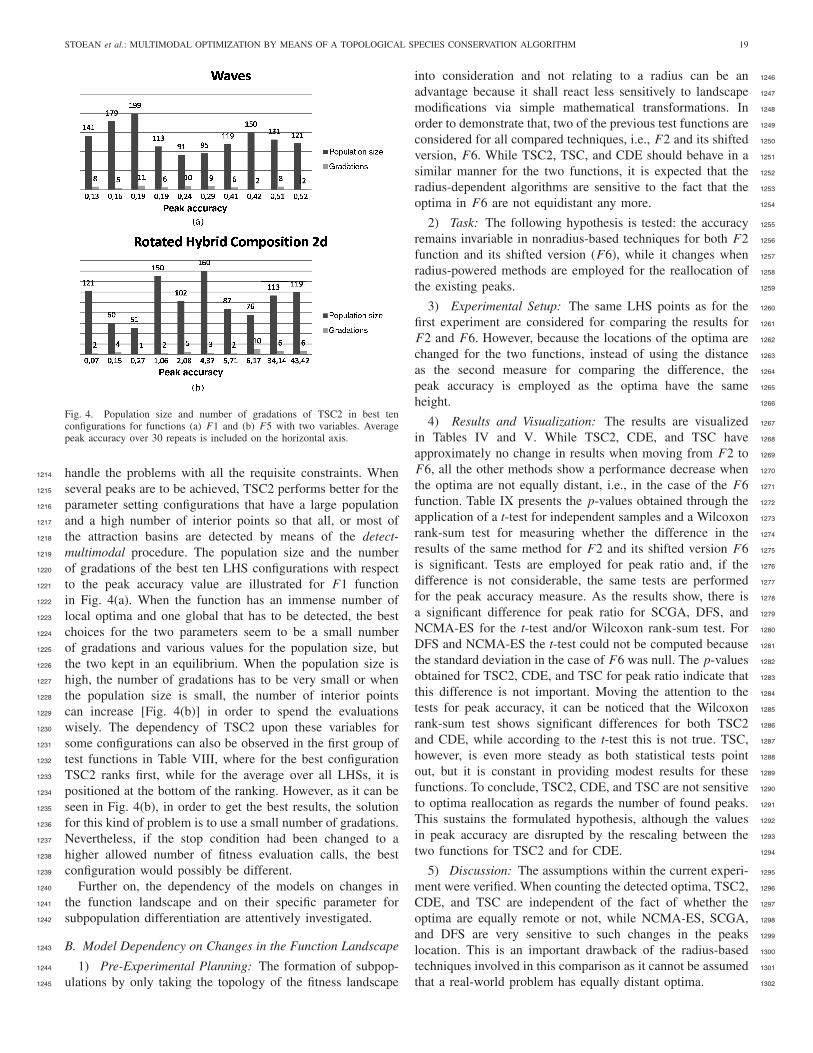
STOEAN et al.: MULTIMODAL OPTIMIZATION BY MEANS OF A TOPOLOGICAL SPECIES CONSERVATION ALGORITHM 19

Fig. 4. Population size and number of gradations of TSC2 in best tenconfigurations for functions (a) F1 and (b) F5 with two variables. Averagepeak accuracy over 30 repeats is included on the horizontal axis.

handle the problems with all the requisite constraints. When1214

several peaks are to be achieved, TSC2 performs better for the1215

parameter setting configurations that have a large population1216

and a high number of interior points so that all, or most of1217

the attraction basins are detected by means of the detect-1218

multimodal procedure. The population size and the number1219

of gradations of the best ten LHS configurations with respect1220

to the peak accuracy value are illustrated for F1 function1221

in Fig. 4(a). When the function has an immense number of1222

local optima and one global that has to be detected, the best1223

choices for the two parameters seem to be a small number1224

of gradations and various values for the population size, but1225

the two kept in an equilibrium. When the population size is1226

high, the number of gradations has to be very small or when1227

the population size is small, the number of interior points1228

can increase [Fig. 4(b)] in order to spend the evaluations1229

wisely. The dependency of TSC2 upon these variables for1230

some configurations can also be observed in the first group of1231

test functions in Table VIII, where for the best configuration1232

TSC2 ranks first, while for the average over all LHSs, it is1233

positioned at the bottom of the ranking. However, as it can be1234

seen in Fig. 4(b), in order to get the best results, the solution1235

for this kind of problem is to use a small number of gradations.1236

Nevertheless, if the stop condition had been changed to a1237

higher allowed number of fitness evaluation calls, the best1238

configuration would possibly be different.1239

Further on, the dependency of the models on changes in1240

the function landscape and on their specific parameter for1241

subpopulation differentiation are attentively investigated.1242

B. Model Dependency on Changes in the Function Landscape1243

1) Pre-Experimental Planning: The formation of subpop-1244

ulations by only taking the topology of the fitness landscape1245

into consideration and not relating to a radius can be an 1246

advantage because it shall react less sensitively to landscape 1247

modifications via simple mathematical transformations. In 1248

order to demonstrate that, two of the previous test functions are 1249

considered for all compared techniques, i.e., F2 and its shifted 1250

version, F6. While TSC2, TSC, and CDE should behave in a 1251

similar manner for the two functions, it is expected that the 1252

radius-dependent algorithms are sensitive to the fact that the 1253

optima in F6 are not equidistant any more. 1254

2) Task: The following hypothesis is tested: the accuracy 1255

remains invariable in nonradius-based techniques for both F2 1256

function and its shifted version (F6), while it changes when 1257

radius-powered methods are employed for the reallocation of 1258

the existing peaks. 1259

3) Experimental Setup: The same LHS points as for the 1260

first experiment are considered for comparing the results for 1261

F2 and F6. However, because the locations of the optima are 1262

changed for the two functions, instead of using the distance 1263

as the second measure for comparing the difference, the 1264

peak accuracy is employed as the optima have the same 1265

height. 1266

4) Results and Visualization: The results are visualized 1267

in Tables IV and V. While TSC2, CDE, and TSC have 1268

approximately no change in results when moving from F2 to 1269

F6, all the other methods show a performance decrease when 1270

the optima are not equally distant, i.e., in the case of the F6 1271

function. Table IX presents the p-values obtained through the 1272

application of a t-test for independent samples and a Wilcoxon 1273

rank-sum test for measuring whether the difference in the 1274

results of the same method for F2 and its shifted version F6 1275

is significant. Tests are employed for peak ratio and, if the 1276

difference is not considerable, the same tests are performed 1277

for the peak accuracy measure. As the results show, there is 1278

a significant difference for peak ratio for SCGA, DFS, and 1279

NCMA-ES for the t-test and/or Wilcoxon rank-sum test. For 1280

DFS and NCMA-ES the t-test could not be computed because 1281

the standard deviation in the case of F6 was null. The p-values 1282

obtained for TSC2, CDE, and TSC for peak ratio indicate that 1283

this difference is not important. Moving the attention to the 1284

tests for peak accuracy, it can be noticed that the Wilcoxon 1285

rank-sum test shows significant differences for both TSC2 1286

and CDE, while according to the t-test this is not true. TSC, 1287

however, is even more steady as both statistical tests point 1288

out, but it is constant in providing modest results for these 1289

functions. To conclude, TSC2, CDE, and TSC are not sensitive 1290

to optima reallocation as regards the number of found peaks. 1291

This sustains the formulated hypothesis, although the values 1292

in peak accuracy are disrupted by the rescaling between the 1293

two functions for TSC2 and for CDE. 1294

5) Discussion: The assumptions within the current experi- 1295

ment were verified. When counting the detected optima, TSC2, 1296

CDE, and TSC are independent of the fact of whether the 1297

optima are equally remote or not, while NCMA-ES, SCGA, 1298

and DFS are very sensitive to such changes in the peaks 1299

location. This is an important drawback of the radius-based 1300

techniques involved in this comparison as it cannot be assumed 1301

that a real-world problem has equally distant optima. 1302

20 IEEE TRANSACTIONS ON EVOLUTIONARY COMPUTATION

Fig. 5. Average number of optima in 30 repeats that are detected for the Waves function (F1) for different radius values within (a) SCGA, (b) DFS, and(c) NCMA-ES. The distinct values for the number of gradations in TSC2 and the amount of detected optima are represented in (d).

C. Model Dependency on Niche Radius or Number of Grada-1303

tions Parameters1304

1) Pre-Experimental Planning: As radius-based tech-1305

niques ranked below the other methods for the asymmetric1306

function F1 in the first experiment, finding a proper value1307

for the radius and subsequently investigating how dependent1308

these methods are on the values of this parameter is of great1309

interest. Plus, the reliance of TSC2 to the number of gradations1310

parameter is also of major concern.1311

2) Task: Investigate how sensitive TSC2, on the one hand,1312

and the radius-based methods, on the other hand, are on1313

the specific parameters for determining multimodality, i.e.,1314

number of gradations and radius, respectively. Different values1315

are tried for the radius/number of gradations on the F1 test1316

function. The hypothesis to be tested is the following: TSC21317

is not as sensitive to the changes in the values of the number1318

of gradations parameter as SCGA, DFS, and NCMA-ES are1319

to the variations in their corresponding radius parameter when1320

optimizing a function with many peaks.1321

3) Experimental Setup: In order to find the best values for1322

the radius/number of gradations when tackling the F1 func-1323

tion, the best LHS configuration found in the first experiment1324

is used for all the parameters, except the two examined ones.1325

For each configuration, 30 repeats are performed. While for1326

TSC2, the number of gradations is tried for all possible values1327

considered in the direct comparison experiment (1–15), for the1328

others, the radius is exponentially scaled. The starting value is1329

computed using the Deb and Goldberg formula (1) and then1330

the value is multiplied with integer powers of 2 taken from1331

the interval {−7, −6, . . . , 6, 7}.1332

4) Results and Visualization: Results obtained for F1 by1333

SCGA, DFS, and NCMA-ES with different values for the1334

radius parameter are shown in Fig. 5(a)–(c). The actual value1335

found using Deb and Goldberg formula is approximately 0.5. 1336

It can be noticed, however, from the SCGA and NCMA-ES 1337

graphics that the best average result is not obtained for this 1338

value, but for smaller ones, to be more specific, for 0.126 and 1339

0.25, respectively. Nevertheless, for DFS, the best configura- 1340

tion was precisely the one that had the radius computed by 1341

Deb and Goldberg formula, but the method could only reach 1342

a modest result, that is 3.8 peaks in average. None of the 1343

values generated for the radius was proper for detecting all 10 1344

optima of the function through the three methods. Moreover, 1345

when the value for the radius is higher than 1, the number of 1346

detected optima decreases to only approximately one solution. 1347

Fig. 5(d) outlines the average number of detected optima 1348

when trying different values for the number of gradations 1349

parameter within TSC2. As it can be seen, by increasing the 1350

value of the number of gradations from 2 up to 13, more than 1351

9.6 optima are detected in average for 30 runs of the same 1352

configuration. The results shown in the four figures indicate 1353

that the tested hypothesis is correct. 1354

Finally, as a distinct reinforcement of the validity of the 1355

given hypothesis, Fig. 6 illustrates the parameters influence 1356

on performance (in terms of found peaks) of the same SCGA, 1357

DFS, NCMA-ES, and TSC2 methods on problem F1. The 1358

visualization method divides the measured 30 LHS configu- 1359

rations into three equally sized groups, i.e., a good, middle, 1360

and a badly performing set. Instead of a usual box plot bar, an 1361

approximated percentile depiction is chosen as it emphasizes 1362

more where the single points are located. The dot in the middle 1363

of each bar represents the average (in parameter values of 1364

this group), the largest vertical line stands for the median, 1365

while the others represent the hinges. As it can be seen in 1366

the Fig. 6(a) and (b), the only parameter that has a great 1367

influence over the results for SCGA and DFS is the radius, 1368

which is set in average around 1 for the best 10 configurations, 1369

STOEAN et al.: MULTIMODAL OPTIMIZATION BY MEANS OF A TOPOLOGICAL SPECIES CONSERVATION ALGORITHM 21

Fig. 6. Box percentile plots of LHS (30) parameters for (a) SCGA, (b) DFS, (c) NCMA-ES, and (d) TSC2 on the Waves function (F1). Note that the threequality groups reflect relative and not absolute quality (in terms of best and worst).

while for the second 10 configurations it is moved to 3 and1370

the worst 10 configurations had it with the greatest value,1371

that is approximately 4. For NCMA-ES, the radius parameter1372

still remains important, however, its significance is not of1373

the same magnitude, as it allows other parameters to matter.1374

The niche parameter is also taken around 15 for the best1375

10 configurations and the results get worse when its value1376

decreases. The important parameters for TSC2 are the size1377

of the population and the mutation strength and the best1378

results are achieved when the former is high and the latter1379

is low. The number of gradations is not relevant for this1380

test case, fact that also sustains the conclusions derived from1381

Fig. 5. To conclude, in Fig. 6, apart from a visualization1382

of the other parameters weight on the peak accuracy, the1383

variability of the radius value as opposed to the consistency of1384

the number of gradations once more supports the formulated1385

hypothesis.1386

5) Discussion: It can be noticed that TSC2 does not very 1387

much depend on the value that is chosen for the number of 1388

gradations parameter, while the picking of the right value for 1389

the radius parameter within SCGA, DFS, and NCMA-ES is 1390

vital in obtaining good results. Figs. 5 and 6 also show this, 1391

the former taking into account the best configuration averaged 1392

over several repeats, while the latter considering only relative 1393

performance values and not the absolute ones for one tested 1394

algorithm. It may be argued that adjusting the radius by the 1395

use of a metaheuristic would be the trivial solution to the 1396

problem of setting its value. However, if the various attraction 1397

basins have unequal sizes, a unique value for the radius to 1398

differentiate between species connected to each peak cannot 1399

be appointed. Plus, this would add complexity to the respective 1400

technique, while the proposed TCS2 approach is not sensitive 1401

to an otherwise easy to calibrate corresponding value for the 1402

number of gradations. 1403

22 IEEE TRANSACTIONS ON EVOLUTIONARY COMPUTATION

V. Conclusion1404

In this paper, a multimodal evolutionary technique deriving1405

from an earlier integration of concepts of two modern methods1406

was further augmented by imposing several control variables,1407

supporting diversity and aiming for a prolonged search time1408

by inherently saving fitness evaluations. The novel TSC2 was1409

tested for the optimization of several benchmark functions and1410

a real-world instance. To justify its development, results were1411

directly compared to the original TSC version [14] and the1412

better one of the parent techniques, the SCGA [6]. To be even1413

more critical, experiments were further performed in contrast1414

to one related, recent evolutionary multimodal approach, the1415

DFS [7], to another competitive radius-based methodology, the1416

NCMA-ES [15] and, finally, to a complementary method of1417

crowding differential evolution (CDE) [11].1418

TSC2 aimed to inherit the strengths from SCGA and the1419

manner of detecting multimodality within the MGA [5], while1420

avoiding their shortcomings and going beyond the initial TSC1421

combination in the construction of a more robust algorithm,1422

able to deal with real-valued multimodal optimization prob-1423

lems. In the first respect:1424

1) the fitness landscape-triggered methodology obsoletes1425

the use of the radius threshold for species differentiation;1426

2) the sizes of the species are thus directly correlated1427

with those of the basins to which they are connected,1428

as they flexibly adapt to the shape of the landscape.1429

Therefore, the species are not forced to be formed within1430

equally spaced hyperspheres that depend on the value of1431

a threshold, as it is the case in radius-based evolutionary1432

approaches;1433

3) the preservation of the most prolific individuals within1434

each subpopulation takes place in order to maintain the1435

spread of the potential solutions over the search space;1436

4) a manner of keeping track of all individuals species is1437

proposed in order to reduce the expenses regarding the1438

amount of consumed fitness evaluations.1439

In the second regard, the extensions of TSC2 above the1440

previous TSC targeted the following.1441

1) For the purpose of further carefully saving fitness1442

calls and thus of an extension of evolutionary time,1443

a notion of similarity is employed when possible, in-1444

stead of repeatedly referring the detect − multimodal1445

procedure.1446

2) Exploration is increased by broadening the opportunities1447

for new diverse species as a result of reproduction.1448

3) The species seeds are not directly copied into the popula-1449

tion of the next generation, but their possible redundancy1450

is checked and prevented beforehand.1451

4) A fixed upper bound for the number of seeds to record is1452

set, in order to avoid the whole population of individuals1453

turning into prototypes for an overestimated number of1454

species.1455

Experiments show that the new TSC2 technique achieves1456

both liberation from a crucial parameter and significantly1457

better performance than the algorithms it is compared1458

to, especially for the test functions that have an irregular1459

landscape representation. Additionally, the results of the1460

expansions on top of the preliminary TSC argued in favor of 1461

the new TSC2 approach. 1462

From a practical perspective, the results on the traditional 1463

benchmark problems bring evidence of the type of real-world 1464

problems that can reach solution by means of TSC2. Although 1465

many 2-D functions are employed for testing purposes, the 1466

experiments specifically answered 10 to 20-D tasks as a 1467

reasonable model substitute for real instances. Moreover, cases 1468

of higher multimodality (as usual in practice), ranging from 1469

10 to 20 important optima to be found, were additionally 1470

successfully solved. Very importantly, all these specific as- 1471

signments are resolved with a relatively small budget of 1472

fitness evaluations (30 000), which is a primary concern in 1473

real applications. Finally, TSC2 has been shown to deal well 1474

with asymmetric landscapes that can be expected for many 1475

real-world applications. 1476

A first step to extend the current work would be to 1477

add mutation step size adaptation mechanisms, as this will 1478

surely open a path leading to substantially increased perfor- 1479

mance. 1480

Secondly, for a complete and general multimodal instru- 1481

ment, it would be interesting to study and further tailor the 1482

proposed approach in application to problems of dynamic na- 1483

ture. Since the landscape changes over time, the topologically- 1484

triggered TSC2 flexibility in subpopulation formation should 1485

deal with this situation in a useful manner. 1486

Another task that is currently under development is the 1487

enhancement of a tool for estimating the number of lo- 1488

cal/global optima within the landscape of a function [29], this 1489

time by taking advantage of the novel features within TSC2. 1490

Knowing this information in advance can be very valuable for 1491

a technique dealing with a specific problem. It can help in 1492

setting the proper values for parameters or even in deciding 1493

the method that should be employed for solving the task. TSC2 1494

represents a good inspiration for this purpose as it keeps track 1495

of all the different detected peaks through direct landscape 1496

inspection and it would help to estimate how many niches 1497

exist in the search space from the very early stages of the 1498

evolutionary process. 1499

References 1500

[1] A. E. Eiben and J. E. Smith, Introduction to Evolutionary Computing. 1501

Berlin, Germany: Springer-Verlag, 2003. AQ:31502

[2] M. Preuss, L. Schonemann, and M. Emmerich, “Counteracting genetic 1503

drift and disruptive recombination in (µ+/, λ)-EA on multimodal fitness 1504

landscapes,” in Proc. Genetic Evol. Comput. Conf. (GECCO), vol. 1. 1505

2005, pp. 865–872. 1506

[3] K. A. DeJong, “An analysis of the behavior of a class of genetic 1507

adaptive systems,” Ph.D. dissertation, Dept. Comput. Commun. Sci., 1508

Univ. Michigan, Ann Arbor, 1975. 1509

[4] D. E. Goldberg and J. Richardson, “Genetic algorithms with sharing for 1510

multimodal function optimization,” in Proc. Genetic Algorithms Their 1511

Applicat. Conf., 1987, pp. 41–49. 1512

[5] R. K. Ursem, “Multinational evolutionary algorithms,” in Proc. Congr. 1513

Evol. Comput. (CEC), vol. 3. 1999, pp. 1633–1640. 1514

[6] J. P. Li, M. E. Balazs, G. T. Parks, and P. J. Clarkson, “A species 1515

conserving genetic algorithm for multimodal function optimization,” 1516

Evol. Comput., vol. 10, no. 3, pp. 207–234, 2002. 1517

[7] A. D. Cioppa, C. D. Stefano, and A. Marcelli, “Where are the niches? 1518

Dynamic fitness sharing,” IEEE Trans. Evol. Comput., vol. 11, no. 4, 1519

pp. 453–465, Aug. 2007. 1520

STOEAN et al.: MULTIMODAL OPTIMIZATION BY MEANS OF A TOPOLOGICAL SPECIES CONSERVATION ALGORITHM 23

[8] J. H. Holland, Adaptation in Natural and Artificial Systems. Ann Arbor,1521

MI: Univ. of Michigan Press, 1975.1522

[9] D. J. Cavicchio, “Adaptive search using simulated evolution,” Ph.D.1523

dissertation, Dept. Comput. Commun. Sci., Univ. Michigan, Ann Arbor,1524

1970.1525

[10] O. M. Shir and T. Back, “Niching with derandomized evolution strate-1526

gies in artificial and real-world landscapes,” Natural Comput.: Int. J.,1527

vol. 8, no. 1, pp. 171–196, Mar. 2009.AQ:4 1528

[11] R. Thomsen, “Multimodal optimization using crowding-based differen-1529

tial evolution,” in Proc. Congr. Evol. Comput. (CEC), vol. 2. 2004, pp.1530

1382–1389.1531

[12] K. Deb and D. E. Goldberg, “An investigation of niche and species1532

formation in genetic function optimization,” in Proc. 3rd Int. Conf.1533

Genetic Algorithms, 1989, pp. 42–50.1534

[13] R. K. Ursem, “Multinational gas: Multimodal optimization techniques1535

in dynamic environments,” in Proc. Genetic Evol. Comput. Conf.1536

(GECCO), vol. 1. 2000, pp. 19–26.1537

[14] C. Stoean, M. Preuss, R. Stoean, and D. Dumitrescu, “Disburdening the1538

species conservation evolutionary algorithm of arguing with radii,” in1539

Proc. Genetic Evol. Comput. Conf. (GECCO), 2007, pp. 1420–1427.1540

[15] O. M. Shir and T. Baeck, “Niche radius adaptation in the CMA-ES1541

niching algorithm,” in Proc. Parallel Problem Solving Nature (PPSN),1542

LNCS 4193. 2006, pp. 142–151.1543

[16] N. Hansen and A. Ostermeier, “Completely derandomized self-1544

adaptation in evolution strategies,” Evol. Comput., vol. 9, no. 2, pp.1545

159–195, Jun. 2001.1546

[17] O. Shir and T. Back, “Niching in evolution strategies,” in Proc. Genetic1547

Evol. Comput. Conf. (GECCO), 2005, pp. 915–916.1548

[18] C. Igel, T. Suttorp, and N. Hansen, “A computational efficient covariance1549

matrix update and a (1+1)-CMA for evolution strategies,” in Proc.1550

Genetic Evol. Comput. Conf. (GECCO), 2006, pp. 453–460.1551

[19] N. Hansen, “The CMA evolution strategy: A tutorial,” Jan. 18, 20091552

[Online]. Available: http://www.lri.fr/∼hansen/cmatutorial.pdf1553

[20] S. W. Mahfound, “Niching methods for genetic algorithms,” Genetic1554

Algorithms Lab., Univ. Illinois, Urbana-Champaign, Tech. Rep. 95 001,1555

1995.1556

[21] O. J. Mengshoel and D. E. Goldberg, “Probability crowding: Determin-1557

ing crowding with probabilistic replacement,” in Proc. Genetic Evol.1558

Comput. Conf. (GECCO), 1999, pp. 409–416.1559

[22] R. G. Reynolds and W. Sverdlik, “Problem solving using cultural1560

algorithms,” in Proc. Int. Conf. Evol. Comput. (CEC), vol. 1. 1994, pp.1561

645–650.1562

[23] J. Alami, L. Benameur, and A. Imrani, “Fuzzy clustering based parallel1563

cultural algorithm,” Int. J. Soft Comput., vol. 2, no. 4, pp. 562–571,1564

2007.1565

[24] M. Preuss, “Niching prospects,” in Proc. Bioinspired Optim. Methods1566

Their Applicat. (BIOMA), Jozef Stefan Institute, Ljubljana, Slovenia,1567

2006, pp. 25–34.1568

[25] P. N. Suganthan, N. Hansen, J. J. Liang, K. Deb, Y.-P. Chen, A. Auger,1569

and S. Tiwari, “Problem definition and evaluation criteria for the1570

CEC 2005 special session on real-parameter optimization,” Nanyang1571

Technological University, Singapore, Tech. Rep., 2005.AQ:5 1572

[26] V. Feoktistov, Differential Evolution: In Search of Solutions. Berlin,1573

Germany: Springer-Verlag, 2006.1574

[27] D. C. Montgomery, Design and Analysis of Experiments, 5th ed. New1575

York: Wiley, 2001.1576

[28] T. Bartz-Beielstein, Experimental Research in Evolutionary Computa-1577

tion: The New Experimentalism (Natural Computing Series). Berlin:1578

Springer, 2006.1579

[29] C. Stoean, M. Preuss, R. Stoean, and D. Dumitrescu, “EA-powered basin1580

number estimation by means of preservation and exploration,” in Proc.1581

10th Int. Conf. Parallel Problem Solving Nature (PPSN), LNCS 5199.1582

2008, pp. 569–578.1583

Catalin Stoean (M’08) was born in Craiova,1584

Romania, on August 31, 1979. He received the M.S.1585

degree from the University of Craiova, Craiova,AQ:6 1586

Romania, and the Ph.D. degree from the Babes-1587

Bolyai University, Cluj-Napoca, Romania, both in1588

computer science, in 2003 and 2008, respectively.1589

Since 2003, he has been an Assistant Professor1590

at the Department of Computer Science, Faculty of1591

Mathematics and Computer Science, University of1592

Craiova. For the last couple of years, he has been1593

lecturing on the topic of artificial intelligence. He has1594

been active in the fields of evolutionary computation and machine learning. He AQ:71595

has been a Visiting Scholar of the University of Dortmund and the University 1596

of Cologne, Germany, courtesy of two grants from the German Academic 1597

Exchange Service. 1598

Dr. Stoean is a Member of the IEEE Computer Society. In 2008, he was part 1599

of a group of four people who won the 2008 Romanian Academy Grigore 1600

Moisil Award for computer science research conducted in 2006. 1601

Mike Preuss (M’08) was born in Ahlen/Westfalen, 1602

Germany, on March 23, 1969. He received the 1603

Diploma degree from the Department of Com- AQ:81604

puter Science, Dortmund University of Technology, 1605

Dortmund, Germany, in 1998. 1606

Since 2000, he has been a Research Associate with 1607

the Department of Computer Science, Dortmund 1608

University of Technology. His mission is to further 1609

develop the experimental methodology for nondeter- 1610

ministic optimization algorithms by means of tuning, 1611

adaptability measures, and other experimental anal- 1612

ysis techniques. These are essential for the design of specific evolutionary 1613

algorithms (EA)-based algorithms for industrial optimization in various engi- 1614

neering domains, e.g., thermodynamics and ship propulsion technology. His 1615

research interests include the field of EA for real-valued problems, namely 1616

for multimodal and multiobjective niching. 1617

Prof. Preuss is active in designing authentic artificial intelligence compo- AQ:91618

nents for believable opponents and increased player satisfaction as a member 1619

of the IEEE Computational Intelligence Society (CIS) Games Technical 1620

Committee and the Chair of the CIS task force on realtime strategy games. 1621

Ruxandra Stoean (M’08) was born in Craiova, 1622

Romania, on August 2, 1979. She received the M.S. 1623

degree from the University of Craiova, Craiova, 1624

Romania, and the Ph.D. degree from the Babes- 1625

Bolyai University, Cluj-Napoca, Romania, both in 1626

computer science, in 2003 and 2008, respectively. 1627

She is currently an Assistant Professor with the 1628

Department of Computer Science, Faculty of Mathe- 1629

matics and Computer Science, University of Craiova, 1630

where she lectures on nonprocedural programming 1631

and laboratories of artificial intelligence and logic AQ:101632

programming. Her current research interests include support vector machines, 1633

evolutionary computation, and data mining. She has been the guest of the 1634

Universities of Cologne and Dortmund, Germany, with the support of a 1635

German Academic Exchange Service grant. 1636

Dr. Stoean was awarded a 2008 Computer Science Prize from the Romanian 1637

Academy for a collection of papers in evolutionary computation as part of a 1638

four-person group. She is a member of the IEEE Computer Society. 1639

D. Dumitrescu received the M.S. and Ph.D. AQ:111640

degrees from Babes-Bolyai University, Cluj-Napoca, 1641

Romania. AQ:121642

He is currently a Professor with the Department 1643

of Computer Science, Babes-Bolyai University. His AQ:131644

current research interests include natural computing, 1645

complexity, and computational game theory. 1646

1647