A Selection Framework for LHCb's ... - CERN Document Server
139
Dissertation zur Erlangung des akademischen Grades Dr. rer. nat. A Selection Framework for LHCb’s Upgrade Trigger Niklas Nolte geboren in Hildesheim, 1994 2020 Lehrstuhl für Experimentelle Physik V Fakultät Physik Technische Universität Dortmund CERN-THESIS-2020-331 22/02/2021
-
Upload
khangminh22 -
Category
Documents
-
view
1 -
download
0
Transcript of A Selection Framework for LHCb's ... - CERN Document Server

Dissertation zur Erlangung des akademischenGrades
Dr. rer. nat.
A Selection Framework for LHCb’sUpgrade Trigger
Niklas Noltegeboren in Hildesheim, 1994
2020
Lehrstuhl für Experimentelle Physik VFakultät Physik
Technische Universität Dortmund
CER
N-T
HES
IS-2
020-
331
22/0
2/20
21

Erstgutachter: Prof. Dr. Johannes AlbrechtZweitgutachter: Dr. Johannes ErdmannAbgabedatum: 17. Dezember 2020

Kurzfassung
Das LHCb Experiment am Large Hadron Collier am CERN wird momentan für dienächste Datennahme verändert und modernisiert. Die instantane Luminosität wirdum einen Faktor fünf erhöht, damit mehr Daten in kürzerer Zeit aufgenommenwerden können. Die erste Stufe der Datennahme, der Hardwaretrigger, wirdentfernt. LHCb muss nun eine Kollisionsrate von 30 MHz in Echtzeit verarbeiten.In dieser Arbeit werden drei Projekte vorgestellt, die signifikant zu der Entwicklungeines schnellen und effizienten Triggersystems beitragen.
Der erste Beitrag ist ein Scheduling Algorithmus mit vernachlässigbarem Overheadin der neuen Trigger-Applikation. Der Algorithmus steuert das Multi-Threadingdes Systems und ist der erste Algorithmus in LHCb, der den technischen Spezifika-tionen des Systems genügt. Durch die Restriktion auf Inter-Event Parallelismuskönnen die meisten teuren Entscheidungen schon vor der Laufzeit der Applikationgetroffen werden.
Der zweite Beitrag besteht aus mehreren Algorithmen zur Filterung und Kombina-tion von Teilchen in der Kollision. Diese Algorithmen sind bis zu mehrerenGrößenordnungen schneller als die aktuellen, etablierten Algorithmen. DerEinsatz der neuen Algorithmen in der zweiten Trigger-Phase (HLT2) ist einwichtiger Schritt zur Vervollständigung eines Trigger-Systems, dass den erhöhtenAnforderungen entspricht.
Das letzte Projekt beschäftigt sich mit der Bandbreite, mit der der TriggerKollisionen abspeichert. Dazu wird die wichtigste Selektion im HLT2 betrachtet,der topologische Trigger. Dieser Trigger versucht, Zerfälle von beauty Hadroneninklusiv zu selektieren. Zuerst wird der Selektionsalgorithmus selber optimiert.In einem zweiten Schritt werden die Kollisionen, die der Selektion entsprechen,getrimmt. Irrelevante Information für die Analyse von beauty Hadronen indiesen Kollisionen werden entfernt. Damit kann die Bandbreite pro gespeicherterKollision verringert werden.
iii

Abstract
The LHCb experiment at the Large Hadron Collider at CERN is planning a majordetector upgrade for the next data taking period. The instantaneous luminosityis increased by a factor of five to generate more data per time. The hardwaretrigger stage preceding detector readout is removed and LHCb now has to process30 MHz of incoming events in real time. The work presented in this thesis showsthree contributions towards a fast and efficient trigger system.
The first contribution is a multi-threaded scheduling algorithm to work withnegligible overhead in the Upgrade regime. It is the first implementation forLHCb capable of realizing arbitrary control and data flow at the required speed.It restricts itself to inter-event concurrency to avoid costly runtime schedulingdecisions.
The second contribution comprises several algorithms to perform particle combi-nation, vertexing and selection steps in the second HLT stage. These algorithmsshow competitive performances which can speed up the selection stage of HLT2by orders of magnitude. Employing these algorithms marks a significant steptowards an HLT2 application fast enough for the increased event rate.
The third contribution concerns the most important and most costly HLT2selection at LHCb, the Topological Trigger. It aims to inclusively capture manybeauty-flavored decay chains. First, the algorithm for event selection is optimized.In a second step, output bandwidth is reduced significantly by employing aclassification algorithm for selecting additional relevant information present inthe event.
iv

Contents
1 Introduction 1
2 The Standard Model of Particle Physics 42.1 Obtaining a solution to unsolved problems with LHCb . . . . . . 6
3 The LHCb Detector at the LHC 83.1 The Large Hadron Collider . . . . . . . . . . . . . . . . . . . . . . 83.2 The LHCb detector . . . . . . . . . . . . . . . . . . . . . . . . . . 11
3.2.1 The tracking system . . . . . . . . . . . . . . . . . . . . . 12The Vertex Locator . . . . . . . . . . . . . . . . . . . . . 13The Upstream Tracker . . . . . . . . . . . . . . . . . . . . 14The magnet . . . . . . . . . . . . . . . . . . . . . . . . . . 15The SciFi tracker . . . . . . . . . . . . . . . . . . . . . . . 15Track types in LHCb reconstruction . . . . . . . . . . . . 16
3.2.2 The particle identification system . . . . . . . . . . . . . . 17The Ring Imaging Cherenkov Detectors . . . . . . . . . . 17Electromagnetic and hadronic calorimeters . . . . . . . . . 18The muon stations . . . . . . . . . . . . . . . . . . . . . . 19
3.2.3 An overview over the LHCb software . . . . . . . . . . . . 193.3 LHCb beauty and charm decay topology . . . . . . . . . . . . . . 21
4 The LHCb Upgrade Trigger 234.1 Why upgrade to a full software trigger? . . . . . . . . . . . . . . . 234.2 Upgrade trigger workflow . . . . . . . . . . . . . . . . . . . . . . 27
4.2.1 The first High Level Trigger: HLT1 . . . . . . . . . . . . . 274.2.2 The disk buffer, alignment and calibration . . . . . . . . . 294.2.3 The second HLT stage . . . . . . . . . . . . . . . . . . . . 314.2.4 Building blocks for trigger software . . . . . . . . . . . . . 31
Configurability and the build model . . . . . . . . . . . . 32
v

Contents
4.3 Computing challenges in the Upgrade HLT . . . . . . . . . . . . . 324.3.1 Bandwidth requirements . . . . . . . . . . . . . . . . . . . 33
Selective persistence . . . . . . . . . . . . . . . . . . . . . 334.3.2 Throughput requirements . . . . . . . . . . . . . . . . . . 34
5 Principles for High Performance Computing in the Trigger 375.1 Caching and predictability in CPUs . . . . . . . . . . . . . . . . . 375.2 Dynamic memory allocation . . . . . . . . . . . . . . . . . . . . . 395.3 Vectorization . . . . . . . . . . . . . . . . . . . . . . . . . . . . . 395.4 Multi-core utilization with multi-threading . . . . . . . . . . . . . 40
Gaudi::Functional . . . . . . . . . . . . . . . . . . . . . . 42
6 A Scheduling Algorithm for the Upgrade Trigger Regime 436.1 Control and data flow . . . . . . . . . . . . . . . . . . . . . . . . 436.2 The baseline: A multi-threaded event scheduler for Gaudi . . . . 446.3 A new scheduling application . . . . . . . . . . . . . . . . . . . . 46
6.3.1 From intra- to inter-event concurrency . . . . . . . . . . . 466.3.2 The high level workflow . . . . . . . . . . . . . . . . . . . 466.3.3 The trigger control flow anatomy . . . . . . . . . . . . . . 476.3.4 Representation of data flow . . . . . . . . . . . . . . . . . 49
6.4 Event loop preparation - Initialization . . . . . . . . . . . . . . . 506.5 The event loop - Runtime . . . . . . . . . . . . . . . . . . . . . . 53
6.5.1 Task packaging . . . . . . . . . . . . . . . . . . . . . . . . 536.5.2 Sequence execution . . . . . . . . . . . . . . . . . . . . . . 53
6.6 The control flow barrier - Sharing work . . . . . . . . . . . . . . . 546.7 Scheduler performance . . . . . . . . . . . . . . . . . . . . . . . . 576.8 Summary and outlook . . . . . . . . . . . . . . . . . . . . . . . . 57
7 Selections and Combinatorics in Upgrade HLT2 597.1 Selection algorithms in the trigger workflow . . . . . . . . . . . . 597.2 Runtime performance in status quo . . . . . . . . . . . . . . . . . 627.3 The baseline algorithms . . . . . . . . . . . . . . . . . . . . . . . 63
7.3.1 Filtering with LoKi . . . . . . . . . . . . . . . . . . . . . . 637.3.2 Basics of combining . . . . . . . . . . . . . . . . . . . . . 647.3.3 Workflow in the baseline combiner . . . . . . . . . . . . . 65
7.4 Improving upon the baseline with new selections . . . . . . . . . . 687.4.1 Combining with ThOr . . . . . . . . . . . . . . . . . . . . 71
7.5 A new particle model . . . . . . . . . . . . . . . . . . . . . . . . . 737.5.1 Data layouts and LHCb::Particle . . . . . . . . . . . . . . 73
vi

Contents
7.5.2 The SoA particle . . . . . . . . . . . . . . . . . . . . . . . 767.6 Filtering and combining with the SoA particle model . . . . . . . 79
7.6.1 A Combiner for the SoA Particle . . . . . . . . . . . . . . 80The algorithm logic . . . . . . . . . . . . . . . . . . . . . . 81Combining . . . . . . . . . . . . . . . . . . . . . . . . . . 82Vertexing . . . . . . . . . . . . . . . . . . . . . . . . . . . 83
7.6.2 Benchmarks on combining with the SoA Particle . . . . . 837.7 Conclusion and Outlook . . . . . . . . . . . . . . . . . . . . . . . 84
8 The Topological Trigger with Selective Persistence 868.1 Input data . . . . . . . . . . . . . . . . . . . . . . . . . . . . . . . 878.2 Optimization of the topological event selection . . . . . . . . . . . 88
8.2.1 The metric for optimization: Trigger On Signal efficiency . 898.2.2 Topo candidate combination . . . . . . . . . . . . . . . . . 908.2.3 Boosted tree ensembles . . . . . . . . . . . . . . . . . . . . 938.2.4 Topological classification - Baseline comparison . . . . . . 958.2.5 Topological classification - Full input data . . . . . . . . . 100
8.3 Selective Persistence in the topological trigger . . . . . . . . . . . 105Selection based on primary vertex relations . . . . . . . . 106Selection based on trained classification . . . . . . . . . . 107
8.4 Summary and outlook . . . . . . . . . . . . . . . . . . . . . . . . 115
9 Conclusion 117
A Appendix 120A.1 Description of HLT1 trigger lines . . . . . . . . . . . . . . . . . . 120A.2 Additional information on input samples for the Topo . . . . . . . 122
Bibliography 123
vii

viii

1 Introduction
In Geneva, Switzerland, the European Organization for Nuclear Research (CERN)operates the largest ever built machine: The Large Hadron Collider (LHC) [1].This circular particle collider measures 26.7 km in circumference and collidesprotons and heavy ions at the TeV energy scale. At four distinct interaction pointsaround the perimeter, these collisions of unprecedented energy are captured byfour large detectors: ATLAS, CMS, ALICE and LHCb.
Until this day, these experiments have made countless measurements in fundamen-tal particle physics, including but not limited to the discovery of new particlesand precision measurements of particle properties and interactions. The mostimportant discovery was achieved in 2012 by the ATLAS and CMS collaborations:The Higgs-Boson [2, 3]. It is the last found elemental particle predicted by thebest tested fundamental physics theory, the Standard Model (SM) of particlephysics [4, 5, 6, 7].
Although the SM yields incredibly precise predictions all over the high energyphysics landscape, it fails to cover several observed phenomena of our universe,like the existence of dark matter [8] or the asymmetry of matter and antimatter[9, 10]. There is also no description of gravity included in the Standard Model.We must therefore conclude that the SM is, at best, an incomplete model of theinteractions in fundamental physics.
With steadily increasing energies and collision rates, experiments at the LHC tryto find hints for physics Beyond the Standard Model (BSM) in the vast amount ofdata they generate. Every measurement gives rise to new theories and discouragesothers. The LHCb detector, which is in the focus of this thesis, specializes inindirect searches for BSM physics in beauty and charm decay processes. Around1000 engineers and physicists collaborate to operate this detector, to process thedata and to analyze it.
As the LHC is currently in the second long shutdown LS 2, LHCb is undergoinga major detector upgrade to prepare for a fivefold increase in luminosity in thethird Run of the LHC. Major changes include a new tracking system and a full
1
1 Introduction
replacement of all readout electronics. Most importantly for this thesis, the LHCbtrigger system is being reworked completely [11].A trigger system acts as filter for the huge amount of incoming data, as wecannot afford to persist multiple terabytes per second of collision information. Itreconstructs particles trajectories in different detector components and ultimatelycombines them to form decay and collision vertices. To find the interesting physicsneedle in the haystack of interactions that a high energy hadronic collision creates,one can impose requirements on particle trajectories and vertices.
Until the end of Run 2 in 2018, the first selection step was performed by a hardwaretrigger, L0, that filtered events with a rate of 1 MHz. The two subsequent HighLevel Trigger (HLT) software stages thus had to operate at a much lower ratethan the nominal LHC collision rate.From 2021 onwards, there will not be a hardware trigger stage in LHCb’s dataprocessing flow to achieve a higher amount of flexibility and efficiency. This posessignificant challenges to the HLT processing farm, as it has to operate in realtime with a collision rate of 40 million per second. LHCb is the first of the fourbig experiments at the LHC to take the leap towards a software-only triggersystem. Together with the aforementioned fivefold increase of luminosity, thecomputational requirements on the HLT computing farm increase by about twoorders of magnitude with respect to previous data taking periods. In contrast tothese requirements, the allocated computing budget does not allow for a farmthat is orders of magnitude more powerful than the one that operated in 2018.
The second big challenge, next to computational load, is the limited outputbandwidth. The trigger needs to efficiently select physics signatures for allanalyses that researchers are interested in. Inclusive selections over such a broadrange of physics signatures results in large bandwidth outputs. Therefore, thesolution is made up by about 𝑂(103) exclusive selections built into the secondHLT stage. The fivefold increase of luminosity implies a fivefold increase ofinteresting data to be collected per unit of time, but also a similarly increasedlevel of noise. Selections need to be very pure to fit into the output bandwidthwhile not discarding too much interesting data. Significant efforts are being putinto the optimization of both HLT reconstruction and selection stages to meetboth timing and bandwidth requirements.
Some of these efforts are presented in this thesis. Chapter 2 introduces the SM andproblems that LHCb tries to gain further insight into. Chapters 3 and 4 discussthe upgrade LHCb detector and the upgrade trigger with its challenges in detail.
2

Chapter 5 takes a step back from the context of high energy physics to introduceprinciples for high performance computing on CPU architectures. Starting fromChapter 6, specific optimizations proposed for operation in the upgrade triggerare discussed. Chapter 6 describes the first feature complete implementationof a new scheduling algorithm to efficiently execute the HLT control flow withthousands of algorithms in online production. Chapter 7 is concerned with theimplementation of faster algorithms for performing physics selections and decaychain reconstruction. This work includes the introduction of a new data model forparticles. Finally, Chapter 8 tackles the output bandwidth problem by scrutinizingthe biggest bandwidth contributor, the Topological Beauty Trigger. It aims toinclusively select beauty decays based on kinematic and topological signaturesonly. With a subsequent classification algorithm, only essential data from theevent is filtered to save bandwidth without sacrificing efficiency.
3

2 The Standard Model of Particle Physics
The Standard Model of particle physics (SM) describes interaction dynamics ofelementary particles as a quantized field theory and is the best tested and verifiedparticle physics theory to this day. It is capable of modelling three out of the fourfundamental types of interactions, the electromagnetic, the strong and the weakforce. Gravity remains unaccounted for.
The collection of elementary particles within the SM comprise 12 fermions of halfinteger spin and 5 bosons of integer spin. We will henceforth imply the existence ofan antiparticle for each mentioned particle, exhibiting the same mass but invertedquantum numbers.
Six of the fermions are called quarks, which have third integer electric charge.There are up-type quarks (up, charm, top) which have a charge of +2/3 anddown-type (down, strange, bottom) quarks of charge −1/3. Quarks also carryanother quantum number called color.The other six fermions are called leptons, which are all colorless. Three of them(electron, muon, tau) have an electric charge of −1. The other three are calledneutrinos and they are electrically neutral. All fermionic elementary particleshave a common spin of 1/2.
The bosons act as mediator for the fundamental interactions. Photons are ex-changed during electromagnetic interaction, which couples to the electric charge.Quarks and charged leptons can interact electromagnetically.The 𝑊 ± and 𝑍0 bosons propagate the weak interaction, which couples to aquantum number called weak isospin. Only left-chiral particles and right-chiral an-tiparticles exhibit weak isospin. Chirality is an abstract concept of transformationbehavior that has a visual analogy for massless particles: Left-chiral means thatspin and momentum point in opposite directions, while for right-chiral particlesthey point to the same direction. This analogy cannot be made for massiveparticles, as their momentum depends on the observer frame. All particles caninteract under the weak force, given ”correct” chirality. Neutrinos, in fact, onlyinteract weakly.
4
The strong force couples to color and is mediated by eight different gluon states,which also carry color themselves. There are three colors and three anti-colors.All colors together make, in analogy to the additive color system, a colorless(or white) state, and so does a color with its anti-color. Because only colorlesssystems are stable in nature, we do not find quarks by themselves, but in boundstates called hadrons. The most common hadrons are 𝑞 ̄𝑞 states called Mesons,and 𝑞𝑞𝑞 states called baryons, but in principle all integer linear combinations of 𝑞 ̄𝑞and 𝑞𝑞𝑞 are possible. 𝑞𝑞 ̄𝑞 ̄𝑞 states called tetraquarks and 𝑞 ̄𝑞𝑞𝑞𝑞 called pentaquarkshave already been found in recent years [12, 13].The Higgs boson, found in 2012 [2, 3], is the only spin 0 elementary particle. It orig-inates the Higgs field, giving mass to all particles. A visual summary of elementalparticles and the interactions they take part in can be seen in Figure 2.1.
While the SM gives very accurate predictions and has been tested successfully overdecades, there are several phenomena besides gravity and general relativity thatit fails to explain. The SM predict massless neutrinos, but neutrino oscillationimplying a finite mass has been found around 2000 [14, 15, 16]. The NobelPrize was awarded for these findings in 2015. The observable matter-antimatterasymmetry [9, 10] or the existence of dark matter [8] in our universe are only afew examples of other unexplainable phenomena in the SM framework. Therefore,we must conclude that the SM is an incomplete model of the universe and mustbe overhauled or at least extended.
5

2 The Standard Model of Particle Physics
Figure 2.1: Elementary particles described within the Standard Model. Chargeis shown in green in the upper right corner of each box, color in red and spinin yellow at the lower right. A particles mass in eV is given at the left upperpart of the respective block. Modified from [17].
2.1 Obtaining a solution to unsolved problems withLHCb
With the help of collision experiments, physicists hope to find hints for physicsbeyond the Standard Model (BSM physics) that help to develop a model fit-ting these still unexplainable phenomena. The focus of this thesis, the LHCbexperiment, is one of these collision experiments. By colliding protons with highenergy and luminosity from the LHC, an unprecedented amount of beauty andcharm decays are recorded with the LHCb experiment. The current LHCb datasetcomprises about 𝑂(1011) beauty and 𝑂(1013) charm decays [18, 19, 20]. With
6

2.1 Obtaining a solution to unsolved problems with LHCb
data sets of such statistical power particle and decay properties can be measuredvery precisely. Measuring SM parameters helps in two ways. Deviations frompredicted values of these properties aid the invention of extensions to the SM andnew models. A measurement matching the prediction helps with the constraintand exclusion of other models.
Research within the LHCb collaboration focuses on different observable parameters.A prominent class of observables are those describing asymmetries under Charge-and Parity (CP) transformation. This is referred to as CP violation (CPV). CPVis predicted within the SM to a small degree, but additional sources of CPV arerequired to explain the matter-antimatter asymmetry [21]. Precise measurementsof CP observables are thus very valuable in the pursuit of explanations to theproblem. 𝐵0
𝑠 → 𝜙𝜙 and 𝐵0 → 𝐷+𝐷− are two examples of decays which aresensitive to parameters describing CP violation. CP measurements on these decaysare currently limited by statistical power of the analyzed dataset [22, 23].
A second interesting field of research in LHCb are searches for violation of chargedlepton flavor universality. The SM predicts a certain symmetry between leptonflavors. This implies that, up to differences induced by the lepton mass differences,branching fractions of decays involving charged leptons should not depend on thelepton flavor. However, LHCb published measurements that deviate from the SMwith 2-3 standard deviations significance [24, 25, 26, 27]. The uncertainties onmeasurements of lepton flavor universality depend on the statistical powers ofdatasets recording decays like 𝐵0 → 𝐾(∗)0𝑒+𝑒−, 𝐵0 → 𝐾(∗)0𝜇+𝜇−, 𝐵0 → 𝐷∗−𝜏+𝜈and 𝐵0 → 𝐷∗−𝜇+𝜈.
To decrease statistical uncertainties of all of these measurements, more data isneeded. During the current shutdown of the LHC, the experiment is upgraded tobe able to record new data at higher rates. The current LHCb dataset correspondsto an integrated luminosity of 9/fb. With the upgraded detector 50/fb shall berecorded within the next decade. The new data will be used to perform even moreprecise measurements and thus strengthen or negate recently found deviationsand constrain theoretical models even further.
7

3 The LHCb Detector at the LHC
Hints for physics beyond the Standard Model might be found in various niches ofphase space and it might be very hard to detect or very rare. The physicists’ bestguesses have traditionally been to inspect particle decays at higher and higherenergies to uncover new states, new particles and potentially new physics. Over thecourse of many decades, they have therefore built more and more powerful particlecolliders that operate at the highest possible energy. This chapter introduces theLarge Hadron Collider and the LHCb experiment, located at the CERN researchfacility. Note that the LHCb detector will be described in its envisioned stateafter the current upgrade.
3.1 The Large Hadron Collider
The result of striving towards higher energies ultimately led to the creation of theLarge Hadron Collider (LHC) [1], the largest ever built machine. It is a circularhadron collider operated by the European Organization for Nuclear Research(CERN) in Geneva, Switzerland. It measures 26.7 km in circumference, resides ina tunnel that is 50-175 m underground and accelerates protons and heavy ions to13 TeV and 5 TeV per nucleon, respectively. With such large energies, the LHCis able to create a unique environment for particle decays. While these and evenhigher energies can also be observed from cosmic particles, a particle collider hasthe advantage of a controlled environment. 1011 protons per bunch and 40 millionbunch crossing per second generated by two oppositely accelerated beams yield aninstantaneous luminosity of 1 × 1034/(cm2 s). This results in an unprecedentedamount of statistics to be gathered by detectors around the LHC in a very stableenvironment.
In order to bring the particle beams to such high energies, smaller particleaccelerators are employed as ”pre-accelerators” that feed into the LHC. FromRun 3 onwards, protons extracted from the ionization of hydrogen are first fedinto the Linear Accelerator 4 (LINAC4) and then into the first circular collider,
8

3.1 The Large Hadron Collider
the BOOSTER with a circumference of 157 m, where they reach a maximumenergy of 2 GeV. Before the second long shutdown, the first acceleration processwas taken care of by LINAC2, which was retired after over 40 years of operation.Larger circular colliders follow in the acceleration chain, starting with the ProtonSynchrotron (PS) with a circumference of 628 m and a maximum operating energyof 25 GeV. The last pre-accelerator that protons go through before eventuallymerging into the LHC is the Super Proton Synchrotron (SPS) with a 7 kmcircumference, where they are accelerated to about 450 GeV. The full chain ofacceleration and eventual collision is displayed in Figure 3.1.
There are four major experiments at the four distinct interaction points around theLHC perimeter, ATLAS [29], CMS [30], ALICE [30] and LHCb [31]. ATLAS andCMS are torroidal general purpose detectors that cover spacial angles of almost4𝜋. They were the first experiments to observe the Higgs boson and currentlyfocus on precision measurements of Higgs decays and top quark physics.Researchers in the ALICE collaboration specialize on studying extremely hotquark-gluon plasma created by heavy ion collisions to better understand conditionsduring the big bang and in the very early universe.The work presented in this thesis is about the fourth detector at the LHC: TheLarge Hadron Collider beauty (LHCb) experiment.
9

3 The LHCb Detector at the LHC
Figure 3.1: The collider complex and the experiments at CERN [28] beforeLS 2. Protons are extracted from a hydrogen bottle and are accelerated by theLINear ACcelerator 2 (LINAC2). They are fed into the BOOSTER, where theyreach an energy of 1.4 GeV. The next stop is the Proton Synchrotron (PS),followed by the Super Proton Synchrotron (SPS), from where they are injectedinto the LHC with an energy of 450 GeV. The major changes for Run 3 includethe replacement of LINAC2 by LINAC4 and the increase in the BOOSTERenergy from 1.4 GeV to 2 GeV .
10

3.2 The LHCb detector
3.2 The LHCb detector
The LHCb detector weights about 5600 t and is over 20 m, long. It is a onearm forward spectrometer. Unlike the other experiments it does not cover thefull spacial angle, but only an interval from 10 mrad to 250 mrad vertically andfrom 10 mrad to 300 mrad horizontally. In high energy physics, spacial angles aremore often displayed in units of pseudorapidity 𝜂. The LHCb angular coveragecorresponds to a range of 2 < 𝜂 < 5, with 𝜂 = − log(tan 𝜃/2). One usually findsasymmetric detectors where collisions happen asymmetrically as in fixed targetexperiments. However, LHCb specializes in precision measurements on beautyand charm decays to study CP violation and rare processes. The motivation fora forward spectrometer can be seen in the angular distribution of 𝑏�̄� productionin a LHC collision in Figure 3.2. Although LHCb covers only part of the 4𝜋spacial angle, it is able to capture about 24 % of all 𝑏�̄� pairs. The reason for thisdistribution is a high Lorentz boost in beam axis direction for light particles.Although both hadron bunches participating in the crossing have a symmetricmomentum on average, the actual collision happens on parton level. Partonswithin the hadron can have a quite broad relative momentum distribution whichresults in a local momentum asymmetry and therefore a boost of all particlesemerging from the collision. As the LHC deals with energies in the TeV scaleand b quarks have a mass in the GeV region, relatively small parton momentumasymmetries cause a huge boost for the 𝑏�̄� pair of interest.
The detector started to take data in 2010. It remained mostly unchanged untilthe finalization of Run 2 of the LHC in 2018. During that time, LHCb gathereddata corresponding to a total of 9/fb integrated luminosity, based on which morethan 500 papers have already been published. LHCb operated at an instanta-neous luminosity of 2 − 4 ⋅ 1032/(cm2 s), beneath the nominal LHC instantaneousluminosity, to lower the detector occupancy and minimize radiation damage onthe detector components.
To be able to gather data at a higher rate, the LHCb detector is currently beingupgraded to be able to take data at five times increased instantaneous luminosity.The hardware trigger preceding readout is removed to achieve greater flexibilityand efficiency. Chapter 4 describes the reasons, the implications and the challengesassociated with the upgrade in greater detail, specifically focussing on the trigger.To cope with the increased detector occupancy, the upgrade comprises multiplechanges in the detector hardware that are outlined throughout this chapter. The
11

3 The LHCb Detector at the LHC
0/4π
/2π/4π3
π
0/4π
/2π/4π3
π [rad]1θ
[rad]2θ
1θ
2θ
b
b
z
LHCb MC = 14 TeVs
Figure 3.2: Angular distribution of 𝑏�̄� pair production in proton collisions ata center of mass energy of 14 TeV [32]. The region highlighted in red is theangular area covered by LHCb.
detector is described as is envisioned and implemented for the beginning of Run 3of the LHC.
A visual illustration of the detector layout is displayed in Figure 3.3. Note that,although it will not be explicitly mentioned for every subdetector, the entirereadout electronics structure is being replaced to meet the challenges of trigger-less readout. Now follows a description of the subdetectors that LHCb comprisesas of Run 3. Detectors are classified as tracking and particle identification systems.The conventional LHCb cartesian coordinate system is used: The 𝑧-axis extendsalong the beam, the 𝑥-axis horizontally and the 𝑦-axis vertically with respect toground level.
3.2.1 The tracking system
The purpose of the tracking system is spacial particle trajectory reconstruction andmomentum estimation. Particles traverse tracking stations and leave evidence oftheir traversal through material interaction. On a high level it could be interpretedas a high frequency camera system that captures the interactions and resulting
12

3.2 The LHCb detector
250mrad
100mrad
VELO
UT
RICH 1
Magnet
SciFiRICH 2 ECAL HCAL MUON
Figure 3.3: Schematic representation of the LHCb detector from the side.From left to right: Vertex Locator (VELO) where the 𝑝𝑝 interaction happens,Ring Imaging Cherenkov detector RICH1, Upstream Tracker (UT), Magnet,SciFi Tracking stations, RICH2, electromagnetic and hadronic calorimeter(ECAL/HCAL), and muon stations [33].
final states as closely as possible.The LHCb tracking system consists of the Vertex Locator (VELO), the UpstreamTracker (UT), a big magnet and a completely new detector, the Scintillating FiberTracker (SciFi).
The Vertex Locator
The silicon VErtex LOcator (VELO) [34] is LHCb’s highest accuracy trackingdevice. It measures a bit over 1 m in length, surrounds the interaction point andcomes as close as 5.1 mm to the beam line. The beam pipe is removed to reducematerial interaction before the first measurement. Only a very thin aluminumfoil surrounding the beam protects the 26 VELO stations from electromagneticinduction. Each station consists of two L shaped modules which can be retractedduring unstable beam conditions to avoid serious damage. The state in which themodules are retracted is called ”open”, as opposed to the default ”closed VELO”state. The VELO hosts roughly 40 million pixels that yield excellent impactparameter resolutions in the 10 µm scale. A scheme of the VELO detector modulestogether with the LHCb angular acceptance can be seen in Figure 3.4. Notably,
13

3 The LHCb Detector at the LHC
the limited number of VELO modules have been placed strategically to furtheroptimize impact parameter resolution and to assure that particle trajectorieswithin the LHCb acceptance traverse at least 4 modules.
Figure 3.4: Alignment of the VELO stations with respect to the LHCbacceptance (yellow area) [34]
The Upstream Tracker
The Upstream Tracker (UT) [35] gets its name from the fact that particles traversethis tracking station just before they enter the magnet. Silicon microstrips ofvarying granularity based on average detector occupancy make up the four planesof this detector. The region close to the beam pipe has significantly higheroccupancy, as most of the particles have a very high boost in z direction and thusa small pseudorapidity. A outline of the UT planes can be seen in Figure 3.5.The finest microstrips are placed just around the beam pipe and the coarsest onthe outside. A particle-microstrip interaction yields one dimensional information,in the UT case an X position as the microstrips extend in Y direction. The twoinner detector planes are therefore tilted with respect to the outer ones by anangle of ± 5 ∘ to allow for Y position information by combining information from
14

3.2 The LHCb detector
two interactions. This plane configuration is optimized for momentum estimationof particle trajectories.
Figure 3.5: The Upstream Tracker planes and their geometrical properties [35].
The magnet
A big dipole magnet is placed directly after the UT. It is capable of producingan integrated magnetic field of 4 T m. Charged particles traversing the field arebent according to the Lorentz force. A calculation of curvature radius enablesa momentum estimation as precise as about 0.5 % relative uncertainty whentaking into account all trajectory position information available within the LHCbdetector. The main magnetic field component of the magnet is in y direction,which results in particles being bent mostly along the x direction. As oppositelycharged particles mostly end up in different regions of the detector, the magneticfield is invertible to be able to account for detection asymmetries.
The SciFi tracker
The Scintillating Fiber Tracker (SciFi) is the last tracker in the particle stream. Itis placed behind the magnet to enable said momentum estimation. The placementof the SciFi detector relative to the magnet can be seen in Figure 3.6. As itsname suggests, the active detection units are scintillating fibers which extend
15

3 The LHCb Detector at the LHC
mostly along the y axis. Charged particles excite molecules in the fibers, causinga photon emission that can be detected by SIPMs at the upper and lower endof the detector modules. In total, over 10 000 km of fiber are being used to buildthe SciFi detector. When looking closely at Figure 3.6, one can see that thereare three SciFi stations with four layers each. The middle layers of each stationare tilted by 5 ∘ for the same reasons as in the UT. This configuration achieves aspacial resolution of under 100 µm in x, which is crucial for momentum resolutionas the magnet bends trajectories mostly in this direction.
Figure 3.6: The LHCb SciFi tracker between the magnet and the RICH2detector [35].
Track types in LHCb reconstruction
Tracks reconstructed in the LHCb detector are categorized by where they left hits.Long tracks are the most precisely reconstructed ones as they leave hits in alltracking detectors. Upstream tracks go out of LHCb acceptance before reachingthe SciFi detector. Downstream tracks which originate from longer lived particleslike 𝐾0
S have no hits in the VELO. Unlike the first three categories, T tracks andVELO tracks are rarely used in later analysis as these are only visible in one ofthe detectors and thus miss crucial information.
16

3.2 The LHCb detector
VELO track Downstream track
Long track
Upstream track
T track
VELOUT
T1 T2 T3
Figure 3.7: Track types in LHCb reconstruction.
3.2.2 The particle identification system
The particle identification (PID) system at LHCb consists of two Ring ImagingCHerenkov (RICH) detectors, two calorimeters and four muon stations at the veryend. The combined information in these detectors yield particle hypotheses thatare crucial for decay reconstruction. Within the scope of LHCb, the consideredfinal states for the PID system to distinguish are protons, kaons, pions, electronsand muons.
The Ring Imaging Cherenkov Detectors
The two RICH detectors at LHCb are placed up- and downstream of the magnet,respectively. Their positions can be seen in Figure 3.3. If particles traverse amedium (non-vacuum) faster than light, they emit Cherenkov radiation at anopening angle
cos 𝜃 = 𝑐𝑛𝑣
, (3.1)
with 𝑛 being the material’s refractive index and 𝑣 being the particle’s velocity.With help of a highly precise mirror system the emitted Cerenkov light conesare captured and projected onto a photo detector screen to form distinct rings.The radius of these rings gives direct information about the particles velocity.
17

3 The LHCb Detector at the LHC
Combined with momentum information from the tracking stations, a mass esti-mation can be calculated to form a particle hypothesis. The RICH detectors areespecially effective in classifying kaons versus pions.Practically, LHCb produces particles over a momentum range of about two ordersof magnitude. After the upgrade, RICH1 will cover particles with momenta up to40 GeV [36] at the full LHCb acceptance angle. Higher momentum trajectoriescan be effectively classified with the second RICH detector placed further down-stream. As high momentum tracks mostly exhibit a small pseudorapidity, RICH2only covers an angle of about 120 mrad.The RICH detectors employ two different media to work on different momentumranges: 𝐶4𝐹10 and 𝐶𝐹4 gas. In Figure 3.8 the opening angle dependent on theparticle momentum is displayed for Pions, Protons and Kaons passing through.
101 102
Momentum [MeV/c]10
20
30
40
50
60
[mra
d]
RICH1
RICH2
ProtonPion Kaon
ProtonPion Kaon
Figure 3.8: Opening angle of Cherenkov radiation emittance for 𝜋, 𝐾 and 𝑝in LHCb.
Electromagnetic and hadronic calorimeters
Calorimeter systems gather PID information by observing energy depositions ofincoming particles. LHCb’s calorimeter system consists of an electromagnetic(ECAL) and a hadronic calorimeter (HCAL) [36]. Both are made up of alternatinglayers of scintillators and absorber material. The particle showers resulting frominteraction with the absorbers cause photon emittance in the scintillating material.
18

3.2 The LHCb detector
The intensity of the emitted radiation give information about the amount ofenergy deposited. Photons and electrons shower when reaching the lead absorberpresent in the ECAL, while hadrons mostly pass through to be stopped at theiron absorber plates in the HCAL.LHCb’s calorimeter system does not change much during for Run 3. Only thereadout electronics are replaced to cope with the increased readout frequency, asis done in all the other subdetectors.
The muon stations
The rear end of LHCb consists of four muon stations that serve the purposeof distinguishing muon tracks from others, and they do so extremely efficiently.Previous LHCb results have shown that muon separation is so efficient that beautydecays as rare as one in 1011 can be extracted from the huge amount of produceddata [37].Muons tracks are the ones capable of traversing the full detector, any otherparticle showers in or before the HCAL. The stations are separated by 80 cm thickiron plates to make sure that no hadron, even if it managed to pass the HCAL,traverses more than one station. Notably, a fifth station located before the ECALwas removed for the start of Run 3.
To summarize LHCb’s PID system, Figure 3.9 shows how different final stateparticles interact with the detector and how one can unambiguously classifyparticle trajectories based on their traversal.
3.2.3 An overview over the LHCb software
The LHCb software framework is a versatile amalgamation of multiple packagesthat work together, but serve different purposes and different user groups. Themain programming languages are C++ [39] and Python [40].A high level overview is given here:
1. GAUDI [41] is the base for almost all other packages in LHCb. It imple-ments an event loop and configurable algorithm and service classes thatmay be tweaked after compilation via python. Notably, Gaudi is not onlyused within LHCb, but also by ATLAS and other experiments.
19

3 The LHCb Detector at the LHC
uo S a oMuon stations
Figure 3.9: Shower pattern of different final states propagating through theLHCb PID system. Modified from [38].
2. LHCb [42] is the first LHCb specific software package. It implementsspecific reconstruction classes, the trajectory and the particle itself andmany lower level helpers.
3. Online [43] is responsible for acquisition of data, managing the eventbuilding, data transfer to the HLT farm and monitoring of the experiment.
4. Rec [44] is the reconstruction package, implementing most of the triggerand offline reconstruction and particle identification algorithms.
5. Brunel [45] is a pure python package, implementing tests and runnablereconstruction sequences on top of Rec, LHCb and Gaudi, acting on thetrajectory implementation.
6. Phys [46] implements selection and combination algorithms acting onparticles.
7. Moore is a pure python package that configures the entire trigger applica-tion. This package is run in the HLT farm.
8. DaVinci [47] is used to configure offline reconstruction and selection jobs.It is mostly used as first input to further analysis steps outside the coreframework.
20

3.3 LHCb beauty and charm decay topology
9. Gauss [48], based on Gaudi, is used to generate hadron interaction simula-tions via PYTHIA [49] and EVTGEN [50] to mimick actual LHC interactionsat LHCb as precisely as possible.
10. Boole [51] digitizes the output of Gauss. Particles resulting from thesimulated interactions are propagated through a detailed description of thedetector, generating simulated detector response to be able to compare realdata with. Notably, several other experiments choose to unfold the datarather than implementing a detector response.
11. Allen [52] is a new software package to execute HLT1 on GPU architecturesrather than CPUs. It will be used as baseline HLT1 implementation fromRun 3 onwards. However, it will not be discussed further here.
3.3 LHCb beauty and charm decay topology
Now that the detector has been outlined, this section discusses what the kind ofphysical signatures we are interested in. LHCb specializes on beauty and charmdecays. Due to high lifetimes of most B and C hadrons, they fly mm-cm distanceswithin the detector before decaying. As an example, Figure 3.10 shows the topologyof the decay 𝐵0
𝑠 → 𝐷+𝑠 (→ 𝐾+𝐾−𝜋−)ℎ+ within the LHCb detector. Final state
particles are reconstructed from hits in the tracking stations and the VELO.Trajectories from most reconstructed tracks in a typical LHCb event are prompt,meaning that they extrapolate back to a primary vertex very precisely. However,final states from beauty and charm decay chains do not. The displacement fromprimary vertices thus provides a very clean and fast selection for these decays. Togo further, a selection algorithm can base its decision on whether two or moretracks extrapolate back to a common point, the decay vertex of the beauty andcharm hadrons. Most often, the reconstructed vertex is also displaced from thebeam pipe. This represents another very distinctive topological feature of thesekinds of decays. Consider for example the selection for the displayed decay. Atrigger selection designed to select this decay starts by selecting kaons and pionsfrom all final state particles with a PID requirement and displacement cut. Thefirst task is the reconstruction of the 𝐷+
𝑠 vertex by combining two kaons andone pion. A 𝐷+
𝑠 candidate is created with a momentum corresponding to thethree body combination it was reconstructed from. This 𝐷+
𝑠 candidate is thencombined with hadron final state particles to form 𝐵0
𝑠 candidate decay vertices.
21

3 The LHCb Detector at the LHC
If any of these vertices pass a set of requirements like vertex displacement, weassume to have successfully reconstructed a 𝐵0
𝑠 → 𝐷+𝑠 (→ 𝐾+𝐾−𝜋−)ℎ+ decay
and the event can be persisted.
Figure 3.10: Topology of the exemplary decay 𝐵0𝑠 → 𝐷+
𝑠 (→ 𝐾+𝐾−𝜋−)ℎ+
within the LHCb detector [53]
Displaced signatures are so distinctive, that several beauty decays can be selectedsolely based on kinematic and topological features, making the selection inclusiveover many decays. The trigger selection that attempts inclusive selections ispresented in detail in Chapter 8. As charm hadrons exhibit a 20 times higherproduction rate [20, 18], a similar selection for inclusive charm is impossible.
The next chapter will cover the LHCb trigger system to select these signatures indetail, considering changes and challenges that the detector upgrade poses for thereal time data processing workflow on the software side.
22

4 The LHCb Upgrade Trigger
The purpose of the LHCb detector is to capture decays as result of hadron-hadroncollisions generated by the LHC and as precisely as possible. As described in Chap-ter 3, a tracking system is employed to reconstruct particle decays geometricallyand give information about momentum. A particle identification system gathersinformation about the mass and the energy of final state particles. Combiningthis information, one is able to reconstruct entire decay chains up to the primaryhadron interaction and gain deeper understanding of the basic interactions thatform our universe.However, the amount of data that 30 million 14 TeV proton bunch interactionsper second yield in the LHCb detector is not to be underestimated. The detectorreadout has to cope with a bandwidth of 4 TB/s. Persisting this data over thecourse of one year of LHC run time would amount to a size of over 100 EB.Storing this much information is simply impossible given the resources available.It is also unnecessary, as the rate for events that physicists at LHCb considerinteresting is below percent level of the incoming rate. We must therefore resort todistilling down these data substantially via a system called the trigger. A triggeruses information extracted from the subdetectors to make an educated guess onwhether or not to discard a given event.
4.1 Why upgrade to a full software trigger?
Up to the end of Run 2 of the LHC, LHCb’s first trigger selection stage was ahardware trigger, L0. The logic of this trigger stage was very simple and thusquickly evaluable, which meant that it was well suited as an initial filter step. L0used minimum transverse momentum and minimum energy deposition require-ments as selection criteria to reduce the event rate to 1 MHz. Two subsequentsoftware-based High Level Trigger stages (HLT1, HLT2) were able to reconstruct
23

4 The LHCb Upgrade Trigger
parts of the event to make a more sophisticated decision with a better signal-to-noise ratio. Data corresponding to 9/fb of integrated luminosity were takenbetween 2010 and 2018.
However, the precision measurements performed by the LHCb researchers requirea large amount of beauty and charm statistics. The statistical uncertainty scalesof these measurements scales with the inverse root of the total amount of beautyand charm data. The upgraded LHCb will therefore ramp up its instantaneousluminosity by a factor of five to 2 × 1033/(cm2 s) to significantly increase theavailable dataset. The new detector has to embrace about five 𝑝𝑝 collisions perbunch crossing, a factor five increase in detector occupancy and a much higherstress on the readout and computing systems. The LHCb collaboration aimsto collect a dataset of 50/fb integrated luminosity within the next 10 years ofoperation.
The initial design for the Upgrade LHCb trigger targeted an instantaneous lumi-nosity of 1 × 1033/(cm2 s) and involved a new hardware trigger matching the newreadout system, called Low Level Trigger (LLT). It would select similarly simplesignatures as the L0 did in previous data taking periods. After the publication ofthe technical design report (TDR) for the upgrade framework[54], the operationalluminosity was decided to be 2 × 1033/(cm2 s). Three designs were studied todetermine the feasibility of a trigger working at this luminosity level. The LLTfollowed by an HLT, a pure software trigger, or a software trigger assisted byFPGAs to offload certain parts of the tracking sequence to. The FPGA solutionwas discarded as its benefits did not outweigh the additional risk implied whenadding complexity to the system.
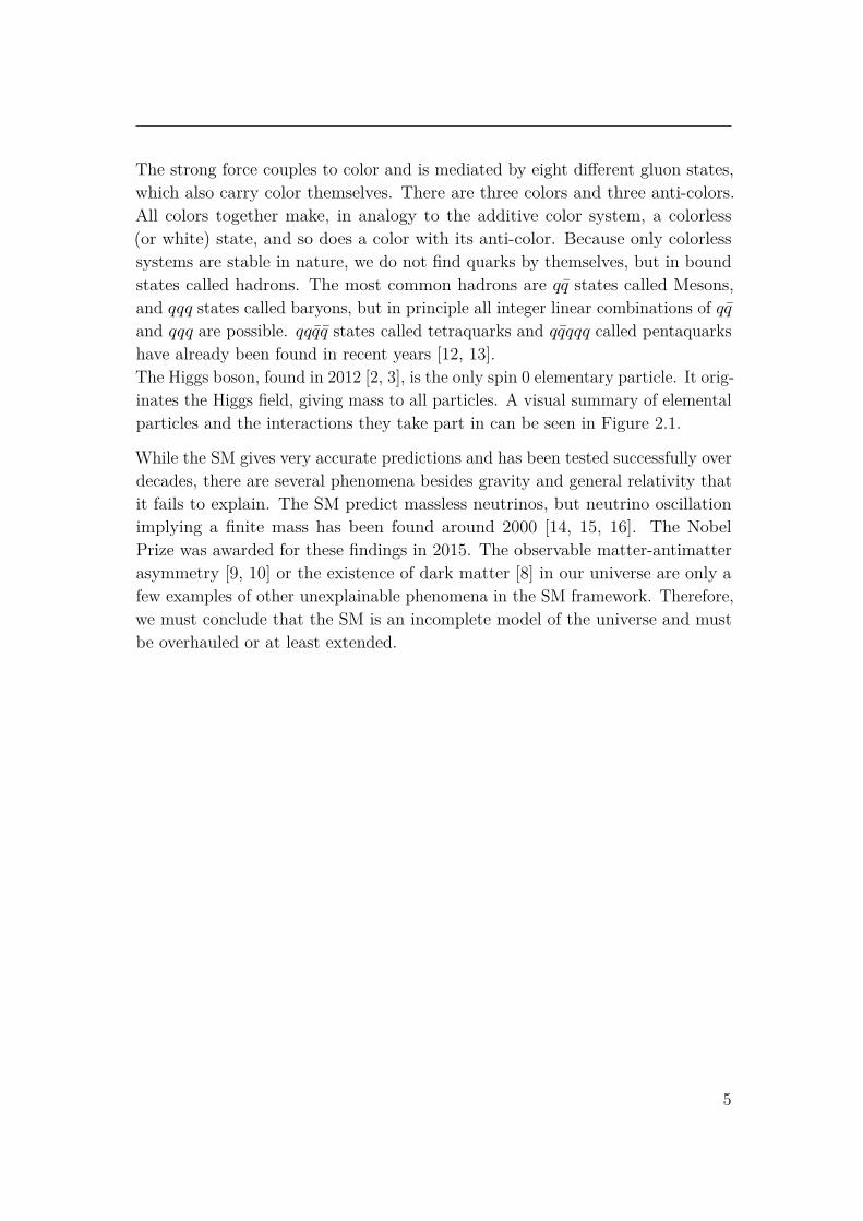
The LLT solution was rejected because it introduces large inefficiencies in hadronicbeauty and charm channels when scaled up to the operational luminosity. Figure4.1 shows the L0 yield of the B meson decays introduced in Chapter 2.1 as functionof luminosity when assuming a constant output event rate. The LLT solutionwould yield similar efficiencies. The selections performed in L0 and the LLT arenot discriminative enough to utilize the increased luminosity. After the feasibilityof the software solution was reviewed extensively [55], the LHCb collaborationdecided to implement this solution [11]. The full software trigger has the additionaladvantage that it is much more versatile and can adapt to change in conditionsfaster and easier than a hardware trigger could. The LLT could be implementedin software as a backup solution.
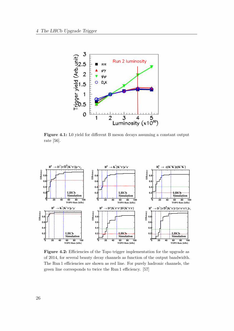
Efficiency gains due to hardware trigger removal can be showcased with Figure
24

4.1 Why upgrade to a full software trigger?
4.2. It shows efficiencies for a selection of important channels selected by themost important beauty trigger, the topological trigger, or Topo for short. TheTopo and the decay channels presented in the plots will be outlined in detail inChapter 8. The red lines correspond to efficiencies in the Run 1 implementation ofthe Topo trigger. The blue lines correspond to different output rate scenarios forthe Topo. Note that these efficiencies are not directly comparable to efficienciespresented in Chapter 8, because the former are calculated with respect to offlineselections for analyses. The gains in efficiency at the 20 and 50 Hz rate scenarioscan mainly be attributed to the removal of L0 selections. While already significantin leptonic channels, the efficiency increase in purely hadronic channels is evenmore remarkable. This is because hadronic channels are mainly selected by theL0 hadron trigger selection, which is the least efficient L0 trigger. A green linerepresenting twice the Run 1 efficiency is integrated into the plots for bettercomparison. These plots show that it is of major importance to be able to run asoftware trigger without the LLT in production. Note how the 𝐵0 → 𝐾∗𝜇+𝜇−
channel does not gain significantly with respect to Run 1, because the di-muonsignature is mainly triggered by the already highly efficient L0 muon trigger.
However, removing L0/LLT implies that the HLT system not only needs to copewith a higher event occupancy, but also with a factor 30 higher input rate andthe resulting output bandwidth. This Chapter introduces the trigger system indetail, its workflow and the challenges that LHCb meets with the removal of thehardware trigger.
25
4 The LHCb Upgrade Trigger
Figure 4.1: L0 yield for different B meson decays assuming a constant outputrate [56].
Figure 4.2: Efficiencies of the Topo trigger implementation for the upgrade asof 2014, for several beauty decay channels as function of the output bandwidth.The Run 1 efficiencies are shown as red line. For purely hadronic channels, thegreen line corresponds to twice the Run 1 efficiency. [57]
26

4.2 Upgrade trigger workflow
4.2 Upgrade trigger workflow
The planned upgrade trigger workflow can be seen in Figure 4.3. Before a triggercan run, the detector is read out and the raw event is assembled from the differentsubdetectors. HLT1 takes the raw event in small batches and processes in realtime. It sends a first loose selection based on a partially reconstructed event to adisk buffer storage. HLT2 asynchronously reads from this storage, reconstructsthe complete event and finally decides about the permanent persistence of a givenevent.
30MHzInelasticEventRate
1MHzHLT1
PartialEventReconstruction
2-10GB/sHLT2
FullEventReconstruction
1MHz
DiskBufferAlignment&Calibration
DiskStorage
dd
Figure 4.3: Upgrade trigger data flow. HLT1 has to work synchronously withthe LHC, while a disk buffer enables an asynchronously running HLT2 [58].
4.2.1 The first High Level Trigger: HLT1
The goal of HLT1 is the first educated event selection based on information from apartially reconstructed event in real time. The selection is tuned to aim for a factorthirty rate reduction, from 30 MHz incoming event rate to 1 MHz output[11].
Bunch crossings at the LHC have a highly varying complexity. This variancecomes from the fluctuating number of interactions per crossing and the high rangeof possible energies with which the partons collide. Events that have a largemultiplicity and a high occupancy in the LHCb detector typically yield lowerreconstruction efficiencies and worse signal purities. A global event cut (GEC) istherefore employed as the first step in the trigger. It is designed discard busiest10 % of all events. The sum of Upstream and SciFi multiplicities is found to be agood indicator for event complexity [11].
The HLT1 reconstruction starts by reconstructing tracks with hit informationfrom the VELO. The VELO is far away from the magnetic field, so only straight
27

4 The LHCb Upgrade Trigger
lines need to be fitted. The track candidates help to reduce the multiplicity inlater tracking stages. Based on these candidates and some information of thecurrent beam line position primary vertices are reconstructed by clustering tracksthat have been extrapolated to the beam line. The next HLT1 reconstruction stepmatches hits in the upstream tracker to a velo track extrapolation through thefirst part of the detector. A slightly curved line is fit to the hits in the UT and thefirst momentum estimate is extracted from that curvature. Because of the smallmagnitude of the magnetic field before and in the UT, the momentum estimate hasrelative uncertainties of about 15 %. Taking into account the magnetic field modeland the first momentum estimate, upstream tracks are further extrapolated intothe SciFi region, where the track candidates are matched to SciFi hits. This pushesthe momentum estimate to a relative uncertainty of about 0.5 %. A Kalman filteris applied to fit a velo track candidate, taking into account a momentum estimatefrom the other tracking stations. This decreases the uncertainty of velo trackparameters. A full Kalman filter application is too expensive for HLT1. Thesesteps conclude the HLT1 upfront reconstruction that serves as input to almostevery selection criterion applied in HLT1. An outline can be seen in Figure 4.4.
input stream
Velo tracking
Primary Vertex reconstruction Upstream tracking
Forward tracking
track fit
Selection criteria
keep event
+
discard event
-
Figure 4.4: A simplified scheme of the standard HLT1 data flow.
Selection criteria in the upgrade HLT1 are very similar to the ones employedin previous data taking periods. We realize the application of these criteria in
28

4.2 Upgrade trigger workflow
so-called trigger or selection lines. A line defines the required reconstructionsteps and requirements on certain signatures in the event topology to form afinal decision. Bandwidth reduction by selections always happens per-event inthe first trigger stage. That means that, whenever any selection considers asignature interesting, the full event information will be temporarily persisted intothe intermediate disk buffer.
Several lines require thresholds on simple properties of single tracks, others com-bine tracks to vertices and select based on these. The most prominent single trackline is tuned empirically to select tracks that are likely to originate from a bottomor charm decay and it involves requirements on transverse momentum, track fitquality and a minimum displacement from reconstructed primary vertices. A moresophisticated HLT1 selection involves additional reconstruction, specifically thecombination of two tracks into a decay vertex candidate and a subsequent vertexfit. This line can base its decision on not only track, but also vertex propertieslike the vertex quality as result of the fit and the vertex displacement from thebeam line. It provides an even more discriminative selection of beauty and charmdecays.LHCb’s physics program is not only interested in displaced signatures however.By requiring matching hits in muon chambers, we can select muonic trajectoriesin HLT1 very purely even if they show no PV displacement. This opens uppossibilities like searches for dark photons [59] and also contributes significantly tothe efficiency of most selections involving any muonic final state, like 𝐵0
𝑠 → 𝜇+𝜇−.
4.2.2 The disk buffer, alignment and calibration
After events pass the first HLT stage with a rate of about 1 MHz, they reach anintermediate persistence step within the disk buffer. The information gatheredand processed in HLT1 and stored in the disk buffer is used to perform a real timealignment and calibration of the detector. Already in Run 2 LHCb has operated areal time alignment and calibration system to enable offline-quality reconstructionin the trigger [60]. Examples of real time alignment are the adjustment of the beamline position for a primary vertexing algorithm or the recalibration of the RICHmirror system to maintain high reconstruction performance for the Cherenkovcones.
29

4 The LHCb Upgrade Trigger
Most importantly, the disk buffer allows an effective relaxation of the real timeprocessing requirement to a, to some extent, asynchronous operation of the secondHLT stage. As we can store HLT1 reconstructed data for up to two weeks, HLT2can be operated much more flexibly and efficiently based on current demands.To understand why the existence of a disk buffer can lead to increased efficiency,we must keep in mind that the LHC is not continuously running over the courseof a Run. One reason is the operational cycle of the LHC [61]. It takes at leasttwo hours to go from initial hydrogen ionization to stable beam conditions andproton beams are held in the LHC for a maximum of about 12 hours. Practicalproblems result in a higher ramp up and a lower stable beam time, resulting ina stable beam time of less than 50% on average in Run 2. Moreover, there aremachine development (MD) periods and technical stops (TS), in which the LHCalso does not run. A HLT2 running synchronously would idle whenever there isno stable beam. With the disk buffer however, the work can be distributed overtime. Figure 4.5 shows the disk buffer usage in 2016. One can see how during theshaded periods, the disk buffer got emptier as the data was processed by HLT2.In conclusion, HLT2 could utilize processing time corresponding to roughly twicethe time in which stable beam conditions were present in the LHC.
Week in 201615 20 25 30 35 40 45
Dis
k us
age
[%]
0
20
40
60
80
100
LHCb trigger
MD
TS
Figure 4.5: LHCb disk buffer usage in % in 2016. The shaded areas marktechnical stops (TS) and machine development (MD) [62].
30

4.2 Upgrade trigger workflow
4.2.3 The second HLT stage
As previously mentioned, HLT2 runs asynchronously to the LHC. It takes eventinput from the disk buffer and aims to perform offline-quality reconstruction andselections to bring incoming event rate of 1 MHz down to a bandwidth of 10 GB/s.Offline quality reconstruction refers to the most precise calculations, takinginto account all calibrations and alignment, even though that might cost morecomputing resources than simplified calculations in HLT1. HLT2 employs similarreconstruction steps as HLT1 and more. Aside from a high precision trajectoryreconstruction, the PID system involving the RICH and both calorimeters helpsto form particle hypotheses and neutral particle candidates.
Like in HLT1, the output bandwidth in HLT2 is controlled by a set of trigger lines.However, while HLT1 can use O(10) lines to perform the required bandwidth andrate reduction, HLT2 aims to distill the residing data down by another order ofmagnitude. This can hardly be achieved by the type of inclusive requirementsthat HLT1 employs. The average type of HLT2 line therefore specializes to selectonly a very specific decay structure efficiently, involving requirements on track andvertex topologies as well as PID variables. Most trigger lines perform secondaryand tertiary vertexing to try to reconstruct the entire decay chain they want toselect, as outlined in 3.3. The main disadvantage of exclusive selections is the lackof generalization. To satisfy research interests of all LHCb physicists, upgradeHLT2 needs to account for a total of O(1000) trigger lines that need to make adecision in every event. A union of all trigger line results will then decide overthe persistence of a given event. This concludes the high level description of theLHCb trigger system.
4.2.4 Building blocks for trigger software
The framework for LHCb trigger applications defines principles for the workflowthat the HLT farm uses for online event processing. It is called Gaudi. Asbase framework, it implements many generic components, the most importantof which will be outlined here. To be able to assemble many different triggerselections with preceding reconstruction in a modular fashion, Gaudi implementsthe basic building block for processing event data, the algorithm. A Gaudialgorithm is essentially a configurable function with event data input. Everypiece of reconstruction or selection software is built upon this base. Algorithmsin Gaudi interact with a data store, the Transient Event Store (TES), for their
31
4 The LHCb Upgrade Trigger
inputs and outputs. This store has the lifetime of one event. All data that isexchanged between algorithms during the event reconstruction resides in the TES.This way, several algorithms can run on the output of another. Gaudi also definesServices that handle operations which are independent of events, like algorithmscheduling, detector alignment, process configuration or provision of metadatalike detector conditions.
Configurability and the build model
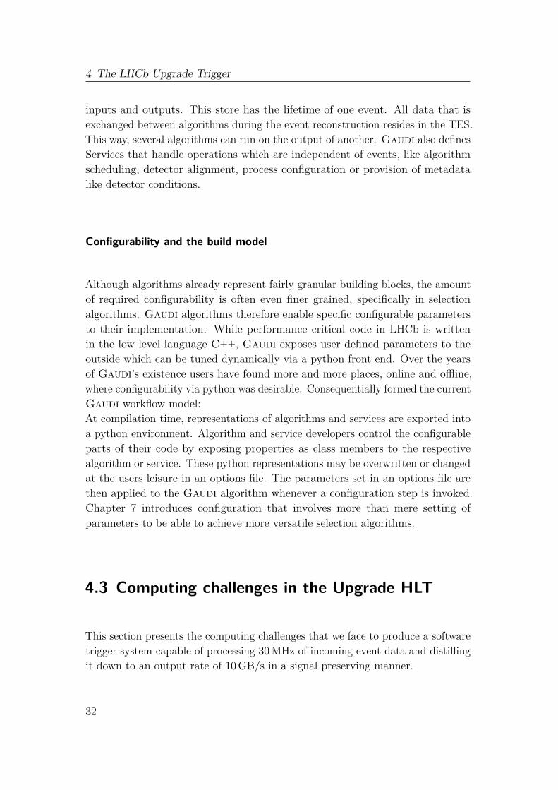
Although algorithms already represent fairly granular building blocks, the amountof required configurability is often even finer grained, specifically in selectionalgorithms. Gaudi algorithms therefore enable specific configurable parametersto their implementation. While performance critical code in LHCb is writtenin the low level language C++, Gaudi exposes user defined parameters to theoutside which can be tuned dynamically via a python front end. Over the yearsof Gaudi’s existence users have found more and more places, online and offline,where configurability via python was desirable. Consequentially formed the currentGaudi workflow model:At compilation time, representations of algorithms and services are exported intoa python environment. Algorithm and service developers control the configurableparts of their code by exposing properties as class members to the respectivealgorithm or service. These python representations may be overwritten or changedat the users leisure in an options file. The parameters set in an options file arethen applied to the Gaudi algorithm whenever a configuration step is invoked.Chapter 7 introduces configuration that involves more than mere setting ofparameters to be able to achieve more versatile selection algorithms.
4.3 Computing challenges in the Upgrade HLT
This section presents the computing challenges that we face to produce a softwaretrigger system capable of processing 30 MHz of incoming event data and distillingit down to an output rate of 10 GB/s in a signal preserving manner.
32
4.3 Computing challenges in the Upgrade HLT
4.3.1 Bandwidth requirements
Tuning the upgrade trigger towards the desired output bandwidth efficientlypresents a major challenge. The previously introduced concept of exclusiveselections alone does not satisfy the requirements. Up to now, the concepts of rateand bandwidth have been used quite interchangeably. Rightfully so, assuming aconstant event size and per-event trigger decisions. However, HLT2 employs amore fine-grained decision technique to help with bandwidth reduction, which isthe ultimately relevant merit. This kind of selective persistence already existedin Run 2 but will gain much more relevance in the upgrade. The L0 removal isestimated to cause a factor of two effective signal yield. Together with the fivefoldincrease in instantaneous luminosity this combines to an effective tenfold signalyield per unit time [63]. A factor three increase in event size with respect to Run 2is estimated based on the average number of interactions per event and the ratioof event size in a Run 2 signal event with respect to the average event size.
Selective persistence
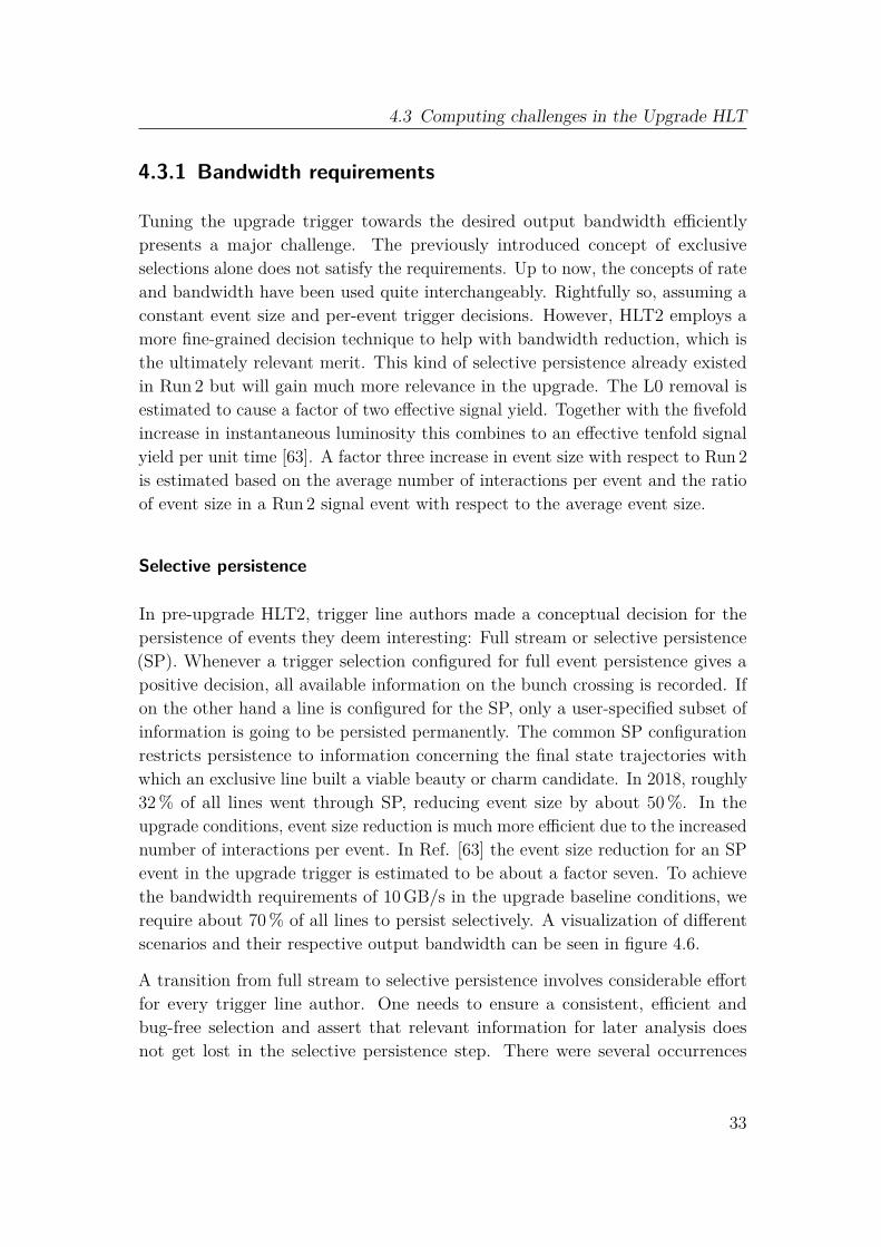
In pre-upgrade HLT2, trigger line authors made a conceptual decision for thepersistence of events they deem interesting: Full stream or selective persistence(SP). Whenever a trigger selection configured for full event persistence gives apositive decision, all available information on the bunch crossing is recorded. Ifon the other hand a line is configured for the SP, only a user-specified subset ofinformation is going to be persisted permanently. The common SP configurationrestricts persistence to information concerning the final state trajectories withwhich an exclusive line built a viable beauty or charm candidate. In 2018, roughly32 % of all lines went through SP, reducing event size by about 50 %. In theupgrade conditions, event size reduction is much more efficient due to the increasednumber of interactions per event. In Ref. [63] the event size reduction for an SPevent in the upgrade trigger is estimated to be about a factor seven. To achievethe bandwidth requirements of 10 GB/s in the upgrade baseline conditions, werequire about 70 % of all lines to persist selectively. A visualization of differentscenarios and their respective output bandwidth can be seen in figure 4.6.
A transition from full stream to selective persistence involves considerable effortfor every trigger line author. One needs to ensure a consistent, efficient andbug-free selection and assert that relevant information for later analysis doesnot get lost in the selective persistence step. There were several occurrences
33
4 The LHCb Upgrade Trigger
Figure 4.6: HLT2 output bandwidth in upgrade conditions depending on therelative fraction of the physics program using selective persistence [63]
in previous runs where data analysts benefited from information that was notdirectly related to the signal candidate. As correct reconstruction becomes moreimportant, the need for error-free software is more important than ever. A bugin the momentum-correction due to bremsstrahlung made several electron dataunusable in 2016. This would have been correctable in full stream.
Chapter 8 describes possible bandwidth optimizations including selective persis-tence for the topological B-trigger, a prominent and widely used inclusive triggerline that takes up the biggest amount of the total bandwidth.
4.3.2 Throughput requirements
Until the end of Run 2 the software HLT successfully processed an event rate of1 MHz as determined by the output rate of L0. As L0 is removed for Run 3, wewill observe a thirty-fold increase in incoming event rate into HLT1. The fivefoldincrease in instantaneous luminosity further increases computational complexity atleast linearly. We therefore require an increase in processing power by two ordersof magnitude with respect to the Run 2 HLT computing farm. The technicaldesign report for the upgrade trigger [11] laid out a detailed plan in 2014 on howto meet the requirements. More efficient reconstruction algorithms to be used inupgrade HLT1 had already been developed. A total cost estimate of 2.8 MCHF for
34

4.3 Computing challenges in the Upgrade HLT
the HLT processing farm was calculated under the assumption of a computationalpower per price growth of 1.37 per year over ten years, as seen in Figure 4.7.
Figure 4.7: Expected CPU computational power growth per time [11].
To general disappointment, the annual growth in performance per price was vastlyoverestimated. An updated annual growth rate of 1.1 has been calculated in 2017in [64].
All considerations taken together, the HLT1 stage was a factor six too slow tobe operating in 2021 with a budget of 2.8 MCHF. The HLT2 stage was notthoroughly tested in these calculations, but it was assumed to be factors awayfrom its goal.
The task is thus to achieve a factor six in computational efficiency on the givenresources via more efficient reconstruction implementations and a low-overheadframework.The low overhead framework gets much more important when we consider the taskthat HLT2 has to achieve. In Run 2, there were about 500 HLT2 lines acting oneach event at a rate of about 100 kHz. The upgrade HLT2 on the other hand willhave to manage about O(1000) trigger lines at 1 MHz input rate. The increasednumber of lines is a result of the higher degree of required exclusivity to fit intothe bandwidth limit. Another contributing factor is the broader physics programthat LHCb physicists envision for the higher data rate, making LHCb almost ageneral purpose detector. Running O(1000) lines at ten times the input rate and
35

4 The LHCb Upgrade Trigger
higher luminosity is a challenging task in which computational efficiency of theframework plays a crucial role.
36

5 Principles for High PerformanceComputing in the Trigger
There are many methods to decrease runtime of an algorithm, several of which arespecific to the algorithm itself. This chapter will first describe some general andhigher level principles for code optimization in the dominant CPU architectureof the last decades, the x86 CPU. Specifically, four phenomena will be lookedat in greater detail: Cache efficiency, predictability, dynamic memory allocationand vectorization. The last section of this chapter discusses the transition of thetrigger software to multi-threading to set context for the following chapter.
Before diving into the details, I would like to mention the most important codeoptimization technique very explicitly: Identify and restrict yourself to necessarywork. All other code optimization techniques only make sense as soon as the logicof an algorithm is minimal to achieve the task that it is designed to do.
5.1 Caching and predictability in CPUs
The first two phenomena are described together because they are often correlatedwhen one successfully optimizes an algorithm. To discuss caching, a model of CPUdata storages is shown in Figure 5.1. L1 and L2 caches reside at the core itself,while L3 is shared between multiple ones. Memory and Disk is shared over allCPUs in the machine. While the caches have a much smaller capacity than mainmemory, they are also much faster to access. When a CPU operation requiresdata in form of a memory address, the CPU loads this data from disk or memorythrough the caches into the registers the operation works on. Data is loaded infixed size chunks to populate the caches. The next time a CPU operation needsdata, it may find these data in one of the caches. The closer the memory addressis to the one required during the first load, the more likely is a so-called cachehit, meaning required data was found in the cache. A cache hit is very beneficial
37

5 Principles for High Performance Computing in the Trigger
for runtime, because the cache access times are much smaller than a load frommemory and the application can continue processing much faster.
CPU Registers
L1 Cache
L2 Cache
L3 Cache
Memory
Disk
kB
MB
100 MB
GB
TB
~ 1 ns
~ 3 ns
~ 10 ns
~ 60 ns
O(ms)
SIZE SPEED
bytes < ns
Figure 5.1: Data storage in a modern CPU architecture, ordered by physicaldistance to the compute units.
The modern CPU tries to prefetch data as much as possible. Whenever it cansee that data is going to be required in the near future, it can prepare the databeforehand to ensure a continuous utilization of compute units. However, theCPU goes even further with branch prediction. Applications often branch basedon runtime behavior. Every if statement is an example for that. The branches ofan if statement may require different data to be loaded. A CPU tries to predictthe outcome of the if statement based on historical data and prefetches the datacorresponding to the more likely branch. Applications with many branches cangreatly profit from correct branch prediction, as data dependencies are effectivelyreduced and the compute unit spends much less time waiting for data. However,efficient prefetching can only go right if an algorithm is either not branchingor if branches have very predictable outcome. To summarize, algorithms witha very linear memory access pattern have both high cache hit efficiency and ahigh predictability. They can use prefetching to utilize the available computepower well. Random accesses on the other hand kill CPU performance. Whenthe predictor fails to predict the right path, the CPU has to invoke another loadand the computation has to stall for a long while, especially when the load has togo to memory. In Chapter 7 a data model is introduced that keeps all necessaryinformation for computation close together in memory to increase cache efficiency.We also remove runtime branching wherever possible to reduce reliance on thebranch predictor.
38

5.2 Dynamic memory allocation
5.2 Dynamic memory allocation
Memory allocation in general refers to the reserve of a block of space in memoryto store some data on. There are two types of memory in a CPU, stack andheap memory. The Stack is a Last-In-First-Out (LIFO) structure on which datais simply stacked. Only data on top of the stack can be removed. The size forallocation and deallocation on the stack is defined at compile time. It is thereforereferred to as static memory allocation. If one needs a runtime specified amountof memory, one can resort to the heap memory and dynamic allocation. Theheap is randomly accessible and as such is much more versatile, but also costlyto operate on. It needs to keep track of allocated and free space and a requestfor a contiguous memory with certain size must search for such a block explicitly.During the course of execution, the heap may become fragmented. This is oftena reason for low cache efficiency and longer searches for free blocks. The CPUhas means to reduce fragmentation, but these also cost CPU cycles. Repeateddynamic allocation has been and still is a major slowdown in many algorithms inLHCb. Chapters 8 and 6 present algorithm designs that have minimal dynamicmemory allocation. If they need it, they will resort to allocation of big chunks atonce as opposed to many small ones.
5.3 Vectorization
Modern CPUs have a vast amount of instructions for loading transforming andstoring data. Vectorization refers to the usage of a specific kind of instructions:vector instructions. These instructions work on a whole collection (or vector) offloating point or integer data at once. For most scalar instructions like the addoperation, there is a vector instruction to perform the same logic on multipledata at once. The effect of a vector operation can be seen in Figure 5.2. Notethat a vector instruction has the same latency as a scalar operation, so one cantheoretically achieve a speed up by a factor equal to the width of the vectorsoperated on. In practice, the application needs to be parallelized to the degree thatusing vector operations make sense. Data to be operated on needs to be contiguousin memory. Structures might require reorganization to get the data in questioninto the right layout to use vectorization, which often costs more time thanvectorization saves. It is thus only efficient to use if multiple instructions can be
39

5 Principles for High Performance Computing in the Trigger
performed on the contiguous data, because reordering can invoke significant cost.Chapter 7 will introduce a data structure that can use vectorization effectively.
Figure 5.2: Scalar vs. vectorized CPU operation [65]. All entries in thecollections on the right need to be consecutive in memory.
5.4 Multi-core utilization with multi-threading
The single core performance of CPUs has risen exponentially, by about a factortwo every two years for over 40 years, until around 2005. This exponential growthstopped at frequencies around O(1 GHz), beyond which heat dissipation is toomuch to be cooled by air or water coolers. The key to continual performancegrowth was then found in parallelization. The first CPU with a second corewas released around the mid 2000s. That trend of increasing parallelizationhas continued to this day. Figure 5.3 summarizes the key indicators for CPUperformance in a 42-year span until 2017. AMD has released its first commercial64 core CPU in 2019. Additionally, a technique called hyper-threading came up in2002, which enabled further parallelization by assigning two processing threads toone CPU core. Two threads share the physical core, but can interleave each otherwhenever tasks on the other thread temporarily uses only parts of the resources.This typically yields a 30 % to 40 % performance boost.
The LHCb trigger application is a great candidate for parallelization as we assumeindependence between consecutive events. Independent work is an essentialprerequisite for efficient parallel execution. In Run 1 and Run 2 the triggerapplication launched multiple independent processes, each processing portions ofthe full incoming data to make use of the available computing cores. This involvesa large memory footprint as every process has to execute the entire application andno process can share memory with any other. Another disadvantage is inefficient
40

5.4 Multi-core utilization with multi-threading
Figure 5.3: 42 years trend of computational power in CPUs [66]
handling of CPU blocking operations like IO [67]. Large efforts have been putinto the development of a Gaudi application that allows multi-threading [68].This results in a cheaper thread spawn, a higher cache efficiency and a smallermemory footprint due to shared memory.
When developing a multi-threading application, one must handle the state ofthe application carefully when it can be mutated by every thread. Becauseexecution order of threads is not deterministic, incautious handling of shared statecauses race conditions that result in hardly reproducible problems. Pre-upgradealgorithms in the Gaudi application used shared state in their class instances forprocessing. In a multi-threaded application this does not allow for one algorithminstance to run on multiple events at once. As creation of new instances for everyevent cost time and memory, Gaudi transitions to an algorithm model where oneinstance allows processing over multiple events at the same time. This algorithmmodel is called ”Gaudi::Functional”.
41

5 Principles for High Performance Computing in the Trigger
Gaudi::Functional
As every algorithm may contain (configurable) state, access in a multi-threadingenvironment should only happen without mutation of said state. To enforce thiscrucial requirement as rigorously as possible for developers of reconstruction and se-lection algorithms, a constrained algorithm base implementation exists in upgradeGaudi: Gaudi::Functional. Inspired by functional languages, Gaudi::Functionalmimics the invocation of a pure function. Pure functions are defined by twoproperties:
1. Given the same inputs, it always yields the same output.2. An invocation of a pure function may never mutate state beyond its own
scope, it is said to have no side-effects.
Gaudi::Functional enforces both requirements as much as the C++ languageallows. Moreover, a functional algorithm can be read much more intuitively. Inputand output data are now part of the call signature. Inputs and outputs to legacyalgorithms may only be found within the function body.
Gaudi::Functional implements many possible input and output structures andnames them accordingly for increased readability. Figure 5.4 displays the mostcommonly used categories:
• The Consumer receives data and returns void.• The Producer generates data without inputs.• The Transformer receives and produces data.• The Merger takes a runtime-specified amount of same-typed inputs.• The Splitter generates a runtime-specified amount of same-typed outputs.
Transformer MergerProducerConsumer Splitter
Figure 5.4: Functional algorithm types in Gaudi.
The next chapter introduces a fast scheduling algorithm that multi-threads andmakes use of the features introduced with Gaudi::Functional.
42

6 A Scheduling Algorithm for the UpgradeTrigger Regime
The most significant recent change in the Gaudi framework has been the uti-lization of multi-threading as opposed to multi-processing. This change requiredthe redesign of many low level components to meet requirement of thread-safety.In the heart of the framework environment sits the algorithm scheduler definingthe logic for event processing. This scheduler must decide when to run whichtasks to achieve the result. A multi-threading application requires the schedulerto dispatch tasks to different threads such that efficient parallelization over CPUcores is possible. The first implementation of such an algorithm was defined inRef. [69]. This chapter starts by defining some concepts and nomenclature. Theexisting scheduler will then be outlined shortly. Afterwards, a new and vastlydifferent implementation to meet the LHCb Upgrade requirements better will bepresented in greater detail. Most general ideas for the new algorithm were workedout in a team of 4 people. The lower level ideas, details, and the implementationwere provided by me. It has been published in Ref. [70].
6.1 Control and data flow
Two terms used excessively within this and the next chapter are control flowand data flow. Data flow refers to the path data takes through a processingenvironment. It describes how algorithms depend on each other via the means ofinput and output relationship between them. An algorithm is data dependent onanother when its input is produced from the other. It implies that one algorithmhas to run before the other.
Control flow refers to the mechanism of controlling in which direction an applicationgoes. A basic form of control flow is a branch, for instance implemented via an ifstatement. This statement defines that under some condition the algorithm takeseither one of two paths. An equivalent, but more implicit control flow is used
43

6 A Scheduling Algorithm for the Upgrade Trigger Regime
often throughout this chapter: Short circuiting. A boolean operation can oftenbe evaluated without all operands included in the process. Consider a binaryboolean conjunction: 𝐴&𝐵. If 𝐴 turns out to yield false, then the output of Bdoes not matter for the result, it is false either way. The equivalent happens for aboolean disjunction 𝐴|𝐵 when 𝐴 yields true. Short-circuiting (or lazy) booleanoperations evaluate as soon as possible without requesting unnecessary data. If 𝐴and 𝐵 both require processing to yield an output, the processing for 𝐵 would nothappen.
6.2 The baseline: A multi-threaded event schedulerfor Gaudi
Traditionally, sequential Gaudi implemented very basic control flow. Wheneverone algorithm yields a negative control flow decision, the sequence would simplyterminate. The development of a multi-threaded Gaudi involved the creationof a new event scheduler [69]. The so-called Avalanche scheduler implementstask-based parallelism over and within events. Via inspection of data and controlflow dependency graphs of a given task collection the scheduler can maximize intra-event occupancy, thus minimize the need for inter-event concurrency. Maximizedintra-event concurrency proved to maximize peak throughput of the pre-upgradeLHCb reconstruction.
The Avalanche scheduler ranks algorithms by their importance in event processinggraph given data and control flow precedence. At any given decision step, allavailable ready-to-run algorithms are scheduled in order of descending importance.The measure of importance is motivated by the critical path (CP) of the precedencegraph, that can be calculated using the critical path method [71].The calculation of the CP involves knowledge of the runtime of algorithms in thegraph. Unfortunately, bunch crossings at the LHC vary greatly in occupancy andtopology. As reconstruction algorithms depend on these characteristics, a upfrontcalculation of algorithm runtime is nearly impossible. The Avalanche schedulertherefore assumes a uniform time distribution across all algorithms. Under thatassumption, the critical path is automatically also the longest. The only relevantimportance of a given algorithm becomes the eccentricity in the precedence graph.Eccentricity of a vertex in a graph is defined as the maximum distance to anyother vertex. Note that in this case it is defined with the precedence direction.
44

6.2 The baseline: A multi-threaded event scheduler for Gaudi
Only paths along the same direction as the arrows are considered. Rankingaccording to eccentricity has been shown to yield the best CPU occupancy andtherefore throughput results in pre-upgrade LHCb reconstruction. A visualizationof the reconstruction precedence graph with encoded node eccentricity can beseen in Figure 6.1. The more red an algorithm is colored, the higher the rankin the scheduling logic. The implementation of this scheduler in Gaudi yieldeda 34 % increase in intra-event throughput on pre-upgrade LHCb reconstructionwith respect to previous, reactive scheduling techniques [72].
Figure 6.1: Pre-upgrade LHCb reconstruction in a precedence graph. Moreintense colors correspond to greater eccentricity [69].
While this scheduler is suitable for performance regimes present in Run 1 andRun 2 LHCb, it is no option for the upgrade HLT. The dynamic aspect of thisscheduler involves much runtime bookkeeping, like the gathering of algorithmsthat have their control and data flow dependencies met at O(100) time stepsthroughout the execution of one event. The decision-making time per processedevent, given about 250 tasks, is at least 2.5 ms. This scales roughly linearly withthe number of tasks in the event.A quick estimation on CPU time per event in upgrade conditions shows that wehave little time to spare for extensive scheduler logic: Assuming roughly 1000
45

6 A Scheduling Algorithm for the Upgrade Trigger Regime
CPU nodes in the HLT processing farm, HLT1 has to run at 30 kHz per node.Let us assume a typical node in the farm to comprise about 30 physical cores.The CPU time per event calculates as follows:
𝑇event = #(nodes) ⋅ #(cores per node)𝑅tot
≈ 1000 ⋅ 3030 MHz
= 1 ms, (6.1)
where 𝑅tot is the inelastic collision rate going into the HLT. With these assumptionseach event in HLT1 has about 1 ms CPU time to be processed completely. Eventhough these assumptions may be off by several factors, the tension between 2.5 msdecision time and 1 ms processing time renders this scheduling algorithm unsuitablefor HLT1. HLT2 has about a factor of 30 more time. When extrapolating thelinear decision time of 250 tasks to several thousands per event, the infeasibilityof employing this scheduler becomes apparent in the HLT2 environment aswell.Even when assuming only 1000 tasks, the 10 ms decision time per event wouldtake about one third of the entire processing time in HLT2. In conclusion, theAvalanche scheduler is not suitable for upgrade HLT conditions.
6.3 A new scheduling application
6.3.1 From intra- to inter-event concurrency
The decision time for in-flight scheduling is a show stopper in the Upgrade HLTregime. One could reduce the decision time by bundling tasks together and thuseffectively reduce the number of decisions made per event. In fact, the mostreasonable task bundling that comes to mind is bundling full events. That meansthat scheduling logic within events has to be done statically. However, this alsomeans that task scheduling decisions become trivial as there are no dependenciesbetween events. The eccentricity of each task is 0. We call this approach inter-event concurrency as opposed to the intra-event concurrency in the avalanchescheduler. The new algorithm outlined in the rest of this chapter builds on thisidea.
6.3.2 The high level workflow
When considering only inter-event concurrency, events can be scheduled in afixed manner without computationally intensive checks or calculations during
46
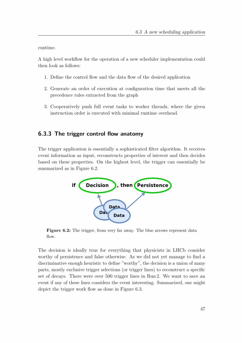
6.3 A new scheduling application
runtime.
A high level workflow for the operation of a new scheduler implementation couldthen look as follows:
1. Define the control flow and the data flow of the desired application
2. Generate an order of execution at configuration time that meets all theprecedence rules extracted from the graph
3. Cooperatively push full event tasks to worker threads, where the giveninstruction order is executed with minimal runtime overhead.
6.3.3 The trigger control flow anatomy
The trigger application is essentially a sophisticated filter algorithm. It receivesevent information as input, reconstructs properties of interest and then decidesbased on these properties. On the highest level, the trigger can essentially besummarized as in Figure 6.2.
Figure 6.2: The trigger, from very far away. The blue arrows represent dataflow.
The decision is ideally true for everything that physicists in LHCb considerworthy of persistence and false otherwise. As we did not yet manage to find adiscriminative enough heuristic to define ”worthy”, the decision is a union of manyparts, mostly exclusive trigger selections (or trigger lines) to reconstruct a specificset of decays. There were over 500 trigger lines in Run 2. We want to save anevent if any of these lines considers the event interesting. Summarized, one mightdepict the trigger work flow as done in Figure 6.3.
47

6 A Scheduling Algorithm for the Upgrade Trigger Regime
Figure 6.3: The trigger, from not quite so far away. The red arrows indicatecontrol flow dependency.
When zooming in even further, we will see that lines themselves are made upof smaller elements of boolean decision, see Figure 6.4. It becomes apparentthat a tree representation of control flow for the trigger is a suitable choice. Thetrigger decision is the first example of a higher level tree node composed of andexclusively defined by the boolean results of all trigger lines. We will call thesenodes ”Composite Nodes”. They combine decisions made by their child nodes. Thenodes filled green in Figure 6.4 correspond to ”Basic Nodes”, they represent leafsin the control flow tree. These basic nodes make decisions from reconstructed databy invoking decision-making algorithms and their data dependencies. A triggerline designed to select 𝐵0
𝑠 → 𝜇+𝜇− could define its control flow as follows: First,check if there are muons that pass some quality and displacement requirements.If there are any, see if combinations of these can build vertices with reasonableresolution. Only if both nodes yielded some candidates should the trigger line tagthe event positively.
To be able to define any control flow, composite nodes need to be able to implementseveral types of combination logic. We choose lazy-and, lazy-or, eager-and, eager-or and not. Lazy logic corresponds to short-circuiting execution outlined inSection 6.1. Eager logic schedules all children unconditionally. ”not” correspondsto boolean inversion, and requires exactly one child.
We further define optional notion of order. Composite nodes may or may not forcechildren evaluation order. A forced order of evaluation is interpreted transitively.Two composite nodes that act as children of an ordered mother imply pairwiseprecedence rules on all of their children and grandchildren.
48

6.3 A new scheduling application
Figure 6.4: The trigger, a closer view.
We can thus summarize our two types of nodes:
• A basic node governs one algorithm that makes a control flow decisionand the data dependencies for this algorithm.
• A composite node defines an execution logic and whether it forces evalu-ation order on its children, which can be either basic or composite nodesthemselves.
With the control flow design established, the next task is the representation ofdata flow.
6.3.4 Representation of data flow
Data flow in LHCb is implemented through the TES interaction. Every eventinteracts with a TES instance that is local to that event. This is crucial for practicalevent independence as we do not have to consider multi-threading synchronizationsin the data flow. Whenever an algorithm produces data, ownership over that datais transferred to the TES, and they remain there for the processing time of thatevent. TES access is done via string key lookup. Algorithms in LHCb and Gaudidefine these keys as configurable via python. Data flow is expressed as edge ofthe directed data flow graph by matching strings in output of one algorithm andinput to the other:
49

6 A Scheduling Algorithm for the Upgrade Trigger Regime
track_location = "/Event/ProducedTracks"
a = MyProducer ( OutputTracks = track_location )b = MyConsumer ( InputTracks = track_location )
MyProducer
MyConsumer
Tracks
The implementation of the pre-upgrade trigger did not allow for automation ofdata flow resolution, as TES interaction happened implicitly within the executionof every algorithm and there was no syntactical difference between properties thatdefine data flow and miscellaneous parameters. This was changed as part of thegeneral overhaul of the Gaudi framework to fit future needs.
Thus, implicit data flow is turned explicit via the use of so called ”Datahandles”.Datahandles serve multiple purposes, one of which is that they are distinguishableas special properties concerning the definition of data flow. They also provideinformation of the direction of dataflow, whether they represent output or input.It is possible to inspect algorithms for their participation in data consumptionand production.
By doing so, data dependencies can automatically be deduced for every decisionthat a trigger selection author wants to use. By matching Datahandle Inputto Output, an ordered collection of data dependencies can be built for everyalgorithm. The order is such that for every data flow edge between two algorithms,the data producer appears before the consumer in the collection.
With these ingredients at hand, the initialization and the runtime step of thescheduler implementation can be defined.
6.4 Event loop preparation - Initialization
One of the biggest differences in this scheduler implementation with respect to theAvalanche scheduler is that the order of execution is fully defined before runningover events. This is a key feature to achieve low runtime overhead.
Firstly, the control flow tree needs to be defined in the python interface. Thefollowing produces an example control flow that runs two algorithms in a short-circuiting fashion within a logical conjunction:
50

6.4 Event loop preparation - Initialization
bn1 = BasicNode ("BN1" , decision_maker1 )bn2 = BasicNode ("BN2" , decision_maker2 )
root = LAZY_AND ("root" , children=[bn1 , bn2 ] , ordered=True )
register_cf_tree ( root )
The root of the tree is registered and traversed through the children to gatherall nodes that one can reach from root. This tree is translated to C++ viathe configurable interface. From that information the algorithm creates C++
instances of all the nodes and save them with fixed positions in memory. Datadependencies in the basic nodes are filled by matching the Datahandles as discussedin the previous section. Both composite and basic nodes receive pointers to theirchildren and parents to be able to traverse the tree upwards and downwards. For allordered composite nodes, control flow precedence rules are built pairwise betweenall children, represented as control flow edges. A typical two-line configuration maylook as depicted in Figure 6.5. The red arrows represent control flow precedence,generated from the ordered mother of the basic nodes.
Line_1orderedLazyAND
DecisionunorderedEagerOR
A1 Shared A2
Line_2orderedLazyAND
B1 Shared B2
Figure 6.5: The control flow tree of a minimal two line configuration, withone shared basic node. Red arrows represent control flow edges.
Next, a valid order of execution to use at runtime is produced. All basic nodesare gathered into a set and then ordered to meet all precedence rules as definedby the composite nodes. This is done by continuously looping over the initial setand moving nodes into an ordered collection whenever all nodes that precede thisnode are already part of the ordered collection. This way control flow precedencecircles can be detected. A full loop through the set without any move operationresults in error.
51

6 A Scheduling Algorithm for the Upgrade Trigger Regime
We end up with an ordered collection of basic nodes with their data dependenciesas can be seen in Figure 6.6.
DataDataData Data
A1 A2B1 Shared B2
Order of Execution
Line_1orderedLazyAND
DecisionunorderedEagerOR
Line_2orderedLazyAND
Figure 6.6: The control flow tree with the basic nodes ordered as they willbe executed during runtime.
During runtime, the algorithm needs to maintain the state of every control flownode to ensure correct execution. Specifically, each node’s state is specified by oneinteger and one boolean. With the boolean we track the control flow decision thatevery node evaluates, either from the underlying algorithm or from the logicalcombination of other nodes. The execution counter will be further explainedin the next section. Notably, the node states are not tracked as members ofnode instances. This would require a copy of the control flow tree instance foreach event in flight. Therefore, node states are represented as part of an orderedcollection, and each node is assigned an index in the collection. It is copied intoeach event task to enable independent processing.
Although not strictly required, the same trick is performed for algorithm executionstates. At any time during the event, one can inspect algorithms for their controlflow decision and their execution state by querying an algorithm state service thatholds thread local variables to track the states. This is a feature needed for theavalanche scheduler, but thread-local access is unnecessary overhead in this case,as the scheduler can work on local instances.
52

6.5 The event loop - Runtime
Finally, a user defined number of threads is initialized. This collection is oftencalled thread pool. These threads take care of processing events.
6.5 The event loop - Runtime
6.5.1 Task packaging
The event loop is the performance crucial part of the scheduler, as everything thatwill be calculated within the loop needs to happen 30 million times per second inHLT1 and 1 million times per second in HLT2.One thread, the master thread, takes care of the actual loop over incoming events.It prepares tasks which represent the processing of one event each. Every eventtask receives a context with which it finds metadata about the event. The contextalso carries a fresh copy of the node state vector that has been prepared in theinitialization. Event tasks are then pushed into a queue.Meanwhile, idle workers within the previously initialized thread pool wait forincoming event tasks. When one arrives, any idle worker is notified, it takes thetask from the queue and immediately starts processing. If there is no free worker,the first one that finished processing directly takes up the next task. As soonas a task is done, the worker notifies the master thread about the finished event.This notification enables cooperative scheduling. Instead of filling the workerqueue indefinitely, the user can define the number of events in flight. That is themaximum number of unfinished event tasks at any given time. Unconditional fillingwould consume more memory than necessary. By just slightly overcommittingthe queue, idle workers are avoided. On the test node with 20 hyper-threads, thespeed optimum is reached with 20 workers and about 24 events in the queue.
6.5.2 Sequence execution
Within the event task, execution of the ordered sequence of basic nodes may nowbegin. To explain the algorithm, we define nomenclature:
1. A node is ”retired” as soon as its decision is evaluated. For lazy nodes, thishappens as soon as the decision of their children allows it. One negative
53

6 A Scheduling Algorithm for the Upgrade Trigger Regime
(positive) decision in a lazy-and causes retirement. For eager nodes, retiringhappens only after all children are retired themselves.
2. A node is ”requested” if there is at least one path through the tree fromthis node to the root where none of the parents in that path are retired.
The basic node sequence is looped over in the following manner:
1. Is the node requested? If not, continue with the next node
2. Every data dependency in the list assigned to the node is executed if thathas not happened before as part of another basic node. The same is donefor the decision maker algorithm. Note that it is possible that a decisionmaker is a data dependency of another node.
3. The control flow decision of the decision maker is propagated to all parentsof the node.
4. All parents update their own state depending on their composite node type.If one parent is retired, this information is propagated to its parents in turn.
Every request for state goes into the local state collection that has been copiedinto the context for the event task. So if the execution state of a node is needed,the node provides the index to look for in the state collection. The same goes foralgorithm states.
The outlined method of execution guarantees minimal work, and the introduc-tion of the scheduler into the LHCb software stack has immediately revealedunnecessary steps in the reconstruction, because data was produced that was notconsumed anywhere.
6.6 The control flow barrier - Sharing work
In the LHCb track and vertex reconstruction the very same task is sometimesperformed on different selections of tracks or vertices. These selections are notnecessarily disjoint, in which case duplicate work is done on the intersection. Wecan explore different methods of avoiding duplicated work. One method couldbe an upfront reconstruction that considers all tracks or all vertices. This maysave computation in case the intersection is bigger than the amount of data youadditionally consider when not selecting previously.
54

6.6 The control flow barrier - Sharing work
Here another method is considered: A work sharing barrier. Its job is to gatherthe union of all selections to perform the computationally intensive task on, thenexecute the task only once and afterwards scatter the data back into multipleselections accordingly. A sketch of the barrier workflow is depicted in Figure 6.7.Columns represent independent data flows merged at the gather step. In thisexample, the first data flow stopped early, as for instance control flow did notrequire further execution of the corresponding line. In order to handle these casescorrectly, the barrier requires the introduction of optional data dependencies. Thegather step needs to work regardless of how many data flows make it to that point.Only if all executions terminate early, the gathering step should not be invoked.
Figure 6.7: The gathering concept. Black arrows indicate dataflow. Thegather algorithm only considers inputs of active dataflows (second and thirdcolumn from the left).
The way this scheduler handles data dependencies and control flow precedenceallows such a barrier by introducing additional precedence rules and strategicallyplacing the gathering algorithm. A working barrier configuration is shown inFigure 6.8.
Firstly, optional data dependencies are modelled by never explicitly consideringdata dependencies of the gather algorithm. When data dependency lists are buildfor basic nodes, the gather algorithm is considered as pure producer. That wayone avoids accidentally invoking a selection algorithm that only serves an alreadyretired line, like the first column in Figure 6.7. In the example in Figure 6.8, thegray dotted arrows depict optional dependencies.
Secondly, explicit pairwise precedence rules between the inputs to the gatherer
55

6 A Scheduling Algorithm for the Upgrade Trigger Regime
and the receivers of the barrier output data need to be introduced. Otherwise,one line might be scheduled before the other, and the expensive algorithm runsbefore all inputs have been produced. These precedence rules are the reasonthis is referred to as a barrier concept. All inputs to the barrier need to havecompleted or retired beforehand before the gathering can begin. In other words,a synchronization step is introduced. The example in Figure 6.8 introduces fourprecedence rules, pairwise between Selection 1/2 and Filter 1/2.
All inputs to the gatherer need to be scheduled explicitly as decision maker of abasic node as opposed to being executed as part of a data dependency resolution.There are two reasons for that:
Firstly, explicit precedence is part of control flow which is modelled via edgesbetween tree nodes.Secondly, these inputs mostly serve the gatherer exclusively. However, inputs tothe gatherer are not considered as part of the data dependency chain due to theiroptional nature. Thus, unless explicitly requested as part of a lines control flow,these inputs would not run at all. With the proposed setup, they are explicitlyrequested as long as the parent line has not yet retired. Notably, since these dataproducers now participate in control flow as decision makers, they simply yieldan unconditionally positive decision.Lastly, our barrier should not be part of the explicit control flow, but only play arole as data dependency of any one of its successors in the data flow. If all linesretired before reaching any consumer of the output data the expensive algorithmprovides, invocation of the barrier would be unnecessary work.
Line2
Line1
Filter1Selection1....
Filter2Selection2....
SomeData ExpensiveAlgNotinControlFlow Barrier
Figure 6.8: The barrier concept built into the work flow configuration. Blackarrows represent data dependency, while the gray dotted arrows denote optionalnature. Blue blobs represent basic nodes and green blobs show data producers.
56

6.7 Scheduler performance
6.7 Scheduler performance
Performance measurements were performed for multiple scenarios to ensure suffi-cient computational efficiency even in complex scenarios.
The first test involves the execution of the HLT1 reconstruction chain. As itrepresents a linear sequence, it can be scheduled explicitly with a minimal logicscheduler implemented in Gaudi. This scheduler invokes a full event stop whenevera negative control flow decision is encountered. No throughput difference couldbe observed between both schedulers after averaging several runs, meaning thatthe logic introduced in the new implementation causes negligible overhead in thiscase. This is not a representative stress test however, as the HLT1 reconstructiononly involves linear control flow with about 15 algorithms.
For following tests, the Intel V-Tune Amplifier [73] is employed to estimate functionexecution times in multi-threaded environments without significant overhead tothe application. Fully fledged HLT environments are mocked with algorithms ofconfigurable busy execution time.
When calibrating the application to the nominal HLT1 throughput requirementof 30 kHz with 10 lines and 5 nodes per line on 40 threads, the schedulers relativeconsumed CPU time stays well under 0.5 %. Doubling the number of lines at thesame throughput level brings the contribution to execution time up to nearly 1 %.However, other framework overheads surpass the scheduling overhead.
A HLT2 like scenario is also tested to ensure scalability of the implementation.500 lines with 10 nodes each are calibrated to a throughput of about 1 kHz.The relative time contribution stays well under 2 % here. Unfortunately, otherframework overheads scaling badly with increasing number of algorithms slowdown the application much more. Further framework bottlenecks need to beinvestigated until we are ready for a 1 MHz HLT2 application.
6.8 Summary and outlook
I have presented the first production ready scheduling algorithm that meets thefeature requirements for the upgrade HLT. All in all, the undertaken tests showpromising results that runtime overhead is sufficiently small for use in the onlineHLT environment. As of this day, it is the baseline scheduler used in all CPU
57

6 A Scheduling Algorithm for the Upgrade Trigger Regime
upgrade configurations. The GPU implementation for HLT1 in Allen is currentlyadopting an implementation that has been derived from this one. It enables theoption of packaging multiple events into one task.
The only real test for the overhead of the scheduler implementation will be thefull HLT2, once it is fully implemented. Until then, there are some changes thatcan marginally speed up the scheduling time.
In the HLT many selection algorithms have a long tail of data dependenciesthat are similar for many nodes, invoking the full track reconstruction to get theparticle inputs. Even though these algorithms are not actually run multiple timesper event, there are still lots of unnecessary if-statements to go through. Onecan therefore explicitly schedule these common reconstruction steps upfront andinvoke the following optimization: Whenever a basic node dominates another,all shared data dependencies can be removed from the latter. ”A dominates B”means that execution of B implies previous execution of A.
Secondly, most of the explicit scheduling time is spent in checking whether abasic node is requested, an operation that has to go up the control flow tree.Conceptually, an invocation condition in dependence of other basic nodes could bededuced at configuration time already. This would effectively avoid tree traversalfor that particular operation.
58

7 Selections and Combinatorics in UpgradeHLT2
After having written and optimized parts of the underlying application frameworkfor the upgrade trigger in the last chapter, this chapter focusses on two specificalgorithms of HLT2 itself, where significant improvements have to be achieved inorder to get the desired runtime efficiency. After an introduction to the use casefor these algorithms in Section 7.1, the performance of status quo is discussedin Section 7.2. Section 7.3 discusses these algorithms in detail. The followingsections discuss several solutions to optimize the algorithms in question. Lastly, asummary on the current state and an overview on future work are given. Notethat the work presented in this chapter is the outcome of shared efforts betweenOlli Lupton and me. Several other people in the LHCb collaboration helpedforming the ideas.
7.1 Selection algorithms in the trigger workflow
The outlined HLT1 workflow in Figure 4.4 is conceptually similar to HLT2. Asmost trigger lines require a common set of reconstruction algorithms, control flowcan be slightly simplified by invoking an unconditional upfront reconstructionstep. Although the specifics of the reconstruction in HLT1 and HLT2 are different,both trigger stages have one thing in common. After upfront reconstruction, mostof the leftover work is done by selection algorithms, represented as the ”selectioncriteria” in Figure 4.4.
In HLT2 one mainly differentiates between two types of selecting algorithms. Thefirst type is the plain selection that takes a collection of particles and returns aselected collection. These are called ”Filters”. An example of a Filter is one thatcollects muons with a high transverse momentum from all the input particles.
Algorithms of the second type are called ”Combiners”. These algorithms combinetwo or more particles to form a candidate for a decaying particle. Although
59

7 Selections and Combinatorics in Upgrade HLT2
combiners reconstruct vertices, they will be referred to as selection rather thanreconstruction algorithms, because selection criteria with control flow impact areapplied at multiple points during the combination process.
Many Combiner and Filter instances in HLT2 apply tight requirements suchthat most invocations end up with an empty output collection, meaning that noparticle passed all selection criteria. Control flow decisions for the trigger arebased on whether at least one particle passed the algorithm. The typical workflowof a trigger line selecting 𝐵0 → 𝜋−𝐾+ can be seen in Figure 7.1. It is assumedthat charged final state particles are already reconstructed and classified via PIDinformation. To build 𝐵0 → 𝜋−𝐾+, one first needs pions and kaons. Becausethey should come from a beauty decay, one may filter based on displacement fromthe primary vertices and a high transverse momentum. This is what the Filtersare designed for.
The following workflow is comprised within the implementation of Combiners. Ifthere are pions and kaons matching the criteria, the next part of the workflowcan be invoked. The selected final state particles can be combined and selectionscan be made on these combinations. Examples would be the distance of closestapproach between both particles. If there are good combinations, a decay vertexfor the 𝐵0 candidate can be fitted. If this vertex passes some more requirements,a 𝐵0 candidate is selected for final persistence. The decision of the Combinerdepends on whether any candidate passed all previous criteria.
60

7.1 Selection algorithms in the trigger workflow
Reconstructtracks +particles
Pion selection
Kaon selection
Selectcombination
Fit vertex
Select Bcandidate
Triggerdecision
Persistcandidate
Control FlowData Flow
At least onePion
At least oneKaon
At least onecombination
Combine Kaon+ Pion
At least onecandidate
Particles
Particles
Pions
Kaons
K+pi combination
K+pi combination
B candidate
B candidate
Raw event
Figure 7.1: The reconstruction workflow in a trigger line selecting𝐵0 → 𝜋− 𝐾+. Blue arrows mark data flow and red arrows correspondto control flow.
61

7 Selections and Combinatorics in Upgrade HLT2
7.2 Runtime performance in status quo
Significant throughput improvements have to be achieved to reach the throughputgoal of 1 MHz in HLT2. Exact numbers are hard to come by, as only about300 out of an estimated O(1000) trigger lines are currently available in upgradesoftware. Current benchmarks with the existing lines show that HLT2 throughputis off by at least a factor of 2. The Combiners and Filters this chapter focuses oncontribute about 25% to the overall runtime.
The benchmark in Figure 7.2 compares this to the Run 2 HLT2 implementation onHLT1 filtered upgrade simulation. On a single core of an Intel Xeon E5-2630-v4CPU, this configuration processes events at about 2 Hz. Filters and Combinerstogether use about 23% of the total runtime, and this configuration only consistsof about 450 lines as opposed to the O(1000) lines expected for the Upgrade.
Figure 7.2: Relative execution times of the top 10 algorithms in the Run 2HLT2 on upgrade HLT1 filtered simulation. The Combiner and Filter barssum all combiner and filter instances. All other algorithms refer to parts ofthe reconstruction. Specifically, the TrackBestTrackCreator is the algorithmperforming the track fit.
62

7.3 The baseline algorithms
7.3 The baseline algorithms
The baseline Filters and Combiners in HLT2 are called ”FilterDesktop” and”CombineParticles”. Both act on collections of particles as inputs. FilterDesktopreturns a selected subset of the input particles, while CombineParticles createsnew candidates from the combination of the inputs.As these are very generic algorithms, several aspects are configurable throughthe python interface, like the decay to be reconstructed in the combiner and allselection criteria.
7.3.1 Filtering with LoKi
Being able to define generic selection criteria from a python interface to theC++ code is a non-trivial task. In the early days of LHCb, criteria would stillbe hard coded into the algorithms, with configurable parameters only. It wasthen possible to change the minimal transverse momentum threshold from theconfiguration, but not the fact that it is a minimum transverse momentum cutwithout editing C++ code. A dramatic improvement to usability came with theintroduction of the LoKi (Loops & Kinematics) framework [74], which providedthe implementation of so called LoKi-Functors. These allow the definition ofalmost arbitrary selection code via specification though a python string or directlywithin a Gaudi algorithm. With LoKi, selection code can be defined as follows,from python:kaons = reconstruct_kaons ( )MyKaonSelector = FilterDesktop (
input=kaons ,Code="(PT > 1*GeV) & (IP > 1*mm)"
)
A python interpreter will interpret the Code string at initialization time of theapplication. PT and IP are python aliases for C++ classes that are accessiblefrom python via the cppyy interface [75]. Different kinds of unary and binaryoperations on these objects are overloaded to yield composed LoKi functor types.For instance, PT > 5∗GeV constructs a class with a call operator returning a boolean,checking whether the input has a transverse momentum of more than 5 GeV.Compositions via mathematical operations like +,−,∗,/, boolean compositions &,|,~and more are supported in the LoKi framework. Functors can be transformed to
63

7 Selections and Combinatorics in Upgrade HLT2
a C++ representation of themselves that is accessed from the filter and combineralgorithms to perform the desired selection. It is thus possible to create arbitraryselection predicates without any additional compilation, sufficient for almost alluse cases in the LHCb selection framework.
7.3.2 Basics of combining
The process of combining particles to a common parent has been introduced withthe 𝐵0 → 𝜋−𝐾+ example in Section 7.1. This section will go into more technicaldetail, starting with a summary of the workflow:
1. Take m input particle collections, where m is the number of different particletypes.
2. Select the children collections with reasonable criteria for the given decay.
3. Build a n-body combination from these particles, where n is the number ofchildren of the parent to be reconstructed. This is a 𝑂(𝑘𝑛) scaling operation.
4. Select combinations with criteria to match a good candidate. These criteriado not only involve user-specified predicates based on the decay, but also apairwise overlap check. When two particles share underlying componentslike tracks, a combination can not yield a valid signal candidate, so theseare preemptively discarded.
5. Fit the combination to yield a decay vertex position and a parent momentumwith respective uncertainties.
6. Select good vertices and label them according to the decay requirement.
This workflow is performed in almost every HLT2 line in LHCb, often multipletimes per line execution. It is notable that the number of operations involved scaleexponentially with the number of children involved, so critical path efficiency iscrucial for a successful online application. Efficient evaluation of selection criteriabecomes very important as these have to be applied to every combination.
64

7.3 The baseline algorithms
7.3.3 Workflow in the baseline combiner
CombineParticles has worked as the default combiner algorithm throughout alloperational years of LHCb. It is based on the Run 2 HLT2 particle implementation:LHCb::Particle. LHCb::Particle is a structure that holds multiple properties likeparticle ID information and possibly a decay vertex or a track. As the class is notspecific to the type of particle, a charged final state particle has a nullpointer for thedecay vertex and a composite particle has a nullpointer for the track. The designof LHCb::Particle is discussed in more detail in Section 7.5.1. CombineParticlescan receive either selections or vectors of particles to be agnostic on whether aprevious selection has been applied to the collection. The algorithm is subdividedinto three stages: Child-, Combination- and Vertexing-stage.
At first, the algorithm parses a decay descriptor. This is a user specified stringthat encodes the decay to be reconstructed by the combiner. An example decaydescriptor is given here:"[B_s0 -> D_s0 pi+ pi-]CC"
It encodes several important pieces of information for the combiner: The numberof children (3), the particle id of combined particle (𝐵0
𝑠), the children particle idsand their charge configuration. The CC serves as shortcut for charge conjugation.Wrapping the decay descriptor with brackets and CC means that the chargeconjugated decay is also to be reconstructed in the same combiner invocation.CombineParticles generally allows for an arbitrary long list of decay descriptorsto be worked off at the same time. Reconstructed parent particles from all decaydescriptors will later be put into a common collection to be stored on the TES.Decay descriptor parsing and LoKi cut generation are the two main things thathappen before or during initialization, they do not contribute to runtime costs inthe event loop.Selection criteria logic for cuts on input particles works as follows: The userprovides a map of particle ID (PID) to criterion. When there is no entry for aPID that occurs in a decay descriptor, the criterion will fall back to either thecriterion of the charge conjugated PID, or if neither exist, to no selection criterionat all.
A user can give an arbitrarily long list of input particle collections to the combiner.In the child stage, input particles are merged into a single container per PID.According to the decay descriptors and the child cut dictionary, relevant particleswill be selected for consideration in the combination stage.
65

7 Selections and Combinatorics in Upgrade HLT2
The combination and vertexing stages happen within a loop over all decay de-scriptors. A n-dimensional loop over the relevant input particles given the currentdescriptor is built. It corresponds to the cartesian product of the input vec-tors. The first check on each combination is for uniqueness. It is trivial forcombinations with disjoint PIDs because particles with different PIDs are perdefinition different. However, it is important for any decay descriptor in which onePID occurs twice, like 'B+ -> pi+ pi+ pi-', where one does not want to considerboth (pi+[x], pi+[y], pi−[z]) and (pi+[y], pi+[x], pi−[z]). x,y,z represent indices intothe pion containers. The uniqueness check asserts that only combinations areconsidered in which particles with the same PID are ordered in some way. Theorder criteria comprise kinematic and pointer comparisons. The result for selectedcombinations is depicted in Figure 7.3. Note that checks for unique entries ina collection usually scale 𝑂(𝑛2) with the number of elements, while this orderrequirement can be applied with 𝑂(𝑛) scaling. Producing a complete collectionof unique combinations with the order requirement can only work correctly ifthe containers of which the combinations are made are exactly the same. This isthe reason for the merge of all inputs according to PID in the child stage. Thecombiner functionality is therefore restricted to one cut per PID, not one perinput collection.
(0,0) (0,1) (0,2) (0,3)
π+ container0 1 2 3
0 1 2 3π+ container
(1,1) (1,2) (1,3)
(2,2) (2,3)
(3,3)
π- container0 1 2 3
0 1 2 3π+ container
(1,0)
(2,0)
(3,0)
same PID different PID
(0,1)
(1,1)
(2,1)
(3,1)
(0,2)
(1,2)
(2,2)
(3,3)
(0,3)
(1,3)
(2,3)
(3,4)
(0,0)
(1,0)
(2,0) (2,1)
(3,0) (3,1) (3,2)
Figure 7.3: Loop structure for combinations of containers with either same(left) or different (right) PID in a 2D subspace. Assuming the containersare ordered according to the aforementioned kinematic criteria, green fieldsrepresents considered combinations.
Next, all combinations with an overlap are filtered out. There are multiplealgorithms that define what overlap means, but conceptually one tries to identify
66

7.3 The baseline algorithms
whether multiple particles in the combination have been made from the sametrack or with the same calorimeter clusters. Nothing stops two algorithms fromdefining two different particles from the same track by assigning two differentparticle IDs. No track or cluster information in the detector should go into thereconstruction of two disjoint particles.
The algorithm proceeds to apply the combination cut, one of previously definedselection criteria. In HLT2, trigger line authors often require a small distance ofclosest approach (DOCA) between the combined particles or that at least oneinput particle had a high transverse momentum. The application of selections onthe particle combination serves the purpose of reducing combinatorial load on thesubsequent vertex fit.
The last stage in CombineParticles is the vertexing stage. The few particlecombinations that have made it through all previous checks and selections arenow fitted into a common intersection point, or vertex. Out of a successful vertexfit comes a vertex position and a covariance and a fit 𝜒2, which is then associatedto a new particle, the parent candidate for all children in the combination. ItsPID is set to the parent PID in the decay descriptor. These candidates are thenselected again with a user specified criterion, most often based on the vertex 𝜒2,invariant mass and vertex position. Particles passing the entire selection chainare persisted into the TES for further studies.
Next to CombineParticles, there is another set of algorithms called ”NBodyDecays”.These algorithms are, unlike CombineParticles, specialized on the number ofchildren to be combined. They enable another set of user specified criteria thatwe will call sub-combination criteria in this chapter. When combining N children,cuts on the [2..N-1] combinations may also be specified to reduce the combinatorialphase space early on. A simplified three body combination loop might look asfollows:
for p0 in particle_container_0 :for p1 in particle_container_1 :
# do not even ente r the th i rd loop i f# the two body combination i s ”bad”if not two_body_cut (p0 , p1 ) :
continuefor p2 in particle_container_2 :
if three_body_cut (p0 , p1 , p2 ) :do_vertex_fit_and_cut (p0 , p1 , p2 )
67

7 Selections and Combinatorics in Upgrade HLT2
7.4 Improving upon the baseline with newselections
The first version of LoKi has been introduced as the framework for composableand configurable selections over a decade ago. The functional, multi-threadingframework is however ill-suited for the use of many LoKi features that rely heavilyon internal state. As many people want and require configurable selections, arewrite of major parts of the LoKi framework would be necessary for use in theupgrade HLT. However, benchmarks within HLT1 selections have uncovered thatLoKi selections often are the bottleneck of the application.
We therefore decided that developing a completely new selection framework ismore sensible. This framework, dubbed ThOr (Throughput Oriented) is beingdesigned with different levels of parallelism in mind. It is fully functional toease multi-threading, and its type system makes the use of vectorization withinselections easier than LoKi does.
While ThOr aims to provide similar functionality, its C++ backend is different toLoKi’s. LoKi works with cppyy’s python bindings and it resorts to type erasure onmultiple levels to be able to compose functors at runtime without any additionalcompilation. While this is a very flexible approach, it comes with a non-negligibleruntime overhead. Every composition adds more costly runtime polymorphism.
The backend of ThOr on the other hand does not try to avoid additional compila-tion. With the cling compiler [76] that has been developed after the introductionof LoKi, Just In Time (JIT) compilation is available in the LHCb software stacknatively. Rather than stacking layers of costly polymorphism, ThOrs functorscan get JIT compiled and linked at the initialization time of the HLT application.There is only one layer of type erasure that enables the use of ThOr functors inany Gaudi algorithm.
Cling is a JIT compiler currently based on Clang 5. Compared to the currentlyused compilers in LHCb software, Clang 9 and GCC 9/10, Clang 5 is fairly old anddoes not support the newest C++ standards. This fact in itself poses challengesdue to incompatibility, but that is not the only problem. Code compiled with clingoften executes many factors slower than code compiled with modern gcc or clangversions, the reason for which is currently under investigation. Moreover, changingcompiler flags to enable different levels of vectorization is highly non-trivial incling as it uses pre-compiled headers of ROOT libraries that it depends on. JIT
68

7.4 Improving upon the baseline with new selections
compilation of ThOr criteria is thus done exclusively on a scalar basis, i.e. novectorization enabled.
In summary, JIT compilation with cling is currently not efficient for high through-put scenarios, but it works fast enough for the offline use without the need torecompile the full software. For the high throughput production application, ThOremploys a second mode of compilation: The functor cache.
All functors that are defined in python during build and compile time will becompiled into a cache to be used natively in the application. The usage of thesefunctors does not need any JIT compilation.
Note that LoKi is also capable of using a functor cache, but the performancedifference is much less pronounced than with ThOr. This has two reasons: Firstly,the slowdown that Cling introduces with its JIT compilation only applies to ThOr,as LoKi does not necessarily need to compile anything. Secondly, the extensiveamount of type erasure that enables composability without compilation is stillpresent in compiled functors. Figure 7.4 summarizes the possibilities to buildconfigurable selections and their runtime qualitatively. The speed differences havenot been quantified for the two slower options as they can be avoided duringproduction. Detailed comparisons between compiled LoKi and ThOr are foundlater on in this Chapter.
faster
JIT ThOr LoKi
cachedLoKi
cached ThOr
assembledduring
intialization
pre-compiled
Figure 7.4: Functor implementations sorted by speed (single-core only, quali-tatively).
ThOr implementations of functors are already put to practice in HLT1 selectionsand yield good results there. For the first tests in HLT2, ThOr functors are
69

7 Selections and Combinatorics in Upgrade HLT2
implemented to work with LHCb::Particle.
Generally, ThOr functors are designed to be agnostic to input and output type tobe flexible on what they operate on. They only assume the existence of certainaccessors needed to compute the desired result. This approach usually referred toas duck typing. instance.momentum() or instance.pid() are basic examples. Excep-tions are sometimes made for more mature models like LHCb::Particle as APIchanges there are much more convoluted and would require changes throughoutthe entire downstream codebase. In this case, the functor input type is detectedat compile time and another code branch is executed.
Comparisons of runtime in this chapter are all single core tests, as LoKi isnot capable of multi-threading. First order Linear scaling in the number ofphysical cores is expected, as there is no inter-event dependency in any of thesealgorithms.
The baseline filtering algorithm FilterDesktop using LoKi is compared to anequivalent filtering algorithm using ThOr called PrFilter. PrFilter is a genericfiltering algorithm which can be specialized on the type of input container. Forthis comparison it is specialized on a non-owning masked collection of LHCb::Par-ticles. Benchmarks of ThOr, LoKi, combiner and filter algorithms depend onthe configuration that is tested. Therefore, performance numbers are not to beconsidered representative for the overall HLT application, although the bench-marked selections closely resemble actual existing HLT2 selections. Note that allbenchmarks are performed with the fastest configurations which are not necessarilythe default.
Table 7.1 shows two benchmarks for each filter type. These and all followingbenchmarks in this chapter are performed over 10000 simulated events thatresemble actual production data as closely as possible. These simulations arereferred to as ”minimum bias” in LHCb. Charged basic particles are filteredaccording to two different criteria. The first number corresponds to a selectionwith only one functor, ISMUON. This functor simply dereferences some pointers tocheck whether a particle has information from the muon stations. This simplecomparison is helpful to identify framework performance differences. Since many ofmore complicated functors are implemented differently, the throughput differencesin these originate not only from choosing between ThOr and LoKi, but also byfunctors themselves. The other criterion is fairly realistic preselection to many
70

7.4 Improving upon the baseline with new selections
beauty and charm trigger lines that selects high momentum displaced tracks.Specifically, this preselection selects based on momentum, transverse momentum,𝜒2(IP) and PID. The speed up in this case can not only be attributed to theincreased framework efficiency. Specifically the calculation of 𝜒2(IP) differs. TheThOr implementation is explicitly specialized and optimized for charged basicparticles while the LoKi employs a more general, but also more costly algorithmmaking up about 60% of the 171 µs.
ISMUON displaced presel.FilterDesktop 11.6 µs 171 µsPrFilter 4.6 µs 12.8 µs
Table 7.1: A benchmark comparing two selections with two different algorithms.Both Filters work without data copy, only with indices and pointers. PrFilteremploys functors implemented in the ThOr framework.
Overall, there are many places throughout LoKi functor implementations whereperformance is sacrificed for generality, convenience or not strictly necessary fea-tures. For instance, several frequently visited branches in the ISMUON calculationyield atomic increments of logging counters. In the benchmarked scenario whereone selects muons from all long tracks, counter increments happen about 10 %of the time. If not explicitly disabled, these increments drive the execution timefrom 12 µs to 45 µs.
7.4.1 Combining with ThOr
It is now established that ThOr functor implementations work well in filteralgorithms and yield significant throughput improvements, aided by the increasedefficiency of the ThOr framework itself. The next step is thus to try to apply ThOrin the other selection algorithms, the combiners. The implementation presentedhere is the first multi-threading capable combiner, implemented in the Gaudifunctional framework. Combiners make up a major portion of the HLT2 runtimeand therefore represent a crucial component for optimization.
The algorithm described here is referred to as ThOrParticleCombiner and itsdifferences to CombineParticles are mainly framework based. It is a Merger asdescribed in 5.4. It gathers over multiple particle input containers, combinesparticles from these according to a decay descriptor and then creates parent
71

7 Selections and Combinatorics in Upgrade HLT2
particles in a vector collection. ThOr functor specializations are used for selection.This combiner specializes on the number of children at compile time, similarlyto NBodyDecays. Up to the functor implementations, the children selections areimplemented in the same way as the LoKi combiners. The differences are to findin the combination loop:
1. NBodyDecays allows for N-1 combination criteria for an N-Body combina-tion, concerning the first M children, where M goes from 2 to N. A 4-Bodycombination allows for combination cuts on children (12), (123), (1234).The new algorithm allows also for combination cuts on children (13) and(14). This helps with reducing the combinatorial load even more than inNBodyDecays. Other combinations of criteria, like (23), make less senseto implement since they would have to be evaluated as often as the (123)combination due to the loop order. One could hoist the evaluation out of theloop by preemptively applying the (23) criterion to the full input collectionsand save the result in a 2-dimensional structure, but as combination cuts aregenerally expected to have a rather small efficiency, only little informationin the 2d structure would actually be used.
2. The information on whether there are multiple instances of the same PID ina decay descriptor is only available at runtime. However, the PID check isperformed in LoKi combiners for every combination. The new combiner liftsthis information out of all loops and thus reduce the branching in criticalpaths.
The overlap check during combination is done with the same tool as in theLoKi combiners. The vertexing stage also employs the same logic as LoKicombiners, which is simply a filter step. Table 7.2 shows how CombineParticles,NBodyDecays and ThorParticleCombiner compare in runtime when using acommon 𝐷+ → 𝐾+𝜋+𝜋− selection with similar, but looser selections than in theRun 2 HLT2 𝐷+ → 𝐾+𝜋+𝜋− trigger line. The combinations are made from kaonsand pions selected with the previously benchmarked displaced filtering criteria fromTable 7.1. The combination selection involves minimum transverse momentum,distance of closest approach (DOCA), invariant mass, summed children momentum,and several more displacement requirements. After the vertex fit, selection criteriaare based on vertex quality, parent flight distance and direction angle. The bigperformance gap between CombineParticles and NBodyDecays is explainable bythe fact that CombineParticles does not allow for sub-combination cuts and thushas to evaluate many more combinations than the other algorithms.
72

7.5 A new particle model
𝐷+ → 𝐾+𝜋+𝜋− execution timeCombineParticles 256 µsNBodyDecays 77.1 µsThorParticleCombiner 38.8 µs
Table 7.2: A benchmark comparing a typical 𝐷+ → 𝐾+𝜋+𝜋− combinationwith different combiners. CombineParticles and NBodyDecays use LoKi func-tors, ThorParticleCombiner uses ThOr.
Overall, the implementation logic is very similar in all combiners that havebeen introduced up to now. Many aspects of the logic are constrained by theLHCb::Particle model. In benchmarks of the algorithms it turns out that theoverlap check is a bottleneck in the baseline combiners. This is even the casein the combination of basic particles where the implementation boils down toa couple of pointer comparisons. Dynamic memory allocation appears in everyoverlap-check invocation, regardless of the particle type. As overlap checking ispart of the critical path, this contributes a lot to the algorithm runtime.
7.5 A new particle model
The performance improvements in the previous section are promising and motivateto go further. Several key design choices in the HLT2 data model seem to hinderperformance. Changes in the data layout have already been found to unlocklarge gains in HLT1 [77]. These changes mostly concern the minimization ofdynamic memory allocation, the respect of cache locality and a data layout toenable parallelism on the level of vectorization. As long as the right accessors areimplemented, ThOr functors can work on any data layout.
7.5.1 Data layouts and LHCb::Particle
When designing a model in the object-oriented paradigm, a class usually representsan object to be described.struct Point3D {
float x , y , z ;} ;
73

7 Selections and Combinatorics in Upgrade HLT2
When describing multiple points at once, one then resorts to collections over Point
instances:using N_Points = std : : array<Point3D , N>;
This data layout is referred to as Array-of-Structures (AoS). For contiguouscollections, the memory layout of such a collection of points looks as depicted inthe upper half of Figure 7.5. All features of one point are contiguous and spatiallydisplaced from features of other points.The LHCb::Particle is designed as such a structure, displayed here in a simplifiedmanner:struct Particle {
ParticleID m_pid ;Vertex∗ m_decay_vertex ;std : : vector<Child∗> m_children ;Track∗ m_track ;. . .
} ;
The second, less intuitive layout is called Structure-of-Arrays (SoA) and is shownin the bottom half of Figure 7.5. Instead of representing multiple points by acollection of Point class instances, one can transpose the layout to three collections,one for each feature of a point:struct N_Points {
std : : array<float , N> x ;std : : array<float , N> y ;std : : array<float , N> z ;
} ;
This achieves contiguous features in memory as opposed to contiguous structuresin AoS.
Multiple LHCb::Particle instances are always represented in AoS fashion, whichbrings advantages as well as disadvantages.
The biggest advantage is intuition and readability. Encapsulating and combiningproperties into structures that have meaning is a much more natural step fora human than packaging features independently. A particle means more tosomebody reading the code than a collection of x positions. Moreover, it is morenatural to represent a single particle in AoS than in SoA, which is useful for manyuse cases in LHCb, like traversing a particle’s decay chain.
74

7.5 A new particle model
x_0 y_0 z_0 ... x_N y_N z_N
Point 0 more Points Point N
AoS
x_0 ... x_N y_0 ... y_N z_0 ... z_N
SoA
all x values all y values all z values
x_1
Figure 7.5: Array of Structures (AoS) vs Structure of Arrays (SoA).
The biggest disadvantage is SIMD performance. SIMD, or Single-Instruction-Multiple-Data, is a programming paradigm where the task can be formulatedas a single sequence of instructions that has to be applied to a lot of data,element-wise:
//AoSstd : : array<Point , N> points , other_points ;array<int , N> x_sums ;for ( int i = 0 ; i < N ; ++i ) {
x_sums [ i ] = points [ i ] . x + other_points . x [ i ] ;}
//SoAN_Points points , other_points ;array<int , N> x_sums ;for ( int i = 0 ; i < N ; ++i ) {
x_sums [ i ] = points . x [ i ] + other_points . x [ i ] ;}
While these operations look very similar and accomplish the same thing, there is
75

7 Selections and Combinatorics in Upgrade HLT2
one crucial difference. The SoA loop accesses contiguous elements as it evolves.For each new i, one just adds 4 bytes to the previously used memory addresses.The AoS loop does not access memory contiguously and has to jump the size ofone Point every time to get to the next x value.
There are at least two reasons to prefer the SoA loop. Firstly, the cache hit rateis very high. The AoS loop on the other hand uses only about one third of thedata received by one cache load, and it gets worse the more members a structurehas.
Secondly, CPU vector instructions operate on contiguous memory. Because theSoA layout naturally ensures the dense memory structure in each feature, that loopcan be transformed to use vector instructions quite natively. As these instructionsare almost as fast as scalar instructions, speed-ups of up to 8-fold can be achievedwith modern CPU vectorization. Real life use cases naturally bring their caveats,but they can often be outweighed using vectorization in a sufficiently paralleltask.
Since selections and combinatorics clearly describe a SIMD paradigm, the taskahead is to create a particle model that lays out its data in a SoA fashion.
7.5.2 The SoA particle
The design of the new particle model presented in this section is based on twodimensional tables and operations on them. Columns represent features, and onerow represents the corresponding particle. One should be able to
1. create a column
2. merge columns into a table
3. add more columns to an existing table
4. read a row
5. read multiple rows at a time for vectorization
In LHCb::Particle, many of the data members were invalid, depending on whattype of particle is currently represented. For instance, a basic particle does nothave a decay vertex, and composite or neutral particles do not have a correspondingtrack. Every optional member, in this case represented by pointers, needs tobe checked for existence whenever acted on. To implement these checks is easy
76

7.5 A new particle model
to forget and nullpointer access results in segmentation violations that can bedifficult to debug. Moreover, every existence check is an additional runtime branch.To avoid these caveats, every particle type in the new model is represented by adistinct type. The absence of an accessor yields a compiler error that gives muchmore comprehensive information than a segmentation fault.
Charged basic particles are modelled by a very thin wrapper upon a numberof features that define the particle. There are multiple different algorithmsthat assemble the features needed to define ChargedBasics throughout differentreconstruction steps. These features are zipped together after reconstruction.Zipping gets its name from the python zip operation and corresponds to mergingthe feature columns into a table that, when iterated over, yields entire rows.
Track ParticleID RichInfo ...
ChargedBasic = Zipped<Track, ParticleID,RichInfo, ...>
P q state PID RichPIDmass otheraccessor
P q state PID RichPIDmass otheracccessor
ZIP
Figure 7.6: Zipping columns together to mimic charged basic particles.
Every feature column defines a proxy type that acts as front end to the column,exporting all necessary accessors. The zipped structure then automatically definesits own proxy that inherits from all columns proxies, thus accumulating allaccessors. A sketch of the zipping operation can be seen in Figure 7.6. A customiterator yields proxy instances with an offset and a width. Proxy accessors caneither yield scalars or vectors of any width a vector instruction supports. Insteadof looping over particles, the loop happens implicitly over chunks of columns withaccessors to make it look like an AoS layout:// y i e l d width 8 ve c t o r sfor ( auto particle : zipped_particle_structure . with<avx2>()) {
auto mask = particle . pt ( ) > 5∗units : : GeV ;store_if (mask , output , particle ) ;
}
77

7 Selections and Combinatorics in Upgrade HLT2
This code is explicitly vectorized. particle.pt() is an accessor that is made availableby the track that has been zipped into the structure. It yields a custom vectortype that overloads all common arithmetic operations to use appropriate vectorinstructions in the background with the intel intrinsics library [78]. Up to controlstatements like if, the code has the readability of AoS code but can still run explicitvectorization and benefit from the cache locality that contiguous memory accessprovides. Control statements can not be applied natively, because the conditionfor the control statement might be different for different data. Every branch thatdispatches based on information of a single particle needs transformation into amasked operation. store_if will only store indices where the mask entry is notzero.
Although zips are non-owning views, they can invoke a copy operation onto theirstorage to be able to create an equivalent, but modifiable structure. This ismainly used to select and consolidate particles after they were created in thereconstruction.
Composite Particles are created within combiner algorithms. They are notassembled column by column and are thus not modelled by a zipped structurethemselves, although they can be used within zips whenever additional per-particle information is needed. Composite particles are modelled to minimizedynamic memory allocation and maximize locality. The Composite uses a specificunderlying storage called ”SOACollection”. It mimics a table just like a zip, butwith all columns next to each other in memory. The SOACollection only has oneheap memory block, and all columns are fit into it right after each other. Thishas the disadvantage that one copy per column has to be performed wheneverthe size of the container has to be extended, but only one allocation happens forall columns. Reallocation is avoidable because the number of particles comingout of a HLT2 combination is limited.
To further mitigate dynamic memory allocation bottlenecks, a memory pool isemployed with a custom allocator. Every event task has its own pre-allocatedmemory pool and every structure with the custom allocator can tap into thatpool to avoid the costly dynamic allocation. The SOACollection supports theallocator and thus allocates very cheaply.
Just like basic particles, the composites export a proxy with accessors that canyield information of variable width to enable vectorization. The new composite
78

7.6 Filtering and combining with the SoA particle model
model currently supports a decay vertex information, kinematic properties, childrelations over indices, and covariance matrices.
The zipping infrastructure, the SOACollection and the custom allocator wereinitially developed for HLT1 and can now be reused in HLT2 selections with greatsuccess.
7.6 Filtering and combining with the SoA particlemodel
This section presents filter and combination algorithms to exploit the advantagesthat the new particle model provides.
Everything needed to efficiently filter particles is already provided by the modelbackend. It is sufficient to specialize the PrFilter algorithm to work with thenew particle types. A loop iterates in vector strides and applies a compressedstore operation on the corresponding output storage. Unlike the LHCb::Particlefilters, these explicitly copy and consolidate particle information to maintain acontiguous memory structure from which one can vectorize natively. This comeswith a cost, but it simplifies following operations if one can assume contiguousinputs. A benchmark of all filter implementations is shown in Table 7.3. Theperformance numbers suggest that most of the time is used to consolidate theparticles. Firstly, the major difference between the two PrFilter implementationsis the consolidation. Secondly, the performance difference between the simple(ISMUON) and the more complicated selection is negligible in the SoA particlescenario.
ISMUON displaced presel.FilterDesktop 11.6 µs 171 µsPrFilter 4.6 µs 12.8 µsPrFilter with SoA Particle 10.4 µs 10.5 µs
Table 7.3: A benchmark comparing two selections with all implemented filteralgorithms. This extends Table 7.1 by PrFilter operating on the SoA particle.
However, the real gains are expected to be found in a combiner algorithm on theSoA particle model. Vectorization can now be employed efficiently as ThOr andthe new model are designed to support it.
79

7 Selections and Combinatorics in Upgrade HLT2
7.6.1 A Combiner for the SoA Particle
A new combiner algorithm dubbed ”ThOrCombiner” is implemented to work withThOr functors and the SoA particle model. It is implemented generically to beable to handle the different particle types as uniformly as possible.
In contrast to the previously outlined combiners, this one does not implementa child stage. Child cuts complicate the implementation and have only littlebenefit as they can be performed by preceding Filters. Additionally, only onedecay descriptor is allowed per combiner instance. The only exception to this ruleis a global charge conjugation, which results in two descriptors. Child containersneed to be provided in order according to the given decay descriptor. Wheneverthere are two children of the same particle ID, the corresponding containersmust match exactly. The typical selection is expected to be invariant over inputpermutation. If really needed, any asymmetry of input particles can be expressedwith a combination cut. With this assumption the 𝑂(𝑛2) checks for uniquecombinations outlined in Section 7.3.2 can be avoided without having to mergeinputs of same particle ID as the other combiners do. The following sectionsdescribe the algorithm in greater detail, once with pseudocode and once on ahigher level with pure text.
80

7.6 Filtering and combining with the SoA particle model
The algorithm logic
The combiner logic is best displayed with pseudocode. Here, ”←” assigns, ”←←”adds to a collection and ”#” evaluates the size of a collection. More details onthe logic can be found in the following subsections.
• W ← vector width for vectorization• N ← the number of children in the decay descriptor (at least 2)• CS ← empty list. It stores for combination indices in flight. One store for
every n ∈ [2,N]. CS[i] refers to (i+2)-body combinations.• CANDS ← empty list. It stores the fitted candidates.• loop: decay ← decay descriptors
– indices ← containers of indices into particle containers that match thedecay descriptor
– loop: p0 ← indices[0] (indices of first particle container)
∗ (triangular) loop: p1s ← W elements of indices[1]
1. CS[0] ←← combine p0 with every element of p1s, filter themwith an overlap check and the two-body combination cut.
2. if #CS[0] < W: next p1s loop iteration3. nextCS ← move W elements from CS[0]4. if #indices == N:
CANDS ←← vertex fitted and selected nextCS5. else: (triangular) loop: p2 ← indices[2]
· CS[1] ←← nextCS with p2 added to each combination,filtered by overlap check and three-body combination cut.
· if #CS[1] < W: next p2s loop iteration· nextCS ← move W elements from CS[1]· if #indices == N:
CANDS ←← vertex fitted and selected nextCS· else: (triangular) loop: p3 ← indices[3] with the equivalent
logic as the loop on indices[2] ... This is implementedrecursively!
– every CS[i] for i < (N-2) still contains [2..N-1]-body combinations dueto the loop break on #CS[i] < W. These are now extended to N-bodycombinations and then fitted and appended to CANDS in the sameway as above.
• CS[N-2] still contains (less than W) N-body combinations. These will befitted, selected and appended to CANDS.
81

7 Selections and Combinatorics in Upgrade HLT2
Combining
The combiner algorithm starts by selecting indices from the particle containersaccording to the charge and particle ID specified in the decay descriptor. Next,combinations need to be built from these indices. Conceptually, this correspondsto a N-dimensional cartesian product where N is the number of children in thedecay descriptor. Combinations are built recursively starting from 2 indices. Moreindices are added to every combination until the correct number of children isreached.
When the same particle ID appears multiple times in the decay descriptor, othercombiners applied a kinematic ordering to avoid combination duplications. In thiscombiner, entries in the particle input list are assumed to be unique. One canselect combinations solely based on indices, considering only the lower triangle ofthe cartesian tensor. This yields the behavior that is outlined in the left half ofFigure 7.3, independently of ordering in the container. This ”triangular” logicis implemented by starting the second particle loop from the first loops currentindex + 1 instead of from 0. That is simpler and cheaper than selecting basedon kinematic properties, and the unique entries assumption is very reasonable inthe normal HLT2 workflow, as most operations select from a unique collection ofreconstructed particles.
The algorithm always works on a chunk of combinations of a size equal to thevector width 𝑊. These 𝑊-sized chunks of [2..N]-body combinations are selectedvia a [2..N]-body combination cut and overlap checks in each respective loop. Thiscauses chunk size reduction. To maintain a high vector instruction utilization,these chunks are refilled with new combinations to at least size 𝑊 before beingprocessed by the next vector instruction.
Overlap checks are trivial in the currently implemented combiners covering com-bination of charged basic particles. A simple comparison of underlying trackscan be performed without much runtime branching, as a charged basic typeguarantees the existence of a track. Composite children are envisioned to carry aflat set of object IDs, and overlap checks can then be implemented by checkingthe intersection over these sets. This is computationally much more efficient thancreating these sets on the fly with dynamic allocation in the inner loops of thecombiner.
82

7.6 Filtering and combining with the SoA particle model
Vertexing
Whenever a full vector width of valid N-body combinations is produced, thevertex fit functionality is invoked in a vectorized fashion. A purely functionallinear algebra library was specifically designed to allow vectorized matrix andvector operations in the LHCb environment. It is utilized to perform the fit ina fully vectorized fashion. After the vertex cut is passed, the composite outputparticles are filled with all necessary information and added to the output storage.The vertex fit is always performed on size 𝑊 combination chunks until the veryend, where the residual (#combinations mod W) combinations are fitted. Theresiduals are fitted after the loop over the decay descriptors to ensure the highestpossible vector instruction utilization.
7.6.2 Benchmarks on combining with the SoA Particle
The success of the particle model and the new combiner is immediately apparentwhen benchmarking the 𝐷+ → 𝐾+𝜋+𝜋− selection from Section 7.4.1. A collectionof all results can be seen in Table 7.4. As the new combiner can optionally vectorizeif vector instructions are available, multiple possibilities are shown here: Scalarexecution without vectorization, Vectorization with width 4 (SSE instruction set)and with width 8 (AVX2 instruction set). While vectorization brings down theruntime by 35%, it is not the biggest contributor to the increased speed. Thisis due to the fact that there are often too few combinations to utilize the vectorinstructions well enough. The reduced dynamic memory allocation due to thespecialized overlap check is among the biggest contributors to speed up betweenthe scalar ThorCombiner and the ThOrParticleCombiner. When selection criteriaare loosened, vectorization becomes more effective.
When the performance displayed in these benchmarks extends to other triggerselections in a similar manner, the 20-25% contributions from the current selectionalgorithms can brought down to percent level. Trigger selection authors need toutilize the [2..N-1] combination cuts more rigorously than in the past, where theyhave often been neglected. When selections implemented in the ThOr and SoAparticle environment are properly tuned, I am confident that the contribution ofselections to the overall runtime stays in the single digit percent level.
83

7 Selections and Combinatorics in Upgrade HLT2
Implementation 𝐷+ → 𝐾+𝜋+𝜋− execution timeCombineParticles 256 µsNBodyDecays 77.1 µsThorParticleCombiner 38.8 µsThOrCombiner Scalar 10.2 µsThOrCombiner SSE 7.5 µsThOrCombiner AVX2 6.9 µs
Table 7.4: A benchmark comparing a typical 𝐷+ → 𝐾+𝜋+𝜋− combinationwith different combiners. Extends Table 7.2 by the ThOrCombiner implemen-tation working on the SoA particle and ThOr functors.
7.7 Conclusion and Outlook
In this chapter several new features for particle selection and combination withthe potential to significantly increase the throughput in the HLT2 applicationwere presented. Although the outlined benchmarks are not exemplary for all theHLT2 use cases, the drastic throughput increase suggests overall superiority ofThOr and the SoA particle model. Moreover, the algorithms working on the newmodel scale much better with an increased combinatorial load as they can makebetter use of vectorization. This is important since the most expensive combinersin Run 2 HLT2 were those with high combinatorial load.
The implementation of additional features into ThOr, the model and the combinersis a top priority in the imminent future. There are still several missing featuresto make these new frameworks suitable for a fully operational HLT2. Missingfeatures include the combination of composite children, an implementation forneutral basics, related particle information, composite overlap checks and severalThOr functors.
The functionality used in the benchmarks has been verified during developmentand testing. All configurations tested show equivalent efficiencies for all selectionsinvolved. The vertex fit has been verified to yield the same results as the baselinealgorithms up to floating point differences. All validation of physical correctnessbeyond efficiency comparisons is yet to be performed.
If time proves too short to cover all these tasks, the ThOr combiner working onLHCb::Particle can already give significant speed-ups with a particle model thathas been validated for multiple years. Properly employing sub-combination cuts
84

7.7 Conclusion and Outlook
makes a crucial difference, and these have not been used very regularly in Run 2combiners. The only thing missing to make that combiner fully functional areless commonly used ThOr functors.
In conclusion, the work presented here lays the groundwork for a highly efficientselection framework suitable for a 1 MHz HLT2. Actions to transfer existing linesto this framework are already being taken. ThOr functors at the very least, butlikely also the SoA particle model will soon become the new baseline for HLT2production.
85

8 The Topological Trigger with SelectivePersistence
The previous chapters concerned the increase of throughput for the HLT applica-tion for online production. This chapter will concentrate on the second biggestproblem of the HLT production environment, the output bandwidth. With theamount of lines anticipated and the expected physics output for Run 3, the upperlimit for output bandwidth of 10 GB/s represents a tight constraint.
The work presented in this chapter will try to mitigate bandwidth bottlenecksby scrutinizing the most prominent physics selection in HLT2, the so-calledtopological trigger, or Topo for short. It aims to select a wide range of beautydecays with an inclusive selection focussing on the spatial and kinematical decaytopology. The Topo works by combining an inclusive list of basic particles withsufficient momentum and impact parameter into vertices and selecting thembased on vertex quality and displacement. It works in two modes, a two- and athree-body combination. The selections are designed such that also (N>3)-prongdecays can be captured. After combinations have been built, a multivariateclassification algorithm is employed to further distill the selection down to anacceptable bandwidth. Due to its inclusive nature, the bandwidth output ofthis trigger line is orders of magnitude larger with respect to the usual exclusiveHLT2 lines. This chapter aims to construct an algorithm to select a wide list ofbeauty decays with high efficiency while maintaining the lowest possible outputbandwidth. Two strategies are employed to achieve this:
1. Select signal with a high efficiency while rejecting background events withhigh probability. The precision, that is the number of true positives overthe number of all selected, is to be maximized.
2. Employ selective persistence. The inclusive nature of the topological triggermakes the selection of relevant decay parts a much harder task than inexclusive lines, where the decay nature is known beforehand. The taskis to identify parts of the full event that are relevant for future analyses.
86

8.1 Input data
Other parts of the event can then be discarded to lower the bandwidth evenfurther.
Note that the work presented in this chapter was performed mostly by me, butthe work on selective persistence is based on a similar study performed by AlexPearce and Vladislav Belavin [79].
8.1 Input data
The studies presented in this chapter work exclusively with simulated samples tomodel the upgrade detector and HLT conditions. Default upgrade collision anddetector conditions have been used. As the Topological trigger aims to select awide range of decay signatures inclusively, a collection of decay samples is used asrepresentation of the signal. The motivation for choosing most of these channels isgiven in Chapter 2.1. Next to choosing decays of high physical relevance it is alsoimportant to choose a set of decays that reflects all topological signatures thatone aims to select. This collection contains two-, three- and four-body vertices,different parent particle flavors, neutral particles and semi-leptonic decays, wherenon-reconstructible neutrinos take part. A classifier dealing with this collectionalso has to cope with electrons with higher reconstruction uncertainties due tothe increased amount of emitted bremsstrahlung in the detector. For every decay,the charge conjugated decay is implicitly considered as well. Parentheses areenclosed around decay products that decay into something specific themselves.For instance, 𝐵0
𝑠 → (𝜙 → 𝐾+𝐾−)(𝜙 → 𝐾+𝐾−) refers to the 𝐵0𝑠 decay into two
𝜙 mesons which each decay into 𝐾+𝐾−. The samples comprise simulations ofthe following decays:
• 𝐵0 → 𝐾+𝜋−
• 𝐵0 → (𝐷+ → 𝐾−𝜋+𝜋+)(𝐷− → 𝐾+𝜋−𝜋−)
• 𝐵0𝑠 → (𝜙 → 𝐾+𝐾−)(𝜙 → 𝐾+𝐾−)
• 𝐵0 → 𝜋+𝜋−(𝜋0 → 𝛾𝛾)
• 𝐵0 → 𝑒+𝑒−(𝐾∗(892) → 𝐾+𝜋−)
• 𝐵0 → (𝐷∗− → (𝐷0 → 𝐾+𝐾−)𝜋−)𝜇+𝜈𝜇
• 𝐵0 → (𝐷∗− → (𝐷0 → 𝐾+𝐾−)𝜋−)(𝜏+ → 𝜋+𝜋+𝜋−𝜈𝜏)𝜈𝜏
87

8 The Topological Trigger with Selective Persistence
• 𝐵0 → (𝐷∗− → (𝐷0 → 𝐾+𝐾−)𝜋−)(𝜏+ → 𝜇+𝜈𝜇𝜈𝜏)𝜈𝜏
• 𝐵0𝑠 → (𝐷−
𝑠 → 𝐾+𝐾−𝜋−)𝐾+
• Λ0𝑏 → (Λ+
𝑐 → 𝑝𝐾−𝜋+)(𝐷−𝑠 → 𝐾+𝐾−𝜋−)
Minimum bias refers to a type of simulation that aims to resemble the dataread out during production as closely as possible. Measured decay probabilitiesas defined by the PDG [80] are used for every known process. Minimum biassimulation is used to estimate rates and to serve as background for classificationpurposes.
Simulation of a specific decay at LHCb means that a full event is simulated whereat least one of the present decays involve the listed one. For example, the firstlisted signal simulation has at least one 𝐵0 → 𝐾+𝜋− decay in each event, butthe other b quark from the pair production might have hadronized and decayeddifferently. There are cuts on the simulation samples making sure that the allfinal state particles of the signal decay are in detector acceptance.
All samples in this chapter are filtered by HLT1. They only contain events thatpassed at least one HLT1 trigger line. More information on the simulated samplescan be found in Appendix A.2.
8.2 Optimization of the topological event selection
The topological trigger, aims to select beauty decays solely based on topologicalinformation so as to be able to generalize over specific particle IDs. Beautyflavored particles have hundreds of known and unknown decay modes. The Topois in place to avoid having to write exclusive lines for each of the known channelsand also capture possibly unknown or forgotten channels implicitly. Due to thedistinctive signatures and comparably low rate of beauty hadrons, the rate of aninclusive beauty line is acceptable at high signal efficiencies. Due to the highercross-section of charm hadrons, an inclusive charm line is not possible with anacceptable overall efficiency. Ideally, every beauty decay is to be captured andselected by the Topo trigger line. The workflow is organized as follows:
1. Combine charged basic particles without specific PID requirement into a2,3-body combination to produce B candidates.
88
8.2 Optimization of the topological event selection
2. Select B candidates based on kinematic properties of the children and thecandidate itself, and vertex fit information.
3. Persist an event whenever there is at least one candidate passing all require-ments.
First, the metric for optimization will be defined. In Section 8.2.2 the combinationand preselection stage of the Topo is outlined. After Section 8.2.3 introduces sometheory on the used algorithms, Section 8.2.4 outlines the baseline classifier andhow to improve upon it. Section 8.2.5 shows the performance of the improvedalgorithm on the full input data set given a fixed output bandwidth.
8.2.1 The metric for optimization: Trigger On Signalefficiency
To optimize selections in this chapter, the metric for optimization must first bedefined. The final goal is to efficiently select signal decays from the input sampleswhile keeping the output rate and bandwidth at a defined upper limit. One couldconsider a signal decay selected as soon as the event containing the signal decay isselected by the Topo trigger. This implies that enough information of the event ispersisted to reconstruct the full signal decay if that has not happened. However,when choosing for trigger requirements to use in an analysis, one needs to beable to model possible backgrounds appearing in the data to be able to extracta physical quantity of interest. This might pose a significant problem. If theselection depends on quantities of the event besides the signal decay itself, theevent itself has to be modelled. To avoid this, most analysts chose to only useevents in which the trigger line selected based on the signal candidate itself. Thisis referred to as Trigger On Signal (TOS).
A signal candidate is defined as one in which all basic particles belong to decayproducts of the signal decay. This information is produced by matching simulatedto reconstructed particles. The true decay chain of the simulated particle can beinspected and considered for evaluation of ground truth. The decay is different forevery simulation sample. Minimum bias only consists of background candidates.
In Section 8.2.4 the baseline selection algorithm is introduced. This algorithmis optimized to select candidates where all children come from the same beautyhadron as signal. This definition will be referred to as ”FromSameB”. It isdifferent to the definition for a signal candidate because the signal decay may
89
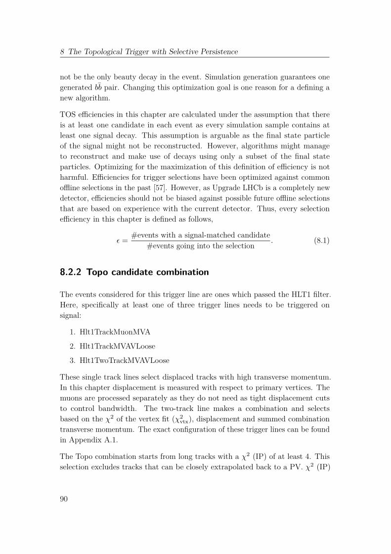
8 The Topological Trigger with Selective Persistence
not be the only beauty decay in the event. Simulation generation guarantees onegenerated 𝑏�̄� pair. Changing this optimization goal is one reason for a defining anew algorithm.
TOS efficiencies in this chapter are calculated under the assumption that thereis at least one candidate in each event as every simulation sample contains atleast one signal decay. This assumption is arguable as the final state particleof the signal might not be reconstructed. However, algorithms might manageto reconstruct and make use of decays using only a subset of the final stateparticles. Optimizing for the maximization of this definition of efficiency is notharmful. Efficiencies for trigger selections have been optimized against commonoffline selections in the past [57]. However, as Upgrade LHCb is a completely newdetector, efficiencies should not be biased against possible future offline selectionsthat are based on experience with the current detector. Thus, every selectionefficiency in this chapter is defined as follows,
𝜖 = #events with a signal-matched candidate#events going into the selection
. (8.1)
8.2.2 Topo candidate combination
The events considered for this trigger line are ones which passed the HLT1 filter.Here, specifically at least one of three trigger lines needs to be triggered onsignal:
1. Hlt1TrackMuonMVA
2. Hlt1TrackMVAVLoose
3. Hlt1TwoTrackMVAVLoose
These single track lines select displaced tracks with high transverse momentum.In this chapter displacement is measured with respect to primary vertices. Themuons are processed separately as they do not need as tight displacement cutsto control bandwidth. The two-track line makes a combination and selectsbased on the 𝜒2 of the vertex fit (𝜒2
vtx), displacement and summed combinationtransverse momentum. The exact configuration of these trigger lines can be foundin Appendix A.1.
The Topo combination starts from long tracks with a 𝜒2 (IP) of at least 4. Thisselection excludes tracks that can be closely extrapolated back to a PV. 𝜒2 (IP)
90

8.2 Optimization of the topological event selection
is calculated by calculating the 𝜒2 on a single iteration fit of the track onto theclosest primary vertex. It serves as measure for displacement from the beam.Tracks that come from beauty mesons mostly exhibit high 𝜒2 (IP) values becausethey extrapolate back to the displaced beauty decay vertex instead of any PV. Adistribution of 𝜒2 (IP) in 𝐵0
𝑠 → 𝜙𝜙 events can be seen in Figure 8.1.
0 5 10 15 202(IP)
10 2
10 1
arbi
trary
uni
tsfrom Bs
background
Figure 8.1: 𝜒2 (IP) distribution of long tracks in 𝐵0𝑠 → 𝜙𝜙 simulated events.
The orange distribution corresponds to tracks that do not originate from beautyhadrons. The blue distribution contains tracks which come from 𝐵0
𝑠 → 𝜙𝜙.
The tracks are transformed into particles and combined into B candidate. Thetwo-body combination is selected to have a distance of closest approach of less than1 mm. If the tracks do not extrapolate to a common point, it becomes much lesslikely that they originated from the same decay vertex. Because beauty mesonshave a relatively high mass, the combined transverse momentum of the tracksin the combination is expected to be larger than for the average combination oftracks. Therefore, a combined transverse momentum of over 1 GeV is required forthe two-body combination.
The candidates’ selection comprises the following requirements:
1. Flight distance 𝜒2 greater than 16. This indicates high displacement ofthe decay vertex and primary vertices. Because beauty hadrons have highlifetimes, this cut has high separation power.
2. cos(DirA) with respect to the closest PV greater than 0. DirAis the openingangle between the candidate momentum and the line between decay vertexand best PV. This value might differ from 0 significantly if not all tracksare captured by the combination. However, an angle over 90° is unlikely forsignal decays as this would imply a very large amount of missing momentum.
91

8 The Topological Trigger with Selective Persistence
3. Pseudorapidity of the interpolation between best PV and decay vertex withrespect to the beam line between 2 and 5. This is equivalent to the LHCbdetector acceptance. Almost every combination passes this cut.
To motivate the use of cos(DirA) and flight distance 𝜒2 in the preselection, thedistributions of these variables in 𝐵0
𝑠 → 𝜙𝜙 events are shown in Figures 8.2. Whilethe cuts are loose, they can already get rid of a large portion of the background.
0 10 20 30 40 50Flight distance 2
0.00
0.02
0.04
0.06
arbi
trary
uni
ts
signalbackground
1.0 0.5 0.0 0.5 1.0cos(DIRA)
0.0
2.5
5.0
7.5
10.0
12.5
15.0
arbi
trary
uni
ts
signalbackground
Figure 8.2: Flight distance 𝜒2 (left) and cos(DirA) (right) distributions two-body combinations in 𝐵0
𝑠 → 𝜙𝜙 simulated events. The blue distributioncorresponds to signal candidates, truth matched to the signal decay. Theorange distribution shows background candidates.
For the two-body selection, the Topo candidate is required to pass any of thepreviously listed HLT1 lines. TOS in single track lines is defined such thateither one of the tracks in the Topo candidate should have passed the linesrequirements.
The three-body combination builds upon the two-body combination. After anothercut on the two-body combination, 𝜒2
vtx smaller than 10, these are combined withanother charged basic particle. The three-body combination is required to havea combined transverse momentum of over 2 GeV. The same distance of closestapproach requirement and the same vertex cuts as in the two-body case areapplied. Again, at least one child has to pass one of the HLT1 trigger lines. Notethat the two-body combinations considered for the three-body combination donot need to pass the HLT1 lines by themselves, only in combination with thethird track.
92

8.2 Optimization of the topological event selection
Efficiencies for the outlined combination and selection are displayed in Table 8.1.The definition of the efficiencies is given in Section 8.2.1. Two-body decays like𝐵0 → 𝐾+𝜋− exhibit a lower efficiency due to combinatorial chance. Reconstruct-ing exactly the two right tracks is a two-body Topo is less likely than combiningtwo out of N for a N-body decay with N > 2.
Table 8.1: TOS efficiencies for the preselection.
Decay Efficiency [%]
𝐵0 → 𝐾+𝜋− 35.9𝐵0 → 𝐷+𝐷− 79.1𝐵0
𝑠 → 𝜙𝜙 73.7𝐵0 → 𝜋+𝜋−𝜋0 48.1𝐵0 → 𝐾∗(892)𝑒+𝑒− 63.6𝐵0 → 𝐷∗−𝜇+𝜈𝜇 33.0
𝐵0 → 𝐷∗−(𝜏+ → 3𝜋𝜈𝜏)𝜈𝜏 46.6𝐵0 → 𝐷∗−(𝜏+ → 𝜇+𝜈𝜇𝜈𝜏)𝜈𝜏 46.3
𝐵0𝑠 → 𝐷−
𝑠 𝐾+ 75.9Λ0
𝑏 → Λ+𝑐 𝐷−
𝑠 78.2
8.2.3 Boosted tree ensembles
The B candidate selection after reconstruction and combination is a multivariatebinary classification on a relatively small feature space. Ensemble methods,specifically Boosting, have proven to be very effective in these tasks. Gradientboosting algorithms have been dominating the Kaggle [81] classification scene forseveral years now. LHCb has a history of employing boosting for classificationtasks, mostly in data analyses. The in-house implementation of several MLalgorithms including boosted decision trees, TMVA [82], has been used for over adecade. Boosted trees have been used to train the topological selection for Run 2and we will continue to do so here.
The basics of boosting will shortly be outlined in the context of Classification AndRegression Tree (CART) ensembles. Firstly, a CART is a binary tree structure
93

8 The Topological Trigger with Selective Persistence
that splits inputs based on their properties, recursively. Figure 8.3 shows anexample tree with weights in the leaves. Regression trees have continuous andclassification trees have discrete output. An input to the tree will traverse it byapplying the selections defined in the nodes. If the input meets the requirement,it proceeds along a green arrow, otherwise a red. The output is the weight inthe leaf the input ends up in. If weights and criteria are well-adjusted, onecould interpret the output of this tree as an estimation for signal probability formuons from a B meson. By increasing the depth and the number of leaves, moresophisticated selections can be encoded in a decision tree. Trees are usually builtby iteratively introducing new nodes. In each step the criterion that can bestoptimize an objective function is chosen to form a new node. This is called greedyoptimization.
Muon?
0.2PT > 2 GeV
0.9 0.4
Figure 8.3: A simple tree with 3 leaves and a depth of 2. It assigns a numberto the input based on which leaf it ends up in. A green arrow corresponds to apass of the criterion defined by the node, a red arrow means fail.
To model more complex functions, a single tree needs a huge number of parameters.Because of this property, they are often referred to as ”weak learners”. This iswhere boosting algorithms come in. Instead of considering one tree, they buildensembles of trees, the weights of which are added to achieve arbitrarily goodfunction approximations. Most boosting algorithms iteratively fit weak learners torectify miss-predictions of the previous iteration. Gradient boosting will be usedin all new Topo implementations described in this chapter, so is quickly outlinedhere:
1. Training set: 𝑁 Samples and truth (𝑥𝑖, 𝑦𝑖 ∈ {−1, 1})2. A differential loss function 𝐿(𝑦, ̂𝑦).
94

8.2 Optimization of the topological event selection
3. Initialize the model 𝐹0(𝑥𝑖) = 𝑐𝑜𝑛𝑠𝑡.4. for 𝑘 = 1..𝐾
a) Compute residuals (errors) of the current model:
𝑘𝑖 = −∂𝐿(𝑦𝑖, 𝐹𝑘−1(𝑥𝑖))∂𝐹𝑘−1(𝑥𝑖)
b) Fit a weak learner ℎ𝑘(𝑥) to model the residuals.
c) Choose a weight 𝛾𝑘 to minimize the loss on the current model:
𝐿𝑘(𝑦, ̂𝑦) = ∑𝑖
𝐿(𝑦𝑖, (𝐹𝑘−1 + 𝛾𝑘ℎ𝑘)(𝑥𝑖))
d) Update the model 𝐹𝑘(𝑥) = 𝐹𝑘−1 + 𝛾𝑘ℎ𝑘(𝑥)
Gradient boosting can be interpreted as generalization to AdaBoost, the algorithmused in previous implementations of the Topo [83]. It uses an exponential lossfunction 𝐿(𝑦, ̂𝑦) = ∑𝑖 𝑒−𝑦𝑖⋅ ̂𝑦𝑖 . There are many parameters in a gradient boostingclassifier that can be tuned to increase performance. For instance, one can onlyconsider subsets of the data in each step, or use different factors 𝛾𝑘 to adjust howfast and how likely classifiers reach local minima.
8.2.4 Topological classification - Baseline comparison
The heart of the topological trigger is the multivariate selection that acts on thepreviously produced and selected Topo candidates. As opposed to other, exclusivetrigger lines, the selections described in Section 8.2.2 are very loose and yielda high output rate. The multivariate selection aims to optimize efficiency onreconstructed beauty decays while maintaining a relatively low output rate.
The Run 2 Topological trigger applies the multivariate classifier to each candidateindividually. The resulting trigger decision corresponds to whether at least one ofthe candidates passes the classification. The current baseline for the upgrade Topoas well as the first new implementation described here use the same workflow.A gradient boosting algorithm proves to be very efficient for the classificationtask.
As shortly discussed in Section 8.2.1, the training data for the baseline algorithmuses the ”FromSameB” definition for classification. If all children in the candidate
95

8 The Topological Trigger with Selective Persistence
are matched to a simulated basic particle that comes from the same simulated𝐵 hadron, a candidate is considered to be part of the signal data set. This doesnot necessarily need to be the signal hadron of the simulated sample. Although itincreases the statistical power of the signal data set, it does not fully represent themetric to optimize for, namely the efficiency of the signal decay. This is the firstof four motivations to train a new Topo classifier. The second motivation is theinput data. The baseline algorithm is trained on a smaller and less representativeinput collection. Thirdly, the input decay signatures are not weighted equally,but simply uniformly and thus proportionally to the different number of inputsamples available for each decay. Lastly, the TMVA implementation boostedtree ensembles trains rather slowly compared to modern implementations. Frompersonal experience, it requires significant manual tuning to reach competitiveperformance. Instead, the Catboost [84] library is employed for the new algorithms.During the course of these studies, Catboost and LightGBM [85] were comparedin different scenarios and with different hyperparameters and always yieldedvery similar results. Finally, Catboost was chosen because it has the option toexport most of their models to native Python and C++, which greatly eases theintegration into the LHCb software stack.
This section compares the different optimization methods and implementations.New algorithms are trained with the same signal definition as the baseline uses.Only the algorithms and data preprocessing cause performance differences.
In Section 8.2.5 algorithms are optimized for the selection of the signal decayitself.
Input data to the baseline approach comprises the following decays:
• 𝐵0 → (𝐷+ → 𝐾−𝜋+𝜋+)(𝐷− → 𝐾+𝜋−𝜋−)
• 𝐵0𝑠 → (𝜙 → 𝐾+𝐾−)(𝜙 → 𝐾+𝐾−)
• 𝐵0 → 𝜋+𝜋−(𝜋0 → 𝛾𝛾)
• 𝐵0𝑠 → (𝐷−
𝑠 → 𝐾+𝐾−𝜋−)𝐾+
• 𝐵0 → 𝑋𝑐𝜇𝜈𝜏
• Minimum bias
Each entry in the training sample comprises features presented in Table 8.2 andthe signal label. Distributions of three input features with high separation powerare shown for illustration in Figures 8.4. Signal in 𝐵0
𝑠 → 𝜙𝜙 events are plotted
96

8.2 Optimization of the topological event selection
against background candidates reconstructed in minimum bias events. Althoughthese features show significant differences in signal and background, they alsomotivate the use of a multivariate classifier. None of these features can be usedfor rectangular selections without sacrificing portions of the signal. The boostedtree ensemble will does a much better job of retaining signal while discardingbackground due to exploitation of correlations between these features.
0.988 0.990 0.992 0.994 0.996 0.998candidate cos(DIRA)
100
101
102
103
arbi
trary
uni
ts
From Bs
Background
0 50 100 150 200candidate vertex 2
10 5
10 4
10 3
10 2
10 1
arbi
trary
uni
ts
From Bs
Background
500 1000 1500track minimum 2(IP)
10 4
10 3
10 2
arbi
trary
uni
ts
From Bs
Background
Figure 8.4: Distributions of candidate cos(DIRA), vertex 𝜒2 and track mini-mum 𝜒2(IP) for 𝐵0
𝑠 → 𝜙𝜙 signal candidates versus minimum bias background.
To measure and compare performances of different classifying solutions, the TruePositive Rate (TPR) is plotted against the False Positive Rate (FPR). This isknown as Receiver Operator Characteristic (ROC) and is a commonly used forperformance visualization in binary classification tasks because it is independentof the number of background and signal samples and their ratio. The area underthat curve (AUC) can give a single number score without the need to choose a cutpoint. For final evaluation, several realistic cut points will be chosen to measureefficiency given output rate.
The baseline implementation used the AdaBoost implementation in TMVA with100 weak learners. The new models use gradient boosting on binary cross-entropy
97

8 The Topological Trigger with Selective Persistence
Table 8.2: Input features to the Topo training
Feature Explanation
(2,3)-Body CORRM Corrected invariant mass √𝑀2 + (𝑝𝑚𝑇 )2 + 𝑝𝑚
𝑇 . 𝑝𝑚𝑇 is
the missing transverse momentum to match the mo-mentum vector and the linear extrapolation betweencorresponding PV and decay vertex.
(2,3)-Body DOCAMAX Maximum distance of closest approach between chil-dren.
(2,3)-Body FD 𝜒2 Measure for displacement of decay (𝑑) and primary(𝑝) vertex: ( ⃗𝑥𝑑 − ⃗𝑥𝑝)𝑇(cov𝑑 + cov𝑝)( ⃗𝑥𝑑 − ⃗𝑥𝑝), wherecov𝑑(𝑝) are the covariance matrices for decay or pri-mary vertex position.
(2,3)-Body P(T) (transverse) momentum of the reconstructed mother(2,3)-Body cos(DIRA) cos of the direction angle of the reconstructed mother
with respect to the PV(2,3)-Body 𝜒2 (IP) 𝜒2 (IP) of the reconstructed mother(2,3)-Body 𝜒2
vtx 𝜒2vtx of the reconstructed mother
child 𝜒2 (IP) 𝜒2 (IP) of the childrenchild P(T) (transverse) momentum of the children
loss with up to 3000 weak learners. With such a large number of weak learners,overtraining might become a problem. Overtraining names the phenomenon wherea model becomes sensitive to the statistical fluctuations of its training data, thuslacks generalization and performs much worse on unseen samples.
Four methods are employed to counter overtraining: Firstly, a threefold crossvalidation is used. The data is split three-way, and training is performed on twothirds while validation happens on the third, unseen sample. This is done thrice,each time with a different third as validation sample. The model is considered fineif all three resulting models behave similarly. Secondly, the L2 generalization termin the loss function adaptively reduces the weights in the leaves when they getmuch larger than average. Thirdly, a technique called early stopping constraintsthe number of weak learners. When the model does not continue improving onthe validation set, early stopping will stop the training progress and effectively
98

8.2 Optimization of the topological event selection
reduce the number of weak learners. Lastly, the random subspacing helps withgeneralization because the model is forced to consider not only the features thatappear very predictive on the training set.
Considering multiple candidates in a Topo event at once might yield more ex-ploitable correlations for the classification algorithm. Therefore, a second trainingworkflow was considered: Use the three candidates with the highest predictionin the previously trained model as one input sample to get a better event wisediscrepancy. This workflow yields an event wise prediction, while the other config-urations yield candidate wise predictions. The problem with event wise decisions isthat a TOS efficiency cannot be defined. However, the classification performancecan still be compared when ignoring the TOS requirement. To do so, candidatepredictions are translated to event predictions by taking the highest prediction ofall candidates in the event. An event wise label is defined as whether at least onecandidate is present in it. Note that the approach with the three best candidatesis not pursued further within this thesis as the final goal is defined to be TOSefficiency. It rather serves as showcase for the fact that information besides thesignal candidate helps in selecting signal events more efficiently.
As both two- and three-body classification should run in the trigger, the importantmetric to compare is the combined performance. Therefore, predictions on bothdatasets are combined by taking the maximum prediction of any two- or three-body candidate within the event. This maximum aggregation is only negligiblyworse than a brute force threshold optimization for best efficiency given fixedoutput rate in a two-dimensional space. The combined performance for baselineand new models is compared in Figures 8.5.
The data used for these scores represents a slice of the input data that has not beenseen by any of the new models trained within the cross validation scheme. Becausethree models have been trained during cross validation, the unseen data will beclassified by taking the mean prediction of all three models. Averaging ratherthan predicting with one model changes the scores negligibly, which suggests thatgeneralization works well. Each plot presents a specific input decay for signal, butalways minimum bias data for the background.
The comparison plots suggest that the newly trained models perform betterin the general case. Specifically the 𝐵0
𝑠 → 𝜙𝜙 and 𝐵0 → 𝜋+𝜋−𝜋0 decays arecaptured up to factors of 2 better, depending on the output bandwidth. The𝐵0 → 𝐷+𝐷− sample is a factor 3 larger than all others. Overtraining mightexplain the performance differences over the samples. It is also apparent that
99

8 The Topological Trigger with Selective Persistence
considering multiple candidates in an event wise decision generally outperformsthe simple maximum aggregation that the default Topo algorithm employs.
Note that Figures 8.5 show the classification performance in terms of the ”From-SameB” definition, but these do not necessarily reflect the signal efficiency asdefined in Section 8.2.1. Figures 8.6 therefore show signal efficiency given outputrate relative to the input rate. Here, every simulated signal event is counted assignal since the simulation guarantees at least one signal decay in each simulatedevent. The rate is estimated on minimum bias events. One can see that theincreased performance of the new algorithms is reflected in higher signal efficiencyper output rate.
8.2.5 Topological classification - Full input data
The new models showing improved performance can now be applied to the widerinput decay selection described in section 8.1. The training in this chapteroptimizes TOS efficiency of signal events as defined in 8.2.2. Samples are weightedto ensure balance between the different samples. The performance of the combinedtwo- and three-body classification algorithms given a minimum bias output ratecan be seen in Figures 8.7.
The output bandwidth envisioned for the Topo amounts to 3 GB/s [83]. Toestimate bandwidths given selection efficiencies, multiple factors need to bedetermined. The output bandwidth of the default Topo is determined as follows:
𝑏(𝑡) = 𝑟(𝑡) ⋅ 𝛽(𝑡) (8.2)
where 𝑏 is the bandwidth, 𝑟 the output rate, 𝑡 the threshold configuration and 𝛽the average bandwidth per minimum bias event that passes the Topo selection.Because the number of Topo candidates vary with the thresholds, 𝛽 is a functionof 𝑡. To determine 𝛽(𝑡), the bandwidth of all pieces of information to be persistedhave to be assessed. In the default persistence setting where all information ofthe event has to be persisted, 𝛽 comprises the following parts:
𝛽(𝑡) = 𝛽downstream + 𝛽upstream + 𝛽neutrals + 𝛽long + 𝛽topo(𝑡) (8.3)
The contributors to bandwidth are downstream, upstream and long tracks andneutral particles. Additionally, each reconstructed Topo candidate has someinformation to be persisted. The output bandwidth of each contributor has been
100

8.2 Optimization of the topological event selection
estimated by running the baseline Topo as defined in 8.2.4. The persisted size offinal state particles is determined to be
𝛽downstream = 10.2 kB, (8.4)𝛽upstream = 11.5 kB, (8.5)𝛽neutrals = 13.8 kB, (8.6)
𝛽long = 55 kB. (8.7)
These numbers represent an average size of all tracks of the specified type in anevent. As the number of Topo candidates depends on the threshold configuration,the size of these are determined on a per-candidate basis:
𝛽topo(𝑡) = 𝛽topocandidate ⋅ 𝑛topo
candidate(𝑡) = 360 B ⋅ 𝑛topocandidate(𝑡), (8.8)
where 𝑛topocandidate is the average number of Topo candidates per event, which depends
on the selection thresholds. Thresholds are optimized for highest average TOSefficiency over the input samples given the bandwidth limit of 3 GB/s. Table 8.3shows the TOS efficiencies given these thresholds.
Table 8.3: TOS efficiencies for Topo classifiers. For a total efficiency, theseare to be multiplied with the preselection efficiencies in 8.1.
Decay Efficiency [%]
𝐵0 → 𝐾+𝜋− 92.2𝐵0 → 𝐷+𝐷− 35.4𝐵0
𝑠 → 𝜙𝜙 75.6𝐵0 → 𝜋+𝜋−𝜋0 55.3𝐵0 → 𝐾∗(892)𝑒+𝑒− 56.0𝐵0 → 𝐷∗−𝜇+𝜈𝜇 43.3
𝐵0 → 𝐷∗−(𝜏+ → 3𝜋𝜈𝜏)𝜈𝜏 26.2𝐵0 → 𝐷∗−(𝜏+ → 𝜇+𝜈𝜇𝜈𝜏)𝜈𝜏 26.8
𝐵0𝑠 → 𝐷−
𝑠 𝐾+ 53.1Λ0
𝑏 → Λ+𝑐 𝐷−
𝑠 38.0
101

8 The Topological Trigger with Selective Persistence
0.0 0.2 0.4 0.6 0.8 1.0False positive rate
0.0
0.2
0.4
0.6
0.8
1.0
True
pos
itive
rate
B0 D + D
baseline, ROC AUC: 0.970per candidate, ROC AUC: 0.960three best, ROC AUC: 0.968Random choice
0.0 0.2 0.4 0.6 0.8 1.0False positive rate
0.0
0.2
0.4
0.6
0.8
1.0
True
pos
itive
rate
B0 Xc
baseline, ROC AUC: 0.937per candidate, ROC AUC: 0.935three best, ROC AUC: 0.950Random choice
0.0 0.2 0.4 0.6 0.8 1.0False positive rate
0.0
0.2
0.4
0.6
0.8
1.0
True
pos
itive
rate
B0s
baseline, ROC AUC: 0.947per candidate, ROC AUC: 0.967three best, ROC AUC: 0.975Random choice
0.0 0.2 0.4 0.6 0.8 1.0False positive rate
0.0
0.2
0.4
0.6
0.8
1.0Tr
ue p
ositi
ve ra
teB0 + 0
baseline, ROC AUC: 0.846per candidate, ROC AUC: 0.929three best, ROC AUC: 0.950Random choice
0.0 0.2 0.4 0.6 0.8 1.0False positive rate
0.0
0.2
0.4
0.6
0.8
1.0
True
pos
itive
rate
B0s Ds K +
baseline, ROC AUC: 0.929per candidate, ROC AUC: 0.946three best, ROC AUC: 0.959Random choice
Figure 8.5: ROC curves and scores for the baseline Topo classifiers and thenew models trained on the same input data. The plots differ only by thesignal sample considered. Each plot considers the classification of one of theinput samples against minimum bias background. Blue represents the baselinemodel. Orange and green curves represent two different training methodsemployed to train the new models. The blue and orange models are trained ona per-candidate basis.
102

8.2 Optimization of the topological event selection
0.0 0.2 0.4 0.6 0.8 1.0output rate fraction
0.0
0.2
0.4
0.6
0.8
1.0
signa
l effi
cienc
y
B0 D + D
baselineper candidatethree bestRandom choice
0.0 0.2 0.4 0.6 0.8 1.0output rate fraction
0.0
0.2
0.4
0.6
0.8
1.0
signa
l effi
cienc
y
B0 Xc
baselineper candidatethree bestRandom choice
0.0 0.2 0.4 0.6 0.8 1.0output rate fraction
0.0
0.2
0.4
0.6
0.8
1.0
signa
l effi
cienc
y
B0s
baselineper candidatethree bestRandom choice
0.0 0.2 0.4 0.6 0.8 1.0output rate fraction
0.0
0.2
0.4
0.6
0.8
1.0
signa
l effi
cienc
yB0 + 0
baselineper candidatethree bestRandom choice
0.0 0.2 0.4 0.6 0.8 1.0output rate fraction
0.0
0.2
0.4
0.6
0.8
1.0
signa
l effi
cienc
y
B0s Ds K +
baselineper candidatethree bestRandom choice
Figure 8.6: Signal efficiency against output event rate using combined two-and three-body event predictions. Signal efficiency is here defined as the numberof events of the signal decay samples passing the selection. Background isdefined by the fraction of minimum bias events that pass.
103

8 The Topological Trigger with Selective Persistence
102
101
100
output rate fraction
0.2
0.4
0.6
0.8
1.0signal efficiency
Random choice
B0s
Ds
K+
B0
D+
DB
0s
B0
K+
B0
D0
B0
D*(
3)
B0
D*(
)B
0K
*e+
eB
0+
0
bc D
s
Figure
8.7:T
OS
signalefficiency
againstoutput
eventrate
usingcom
binedtwo-and
three-bodyeventpredictionsforallinputsam
plesusingthe
maxim
umoftw
o-andthree-body
prediction.T
hex-axis
isin
logarithmic
scale.
104

8.3 Selective Persistence in the topological trigger
8.3 Selective Persistence in the topological trigger
The goal of this chapter is the reduction of persisted size of an event selectedby the topological trigger. This can be achieved via Selective Persistence (SP)as opposed to the Full Persistence (FP). Selective Persistence in exclusive lineshas been utilized for several operational years now. Line developers in Run 2 hadthe option to persist anything between only the candidate decay chain to theentire event, depending on physics analysis needs. Figure 8.8 sketches the possiblechoices and their impact on output bandwidth.
Figure 8.8: Different choices for signal event persistence. The minimumneeded is the signal candidate and its children. One can optionally save morerelated information up to every signature in the event [86].
105

8 The Topological Trigger with Selective Persistence
Employing SP on the Topo output is significantly harder for two reasons. Firstly,the inclusive nature of this line implies that it is supposed to be used for manydifferent analyses. Therefore, a definition of relevant information for offline usemight be too restrictive. Secondly, the decay signatures selected by the Topoare often more than the reconstructed two- and three-body candidates used forthe actual selection. Unlike in an exclusive line, the decay chain itself is notspecified.
To address the first problem, the following assumption will be made: Relevantinformation for offline analyses concerns trajectories that come from a beautydecay chain. This implies the tracks that come from the other beauty quarkin the 𝑏�̄� pair production. Due to the many degrees of freedom and unknownsin a 𝑝𝑝-interaction, information that is not part of the 𝑏�̄� pair final states isuncorrelated to the beauty decay chain and can therefore not contribute any moreinformation to the signal decay. The approach of trying to select all trajectoriescoming from beauty decays automatically tackles the second problem as well, asthese tracks are a superset of the tracks coming from the signal beauty hadron.
The problem now reduces to: How can one efficiently select these tracks? Twoapproaches are discussed here.
Selection based on primary vertex relations
The simplest idea utilizes the fact that in the typical upgrade event there aremore than one primary interaction point. However, the 𝑏�̄� pair of interest mayonly produce tracks that either extrapolate back to that PV very precisely ortracks that come from a displaced decay vertex. The sketch in Figure 8.8 displaysthis. As displacement of tracks is measured by minimum distance to any of thePVs, a problem arises when displaced tracks extrapolate towards a different fromtheir actual PV by chance. Concretely, the tested selection criterion to selecttracks is build as follows: Take any track that extrapolates back to the sameprimary vertex as the Topo candidate with a small impact parameter to that PV.Additionally, take all sufficiently displaced vertices as defined by the minimumimpact parameter with respect to all PVs. The performance of this approach canbe measured as every classification problem: A class probability is assigned basedon the outlined logic. The signal probability is assigned as follows:
𝑝1 = min(1, 𝛿(PV(track), PV(candidate)) + √𝜒2(IP)(track)/100), (8.9)
106

8.3 Selective Persistence in the topological trigger
where �represents the Kronecker delta. The PV function yields the best PV for agiven candidate or track. Conceptually this function should assign high values toprompt tracks from the same PV as the candidate and displaced tracks of all sorts.The scaling factor of 100 is chosen rather arbitrarily and defines the maximum𝜒2 (IP) for which the prediction still differs. Everything above an IP of 100 mmwill just be clipped to 1. Because a classification task only depends on differencesin predictions rather than the absolute value, the specific choice for the scalingfactor makes little to no difference as long as it is much larger than a commonvalue for prompt tracks, because otherwise even prompt tracks might yield a highprediction. The square root as monotonic function makes no theoretical difference.It helps when binning the 𝜒2 distribution as is done for the performance plots.
With a floating point prediction and truth values for whether a track originatesfrom a beauty decay, a signal efficiency vs. average retention fraction plot givesinformation about the prediction quality for all possible working points. Theaverage retention fraction is estimated on minimum bias samples while the signalefficiency is based on the respective signal sample. These curves for the differentdecays in the input samples are shown in Figures 8.9. Note that the calculationof 𝑝1 may be performed multiple times per track in each event, as it has tobe done for every Topo candidate. For a per-track prediction, the maximumvalue over all Topo candidates in the event is chosen. Specifically, if two- andthree-body selections yield Topo candidates in the same event, the maximum istaken over both types of candidates. Note also that events with more than one𝑏�̄� are discarded from the evaluation. The point of this study is to capture thetracks coming from the 𝑏�̄� pair the Topo candidate refers to.
A high per-track efficiency might not be good enough if one of the tracks that wasnot selected carried the crucial information. Therefore, all performance plots inthis section show a second curve made from a per-event prediction. By assigningan event the minimum prediction value of all signal tracks, we can estimatethe fraction of events where all relevant tracks are being selected with a giventhreshold. Notably, tracks which are part of any Topo candidate are alwaysselected. This explains the offset at the lower left of the performance plots.
Selection based on trained classification
A trained multivariate classifier usually performs better than a manually definedprediction as Equation (8.9). To train such a classifier, features from tracks and
107

8 The Topological Trigger with Selective Persistence
0.0 0.2 0.4 0.6 0.8 1.0fraction of accepted tracks [%]
0.0
0.2
0.4
0.6
0.8
1.0
signa
l effi
cienc
y [%
]
B0 K +
all signal in event selectedper track efficiency
0.0 0.2 0.4 0.6 0.8 1.0fraction of accepted tracks [%]
0.0
0.2
0.4
0.6
0.8
1.0
signa
l effi
cienc
y [%
]
B0 + 0
all signal in event selectedper track efficiency
0.0 0.2 0.4 0.6 0.8 1.0fraction of accepted tracks [%]
0.0
0.2
0.4
0.6
0.8
1.0
signa
l effi
cienc
y [%
]
B0 K * e + e
all signal in event selectedper track efficiency
0.0 0.2 0.4 0.6 0.8 1.0fraction of accepted tracks [%]
0.0
0.2
0.4
0.6
0.8
1.0
signa
l effi
cienc
y [%
]
B0 D * ( 3 )
all signal in event selectedper track efficiency
Figure 8.9: Prediction performance of 𝑝1, visualized via long track acceptancefraction vs. efficiency for combined two- and three-body selections. The orangecurve displays the fraction of tracks from beauty decay chains that are acceptedby the classifier given a total track retention. The blue curve shows the fractionof events where all tracks from beauty decay chains were captured.
108

8.3 Selective Persistence in the topological trigger
0.0 0.2 0.4 0.6 0.8 1.0fraction of accepted tracks [%]
0.0
0.2
0.4
0.6
0.8
1.0
signa
l effi
cienc
y [%
]
B0 D + D
all signal in event selectedper track efficiency
0.0 0.2 0.4 0.6 0.8 1.0fraction of accepted tracks [%]
0.0
0.2
0.4
0.6
0.8
1.0
signa
l effi
cienc
y [%
]
B0 D * ( )
all signal in event selectedper track efficiency
0.0 0.2 0.4 0.6 0.8 1.0fraction of accepted tracks [%]
0.0
0.2
0.4
0.6
0.8
1.0
signa
l effi
cienc
y [%
]
B0 D0
all signal in event selectedper track efficiency
0.0 0.2 0.4 0.6 0.8 1.0fraction of accepted tracks [%]
0.0
0.2
0.4
0.6
0.8
1.0
signa
l effi
cienc
y [%
]B0
s
all signal in event selectedper track efficiency
0.0 0.2 0.4 0.6 0.8 1.0fraction of accepted tracks [%]
0.0
0.2
0.4
0.6
0.8
1.0
signa
l effi
cienc
y [%
]
B0s Ds K +
all signal in event selectedper track efficiency
0.0 0.2 0.4 0.6 0.8 1.0fraction of accepted tracks [%]
0.0
0.2
0.4
0.6
0.8
1.0
signa
l effi
cienc
y [%
]
b cDs
all signal in event selectedper track efficiency
Figure 8.9: Prediction performance of 𝑝1, visualized via long track acceptancefraction vs. efficiency for combined two- and three-body selections. The orangecurve displays the fraction of tracks from beauty decay chains that are acceptedby the classifier given a total track retention. The blue curve shows the fractionof events where all tracks from beauty decay chains were captured.
109

8 The Topological Trigger with Selective Persistence
Topo candidates can be extracted to base a prediction 𝑝2 on. A selection basedsolely on track features has briefly been explored to yield non-competitive results,and is therefore not further described here. Instead, the data is prepared bycombining each Topo candidate that comes out of the topological trigger line andits own classifier with each track in an event. For each of these combinations,features to base the classification on can be determined. The relevant ones includefeatures related to the candidate, the track, the combination of both and theprimary vertices. Specifically, the features described in Table 8.4 are used forclassification training. Note that two types of classifiers are trained, becausefeatures for two- and three-body Topo candidates come with different featuresused in the classifier. The gradient boosting implementation in LightGBM isused as it trains faster in a CPU environment with the type of data used here.Classification performances of Catboost and LightGBM implementations yieldnegligible differences. For final integration into the LHCb software stack, one mayswitch back to Catboost for easy translation to C++. All previously outlinedmeasures to counter overtraining are taken here as well.
The performance plots for the combined predictions given by both classificationalgorithms is shown in Figures 8.10. The overall superiority of the trainedclassification is apparent. Using the shown method of selectively persisting tracksin the Topo trigger line enables one of two things: Either the Topo output rate canbe increased to yield a higher overall signal efficiency or the freed up bandwidthmay be used for other lines struggling with output rate control. For a 50% trackretention working point the event loss would stay under 5% in all signal decaysamples, even in the worst case scenario where only those events are usable inwhich all tracks from beauty decay chains have been captured by the classifier.One can use these bandwidth reductions to change thresholds of the Topo selection.The efficiency gain is visible in Table 8.3. Otherwise, the freed up bandwidthcould be used to ease requirements on other important trigger lines. A globaloptimization has to be conducted to determine a good trade-off for all physicsinterests the trigger has to cover.
When removing 50% of the long tracks the Topo thresholds can be adjusted toincrease the overall efficiencies of the signal decays, unless the freed up bandwidthis used in other trigger lines. Efficiencies for thresholds in both scenarios areshown in Table 8.5, once with and once without discarding 50% of the long tracks.The thresholds are optimized for highest TOS efficiency within the bandwidthlimit.
110

8.3 Selective Persistence in the topological trigger
0.0 0.2 0.4 0.6 0.8 1.0fraction of accepted tracks [%]
0.0
0.2
0.4
0.6
0.8
1.0
signa
l effi
cienc
y [%
]
B0 K +
all signal in event selectedper track efficiency
0.0 0.2 0.4 0.6 0.8 1.0fraction of accepted tracks [%]
0.0
0.2
0.4
0.6
0.8
1.0
signa
l effi
cienc
y [%
]
B0 + 0
all signal in event selectedper track efficiency
0.0 0.2 0.4 0.6 0.8 1.0fraction of accepted tracks [%]
0.0
0.2
0.4
0.6
0.8
1.0
signa
l effi
cienc
y [%
]
B0 K * e + e
all signal in event selectedper track efficiency
0.0 0.2 0.4 0.6 0.8 1.0fraction of accepted tracks [%]
0.0
0.2
0.4
0.6
0.8
1.0
signa
l effi
cienc
y [%
]
B0 D * ( 3 )
all signal in event selectedper track efficiency
Figure 8.10: Prediction performance of 𝑝2, equivalent to Figures 8.9.
111
8 The Topological Trigger with Selective Persistence
Table 8.4: Input features to the track classification training
Feature Explanation
Topo-Track-DOCA (𝜒2) Distance (𝜒2) of closest approach between the candi-date and the track
Topo-Track-P(T) (Transverse) Momentum of the combined Topo andtrack candidate.
Topo-Track-𝜂 Pseudorapidity of the combined Topo and track can-didate.
Topo-Track-𝜒2vtx 𝜒2
vtx of the Topo and track candidate if a vertex fitbetween them converged, otherwise an error value.
Topo-Track-IP (𝜒2) Impact Parameter (𝜒2) between Topo candidate andtrack.
Topo-Track-𝛥𝑅2 𝛥𝜂2 + 𝛥𝜙2 between Topo and track. 𝜙 is the anglein the x-y-plane of the detector
(2,3)-Body DOCA 𝜒2 Maximum distance of closest approach 𝜒2 betweenchildren.
(2,3)-Body FD 𝜒2 Measure for displacement of decay and primary ver-tex.
(2,3)-Body MIP Minimum IP of Topo candidate with respect to PVs.(2,3)-Body VZ z-position of associated primary vertex.(2,3)-Body 𝜒2
vtx 𝜒2vtx of the Topo candidate.
(2,3)-Body PRED Topo classifcation prediction.Track P(T) Track (transverse) momentum.Track 𝜂 Track pseudorapidity.Track MIP (𝜒2) Impact Parameter (𝜒2) between track and its associ-
ated primary vertex.Track 𝜒2 𝜒2 of the track fit.Track GHOSTPROB Predicted probability for the track being a ghost.
This is determined by a neural network.
112

8.3 Selective Persistence in the topological trigger
0.0 0.2 0.4 0.6 0.8 1.0fraction of accepted tracks [%]
0.0
0.2
0.4
0.6
0.8
1.0
signa
l effi
cienc
y [%
]
B0 D + D
all signal in event selectedper track efficiency
0.0 0.2 0.4 0.6 0.8 1.0fraction of accepted tracks [%]
0.0
0.2
0.4
0.6
0.8
1.0
signa
l effi
cienc
y [%
]
B0 D * ( )
all signal in event selectedper track efficiency
0.0 0.2 0.4 0.6 0.8 1.0fraction of accepted tracks [%]
0.0
0.2
0.4
0.6
0.8
1.0
signa
l effi
cienc
y [%
]
B0 D0
all signal in event selectedper track efficiency
0.0 0.2 0.4 0.6 0.8 1.0fraction of accepted tracks [%]
0.0
0.2
0.4
0.6
0.8
1.0
signa
l effi
cienc
y [%
]
B0s
all signal in event selectedper track efficiency
0.0 0.2 0.4 0.6 0.8 1.0fraction of accepted tracks [%]
0.0
0.2
0.4
0.6
0.8
1.0
signa
l effi
cienc
y [%
]
B0s Ds K +
all signal in event selectedper track efficiency
0.0 0.2 0.4 0.6 0.8 1.0fraction of accepted tracks [%]
0.0
0.2
0.4
0.6
0.8
1.0
signa
l effi
cienc
y [%
]
b cDs
all signal in event selectedper track efficiency
Figure 8.10: Prediction performance of 𝑝2, equivalent to Figures 8.9.
113

8 The Topological Trigger with Selective Persistence
Table 8.5: TOS efficiencies for Topo classifiers given different bandwidthscenarios. For a total efficiency, these are to be multiplied with the preselectionefficiencies in 8.1. The left column is the same as in Table 8.3
Decay Efficiency [%] Efficiency [%]@ 100% persistence @ 50% long tracks
𝐵0 → 𝐾+𝜋− 92.2 93.2𝐵0 → 𝐷+𝐷− 35.4 42.8𝐵0
𝑠 → 𝜙𝜙 75.6 79.9𝐵0 → 𝜋+𝜋−𝜋0 55.3 62.1𝐵0 → 𝐾∗(892)𝑒+𝑒− 56.0 62.8𝐵0 → 𝐷∗−𝜇+𝜈𝜇 43.3 50.9
𝐵0 → 𝐷∗−(𝜏+ → 3𝜋𝜈𝜏)𝜈𝜏 26.2 36.2𝐵0 → 𝐷∗−(𝜏+ → 𝜇+𝜈𝜇𝜈𝜏)𝜈𝜏 26.8 36.6
𝐵0𝑠 → 𝐷−
𝑠 𝐾+ 53.1 58.0Λ0
𝑏 → Λ+𝑐 𝐷−
𝑠 38.0 46.3
114

8.4 Summary and outlook
8.4 Summary and outlook
This Chapter presented an optimized two- and three-body Topo classificationalgorithm to efficiently select a broad range of signal decay channels. It optimizesTOS efficiency as opposed to overall signal efficiency, because analysts prefer TOSselections to be able to model backgrounds accurately.
The Topo traditionally persisted all reconstructed information in an event becausethe usual implementation of SP is dependent on a fully known reconstructeddecay. In an inclusive line like the Topo, SP is much harder. One wants togeneralize over multiple decay channels, so any SP approach has to do the same.To try to reduce the output bandwidth per retained event, an approach for SPusing PV association was proposed. Because this approach shows significantlosses even at a high track retention, a second algorithm was proposed to performSP. A classification algorithm that predicts whether tracks come from a beautydecay chain is employed. This algorithm can discard 50% of all long trackswhile retaining a close to 100% efficiency. With the freed up bandwidth, one caneither enable other physics selections in the HLT2 or increase the efficiency of theTopo.
However, SP has only been tried on long tracks as these are the biggest contributorsto bandwidth. The next step is to evaluate the given method on upstream tracks.As these also exhibit VELO tracks, the topological information close to the decayvertex can be used in the same way as with long tracks. Downstream tracks andneutral particles will need to be handled differently. For Downstream tracks onemight select based on whether they combine to a 𝐾0
S or a 𝛬 particle. Under therough assumption that 50% of all particle and track types can be discarded withminimal loss, the efficiencies under the 3 GB/s bandwidth constraint would look asshown in Table 8.6. Larger efficiency improvements can be achieved in decays witha lower Topo efficiency. For instance, the efficiency of 𝐵0 → 𝐷∗−(𝜏+ → 3𝜋𝜈𝜏)𝜈𝜏decays could increase by almost a factor of two.
115

8 The Topological Trigger with Selective Persistence
Table 8.6: TOS efficiencies for Topo classifiers for all scenarios. The firstscenario assumes full persistence of all basics. The second scenario assumesthat 50% of all long tracks are discarded. The rightmost scenario assumes that50% of all basic particles can be removed with small loss.
Decay Efficiency [%] Efficiency [%] Efficiency[%]@ 100% persist. @ 50% long tracks @ 50% all basics
𝐵0 → 𝐾+𝜋− 92.2 93.2 93.7𝐵0 → 𝐷+𝐷− 35.4 42.8 51.4𝐵0
𝑠 → 𝜙𝜙 75.6 79.9 82.6𝐵0 → 𝜋+𝜋−𝜋0 55.3 62.1 65.9𝐵0 → 𝐾∗(892)𝑒+𝑒− 56.0 62.8 68.5𝐵0 → 𝐷∗−𝜇+𝜈𝜇 43.3 50.9 57.3
𝐵0 → 𝐷∗−(𝜏+ → 3𝜋𝜈𝜏)𝜈𝜏 26.2 36.2 48.3𝐵0 → 𝐷∗−(𝜏+ → 𝜇+𝜈𝜇𝜈𝜏)𝜈𝜏 26.8 36.6 46.7
𝐵0𝑠 → 𝐷−
𝑠 𝐾+ 53.1 58.0 62.2Λ0
𝑏 → Λ+𝑐 𝐷−
𝑠 38.0 46.3 55.6
116

9 Conclusion
LHCb is currently performing a significant detector upgrade involving a five-foldincrease of instantaneous luminosity and the removal of the hardware trigger stage.The work presented in this thesis tackles some of the challenges implied by thesechanges. Specifically, two challenges are addressed: Firstly, the event throughputof the current HLT application is factors too low to be processing 30 MHz of inputrate efficiently within the given budget. Secondly, LHCb needs to fit its broadphysics program into an output bandwidth limit of 10 GB/s.
The first contribution described in this thesis is the implementation of the firstfeature-complete scheduling algorithm that is fast enough to run in the productionenvironment without causing significant overheads to the application. Staticscheduling logic is prepared before event evaluation and runtime decisions arelimited to an absolute minimum. The algorithm can operate arbitrary controlflow and implements a barrier concept to be able to share work between algorithminstances. This scheduling algorithm marks an important contribution to the firstfully functioning HLT1 implementation. It is also the new baseline implementationfor the Upgrade HLT2 solution.
The second contribution is the renewal of the selection framework in HLT2. Algo-rithms needed for decay chain reconstruction after trajectory reconstruction proveto be one of the major bottlenecks for the HLT2 application throughput. About1000 different selection sequences will be using these algorithms in production.By overhauling the selection system and the particle event model, new implemen-tations described in this thesis achieve up to 10-fold throughput improvementsin decay chain reconstruction and particle selections. The transition to thesealgorithms in production will reduce the contribution of selection lines in HLT2to under 5% relative contribution.
The third contribution tackles the second big challenge of the Upgrade HLT: Theoutput bandwidth. With the constraint of 10 GB/s output bandwidth to perma-nent storage, many trigger lines have to transition to a selective persistence model.The Topological beauty selection is an inclusive trigger line with exceptionally high
117

9 Conclusion
bandwidth requirements. Due to its inclusive nature it cannot apply the usualmethods of selective persistence. Methods of optimizing the Topo selection toeither lower bandwidth requirements or increase efficiency are explored. Selectivepersistence can be applied by classifying tracks based on whether they originatefrom a beauty flavored particle. At more than 95% worst-case efficiency, 50% ofthe long tracks in an event can be removed to lower output bandwidth or increaseefficiency accordingly.
Summarized, crucial contributions for the operation of an efficient, fully softwarebased HLT were presented. As such, they mark important milestones towards thecollection of data corresponding to 50/fb integrated luminosity with unprecedentedefficiencies in beauty and charm decay channels.
To showcase the statistical power of the dataset to be collected in the next 10years, we compare efficiencies and production rates in several channels that wereconsidered throughout the thesis. Statistical uncertainties in measurements atLHCb usually scale roughly with the square root of the number of signal eventsretained. The 50/fb dataset already increases the amount of produced beautyand charm hadrons by more than a factor of 6 with respect to the Run 1 and2 datasets. For muonic channels like 𝐵0 → 𝐾∗𝜇+𝜇− and 𝐵0 → 𝐷∗−𝜇+𝜈 whichexhibit high efficiencies in both datasets, this corresponds to a factor of at least√
6 improvement in statistical sensitivity.
For channels involving electrons, like 𝐵0 → 𝐾∗𝑒+𝑒−, the sensitivity is furtherimproved due to the increased efficiency that the hardware trigger removal yields.In this case, the efficiency with and without the hardware trigger differs by abouta factor of two. The efficiency increase is most pronounced in channels with purelyhadronic final states like 𝐵0
𝑠 → 𝜙𝜙, 𝐵0 → 𝐷+𝐷− and 𝐵0 → 𝐷∗−(𝜏+ → 3𝜋𝜈𝜏)𝜈𝜏,where improvements of up to factors of 4 due to the removal of the hardwaretrigger are expected. This translates to another factor of
√2 − 2 in sensitivity.
The optimization of the Topo further increases the signal efficiency by itself, evenmore so if the bandwidth reduction due to selective persistence is utilized to retaina higher rate of events. This leads to further efficiency improvements of up to50 %.
To complete the Upgrade trigger, several open tasks remain. Most importantly,the HLT2 reconstruction has to be sped up by about a factor of two to be ableto process the HLT1 output rate. Secondly, the new selection framework hasto be completed and validated carefully for different decay scenarios to ensure
118

correctness. While there are several other details to be solved in both HLT1 andHLT2, I am confident that the LHCb collaboration will successfully operate thefully software based upgrade trigger as soon as the LHC starts again.
119
A Appendix
A.1 Description of HLT1 trigger lines
This Section describes the HLT1 trigger lines used as preselection to the topologicaltrigger presented in Chapter 8.
Hlt1(Two)TrackMVAVLoose share a preselection of particles with these require-ments:
• before track fit:
– PT > 350 MeV & P > 4750 MeV
• after track fit:
– PT > 400 MeV & P > 5 GeV &𝜒2 (Track) < 2.5 & GhostProb < 999
Hlt1TrackMVAVLoose continues with a single track based selection from theshared preselection:
• GhostProb < 0.2 &
• ((PT > 26 GeV & 𝜒2 (IP)> 7.4) |((2 GeV < PT < 26 GeV) &(log(𝜒2 (IP)) > 1
PT/GeV−22 + 1.248
26 GeV ⋅ (26 GeV − PT) + log(7.4))))
Hlt1TwoTrackMVAVLoose continues by vertexing two tracks pairwise:
• 𝜒2 (IP)> 4
• vertex 𝜒2 < 10 & 𝜂 ∈ [2, 5] & CORRM > 1000 & cos(DIRA) > 0
• MVA (>0.96) based on
– vertex 𝜒2
– Flight distance 𝜒2
120

A.1 Description of HLT1 trigger lines
– the sum of PT from basic children– the displacement of basic daughters
Hlt1TrackMuonMVA is a specialized line for reconstructing muons. It is sim-ilar to Hlt1TrackMVAVLoose but it has a much lower rate due to the muonrequirement:
• PT > 1 GeV & P > 5 GeV &
• 𝜒2 (Track) < 2.5 & GhostProb < 0.2 &
• IsMuon
• ((PT > 25 GeV & 𝜒2 (IP)> 7.4) |((PT < 25 GeV) &(log(𝜒2 (IP)) > 1
PT/GeV−12 + 1.2
25 GeV ⋅ (25 GeV − PT) + log(7.4))))
121

A Appendix
A.2 Additional information on input samples for theTopo
Table A.1 shows the number of simulated events for each decay used in Chapter8. They were produced with simulation version sim-09c-up02 and selected withthe HLT1 configuration as defined in TCK Trig0x52000000. They were simulatedwith center of mass energy
√𝑠 = 14 TeV, average number of collisions per event
𝜈 = 7.6 and 25 ns bunch spacing with the Pythia version 8.
Table A.1: Event counts for input samples
Decay Number of events
𝐵0 → 𝐾+𝜋− 124404𝐵0 → 𝐷+𝐷− 277834𝐵0
𝑠 → 𝜙𝜙 119393𝐵0 → 𝜋+𝜋−𝜋0 119986𝐵0 → 𝐾∗(892)𝑒+𝑒− 121372𝐵0 → 𝐷∗−𝜇+𝜈𝜇 89423
𝐵0 → 𝐷∗−(𝜏+ → 3𝜋𝜈𝜏)𝜈𝜏 109586𝐵0 → 𝐷∗−(𝜏+ → 𝜇+𝜈𝜇𝜈𝜏)𝜈𝜏 113543
𝐵0𝑠 → 𝐷−
𝑠 𝐾+ 126719Λ0
𝑏 → Λ+𝑐 𝐷−
𝑠 124458
122

Bibliography
[1] Lyndon Evans and Philip Bryant. “LHC Machine.” In: JINST 3 (2008). doi:10.1088/1748-0221/3/08/S08001.
[2] CMS Collaboration. “Observation of a new boson at a mass of 125 GeV withthe CMS experiment at the LHC.” In: Phys. Lett. B716 (2012), pp. 30–61.doi: 10.1016/j.physletb.2012.08.021. arXiv: 1207.7235 [hep-ex].
[3] ATLAS Collaboration. “Observation of a new particle in the search for theStandard Model Higgs boson with the ATLAS detector at the LHC.” In:Phys. Lett. B716 (2012), pp. 1–29. doi: 10.1016/j.physletb.2012.08.020.arXiv: 1207.7214 [hep-ex].
[4] S. L. Glashow. “Partial-symmetries of weak interactions.” In: Nuclear Physics22.4 (1961), pp. 579–588.
[5] A. Salam and J.C. Ward. “Electromagnetic and weak interactions.” In:Physics Letters 13.2 (1964), pp. 168–171.
[6] S. Weinberg. “A Model of Leptons.” In: Phys. Rev. Lett. 19 (21 1967),pp. 1264–1266.
[7] M. Gell-Mann. The Eightfold Way: A Theory Of Strong Interaction Symme-try. 1961.
[8] G. Bertone, D. Hooper, and J. Silk. “Particle dark matter: evidence, candi-dates and constraints.” In: Physics Reports 405.5 (2005), pp. 279–390.
[9] S. Dimopoulos and L. Susskind. “Baryon asymmetry in the very earlyuniverse.” In: Physics Letters B 81.3 (1979), pp. 416–418.
[10] A. D. Sakharov. “Violation of Cp-Invariance C-Asymmetry and BaryonAsymmetry of the Universe.” In: ed. by Y. A. Trutnev. World ScientificPublishing Co, 1998, pp. 84–87.
[11] LHCb Collaboration. LHCb Trigger and Online Upgrade Technical DesignReport. Tech. rep. CERN-LHCC-2014-016. 2014. url: https://cds.cern.ch/record/1701361.
123

Bibliography
[12] R. Aaij et al. (LHCb collaboration). “Observation of the Resonant Characterof the 𝑍(4430)− State.” In: Phys. Rev. Lett. 112 (22 2014), p. 222002.
[13] LHCb Collaboration. “Observation of 𝐽/𝜓𝑝 Resonances Consistent withPentaquark States in 𝛬0
𝑏 → 𝐽/𝜓𝐾−𝑝 Decays.” In: Phys. Rev. Lett. 115(2015), p. 072001. doi: 10.1103/PhysRevLett.115.072001. arXiv: 1507.03414 [hep-ex].
[14] Q. R. et al Ahmad (SNO collaboration). “Measurement of the Rate of𝜈𝑒 + d → p + p + e− Interactions Produced by 8𝐵 Solar Neutrinos at theSudbury Neutrino Observatory.” In: Phys. Rev. Lett. 87 (7 2001), p. 071301.
[15] Q. R. et al Ahmad (SNO collaboration). “Direct Evidence for NeutrinoFlavor Transformation from Neutral-Current Interactions in the SudburyNeutrino Observatory.” In: Phys. Rev. Lett. 89 (1 2002), p. 011301.
[16] Y. Fukuda et al. (Super-Kamiokande collaboration). “Evidence for Oscilla-tion of Atmospheric Neutrinos.” In: Phys. Rev. Lett. 81 (8 1998), pp. 1562–1567.
[17] Why is the Higgs discovery so significant? visited on 13.05.2020. url: www.stfc.ac.uk/research/particle-physics-and-particle-astrophysics/peter - higgs - a - truly - british - scientist / why - is - the - higgs -discovery-so-significant.
[18] R. Aaij et al. (LHCb collaboration). “Measurement of the 𝑏-quark productioncross-section in 7 and 13 TeV 𝑝𝑝 collisions.” In: Phys. Rev. Lett. 118.5 (2017),p. 052002. arXiv: 1612.05140 [hep-ex].
[19] R Aaij et al. “Prompt charm production in pp collisions at sqrt(s)=7 TeV.”In: Nucl. Phys. B 871 (2013), pp. 1–20. doi: 10.1016/j.nuclphysb.2013.02.010. arXiv: 1302.2864 [hep-ex].
[20] R. Aaij et al. “Erratum to: Measurements of prompt charm productioncross-sections in pp collisions at
√𝑠 = 13 TeV.” In: Journal of High Energy
Physics 2016 (Sept. 2016). doi: 10.1007/JHEP09(2016)013.
[21] Michael Dine and Alexander Kusenko. “The Origin of the matter - antimatterasymmetry.” In: Rev. Mod. Phys. 76 (2003), p. 1. doi: 10.1103/RevModPhys.76.1. arXiv: hep-ph/0303065.
[22] Roel Aaij et al. “Measurement of CP violation in the 𝐵0𝑠 → 𝜙𝜙 decay
and search for the 𝐵0 → 𝜙𝜙 decay.” In: JHEP 12 (2019), p. 155. doi:10.1007/JHEP12(2019)155. arXiv: 1907.10003 [hep-ex].
124

Bibliography
[23] Roel Aaij et al. “Measurement of 𝐶𝑃 violation in 𝐵0 → 𝐷+𝐷− decays.” In:Phys. Rev. Lett. 117.26 (2016), p. 261801. doi: 10.1103/PhysRevLett.117.261801. arXiv: 1608.06620 [hep-ex].
[24] R. Aaij et al. “Search for Lepton-Universality Violation in 𝐵+ → 𝐾+𝑙+𝑙−𝐷𝑒𝑐𝑎𝑦𝑠.”In: Physical Review Letters 122.19 (May 2019). issn: 1079-7114. doi: 10.1103/physrevlett.122.191801. url: http://dx.doi.org/10.1103/PhysRevLett.122.191801.
[25] R. Aaij et al. (LHCb collaboration). “Test of lepton universality with𝐵0 → 𝐾∗0ℓ+ℓ− decays.” In: JHEP 08 (2017), p. 055. arXiv: 1705.05802[hep-ex].
[26] R. Aaij et al. (LHCb collaboration). “Measurement of the ratio of branchingfractions ℬ(�̄�0 → 𝐷∗+𝜏− ̄𝜈𝜏)/ℬ(�̄�0 → 𝐷∗+𝜇− ̄𝜈𝜇).” In: Phys. Rev. Lett.115.11 (2015), p. 111803. arXiv: 1506.08614 [hep-ex].
[27] R. Aaij et al. (LHCb collaboration). “Measurement of the ratio of the𝐵0 → 𝐷∗−𝜏+𝜈𝜏 and 𝐵0 → 𝐷∗−𝜇+𝜈𝜇 branching fractions using three-prong𝜏-lepton decays.” In: (2017). arXiv: 1708.08856 [hep-ex].
[28] C Lefevre. “LHC: the guide (English version). Guide du LHC (versionanglaise).” 2009. url: https://cds.cern.ch/record/1165534.
[29] ATLAS Collaboration. “The ATLAS Experiment at the CERN Large HadronCollider.” In: JINST 3.08 (2008), S08003–S08003. doi: 10.1088/1748-0221/3/08/s08003.
[30] CMS Collaboration. “The CMS experiment at the CERN LHC.” In: JINST3.08 (2008), S08004–S08004. doi: 10.1088/1748-0221/3/08/s08004.
[31] LHCb Collaboration. “The LHCb Detector at the LHC.” In: JINST 3 (2008).doi: 10.1088/1748-0221/3/08/S08005.
[32] bb production angle plots. url: https : / / lhcb . web . cern . ch / lhcb /speakersbureau/html/bb_ProductionAngles.html (visited on 08/08/2016).
[33] LHCb Collaboration. LHCb reoptimized detector design and performance:Technical Design Report. Tech. rep. CERN-LHCC-2003-030. 2003. url:https://cds.cern.ch/record/630827.
[34] LHCb Collaboration. LHCb VELO Upgrade Technical Design Report. Tech.rep. CERN-LHCC-2013-021. 2013. url: https://cds.cern.ch/record/1624070.
125

Bibliography
[35] LHCb Collaboration. LHCb Tracker Upgrade Technical Design Report. Tech.rep. CERN-LHCC-2014-001. 2014. url: https://cds.cern.ch/record/1647400.
[36] LHCb Collaboration. LHCb PID Upgrade Technical Design Report. Tech.rep. CERN-LHCC-2013-022. 2013. url: https://cds.cern.ch/record/1624074.
[37] CMS & LHCb Collaboration. “Observation of the rare 𝐵0𝑠 → 𝜇+𝜇− decay
from the combined analysis of CMS and LHCb data.” In: Nature 522 (2015),pp. 68–72. doi: 10.1038/nature14474. arXiv: 1411.4413 [hep-ex].
[38] N. Scharmberg. Search for the rare decay B to e+ e- at the LHCb detector.M.Sc. Thesis, Technische Universität Dortmund.
[39] ISO. ISO/IEC 14882:2017 Information technology — Programming lan-guages — C++. Fifth. 2017, p. 1605. url: https : / / www . iso . org /standard/68564.html.
[40] Guido Van Rossum and Fred L Drake Jr. Python tutorial. Centrum voorWiskunde en Informatica Amsterdam, The Netherlands, 1995.
[41] The Gaudi project. url: https://gitlab.cern.ch/gaudi/Gaudi.
[42] The LHCb project. url: https://gitlab.cern.ch/lhcb/LHCb.
[43] The Online project. url: https://gitlab.cern.ch/lhcb/Online.
[44] The Rec project. url: https://gitlab.cern.ch/lhcb/Rec.
[45] The Brunel project. url: https://gitlab.cern.ch/lhcb/Brunel.
[46] The Phys project. url: https://gitlab.cern.ch/lhcb/Phys.
[47] The DaVinci project. url: https://gitlab.cern.ch/lhcb/DaVinci.
[48] The Gauss project. url: https://gitlab.cern.ch/lhcb/Gauss.
[49] Torbjörn Sjöstrand, Stephen Mrenna, and Peter Skands. “PYTHIA 6.4physics and manual.” In: Journal of High Energy Physics 2006.05 (2006),pp. 026–026. doi: 10.1088/1126-6708/2006/05/026. url: https://doi.org/10.1088%2F1126-6708%2F2006%2F05%2F026.
126
Bibliography
[50] David J. Lange. “The EvtGen particle decay simulation package.” In: NuclearInstruments and Methods in Physics Research Section A: Accelerators, Spec-trometers, Detectors and Associated Equipment 462.1 (2001). BEAUTY2000,Proceedings of the 7th Int. Conf. on B-Physics at Hadron Machines, pp. 152–155. issn: 0168-9002. doi: https://doi.org/10.1016/S0168-9002(01)00089-4. url: http://www.sciencedirect.com/science/article/pii/S0168900201000894.
[51] The Boole project. url: https://gitlab.cern.ch/lhcb/Boole.
[52] The Allen project. url: https://gitlab.cern.ch/lhcb/Allen.
[53] J Borel et al. The Bs -> Ds pi and Bs -> Ds K selections. Tech. rep. LHCb-2007-017. CERN-LHCb-2007-017. LPHE Note 2007-03. Geneva: CERN,2007. url: http://cds.cern.ch/record/1027381.
[54] LHCb Collaboration. Framework TDR for the LHCb Upgrade: TechnicalDesign Report. Tech. rep. CERN-LHCC-2012-007. 2012. url: https://cds.cern.ch/record/1443882.
[55] J Albrecht, V V Gligorov, and G Raven. Review Document: Full SoftwareTrigger. Tech. rep. LHCb-PUB-2014-036. CERN-LHCb-PUB-2014-036. Onbehalf of the the HLT software group. Geneva: CERN, May 2014. url:http://cds.cern.ch/record/1700271.
[56] LHCb Collaboration. Letter of Intent for the LHCb Upgrade. Tech. rep.CERN-LHCC-2011-001. 2011. url: https : / / cds . cern . ch / record /1333091.
[57] M Williams et al. Trigger selections for the LHCb upgrade. Tech. rep. LHCb-PUB-2014-031. CERN-LHCb-PUB-2014-031. Geneva: CERN, Mar. 2014.url: http://cds.cern.ch/record/1670992.
[58] Christoph Hasse. “Alternative approaches in the event reconstruction ofLHCb.” Presented 12 Dec 2019. 2019. url: https://cds.cern.ch/record/2706588.
[59] LHCb Collaboration. “Search for Dark Photons Produced in 13 TeV 𝑝𝑝Collisions.” In: Phys. Rev. Lett. 120.6 (2018), p. 061801. doi: 10.1103/PhysRevLett.120.061801. arXiv: 1710.02867 [hep-ex].
[60] LHCb Collaboration. “Design and performance of the LHCb trigger andfull real-time reconstruction in Run 2 of the LHC.” In: JINST 14.04 (2019),P04013. doi: 10.1088/1748-0221/14/04/P04013. arXiv: 1812.10790[hep-ex].
127

Bibliography
[61] A. Apollonio et al. “Reliability and Availability of Particle Accelerators:Concepts, Lessons, Strategy.” In: Proc. 9th International Particle Accelera-tor Conference (IPAC’18), Vancouver, BC, Canada, April 29-May 4, 2018(Vancouver, BC, Canada). International Particle Accelerator Conference 9.https://doi.org/10.18429/JACoW-IPAC2018-FRXGBD1. Geneva, Switzer-land: JACoW Publishing, 2018, pp. 5014–5018. isbn: 978-3-95450-184-7.doi: doi:10.18429/JACoW-IPAC2018-FRXGBD1. url: http://jacow.org/ipac2018/papers/frxgbd1.pdf.
[62] LHCb trigger conference diagrams. visited on 25.05.2020. url: https://twiki.cern.ch/twiki/bin/view/LHCb/LHCbTriggerConferenceDiagramsPlots.
[63] CERN (Meyrin) LHCb Collaboration. Computing Model of the UpgradeLHCb experiment. Tech. rep. CERN-LHCC-2018-014. LHCB-TDR-018.Geneva: CERN, 2018. url: http://cds.cern.ch/record/2319756.
[64] Roel Aaij et al. Upgrade trigger: Biannual performance update. Tech. rep.CERN-LHCb-PUB-2017-005. 2017. url: https://cds.cern.ch/record/2244312.
[65] What is vectorization? url: https://lappweb.in2p3.fr/~paubert/ASTERICS_HPC/6-6-1-985.html.
[66] Karl Rupp. 42 Years of Microprocessor Trend Data. url: https://github.com/karlrupp/microprocessor-trend-data/tree/master/42yrs (vis-ited on 06/13/2019).
[67] LHCb Collaboration. Upgrade Software and Computing. Tech. rep. CERN-LHCC-2018-007. 2018. url: https://cds.cern.ch/record/2310827.
[68] M Clemencic, B Hegner, and C Leggett. “Gaudi evolution for future chal-lenges.” In: J. Phys. : Conf. Ser. 898.4 (2017), 042044. 3 p. doi: 10.1088/1742-6596/898/4/042044. url: https://cds.cern.ch/record/2297285.
[69] I. Shapoval et al. “Graph-based decision making for task scheduling inconcurrent Gaudi.” In: 2015 IEEE Nuclear Science Symposium and MedicalImaging Conference (NSS/MIC). 2015, pp. 1–3.
[70] Niklas Nolte et al. “A new scheduling algorithm for the LHCb upgradetrigger application.” In: Journal of Physics: Conference Series 1525 (Apr.2020), p. 012052. doi: 10.1088/1742-6596/1525/1/012052. url: https://doi.org/10.1088%2F1742-6596%2F1525%2F1%2F012052.
128

Bibliography
[71] James E. Kelley. “Critical-Path Planning and Scheduling: MathematicalBasis.” In: Oper. Res. 9.3 (1961), pp. 296–320. issn: 0030-364X. doi: 10.1287/opre.9.3.296. url: https://doi.org/10.1287/opre.9.3.296.
[72] M Clemencic et al. “Preparing HEP software for concurrency.” In: Journal ofPhysics: Conference Series 513 (June 2014), p. 052028. doi: 10.1088/1742-6596/513/5/052028.
[73] Intel VTune Amplifier. url: https://software.intel.com/en-us/vtune.
[74] LoKi. url: https://lhcb-comp.web.cern.ch/Analysis/Loki/doc.html.
[75] CPPYY. url: https://cppyy.readthedocs.io/en/latest/.
[76] Cling - The interactive C++ Interpreter. url: https://github.com/root-project/cling.
[77] “Throughput and resource usage of the LHCb upgrade HLT.” In: (Apr.2020). url: https://cds.cern.ch/record/2715210.
[78] Intel Intrinsics Guide. url: https : / / software . intel . com / sites /landingpage/IntrinsicsGuide.
[79] Vladislav Belavin. “TurboSP and the Topological Trigger.” In: (Aug. 2016).url: https://cds.cern.ch/record/2281011.
[80] Particle Data Group et al. “Review of Particle Physics.” In: Progress ofTheoretical and Experimental Physics 2020.8 (2020). 083C01. issn: 2050-3911. doi: 10 . 1093 / ptep / ptaa104. eprint: https : / / academic . oup .com/ptep/article-pdf/2020/8/083C01/33653179/ptaa104.pdf. url:https://doi.org/10.1093/ptep/ptaa104.
[81] Kaggle. url: https://www.kaggle.com/.
[82] A Höcker et al. “TMVA - Toolkit for Multivariate Data Analysis withROOT:Users guide.” In: (2010).
[83] Alejandro Alfonso Albero et al. Upgrade trigger selection studies. Tech. rep.LHCb-PUB-2019-013. CERN-LHCb-PUB-2019-013. Geneva: CERN, Sept.2019. url: https://cds.cern.ch/record/2688423.
[84] Anna Dorogush, Vasily Ershov, and Andrey Gulin. “CatBoost: gradientboosting with categorical features support.” In: (2018).
[85] Guolin Ke et al. “LightGBM: A Highly Efficient Gradient Boosting DecisionTree.” In: NIPS. 2017.
129

Bibliography
[86] R. Aaij et al. “A comprehensive real-time analysis model at the LHCbexperiment.” In: Journal of Instrumentation 14.04 (Apr. 2019), P04006–P04006. doi: 10.1088/1748-0221/14/04/p04006. url: https://doi.org/10.1088%2F1748-0221%2F14%2F04%2Fp04006.
130

Acknowledgements
This work has been sponsored by the Wolfgang Gentner Programme of the GermanFederal Ministry of Education and Research (grant no. 05E15CHA).
I would like to thank Prof. Johannes Albrecht for making this thesis and going toCERN possible. Thank you for the fruitful supervision and the time you spenthelping me! I would also like to thank Dr. Johannes Erdmann for taking the timeto be the second assessor.
My biggest gratitude goes to Dr. Sascha Stahl. You always made the time tohelp, discuss, guide and assist me in every other way until the very end of thedoctoral period. I cannot have hoped for a better supervisor. You rock!
I also express my thanks to all the awesome workmates that made the time atCERN truly pleasurable, with whom it was a enjoyable and instructive time towork with, and who helped me with all my annoying inquiries. In no particularorder: Thank you, Alex, Rosen, Olli, Dominik, Laurent, Claire, Daniel andspecifically my office buddy/girlfriend Christoph!
Next up, a big shout out to my hometown friends. It is a great comfort to knowthat I can count on every one of you! Thank you Baran, Faber, Kevin andStefan!
Lastly, of course, I want to express my deepest gratitude to my family. Thankyou, Vic, Mama, Papa and Mormor! To you I owe everything.
131