LBNL-51766

Feasibility study for a recirculating linac-based facility for femtosecond dynamics

December 2002

W. Barry, W. A. Barletta, J. Byrd, J. N. Corlett, S. DeSantis, L. Doolittle, W. M. Fawley, M. A. Green, N. Hartman, P. Heimann, D. Kairan1, E. Kujawski, S. Leone, D. Li, S. Lidia, P. Luft, R. McClure, H. Padmore, F. Parmigiani2, Y. Petroff, W. Pirkl3, M. Placidi4, D. Reavill, I. Reichel, R. Rimmer, A. Ratti, D. Robin, K. Robinson, F. Sannibale, R. Schoenlein, J. Staples, J. Tanabe, D. Truchlikova, W. Wan, S. Wang, R. Wells, A. Wolski, A. Zholents, M. Zisman.

Lawrence Berkeley National Laboratory, CA, USA. 1Budker Institute of Nuclear Physics, Novosibirsk, Russia.

2Università Cattolica del Sacro Cuore, Milano, Italy. 3Geneva, Switzerland.

4CERN, Geneva, Switzerland.

Abstract LBNL is pursuing design studies and the scientific program for a facility dedicated to the production of x-ray pulses with ultra-short time duration, for application in dynamical studies of processes in physics, biology, and chemistry. The proposed x-ray facility has the short x-ray pulse length (~60 fs FWHM) necessary to study very fast dynamics, high flux (up to approximately 1011 photons/sec/0.1%BW) to study weakly scattering systems, and tuneability over 1-12 keV photon energy. The hard x-ray photon production section of the machine accomodates seven 2-m long undulators. Design studies for longer wavelength sources, using high-gain harmonic generation, are in progress. The x-ray pulse repetition rate of 10 kHz is matched to studies of dynamical processes (initiated by ultra-short laser pulses) that typically have a long recovery time or are not generally cyclic or reversible and need time to allow relaxation, replacement, or flow of the sample. The technique for producing ultra-short x-ray pulses uses relatively long electron bunches to minimise high-peak-current collective effects, and the ultimate x-ray duration is achieved by a combination of bunch manipulation and optical compression. Synchronization of x-ray pulses to sample excitation signals is expected to be of order 50 - 100 fs. Techniques for making use of the recirculating geometry to provide beam-based signals from early passes through the machine are being studied.

Acknowledgment This work was supported by the Director, Office of Science, Office of Basic Energy Sciences, of the U.S. Department

of Energy under Contract No. DE-AC03-76SF00098.

DISCLAIMER This document was prepared as an account of work sponsored by the United States Government. While this document is believed to contain correct information, neither the United States Government nor any agency thereof, nor The Regents of the University of California, nor any of their employees, makes any warranty, express or implied, or assumes any legal responsibility for the accuracy, completeness, or usefulness of any information, apparatus, product, or process disclosed, or represents that its use would not infringe privately owned rights. Reference herein to any specific commercial product, process, or service by its trade name, trademark, manufacturer, or otherwise, does not necessarily constitute or imply its endorsement, recommendation, or favoring by the United States Government or any agency thereof, or The Regents of the University of California. The views and opinions of authors expressed herein do not necessarily state or reflect those of the United States Government or any agency thereof, or The Regents of the University of California.

Ernest Orlando Lawrence Berkeley National Laboratory is an equal opportunity employer.

LBNL-51766

Table of Contents 1. Overview

2. Baseline configuration choices

3. Accelerator physics

4. Collective effects

5. RF photo cathode gun

6. Beam dynamics in the rf gun

7. Experimental studies at FNPL

8. Flat beam adapter

9. Superconducting rf linacs

10. Deflecting cavities

11. Linac rf systems

12. Photocathode gun rf systems

13. Cryogenics

14. Magnets

15. Vacuum systems

16. Beam diagnostics

17. Lasers

18. Beamlines

19. Synchronization

20. Beam dump

21. Conventional facilities

22. Site selection

23. Technical risk analysis

LBNL-51766

List of Figures

Figure 1-1: Average flux as a function of photon energy. 1-1 Figure 1-2: Machine layout for the baseline configuration. 1-2 Figure 1-3: Time/position/angle correlation of the electron bunches. 1-3 Figure 1-4: Compression of the x-ray pulse. 1-3 Figure 1-5: X-ray pulse length as a function of photon energy. 1-4 Figure 1-6: UV and soft x-ray production technique using high-gain harmonic generation1-9 Figure 2-1: Derivation of systems requirements 2-2 Figure 2-2: Trade-space for baselining the recirculating linac hard x-ray configuration2-6 Figure 2-3: Recirculating linac cost trend versus the number of passes 2-8 Figure 3-1: Machine layout, showing injector linac, main linac, four rings, and photon production section. 3-2 Figure 3-2: The lattice functions in Ring 1 (first pass through the main linac). 3-3 Figure 3-3: Lattice functions in the main linac for the fourth pass. 3-3 Figure 3-4: The beam spreader section. 3-5 Figure 3-5: Crossections of a beam spreader and compact quadrupole 3-5 Figure 3-6: Lattice functions for Ring 4 3-7 Figure 3-7: Histograms of pathlengths in Arc 3 3-8 Figure 3-8: Vertical beam profile at the end of Arc3 for a range of error seeds, no orbit correction. 3-10 Figure 3-9: Vertical beam profile at the end of arc3 for the same range of error seeds, with orbit correction applied. 3-10 Figure 3-10: Schematic of the injector system 3-11 Figure 3-11: The evolution of the longitudinal phase space 3-12 Figure 3-12: Lattice optical functions in the bunch compressor, for R56=1.61. 3-13 Figure 3-13: Longitudinal phase space for a compressed electron bunch: 3-14 Figure 3-14: The evolution of the longitudinal phase space for a time delay of 3 ps in the input beam 3-14 Figure 3-15: The evolution of the longitudinal phase space 3-14 Figure 4-1: Cumulative transverse displacement 4-1 Figure 4- 2: Displacement at the end of four passes 4-4 Figure 4-3: Electron displacement as a function of the position within the bunch 4-5 Figure 4-4: RMS value of the transverse displacement at the bunch center 4-7 Figure 4-5: Electron displacement for zero betatron phase advance in all arcs 4-8 Figure 4-6: Transverse long-range wake averaged over 32 cavities with a frequency spread of ±0.1%. 4-9 Figure 4-7: Short and long range transverse wakefields for a 2 ps long bunch. 4-10 Figure 4-8: Energy loss of electrons, due to the longitudinal wake, for 2 ps and 20 ps bunches. 4-13

LBNL-51766

Figure 4-9: Transverse deflections of a 2 ps zero-emittance beam, after four consecutive passes at constant vertical offset through the linac. 4-16 Figure 4-10: Results of tracking a nominal bunch, the arc sextupoles were turned on 4-18 Figure 4-11: Results of tracking a nominal bunch, the arc sextupoles were turned off 4-18 Figure 4-12:. Results of tracking two bunches four passes through the linac and arcs. 4-19 Figure 4-13:. Charge distribution and resistive wall wake 4-22 Figure 4-14: Transverse deflection for a 1 m long, 3 cm diameter vacuum chamber section in the first arc 4-23 Figure 4-15:. Deflection along bunches of 1-10 ps length with 1 nC charge 4-24 Figure 4-15: Longitudinal density profile of electrons in a bunch. 4-27 Figure 4-16: CSR wake function dE(s) / dz for an electron longitudinal density distribution shown in Figure 15. 4-27 Figure 5-1: Flat beam injector beamline.. 5-2 Figure 5-2: Measured peak brightness of recent photoinjectors 5-4 Figure 5-3: 2-D model of RF gun cavities and solenoid magnets 5-5 Figure 5-4: Cell-1 2-D geometry and accelerating mode electric field (SUPERFISH). 5-7 Figure 5-5: 3-D model of RF cell, coupler, and input waveguide 5-9 Figure 5-6: Cavity gradient with 5 microsecond RF pulse, 3.4 µs fill time. 5-11 Figure 5-7: ANSYS cavity geometry. 5-12 Figure 5-8: ANSYS model of steady-state thermal loading in the RF gun. 5-13 Figure 5-9: MAFIA 3-D model of 4-cell RF gun cavities and solenoid coils. 5-14 Figure 6-1: Variation of normalized transverse emittance with bunch charge 6-3 Figure 6-2: Variation of normalized transverse emittance with bunch length 6-4 Figure 6-3: Variation of normalized transverse emittance with launch phase 6-4 Figure 6-4: HOMDYN model of uncompensated (solid) and compensated (dashed) beam dynamics 6-5 Figure 6-5: Small angular momentum regime (HOMDYN). 6-9 Figure 6-6: The initial thermal emittance and the projected emittance 6-10 Figure 7-1: FNPL beamline. 7-1 Figure 7-2: Cyclotron phase advance vs. secondary solenoid current 7-3 Figure 7-3: Beam envelope and radial emittance 7-4 Figure 7-4: Vertical emittance vs. cyclotron phase advance 7-5 Figure 7-5: Measured vertical emittances of angular momentum- 7-6 Figure 8-1: Drift-cyclotron coordinates 8-2 Figure 8-2: Beam spot at slit analyzer and downstream beamlet 8-7 Figure 8-3: Beam spot image downstream from the adapter and

LBNL-51766

beamlet distribution produced by horizontal slits 8-7 Figure 8-4: Beam spot image downstream from the adapter and beamlet distribution produced by vertical slits 8-8 Figure 8-5: Longitudinal distribution of on-axis solenoid field in RF gun 8-10 Figure 8-6: RMS beam envelope and projected RMS radial emittance 8-10 Figure 8-7: Geometry of skew quadrupole adapter beamline 8-11 Figure 8-8: Slice population and transverse 8-12 Figure 8-9: Longitudinal phase space at adapter entrance 8-13 Figure 8-10: The y-z beam distribution at the adapter exit 8-13 Figure 8-11: Vertical-longitudinal beam distribution under energy mismatch conditions 8-14 Figure 8-12: Vertical emittance versus adapter mismatch energy. 8-15 Figure 9-1: TESLA 9-cell superconducting 1.3 GHz cavity 9-3 Figure 9-2: TESLA cryomodule end view cross-section 9-4 Figure 9-3: Longterm variation of the resonant frequency of the eight cavities in a TTF cryomodule. 9-5 Figure 9-4: Resonant frequency variation of cavity #1 and corresponding histogram 9-6 Figure 9-5: Microphonics in the TTF module 9-7 Figure 9-6: Generator power requirement 9-9 Figure 9-7: Generator power for four beam currents 9-10 Figure 10-1:. X-ray pulse duration 10-2 Figure 10-2: Electric and magnetic field distribution of a deflecting dipole 10-3 Figure 10-3: Longitudinal electric field distribution of the deflecting mode in the 7-cell cavity at 3.9 Ghz 10-4 Figure 10-4: Electric field distribution of the monopole LOM at 2.8581 Ghz 10-8 Figure 10-5:. Electric field distribution of the monopole LOM at 2.8685 Ghz 10-9 Figure 11-1:. Linac RF system schematic layout 11-3 Figure 13-1: A cross-section of the proposed cryogenic module for the linac. 13-4 Figure 13-2: A Cross-section view of the increased diameter TESLA cavity helium tank 13-4 Figure 13-3: Refrigeration system cost versus the diameter of the 1.9 K helium return pipe 13-6 Figure 13-4: Simplified flow schematic diagram for the cooling of and the cool down of the rf Cavities 13-7 Figure 13-5: Figure 13-6: A flow schematic for a refrigerator cold box and its warm and cold compressors 13-10 Figure 13-7: A flow schematic for the cold compressor end of a 1.9 K helium cold box 13-11 Figure 14-1: Magnets in a beam spreader region 14-2

LBNL-51766

Figure 14-2: Septum Dipole Magnet 14-3 Figure 14-3: One quadrant of a septum quadrupole magnet in cross section 14-4 Figure 14-4: Plot of magnetic field lines for septum quadrupole 14-4 Figure 14-5: Magnet layout at the entrance to the ring arc sections 14-5 Figure 14-6: Starting geometry for bend magnet pole optimization 14-6 Figure 14-7: Dimensions of an optimized arc bend magnet pole. 14-6 Figure 14-8: Magnetic field plot for an arc dipole magnet after pole shape optimization 14-7 Figure 14-9:. Yoke and coil configuration of the quadrupoles for the ALS booster 14-8 Figure 14-10: Cross-section of a lamination of the ALS sextupole design 14-8 Figure 14-11: Magnetic field plot of ALS 1/12 sextupole magnet 14-9 Figure 15-1: Comparison of fractional energy loss due to CSR 15-2 Figure 15-2: Beam loss fraction, due to Coulomb scattering 15-5 Figure 15-3: Conceptual layout of a representative section of the vacuum system 15-9 Figure 15-4: Figure 15-5: Pressure profile along a representative portion of the Arc 4 beam tube 15-12

LBNL-51766

List of Tables

Chapter 1 / Page 1

1. OVERVIEW OF THE FACILITY

LBNL is pursuing design studies and the scientific program for a facility dedicated to theproduction of x-ray pulses with ultra-short time duration for application in dynamical studies ofprocesses in physics, biology, and chemistry. The proposed x-ray facility has the short x-raypulse length (~60 fs FWHM) necessary to study very fast dynamics, high flux (up toapproximately 1011 photons/sec/0.1%BW) to study weakly scattering systems, and tuneabilityover 1-12 keV photon energy. The hard x-ray photon production section of the machineaccomodates seven 2-m long undulators. This is the aspect of the machine that is the subject ofthe present report. Design studies for longer wavelength sources, using high-gain harmonicgeneration, are in progress, and will be the subject of future reports.

The x-ray pulse repetition rate of 10 kHz is matched to studies of dynamical processes(initiated by ultra-short laser pulses) that typically have a long recovery time or are not generallycyclic or reversible and need time to allow relaxation, replacement, or flow of the sample.

Synchronization of x-ray pulses to sample excitation signals is expected to be approximately50 - 100 fs. Techniques for making use of the recirculating geometry to provide beam-based seedand timing signals from early passes through the machine are being studied.

X-rays in the 1 - 12 keV photon energy range are produced by spontaneous emission intuneable undulators, and will be linearly polarized. Figure 1-1 shows the photon flux (photonsper second per 0.1% bandwidth) for the case of a 1 nC bunch at 10 kHz repetition rate, at 2.5GeV. Up to eleventh harmonic of undulator radiation is shown. Development of the rfphotocathode gun to achieve higher charge per bunch will result in greater flux.

Figure 1-1 Average flux as a function of photon energy.

1010

1011

1012

1412108642Photon energy, keV

Flux

, ph/

s/0.1

%BW

Chapter 1 / Page 2

The major components and systems of the machine are an rf photo-injector, a linear pre-accelerator, a main linear accelerator, magnetic arcs and straight sections, deflecting cavities, ahard x-ray photon production section, and a beam dump [1]. The layout for this baselineconfiguration is shown in Figure 1-2.

Electron pulses of approximately 20 ps duration and 1-3 nC charge are produced in a high-brightness rf photocathode gun and accelerated to 10 MeV. As described in Chapters 5-RFPhotocathode Gun and 8-Flat Beam Adapter, application of a solenoidal magnetic field on thecathode, followed by a specially configured skew-quadrupole channel, allows production of aflat beam with x/y emittance ratio > 50:1 and vertical normalized emittance less than 1 mm-mrad[1]. This principle has been successfully demonstrated at the Fermilab/NICADD PhotoinjectorLaboratory (FNPL) [2], and LBNL has joined the experiment collaboration to help further workin this regard. Further details may be found in Chapter 7-Experimental Studies at FNPL.

Figure 1-2. Machine layout for the baseline configuration. The beam generated at the rfphotocathode gun travels through the injector linac, main linac, transport arcs,deflecting cavities, and photon production section, to the beam dump. The machinefootprint is approximately 150 m x 50 m. Both undulator and bend magnetbeamlines are shown here.

The electron bunches from the rf gun are further accelerated in a superconducting linear pre-accelerator to 120 MeV. Following this injector linac, the beam passes through a higher-harmonic accelerating structure, which is designed to condition the correlated energy spread inthe bunch to prepare for compression from 20 ps to 2 ps. After compression in a 180° arc thebeam is transported to the entrance of the recirculating linear accelerator.

RF photocathodegun

Superconductinglinacs

Arc sections for eachrecirculation ring

Deflecting cavities

Photon productionsectionExperimental

beamlines

Chapter 1 / Page 3

In the recirculating linac the final energy of ~2.5 GeV is achieved after four passes throughthe 600 MeV, 1.3 GHz superconducting rf structure. At the exit of the final arc the electronbunches receive a time-correlated vertical kick in a dipole-mode rf cavity. This imparts to theelectron bunch a transverse momentum that is correlated in amplitude to longitudinal positionwithin the bunch. The electrons then radiate x-rays in the downstream chain of undulators anddipole magnets, imprinting this correlation in the geometrical distribution of the x-ray pulse, seeFigure 1-3. The correlated x-ray pulse is then compressed by use of asymmetrically cut crystaloptics to achieve the ultra-short photon pulse length as described in Chapter 18-Beamlines [3]

Figure 1-3. Time/position/angle correlation of the electron bunches. By providing divergencelarger than the radiation opening angle, or beamsize greater than the diffractionlimited size, optical elements can be used to compress the radiation from a bunch[3]. The resultant x-ray pulse length may then be limited by the electron bunchemittance.

The reason for producing a beam with large x/y emittance ratio may now be seen. Theelectron bunch must be sheared by the action of the deflecting cavity, such that the time durationof a slice of the bunch is short compared to the total bunch length. Figure 1-4 illustrates theprinciple.

Undulator

>> sr '

RF deflecting cavity

Bunch tilt ~ 140 µ-rad (rms)Radiation opening angle ~ 7 µ-rad @ 1Å

Electron beam divergence ~ 6 µ-radHead trajectory

Tail trajectory

Electron trajectory dy z = eU RF

Ebeamb cavity b bend sin k RF z

dy ' z = eU RF

Ebeam

b cavityb ID

sin k RF z

Chapter 1 / Page 4

Figure 1-4 Compression of the x-ray pulse. The electron bunch, sheared following thetransverse kick applied in the deflecting cavities, is represented as the source of x-rays, with three "slices" of the bunch indicated in different colors. Each slice has alongitudinal dimension determined by the unperturbed electron bunch transversedimension, the diffraction-limited radiation source size, and the magnitude of thedeflection of the bunch.

For significant deflection of the bunch, the x-ray pulse duration sx-ray (or slice duration) maybe written in terms of the electron bunch length sl, the source size presented by the perturbedbunch ssource, and the unperturbed electron bunch effective size sbunch effective :

(1)

The source size is described by the lattice optics and the deflecting cavity voltage URF

(2)

The effective electron bunch size due to the beamsize and the diffraction limited image size is

(3)

then the x-ray pulse duration is expressed as

(4)

s x–rays buncheffective = tan s l

s source ª s ls source

s source = e U RFE sin k RF s l b cavity b source

s x – ray ª E

e U RF k RF

s beamsize

b cavity b source1 +

s radiation

s beamsize

2

s buncheffective = s beamsize2 + s radiation2

Asymmetricallycut crystal

Electron bunch duration

Photon pulse duration= bunch slice

duration

Sourcesize

Unperturbed electron buncheffective size = bunch slice size

Bunch sliceduration

Sheared electronbunch

Bunch slice size

Chapter 1 / Page 5

A similar expression may be derived for radiation from a diverging source. For shortwavelengths, at a given deflecting voltage, the x-ray pulse length is limited by the electron beamemittance. For long wavelengths, the radiation diffraction limited source size dominates and thex-ray pulse length is increased.

Figure 1-5 shows the dependence of x-ray pulse duration (plotted as full-width at halfmaximum) as a function of the x-ray photon energy for three deflecting cavity voltages andbaseline parameters (beta-function at the cavities bRF = 90 m beta-function at the insertiondevices bundulator = 2 m, beam energy E = 2.5 GeV, beam emittance e = 9.8x10-11 m, and rfwavenumber k = 82 m-1).

Figure 1-5 X-ray pulse length as a function of photon energy, for three values of deflecting rfvoltage.

For baseline operation at 25 kW beam power, the arc returning the 2.5 GeV beam to the linacis not required, and the beam will be taken to a shielded dump as described in Chapter 20-BeamDump. The option for energy recovery in the linacs be maintained for operations with increasedbeam power.

The machine lattice is described in Chapter 3-Accelerator Physics, and our studiesdemonstrate that the lattice can be made to preserve beam transverse and longitudinal emittance[4]. Emittance control and understanding and mitigation of collective effects is critical to asuccessful machine design, and we are addressing key aspects of accelerator physics involved inbeam break-up coherent synchrotron radiation, the influence of resistive wall wakefields, andother effects as described in Chapter 4-Collective Effects [5]. To preserve the six-dimensionalemittance through the machine, high-quality instrumentation and diagnostics systems will berequired. Techniques for measurement of beam parameters are described in Chapter 16-BeamDiagnostics.

200

150

100

50

0

X-ra

y pu

lse d

urat

ion

FWH

M (

fs)

14121086420

Photon energy (keV)

9 MV 6 MV 3 MV

Chapter 1 / Page 6

Longitudinal dynamics have been modeled from the rf gun through the injector linac and allpasses of the main linac, and emittance dilution due to non-linearities in the rf waveform havebeen assessed. In the injector, harmonic cavities will be used to linearize the longitudinal phase-space. Chapter 3-Accelerator Physics describes this manipulation of longitudinal phase-space.The bunch lengths and beam pipe apertures under current consideration result in a regime inwhich the coherent synchrotron radiation impedance may be significant in the lowest energy arcsof the machine, and studies of such effects are reported in Chapter 4-Collective Effects. Asmaller beam pipe aperture is beneficial in shielding coherent synchrotron radiation, but theminimum aperture appears to be limited by transverse wakefields arising from the resistive wallimpedance.

Conventional photocathode rf guns employ a half-length pillbox cell for the cathode cavityfollowed by a full cell for rapid acceleration of emitted electrons, and operate in the 10 Hz pulserepetition frequency range. For CW or high duty factor operation, thermal limitations will likelyprevent such a design from operating at sufficiently high gradient. We have produced aconceptual design with optimized cavity geometry to allow cooling of the cavity surfaces, andoperation at high gradient and high repetition rate [6]. In this design the first cell is modified bythe inclusion of a re-entrant nose-cone, on the end face of which the photo-cathode is mounted.This nose-cone serves two purposes: it increases surface area to reduce deposited power densityand it enhances the accelerating electric field at the cathode. The design is further described inChapter 5-RF Photocathode Gun.

The high-brightness electron source must be carefully optimized to minimize and preservethe beam emittance, particularly against deleterious effects of space-charge. We have begunoptimization of electron launch phase, rf cavity conditions, and magnetic focussing channels toproduce a low-emittance beam. Several simulation codes have been used in this study, asdescribed in Chapter 6-Beam Dynamics in the rf Gun.

Our linac design is based on superconducting rf technology developed for the TESLA project[7]. Identical cryomodules are used for the main linac and the injector linac. Our designconsiderations here are for a peak accelerating gradient of 20 MV/m in the main linac. The pulserepetition time of 100 ms is less than the superconducting cavity filling time, and the linacs mustoperate in CW mode. The rf power requirement for the linacs is dominated by the need toovercouple to provide bandwidth necessary for feedback systems to maintain phase andamplitude control against cavity detuning by microphonics. Approximately 8 kW rf power isrequired per cavity, assuming a bandwidth of 40 Hz. The total linac rf power requirement isapproximately 300 kW. Chapter 9-Superconducting RF Linacs describes the designconsiderations, and Chapter 11-Linac RF Systems describes the power requirements.

The heat dissipated in the power coupler and the cavity helium bath is approximately 100times greater than for TESLA operations, however an analysis indicates that with additionalconnections from the supply line to the helium bath for each cavity we may operate at theselevels, Chapter 13-Cryogenics describes the refrigeration and cryogenics transport systems.

3.9 GHz superconducting cavities provide the deflecting voltage along the bunch, and rfdesigns for 7-cell cavities operating in a hybrid TM/TE mode are described in Chapter 10-Deflecting Cavities. Seven such cavities will be required to provide a deflecting voltage of up to8.5 MV, allowing for operations at the higher beam energy of 3.1 GeV [8].

Chapter 1 / Page 7

Several narrow-gap in-vacuo superconducting undulator designs have been characterized ashigh-flux sources and are summarized in Table 1-1. The machine design accommodates anenergy increase to 3.1 GeV, and in that case the flux of 10 keV photons from 1 nC bunches at10 kHz may be increased to 5.6x1010 photons/sec/0.1%BW. We also envisage development ofphotocathode gun performance to reach 3 nC per bunch, resulting in ~107 photons/pulse at10 keV.

Synchronization and timing of the ~60 fs x-ray pulse to the experimental excitation pulse iscritical to studies of ultra-fast dynamics. For our scheme of bunch manipulation followed by x-ray pulse compression we find that the phase jitter of the deflecting cavities with respect to theexperimental laser pulse dominates timing issues [9]. We propose to derive all accelerator rfsignals from phase-locked laser oscillators. The rf gun, linacs, and deflecting cavities are thusphase-locked to the experimental pump lasers, and timing jitter between the optical laser and thex-ray pulse emitted by the beam is minimized. Phase and amplitude feedback of the deflectingcavities is expected to provide x-ray pulse to laser pulse stability of better than 100 fs. Thesetechniques are described in Chapter 19-Synchronization.

Table 1-1 Average flux for three in-vacuo undulator designs, 1 nC bunches at 10 kHz rate

Period Gap Peak magneticfield

Kmax Flux at 2 keV2.5/3.1 GeV

Flux at 10 keV2.5/3.1 GeV

mm mm T 1010 photons/sec/0.1%BW20 5 1.5 2.8 8 / 11.4 1.1 / 2.714 5 1.5 2.0 15.6 / 17.8 2.3 / 4.514 3 2.0 2.6 15.6 / 17.8 3.4 / 5.6

Laser systems will be an integral part of the machine, providing stable timing andsynchronization signals, as well as the electron source through the photocathode laser, and theexperimental pump lasers. Laser systems are described in Chapter 17.

Lattice magnets are of conventional water-cooled electromagnet design, with the exceptionof a few specialized magnets in the beam spreader and combiner regions adjacent to the mainlinac. In these compact regions special septum magnets are employed, dipoles which act onbeams of differing energy, and small quadrupole designs in order to act on separate orbits ofbeams at different energies. Chapter 14-Magnets describes the designs.

The vacuum systems are less demanding than typical storage rings due to the much reducedoutgassing from a relatively small average beam current, and the modest lifetime requirements ofa pulsed machine. Chapter 15-Vaccum Systems presents an analysis of requirements.

Conventional facility requirements for the proposed facility are presented in Chapter 21.Issues in selecting a local site for the facility are discussed in Chapter 22-Site Selection.

Chapter 2 describes trade studies made to arrive at the baseline configuration presented here.Chapter 23 presents an analysis of the most significant risk factors.

Chapter 1 / Page 8

Table 1-2 Major baseline design parameters

Bunch charge 1 nC (goal 3 nC)Bunch repetition rate 104 HzBeam energy in photon production section 2.5 GeVBeam energy spread at 2.5 GeV 200 keVBunch length in photon production section 2 ps (full length)Electron tilt angle in the undulator 0.14 mradRF deflection cavity frequency 3.9 GHzRF deflection cavity transverse voltage 8.5MVUndulator length 2 mBunch length at gun exit 20 psNormalized emittance from gun 3 x 10-6 m-radx/y normalized emittance from flat-beamtransformer

20 / 0.4 x 10-6 m-rad

Beam energy spread from gun ± 20 keVEnergy gain per pass in main linac 600 MeV

The configuration described in the present report is concerned primarily with the productionof hard x-ray's. In addition, conceptual design studies for producing high-flux, short-pulsephotons at lower photon energies are in progress. Of particular interest is the technique of high-gain harmonic generation [10]. The scheme is shown in Figure 1-6. A high-brightness electronbeam is accelerated to ~2.5 GeV, and passed through an undulator where a seed laser modulatesthe charge over a short length of the bunch. This modulation is then amplified in a followingundulator, tuned to a higher harmonic of the seed laser. The electron pulse may then be delayedin a short chicane, and the process repeated by modulating the beam this time with the harmonicradiation produced in the previous undulator.

This technique allows variable flux, up to 1012 photons per pulse, and possibly up to keVphoton energies. Details of this scheme will be reported in future publications.

Chapter 1 / Page 9

Figure 1-6 UV and soft x-ray production technique using high-gain harmonic generation.

REFERENCES [1] J.N. Corlett, S. DeSantis, N. Hartman, P. Heimann, R. LaFever, D. Li, H. Padmore, R.

Rimmer, K. Robinson, R. Schoenlein, J. Tanabe, S. Wang and A. Zholents (LBNL), and D.Kairan (BINP) “Initial Feasibility Study of Dedicated Synchrotron Radiation Light Sourcefor Ultrafast X-Ray Science” – LBNL 48171, October, 2001.

[2] D. Edwards et al, "The Flat Beam Experiment at the FNAL Photoinjector", Proc. XXthInternational Linac Conference, Monterey, 2000.

[3] A. Zholents et al “Generation of subpicosecond x-ray pulses using RF orbit deflection”, NIMA 425 (1999) 385-389.

[4] A. Zholents et al, "Initial Lattice Studies for the Berkeley Femtosecond X-ray Light Source",Proc. 8th European Particle Accelerator Conference, Paris, June 3-7, 2002.

[5] S. De Santis, A. Zholents, "Beam Break Up analysis for the Berkeley Femtosource", Proc. 8th

European Particle Accelerator Conference, Paris, June 3-7, 2002.[6] R. Rimmer et al, "A High-Gradient High Duty-Factor RF Photocathode Electron Gun", Proc.

8th European Particle Accelerator Conference, Paris, June 3-7, 2002.[7] TESLA Technical Design Report, DESY 2001-011, March 2001.[8] D. Li, J. Corlett, "RF Deflecting Cavity Design for the Berkeley Ultrafast X-ray Source",

Proc. 8th European Particle Accelerator Conference, Paris, June 3-7, 2002.[9] J. Corlett et al, "Synchronization of X-ray Pulses to the Pump Laser in an Ultrafast X-ray

Facility", Proc. 8th European Particle Accelerator Conference, Paris, June 3-7, 2002.[10] L.-H. Yu et al, "High-Gain Harmonic-Generation Free-Electron Laser", Science 289: 932-

934, 2000.

Low e electronpulse

Micro orbit-bump (~100 mm)

MasterOscillator

pulse

FELamplifier

3rd - 5thHarmonicradiator

3rd - 5thHarmonic

FELamplifier

3rd - 5thHarmonicradiator

200 fs seed pulsefrom Master

Oscillator

Unperturbed electrons

2. BASELINE CONFIGURATION CHOICES REQUIREMENTS DRIVEN DESIGN

During this pre-conceptual phase, various concepts have been explored and solutions developed with a focus on science and user-needs, costs, and technical risks. In this feasibility study we limit ourselves to presenting the trade studies and risk mitigation plans that most heavily bear on the hard x-ray production. Techniques for producing soft x-rays from cascaded harmonic generation in free-electron lasers are in development and will be described in future reports. The flexible configuration of the recirculating linac simultaneously accommodates several hard and soft x-ray production techniques in parallel.

The facility is designed to provide world-class capabilities in ultra-fast dynamics studies based predominantly on pump-probe experiments. The facility requirements were systematically derived as depicted in Figure 2-1, leading to the key performance parameters listed in Table 2-1. Note that this study is concerned with accelerator design optimized for hard x-ray production - UV and soft x-ray schemes are under development and will be reported in the future.

Table 2-1 Key parameters for an ultrafast x-ray science user facility driven by scientific needs in physics, chemistry and biology.

Multi-user facility: Multiple experimental beamlines Repetition rate: 10 kHz Synchronization: better than 50 fs Broad photon range: 0.02 - 10 keV • Hard x-rays

• Tunable: 1 - 10 keV • Pulse length: < 100 fs • Flux: 3x106 (ph/pulse/0.1%BW) @ 1 nC

• Soft x-rays and VUV radiation • Tunable: ~ 20 - 1000 eV • Pulse length: 50 fs to 2 ps • Flux: up to 1012 (ph/pulse/0.1%BW)

• Lasers with temporal and spatial pulse shaping • Tunable 267 nm – 3000 nm

• Polarization • Switchable LH, RH circular polarization

• Flux stability • 10 – 20 % shot-shot variation, average over ~ 10,000 shots/second

Chapter 2 / Page 1

Ultra-Fast DynamicsPhoton Characteristics-0.02 - 10 keV-> 107 ph/pulse-< 100 fs hard x-rays-200 fs - 2 ps UV & soft x-rays

7

Operations- High availability- High reliability- Multiple beamlines- Ease of use- Flexibility- Ease of upgrade

USERS CONSTRAINTS

Programmatic- Facility cost- Schedule- Operations cost- Other facilities- Location- Expertise

ARCHITECTURE/CONCEPTSNew Facil ity

-Recirculating linac-ERL-Single-pass linac-Thomson scattering

Modified Facility- Storage-r ing laser time-sliced

Recirculating Linac

DERIVED GOALS

Reliability /Availability- Effective Availability: 7x24,>6,000 hrs/year- Reliability: MTBF>1 yr

Photon BeamsSee Table 1

Electron Beam-Energy: 2.5 - 3.0 GeV-Current: 0.01 - 0.01 mA-Q/bunch: 1.0 -3.0 nC-Rep rate: ~10 kHz-εy : 0.4 -2.0 mm- mrad

FLOWDOWN OF REQUIREMENTS TOSUBSYSTEMS

Optimizeperformance vs

risk, cost, schedule

TRADE SPACE

Other Concepts- Laser-plasma interaction- Thomson scattering- É É .

Technical- Technology- Design/Engineering- Manufacturing

Figure 2-1 Derivation of systems requirements

CONCEPT SELECTION The choice of a machine concept has a major impact on its development and performance.

Several different options have been considered, including other facilities that are being proposed for operation in the same time frame. The proposed technologies may be categorized as follows: 1. Upgrades of existing facilities - These include implementing laser-slicing in Berkeley

Advanced Light Source (ALS) beamlines, the Swiss Light Source (SLS) and others [1].

Chapter 2 / Page 2

2. Single-Pass Energy Recovery Linacs (ERL) - These include the Cornell ERL, the Brookhaven PERL, and Daresbury 4GLS. The radiation is produced following a single pass through the linac, and the kinetic energy of the beam is recovered by returning through the linac [2-4].

3. Recirculating linacs - These include the Novosibirsk MARS, and the LBNL proposal. The basic concept involves multiple passes through the same linac to achieve the final beam energy [5].

4. X-ray Free Electron Lasers (FEL) - These include the SLAC LCLS, DESY Tesla XFEL, and the BESSY FEL. They utilize the beam from a single-pass linac to produce highly coherent and intense radiation [6-8].

5. Other concepts - These include x-ray generation from a laser-plasma interaction, Thomson scattering of laser photons from a relativistic electron beam, etc.

Generation of Femtosecond Hard X-Ray Pulses The concept of ultra-short radiation pulse production by electron beam manipulation

followed by x-ray pulse compression as proposed in Ref. [9] has been developed in this study. The physics for this concept has been described previously in this report, here we note that the photon pulse duration is a function of:

• Square-root of the vertical beam emittance, εy • RF deflection voltage, U • Inverse of the square-root of deflecting cavity β-function, βRF • Inverse of the rf wave number (frequency), kRF • The lattice β-function at the radiation point, βID (dependent on location of radiation source) • The radiation opening angle σr' or size σr The implications for the design of the facility are the following:

• A photoinjector that produces a beam with a small emittance • Flat beam optics in the photo-injector gun that generate a high x/y emittance ratio with a

resultant very small emittance in one (vertical) direction • A linac, transport arcs, and lattice that preserve the emittances • Deflecting cavities that provide a high peak voltage at high frequency • A photon-production section lattice that allows a large variation in β-functions • An undulator sufficiently long to produce small divergence in radiation, and a small

(diffraction limited) angular divergence

For the hard x-ray applications of this facility, experiments requiring x-ray flux in short pulses are favored over those experiments requiring brightness. In this 1 - 10 keV photon energy range, brightness is traded for short pulse duration. The photon flux on a sample at the end of a beamline is derived from all electrons in a bunch, and so produces a significant increase of ~ 104 times what is achievable by the time-slicing method currently being pursued at the ALS and other storage rings.

Another potential technique, which also takes advantage of the correlated electron positions within a bunch, may be to use position-sensitive detectors and the angle-time or coordinate-time

Chapter 2 / Page 3

correlation of the radiation to simultaneously observe photons with different time delays. This technique would not involve direct compression of the photon pulse.

eUMeV

12

9

6

RF Freq.GHz

3.9

2.6

Beta_ym

100

50

1.5

2.0cmλ u

5.0

3.0

gumm

B0Telsa

1.5

1.0

2.0

Perm.

SC

Magnets

3.0

2.0

Lum

6.0

mat center

Beta_y6.0

3.0

2.0

LatticeUndulatorsDeflecting cavities

Flat beamoptics

Photo-injector

RecirculatingPaths

Path#

5

3

4εy / εy

mm-mrad

1.0 / 50

0.4 / 20

Rep. RatekHz

100

1

10

QbunchnC 1.0

3.0

0.5

ε0mm-mrad

15.0

1.0

3.0

Linacs

Normal RF

SC RF

Type

E-fieldMV/m

25

20

32

Cavities#

40

36

Figure 2-2 Trade-space for baselining the recirculating linac hard x-ray configuration.

Chapter 2 / Page 4

DEVELOPMENT OF THE BASELINE CONFIGURATION A staged low-risk approach has been adopted, in which the baseline design described here

incorporates flexibility to allow for (i) upgrades to higher beam energies and/or bunch repetition rate; (ii) possible energy recovery; and (iii) additional insertion devices including free electron lasers (FEL's) as dictated by user needs.

This feasibility study is limited to presenting the trade studies and risk mitigation plans that most heavily bear on the production of hard x-rays. This baseline design is for hard x-ray production, and addition of VUV and soft x-ray components will be addressed in the future.

The facility requires accelerator technology in many areas that has been demonstrated on successful operating machines, but presents some needs for technology development. Recirculating linac designs have been investigated for different configurations of photoinjectors, linacs, undulators, etc, as illustrated in the trade-space represented in Figure 2-2. The heavy lines and bold text represent the present baseline. Some trades studies are still to be completed and further analyses will be performed as the design and technologies evolve. Several key trade studies are summarized below.

Choice of Accelerator RF Technology

Both superconducting and normal conducting rf technologies have been considered for the injector and main linacs. Normal conducting rf linac technology has a proven track record and the fabrication is mature. Superconducting cavities have been demonstrated to achieve accelerating gradients exceeding 25 MV/m at Q0 over 1010 [10]. A normal conducting linac requires ~106 times more rf power for the same acceleration gradient than the superconducting linac, but Q-values are sufficiently low to allow pulsed operation at 10 kHz repetition rate. Maintaining stability of the multiple pulsed rf systems then introduces problems in producing good beam energy and phase stability. In order to facilitate a bunch rate of 10 kHz, a superconducting linac must operate in a Continuous Wave (CW) mode, while the state-of-the-art TESLA cavities and cryomodules are designed for a low duty factor of approximately 0.7%. Superconducting rf operating in CW mode has advantages of allowing better stabilization of beam energy and phase (timing jitter), and requires significantly reduced rf power systems. The disadvantage is in the requirement for a significant cryogenics system.

Considering issues such as pulse-to-pulse stability (essential to achieve synchronization requirements), rf power requirement, future upgrades, state of technology, availability, and beam dynamics associated with wakefield effects, a superconducting linac has been selected as the baseline for the machine. Further details are found in Chapter 8-Superconducting RF.

The number of cavities needed to achieve an energy gain of greater than 600 MeV per pass depends on the accelerating gradient and the cavity design. For example, the TESLA FEL design uses 9-cell cavities and integrates eight cavities into a single cryomodule. Optimization of the design of the cryomodules is proceeding in parallel with the refrigeration systems design. Details are presented in Chapter 12-Cryogenics.

Chapter 2 / Page 5

Recirculating Passes The number of recirculating paths influences the design, cost, and operation of the facility.

As the number of passes increases for a given ultimate beam energy, the cost of the rf subsystem decreases while the cost of the beam transport subsystem increases. The configuration has been designed to minimize project cost for a 2.5 to 3.1 GeV electron beam. Cost estimates at this early stage have inherently high uncertainty and should be treated as

Rough Order of Magnitude (ROM) costs. Figure 2-3 provides the relative dependence of the cost of the relevant subsystems and their sum on the number of passes.

Figure 2-4 shows that the four-pass and five-pass designs achieve the lowest costs, although the minimum is quite shallow. Of particular consideration in selecting either four of five passes as the optimum, we note that design and operations increase in complexity with the number of passes. Based on these results, considerations, and cost uncertainties, the four-pass configuration has been selected as the baseline. The footprint of the baseline machine is approximately 150 x 50 m.

0.00

0.50

1.00

1.50

2.00

2.50

1 2 3 4 5 6

Number of passes

Rel

ativ

e C

o

RF+ cryo

BeamlinesTotal RF+ beamlines

Figure 2-3 Recirculating linac cost trend versus the number of passes Photoinjector

The photoinjector is probably the most challenging and critical component of the facility. The science needs for a large photon flux in a short pulse drive the photoinjector specifications that include:

• High charge per bunch of initially 1 nC, with a goal of 3 nC • Small normalized emittance from the rf gun, ε0 ~ 3 mm-rad, to readily support a flat beam

with a low normalized vertical emittance, εy ~ 0.4 mm-rad • High repetition rate, 10 kHz

Chapter 2 / Page 6

In addition, to support the reliability and availability demanded of a user-facility, the photo-

injector is required to be highly stable in operations and an have operational life of several months. The components of the photoinjector, i.e. the drive laser, photocathode, and rf cavities, are critical elements to achieve these specifications.

The emittance of the beam is a critical accelerator physics parameter that defines the quality of the beam leaving the rf photocathode gun. We note the following characteristics:

• Surface physics and chemistry effects give rise to a distribution in velocities of the electrons as they are emitted from the cathode surface, resulting in the "thermal emittance"

• The emittance increases in a complex manner with the charge per bunch, Qb due to space-charge effects at low energies

• Space charge effects and resultant emittance growth may be reduced by increasing the gradient of the accelerating electric field near the cathode surface. A larger field accelerates the electrons rapidly and reduces the effects from space-charge forces There is presently some uncertainty in the reliably obtainable emittance as a function of

bunch charge. Our assessment is that space charge effects can be significantly improved through additional R&D and such experiments are being actively pursued.

Emittance growth due to space charge may be controlled by producing a long electron bunch (~20 ps) at the cathode and accelerating rapidly in a high electric field rf gun. Physics and engineering studies indicate that rf cavities providing the required large accelerating fields at a high repetition rate may be fabricated using conventional copper construction and cooling techniques [see Chapter 5-RF Photocathode Gun].

The specified emittance of 3 mm-mrad from the rf photocathode gun is close to that achieved at the exit of the Fermilab A0 gun [11]. An emittance increase of perhaps even a factor of five may be acceptable since the x-ray pulse duration scales as the square-root of emittance. Even in such circumstances, the pulse length remains below 100 fs at 10 keV. Such a trade may be particularly valuable for larger bunch charge where one gains appreciably in flux.

The choice of photocathode material is influenced by thermal emittance, quantum efficiency, availability of laser systems with wavelength matching the cathode work function, reliability, lifetime, and ease of fabrication. The operational lifetime depends on the rate of degradation of the photocathode QE rather than simply its initial value. Experience indicates that adequate lifetimes for a user facility will be achieved through controlled manufacturing techniques and good vacuum and thermal designs.

The baseline design is for a relatively small current of 10 µA. Commercially available lasers have been identified that can support currently viable photocathode options, with some additional requirements in pulse shaping prior to the cathode. Nevertheless, a photocathode with a high quantum efficiency is specified to limit the power and control the cost of the photocathode laser, and reduce the heating of the cathode. Based on the above considerations and the data presented in Chapter 5-RF Photocathode Gun, Cs2Te has been selected as the baseline photocathode material.

Chapter 2 / Page 7

Flat Beam Optics As described in Chapter 7-Experimental Studies at FNPL the production of electron pulses of

~20 ps duration with x:y emittance ratio ~50:1 and with the smaller normalized emittance of less than 1 mm-mrad has been successfully demonstrated at 1 nC bunch charge [12]. Our requirements are within factor of 2 to 3 for emittance and charge of these values, and our baseline design uses the same technique for the production of a flat beam. The approach is to apply a solenoidal magnetic field on the cathode followed by a specially configured skew-quadrupole channel to manipulate the angular momenta of the electrons, resulting in a highly asymmetric transverse emmittance configuration. Further details and investigations into different configurations to minimize the vertical emittance as described in Chapter 8-Flat Beam Adapter.

Deflecting Cavities To provide position-angle correlation within a bunch, a dipole-mode deflecting cavity

operating at a frequency of 3.9 GHz is used, with a transverse voltage of ~ 8.5 MV. Designs with the following objectives have been investigated:

• Take advantage of existing deflecting cavity designs, e.g. developed by FNAL and Cornell University

• Optimize the cavity geometry to minimize the rf power requirements • Reduce short-range wake-field effects • Increase the efficiency by operating at higher frequencies

Based on these studies, a 7-cell 3.9 GHz cavity has been selected. We need seven such cavities to obtain a voltage of 8.5 MV, details are presented in Chapter 10-Deflecting Cavities. We may trade this deflecting voltage and frequency with the vertical beta-function in the deflecting rf structure since increasing its value also benefits shorter x-ray pulses.

Undulators The baseline design uses spontaneous synchrotron radiation produced in undulators as the

source of hard x-rays. Several undulator designs are under consideration, covering a large trade space that considers

different magnet technologies and experimental needs, with parameters that are strongly coupled. For example the strength of the undulator magnetic field is constrained by the magnet technology; higher energy photons require a smaller period and/or lower undulator magnetic field; the photon flux decreases with decreasing undulator magnetic field.

Undulator magnetic fields of less than 1 T are required to radiate photons with energies above 2 keV from 2.5 GeV electrons. Such magnetic fields can be achieved using permanent magnet undulators of proven design. Alternatively, superconducting undulators may achieve the design specifications and may provide simplified operations in adjusting polarization of the photon beam, for example in a helical device.

To achieve the required large photon flux per bunch, undulators with length of up to 6 m are under consideration. These have particular advantage in reducing the charge per bunch

Chapter 2 / Page 8

requirement. Manufacturing complexity may require that these undulators be segmented. A final design will be motivated by the need for performance and avoidance of unnecessary design/engineering, manufacturing, and reliability risks.

Synchronization Several synchronization concepts have been considered. For the baseline design, the

deflecting cavities are driven from a highly stable rf signal derived from a mode-locked laser oscillator that is also the origin of the pump laser pulses. Using feedback on all rf systems (rf gun, injector linac, main linac, deflecting cavities) control of the bunch arrival time with respect to the rf phase at the deflecting cavities is expected to be better than 1 ps. Each cavity in the linacs is individually powered and controlled with phase and amplitude feedback systems to provide optimal stability.

The recirculating geometry allows the use of timing signals generated by the electron beam in a prior pass to be used as triggers for lasers and detection systems in succeeding passes through the machine. Optical undulators may be used to provide these timing signals, as may broadband synchrotron radiation from bend magnets.

The exploration of the limits of synchronization of x-ray pulses from the recirculating linac-based light source will continue. Analysis to-date suggests that the baseline design will provide the required synchronization between electron bunches, x-ray pulses, and the pump lasers.

REFERENCES [1]. Schoenlein, R.W., et al., “ Generation of femtosecond pulses of synchrotron

radiation”, Science, 2000. 287: p. 2237-2240 [2] Daresbury 4GLS: http://www.4gls.ac.uk/, [3] Cornell energy recovery linac: http://erl.chess.cornell.edu/, [4] BNL photoinjected energy recovery linac: http://nslsweb.nsls.bnl.gov/nsls/org/PERL/ ] [5] D.A. Kairan, G.N. Kulipanov, A.N. Skrinsky, and N.A. Vinokurov, “MARS—A project

of the Difraction Limited Fourth Generation X-Ray Sourc.,” Proc. 1998 Asian Part. Conf. [6] BESSY FEL: http://www.bessy.de/lab_profile/01.FEL/index.php?language=en, [7] TESLA FEL: http://tesla.desy.de/new_pages/TDR_CD/PartV/fel.html [8] SLAC LCLS: http://www-ssrl.slac.stanford.edu/lcls/ ] [9] A. Zholents et al “Generation of subpicosecond x-ray pulses using rf orbit deflection,”

NIM A 425 (1999) 385-389. [10] TESLA Technical Design Report, DESY 2001-011, March 2001. [11] J.-P. Carneiro, H. T. Edwards, M. J. Fitch, W. H. Hartubg, M. Ferrario, “Emittance

measurements at the A0 Photo-injector,” Proc. XX International Linac Conference, Monterey, USA, 2000.

[12] D. Edwards et al, “The Flat Beam Experiment at the FNAL Photoinjector,” Proc. XXth International Linac Conference, Monterey, 2000.

Chapter 2 / Page 9

3. ACCELERATOR PHYSICS

GENERAL CONSIDERATIONS The lattice of the recirculating accelerator has been designed to meet all requirements for the

femtosecond x-ray source. The design permits tunability of the time-of-flight parameters, betatron phase advances, and chromaticity over the different sections of the lattice. The photon production section has been designed with six identical cells with variable beta-functions at the undulator and bend magnet x-ray source points. Tracking studies indicate that lattice design is insensitive to errors in magnetic field quality, but needs beam based alignment to correct for alignment errors.

Minimizing the footprint of the accelerator imposes a major constrain on global machine parameters such as a shape and a circumference of the outer ring, length of a photon production section, and the length of the main linac. The circumferences of the three inner rings are less constrained, however, although they must be carefully selected to allow the machine to be used in the energy recovery mode and with a high electron beam current provided by operation with multiple bunches within the accelerator at any given time. In the case of multi-bunch operation to provide a high average flux, a uniform spacing of all electron bunches in the linac including accelerating and decelerating bunches is highly desirable. The set of ring circumferences given in Table 3-1 provides a wide variety of choices for a bunch repetition rate out of the gun, leading to almost uniform bunch spacing in the 1.3 GHz main linac. An extra half wavelength in Ring 4 is needed in order to launch the returning electron beam into the decelerating phase of the rf field in the linac.

All four rings of the machine posses mirror symmetry relative to a central line dividing the machine into two halves, simplifying the machine lattice and operational flexibility with the possibility of acceleration and deceleration of electrons in the same linac. Although we do not plan deceleration and energy recovery at this point, the possibility will be available if needed in the future.

The lattice design allows the option to increase the electron beam energy in the photon production section from 2.5 GeV to 3.1 GeV, by increasing the energy gain in the main linac. This requires that the electron beam energy at the exit of the injector linac, and the magnetic strengths of all magnetic elements, will be simultaneously raised by the same factor.

Table 3-1 Ring circumferences

Ring number Circumference, m

Number of RF wavelengths

1 186.793762 810 2 205.473139 891 3 236.605432 1026 4 295.75679 1282.5

Chapter 3 / Page 1

Figure 3-1 Machine layout, showing injector linac, main linac, four rings, and photon

production section. Undulator and bend magnet beamlines are shown.

LATTICE DESCRIPTION Here we describe the accelerator lattice in different sections of the machine, a shorter version

of this description is given in the reference [1]. With the exception of a few specialized magnets in the beam combiner or beam spreader sections which transport the beams entering or exiting the main linac, all magnets are of a conventional electromagnet design similar to those of existing synchrotron radiation sources.

Main Linac The main linac is the simplest part of the machine from a lattice point of view, having no

dedicated beam focussing elements. Weak rf focusing is only visible at electron beam energies below few hundred MeV. In all rings after the first the linac acts essentially as a drift space in transverse dynamics — the beta-functions expand quadratically towards both ends of the linac. This behavior is shown in Figure 3-2 for the first ring where beta-functions are modified by the rf focusing, and in Figure 3-3 for the linac section of the fourth ring, where a simple free drift is observed.

Beam Spreader and Combiner A beam spreader section (see, Figure 3-4) transports the electron beam at various energies

from the linac into the respective higher-energy rings. Its mirror image a beam combiner reconciles different energy orbits from the respective rings into a single line in the main linac. The inevitable proximity of beamlines of different energies results in these sections being rather compact and sophisticated parts of the lattice.

The magnet B0 (with the field of 1.14 T and the length of 0.82 m) begins the orbit separation. This is a rectangular magnet with the entrance and exit faces orthogonal to a line parallel to the main linac, through which all energy beams pass. The bend angles for beams at different energies are 22.276° for 720 MeV, 11.933° for 1.32 GeV, 8.172° for 1.92 GeV, and 6.218° for 2.52 GeV.

Chapter 3 / Page 2

Figure 3-2 The lattice functions in Ring 1 (first pass through the main linac). The lattice of all

other rings is similar with the exception of the beginning of the linac where effects of the rf focusing are visible in this ring only.

Figure 3-3 Lattice functions in the main linac for the fourth pass.

Chapter 3 / Page 3

Figure 3-4 The beam spreader section, where the electron beam at different energies is

directed into arcs following each pass through the linac.

Downstream magnets B1 and B2 are also rectangular magnets with the same length and oriented similarly to B0, and have equal strength but opposite polarity magnetic field. These magnets complete the separation of different energy beams into the rings 1, 2, and 3 and constrain a dispersion Courant-Snyder invariant excited in B0.

After B1 and B2 all orbits are parallel with the following separations between them: 175.7 mm between the 720 MeV beam and 1.32 GeV beam, 188.4 mm between the 1.32 GeV beam and the 1.92 GeV beam, and 96.7 mm between the 1.92 GeV beam and 2.52 GeV beam. The separation of the last two orbits is sufficient to allow room for a septum magnet B3 (see, Figure 3-5a) with the same polarity as B2. This magnet affects only the 2.52 GeV beam and turns it away from the orbit of 1.92 GeV beam. Finally the magnet B4 completes the separation of 2.52 GeV beam orbit. The four magnets B0, B2, B3 and B4 form a chicane with zero orbit displacement and zero dispersion at the end.

In addition to dipole bending magnets, there are four quadrupole lenses on each of the three lower energy beamlines and two quadrupoles on the 2.52 GeV beamline. These magnets are used for matching the beta-functions in the linac to the beta-function of each of the respective arcs. Because of the compact geometrical arrangement of beamlines in this region, the quadrupole locations are carefully chosen so that they do not result in spatial conflicts. The mechanical design of these quadrupoles shown in Figure 3-5b is also compact in the horizontal plane.

Two sextupoles on each of the spreader/combiner beamlines are used to control chromaticity and the T566 time-off-flight parameter to produce isochronous transport lines.

Chapter 3 / Page 4

Figure 3-5 Crossections of a beam spreader septum bend magnet B3 (a) and a compact quadrupole (b).

Magnetic arcs The arc sections transport electrons of a given energy from the end of the beam spreader to

the corresponding straight section for each ring (or photon production section in the case of the Arc 4), and back to the beginning of the beam combiner.

The magnetic arcs each have a similar lattice, and are comprised of three ~120° betatron phase advance cells each containing a string of bending magnets, three quadrupoles and three sextupoles. The third cell of each arc is used for matching of the arc optical functions to those of the adjoining straight sections.

The electron beam transport from the end of the linac to the beginning of straight sections is achromatic and isochronous. However, changes in the time-of-flight parameter (R56 matrix coefficient) can easily be provided should electron bunch length adjustment be required at various stages of acceleration (and possibly deceleration).

Sextupoles are used to compensate chromaticity and second order terms affecting isochronicity.

The dipole bending magnets, quadrupoles and sextupoles in each of the arcs are mechanically identical, allowing cost savings and simplicity.

Straight sections All straight sections have a simple FODO lattice containing two identical betatron function

matching sections at the two ends and a tune trombone in the center. The tune trombone consists of four cells, allowing the variation of the betatron tunes over a wide range of approximately ±0.5 with just two parameters. The center section in Figure 3-2 shows typical beta-functions in the straight section.

Chapter 3 / Page 5

Photon production section Figure 3-6 shows beta and dispersion functions of the final pass through the linac and the

highest energy beamline, Ring 4. The central part of this plot is the photon production section, which has six triple bend achromat cells with an arc angle of 6º per cell. The vertical and horizontal betatron phase advances per cell are π and 1.8 π. All cells begin and end in the middle of a short straight section, whose length is sufficient to host a 2-m undulator. The vertical and horizontal beta-functions in the center of the undulator are 2.5 m and 7.5 m.

The magnetic field of the central bend of a cell is 2 T, and it may also be used as a source of hard x-rays. The vertical and horizontal beta-functions in this bend are 1.73 m and 3.4 m and the dispersion function is 6 cm.

3.9 GHz rf structures operating in the first dipole mode are located between the arc and the beginning of the photon production section. The vertical beta-function at the location of these cavities is raised to 90 m to provide an efficient time-dependent transverse kick needed for the following x-ray bunch compression. The transfer matrix between this rf structure and similar location at the other end of the photon production section is a unit transfer matrix in both planes, to allow possible future cancellation of the kick by another set of similar cavities.

Due to the relatively low electron beam energy the effect of a synchrotron radiation on the electron beam is practically negligible. Even at 2.5 GeV the average total energy loss of electrons in the undulators is approximately 500 keV, and the increase of the energy spread due to quantum fluctuations is approximately 50 keV (well below the beam energy spread of 200 keV of the incoming beam).

Figure 3-6 Lattice functions for Ring 4 starting from main linac entrance through to the photon

production section and a returning arc and beam combiner to the linac. In the baseline design, the returning arc will not be built.

Chapter 3 / Page 6

Tracking studies Single particle dynamics in the recirculating linac has been studied using the code COSY

INFINITY [2]. This code uses a Taylor series map that allows fast tracking and readily provides parameter dependence studies between different quantities of interest. At the same time the deviation from symplecticity caused by truncation in the Taylor series is not important in a single pass system like a recirculating linac.

A typical result for the path length difference for electrons with a 0.1% rms energy spread propagating in a single arc is shown in Figure 3-7 for Arc3 (the arc of the third ring). Figure 3-7 shows histograms of time-of-flight through the arc for cases without sextupole correction applied (red) and with sextupole correction applied (green). Although the FWHM of the histogram before sextupole correction is small (~10 fs), the tail extends to ~200 fs, which is undesirable. This is caused by second order time-of-flight terms in the lattice. Application of sextupoles can be seen to effectively reduce these terms such that the tails are confined within 50 fs. The impact of the sextupoles on beta-functions, betatron phase advances and off-momentum orbit is not significant.

Figure 3-7 Histograms of pathlengths in Arc 3 (the arc of Ring 3) without sextupole correction

(red) and with sextupole correction (green).

The effects of static random lattice errors given in Table 3-2 have been studied, without the effects of BPM errors. Table 3-2 also specifies beam parameters used in the tracking studies. In

Chapter 3 / Page 7

this study we found that alignment errors may cause vertical orbit distortions of the order of few millimeters for an uncorrected orbit. In this case the off-center beam in the sextupoles induces a large coupling between horizontal and vertical planes. This is seen for few seeds in Figure 3-8, which shows the vertical beam profile at the end of Arc3. The effect is readily corrected by use of steering magnets to reduce the beam offset to ~200 µm, resulting in a vertical beam size a few percent different from the nominal. Figure 3-9 shows the vertical beam profile at the end of Arc3 for the case of orbit correction applied. The exception was found in one seed, where in addition to orbit correction we needed to re-optimize the strength of the sextupoles in order to return to the nominal beam size.

Table 3-2 Beam parameters and errors, all quantities are rms values.

Beam Parameters

Horiz. emittance (normalized, π mm mrad) 20 Vert. emittance (normalized, π mm mrad) 0.4 Momentum spread 1 x 10-3

Errors* Tilt (mrad) 0.2 Misalignment in x (µm) 150 Misalignment in y (µm) 150 Misalignment in z (mm) 1 Setupole field in bend magnets b3/b1 = 10-4 at r = 3 cm Sextupole field in quadrupoles b3/b2 = 10-4 at r = 5 cm Setting errors for all magnets ∆B/B = 1e-3

* For all errors we assume gaussian distribution truncated at 2.5 σ.

To allow global tracking of the entire machine a simulation code was developed based on symplectic integration. This code is designed using a concept of fiber bundles such that the fundamental component of a beam line is the discrete variable s on which physical data is attached as well as the geometrical transformations connecting the description of an individual magnet to the external measurable parameters at that particular s. This allows modeling the recirculation of particles with different energies through common elements, and having them described in the lattice just once.

INJECTION SYSTEM In this section we consider the part of the injection system from the end of the photocathode

gun to the entrance of the main linac. In the present analysis we are mainly concerned with the preservation of the longitudinal phase space during the acceleration in the injector linac of the 20 ps long electron bunch exiting the rf gun, followed by its compression to 2 ps in the arc connecting the injector to the main linac. We prefer not to produce a bunch of length less than 2 ps because of peak-current dependent collective effects, in particular coherent synchrotron radiation (CSR), (see Chapter 4-Collective Effects). At the same time a 2 ps long electron bunch

Chapter 3 / Page 8

Figure 3-8 Vertical beam profile at the end of Arc3 for a range of error seeds, no orbit

correction.

Figure 3-9 Vertical beam profile at the end of Arc3 for the same range of error seeds, with orbit correction applied.

is short enough that a cosine-like energy variation along the bunch resulting from the acceleration on the crest of the rf field in the main linac is small and does not degrade generation of femtosecond x-ray pulses.

Chapter 3 / Page 9

Figure 3-10 shows a schematic of the injection system. The injector linac consists of seven 1.3 GHz TESLA superconducting rf cavities combined in one cryomodule. The electron beam supplied by the photocathode gun gains approximately 110 MeV in this linac. The beam is then injected into a smaller ~13 MeV linac operated at 3.9 GHz (third harmonic of 1.3 GHz). The second linac acts to linearize the longitudinal phase space distortions introduced by the rf gun and injector linac [1], i.e. it produces an output beam with linear head-to-tail energy variation along the bunch which allows for subsequent bunch compression. 3-rd harmonic linearizer

Injection chicane

Main linacBunch compressor

Flat beam adapter Injector linac

10 MeV photocathode gun Figure 3-10 Schematic of the injector system

We use the following considerations to define the required amplitude of the accelerating field

and equilibrium rf phase 3u 3ϕ in the linearizer. First we write the total field acting on the electron at a position relative to the bunch center: s

( ) ( ) ( ) ( ) ( )2

331 3CosCos skbskaskuskusU RFRFRFRF ++++= ϕ (1)

Here we assume zero equilibrium phase in the injector linac and define and u as the wave vector and amplitude of the accelerating field in the injector linac. We show in the Chapter 4-Collective Effects that in the case of the uniform rectangular charge density distribution the longitudinal wake is a quadratic polynomial with respect to . Therefore we include it in (1) using coefficients and that can be easily obtained from Equation 24 of Chapter 4-Collective Effects. The field acting on the electron at the equilibrium phase is:

RFk 1

sa b

(2) ( ) ( )331 Cos0 ϕuuU +=

Thus the difference shows the variation of the electron energy along the bunch. For a relatively small we can produce a linear energy variation by requiring a zero sum of all quadratic terms ( in . This gives a condition:

( ) ( ) ( )0UsUsU −=∆skRF

)2skRF U∆

( )9

2Cos 1

33bu

u−

=ϕ

(3)

Chapter 3 / Page 10

If the bunch length is to be compressed by a factor M and the initial energy spread of electrons is Eδ , than the linearizer should create an energy variation M Eδ from head to tail of the electron bunch. This implies the following condition: (4)

u3 Sin ϕ 3 = – M δ E/e3 k RF I b

+ a3

where l is the bunch length and is the electron charge. Thus u and b e 3 3ϕ are defined by Eqs. 3 and 4. For a set of parameters specific to our injector, we calculate u = –12.6 MV and 3 3ϕ = –4.9º. Figure 3-11 illustrates the effect of the linearization, showing the evolution of the longitudinal phase from the beginning of the injector linac, where particles are launched on a window frame in phase space with dimensions ±10 ps and ±20 keV, to the end of the linearizer.

The linearizer is followed by a section to match the betatron functions into the bunch compressor, and then by the bunch compressor itself. The bunch compression is achieved in the arc that transports the electron beam into the main linac. The electrons with approximate energy of 120 MeV merge into the recirculating linac in the last magnet of the injection chicane (part of the beam combiner). The design of the bunch compressor allows variation of R56 over a wide range from 0.75m to 1.9m. Compressing a 20 ps long bunch into a 2 ps bunch requires:

- 15- 10 - 5 5 10 15ps

- 60- 40- 20

204060keV

- 15- 10 - 5 5 10 15ps

- 500- 400- 300- 200- 100

100keV

- 15- 10 - 5 5 10 15ps

- 300- 200- 100

100200300

keV

Figure 3-11 The evolution of the longitudinal phase space from the beginning of the injector

linac (left), after the linac and before the linearizer (center), and after the linearizer (right).

( )

m61.1/

R 3156 =

+=

eEuu

Mlb

δ (5)

Figure 3-12 shows the lattice optical functions in the bunch compressor. The compressor beamline consists of two and a half cells each containing a bend magnet, three quadrupoles, and three sextupoles. Sextupoles are used to control chromaticity and the second order time-of-flight parameter T566. Three phase-space plots of a compressed electron bunch are shown in Figure 3-13. The left plot shows the case when no CSR is included, the central plot is for a case with CSR, and the right plot shows the phase space at the end of the first pass of the main linac. The electrons were accelerated at 7º off the crest in order to partially correct the correlated head-to-tail energy variation created by CSR.

Chapter 3 / Page 11

Figure 3-12 Lattice optical functions in the bunch compressor, for R56=1.61.

- 2- 1.5- 1- 0.5 0.5 1 1.5 2ps

- 300- 200- 100

100200300

keV

- 2- 1.5- 1- 0.5 0.5 1 1.5 2ps

- 400- 200

200keV

- 2- 1.5- 1- 0.5 0.5 1 1.5 2ps

- 400- 200

200keV

Figure 3-13 Longitudinal phase space for a compressed electron bunch: without CSR (left plot),

with CSR (central plot), and after the main linac and partial compensation of CSR (right plot).

We now consider effects of timing jitter. Figure 3-14 shows the evolution of the longitudinal

phase space starting with an initial time shift of 3 ps for a special case where we exclude the longitudinal wake. As seen here, the temporal offset becomes an energy offset following the bunch compressor. This results from the 90º rotation in the phase space introduced by the compressor, and works to our advantage since the rest of the machine is designed to be isochronous.

Chapter 3 / Page 12

Figure 3-14 The evolution of the longitudinal phase space for a time delay of 3 ps in the input

beam (excluding the longitudinal wake): initial distribution (left), after the linearizer (central), and at the end of the bunch compressor (right).

The result becomes different with the inclusion of the longitudinal wake. As opposed to the linac rf field, the longitudinal wake is always synchronous with the electron bunch, and the linearization scheme shown above does not work perfectly for this case. Figure 3-15 shows the evolution of longitudinal phase space with the longitudinal wake included. Some energy off-set appears after the linearization (the phase space distribution outlined with red dots on the left plot), and this results in a time off-set after the bunch compressor (red dots on the right plot).

Nevertheless, it is possible to restore the correction by using two third harmonic linearizers instead of one, in this example a main linearizer with u =–13.4 MV and 3 3ϕ =–3.5º and a complimentary one with u =–0.85 MV and 3 3ϕ =–162º. The settings for the second linearizer correspond to the longitudinal wake defined in Chapter 4-Collective Effects. It is preferable for the second linearizer to be built from warm cavities and have a relatively wide bandwidth, to allow the drive signal to be derived from arrival time of the electron bunch.

- 15 - 10 - 5 5 10 15ps

- 300- 200- 100

100200300

keV

- 3 - 2 - 1 1 2ps

- 400

- 200

200

keV

Figure 3-15 Evolution of longitudinal phase space with the longitudinal wake included.

REFERENCES [1] A. Zholents et al., “Initial lattice studies for Berkeley femtosecond x-ray light source”,

proceedings of EPAC, Paris, 2002. [2] M. Berz, NSCL Technical Report MSUCL-1088, Michigan State University, 1998. [3] T.I. Smith, Proc. 1986 Linear Accelerator Conf., Stanford, CA, USA, p.421

Chapter 3 / Page 13

Chapter 4 / Page 1

4. COLLECTIVE EFFECTS

INTRODUCTION The proposed facility is designed to operate with a "flat bunch" requiring a small vertical

emittance εy≈ 0.4 mm-mrad, and large emittance ratio εx/εy ≈ 50. Successful machine design depends critically upon emittance control from the election source at the rf photocathode to the radiation source point in undulators. The understanding and mitigation of collective effects is essential for emittance control. Key aspects of accelerator physics involved in beam break-up, coherent synchrotron radiation, resistive wall impedance and other effects have been examined and are reported here.

BEAM BREAK-UP The Beam Break-Up (BBU) instability, generated by dipole modes in the linac excited by

off-axis beam trajectories, can develop within a single bunch and lead to a dilution of the emittance [1]. As a bunch travels through an accelerating section, the head undergoes an unperturbed motion while the tail experiences a deflection due to the wakefield of preceding particles. Analogously, the same phenomenon can be observed when the structure is misaligned with respect to the ideal beamline, even if the bunch is injected on the nominal axis.

There are three aspects which require particular attention in the BBU analysis for a recirculating linac: the very wide energy range, 10 MeV to 2.5 GeV, (including the injector linac); the recirculation through the main linac, which requires taking into account the long-range as well as the short-range wake; and the absence of focussing elements in the linac, which precludes the use of usual analysis methods based on the assumption that the beam energy does not change significantly in a betatron wavelength.

The equation describing the transverse displacement x(s,z) of the electrons in an accelerated bunch, as a function of their longitudinal position within the bunch z, can be written in the form [2]:

dds

γ(s)dxds

+ k 2(s)γ (s)x(s, z) = r0 ρ( ′ z )W⊥ ( ′ z − z)x

z

∞∫ (s, ′ z )d ′ z (1)

where γ is the relativistic factor, k the focussing strength, r0 the classical electron radius, ρ the bunch density, W⊥ the transverse wake function per unit length and s indicates the position along the linac. We assume infinitesimally small transverse beam dimensions (a reasonable approximation, when the bunch dimensions are much less than the size of the beam pipe), so that x may be interpreted as the displacement of the center of a bunch slice. We also assume a bunch length much less than the betatron wavelength, therefore the displacement in the rhs of Equation (1) is not retarded and, finally, we use an average transverse wake function obtained from the wake of a single cavity [3], over the linac length.

Chapter 4 / Page 2

We first consider the effect associated with a displacement of the electron bunch at the injection into the perfectly aligned linac. We then extend the analysis to the case of misalignments of the linac rf cavities and cryomodules.

Throughout the report we compare the results obtained to the output of a simple tracking code, written as a Mathematica notebook (See BBU tracking code description in Appendix A of this Chapter).

In order to keep the analytical expressions reasonably simple, we model the linac length as entirely filled with rf cavities (thus neglecting all the drift spaces that account for as much as one fifth of the total length). This causes the wakefield intensity used in the analysis to be larger than the actual value and the average accelerating gradient to be smaller. It can be shown that this corresponds to a conservative estimate of the BBU growth. When comparing the analytical results to MERLIN output (c.f Figure 4-9) it must be kept in mind that the packing factor is only 80%. Since the formulas we are going to derive next depend on the square for the linac length, we add a correction factor of ∼ 0.64.

Since there are in focussing elements on the recirculated accelerating section, the solution of Equation (1) can be obtained using a perturbation technique. The first order solution x(1) , with initial conditions: x(s = 0) = x0 , ′ x (s = 0) = ′ x 0 for all the electrons in the bunch, is [4]:

x(1) = x0 + x0 A0∆γγ i

sL

− ln 1 +∆γγ i

sL

+ ′ x 0 L

γ i∆γ

ln 1 +∆γγ i

sL

(2)

where

A0(z) =r0γ i L

2

∆γ 2 ρ( ′ z )W⊥ ( ′ z − z )d ′ z z

∞∫ (3)

and L is the linac length, γ i the injection energy and ∆γ the total energy gain accumulated up to s (i.e. taking into account eventual prior passes in the linac).

It is convenient to examine in detail the cases of coordinate and angular displacement at injection separately. For the numerical results the wake for the TESLA rf cavities [5] and a gaussian bunch (σ = 2 ps) are considered, but the formulas obtained below are valid for an arbitrary bunch distribution.

Coordinate Displacement and No Angular Displacement: x(s = 0,z)= x0, x′(s = 0,z) = 0.

If we assume no angle error at injection Equation (2) becomes at the end of the n-th linac pass (s = nL)

x(1)

x0= 1+ A0

∆γγ i

− ln 1+∆γγ i

(4)

Chapter 4 / Page 3

Figure 4-1 shows the relative displacements, x(1) / x0 −1, along the bunch, with respect to the bunch head, at the end of each pass in the linac, which is the source of vertical emittance growth.

1.0

0.8

0.6

0.4

0.2

0.0

x/x 0-1

-4 -2 0 2

Electron position in units of σ (0=bunch centre)

720 MeV

1.32 GeV

1.92 GeV

2.52 GeV 1st order approx. Tracking 2nd order approx.

Figure 4-1 Cumulative transverse displacement (relative to the bunch head), as a function of the electron position within the bunch, after each pass, for coordinate displacement xo at the entrance to the linac.

After the first pass the bunch tail is displaced by almost 20% of its initial displacement at injection with respect to the bunch head. As this value is non negligible, we also obtained the second order solution of Equation (1), to verify that the iterative method converges rapidly and that the first order solution is already adequate. The values obtained, at several positions along the bunch, are shown by asterisks in Figure 4-1. We conclude that the first order approximation can be safely used. In this model the beam transports directly from the end of the linac back to the beginning, and so additional passes are equivalent to having a longer linac. The second order approximation at the highest energy begins to be somewhat different from the first order result.

The dashed curves in Figure 4-1 are the output from our tracking code. The agreement between the analytical formula and the tracking code becomes worse at higher energies, corresponding to a longer linac, where the effect of the approximation made in the analysis become appreciable.

Figure 4-2 shows the transverse displacement at the end of the four linac passes for two different bunch lengths (1.5 and 3 mm) and two different charge distributions (gaussian and uniform). There are no significant differences in effects between the two distributions for a given bunch length, while the effect of the bunch length itself is substantial.

Angular Displacement and No Coordinate Displacement: x(s = 0,z) = 0 , x′(s = 0,z) = x′0.

In this case, the second order solution must be applied to improve our approximation:

Chapter 4 / Page 4

x(2)

′ x 0nL=

γ i∆γ

ln 1+∆γγ i

+ A0

γ i∆γ

2 +∆γγ i

ln 1+

∆γγ i

− 2

∆γγ i

(5)

2.0

1.5

1.0

0.5

0.0

x/x0-1

-4 -2 0 2

Electron position in units of σ (0=bunch centre)

Gaussian distribution σ=1.5 mm Gaussian distribution σ=3 mm Uniform distribution l

b=(2π)1/2 1.5 mm

Uniform distribution lb=(2π)1/2 3mm

Figure 4-2 Displacement at the end of four passes for different bunch lengths and distributions,

for coordinate displacement xo at the entrance to the linac. Figure 4-3 shows numerical results for the baseline parameters. The vertical axis shows the transverse position of the center of charge of each transverse slice along the bunch, with respect to the bunch head.

0.08

0.06

0.04

0.02

0.00

x/(x' 0L)

-γln(1+∆

γ/γ)/∆

γ

-4 -2 0 2

Electron position in units of σ (0=bunch centre)

2.52 GeV

1.92 GeV

1.32 GeV

720 MeV

Figure 4-3 Electron displacement as a function of the position within the bunch (relative to the

bunch head), for angular displacement x'o at the entrance to the linac.

Chapter 4 / Page 5

Comparing Figures 4-1 and 4-3, we observe that the effect of an angle error seems less significant than that of an injection offset, and this difference becomes more pronounced at higher energies.

Misalignment Effects In the previous section it was assumed that the accelerator structure is perfectly aligned and

the wake field is produced as a consequence of beam injection with a displacement or angle error. In this section the effects of misalignments of the rf cavities and cryomodules on the transverse dynamics is presented.

To begin with, consider only errors in the cavity alignment. This appears as an extra term on the rhs of Equation (1):

dds

γ(s)dxds

+ k 2(s)γ (s)x(s, z) = r0 ρ( ′ z )W⊥ ( ′ z − z) x(s, ′ z ) + dc(s)[ ]

z

∞∫ d ′ z (6)

where the function dc(s) describes the misalignment, referred to an ideally perfectly aligned linac. We can again find an iterative solution of Equation (6) which, to first order, yields:

x(1)(s, z) = x0 + A0 x0∆γγ i

sL

− ln 1 +∆γγ i

sL

+ dciFi (s)

i =0

Ncav −1

∑

+ ′ x 0 ln 1 +

∆γγ i

sL

(7)

where the functions Fi(s) can be analytically calculated [4] and take into account the influence of the various cavity misalignments, depending on their respective position along the linac.

From Equation (7) we can see that the effect of cavity misalignments is to introduce an additional displacement that, in first approximation, does not depend on the injection coordinates x0 and ′ x 0 . Knowing the rms cavity misalignment, the wakefield-induced rms displacement can be calculated. Choosing x0 = ′ x 0 = 0 , for example, we find:

x2 1/ 2

= A0 (z) Fi (s)i=0

Ncav −1

∑ dc2 1/ 2

(8)

In calculating Equation (8), we have assumed no correlation between the alignment errors and this is strictly valid only when analyzing a single pass.

We can also account for the misalignments between the cryomodules in the same way finding equations analogous to Equations (6-8), but with the number of cryomodules Nmod and their length in place of the rf cavity number and length. Taking into account both alignment errors, Equation(8) becomes

x2 1/ 2

= A0 (z) Fi (s)i=0

Ncav −1

∑ dc2 + Gi (s)

i=0

Nmod −1

∑ dm2 (9)

Chapter 4 / Page 6

where the functions Gi(s) are analogous to Fi(s), but for cryomodules rather than for individual cavities.

We obtain for the first pass in the main linac, at the bunch center:

x2 (z = 0)1 / 2

≈ 0.0135 dc2 + 7.74 dm

2 (10)

For the baseline parameters, and using 500 and 150 µm rms misalignments for the rf cavities and cryomodules respectively [5,6], Equation (10) yields a value of less than 10 µm for the rms transverse displacement of the electrons at the bunch center after the first linac pass.

In Figure 4-4 we compare Equation (10) with the tracking code output for several other

misalignments values, finding a fairly good agreement.

1

2

4

6

810

2

4

6

8100

Centre of bunch displacement [

µm]

600500400300200100

Misalignment rms error [µm]

RF Cavities

Cryomodules

Analytical model Tracking code

Figure 4-4 RMS value of the transverse displacement at the bunch centre (z = 0) as a function of rf cavities and cryomodules misalignments, after the first linac pass.

A direct consequence of Equation (7), when the cryomodule misalignments are taken into account as well, is that it is possible to cancel the effect of misalignments, at the linac exit, by choosing an opportune value for the initial displacement:

x0 = −

dciFi(L) + dmjG j (L)j=0

N mod −1

∑i=0

Ncav −1

∑∆γ / γ i − ln(1+ ∆γ / γ i )

(11)

This value can only be measured, after the linac has been assembled and aligned, by direct measurements of the beam profile. For baseline machine parameters, we expect the required offset to be in the range of 50 to 100 µm.

Chapter 4 / Page 7

2.0

1.5

1.0

0.5

0.0

x/x 0-1

-2 -1 0 1 2

Electron position in units of σ (0=bunch centre)

2π phase advance π phase advance

Figure 4-5 Electron displacement for zero betatron phase advance in all arcs (dotted line) and

when the first arc has a π phase advance, for coordinate displacement xo at the entrance to the linac.

It is also possible to design the arcs in such a way that the subsequent linac passes will have a

canceling effect on the (strongest) displacement introduced in the first pass. Figure 4-5 shows the result from the tracking code with a betatron phase advance of π in the first return path and 2π in the subsequent return paths as opposed to the case of 2π phase advance in all four return paths. The results are calculated using a numerical tracking code with a 500 µm rms displacement error in the cavities and cryomodules and a 50µrad exit-entrance tilt error in the cryomodules. The improvement can be explained by the fact that changing the sign of the betatron phase along the bunch after the first turn inverts to displacement of the bunch and results in subsequent wakefields acting to reduce the transverse displacement generated in the first pass.

LONG-RANGE WAKEFIELDS Because electron bunches are recirculated several times through the main linac, the effects of

long-range wakefields stored in the rf cavity high order modes (HOM) has also been investigated. Data for the TESLA cavities HOM can be found in [5]

In general, the transverse wake field for a resonant mode is given by

w⊥ (t) =2cω

ki⊥b2 e−t /τ sin ω t( ) (12)

where b is the beam pipe radius, ki⊥ is the transverse kick factor of the i-th mode, τ = 2Q / ω and

ω = ω2 −1/ τ 2 . The total transverse wake field is simply the sum of contributions from all the HOMs:

Chapter 4 / Page 8

w⊥ ,tot (t) =2cω i

ki⊥b2 e−t /τ i sin ω it( )

i=1

N hom

∑ (13)

Given the high Q values, even for the damped modes, of order 104, with filling times of order

microseconds, this field is not appreciably damped in the time it takes a bunch to re-enter the linac (<1 µs). The wakefields from different passes add up, and we can write the total wakefield at time t, with Tp the difference between the current time t and the time of the pth passage:

w⊥ ,tot (t) =2cω i

ki⊥b2 e

−(t +Tp ) / τ i sin ω i t + Tp( )[ ]p=1

Npass

∑i=1

N hom

∑ (14)

Figure 4-6 shows the typical long range transverse wake after a bunch first passage in the linac. A random detuning of ±0.1% between cavities has been taken into account, in the same way as done in the TESLA design report [5]. On its second pass the bunch will experience this wake value for t = T1 and leave an identical wake, shifted in time by t = T1 . The sum of these two wakes, calculated in t = T2 , is the wake experienced by the bunch on its third pass and so on.

0.0001

0.001

0.01

0.1

1

10

V/(pC*m2)

2 3 4 5 6

103

2 3 4 5 6

104

2 3 4 5 6

105

ns Figure 4-6 Transverse long-range wake averaged over 32 cavities with a frequency spread of

±0.1%. Since the single-pass wakefield oscillates rapidly, its amplitude, as experienced by a bunch,

depends on the exact time of passage. Even though later passes experience a sum of the wakes left from all the preceding passes, the oscillations in amplitude make it so that a bunch is not guaranteed to encounter a higher wake on a later pass, rather than on a previous one. We can see that the worst case is still that of the lowest energy pass, where the bunch is most sensitive to the transverse wake action.

Chapter 4 / Page 9

The wake has sufficient time to decay to a negligible level when bunches are injected at the 10 kHz rate, and the long-range wake amplitude is fairly constant over the design bunch length of a few picoseconds.

Figure 4-7 shows a comparison of typical short and long range transverse wakefields for a 2 ps long bunch. It can be seen that the long range wake results in a small offset of the entire bunch. This also indicates that the amplitude of the long-range transverse wakefield is, generally, much smaller than the short-range one.

70

60

50

40

30

20

10

0

V/pC/m2

-4 -2 0 2ps

sigma = 2 ps long range wake short range wake total wake

Figure 4-7 Short and long range transverse wakefields for a 2 ps long bunch.

INJECTOR LINAC Before injection into the main linac, the electron bunch is accelerated from 10 to 120 MeV in

an injector linac. This pre-accelerator is composed of a single cryomodule of the same kind as in the main linac. Therefore we will assume that the wake fields are the same and use the same formulae already derived for the main linac, but with different linac length (8.0 m), injection energy and energy gain. An important difference with the main linac is that, due to the lower energy, the bunch is subject to the focussing effect from the RF field [7]. This effect is included in Equation (1), when there are no other focussing elements, by writing:

k 2 =12

r0Geγ

2

(15)

where G ≈ 14 MV/m is the average accelerating gradient in the pre-accelerator. Given the high relative energy change of a factor 12 from injection to extraction, the betatron

wavelength changes from 4.83 m at injection to 31.4 m at the end of the injector linac. Under these conditions, Equation (1) can no longer be solved analytically. Therefore, we

check that in the absence of focussing the wake field effect is still below the maximum allowed. This will be a conservative estimate since focussing can only help control the BBU growth.

Chapter 4 / Page 10

From Equation (4) it is readily seen that the bunch center transverse displacement at the end of the linac, for a 2 ps bunch, is

x(z = 0)

x0≈ 2.4 10−3 (16)

As, this is a small effect, it may be ignored. LONGITUDINAL WAKEFIELD

The voltage associated with the longitudinal wakefield in the main linac can introduce energy spread within a bunch. A classic remedy to this effect is accelerating the bunch off the rf wave crest, choosing an appropriate phase such that the variation of the main rf voltage along the bunch counterbalances the wakefield voltage.

We can write the rf voltage experienced by a particle inside the bunch as: VRF(ϕ0 ,τ ) = ˆ V RF cos(ϕ0 + ωRFτ ) (17) where ϕ0 is the bunch centre phase, with respect to the rf wave, ˆ V RF is the RF peak voltage and ωRF its angular frequency, τ indicates a particle position inside the bunch, τ = 0 corresponding to the bunch center.

The voltage from the longitudinal wakefield is written as: VW (s) = ρ( ′ s

−∞

s∫ )w(s − ′ s )d ′ s (18)

where ρ(s) is the bunch charge distribution, w(s) the longitudinal wake function and s is the distance from the bunch center.

Since s = cτ , the total voltage along the bunch is Vtot (ϕ0 ,τ ) = VRF (ϕ0,τ ) + VW (τ ) (19) From its Taylor series expansion, about the bunch centre

Vtot (ϕ0 ,τ ) ≈ Vtot (ϕ0,0) +∂∂τ

Vtot (ϕ0 ,τ )[ ]τ =0τ =

= ˆ V RF cosϕ0 + VW (0) − ωRFˆ V RF sinϕ0 −

∂∂τ

VW (τ )[ ]τ =0

τ

(20)

we see that canceling the term in between brackets would cancel the first-order dependence of the total voltage on the position inside the bunch. This means choosing a bunch center phase such that

sinϕ0 =c

ωRFˆ V RF

∂∂s

ρ−∞

s∫ ( ′ s )w(s − ′ s )d ′ s

s=0

(21)

To calculate the integral in Equation (21) we use the following wake function:

w(s) = −38.1V

pC ⋅m

1.165 e− s 3.65mm − 0.165

(22)

given in [5] for the steady-state wake of a point charge. The use of the steady-state wake is justified for the main linac, but it is only approximately correct in the case of the shorter injector

Chapter 4 / Page 11

linac. The uniform longitudinal charge distribution we use is defined as λ (s) = Qb / lb in the interval 0 < s < lb , where Qb is the bunch charge and lb its length.

With these assumptions, Equation (21) yields an absolutely negligible value for the required rf phase, demonstrating that the longitudinal wakefield effect can be ignored in the main linac. For the case of the injector we find that timing jitter following the action of the bunch compressor require correction of the longitudinal wake effects in the injector linac up to the second order. To this end, using Equation (22) and the charge distribution defined above we calculate the electrons energy loss, as a function of their position in the bunch, using the following expression:

1

Qb

dE(s)dz

= −19.05V

pC ⋅ m

1.165 e

−s−x (lb / 2)

3.65mm − 0.165

dx

−1

2s / lb∫ (23)

We found that the right hand side of Equation (23) can be accurately described by a quadratic polynomial. For the injector linac, with a bunch length of 20 ps we obtain:

1

Qb

dE(s)dz

= −9.32 − 6.342slb

+ 2.42

2slb

2

VpC ⋅ m

(24)

and for the main linac, with a 2 ps bunch length, we obtain:

1Qb

dE(s)dz

= −15.25 − 13.722slb

+1.33

2slb

2

VpC ⋅ m

(25)

Figure 8 shows plots of the two fitting functions given in Equations (25) and (25) (colored dashed curves). We also evaluate directly Equation (23) for the same bunch lengths (solid black curves) and found that the results are virtually indistinguishable.

Figure 4-8 Energy loss of electrons, due to the longitudinal wake, for 2 ps and 20 ps bunches.

Chapter 4 / Page 12

TRACKING STUDIES In addition to analytical estimates a more complete investigation including the nominal

bunch distribution and tracking through the arcs has been made using a tracking code. For the present studies, we have used MERLIN [8], which allows the simulation of all the required effects.

Linac Tracking The present design of the linac uses the TESLA 9 cell, 1.3 GHz superconducting cavities [4].

These are standing wave structures, for which the transfer map (the Chambers’ Matrix) is known [9]. The fringe-field focusing is included in this transfer map, and although the exit field of one cavity is (approximately) cancelled by the entrance field of the following cavity, the exit and entrance fields of the whole linac do not cancel because of the gain in energy through the linac. This effect is most significant in the first pass through the linac, since the relative gain in energy is large. There is an effect on the linear optics from the fringe-field focusing; this has been included in the lattice design produced using MAD 8acc [10]. The implementation of the transfer map in MERLIN differs in one respect from that in MAD 8acc, namely the MERLIN map includes a transverse focusing from the RF in the body of the cavity, which is negligibly small in the parameter regime (cavity parameters and beam energy) of the femtosecond light source. This term is omitted in the MAD 8acc map [11]. The Chambers’ Matrix gives the correct adiabatic damping of the transverse and longitudinal emittances.

It is assumed that the orbit through the linac can be controlled to the level of a few tens of microns. The main contribution to the wake fields then comes from misalignments of the cavities. The specified vertical alignment tolerance of the cavities in the linac is 500 µm rms within a cryostat, and 150 µm rms between cryostats. The lattice model is constructed in MERLIN in such a way that the beam sees the same set of misalignments on each pass through the linac.

The wake fields are implemented in the standard way for macroparticle tracking codes. Specifically, the macroparticles are binned to determine the longitudinal distribution, and an appropriate kick is determined for each macroparticle by forming the convolution of the distribution with the specified Green’s function. In MERLIN, any number of steps can generally be taken through beamline components, with processes such as wake fields applied at the end of each step. However, a limitation specific for a standing wave cavity, is that the transfer map is valid only for a cavity consisting of an integer number of cells. In the present simulation, each cavity is treated as a sequence of nine cells with zero separation between; wake field kicks were therefore applied nine times for each cavity.

Arc Tracking Symplectic tracking is implemented for standard (non-accelerating) beamline components.

Nonlinear components such as sextupoles can be treated in various approximations; for the present studies, they were treated in the thin-lens approximation. The symplectic condition ensures that no spurious emittance growth or damping is introduced.

Chapter 4 / Page 13

The lattice design uses sextupoles to minimize the second-order dependence of time-of-flight on energy. Although the sextupole strengths are not great, vertical beam offset in the sextupoles could have a significant impact on machine performance through the coupling of horizontal emittance into the vertical plane. Even if the beam was injected on the design orbit into the linac for these simulations, the fringe fields and wake fields from misaligned cavities lead to orbit distortion. To separate the emittance growth from wake fields and sextupoles, we simply compare the results of tracking with and without sextupoles. In the latter case, there is an effect on the bunch length, with a longitudinal tail that is not expected to affect the results significantly. Note that the map for a dipole implemented in MERLIN includes second-order terms that can also give betatron coupling; some vertical emittance growth is therefore expected even with the sextupoles turned off, though this should be much less than the coupling resulting from the sextupoles. Below, the emittance growth in several situations, with wake fields and sextupoles turned on and off in various combinations, is compared.

The arcs include a phase trombone to allow control over the betatron phase advances. It is possible, for example, that there may be benefits to having half-integer phase advances over each arc. For the present studies, although the arcs were not specially tuned, the vertical phase advance over each arc was close to a half integer. This means that the wake field kicks on successive passes will nearly cancel.

Benchmarking Wake Field Simulations To verify the wake field model in MERLIN, a bunch with nominal 2 ps bunch length, and

(effectively) zero transverse emittance was first tracked through four passes of the linac. In this case, the bunch was injected so as to have a fixed vertical offset in each cavity, and the bunch was taken straight from the end of the linac on each pass and re-injected at the start of the linac: i.e. modeling the effects of perfectly achromatic arcs with integer betatron phase advances. This system has been studied semi-analytically and reported earlier, and provides a benchmark for the wake field model in our MERLIN simulations.

The results of the simulation are shown in Figure 4-9, tracking a bunch with the nominal 1 nC charge, consisting of 10,000 macroparticles: the macroparticles are somewhat sparse at the 3 sigma tails of the distribution. The vertical axis is normalized, so that the transverse deflection is expressed as a fraction of the initial bunch offset. In the previous analysis, it is assumed that the length of the linac is filled with structures, whereas the packing factor is actually about 80%. Once this factor is taken into account, there is excellent agreement between the results of Figure 1 and the results shown in Figure 4-9.

It should be noted that the 35% deflection after four passes observed in Figure 4-9 represents an extremely pessimistic case. With random misalignments, there will be significant cancellation between the wake fields of different cavities (aside from pathological cases). In addition, the phase advance over the arcs mentioned above will tend to cancel the effects of the kicks on successive passes.

Chapter 4 / Page 14

Figure 4-9 Transverse deflections of a 2 ps zero-emittance beam, after four consecutive passes at constant vertical offset through the linac.

Vertical Emittance Growth To estimate the emittance growth from the wake fields in a linac with vertical cavity

misalignments, a bunch (of 10,000 macroparticles) was tracked with the nominal parameters as specified in Table 4-1 from the entrance to the linac to the exit after the fourth pass. Vertical misalignments with a range of rms values (and a cut-off at 5 sigma) were applied to the cavities; as mentioned above, the beam sees the same misalignments in the simulation on each pass. The cavity misalignments were the only imperfections applied to the machine; the arc optics and alignment were as designed. For large cavity misalignments, there is significant orbit distortion that is expected to lead to vertical emittance growth from coupling in the arc sextupoles. No distinction was made between cryostats; in reality, cavity offsets are expected to be correlated according to which cryostat they are in. Since we find that the wake field effects for any reasonable cavity misalignments are so small, our conclusions are not likely to be affected by the fact that we have neglected this effect.

Table 4-1 Bunch parameters used in wake field simulations

Initial bunch energy 120 MeV Bunch charge 1 nC Bunch length 2 ps Energy spread 10-3

Horizontal emittance (normalized) 20 µm Vertical emittance (normalized) 0.4 µm

Chapter 4 / Page 15

Results of tracking with the sextupoles turned on are shown in Figure 4-10; results with the sextupoles off are shown in Figure 4-11. Each figure shows the results of 200 seeds (the same seeds for each data series) of cavity misalignments with rms varying from zero up to 2 mm. Note the different vertical scales in the two graphs, and that the vertical misalignment scale (horizontal axis) extends an order of magnitude beyond the specified alignment tolerance on the cavities.

It appears that the wake fields make negligible contribution to the emittance growth as can be shown with a simple estimate based on the results shown in Figure 4-9. For the mean vertical displacement we take the largest rms cavity misalignment divided by the square root of the number of cavities in the linac (the linac is composed of 32 cavities). The displacement between the head (+1 sigma) and the tail (-1 sigma) of the bunch after the fourth pass, given no phase advance over the arcs, is of the order 15% of the mean cavity misalignment. For 2 mm rms (and hence 350 µm mean) cavity misalignment, we expect a vertical displacement of the bunch tail with respect to the head of about 50 µm. This is to be compared with the bunch size of 70 µm at the end of the fourth pass of the linac. The wake field cancellation resulting from the phase advance across the arcs can easily reduce the head-tail displacement by more than an order of magnitude; in which case, we would expect to see an emittance growth of the order 5% (with 2 mm rms vertical cavity misalignment). From Figure 4-11, it appears the wake fields make an even smaller contribution to the vertical emittance; we note that the mean cavity misalignment in our simulations is actually closer to 100 µm than 350 µm (statistical fluctuations) when the rms cavity misalignment is around 2 mm.

Figure 4-10 Results of tracking a nominal bunch from the first entrance of the linac through four passes (including the arcs) to the fourth exit from the linac. The arc sextupoles were turned on.

Chapter 4 / Page 16

Figure 4-11 Results of tracking a nominal bunch from the first entrance of the linac through four passes (including the arcs) to the fourth exit from the linac. The arc sextupoles were turned off.

With the sextupoles turned on, any emittance growth from the wake fields is hidden by the

very much larger emittance growth from the coupling. This should be easily fixed by proper orbit control.

The results of our simulations of emittance growth resulting from wake fields in the rf cavities are broadly consistent with rough estimates, based on knowledge of the wake field effects in the case of a constant beam transverse offset in the linac. For any reasonable cavity alignment (a few hundred microns rms with respect to the design orbit), the emittance growth from wake fields in the cavities is small. Controlling the orbit in the sextupoles to avoid emittance growth from betatron coupling is a more significant issue.

Figure 4-12 shows how the vertical-longuitudinal correlation, introduced by the wake fields, is negligible even when no coupling is present (sextupoles off).

RESISTIVE WALL IMPEDANCE The transverse wakefield from the resistive wall impedance for a circular pipe of radius b, length L, electrical conductivity σc is given in V/pC/m by [12]:

(26) For a charge distribution ρ(z') the wake is then:

(27)

W1 (z) = c Lπ b3

Z 0π σc

1z

W1 (z) = c L

π b3Z0

π σcρ z' dz'

z – z'– ∞

z

Chapter 4 / Page 17

Figure 4-12 Results of tracking two bunches four passes through the linac and arcs. The cavities were misaligned with rms 2 mm and mean 350 mm, and the sextupoles were turned off. The vertical-longitudinal correlation introduced by the wake fields is visible when the transverse emittances are reduced (by six orders of magnitude), but the effect on the nominal bunch is negligible.

which, for a Gaussian bunch of unit charge becomes:

(28)

The deflecting voltage for a bunch of N particles of charge e and offset y0 is therefore:

(29)

The angular deflection along a gaussian beam of energy E is given by:

(30)

Note that the resistive wall induced kick scales inversely with energy and the beamsize scales inversely with the square root of energy, thus the increase in projected emittance resulting from wakefield-induced distortions along the bunch is largest at low-energy.

Starting from the parameters of Table 4-2, wakefields are calculated solving the above expressions numerically for Gaussian bunches and similar expressions for a rectangular charge distribution. The resulting transverse deflection along the bunch is calculated for a unit length of beampipe.

W1 (z) = c L

π b3Z 0

π σc1

σ z 2πe– z' 2

2 σ z2

dz'z – z'– ∞

z

V⊥ (z) = N e y0 W1 z

∆y' (z) = N e y0Ee

W1 z

Chapter 4 / Page 18

Table 4-2 Baseline parameters for resistive wall calculations

Normalized vertical emittance γεv

0.4 mm-mrad

ß-function ßv 10 - 30 m Beam energy (pass #) Beamsize σv

120 MeV (0) 170 - 511 µm 710 MeV (1) 54 - 93 µm 1.3 GeV (2) 40 - 69 µm 1.9 GeV (3) 33 - 57 µm 2.5 GeV (4) 28 - 50 µm

Chamber radius 1.5 cm Chamber length 1 m

Chamber conductivity 3.5x107 (Al) Bunch offset 100 µm

Number of electrons (1nC) 6.24x109

We choose here aluminum vacuum chambers, although other materials may be considered, for example a copper (σCu = 5.6x107) vacuum chamber reduces the wakefield by 25%. A stainless steel (σSt. St. = 0.11x107) vacuum chamber, however, increases the effect by a factor 5.6.

First arc (710 MeV) Figure 4-13 shows the resistive wall wakefield together with the charge distributions for

gaussian and rectangular bunches in the first full arc at 710 MeV. The deflection angles for the same parameters are shown in Figure 4-14. These figures show that the typical "banana" shaped distribution along the bunch resulting from the short-range resistive wall wakefield. Figure 4-15 shows the deflection along a bunch as a function of the bunch length.

The displacement y along the bunch is calculated as the product of the deflection and the length of beampipe. Even for the case of a 1 ps rectangular bunch at 710 MeV, the deflection is 6.8x10-10 rad m-1 and the distortion at the end of a 2 ps, 1 nC, rectangular bunch arising from resistive wall transverse wakefields is 0.25 % of the vertical beamsize for a complete arc of 200-m length. For a 2 ps bunch at 3 nC, the distortion is 0.5%

The bunch distortion from the resistive wall wakefield is small in a 3 cm diameter aluminum beampipe under these conditions. For a 2 ps, 3 nC, bunch and allowing for ±250 µm closed orbit distortion, the vacuum chamber vertical alignment with respect to the quadrupole centers must be better than 1 mm. Wakefields arising from positive and negative offsets will tend to cancel each other, and an average integrated vacuum chamber (vertical) alignment of 1 mm gives a 5% distortion within a bunch after the first pass.

Chapter 4 / Page 19

-2.0

-1.5

-1.0

-0.5

0.0

-6 -4 -2 0 2 4 6

Position relative to bunch center, mm

1.0

0.8

0.6

0.4

0.2

0.0

Resistive wall wake and bunch profileAl chamber diameter = 3 cmσAl = 3.5x107 ž -1m-1

Chamber length = 1 mBunch length rms = 2 ps / 0.6 mmBunch offset 100 µm710 MeV

-3.5

-3.0

-2.5

-2.0

-1.5

-1.0

-0.5

0.0

-6 -4 -2 0 2 4 6

Position relative to bunch center, mm

1.0

0.8

0.6

0.4

0.2

0.0

Resistive wall wake and bunch profileAl chamber diameter = 3 cmσAl = 3.5x107 ž -1m-1

Chamber length = 1 mBunch full length = 2 ps / 0.6 mmBunch offset 100 µm710 MeV

Figure 4-13 Charge distribution and resistive wall wake in the first arc, for gaussian (top), and rectangular (bottom) longitudinal distributions.

Chapter 4 / Page 20

-300x10-12

-250

-200

-150

-100

-50

0

-6 -4 -2 0 2 4 6

Position relative to bunch center, mm

Transverse kick from resistive wall wake Al chamber diameter = 3 cmσAl = 3.5x107 ž -1m-1

Chamber length = 1 mBunch length rms = 2 ps / 0.6 mmBunch charge = 1 nCBunch offset 100 µm710 MeV

-500x10-12

-400

-300

-200

-100

0

-0.4 -0.2 0.0 0.2 0.4

Position relative to bunch center, mm

Transverse kick from resistive wall wake Al chamber diameter = 3 cmσAl = 3.5x10 7 ž -1m-1

Chamber length = 1 mBunch full length = 2 ps / 0.6 mmBunch charge = 1 nCBunch offset 100 µm710 MeV

Figure 4-14 Transverse deflection (rad) for a 1-m long, 3-cm diameter vacuum chamber section in the first arc, for gaussian (top), and rectangular (bottom) longitudinal distributions.

Chapter 4 / Page 21

-400x10-12

-300

-200

-100

0

-30 -20 -10 0 10 20 30

Position relative to bunch center, mm

Transverse kick from resistive wall wake Gaussian bunchAl chamber diameter = 3 cmσAl = 3.5x107 ž -1m-1

Chamber length = 1 mBunch charge = 1 nCBunch offset 100 µm710 MeV

10 ps / 3 mm 1 ps / 0.3 mm 2 ps / 0.6 mm 5 ps / 1.5 mm

-600x10-12

-400

-200

0

-2 -1 0 1 2

Position relative to bunch center, mm

1 ps / 0.3 mm 2 ps / 0.6 mm 5 ps / 1.5 mm 10 ps / 3 mm

Transverse kick from resistive wall wakeRectangular bunchAl chamber diameter = 3 cmσAl = 3.5x107 ž -1m-1

Chamber length = 1 mBunch charge = 1 nCBunch offset 100 µm710 MeV

Figure 4-15 Deflection along bunches of 1 - 10 ps length with 1 nC charge, offset 100 µm, over 1 m of 3 cm diameter vacuum chamber at 710 MeV, for gaussian (top), and rectangular (bottom) longitudinal distributions.

Chapter 4 / Page 22

Injection (120 MeV) To shield from coherent synchrotron radiation effects in the low-energy beam passing

through the Arc0 connecting the injector linac to the main linac, the vacuum chamber height is reduced to 5 cm (in the bending magnet sections only).

For a 3-m beampipe of 5-mm diameter, the distortion along the 2 ps, 3 nC, rectangular bunch with 100 µm offset is approximately 3% of σy. Such an aperture must be aligned to 100µm of the beam orbit.

Since the wake scales as 1/b3, an increase in beampipe diameter by a factor of 2 results in a factor 8 decrease in wakefield. A 9-mm diameter beampipe would require alignment to order 0.5 mm in the 120 MeV dipole magnets to maintain beamsize growth in this section less than 2%.

Photon production arc

Small-aperture undulators are used in the photon production section, and for a beampipe of 5 mm diameter at 2.5 GeV with a 2 ps, 3 nC rectangular bunch we find a distortion of approximately 6% σy over 20 m. The vacuum chamber dimensions should be opened up between insertion devices to reduce this effect. Operating with cold walls in the superconducting insertion devices will improve the situation.

COHERENT SYNCHROTRON RADIATION Here we present preliminary estimates for a coherent synchrotron radiation (CSR) of

electrons in the recirculating linac x-ray source. As described elsewhere [13-15], CSR causes energy loss of electrons and emittance increase in the orbit plane resulting from the energy loss to coherent synchrotron radiation emitted as a bunch passes through the bend magnets. Since the design horizontal emittance is relatively large, small additional emittance growth seems not to be harmful. Therefore, we are mainly concerned with the energy loss and its potentially adverse effect on production of short x-ray pulses through increased energy spread in the bunch.

The electron bunch length and energy varies as a function of location in the recirculating linac lattice, and in each of the several types of dipole magnets. In all cases, we are in the so-called steady-state CSR [15] regime defined as follows:

ϕ m ≥ 24lbρ

1/ 3

(31)

where ϕ m is the magnet arc angle, ρ is the bending radius, and lb is the electron bunch length. When the above condition is met the magnet is sufficient long so that radiation emitted by particles in the tail catches and passes the particles at the head of a bunch before the bunch leaves the magnet. The CSR energy loss per unit length of trajectory can then be written as [13-15]:

Chapter 4 / Page 23

dE(s)

dz≅ −

231/ 3 2π

Ne2

σ 0ρ2 / 3 e−

′ s 2

2σ02

− e−

( ′ s −lb )2

2σ02

d ′ s s − ′ s ( )1/ 3

−∞

s

∫ , (32)

where N is a number of particles per bunch, and e is the electron charge. In deriving Equation (32), we assume a uniform longitudinal density distribution λ (s) = N / lb in interval 0 < s < lb with smooth transitions at the edges with a characteristic length σ0 as shown in Figure 4-15.

Figure 4-15 Longitudinal density profile of electrons in a bunch.

The integral in Equation (32) can be evaluated using analytical functions and the resulting function dE(s) / dz is shown in Figure 4-16.

Figure 4-16 CSR wake function dE(s) / dz for an electron longitudinal density distribution

shown in Figure 15.

Chapter 4 / Page 24

Note that dE(s) / dz ~ 1/ s1/ 3 over the entire length of the bunch excluding the edges. For this functional dependence one can consider partial compensation of the energy variation within the electron bunch induced by CSR, by using off-peak acceleration in the linac.

Using a 1/ s1/ 3 dependence for the CSR wake function, one can calculate the average energy loss per electron due to the CSR in a magnet of length Lm for the main core particles with the expression [15]:

∆E =Lmlb

dE(s)dz

ds0

lb

∫ ≅32 / 3 Ne2

ρ2 / 3lb4/ 3 Lm . (33)

Table 4-3 lists CSR energy loss for all magnets at all beam energies and bunch lengths. The total energy loss is the so-called a free-space radiation. In practice, the electron bunch travels inside a vacuum chamber that acts as a waveguide for emitted radiation, and does not allow propagation of radiation below a geometry determined cut-off frequency. Thus, not all spectral components of CSR propagate in the vacuum chamber and the actual radiated energy is less than in the free space environment. For an estimate of the shielding effect of the vacuum chamber we follow the analysis suggested in [16]:

∆Eshielded / ∆Efree space ≅ 4.2 nth / nc( )5/ 6 exp −2nth / nc( ) (nth > nc ) (34)

Here nth = 2 / 3 πρ/ h( )3/ 2 is the threshold harmonic number for propagating waves, h is the height of the vacuum pipe assumed for the purposes of this calculation to be a parallel-plate, and nc = ρ /σ c is the characteristic harmonic number for a gaussian longitudinal density distribution with the rms value of σc . The meaning of nc is that the spectral component of radiation emitted with harmonic number beyond nc is incoherent. We define σc = lb / 3.22 , giving a good approximation of spectra for the uniform density distribution compared to the known spectra for a gaussian distribution. Table 4-3 shows two values of vacuum chamber height, h equal to 0.9 cm and 0.7 cm. Table 4-3 Coherent synchrotron radiation energy loss in the dipole magnets for free space,

9 mm vacuum chamber, and 7 mm vacuum chamber as a function of beam energy. Beam energy, MeV 120 120 120 720 1320 1920 2520 2520 2520

Bunch length, ps 20 2 2 2 2 2 2 2 2

Magnet length, cm 125.66 125.66 20.4 80 80 80 80 20 25.4

Magnet field, kG 3.33 3.33 6.4 11.12 10.23 9.93 10.56 9.54 20

Energy loss dE, keV -19 -409 -103 -176 -111 -85 -74 -17 -36

# magnets 1 2 2 22 40 58 34 12 6

Free space energy loss, keV

-19 -818 -205 -3874 -4447 -4925 -2509 -207 -215

Shielded energy loss for vacuum chamber height:

9 mm height, keV 0 -419 -147 -1209 -557 -291 -47 -6 -28

7 mm height keV 0 -212 -98 -436 -116 -40 8 -1 -6

Chapter 4 / Page 25

Appendix A - BBU tracking code

The tracking code is written as a Mathematica notebook. The bunch is divided longitudinally in a number of slices, or macroparticles, that can be choosen by the user. A gaussian or a uniform charge distribution can also be selected.

The linac is modeled as a series of 32 rf cavities, grouped in 4 cryomodules and separated by drift spaces.

The transverse coordinate xi of each slice at the exit of the i-th cavity is calculated as a function of the displacement xi−1 and angle ′ x i−1 at the exit of the preceding cavity:

xi = xi −1 + ′ x i−1Ldrift + ′ x i−1Lcav + ∆ ′ x i−1Lcav

2 (A.1)

The additional transverse kick ∆ ′ x i represents the cumulative effect of the wakefield induced by the upstream macroparticles. The wakefields are calculated using the analytical formula from [3-4].

The macroparticle angle also changes along the linac:

′ x i = ′ x i −1 + ∆ ′ x i−1 −xi −1

2Lcav

∆γγ i−1

2

(A.2)

where the effect of the RF focussing is taken into account by the last term in Equation (A.2). It is also possible to introduce misalignments between cavities and cryomodules and

cryomodules tilts. Again, the user can choose amongst different statistical distribution for these errors and determine the most probable values for the emittance increase, performing simulations using many sets of randomly generated alignment errors.

Finally, the user can arbitrarily select the betatron phase advance between each linac pass.

REFERENCES [1] J. Corlett, et al., LBNL-48171 (2001). [2] A. Chao, B. Richter, C.-Y. Yao, SLAC-PUB-2498 (1980). [3] A. Mosnier, TESLA 93-11 (1993). [4] S. De Santis and A. Zholents, LBNL-49483 (2002). [5] TESLA Technical Design Report (2001). [6] ALS Alignment Group, private communication. [7] S. Hartman and J. Rosenzweig, Phys. Rev. E 47, 2031 (1993). [8] “MERLIN, a C++ Class Library for Charged Particle Accelerator Simulations,”

http://www.desy.de/~njwalker/MerlinII/index.htm [9] J. Rosenzweig and L. Serafini, “Transverse Particle Motion in Radio-Frequency Linear

Accelerators,” Phys. Rev. E, Volume 49 Number 2, February 1994 [10] “MAD Version 8,”:http://www-project.slac.stanford.edu/lc/local/AccelPhysics/Codes/Mad

/MAD8.html

Chapter 4 / Page 26

[11] M.D.Woodley, private communication [12] Handbook of Accelerator Physics and Engineering, A. W. Caho and M. Tigner eds, World

Scientific, 1998. [13] L.I. Schiff, Rev. Sci. Instr. 17, 6 (1946). [14] J.S. Nodvick and D.S. Saxon, Phys. Rev. 96, 180 (1954). [15] E.L. Saldin, E.A. Schneidmiller, and M.V. Yurkov, NIM A 398, 373 (1997). [16] R.Li, C.L. Bohn, J.J. Bisognano, Particle Accelerator Conference, 1644 (1997).

Chapter 5 / Page 1

5. RF PHOTOCATHODE GUN

OVERVIEWThe proposed facility requires a high brightness electron beam with an exceptionally low

vertical emittance to produce, through beam manipulation and x-ray optics, hard x-ray photonpulses with pulse length of tens of femtoseconds. These requirements are satisfied by a laser-excited, photoemissive electron source, the photoinjector, with the photocathode residing in ahigh-gradient rf cavity, followed immediately by a short accelerator section to bring the beam upto the 10 MeV range. Generation of low vertical emittance downstream is accomplished by acombination of a finite solenoid magnetic field at the cathode surface and a short skewquadrupole lattice situated downstream from the exit of the rf gun. Table 5-1 lists the parametersrequired of the flat beam injector.

Table 5-1 Flat Beam Injector Parameters

Electron beam parameters at injector exit:Energy 10 MeVCharge 1-3 nCNormalized RMS horizontal emittance ~20 pmm-mradNormalized RMS vertical emittance @ 1 nC <0.4 pmm-mradEnergy spread at 10 MeV ±15 keVPulse length (uniform distribution) 20 psRepetition rate ~10+ kHz

RF gun parameters:RF frequency 1.3 GHzPeak electric field on a cathode ~ 64 MV/mNormalized geometric emittance at 1 nC 3 pmm-mrad

Laser parameters:Wavelength(4th harmonic of Nd:YLF laser) 267 nmUV pulse energy at cathode ~10 µJPulse length (FWHM) 20+ ps

The flat beam photoinjector is composed of two main sections: the rf gun with integratedphotocathode, and the flat beam adapter including several skew quadrupoles. A schematic of theinjector is shown in Figure 5-1. The ~0.5-m long rf gun is followed by a short (~30-40 cm) driftsection, and then the ~1.5-m long adapter section.

Chapter 5 / Page 2

Figure 5-1 Flat beam injector beamline.

Technical Issues for PhotoinjectorsThere are difficult technical issues resulting from both the beam requirements tabulated

above as well as the operational requirements of high duty factor and low maintenance requiredof a user facility. We discuss here, issues common to all high brightness photoinjectors, specificissues for flat beam production and transport, and issues relating to high duty factor operation.

Generic issues for high brightness electron beam productionThe electron beam is generated when an intense laser pulse strikes a photocathode. The

surface work function of the material defines the necessary laser frequency with which to liberatethe electrons. These electrons scatter from the surface to the vacuum region adjacent to thecathode within the first rf cavity. At this point, they are captured by the rf field in the cavity andaccelerated. By properly matching the rf cavity phase with the arrival time of the laser pulse, theliberated electrons are captured, accelerated, and passed on to subsequent accelerating cells.

The quantum efficiency (Q.E.) of the photoemissive cathode is the ratio of the number ofemitted electrons to the number of incident photons. For various photocathode materials the Q.Evaries from <10-4 for copper to ~0.10 for GaAs(Cs,O) (see Table 5-2). To produce an electronbeam with charge Qbunch from a photocathode requires a laser pulse capable of delivering energy

Chapter 5 / Page 3

Table 5-2 Summary of commonly used photocathode materials

Material Q.E. Range (%) l (nm) Lifetime Vacuum Required (Torr)Metal (Cu) 0.02-0.06 260 Months 10-7

CsK2Sb ~ 5 527 - 10-10

Cs2Te 1 - 5 260 Months 10-9

LaB6 ~ 0.1 355 Months 10-7

GaAs(Cs,O) ~ 10 527 Days 10-11

†

Wlaser =Qbunch

Q.E .hc /ellaser

, (1)

where hc/e is 1.24 µJ-nm/nC. With a laser wavelength of 0.267 µm (4.64 eV) to match the workfunction of the Cs2Te surface, this energy is approximately 0.5 µJ per pulse to produce a 1 nCbunch with a cathode Q.E. of 1%. Operational requirements may push toward production ofbeams with 3 nC per bunch, or even higher charge. Also, over time, the Q.E. of the photocathodemay droop, requiring even larger laser pulse energies to be delivered to the cathode. For thesereasons, the laser system is specified to deliver ~10 µJ pulse.

Laser systems can routinely (even easily) deliver this energy in a single pulse to aphotocathode surface. One challenge, however, is to operate these lasers at 10 kHz and above.Thermal loading effects on the optics and amplifier media must be controlled to maintainstability and beam quality.

From the standpoint of beam dynamics and user operations, the laser must display short-termand long-term stability in its operation. Of greatest concern is the spatial-temporal distribution ofthe laser pulse at the cathode surface. The laser must deliver an illumination onto the cathodethat is uniformly distributed in the transverse plane, as well as uniform in time along the pulse.Any deviations will induce non-uniformities in the electron beam distribution that can driveemittance growth downstream. Laser pulse shaping techniques in both the transverse andlongitudinal dimensions are currently under development [1,2].

In addition to the laser, the photocathode must display uniform emission under optimal(uniform) illumination. The local distribution of quantum efficiency on the cathode surface mustbe uniform to produce a uniform beam. Thermal emittance characteristics of photocathodematerials depend on the laser wavelength, angle of incidence, surface treatment and vacuum, andsurface temperature. At present, understanding of the limiting effects on thermal emittance isonly at a rudimentary level. There has been some theoretical work, but almost no experimentalmeasurements. Work is underway at various laboratories [3,4] to quantify the thermal emittancecharacteristics of various photocathode materials.

The vacuum requirements on coated photocathodes are severe, lest they display significantdegradation in their quantum efficiency. They are typically prepared by sputtering onto amolybdenum substrate, which can then be stored for months in ultra-high vacuum (~10-11 torr)with little degradation of the surface work function and quantum efficiency. For optimal

Chapter 5 / Page 4

performance, cesium-telluride photocathodes must be operated in a vacuum of ~10-9 torr.Operationally, cesium-telluride cathodes are known to degrade over a period of several months,with the quantum efficiency dropping from ~5-10% to ~0.5-1%. The initial quantum efficiencycan often be recovered by UV treatment of the surface [5].

The use of Cs2Te photocathodes in rf guns is relatively mature, and provides a useful set ofparameters to create a working point design for the injector and ancillary drive laser system. It isnot, however, the only available material. We will continue study into the use of alternativephotocathode materials in order to ascertain the best choice, given our operating conditions ofhigh duty factor, high brightness, and (relatively) low maintenance.

In a generic rf photoinjector the electron beam emittance is minimized by fast acceleration ofthe bunch to kinetic energies on the order of a few MeV. At this point, the beam may betransported for a short distance (~tens of cm to ~1 m) before suffering from excessive spacecharge induced blow up. External solenoid focusing is used to balance the space charge forces sothat the beam is prepared for injection into the subsequent accelerator section. Duringacceleration, the influence of space charge on emittance blow-up rapidly diminishes as the beamenergy increases. The emittance at the entrance to the injector linac is essentially Frozen in.

High brightness photoinjectors are characterized by their normalized peak brightness,

†

Bpeak =Ipeak

v4

=2Ipeak

exey

(2)

where Ipeak is the peak current carried by the beam, and the 4D rms transverse phase-spacevolume is characterized by the normalized rms mittances (ex and ey) via n4!=!ex!ey!/!2. Figure 5-2shows some recently constructed and commissioned photoinjectors, and the relation betweenpeak brightness and operating rf frequency. The proposed flat beam photoinjector is added to theplot for comparison, and is seen to perform similarly to both the FNPL and TTF photoinjectors.

Chapter 5 / Page 5

Figure 5-2 Measured peak brightness of recent photoinjectors. The proposed flat beam injectordesign brightness has been included for comparison. (Figure courtesy of P. Piot).

Specific issues for flat beam productionThe flat beam photoinjector and transport scheme differs in some very important ways from

the generic photoinjector described above. While this design shares the same issues as thegeneric case, it also brings in several new, specific issues.

In contrast to generic photoinjectors that employ reversed-polarity solenoids (bucking coils)to negate any residual magnetic field at the cathode plane, the generation of a flat beam throughelectron optics begins with the imposition of a strong solenoidal magnetic field at thephotocathode. This will produce the necessary correlation between the horizontal and verticalphase spaces that ultimately results in a large emittance ratio. However, the presence of a largemagnetic field at the cathode significantly changes the beam optics through the rf gun andbeyond.

Additionally, upon exit from the gun the beam must be carefully matched to the flat beamadapter beamline. This short beamline of skew quadrupoles transforms the correlated, 4-Dtransverse phase space of the beam into uncorrelated, 2-D sub-spaces with a large horizontal:vertical emittance ratio. To do so, the quadrupole lattice must produce specifically tailoredbetatron phase advances in the horizontal and vertical planes.

The flat beam must be transported with a conventional quadrupole lattice and matched intothe bunch compressor and subsequent linac structure. Localized variations in the bunch density,

Chapter 5 / Page 6

transverse and longitudinal profiles, and bunch-to-bunch charge fluctuations must be carefullyhandled to minimize emittance growth at all stages, particularly up to the entrance of the firstlinac.Thermal management in the high duty factor rf gun and laser

The high repetition rate, 10 kHz or more, of the 20-psec beam pulse represents a low beamduty factor. However, the relatively long filling time of the cavity results in a 5% rf duty factor,with a correspondingly high wall power density. Careful thermal management of thephotoinjector is necessary. The laser system must also be carefully designed to operate at suchhigh duty factors, as previously mentioned.

This chapter and the following three chapters discuss the current design photoinjector andaddress our understanding of the issues involved in producing flat beams of large emittance ratio.The first section presents our current design for the rf gun, including calculations ofelectromagnetic mode structure and mechanical stress analysis from inductive heat loading, rfdrive requirements, and the placement of focusing solenoids. The second section discusses beamdynamics within the rf gun, including space charge effects, the role of beam launch timing withrespect to the rf phase, and the effect of offset phasing between the different rf gun cells. Thethird section examines the process of emittance compensation for angular momentum dominatedbeams. Theoretical tools to help understand compensation are discussed, followed by recentexperimental results. The last section describes previous and current studies on the flat beamadapter optics. The basic process is described in detail followed by results from a proof-of-concept experiment. Finally, a preliminary design for the flat beam adapter to be used in theproposed injector is presented, with the results from simulation that demonstrate the required lowvertical emittance.

RF GUN ELECTROMAGNETIC DESIGNThe photoinjector will comprise a high-gradient reentrant gun cell with a Cs2Te photocathode

producing a 20 psec bunch with a peak current in the 50 ampere range, followed immediately bya 3-cell π-mode acceleration structure accelerating the beam to 10 MeV. All the cavities will beindependently driven and phased. Calculations are presented on the design and performance ofthe rf gun cavities using the electromagnetic codes SUPERFISH [6], MAFIA [7], and NSYS [8].

Figure 5-3 shows the overall layout of the four cells, the left-most cell containing thephotocathode, generating and accelerating the 20 psec bunch to 2 MeV, followed by a 3-cellπ- mode accelerating structure, bringing the beam energy to 10 MeV.

Chapter 5 / Page 7

Figure 5-3 2-D model of rf gun cavities and solenoid magnets (MAFIA).

Solenoids surround the entire 4-cell structure, with waveguide couplers interposed betweenthe separate windings. The longitudinal magnetic field at the cathode will be adjustable, toprepare the proper angular momentum of the launched beam for the flat beam transformer

The 1.3 GHz operating frequency is chosen as a compromise between surface power densityand achievable electric field gradient. The 10 kHz repetition rate, folded with a 1/e cavity fillingtime of 3.4 microseconds with a loaded QL of approximately 104, requires that the cavity beoverdriven to achieve full gradient in 5 microseconds. The cavity field variation during the20-psecbeam pulse will be negligible, though pulse-to-pulse reproducibility is very important fortiming stability.

Cell 1The first cell is shaped to maximize both the beam energy at the end of the first cell and the

field at the photocathode, while minimizing the peak electric field elsewhere in the cavity,minimizing the dark current, and reducing the tendency toward sparking. To minimizemultipactoring and conditioning time, the walls of the cavity comprise sections of arcs, ratherthan parallel straight wall sections, used in former pillbox photoinjector configurations.

Chapter 5 / Page 8

Figure 5-4 Cell-1 2-D geometry and accelerating mode electric field (SUPERFISH). The rednumbers denote the corresponding average heat flux (W/cm2) into the cavity atsignificant points.

Figure 5-4 shows the cavity outline, with the photocathode sited on a mesa, facing a reentrantnose-cone that increases the local field on the cathode surface and increases the shunt impedanceof the cavity itself. The figure also shows the electric field lines for the 1.3 GHz fundamentalmode. To achieve 64 MV/m electric field at the photocathode surface, 752 kW peak rf power isrequired. Beam loading is insignificant for a 1 nC, 20 psec beam pulse accelerated to 2 MeV.The extracted beam energy is ~2!millijoule where the stored energy in the cavity is 1.95 joule atoperating gradient. Table 5-3 lists cathode cell parameters.

The peak azimuthal H-field over the rf pulse produces an RMS power dissipation in 100%steady-state operation of 2300 watts/cm2, which, when operated at the drive power timedependence described below, becomes an RMS power dissipation of 81 watts/cm2 in the upperpart of the exit nosecone and much less elsewhere in the cavity. Integrated over the entire cavity,the average RMS thermal power dissipation is 38 watts/cm2 at the peak of the rf pulse.The long exit beampipe reduces the coupling between the first cell and the following p -modeaccelerating structure to essentially zero. The phasing between the first cell and the accelerationsection is adjustable.

Chapter 5 / Page 9

Table 5-3 Cathode cell characteristics

Frequency 1.30 GHzQ0 22000Peak Power 752 kWPeak Ecathode 64 MV/mPeak Ewall 87 MV/mPeak wall magnetic field 71 kA/mTransit time factor (T), b=1 0.821Zshunt 7.19 MohmZshunt T2 4.84 Mohm

The 3-cell Acceleration SectionThe cathode cell is followed by a 3-cell accelerating structure of conventional design. Each

1.3 GHz cavity (11.54 cm between cavity centers) supports a peak axial E-field of 40 MV/m toaccelerate the electron bunch to a final energy of 10.2!MeV.

The coupling between the three accelerating cells is small, and each cell is independentlydriven through two waveguide ports, to reduce the peak power density at each drive port, and toeliminate any transverse dipole moment.

Cavities – RF DriveThe four cavities in the photoinjector will be driven independently. Each cavity will be drivenfrom a pair of slot waveguide couplers to eliminate any tendency of exciting transverse dipolemodes in the cavities, and to reduce the incident power density on the rf windows and couplingapertures. Figure 5-5 shows a MAFIA mesh of the first cell with the waveguide-driven slotcoupler, in quarter-cut symmetry

Table 5-4 lists a summary of the characteristics of each of the three identical acceleratingcells.

Table 5-4 Characteristics of rf gun accelerating cells

Frequency 1.30 GHzQ0 29000Peak rms Power 1334 kWPeak Eaxis 40 MV/mPeak Ewall 49.4 MV/mTransit time factor (T), b=1 .689Zsh , each cell 6.09 MohmZshT

2 , each cell 2.89 MohmEnergy gain/cavity 2.77 MeV

Chapter 5 / Page 10

.

Figure 5-5 3-D model of rf cell, coupler, and input waveguide (MAFIA).

A full-height waveguide feeds a quarter-wavelength of half-height waveguide, which fits inbetween the solenoids, and which in turn drives the coupling slot itself. Each of the two couplingslots, located on the equator of the cavities, has a cross-sectional area of approximately 4 cm2,giving critical coupling, and is 1 cm long in order to provide space for the water cooling passagesincorporated into the wall.

The cross-sectional profile of the coupling slot is a dumbbell shape, with the radii of the endsof the profile 0.75 cm, and with the centers of the two ends separated by 2.5 cm. This profile willminimize peak magnetic fields and therefore peak surface power dissipation that usually occursat the ends of slot couplers.

Each of the four cells will be independently driven from separate klystrons, throughcirculators and power dividers into each of the two drive ports. The phasing of the rf drive toeach of the three accelerating cavities is adjusted for π-mode operation. The small iris diameter(2 cm) effectively decouples the cavities from each other. The impact of transverse dipolewakefield from these irises upon emittance growth and energy spread is assessed.

The phasing between the first cell and the three acceleration cells is variable, and due to thelong exit snout of the first cell, the coupling to the accelerating cells is effectively zero. Inaddition, the phasing of the laser pulse to the photocathode is also independently adjustable, withthe electron emission occurring at a rather early (20°) phase relative to the rf phase in the firstcell. The bunch passes through the centers of the three accelerating cells on the rf crest.

Chapter 5 / Page 11

Cavity Wall Power Density and RF Drive WaveformThe wall power density is of critical interest in this high duty factor injector. Nominally, the

repetition rate is 10 kHz with an rf pulse length of 5 microseconds, for a macro duty factor of5%. This is much higher than any existing photoinjector and results in a high average power tothe cavities.

The pulse length of 5 microseconds is only 50% greater than the 1/e cavity filling time of3.4!microseconds. If the accelerating cavity is driven at its asymptotic power of 1.33 MW, thegradient will have risen to only 77% of full gradient at 5 microseconds. To bring the cavity tofull gradient in 1.5 filling times, the drive voltage must be increased by 30%, corresponding to adrive power increase of 69%, or, for the accelerating cavities, about 2.5 MW.

The envelope of the rf waveform in the cavities will not be a square wave, but will clearlyshow the exponential rise and fall during and after the pulse. This waveform will actually reducethe average thermal power in the cavities.

If the cavities are overpowered by 69% for 5 microseconds and then allowed to decay afterthe 20 psec beam pulse, the actual thermal load is only 80% of an equivalent thermal load of a5!microsecond square waveform in the cavities.

The average thermal power can be further reduced by actively removing the power from thecavities by reversing the drive phase of the applied power, which will remove the stored energyover a 2 microsecond period and deposit it in the dummy load associated with the circulator.

If the stored energy is actively removed from the cavity as described above, the total thermalpower is reduced to only 59% of the equivalent square wave rf pulse in the cavities. Under theassumption that the actual cavity Q0 is 85% of the theoretical copper Q0, the wall power densitysavings are significant, with the worst-case wall power density in the first cell decreasing from116 watts/cm2 for the square-wave case to 81 watts/cm2 with active stored energy removal and85% copper conductivity.

The upper plot of Figure 5-6 shows the cavity voltage waveform for a 5 microsecond pulseand a 3.4 microsecond filling time with unity coupling, overdriven to achieve 100% gradient at5!microseconds. The lower plot shows the effect of reversing the drive phase at 5 microsecondsand continuing the drive for another two microseconds. In this case, the integrated thermal poweris only 59% of the square-wave power. Studies show that increasing the coupling, reducing QLand the filling time do not significantly lower the average thermal load in the cavity.

The rf gun will require 8.7 MW of peak power, with 1.2 MW for the first cavity, and 2.5 MWfor each of the three accelerating cavities. At 5% duty factor, 5 microsecond pulse length at10!kHz, the average power requirement will be 435 kW, or possibly more, if the phase fliptechnique of actively removing the stored energy from the cavity is used, where the pulse lengthmay extend to 7 microseconds.

To obtain maximum flexibility for the adjustment of the flat beam parameters, the preferredsolution is an arrangement of four independent klystron systems, one for each cavity in thephotoinjector. This allows one to take full advantage of fast individual control of each resonatorby a digital controller acting directly on a low-power vector modulator, avoiding the use of ahigh-power rf distribution network with ferrite phase shifters and attenuators.

Chapter 5 / Page 12

Figure 5-6 Cavity gradient with 5 microsecond rf pulse, 3.4 !µs fill time. Top - no active storedenergy removal; bottom - active stored energy removal

Mechanical ConsiderationsThe four cavities that comprise the photoinjector will operate at a nominal 5% duty factor, or

perhaps even higher. The wall power density will approach 81 watts/cm2 in certain regions ofthe OFHC cavity, and will average 38 watts/cm2 over the entire cavity, which will require carefulthermal management, but is within the conservative operating range for room temperature,water-cooled copper structures.

The photoinjector will incorporate water-cooling passages integral to the cavities themselves.ANSYS modeling of the temperature and mechanical stress starts with determining the wallpower density with the e-mag electromagnetics module, cross-checked with MAFIA simulationsto ensure that the wall power density in the vicinity of the drive ports is modeled correctly.Figure 5-7 shows an ANSYS model of an earlier configuration of a 4-cell photoinjector withlarge drive ports, now replaced with slot couplers, and an initial configuration of integral water-cooling passages.

Figure 5-7 ANSYS cavity geometry.

Chapter 5 / Page 13

An ANSYS model of the 4-cell cavity has been assembled, and preliminary calculations havebeen carried out to investigate the temperature rise. Mechanical stress within the cavity structurewill be studied in the future.

Figure 5-8 shows the temperature rise with 33 kW dissipated in each cavity. This is 71% ofthe power that would be dissipated with the active stored energy removal scheme and thereforewould show 71% of the expected temperature rise. Subsequent calculations will reflect therevised rf drive geometry and will be renormalized to the expected wall power density.

The photocathode plug will be removable and will be introduced from the photocathodepreparation chamber. The high electric fields and high displacement currents in this region willrequire careful engineering of the cathode assembly to integrate well into the cavity structure,and be compatible with high vacuum requirements and surface preparation methods. In addition,the geometry immediately surrounding the cathode may be modified to produce a small radialfocusing field in the first cell.

During rf conditioning of the electron gun, the cathode will be replaced with an un-coatedmolybdenum plug, so as to avoid contamination or degradation of the surface coating due tovacuum breakdown events. After the gun has been conditioned, the molybdenum plug will bereplaced with a fully coated cesium-telluride cathode.

Figure 5-8 ANSYS model of steady-state thermal loading in the rf gun.

Higher Repetition Rates

Chapter 5 / Page 14

The total rf power demand (752 + 3 x 1330 = 4742 kW) is large, and at 5% duty factor at a10 kHz pulse rate approaches a quarter of a megawatt average power needing to be conductedaway from the cavity. Operation at a higher pulse rate would require essentially CW operation ofthe cavities. In this case, the peak fields in the cavities would be reduced and the beam dynamicsadjusted accordingly.

FOCUSING SOLENOIDSThe beam will be launched from the cathode immersed in a longitudinal magnetic field, and

be focused throughout the 4-cell structure by three or four more solenoids through to the exit.The magnetic field strength on axis at the cathode is adjustable over the 1-1.4 kgauss range toprepare the beam for the flat beam transformer, and to allow for emittance compensation.

Four or five solenoid coils surround the structure, each with a cross section of 5 cm by 5 cm,with a major radius of 13.5 cm. The rf waveguide feeds and other cavity utilities occupy thespace between the solenoids. Each solenoid will operate up to an excitation of 20000 ampere-turns, or a current density of about 5100 amps/in2. With at least a 70% packing factor, thisrepresents a reasonable margin of safety. Figure 5-9 shows five solenoids surrounding a 4-cellstructure.

Figure 5-9 MAFIA 3-D model of 4-cell rf gun cavities and solenoid coils. The photocathode islocated at the far left.

REFERENCES

Chapter 5 / Page 15

[1] J. Yang, et al., ‘Experimental Studies of Photocathode RF Gun with Laser Pulse Shaping’,to appear in the Proceedings of the Eighth European Particle Accelerator Conference(EPAC 2002), Paris, France, 2002.

[2] H. Tomizawa, et al., ‘Reduction of electron-Beam Emittance with Shaping Both Spatial andTemporal Profiles of UV Laser Light source for Photo-Cathode RF Gun’, to appear in theProceedings of the Eighth European Particle Accelerator Conference (EPAC 2002), Paris,France, 2002.

[3] P. Michelato, et al., ‘Thermal Emittance Estimation Using a Time-of-Flight Spectrometer’,Proceedings of the Seventh European Particle Accelerator Conference (EPAC 2000),Vienna, Austria, 2000.

[4] B. M. Dunham, et al., ‘Emittance Measurements for the Illinois/CEBAF Polarized ElectronGun’, Proceedings of the 1995 Particle Accelerator Conference, (IEEE, New York).

[5] W. Hartung, et al., ‘Studies of Photo-Emission and Field Emission in an rf Photo-Injectorwith a High Quantum Efficiency Photo-Cathode’, Proceeding of the 2001 ParticleAccelerator Conference, (IEEE, New York), 2001.

[6] K. Halbach and R. Holsinger, Particle Accelerators, 3, 213 (1976).[7] T. Weiland, et al., Proceedings of the Linear Accelerator Conference, SLAC-303, 282

(1986).[8] ANSYS is a registered trademark of ANSYS, Inc. (www.ansys.com)

Chapter 6 / Page 1

6. BEAM DYNAMICS IN THE RF GUN

We have used three distinct computer simulation codes to model the behavior of the beam inthe rf gun and the following beamline. HOMDYN [1] models the beam as a sequence of slices,with each slice propagated by a set of envelope equations. This code executes rapidly and maybe used to model very long stretches of beamline. We use HOMDYN for initial parameter scans,to identify possible operating points. PARMELA [2] tracks particles in external fields viaintegration of the Maxwell-Lorentz equations of motion. Self-field effects are included in theelectrostatic approximation, calculated in the beam’s center-of-momentum frame. PARMELAhas been used extensively to examine emittance growth in the rf gun and to further explore thepossible operating points. MAFIA is a self-consistent electromagnetic solver that may trackparticles using a 2D relativistic particle-in-cell (PIC) module (TS2400). MAFIA simulations areintensive both in CPU cycles as well as in memory storage requirements. Hence, simulationswith MAFIA are limited to exploring the detailed beam dynamics within the rf gun only, as ameans of calibrating and benchmarking simulations with HOMDYN and PARMELA.

CROSS-CODE BENCHMARKING TESTSWe have produced simulations and comparisons between the codes by modeling the

previously considered 3-cell rf gun [3]. The gun was simulated in each of the codes for a rangeof operating parameters. For simplicity, the beam is assumed to have rectangular profiles both inradius and in time, with uniform charge density. The spot size on the cathode has a radius of2!mm, which represents a reasonable working point to balance initial thermal emittance withtransverse space charge. For these initial tests to benchmark the codes, the thermal emittance wasset to zero. The design goal is a geometric-averaged normalized emittance of 3 mm-mrad at theoutput of the gun. The bunch parameters are recorded after the first cell (z!=!65!mm), and at theexit of the gun (z = 300 mm). In these simulations, a 3-cell model was used. The peak (on-axis)electric field in the first cell was 64 MV/m, while the second and third cells had peak fields of43MV/m each.

Space-charge effectsThe acceleration of a 20 psec (FWHM), 1 nC bunch represents a 50-ampere instantaneous

current with significant space charge defocusing force. The codes have been used to analyze thetransport from the cathode to the end of a 3-cell structure. In these simulations, only the externalrf fields in the cavities were present, no solenoidal focusing was yet present.

To study the effects of space charge the parameters were varied in two ways. First, the chargewithin the bunch was varied from 1 pC to 1 nC keeping all other parameters fixed. Figure 6-1shows how the normalized transverse emittance varied, indicating a clear blow up at high chargeas expected from space charge effects. MAFIA and PARMELA agree quite well at the exit of thefirst cell (65 mm) but differ at the gun exit (300 mm).

Chapter 6 / Page 2

Figure 6-1 Variation of normalized transverse emittance with bunch charge, 64 MV/m oncathode, 60° launch phase, 10 ps bunch length, 43 MV/m for cells 2 and 3.

The other method kept the charge fixed at 1 nC and varied the bunch length from 10 ps to40!ps, thus reducing the charge density by up to a factor of four. Figure 6-2 shows how thetransverse emittance from MAFIA varied over this range. Clearly there is less sensitivity tocharge density in this case. At the end of the first cell (65 mm), the transverse emittance is seento decrease monotonically with pulse length, as the longitudinal emittance increases linearly.That the longitudinal emittance increase linearly with pulse length in the early stages is expectedsince the energy spread has not yet had sufficient time to respond to longitudinal space charge ornonlinear rf forces. However, by the end of the rf gun, the effects due to increasing the bunchlength become clearer. The transverse emittance shows a definite minimum as space chargeforces lessen while nonlinear rf focusing increases. A similar trend is observed in thelongitudinal phase space. The induced head-tail energy spread from space charge forcesdecreases with bunch length, while the nonlinear effects of the large rf phase range become moresignificant. However, we see that operation around the minima to decrease transverse emittanceand space charge induced head-tail energy spread indicates a bunch length between 20 ps and30!ps.

Chapter 6 / Page 3

Figure 6-2 Variation of normalized transverse emittance with bunch length, 64 MV/m oncathode, 60° launch phase, 1 nC charge, 43 MV/m for cells 2 and 3 (MAFIA).

Launch phaseAnother important parameter in the gun dynamics is the phase of the rf cycle at which the

bunch is launched from the cathode. Simulations were run with launch phases from 10° to 90°with all other parameters fixed, see Figure 6-3. The optimum appears to be well ahead of crest.This may indicate that rf focusing is at least as important as accelerating field at the cathode.

Simulations show a similar trend in the longitudinal emittance after the first cell, although thecodes differ on the final number. Bunching due to the slope of the rf waveform may becompensating for longitudinal space charge forces at low phase angle. The calculatedlongitudinal emittance leaving the last cell doesn’t show a clear trend, however no attempt wasmade to optimize the relative phasing of the later cells for different launch phases.

Phase offset between first and second cellsIntroduction of the short drift between the gun cell and the subsequent accelerating cells

introduces a small timing offset. Retarding the downstream cells by about 30° can compensatethis. However, simulations indicate that apart from a small increase in the energy there is notmuch effect on the output beam parameters when this is added.

Chapter 6 / Page 4

Figure 6-3 Variation of normalized transverse emittance with launch phase, 64 MV/m oncathode, 1 nC, 10 ps bunch length, 43 MV/m for cells 2 and 3 (MAFIA).

SOLENOID COMPENSATION OF EMITTANCEEmittance compensation techniques have been thoroughly described in the literature [4,5].

Briefly, emittance compensation is the process by which the transverse phase space profiles ofdifferent slices along the bunch are made to re-align in a coherent way so as to reduce the sum,or projected, emittance of all the slices to its minimum value. This minimum value is boundedfrom below by the initial thermal emittance.

These techniques are employed to deliver the lowest possible transverse emittance at aspecified point downstream from the exit of the rf gun. Typically, this point is made to coincidewith the entrance of a subsequent accelerating structure. Shown in Figure 6-4 below is the resultfrom a HOMDYN simulation of the 3-cell rf gun, without solenoidal focusing (uncompensated)and with solenoid coils excitation (compensated). In the compensated case, the solenoids havebeen tuned to produce a beam that exhibits very little projected emittance growth in the driftregion nearly two meters past the end of the rf gun. This particular configuration does notgenerate the minimal normalized transverse emittance possible in the drift region. However, thevery long beam waist achieved may be more beneficial for matching into a downstream skewquadrupole lattice. This issue is currently being considered.

Chapter 6 / Page 5

0

4

8

12

16

20

0

2

4

6

8

10

0 0.5 1 1.5 2

HOMDYN Comparison of Uncompensated vs. Compensated Emittance* and Envelope Evolution

Bea

m R

adiu

s [m

m]

Norm

alized Horizontal R

MS E

mittance [m

m m

r]

Distance from cathode [m]

End of rf gun

Compensated

Uncompensated

*Correlated (normalized, rms) emittance due to finite cathode solenoid field has been subtracted for comparison purposes.

Figure 6-4 HOMDYN model of uncompensated (solid) and compensated (dashed) beamdynamics in the rf gun and drift section.

The flat beam photoinjector differs from previously studied rf photoinjectors in afundamental way. Previous designs were concerned with propagating a beam through anazimuthally symmetric channel, at least as far as the exit of the pre-accelerators when spacecharge effects were no longer relevant to the detailed beam dynamics. Hence, symmetry wasmaintained until it no longer mattered. Actually, this is true for the majority of electron injectors,with the exception of sheet beam klystrons. For the proposed photoinjector, however, we mustdesign a beamline that intentionally breaks the azimuthal symmetry by the introduction of skewquadrupoles in a region where space charge effects are still important. Moreover, whileazimuthally symmetric photoinjectors strive to produce beams with emittances in both thehorizontal and vertical planes of less than 1π mm-mrad for a 1 nC bunch charge, we need onlyproduce a beam that has a geometric-averaged emittance of ~3π mm-mrad for a 1 nC bunchcharge. However, we must do this while producing a high ratio (>50-100:1) between thehorizontal and vertical emittances at the end of the injector. We must eventually produce a beamwith vertical emittance approximately equal to the initial, thermal emittance value or less. Hence,our strategy for emittance compensation will differ in some respects from the already establishedtechnique.

THEORETICAL CONSIDERATIONSPrevious emittance compensation studies have assumed that the beam is emitted at a location

free from magnetic fields, and that any contribution to the beam envelope due to canonicalangular momentum is negligible. In this study, we intentionally apply a solenoid field such thatlines of magnetic flux thread the cathode. The envelope equation describing the evolution along

Chapter 6 / Page 6

the beamline, parameterized by distance (z), of the RMS radial beam spot size (

†

sr = r 2 ) canbe expressed as [6]

†

¢ ¢ s r + ¢ s r¢ g

gb 2

Ê

Ë Á Á

ˆ

¯ ˜ ˜ + Krs r -

k s

srg3b 3 -

enr2

sr3g 2b 2 -

pq

mcgb

Ê

Ë Á Á

ˆ

¯ ˜ ˜

2 1s r

3 = 0. (1)

where the second term represents the focusing effect from acceleration. The third term

multiplier,

†

Kr =eBz

2gbmcÊ

Ë Á Á

ˆ

¯ ˜ ˜

2

, represents the influence of linear focusing in a solenoidal magnetic

channel. The fourth term multiplier,

†

ks = 2I /I0 , represents the defocusing influence of spacecharge effects, with

†

I0 = 4pmc /m0e @17kA . The final two terms represent the defocusinginfluence of finite radial emittance and finite canonical angular momentum, which can be seen toinfluence the envelope dynamics in an equivalent manner.

The emittance term may be evaluated by several means [7]. In an azimuthally symmetricsystem, the total 4-D transverse emittance can be expressed as

†

en2 =

14

gb( )2 r2 ¢ r 2 + r ¢ q ( )2- r ⋅ ¢ r 2

- r 2 ¢ q 2[ ] , (2)

where

†

¢ r = dr /dz ,

†

¢ q = dq /dz . This emittance represents the volume of the full 4-D transversephase space and may be written in terms of the component emittances describing the radial andangular degrees of freedom,

†

enr2 =

14

gb( )2 r 2 ¢ r 2 - r ⋅ ¢ r 2[ ]enq

2 =14

gb( )2 r 2 r ¢ q ( )2- r 2 ¢ q

2[ ]. (3)

For rigid rotation (constant

†

¢ q ), the last expression is identically zero. We may ignore theemittance in the angular degree of freedom, as this does not directly affect the evolution of thebeam envelope until the beam enters the skew quadrupole channel.

The equation of motion for the angular degree of freedom of each particle can be expressedas the rate of the Larmor phase angle advance

†

¢ q =pq

gbmcr2 +eBz

2gbmc. (4)

In the absence of canonical angular momentum, the Larmor phase angle advances at one-half therate of cyclotron phase angle.

This last expression is important to consider for the flat beam injector. The conditions at thecathode plane present initial conditions for the solution of this equation of motion. In the case ofa typical injector, the magnetic field is designed to be null at the cathode plane. For this case,

†

Bz(z = 0) = Bz 0 = 0 . From knowledge of the initial conditions at the cathode, we know that

†

˙ q z = 0( ) = bc ¢ q z = 0( ) = 0 and, hence,

†

pq all z( ) = 0 . This last relation follows from global

Chapter 6 / Page 7

conservation of angular momentum. In the case of the flat beam injector, a finite magnetic fieldis required at the cathode plane. The conserved angular momentum for a particle emitted atradius r0 is then

†

pq = -12

eBz0r02 . (5)

The angular equation of motion determines the trajectory of beam particles in the angularphase-space. It depends upon the local particle radius, to which it is coupled by any finitecanonical angular momentum. However, the radial envelope equation (as well as the individualparticle’s radial equation of motion) does not depend on the detailed evolution of the angulardegree of freedom, so long as the beam remains azimuthally symmetric. This will be the case forthe beams under consideration here, until they reach the entrance of the skew quadrupoletransformer.

The radial envelope equation above describes the evolution of the radial degree of freedom ofthe ensemble of particles comprising the beam. The initial angular momentum contributes to theevolution of the beam envelope in the same way as the emittance. The effective radial emittanceis then the sum in quadrature of the radial emittance (

†

enr ) and the influence of the canonicalangular momentum [7],

†

enreff = enr( )2

+14

pq

mc

2

. (6)

We may then study solutions to the envelope equation in the context of the design of theproposed rf gun by parameterizing with respect to the initial angular momentum. The rf gundesign may then be considered optimized for a particular value of the initial angular momentumwhen the effective radial emittance is minimized. For the eventual generation of flat beams withlarge emittance ratio, we will see that large values of the angular momentum are required alongwith preservation of the radial emittance to values close to that of the initial thermal emittance.

LARGE AND SMALL ANGULAR MOMENTUM REGIMESWe have used the HOMDYN code to evaluate possible operating points of the flat beam

injector. These operating points are defined by the set of parameters: solenoid coil excitations(solenoid tune), laser spot size at the cathode. For the proposed 4-cell, 5-solenoid rf gun, thispresents a 6-D parameter space. The set of solenoid coil excitations define the solenoid magneticfield at the cathode, and the cyclotron phase advance once the rf fields and beam launch phaseare given. The laser spot size at the cathode determines the thermal emittance, the canonicalangular momentum (once the solenoid field at the cathode is known), and provides the startingpoint for solution of the envelope equation and for calculating the Larmor phase advance. Bysearching the available parameter space, we can make some initial predictions of theperformance of the rf gun portion of the injector.

For any set of solenoid fields used, the degree of emittance compensation provided bysolenoid focusing can be measured against the cyclotron phase advance

†

qc , defined by

Chapter 6 / Page 8

†

qc t final( ) = dt eBz

mg.

0

t final

Ú (7)

This parameter is only useful when comparing simulations or experimental data sets whenthe laser spot size incident on the photocathode is held constant from one case to another. In thegeneral case where the spot size is also allowed to vary, the more general Larmor phase advancegiven by

†

qL t final( ) = dt pq

mg1r2 +

eBz

2mg

Ê

Ë Á

ˆ

¯ ˜ .

0

t final

Ú (8)

is more appropriate. The utility of the cyclotron phase advance is such that it only dependson the solenoid tune and the beam energy. It provides a measure independent of the beamenvelope dynamics, including space charge and emittance effects.

Below we present results that have been parameterized by the initial angular momentum inunits of emittance (π mm-mrad). These simulations show the solution of the envelope equationof the beam as it is emitted from the cathode, passes through the rf gun, and exits the region ofsolenoid field to the drift section beyond. We do not consider the skew quadrupole channel here,except to match the beam envelope to the entrance of the channel located approximately 1 mfrom the cathode plane (z = 0 m).

At the cathode plane, the thermal emittance is determined by the product of the laser spotsize with the distribution of the transverse electron momenta,

†

enrthermal =

12

gb( )cathode r2cathode

¢ r 2cathode

. (9)

For Cs2Te cathodes, HOMDYN uses an analytic model [8] for the thermal emittance,approximately 0.7π mm-mrad per mm of initial rms beam radius.

We have identified two regimes of operating points. The first regime occurs for small valuesof angular momentum (< ~15π mm-mrad) and thermal emittance (~0.7π mm-mrad). A typicalsolution (with angular momentum contribution ~8π mm-mrad) is shown in Figure 6-5. Thisregime can achieve optimized solutions that demonstrate radial emittance ~3π mm-mrad andvery long beam waists. While the radial emittance has grown to several times that of the initialthermal value, it still remains within the design specifications. The beam envelope and radialemittance remain relatively constant over nearly 2 m of drift, which may be advantageous formatching into the flat beam adapter lattice.

The second regime occurs for larger angular momentum (~20-50π mm-mrad), and largerthermal emittance (~1-2 π mm-mrad). This regime is characterized by larger spot sizes (up to~3 mm rms radius) to generate the larger initial angular momenta, and overall larger excitation ofthe focusing solenoids. The results of two optimized solutions in this regime are presented inFigure 6-6. The resulting envelope solutions show minima in radial emittance at the adapterentrance (z ~ 1 m) that exhibit only small growth (~10%) above the initial thermal emittancevalue.

Chapter 6 / Page 9

These two simulations demonstrate the feature of emittance oscillation and compensation.Both simulations demonstrate the radial emittance undergoing oscillations. The first of theminima is located at the cathode (z = 0 cm), with the next local minima located (by carefuloptimization of the solenoid focusing channels) approximately 1 m from the cathode.

Figure 6-5 Small angular momentum regime (HOMDYN).

These solutions may be more suitable for the flat beam injector, provided they can bematched into the skew quadrupole channel. We will consider working points in the large angularmomentum regime below when we discuss the initial design of the flat beam adapter for theproposed injector.

Chapter 6 / Page 10

Figure 6-6 The initial thermal emittance and the projected emittance at the adapter entranceare indicated (HOMDYN)for the large angular momentum regime.

REFERENCES [1] M. Ferrario, et al., ‘Multi-bunch energy spread induced by beam loading in a standing wave

structure’, Particle Accelerators, 52, 1 (1996).[2] L. Young and J. Billen, PARMELA code manual, LANL Report No. LA-UR-96-1835

(Revised), 2002.[3] R. Rimmer, et. al., ‘A High-Gradient, High-Duty-Factor rf Photo-Cathode electron Gun’, to

appear in the Proceedings of the Eighth European Particle Accelerator Conference (EPAC2002), Paris, France, 2002.

[4] B.E. Carlsten, Nucl. Instrum. Methods Phys. Res. A 285, 313 (1989).[5] L. Serafini and J.B. Rosenzweig, ‘Envelope analysis of intense relativistic quasilaminar

beams in rf photoinjectors: A theory of emittance compensation’, Phys. Rev. E, 55, 7565(1997).

[6] M. Reiser, Theory and Design of Charged Particle Beams (Wiley, New York, 1994).[7] S. Nagaitsev and A. Shemyakin, ‘Beam emittance calculation in the presence of an axially

symmetric magnetic field’, FERMILAB-TM-2107, 2000.[8] K. Flöttmann, ‘Estimation of the thermal emittance of electrons emitted by Cesium

Telluride photo cathodes’, TESLA-FEL-97-01, DESY-Hamburg, 1997.

Chapter 7 / Page 1

7. EXPERIMENTAL STUDIES AT FNPL

To pursue flat beam production techniques, we have been conducting experimental studies ofrf gun operation and flat beam production in collaboration with personnel attached to the FNPL(Fermilab-NICADD Photoinjector Laboratory) facility [1]. The layout of the FNPL beamline isshown in Figure 7-1.

Figure 7-1 FNPL beamline.

The FNPL photoinjector consists of a 1.6 cell, 1.3 GHz rf gun with a high quantumefficiency Cs2Te photocathode driven by a frequency-quadrupled Nd:glass laser, followed by a9-cell superconducting booster cavity resulting in an 14-15 MeV electron beam. A dipolechicane is present to provide magnetic bunch compression. The parameters of the photoinjectorare summarized in Table 7-1.

Following the booster cavity are two sections of beamline for bunch-length compression andbeam optical function matching. These sections are instrumented with diagnostic foils, optics,and CCD imaging cameras to record the beam spot at various locations along the beamline.Additionally, at several locations along the beamline, there are horizontal and/or vertical multi-slit analyzers that may be lowered into the path of the beam. When used in conjunction withdownstream imaging foils, these analyzers can measure the beam’s emittance in the horizontal orvertical planes. During flat beam operation, these same analyzers may be used to measure theangular momentum of the beam.

As shown in Figure 7-1, three of the normal quadrupoles have been rotated about their axis tobecome skew quadrupoles. During flat beam production, only these quadrupoles are energized.

Chapter 7 / Page 2

Table 7-1 FNPL Photoinjector parameters

RF 1.3 GHz drive 30-600 msec @ 1 HzTypical Q.E. ~ 0.5-2%Laser UV Energy 1-5 mJ/ bunchBunch charge 1-10 nCTotal Energy after gun 4.5-5 MeVTotal Energy after booster 14-15 MeVCompressor dl/(dp/p) (R56) 84 mmGun solenoids 1200 Gauss peak typicalGun gradient 35-40 MV/m on cathodeEacc, 9-Cell SC cavity 10 MV/mMacro-pulse repetition rate 1 HzMicro-pulse structure 1 msec bunch spacing# Bunches per macro-pulse 1-800 (1-20 typical)

EXPERIMENTAL STUDIES OF OPTIMIZATION OF TRANSVERSE EMITTANCEThe FNPL injector was designed and built to generate high brightness round beams. The 1.6

cell rf gun is equipped with three solenoids to provide focusing and emittance compensationtuning. The first two coils, the bucking and the main, provide focusing in the region immediatelydownstream from the cathode while ensuring that no magnetic flux lines actually thread throughthe cathode surface – effectively zeroing any angular momentum contribution to the effectiveemittance. The third coil, the secondary, is located near the gun exit, and provides most of thetuning capability for emittance compensation and optical function matching downstream.

Parametric studies have been performed to examine the effect of solenoid focusing on flatbeam final emittance and emittance ratio. Two parameters were varied – the current in the mainsolenoid and the current in the secondary solenoid. The main solenoid provides the field on thecathode and defines the initial canonical angular momentum on the beam. The secondarysolenoid controls the matching into the booster accelerator. The remaining, bucking, solenoidwas not used during these studies.

These studies attempt to address two distinct, though related, goals concerning the operationof high brightness injectors intended for flat beam production. The first goal has been to exploreand contrast the differences that exist in successful space charge emittance compensationtechniques used on pre-existing high brightness photo injectors and those that produce angularmomentum dominated beams. That is, we seek to determine the requirements of the focusingsolenoid channel in order to obtain a specified angular momentum at the photocathode such thatit generates a beam with the lowest radial emittance. The second goal, once the first has beenachieved, is the determination of the optimum placement of the skew quadrupole channelentrance. That is, we seek to determine how a beam becomes matched to the skew quadrupolelattice such that its four dimensional emittance is conserved and the lowest emittance in oneplane is achieved. Studies to date have focused on the first of these goals.

Chapter 7 / Page 3

The cyclotron phase advance at the entrance to the booster module has been calculated usingHOMDYN. Figure 7-2 shows the cyclotron phase advance (in units of p) as the secondarysolenoid current is varied over its full range, for different values of the main solenoid current. Byvarying the current in both the main and secondary solenoids a usable range of cyclotron phaseadvance from ~0.8p to ~1.5p radians can be explored. Additionally, we find three phase advancecurves that each have ~1.12p radians in their range, so that this point can be explored with threedifferent settings of the main solenoid and, hence, three different values of canonical angularmomentum.

Figure 7-2 Cyclotron phase advance (in units of π) vs. secondary solenoid current(HOMDYN).

Over the studied range of cyclotron phase advance, we have identified four distinct regions:<1p, ~1p , ~1.35p , and >1.4p . Beam envelopes and radial emittances from HOMDYNsimulations for these regions (0.88p, 1.1p, 1.35p, 1.46p) are shown in Figure 7-3.

Chapter 7 / Page 4

Figure 7-3 Beam envelope (black) and radial emittance (red) for cyclotron phase advances of0.88π, 1.1π, 1.35π, and 1.46π (HOMDYN).

In the first region, with cyclotron phase advance of 0.88π (main solenoid current of 150 Aand secondary solenoid current of 50 A), the beam is under-compensated, and space chargeeffects monotonically increase the radial emittance before the beam enters the booster cavity.In the second region (1.1π), the beam is roughly compensated and matched into the booster. Theradial emittance at the exit of the booster shows a reduction in half compared to the previouscase. We see here the utility of cyclotron phase as a measure of emittance compensation. Theplot shows the results of three separate simulations, with different excitation currents for themain and secondary solenoid coils (150A/300A, 175A/150A, and 200A/0 A, respectively). Thesolenoid field at the cathode is primarily dependent on the main coil excitation, with thesecondary coil responsible for matching the beam optics downstream. The difference in the maincoil setting results in differences in the beam envelope downstream. Nevertheless, the equivalentcyclotron tune ensures that the radial emittance following the booster cavity is nearly equal.

The third (1.35π) and fourth (1.46π) cases show the over-focused (over-compensated) case,where oscillations in the radial emittance are noticeable. There exists a local maximum in theradial emittance in both cases prior to injection into the booster cavity. In the third case, theprojected radial emittance is still evolving towards the next minimum in the region following thebooster cavity. In the fourth case, meanwhile, the larger degree of over-focusing enables thesecond minimum to be located at approximately the booster cavity entrance.

Chapter 7 / Page 5

By tuning the solenoids in the rf gun, the location of the second minimum can be placeddownstream of the booster cavity at the entrance to the skew quadrupole adapter lattice. At thislocation, the results for the radial emittances are calculated and plotted as a function of cyclotronphase advance in Figure 7-4. We see a minimum in the radial emittance at cyclotron phaseadvances ~1.35 π. The region of overlapping cyclotron phases occurs for phase advances ~1.1 π

Figure 7-4 Vertical emittance vs. cyclotron phase advance (HOMDYN). The overlappingphases at ~1.1π are described in the text.

Vertical Emittance MeasurementThe vertical emittance at the entrance to the skew quad channel has been measured using the

horizontal slit analyzer at the booster cavity module exit and the imaging the beamlets ondownstream optical transition radiation (OTR) foils. Measured values are shown in Figure 7-5.Over the range of parameters scanned, and by comparison with Figure 7-2, we see that theindividual emittance minima occur for nearly equal values of the cyclotron phase advance ascalculated by HOMDYN, with an absolute minimum seen when the main solenoid is set to150"A.

The absolute values of the emittance are properly recognized as upper bounds, as they reflectthe projected emittance averaged over approximately 20 bunches with varying bunch charge, andhence varying compensated emittance values. One near-term goal of the experimental program atFNPL is to commission diagnostics capable of measuring the spot size and slit profiles withadequate signal-to-noise to permit an emittance measurement of a single bunch.

Chapter 7 / Page 6

Figure 7-5 Measured vertical emittances of angular momentum-dominated beam at FNPL.

FUTURE STUDIES OF EMITTANCE COMPENSATIONWe will continue our studies of emittance compensation in the angular momentum

dominated regime. The first task is to evaluate with simulation the performance of small andlarge angular momentum regimes when combined with adapter lattice optics. This can becompleted in two separate stages: one is to determine the solenoid tunes which optimize thebeam transport (with respect to radial emittance) for a given value of the canonical angularmomentum; the other is to determine the required beam optical functions at the entrance to theadapter. When these two sets are combined an overlapping solution can then be identified.Different adapter lattices will be explored that may add additional flexibility to matching theincoming beam.

We will continue general sensitivity studies of systematic errors. These systematic errorsinclude tuning errors in the solenoids and quadrupoles, laser spot transverse and temporaluniformity deviations, and nonlinear optical and space charge effects in the beam transport. Theeffects of rf gun errors including field balance, and amplitude, phase, and timing jitter will beexamined as well.

We will continue to work with personnel at FNPL in developing better data sets as the lasersystem and diagnostics are improved. This will enable the exploration of larger regions of theavailable parameter space, and to conduct studies of emittance sensitivity to parametervariations.

REFERENCES [1] J.P. Carneiro, et. al., ‘Beam transport, acceleration and compression studies in the Fermilab

high-brightness photoinjector’, Proceedings of the XIX International Linac Conference,Chicago, 1998.

Chapter 8 / Page 1

8. FLAT BEAM ADAPTER

The flat beam adapter transformation of an angular momentum dominated was first proposedin the context of electron cooling of high-energy hadron beams [1]. The concept hassubsequently been more thoroughly described [2,3] as well as applied to the problem ofgeneration of flat electron beams [4]. In this section, we present a brief overview of the process,and then present an initial design of the optics that achieve the requirements of the proposedfacility.

GENERATION OF THE BEAM IN A SOLENOID FIELDElectrons are emitted from the photocathode surface into a region of large (~1 kG) solenoidal

magnetic field. In the absence of thermal emittance, or finite spread in transverse velocities, theindividual electrons would follow paths along the lines of magnetic flux. The influence of athermal spread in transverse velocities forces the electrons to precess about the magnetic fluxlines. The equations of motion for the electrons in this transport channel can be written in so-called ‘normal form’ that decouples the 4-D transverse phase space into independently evolving2-D phase spaces. The normal mode variables in this region are drift-cyclotron or ‘Larmor’coordinates. This is a ‘guiding center’ description of the motion of particles in a solenoidal field,which describes the motion of particles not in terms of the absolute Cartesian coordinates

†

x, ¢ x ,y, ¢ y ( ) or the cylinder coordinates

†

r, ¢ r ,q, ¢ q ( ) , but rather in terms of the ‘drift’ position

†

dx,dy( ) of the Larmor center and ‘cyclotron’ rotation

†

kx,ky( ) about the Larmor center (seeFigure 8-1). The Larmor coordinates are constructed via the relations

r k = g

r b ( ) = gb

¢ x ¢ y

Ê

Ë Á Á

ˆ

¯ ˜ ˜ ,

r d = r r - r

r L( ) =xy

Ê

Ë Á

ˆ

¯ ˜ -

bs

2¢ y

- ¢ x Ê

Ë Á Á

ˆ

¯ ˜ ˜ .

(1)

Here,

†

bs = eBz / 2gbmc( ) is the equivalent beta-function in the solenoid channel.

Figure 8-1 Drift-cyclotron coordinates

Chapter 8 / Page 2

It has been shown that the drift-cyclotron coordinates form canonically conjugate pairs [18],after proper normalization. The 4-D total transverse emittance is constructed from theindependent sub-spaces,

†

dx,dy( ) and

†

kx,ky( ) , as

†

en2 =

14

d2 k^2 = edriftecyclotron , (2)

This is identical to the form described above, but specifically separates the contributionsarising from the distinct normal modes. These two contributions can be quantified fromparameters arising from conditions at the cathode surface during the emission process. The spotsize of the beam at the cathode can be seen to determine the emittance in the drift plane, since

†

d2 is proportional to the rms beam spot radius. Finite thermal emittance, originally arisingfrom a distribution of electron velocities with finite spread, is immediately seen to contribute thecyclotron emittance that is proportional to the transverse velocity spread. Depending upon thebeam spot radius, the thermal emittance for a Cs2Te photocathode may vary from ~0.5 to 1.5πmm-mrad. With a solenoid field at the cathode of magnitude ~1 kG, the drift motion emittancemay then be much larger than the cyclotron motion emittance. This can also be stated simply thatthe beam radius is much larger than the characteristic Larmor radius of the individual particletrajectories. This large ratio between drift and cyclotron emittances will be converted to a largeratio between horizontal and vertical emittances following the skew quadrupole adapter.

EXTRACTION FROM THE SOLENOID FIELDExiting the fringe field prepares the beam for the transformation in the skew quadrupole

adapter. As the beam passes through the fringe field region at the end of the solenoid lattice, eachparticle is deflected by the radial magnetic field component. The Cartesian phase-spacecomponents are transformed in the thin lens approximation as

†

x0

¢ x 0y0

¢ y 0

Ê

Ë

Á Á Á Á

ˆ

¯

˜ ˜ ˜ ˜

beforefringe

fringe fieldtransformationæ Æ æ æ æ æ

x0

¢ x 0 + y0 /bs

y0

¢ y 0 - x0 /bs

Ê

Ë

Á Á Á Á

ˆ

¯

˜ ˜ ˜ ˜

afterfringe

=

x1

¢ x 1y1

¢ y 1

Ê

Ë

Á Á Á Á

ˆ

¯

˜ ˜ ˜ ˜

. (3)

From the definitions above, the drift and cyclotron coordinates are mapped as

†

r k 0 = gb

¢ x 0¢ y 0

Ê

Ë Á

ˆ

¯ ˜

before

fi gb¢ x 0 + y0 /bs

¢ y 0 - x0 /bs

Ê

Ë Á

ˆ

¯ ˜

after

= gb¢ x 1¢ y 1

Ê

Ë Á

ˆ

¯ ˜ =

r k 1,

r d 0 =

x0 -bs

2¢ y 0

y0 +bs

2¢ x 0

Ê

Ë

Á Á Á

ˆ

¯

˜ ˜ ˜

before

fi

32

x0 -bs

2¢ y 0

32

y0 +bs

2¢ x 0

Ê

Ë

Á Á Á

ˆ

¯

˜ ˜ ˜

after

= x1

y1

Ê

Ë Á

ˆ

¯ ˜ =

r d 1.

(4)

Chapter 8 / Page 3

The Cartesian components display coupling between the horizontal and vertical phase spacesafter the fringe field transformation. In the laboratory frame, this motion is displayed as a shearin the transverse (x y) plane.

However, the drift and cyclotron modes are known from the previous section to describeindependent degrees of freedom. This still remains the case. The drift and cyclotron degrees offreedom are mapped by the fringe field into independent circular modes with oppositely directedangular momenta.

That these are bona fide circular modes in the region following the fringe field may bechecked by verifying that particle position is transverse to momentum

†

r p 1 = gbmc ⋅ ¢ x 1, gbmc ⋅ ¢ y 1( )

†

r r 1 ⋅r p 1 = 0 = gbmc x1 ⋅ ¢ x 1 + y1 ⋅ ¢ y 1( ) (5)

( )111 , yxr =r

for each degree of freedom separately. That they are have oppositely-directed angular momentaalong the beamline axis (Lz) is verified by direct calculation of

†

Lz = gbmc x1 ¢ y 1 - ¢ x 1y1( ) for eachindependent degree of freedom. For the circular modes derived from the drift and cyclotronmotions, the angular momenta are calculated to be

†

Lzdrift = -

12

eBz x02 + y0

2( ) = -12

eBzd02 ,

Lzcyclotron =

12

gbmc( )2

eBz

¢ x 02 + ¢ y 0

2( ) =12

k^ 02

eBz

mc( )2 .(6)

From this calculation, we see that the drift and cyclotron degrees of freedom are mappedentirely onto independent circular modes with oppositely-directly angular momenta. The productof these two angular momenta is proportional (up to a sign, and factors of mc) to the 4-Dtransverse emittance above. The independent circular mode emittances are merely themagnitudes of their angular momenta (modulo mc). Hence, the large ratio between the drift andcyclotron emittances from the previous solenoid channel is recovered in the large ratio betweenthe magnitudes of the angular momenta in the circular modes.

PASSAGE THROUGH THE SKEW QUADRUPOLE BEAM ADAPTER.The final step in the process is to pass the beam through the skew quadrupole adapter. We

write the coordinates associated with the drift motion as

†

y1

¢ y 1

Ê

Ë Á

ˆ

¯ ˜

drift

=0 bs

-1/bs 0Ê

Ë Á

ˆ

¯ ˜

x1

¢ x 1

Ê

Ë Á

ˆ

¯ ˜

drift

, (7)

while the coordinates associated with the cyclotron motion are expressible as

Chapter 8 / Page 4

†

y1

¢ y 1

Ê

Ë Á

ˆ

¯ ˜

cyclotron

=0 -bs

1/bs 0Ê

Ë Á

ˆ

¯ ˜

x1

¢ x 1

Ê

Ë Á

ˆ

¯ ˜

cyclotron

. (8)

The quadrupole adapter lattice is constructed so that the relative betatron phase advancebetween the x and y phase spaces is π/2, this condition cancels the remnant coupling between thex and y phase spaces. The adapter transforms the two circular modes into the two planes (x, x’)and (y, y’) oriented at 45° with respect to the quadrupoles' normal planes. Thus, in order totransform the drift component in the solenoid into purely horizontal motion, the adapter has to berotated by 45°. The resulting linear transformation is then written as

†

Mskew quadadapter

= Mrotationabout z

45o( ) o Mquadlattice

o Mrotationabout z

-45o( )

= Mrotationabout z

45o( ) o

1 0 0 00 1 0 00 0 0 -bs

0 0 1/bs 0

Ê

Ë

Á Á Á Á

ˆ

¯

˜ ˜ ˜ ˜

o Mrotationabout z

-45o( )

=12

1 bs 1 -bs

-1/bs 1 1/bs 11 -bs 1 bs

1/bs 1 -1/bs 1

Ê

Ë

Á Á Á Á

ˆ

¯

˜ ˜ ˜ ˜

(9)

This linear transformation acts upon the independent cyclotron and drift modes, producingpurely vertical and horizontal motions

†

Mskew quadadapter

or x cyclotron = Mskew quad

adaptero

12

bs ¢ y 0¢ x 0

-bs ¢ x 0¢ y 0

Ê

Ë

Á Á Á Á

ˆ

¯

˜ ˜ ˜ ˜

=12

00

bs ¢ y 0 - ¢ x 0[ ]¢ x 0 + ¢ y 0

Ê

Ë

Á Á Á Á

ˆ

¯

˜ ˜ ˜ ˜

=

xv

¢ x vyv

¢ y v

Ê

Ë

Á Á Á Á

ˆ

¯

˜ ˜ ˜ ˜

=r x vertical

motion

Mskew quadadapter

or x drift = Mskew quad

adaptero

x0

y0 /bs

y0

-x0 /bs

Ê

Ë

Á Á Á Á

ˆ

¯

˜ ˜ ˜ ˜

=

x0 + y0

¢ y 0 - ¢ x 0[ ] /bs

00

Ê

Ë

Á Á Á Á

ˆ

¯

˜ ˜ ˜ ˜

=

xh

¢ x hyh

¢ y h

Ê

Ë

Á Á Á Á

ˆ

¯

˜ ˜ ˜ ˜

=r x horizontal

motion

(10)

Hence, we see that the cyclotron motion is transformed into purely vertical motion, while thedrift motion is transformed to purely horizontal motion. The emittances for these two modes arethen

Chapter 8 / Page 5

†

ex,horizontal2 = xh

2 ¢ x h2 - xh ¢ x h

2=

1bs

2 x02 + y0

2( )2

; ey,horizontal2 = 0

ex,vertical2 = 0 ; ey,vertical

2 = yv2 ¢ y v

2 - yv ¢ y v2

=bs

2

4¢ x 02 + ¢ y 0

2( )2

(11) (11)

OBTAINING VERTICAL EMITTANCE SMALLER THAN THE INITIAL THERMALEMITTANCE

The horizontal and vertical emittances are direct descendants of the emittances of the driftand cyclotron motions (or negative and positive circular mode motions). From the expressionsfor the horizontal and vertical emittances above, we may write

†

ex =1bs

x02 + y0

2( ) =eBz

2gbmcx0

2 + y02( ) ,

ey =bs

2¢ x 02 + ¢ y 0

2( ) =12

2gbmceBz

¢ x 02 + ¢ y 0

2( ).(12)

The emittance ratio, then, is [2]

†

ex

ey

= 2eBz( )2

2gbmc( )2

x02 + y0

2

¢ x 02 + ¢ y 0

2 =12

12

eBz

mcÊ

Ë Á

ˆ

¯ ˜

2 r02 2

ethermal2 =

12

pq /mc 2

ethermal2 , (13)

where the thermal emittance is

†

ethermal2 =

14

gb( )2 x02 + y0

2 ¢ x 02 + ¢ y 0

2 . (14)

We can identify a condition by which we can obtain a vertical emittance lower than the initialthermal emittance,

†

pq

mc=

12

eBz

mcr0

2 > 2 ethermal . (15)

Since the thermal emittance is proportional to

†

r02 , the inequality can be satisfied easily by

increasing the spot size at the cathode or the magnetic field at the cathode, or both.This calculation of the horizontal and vertical emittances at the exit of the flat beam adapter

assumes that there is no uncorrelated emittance growth along the beamline. The majority of theemittance growth in the beamline is correlated emittance growth between longitudinal slices ofthe beam. By employing compensation techniques described previously, the correlated emittanceincrease may be minimized, and the projected emittance at the adapter entrance can be broughtnear to the lower limit set by the thermal emittance at the cathode.

The remainder of the emittance growth is primarily attributable to intra-beam scattering fromspace charge effects. This produces growth in the uncorrelated, thermal spread of transverse

Chapter 8 / Page 6

momenta of the beam electrons. For large drift mode emittance, small changes to the transversemomenta will have little effect. However, the cyclotron mode emittance is proportional to thetransverse thermal energy, and it will increase more quickly. The same is true for the horizontaland vertical emittances, respectively, after the adapter. Growth in the uncorrelated (thermal)emittance will impact the vertical emittance more severely than the horizontal, and will drivedown the achievable emittance ratio.

PREVIOUS STUDIES OF FLAT-BEAM TRANSFORMATION – EXISTENCE PROOFExperiments have been conducted at FNPL [5-7] to demonstrate the technique of flat beam

production from a photoinjector. We describe the results of those experiments here.

Beam RotationThe beam is observed by CCD cameras viewing aluminum-on-glass OTR screens. A

sequence of images at and downstream from the first horizontal slit array with nonzero magneticfield on the cathode, but with zero excitation of the adapter quadrupoles, is shown in Figure 8-2.X3 is located immediately before the entrance to the first skew quadrupole in the adapter lattice,while X4 and X5 are located immediately preceding and following the bunch compressor,respectively. That the beam has angular momentum is demonstrated in the apparent rotation ofslit images, and may be measured for comparison with estimates from the theoretical model.

Measurement of the beamlet distributions in the slit images provides a means of determiningthe vertical emittance (assumed equal to the horizontal since azimuthal symmetry has not beenbroken), as well as the optical functions of the beam at the location of X3 [8].

Figure 8-2 Beam spot at slit analyzer and downstream beamlet images showing angularmomentum content of beam.

Chapter 8 / Page 7

Flat Beam EmittanceFlat beams were produced by energizing the skew quadrupoles shown in Figure 8-1 of

section 7-Experimental Studies at FNPL. The beam was observed at various locations along thebeamline downstream of the skew quadrupole adapter to ensure that the angular momentum wascompletely removed. At L6, approximately 3 m downstream from the adapter exit, the beam spotsize was measured with an OTR foil. After measuring the spot size, vertical or horizontalanalyzer slits were placed into the beamline and the resulting distribution of beamlets wasmeasured at L7 and L8, located approximately 40 cm and 80 cm, respectively, downstream fromthe analyzer slits. The spot size and beamlet distributions are shown in Figures 8-3 and 8-4.

Figure 8-3 Beam spot image downstream from the adapter (left), and beamlet distributionproduced by horizontal slits.

In these figures, the beam is ‘flat’ in the horizontal plane, with the larger emittance plane in thevertical direction. From slit data in this orientation, the measured ratio of emittances is ~50: 45mm (vertical) by 0.9 mm (horizontal) for a beam with charge ~1"nC. This value is known to be alower bound on the actual emittance ratio, since the horizontal emittance measurement isresolution limited, as seen in Figure 8-4. The standard deviation of the narrow distribution iscomparable to a single pixel of the CCD camera viewing the screen.

Chapter 8 / Page 8

Figure 8-4 Beam spot image downstream from the adapter (left), and beamlet distributionproduced by vertical slits (center and right).

Future Work at FNPLWork at FNPL will continue to explore means of optimizing the flat beam transformation and

to explore the available parameter space.The influence of space charge effects will be decreased with an increase in the laser pulse

length from 10 ps to 30 ps. This will primarily affect the space charge induced thermal emittancegrowth from intra-beam scattering, and thus the growth in cyclotron emittance. However, theeffect on the contribution to the projected emittance from correlations between differentlongitudinal slices must also be studied.

We will carry on parametric studies of emittance compensation and flat beam production.One particular are that will receive more attention in the near future is the sensitivity of the beamemittance to changes in the rf gun gradient and launch phase. We will also study flat beamtransforms of higher (>1 nC) charge beams.

The adapter optics and matching will be studied in more detail. The beam optical functions atthe adapter entrance will be measured and compared with simulation. We will study viasimulation different configurations of the adapter lattice (beyond the three skew quadrupoles) tooptimize the flat beam transformation and to minimize the horizontal beam emittancedownstream of the adapter.

We will continue working with FNPL personnel to develop diagnostic means of measuringlarge emittance-ratio beams. The current optical diagnostics are resolution limited, and anincrease by a factor of 2-5 is foreseen to measure beams with emittance ratios greater than 50.We will incorporate the measurement diagnostics into our simulations to more accurately modelthe experiments.

Chapter 8 / Page 9

FLAT BEAM ADAPTER DESIGNPreliminary studies with PARMELA of the integrated 4-cell rf gun with flat beam adapter

have been performed to investigate the sensitivities of lattice geometry and space charge effectsto emittance of the resulting beam. These on-going studies are being conducted in parallel withHOMDYN studies of emittance compensation described earlier, and will eventually be combinedinto an integrated description of the complete beam dynamics in the injector.

In the example shown here, we have simulated the beam dynamics in the rf gun for aparticular set of parameters, shown in Table 8-1. The rf fields in this case were calculated withSUPERFISH. For the beam dynamics simulations in the region between the cathode and theentrance to the flat beam adapter, where the beamline still maintains azimuthal symmetry, the 2D(r-z) space charge algorithm was employed.

Table 8-1: RF Gun parameters for PARMELA simulation

RF gradient (1st cell / 2nd-4th cells) 64 / 40 MV/mBeam energy at RF gun exit 10.22 MeV

Solenoid field (peak / cathode) 1500 / 1032 Gauss

Bunch charge 1 nCPulse length (FWHM) 20 ps

Spot size (edge / RMS radius) 2.4 / 1.7 mm

Thermal emittance (RMS) 0.7 π mm-mrad

The solenoid field profile from the cathode plane (z = 0 cm) to the entrance of the flat beamadapter (z = 100 cm) is shown in Figure 8-5. The beam envelope and radial emittance up to theadapter entrance are shown in Figure 8-6.

0

200

400

600

800

1000

1200

1400

1600

0 20 40 60 80 100z [cm]

Bz

Figure 8-5 Longitudinal distribution of on-axis solenoid field in rf gun

Chapter 8 / Page 10

With a solenoid field value at the cathode of 1032 Gauss and beam edge radius of 2.4 mm,the canonical angular momentum contributes (

†

pq /2mc ) ~ 44π mm- mrad to the effectiveemittance. The theoretical achievable emittance ratio in this configuration is then seen to be

†

pq /mc( )2 /2ethermal2 ~ 8000. This simple estimate does not include degradation due to nonlinear

space charge and external field influenced emittance growth. Any normal emittance growthexperienced between the cathode and the adapter will increase the emittance in the cyclotrondegree of freedom and, hence, lower the achievable emittance ratio while raising the lowerbound on the achievable vertical emittance.

1.4

1.6

1.8

2

2.2

2.4

2.6

2.8

3

3.2

0 10 20 30 40 50 60 70 80 90 100z [cm]

RMS radial envelope [mm]

0123456789

1011

0 10 20 30 40 50 60 70 80 90 100z [cm]

Radial emittance

Figure 8-6 RMS beam envelope (mm) and projected RMS radial emittance (π mm-mrad)(PARMELA)

At the entrance to the adapter section, PARMELA calculates the drift mode emittance to be~70π mm-mrad and the cyclotron mode emittance to ~0.097π mm-mrad. The adapter skewquadrupole lattice under consideration here is shown in Figure 8-7.

Figure 8-7 Geometry of skew quadrupole adapter beamline.

The hard-edged skew quadrupole gradients were determined to be –43.75, 12.5, and –5.88gauss/cm for the entrance, middle, and exit quadrupoles, respectively. These gradients weredetermined by minimizing the vertical emittance at the exit of the adapter section, but withoutthe contribution from space charge effects. Once this operating point was found, 3D space chargecontributions were added to subsequent PARMELA runs. The horizontal and vertical emittancescalculated are listed in Table 8-2.

Chapter 8 / Page 11

Table 8-2 Calculated emittances from PARMELA in the adapter section

ex (π mm-mrad) ey (π mm-mrad)

Adapter entrance 69.754 0.097Exit: No Space Charge 69.756 0.097Exit: 3D Space Charge 69.667 0.273

Space charge effectsFrom above example, in the absence of space charge effects in the adapter beamline, the

circular mode emittances precisely predict the flat beam emittances. However, with the influenceof space charge effects included in the calculation, the vertical emittance almost tripled.

The growth in vertical emittance results from two sources: (i) mismatching of the opticalfunctions in the adapter from linear space charge detuning and dispersion; and (ii) emittancegrowth from mismatching the input beam distribution due to nonlinear space charge forces. Ourtask, then, is to find the optimal working point in the presence of space charge detuning, tocalculate emittance growth from nonlinear space charge forces and dispersion, and to devisemeans of minimizing the emittance growth.

Non-uniform longitudinal profile – slice effectsThe transverse beam distribution at the exit of the adapter beamline can be analyzed with

respect to longitudinal position along the bunch. Space charge and dispersion effects in theupstream portion of the injector redistribute the longitudinal profile from uniform to a moreparabolic shape. This is shown in Figure 8-8.

Figure 8-8 Slice population and transverse emittance at the adapter exit.

Chapter 8 / Page 12

In the absence of space charge effects, the symmetry of the slice emittance distribution at theadapter exit follows that of the longitudinal phase space at the adapter entrance. Figure 8-9shows the influence of space charge effects in the adapter upon the longitudinal phase space. Wesee that the correlated energy spread approximately doubles in this region.

Matching to the adapter latticeThe adapter parameters have been tuned to match the center slice of the beam. From the y-z

plane view, a dumbbell-shaped distribution is observed. Figure 8-10 shows the head and tail aremismatched with respect to the beam center. They carry residual angular momentum of oppositesign. At the exit of the transformer, the y-z beam distribution shows the matching point hasshifted towards the tail (and lower energies). The slice emittance in Figure 8-88.8 shows the headcontributing more heavily to the projected emittance.

Figure 8-9 Longitudinal phase space at adapter entrance (z = 100 cm) and exit (z = 286.5 cm).

Chapter 8 / Page 13

Figure 8-10 The y-z beam distribution at the adapter exit.

Influence of energy mismatchTo study the effect that a mismatch in the beam energy may have on the adapter

transformation without the influence of additional space charge effects, we have simulated thebeam dynamics through the adapter by intentionally varying energy at which the adapter ismatched. In this way, skew quadrupole gradients have been re-optimized for beam energiesvarying from 10.22 MeV (the nominal value) to 9.50 MeV. The beam (with energy 10.22 MeV)is then re-run through this lattice and the output beam distribution is analyzed (see Figure 8-11).

From these plots, we observe that the matching point shifts from the bunch centroid towardthe bunch head as the mismatch energy decreases, with a similar behavior to the effect of spacecharge detuning.

Adding the influence of space charge effects demonstrates this effect more clearly. In Figure8. 12, we plot the projected vertical emittance of the beam at the adapter exit, both with andwithout space charge effects, as a function of the mismatch energy. Without space charge effects,the projected emittance rises monotonically with the degree of mismatch, starting from amatched condition at the nominal energy (10.22 MeV). In the case where space charge effectsare included, the optimal condition of the lattice corresponds to an energy of ~9.66 MeV(calculated without detuning effects).

Chapter 8 / Page 14

Figure 8-11 Vertical-longitudinal (y-z) beam distribution under energy mismatch conditions(space charge effects neglected).

Figure 8-12 Vertical emittance versus adapter mismatch energy.

Chapter 8 / Page 15

Discussion of results and future studiesThe adapter optics beamline and the beam transport simulations shown here do not yet

represent an optimized design. The evolution of the radial emittance in the rf gun and followingdrift section to the adapter entrance has not been optimized for lowest possible emittance. Theadapter entrance is, in fact, located near the secondary local minimum of the radial emittanceoscillation. The distribution of slice emittances at the adapter entrance (which matches thedistribution at the adapter exit in the absence of space charge effects within the adapter; seeFigure 8-8) shows the lack of compensation. However, a slightly different tune of the solenoidsaround the rf gun will place local emittance minimum at the adapter entrance.

We have demonstrated two effects of space charge on the beam transport in the adaptersection. First, the effect of linear space charge tune depression alters the matching condition ofthe beam within the skew quadrupole adapter lattice such that the beam centroid is matched onlyfor higher quadrupole gradients. The effect of beam charge on the betatron phase advancesrequired for the transformation will be studied. Second, the differences in the correlated sectorsof the slice emittances resulting in the variation of cyclotron tunes advance for different slicescreates a longitudinally varying mismatch condition along the beam. Again, this may becorrected once emittance compensation is employed to it fullest extent.

The energy spread of the beam at the adapter entrance is roughly ±15 keV, matching therequired specifications. However, this value increases by a factor of ~2 by the end of the adaptersection. Whether this is due to space charge effects only, or if there is an effect due to thecoupled transverse beam distributions transiting the skew quadrupole channel will be studied.For a purely longitudinal space charge effect, this correlated energy spread may be corrected byappropriate phasing of the individual rf gun cavities.

We must assess the impact of different optics and models on the emittance development. Thefringe-field at the exit of the solenoid region has not been optimized. Implementing iron fieldclamps at the exit will cause the fringe to decay more rapidly without affecting the cyclotrontune. The decay of the fringe is responsible, however, for preparing the beam to be injected intothe adapter. A more detailed study of the dynamics within the fringe field region needs to beperformed and the impact on the emittances clarified. Likewise, the skew quadrupoles used inthe adapter will have very significant fringe fields, so that simulation of the beam dynamicswithin the adapter will need to include the effect of pseudo-multipoles.

REFERENCES [1] A.V. Burov and V.V. Danilov, ‘An Insertion to Eliminate Horizontal Temperature of High

Energy Electron Beam,’ FERMILAB-TM-2043, 1998.[2] A. Burov, et al., ‘Optical Principles of Beam Transport for Relativistic Cooling,’

FERMILAB-Pub-00/100-T, 2000.[3] A. Burov, et al., ‘Circular Modes, Beam Adapters and their Applications in Beam Optics’,

FERMILAB-Pub-01/060-T, 2001.[4] R. Brinkmann, et. al., ‘A Flat Beam Electron Source for Linear Colliders,’ TESLA 99-09,

DESY-Hamburg, 1999.

Chapter 8 / Page 16

[5] I. Bohnet, et al., ‘The Flat Beam Experiment at the FNAL Photoinjector,’ Proceedings ofthe XX International Linac Conference, Monterey, 2000.

[6] D. Edwards, et al., ‘Status of Flat Electron Beam Production’, Proceeding of the 2001Particle Accelerator Conference, (IEEE, New York), 2001.

[7] E. Thrane, et al., ‘Photoinjector Production of a Flat Electron Beam,’ to appear inProceedings of the XXI International Linac Conference, Gyeongyu, Korea, 2002.

[8] S.G. Anderson, et al., ‘Space-charge effects in high brightness electron beam emittancemeasurements,’ Physical Review Special Topics – Accelerators and Beams, 5, 014201(2002).

Chapter 9 / Page 1

9. SUPERCONDUCTING RF LINACS

Choice of RF TechnologyThe baseline recirculating linac design requires acceleration through four passes in a

600 MeV linac up to a final energy of 2.5 GeV. A 1 nC bunch is launched from the rfphotocathode gun at a 10 kHz rate, and passes through the linac four times to give an averagecurrent of 40 µA in the main linac.

Tremendous progress has been made in both superconducting and normal conducting rf linactechnology in recent years, mainly resulting from research on linear collider projects. Theproposed linac design should take advantage of these developments.

Research on superconducting structures for the TeV-Energy Superconducting LinearAccelerator (TESLA) project has greatly advanced the technology [1]. Accelerating gradients of42 MV/m have been achieved in an electro-polished seamless single cell Nb cavity at 1.3 GHz,and 9-cell TESLA cavities have been tested at gradients exceeding 25 MV/m and with unloadedquality factors Q0 over 1010. More recently an electro-polished 9-cell Nb cavity has reached arecord gradient of 32 MV/m [2].

The development of copper structures has a long history and the technology is relativelymature. In recent years the Next Linear Collider (NLC) project has led the field in research onroom temperature copper rf structures for high-gradient linacs, and gradients of over 50 MV/mhave been demonstrated at 11.4 GHz although rf breakdown was observed around 70 MV/m insome structures [3]. The SLAC S-band (2.856 GHz) linac has been running successfully at~20 MV/m for decades.

In principle, both superconducting and normal warm copper structures are capable ofproviding the required accelerating gradient for the re-circulating linac although they each raisedifferent technical challenges. Table 9-1 summarizes parameters for several linac optionsassuming using either superconducting (SC) or normal conducting (NC) rf technologies.

For the NC rf approach, SLAC S-band and X-band traveling wave (TW) linac parameters areused, assuming a 3t filling time without flat top for all the calculations. The NC L-band linaccalculations were scaled from the SLAC S-band linac parameters. For the SC linac, parametersfor the TESLA Test Facility (TTF) cryomodule are used.

The large quality factors for the SC structures (Q0 ~ 1010) result in a very long filling time (>1ms at 1.3 GHz), and the SC linac must be operated in continuous wave (CW) mode for therequired 10 kHz bunch repetition rate (100 µs time interval). The resultant power dissipation dueto rf currents on the cavity inner surfaces increases significantly over the TESLA designparameters, and implications will be discussed in Chapter 13-Cryogenics. A cryogenic system ofapproximately 3.5 MW capacity is required for operations of the whole facility at 20 MV/m.

Conventional room temperature linacs can be operated in pulsed mode at 10 kHz, but require~103 increase in peak rf power over the SC linac. Operating at high duty factor of approximately8%, and dissipating ~1 MW/m average rf power, such linacs are technically very demanding andare not known to exist for such applications.

Chapter 9 / Page 2

To preserve beam emittance, the influence of wakefields in the linac must be minimized.Wakefield amplitude scales with frequency as WL µ f 2 and WT µ f 3, where WL and WT denotelongitudinal and transverse wakefield, respectively. The lower frequency linac thus has asignificant advantage in terms of beam dynamics.

Even at the same resonant frequency, normal conducting cavities usually have optimizedgeometry to provide much larger R/Q values compared to super-conducting cavities, in order toimprove the efficiency of the structure (maximized accelerating voltage per unit input power, andminimized wall losses). The large R/Q leads to increased wakefield amplitude and higher lossfactors. For superconducting cavities, however, the cavity geometry is optimized to eliminatemultipacting and field emission, since quality factor Q may be many orders of magnitude higherthan for copper cavities cavities, and R/Q is not as significant a concern.

Table 9-1 Comparisons between superconducting (SC) and normal conducting (NC) rfsystems for a 600 MeV linac

Parameter NC S-Band NC L-Band NC X-Band SC L-BandFrequency [GHz] 2.856 1.3 11.4 1.3Phase Advance 2p/3 (TW) 2p/3 (TW) 2p/3 (TW) p (SW)Shunt Impedance [MW/m] 50 34 80 ~ 107

Accelerating Gradient [MV/m] 20 20 50 20Pulse Length [ms] 2.5 8.1 0.3 CWQuality Factor (unloaded) 15,000 22,000 7,000 1010

Quality Factor (loaded) 7,500 11,000 3,500 2.6x107

Linac Length (active) [m] 30 30 12 33Filling time t = (2QL/w) [ms] 8.3 2.7 0.098 ~ 3180Repetition Rate [Hz] 10,000 10,000 10,000 CWDuty Factor 2.5% 8.1% 0.3% CWTotal Peak RF Power [MW] 240 354 375 0.288Total Average RF Power [MW] 6 29 1.13 0.288

Based on these considerations superconducting rf linac technology has been chosen for therecirculating linac, and our design is based on TESLA 1.3 GHz cavities and cryomodules [1].

Linac DesignThe linac design is based on superconducting rf technology developed for the TESLA project

[1]. We propose to use modules similar to those designed for the TESLA-FEL injector to takeadvantage of the developments made by the TESLA collaboration in obtaining high gradientaccelerator cavities, and to avoid an expensive and time-consuming R&D program. The TESLAcavity parameters are well suited to our requirements, and many complex issues includinghigher-order mode damping, suppression of multipacting, cavity materials preparation andfabrication, input power coupler design, have been studied and solutions explored.

Chapter 9 / Page 3

We also follow developments in the Continuous Electron Beam Accelerator Facility(CEBAF) upgrade project at Jefferson Laboratory. The CEBAF upgrade module incorporates 7-cell cavities at 1.5 GHz and aims at 20 MV/m. This design could prove to be a viable choice inthe future.

Figure 9-1 shows the cross-section schematic view of a TESLA 9-cell superconducting rf(scrf) cavity [1]. Eight such cavities are integrated with cryogenics and other systems into aTESLA FEL injector linac cryomodule, with cross-section (end view) shown in Figure 9-2. Eachof these cryomodules is approximately 12 m long, and four such cryomodules are required toachieve a total energy of ≥ 2400 GeV, i.e. ≥ 600MeV per pass. We will operate slightly off-crestof the rf field maximum and the design considerations here are for a peak accelerating gradientof 20 MV/m. Operating at the TESLA gradient of 23 MV/m would allow a final beam energy of~3 GeV, but the lower energy gain provides a design margin and reduces the power dissipationin the cryostat.

The injector linac consists of an additional cryomodule, with reduced gradient of 15 MV/mproviding a total energy gain of 110 MeV.

The superconducting cavities have a high intrinsic quality factor (Q0 ~ 1010 ) resulting in acavity time constant of about 2.4 seconds. The effective time constant of an SC cavity in thecircuit environment is two to three orders of magnitude lower since determined by the loaded Q,the choice of which is discussed below. Typically, power is applied to standing wave cavitiesabout three time constants before the beam enters the structure. This allows time for energy tobuild up in the cavity so that the required field can be developed. Since we want to operate atbunch rates of 10 kHz and greater, the resulting repetition time of 100 ms is much too short tochange the field in the cavities commensurately.

The linac rf system must therefore be operated in continuous wave (CW) mode. This, ofcourse, increases the average power requirements of the system, both in terms of the rf drivepower and the cryogenic system power, which is needed to absorb the wall losses in the cavities.

Figure 9-1 TESLA 9-cell superconducting 1.3 GHz cavity, longitudinal cross-section.

Chapter 9 / Page 4

Figure 9-2 TESLA cryomodule end view cross-section

There are a total of 32 cavities in the baseline design 600 MeV main linac, therefore theaccelerating voltage for on-crest acceleration is 600/32 = 18.75 MV per cavity. Operation off-crest by as much as 10° brings this to ~19 MV. Together with a nominal length of 1.038 m percavity the nominal gradient is 18.34 MV/m. To provide some safety margin these figures arerounded respectively to 20 MV per cavity and 20 MV/m cavity gradient.

Tuning Variations of the TESLA CavityThe basic parameters of the TESLA cavity are

frf = 1300 MHz,Q0 = 1* 1010 ,R/Q = 518 W (equivalent circuit definition R/Q = V2/(2wU))

The intrinsic 3-dB bandwidth of the TESLA cavity is then

(1)

The big problem for the use of superconducting cavities is the fact that systematic as well asrandom tuning errors are orders of magnitude larger than this intrinsic bandwidth.

BW0 =fr f

Q0ª 1300¥106

1010 ª 0.13 Hz

Chapter 9 / Page 5

An example for the systematic part is by the detuning by the radiation pressure forces orLorentz force detuning, given by [4]

(2)

This effect is as large as 360 Hz for a gradient of 20 MV/m. It is of great concern for pulsedcavities, but can be easily corrected in the present application where the field is continuous.

More serious are the random tuning deviations. Figures 9-3 through 9-5 below showmeasurements taken at a TTF cryomodule [4].

Figure 9-3 Longterm variation of the resonant frequency of the eight cavities in a TTFcryomodule.

The random tuning perturbations fall in two categories:A. Relatively slow perturbations, with periodic intervals in the minute range. The detuning of

all eight cavities is highly correlated; this hints at random variations of the helium pressure as thecommon cause. The cavity resonant frequency and the pressure variations are related by thefactor

(3)

The behavior of cavity #1 is shown in detail in Figure 9-4.

∂ fr∂U 2 ª 0.9 Hz

MVm

2

∂ fr∂ p ª 20 Hz

mbar

Chapter 9 / Page 6

Figure 9-4 Resonant frequency variation of cavity #1 (left), and corresponding histogram(right)

The periodic tuning variations are shown on the left, together with the assumed contributionof the helium pressure changes which are represented by straight lines. A histogram of theuncorrected raw data points is given on the right, showing a standard deviation of sDf = 4Hz anda mean tuning error of 19 Hz

B. Fast perturbations due to microphonics in the acoustical frequency range, caused bymechanical stimuli (pumps, turbulence in the helium flow etc). The response is shaped bystructural resonances and directional sensitivities of the cavities. Figure 9-5 shows synthesizedhistograms that consider only these small “residual microphonics“ around the triangular lines inFigure 4 (left). It is assumed that the slow variations have been eliminated by a mechanical tuner,with control bandwidth ~1Hz.

The fact that these histograms show a Gaussian-like distribution is a strong hint that they arecreated by a multitude of uncorrelated resonances, since single resonances would lead to peaks atthe tails of the distribution [4]. The results are summarized in Table 9-2.

Table 9-2 Microphonic levels of the cavities in the TTF cryomodule; total rms error, andrms error after elimination of low frequency components

Cavityno.

sDf (rms)raw data

sDf (rms)slow error eliminated

Cavityno.

sDf (rms)raw data

sDf (rms)slow error eliminated

1 4 Hz 2 Hz 5 9 Hz 7 Hz2 5.5 Hz 4 Hz 6 (detuned) (detuned)3 5 Hz 3 Hz 7 4.5 Hz 3 Hz4 7 Hz 6 Hz 8 6.5 Hz 5 Hz

As a basis for the design of the rf system, we take as a reference the performance of cavity!!#!5 which shows the largest residual microphonics of sD f = 7 Hz (corrected for slowvariations). The largest fast tuning variation is expected 3⋅sD f ~ 20 Hz. It appears realistic toassume that the slow tuning offsets can be reduced to ~5 Hz, and it is further assumed that thesetwo components add linearly. The total tuning excursion to be taken into account is thereforeabout 25 Hz.

Chapter 9 / Page 7

It may be tacitly assumed that through additional R&D future generations of superconductingcavities will show equal or superior microphonics characteristics than the units considered here.

Figure 9-5 Microphonics in the TTF module (helium pressure variations compensated byhypothetical tuner)

Chapter 9 / Page 8

Choice of the Cavity Coupling FactorThe coupling between the SC cavity and the rf generator determines the overall system

bandwidth and is therefore a key factor for the ability of the rf system to cope with cavity tuningvariations. The amount of coupling is usually expressed in terms of the coupling factor b,defined as

(5)

where Z is the characteristic impedance of the input power feed line, rshunt/k2 is the cavity shuntimpedance (circuit convention) transformed to the input line by the voltage transmission factor kof the coupler.

In other words, b is the mismatch factor or voltage standing wave ratio (VSWR) of the cavityinput port with respect to the generator impedance Z, and b=1 would lead to a perfect match ofthe bare cavity exempt of beam loading.

Klystrons have to be protected against load mismatch by a circulator or isolator, which inturn provides an almost ideal generator output impedance Z (usually 50 W). The overallimpedance at any plane of the system is given the parallel connection of transformed generatorimpedance Z and transformed cavity impedance. It can be easily shown that the real part ofimpedance at resonance is reduced by the factor (1+ b).

It follows then(6)

where QL is the loaded Q of the cavity/generator assembly. The loaded 3-dB bandwidth BWL ofthe overall combination becomes

(7)

The rf system must provide sufficient generator power to establish the nominal field in thecavity under worst-case conditions, i.e. for full detuning by microphonics. The rf powerrequirement Pg can be expressed analytically by [5]

(8)

where PC is the cavity wall dissipation (42 W), b is the ratio beam power/cavity wall power, yB isthe beam stable phase from crest (0).

For the purpose of investigating capabilities of the system, and adequately specifyingcomponents for possible future upgrades, we consider three operating scenarios with varyingbeam current. Figure 6 shows the necessary generator power for the scenarios of 1 nC at 10 kHz,3 nC at 10 kHz, and 3 nC at 100 kHz, as a function of the coupling factor, with the detuning Dfas a parameter.

( )b+== 1*0BWQ

fBW

L

rL

b+=

10Q

QL

Z

krshunt2/

=b

Pg = Pc

4 b 1 + b + b 2 + 2 QD f

f – b tan Y B2

Chapter 9 / Page 9

Figure 9-6 Generator power required for 1 nC at 10 kHz, 3 nC at 10 kHz, and 3 nC at 100kHz, as a function of the coupling factor, and the detuning Df.

For each detuning there exists an optimum coupling factor that leads to minimum generatorpower. For a given beam current, the generator power increases for increasing tuning deviation.Figure 9-7 shows the generator power for four beam currents under the assumption that thecoupling factor has always been adjusted for the respective highest tuning deviation, i.e.following the minima in Figure 6 above. Not surprisingly, the tuning deviation has a particularlyimportant effect at low beam currents.

The key factors for the nominal detuning of 25 Hz are summarized in Table 9-3 for the threeassumed operating scenarios.

Table 9-3 Cavity parameters for nominal detuning 25 Hz

Beamcharge

BeamRep. rate

Beamcurrent

Couplingbopt

Loaded QQl

LoadedBWL

Generatorpower

1nC 10 kHz 40 mA 383 26.0 ⋅106 50 Hz 7.86 kW3nC 10kHz 120mA 398 25.1 ⋅ 106 51.9 Hz 8.75 kW3nC 100kHz 1200mA 750 13.3 ⋅ 106 97.6 Hz 26.15 kW

Chapter 9 / Page 10

Figure 9-7 Generator power for four beam currents under the assumption that the couplingfactor has always been adjusted for the respective highest tuning deviation,

For small beam currents, the optimum loaded bandwidth of the system QLopt coincides with2*Df. In other words the optimum system bandwidth then just holds the two-sided (doublesingle-sided) frequency deviation. With small beam loading and high Q, the magnitude of thecavity conductance is almost equal to the reactive component since the resistive part is negligiblysmall; the matching condition “magnitude of load conductance = generator conductance 1/Z”then leads to this result.

In all three cases the coupling is significantly weaker than in the standard TESLA cavity,where b = 3332 and QL = 3⋅106. This should be no problem since it means withdrawal orshortening of the capacitive power coupler.

Table 9-4 summarizes the baseline main linac requirements, together with the TESLA pulsedsystem specifications for comparison.

Chapter 9 / Page 11

Table 9-4 Baseline parameters for the recirculating linac, and the TESLA TTFlinac specifications

ParameterRecirculating

linacTESLA

Cavity Length [m] 1.038 1.038Eacc [MV/m] 20 23.4Frequency [GHz] 1.3 1.3ZT2/Q Per Cavity [W] 1036 1036Flat Top [ms] CW 950Pulse Length [ms] CW 1370Beam Current [mA] 0.04 9.5Quality Factor Q0 1010 1010

Beam Repetition Rate [Hz] 10,000 5Duty Factor 1 0.00685Beam Power Per Cavity [kW] 0.83 231Total Beam Power (4 modules) [kW] 26.6 7384Peak Power Loss Per Cavity [W] 42 57External Quality Factor Qext 2.6¥107 2.5¥106

Bandwidth [Hz] 50 520Average RF Power Loss Per Cavity [W] 42 0.39Average RF Load Per Module [W] 333 3.12Average Power Loss For 4 Modules [kW] 1.331 0.0125Peak Input RF Power For 4 modules [kW] 288 7,384

REFERENCES[1] TESLA Technical Design Report, DESY 2001-011, ECFA 2001-209, TESLAS Report 2001-23, TESLA-FEL 2001-05 (March 2001)[2] W. Decking, “The TESLA Linear Collider”, 2002 Linear Collider Conference, SLAC,

California, USA (Feb. 2002)[3] The NLC Collaboration edited by N. Phinney, “2001 Report on the Next Linear Collider”, LBNL-PUB-47935, SLAC-R-571 (June 2001)[4] TESLA Report 98-20, pp. 95-97 and private communication[5] L.Merminga and J.R.Delayen, CEBAF note TH#96-022

Chapter 10 / Page 1

10. DEFLECTING CAVITIES

INTRODUCTIONRF cavities operating in a dipole mode (TM110-like) deflect the head and tail of the 2.5 GeV

electron bunches to allow for compression of the x-ray pulse in beamline optics. The center ofthe electron bunch passes the cavities at zero phase of the rf field such that the head and tail aredeflected in opposite directions, and the center of the bunch experiences no deflection. Thisintroduces a divergence into the electrons within a bunch that is much greater than the openingangle of hard x-ray radiation (the radiation opening angle is 7 µrad at 1 Å), and the angulardivergence of the electrons (~ 6.4 µm) in the undulators.

The deflecting voltage may be specified in terms of the x-ray pulse duration (see Chapter 1-Overview):

(1)where

(2)

Figure 10-1 shows the dependence of x-ray pulse duration (plotted as full-wdith half maximum)on the deflecting voltage for the baseline parameters (beta-function at the cavities bRF = 90 mbeta-function at the insertion devices bundulator = 2 m, beam energy E = 2.5 GeV, radiation openingangle sr', beam emittance e = 9.8x10-11 m, and rf wavenumber k = 82 m-1).

There is an advantage in operating the deflecting cavities at high frequency, since for a givenpeak rf voltage the slope of the voltage waveform around zero-crossing phase is proportional tothe frequency of the rf waveform. A practical disadvantage of higher frequencies is the increasedresistive losses in the superconducting material (the resistive losses scale as frequency squared).

The voltage required for baseline operation at 2 GeV is approximately 6 MV. To obtain an x-ray pulse duration of less than 50 fs for photon energies above 5 keV, with a 3.1 GeV electronbeam, requires a deflecting voltage of approximately 8 MV, and to allow overhead for feedbackand reliability, the cavity design voltage is taken to be 8.5 MV. Superconducting cavities are anatural choice in obtaining such a large voltage, and the design of a multi-cell structure withlarge transverse shunt impedance has been developed. A seven-cell p-mode cavity design hasbeen selected. This represents a compromise between a large number of cells to increasetransverse shunt impedance and reduce the number of cavities required, and smaller number ofcells to minimize the number of cavity modes and potential mode-coupling. The cavity design issimilar to a multi-cell deflecting cavity design for the kaon separation project at Fermiliab [1].

s x – ray ≥ E

e V^ k RFs y'RF 1 +

s r '

s y'undulator

2

s y'RF = eb RF

s y'undulator= eb undulator

s r' = l x – rayp Lundulator

Chapter 10 / Page 2

Figure 10-1 X-ray pulse duration as a function of deflecting cavity voltage, for three photonenergies, baseline machine parameters.

Figure 10-2 illustrates a typical electromagnetic field distribution of a deflecting dipole modein a single cell cylindrical pillbox cavity with beampipe, one quarter of the cavity is shown.Preliminary cavity design for the 7-cell cavity has been conducted using the MAFIA andURMEL electromagnetic simulation codes. The cavity operates in a dipole mode with p phaseadvance per cell. Due to the presence of the beam iris, the mode is not a pure TM dipole mode,but in a hybrid mode consisting of both TM and TE like modes. For the TM110 mode in an idealcylindrical pillbox cavity, a beam travelling on-axis experiences a transverse kick from magneticforces only. Once the beam iris is introduced, as in the present case, both the magnetic andelectric fields contribute to the transverse kick, and the forces add in-phase (provided a p cell-to-cell phase advance).

The TM110-like dipole mode is not the lowest frequency mode in the cavity, and there exists amonopole mode (actually a family of modes for a multi-cell cavity) at a lower frequency. Theselower order modes (LOM’s) could be excited by beam, and their fields may in turn act back onthe beam and introduce energy spread. Damping of the LOM’s is required, to a level whereenergy spread is acceptable.

Figure 10-2 Electric (left) and magnetic (right) field distribution of a deflecting dipole mode in apillbox cavity with beampipes.

400

300

200

100

0

X-ra

y pu

lse d

urat

ionF

WH

M (

fs)

14121086420

Deflecting voltage (MV)

1 keV (1.2 nm) 5 keV (2.5Å) 10 keV (1.2 Å)

Chapter 10 / Page 3

To minimize rf power requirements, reduce short-range wake-field effects, and increase thecavity efficiency, 3.9 GHz CW superconducting multi-cell dipole rf cavities have been chosenfor this application.

Transverse Shunt ImpedanceFor the TM dipole mode of an ideal closed cylindrical pillbox cavity, there is no electric field

on-axis. Beam going through such a cavity on-axis would experience a transverse force from themagnetic fields only. Once beam irises are introduced, as is necessary for a practical cavity, TE-like modes are introduced in the iris (between cells) and beampipe regions. The deflecting modeis no longer a pure TM110, but becomes a hybrid of TM110 and TE111 modes in order to satisfy thenew boundary conditions introduced by the irises and beampipes. A beam passing through thecavity on-axis will not just experience transverse forces from the magnetic fields, but also fromthe transverse electric fields near the iris region. For a cavity with p phase advance, these twotransverse forces add.

To calculate the impedance of the operating mode of the deflecting cavity, we define thetransverse shunt impedance as follows,

! ! ! ! ! ! ! ! ! ! ! ! ! ! ! ! ! ! ! ! ! ! ! ! ! ! ! ! ! ! ! ! ! ! ! ! ! ! ! ! ! ! ! ! ! (3)

! ! ! ! ! ! ! ! ! ! ! ! ! ! ! ! ! ! ! ! ! ! ! ! ! ! ! ! ! ! ! ! (4)

where the Panofsky-Wenzel theorem has been applied to obtain the deflecting voltage using theoff-axis longitudinal electric fields only. V ^ is the transverse voltage; w = 2pf with f as theresonant frequency; U the stored energy of the mode at the resonant frequency; Ez thelongitudinal electric field, and ro is the radius at which the longitudinal electric field is integratedalong the trajectory z. Note that the definition of transverse shunt impedance is in Ohms, andindicates that the deflecting kick is independent of beam position in the cavity.

PRELIMINARY CAVITY DESIGNTaking advantage of similarities in requirements with the FNAL design for the kaon

separation project [1,2], and crab cavity designs developed at KEK and Cornell University [3],the cavity design was initially scaled from the KEK-B crab cavity geometry, and then extendedto a 7-cell structure and modeled using the 3-D MAFIA code.

An initial (R/Q)^ of 50 W/cell was obtained for a 7-cell cavity at 3.9 GHz without optimizing

the cavity geometry. The (R/Q)^ may be further increased by perhaps 10-15% with more

thorough cavity geometry optimization efforts, which will be performed with the development ofthe project.

R^

* = RQ ^

Q

RQ ^

=E z (r = ro) e jk RF z dz 2

k RF ro2 w U

= V^2

w U

Chapter 10 / Page 4

Simulation Results of a 7-cell CavityThe electric field distribution of the deflecting mode is shown in Figure 10-3 as the result of

a simulation in 2D (r-z geometry) using the MAFIA code. The beam pipe radius at the end cell isenlarged to allow for an input power coupler to be added. The end-cell geometry was adjusted(the cavity gap was shortened, and the radius enlarged) in order to obtain good field flatness.This same MAFIA model has also been used for higher- and lower-order mode calculations.

Based on experimental achievements of superconducting cavity technology, a (somewhatconservative) limit of 5 MV/m gradient in the deflecting field has been chosen, as a result ofrestricting the critical surface magnetic fields to be around 80 mT, (corresponding to a 25 MV/macceleration gradient in the TESLA SC cavities). The unloaded quality factor Q0 is estimated tobe 2¥109, as measured in tests of a five-cell cavity at Fermilab [2]. Table 1 presents simulationresults for one 7-cell cavity.

To obtain the required 8.5 MV deflecting (peak) voltage, seven 7-cell cavities are requiredwith total rf power dissipation of about 20 watts at 2 K. rf power requirements will depend on thecoupler, achievable Qext and control of microphonics, and will be assessed in the future.

Figure 10-3 Longitudinal electric field distribution of the deflecting mode in the 7-cell cavity at3.9 GHz. The mode was simulated using the 2D MAFIA code using a symmetryplane to model half of the cavity (3.5 cells).

Polarization of the CavityFor a perfectly cylindrical rf cavity, there exist a pair of degenerate dipole modes. In order to

split the degeneracy sufficiently to avoid coupling between the modes of different polarization,and to orient the required polarization in the vertical direction, the cavity geometry must beperturbed from the purely cylindrical symmetry. We plan to deform the cavity in one plane toachieve these goals, as has been used successfully at KEK and FNAL [2-3]

Chapter 10 / Page 5

Table 10-1 Parameters for one 7-cell SC cavity

Cavity frequency 3.9 GHzPhase Advance per cell 180o DegreeCavity Equator Curvature 1.027 cmCavity Radius 4.795 cmCell length 3.846 cmIris Radius 1.500 cmBeam pipe radius 1.500 cmTM mode cut-off frequency 7.634 GHzTE mode cut-off frequency 5.865 GHz(R/Q)^ 350 ΩQ0 2¥109

Transverse shunt impedance 7¥105 MΩActive cavity length 26.92 cmEffective deflecting gradient 5 MV/mTransverse voltage 1.346 MVPower dissipation at 2 K 2.6 Watts

Higher Order Modes (HOMs) and Lower Order Modes (LOMs)MAFIA 2D simulations of the 7-cell cavity have been performed to study the higher and

lower order modes. Combinations of symmetry and boundary conditions have been applied tosimulate all modes below beam pipe cut-off frequencies. Loss factors and shunt impedance ofthese modes are shown in Tables 10-2 and 10-3. We have assumed Q0 of 2x109 for all modes,with no damping (a worst case estimation). It is worth noting that both longitudinal andtransverse HOMs and LOMs will be damped to some extent by the main rf coupler, and furtherinvestigation is underway.

Note that the definition of transverse impedance used in Table 10-2 follows the conventionused for beam dynamics and instability calculations, in order to take into account the variation inbeam-induced signal as a function of transverse offset from the cavity axis. The inducedwakefield dependence on transverse offset is included in the expression:

(5)

where the units are Ω/m.A steady state longitudinal voltage, Vinduce induced by 1 nC bunch at 10 kHz repetition rate is

estimated for each monopole mode, and shown in Table 10-3. For the monopole modes, twoLOMs dominate, and electric field distributions of these two modes are plotted in Figures 10-4and10-5. These two dominant lower order monopole modes must be damped to reduce qualityfactors to below 105-106 in order to maintain an energy spread of 10-4 at 2.5 GeV beam energy.

R^ = RQ ^

Q k RF

Chapter 10 / Page 6

A 3D MAFIA model with rf power coupler will be built to study the damping efficiency ofthe coupler on all LOM and HOM modes. A coaxial type LOM damper through the beam pipe,proposed for the KEK-B factory, could be adopted if necessary, but this may increase thecomplexity and cost of the cavity.

Beam Loading of the Deflecting ModeBeam passing through deflecting cavity interacts with the cavity, loses energy, and induces a

voltage in the cavity. This voltage acts back on the beam and causes energy spread andtransverse deflection along the bunch. The beam induced transverse voltage generated in theoperating mode may be written as:

(6)where I, Dr and b are beam current, displacement from cavity axis and rf coupling constant,respectively, and baseline parameters are kRF = 82 m-1 (3.9 GHz), Dr = 0.1 mm and b ª 26(assuming an achievable bandwidth of 50 Hz which corresponds to an external Q of 7.8¥107).For a beam current of 10 mA in a seven cell cavity, the induced transverse voltage is then 2.1 kV,only 0.18 % of the cavity deflecting voltage of 1.2 MV.

The power induced in the operating mode of the cavity by beam offset 0.1 mm is

(7) (7)or 10 mW, and is small compared with 2.6 watts dissipated in the cavity. The loss factor for theoperating deflecting mode is 176 V/(pC m).

V^ = RQ ^

Qo1 + b k RF Dr I

P = 12 frep

2 q2 RQ ^

Qo1 + b k RF Dr

Chapter 10 / Page 7

Table 10-2 Dipole modes (HOM’s) of the 7-cell cavity

Frequency (R/Q)^ Loss factor Transverseimpedance R^

[GHz] [W] [V/pC/m] [MW /m]3.9112 0.3 0.1 4.117¥104

3.9212 3.0 1.5 4.862¥105

3.9390 0.2 0.1 4.033¥104

3.9662 0.3 0.1 4.579¥104

4.0045 0.3 0.2 5.756¥104

4.0523 0.0 0.0 1.177¥102

4.2213 0.2 0.1 3.921¥104

4.2939 1.2 0.7 2.093¥105

4.4175 0.0 0.0 1.015¥103

4.5725 1.7 1.2 3.275¥105

4.7488 2.7 2.0 5.316¥105

4.9336 7.8 6.3 1.617¥106

5.1024 1.2 1.0 2.490¥105

5.3002 0.3 0.2 5.823¥104

5.3058 0.1 0.1 1.957¥104

Sum 13.7 3.720¥106

Chapter 10 / Page 8

Table 10-3 Monopole modes (LOM and HOM) of the 7-cell cavity

Frequency (R/Q) Lossfactor

ShuntimpedanceR

Inducedvoltage

[GHz] [W] [V/pC] [MW] [MV]2.8132 1 0.0038 1,731 0.0172.8208 1 0.0056 2,507 0.0252.8321 13 0.0597 26,830 0.2682.8453 10 0.0427 19,107 0.1912.8581 284 1.2742 567,621 5.6762.8685 411 1.8515 821,827 8.2182.8750 56 0.2546 112,760 1.1285.7836 0 0.0017 379 0.0045.8026 0 0.0002 53 0.0015.8348 4 0.0357 7,783 0.0785.8797 12 0.1105 23,923 0.2395.9343 5 0.0498 10,693 0.1075.9912 0 0.0002 33 0.0006.0377 0 0.0013 271 0.0036.6123 2 0.0233 4,496 0.0456.6135 0 0.0033 633 0.0066.7391 0 0.0010 185 0.0026.8025 2 0.0227 4,244 0.0426.8722 0 0.0037 678 0.0076.9377 0 0.0048 874 0.0097.0615 32 0.3507 63,240 0.6327.5036 10 0.1124 19,077 0.1917.5093 0 0.0014 243 0.002SUM 4.2147 1,689,188 16.892

Figure 10-4 Electric field distribution of the monopole LOM at 2.8581 GHz

Chapter 10 / Page 9

Figure 10-5 Electric field distribution of the monopole LOM at 2.8685 GHz

REFERENCES[1] L. Bellantoni, et al., “Design and Measurements of a Deflecting Mode Cavity for an RF

Separator.” Proc. PAC2001, Chicago, 2001[2] M. Champion, et al., “Engineering, Design and Prototype Tests of a 3.9 GHz Transverse-

Mode Superconducting Cavity for a Radiofrequency-Separated Kaon Beam,” Proc.PAC2001, Chicago, 2001

[3] K. Akai, “Development of Crab Cavity for CESR-B,” Proc. PAC 1993, Washington, May1993.

Chapter 11 / Page 1

11. LINAC RF SYSTEMS

Availability of KlystronsPresently available L-band klystrons used in other accelerators are listed in Table 11-1. The

term “output power” refers usually to the saturated output power but is not consistently defined.This figure should be at least 15 - 20% higher than the nominal required power at the cavityinput, to take into account losses in the circulator and feeder line, lack of linearity close to thesaturation limit, end-of-life condition, etc.

Table 11-1 Available 1.3 GHz CW klystrons

Manufacturer Designation Frequency Outputpower

Where used

CPI VKL7811ST 1300 MHz 10 kW Stanford, RossendorfNORTHROPGRUMMAN

L-4941 1497 MHz 8 kW JLab

The CPI klystron operates at the desired frequency, it features the highest power outputwhich covers the first project phase adequately. The NORTHROP-GRUMMAN klystron can beconverted to the lower frequency, but this involves redevelopment and still results in a unit withsmaller output power.

Other manufacturers have been contacted with mostly negative results. THALES delivers apulsed 1300 MHz klystron of >40kW average power to CERN, but would not consider itsconversion to CW unless a large quantity is involved. TOSHIBA may have suitable items,although their response is pending.

It follows that the VKL7811ST klystron from CPI is presently the best choice pendingavailability from other manufacturers.

Going to Higher Beam PowerThe possibility of operating at higher beam power is explored in response to possible future

needs of the user community. High beam power entails high generator power, and a 10-kWklystron will be at its limit for about 120 mA beam current. CPI will propose upgraded versionsof the VKL7811ST unit for 20, 30 and 40 kW output power. These units are expected to featureelectromagnetic instead of permanent-magnetic focusing, to work at higher HV voltage togetherwith lower perveance to improve the efficiency, and may possibly be equipped with an improvedoutput window.

However, increasing the rf power is not necessarily the best approach, since apart fromhigher investment and operating cost it also involves possible problems with the cavity inputcoupler, the beam dump, and the cryogenic system, to name but a few.

The rf power requirement may be reduced by several methods:

Chapter 11 / Page 2

Fast tuning of the cavity. This aims at reducing the tuning error by means of e.g. apiezoelectric tuner inside the cavity, or a mechanical/ferrite tuner in the feeder line. This methodis most effective at low beam currents but of limited effect at higher intensities (see Figure 9-7 ofChapter 9-Superconducting RF Linacs).

Linac energy management ‘LERM’. Cavities with lower than the expected maximum tuningerrors require considerably less rf power. At low beam currents, a perfectly tuned cavity needsonly half the amplifier power compared to a unit with the maximum admissible tuning error.This follows from the fact that the tuning error limit for optimum coupling coincides with the 3-dB bandwidth point, and can also be seen in Figure 9-6 of Chapter 9-Superconducting rf Linacs.The strategy for a population of cavities with different microphonics errors is to attribute a largerfraction of the total required voltage to the well-tuned cavities while decreasing the fraction tooff-tune units. An automated optimization algorithm is reported to have achieved a benefit ofabout 25% average amplifier power [1].

RF energy recovery. The high-energy beam is not dumped but decelerated by being returnedthrough the linac with phase reversal to deliver its energy back to the system. Due to their longtime constant, the SC cavities integrate over the accelerating and decelerating cycle such that theeffective beam current is reduced by an order of magnitude or more. Besides the advantages ofreducing the power in the coupler and in the cryogenic system, the dumping of the beam at lowenergy (10 MeV) is also very attractive from a radiation protection point of view. The drawback,however, is the necessity of a beam return line to recirculate the beam after the final arc, and theadditional complexity of controlling the beam through four more passes.

A possible development scenario is therefore to start the project with low beam charge andlow repetition rate (1nC and 10 kHz respectively) which can be safely handled by the available10-kW klystrons. Operation at higher beam intensity is possible by voltage distribution shaping,the introduction of fast tuners, and eventually by rf power recovery. This should allow the beamcurrent to be increased gradually to an ultimate design goal of 1200 mA, without the need ofhigher-power klystrons. This does not mean however that the possibility of using improvedklystrons from the beginning should be discarded.

Chapter 11 / Page 3

RF System Layout

Figure 11-1 Linac rf system schematic layout

The design of the rf system follows well established principles, and the schematic layout isshown in Figure 11-1. The only element of predetermined limited lifetime is the klystron, forwhich no semiconductor equivalent (yet) exists. All elements are of course subject to“unscheduled maintenance” but are well within standard technology.

Comments to the different parts of the system:1. Accelerating structure. A cryostat contains eight or more 9-cell TESLA cavities, together

with accessory equipment such as steering magnets. As the design of cavities and cryostat isconstantly improved in the context of other large projects, the final configuration will dependon the state of the art at project time.

2. Klystron. (see above).3. HV supply. There is a choice of two technologies, namely switching supplies (cheap,

efficient, low stored energy and flexible, but prone to high ripple) vs. continuously regulatedsupplies (opposite characteristics). The steady progress in semiconductor and ferritetechnology had a major impact on the structure of switching power supplies which becomelighter and smaller due to ever-increasing switch frequencies. The voltage of the presentlyavailable klystrons (16 kV) is relatively low which alleviates insulation and maintenanceproblems.

4. Circulator. This ferrite-loaded non-reciprocal device protects the klystron by diverting thereflected wave from the highly mismatched cavity input port to a separate power absorber.

5. RF plumbing. The entire high-power rf distribution is composed of WR650 waveguidecomponents, except where building constraints may dictate short sections of coaxial lines.

Chapter 11 / Page 4

The size of the waveguides is determined by the operating frequency. Due to the largedimensions their breakdown limit is much higher than the operational fields, therefore nospecial precautions such as pressurization are necessary.

6. Low-level system. Consisting of two parts:Analog rf circuitry. Standard analog building blocks such as power splitters, mixers andfilters are used to manipulate and distribute the operational frequency, based on the signalsreceived from the master oscillator. A vector modulator for the control of amplitude andphase, and a 5-W semiconductor amplifier are the most prominent parts in the main signalpath that leads to the input of the klystron. Other analog modules perform the signalconditioning to transform the signals received at 1300 MHz to a frequency around 80 MHzfor treatment by the digital controller.Digital signal processor. This is the part where the progress in signal handling andinformation processing leads to spectacular results in terms of system diagnostic possibilitiesand operational flexibility. The conditioned signals at the frequency of ~ 80 MHz areconverted into digital form by A/D converters, treated by the digital signal processor, passedthrough D/A converters and finally routed to the outputs. These include in particular thevector modulator for control of the cavity field, together with actuators such as the cavitytuner.An accelerator rf system comprises at least three interacting feedback loops, namely forcavity amplitude, cavity phase and resonator tuning. All of these feedback loops areimplemented here in a fully digital form to allow the easy introduction of different controlalgorithms by software. While the control of each cavity is self-contained and local, a fastinterface allows remote operation and data collection by a central computer. A separatesection of the digital controller takes on the mundane tasks of an interlock system such asswitching the system ON/OFF and to protect the equipment in case of failure.

7. RF feedback (optional). Direct or fast rf feedback is part of many modern rf systems. Itpermits an increase in the small-signal rf bandwidth and linearizes the transfer function of theklystron. Its implementation for a 9-cell cavity is more complicated than for a single cell dueto the adjacent secondary resonances but proven solutions exist to solve this problem [2]. It isan optional device that can be added at a later stage.

8. Fast tuner (optional). The aim of a fast tuner is to reduce the rf power requirements bydecreasing the cavity tuning deviations. It can be implemented as a mechanical or as anelectronically controlled ferrite-based device, and is most effective at low beam currents asexplained above.

9. Master oscillator and phase reference line. All linac rf chains receive an input signal from aphase reference line to assure phase coherence in the different resonators. The referencesignal is created in a common master oscillator and distributed by a temperature-compensated line that runs along the linac structures. Directional couplers in the pickuppoints together with a low-reflection generator assure a high degree of mutual decoupling. Itis planned to derive the master oscillator from the optical laser resonator to meet the stringentsynchronization requirements.

Chapter 11 / Page 5

Power ConsumptionThe necessary peak AC power to generate the maximum rf power of 10 kW is determined by

the efficiencies of the klystron (~33%) and the HV power supply (~90%); it amounts to about33.7 kW. It is expected that the average power consumption for low beam current is about 25%lower. Power requirements for ancillary devices such as filaments, blowers, ion pump on theklystron etc. are estimated at 500 watts leading to a total of about 34.2 kW peak, 27.5 kWaverage. The total requirement for the 32 rf chains of the main linac is therefore 1.1 MW peak,0.88 MW average.

ConclusionsWe find that a net klystron power of 8kW per cavity is required to accelerate 1nC bunches in

four passes at a repetition rate of 10 kHz. Substantially larger beam currents can still be handledwith the same klystrons but will ultimately require rf power recovery by a return line. The mainlinac rf parameters are summarized in Table 11-2.

Table 11-2 Main linac parameters

Energy gain per pass in main linac 600 MeVAccelerating gradient in main linac 20 MVm-1

Design voltage per cavity 20 MVDuty factor CWWall power losses per cavity 42 Wrf losses per cryomodule 336 WAverage beam current (4 passes) 40 mABeam power per cavity 800 WCavity Q0 (unloaded) 1* 1010

Cavity R/Q (“linac” definition, P=V2/R) 1036 WCavity coupling factor b 384Cavity QL (loaded) 26x106

Cavity loaded bandwidth 50 HzTotal main linac rf power 320 kW peak, 256 kW averageTotal main linac AC power (hoverall= 29.7%) 1.1 MW peak, 0.9 MW average

REFERENCES[1] J. R. Delayen, L. R. Doolittle, C. E. Reece, “Operational optimization of large-scale srf

accelerators,” Proc. 1999 Particle Accelerator Conference, New York, 1999[2] D. Boussard, H.P. Kindermann, V. Rossi, “RF Feedback applied to a Multicell

Superconducting Cavity,” Proc. EPAC 88, June 1988, Rome, Italy.

Chapter 12 / Page 1

12. PHOTOCATHODE GUN RF SYSTEMS

The rf power requirements of the 4-1/2 cell normal conducting electron injector aresummarized in Table 12-1. The figures refer to a 5 µs rf pulse, i.e. the filling time is included inthe power required to achieve gradient (see Chapter 5-RF Photocathode Gun)

Table 12-1 RF power requirements of the electron injector:

rf power requirementResonatorPeak Mean

Rf-gun 1.2 MW 60 kWAccelerating cavity 1 2.5 MW 125 kWAccelerating cavity 2 2.5 MW 125 kWAccelerating cavity 3 2.5 MW 125 kWTotal 8.7 MW 435 kW

To obtain maximum flexibility for the adjustment of the flat beam parameters, the preferredsolution is an arrangement of four independent rf chains. This allows full advantage to be takenof fast individual control of each resonator by a digital controller acting directly on a low-powervector modulator, avoiding the use of a high-power rf distribution network with ferrite phaseshifters and attenuators.

The structure of each chain is then very similar to the linac rf systems shown in Chapter 5-RFPhotocathode Gun with a low power regulating system implemented in digital technologyfeeding the high-power part consiting of klystron, HV supply or modulator and circulator. Thehigh-power part, however, is operating in pulsed rather than CW mode which leads to specificdesign considerations for the HV power supply (see Modulator below).

KLYSTRON REQUIREMENTSThe requirements for the klystrons remain well within reasonable technological limits. Units

have been built at much higher and lower frequency bands with substantially higher outputpowers, in terms of peak as well as average ratings. The choice in L-band is nevertheless ratherlimited. A klystron that comes close to our requirements is the E3718 from TOSHIBA, describedin Table 12-2 [1]. It has been built in small quantities for the Japan Nuclear Cycle DevelopmentInstitute (JNC), and could be used for our proposed facility after re-tuning from 1249 MHz to thefrequency of 1300 MHz. The maximum power output covers the requirement with large reserve,even taking unto account that the useable range is only about 90% of the indicated saturatedpower limit. The system design considerations are tentatively based on this klystron, pendingavailability of suitable devices from other manufacturers. This choice may be revised later.

Chapter 12 / Page 2

Table 12-2 TOSHIBA klystron E3718

Even though the required power for the rf-gun is less than half of those for the cavities, it isproposed to provide the same rf system in all four chains. This allows overpowering of theresonator of the electron gun to reduce the filling time. It also enhances maintainability andsimplifies the logistics.

MODULATOR REQUIREMENTSTaking the klystron described above as a realistic starting point, the required modulator

voltage is 150 kV, together with a peak output power of 5 MW for a klystron efficiency ofh=0.5, augmented by 10% reserve. The requirements for a single rf system are given in the Table12-3.

Table 12-3 Modulator requirements

Parameter Required valuesModulator voltage 150 kVModulator peak power 5.5 MWPulse repetition time 100 ms ( rep. rate 10 kHz)Pulse duration 5 - 7 msPulse rise time 500 nsDuty factor 5 - 7 %Modulator average power 275 - 385 kW

Operation mode CW PulsedRf frequency 1.249 GHz

Rf power 1.2 MW 4.2MWEfficiency 65% 50%

Beam voltage 90 kV 147 kVCathode current 25 A 56.5 A

Drive power 12 W 15 WPulse width - 800 ms

Repetition rate - 250 Hz

Chapter 12 / Page 3

An adequate design goal for the risetime of the modulator pulse is ~500 ns. This allowsconsideration of the full range of modulators, based on thyratrons or on semiconductors, wherethe rate of current rise is a limiting factor. On the other hand, this risetime is still short incomparison with the rf pulse length, and it leads to a reduction of less than 3% in the cavityvoltage at the end of the 5 ms pulse for a cavity with Q0 = 24000 (less reduction for lower Q0).Alternatively the klystron beam can be switched on 500 ns earlier than the rf pulse to get full rfpower capabilities immediately and maximum cavity field, at the expense of a 10% increase inthe average power consumption. Either possibility or combination thereof is acceptable, with thebest compromise to be found in practical operation.

If the stored energy in the gun cavities is to be removed actively by reversing the drive phaseafter the bunch has been accelerated, the nominal 5 µs pulse is extended to 7 µs, as shown inTable 12-3.

Implementation of the modulatorThe key element in the modulator is the high-power switch. One elegant possibility to pulse a

hypothetical custom-built klystron is to provide internal beam modulation capabilities, such as amodulating anode or a laser-driven photocathode. However for existing klystrons externalpulsing is necessary. Excluding more exotic possibilities like a hard-tube modulator or aHobertron (Hollow beam valve) there remains a choice between vacuum-tube technology andsemiconductor technology. Three feasible designs are presented, namely two line typemodulators based respectively on a thyratron and on a semiconductor thyratron replacementswitch, and finally an induction modulator with composite semiconductor switch.

A. Line type modulator with thyratron switch. This well-proven technology consists of thefollowing modules [2]:

A1.Thyratron: This is a Turn-ON only switch, based on triggered avalanche conduction in ahydrogen or deuterium-filled tube. Conduction has to be stopped by current reversal in theexternal circuit which determines the pulse duration. This is performed by a pulse formingnetwork (PFN) that is described below.

For the present application there are two main critical thyratron parameters:- The time necessary for the de-ionization of the discharge path. This limits the applicable

pulse rate in standard units to 400 Hz, respectively to 50 kHz in special units.- The average current, which determines the average amount of ion bombardment of the

cathode. It is usually limited to a few amperes, whereas the requested rating is of theorder of 10 A.

Either limitation may be overcome by means such as extensive de-rating or parallel connectionof several klystron/PFN assemblies into a common pulse transformer.

Table 12-4 gives the thyratron specifications required, supposing a PFN charged to 40 kV.Parameters of readily available units are shown in columns 3 and 4.

Chapter 12 / Page 4

Table 12-4 Thyratron parameters

It can be seen that all specifications except the pulse rate can be met by the thyratron CX2412, and that on the other hand a fast thyratron such as the CX 1635A falls short in terms ofpower handling capability (peak voltage and average current). The ratio (average current)/(peakcurrent) of thyratrons is generally of the order of 103, whereas the application requires ≥ 5 x 103.The choice of a thyratron in this case is therefore governed by the available average power, witha large reserve in peak power.

It is possible that a thyratron can be found that meets all the specifications in a single unit,but the use of two thyratrons in parallel has to be envisaged. Investigations with a manufacturerare under way.

A2. Pulse forming network (PFN): The PFN is essentially a low-pass LC network composedof HV capacitors and inductors, optimized to deliver a near to ideal square pulse of a givenduration when discharged. The PFN behaves like a transmission line with a characteristicimpedance Z and a delay time t which is half the required pulse duration due to the full pulsereflection at the far end. Here Z = 20x103 /275 = 72.7W and t = 2.5ms.

The load has to be matched to the characteristic impedance Z, the output voltage is then halfthe charging voltage. The V * A rating of the switch has therefore to be twice the load power.

The capacitors should exhibit low series inductance and use self-healing dielectric. The coilsare of the air-core type, mutually coupled and individually adjustable by field displacementplungers.

The ratio between voltage and current of the switch determines the characteristic impedanceof the line. It can be varied over a wide range to match all requirements. The number of LCsections determines the quality of the output pulse in terms of risetime and flatness of the pulsetop. Variable characteristic impedance along the line may be necessary to compensate for thedroop caused by the magnetizing current of the pulse transformer. The PFN may pose sometechnical problems but is not a critical element.

A3. Pulse transformer A pulse transformer is necessary to bridge the gap between the veryhigh voltage needed by the klystron and the lower voltage that practical switches can sustain.Pulse transformers with step-up ratios 1:3 to 1:25 are in current use. Since klystrons are operated

ValueParameterProposedsystem

CX2412(Marconi)

CX 1635A(Marconi)

Peak voltage [kV] 40 60 20Peak current [A] 275 15000 1000

Average current [A] 13.8 15 1Rate of current rise [kA/ms] 0.7 75 100

Pulse rate [kHz] 10 5 50

Chapter 12 / Page 5

with the anode at ground potential, the cathode together with the filament connection is at highnegative potential with respect to ground. A bifilar or coaxial secondary winding is thereforenecessary to carry the filament power to the cathode. The pulse transformer is usually housed inan oil-filled cubicle for reasons of HV insulation, cooling and reduction of acoustic andelectromagnetic interference.

For a PFN charging voltage of 40 kV the resulting primary voltage is 20 kV and atransformer ratio of 1:7.5 is necessary to achieve a secondary voltage of 150 kV. A practicaldesign has been devised and described in Reference [2]. It is assembled from three cores, each ofouter diameter = 500mm, inner diameter = 200 mm, height =100 mm, wound of METGLAS2605SA1, 20 micron thick, from Allied-Honeywell. The high permeability of this material leadsto a low magnetizing current, and the high saturation limit of 2.5 T allows a low number of turnsto be used. This feature is important to minimize the stray inductance, which is furtherminimized by the winding layout. The primary winding consists of two legs of 3 turns each,connected in parallel and distributed over the circumference; the secondary of 30 turns isarranged with variable spacing according to the increasing voltage from turn to turn.

The calculated stray inductance of this winding layout is only ~ 45 mH, supposing that theentire core cross-section is free of magnetic flux when the primary winding is short-circuited.The real conditions depend critically on the layout of the primary winding and are thereforedifficult to take into account. Even if the real stray inductance is twice as large the resultingtransformer risetime of ~ 67 ns is still small compared to the permissible overall risetime of500 ns. This large margin can either be used to reduce the rate of current rise in the switchingelement by slowing down the input pulse, or the number of transformer turns can be increased toreduce the core losses and the magnetizing current. The best compromise has to be found bypractical tests.

The cores are operated at 0.025 volt-seconds, which together with an effective core cross-section of 31 * 10-3 m2 leads to a magnetic induction swing of 0.806 T. The core loss at thismodest induction is estimated at about 100 J/m3 for the pulse duration of 5 ms, the totaldissipation in the effective core volume of 34.7x10-3 m3 is then about 3.5 J per pulse or about 4 Jper pulse together with the copper losses. At a pulse repetition rate of 10 kHz, the transformerlosses amount to 40kW.

If better performing but more expensive core material such as 2714, 2705M or Finemet ischosen, then the core losses could be reduced to less than 2 Joules per pulse for an efficiency ofabout 95%.

Could a single pulse transformer feed all four klystrons in parallel? The core losses remainthe same, but the copper losses would increase by an order of magnitude, and the risetime by afactor of four. A detailed technical study is needed to ponder this possibility. The same appliesfor an increase of the pulse length to 6 ms to allow one additional microsecond for phase reversalat the end of the rf pulse.

Going to a significantly higher repetition rate, however, would necessitate a completerethinking of the pulse transformer to raise the efficiency and master the cooling problems.

Chapter 12 / Page 6

A4. Resonant charger: essentially a switched inductor that transmits charge from a storagecapacitor to the pulse forming network (PFN), doubling the voltage in the process. The value ofthe inductor is chosen such that the resulting resonant charging current resets the core of thepulse transformer.

A5. Charging supply: A regulated AC/DC converter, which rectifies the 60 Hz supplyvoltage and charges a storage capacitor to 20 kV. The precision of this DC voltage determinesthe precision of the pulsed output voltage of the modulator. The charging supply with averageAC input power of about 350 kVA is at the same time the major cost element.

B. Line-type modulator with solid-state “thyratron replacement” switch.The tendency to replace thyratrons in existing systems by solid-state devices is in full swing.

Switch modules containing 3 to 6 thyristors or SCR’s together with drive electronics and rated10 to 12 kV are available from at least two manufacturers [3,4]. The switches are of the Turn-ONonly type therefore a PFN is needed as before, the topology of the modulator remains unchanged.

Table 12-5 shows the relevant parameters for the two available semiconductor modules incolumns 3 and 4, column 2 giving again the project requirements. In both cases the seriesconnection of three modules is assumed to comply with a PFN charging voltage of 27 kV. Withthese devices the rms current has to be taken as a yardstick of multipulse performance (contraryto thyratrons where the average current is the limit).

Table 12-5 Parameters of available “Thyratron replacement” solid-state switches

ValueParameterProposed system

"10 kV module"(Applied PulsePower)

EFM-SPR08F4500-6-WC(Asea BrownBoveri)

Peak voltage [kV] 27 3x10 3x12Peak current [A] 407 8000 1500RMS current [A] 91.1 >35 (not tested) 94.8Rate of current rise [kA/ms] 1.02 30 1.5Pulse rate [kHz] 10 > 0.06 (not tested) > 0.4 (not tested)

The 10 kV module from Applied Pulse Power has an impressive margin in peak powercapability. Maximum rms current and maximum pulse rate are neither tested nor specified.According to the manufacturer, the given data represent the limits of the test power supply ratherthan the device. Successful tests with the series connection of three modules are reported, innormal mode and under fault conditions.

Chapter 12 / Page 7

The module EFM-SPR 08F4500-6-WC from Asea Brown Boveri meets all requirementsexcept pulse rate. Again it is not clear whether the latter represents a limit of the device or thetest facilities. The possibility of series connection is explicitly mentioned in the devicedescription.

Both devices show promise for the present application. In general, the ratio of mean power/peak power is considerably larger than in thyratrons, hence these devices are more suitable forhigh duty factor. It is conceivable that the apparent pulse-rate limit is the result of the test setuprestraints but does not reflect the inherent capabilities of these devices. According to catalogdata the circuit-commuted turn-off time of similar devices is of the order of ~50 ms thereforeoperation at 10 kHz and higher should be possible, but the maximum obtainable pulse rateremains a critical parameter.

C. Induction modulator with semiconductor ON-OFF switchThis approach is based on Turn-OFF switches such as IGBTs (Isolated Gate Bipolar

Transistor) or MOSFETS (Metal Oxide Semiconductor Field Effect Transistor). They allow fullcontrol of current flow, into the conducting as well as non-conducting state. The pulse length isno longer determined by a pulse forming network, but by the drive pulse to the switches whichcan be adjusted by computer control. These devices work at peak voltages up to 3 kV.

The operating principle of the induction modulator or inductive adder is similar to aninduction linac. It permits a high voltage transformation ratio to be obtained with low strayinductance, resulting in short pulse risetime. A secondary winding passes through a number ofinduction cores which are driven individually, enclosing their total rate of change of magneticflux, hence adding the output voltages. An arrangement of n individual cores is also said toconsist of n (or 1/n) fractional turns with respect to the common secondary. While the initialconcept is based on a single turn in primary and secondary windings, the method is alsoapplicable to an arbitrary number of either turns, to accommodate electromagnetic anddimensional constraints.

Table 12-6 gives in columns 3 and 4 the characteristics of induction modulators of existingand proposed systems. Column 3 shows the parameters of the CLW modulator (named after itsinventors, Crewson, Lindholm and Woodburn) that is used in a commercial cancer treatmentsystem from Scanditronix and in the Japan National Cancer Center [5]. The power is controlledby eight 1-kV modules equipped with IGBT switches, which take the required energy from acommon storage capacitor. A sophisticated winding scheme for the primary turns is used toassure that at least two independent switches feed each fractional core, to assure that the core isalways energized and to prevent overvoltages in case of trigger malfunction.

Column 4 shows the data of a replacement project for the conventional SLAC 5045 klystronmodulator [6]. The huge peak output power is needed as a common source for eight klystrons.Each core is driven by two PC boards with one 3.3 kV IGBT per board that can be easilyexchanged for maintenance. Freewheeling reverse diodes protect the semiconductor switches.

Chapter 12 / Page 8

Table 12-6 Parameters of induction modulators

ValuesParameterProposedsystem

CLWmodulator(operating)

SLAC 5045Replacement(Project)

Peak output voltage -150 kV -140 kV -500 kVPeak output current 36.7 A 95 A 2120 APeak output power 5.5 MW 13.3 MW 1060 MWDuty factor 50 * 10-3 3 * 10-3 0.36 * 10-3

Average power 275 kW 40 kW 382 kWPulse width 5 ms 3..10 ms,

variable3 ms

Pulse risetime 0.5 ms 0.4 ms 0.4 msPulse repetition rate 10 kHz 0.3 kHz 0.12 kHzNumber of secondary turns 30 70 3Number of “fractional” turns 3 2 80Switches / fractional turn 2 4 2Peak voltage at switch 1.67 kV 1 kV 2.1 kVPeak current at switch 0.55 kA 1.6625 kA 3.18 kAPeak power at switch 0.917 MW 1.6625 MW 6.67 MWAverage power at switch 45.85 kW 5 kW 2.4 kWRMS current at switch 123.1 A 91.1 A 60.3 A

Column 2 shows a possible design for the proposed femtosecond Xray source based on thesame pulse transformer as described above. Compared to the other two examples its ratings arevery conservative except for the average power together with the pulse repetition rate. The IGBTproposed for the SLAC project, part FZ80033KF1 from EUPEC, is rated for an RMS current of800 A and should be able to provide the required 123 A with large reserve, supposing adequatecooling. Again the turn-off time with respect to the maximum obtainable pulse rate needsclarification with the manufacturer.

Summary of pulsed rf gun systemsThe rf system for the photocathode rf gun is entirely feasible for 10 kHz repetition rate and

can be implemented with very small development risk. All three modulator concepts appear to befeasible by reasonable extrapolation of similar existing equipment. The maximum obtainablepulse rate is a critical parameter in all designs. A technical study is required to investigate thedifferent possibilities in close contact with component manufacturers.

The most attractive concept is Variant C, the induction modulator. It provides the reliabilityof low-voltage ground-referenced components, the flexibility of pulse length control and theconvenience of a uniform modular structure. The superiority of semiconductor solutions maymake the thyratron technology obsolete and lead to procurement problems in the long run.

Last but not least the cost may be a factor in the final decision.

Chapter 12 / Page 9

REFERENCES[1] Koichiro Hirano et al., “High Power RF Test of the L-band CW Klystron,” Paper presented

at the 12th Symposium on Accelerator Science and Technology, Waho, Japan 1999, pg257..259.

[2] L.L. Reginato, LBNL, private communication. [3] S.C.Glidden, “High voltage, high current, high di/dt solid state switch,” Paper presented at

the 4 Modulator Workshop MDK2001 in Geneva. [4] A. Wellemann et al., “Semiconductors replace thyratrons and ignitrons,” Paper presented at

the 4 Modulator Workshop MDK2001 in Geneva. [5] W.Crewson, “A new solid state High power pulsed modulator”, Paper presented at the 4

Modulator Workshop MDK2001 in Geneva. [6] R.L. Cassel et al. , “Solid State Modulator Replacement for the Conventional SLAC 5045

Klystron modulator,” XX Linac Conference Monterey 2000.

Chapter 13 / Page 1

13. REFRIGERATION AND CRYOGENIC DISTRIBUTION SYSTEM

This chapter describes the essential elements of the cryogenic system. The cryogenicdistribution system starts at the level of the linac superconducting rf cavities [1] and moves outthrough the cryogenic piping to the liquid helium refrigeration plant that will be used to cool therf cavities and the undulator magnets. For this report, the cryogenic distribution system andcryogenic refrigerator includes the following elements:1) The piping within the linac cryogenic modules will influence the heat transfer through the

super-fluid helium from the outer surface of the TESLA niobium cavity and the liquid to gasinterface within the horizontal header pipe where the super-fluid helium boils. This pipingdetermines the final design of the linac cryogenic module.

2) The supply and return piping dimensions are determined by the acceptable pressure drops.3) The helium distribution system is determined by the need to cool down and warm up the

various elements in the light source.4) The size of the cryogenic plant is determined by the heat loads and the probable margin of

error on those heat loads. Since the final heat loads are determined by the accelerationgradient in the cavities, a linac with five cryogenic modules will be compared to a linac withonly four cryogenic modules.The design assumes that all cryogenic elements in the facility will be cooled using a common

cryogenic plant. To minimize vibration effects on the beamlines, this plant is assumed to belocated some distance from the synchrotron light beamlines. All of the cryogenic elements in thefacility will be attached to the helium refrigeration system through cryogenic transfer lines. Thelargest single cryogenic load is the main linac, which consists of four or five cryogenic modulesdepending on the design gradient for the cavities in the linac section. The second largest heatload comes from the cryogenic modules that contain the transverse deflecting rf cavities. Theinjector linac is the third largest heat load. The seven superconducting undulator magnets in thehard x-ray production section are the smallest heat loads connected to the light sourcerefrigeration plant. The linac and deflecting cavity sections require helium cooling at 1.9 K, 5 Kand 40 K. The undulator magnets require two-phase helium cooling at 4.3 to 4.5 K.

TESLA CRYOGENIC MODULE MODIFICATIONSThe TESLA cavities have been demonstrated to operate routinely at gradients above 25 MV

per meter, and tests at the DESY test facility have shown operations above 35 MV per meter insome cavities [1]. The proposed facility requires operating the superconducting cavities in CWmode to allow 10 kHz bunch repetition rate, as opposed to the 0.7% duty factor of the TESLAdesign, resulting in significantly larger heat loads. A nine cell cavity operating in CW mode at25 MV per meter will have 63.5 W heat generated as a result of rf current flow on the innersurface of the cavity. Added to this is 8.5 W heat entering the cavity niobium body from theinput rf power coupler. This dynamic heat load is to be transferred through the niobium to thecavity outer surface in the super-fluid helium liquid bath, then to the super-fluid helium surfacewhere boiling occurs at 1.8 K, without quenching the cavity. In a super-fluid helium test baththere is no problem transferring this heat from the cavity outer surface to the super-fluid heliumsurface, however, the transport of about 72 W from the cavity outer surface through the heliumtank, the feed-pipe and the header-pipe configuration proposed for the TESLA cryomodules willrequire some modifications.

Chapter 13 / Page 2

With modifications to the helium tank, helium feed pipe and the helium header pipe thetransport of heat within the TESLA cavity cryogenic module is not a problem. The heat transferfrom the cavity surface to the liquid helium surface is limited by the heat transfer area in the tank(the area of between the cavity convolutions and the cavity helium tank wall), the total area ofthe helium feed pipe or pipes, and the area of the cross-sectional area of liquid helium that is inthe feed pipe. In general, the heat transfer limit for the liquid super-fluid helium in the tank, thefeed pipe and the header is about 0.6 to 0.7 W cm2 [2]. In TESLA, the area of the space betweenthe cavity convolutions and the tank is about 40 cm2. The area of the feed pipe between theheader and the tank is 28 cm2. The cross-sectional area of the liquid in a half-full header pipe isabout 20 cm2.

In order to provide sufficient heat transfer from the cavity outer surface to the surface of theliquid in the header, the following modifications to the basic TESLA cryogenic module designare recommended:

1) The number of feed pipes between the rf cavity helium tank and the two-phase heliumstand pipe should be increased from one to two.

2) The helium feeds should enter the helium tank at near the ends so heat can flow two waysalong the rf cavity. If one puts the feeds at the one-quarter and three-quarter points alongthe cavity, the flow along the cavity is split four ways, and cavity cool down is not aseffective.

3) The inside diameter of the helium tank should be increased by 10 to 15 mm to increasethe spacing between the cavity convolutions and the cavity helium tank inner wall.

4) The liquid helium feed pipes from the stand-pipe to the tank should have their insidediameter increased from 60 mm to 100 mm (so that the effective inside area of the pipe isat least 78 cm2).

5) The two-phase helium header pipe should have its inside diameter increased from 70 mmto 100 mm to allow heat to flow through the liquid in a half full pipe.

If one does all of these things, the heat flow through the super-fluid helium in the tank andthe pipes will less than 0.45 W cm2 in all of the liquid helium spaces. Figure 13-1 shows a cross-section view of the proposed modified TESLA cryogenic module. If the proposed changes donot fit into the standard TESLA cryogenic module cryostat vacuum vessel, the diameter of the300-mm helium gas return pipe can be reduced to the next standard pipe size with an insidediameter greater than 250 mm.

Chapter 13 / Page 3

Figure 13-1 A cross-section of the proposed cryogenic module for the linac.

Figure 13-2 A Cross-section view of the increased diameter TESLA cavity helium tank, super-fluid helium feed pipes, and the two-phase helium header.

Cold Mass Support

300 mm

0.025 bar, 2 K He Gas Return Pipe

5 K Gas Forward

40 K Gas Forward

2K Two-Phase, 1.9 K He Header Pipe >100 mm Dia

Electron Beam Pipe

Vacuum Vessel

Cool Down LineRF Coupler

8 K Return

80 K Return

Ti Cavity He Tank, which is 15 mm larger than the TESLA cavity tank

100 mm Dia. Cavity Feed Pipe

Chapter 13 / Page 4

CRYOGENIC MODULE PIPING AND TRANSFER LINES TO THE COLD BOXAs with the TESLA design, the linac cryogenic modules will be used as part of the helium

transport system to and from the 1.8 to 1.9 K refrigerator (see Figures 13-1 and 13-2). The mostimportant transfer line in the cryogenic module is the return line that carries 1.9 K helium back tothe refrigerator cold box, since the pressure drop in this transfer line determines the operatingtemperature of the rf cavities. Helium gas in equilibrium with liquid helium at 2.0 K is at apressure of 0.0313 bar (23.5 torr). If the helium is at 1.8 K, the saturation pressure drops to0.0164 bar (12.3 torr). Helium in this range of temperature and pressure is an ideal gas with verylow density, and as a result the helium volume flow through the return pipe must be high.

The pressure drop in the return line not only determines the pressure and temperature in thecavity helium tank, but it also determines the operating temperature of the cryogenic system coldbox if the cavities operate below the lambda transition temperature of 2.176 K. Since theexcellent thermal conductivity of super-fluid helium is an integral part of removing the heat fromthe rf cavities, the operating temperature of the cavities can not be more than about 2.0 K. Sincethe pressure drop along a pipe carrying gas in turbulent flow is proportional to the pipe length,proportional to the gas mass flow rate squared, and inversely proportional to the pipe insidediameter to the 4.8 power, we find that for given length of return line and mass flow one can getthe desired pressure drop by increasing the pipe diameter. If the cavity operating temperature isset at 2.0 K, a reduction of the return pipe size means that the cold box must operate at a lowertemperature. A lower temperature cold box requires more input power to the compressors and ismore expensive. In short, there is an optimum diameter for the 1.9 K return line to the cold boxof about 250 mm for the proposed facility cryogenic system operating at 2 K. (See Figure 13-3.)The TESLA design 300-mm return pipe shown in Figure 13-1 is just about the correct size.Because, the helium gas flow per TESLA cavity is increased by an order of magnitude, theremust be frequent interconnect between the header pipe and the 1.9 K return.

Figure 13-3 Refrigeration system cost versus the diameter of the 1.9 K helium return pipe. (Thecold box is sized 35 percent larger than the calculated heat load.)

0.400.350.300.250.200.1512.0

12.5

13.0

13.5

14.0

14.5

15.0

Return Pipe Diameter (m)

Cry

ogen

ic S

yste

m C

ost (

M$)

Cavity T = 2.0 KMargin = 1.35

Chapter 13 / Page 5

The optimization of the return line has been performed for a number of cavity loads andrefrigeration operating margins, and in no case has the optimum helium return line diameter beenless than 240 mm. As one can see from Figure 13-3, the optimum is rather broad. The 300-mmdiameter pipe shown in Figure 13-1 seems to be a reasonable size that allows for extra linelength and increased heat loads.

The two-phase helium header pipe shown in Figures 13-1 and 13-2 serves as the cryogenicsupply line for the superconducting linac and is sized for heat transfer in the super-fluid helium.The pressure drop along this line during normal operation is quite low as long as the boil off gasis taken from the two-phase helium header and fed to the cold helium return pipe. This gasshould be taken off at about every cavity in the cryogenic module. The header extends from onecryogenic module to the next, and the cold helium gas return pipe also extends down the lengthof the linac from one cryogenic module to the next.

The cool down pipe shown in Figure 13-2 is sized to allow the cavities to be cooled downquickly. Since dynamic (rf induced) loss is not a factor in this pipe size, the size used for theTESLA cryogenic modules is also adequate for our purposes. The cool-down pipe enters thebottom center of the cavity helium tank and the cool-down helium leaves the upper part of thetank through the super-fluid feed pipes, and is taken back to the cold box through the cold heliumreturn pipe. During 2 K, operation, the cool down line is filled with helium II.

Figure 13-4 shows a schematic representation of the flow circuit for the cryogenic modulesof one of the rf sections. The circuit shown in Figure 13-4 applies for the main linac, theinjection linac and the deflecting cavities. The line labeled the "cool down line" comes fromlower end of the final expansion engine in the refrigerator cold box. The line labeled the "two-phase helium header" also comes from the final expansion turbine. The gas in this line leavesthe turbine, passes through a J-T heat exchanger and through a J-T valve. The other side of theJ-T heat exchanger is cooled by the 1.9 K gas returning from the rf cavities.

The flow circuits for the undulator magnets are different from the flow circuits for the rfcavity strings. The undulator magnets will be indirectly cooled using two-phase helium in tubesattached to the iron and coil package. The two-phase helium cooling system proposed is similarto the cooling system used for large detector magnets. The heat exchanger and phase separatorcauses the helium to enter the magnet string in the sub-cooled state. The magnets are electricallyconnected to the outside world through combined high temperature superconductor (HTS) leadsand gas-cooled leads. The magnet shield and gas-cooled leads will be cooled by a helium streamfrom the 40 K circuit of the refrigerator cold box. This helium will pass through the shield thenthe gas-cooled leads returning to the compressor intake at 300 K. An illustration of an undulatorcooling circuit is shown in Figure 13-5. Note the top of the HTS leads is cooled from the gas inthe cooled shield, the gas is then returned to the compressor intake at 300 K.

Chapter 13 / Page 6

Figure 13-4 Simplified flow schematic diagram for the cooling of and the cool down of the rfCavities. Note: the two-phase helium in the header comes from refrigerator coldbox final J-T heat exchanger. The final J-T valve is shown at the start of the rfcavity string.

Figure 13-5 A flow schematic for the undulator magnet two-phase helium cooling system andthe shield cooling. Note: Only four of the undulator magnets are shown. Thiscircuit can be applied for many magnets in a string.

Cool Down Line

LHe Feed Line

300 mm Dia. Helium Gas Return Line

RF Cavity StringHe Phase Separator

100 mm Dia. Two-Phase Helium Header

J-T Valve at Sring Start

Gas Line

Heat Exchanger andPhase Separator

Undulator Magnet String

ShieldShieldShieldShield

Helium Return to Compressor @ 300 K

40 K Helium Supply

J-T Valve

to & from Cold Box at 4.5 K

Gas Leads Gas Leads Gas Leads Gas Leads

HTS Leads HTS Leads HTS Leads HTS Leads

LHe

Chapter 13 / Page 7

T HE 1.9K HELIUM C OLD B O X , WARM COMPRESSORS AND CO L DCOMPRESSORS

A flow schematic for a typical 1.9 K cold box is shown in Figure 13-6. The cold boxconsists of a warm (300 K) compressor station, oil separation and inter-coolers, a series ofhelium heat exchangers (minimum of three pass heat exchangers), several stages of expansionengines, the final expansion valves to produce 1.9 K liquid helium (this valve is not shown inFigure 13-6, but it is shown in Figure 13- 4.), and cold compressors to compress the helium at0.0233 bar before it goes up the heat exchanger to the first stage compressor intake [3,4].

The compressor shown in Figure 13-6 is a three-stage compressor set, with low-pressureintake at 0.4 bar. The first intermediate pressure is at 1.4 bar; the second intermediate stage is at5 bar; and the final stage is at 18 bar. The compression ratio of each stage is about 3.6. Thisratio is quite typical for screw compressors used in modern helium refrigeration plants. Eachstage of compression is followed by an inter-cooler to cool the helium to approximately 320 K.After the final stage of compression an oil removal system is used to remove the oil that floodsthe compressors to improve cooling of the gas as it is compressed. The oil removal system andpurifiers are not shown in Figure 13-6.

This arrangement of the expanders and heat exchangers is one that has been successfullyused for 1.9 K systems. The configuration of a modern machine may, however, be somewhatdifferent from that shown in Figure 13-6, in particular the refrigerator manufacturer will likelydefine the turbine and expander and heat exchanger configuration to best fits the type of turbineand the thermal dynamic cycle preferred. More efficient cycles will have more stages ofoptimized expansion, whereas cycles with fewer expansion stages and simpler heat exchangerconfigurations will less expensive to build. The final configuration of the refrigeration cycle willbe set by the manufacturer during the proposal and bid process based on cost and the detailedmachine design parameters.

A key element in modern 1.9 K systems is a cold compressor system that compresses thecold helium coming back through the J-T heat exchanger on the return side. The use of coldcompressors reduces the size of the heat exchangers on the return side of the refrigerator coldbox, and eliminates the low-pressure side of the heat exchanger pressure drop as a design factor.Early systems that operated without cold compressors were limited in low temperature capacityby this pressure drop. The cold compressors shown in Figure 13-7 are assumed to be about 65percent efficient, large size cold compressors may be somewhat more efficient [5]. The use ofcold compressors does not significantly improve the overall efficiency of the cycle, but they doreduce the capital cost of the cold box and warm compressor system.

Chapter 13 / Page 8

Figure 13-6 A flow schematic for the cold box and its warm and cold compressors. Note: thecold box used for the 1.9 K refrigerator may have more than three passes in theheat exchanges, and the compressor may have more stages than are shown. Amore detailed view of the cold compressor end of the refrigerator cold box isshown in Figure 13-7.

Chapter 13 / Page 9

Figure 13-7 A flow schematic for the cold compressor end of a 1.9 K helium cold box. Note:The rest of the cold box is shown in Figure 13-6.

CALCULATED HEAT LOADS AND REFRIGERATION REQUIREMENTSTable 13-1 shows the calculated heat loads for the cryogenic components. The injector linac

is assumed to have one cryogenic module with an acceleration gradient of 15 MV per meter.The cryogenic modules containing seven deflecting cavities are assumed to have a transversegradient of 5 MV per meter. There are seven 2-meter long undulator magnets that operate at 4.5K in the hard x-ray production section.

Two designs for the main linac are included in Table 13-1, the first assumes five cryogenicmodules with eight cavities each operating at a design gradient of 20 MV per meter, the secondhas four cryogenic modules with eight cavities each that operate with a design gradient of 25 MVper meter. The higher gradient linac occupies less real estate, but the overall cost for that systemmight be higher. In all of the rf cavities the design Q value was set at 1010, although the actualaverage cavity in the linac may have a higher Q and this can dramatically reduce the dynamicloss at the cavity design operating temperature of 2.0 K. Table 13-1 shows that CW operation ofthe rf systems results in heat loads at all temperatures that are dominated by dynamic losses.

Chapter 13 / Page 10

The second linac also has a lower operating margin for the cavity Q and it has a highertemperature drop from the cavity wall to return gas. From tests of TESLA cavities at DESY, theaverage Q of cavities operating at 25 MV per meter is about 1.2x1010. On the other hand, theaverage Q of cavities operating at 20 MV per meter is about 1.5x1010. The average Q for thecavities will have an effect on the operating margin (or design heat load) chosen for therefrigeration system used to cool the cavities. For the linac operating at 20 MV per meter, the2 K design heat load chosen is the same as the calculated heat load. For the linac operating at25 MV per meter, the 2 K design heat load chosen is 1.3 times the calculated heat load. For thepre-linac cavities and the deflecting cavities the design 2 K heat load is the calculated heat load.For heating at all other temperatures, the design heat load is set at 1.3 times the calculated.

Table 13-2 shows the design heat load for the entire machine at all cryogenic systemstemperatures. For all cases, the design heat load is at least a factor of 1.3 higher than thecalculated heat load. In the second and fourth columns of Table 13-2, the design heat load isconverted to equivalent helium refrigeration at 4.5 K. This allows one to calculate the size andcost of the helium plant needed. The refrigeration at 2 K is the largest fraction of the equivalentrefrigeration at 4.5 K, and has the largest influence on the cost of the overall refrigerationsystem. The cost of the refrigeration plant is proportional to the equivalent refrigeration at 4.5 Kto the 0.7 power [6]. The cost of cryogenic system control, transfer lines, and compressorcooling is not strongly dependent on the equivalent design refrigeration at 4.5 K. The cryogenicsystem cost with the shorter 25 MV per meter main linac is about 20% more expensive than thecryogenic system for the longer linac with a gradient of 20 MV per meter.

Table 13-1 Calculated heat loads for various components

Parameter Main linac Injectorlinac

Deflecting Undulator

Cavities Cavities Cavities Magnets

Accelerating gradient (MV/m) 20 25 15 5 NANo. Cryogenic Modules 5 4 1 2 7No. Cavities / Module 8 8 8 7 NA

Heats Loads at 2.0 KAC Losses (W) 1728.8 2139.6 198.6 395.1 - - -Static Heat Load (W) 32.2 27 11.3 15.4 - - -Total Heat Load (W) 1761 2166.6 209.9 410.5 - - -

Heat Loads at 4.5 KAC Losses (W) - - - - - - - - - - - - 0Static Heat Load (W) - - - - - - - - - - - - 157.6Total Heat Load (W) - - - - - - - - - - - - 157.6

Heat Loads from 5 K to 8 KAC Losses (W) 394.4 326.2 75.5 112.1 - - -Static Heat Load (W) 99.4 81.9 29.5 43 - - -Total Heat Load (W) 493.8 408.4 105 155.1 - - -Heat Loads from 40 K to 80 K

AC Losses (W) 15327.4 17918.5 1879.8 508.7 0Static Heat Load (W) 500.2 408.4 132.1 202.4 407Total Heat Load (W) 15827.6 18326.9 2011.9 711.1 407

Chapter 13 / Page 11

The input power to the cold box compressors is to first order proportional to the equivalentrefrigeration at 4.5 K. The longer linac is slightly more efficient than the smaller. In both cases,the efficiency assumed is about 22 percent of Carnot (without liquid nitrogen pre-cooling).Given the recent experience with machines at DESY and CERN one might expect actualmachine efficiencies to approach 30 percent of Carnot. Roughly half of the cold boxinefficiencies are in the helium compressors.

CONCLUDING COMMENTSWith modifications the TESLA cryogenic module can be used for CW operations at

gradients up to 25 MV per meter. It appears that the required modifications are feasible and fitwithin the existing TESLA design cryogenic module vacuum vessel.

Table 13-2 Design heat loads at various temperatures, the equivalent design refrigerationat 4.5 K, and the input power needed to operate the cryogenic system.

20 MV per m 25 MV per mDesignLoad

EquivalentRefriger.at 4.5 K

DesignLoad

EquivalentRefriger.at 4.5 K

(W) (kW) (W) (kW)

Heat & Refrigeration at 2.0 K 2381.4 5.5 3437 7.99Heat & Refrigeration at 4.5 K 157.1 0.16 157.1 0.16Heat & Refrigeration at 5 to 8 K 980 0.88 868.7 0.78Heat & Refrigeration at 40 to 80 K 24522.7 2.43 27771.4 2.75

Total Equivalent 4.5 K Refrigeration 8.97 11.68

Input Power for the Cryogenic System 3.4 MW 4.3 MWMinimum Installed Cooling Capacity 3.6 MW 4.5 MW

The refrigeration plant needed to cool the cavities and undulator magnets is similar in size toone of the three existing HERA cryogenic plants at DESY. The technology for such plants iswell understood and there are at least two reliable vendors who can produce the cryogenic plant.The rest of the cryogenic system is understood well enough to allow a cost estimate to be made.The cryogenic system also fits within the parameter space of cryogenic systems that have beenbuilt at other locations.

The choice of acceleration gradient in the linac cavities does have an impact on the cost andthe operating margin for the cryogenics system, and it appears that a lower acceleration gradientlinac may be the more cost effective option.

Chapter 13 / Page 12

AcknowledgementsThe design team wishes to thank D. Proch, S. Wolff, and B. Peterson of DESY for their

candid comments concerning the superconducting rf cavity cooling system for CW operations.

REFERENCES[1] “TESLA Technical Design Report,” DESY 20010011, March 2001[2] S. Wolff, DESY, private commination July 2002[3] J. L. Smith Jr. and G. Robinson, “A Tribute to Samuel C. Collins: September 28, 1898 –

June 19, 1984,” Advances in Cryogenic Engineering 31, p 1, Plenum Press, New York(1985). On page 6, this paper references the first closed cycle 1.8 K helium refrigeratorever built by Sam Collins. The report refers to a cold compressor designed by Sam Collinsin 1967. The notes were never published and the compressor was never built.

[4] G. M. Gistau, G. Claudet, “The Tore Supra 300 W - 1.75 K Refrigerator,” Advances inCryogenic Engineering 31, p 607, Plenum Press, New York, (1985)

[5] J. Fuerst, “Selection of Cold Compressors for the Fermilab Tevetron,” Advances inCryogenic Engineering 39, p 863, Plenum Press, New York (1993)

[6] R. A. Byrns and M. A. Green, “An Update on Estimating the Cost of CryogenicRefrigeration,” co-authored R. Byrns, Advances in Cryogenic Engineering 43, p 1661,Plenum Press, (1997), LBNL-40188

Chapter 14 / Page 1

14. MAGNET DESIGNSINTRODUCTION

The lattice consists of conventional dipole, quadrupole and sextupole magnets constructedwith hollow conductor water cooled windings and laminated iron pole and yokes. The dipolemagnets within the arc sections of each of the four rings are identical rectangular “C” type.Curved magnets are planned for the transition arc from the injector to the main linac. Thequadrupole and sextupole magnets are variations on magnets designed and built for the ALSbooster ring. To allow for future modifications and design maturation, the magnet designsincorporate a 150% margin on beam energy [1].

The magnet system employs the most mature of technologies associated with accelerators.Despite this, a few of the magnets in the lattice demand relatively sophisticated design andengineering. Other magnets within the lattice can be extrapolated from existing (proven)designs. The spatial constraints as well as the need to allow for future upgrades require that thedesigns be highly evolved and that the parameters be narrowly defined.

REQUIREMENTSThe accelerator baseline design includes four electron rings with beam energies of

approximately 0.7, 1.3, 1.9 and 2.5 GeV. All four beams are accelerated through the same linacand the different energy beams are separated in the horizontal plane before they orbit throughtheir respective rings. The most demanding magnet designs are those in the separator andcombiner sections where the separation between beamlines is small resulting in requirements forseptum styled dipoles and quadrupoles (see Figure 14-1). The leakage field from the septummagnets to the adjacent beamlines must be quantified and reduced. An upgrade to a final energyof 3.1 GeV is anticipated but this falls well within the 150% margin applied to the baseline finalenergy.

Although the fields and gradients of the various magnet types are modest for the baselinebeam energy, in addition to having to deal with pole and yoke saturation effects, the 150% fieldmargin represents a >225% power increase with similar demands on the cooling circuits. Theability to operate at 150% of the baseline energy requires a more complete and detailed magnetdesign than the “generic” geometries typically used in zero-order conceptual designs.Consequently, the magnet designs presented in this document reflect a greater amount ofengineering than is typical of a concept at this point of development.

The total power requirement for all lattice magnets for the facility is approximately 2 MW.Details of coil package and magnet power supply requirements are to be found in the referencesat the end of this chapter.

Chapter 14 / Page 2

Figure 14-1 Magnets in a beam spreader region. The linac is at the lower end of the diagram,and the four rings continue at the upper end.

Field QualityAt present, the field quality requirements are not completely specified for each magnet type.

Therefore, field quality requirements for magnets employed in a typical third generationsynchrotron radiation storage ring have been used as achievable goals. This should be adequatesince the stringent field quality requirements for storage rings with a beam lifetime of manyhours are typically more demanding than for most other accelerators.

Chapter 14 / Page 3

SEPTUM DIPOLE (B3_4)The septum dipole, shown in Figure 14-2, is the most demanding of the magnets [2]. The

limited space between the 1.9 and 2.5 GeV beamlines requires a high current density in theseptum. At 150% the nominal energy, the water circuit topology requires one water circuit perturn. Detailed POISSON calculations have been performed to evaluate both the field uniformityin the gap as well as the leakage field in the adjacent beamline with an iron shield inserted in thenarrow 4-mm space between the magnet and the 1.9 GeV beamline.

Figure 14-2 Septum Dipole Magnet.

SEPTUM QUADRUPOLEThe septum quadrupole used in the combiner and spreader sections, shown in Figures 14-3

and 14-4, employs a figure-8 design [3]. The 7.64-mm space between the edge of the magnetand the adjacent beamline will be utilized for magnetic shielding, although the narrow verticalleg provide some shielding. Since magnet requirements vary widely, two variations are used,one with half the number of windings than the other.

Chapter 14 / Page 4

Figure 14-3 One quadrant of a septum quadrupole magnet in cross section.

Figure 14-4 Plot of magnetic field lines for septum quadrupole.

Chapter 14 / Page 5

MAIN RING BENDSLongitudinal and transverse spatial constraints result in a tall coil package and a narrow pole

[4,5]. To meet a large dynamic range requirement, good field uniformity needs to be maintainedfrom <1 T to >1.5 T.

A layout of the lattice at the entrance to the arc sections is shown in Figure 14-5. Thebaseline geometry is constrained by the 17.5 mm half sagitta for the softest (0.7 GeV) beam. The15-mm half aperture, including a reasonable pole overhang to assure good field quality, results inthe pre-optimized pole geometry shown in Figure 14-6. The coil shape has been determined byrequiring a reasonable current density to minimize power consumption. This results in a fairlysteep pole-edge angle.

Figure 14-5 Magnet layout at the entrance to the ring arc sections. Bend magnets in the arcs aredenoted BA.

Chapter 14 / Page 6

Figure 14-6 Starting geometry for bend magnet pole optimization.

Figure 14-7 Dimensions of an optimized arc bend magnet pole.

We have placed a radius on the pole corner in order to maintain field uniformity throughoutthe full range of excitation (a sharp pole corner tends to disappear as it saturates at high field).Finally, amplitudes of selected points on the pole were adjusted until good field uniformity isachieved at both low and high excitations.

Points X (mm) Y (mm)1 0 152 37 153 42 14.74 46 14.65 50 156 55 16.827 60 21.828 65 30.489 78 130

Chapter 14 / Page 7

Figure 14-8 Magnetic field plot for an arc dipole magnet after pole shape optimization.

Main Ring QuadrupolesThe yoke design for the main ring quadrupoles is patterned after the ALS booster and booster

to storage ring quadrupoles [6]. It is anticipated that the same die set used to stamp thelaminations for these magnets can again be used. The coil design is patterned after the storagering quadrupole coils, using small conductors so that low-current power supplies may be used.

Figure 14-9 Yoke and coil configuration of the quadrupoles for the ALS booster.

Chapter 14 / Page 8

MAIN RING SEXTUPOLESThe sextupole core laminations use the same shape as that of the ALS booster sextupoles [7].

The 32-turn coils are wound using hollow conductor and are tall and narrow to fit betweenadjacent poles. Figures 14-10 and 14-11 show the cross-sectional (half) view and a magneticfield plot of a 1/12 segment.

Figure 14-10 Cross-section of a lamination of the ALS sextupole design.

Figure 14-11 Magnetic field plot of ALS 1/12 sextupole magnet.

Chapter 14 / Page 9

REFERENCES[1] J. Tanabe, "Recirculating linac magnet designs summary", LBNL Eng. Note M8153,

November 2001.[2] J. Tanabe, "Recirculating linac spreader magnet designs", LBNL Eng. Note M8151,

November 2001.[3] J. Tanabe, "Recirculating linac septum quadrupole designs", LBNL Eng. Note M8157,

November 2001.[4] J. Tanabe, "Recirculating linac spreader main bend magnet coil designs", LBNL Eng. Note

M8154, November 2001.[5] J. Tanabe, "Recirculating linac main bend core and pole designs", LBNL Eng. Note M8155,

November 2001.[6] J. Tanabe, "Recirculating linac main bend core and pole designs", LBNL Eng. Note M8156,

November 2001.[7] J. Tanabe, "Recirculating linac main sextupole design", LBNL Eng. Note M8152, November

2001.

Chapter 15 / Page 1

15. VACUUM SYSTEMS

The vacuum system for the proposed facility is readily achievable with conventional vacuumtechniques, hardware, and established fabrication processes. Many of the difficult technicalchallenges associated with synchrotron light source storage rings (such as ALS, NSLS, etc.) aresidestepped by the relatively short beam lifetime of the recirculating linac. The short beamlifetime allows relatively high limits on background gas pressure. The one exception to this is inthe region of the photocathode where vacuum pressures of 10-11 are often required to preservecathode lifetimes. The low-average beam current also contributes to the simplification of thevacuum system design. As will be explained in more detail, the 10 – 30 mA beam currentproduces very little synchrotron radiation power loading on the vacuum chamber walls and thusthe need for an ante-chamber (as used in ALS, PEP-II and other machines) is eliminated. Withvery modest limits on the gas pressure and minimal outgassing due to low levels of synchrotronradiation, the vacuum chamber dimensions can be adjusted to minimize the energy loss due tocoherent synchrotron radiation (CSR) and resistive wall wakefield effects.

For significantly increased beam power levels, a more standard vacuum chamber withdistributed ion pumps within the dipole magnets, and perhaps a separately pumped ante-chambermay be desirable. The proposed machine configuration does not preclude this as a potentialupgrade.

The baseline electron beam current is 10 mA (1 nC/bunch at 10kHz) at an energy of 2.5 GeV.However, to allow for potential upgrades to the design, the vacuum system is designed for 30 mAat 3.1 GeV. The bunch length is compressed from 20 ps at the cathode to 2 ps at the exit of thearc connecting the pre-accelerator to the re-circulating linac (Arc 0). This bunch length is thenheld constant throughout the re-circulating sections. Note the term Arc as used throughout thischapters refers to entire circulation path at a given energy, straight sections as well as the curvedsections at the ends of the straights.

The design of vacuum systems for synchrotron radiation sources must consider severalphysical processes in order to establish the allowable background gas partial pressures andchamber dimensions. These processes include:

• Beam loss due to interaction with background gas byo inelastic (Bremsstrahlung) scattering of the beam with residual gas nuclei ando large angle elastic (Coulomb) scattering of the beam with residual gas nuclei.

• Energy loss, resulting in longitudinal emittance growth due to coherent synchrotronradiation (CSR)

• Transverse emittance growth due to resistive wall wakefieldsTo reduce the energy loss resulting from CSR, the vacuum chamber aperture is reduced as

reported in Chapter 4-Collective Effects. This has the effect of producing a higher cut-offfrequency for the radiation propagating within the vacuum chamber. The coherent radiationemission process is then effectively suppressed. An upper limit on the vacuum chamber internalheight (or equivalently the amount of CSR shielding required) is determined by allowed energy

Chapter 15 / Page 2

loss. The CSR affect is present only in the bend magnets, and a larger beampipe aperture may beemployed elsewhere.

The resistive wall wakefield is generated by the electron beam traveling in a vacuumchamber of finite conductivity. It is proportional to the chamber length and inverselyproportional to both the square root of the chamber’s electrical conductivity cs and the cube ofthe chamber’s half-height, b. The resistive wall effect therefore has implications on the choice ofvacuum chamber material, the minimum tolerable chamber height, and the location tolerance ofthe chamber with respect to the nominal beam axis.

The final chamber geometry, and most importantly the chamber inner height, will bedetermined by selecting an appropriate trade off between reducing the effects of CSR, resistivewall, and beam loss due to collisional scattering with the background gas. An example of thistrade is the plot of the CSR energy loss and transverse resistive wall distortion as a function ofchamber height shown in Figure 15-1. These affects are different for each beam pass as a resultof the different beam energy and magnet bend radii. The optimal chamber height is thereforedifferent for each arc. From an analysis of collective effects, as described in Chapter 4-CollectiveEffects, a minimum vacuum chamber height of 9 mm is indicated.

Since the actual values and effects of longitudinal emittance growth are still to be assessed,the beam chamber heights indicated in this report are preliminary.

BEAM LOSS DUE TO BEAM – GAS COLLISIONSIn contrast to storage rings, the 10ms time-of-flight (900 meter total path length) place

extremely modest limitations on the allowable background gas pressure. We consider here inelastic and elastic scattering.

Chapter 15 / Page 3

0

0.01

0.02

0.03

0.04

0.05

7 9 11 13 15 17 19 21

Chamber height, mm

Fra

ctio

nal

en

erg

y lo

ss /

dis

tort

ion Resistive wall distortion

CSR energy loss

Figure 15-1 Comparison of fractional energy loss due to CSR and beam distortion from resistivewall effects as a function of chamber height.

Inelastic ScatteringCharged particles passing through matter become deflected by the strong electric fields of the

nucleus. This deflection constitutes a transverse acceleration of the particle and results in a lossof energy through Bremsstrahlung radiation. If the energy loss exceeds the energy acceptance ofthe accelerator, dacc, (d acc = D g/g) the particle is lost. For highly relativistic beams theprobability for a particle to suffer a fractional energy loss of more than dacc per radiation lengthis [1],

( )accrP dln34

-= (1)

The probability of particle loss per unit time is equal to the beam decay rate or equal to theinverse of the bremsstrahlung lifetime,

( )accr

bs Lc

dt /1ln341 -=- (2)

where c is the speed of light and Lr is the radiation length. The radiation length for gas is afunction of the partial pressure of each residual gas species. However, the composite atomicnumber of typical gas components in ultra high vacuum systems is roughly equivalent to

Chapter 15 / Page 4

nitrogen. Therefore the radiation length for nitrogen (200 m at standard temperature andpressure (STP)), scaled appropriately for pressure, Pvac [nTorr], has been used to derive asimplified equation for bremstahlung lifetime, [1]

tbs-1 hr-1[ ] = 0.00653Pvac ln 1/d acc( ) (3)

Assuming a conservative energy acceptance fraction of dacc = 0.001, the bremsstrahlunglifetime for residual gas pressures from 10-4 to 10-8 Torr is 0.8 – 8,000 seconds. Whileadmittedly short by storage ring standards, this is well in excess of recirculating linacrequirements.

Elastic ScatteringAn electron passing through background gas may also experience an elastic collision

(Coulomb scattering) that causes an angular deflection large enough to give the particle abetatron oscillation amplitude larger than the limiting physical or dynamic aperture of theaccelerator. For planning purposes, and to be consistent with the collective beam effectsdiscussed above, a limiting physical rectangular aperture of 9 mm vertical and 40 mm horizontalhas been assumed. In accordance with good machine design practice, we assume that thedynamic aperture will exceed the physical aperture throughout the accelerator. From Turner [2],the limiting aperture can be represented by the setting the admittance, Ax , where

Ax = ax(s)2 / b(s) (4)

ax(s) is the limiting physical aperture and b(s) is the local betatron function to

Ax = bx q2Ax (5)

Since a loss rate for the accelerator as a whole is required, bx may be taken to be the averagebetatron function over the arc sections and qAx is the scattering angle corresponding to thelimiting admittance. For the present study, an average betatron function of 30 m has beenselected based on MAD output for the lattice as presently configured plus an additional 50%. Aworst-case local betatron function of 90 m has been used based on the highest value foundanywhere in the lattice for either x or y-axis. Similar equations can be formulated for the othertransverse dimension. The beam lifetime, tbg, from Turner [3] for a rectangular aperture is;

(6)

Note the dimensions of the quantities used in this equation are in gaussian units. Thequantity Zecgs is the charge of the gas nucleus. As before, a nitrogen equivalent compositeresidual gas has been assumed. The beam energy term, pc (ergs), is the product of momentum

t bg =

nc2 Z ecgs

2

pc2 b x b y

Ax Ay+

b y

Ayarctan

Ax b y

b x Ay+

b x

Axarctan

Ay b x

b y Ax

Chapter 15 / Page 5

and the speed of light. The density of gas molecules, n, in molecules per cm2, is directlyproportional to the residual gas pressure at a given temperature. The fractional loss of beam foreach beam energy level (re-circulation pass) is approximately,

Beam loss fraction = S /(tbg c) (7)

where S is the path length of the beam. A plot of the fractional beam loss for each re-circulationpass over a range of residual gas pressures is shown in Figure 15-2.

1.0E-08

1.0E-07

1.0E-06

1.0E-05

1.0E-04

1.0E-03

1.0E-02

1.0E-01

1.0E+00

1.0E-08 1.0E-07 1.0E-06 1.0E-05 1.0E-04

Pressure, Torr

Fra

ctio

nal

Bea

m L

oss

Arc 0

Arc 1

Arc 2

Arc 3

Arc 4

Total

Figure 15-2 Beam loss fraction, due to Coulomb scattering, as a function of residual gaspressure.

The scattered beam will deposit energy on the vacuum chamber wall. This power depositioncould lead to elevated wall temperatures and higher outgassing rates. The amount of scatteredbeam energy is a product of the fractional beam loss, the beam energy and the pulse frequency.On a per meter basis the power deposition, Pscat, is

(8)

where brate = bunch rate of 104 pulse/sec, and Ne = 1.87 x 1010, number of electrons in a 3nCbunch,

Pscat = b rate Nel

tbg c E

Chapter 15 / Page 6

Table 15-1 Line power density on vacuum chamber due to Coulomb scattering (W/m)

Pass \ Pressure 10-4 Torr 10-5 Torr 10-6 Torr 10-7 Torr 10-8 TorrArc 0 3.712 0.371 0.037 3.71E-03 3.71E-04Arc 1 0.515 0.051 5.15E-03 5.15E-04 5.15E-05Arc 2 0.277 0.028 2.77E-03 2.77E-04 2.77E-05Arc 3 0.189 0.019 1.89E-03 1.89E-04 1.89E-05Arc 4 0.144 0.014 1.44E-03 1.44E-04 1.44E-05

The results of these scattering calculations indicate that inelastic scattering is not a significanteffect for the proposed geometry and fractional beam loss from elastic scattering will be less than0.1% for residual gas pressures up to 2 x 10-6 Torr. As shown in Figure 15-1, most of the beamloss from elastic scattering occurs in the arc between the injector and linac (Arc 0). Thissuggests that the residual gas pressure limits should be different for the various re-circulationpasses. Commensurate with the modest beam losses, the power deposition on the vacuumchamber is relatively insignificant for residual gas pressures as high as 10-5 Torr.

VACUUM SYSTEM LAYOUTThe vacuum system must accommodate the magnet lattice as well as the various collective

beam effects. With the exception of the first arc and the spreader regions, the lattice consistsprimarily of identical dipole, quadrupole and sextupole magnets. In cross section these units areidentical to the ALS booster ring magnets. Pole gaps in the dipoles are 30 mm (full height). Theradial dimension to the pole tips of the quadrupoles and sextupoles are 32.5 and 35 mm,respectively. These magnets set the maximum external dimensions of the beam tube throughoutthe accelerator. Collective beam effects dictate the inner height of the beam tube (vacuumchamber) within bend magnets.

The residual gas pressure requirements appear to be very modest. For design purposes aconservative upper limit on the average gas pressure of 1 x 10-6 Torr will be used. As with anyvacuum system, the pressure is determined by the amount of gas introduced, the conductance ofthe gas to the pumps and the pump speed. The gas load is a product of thermal outgassing andphoton induced desorption.

The amount and mixture of gas liberated from the vacuum wall is a function of the materialselected and its preparation. Aluminum is the primary candidate for the vacuum tube because itis relatively inexpensive to extrude, has good vacuum properties, is compatible withcommercially available UHV fittings, has adequate electrical conductivity, and has a good trackrecord in other synchrotron light sources. For the purposes of this study, a vacuum baked(150°C for 24 hrs.) aluminum beam tube and “conflat” type metal sealed fittings are assumed.

The vacuum system presented here consists of an extruded rectangular beam tube in the bendmagnet locations transitioning to a circular tube in the straight sections. The external height ofthe rectangular beam tube is 1 to 2 mm smaller than the magnet pole tip gap. The internal height

Chapter 15 / Page 7

of the rectangular tube varies with each arc as determined by collective effects describedpreviously; 9 mm in Arc 0, 12.8 mm in Arc 1, 16.9 mm in Arc 2, 20 mm in Arc 3, 20.9 mm inArc 4. The beam tube is connected periodically to a large diameter aluminum pipe that serves asa pumping manifold. A series of modular cryosorption pumps are distributed along the manifoldto provide the primary pumping. A small number of turbomolecular pumps backed by oil-freeroughing pumps will provide the initial system vacuum. The roughing pumps will also providepumping for cryopump regeneration, see Figures 15-3, 15-4.

While admittedly a distributed cryopumped system is not typical for storage ring synchrotronlight sources, it is widely used in other large accelerators. The advantage of this type of systemis that all of the components are readily available commercially. Secondly, the beam tube has avery simple, regular cross section that facilitates close tolerance extrusion. And, third, repair orreplacement of the primary pumps can be performed without bringing any portion of the beamtube up to air.

The proposed system contains several variables that can be optimized based on theconditions within a given region of the accelerator. These variables include the width of thebeam tube, spacing between manifold-beam tube connections, manifold diameter and cryopumpspacing. While each portion of the accelerator section will behave differently, of primaryconcern are the bend magnets where gas production is the greatest and gas conductance is theleast.

Synchrotron radiation induced outgassing.The equations derived by Mathewson, et al. [3] are used in the following section to calculate

outgassing rates due to synchrotron radiation. Gas is desorbed from the beam tube surface bythermal desorption and by photoelectrons that are generated by incident synchrotron radiation.The energy and quantity of the synchrotron radiation is a function of the photon critical energy.The critical energy, ec, of the photon is a function of the beam energy and the bending radius:

r=e

33

c

E102.2 (9)

where the photon energy ec is in keV, the beam energy E is in GeV and r is the bend radius in m.The total photoelectron flux, a, at normal incidence per mA of beam is approximated by

(10)

where E is the beam energy in GeV, and r is the magnetic bend radius in meters. For criticalenergies below 1560 eV the second integral is not valid and the term is dropped. Photons withenergies below 10 eV do not generate photoelectrons in aluminum. The angle of incidence of thephotons on the vacuum tube wall will be in the range of 5 to 13 degrees. A worst-caseassumption of a (1/sinq) dependence has been used. The number of photoelectrons produced permeter of vacuum chamber, Npe, (arc sections only) is obtained by multiplying the flux a by the

a = 1.51 ¥ 1014 r ec2 / 3

E2 2.61 e– 2 / 3 e– 0.94 de10

1560

+ 441.9 e– 2 / 3 e– 1.13 de1560

e c

Chapter 15 / Page 8

(1/ sinq) term and beam current, I (0.03 mA), and dividing by the equivalent length of chamber,Larc, receiving the radiation.

( )q

a=

sinL2

IN

arcpe (11)

The angle of incidence, q, is a function of the beam tube width w and bend radius given by:

(12)The results are summarized in Table 15-2.

Table 15-2 Photoelectron yield per meter for a 6 cm wide aluminum beam tube.

Location ec, eV a r, m Larc, m q, deg Npe, 1/(m-sec)Arc 0 3 0 1.20 3.6 12.68 0Arc 1 619 3.3 x 1016 2.30 9 9.20 3.4 x 1014

Arc 2 2000 5.5 x 1016 4.59 18 6.53 4.0 x 1014

Arc 3 4176 9.1 x 1016 6.88 27 5.34 5.4 x 1014

Arc 4 7720 11.2 x 1016 8.49 34 4.81 5.9 x 1014

Gas is desorbed from the beam tube surface by the impingement of photoelectrons. Forvacuum baked aluminum the desorption efficiency, h (molecules/electron), is roughly equal to0.1 – 0.15 [3,4]. In typical synchrotron light sources this value is reduced by many orders ofmagnitude through beam scrubbing. However the required circulating currents and durations (~106 mA-hours) are far in excess of re-circulating linac capabilities. The amount of gas desorbedby the beam due to photoelectrons is,

Qpe[(Torr-l/s) / m] = 2 h a K (13)

where K-1 is equal to the number of molecules per Torr-liter of gas at room temperature (K =3.03 x 10-20). The factor of 2 is included because gas molecules are desorbed as thephotoelectron leaves one surface and arrives at another. The efficiency of gas evolution byelectron bombardment of aluminum peaks at electron energies of about 400 eV and then fallsasymptotically to a relatively constant value above 2 keV [4]. Rough average values for h overthe 0.1 – 7 keV range were selected, as shown in Table 15-3. Calculated gas desorption rates,using these species specific h values, are also shown in this table.

q = cos–1 rr + w

2

Chapter 15 / Page 9

The power deposition on the vacuum tube wall from synchrotron radiation is a possiblesource of heating and therefore enhanced thermal desorption. The amount of synchrotron power,estimated from emission of an electron beam in uniform circular motion [5], results in a peaklinear power density, 5.4 x 10-3 W/cm. Under worst-case assumptions [6], this power isdeposited over a width of 0.24 mm resulting in a peak heat flux of only 0.5 W/cm2. This level oflocalized heating is negligible for a reasonably thick aluminum beam tube and will not result inincreased thermal outgassing.

Table 15-3 Photoelectron desorption efficiency and gas desorption rates per meter of beamtube by gas species.

! Qpe (Torr-liter/sec-m)

Gas h Arc 0 Arc 1 Arc 2 Arc 3 Arc 4

Hydrogen 0.1 - 1.9 x 10-6 2.3 x 10-6 3.1 x 10-6 3.3 x 10-6

CO 0.03 - 5.8 x 10-7 6.8 x 10-7 9.2 x 10-7 1.0 x 10-6

CO2 0.025 - 4.8 x 10-7 5.7 x 10-7 7.6 x 10-7 8.3 x 10-7

Methane 0.008 - 1.5 x 10-7 1.8 x 10-7 2.4 x 10-7 2.7 x 10-7

Total 3.1 x 10-6 3.7 x 10-6 5.0 x 10-6 5.4 x 10-6

Thermally induced outgassing.The quantity and composition of thermally desorbed gas is substantially altered by a

moderate vacuum bake-out in aluminum systems, as shown in Table 15-4. Water is thedominant species in unbaked aluminum whereas hydrogen is most prolific in baked aluminumsystems.

Table 15-4 Outgassing rates measured for an aluminum vacuum chamber after 100 hrs ofpumping from [4] as shown in [2].

Q (Torr-liters/sec-cm2)

Gas Unbaked Baked*

Hydrogen 7 x 10-12 5 x 10-13

Methane 5 x 10-13 5 x 10-15

Water 3 x 10-10 < 1 x 10-15!!!!!

Carbon monoxide 5 x 10-12 1 x 10-14

Carbon dioxide 5 x 10-13 1 x 10-14

*150°C for 24 hours

All metal surfaces, including the beam tube, manifold and connecting tubulation are assumedto be clean, baked aluminum. The amount of thermal outgassing is the product of the ratesshown in Table 15-4 and the surface area. For the beam tube of Arc 4 (2.1 cm x 6 cm) the gasproduced per meter is 8.5 x 10-10 Torr-liter/sec or 6,000 times smaller than synchrotron radiationinduced desorption.

Chapter 15 / Page 10

Bend Magnet

Vacuum valve

Cryopump

Manifold

Beam Tube

Connector

Floor

Gas Pressure ProfileThe most difficult pumping conditions are present in the arc sections due to the limited gas

conductance and the synchrotron radiation induced gas load. The pumping of the straightsections is relatively straightforward in comparison and is not considered in this study. Giventhe assumption of a discretely pumped system, a rational configuration would include widelyspaced pumps, a manifold sized to be consistent with the pump size and a limited number ofbeam tube penetrations. A system that meets the criteria consists of CTI-8 cryopumps centrallylocated on a 10 meter span of 20 cm diameter manifold. Short, 30 cm long by 5 cm diametertube and bellows assemblies connect the manifold to the beam tube. An illustration of thevacuum system concept, as applied to Arc 4, is shown in Figure 15-3. A representative section ofthe system is shown schematically in Figure 15-4. Note that a single cryopump services asegment of Arc 4 containing 9 dipole magnets.

Bend Magnet

Vacuum valve

Cryopump

Manifold

Beam Tube

Connector

Floor

Figure 15-3 Conceptual layout of a representative section of the vacuum system.

Figure 15-4 Schematic of a typical vacuum system section.

Chapter 15 / Page 11

In addition to the outgassing rate, the pressure in the beam tube is a function of the gasconductance and pump speed. For ease of computation, gas evolved from the beam tube,connector tubing and manifold is treated as a single continuous distributed source along thelength of the manifold. Using this assumption, the peak pressure in the manifold, P1, is givenby:

(14)

where Q is the outgassing rate in Torr-liters/sec per meter of beam tube,CL is the conductance of the manifold (from P1 to pump) in liters/sec,Sp is the pumping speed (half of the full pump speed) in liters/sec,L is half of the span between pumps in meters, andPbase is the base pressure of the pump in Torr.

The conductance of the cylindrical tubing was calculated using Santeler’s [7] correction tothe common formula for a circular tube in molecular flow. Assuming the tube terminates into alarger volume, the manifold’s conductance is from 1000 to 5000 liters/sec, depending on the gasspecies.

The pressure at the connecting tube entrance, P2, is determined by adding the pressuredifferential from gas flow through the connecting tube to the maximum pressure in the manifold,P1. The peak pressure in the beam tube, P3, is found by adding the maximum pressure increasealong the beam tube, between connectors, to the pressure at the connector entrance, P2.

The conductance of the beam tube, Ctube [liter/s], is calculated using the equation from Roth[8] for a long rectangular tube of uniform cross section,

(15)

where k is the Boltzmann constant, 1.385 x 10-23 J/K,Tg is the gas temperature in K,m is the mass of the molecule in kg,Lr is the half-span between connectors (Lr = Ltube)b is the full internal height of the beam tube,w is the internal width of the beam tube, andKc is a constant that is a function of b/w (1.2 for present case).

The partial pressures in Arc 4 at P1 – P3 for the four dominant gas species are shown inTable 15-5. The base pressure of the cryopump is assumed to be 10-9 Torr, divided evenlybetween gas species. Actual base pressure of a properly maintained pump should be lower. Allother arcs produce lower background pressure because the lower synchrotron radiation inducedoutgassing more than compensates for the reduced gas conductance.

P1 = Q L 12 CL

1S p

+ Pbase

Ctube = 8

3k Tg

2 p m 1000 w2 b2

w + b L rKc

Chapter 15 / Page 12

Table 15-5 Partial pressures at key points (see Fig. 15-4) in the vacuum system.

Sp ( = S/2), l/s P1, Torr P2, Torr P3, TorrHydrogen 1250 2.7 x 10-8 7.5 x 10-8 1.26 x 10-7

CO 750 2.2 x 10-8 7.5 x 10-8 1.32 x 10-7

CO2 1250 1.9 x 10-8 7.5 x 10-8 1.34 x 10-7

Methane 950 0.5 x 10-8 1.6 x 10-8 0.28 x 10-7

Total - 7.3 x 10-8 2.4 x 10-8 4.20 x 10-7

Figure 15-5 Pressure profile along a representative portion of the Arc 4 beam tube

The plot shown in Figure 15-5 is an approximate pressure profile of the Arc 4 beam tubederived by applying the methodology used to find pressures P1-P3 to the other analogouspositions along the beam tube and then applying a parabolic profile between them. Byinspection, the average pressure along the path of the beam is 3 x 10-7 Torr. This averageresidual gas pressure compares favorably with the 1 x 10-6 Torr design limit.

0.E+00

1.E-07

2.E-07

3.E-07

4.E-07

5.E-07

0 1 2 3 4 5

Distance, m

Pre

ss

ure

, T

orr

Beam Tube, Arc 4

Manifold, Arc 4

Chapter 15 / Page 13

REFERENCES[1] H. Wiedemann, Particle Accelerator Physics I-Basic Principles and Linear Beam

Dynamics, Springer-Verlag, Berlin, pp.378-380, 1999[2] W. C. Turner, Notes for a Course on Accelerator Vacuum Physics, CBP Tech. Note 188,

June 11, 1999.[3] A. G. Mathewson, G.H. Horikoshi, and H. Mizuno, Some Notes on the Photoelectron

Induced Gas Desorption Problems in the Photon Factor and Tristan, National Lab forHigh Energy Physics Report, Japan.

[4] M. Achard, Electron and Ion Induced Gas Desorption from Stainless Steel, OFHCCopper, Titanium and Pure Aluminum, CERN-ISR-VA/76-34

[5] M. Sands 1970 (from PEP-II Conceptual Design Report)[6] PEP-II Conceptual Design Report, June 1993, p. 305.[7] D. J. Santeler, New Concepts in Molecular Gas Flow, J.Vac. Sci. Technol. A, Vol. 4, No.

3, May/June 1986[8] Roth, Vacuum Technology 2nd Ed., North-Holland, 1982 pp. 84-87.

Chapter 16 / Page 1

16. BEAM DIAGNOSTICS

INTRODUCTIONThe implementation of the beam diagnostics philosophy for the proposed ultrafast x-ray

source [1] will proceed in two successive phases. In the initial phase efforts will focus onmeeting the requirements necessary to characterize and commission the various sections of themachine. This will require the complete assessment of the beam properties. The operations phaseof the instrumentation will then require the implementation of diagnostics targeted to ensure afully reliable facility for users. In this chapter we review instrumentation and detectiontechniques suitable for these diagnostics and briefly describe recent examples of their use. Wealso consider technical approaches that can contain the cost of diagnostics without compromisingmachine tunability or optimum performance.

DIAGNOSTIC REQUIREMENTSThe four-pass acceleration scheme drives the diagnostics philosophy. Beam properties will

always be measured with individual bunches and beam quality will not be affected by resonant orcumulative effects that are present in storage rings. Specific procedures and techniques will bedeveloped to measure the electron optical parameters of the accelerator at a 10KHz repetitionrate. Data acquisition and analysis must be performed accordingly. Procedures developed andpracticed at single-pass accelerator facilities, such as the SLAC SLC and the TJNAF CEBAF canbe adopted and improved to meet diagnostics requirements. The instrumentation accuracyperformance will be focused on the specifics of different sections of the accelerator. Forexample, the resolution of the same type of monitors, such as beam position or beam lossmonitors, could be less stringent in some sections of the machine thus making theirimplementation more cost effective. Different sections of the accelerator will require that variousspecific beam properties be controlled differently.

The impedance budget will need to be carefully evaluated [2] as the very high longitudinalbunch charge density will create strong wake fields in the linac structures and the acceleratorvacuum chamber [3]. This effect, in conjunction with rf non-linearities and higher order modedispersion, will generate banana-type bunch configurations that will need to be detected anddamped for proper operation.

Specifications for the sensitivity of beam loss and beam position monitors will need to bemore stringent in the spreader, sections where beam loss rates may be higher, than elsewhere. Amore detailed discussion may be found in Chapter 4-Collective Effects.

Amplitude and phase tuning of the dipole rf cavities, to achieve the optimal crabbing anglefor hard x-ray production, must be implemented with feed-back with a proper bunch-tiltdiagnostic.

At the base of sub-picosecond hard x-ray compression is the production of a >50:1 horizontalto vertical emittance aspect ratio and its conservation, throughout the acceleration stages of themachine. Consequently, emittance monitoring and control must be given special attention.

Chapter 16 / Page 2

A highly sensitive transverse beam position monitoring system coupled with afeedback/feedforward system is mandatory in the photon production section to ensure thenecessary transverse beam stability for effective operation of the hard x-ray beamlines.

OBSERVABLES AND BEAM PROPERTIESDuring both the commissioning and the operational phases, the control of the accelerator will

rely upon beam characterization based on following beam observables:

• Transverse beam position,• Transverse beam profiles,• Bunch charge,• Longitudinal charge distribution, and• Transverse-longitudinal correlation among bunch particles.

Primary beam structural information is derived from both observed optical properties andelectrical structural characteristics. These observables provide the main ingredients forunderstanding the accelerator and we must build tools to reliably control its operation throughtheir quantification.

The characterization and tuning of the accelerator is based essentially upon the followingbeam properties:

• Closed orbit and/or beam-line trajectory,• Beam emittance,• Betatron functions at specific sections (as determined by beam monitors, deflecting cavities,

light extraction line, etc),• Dispersion function (both design and error induced),• Betatron coupling,• Betatron phase advance beta beating and• Beam energy spread.

BEAM PARAMETERS AND INSTRUMENTATIONDiagnostic techniques and related instrumentation approaches of interest for the facility are

reviewed in the following sections and examples are given of recent applications in existingfacilities. More detailed explanations and references are collected in ref. [4].

Radiation and Beam DiagnosticsThe physical characteristics of radiation emitted by charged particles during their interaction

with the environment can be exploited to record footprints useful to the determination of beamproperties. Coherent Radiation (CR) from a bunch of N charged particles produces much higherpower than that of incoherent radiation as it is proportional to the square of the bunch population[5]

(1) P n = N p n 1 + N f n

Chapter 16 / Page 3

where p(n) is the power radiated by a single electron at the frequency n.The term N2p(n) f (n) is the coherent contribution which the phase relation between electrons

in the bunch. The bunch form factor, f (n), is related to the electron distribution function. TheCR spectrum carries information on f (n) and therefore contains information on the bunch-length.

Intercepting techniquesIntercepting techniques make use of radiation emitted by a relativistic charged particles in a

medium. A relativistic particle emits Cherenkov Radiation (ChR) when travelling in a mediumwith a velocity v larger than the phase velocity vp at the frequency n in the medium [6]:

(2)

Cherenkov Radiation is emitted in a cone of semi-aperture )](/[cos 1 nbmq nc-= . As the

refraction index n(n) varies with the frequency of the emitted radiation, a particle radiates ChRunder different angles. This property is usually exploited in high energy physics detectors forvelocity measurements using narrow band filtering and particle selection via the control of theindex of refraction of the gas.

A particle crossing the interface between media with different dielectric constants emitsTransition Radiation (TR) [7]. For normal incidence the angular distribution shows a typical two-lobe pattern, confined within a cone with of an 1/g opening angle centered about the particlevelocity direction.

Optical Transition Radiation (OTR) monitors [8] are widely used to measure transverseprofiles. Backward and forward OTR is emitted at both sides of a thin screen inserted at 45o inthe beam. A large amount of information about the beam position, spatial distribution, intensity,emittance and energy may be derived from both directons [9]. Although forward OTR is moreintense, the use of the backward OTR is more practical in terms of light extraction.

Non-intercepting TechniquesSynchrotron Radiation (SR), Diffraction Radiation (DR) and the linear electro-optic

(Pockels) effects are the main sources for non-intercepting diagnostics.Visible synchrotron radiation is generated in dipoles or in dedicated periodic magnetic

structures (wigglers, undulators) whose characteristics in terms of period lu and magnetic fieldBo are determined, for the given beam energy, by the wavelength ln to be detected:

(3)

where K is the deflection parameter and d = K/g the maximum angular deflection of the beamwithin the wiggler/ undulator.

In undulators (K<1, q£1/g) radiation from successive periods interferes coherently as theangular beam excursion is within the nominal 1/g radiation cone. This produces sharp peaks at

b 2 e n > 1 or v > m cn n

= v p n m

ln q =

lu

2n g 2 1 + K 2

2 + g 2q2 , K =e Bo lu2p m c = gd

Chapter 16 / Page 4

harmonics n of the fundamental l 1 and dedicated detectors may be chosen for optimum responseat selected peaks.

A relativistic charged particle generates DR when traversing an aperture (slit or hole) in aconducting screen [10]. The DR intensity is characterized by a cut-off frequency wc = cg/awhere a is the slit aperture or the hole diameter. DR intensity is generally lower than TR, but thenon-intercepting properties of the detector make the technique of particular interest for bunchlength measurements.

The Pockels effect [11] exploits the birefringence induced on an electro-optic crystal by anexternal electric field. As the field produced by a relativistic charged bunch propagatesperpendicularly to the direction of motion it can induce birefringence in an electro-optic crystallocated in the vicinity of the bunch trajectory. The analysis of phenomena connected with theinduced birefringence, when proper temporal resolution requirements are satisfied, can provide ameasurement of bunch lengths within the ps range.

TRANSVERSE EMITTANCEIn contrast to a storage ring, the four pass recirculating linac facility is less sensitive to

vertical emittance growth from betatron coupling and error induced vertical dispersion.Nevertheless, preserving the very low emittance and its high aspect ratio are a key requirementsin the performance of the facility and efficient emittance diagnostics at different sections of thebeam path are mandatory. The rms transverse beam profile of a gaussian beam at a section s of abeam line is the composition of the betatron and the synchrotron rms distributions:

22 )]()([)()(),( EssEEs eshbes += (4)where b(s) and h(s) are the local betatron and dispersion functions, se(E) and e(E) the energy-dependent momentum dispersion and transverse emittance.

Combining profile measurements at two locations, one of which dispersion-free, (forexample at the exit of the injection rf gun), both the emittance e and the energy spread se can beunfolded from equation (4). In order to arrive at this information. The b- or h-functions at theradiation emission points or at the profile measurement section must be known, depending uponwhether the detection is accomplished through intercepting or non-intercepting.

An alternative method consists in taking successive profile measurements at the samelocation by varying the focusing strength of a quadrupole of which the transfer matrix is known.

Synchrotron Radiation Monitors (SRM)Synchrotron radiation in the visible range, is generated in dipoles or in dedicated periodic

magnetic structures (wigglers, undulators), SRMs use this radiation to image transverse beamdistributions onto (intensified) charge coupled devices (ccd) for digital recording and analysis.Short superconducting undulators are planned for use at the LHC [12] to produce visible light fortransverse and longitudinal beam diagnostics.

Chapter 16 / Page 5

TR and DR screensOTR screens have been used to characterize the low beam emittance at the Argonne APS

injector linac [13]. The ~5p mm-mrad rf gun emittance was measured via beam profilesobtained from an OTR screen alternated with a 0.5 mm thick Ce-doped YAG crystal.

In comparing the OTR and Ce-doped YAG single-crystal screens, the OTR screen performedbetter than the YAG:Ce crystal over the spanned macropulse charge (1 to 7 nC), in terms ofspatial resolution, time response and conversion efficiency.

A non-invasive real-time beam diagnostic has been achieved by adopting fast data conversionfrom frequency to time domain in an experiment using Coherent Diffraction Radiation (CDR)[14]. Experiments were performed with a 150 MeV beam having a 2.5 ms macropulse durationand about 0.85 pC single bunch charge. In agreement with Ref. [5] the intensity of the radiationwas found to be proportional to the square of the bunch population for either type of screen (holeor slit).

Wire Scanner Monitors (WSM)The calibration of optical techniques is usually accomplished by wire scanners, either quartz

or beryllium wire a few microns thick travels across the beam produces bremsstrahlung radiationwhich is observed in order, to reproduce the transverse beam distribution.

Wire arrangements and motion controls have evolved in the last decade to add supplementaryinformation to the standard transverse beam size profile description. Skewed (x,y) distributions,originating from betatron coupling terms along the beam trajectories, have been measured andsuccessfully disentangled at the PEP-II interaction point.

Direct X-Ray MonitorsA non-intercepting profile monitor exploits the x-ray component of the synchrotron radiation

spectrum for improved diffraction resolution. The radiation is emitted either by a wiggler/undulator magnet or by one of the dipoles in the main ring structure.

Quadrupole Electrical Pickup (PU)A completely different approach to non-disrupting methods for emittance measurements has

been recently suggested at CERN [15]. A revised analytical treatment of the original idea [16]has confirmed that the BPM response is not only sensitive to the transverse position of the bunchelectric center-of-gravity but also to its rms horizontal and vertical sizes at the PU location.

A quadrupole PU has been designed [17] and a prototype is presently being tested at theCERN PS. The performance of this novel device has yet be published but if the anticipatedresponse is confirmed it will represents a simple and cost effective approach to the emittancemeasurement problem.

Chapter 16 / Page 6

LONGITUDINAL DISTRIBUTIONS

TR and DR methodsIncoherent OTR and coherent transition radiation (CTR) have been used to measure

micropulse bunch length [18]. OTR screens have shown a fast enough response time (<100 fs)to be used for intercepting measurements in femtosecond time domain. Further developments onbunch length monitoring using CTR autocorrelation are reported in [19].

Recent measurements of sub-picosecond electron beam structure using a non-interceptingtechnique based on CDR autocorrelation are reported in [20]. In this experiment a thermionic rfgun with 40 MeV has macropulses sent through a 5-mm tall slit in a conducting screen held at45o to the beam direction.

Streak Camera (SC)Dual-sweep streak cameras are among the most powerful tools used for the observation and

monitoring of fast temporal phenomena in the visible range as well as in the (soft) x-ray domain,with temporal resolution in the ps region.

The relatively low sensitivity of the x-ray SC photo-cathodes can be improved by replacingthe Au cathode, mainly used for its material stability, with a CsI one [21]. An Au photo-cathodedual-sweep SC operated the APS has been tested on a 248 nm (5 eV) showing a resolution of theorder of 1ps [22].

A collection of experimental methods used for the measurement of picosecond bunch lengthsat energies between 6 and 170 MeV at the TESLA Test Facility (TTF) is reported in [23].

Electro-Optic (Pockels) effectElectro-optic sampling techniques based on the Pockels effect [11] have recently been

adopted to measure the time duration of electron bunches with sub-picosecond time resolution[24,25].

The birefringence induced in an electro-optical crystal by the electric field associated with arelativistic electron bunch travelling nearby has been detected by monitoring the induced rotationof polarization in an initially linearly polarized optical probe using suitable polarization optics.The bunch duration is then obtained by scanning the delay between the optical probe and thebunch.

The electro-optic Pockels effect can be used to detect temporal properties or other fastpropagating fields, such as the wake-fields inside the vacuum chamber.

Radiation Spectrum FluctuationsIt has been proposed [26] to retrieve the longitudinal properties of an electron bunch from the

analysis of fluctuations in the undulator radiation related to noise fluctuations in its longitudinaldensity. The first experimental results have been obtained on a 1-5 ps, 44 MeV electron bunch[27]. A review paper [28] reports results in the 30 MeV to 30 GeV energy range. The single-shotlength of 4 ps long bunch at the APS Low Energy Undulator Test Line (LEUTL) has beenanalyzed with this technique and experimental results are reported in [29].

Chapter 16 / Page 7

Closed Orbit / Beam TrajectoryFour-button electromagnetic Beam Position Monitors (BPM) will detect the transverse

position of bunches at given locations in the machine. As the difference signal from oppositeelectrodes is proportional to the transverse bunch displacement Dz and the bunch population Nb,the s/n ratio in the BPM electronics must cope with a single pass displacement resolution

nC mzNe b m10=D , (5)

i.e. 10 mm at 1 nC and ~1 mm at 0.01 nC bunch charge. The associated electronics shouldoperate in a 0.01 to 5 nC dynamic range.

Although BPMs will be needed throughout the machine, requirements in terms of single passresolution vary depending on their specific location. However, an efficient and conservativeapproach keeps the same design for all electronics. The number of detectors and electronicchannels can be nonetheless be optimized by a trade between the amount and the quality of theinformation provided and careful selection of the location of the BPMs. To maximize thesensitivity to orbit kicks from randomly distributed machine misalignments, BPMs are installed,whenever possible, at high-b locations, i.e. close to quadrupoles. Installing BPMs only at thedefocusing quadrupoles does not compromise the orbit quality in the arcs, where accuratevertical plane information is preferred. In the straight sections, one option is to install only oneBPM between each QF-QD doublet, where the b-functions have similar amplitudes. Thisprovides the same sensitivity in both planes while halving the number of BPMs.

Given the complete (x,y) symmetry of the orbit in the rf accelerating sections, BPMs cannotbe chosen with a (horizontal or vertical preferred) plane. However, in this region intensityinformation is not required . The same conclusion, though for different reasons, can be drawn forthe BPMs in the photon production sections. Here a maximum amount of information is neededto implement on-line trajectory measurements and dispersion-free steering algorithms. Intensityinformation from BPMs in this region can be reduced to a minimum— that required for thePersonal Protection System (PPS) and Machine Protection System (MPS).

A BPM system design has been designed and analyzed. The circuit block-diagram is shownin Figure 16-1. A heterodyne technique uses electrostatic button pickup signals with detection at3.9 GHz for maximum sensitivity. Individual baseband pickup signals are digitized in a 12-bitADC, on a turn-by-turn basis (approximately 1 MHz in the main linac). Signal processing thenoccurs at the 10 kHz bunch rate. Special attention must be paid to the timing system since eachturn is of different length, and the analog to digital converters (ADC) for each BPM must beclocked appropriately. By requiring the position signal to be three times the system thermalnoise, we find the resolution of the system shown in Table 16-1 for typical componentparameters.

Chapter 16 / Page 8

Figure 16-1 BPM electronics block diagram.

Table 16-1 BPM resolution for various bunch charges.

Bunch charge (nC) BPM resolution (µm)1 7

0.1 700.01 700

Beam Based AlignmentThe large horizontal to vertical emittance aspect ratio forms the basis of sub-picosecond hard

x-ray production and the control of factors which can contribute to a vertical emittance growth iscritical.

Misaligned quadrupoles and sextupoles are at the root of vertical emittance deteriorationthrough betatron coupling (rotation about the beam axis) as well as error-induced verticaldispersion (off-axis trajectories).

The application of Beam Based Alignment (BBA) techniques in single pass beam lines iscomplementary to orbit error correction schemes adopted in circular accelerators. Theachievable accuracy is higher (a few tens of mm) and each single element may be treatedindividually making misaligned elements unequivocally identified (which is not always the casewhen dealing with orbit discontinuities).

Angular deviations to the beam trajectories induced by off-axis passages in a misalignedquadrupole are detected by recording orbit differences as a function of its strength. Themisalignment is characterized in amplitude and sign via the R12 and R34 matrix elements of thebeam line segment.

The BBA algorithms implemented for the alignment of the quadrupoles and sextupoles of theSLC transport line [30,31] provides a useful reference.

Chapter 16 / Page 9

Beam IntensityBeam Current Transformers (BCT) are generally used for measuring both the average beam

current and the peak bunch intensity. In contrast to a storage ring, the complexity of thismachine dictates a more distributed measuring scheme. Access to information on the beamintensity distribution along the different beamlines may also be required by the Personnel (PPS)and Machine Protection Systems (MPS), but it can be operationally difficult if a single set ofdiagnostics serves for both beam characterization and PPS/MPS .

One way of providing a distributed bunch intensity information consists in retrieving theSum (S) information from the four buttons of each BPM. This is thus proportional to the totalbunch charge. This can be accomplished by retrieving the S information from the BPMelectronics in addition to its normalization role for the up-down and right-left differences neededfor position measurement. To reduce the number of transmission channels, the intensityinformation can be transmitted in multiplex mode together with either a horizontal or verticalposition at the same time.

Beam Loss MonitorsA relatively large number of Beam Loss Monitors (BLM) will be needed to help in the

steering of the beams in the spreader sections, where losses can be expected to be important.They will also be necessary and to cope with PPS and MPS requirements.

The anticipated sensitivity (~0.01 nC) is much lower than that required for the LHC projectwhere 3000 mini ionization chambers provide a loss-dependent current signal with a ~107

dynamic range.

SYNCHRONIZATION AND DIGITAL SIGNAL PROCESSING

Optical Feedback and SynchronizationStringent (few microradians) tolerances for the angular stability of mirrors and grating

assemblies are required for FEL operation. Laser-based optical feedback techniques employingactive alignment systems are proposed in Ref. [32] to control the alignment of delicate opticalsystems in the FEL amplifier at the TESLA TTF facility. Experience in aligning optical elementsseparated by long (65m) distances are also reported. OTR screens and laser-based alignmenttechniques have been adopted for preliminary alignments and final requirements have been metby directly using the VUV SASE FEL radiation.

Digital Signal ProcessingInterest in Digital Signal Processing (DSP) has dramatically increased in the last decade.

The use of DSP technologies is the driving force for the hardware performance progressregistered when functions once accomplished by analog methods were improved with a digitalapproach. Factors guiding the decision toward digital implementations are speed, precision, thesignal-to-noise ratio and dynamic range. In addition, another key aspect of a DSP approachincludes the increased variety of sophisticated processing algorithms as well as a better

Chapter 16 / Page 10

reconfiguration flexibility and control of accuracy requirements. This is often achievable atlower cost.

The implementation of a number of application and diagnostics tools can be conceived asDSP-based:

• Orbit/trajectory acquisition and display;• Transverse trajectory stability feedback-feedforward;• Crab cavity amplitude and phase control;• Beam loss diagnostics;• Power converters control;• Phase and amplitude optimization in the superconducting linac.There is, of course, interest in standardization, in the as a choice of a DSP platform (hardware

and software) covering the whole project and, if possible, common to other domains inside thefacility.

REFERENCES[1] J. N. Corlett et al., Initial Feasibility Study of a Dedicated Synchrotron Radiation Light

Source for Ultrafast X-Ray Science, LBNL-48171, Jan. '02.[2] G. Dattoli et al., Electron beam properties and impedance characterization for storage

rings used for free electron lasers, NIM A 471 (2001) 403-411.[3] F. - J. Decker et al., Short High Charge Bunches in the SLAC Linac, Proc. 20th Int. Linac

Conf. (Linac 2000), 21-25 August 2000. SLAC-PUB-8555, Aug. 2000.[4] M. Placidi, Preliminary Considerations on Diagnostics and Instrumentation Requirements

for the LBNL Femtosource Project, LBNL, April 2002, CBP Tech Note- 277.[5] M. Nakamura et al. Evaluation of electron bunch shapes using the spectra of the coherent

radiation, NIM A 475 (2001) 487-491.[6] J. D. Jackson, Classical Electrodynamics, Wiley, New York 1975, 2nd Ed., p.638.[7] J. D. Jackson, Classical Electrodynamics, Wiley, New York 1975, 2nd Ed., p.685.[8] Sung Oh Cho et al., Time-resolved measurement of electron beam emittance and energy

spread with optical transition radiation, NIM A 407 (1998) 359-363.[9] X. Artru et al., Resolution power of optical transition radiation: Theoretical

considerations, NIM B 145 (1998) 160-168.[10] Y. Shibata et al., Phys.Rev. E 52 (1995) 6787.[11] A. Yariv, in Quantum Electronics, Wiley, New York 1975, 2nd Ed., Chap.14.[12] R. Jung et al.,The LHC 450 to 7TeV Synchrotron Radiation Profile Monitor using a

Superconducting Undulator, Proc. BIW02, Brookhaven, N.Y., 6-9 May, 2002.[13] A. H. Lumpkin et al., Optical techniques for electron-beam characterizations on the APS

SASE FEL project, NIM A 429 (1999) 336-340.[14] B. Feng et al., Electron bunch shape measurement using coherent diffraction radiation,

NIM A 475 (2001) 492-497.

Chapter 16 / Page 11

[15] J.Matheson, Nonlinearities in the response of a beam position monitors for the LEPspectrometer, NIM A 466 (3) (2001) 436-447.

[16] R. H. Miller et al., Proc. 12th Int. Conf. on H. E. Accelerators, Batavia, IL, 1983.[17] A. Jansson and D.J.Williams,A new Optimised Quadrupole Pick-up Design Using

Magnetic Coupling, NIM A 479 (3) (2002) 233.[18] A. H. Lumpkin et al., Electron beam bunch length characterization using incoherent and

coherent transition radiation on the APS SASE FEL project, NIM A 445 (2000) 356-361.[19] A. H. Lumpkin et al., Development of a coherent transition radiation-based bunch length

monitor with application to the APS RF thermionic gun beam optimization, NIM A 475(2001) 476-480.

[20] A. H. Lumpkin, N.S.Sereno and D. W. Rule, First measurements of subpicosecond electronbeam structure by autocorrelation of coherent diffraction radiation, NIM A 475 (2001)470 475.

[21] T. Hara et al., Observation of hard X-ray pulses with a highly sensitive streak camera, NIMA 467-468 (2001) 1125-1128.

[22] A. Lumpkin, Potential applications of a dual-sweep streak camera system forcharacterizing particle and photon beams of VUV, XUV and X-ray FELs, NIM A 375(1966) 460-464.

[23] M. Geitz et al., Sub-picosecond bunch length measurement at the TESLA test facility, NIMA 445 (2000) 343-347.

[24] X. Yan et al., Application of electro-optic sampling in FEL diagnostics, NIM A 475 (2001)054-508.

[25] I. Wilke et al., Single-Shot Electron-Beam Bunch Length Measurements, Phys. Rev. Lett.(88) 12, 25 March 2002.

[26] M. S. Zolotorev, G. V. Stupakov, SLAC-PUB 7132, March 1966.[27] P. Catravas, W. P. Leemans, J. S. Wurtele and MS Zolotorev, Measurement of Electron-

Beam Bunch Length and Emittance Using Shot-Noise-Driven Fluctuations in IncoherentRadiation, Phys. Rev. Lett. Vol. 82, No. 26, June 28, 1999.

[28] P. Catravas, E. Esarey and W. P. Leemans, Radiation sources and diagnostics withultrashort electron bunches, Bull. Am. Phys. Soc. 46,135 (2001).

[29] V. Sajaev, Determination of Longitudinal Beam Profile using Spectral Fluctuations ofIncoherent radiation, Proc. EPAC 2000, Vienna, Austria.

[30] P. Tenenbaum et al., Beam-Based Alignment of the Final Focus Test Beam, SLAC-PUB-95-7058, Dec. 1995.

[31] F. Zimmermann et al., Performance of the 1994/95 SLC Final Focus System, Proc. 16th

IEEE Particle Accelerator Conference (PAC 95) and International Conference on HighEnergy Accelerators (IUPAP), Dallas, Texas, 1-5 May 1995. SLAC-PUB-95-6790, June1995.

[32] B. Faatz et al., Alignment of the optical feedback system of VUV regenerative FELamplifier at the TESLA test facility at DESY, NIM A 483 (2002) 412-417.

Chapter 17 / Page 1

17. LASER SYSTEMS

INTRODUCTIONShort-pulse laser systems will be instrumental components of the recirculating linac based

synchrotron light source for ultrafast x-ray science. Both the machine operation and thescientific measurements at the beamline endstations will rely on short-pulse laser systems thatmust be integrated and synchronized at various levels of accuracy. The technical requirementsfor these lasers and how they integrate with the recirculating linac will be an importantconsideration in developing the conceptual design of the machine.

Lasers will play important roles in two areas of the machine operation. First, the overallmachine timing will be determined by a modelocked laser oscillator (Master Oscillator). Thislaser will be the source of 1.3 GHz signals for the linac and 3.9 GHz signals for thesuperconducting rf deflecting cavities. Secondly, the linac photo-injector will require adedicated laser system for driving the photo-cathode.

Lasers will also be widely employed at the beamline endstations, and each of these lasers willdepend on the Master Oscillator for timing. The general scientific motivation for the hard x-raycomponent of the recirculating linac is to apply x-ray techniques in a time-resolved manner inorder to investigate structural dynamics on the fundamental time scale on which atoms move,~100 fs. The achievable temporal resolution will be dictated by the x-ray pulse duration, thelaser pulse duration (at the beamline endstation) and the relative timing accuracy between laserand x-ray pulses. The beamline laser systems will be used for pump-probe measurements inwhich a laser pulse is used to initiate the dynamics of interest in a sample, and an x-ray pulse(delayed in time) is used to probe the transient sample response. Measurements will be typicallydone in a repetitive manner, and the dynamics mapped out as a function of the time delaybetween the excitation pulse and the probe pulse. Time-resolved x-ray measurements at theresolution limit (dictated by either the x-ray or laser pulse duration) will require absolutesynchronization between the laser and x-ray pulses. The laser pulses must be delivered to thebeamline endstations, and should provide the maximum flexibility to the beamline users in termsof pulse duration, tunability, pulse energy etc.

Figure 17-1 illustrates the general layout of the various laser systems for the recirculatinglinac. The overall timing for the machine is determined by the Master Oscillator which consistsof a passively modelocked femtosecond laser oscillator coupled to a high-stability rf generator,and is described in Chapter 19-Synchronization. The Master Oscillator is the original source forthe RF signals required for the linac as well as the original source of seed laser pulses for laseramplifiers at various beamline endstations. The photocathode drive consists of a second lasersystem (oscillator/amplifier combination) that is slaved to the Master Oscillator. Laser pulsesfrom the Master Oscillator are distributed via an optical transport system to various beamlines.These pulses may be amplified directly at the beamline endstations in order to create laser pulsesfor sample excitation. Alternatively, seed pulses from the Master Oscillator may be effectivelyre-generated at the beamline endstations by using a separate modelocked femtosecond laseroscillator (synchronized to the Master Oscillator), followed by a power amplifier.

Chapter 17 / Page 2

RF SuperconductingDeflecting Cavities

fo = 3.9 GHz

PicoseccondModelocked Laser

Slave Oscillatorfo = 81.25 MHz

D t ~ 1 ps

PicosecondLaser Amplifier

fo = 10 kHz

FemtosecondModelocked Laser

Slave Oscillatorfo = 81.25 MHz

D t ~ 10 fs

FemtosecondLaser Amplifier

fo = 10 kHz

LINAC GunPhotocathode

FemtosecondLaser Amplifier

fo = 10 kHz

Bea

mlin

e D

istr

ibut

ion

Sys

tem

Beamline #2 Laser System

Beamline #1 Laser System

Beamline N Laser System

RF Generatorfo = 81.25 M Hz

Modelocked LaserMaster Oscillator

fo = 81.25 M Hz

3.9 GHz (48 fo)1.3 GHz (16 fo)

Figure 17-1 Schematic layout of the laser systems.

MASTER OSCILLATORThe Master Oscillator provides the fundamental rf timing for the linac as well as

femtosecond seed pulses for the beamline endstations. Thus, timing accuracy and phase stabilityare the most important criteria in the design of this component. The heart of the MasterOscillator is a passively modelocked femtosecond laser cavity providing optical pulses of lessthan 100 fs duration. In essence, this laser is a highly stable comb generator. By illuminating aphotodiode with output pulses from this laser, one can generate rf harmonics extending from thefundamental oscillator frequency (cavity frequency = 81.25 MHz, round trip time = 12.3 ns), upto the bandwidth limit of the photodiode (which can extend well into the GHz range). Thus, thislaser is a direct source for all the necessary rf signals for the linac. Because the laser is passivelymodelocked, the phase noise is substantially lower than that of conventional rf oscillators atfrequencies above ~1 kHz. The dominant phase noise contribution for such lasers originatestypically from mirror motion due to environmental acoustics as well as amplitude noise of thepump laser [1-3]. With advances in stable diode-pump sources, pump laser effects can be largelyeliminated [e.g. Coherent Verdi and Spectra Physics Millenia models]. In addition, air

Chapter 17 / Page 3

turbulence effects are eliminated in hermetically sealed cavities, and in modelocked fiber lasers[4,5], both of which are available from commercial vendors [e.g. Coherent Vitesse and IMRAAmerica Femtolite models]. Low frequency acoustic effects and long-term cavity drift can beeffectively suppressed by locking the fundamental cavity frequency to a conventional high-stability generator [1]. This is accomplished by constructing a phase-locked loop as illustrated inFigure. 17-2, in which the laser cavity acts as a voltage-controlled oscillator by modulating thecavity length with a moving mirror attached to a piezoelectric transducer. Thus, a femtosecondlaser phase-locked to a stable rf generator provides phase noise levels which match that of the rfgenerator at low frequencies (DC to ~1 kHz), and are substantially better at high frequencies.

RF Generator

ampamp

LPFLPF

photodiode

ModelockedFemtosecond Laser

Oscillator(VCO)

band-pass

Figure 17-2 Master Oscillator.

Table 17-1 summarizes the essential characteristics of the Maser Oscillator laser. There areseveral important factors in determining the operating wavelength of this laser. First, most of thebeamline laser systems are likely to be based on the solid-state laser media Ti:sapphire which hasa peak gain near 800 nm. A Master Oscillator laser operating at this wavelength can providefemtosecond pulses for direct seeding of a Ti:sapphire amplifier at a beamline endstation. Asecond important consideration is the optical distribution system. This system must be extremelystable, particularly with respect to path length drift, (e.g. a path length drift of only 10 mmcorresponds to a time shift of 30 fs). One approach is to use free-propagating beams and mirrors.In this case, pointing stability will require an active position feedback system and hermeticallysealed (low vacuum) optical transport lines. A second approach is to use a fiber delivery system.With either approach, active monitoring of the path length stability is highly desirable. This maybe accomplished by back-reflecting a portion of the pulses from the Master Oscillator to providea path-length reference. Alternatively, a cw reference laser may be used with interferometrictechniques to monitor and control the path length.

One advantage of an optical fiber delivery system is that it completely eliminates anypointing stability problem. However, in a fiber delivery system the nonlinear optical effects andpulse-stretching effects (group-velocity dispersion) must be adequately managed. Nonlinearoptical effects might be managed by propagating sufficiently low pulse energies. Group velocitydispersion might be managed by using photonic bandgap fiber in which the group velocitydispersion is balanced by the modal dispersion [6]. Alternatively, by choosing a fiber laseroperating at 1.55 µm as the Master Oscillator laser, one can take advantage of zero-dispersionfiber that is routinely used for telecommunications applications.

Chapter 17 / Page 4

Table 17-1 General technical specifications for the Master Oscillator.

Master Oscillator Laserpulse duration (fs) <100wavelength (mm) 0.78 (1.55)repetition rate (MHz) 81.25average power (W) ~1phase noise <120 dBc/Hz

LINAC PHOTOCATHODE DRIVE LASERThe drive laser for the linac photocathode will be an independent system with a separate laser

oscillator and amplifier. Although the required electron bunch duration from the photocathodegun is ~20 ps, the timing requirements for this system remain stringent as this will be the mainsource of timing jitter of the electron beam with respect to the master oscillator. Stability andreliability are extremely important in order to allow synchronization of pulses produced beforethe deflecting cavities, and in FEL's.

This Nd:YLF based laser system consists of a passively modelocked diode-pumped laseroscillator generating 10 ps pulses at 1.053 mm. Such oscillators are commercially available fromTime-Bandwidth Products (model GE-100). The oscillator will be phase locked to the MasterOscillator (as illustrated in Fig. 17-3) with an rms jitter of less than 1 ps. Pulses from theoscillator will be amplified in a Nd:YLF based regenerative amplifier followed by frequencyquadrupling to reach 0.26 mm. Suitable laser amplifiers based on Nd:YLF are commerciallyavailable from Positive Light Inc.

MasterOscillator

ampamp

LPFLPF

photodiode

Modelocked Nd:YAG Laser Oscillator

(VCO)

band-pass

Figure 17-3 Phase locking of Master Oscillator to laser oscillator for photocathode driver.

Table 17-2 General technical specifications for the photocathode drive laser system.

Photocathode Drive Laserpulse duration (ps) 20wavelength (mm) 1.053 (0.26)repetition rate (kHz) 10pulse energy @ 0.26 mm (mJ) ~0.1rms jitter w.r.t Master Osc. (ps) <1.0

Chapter 17 / Page 5

BEAMLINE LASER SYSTEMSIt is anticipated that separate femtosecond laser systems will be required at each beamline for

laser pump/x-ray probe experiments. Furthermore, the requirements for each system will varydepending on the specific research needs of each beamline. Nevertheless, the criticalrequirements for these laser systems are substantially the same. The most importantrequirements are timing accuracy and stability with respect to the femtosecond x-rays. Once thesynchronization between the Master Oscillator and the femtosecond x-rays is established (asoutlined above) the challenge for each beamline laser system is to maintain synchronism with theMaster Oscillator. Part of this will rely on the stability of the optical distribution system (eitherfree-space propagation or fiber based) which will deliver a 81.25 MHz train of (low energy,~nJ/pulse) femtosecond optical pulses to each endstation.

Depending on the laser requirements for individual beamline, the laser system may take oneof two forms (as illustrated in Figure. 17-1). In the simplest case, the pulses from the MasterOscillator may be use to directly seed a chirped-pulse amplifier (in which the seed pulses aretemporally stretched, amplified, and re-compressed). The more general case requires activesynchronization of a second laser oscillator (located at the beamline endstation) to the MasterOscillator. This approach is technically more challenging, but considerably more flexible sinceit is largely independent of the operating wavelength or pulse energy delivered by the MasterOscillator. Synchronization of two independent passively modelocked oscillators has beendemonstrated with rms jitter of less than 1 fs (over the 1 Hz-160 Hz frequency range) [2].Anticipated advances in laser oscillator design and synchronization stability suggest that evenbetter performance will be achieved in the future. The significant advantage of this approach isthat it de-couples the requirements of the beamline amplifiers from the Master Oscillator.

The beamline amplifiers may take many forms, possibly depending on the operatingwavelength of the Master Oscillator. Nevertheless, amplifier systems are available from severalcommercial vendors. Standard chirped-pulse amplifiers based on Ti:sapphire are available fromPositive Light Inc. and Coherent Inc. for example. Fiber based femtosecond amplifiers areavailable from IMRA America Inc. Coarse path length differences (>10 ns) between laser and x-ray pulses are easily compensated by amplifying the appropriate pulse from the Master Oscillatortrain. Finer path length differences are compensated using a conventional optical delay line.The general requirements of the beamline laser systems are outlined in Table 17-3. A pulseenergy of ~1 mJ should be sufficient for most nonlinear optical techniques (continuumgeneration, harmonic mixing, parametric amplification etc.) which might be used to generatefemtosecond pulses at the appropriate wavelength for sample excitation. Such amplifiers can bereadily scaled to even higher pulse energies if necessary.

Table 17-3 General technical specifications for a typical beamline endstation laser system.

Beamline Laser (typical)pulse duration (fs) <100wavelength (mm) 0.8repetition rate (kHz) 10pulse energy (mJ) >1.0rms jitter w.r.t Master Osc. (fs) <10

Chapter 17 / Page 6

REFERENCES[1] D. E. Spence, J. M. Dudley, K. Lamb, W. E. Sleat, and W. Sibbett, “Nearly quantum-limited

timing jitter in a self mode-locked Ti:sapphire laser,” Opt. Lett., 19, 481-483, 1994.[2] R. K. Shelton, S. M. Foreman, L. S. Ma, J. L. Hall, H. C. Kapteyn, M. M. Murnane, M.

Notcutt, and J. Ye, “Subfemtosecond timing jitter between two independent, activelysynchronized, mode-locked lasers,” Opt. Lett., 27, 312-314, 2002.

[3] J. Son, J. V. Rudd, and J. F. Whitaker, “Noise characterization of a self-mode-lockedTi:sapphire laser,” Opt. Lett., 17, 733-735, 1992.

[4] C. X. Yu, S. Namiki, and H. A. Haus, “Noise of the stretched pulse fiber laser: Part II -experiments,” IEEE J. Quantum Electron., 33, 660-668, 1997.

[5] S. Namiki, C. X. Yu, and H. A. Haus, “Observation of nearly quantum-limited timing jitter inan all-fiber ring laser,” J. Opt. Soc. Am. B, 13, 2817-2823, 1996.

[6] J. Ranka, R. Windeler, and A. Stentz, “Optical properties of high-delta air-silicamicrostructure optical fibers,” Opt. Lett., 25, 796-798, 2000.

Chapter 18 / Page 1

18. X-RAY OPTICS AND BEAMLINES There are several qualitative differences between the femtosecond linac-based source and an

electron storage ring source, concerning x-ray optics and beamlines. The first feature is the position or angle correlation of the electron bunch. In the bending magnets, electrons will have a vertical position-time correlation, in the undulators, a vertical angle-time correlation. These correlations place a requirement on the beamline optics to compress the x-ray pulse or to display the correlation onto a detector. In addition, the average current is low, 10 µA, and consequently, the power radiated by the undulators is also low, typically 0.2 W. None of the high power optical engineering of the third generation synchrotron radiation sources is required. Silicon or fused silica optics can be used without water cooling. The design of the photon stops in the front ends is also simplified. The elimination of the high average x-ray power represents a significant cost savings. Since the x-rays do not have to pass through a storage ring sector arc chamber and front end, the first optic can be close to the source, ~5 m. Finally, a femtosecond laser system will be associated with each beamline.

Briefly, the typical undulator will have the following parameters: length 2 m, λu= 1.4 cm and Bmax =2 T. Flux curves for the 1st to11th harmonics are shown in Figure 18-1. The optimal photon energy range of this insertion device is 1.5 to 8 keV at 2.5 GeV beam energy and 2.3 to 12 keV at 3.1 GeV. Lower photon energies can be conveniently accessed by longer period undulators. In comparison, the present ALS bend magnet beamline 5.3.1 produces fs x-rays with the laser–electron beam modulation technique at an intensity of 105 1/(s 0.1% bw). The ALS undulator beamline 6.0 in design will provide fs x-rays at a flux of 107 1/(s 0.1% bw). The femtosource undulator delivers approximately 4 orders of magnitude more flux than the laser-electron beam modulation sources.

The shape of the undulator harmonics is modified by the angular correlation in the electron bunches. Figure 18-2 shows the 5th harmonic calculated using the URGENT code [1] in the presence and absence of the angular correlation. The vertical acceptance is increased in order to accept the larger angular divergence of the case with angular correlation. The angular correlation broadens the undulator harmonic, but the peak flux is unchanged. This result can be understood from the fact that each electron is radiating the same spectrum but with a variation of the on-axis direction. Brightness is, however, decreased by the increase in the angular divergence.

Asymmetrically cut crystals may be used as optical elements in the x-ray pulse compression scheme [2,3]. As a result of the different angles of incidence and diffraction, a crystal may be oriented to produce a variable path length across the x-ray beam as shown in Figure 18-3. The optical path length difference ∆l for an asymmetrically cut crystal is given by:

∆l = 2 ∆y sinθ sinα / sin(θ + α) (1)

Chapter 18 / Page 2

Figure 18-1 Flux of first to eleventh harmonic for the 1.4 cm period undulator calculated for 2. 5 GeV electron beam energy.

Figure 18-2 The undulator 5th harmonic with and without angular correlation in the electron

bunch.

Chapter 18 / Page 3

where ∆y is the vertical height of the beam at the crystals, θ is the Bragg angle, α is the asymmetry angle between the Bragg planes and the crystal surface. In Table 18-1, a practical example is given of x-ray pulse compression with two asymmetrically cut crystals.

Figure 18-3 Asymmetrically cut crystal with variable optical path length.

Table 18-1 Parameters of two asymmetrically cut crystals for x-ray pulse compression.

Crystals λ ∆y θ α ∆l

Si(111) 1.5 A 3.8 mm 14.309° -3.5° 0.6 mm (2 ps)

An issue concerns the scanning of the photon energy while maintaining the x-ray pulse

compression. As seen in the Eq. 1, the magnitude of the x-ray pulse compression depends upon the Bragg angle θ. Additional rotation of the crystals about the normal to the Bragg planes, φ, varies the crystal asymmetry in the diffraction plane. In this way the monochromator photon energy may be tuned while keeping the x-ray pulse compression fixed. For a different purpose, a monochromator with asymmetric crystals and additional rotation axes was built and tested at the Advanced Photon Source [4].

Several factors contribute to the duration of the x-ray pulse. First, the angular correlation permits an x-ray pulse compression given by the ratio of the electron bunch rotation by the electron beam divergence. The divergence of the x-rays also gives a contribution, which

Lattice planes

y

∆l

Chapter 18 / Page 4

increases with λ1/2. Finally, the penetration of the x-rays into the crystals can broaden the x-ray pulse. But for a low index reflection such as Si(111), this contribution, given approximately by N λ where N is the number of diffraction layers, is small. A pulse duration of 50 fs fwhm is achieved at 8 keV photon energy.

Figure 18-4 Schematic diagram of an undulator beamline with a Si(111) monochromator

providing pulse compression.

A schematic layout of an undulator beamline is shown in Figure 18-4. The optical elements are listed in Table 18-2. The source is the electron beam with angular correlation in the small gap undulator. The M1 mirror collimates the x-rays vertically to produce a spatial correlation at a pair of asymmetrically cut Si(111) crystals. These crystals serve as both monochromator and pulse compressor for the x-rays. At 8 keV photon energy the Si(111) crystals have a moderate asymmetry factor b of 1.6 and diffract a bandwidth of 0.9 eV. The M2 and M3 mirrors act as a Kirkpatrick-Baez pair to refocus the beam into the endstation. The distance from the undulator source to the first mirror is short, approximately 5 m, but this is feasible given the low average beam current of the accelerator.

All three mirrors would be polished as planes and bent to a parabolic or elliptical figure. The tolerance of 1 µrad slope error for the M1 and M2 mirrors is at, but not beyond the current state-of-the-art in optical fabrication. The dimensions of the optics, including the length of the M1 mirror, are within the present capabilities of the synchrotron optical vendors. The length of the beamline is 12 m. The photon energy range is from 2 to 11 keV.

Raytracing of the undulator beamline has been performed using the XOP software available from the European Synchrotron Radiation Facility [5]. Spot diagrams of the endstation focus are displayed in Figure 18-5. The source dimensions are 390 µm (h) x 20 µm (v) and divergences are 50 µrad (h) x 750 µrad (v) total width of the flat-top distribution. The rotation of the electron bunch is included in the vertical divergence. The focus dimensions are 48 µm (h) x 55 µm (v) and divergences are 0.5 mrad (h) x 0.3 mrad (v) fwhm. The x-ray spot size in the endstation is well matched to a small focal spot for the laser used to excite the sample. The divergence of the

UndulatorSource

M1 mirror

M3 mirror

Endstation

Si(111)mono M2

mirror

Chapter 18 / Page 5

Table 18-2 A list and description of the optical elements of the undulator beamline.

x-rays in the endstation is acceptable for spectroscopy and for some x-ray diffraction experiments. At a particular beamline it would be possible to reduce the divergence at the sample with a corresponding increase in the spot size.

At a conceptual level a bend magnet beamline has also been considered. The source is a

bend magnet source with a vertical position-time correlation. Here, the coordinate-time correlation of the radiation is used without compressing the x-ray pulse for observations at different time delays. Two Kirkpatrick-Baez mirrors focus the beam onto a thin sample in the transmission geometry. A Varied Line Spacing (VLS) grating spectrograph disperses and focus the x-rays onto a position sensitive detector, where one dimension represents photon energy and the other time. The individual time slices are imaged at the detector. The photon energy range covered would be 100 eV to 2 keV. The flux of the bend magnet is less than the undulator source, however entire absorption spectra could be obtained simultaneously. Circular polarization could be provided for magnet samples by accepting radiation above or below the accelerator plane.

Further work is needed in quantitative evaluations of pulse broadening in pulse compression crystals. The detailed undulator beamline design will need to accommodate to space constrains of the shield wall.

Type Coating and blank material

Dimensions(mm)

Radius (m)

Incidence angle(°)

Distance from

source (m) M1 Plane

parabolic mirror

Pt-coated silicon

650 x 60 1430 89.6 5

X1, X2 Crystal Silicon (111)

60 x 60 ∞ 75.6912 α = -3.5

6

M2 Plane parabolic

mirror

Pt-coated silicon

300 x 25 1430 89.6 7

M3 Plane elliptical mirror

Pt-coated silicon

200 x 20 339 89.6 10.667

Endstation 12

Chapter 18 / Page 6

Figure 18-5 Focus dimensions at the endstation of the undulator beamline. Dimensions in cm.

REFERENCES [1] R.P. Walker and B. Diviacco, “URGENT–A computer program for calculating undulator

radiation spectral, angular, polarization, and power density properties,” Rev. Sci. Instrum. 63, 392-395 (1992).

[2] T. Matsushita and H. Hashizume, Handbook of Synchrotron Radiation V.1, ed. E.E. Koch, p.261, North-Holland, Amsterdam (1993).

[3] A. Zholents, P. Heimann, M. Zolotorev, J. Byrd, “Generation of subpicosecond x-ray pulses using RF orbit deflection”, NIM A 425 (1999)385-389.

[4] R.K. Smither, P.B. Fernandez, Nuclear Instrum. and Methods A 347, 313 (1994). [5] M. Sánchez del Río and R. J. Dejus. " XOP: A Multiplatform Graphical User Interface for

Synchrotron Radiation Spectral and Optics Calculations," SPIE Proceedings 3152, 148-157 (1997).

Chapter 19 / Page 1

19. SYNCHRONIZATION

INTRODUCTIONSynchronization between the sample excitation signal and the arrival of the x-ray probe pulse

results in stringent timing and stability requirements. For excitation pulses of order 50 fs, and x-ray pulses of similar duration, the synchronization between pulses should be of similarmagnitude, 50-100 fs.

Two time regimes may be invoked in discussing synchronization issues - fast jitter on apulse-to-pulse timescale, and slow jitter occurring over a timescale of many pulses.

Feedback techniques may be applied to stabilize and control the accelerator on both of thesetimescales. A highly stable master oscillator and timing signal distribution system can be used tophase-lock all lasers and rf systems, minimizing jitter between the emitted x-ray pulse and thesample excitation laser pulse. Fast feedback systems operate around the accelerator rf structuresto control timing (via phase feedback in rf structures for example) on short timescales. Slowfeedback is derived from the timing error between the x-ray pulse and the experimentalexcitation pulse, measured at a beamline endstation, and this signal is transported to the fastsystems to update setpoints.

Optical signals from synchrotron radiation produced by the electron bunch have the potentialto provide an accurate signal with respect to the emitted x-ray photons. Selecting a beam-derivedoptical pulse from an arc prior to the x-ray production section would allow a time of some µs totransport and manipulate the optical pulse before the x-ray pulse arrives at the beamlineendstation. This may allow the beam-based optical pulse to seed lasers at the beamlineendstations, or to trigger other processes. While this may be seen to have advantages, theproduction of optical pulses of time duration ~ 100 fs requires special techniques to compress thesynchrotron radiation pulse from the relatively long electron bunch of picosecond duration.

It is likely that a combination of both accelerator control and beam-based signal approacheswill produce the most stable facility.

MASTER OSCILLATORAs described in Chapter 17-Lasers, the Master Oscillator is a passively modelocked

femtosecond laser cavity providing optical pulses of less than 100 fs duration. In essence, thislaser is a highly stable comb generator. By illuminating a photodiode with output pulses fromthis laser, one can generate RF harmonics extending from the fundamental oscillator frequency(cavity frequency = 81.25 MHz, round trip time = 12.3 ns), up to the bandwidth limit of thephotodiode (which can extend well into the GHz range). Thus, this laser is a direct source for allthe necessary RF signals for the linac. Because the laser is passively modelocked, the phasenoise is substantially lower than that of conventional RF oscillators at frequencies above ~1 kHz.The dominant phase noise contribution for such lasers originates typically from mirror motiondue to environmental acoustics as well as amplitude noise of the pump laser [1-3]. Withadvances in stable diode-pump sources, pump laser effects can be largely eliminated [e.g.Coherent Verdi and Spectra Physics Millenia models]. In addition, air turbulence effects are

Chapter 19 / Page 2

eliminated in hermetically sealed cavities, and in modelocked fiber lasers [4,5], both of whichare available from commercial vendors [e.g. Coherent Vitesse and IMRA America Femtolitemodels]. Low frequency acoustic effects and long-term cavity drift can be effectivelysuppressed by locking the fundamental cavity frequency to a conventional high-stability rfgenerator [1]. This is accomplished by constructing a phase-locked loop as illustrated in Fig. 19-1, in which the laser cavity acts as a voltage-controlled oscillator by modulating the cavity lengthwith a moving mirror attached to a piezoelectric transducer. Thus, a femtosecond laser phase-locked to a stable rf generator provides phase noise levels which match that of the rf generator atlow frequencies (DC to ~1 kHz), and are substantially better at high frequencies. Table 19-1summarizes the essential characteristics of the Maser Oscillator laser.

RF Generator

ampamp

LPFLPF

photodiode

ModelockedFemtosecond Laser

Oscillator(VCO)

band-pass

Figure 19-1 Master Oscillator for the recirculating linac source.

Table 19-1 General technical specifications for the Master Oscillator.

Master Oscillator Laserpulse duration (fs) <100wavelength (mm) 0.78 (1.55)repetition rate (MHz) 81.25average power (W) ~1phase noise <120 dBc/Hz

TIMING DISTRIBUTION SYSTEMThe optical distribution system must be extremely stable, particularly with respect to path

length drift (e.g. a path length drift of only 10 mm corresponds to a time shift of 30 fs). Oneapproach is to use free-propagating beams and mirrors. In this case, pointing stability willrequire an active position feedback system and hermetically sealed (low vacuum) opticaltransport lines. A second approach is to use a fiber delivery system. With either approach,active monitoring of the path length stability is asssumed. This may be accomplished by back-reflecting a portion of the pulses from the Master Oscillator to provide a path-length reference.Alternatively, a cw reference laser may be used with interferometric techniques to monitor andcontrol the path length.

One advantage of an optical fiber delivery system is that it completely eliminates anypointing stability problem. However, in a fiber delivery system the nonlinear optical effects andpulse-stretching effects (group-velocity dispersion) must be managed. Nonlinear optical effects

Chapter 19 / Page 3

may be managed by propagating sufficiently low pulse energies. Group velocity dispersion maybe managed by using photonic bandgap fiber in which the group velocity dispersion is balancedby the modal dispersion [6]. Alternatively, by choosing a fiber laser operating at 1.55 µm as theMaster Oscillator laser, one can take advantage of zero-dispersion fiber that is routinely used fortelecommunications applications.

Figure 19-2 illustrates the general layout of the timing systems. The overall timing for themachine is determined by the Master Oscillator which consists of a passively modelockedfemtosecond laser oscillator coupled to a high-stability rf generator. The Master Oscillator is theoriginal source for the rf signals required for the linac as well as the original source of seed laserpulses for laser amplifiers at various beamline endstations. The photocathode drive consists of asecond laser system (oscillator/amplifier combination) that is slaved to the Master Oscillator.Laser pulses from the Master Oscillator are distributed via an optical transport system to variousbeamlines. These pulses may be amplified directly at the beamline endstations in order to createlaser pulses for sample excitation. Alternatively, seed pulses from the Master Oscillator may beeffectively re-generated at the beamline endstations by using a separate modelockedfemtosecond laser oscillator (synchronized to the Master Oscillator), followed by a poweramplifier.

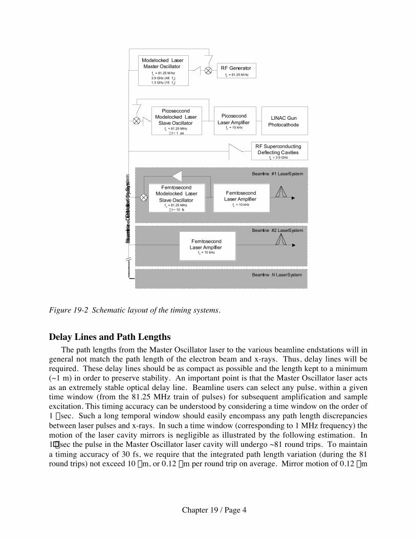
Chapter 19 / Page 4

RF SuperconductingDeflecting Cavities

fo = 3.9 GHz

PicoseccondModelocked Laser

Slave Oscillatorfo = 81.25 MHz

D t ~ 1 ps

PicosecondLaser Amplifier

fo = 10 kHz

FemtosecondModelocked Laser

Slave Oscillatorfo = 81.25 MHz

D t ~ 10 fs

FemtosecondLaser Amplifier

fo = 10 kHz

LINAC GunPhotocathode

FemtosecondLaser Amplifier

fo = 10 kHz

Bea

mlin

e D

istr

ibut

ion

Sys

tem

Beamline #2 Laser System

Beamline #1 Laser System

Beamline N Laser System

RF Generatorfo = 81.25 M Hz

Modelocked LaserMaster Oscillator

fo = 81.25 M Hz

3.9 GHz (48 fo)1.3 GHz (16 fo)

Figure 19-2 Schematic layout of the timing systems.

Delay Lines and Path LengthsThe path lengths from the Master Oscillator laser to the various beamline endstations will in

general not match the path length of the electron beam and x-rays. Thus, delay lines will berequired. These delay lines should be as compact as possible and the length kept to a minimum(~1 m) in order to preserve stability. An important point is that the Master Oscillator laser actsas an extremely stable optical delay line. Beamline users can select any pulse, within a giventime window (from the 81.25 MHz train of pulses) for subsequent amplification and sampleexcitation. This timing accuracy can be understood by considering a time window on the order of1 msec. Such a long temporal window should easily encompass any path length discrepanciesbetween laser pulses and x-rays. In such a time window (corresponding to 1 MHz frequency) themotion of the laser cavity mirrors is negligible as illustrated by the following estimation. In1!msec the pulse in the Master Oscillator laser cavity will undergo ~81 round trips. To maintaina timing accuracy of 30 fs, we require that the integrated path length variation (during the 81round trips) not exceed 10 mm, or 0.12 mm per round trip on average. Mirror motion of 0.12 mm

Chapter 19 / Page 5

within the 12.3 nsec round-trip time corresponds to a mirror velocity of 10 m/sec, which wouldrequire a force well beyond anything that could be generated from acoustic disturbances or fromthe piezoelectric transducer.

DEFLECTING CAVITIESOur scheme of manipulating the electrons followed by optical pulse compression carries the

advantage of providing insensitivity of the x-ray pulse timing at the sample following the crystaloptics, to the arrival time of the electron bunch in the deflecting cavities. An electron buncharriving "synchronously" with the deflecting RF voltage will experience a transverse kick ofequal amplitude and opposite direction to the head and tail electrons. Electrons in a buncharriving early or late with respect to the deflecting voltage zero phase will receive a similartransverse kick dependent on their position within the bunch, but the bunch also receives a netoffset kick and the centroid will oscillate afterward. Since the bunch duration is short comparedto the rf period (3.9 GHz deflecting cavities), the transverse kick to electrons within a bunchremains linear with the same slope. Figure 19-3 shows the perturbation to the electron bunch inthe deflecting cavities, resulting in time-position-angle correlation.

In the x-ray crystal optics, the optical path length varies linearly with transverse position onthe crystal, and early or late bunches produce radiation that will receive proportionately longer orshorter delays in the optical path, thus remaining synchronous with the deflecting cavity rf phase.Following the asymmetric crystal optics, the time of arrival of the x-ray pulses is the sameregardless of the jitter in arrival time of electron bunches at the deflecting cavity. In this way, thetemporal jitter of the electron beam is transformed into spatial jitter of the x-ray pulse. Figure.19-3 gives a pictorial view of this scheme.

Chapter 19 / Page 6

Figure 19-3 The hard x-ray production scheme, showing the electron bunch in the deflecting rffield with different arrival times with respect to the cavity phase. Bunches arrivingearly or late in the cavity still experience a distribution of particles in alignmentwith those of a bunch arriving in phase with the cavity field. X-rays from suchbunches experience the same compression in the x-ray optics, resulting in improvedtiming stability, but with a geometric translation of the x-ray pulse on the sample.

Low-level rf system for the superconducting deflecting cavitiesAs described above, with the deflecting cavity locked to the laser oscillator, stability of the x-

ray pulse will depend on the phase stability of the deflecting cavity voltage. The low-level rfsystem for the superconducting deflecting cavities is instrumental in determining the finalsynchronization between the beamline lasers and the femtosecond hard x-rays. The rf drivesignal at 3.9 GHz is derived directly from the Master Oscillator via illumination of a photodiodeand subsequent electronic amplification. Since the fundamental rf signal at its source isabsolutely locked to the laser pulses from the Master Oscillator, maintaining this synchronizationis largely an issue of feedback control of phase while minimizing the electronic noise from the rfamplifiers and isolating (or actively damping) the deflecting cavities from external acousticperturbations.

Compressed x-ray pulse

Synchronous bunch

Early bunch

Late bunch

Asymmetrically cut crystal

Dt Dt

electron bunch

laser pulse

x-rays

LASER OSCILLATOR(passively modelocked)

3.9 GHz(RF Kick)

Chapter 19 / Page 7

A 10 fs timing error is equivalent to 0.014° in phase at 3.9 GHz, and we require control atthis level. Resolution of 1 fs requires measurement to 2.44x10-5 rad, or one part in 41,000. A 16-bit DAC offers the required resolution. The system bandwidth of approximately 100 Hz allowsample time for signal processing.

The superconducting cavity has an external bandwidth requirement of approximately 100 Hzto allow feedback control of phase and amplitude required due to cavity resonant frequencyperturbations arising from microphonically induced changes in cavity geometry.

A photodiode or similar optical-electrical transducer illuminated by the Master Oscillatorsignal can be attached to an electrical band-pass filter at 3.9 GHz, to provide a stable drivesignal. At least one isolation stage is needed, either low noise active or a circulator, before thissignal is used for measurement and control of cavity fields. Figure 19-4 shows a schematic of thedeflecting cavity rf system electronics.

Designing for low jitter really means designing for low noise. Over time spans of 10-100 ms(100 to 1000 pulses), temperature changes and 1/f effects become important, and timing errorbetween the x-ray pulse and the experimental excitation pulse, measured at a beamline endstationwill provide a (digital) correction signal for cavity phase over this time period. The cavity controlsystem only has to keep the accelerator stable long enough to get good signal/noise out of thepump laser/x-ray pulse relative timing measurements, and for those results to propagate throughnetworks and software filters to update the digital setpoints.

Numerology of the timing frequencies is important. A simple integer scaling from theMaster Oscillator to RF frequencies is probably bad, as that places the output of the mixers atDC. Quarter integer scaling places the output frequency at about 20 MHz for both the 1.3 and3.9 GHz cavities, which would provide traditional I/Q/-I/-Q output from an 80 MSample/s ADC.Figure 19-2 shows the deflecting cavity rf system schematic diagram.

Although 16-bit 80 MSample/s ADCs do not exist at the time of writing, currently availableparts (AD6645, 14-bit, 75 dB SNR at 15 MHz and 80 MSample/s) come close enough to allowmeaningful tests and future developments may be expected to provide for our requirements.

Chapter 19 / Page 8

Figure 19-4 RF systems control schematic for the deflecting cavities.

We estimate the thermal noise in the system by assuming a room temperature (T) amplifierwith 3 dB noise figure (NF) and 30 dB gain (G), bandwidth (∆f) 100 Hz. The noise power

(1)is then 8x10-16 W or 2x10-7 volts in 50 Ω (k is the Boltzmann constant). A 7 dB NF mixer wouldcontribute significantly less noise. A resolution of 1 fs requires that the signal equivalent to a 1 fsphase change be greater than the noise level, and we find that the cavity signal amplitude must begreater than approximately 10 mV. Such a signal level may readily be obtained from a cavityprobe. A similar analysis shows that thermal noise in the photodiode and rf drive chain is notexpected to prove problematic.

Low-level rf system for the photocathode rf gunSince the bunch compression scheme transforms energy jitter from the injector into timing

jitter in the main linac, the launch phase of the electron bunches must be controlled to stabilizeenergy jitter to an acceptable level. While the rf signal derived from the Master Oscillator isexpected to be stable to ~100 fs, a low-level rf system similar to that shown in Figure 19-4 maybe applied to control the launch phase of the photocathode gun rf fields with respect to thephotocathode laser pulse.

Pthermal= k T D fNF G

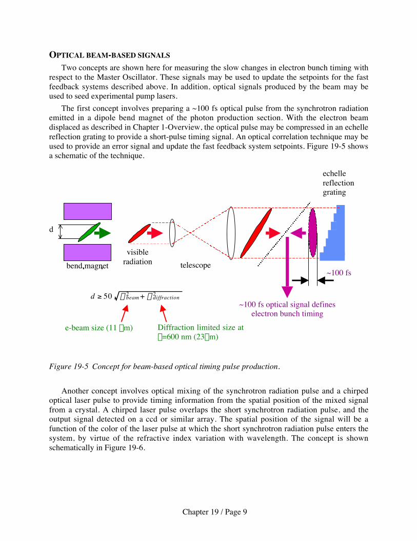
Chapter 19 / Page 9

OPTICAL BEAM-BASED SIGNALSTwo concepts are shown here for measuring the slow changes in electron bunch timing with

respect to the Master Oscillator. These signals may be used to update the setpoints for the fastfeedback systems described above. In addition, optical signals produced by the beam may beused to seed experimental pump lasers.

The first concept involves preparing a ~100 fs optical pulse from the synchrotron radiationemitted in a dipole bend magnet of the photon production section. With the electron beamdisplaced as described in Chapter 1-Overview, the optical pulse may be compressed in an echellereflection grating to provide a short-pulse timing signal. An optical correlation technique may beused to provide an error signal and update the fast feedback system setpoints. Figure 19-5 showsa schematic of the technique.

Figure 19-5 Concept for beam-based optical timing pulse production.

Another concept involves optical mixing of the synchrotron radiation pulse and a chirpedoptical laser pulse to provide timing information from the spatial position of the mixed signalfrom a crystal. A chirped laser pulse overlaps the short synchrotron radiation pulse, and theoutput signal detected on a ccd or similar array. The spatial position of the signal will be afunction of the color of the laser pulse at which the short synchrotron radiation pulse enters thesystem, by virtue of the refractive index variation with wavelength. The concept is shownschematically in Figure 19-6.

e-beam size (11 mm) Diffraction limited size atl=600 nm (23mm)

d

bendmagnet

visibleradiation

-

~100 fs

echellereflectiongrating

~100 fs optical signal defineselectron bunch timing

bend magnet telescope

d ≥ 50 s beam2 + s diffraction2

Chapter 19 / Page 10

Figure 19-6 Concept for beam-based optical timing pulse production.

REFERENCES[1] D. E. Spence, J. M. Dudley, K. Lamb, W. E. Sleat, and W. Sibbett, “Nearly quantum-limited

timing jitter in a self mode-locked Ti:sapphire laser,” Opt. Lett., 19, 481-483, 1994.[2] R. K. Shelton, S. M. Foreman, L. S. Ma, J. L. Hall, H. C. Kapteyn, M. M. Murnane, M.

Notcutt, and J. Ye, “Subfemtosecond timing jitter between two independent, activelysynchronized, mode-locked lasers,” Opt. Lett., 27, 312-314, 2002.

[3] J. Son, J. V. Rudd, and J. F. Whitaker, “Noise characterization of a self-mode-lockedTi:sapphire laser,” Opt. Lett., 17, 733-735, 1992.

[4] C. X. Yu, S. Namiki, and H. A. Haus, “Noise of the stretched pulse fiber laser: Part II -experiments,” IEEE J. Quantum Electron., 33, 660-668, 1997.

[5] S. Namiki, C. X. Yu, and H. A. Haus, “Observation of nearly quantum-limited timing jitter inan all-fiber ring laser,” J. Opt. Soc. Am. B, 13, 2817-2823, 1996.

[6] J. Ranka, R. Windeler, and A. Stentz, “Optical properties of high-delta air-silicamicrostructure optical fibers,” Opt. Lett., 25, 796-798, 2000.

e-beam size(11 mm)

diffraction size at l=600nm (23mm)

bend magnet

visibleradiation

-

~100 fs

echellereflectiongrating

Non-linear crystalChirped laser pulse

CCDBend magnet visible SR

Chapter 20 / Page 1

20. BEAM DUMP

A beam dump for the continuous absorption of the electron beam will be located downstreamof the photon production arc. It is anticipated that the beam dump assembly will include anupstream bend magnet that directs the electrons towards a water-cooled dump located belowfloor level. A series of two beam windows, located between the dump and bend magnet, isolateand safeguard the beamline from contamination by the gas evolved from the dump. A partialpressure of argon gas between the windows will be monitored as a means of detecting a vacuumbreech. Additional magnets to raster the beam upstream of the windows may be required toprevent excessive localized heating.

As with the other mechanical systems, the beam dump was designed to be compatible withthe upgraded machine parameters of 3.1 GeV and 3 nC charge per bunch on a 10 kHz repetitionrate (93 kW of beam power). The successful design a high power multi-GeV beam dump musttake into consideration several factors including:

• cooling requirements• thermal stresses• safety – minimal reliance on active components• radiation shielding• activation and handling of activated components• hydrogen generation (water cooled dumps) and handling• fabrication feasibility and cost• operating costThis initial study primarily addresses thermal issues with some regard for fabrication

feasibility. Estimates of the required shielding, hydrogen generation and safety issues are inprogress.

The initial dump design, Figure 20-1, consists of a solid 24 cm diameter central cylinder ofPOCO graphite surrounded by a 2 cm thick copper outer layer. The copper is brazed to thegraphite to produce a good thermal bond. The carbon/copper assembly resides within a waterjacket. The 2-meter length of the carbon center plug is sufficient to absorb most of the energy ofthe electromagnetic shower. A 5 cm thick OFHC copper end plug will absorb the low energytail. The combined radial thickness of copper and carbon is sufficient to absorb more than 99%of the energy in the transverse direction. Water flowing at a modest rate over the surface of thecopper removes 93 kW of heat on a steady-state basis.

carbon

Chapter 20 / Page 2

Carbon has the advantage of a relatively long (physical) radiation length and excellentthermal conductivity. Pure aluminum has roughly twice the thermal conductivity but less thanhalf of the radiation length of carbon whereas copper has about 4 times the conductivity but lessthan 1/10 the radiation length. A long physical radiation length leads to a broad longitudinalelectromagnetic shower profile and an enhanced radial power deposition. Diffuse longitudinalenergy absorption spreads the heat over a greater effective surface area for cooling (at theperimeter) and reduces the peak temperatures. High thermal conductivity allows for a greaterradial path length from heated core to cooled surface (for a given peak temperature) and thus alower power density at the convection boundary due to increase in outer surface area with radius.

A comparison of the power deposition for three candidate absorber materials is shown inFigure 20-2. Power deposition profiles were determined using the formulas for electromagneticcascades in European Physical Journal C, Particles and Fields [1].

Figure 20-1 Beam absorbing assembly.

Copper

Water Passage

Manifold

Graphite

Chapter 20 / Page 3

0

1000

2000

3000

4000

5000

6000

7000

8000

0 50 100 150 200 250 300

Depth (cm)

Po

wer

Dep

osi

tio

n (

W/c

m)

carbon

aluminum

copper

Figure 20-2 Power deposition profiles of an electromagnetic cascade in carbon, aluminum andcopper for a 3.1GeV, 93kW electron beam.

The transverse development of electromagnetic cascades scales with the Moliere radius, RMgiven by [1]

CS0M E/EXR = (1)

where ES = 21.2 MeV, Z = atomic weight, Xo is the radiation length, and

24.1Z

MeV610EC +

= (2)

The critical energy, EC, is the energy at which the ionization loss per radiation length is equalto the electron energy [2]. Approximately 90% of the energy is contained within one RM and99% is contained within 3.5 RM. For copper RM = 1.5 cm and for carbon RM = 4.8 cm. Toapproximate the transverse power deposition, a single Gaussian distribution with s = RM / 1.65(90% of the swept volume is contained within a radius of RM). Setting the area under thetransverse profile equal to the power dissipation at a given depth of absorber gives thevolumetric power deposition at any point in the absorber volume. The actual distribution startsas a narrow core and broadens as the cascade develops so the assumed constant transverse profileunderestimates the volumetric power density over the initial length of absorber. Furtherrefinement in this area is required to determine if the electron beam must be rastered.

Chapter 20 / Page 4

The calculated absorbed power density in carbon peaks at roughly 5 W/cm3 and falls offradially to less than 0.5 W/cm3 at a radius of 16 cm. To estimate the temperature rise andthermal stress the power density was applied to an axisymmetric FEA model (ANSYS). Theresultant temperature and stress plots are shown in Figures 20-3 and 20-4.

Figure 20-3 Temperature profile for carbon/copper beam dump over the first 75 cm. Convectiveheat transfer coefficient of 2000 W/m2-C applied to outer surface.

The model encompasses the first 75 cm of absorber length, corresponding depth of theenergy deposition peak. A symmetry boundary condition was applied at the x = 75 cm end totake advantage of the near symmetry in the longitudinal energy deposition profile.

The convective heat transfer coefficient of 2000 W/m2C is consistent with 25 oC waterflowing over the surface at 0.37 m/s. This can be achieved by passing water at 2 l/s through aconcentric passage having an annular gap of 6 mm. Note that the calculated peak temperature ofthe graphite is very modest and that the temperature at the convective boundary (in contact withwater) is well below boiling.

OFHC Copper,2cm thick

POCO Graphite,12cm radius

Temperature contoursin Centigrade,

Water temp = 25 C

Chapter 20 / Page 5

Figure 20-4 Stress contours (von Mises equivalent) for a carbon/copper beam dump, first 75 cm.

The structural boundary conditions mirror the thermal case with a symmetry boundaryapplied at x = 75 cm. The thermal stresses are very modest in comparison to the tensile strengthof POCO graphite of 3500 – 7000 N/cm2 (5000-10000 psi) and the yield strength of annealedOFHC copper of 7000 N/cm2 (0.2% offset).

On the basis of this initial study, the ability to construct a beam dump capable ofwithstanding the power of the proposed re-circulating linac running at an upgraded energy andelevated bunch charge (3.1GeV, 3 nC) appears feasible. Peak temperatures and thermal stressesare relatively low for a reasonably sized water-cooled absorber constructed from carbon andcopper. The design of the upstream windows and power dissipation at shower incipience mayrequire that the beam be rastered. Radiation shielding, activation and cost issues are yet to beaddressed.

REFERENCES: [1] European Physical Journal C, Particle and Fields Vol. 15, pp.167-171, Nov 1, 2000.

Stress contours inN/cm2

Peak stress in copper< 20% of yield strength

Chapter 21 / Page 1

21. CONVENTIONAL FACILITIES

Architectural DesignThe preferred site of the proposed femtosecond x-ray facility is in the Old Town area of

Berkeley Lab in close proximity to the Advanced Light Source (ALS). The conventionalfacilities will consist of a two story building of approximately 125,000 gross square feet, and twoseparate free standing structures – a Cryogenic Plant, that will provide liquid helium for coolingof the accelerator, and an Utility Center, that will house heavy equipment for mechanical andelectrical building systems support.

The high bay first floor of approximately 91,000 gross square feet will house the machineconsisting of injector, linear accelerator, magnetic arcs, and production beam array of undulatorsand bend magnets, producing multiple beamlines. In addition to the machine, the first floor willprovide experimental area, assembly areas, and laser rooms. There will be a continuouscirculation pathway along the perimeter of the building to facilitate emergency exiting and day-to-day circulation between the functional areas. The structural bay housing the acceleratormachine will be equipped with a 10-ton crane to facilitate installation and maintenance of theaccelerator components. The experimental area will be served a by a monorail following theoutline of experimental stations.

The second floor will house the control room, and a mixture of user labs consisting of wetlaboratories, dry laboratories, and semi-clean rooms. Adjacent to laboratory areas will be offices,conference rooms, and a core of support facilities including cold rooms, dark rooms, equipmentrooms, and similar research support spaces. Because of the extremely tight footprint, themechanical and electrical equipment room will be also located on this level. Great care will betaken to isolate the electrical a mechanical equipment to minimize the vibration and acousticalimpact. The structural design will provide for future expansion of the second floor.

The building design is taking advantage of the sloped topography of the site. The buildingwill be accessible from Segre road and from an upper roadway circling the existing historicallysignificant grove of redwood and pine trees. The main lobby, entered from the upper road, willbe located on a mid-level with an elevator and stair connection to both first and second floors. Asmall lobby with a stair and an elevator will be provided on the opposite side of the buildingaccessed from Segre Road and adjacent to truck access for staging of scientific equipment.

The exterior finish of low maintenance, factory preformed and painted, metal siding andclear glass with low emissivity coating will be compatible and complementary to the ALScomplex. The roof will be a single sheet roofing membrane system with heat reflective coatingto reduce solar gain. Metallic screens will conceal rooftop mounted mechanical exhaustequipment. An enclosed pedestrian bridge will link the building with ALS to facilitate cross-disciplinary collaboration of users in both facilities.

The femtosecond x-ray source project will make every effort to deliver an environmentallyresponsible design, construction, and operation. Its environmental impact will be reducedthrough sensitive site development; control of southern and western solar loads by means ofblinds, sunshades, and recessed windows; water and energy conservation; and environmentallyresponsible building materials.

Chapter 21 / Page 2

The building will be protected by a sprinkler system connected to the LBNL fire alarmsystem. Smoke detection and other detection systems will be provided where required. Thebuilding will be designed in conformance with requirements for group ‘B’ occupancy as definedby the California Building Code (CBC), Type II fire resistive construction, and seismic safetyand fire safety code requirements. The building will comply with disabled accessibilityrequirements in accordance with the Americans with Disabilities Act (ADA).

The project is sited in conformance with the LBNL Site Development Plan. The project siteis currently occupied by several old buildings used by the ALS, Accelerator and Fusion ResearchDivision (AFRD), Engineering, EH&S, Earth Sciences Division (ESD), and Facilities forresearch and other activities. These activities will be relocated.

Structural DesignStructural design shall account for all loads to which earth retaining systems and the building

structure may be subjected including static, live, wind, seismic, etc. The design will comply withthe requirements of the California Building Code (CBC) and LBNL’s Lateral Force DesignCriteria.

The first story of the building will be cast-in-place reinforced concrete slab-on-grade withtied back reinforced concrete retaining walls on the east, northeast and southeast sides. The westbay of the first story will contain cast-in-place concrete shielding structures at the beamlinebends and be serviced by a top riding ten (10) ton crane. The upper floor and roof will beconcrete slabs on metal deck supported by structural steel floor joists spanning betweenstructural steel jack trusses supported by long span structural steel trusses and steel columns. Inthe transverse direction, the building will be a moment resisting frame and, in the longitudinaldirection, various structural framing systems, such as eccentrically braced frames, concentricallybraced frames and moment resisting frames, will be compared in the Title I design stage todetermine the most suitable and cost effective system. The foundation system of the westernportion of the building, including the shielding structures, will be drilled piers with reinforcedconcrete pier caps interconnected by tie beams. The foundation system of the eastern portion ofthe building will be isolated footings founded on bedrock and interconnected by tie beams.

Roofs shall be designed for a minimum mechanical equipment load of 50 lb/sq ft or theactual weight of the mechanical equipment, whichever is greater. The elevated floor will bedesigned for a 125 psf live load.

Nonstructural building elements and the mechanical and electrical systems will be designedto accommodate calculated displacements due to lateral forces from wind or seismic forces.

Mechanical DesignHeating, Ventilation and Air Conditioning System

The experimental floor and the second floor laboratories and offices will be heated or cooledwith tempered air to maintain inside design temperatures 76°F ± 2o F in summer and 72°F ± 2o Fin winter. Precise temperature control at 25°C ± 0.5°C (77°F ± 0.9°F) will be maintained in

Chapter 21 / Page 3

shielding tunnels and laser rooms. Humidity control is not expected to be required. Theminimum ventilation rate will be 1 cfm/ft2.

Air supply air handling units (AHU) will be housed in the second floor mechanical room.Exhaust fans will be mounted on the roof of the building within a screened area. The chillersand boilers will be located in the Utility Center. Chilled and heating hot water will be pipedfrom the Utility Center to the AHU to provide pre-cooling and pre-heating. Final buildingheating will be provided by individual re-heat VAV boxes located throughout the building. Eachunit will be provided with a dedicated temperature sensor to control re-heating and airflow fromeach individual VAV unit.Process Piping

Mechanical utilities will include domestic cold and hot water (DC/HW), industrial cold andhot water (IC/HW), chilled water (CWS/R), low conductivity water (LCWS/R), compressed air(CA), vacuum (VA), fire sprinkler supply (FSS), sanitary sewer (SS), and helium (He) forcryogenic plant. The utilities on the main floor will be run in the trenches recessed in theconcrete floor and terminate at valve stations at fixed locations compatible with acceleratorassemblies or locations compatible with user needs. Liquid nitrogen will be provided by thecryogenic plant and will be piped or distributed in dewers to experimental stations andlaboratories. Deionized water will be distributed through the second floor laboratories andpolishing stations will be provided at points of use.

The following underground piping systems will require modifications and additions due toconstruction: low-conductivity water supply (LCWS), low-conductivity water return (LCWR),compressed air (CA), fire sprinkler supply (FSS), Sanitary sewer (SS), storm drain (SD), high-pressure city water (HPCW), high-pressure natural gas (HPNG), treated water supply (TRWS),treated water return (TRWR). Temporary mechanical and underground utility services will beprovided to all adjacent buildings and operations that will be affected by the construction work.Energy Conservation

A dynamic computer analysis technique will be used to evaluate energy conservationalternatives and life cycle costs, determine design energy consumption, and determine passiveand active solar effects. Use of renewable energy systems will be evaluated and utilized whenshown to be cost effective. The heating and ventilating systems will be controlled by the JohnsonControls, Metasys digital control system. The control system will have central monitoring.Control strategies will include temperature control, VFD-controlled fans, chillers, cooling towerfans, pumps, night set back (with override), economizer, and other applicable energyconservation strategies.

Electrical DesignPower requirements for the building are projected at approximately 10 MGW, with

2-3 MGW for cryogenic plant, 3 MGW for the accelerator and ~4 MGW for user load. Thebuilding will be served by a dedicated electrical substation located on a separate pad in thevicinity of the Utility Center. The building will be served by 480/277 V and 208/120 Vdistribution systems with panelboards, branch circuit panels and step-down transformers locatedin dedicated electrical room.

Chapter 21 / Page 4

An emergency generator will be located in the Utility Center. Emergency power loads willinclude emergency egress lighting, fume hood and helium exhaust, and back up for compressorsand other research equipment. UPS will provide power for sensitive computer and controlequipment through emergency generator start-up time.

Lighting controls will be zoned, automated, and integrated with the Energy Management andControl System. Enclosed offices will be individually switched and controlled with occupancysensors. Where natural light is available, two-level switching or photocell controls will beutilized. Task and specialty lighting will be provided where required.

Emergency lighting will be provided in laboratories, corridors, stairwells and other publicareas by connecting selected fixtures of the general lighting system to standby power circuits.Building exit signs and emergency egress lighting units will be provided with 90-minute backupbattery packs and be connected to the standby power system.

The building will be equipped with telephone, communications, fiber-optic data circuits,paging and public address system, and building entry security system.

A complete building fire alarm system with extensions to the to the existing hill-wide LBNLfire alarm system will be provided.

Gross Area SummaryBuilding

First Floor 91,000 SFSecond Floor 34,000 SF

Separate Structures:Cryogenic Plant 10,000 SFUtility Center 4,000 SFSwitching Station 3,600 SF

First Floor (Gross SF)Experimental Area 16,000 SFAssembly Area 7,000 SFLaser Rooms (2 @ 250 SF) 500 SFMachine 53,500 SFLobby and Circulation 14,000 SF

Second Floor (Net SF)Laboratories, Research Support 12,000 SFOffices, Conference RoomsLounge, Lobby, etc. 8,500 SFControl Room 500 SFMechanical/Electrical Room 4,000 SF

Chapter 22 / Page 1

22. SITE SELECTION

SITING ASSESSMENTA two-step siting assessment process was undertaken in considering locations for the

proposed facility. The first step of the siting process was initiated concurrent with discussionsamong the scientific personnel aimed at determining operational and research associationsbetween the proposed building and other research activities at the Laboratory. In the initial orfirst pass assessment, sites that might physically accommodate this new building were identified.Possible sites were identified on the main Laboratory site, on lands immediately to the east of theLaboratory site, and in the neighboring cities of Richmond and Alameda (sites within a 15-mileradius of the Laboratory). Each of these sites was then evaluated as to their ability toaccommodate the facility. All but four of the first-step sites were eliminated. Most wereeliminated as essential utilities were not available in the general area or because the localjurisdiction had already made other plans for the site, and a number of the sites were eliminatedas upon closer review they could not accommodate a building of the required size. The sitesidentified and considered in this phase are illustrated in Figure 22-1.

Four sites advanced for further consideration in the second phase; two on the Laboratory siteand two at the University of California’s Richmond Field Station. Each of the four sites werefound to be feasible during this second phase review, however, in the end not all sites wereranked equally. One site, the Building 51 site, was not the top recommended site as a largeformer accelerator building remains on this site and this large structure is not scheduled to bedemolished in a timeframe consistent with that preferred for the ultrafast dynamics facility. Itwas determined that acceleration of the demolition process would add approximately $40M tothe cost of this project. The two sites in the City of Richmond are not the top recommended siteas the research community determined that there are both scientific and operational benefitswhich would be lost in selecting a site approximately 15-30 minutes travel time from theLaboratory site. Moreover, it was determined that these sites would also require speciallyengineered foundations to ensure proper stability of the beam line floor. These two sites areadjacent to liquefaction zones and are on a sandy loam that carries vibration waves from adjacentrailroad and industrial operations.

Chapter 22 / Page 2

Figure 22-1 First pass sitting options

Highest Ranked SiteThe highest ranked site for the proposed facility is immediately to the east of the Advanced

Light Source (ALS). This site is in the Old Town area of Berkeley Lab (see Figure 22-2 below)and is currently occupied by a number of small buildings. The four primary factors driving thisrecommendation are summarized below:

Scientific and operational relationships with the ALS. Both the ALS and the proposedfemtosecond dynamics facility are x-ray light sources dedicated to user experiments. The ALSand the femtosecond dynamics facility provide opportunities to conduct different butsynergistically related research. An enclosed pedestrian bridge could link the femtoseconddynamics facility building with the ALS and facilitate both cross-disciplinary collaboration ofusers and efficient staffing of both facilities. Provision may be made for possible future beamlineand end-station integration between the two facilities.

Utility Infrastructure. The proposed site is adjacent to a recently upgraded electricalsubstation with capacity to meet the needs of this facility as well as other future growthrequirements of the Laboratory. The Laboratory obtains federal power via this substation.

Chapter 22 / Page 3

Stable Geology. The proposed site requires little excavation to reach stable bedrock. Thissite provides superior building stability, an important factor as beamline stability and alignmentare paramount issues in the operation of this facility.

Site Renewal. The proposed Old Town site currently contains a number of small anddifficult to effectively utilize W.W. II-era buildings. These buildings have provided over 50-years of scientific service but no longer meet modern building codes or scientific researchstandards. Moreover, these buildings can not be cost-effectively upgraded to serve modernscience and in general they are expensive to maintain in even a minimal operating condition.Thus siting at this location removes structures that are operational liabilities and replaces themwith facilities fully capable of supporting the next generation of scientific research.

At this site, the building design can take advantage of a gently sloped topography.Excavation costs will be moderate. Moreover, there are design benefits as well. The experimentalfloor of the proposed building would be directly accessible from the adjacent road (Segre Road),while the upper floor offices and laboratories would be made directly accessible from anotherroad (Road “R”). The main entrance to the upper level will be from a parking lot adjacent to asignificant grove of redwood trees. The main lobby, entered from the upper road, will be locatedon a mid-level with an elevator and stair connection to both first and second floors.

The project is sited in conformance with Berkeley Lab’s Long-Range Development Plan(LRDP); this LRDP foresaw and supports redevelopment of this site.

The Laboratory Site Remediation office conducted a review of sub-surface contaminationrecords in the project area. This study concluded that scientific buildings such as those proposedare fully permissible at this location. It was also determined that standard precautions would berequired for the identified contaminants. In general, the contamination is low-level and isgenerally a considerable distance below the proposed foundation elevation of the new building.A small-contaminated groundwater plume to the east (which is already being managed) can becontrolled using standard technologies. Small and localized areas of soil contamination may existunder the foundations of some of the still standing buildings, we recommend a sampling programfor these areas prior to excavation and removal of soil. The report also notes that an updated risk-assessment may be required if the design of the building varies considerably from theassumptions that are at the basis of the current risk assessment.

Chapter 22 / Page 4

Figure 22-2 Top ranked location for a femtosecond dynamics facility at Berkeley Lab. TheAdvanced Light Source is the round building (6) immediately to the left of thisfemtosecond dynamics facility site.

Groundwater ContaminationThe proposed accelerator site (Old Town or OT site) lies above a broad multi-lobed plume of

groundwater contamination known as the Old Town Plume. Contaminants detected ingroundwater are primarily halogenated non-aromatic volatile organic compounds(VOCs)(primarily industrial solvents [perchloroethene aka tetrachloroethene [PCE], trichloroethane[TCA], carbon tetrachloride], solvent degradation products [dichloroethene [DCE],dichloroethane [DCA], vinyl chloride, chloroform, etc], or both [trichloroethene [TCE]]). andlesser quantities of fuel hydrocarbons (diesel/kerosene and crude/waste oil).

Groundwater flow directions and maximum recorded groundwater elevations in the vicinityof the OT site have been determined; groundwater flow is northwestwards in the northern part,and southwestwards in the southern part of the site. The depth to groundwater variesconsiderably due to the differing hydraulic properties of the rocks beneath different parts of thesite. The lobes of the Old Town Plume comprise several subplumes derived from multiplesources, which, primarily as a result of groundwater movement, have commingled to form thelarger area of groundwater contamination. As a result, contaminated groundwater generallycontaining tens to hundreds of µg/L (commonly referred to as parts-per-billion [ppb]) underliesmost of the OT site. Following is a description of each lobe of the plume.• The Building 7 lobe of the Old Town Plume contains the highest levels of contamination and

has a principal contaminant source (the Building 7 sump) north of Building 7. This lobe lies

Femtosecond Structural DynamicsUser Facility

Chapter 22 / Page 5

entirely downgradient from the OT site (i.e. flow within the plume is away from the site), sois largely irrelevant to site development plans.

• The Building 52 lobe has substantially lower contaminant concentrations than the Building 7lobe, but immediately underlies the northern part of the OT site. However, groundwater liesat a significantly greater depth than the expected foundation depth for the proposedaccelerator, so no direct foundation to groundwater contact would occur.

• The Building 25A lobe also has relatively low contaminant concentrations compared to theBuilding 7 lobe. However, flow within this lobe is westward towards the center of the OTsite, and recently a groundwater collection trench has been installed south of Building 44 tolimit further westward migration of contaminated water. Analysis based on information fromwells in the area shows that the groundwater highstand elevation (i.e. the highest recordedgroundwater elevation) in this lobe intersects the OT site building footprint, indicating thepotential for groundwater seepage into the excavation and contact between the buildingfoundation and contaminated groundwater. However, it should be noted that the groundwaterelevation as measured reflects the rise of groundwater into wells that have screens locatedbelow the elevation of the proposed building foundation, and, given the low permeability ofrocks in this area, does not indicate that groundwater would in fact flow into the buildingfoundation excavation. Insufficient data are currently available to evaluate whether or notgroundwater seepage would occur into the excavation.

Development of the OT site would need to include mitigation of the following groundwatercontamination impacts:• Protection of construction workers from potential direct groundwater exposure while

excavating the eastern portion of the foundation• Capture, treatment and disposal of contaminated groundwater (if encountered) both during

construction and after completion of the building• Assessment and mitigation of toxic vapors that might migrate from groundwater through the

soil into overlying buildings or into the excavation.Generally, protection of construction workers would be assured through preparation of a

construction risk management plan that included site monitoring and contingency plans. Ifgroundwater was encountered during construction, capture and treatment would likely involveinstallation of extraction wells, sumps, or trenches, and construction of a temporary treatmentsystem. It is likely that building subdrains (if needed) would need to be constructed asremediation systems to capture all groundwater that could potentially contact buildingfoundations, and discharge it to a groundwater treatment system. The rainwater collection systemfor the building would need to be constructed so as to ensure that rainwater effluent was notmixed with groundwater in the subdrain system. A similar mitigation measure is currentlyemployed at Building 46, where the previously existing subdrain has been adapted to capture thedowngradient edge of the Building 52 lobe.

Chapter 22 / Page 6

Human Health AssessmentA human health risk assessment is currently in progress as part of Berkeley Lab’s RCRA

Corrective Measures Study. Preliminary results indicate that risks to building occupants at theOT site from vapor migration are generally below thresholds of concern (e.g. incremental risksless than 10-6) except for a very small area at the north end of the site. However, these results arebased on the assumption of buildings located at the current ground surface and groundwatercontamination remains at the present level. Since the Old Town site would apparently involve anunusually large excavation, the depths to groundwater beneath the building would decreasesubstantially from those utilized in the risk assessment, thus increasing risks. On the other hand,the recently completed Building 25 Corrective Measure may lower the level of contamination ingroundwater over the next few years. Therefore, it would be necessary to reevaluate risks basedon the proposed building design and the future groundwater contamination level, probablythrough a combination of modeling and vapor sampling. In the event that risks were shown to besignificant, it is likely that regulatory agencies would require building construction modifications(e.g. vapor barriers beneath foundations, and possibly a continued monitoring plan) to mitigatepotential risks.

Soil ContaminationSoil contamination associated with a number of historic sources exists within the proposed

accelerator site. These include:• PCBs and petroleum hydrocarbons at Area of Concern (AOC) 10-2, the former Building 52

hazardous materials storage area. Low levels of these contaminants are present in shallowsoil (primarily <5 feet) in areas immediately adjacent to Building 52.

• PCBs, petroleum hydrocarbons and some metals at Solid Waste Management Unit (SWMU)10-4, the Building 16 Former Waste Accumulation Area. Low levels of these contaminantswere present in shallow soil on the slope west of Building 16.Other soil contaminants are present at scattered locations at the OT site, but at levels less

than regulatory cleanup standards for the site, and would not be triggers for construction or officeworker protection measures. However, waste management regulations would effect disposal ofsuch soils as wastes. Therefore, a soil management plan would need to be developed thatincluding provisions for sampling, analysis, waste profiling, transportation and disposal of wastesoil.

Given the long history of multiple uses of the OT site, it would be prudent to conductsampling of currently inaccessible soil beneath buildings as they were demolished, with analysesconducted based on historical building use patterns. Proposed sampling scope and procedurescould be included in the soil management plan discussed above.

Chapter 23 / Page 1

23. TECHNICAL RISK ANALYSIS

IDENTIFICATION, ASSESSMENT, AND MITIGATION OF TECHNICAL RISKSKey objectives of this feasibility study are:

1. Identify all of the technology challenges2. Define the R&D needed to ensure that all critical components have an acceptable risk

by the start of the final/detailed design phase

The major systems and components have been reviewed and the associatedtechnology, design and engineering, and manufacturing risks assessed. The criteria foridentifying and assessing these technical risks are discussed below. The assessment ofthe technical risks is based on in-house expertise and information from key members ofthe accelerator technology community.

Our goal for the R&D program is that all critical technologies reach the followingTechnology Maturity Levels (TML) by specific phases of the project development:

• TML Low to Medium by CD0, identification of mission need and beginning ofconceptual design phase

• TML Medium to High by CD1, approved baseline and start of the detailed designphase

• TML High by start of the fabrication phase

Reaching these levels of technology maturity means reduced development risk, whichtranslates into lower cost, schedule, and performance risks. Table 23-1 summarizes theresults of the risk identification and qualitative assessment to-date and does not reflect theimplementation of the risk reduction plans discussed later. Risk analysis will be ongoingthroughout the project to monitor the status and progress of the risk reduction effort.

Chapter 23 / Page 2

Table 23-1 Summary of the technical risk assessment

Item Risk Factors1 Comments3

R&D 2 D&E2 Man.2RF photocathodegun

M H M Warm copper RF photocathode gun demonstrated for lowoperation rate. D&E effort to operate reliably at high rate.

Photocathode M M M Recent results indicate good lifetime for Cs2Te at highvacuum.

Photocathode laser M M L Laser pulse needs high temporal and amplitude stability.Flat beam M L L Uses demonstrated technique with standard optics.SC linacs M M M Uses SoA SC RF cavities based on TESLA TTF; some

different parameters; much higher cryogenics loads.Beam spreadersection

L M L Uses some specialized magnets based on experience. Tightgeometry poses D&E challenge.

HGHG FELs M M M Successful proof-of-principle experiment in IR regionpromising for the generation of higher energy photons.

Deflecting cavities H H/M M Uses SoA SC RF cavities. Stringent requirements forstability, HOM and LOM damping.

Lattice magnets L L L Uses standard water-cooled electromagnets.Undulators M H/M H/M Trade between permanent and SC undulators is still open:

performance vs. risks. May use several different undulators.Beamline optics M M L SoA optics with some different parameters for pulse

compression.Beam dump L L L Similar to existing beam dumps.Diagnostics andinstrumentation

L M L Use of demonstrated techniques with some newrequirements for measurement of beam tilt.

Synchronization H H M Tight requirements for x-ray pulses, electron bunches, andpump lasers.

Pump lasers M M L Tight synchronization required with deflecting cavities.Control systems L M L Faster acquisition rates than ALS. Important to efficient

commissioning and operations.Low-level RFsystems

M M L Adjustable tuners save power. Some development requiredusing standard techniques.

Vacuum systems L L L Similar to existing designs.

Notes:1. The risk assessment reflects the present status of major components2. R&D: Research and Development, D&E: Design & Engineering, Man: Manufacturing

The criteria for the assigned risk factors are:H (HIGH): Concepts and/or prototypes need to be developed.M (MEDIUM): Similar components or subsystems have been successfully demonstrated or requiresome extrapolations from existing designs.L (LOW): Subsystems and components are essentially identical to existing and proven designs.

3. Details are presented in the text.

Specific risk mitigation plans are being developed and implemented for all the high-and medium-risk items. Several key components need extensive R&D. A number ofresearch institutions are involved in parallel technology development programs, andparticipation in several of these efforts has begun. Where necessary, additional and

Chapter 23 / Page 3

distinct R&D efforts are proposed to meet specific requirements. Our design tradestudies and analyses support these technology development activities in allocatingresources in the most effective manner, to increase the probability of a successful projectthat meets the user needs with realistic cost and schedule.

If the basic technology is available but there is risk stemming from the advancedapplication of the technology multiple design approaches will be carried until a decisionpoint is reached. If the primary risk is in the manufacturing area, multiple vendors willbe carried until one proves the capability to produce the element on time in the quantityrequired. Rigorous acceptance testing of individual assemblies (lasers, RF powersupplies, magnets, instrumentation, etc) will help to minimize these risks.

Integration is a significant risk for our machine because successful operation requiresthe critical coupling of different elements (lasers, RF subsystems, optics, etc). Interfaceand integration issues will be identified and fully integrated before the hardware/softwareis shipped for integration with other subsystems. Adequate commissioning time is alsoessential.

RF photocathode gun Experiments at the A0 photoinjector at the Fermilab have already demonstrated that

RF photocathode guns can produce electron beams with high intensity and low emittancefor a repetition rate in the range of 10 to 100 Hz. The required gun must operate reliablyat a significantly higher repetition rate of ~10 kHz. Control of space charge effects,thermal emittance, quantum efficiency, cavity thermal design, and overall systemsreliability are significant challenges. Early results are encouraging; but, additional R&Dis required to develop a design that meets the full requirements.

The gun design has a significant impact on the achievable beam current andemittance, and because of its critical importance in defining the photon beam flux andpulse duration, the engineering and design of the photocathode gun is classified as a high-risk item.

To mitigate risk factors the following actions are being pursued:1. Participation in the experimental program and development of the FNPL

photoinjector at Fermilab.2. Active involvement in other photocathode RF gun experiments.3. In-house design of a high-gradient, high-duty RF photocathode gun.

Our assessment is that, with additional R&D, there is a high probability of successfuldesign and construction of a photoinjector with the parameters specified. Preliminaryresults are very encouraging and indicate that the requirements can be achieved at arepetition rate of 10 kHz using a reliable design with adequate safety margins. If thebaseline concept does not achieve the required emittance, beam collimation may providesufficient beam quality.

Chapter 23 / Page 4

Deflecting cavitiesR&D on superconducting deflecting cavities is on-going at Fermilab, KEK, and

Cornell University. The Fermilab group has designed, fabricated and tested a single cellcavity, a five-cell cavity, and a thirteen-cell cavity. These cavities are designed toachieve a 5 MV/m deflecting electric field at 3.9 GHz, at a low rep rate of 5 Hz, and lowduty cycle of 0.7%. The single cell cavity test has already achieved 9.5 MV/m deflectinggradient with Qo of 1x109, while the five-cell cavity has achieved 1.5 MV/m deflectinggradient with Qo of 2x109. Additional R&D and design and engineering is required toachieve the specified 8.5 MV deflecting voltage for CW operations. Additionally, thereis a need to investigate and resolve several technical issues including parasitic modedamping, multipacting suppression, and input power coupling, and thus thesecomponents are considered a high risk item.

A preliminary cavity design for a 7-cell cavity has been completed using thecomputer simulation codes MAFIA and URMEL. Further investigations including a 3DMAFIA model of the RF coupler and analysis of its effects on the parasitic modes are inprogress. Collaborations with Fermilab, TJNAF, DESY, and ACCEL GmbH have beeninitiated. Based on the preliminary data, this effort is judged to have a high probability ofsuccess, further details are presented in section 8-Superconducting RF.

UndulatorsSince the undulator trade studies are still to be completed, our discussion of technical

risks is generic rather than specific to a baseline design. Technical risks are driven bythe challenging requirements for tight machining tolerances, tunable magnetic fieldstrength ranging, long length, tight beam control and demanding instrumentation.Conventional permanent magnet undulators may provide a maximum magnetic field of~1.0 T. To achieve higher undulator magnetic fields, a superconducting short periodundulator is being considered. ACCEL Instruments GmbH and the Karlsruhe ResearchCenter have developed a first test device of a superconducting in-vacuum undulator andare now developing a prototype to resolve a number of identified issues includingmanufacturing and instrumentation. The results are encouraging; but significant R&D isrequired to develop a practical a full-length, short period superconducting undulator.While less of a technical challenge, a permanent magnet short period long undulator stillfaces the design and manufacturing issues: tight mechanical tolerances, thermalenvironmental control, beam position monitoring, alignment stability, and radiation dosemanagement.

SynchronizationThe accurate timing of the femtosecond x-ray probe pulse with respect to the

experimental pump laser that excites the processes in the sample under study is criticalfor the investigation of structural dynamics in the femtosecond regime. This requires thatthe compressed x-ray pulse and the external laser be synchronized to approximately 50 fs.Our overall strategy is to lock all laser signals to a common laser master oscillator and

Chapter 23 / Page 5

derive all RF signals it. Jitter reduction arising from the hard x-ray pulse compressionscheme gives a significant advantage. Details are presented in Chapter 19-Synchronization.

The design and engineering challenges include:

• Stabilizing several laser oscillators to the laser master oscillator• Stable distribution of RF signals derived from the master oscillator, throughout the

machine• Mechanical stability of RF pickups, cables, and connectors• Drift and timing jitter of the RF photocathode laser• Phase and amplitude jitter in the pulsed RF gun systems

Synchronization is considered to be high risk because of the stringent requirements andthe design and engineering challenges.

Superconducting linacsAn active R&D effort is proceeding that includes extensive simulations and analytical

studies of (i) collective effects including HOM damping and multipacting suppression,(ii) input power coupler design, and (iii) cryogenic systems. Collaborations withFermilab, TJNAF, DESY, and ACCEL GmbH have been initiated. Although the TESLAsuperconducting cavity appears well suited to our requirements, we carry the CEBAFupgrade module as a viable alternative. Indications are that requirements will beachieved with the proposed plan.