A Scalable Multicast Key Management Scheme for

Heterogenous Wireless Networks ∗

Yan Sun, Wade Trappe†, and K.J. Ray LiuDepartment of Electrical and Computer Engineering

and the Institute for System ResearchUniversity of Maryland, College Park, MD 20742

ysun, kjrliu@glue.umd.edu

Abstract

In the near future, many multicast services will involve wireless devices. Before these ser-vices can successfully be deployed, a security infrastructure that provides access control to thecontent must be developed. In wireless networks, where the error rate is high and the band-width is limited, the design of key management schemes should place emphasis on reducing thecommunication burden associated with key updating. A communication-efficient class of keymanagement schemes are those that employ a tree hierarchy. However, these tree-based keymanagement schemes do not exploit issues related to the delivery of keying information thatprovide opportunities to further reduce the communication burden of rekeying. In this paper, wepropose a method for designing multicast key management trees that match the network topol-ogy associated with mobile wireless applications. By matching the key management tree to thecellular network topology and localizing the transmission of keying information, the proposedkey management scheme significantly reduces the communication burden of rekeying. Further,in the wireless scenario, the issue of user handoff between base stations may cause user reloca-tion on the key management tree, which introduces extra rekeying overhead. We address theproblem of user handoff by proposing an efficient handoff scheme for our topology-matching keymanagement trees. We then provide a procedure to generate a topology-matching key manage-ment tree that addresses the heterogeneity of the network. For multicast applications containingseveral thousands of users, simulations indicate a 55-80% reduction in the communication costcompared to trees that are independent of the network topology. Analysis and simulations alsoshow that the communication cost of the proposed topology-matching key management treescales better than topology-independent trees as the size of multicast group grows.

∗This work is partially supported by the U.S. Army Research Office under Award No. DAAD190110494.†The author is currently at the Wireless Information Network Laboratory (WINLAB) at Rutgers University, and

may be reached by email at trappe@winlab.rutgers.edu.

1 Introduction

The rapid progress in the technologies underlying multicast networking have led to the deployment

of many multicast services, such as streaming stock quotes and multimedia services [1]. At the

same time, there has been significant advancements in building a global wireless infrastructure that

will free users from the confines of static communication networks. Users will be able to access

the Internet from anywhere at anytime. As wireless connections become ubiquitous, consumers

will desire to have multicast applications running on their mobile devices. In order to meet such a

demand, there has been increasing research efforts in the area of wireless multicast [2–4].

Many multicast applications require access control mechanisms to guarantee that only autho-

rized users can access the multicast content. Access control is achieved by encrypting the content

using an encryption key, known as the session key (SK), that is shared by all legitimate group

members. Since users may join and leave at anytime, it is necessary to change the SK in order to

prevent the leaving user from accessing future communication and prevent the joining user from

accessing previous communication [5–14].

In a typical multicast key management scheme, a trusted third party, known as the key dis-

tribution center (KDC), is responsible for securely communicating new key material to the group

members. In cellular networks, the KDC may either be the service provider or a trusted third

party connected to the network. In order to accomplish key distribution, the KDC shares auxiliary

keys, known as key encrypting keys (KEKs), which are used solely for the purpose of updating the

session key and other KEKs. In addition, each user has a private key that is only known by himself

and the KDC. A popular class of multicast key management schemes employ a tree hierarchy for

the maintenance of keying material [7–10].

Rekeying messages used to update key information are sent to group members when there are

users joining or leaving the multicast group. For many key management schemes, such as tree-based

schemes, the amount of rekeying messages per join/leave increases linearly with logarithm of the

group size [6–9,15]. In applications where there are many users and frequent additions or deletions

to the group membership, even such scalable key management schemes can introduce a significant

communication burden. Additionally, rekeying messages must be delivered reliably because the loss

of rekeying messages results in severe performance degradation [6]. If a user loses one key, he will

1

not be able to access multicast content encrypted by this key and may not be able to acquire future

keys from future rekeying messages either. Further, in real-time multicast applications the rekeying

messages should also be delivered in a timely manner so that users receive the rekeying messages

before the new key takes effect. These reasons alone motivate the need for building communication-

efficient key management schemes. In wireless multicast scenarios, however, the need is even more

pronounced since the bandwidth is limited and data typically experience a higher transmission

error rate than in conventional environments.

In this paper, we propose a method for designing the multicast key management tree for a

group of users in a cellular network. Traditional tree-based multicast key management schemes do

not consider the effect of the network topology upon the delivery of the rekeying messages, and

therefore waste network resources by sending rekeying messages to users who do not need them.

We address this issue by proposing to match the key management tree to the network topology,

thereby localizing the delivery of the rekeying messages and reducing the communication costs. In

Section 2, we introduce the concept of matching the key tree to the network topology and motivate

the reduction in the communication cost associated with rekeying. In mobile environments, the

user will subscribe to a multicast service under an initial host agent, and through the course of his

service undergo handoff to different base stations. In Section 3, we discuss issues arising from user

relocation and present a handoff scheme that is suitable for topology-matching key management.

In Section 4, we analyze the effect that matching the key tree to the topology has upon the

communication overhead. We then address the complexity of designing the key management tree

in Section 5 by proving that optimizing the proposed key tree is equivalent to optimizing a set of

independent smaller-scale subtrees. This significantly reduces the complexity of the tree design.

We describe, in Section 6, a tree structure that can easily adapt to changes in the number of users

and a tree generation algorithm that considers the heterogeneity of the network. We then describe

a procedure to build the key tree and determine the parameters that optimize the tree. Finally,

simulation results are presented in Section 7 and conclusions are drawn in Section 8.

2

2 Topology-Matching Key Management Tree

In this section, we introduce the benefits of matching the key tree to the network topology. We

outline a procedure to design the key management tree and define the cost functions that we use in

the remainder of the paper for measuring the communication burden associated with key updating.

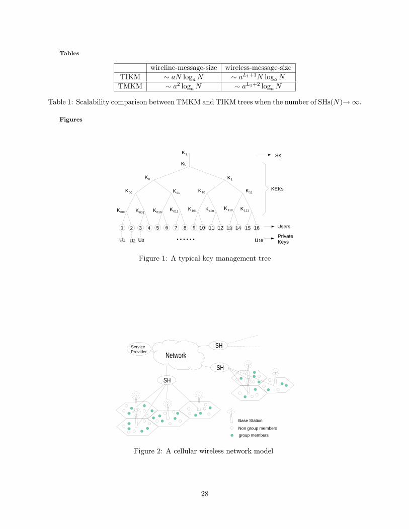
The most common class of multicast key management schemes employ a tree hierarchy of

KEKs [6–10], as depicted in Figure 1. Each user stores his private key ui, the session key Ks, and

a set of KEKs on the path from himself to the root of the key tree. Since the size of the rekeying

messages sent for a member join operation is much less than that for member departure [7,10], we

shall only focus on the communication cost of member departure. For example, referring to Figure

1, when user 16 leaves the multicast service, all of his keys, {u16, Ks,Kε,K1,K11,K111}, should

be updated. Let xold denote the old version of key x, xnew denote the new version of key x, and

{y}x denote the key y encrypted by key x. Then, the key updating can be achieved by sending the

following rekeying messages:

1. {Knew111 }u15 is sent and user 15 acquires Knew

111 .

2. {Knew11 }Knew

111and {Knew

11 }Kold110

are sent and users 13, 14, 15 acquire Knew11 .

3. {Knew1 }Knew

11and {Knew

1 }Kold10

are sent and users 9, 10, · · · , 15 acquire Knew1 .

4. {Knewε }Knew

1and {Knew

ε }Kold0

are sent and users 1, 2, · · · , 15 acquire Knewε .

5. {Knews }Knew

εis sent and users 1, 2, · · · , 15 acquire the new session key Knew

s .

The above key updating procedure achieves key updating without leaking new key information to

the leaving user. This example also illustrates that most rekeying messages are only useful to a

subset of users, who are always neighbors on the key management tree. In fact, the first rekeying

message is only useful to user 15, the second rekeying message is only useful to users 13, 14, 15, the

third rekeying message is useful to users 9, 10, · · · , 15, and the fourth and fifth rekeying messages

are useful to all users. Therefore, rekeying messages do not have to be sent to every user in the

multicast group.

We propose to exploit this observation in designing a key management tree. Our key manage-

ment tree will match the network topology in such a way that the neighbors on the key tree are

3

also physical neighbors on the network. By delivering the rekeying messages only to the users who

need them, we may take advantage of the fact that the key tree matches the network topology, and

localize the delivery of rekeying messages to small regions of the network. This lessens the amount

of traffic crossing portions of the network that do not have users who need to be rekeyed. In order

to accomplish this, it is necessary to have the assistance of entities that would control the rekeying

message transmission, such as the base stations in cellular wireless networks.

A cellular network model, as depicted in Figure 2 and proposed in [16], consists of mobile

users, base stations (BS) and supervisor hosts (SH). The SHs administrate the BSs and handle

most of the routing and protocol details for mobile users. The service provider, the SHs, and

the BSs are connected through high-speed wired connections, while the BSs and the mobile users

are connected through wireless channels. In this paper, the SHs can represent any entity that

administers BSs, such as the region servers presented in [17] or the radio network controllers (RNCs)

in 3G networks [18]. In cellular wireless networks, multicast communication can be implemented

efficiently by exploiting the inherent broadcasting nature of the wireless media [19–21]. In this case,

multicast data is first routed to the BSs using multicast routing techniques designed for wireline

networks [1], and then broadcast by the BSs to mobile users.

If we assume that both the SHs and the BSs can determine whether the rekeying messages are

useful for the users under them, then the cellular wireless network has the capability of sending

messages to a subset of users. In particular, the SHs multicast a rekeying message to their BSs if

and only if the message is useful to one or several of their BSs, and the BSs broadcast the rekeying

message to their users if and only if the message is useful to the users under them. The information

needed to identify whether a SH or BS needs a rekeying message can be sent in the rekeying

message header. We shall not consider the size of this overhead information in our calculation

since this overhead is typically small compared to the size of the actual rekeying messages, and

is implementation-dependent. Hence, when the key tree matches the network topology, we can

localize the delivery of rekeying messages.

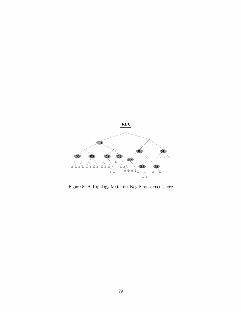
We design a key management tree that matches the network topology in three steps:

• Step 1: Design a subtree for the users under each BS. These subtrees are referred to as user

subtrees.

4

• Step 2: Design subtrees that govern the key hierarchy between the BSs and each SH. These

subtrees are referred to as BS subtrees.

• Step 3: Design a subtree that governs the key hierarchy between the SHs and the KDC. This

subtree is referred to as the SH subtree.

The combined key management tree is called a Topology-Matching Key Management (TMKM)

tree. Figure 3 illustrates a TMKM tree for the network topology shown in Figure 2. Traditional

key management trees, such as those in [7–10], are independent of the network topology, and we

call them Topology Independent Key Management (TIKM) trees. When using a TIKM tree, the

users are scattered all over the network, and therefore it is not possible to localize the delivery of

rekeying messages.

We study the communication burden of the rekeying messages in the wired portion and in the

wireless portion of the network separately. Under each SH, we introduce two costs: the wireline-

message-size, which is defined as the total size of the rekeying messages multicast by the SHs to

the BSs; and the wireless-message-size, which is defined as the total size of the rekeying messages

broadcast by the BSs. The message size is measured in units whose bit length is the same size as

the key length. We note that the wireline message size does not capture all of the wired cost in

the network, as there may be additional wired costs between the SHs and the KDC. This was done

since it is not easy to consider a single formulation for the costs between the SHs and the KDC

that captures the many possible cellular architectures between the KDC and the SHs. On the other

hand, it is possible to use a single formulation to capture the behavior between the SH and the

BS since most cellular systems model the SH-BS connection using a single link, such as the Iub in

3G cellular systems. Further, if we assume that the network connections between the KDC and

the SHs are trivial, that is the KDC is placed at the SHs, or if the network connections between

the KDC and the SHs have ample enough bandwidth resources, then the KDC-SH cost may be

considered negligible compared to the SH-BS costs. Therefore, we have made a simplification to

consider only the SH-BS wired cost and do not consider KDC-SH wired costs in this paper.

Let Sl1 denote the wireline-message-size under the lth SH and Sl

2 denote the wireless-message-size

under the lth SH, where l = 1, 2, · · · , nsh and nsh is the total number of SHs. For example, when the

length of the session key and KEKs is 128 bits each, if a 256 bit long rekeying message is multicast

5

by the lth SH and then broadcast by 3 BSs under the lth SH, then Sl1 = 2 and Sl

2 = 6. Assuming

that users do not leave simultaneously, then the rekeying wireline cost, Cwire, the rekeying wireless

cost Cwireless, and the total rekeying cost CT , are defined as:

Cwire =nsh∑

l=1

αl1E[Sl

1] ; Cwireless =nsh∑

l=1

αl2E[Sl

2]

CT = γ · Cwireless + (1− γ) · Cwire, (1)

where E[.] indicates expectation over the statistics governing the user joining and leaving behavior.

Here, 0 ≤ γ ≤ 1 is the wireless weight, which represents the importance of considering the wireless

cost, and {αl1} and {αl

2} are the sets of weight factors that describe the importance of considering the

wireline-message-size and wireless-messages-size under the lth SH respectively. When SHs admin-

istrate areas with similar physical network structure and channel conditions, we can approximate

{αl1} and {αl

2} by 1. In addition, we define the combined-message-size as SlT = γ·Sl

2αl2+(1−γ)·Sl

1αl1.

Thus, CT can also be expressed as CT =∑nsh

l=1 E[SlT ].

For a given wireless weight γ, {αl1}, and {αl

2}, both the TMKM and TIKM trees should be

designed to minimize the total communication cost, CT .

3 Handoff Schemes for TMKM Tree

In mobile environments, the user will subscribe to a multicast service under an initial host agent,

and through the course of his service move to different cells and undergo handoff to different base

stations. Although the user has moved, he still maintains his subscription to the multicast group.

Since the TMKM tree depends on the network topology, the physical location of a user affects the

user’s position on the key management tree. When a user moves from one cell to another cell, the

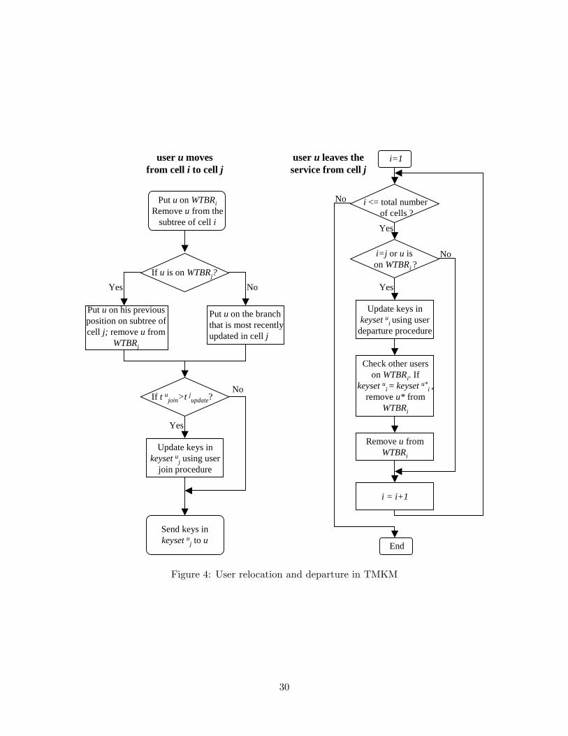
user needs to be relocated on the TMKM tree. In this section, we propose an efficient handoff

scheme for our TMKM trees. In this context, the expression handoff scheme will only refer to the

process of relocating a user on the key tree.

One solution to the handoff problem is to treat the moving user as if he departs the service

from the cell that he is leaving from and then rejoins the service in the cell that he has moved to.

This scheme, referred to as the simple handoff scheme, is not practical for mobile networks with

frequent handoffs since rekeying messages are sent whenever handoffs occur.

6

During handoff, if a user remains subscribed to the multicast group, it is not necessary to

remove the user from the cell where he previously stayed. Allowing a mobile user to have more

than one set of valid keys while he stays in the service does not compromise the requirements of

access control, as long as all of the keys that he possesses are updated when he finally leaves the

service. In order to trace both the users’ handoff behavior and the key updating process, we employ

a wait-to-be-removed (WTBR) list for each cell. The WTBR list of cell i, denoted by WTBRi,

contains the users who (1) possess a set of valid keys on the user subtree of cell i and (2) are

currently in the service but not in cell i. These WTBR lists are maintained by the KDC.

Let tiupdate denote the time of the last key update that occurs due to a departure occurring in

cell i, and let tujoin denote the time when the user u first joins the service. In addition, we define

keysetui to be the set of keys possessed by the user u while he is in cell i. We propose an efficient

handoff scheme that is illustrated in Figure 4, as:

• When user u moves from cell i to cell j,

1. Put u on the WTBR list of cell i, i.e. WTBRi, and remove him from the user subtree

of cell i.

2. If u has been in cell j before and is on WTBRj , put u back on the branch of the subtree

that he previously belonged to and remove him from WTBRj . If u is not on WTBRj ,

put u on the most recently updated branch of the user subtree of cell j. We note that

the set of keys associated with u’s new position, keysetuj , was updated at time tjupdate.

3. If tujoin > tjupdate, the keys in keysetuj are updated using the procedure for user join

described in [10]. If tujoin ≤ tjupdate, the keys do not need to be updated.

4. The keys in keysetuj are sent to u through unicast.

The purpose of step 3 is to prevent u from taking advantage of the handoff process to access

the communication that occurred before he joined. To see this, let u join the service at

tujoin = t0 in cell i, and then immediately move to cell j. After relocation, user u obtains keys

in keysetuj that is updated at time tjupdate = t0 − ∆, where ∆ is a positive number. In this

case, if we do not update the keys in keysetuj and u has recorded the communication in cell

7

j before joining, u will be able to decrypt the multicast content transmitted in [t0 −∆, t0),

during which time he is not a valid group member.

• When user u leaves the multicast service from cell j:

1. The keys that are processed by u and still valid should be updated. In particular, the

keys in keysetuj and {keysetui : WTBRi contains u} are updated using the procedure

for user departure in [10].

2. Check other users on the WTBR lists that contain u. If u and another user u∗ are both

on WTBRi, and keysetui = keysetu∗

i , remove u∗ from WTBRi. It is noted that u∗ is

removed from WTBRi when u∗ does not have valid keys associated with cell i any more.

Step 2 does not require extra rekeying messages.

3. Remove u from all WTBR lists.

Thus, a user will be removed from the WTBR lists not only when he leaves the service, but also

when other users who share the same keys leave the service. Compared with the simple handoff

scheme, the efficient handoff scheme can reduce the key updating caused by user relocation because

the number of cells that need to update keys is smaller than the number of cells that a user has

ever visited.

When the key tree matches the network topology, handoffs result in user relocation on the key

tree, which inevitably introduces extra cost to the task of key management. In this work, we assume

that the KDC has significant computation and storage resources and do not investigate the cost

for the KDC to maintain and update the WTBR lists. We will focus on the extra communication

cost due to the fact that more than one set of keys may need to be updated for a departing user

when handoffs exist.

4 Analysis of the TMKM Tree

Matching the key management tree with the network topology has two contrasting effects on the

rekeying message communication cost. First, the cost of sending one rekeying message is reduced

because only a subset of the BSs broadcast the message. Second, the number of rekeying messages

may increase due to handoffs. In this section, we analyze these two effects and investigate the

8

influence that user mobility and the wireless weight have upon the performance of the TMKM

scheme.

To simplify the analysis, we assume that the system has aL0 SHs, each SH administrates aL1

BSs, and each BS has aL2 users, where a ≥ 2, L0, L1 and L2 are positive integers. We also assume

that the SHs administer areas with similar network structure and conditions. Therefore, {αl1} and

{αl2} are approximated by 1. The user subtrees, BS subtrees, and SH subtree are designed as

balanced trees with degree a and level L2, L1, and L0, respectively. For fair comparison, the TIKM

tree is also designed as an a-ary balanced tree with (L0 +L1 +L2) levels. In this work, the level of a

tree is defined as the maximum number of nodes on the path from a leaf node to the root excluding

the leaf node. Since the SHs are usually in charge of large areas, the probability of a user moving

between SHs during a multicast service is much smaller than the probability of handoffs that are

under one SH. In this analysis, we assume that there are no SH level handoffs. For the present

computation, we only calculate the communication cost caused by one departing user based on the

rekeying procedure described in [6, 7, 10].

As illustrated by the example in Section 2, rekeying messages of size (a·L) need to be transmitted

when one user leaves from a balanced key tree with degree a and level L. When using the TIKM

tree, rekeying messages of size a(L0 + L1 + L2) are transmitted under aL0 SHs and broadcast by

aL0+L1 BSs. Therefore, when one user leaves the service, the wireline-message-size, denoted by

Ctikmw , and the wireless-message-size, denoted by Ctikm

wl , are computed as:

Ctikmw = (aL0 + aL1 + aL2)aL0 (2)

Ctikmwl = (aL0 + aL1 + aL2)aL0+L1 . (3)

The performance of the TMKM tree is affected by the user handoff behavior. We define the

random variable I as the number of WTBR lists that contain the departing member when he leaves

the service. We also introduce the function B(b, i, a) that describes the number of intermediate

KEKs that need to be updated. B(b, i, a) is equivalent to the expected number of occupied boxes

when putting i items in b boxes with repetition, where each box can have at most a items. A box is

called occupied when one or more items are put into the box. The detailed calculation of B(b, i, a)

is given in Appendix A.

When one user leaves the service and he is on I = i WTBR lists, we can show that:

9

• We need to update (i · L2) keys on the user subtrees. Thus, rekeying messages with a total

size (iaL2 − 1) are transmitted under one SH and broadcast by a single BS.

• We need to update B(aL1−m, i, am) KEKs on the level (L1 − m) of the BS subtree. Thus,

messages with size aB(aL1−m, i, am) are transmitted under one SH and broadcast by am BSs.

Here, m = 1, · · · , L1, and the level 0 of a tree is just the root.

• We need to update (at) KEKs on the level (L0 − t) of the SH subtree. Thus, messages with

size (at+1) are sent under (at) SHs and broadcast by (aL1 · at) BSs. Here, t = 1, 2, · · · , L0.

• In addition, we need one message to update the session key Ks. This message is sent to all

aL0 SHs and aL0+L1 BSs.

Therefore, when the departing user belongs to i WTBR lists, the expected value of the wireline-

message-size, denoted by Ctmkmw (i), and the expected value of the wireless-message-size, denoted

by Ctmkmwl (i), are computed as:

Ctmkmw (i) = iaL2 +

L1∑

m=1

aB(aL1−m, i, am) +L0∑

t=1

at+1 (4)

Ctmkmwl (i) = iaL2 − 1 +

L1∑

m=1

am+1B(aL1−m, i, am) + aL1

L0∑

t=1

at+1 + aL0+L1 . (5)

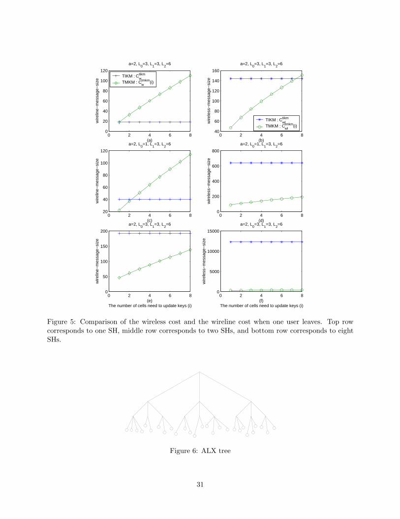
The performance of the TIKM tree and the TMKM tree can be compared by examining the

values of Ctikmw and Ctmkm

w (i), Ctikmwl and Ctmkm

wl (i). In Figure 5, these values are plotted for

different i and L0, when the other parameters are fixed as a = 2, L1 = 3, and L2 = 6. Since the

TIKM tree is not affected by handoffs, Ctikmw and Ctikm

w are constant. Figure 5(a) and Figure 5(b)

show the wireline-message-size and wireless-message-size respectively, when the system has only

one SH. Figure 5(c) and Figure 5(d) show the corresponding curves for 2 SHs, while Figure 5(e)

and Figure 5(f) depict the corresponding curves for systems with 8 SHs. We observe that:

• Both Ctmkmw (i) and Ctmkm

wl (i) are increasing functions of i.

• The TMKM tree always reduces the wireless-message-size, and this advantage becomes larger

when the system contains more SHs.

• For systems containing only one SH, i.e. L0 = 0, the TMKM trees introduce larger wireline-

message-sizes than TIKM trees due to the handoff effects. When there are multiple SHs,

10

the TMKM scheme can take advantage of the fact that some SHs do not need to transmit

rekeying messages to their BSs, and can reduce the wireline-message-size when i is small. It

should be noted that the wireline cost will be larger than that given in (4) if there are SH-level

handoffs.

Since TMKM trees reduce the wireless-message-size more effectively than reducing the wireline

message size, a larger wireless weight γ leads to an improved advantage of TMKM trees over TIKM

trees. Using large γ is reasonable since the wireless portion of the network usually experiences a

higher error rate and has less available bandwidth when compared to the wireline portion, which

makes the wireless cost the major concern in many realistic systems. In addition, the communication

cost of the TMKM tree increases with the number of cells that need to update keys when a user

leaves. Therefore, when handoffs are less likely to happen, the TMKM tree has larger advantage

over the TIKM tree.

Scalability is another important performance measure of key management schemes [6]. We

define N = aL0 as the number of SHs. When N → ∞, the scalability properties can be easily

obtained from (2)-(5), and are summarized in Table 1. Both Figure 5 and Table 1 demonstrate

that the communication cost of TMKM trees scales better than that of TIKM trees when more

SHs participate in the multicast service.

5 Separability of the Optimization Problem

The TMKM tree consists of user-subtrees, BS-subtrees, and SH-subtrees. In this section, we show

that optimizing the entire TMKM tree is equivalent to optimizing those subtrees individually. This

is desirable since optimizing the subtrees separately reduces the dimension of the search space for

optimal tree parameters and significantly reduces the complexity of tree design.

In this work, we assume that the users under the same SH have the same joining, departure and

mobility behavior. Thus, the user subtrees under the same SH have the same structure. It is easy

to verify that the main results in this section still hold in scenarios where the dynamic behavior of

the users varies under different BSs. However, for the discussion in this paper, we will restrict our

attention to the case where the dynamic behavior of the users between different BSs is identical.

In addition, we assume that the number of participating SHs and BSs do not change during the

11

multicast service. In order to make the presentation more concise, we introduce the notation Dk,l

to represent the situation where k users are under the lth SH and one of these users leaves the

service.

As discussed in Section 2, the total communication cost, CT , is expressed as

CT =nsh∑

l=1

E[SlT ]. (6)

Based on the definition of SlT , one can see that

E[SlT ] =

∑

k

pl(k)Gl(k)El(k), (7)

where

pl(k) : pmf of the number of users under the lth SH,

Gl(k) : probability that a user leaves from the lth SH given that k users are under the lth SH,

El(k) : the expected value of the combined-message-size given the condition Dk,l.

When a user leaves, the keys that need to be updated are divided into three categories: (1) the

keys on the user subtrees, (2) the keys on the BS subtrees, and (3) the keys on the SH subtree.

Under the condition Dk,l, let Al1(k), Al

2(k) and Al3 denote the expected value of the combined-

message-size under the lth SH resulting from updating the keys on the user-subtrees, BS-subtrees

and SH-subtrees, respectively. We note that Al3 is not a function of k when there are no SH-level

handoffs, and that El(k) = Al1(k) + Al

2(k) + Al3. Then, (6) becomes

CT =nsh∑

l=1

(∑

k

pl(k)Gl(k)Al1(k)

)+

nsh∑

l=1

(∑

k

pl(k)Gl(k)Al2(k)

)+

nsh∑

l=1

Al3 ·

(∑

k

pl(k)Gl(k)

). (8)

We observe that the structure of the user-subtrees only affects Al1(k), the structure of the

BS-subtrees only affects Al2(k), and the structure of the SH-subtrees only affects Al

3. There-

fore, for the TMKM tree, the user-subtrees, BS-subtrees and SH subtree can be designed and

optimized separately. Particularly, the user-subtrees under the lth SH should be designed to

minimize∑

k pl(k)Gl(k)Al1(k), the BS subtree under the lth SH should be designed to minimize

∑k pl(k)Gl(k)Al

2(k), and the SH subtree should be designed to minimize∑nsh

l=1 Al3 ·

(∑k pl(k)Gl(k)

).

12

6 Design of the TMKM Tree

Key management schemes are closely related to the key management architecture, which describes

the entities in the network that perform key management [6]. In cellular wireless networks, the BSs

are not trusted to perform key management because they can be easily tampered with [16]. The

SHs are able to perform key management if they are trusted and have the necessary computation

and storage capabilities. The trustiness of the SHs depends on both the business model and the

protection on the SHs. Based on whether SHs perform key management, the systems can be

classified into two categories:

• In the first category, each SH performs key management for a subset of the group members

who reside in the region where this SH is in charge. Each SH can be looked at as a local

key distribution center (KDC). Without loss of generality, since the SHs are independent and

may even adopt different key management schemes, we can study systems containing only

one SH, which we shall refer to as one-SH systems.

• In the second category, SHs do not perform key management. Instead, there is a single KDC

that manages keys for all of the users. This KDC can be the service provider or a trusted

third party. The systems containing many SHs are referred to as multiple-SH systems.

In one-SH systems, the TMKM tree consists of user-subtrees and a BS subtree. In multiple-SH

systems, the TMKM tree consists of user-subtrees, BS-subtrees and a SH subtree.

In this section, we introduce a model describing the joining and leaving behavior of the users,

and a flexible tree structure that can be used to design the user and BS subtrees. We then examine

the optimization of the user and BS subtrees and the design of the SH subtree.

6.1 Dynamic membership model

Mlisten [22] is a tool that can collect the join/leave times for multicast group members in MBone

sessions. Using this tool, [23,24] studied the characteristics of the membership dynamics of MBone

multicast sessions and showed that the user arrival process can be modeled as Poisson and the

membership duration of short sessions (that usually last several hours) is accurately modeled using

an exponential distribution while the membership duration of long sessions (that usually last several

13

days) is accurately modeled using the Zipf distribution [25]. Based on the population model of short

MBone sessions, we made the following assumptions on the membership dynamics:

1. Under the lth SH, the user’s arrival process is Poisson with rate λl and the service duration

is governed by an exponential random variable with mean 1/µl, where l = 1, 2, · · · , nsh.

2. A user’s joining and leaving behavior is independent of other users.

Based on the first assumption, the number of users under the lth SH is a Poisson random variable

with rate θl, i.e. pl(k) = θkl

k! e−θl , where θl = λl/µl [26]. In addition, it can be shown that Gl(k)

approximately equals to k · µl. It is noted that the second assumption is reasonable in some types

of multicast services, such as periodic news multicast, while it may not be correct for services such

as a scheduled pay-per-view multicast, where different users are related with each other through

watching the same content.

In this work, we use this Poisson arrival and exponential service duration model to optimize

the TMKM tree. In Section 7, we will use simulations to demonstrate that the performance of the

TMKM tree is not sensitive to users’ statistical membership models.

6.2 ALX tree structure

The TMKM scheme matches the key tree to the network topology by decomposing the key tree

into user subtrees, BS subtrees, and SH subtrees. The TMKM scheme does not have constraints

on the specific structure of these subtrees. In this section, we propose a tree structure that is

capable of handling membership additions, deletions, or relocations with minimal changes to the

tree’s structure.

As illustrated in Figure 6 and parameterized by the triple (a, L,x), this (a, L,x)-logical tree has

L + 1 levels. The upper L levels, which comprise a full balanced subtree with degree a, are fixed

during the multicast service. The users are represented by the leaf nodes on the (L+1)st level. We

use a vector x to describe the (L+1)st level, where xi is the number of users attached to the ith node

of the Lth level, and i = 1, 2, · · · , aL. In the example shown in Figure 6, x = [4, 2, 3, 3, 2, 4, 3, 3, 3],

a = 3 and L = 3. We will refer to this tree structure as the ALX tree.

When using the ALX tree, the joining user is always put on the branch with the smallest value

of xi. The maximum number of users on an ALX tree is not restricted. When a user leaves,

14

the average rekeying message size is ( kaL − 1 + aL), where k is the number of users on the ALX

tree. When the user’s arrival process is Poisson with rate λ, and the service time is an exponential

random variable with mean 1/µ, the probability that a user leaves the key tree is approximately

k · µ, and the pmf of k is p(k) = θk

k! e−θ, where θ = λ/µ. The performance of the ALX tree is

evaluated by the expected value of the rekeying message size, denoted by Calx, and is calculated as

Calx =∞∑

k=1

p(k) · k · µ · ( k

aL− 1 + aL). (9)

It follows that the optimization problem of the ALX tree can be formulated as:

Calx = mina>1,L>0

Calx. (10)

Balanced trees whose degree is pre-determined, such as binary and trinary trees, are widely

used to design key trees [6,10]. Next, we compare the ALX tree structure with balanced trees that

have a pre-defined degree, which we refer to as fixed-degree trees in this section.

Adding or removing a user from balanced fixed-degree trees often requires splitting or merging

nodes. For example, when a new user is added to the key tree shown in Figure 1, one leaf node

must be split to accommodate the joining user. In this case, a new KEK is created and must be

transmitted to at least one existing user. When using the ALX tree structure, however, no new

KEKs are created during membership changes. We know that updating existing KEKs for user

join can be achieved without sending any rekeying messages, as suggested in [10], because existing

users can update KEKs using one-way functions after being informed of the need to update their

keys. Therefore, the ALX tree structure allows for a key updating operation that does not require

sending any rekeying messages during user joins. In addition, the ALX tree introduces minimal

change to the tree structure with dynamic membership and therefore is easy to implement and

analyze.

Further, the ALX tree should be optimized over the distribution of the group size. If we take

individual snapshots of the system when the group size is very small or large, the ALX tree may not

perform as well as fixed degree trees that adjust themselves according to the group size. However,

we will derive the performance lower bound for fixed degree trees and then demonstrate that the

cost for ALX trees, Calx, is in fact very close to this lower bound. Similar to (9), the expected

15

rekeying message size when using a tree with fixed degree n, denoted by Cfix(n), is calculated as:

Cfix(n) =∞∑

k=1

p(k) · k · µ(n− 1 + n · (P − 1)) ,

where P is the average length of branches for a tree with k leaves and degree n. It is well known

that P equals the expected codeword length of a source code containing k symbols with equal

probability. The bounds on P are known to be logn(k) ≤ P < logn(k) + 1 [27]. Therefore,

Cfix(n) >∞∑

k=1

p(k) · k · µ · (n logn(k)− 1). (11)

Based on (11), the performance lower bound for the fixed degree trees is given by

Cfix = minn

∞∑

k=1

p(k) · k · µ · (n logn(k)− 1). (12)

It is noted that no fixed degree trees can reach this lower bound. In fact, Cfix would be achieved

if and only if we could (1) reorganize the tree immediately after user join or departure in such a

way that the rekeying message size for the next user join/leave operation is minimized; and (2)

reorganize the tree without adding any extra communication cost. However, reorganizing trees,

such as splitting or merging nodes, requires sending extra keying information to users. These above

two conditions can never be achieved simultaneously.

The lower bound in (12) is used as a reference for evaluating the performance of the ALX tree.

In Figure 7(a), Cfix and Calx are compared for different user joining rates, λ. In Figure 7(b), Cfix

and Calx are compared for different average service durations, 1/µ. We observe that the relative

difference between the lower bound and the performance of the ALX tree is less than 3.5%.

The ALX tree has the advantage of maintaining tree structure during user joins and departures,

while its performance is very close to the lower bound of fixed degree trees. Although ALX tree is

not the optimal solution amongst all possible tree structures, its practical nature makes the ALX

tree an ideal candidate for designing the user and BS subtrees.

6.3 User Subtree Design

The user subtrees are designed as ALX trees. Under the lth SH, the optimal tree parameters, a

and L, solve

mina,L

∑

k

pl(k)Gl(k)Al1(k), (13)

16

where a and L are positive integers and Gl(k) ≈ kµl. Let T uw(k, i) and T u

wl(k, i) respectively represent

the expected value of the wireline-message-size and wireless-message-size caused by updating keys

on the user subtrees, given that k users are under the lth SH, one of them leaves and he is on i

WTBR lists. We can show that

T uw(k, i) = T u

wl(k, i) = (k/nl

bs

aL− 1 + aL)i.

Then, Al1(k) is computed as

Al1(k) =

nlbs∑

i=1

plh(i)(αl

2γT uwl(k, i) + αl

1(1− γ)T uw(k, i))

= (αl2γ + αl

1(1− γ))(k/nl

bs

aL− 1 + aL)E[I l], (14)

where E[I l] =∑nl

bsi=1 pl

h(i)i, and αl1 and αl

2 are defined in Section 2. By substituting (14) into (13),

the optimization problem for the user-subtrees under the lth SH is

mina,L

∑

k

k · pl(k) · (k/nlbs

aL− 1 + aL). (15)

The optimum a and L can be obtained by searching the space of possible a and L values.

6.4 BS Subtree Design

We also design BS subtrees as ALX trees. We denote the degree and the level of a BS subtree by

abs and Lbs, respectively. Let T bw(k, i) and T b

wl(k, i) respectively denote the expected value of the

wireline-message-size and wireless-message-size caused by key updating on the BS subtree under

the lth SH given the condition Dk,l and the condition that the departing member is on i WTBR

lists. We can show that:

T bw(k, i) = s ·B(abs

Lbs , i, s) +Lbs∑

m=1

abs ·B(absLbs−m, i, s · am

bs) (16)

T bwl(k, i) ≈ s2 ·B(abs

Lbs , i, s) +Lbs∑

m=1

abs · absm · s ·B(abs

Lbs−m, i, s · ambs), (17)

where s = nlbs

aLbsbs

. Equation (16) and (17) are derived based on the following intermediate results:

• On average, B(absLbs−m, i, s·am

bs) keys need to be updated on level (Lbs−m) of the BS subtree.

17

• To update one KEK at level Lbs, the average message size is (s) and these messages are

broadcast to an average of (s) BSs. To update one KEK at level (Lbs − m),m > 0, the

message size is (abs) and these messages are broadcast by (ambs) BSs.

From the definition of Al2 and using both (16) and (17), we can see that

Al2 =

nlbs∑

i=1

plh(i)(αl

2γT bwl(k, i) + αl

1(1− γ)T bw(k, i))

=nl

bs∑

i=1

plh(i)

(B(abs

Lbs , i, s)(s2αl

2γ + sαl1(1− γ)

)

+Lbs∑

m=1

B(absLbs−m, i, s · am

bs)abs

(abs

msαl2γ + αl

1(1− γ)) , (18)

where nlbs is the number of BSs under the lth SH. In practice, it is difficult to obtain an analytic

expression for plh(i) that depends on the statistical behavior of the users during membership joins

and departures, as well as their mobility behavior and how handoffs are addressed. Thus, we

introduce random variable I l, which is the number of cells that a leaving user has ever visited.

Obviously, I l ≥ I l. The pmf of I l, denoted by plh(i) , can be derived from user mobility behavior

and the distribution of the service duration, as described in Appendix B. Let Al2 denote the right

hand side of (18) when replacing plh(i) by pl

h(i). We can show that Al2 is an upper bound of Al

2.

We notice that Al2 is not a function of k.

As discussed in Section 5, the parameters of the BS subtree under the lth SH should be chosen

such that∑

k pl(k)Gl(k)Al2 is minimized. Since Gl(k) is not a function of abs and Lbs, minimizing

∑k pl(k)Gl(k)Al

2 is equivalent to minimizing Al2. Due to the unavailability of pl

h(i), we choose the

parameters of the BS subtrees under the lth SH that minimize the upper bound of Al2, as:

minabs>1,Lbs>0

Al2. (19)

6.5 SH Subtree Design

In a typical cellular network, each SH administrates a large area where both the user dynamics

and the network conditions may differ significantly from the areas administered by other SHs. The

heterogeneity among the SHs should be considered when designing the SH subtree. Due to SH

heterogeneity, the ALX tree structure, which treats every leaf equally, is not an appropriate tree

18

structure to build the SH subtree. Instead, the SH heterogeneity may be addressed by building a

tree where the SHs have varying path lengths from the root to their leaf node. In this section, we

will first formulate the SH subtree design problem and then provide a sub-optimal tree generation

procedure.

The root of the SH subtree is the KDC, and the leaves are the SHs. The design goal is to

minimize the third term in equation (8), which shall be denoted by Csh and is given by

Csh =nsh∑

l=1

ql ·Al3, (20)

where ql =∑

k pl(k)Gl(k). Let βl denote the communication cost of transmitting one rekeying

message to all the users under the lth SH. Based on the definition of αl1 and αl

2 in Section 2, it is

easy to show that βl = (1− γ)αl1 + γnl

bsαl2.

The value of Al3 can be calculated directly from βl where l = 1, 2, · · · , nsh. In the simple

example demonstrated in Figure 8, when a user under SH1 leaves the multicast service, K00, K0,

Kε and Ks, need to be updated. The communication cost of updating K00 is 2(β1 + β2). The

communication cost of updating K0 is 2(β1 + β2 + β3). The communication cost of updating Kε is

2(β1 + β2 + β3 + β4 + β5). Since the communication cost of updating Ks does not depend on SH

subtree structure, it is not counted in the total communication cost. Then, we have:

A13 = 2(β1 + β2) + 2(β1 + β2 + β3) + 2(β1 + β2 + β3 + β4 + β5).

The goal of SH subtree design is to find a tree structure that minimizes Csh given βl and ql.

However, it is very difficult to do so based on (20). Thus, we compute Csh in a different way.

We assume that the SH subtree has the fixed degree n. We shall assign a cost pair, which is

a pair of positive numbers, to each node on the tree as follows. The cost pair of the leaf node

that represents the lth SH is (ql, βl). The cost pair of the intermediate nodes are the element-wise

summation of their children nodes’ cost pairs, as illustrated in Figure 9. The cost pairs of all

intermediate nodes are represented by (xm, ym), where m = 1, 2, · · · ,M , and M is the total number

of intermediate nodes on the tree. Then, Csh can be calculated as:

Csh = nM∑

m=1

xm · ym. (21)

It is easy to verify that (21) is equivalent to (20). Based on (21), we propose a tree construction

method for n = 2 as:

19

1. Label all the leaf nodes using their cost pairs, and mark them to be active nodes.

2. Choose two active nodes, (xi, yi) and (xj , yj), such that (xi+xj) ·(yi+yj) is minimized among

all possible pairs of active nodes. Mark those two nodes to be inactive and merge them to

generate a new active node with the cost pair (xi + xj , yi + yj).

3. Repeat step 2 until there is only one active node left.

This method, which we call the greedy-SH subtree-design (GSHD) algorithm, can be easily extended

to n > 2 cases. We can prove that the GSHD algorithm produces the optimal solution when

β1 = β2 = · · ·βnsh, but is not optimal in general cases. Since the optimization problem for the SH-

subtree is non-linear, combinatorial, and even does not have a closed expression for the objective

function, we do not seek the optimal SH subtree structure in this paper. In Section 7, we will

compare the performance of the GSHD algorithm and the optimal solution obtained by exhaustive

search.

7 Simulation Results

7.1 One-SH Systems

We first compare the performance of the TMKM tree and the TIKM tree in one-SH systems using

both analysis and simulations. Similar to [28, 29], we employ a homogeneous cellular network

that consists of 12 concatenated cells, and wrap the cell pattern to avoid edge effects. We use

the mobility model proposed in [30], where R denotes the radius of the cells, and Vmax denotes

the maximum speed of the mobile users. Since the wireless connection usually experiences a high

transmission error rate and the number of users under one BS is larger than the number of BSs,

the wireless communication cost of the multicast communication is assigned a larger weight than

the wireline communication cost, i.e. γ > 0.5.

For the purpose of fair comparison, the TIKM tree is designed as an ALX tree, which is optimized

for the statistics of the number of participating users. The wireline cost of the TIKM tree, denoted

by Ctikmwire , is computed using (9), where p(k) denotes the pmf of the number of users in the multicast

service. The wireless cost of the TIKM tree is computed as Ctikmwireless = nbsC

tikmwire , where nbs is the

total number of BSs. In one-SH systems, the total communication cost is CtikmT = γCtikm

wireless +

20

(1 − γ)Ctikmwire . We define the performance ratio η as the total communication cost of the TMKM

tree divided by the total communication cost of the TIKM tree, i.e. η = CtmkmT /Ctikm

T . When η is

less than 1, the TMKM tree has smaller communication cost than the TIKM tree, and smaller η

indicates an improved advantage that the TMKM tree has over the TIKM tree.

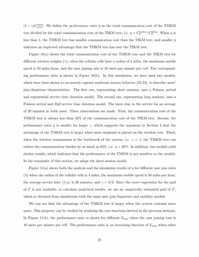
Figure 10(a) shows the total communication cost of the TMKM tree and the TIKM tree for

different wireless weights (γ), when the cellular cells have a radius of 4 miles, the maximum mobile

speed is 50 miles/hour, and the user joining rate is 16 users per minute per cell. The correspond-

ing performance ratio is shown in Figure 10(b). In this simulation, we have used two models,

which have been shown to accurately capture multicast session behavior [23,24], to describe users’

join/departure characteristics. The first one, representing short sessions, uses a Poisson arrival

and exponential service time duration model. The second one, representing long sessions, uses a

Poisson arrival and Zipf service time duration model. The users stay in the service for an average

of 20 minutes in both cases. Three observations are made. First, the communication cost of the

TMKM tree is always less than 42% of the communication cost of the TIKM tree. Second, the

performance ratio η is smaller for larger γ, which supports the argument in Section 4 that the

advantage of the TMKM tree is larger when more emphasis is placed on the wireless cost. Third,

when the wireless transmission is the bottleneck of the system, i.e. γ = 1, the TMKM tree can

reduce the communication burden by as much as 65%, i.e. η = 35%. In addition, two models yield

similar results, which indicates that the performance of the TMKM is not sensitive to the models.

In the remainder of this section, we adopt the short session model.

Figure 11(a) shows both the analysis and the simulation results of η for different user join rates

(λ) when the radius of the cellular cells is 4 miles, the maximum mobile speed is 50 miles per hour,

the average service time (1/µ) is 20 minutes, and γ = 2/3. Since the exact expression for the pmf

of I l is not available, to calculate analytical results, we use an empirically estimated pmf of I l,

which is obtained from simulations with the same user join/departure and mobility models.

We can see that the advantage of the TMKM tree is larger when the system contains more

users. This property can be verified by studying the cost functions derived in the previous sections.

In Figure 11(b), the performance ratio is shown for different Vmax when the user joining rate is

16 users per minute per cell. The performance ratio is an increasing function of Vmax when other

21

parameters are fixed since handoffs occur more frequently as users move faster.

7.2 Multiple-SH Systems

As discussed in Section 6, when the system contains multiple SHs and the SHs do not perform key

management, the design the TMKM tree should consider the topology of the SHs.

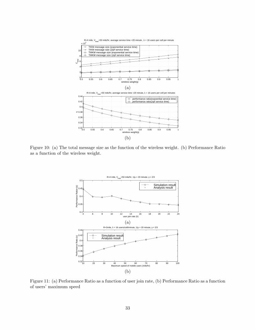
7.2.1 SH subtree design methods

In this section, we compare the GSHD algorithm with the optimal tree obtained by exhaustive

search, and with a balanced tree that treats the SHs equally and represents traditional key man-

agement schemes. We assume that half of the {βl} are uniformly distributed between 1 and 20,

which represent rural areas, and the other half of {βl} uniformly distributed between 101 and 120,

which represent metropolitan areas. We also assume that ql, which is defined in Section 6.5 and

represents the probability of a user leaving, is proportional to βl, where l = 1, 2, · · · , nsh. Here,

{ql} are normalized such that∑

ql = 1. In Figure 12, the communication cost caused by updating

keys on SH-subtrees, Csh, is shown when using different SH subtrees. Results are averaged over

500 realizations. Since exhaustive search is very computationally expensive, it is only done for 10

and fewer SHs. The simulation results indicate that the performance of the GSHD is very close to

optimal. Compared with the balanced tree, the GSHD algorithm reduces the communication cost

contributed by the SH subtree by up to 18%.

7.2.2 Performance of TMKM trees and TIKM trees in multiple-SH systems

For the TMKM trees in multiple-SH systems, we designed the user-subtrees and BS-subtrees as

ALX trees, while the SH-subtrees were constructed using the GSHD algorithm. We simulated a

multiple-SH system where each SH administers 12 concatenated identical cells. The SH-subtrees

are constructed as binary trees. We first study a simple case where the user statistics and network

conditions are identical under all SHs. In this case, αl1’s and αl

2’s are set to be 1. The radius of the

cells is R = 4 miles, the maximum velocity is Vmax = 50 miles/hr, and we also choose µl = 1/30

and λl = 10 for all SHs.

In Figure 13, the wireless cost and the wireline cost of the TMKM trees and the TIKM tree

are shown for different quantities of participating SHs. We observed that the TMKM trees have

22

both smaller wireless cost and smaller wireline costs than the TIKM trees when the number of SHs

are equal or greater than 2, and the advantages of the TMKM trees are more significant when the

system contains more SHs, which verifies the analysis in Section 4. In addition, the corresponding

performance ratio is drawn in Figure 14 for γ = 2/3. In this system, the communication cost of the

TMKM trees can be as low as 20% of the communication cost of the TIKM trees. This indicates

an 80% reduction in the communication cost.

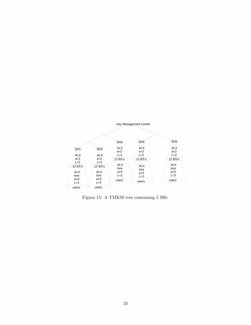
A more complicated system containing 5 SHs with different user joining rates was also simulated.

In this scenario, the λl values for the five SHs were set to 5, 10, 15, 20 and 25 respectively, and

R = 4 miles, Vmax = 50 miles/hr, and µl = 1/20 for all SHs. The TMKM tree structure is shown

in Figure 15. The TIKM tree is simply an ALX tree with degree 3 and level 6. In this system,

the wireless cost of the TMKM tree is 21.8% of that of the TIKM tree, and the wireline cost of

the TMKM tree is 34.0% of that of the TIKM tree. When the wireless weight γ is set to 2/3, the

TMKM tree reduced total communication cost by 74%.

8 Conclusion

In this paper, we presented a method for designing the multicast key management tree for the mo-

bile wireless environment. By matching the key management tree to the cellular network topology

and localizing the delivery of rekeying messages, a significant reduction of 55-80% in the commu-

nication burden associated with rekeying was observed compared to trees that are independent of

the topology.

We designed a topology-matching key management (TMKM) tree that consists of user-subtrees,

BS-subtrees and SH-subtrees. It was shown that the problem of optimizing the communication

cost for the TMKM tree is separable and can be solved by optimizing each of those subtrees

separately. The ALX tree structure, which easily adapts to changes in the number of users, was

introduced to build user-subtrees and BS-subtrees. The performance of the ALX tree is very close

to the performance lower bound for any fixed degree tree. The GSHD algorithm, which considers

the network heterogeneity where the SHs administer areas with varying network conditions, was

introduced to build the SH subtree. The performance of the GSHD algorithm is very close to optimal

and has better performance than treating SHs equally. Additionally, we addressed the consequences

23

that user mobility has upon the topology-matching key management tree, and presented an efficient

handoff scheme to reduce the communication burden associated with rekeying.

A popular user joining/leaving procedure was used to study the performance of the TMKM and

TIKM trees. Both simulations and analysis were provided. For systems consisting of only one SH,

simulations performed for different user-join rates and mobile user speeds show that the cost of the

TMKM tree is approximately 33-45% of the cost of the TIKM tree, which indicates a reduction of

55-67% in the total communication cost. For systems consisting of multiple SHs, simulations were

performed for different amounts of participating SHs, and indicated that the TMKM tree can reduce

the communication burden by as much as 80%. In addition, both analysis and simulations indicate

that the communication cost of the TMKM tree scales better than that of topology-independent

trees as the number of participating SHs increases.

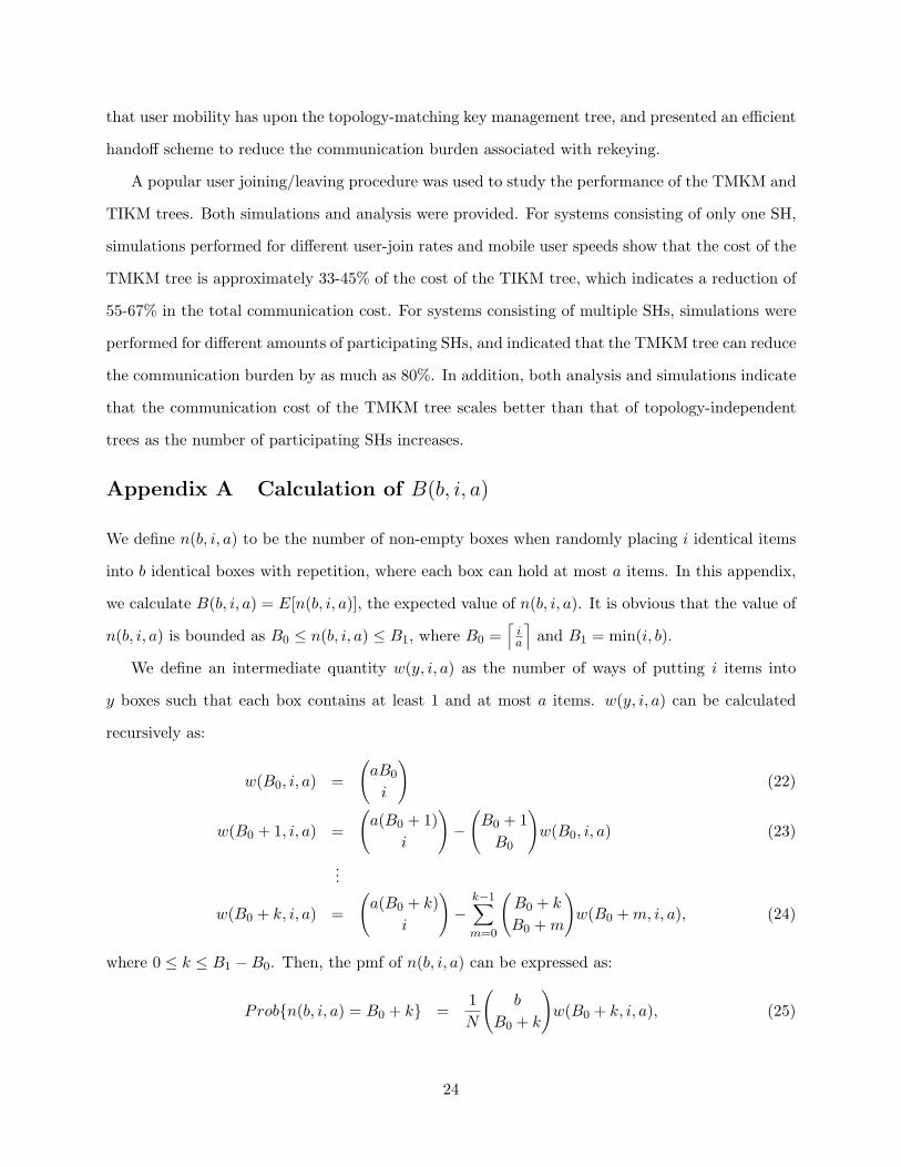
Appendix A Calculation of B(b, i, a)

We define n(b, i, a) to be the number of non-empty boxes when randomly placing i identical items

into b identical boxes with repetition, where each box can hold at most a items. In this appendix,

we calculate B(b, i, a) = E[n(b, i, a)], the expected value of n(b, i, a). It is obvious that the value of

n(b, i, a) is bounded as B0 ≤ n(b, i, a) ≤ B1, where B0 =⌈

ia

⌉and B1 = min(i, b).

We define an intermediate quantity w(y, i, a) as the number of ways of putting i items into

y boxes such that each box contains at least 1 and at most a items. w(y, i, a) can be calculated

recursively as:

w(B0, i, a) =

(aB0

i

)(22)

w(B0 + 1, i, a) =

(a(B0 + 1)

i

)−

(B0 + 1

B0

)w(B0, i, a) (23)

...

w(B0 + k, i, a) =

(a(B0 + k)

i

)−

k−1∑

m=0

(B0 + k

B0 + m

)w(B0 + m, i, a), (24)

where 0 ≤ k ≤ B1 −B0. Then, the pmf of n(b, i, a) can be expressed as:

Prob{n(b, i, a) = B0 + k} =1N

(b

B0 + k

)w(B0 + k, i, a), (25)

24

where N =(ab

i

)represents the total number of ways of putting i items into b boxes. By substituting

(24) into (25), we get:

Prob{n(b, i, a) = B0 + k}

=1N

(b

B0 + k

)(a(B0 + k)

i

)−

k−1∑

m=0

( bB0+k

)(B0+kB0+m

)( bB0+m

) Prob{n(b, i, a) = B0 + m}.

It can be shown that: ( bB0+k

)(B0+kB0+m

)( bB0+m

) =

(b−B0 −m

k −m

).

Therefore,

Prob{n(b, i, a) = B0 + k}

=1N

(b

B0 + k

)(a(B0 + k)

i

)−

k−1∑

m=0

(b−B0 −m

k −m

)Prob{n(b, i, a) = B0 + m}. (26)

By substituting (22) into (25), we have:

Prob{n(b, i, a) = B0} =1N

(b

B0

)(aB0

i

). (27)

Based on (26) and (27), we can calculate Prob{n(b, i, a) = B0 + k} for k = 0, 1, · · · , B1 − B0

recursively. Then, we can calculate B(b, i, a) as:

B(b, i, a) = E[n(b, i, a)] =B1−B0∑

k=0

(B0 + k) · Prob{n(b, i, a) = B0 + k}. (28)

Appendix B Calculation of pmf of I in Section 6.4

Let tM denote the service duration, tn denote the new cell dwell time, and th denote the previously

handed-off cell dwell time [30]. We assume that tM follows exponential distribution. The distribu-

tions of tn and th are often presented together with the mobility models. For the mobility model

used in Section 7, the distribution of tn and th can be found in [30].

Using these distributions, we can calculate pn = Prob{tM < tn} and ph = Prob{tM < th}.The number of cells that a user ever visited before departure, denoted by I, has the pmf as

Prob{I = 1} = pn, Prob{I = 2} = (1 − pn)ph, Prob{I = 3} = (1 − pn)(1 − ph)ph, and Prob{I =

i} = (1− pn)(1− ph)i−2ph.

25

References

[1] S. Paul, Multicast on the Internet and its applications, Kluwer Academic Publishers, 1998.

[2] C. Diot, B.N. Levine, B. Lyles, H. Kassem, and D. Balensiefen, “Deployment issues for the IP multicast serviceand architecture,” IEEE Network, vol. 14, pp. 78 –88, Jan.-Feb 2000.

[3] A. Acharya and B.R. Badrinath, “A framework for delivering multicast messages in networks with mobile hosts,”Journal of Special Topics in Mobile Networks and Applications, vol. 1, no. 2, pp. 199–219, Oct. 1996.

[4] H-S Shin and Y-J Suh, “Multicast routing protocol in mobile networks,” Proc. IEEE International Conferenceon Communications, vol. 3, pp. 1416 –1420, June 2000.

[5] D.M. Wallner, E.J. Harder, and R.C. Agee, “Key management for multicast: issues and architectures,” InternetDraft Report, Sept. 1998, Filename: draft-wallner-key-arch-01.txt.

[6] M.J. Moyer, J.R. Rao, and P. Rohatgi, “A survey of security issues in multicast communications,” IEEENetwork, vol. 13, no. 6, pp. 12–23, Nov.-Dec. 1999.

[7] C. Wong, M. Gouda, and S. Lam, “Secure group communications using key graphs,” IEEE/ACM Trans. onNetworking, vol. 8, pp. 16–30, Feb. 2000.

[8] R. Canetti, J. Garay, G. Itkis, D. Miccianancio, M. Naor, and B. Pinkas, “Multicast security: a taxonomy andsome efficient constructions,” Proc. IEEE INFOCOM’99, vol. 2, pp. 708–716, March 1999.

[9] W. Trappe, J. Song, R. Poovendran, and K.J.R. Liu, “Key distribution for secure multimedia multicasts viadata embedding,” Proc. IEEE ICASSP’01, pp. 1449–1452, May 2001.

[10] M. Waldvogel, G. Caronni, D. Sun, N. Weiler, and B. Plattner, “The VersaKey framework: Versatile group keymanagement,” IEEE Journal on selected areas in communications, vol. 17, no. 9, pp. 1614–1631, Sep. 1999.

[11] D. Balenson, D. McGrew, and A. Sherman, “Key management for large dynamic groups: one-way function treesand amortized initialization,” Internet Draft Report.

[12] A. Perrig, D. Song, and D. Tygar, “ELK, a new protocol for efficient large-group key distribution,” in Proc.IEEE Symposium on Security and Privacy, 2001, pp. 247 –262.

[13] S. Mittra, “Iolus: A framework for scalable secure multicasting,” in Proc. ACM SIGCOMM ’97, 1997, pp.277–288.

[14] S. Banerjee and B. Bhattacharjee, “Scalable secure group communication over IP multicast,” JSAC SpecialIssue on Network Support for Group Communication, vol. 20, no. 8, pp. 1511 –1527, Oct. 2002.

[15] G. Caronni, K. Waldvogel, D. Sun, and B. Plattner, “Efficient security for large and dynamic multicast groups,”Proc. Seventh IEEE International Workshop on Enabling Technologies: Infrastucture for Collaborative Enter-prises (WET ICE ’98), pp. 376 – 383, June 1998.

[16] K. Brown and S. Singh, “RelM: Reliable multicast for mobile networks,” Computer Communication, vol. 2.1,no. 16, pp. 1379–1400, June 1996.

[17] E. Ha, Y. Choi, and C. Kim, “A multicast-based handoff for seamless connection in picocellular networks,”Proc. IEEE Asia Pacific Conference on Circuits and Systems, pp. 167 –170, Nov. 1996.

[18] Universal Mobile Telecommunications System (UMTS) Technical Specification, Digital cellular telecommunica-tions system (Phase 2+ (GSM)), “Network architecture,” 3GPP TS 23.002 version 5.9.0 Release 5, 2002-12.

[19] J.E. Wieselthier, G.D. Nguyen, and A. Ephremides, “On the construction of energy-efficient broadcast andmulticast trees in wireless networks,” Proc. IEEE INFOCOM’00, vol. 2, pp. 585 –594, March 2000.

[20] L. Gong and N. Shacham, “Multicast security and its extension to a mobile environment,” Wireless Networks,vol. 1, no. 3, pp. 281–295, 1995.

[21] M. Hauge and O. Kure, “Multicast in 3G networks: employment of existing IP multicast protocols in umts,”in Proceedings of the 5th ACM international workshop on Wireless mobile multimedia. 2002, pp. 96–103, ACMPress.

[22] “Mlisten,” available at www.cc.gatech.edu/computing/Telecomm.mbone.

[23] K. Almeroth and M. Ammar, “Collecting and modeling the join/leave behavior of multicast group membersin the mbone,” in Proc. High Performance Distributed Computing (HPDC’96), Syracuse, New York, 1996, pp.209–216.

[24] K. Almeroth and M. Ammar, “Multicast group behavior in the internet’s multicast backbone (MBone),” IEEECommunications, vol. 35, pp. 224–229, June 1999.

26

[25] G.K. Zipf, Human Behavior and the Principle of Least Effort, Addison-Wesley Press, 1949.

[26] A. Leon-Garcia, Probability and Random Processes for Electrical Engineering, Addison Wesley, 2nd edition,1994.

[27] T. M. Cover and J. A. Thomas, Elements of Information Theory, Wiley-Interscience, 1991.

[28] M. Rajaratnam and F. Takawira, “Nonclassical traffic modeling and performance analysis of cellular mobilenetworks with and without channel reservation,” IEEE Trans. on Vehicular Technology, vol. 49, no. 3, pp.817–834, May 2000.

[29] M. Sidi and D. Starobinski, “New call blocking versus handoff blocking in cellular networks,” Proc. IEEEINFOCOM ’96, vol. 1, pp. 35–42, March 1996.

[30] M. M. Zonoozi and P. Dassanayake, “User mobility modeling and characterization of mobility patterns,” IEEEJournal on Selected Areas in Communications, vol. 15, no. 7, pp. 1239–1252, Sep. 1997.

27

Tables

wireline-message-size wireless-message-sizeTIKM ∼ aN loga N ∼ aL1+1N loga N

TMKM ∼ a2 loga N ∼ aL1+2 loga N

Table 1: Scalability comparison between TMKM and TIKM trees when the number of SHs(N)→∞.

Figures

1 2 3 4 5 6 7 8 9 10 11 12 13 14 15 16

K000

K00

KS

Kε

u1 u2 u3 u16......

K0 K1

K01 K10 K11

K001 K010K011 K101 K100

K110 K111

Users

PrivateKeys

SK

KEKs

Figure 1: A typical key management tree

ServiceProvider

Network

SH

SH

SH

Base Station

Non group members

group members

Figure 2: A cellular wireless network model

28

BS BS BS BS

SH

SH

BS BS

BS

SH

……

KDC

Figure 3: A Topology Matching Key Management Tree

29

If u is on WTBRj?

Put u on the branch that is most recently updated in cell j

Put u on his previous position on subtree of cell j; remove u from

WTBRj

Put u on WTBRiRemove u from the

subtree of cell i

Update keys in keyset u

j using user join procedure

If t ujoin>t jupdate?

Send keys in keyset uj to u

Yes No

Yes

No

user u moves from cell i to cell j

i=j or u ison WTBRi ?

Yes

No

user u leaves the service from cell j

Update keys in keyset ui using user

departure procedure

i <= total number of cells ?

i=1

Yes

Check other users on WTBRi. If

keyset ui = keyset u*i ,

remove u* from WTBRi

Remove u from WTBRi

i = i+1

End

No

Figure 4: User relocation and departure in TMKM

30

0 2 4 6 80

20

40

60

80

100

120

a=2, L0=3, L

1=3, L

2=6

(a)

wire

line−

mes

sage

−si

ze

TIKM : Ctikmw

TMKM : Ctmkmw

(i)

0 2 4 6 840

60

80

100

120

140

160

a=2, L0=3, L

1=3, L

2=6

(b)

wire

less

−m

essa

ge−

size

TIKM : Ctikmwl

TMKM : Ctmkmwl

(i)

0 2 4 6 820

40

60

80

100

120

a=2, L0=1, L

1=3, L

2=6

(c)

wire

line−

mes

sage

−si

ze

0 2 4 6 80

200

400

600

800

a=2, L0=1, L

1=3, L

2=6

(d)

wire

less

−m

essa

ge−

size

0 2 4 6 80

50

100

150

200

a=2, L0=3, L

1=3, L

2=6

wire

line−

mes

sage

−si

ze

(e)The number of cells need to update keys (i)

0 2 4 6 80

5000

10000

15000

a=2, L0=3, L

1=3, L

2=6

wire

less

−m

essa

ge−

size

(f)The number of cells need to update keys (i)

Figure 5: Comparison of the wireless cost and the wireline cost when one user leaves. Top rowcorresponds to one SH, middle row corresponds to two SHs, and bottom row corresponds to eightSHs.

Figure 6: ALX tree

31

2 4 6 8 10 12 14 16 18 200

2000

4000

6000

8000

10000ALX Tree Cost vs Lower Bound of the fixed degree tree

user join rate (λ)

Ave

rage

d re

keyi

ng m

essa

ge s

ize

ALX TreeLower Bound

2 4 6 8 10 12 14 16 18 200

0.01

0.02

0.03

0.04Relative difference

user join rate (λ)

( C

alx −

Cfix

)/ C

fix

Relative Difference

10 15 20 25 30 35 40 45 50 55 600

2000

4000

6000

8000

10000ALX vs Lower Bound

Average user service time

Ave

rage

rek

eyin

g m

essa

ge s

ize

ALX TreeLower Bound

10 15 20 25 30 35 40 45 50 55 600

0.005

0.01

0.015

0.02Relative difference

user join rate (λ)

( C

alx −

Cfix

)/ C

fix Relative Difference

(a) (b)

Figure 7: Comparison of the ALX tree performance and the Lower Bound

SH1 SH2

SH3SH4 SH5

K0

Kε

K00

Ks

Figure 8: An example of the SH subtree

q1 β1( ), q2 β2( ),

q3 β3( ), q4 β4( ), q5 β5( ),

( q1 β1 ),q2+ + β2

( q4 β4 ),q5+ + β5( q1 β1 ),q2+ + β2q3+ + β3

( q1 β1 ),+ +q5+ + β5... ...

Figure 9: The cost pairs on the SH subtree

32

0.5 0.55 0.6 0.65 0.7 0.75 0.8 0.85 0.9 0.95 10

2

4

6

8

10

x 105

wireless weight(γ)

Cto

tal

R=4 mile, Vmax

=50 mile/hr, average service time =20 minute , λ = 16 users per cell per minute

TIKM message size (exponential service time)TIKM message size (Zipf service time)TMKM message size (exponential service time)TMKM message size (zipf service time)

(a)

0.5 0.55 0.6 0.65 0.7 0.75 0.8 0.85 0.9 0.95 10.32

0.34

0.36

0.38

0.4

0.42

0.44

wireless weight(γ)

η

R=4 mile, Vmax

=50 mile/hr, average service time =20 minute, λ = 16 users per cell per minutes

performance ratio(expoential service time)performance ratio(zipf service time)

(b)

Figure 10: (a) The total message size as the function of the wireless weight. (b) Performance Ratioas a function of the wireless weight.

4 6 8 10 12 14 16 18 20 22 240.3

0.35

0.4

0.45

0.5

user join rate (λ)

Per

form

ance

Rat

ion

(η)

R=4 mile, Vmax

=50 mile/hr, 1/µ = 20 minute, γ = 2/3

Simulation resultAnalysis result

(a)

10 20 30 40 50 60 70 80 90 1000.32

0.34

0.36

0.38

0.4

0.42

0.44

Maximum speed of mobile users (mile/hr)

Per

form

ance

Rat

io (η

)

R=2mile, λ = 16 users/cell/minute, 1/µ = 20 minute, γ = 2/3

Simulation resultAnalysis result

(b)

Figure 11: (a) Performance Ratio as a function of user join rate, (b) Performance Ratio as a functionof users’ maximum speed

33

0 5 10 15 20 250

500

1000

1500

2000

2500

3000

3500

Csh

The number of SHs

Comparison of different SH−subtree Design Methods (II)

Balanced tree GSHD AlgorithmOptimal Tree

Figure 12: Comparison of Several SH subtree design methods

1 2 3 4 5 6 7 8 90

1

2

3

4

5

6x 10

7 SIMULATION RESULTS for µ = 1/30, λ = 10, Vmax = 50, R = 4

the number of SHs

wire

less

cos

t

TIKM wireless costTMKM wireless cost

1 2 3 4 5 6 7 8 90

1

2

3

4

5x 10

6

the number of SHs

wire

line

cost

TIKM wireline costTMKM wireline cost

Figure 13: Performance comparison in multiple-SH systems with identical SHs

1 2 3 4 5 6 7 8 90.2

0.25

0.3

0.35

0.4

Ove

rall

Per

form

ance

rat

io

The number of SHs

µ = 1/30, λ = 10, Vmax = 50, R = 4

simulationanalysis

Figure 14: Performance comparison in multiple-SH systems with non-identical SHs

34

12 BS’s

ALXa=2L=2

12 BS’s

ALXa=2L=2

12 BS’s

ALXa=2L=2

12 BS’s

ALXa=2L=2

12 BS’s

ALXa=2L=2

users

ALX treea=3L=1

users

ALX treea=3L=2

users

ALX treea=3L=2

users

ALX treea=3L=2

users

ALX treea=3L=3

SH1 SH2

SH3 SH4 SH5

Key Management Center

Figure 15: A TMKM tree containing 5 SHs

35