arX

iv:1

501.

0061

1v6

[cs

.DS]

9 F

eb 2

015

A Review on the Tree Edit Distance Problem and Related

Path-Decomposition Algorithms

Shihyen Chen∗

February 10, 2015

Abstract

An ordered labeled tree is a tree in which the nodes are labeled and the left-to-right order among

siblings is relevant. The edit distance between two ordered labeled trees is the minimum cost of changing

one tree into the other through a sequence of edit steps. In the literature, there are a class of algorithms

based on different yet closely related path-decomposition schemes. This article reviews the principles of

these algorithms, and studies the concepts related to the algorithmic complexities as a consequence of

the decomposition schemes.

1 Introduction

An ordered labeled tree is a tree in which the nodes are labeled and the left-to-right order among siblings issignificant.

The tree edit distance metric was introduced by Tai as a generalization of the string editing problem [12].Given two trees T1 and T2, the tree edit distance between T1 and T2 is the minimum cost to change onetree into the other by a sequence of edit steps. Tai [11] gave an algorithm with a time complexity ofO(|T1|

3 × |T2|3). Subsequently, a number of improved algorithms were developed [13, 7, 3, 4, 8, 9, 2].

Bille [1] presented a survey on the tree edit distance algorithms. This article focuses on a class of algorithmsthat are based on closely related dynamic programming approaches, developed by Zhang and Shasha [13],

Klein [7], and Demaine et al. [4], with time complexities of O(|T1|×|T2|×∏2

i=1 mindepth(Ti),#leaves(Ti)),

O(|T1|2 × |T2| × log |T2|), and O(|T1|

2 × |T2| × (1 + log |T2||T1|

)), respectively. The essential features common in

these algorithms are:

1. a postorder enumeration of the subproblems,

2. the recursive partitioning of trees into disjoint paths, each associated with a separate subtree-subtreedistance computation.

The notions related to these paths as a result of the recursive partitioning were formalized by Dulucq andTouzet [5], and referred to as “decomposition strategies”. The algorithm by Demaine et al. yields the best

worst-case time complexity. They also showed that there exist trees for which Ω(|T1|2× |T2| × (1+ log |T2|

|T1|))

time is required to compute the distance no matter what strategy is used.In this article, we review and study the concepts underlying various algorithmic approaches based on

“decomposition strategies” as well as their impacts on the time complexity in computing the tree editdistance.

The article is organized as follows. Section 2 introduces the problem of tree edit distance, and gives someinitial solutions based on naive strategies. Section 3 presents improved strategies, focusing on the conceptualaspects related to the time complexities. Section 4 gives concluding remarks.

∗Department of Computer Science, University of Western Ontario, London, Ontario, Canada, N6A 5B7.Email: shihyen c@yahoo.ca.

1

2 Preliminaries

Before we study the tree edit distance problem, it would be beneficial to recall the solution for string editdistance because the tree problem is a generalization of the string problem, and the solution for the treeproblem may be constructed in ways analogous to the string problem. The string edit distance d(S1, S2) canbe solved by Equation 1 where u and v may be both the last elements or the first elements of (S1, S2). Thethree basic edit steps are substitution, deletion, and insertion, with respective costs being δ(u, v), δ(u,∅),and δ(∅, v).

Definition 1 (String Edit Distance). The edit distance d(S1, S2) between two strings S1 and S2 is theminimum cost to change S1 to S2 via a sequence of basic edit steps.

d(S1, S2) = min

d(S1 − u, S2) + δ(u,∅),d(S1, S2 − v) + δ(∅, v),d(S1 − u, S2 − v) + δ(u, v)

. (1)

We now turn to the tree edit distance. First, we define some basic notations that will be useful in therest of the article.

Given a tree T , we denote by r(T ) its root and t[i] the ith node in T . The subtree rooted at t[i] is denotedby T [i]. Denote by F G the left-to-right concatenation of F and G. The notation F − T represents thestructure resulted from removing T from F .

Definition 2 (Tree Edit Distance). The edit distance d(T1, T2) between two trees T1 and T2 is the minimumcost to change T1 to T2 via a sequence of basic edit steps.

Analogous to string editing, there are three basic edit operations on a tree: substitution of which the costis δ(t1, t2), insertion of which the cost is δ(∅, t2), and deletion of which the cost is δ(t1,∅). The substitutionoperation substitutes a tree node with another one. The insertion operation inserts a node into a tree. Ifthe inserted node is made a child of some node in the tree, the children of this node become the children ofthe inserted node. The deletion operation deletes a node from a tree, and the children of the deleted nodebecome the children of the parent of the deleted node. These operations are displayed in Figure 1.

The set of substitution steps can be represented as a mapping relation satisfying the following conditions:

1. One-to-one mapping: A node in one tree can be mapped to at most one node in another tree.

2. Sibling order is preserved: For any two substitution steps (t1[i]→ t2[j]) and (t1[i′]→ t2[j

′]) in the editscript, t1[i] is to the left of t1[i

′] if and only if t2[j] is to the left of t2[j′] (see Figure 2(a)).

3. Ancestor order is preserved: For any two substitution steps (t1[i] → t2[j]) and (t1[i′] → t2[j

′]) in theedit script, t1[i] is an ancestor of t1[i

′] if and only if t2[j] is an ancestor of t2[j′] (see Figure 2(b)).

As a consequence of these conditions, the substitution steps are consistent with the structural hierarchyin the original trees.

For the class of algorithms that we consider, the solution for tree edit distance is based on the recursiveformula for forest edit distance in Equation 2.

d(F,G) = min

d(F − r(T ), G) + δ(r(T ),∅),d(F,G− r(T ′)) + δ(∅, r(T ′)),d(F − T,G− T ′) + d(T, T ′)

. (2)

A forest as a sequence of subtrees bears resemblance to a string if each subtree is viewed as a unit ofelement. A string can be represented as a sequence, or an ordered set, of labeled nodes. A forest reducesto a string when each subtree contains a single node. In this view, the problem of forest distance may beapproached in ways analogous to the string distance problem, and the solution would be a generalizationof the string solution. The meaning of such a solution is based on the principle, analogous as in the string

2

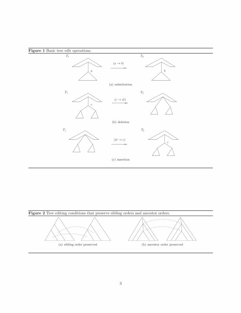
Figure 1 Basic tree edit operations.

(a→ b)

a b

T2T1

(a) substitution

T2

(c→ ∅)

c

T1

(b) deletion

T1

(∅→ c)c

T2

(c) insertion

Figure 2 Tree editing conditions that preserve sibling orders and ancestor orders.

(a) sibling order preserved (b) ancestor order preserved

3

case, that if we know the solutions of some subproblems each of which being a modification from the originalproblem by one of the three aforementioned basic operations, then the solution of the original problem can beconstructed from the solutions of these subproblems by means of a finite number of simple arithmetics. Thesame principle holds recursively for all the subproblems. The tree-to-tree distance d(T, T ′) in Equation 2 iscomputed as in Equation 3. Meanwhile, when both forests are composed of one tree (i.e., (F,G) = (T, T ′)),Equation 2 reduces to Equation 3 which in turn makes use of Equation 2 for computing the associatedsubforest distances.

d(T, T ′) = min

d(T − r(T ), T ′) + δ(r(T ),∅),d(T, T ′ − r(T ′)) + δ(∅, r(T ′)),d(T − r(T ), T ′ − r(T ′)) + δ(r(T ), r(T ′))

. (3)

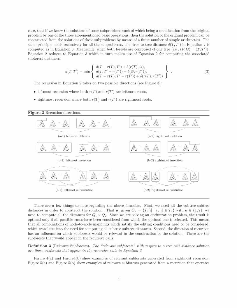
The recursion in Equation 2 takes on two possible directions (see Figure 3):

• leftmost recursion where both r(T ) and r(T ′) are leftmost roots,

• rightmost recursion where both r(T ) and r(T ′) are rightmost roots.

Figure 3 Recursion directions.

...

...

(a-1) leftmost deletion

...

...

(a-2) rightmost deletion

...

...

(b-1) leftmost insertion

...

...

(b-2) rightmost insertion

...

...

(c-1) leftmost substitution

...

...

(c-2) rightmost substitution

There are a few things to note regarding the above formulae. First, we need all the subtree-subtreedistances in order to construct the solution. That is, given Qa = Ta[i] | ta[i] ∈ Ta with a ∈ 1, 2, weneed to compute all the distances for Q1 ×Q2. Since we are solving an optimization problem, the result isoptimal only if all possible cases have been considered from which the optimal one is selected. This meansthat all combinations of node-to-node mappings which satisfy the editing conditions need to be considered,which translates into the need for computing all subtree-subtree distances. Second, the direction of recursionhas an influence on which subforests would be relevant in the construction of the solution. These are thesubforests that would appear in the recursive calls.

Definition 3 (Relevant Subforests). The “relevant subforests” with respect to a tree edit distance solutionare those subforests that appear in the recursive calls in Equation 2.

Figure 4(a) and Figure4(b) show examples of relevant subforests generated from rightmost recursion.Figure 5(a) and Figure 5(b) show examples of relevant subforests generated from a recursion that operates

4

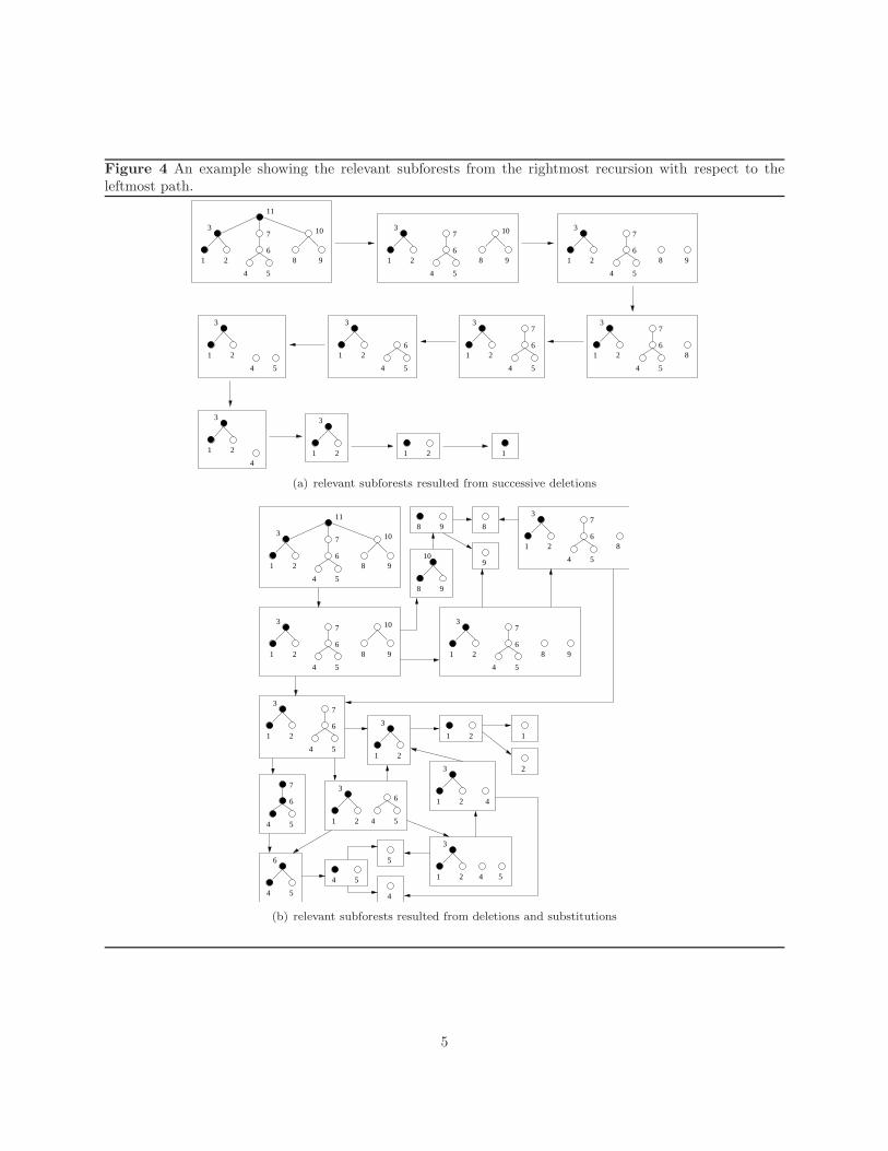
Figure 4 An example showing the relevant subforests from the rightmost recursion with respect to theleftmost path.

2 1

1 2

3

4 5

6

7

8 9

10

11

1 2

3

4 5

6

7

8 9

10

1 2

3

4 5

6

7

8 9

1 2

3

4 5

1 2

3

4 5

61 2

3

4 5

6

7

1 2

3

4 5

6

7

8

1 2

3

41 2

3

1

(a) relevant subforests resulted from successive deletions

1 2

3

4 5

6

7

8 9

10

11

1 2

3

4 5

6

7

8 9

10

8 9

10

8

9

1 2

3

4 5

6

7

1 2

3

4 5

6

7

8

4 5

6

7

4 5

6

1 2

3

4 5

5

4 5

1 2

3

4 5

6

7

8 9

8 9

1 2

3

4

1 2

3

4 5

6

1 2

3

1 2

2

1

4

(b) relevant subforests resulted from deletions and substitutions

5

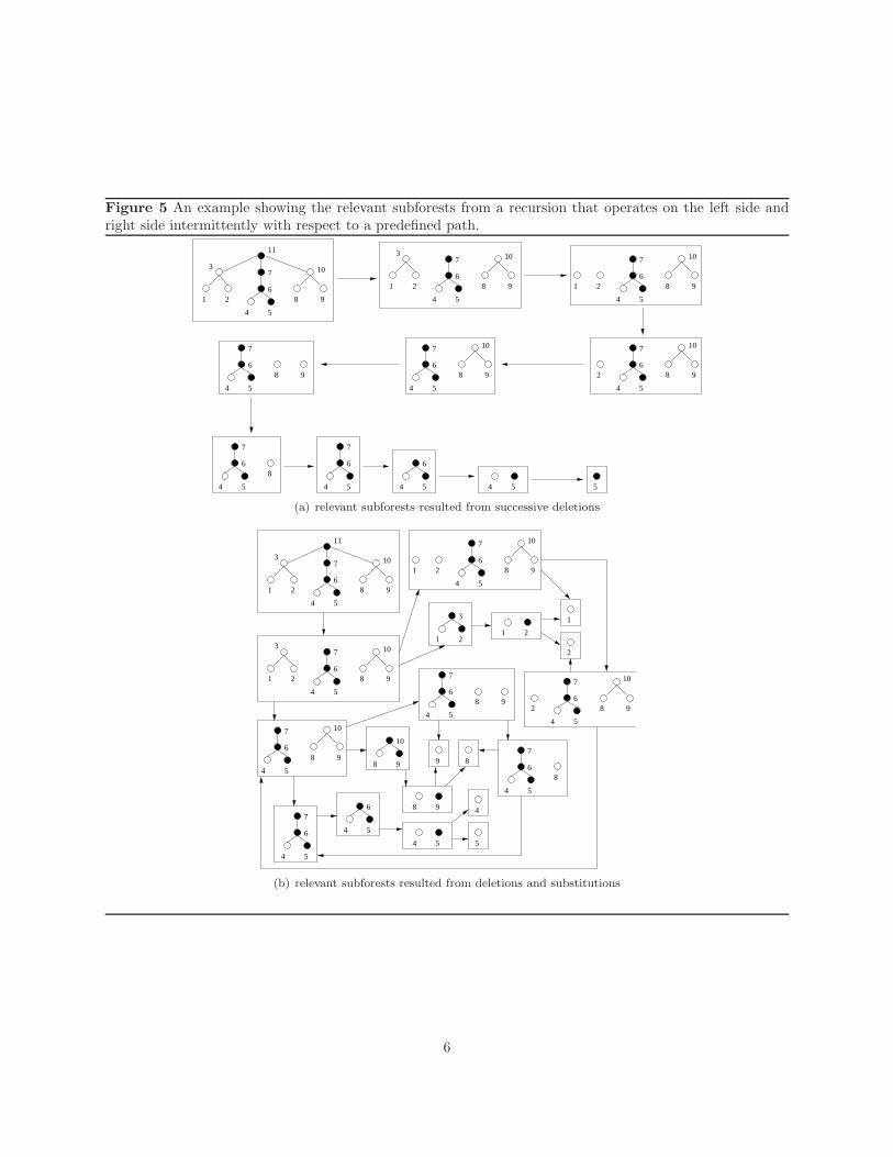
Figure 5 An example showing the relevant subforests from a recursion that operates on the left side andright side intermittently with respect to a predefined path.

5 5

1 2

3

4 5

6

7

8 9

10

11

1 2

3

4 5

6

7

8 9

10

1 2

4 5

6

7

8 9

10

4 5

6

7

8 9

4 5

6

7

8 9

10

2

4 5

6

7

8 9

10

4 5

6

7

8

4 5

6

7

4 5

6

4

(a) relevant subforests resulted from successive deletions

1 2

3

4 5

6

7

8 9

10

11

1 2

3

1 2

3

4 5

6

7

8 9

10

4 5

8 9

10

4 5

6

7

8 9

10

4 5

6

7

8 9

1 2

8 9

9

4 5

6 4

5

1 2

4 5

6

7

8 9

10

8

4 5

6

7

8

4 5

6

7

2

4 5

6

7

8 9

10

1

2

(b) relevant subforests resulted from deletions and substitutions

6

on the left side and right side intermittently with respect to a predefined path. More details will be given inthe next section regarding this type of recursion.

In constructing an algorithmic solution based on Equation 2, there are two complementary aspects toconsider:

• Top-down aspect: This concerns the direction from the left-hand side to the right-hand side of therecursion.

• Bottom-up aspect: This concerns the direction from the right-hand side to the left-hand side of therecursion.

In the context of complexity analysis, we express the number of elementary operations in terms of thenumber of recursive calls along relevant recursion paths or the number of steps in a bottom-up enumerationsequence, interchangeably. This is due to the fact that to every sequence of top-down recursive calls basedon Equation 2 corresponds a sequence of bottom-up enumeration steps.

Our plan in understanding the complexity issues is to start with the bottom-up aspect and eventuallyrelate it to the top-down aspect. As such, we initially consider procedures based on the bottom-up style. Asa starting point, consider the following approaches:

• the recursion direction is fixed to be either leftmost or rightmost,

• the recursion direction may vary between leftmost and rightmost.

In either approach, we need an enumeration scheme which specifies the order of distance computationsfor the subproblems.

Fixed-Direction Recursion: For recursion of fixed direction, a naive scheme is to arrange the subtree-subtree distance computations, as well as the relevant forest-forest distance computations, in one of twoalternative ways as follows:

• LR-postorder: The subtrees as well as the subforests contained in each subtree are enumerated inleft-to-right postorder.

• RL-postorder: The subtrees as well as the subforests contained in each subtree are enumerated inright-to-left postorder.

The procedures for sorting the enumeration order for subforests are listed in Algorithms 1 and 2.

Algorithm 1: Construct an enumeration scheme for the subforests of a tree T based on LR-postorder.

input : T , with |T | = noutput: an enumeration sequence L of subforests of T based on the LR-postorder

label the nodes of T in LR-postorder ;1

for i← 1 to n do2

construct Si to be a sequence of subforests of T [i] with the rightmost root enumerated in3

LR-postorder ;

L = S1 ;4

for i← 2 to n do5

L = L Si ;6

output L ;7

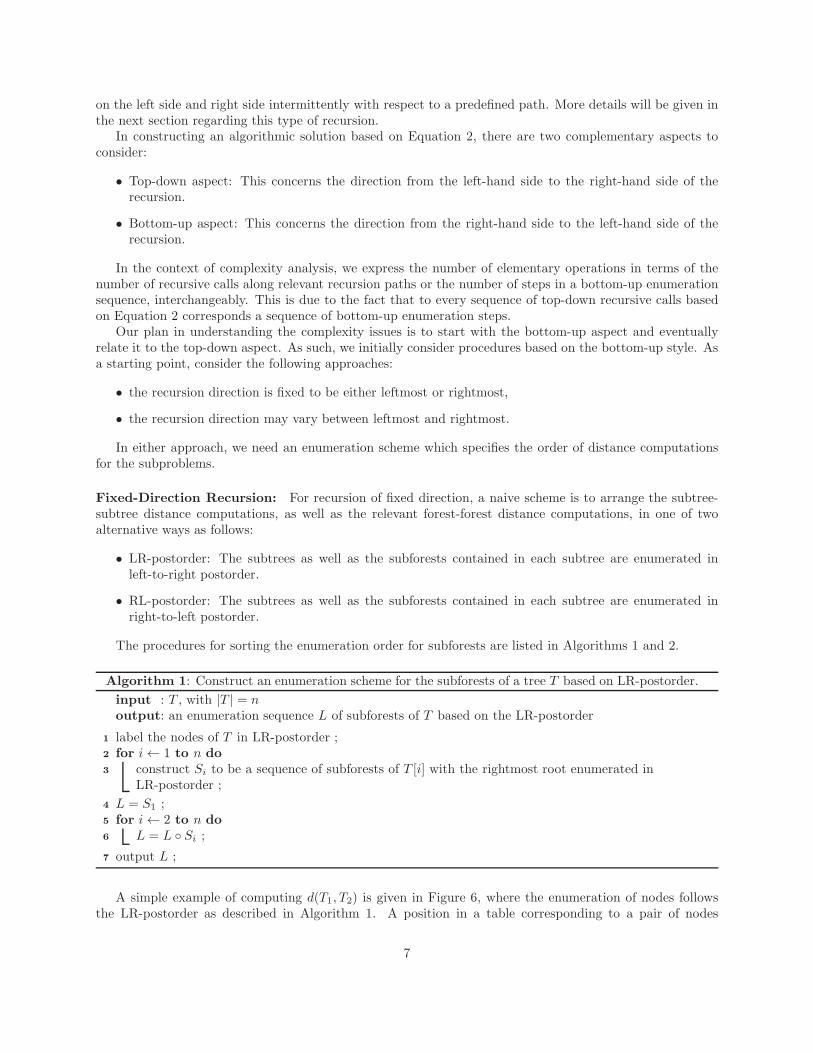
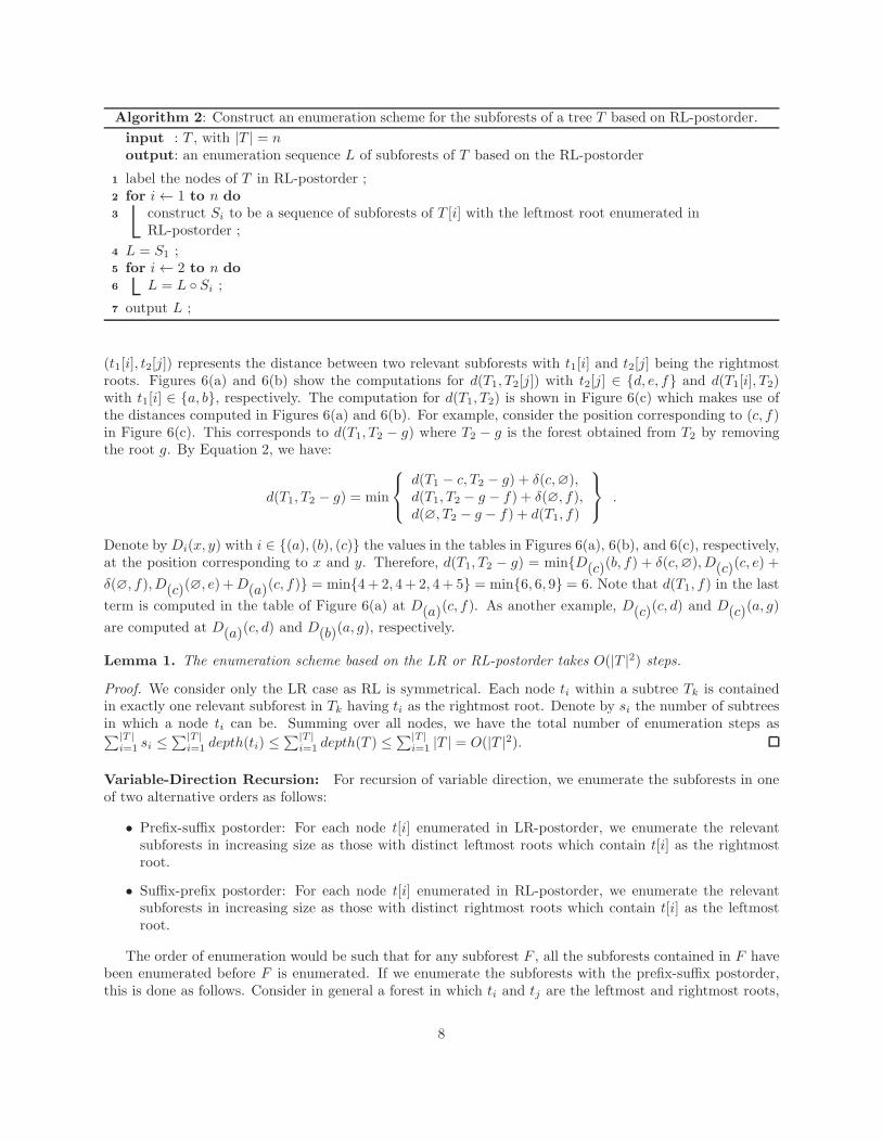
A simple example of computing d(T1, T2) is given in Figure 6, where the enumeration of nodes followsthe LR-postorder as described in Algorithm 1. A position in a table corresponding to a pair of nodes

7

Algorithm 2: Construct an enumeration scheme for the subforests of a tree T based on RL-postorder.

input : T , with |T | = noutput: an enumeration sequence L of subforests of T based on the RL-postorder

label the nodes of T in RL-postorder ;1

for i← 1 to n do2

construct Si to be a sequence of subforests of T [i] with the leftmost root enumerated in3

RL-postorder ;

L = S1 ;4

for i← 2 to n do5

L = L Si ;6

output L ;7

(t1[i], t2[j]) represents the distance between two relevant subforests with t1[i] and t2[j] being the rightmostroots. Figures 6(a) and 6(b) show the computations for d(T1, T2[j]) with t2[j] ∈ d, e, f and d(T1[i], T2)with t1[i] ∈ a, b, respectively. The computation for d(T1, T2) is shown in Figure 6(c) which makes use ofthe distances computed in Figures 6(a) and 6(b). For example, consider the position corresponding to (c, f)in Figure 6(c). This corresponds to d(T1, T2 − g) where T2 − g is the forest obtained from T2 by removingthe root g. By Equation 2, we have:

d(T1, T2 − g) = min

d(T1 − c, T2 − g) + δ(c,∅),d(T1, T2 − g − f) + δ(∅, f),d(∅, T2 − g − f) + d(T1, f)

.

Denote by Di(x, y) with i ∈ (a), (b), (c) the values in the tables in Figures 6(a), 6(b), and 6(c), respectively,at the position corresponding to x and y. Therefore, d(T1, T2 − g) = minD(c)(b, f) + δ(c,∅), D(c)(c, e) +

δ(∅, f), D(c)(∅, e) +D(a)(c, f) = min4+ 2, 4+ 2, 4+ 5 = min6, 6, 9 = 6. Note that d(T1, f) in the last

term is computed in the table of Figure 6(a) at D(a)(c, f). As another example, D(c)(c, d) and D(c)(a, g)

are computed at D(a)(c, d) and D(b)(a, g), respectively.

Lemma 1. The enumeration scheme based on the LR or RL-postorder takes O(|T |2) steps.

Proof. We consider only the LR case as RL is symmetrical. Each node ti within a subtree Tk is containedin exactly one relevant subforest in Tk having ti as the rightmost root. Denote by si the number of subtreesin which a node ti can be. Summing over all nodes, we have the total number of enumeration steps as∑|T |

i=1 si ≤∑|T |

i=1 depth(ti) ≤∑|T |

i=1 depth(T ) ≤∑|T |

i=1 |T | = O(|T |2).

Variable-Direction Recursion: For recursion of variable direction, we enumerate the subforests in oneof two alternative orders as follows:

• Prefix-suffix postorder: For each node t[i] enumerated in LR-postorder, we enumerate the relevantsubforests in increasing size as those with distinct leftmost roots which contain t[i] as the rightmostroot.

• Suffix-prefix postorder: For each node t[i] enumerated in RL-postorder, we enumerate the relevantsubforests in increasing size as those with distinct rightmost roots which contain t[i] as the leftmostroot.

The order of enumeration would be such that for any subforest F , all the subforests contained in F havebeen enumerated before F is enumerated. If we enumerate the subforests with the prefix-suffix postorder,this is done as follows. Consider in general a forest in which ti and tj are the leftmost and rightmost roots,

8

Figure 6 Tables for the computation of d(T1, T2). The basic edit costs are defined as follows: δ(x, y) = 1if x 6= y, and 0 if x = y. δ(x,∅) = δ(∅, x) = 2. The optimal edit scripts can be traced with the arrowsequences.

ba

c

T1

e

g

fdT2

∅ d, e, f∅ 0 2

↑ տa 2 1↑ տ ↑

b 4 3տ ↑

c 6 5(a)

∅ d e f g∅ 0 ← 2 ← 4 ← 6 8

տ տ տ տa, b 2 1 ← 3 ← 5 ← 7

(b)

∅ d e f g∅ 0 ← 2 4 6 8

տ տa 2 1 ← 3 5 7

տ տb 4 3 2 ← 4 6

տc 6 5 4 6 5

(c)

9

respectively. The rightmost root is enumerated in a left-to-right postorder starting at the leftmost leaf.For each tj thus enumerated, consider the largest forest with tj being the rightmost root. Now, to obtainthe order for the subforests contained in this forest with tj being the rightmost root, let F1, F2, · · · , Fk bethe sequence of subforests resulted from successively deleting the leftmost root from the forest until onlythe rightmost subtree rooted on tj remains, i.e., Fk = T [tj ]. The order we want is the reverse sequenceFk, Fk−1, · · · , F1. In this way, we obtain a sequence of subforests for each tj . Concatenate all the sequencesin the increasing order of tj , we have the final sequence of all the subforests of T arranged in a properorder. The alternative way of enumerating the subforests, namely the suffix-prefix postorder, is handledsymmetrically. The procedures are listed in Algorithms 3 and 4.

Algorithm 3: Construct an enumeration scheme for the subforests of a tree T based on prefix-suffixpostorder.

input : T , with |T | = noutput: an enumeration sequence L of subforests of T based on the prefix-suffix postorder

construct P to be a sequence of subforests of T resulted from successive deletion on the rightmost1

root ; /* P [1] = T */

construct P ′ = (F1, F2, · · · , Fn) to be the reverse sequence of P ; /* Fn = T */2

for i← 1 to n do3

construct Si to be a sequence of subforests of Fi ∈ P ′, all sharing the same rightmost root,4

resulted from successive deletion on the leftmost root ; /* Si[1] = Fi,

Si[k] = Si[k − 1]− lm root(Si[k − 1]), rm root(Si[k]) = rm root(Si[k − 1]), ∀k > 1 */

construct S′i to be the reverse sequence of Si ; /* S′

i[|S′i|] = Fi */5

L = S′1 ;6

for i← 2 to n do /* concatenate all sequences */7

L = L S′i ;8

output L ;9

Algorithm 4: Construct an enumeration scheme for the subforests of a tree T based on suffix-prefixpostorder.

input : T , with |T | = noutput: an enumeration sequence L of subforests of T based on the suffix-prefix postorder

construct S to be a sequence of subforests of T resulted from successive deletion on the leftmost root ;1

/* S[1] = T */

construct S′ = (F1, F2, · · · , Fn) to be the reverse sequence of S ; /* Fn = T */2

for i← 1 to n do3

construct Pi to be a sequence of subforests of Fi ∈ S′, all sharing the same leftmost root, resulted4

from successive deletion on the rightmost root ; /* Pi[1] = Fi,

Pi[k] = Pi[k − 1]− rm root(Pi[k − 1]), lm root(Pi[k]) = lm root(Pi[k − 1]), ∀k > 1 */

construct P ′i to be the reverse sequence of Pi ; /* P ′

i [|P′i |] = Fi */5

L = P ′1 ;6

for i← 2 to n do /* concatenate all sequences */7

L = L P ′i ;8

output L ;9

Examples of prefix-suffix and suffix-prefix postorder enumerations are given in Figure 7 and Figure 8,respectively. In Figure 7, subforests having the same rightmost root are in contiguous boxes, whereas inFigure 8, subforests having the same leftmost root are in contiguous boxes.

10

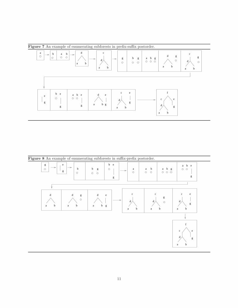
Figure 7 An example of enumerating subforests in prefix-suffix postorder.

a b a b

a b

d

a b

d

c

g

a b

d

cgb g a b g

a b

d g

e

g

b e

g

a b

g

e

a b g

ed

a b

d

c e

g

a b

d

c

f

e

g

Figure 8 An example of enumerating subforests in suffix-prefix postorder.

g e

gb b g

b e

g

a a b a b ga b

g

e

a b

d

g

e

a b

d

a b

d g

a b

d

c e

g

a b

d

c

a b

d

cg

a b

d

c

f

e

g

11

Lemma 2. The enumeration scheme based on prefix-suffix or suffix-prefix postorder takes O(|T |2) steps.

Proof. We consider only the prefix-suffix postorder as the suffix-prefix postorder is the symmetrical case.Denote by fi the number of subforests with distinct leftmost roots which contain ti as the rightmost root.

Summing over all nodes, we have∑|T |

i=1 fi ≤∑|T |

i=1 |T | = O(|T |2).

An algorithm for computing tree edit distances where the relevant subforests are enumerated by theabove procedures is given in Algorithm 5. The algorithm can be implemented using O(|T1| × |T2|) space ifthe forest distances are allowed to be overwritten.

Algorithm 5: Compute tree edit distance in O(m2n2) time.

input : (T1, T2), with |T1| = m and |T2| = noutput: d(T1[i], T2[j]) for 1 ≤ i ≤ m and 1 ≤ j ≤ n

sort relevant subforests of (T1, T2) into (L1, L2) as in Algorithms 1, 2, 3, or 4 ;1

for i← 1 to |L1| do2

for j ← 1 to |L2| do3

compute d(L1[i], L2[j]) as in Equation 2 ;4

Theorem 1. The tree edit distance as computed in Algorithm 5 takes O(m2n2) time, where m = |T1|, andn = |T2|.

Proof. The result follows directly from Lemma 1 and 2.

The algorithms presented in this section follow a bottom-up dynamic programming style where the treenodes are numbered in postorder, in contrast to the preorder numbering of nodes in Tai’s algorithm [11].The way Tai’s algorithm works is to progressively increase the sizes of the trees, by one node at a timefollowing the preorder numbers, and compute the distance for each such pair of partial trees1.

3 Improved Algorithmic Strategies

The algorithm presented in the previous section is based on the principle of dynamic programming whichrelies on a well-defined scheme for enumerating the relevant subforests. In this approach, forest distances arearranged in a certain order so as to facilitate the relay of distance computations. Essentially, we take advan-tage of the overlap among subforests that are contained in the same subtree. To make further improvement,we look for ways to take advantage of the overlap among subtrees as well.

3.1 Leftmost Paths

We examine recursion of fixed direction, say rightmost recursion, the situation for leftmost recursion beingsymmetrical. This means that the enumeration will be in LR-postorder. Consider a path (t1, t2, · · · , tk)where ti is the leftmost child of ti+1 for 1 ≤ i ≤ k−1. Let (T1, T2, · · · , Tk) be the sequence of subtrees whereti is the root of Ti, and (F1, F2, · · · , Fk) be the sequence of sets where Fi denotes the set of subforests of Ti

all containing the leftmost leaf of Ti. We have F1 ⊂ F2 ⊂ · · · ⊂ Fk. This means that enumerating Fk onceeffectively takes care of the enumerations for F1, F2, · · · , Fk−1. To generalize this situation to the whole tree,we see that all subtrees sharing the same leftmost leaf can be handled together. Carried out in this way,a tree is recursively decomposed into disjoint leftmost paths where each such leftmost path is shared by aset of subtrees which can be handled together along this path with the LR-postorder enumeration thereby

1In fact, it does not compute the true distance since it only considers the optimal mappings along a pair of paths for each pairof partial trees, instead of the entire partial trees. If Algorithm 5 is applied for each pair of partial trees, the time complexityis easily seen as O(m3n3).

12

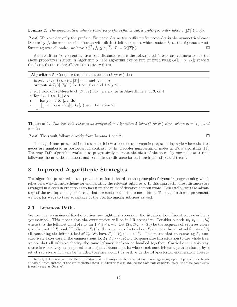
removing the repetitions. This strategy was developed by Zhang and Shasha [13]. An example of such pathdecomposition is given in Figure 9(a).

Figure 9 Leftmost paths and rightmost paths (in thick edges).

(a) leftmost paths (b) rightmost paths

Each leftmost path corresponds to the smallest subtree that contains this path, and the root of thissubtree is referred to as an “LR-keyroot”, which is defined as follows.

Definition 4 (LR-keyroots). An LR-keyroot is either the root of T or has a left sibling.

The new enumeration scheme works as follows. We identify all the LR-keyroots in the tree, and sortthem in increasing order by their LR-postorder numbers, referred to as “LR-keyroot postorder”. This willbe the order by which the subforests are enumerated, i.e., based on the LR-keyroots with which they areassociated. The procedure is listed in Algorithm 6.

Algorithm 6: Construct the enumeration scheme for the subforests of a tree T in LR-keyroot postorder.The RL-based procedure is symmetrical to this.

input : T , with |T | = noutput: an enumeration sequence L of subforests of T in the LR-keyroot postorder

identify the LR-keyroots of T ;1

sort the LR-keyroots in increasing order of LR-postorder numbers into a list K = k1, k2, · · · , kl ;2

for i← 1 to l do3

construct Si to be a sequence of subforests of T [ki] with the rightmost root enumerated in4

LR-postorder ;

L = S1 ;5

for i← 2 to n do6

L = L Si ;7

output L ;8

This enumeration scheme gives rise to the algorithm in Algorithm 7.

Algorithm 7: Compute tree edit distance in O(mn∏2

i=1 mindepth(Ti),#leaves(Ti)) time.

input : (T1, T2), with |T1| = m and |T2| = noutput: d(T1[i], T2[j]) for 1 ≤ i ≤ m and 1 ≤ j ≤ n

sort relevant subforests of (T1, T2) into (L1, L2) as in Algorithm 6 ;1

for i← 1 to |L1| do2

for j ← 1 to |L2| do3

compute d(L1[i], L2[j]) as in Equation 2 ;4

13

Theorem 2. The algorithm computes d(T1[i], T2[j]) for all 1 ≤ i ≤ |T1| and 1 ≤ j ≤ |T2|.

Proof. We prove it by induction on the sizes of the subtrees induced by the keyroots.Base case: This involves only the singleton subtrees. Since all the basic edit costs with respect to singlenodes are already defined, the base case holds.Induction hypothesis: For any (i, j) ∈ (i, j) | i ∈ LR-keyroots(T1), j ∈ LR-keyroots(T2), just before thecomputation of d(T1[i], T2[j]), the following set of distances have been computed, D = D1 ∪D2 where

• D1 = d(T1[i′], T2[j

′]) | i′ ∈ T1[i]− leftmost-path(T1[i]), j′ ∈ T2[j],

• D2 = d(T1[i′], T2[j

′]) | i′ ∈ T1[i], j′ ∈ T2[j]− leftmost-path(T2[j]).

Induction step: We show that d(T1[i′], T2[j

′]) | i′ ∈ T1[i], j′ ∈ T2[j] are all computed. The subtree-subtree distances to be computed in the process of computing d(T1[i], T2[j]) are d(T1[i

′], T2[j′]) | i′ ∈

leftmost-path(T1[i]), j′ ∈ leftmost-path(T2[j]). The induction step holds since it is in accord with theLR-keyroot postorder that the algorithm follows, which means that all distances specified in the inductionhypothesis have been computed. This concludes the proof.

To see the impact of the leftmost-path decomposition scheme on the time complexity, it is necessary tointroduce the concept of “LR-collapsed depth” defined as follows.

Definition 5 (LR-Collapsed Depth). The LR-collapsed depth of a node ti is the number of its ances-tors that are LR-keyroots. The LR-collapsed depth of a tree T is defined as LR-collapsed-depth(T ) =max LR-collapsed-depth(ti) | ti ∈ T .

Intuitively, the LR-collapsed depth of a tree T represents the maximal number of non-leaf LR-keyrootsthat a path in T may contain. We define LR-collapsed depth as a way to estimate the maximal times a node,representing the rightmost root of some relevant subforest, is enumerated with the LR-keyroot postorder.As a consequence of this enumeration scheme, repetitious enumerations involving a given node are removedsince subtrees containing this node as well as having the same leftmost leaf are no longer handled separately.

Lemma 3. LR-collapsed-depth(T ) ≤ min depth(T ),#leaves(T ).

Proof. Since the number of LR-keyroots on any path is bounded by the depth of the path, we haveLR-collapsed-depth(T ) ≤ depth(T ). For any two LR-keyroots ki and kj , the subtrees Ti and Tj rootedat ki and kj have distinct leftmost leaves. This means that the number of subtrees in T that are rootedat LR-keyroots can not exceed the number of leaves, i.e., #LR-keyroots(T ) ≤ #leaves(T ). Since thenumber of LR-keyroots on any path is no more than the total number of LR-keyroots in the tree, i.e.,LR-collapsed-depth(T ) ≤ #LR-keyroots(T ), we have LR-collapsed-depth(T ) ≤ #leaves(T ). Therefore,LR-collapsed-depth(T ) can be bounded by depth(T ) or #leaves(T ), whichever is smaller. This concludesthe proof.

Here is the implication of Lemma 3. In the previous procedure, a node in T may be enumerateddepth(T ) times with the LR-postorder enumeration scheme, because the maximal number of subtrees inwhich a node may be contained is depth(T ). Grouping together subtrees with the same leftmost leaf canremove the repetitions, and the improvement is evident since the upper bound is reduced from depth(T ) tomin depth(T ),#leaves(T ).

Theorem 3. The tree edit distance problem can be solved in O(mn∏2

i=1 mindepth(Ti),#leaves(Ti)) time,where m = |T1| and n = |T2|.

Proof. From Lemma 3, each node, representing the rightmost root of some relevant subforest, in T is enu-merated at most LR-collapsed-depth(T ) times using the enumeration scheme in Algorithm 6. Hence, theresult follows directly.

Theorem 4. The tree edit distance problem can be solved in O(mn) space, where m = |T1| and n = |T2|.

14

Proof. The computation uses two m× n tables Dt and Df . The forest-forest distances are computed in Df

where the values can be overwritten when the computation moves from one pair of subtrees to another pair.The subtree-subtree distances obtained in the process of computing the forest-forest distances are stored inDt, and fetched for use in computing forest-forest distances.

In this section, a new way is presented for enumerating the relevant subforests in LR-postorder whererepetitious steps associated with the leftmost paths in a tree are eliminated, resulting in an improved timecomplexity. However, depending on the shapes of the trees, the leftmost-path decomposition for some treeshapes could yield marginal benefits regarding the running time. This leads to the strategy to be presentedin the next section.

3.2 Heavy Paths on One Tree

We see from the previous section that the computation time is due to the enumeration of subforests whereeach enumeration step counts a constant time in performing a few simple arithmetics. The leftmost-pathstrategy improves the time complexity by enumerating subtrees with overlapping leftmost paths together inthe same sequence of computation. Since the running time is dependent on the shapes of the trees, it isworthwhile to consider a different type of path decomposition that can also offer benefits with respect tothe complexity. This possibility was explored and a new decomposition strategy based on a type of pathreferred to as “heavy path” is due to Klein [7]. In contrast to the Zhang-Shasha strategy, which may beseen as a way of improving upon the naive fixed-direction procedure based on the LR-postorder enumerationscheme given in Section 2, the new strategy may be seen as a way of improving upon the variable-directionprocedure based on the prefix-suffix or suffix-prefix postorder enumeration scheme. We give a few definitionsrelated to the idea behind heavy path.

Definition 6 (Heavy Child/Node). For any node t in T , the child th which is the root of the largest subtree(breaking tie arbitrarily) among the sibling subtrees is the heavy child of t. We use the terms “heavy child”and “heavy node” interchangeably.

The definition of heavy path is given as follows.

Definition 7 (Heavy Path). [10, 6] The heavy path of a tree T is a unique path connecting the root and aleaf of T on which every node, except the root, is a heavy node.

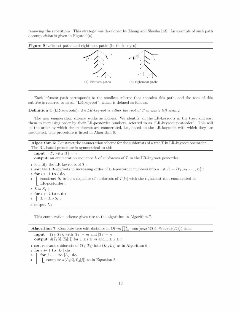
Figure 10 shows an example of a tree recursively decomposed into a set of heavy paths.

Figure 10 Heavy paths (in thick edges).

Similar to LR and RL-postorder which are defined with respect to the leftmost path and rightmost path,respectively, we define an enumeration scheme with respect to the heavy path as follows.

Definition 8 (H-Postorder). The nodes in tree T is enumerated in H-postorder as follows. Start at the leaftl on heavy-path(T ), enumerate the subtrees rooted on its right siblings, if any, in LR postorder, then thesubtrees rooted on its left siblings, if any, in RL postorder. Continue and repeat the same process with eachnext higher node on heavy-path(T ) until reaching root(T ).

15

If we ignore what happens on the left side of the heavy-path during an H-postorder enumeration, then wesee a sequence of enumeration steps identical to an LR-postorder enumeration. If we ignore what happens onthe right side of the heavy-path during an H-postorder enumeration, then we see a sequence of enumerationsteps identical to an RL-postorder enumeration. Alternatively, a second version symmetrical to this one, i.e.,RL then LR intermittently, also works. In the following presentation, the version in Definition 8 is used. Anexample of enumerating subforests in H-postorder is given in Figure 11.

Figure 11 An example of enumerating subforests in H-postorder.

a g

a

b

d

c

b

a

b

c

d

g

ec

b

a

b

c

d

a

b

c

d e

f

g

c

b

Analogous to LR-keyroots, a type of keyroots specific to this context is defined as follows.

Definition 9 (H-keyroots). An H-keyroot is either the root of T or the root of a subtree in T that has alarger sibling subtree. If multiple subtrees are equally the largest among their sibling subtrees, all but one(chosen arbitrarily) are H-keyroots.

Definitions 6 and 9 are equivalent since for any node, once its heavy child is specified, the other childrenare H-keyroots, and vice versa. A node in a tree is either a heavy node or an H-keyroot.

The algorithm works as follows. The H-keyroots in the larger tree are sorted into a list L1 in increasing H-postorder numbers. For each subtree of which the root is in L1, order the relevant subforests in H-postorder,and concatenate all the ordered sequences to form the entire sequence as listed in Algorithm 8, which wecall the “H-keyroot postorder”. On the smaller tree, all subforests are ordered into a list L2 in prefix-suffixor suffix-prefix postorder, as in Algorithms 3 or 4. The new algorithm is listed in Algorithm 9.

Algorithm 8: Construct the enumeration scheme for the subforests of a tree T in H-keyroot postorder.

input : T , with |T | = noutput: an enumeration sequence L of subforests of T in the H-keyroot postorder

identify the H-keyroots of T ;1

sort the H-keyroots in increasing order of H-postorder numbers into a list K = k1, k2, · · · , kl ;2

for i← 1 to l do3

construct Si to be a sequence of subforests of T [ki] enumerated in H-postorder ;4

L = S1 ;5

for i← 2 to n do6

L = L Si ;7

output L ;8

Theorem 5. The algorithm computes d(T1[i], T2[j]) for all 1 ≤ i ≤ |T1| and 1 ≤ j ≤ |T2|.

Proof. We prove it by induction on the sizes of the subtrees induced by the keyroots.Base case: This involves only the singleton subtrees. Since all the basic edit costs with respect to singlenodes are already defined, the base case holds.Induction hypothesis: For any k ∈ k | k ∈ H-keyroots(T2), just before the computation of d(T1, T2[k]),d(T1[i], T2[j]) | i ∈ T1, j ∈ T2[k]− heavy-path(T2[k]) have been computed.

16

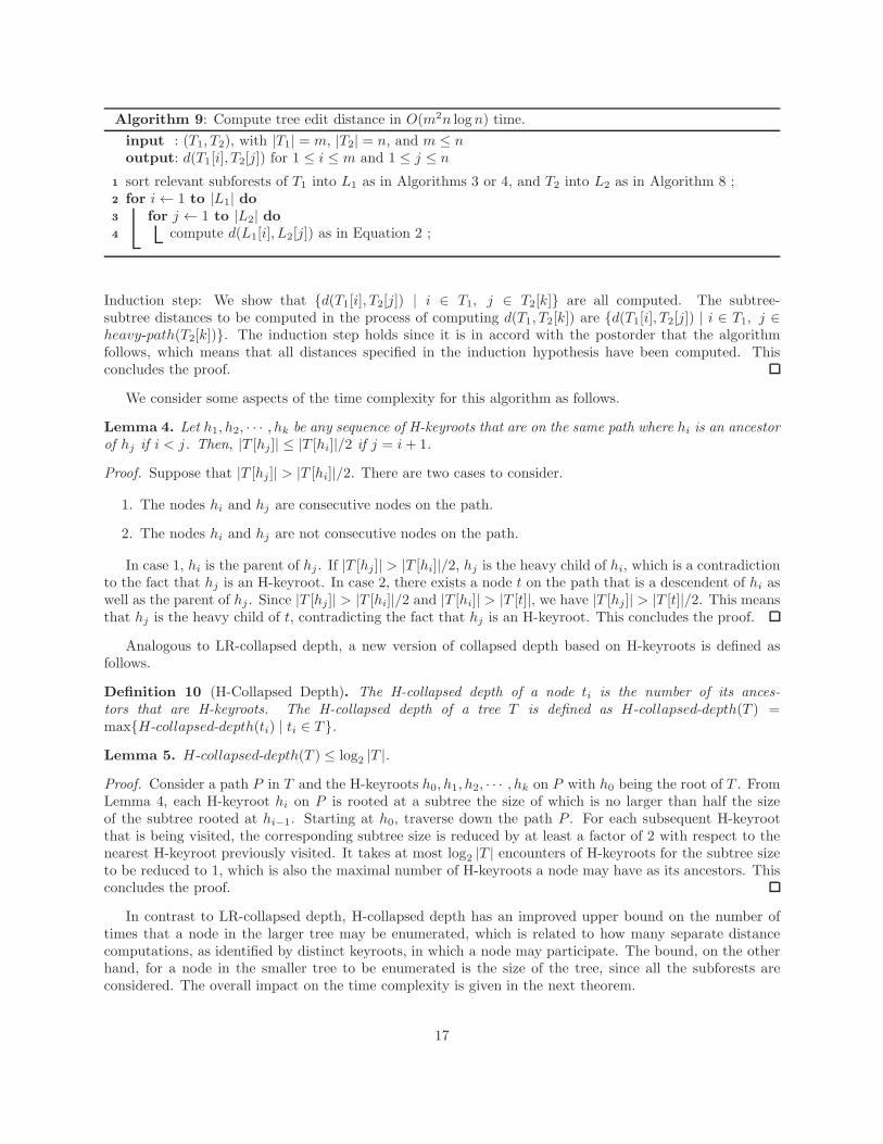
Algorithm 9: Compute tree edit distance in O(m2n logn) time.

input : (T1, T2), with |T1| = m, |T2| = n, and m ≤ noutput: d(T1[i], T2[j]) for 1 ≤ i ≤ m and 1 ≤ j ≤ n

sort relevant subforests of T1 into L1 as in Algorithms 3 or 4, and T2 into L2 as in Algorithm 8 ;1

for i← 1 to |L1| do2

for j ← 1 to |L2| do3

compute d(L1[i], L2[j]) as in Equation 2 ;4

Induction step: We show that d(T1[i], T2[j]) | i ∈ T1, j ∈ T2[k] are all computed. The subtree-subtree distances to be computed in the process of computing d(T1, T2[k]) are d(T1[i], T2[j]) | i ∈ T1, j ∈heavy-path(T2[k]). The induction step holds since it is in accord with the postorder that the algorithmfollows, which means that all distances specified in the induction hypothesis have been computed. Thisconcludes the proof.

We consider some aspects of the time complexity for this algorithm as follows.

Lemma 4. Let h1, h2, · · · , hk be any sequence of H-keyroots that are on the same path where hi is an ancestorof hj if i < j. Then, |T [hj]| ≤ |T [hi]|/2 if j = i+ 1.

Proof. Suppose that |T [hj]| > |T [hi]|/2. There are two cases to consider.

1. The nodes hi and hj are consecutive nodes on the path.

2. The nodes hi and hj are not consecutive nodes on the path.

In case 1, hi is the parent of hj . If |T [hj]| > |T [hi]|/2, hj is the heavy child of hi, which is a contradictionto the fact that hj is an H-keyroot. In case 2, there exists a node t on the path that is a descendent of hi aswell as the parent of hj . Since |T [hj]| > |T [hi]|/2 and |T [hi]| > |T [t]|, we have |T [hj]| > |T [t]|/2. This meansthat hj is the heavy child of t, contradicting the fact that hj is an H-keyroot. This concludes the proof.

Analogous to LR-collapsed depth, a new version of collapsed depth based on H-keyroots is defined asfollows.

Definition 10 (H-Collapsed Depth). The H-collapsed depth of a node ti is the number of its ances-tors that are H-keyroots. The H-collapsed depth of a tree T is defined as H-collapsed-depth(T ) =maxH-collapsed-depth(ti) | ti ∈ T .

Lemma 5. H-collapsed-depth(T ) ≤ log2 |T |.

Proof. Consider a path P in T and the H-keyroots h0, h1, h2, · · · , hk on P with h0 being the root of T . FromLemma 4, each H-keyroot hi on P is rooted at a subtree the size of which is no larger than half the sizeof the subtree rooted at hi−1. Starting at h0, traverse down the path P . For each subsequent H-keyrootthat is being visited, the corresponding subtree size is reduced by at least a factor of 2 with respect to thenearest H-keyroot previously visited. It takes at most log2 |T | encounters of H-keyroots for the subtree sizeto be reduced to 1, which is also the maximal number of H-keyroots a node may have as its ancestors. Thisconcludes the proof.

In contrast to LR-collapsed depth, H-collapsed depth has an improved upper bound on the number oftimes that a node in the larger tree may be enumerated, which is related to how many separate distancecomputations, as identified by distinct keyroots, in which a node may participate. The bound, on the otherhand, for a node in the smaller tree to be enumerated is the size of the tree, since all the subforests areconsidered. The overall impact on the time complexity is given in the next theorem.

17

Theorem 6. The tree edit distance problem can be solved in O(m2n logn) time where |T1| = m, |T2| = n,and m ≤ n.

Proof. For any (i, j) with i ∈ T1 and j ∈ T2, i is enumerated the number of times equal the number ofsubforests with distinct leftmost roots which contain i as the rightmost root, or alternatively, the number ofsubforests with distinct rightmost roots which contain i as the leftmost root. This is bounded by the size ofT1, i.e., m. On the other hand, j is enumerated at most 1 + log2 n times according to Lemma 5, since thisis the upper bound on the number of subtrees in T2 rooted on distinct H-keyroots which contain j, and ineach one j is enumerated once. The result thus follows.

Theorem 7. The new algorithm solves the tree edit distance problem in O(mn) space where |T1| = m,|T2| = n, and m ≤ n.

Proof. We use a 2 × m2 table where the m2 subforests in T1 are arranged in prefix-suffix or suffix-prefixorder. For T2, the idea is essentially a linear-space algorithm by which distances for only one subforest arecomputed and updated when moving to the next subforest in the enumeration sequence. The subtree-subtreedistances are stored in an m× n table.

In the next section, we see how this algorithm is improved by a strategy that finds a way to applyheavy-path decompositions on both trees.

3.3 Heavy Paths on Both Trees

The algorithm by Klein reduces the upper bound on the number of separate distance computations re-quired from O(mindepth(T ),#leaves(T )) to O(log |T |) for one tree. This is done at the cost of havingto consider all the subforests in the other tree. Demaine et al. [4] improved this strategy by a way thatapplies decompositions on both trees. By their algorithm, d(T1, T2) is computed as follows, assuming that|T1| ≤ |T2|:

1. If |T1| > |T2|, compute d(T2, T1).

2. Recursively, compute d(T1, T2[k]) with k being the set of nodes connecting directly to heavy-path(T2)with single edges.

3. Compute d(T1, T2) by enumerating relevant subforests of T1 in prefix-suffix (Algorithm 3) or suffix-prefix postorder (Algorithm 4), and relevant subforests of T2 in H-postorder (Definition 8).

This is a combined recursive and bottom-up procedure where the order of subtree-subtree pairs is ar-ranged recursively in step 2, whereas the forest-forest distances encountered in a subtree-subtree distancecomputation, in step 3, are computed with bottom-up enumerations. In comparison, the algorithm by Kleinconsists of only steps 2 and 3, without step 1. Due to step 1, decomposition is done on both trees. Here,step 3 differs from the procedure in [4] where the computation is done with recursion. Nonetheless, they areequivalent since the precondition, that the subtree-subtree distances related to step 2 have been obtained, isthe same. These distances are: d(T1[i], T2[j]) for all i ∈ T1 and j ∈ T2−heavy-path(T2). The subtree-subtreedistances obtained in step 3 alone are d(T1[i], T2[j]) for all i ∈ T1 and j ∈ heavy-path(T2). Therefore, thepostcondition of step 3 is that d(T1[i], T2[j]) for all i ∈ T1 and j ∈ T2 have all been obtained. To adaptthe procedure into a bottom-up dynamic programming algorithm, the order of computation sequence canbe obtained in advance by running the recursion of step 2, and only recording the subtree pair in step 3without actually computing the distance. This yields the bottom-up computation sequence.

We now consider some aspects of the algorithm.

Theorem 8. The algorithm computes d(T1[i], T2[j]) for all 1 ≤ i ≤ |T1| and 1 ≤ j ≤ |T2|.

18

Proof. We prove it by induction on the sizes of the subtrees induced by the keyroots.Base case: This involves only the singleton subtrees. Since all the basic edit costs with respect to singlenodes are already defined, the base case holds.Induction hypothesis: For any (i, j) ∈ (i, j) | i ∈ H-keyroots(T1), j ∈ H-keyroots(T2), after step 2,

1. if |T1[i]| ≤ |T2[j]|, then d(T1[i′], T2[j

′]) | i′ ∈ T1[i], j′ ∈ T2[j]−heavy-path(T2[j]) have been computed,

2. if |T1[i]| > |T2[j]|, then d(T1[i′], T2[j

′]) | i′ ∈ T1[i]−heavy-path(T1[i]), j′ ∈ T2[j] have been computed.

Induction step: We show that d(T1[i′], T2[j

′]) | i′ ∈ T1[i], j′ ∈ T2[j] are all computed. The subtree-subtree

distances to be computed in step 3 are:

1. d(T1[i′], T2[j

′]) | i′ ∈ T1[i], j′ ∈ heavy-path(T2[j]), if |T1[i]| ≤ |T2[j]|,

2. d(T1[i′], T2[j

′]) | i′ ∈ heavy-path(T1[i]), j′ ∈ T2[j], if |T1[i]| > |T2[j]|.

The induction step holds since it is in accord with the postorder that the algorithm follows, which meansthat all distances specified in the induction hypothesis have been computed. This concludes the proof.

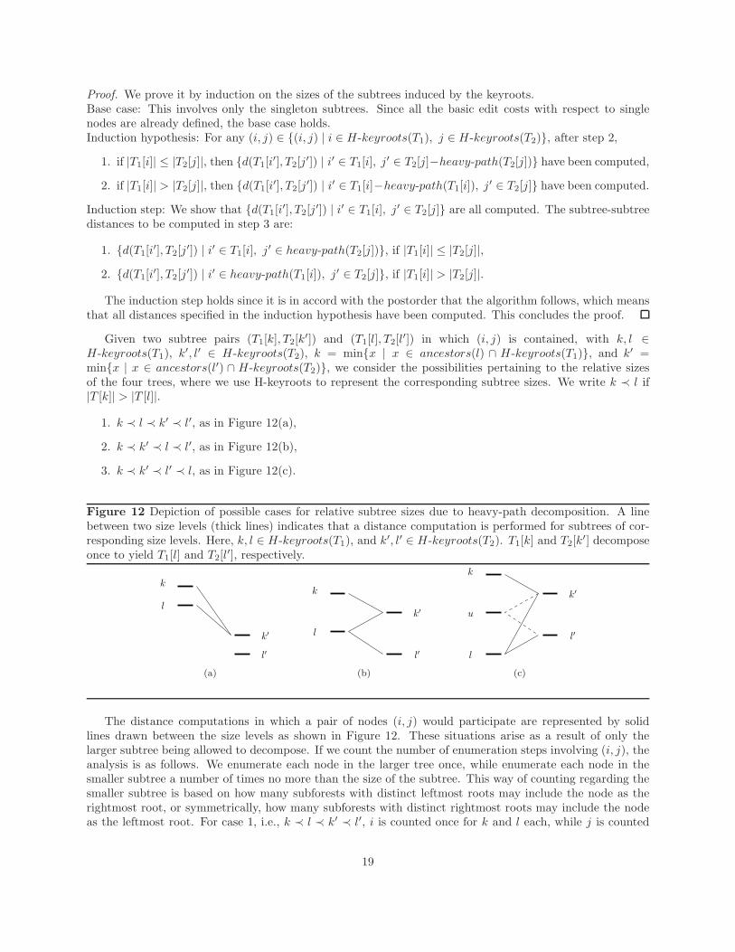
Given two subtree pairs (T1[k], T2[k′]) and (T1[l], T2[l

′]) in which (i, j) is contained, with k, l ∈H-keyroots(T1), k′, l′ ∈ H-keyroots(T2), k = minx | x ∈ ancestors(l) ∩ H-keyroots(T1), and k′ =minx | x ∈ ancestors(l′) ∩ H-keyroots(T2), we consider the possibilities pertaining to the relative sizesof the four trees, where we use H-keyroots to represent the corresponding subtree sizes. We write k ≺ l if|T [k]| > |T [l]|.

1. k ≺ l ≺ k′ ≺ l′, as in Figure 12(a),

2. k ≺ k′ ≺ l ≺ l′, as in Figure 12(b),

3. k ≺ k′ ≺ l′ ≺ l, as in Figure 12(c).

Figure 12 Depiction of possible cases for relative subtree sizes due to heavy-path decomposition. A linebetween two size levels (thick lines) indicates that a distance computation is performed for subtrees of cor-responding size levels. Here, k, l ∈ H-keyroots(T1), and k′, l′ ∈ H-keyroots(T2). T1[k] and T2[k

′] decomposeonce to yield T1[l] and T2[l

′], respectively.

k

l′

k′

l

(a)

k′

k

l

l′

(b)

k′

k

l

u

l′

(c)

The distance computations in which a pair of nodes (i, j) would participate are represented by solidlines drawn between the size levels as shown in Figure 12. These situations arise as a result of only thelarger subtree being allowed to decompose. If we count the number of enumeration steps involving (i, j), theanalysis is as follows. We enumerate each node in the larger tree once, while enumerate each node in thesmaller subtree a number of times no more than the size of the subtree. This way of counting regarding thesmaller subtree is based on how many subforests with distinct leftmost roots may include the node as therightmost root, or symmetrically, how many subforests with distinct rightmost roots may include the nodeas the leftmost root. For case 1, i.e., k ≺ l ≺ k′ ≺ l′, i is counted once for k and l each, while j is counted

19

|T2[k′]| steps for k′, for a total of 2|T2[k

′]| steps. For case 2, i.e., k ≺ k′ ≺ l ≺ l′, (i, j) is counted 1× |T2[k′]|

steps for (k, k′), |T1[l]|×1 steps for (l, k′), and 1×|T2[l′]| steps for (l, l′), for a total of |T2[k

′]|+ |T1[l]|+ |T2[l′]|

steps. For case 3, i.e., k ≺ k′ ≺ l′ ≺ l, (i, j) is counted 1× |T2[k′]| steps for (k, k′), |T1[l]| × 1 steps for (l, k′),

and |T1[l]| × 1 steps for (l, l′), for a total of |T2[k′]| + 2|T1[l]| steps. In the time complexity analysis, the

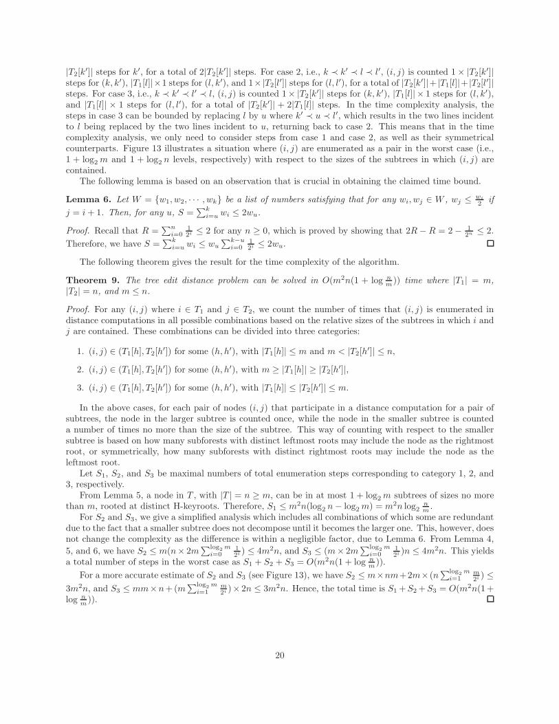
steps in case 3 can be bounded by replacing l by u where k′ ≺ u ≺ l′, which results in the two lines incidentto l being replaced by the two lines incident to u, returning back to case 2. This means that in the timecomplexity analysis, we only need to consider steps from case 1 and case 2, as well as their symmetricalcounterparts. Figure 13 illustrates a situation where (i, j) are enumerated as a pair in the worst case (i.e.,1 + log2 m and 1 + log2 n levels, respectively) with respect to the sizes of the subtrees in which (i, j) arecontained.

The following lemma is based on an observation that is crucial in obtaining the claimed time bound.

Lemma 6. Let W = w1, w2, · · · , wk be a list of numbers satisfying that for any wi, wj ∈ W , wj ≤wi

2if

j = i+ 1. Then, for any u, S =∑k

i=u wi ≤ 2wu.

Proof. Recall that R =∑n

i=012i≤ 2 for any n ≥ 0, which is proved by showing that 2R− R = 2 − 1

2n≤ 2.

Therefore, we have S =∑k

i=u wi ≤ wu

∑k−u

i=012i≤ 2wu.

The following theorem gives the result for the time complexity of the algorithm.

Theorem 9. The tree edit distance problem can be solved in O(m2n(1 + log nm)) time where |T1| = m,

|T2| = n, and m ≤ n.

Proof. For any (i, j) where i ∈ T1 and j ∈ T2, we count the number of times that (i, j) is enumerated indistance computations in all possible combinations based on the relative sizes of the subtrees in which i andj are contained. These combinations can be divided into three categories:

1. (i, j) ∈ (T1[h], T2[h′]) for some (h, h′), with |T1[h]| ≤ m and m < |T2[h

′]| ≤ n,

2. (i, j) ∈ (T1[h], T2[h′]) for some (h, h′), with m ≥ |T1[h]| ≥ |T2[h

′]|,

3. (i, j) ∈ (T1[h], T2[h′]) for some (h, h′), with |T1[h]| ≤ |T2[h

′]| ≤ m.

In the above cases, for each pair of nodes (i, j) that participate in a distance computation for a pair ofsubtrees, the node in the larger subtree is counted once, while the node in the smaller subtree is counteda number of times no more than the size of the subtree. This way of counting with respect to the smallersubtree is based on how many subforests with distinct leftmost roots may include the node as the rightmostroot, or symmetrically, how many subforests with distinct rightmost roots may include the node as theleftmost root.

Let S1, S2, and S3 be maximal numbers of total enumeration steps corresponding to category 1, 2, and3, respectively.

From Lemma 5, a node in T , with |T | = n ≥ m, can be in at most 1 + log2 m subtrees of sizes no morethan m, rooted at distinct H-keyroots. Therefore, S1 ≤ m2n(log2 n− log2 m) = m2n log2

nm.

For S2 and S3, we give a simplified analysis which includes all combinations of which some are redundantdue to the fact that a smaller subtree does not decompose until it becomes the larger one. This, however, doesnot change the complexity as the difference is within a negligible factor, due to Lemma 6. From Lemma 4,

5, and 6, we have S2 ≤ m(n× 2m∑log

2m

i=012i) ≤ 4m2n, and S3 ≤ (m× 2m

∑log2m

i=012i)n ≤ 4m2n. This yields

a total number of steps in the worst case as S1 + S2 + S3 = O(m2n(1 + log nm)).

For a more accurate estimate of S2 and S3 (see Figure 13), we have S2 ≤ m×nm+2m× (n∑log

2m

i=1m2i) ≤

3m2n, and S3 ≤ mm×n+(m∑log

2m

i=1m2i)× 2n ≤ 3m2n. Hence, the total time is S1+S2+S3 = O(m2n(1+

log nm)).

20

Figure 13 Depiction of the situation where (i, j) are enumerated as a pair in the worst case (i.e., 1+ log2 mand 1 + log2 n levels, respectively) with respect to the sizes of subtrees in which (i, j) may be contained.Levels of different sizes are represented by thick lines. A line is drawn between two size levels to indicateinclusion of (i, j) where an arrowhead points to the smaller size. For size levels no more than m, two typesof arrowheads (filled and hollow) are used to distinguish between alternative sequences of decompositionswhere the same sequence can be traced by following the lines with same type of arrowheads.

2m

m

m

22

m

23

2

1

m

2

m

m

22

m

23

2

1

m

2

n

n

2

22m

21

Remark: It has been shown that there exist trees for which Ω(m2n(1+log nm)) time is required to compute

the distance no matter what strategy is used [4].

Theorem 10. The new algorithm solves the tree edit distance problem in O(mn) space where |T1| = m,|T2| = n, and m ≤ n.

Proof. The method is same as that described in Theorem 7.

The efficiency of the algorithm can be tightened up by combining all three path decomposition strategies(i.e., leftmost, rightmost, and heavy paths) to yield an algorithm with the least total enumeration steps.The basic idea, while retaining the general framework of the algorithm, is to recursively count the numberof enumeration steps resulted from different types of path decompositions without actually carrying outthe distance computations within the original algorithm. This means that for any d(T1[i], T2[j]) to becomputed by the algorithm, step 3 counts the number of enumeration steps involving the nodes on the pathfor (T1[i], T2[j]) with respect to each type of decomposition, while the steps involving other nodes that donot belong to the path are counted recursively at step 2 (i.e., one recursive call for each type of path) andcombined with the counts in step 3 so as to decide which path to use for that level. The results from eachlevel are recorded into a table which consumes O(mn) space. The recorded information is then used to guidethe distance computations in the selection of strategy at each step. This yields an overall least total numberof enumeration steps with respect to all strategies considered. The time complexity, however, remains thesame due to the above remark regarding the lower bound.

4 Conclusions

This article considers the tree edit distance problem and formulation of solutions in the form of recursion. Inparticular, a class of algorithms based on closely related decomposition schemes for computing the tree editdistance between two ordered trees are reviewed, with an attention to aspects of time complexity analysis.

As a summary of the contents presented in Section 3, we recapture the related path-decompositionstrategies as follows.

Leftmost paths: d(T1, T2) is computed as follows.

1. Recursively, compute d(T1[k], T2) and d(T1, T2[k′]), with k being the set of nodes connecting directly

to leftmost-path(T1) with single edges, whereas k′ being the set of nodes connecting directly toleftmost-path(T2) with single edges.

2. Compute d(T1, T2) by enumerating relevant subforests of T1 and T2 in LR-postorder.

Heavy paths on one tree: d(T1, T2) is computed as follows.

1. Recursively, compute d(T1, T2[k]) with k being the set of nodes connecting directly to heavy-path(T2)with single edges.

2. Compute d(T1, T2) by enumerating relevant subforests of T1 in prefix-suffix or suffix-prefix postorder,and relevant subforests of T2 in H-postorder.

Heavy paths on both trees: d(T1, T2) is computed as follows, assuming that |T1| ≤ |T2|.

1. If |T1| > |T2|, compute d(T2, T1).

2. Recursively, compute d(T1, T2[k]) with k being the set of nodes connecting directly to heavy-path(T2)with single edges.

3. Compute d(T1, T2) by enumerating relevant subforests of T1 in prefix-suffix or suffix-prefix postorder,and relevant subforests of T2 in H-postorder.

22

All of the above strategies can be equivalently stated as applying Equation 2 according to predefineddirections without recursing into subproblems already computed.

References

[1] P. Bille. A survey on tree edit distance and related problems. Theoretical Computer Science, 337:217–239, 2005.

[2] S. Chen and K. Zhang. An improved algorithm for tree edit distance with applications to rna comparison.Journal of Combinatorial Optimization, 27(4):778–797, 2014.

[3] W. Chen. New algorithm for ordered tree-to-tree correction problem. Journal of Algorithms, 40(2):135–158, 2001.

[4] E. D. Demaine, S. Mozes, B. Rossman, and O. Weimann. An optimal decomposition algorithm for treeedit distance. ACM Transactions on Algorithms (TALG), 6(1):2:1–2:19, 2009.

[5] S. Dulucq and H. Touzet. Decomposition algorithms for the tree edit distance problem. Journal ofDiscrete Algorithms, 3:448–471, 2005.

[6] D. Harel and R. E. Tarjan. Fast algorithms for finding nearest common ancestors. SIAM Journal ofComputing, 13(2):338–355, 1984.

[7] P. N. Klein. Computing the edit-distance between unrooted ordered trees. In Proceedings of the 6thEuropean Symposium on Algorithms(ESA), pages 91–102, 1998.

[8] M. Pawlik and N. Augsten. Rted: A robust algorithm for the tree edit distance. In Proceedings of the38th International Conference on Very Large Data Bases, volume 5, pages 334–345, 2012.

[9] M. Pawlik and N. Augsten. A memory-efficient tree edit distance algorithm. In Proceedings of the 25thInternational Conference on Database and Expert Systems Applications (LNCS), volume 8644, pages196–210, 2014.

[10] D. D. Sleator and R. E. Tarjan. A data structure for dynamic trees. Journal of Computer and SystemSciences, 26:362–391, 1983.

[11] K. Tai. The tree-to-tree correction problem. Journal of the Association for Computing Machinery(JACM), 26(3):422–433, 1979.

[12] R. A. Wagner and M. J. Fischer. The string-to-string correction problem. Journal of the ACM,21(1):168–173, 1974.

[13] K. Zhang and D. Shasha. Simple fast algorithms for the editing distance between trees and relatedproblems. SIAM Journal on Computing, 18(6):1245–1262, 1989.

23