A reliability study of electronic components and electret foils ...

ISRN KTH/EKT/FR-2003/2-SE

A reliability study of electronic components andelectret foils, including latent failures due to

submission to electrostatic dischargesin a historical retrospective.

Sten Hellstrom

KTH, Royal Institute of Technology

Department of Microelectronics and Information Technology

Solid State Devices

Stockholm 2003

A reliability study of electronic components andelectret foils, including latent failures due tosubmission to electrostatic dischargesin a historical retrospective.

A dissertation submitted to Kungliga Tekniska Hogskolan,Stockholm, Sweden, in partial fulfillment of therequirements for the degree of Teknologie Doktor.

c© 2003 Sten HellstromKTH, Royal Institute of TechnologyDepartment of Microelectronics and Information TechnologyElectrum 229SE-16440 KistaSweden

ISRN KTH/EKT/FR-2003/2-SEISSN 1650-8599TRITA-EKTForskningsrapport 2003:2

Typeset in pdfLATEX by Sciencetronics using the memoir class

Printed in 100 copies by Universitetsservice US AB, Stockholm 2003

Dedication

to my wife and late parents and grand parentsplus all stimulating cats of our household

Motto

”Blott enkelheten som arvedel”Only by starting with a simple assumption you canhandle complex problems and attain reliable results!

Hellstrom, Sten: A reliability study of electronic components and electret foils,including latent failures due to submission to electrostatic discharges in a his-torical retrospective, ISRN KTH/EKT/FR-2003/x-SE, KTH Royal Institute ofTechnology, Department of Microelectronics and Information Technology, Stock-holm 2003.

AbstractThis thesis deals with the reliability and life-time of electronic components andways to determine these factors. Plastic encapsulated and open test circuits wereassessed at different humidity and temperature conditions. From the results anacceleration factor could be derived using the Arrhenius relation. This factoris used to determine failure rates at different drift conditions under acceleratedtest conditions. A formula for the factor containing both relative humidity andtemperature could be established and was found to hold also for measurementspublished by others.

Electrostatic discharge (ESD) transients were studied experimentally and bysimulation with good agreement. A very sensitive method to detect latent failuresof two kinds was introduced by nonlinearity measurements utilizing the thirdharmonic of a test signal. The ESD-susceptibility dependence on design andtechnology is shown and can be used to improve built-in reliability.

Influences in the performance of semiconductor devices from defects like fixedcharges and ions were interpreted for the first time by simulation using a 2D-finite element component program. Significant results gave an application toa MOSFET device showing parameter derating, especially the change of thethreshold value. A short description of later development in simulation methodswith new, more powerful tools improving component performance and reliabilityis given.

Charged thin films of Teflon, so called electrets, are used as microphone mem-branes. The electret voltage is a suitable reliability factor. From experimentalresults a mathematical relation including the temperature was established forthe rate of decay of the electret voltage with time. A method to charge theelectrets with radioactive sources is outlined and described in a patent.

Finally an attempt was done to analyze the reliability of thin film circuits bymathematical methods. Bell Labs introduced RC-feedback filters realized intantalum thin film technology. The phase shift of the filter is about π or 180. Amathematical apparatus was developed to calculate the change in frequency andattenuation from small component variations in resistors and capacitors. Firstand higher order corrections were derived, using expansion by the Taylor seriesfor the higher order.

Keywords: reliability, failure mechanism, acceleration tests, ESD, latent fail-ure, plastic encapsulation, electret, thin film

Contents

Acknowledgements vii

Summary ix

Moisture and evaluation of accelerated testing . . . . . . . . . ix

ESD investigations . . . . . . . . . . . . . . . . . . . . . . . . x

Simulation of MOSFET-devices . . . . . . . . . . . . . . . . . xi

Teflon electrets . . . . . . . . . . . . . . . . . . . . . . . . . . xii

Tantalum thin films . . . . . . . . . . . . . . . . . . . . . . . xiii

List of papers by the author xv

Moisture and accelerated tests . . . . . . . . . . . . . . . . . xv

Electrostatic Discharges . . . . . . . . . . . . . . . . . . . . . xvi

Device Simulation . . . . . . . . . . . . . . . . . . . . . . . . xvii

Teflon Electrets . . . . . . . . . . . . . . . . . . . . . . . . . . xviii

Tantalum Thin Films . . . . . . . . . . . . . . . . . . . . . . xviii

Publications by the author in other fields . . . . . . . . . . . xix

Acronyms xxiii

1 Moisture and Accelerated Testing 1

ii CONTENTS

1.1 Introduction . . . . . . . . . . . . . . . . . . . . . . . . . 1

1.2 Moisture in Encapsulation . . . . . . . . . . . . . . . . . 2

1.2.1 Accelerated Testing . . . . . . . . . . . . . . . . 4

1.2.2 Theoretical Models . . . . . . . . . . . . . . . . . 4

1.2.3 Further Investigations . . . . . . . . . . . . . . . 12

1.3 Experimental Conditions and Results . . . . . . . . . . . 21

1.3.1 Other Approaches . . . . . . . . . . . . . . . . . 30

1.3.2 An Example of Evaluation of Accelerated Tests . 40

1.4 References . . . . . . . . . . . . . . . . . . . . . . . . . . 46

2 ESD Investigations 55

2.1 Introduction . . . . . . . . . . . . . . . . . . . . . . . . . 55

2.2 ESD-Testing and Models . . . . . . . . . . . . . . . . . . 56

2.2.1 General . . . . . . . . . . . . . . . . . . . . . . . 56

2.2.2 Human Body Model . . . . . . . . . . . . . . . . 59

2.2.3 Machine Model . . . . . . . . . . . . . . . . . . . 62

2.2.4 Charged Device Model . . . . . . . . . . . . . . . 63

2.2.5 Charged Package Model . . . . . . . . . . . . . . 65

2.2.6 Charged Board Model . . . . . . . . . . . . . . . 66

2.2.7 Field Induced Model . . . . . . . . . . . . . . . . 68

2.2.8 Charged Chip Model . . . . . . . . . . . . . . . . 69

2.2.9 Triboelectricity . . . . . . . . . . . . . . . . . . . 69

2.2.10 Antistatic Materials . . . . . . . . . . . . . . . . 70

2.3 ESD-Susceptibility and Failure Mechanisms . . . . . . . 72

iii

2.3.1 Latent Failures . . . . . . . . . . . . . . . . . . . 72

2.3.2 Technology Dependence . . . . . . . . . . . . . . 73

2.4 Detection of Latent Failures . . . . . . . . . . . . . . . . 82

2.4.1 Current-Voltage Dependence . . . . . . . . . . . 82

2.5 ESD-Influence on Electronic Elements and Systems . . . 88

2.5.1 Experimental Results . . . . . . . . . . . . . . . 88

2.5.2 Latency . . . . . . . . . . . . . . . . . . . . . . . 91

2.5.3 Computer Simulation of ESD Transients . . . . . 94

2.5.4 Conclusion . . . . . . . . . . . . . . . . . . . . . 113

2.6 References . . . . . . . . . . . . . . . . . . . . . . . . . . 114

3 Simulation of MOSFET Devices 119

3.1 Introduction . . . . . . . . . . . . . . . . . . . . . . . . . 119

3.2 Simulation of Gate Oxide Failures . . . . . . . . . . . . 120

3.2.1 Theory . . . . . . . . . . . . . . . . . . . . . . . 121

3.2.2 Computer Simulations . . . . . . . . . . . . . . . 122

3.2.3 Summary of the Figures . . . . . . . . . . . . . . 125

3.3 Comments . . . . . . . . . . . . . . . . . . . . . . . . . . 133

3.4 References . . . . . . . . . . . . . . . . . . . . . . . . . . 137

4 Teflon Electrets 141

4.1 Introduction . . . . . . . . . . . . . . . . . . . . . . . . . 141

4.2 Emission of Charges from Traps . . . . . . . . . . . . . . 143

4.2.1 The Poole-Frenkel Effect . . . . . . . . . . . . . . 146

4.2.2 Internal Conduction Mechanisms . . . . . . . . . 149

iv CONTENTS

4.2.3 The Discharge Current . . . . . . . . . . . . . . . 159

4.2.4 Ionization Energy . . . . . . . . . . . . . . . . . 164

4.3 Determination of Model Parameters . . . . . . . . . . . 166

4.3.1 Check of Decay Measurement Results . . . . . . 166

4.3.2 Estimation of the Average Ionization Energy . . 174

4.4 Summary and Conclusion . . . . . . . . . . . . . . . . . 174

4.4.1 Charge Maintenance by Radioactive Irradiation . 177

4.5 References . . . . . . . . . . . . . . . . . . . . . . . . . . 181

4.6 Appendix . . . . . . . . . . . . . . . . . . . . . . . . . . 184

5 Tantalum Thin Films 189

5.1 Introduction . . . . . . . . . . . . . . . . . . . . . . . . . 189

5.2 Theoretical Approach . . . . . . . . . . . . . . . . . . . 191

5.3 Applications . . . . . . . . . . . . . . . . . . . . . . . . . 193

5.3.1 RC Twin-T Filter Characteristics . . . . . . . . . 193

5.3.2 RC Twin-T Filters using Taylor Series . . . . . . 195

5.3.3 Influence of Component Variations on the Atten-uation . . . . . . . . . . . . . . . . . . . . . . . . 197

5.3.4 Higher Order Frequency Corrections . . . . . . . 197

5.4 Some Important Experimental Results . . . . . . . . . . 201

5.5 Conclusions . . . . . . . . . . . . . . . . . . . . . . . . . 201

5.6 References . . . . . . . . . . . . . . . . . . . . . . . . . . 204

Addendum 207

Conclusions and Summary . . . . . . . . . . . . . . . . . . . . 207

Trends in VLSI-reliability . . . . . . . . . . . . . . . . . 208

v

Note added in proof . . . . . . . . . . . . . . . . . . . . . . . 209

References . . . . . . . . . . . . . . . . . . . . . . . . . . . . . 216

Acknowledgements

Prof. Emeritus Gosta Hellgren is recognized for accepting me as a doc-toral student at the former Institution ”Applied electronics” of the RoyalInstitute of Technology, Stockholm and Prof. Sture Petersson head of theLaboratory of Solid State Electronics for taking over my work. Changeof his own duties caused my transfer to the Device Technology Labora-tory, where Prof. Mikael Ostling, today also department head took theresponsibility for the fulfilment of the thesis. He cared very much forgiving me fashionable conditions. Likewise Prof. Carl-Mikael Zetterlingkindly corrected the thesis and guided the scriptum. A thank to the restof the laboratory who accepted my presence and to the secretary ZandraLundberg for all help.

A special thanks is given to all co-authors of my publications improvingtheir value. Prof. Viktor Scuka of Uppsala University and Prof. NielsJonassen of the Technical University of Denmark influenced my ESD re-search and are recognized for that. In this context must also Dr. CharvakaDuvvury, Texas Instrument, Dallas and Mr. Masamitso Honda, Tokyo,Japan be recognized for good collaboration in the ESD field, an impor-tant part of the thesis.

Mr. Bo Bjorklund, Ericsson Telecom AB, helped a great deal at the startof the moisture investigations and is recognized for that. My thanks toSILVACO inernational, Palo Alto, California, USA for use of some of theirsimulation programs and computer facilities.

I am also obliged to the US ESD Association Standardization committeeon ESD testing models with the chairman L. R. Lesley. My thank goesalso to Mr. Christer Afzelius, Swedish Defence Materials Administration,for much help with the long run latency experiment.

viii Acknowledgements

Prof. Dr. Alessandro Birolini, Professor Emeritus of Reliability Engineer-ing at the Swiss Federal Institute of Technology (ETH) Zurich, Switzer-land, is very much appreciated for his long time support of my reliabilityresearch and for accepting to be the opponent in the oral examination ofthe thesis. For PC help to give the thesis presentation the stipulated print-ing form I am very much obliged to Mr. Sang-Kwon Lee and Mr. Sang-MoKoo of the EKT-Lab. I am also obliged to Dr. Uwe Zimmermann, KTHand Sciencetronics, for his help with reformulating the printed version tomake it more legible, improving figures, adding good comments and cor-rections. I am indebted to the Swedish Electrotechnical Comission (SEK)for supplying me with the IEC-ESD standards.

Finally I want to express my gratitude to my wife, Fusae, for her patiencewith my research work and translation of Japanese scientific papers onmy subject.

Stockholm, July 2003

Sten Hellstrom

Summary

This thesis deals with the reliability and life-time of electronic compo-nents, ways to determine it and some basic research for support of it.There are two main subjects: moisture influence on plastic encapsulatedintegrated circuits (ICs) and the implication of electrostatic dischargewith aspects of safety and functionality

Moisture and evaluation of accelerated testing

A testing philosophy was deduced and as a special new contribution ofthis work a time transformation for failure intensities at different tem-peratures could be derived. Main results as to plastic encapsulation areconfirmation of some approaches of theoretical prediction of failure rateand establishment of a closed formula using surface conductivity as a pa-rameter and corrosion of metallic conductors as failure mechanism. Manyresults from literature were penetrated together with own experimentalresults. The crucial outcome is an analytical expression for failure rate G,including both temperature T and relative humidity RH as parameters.Ea is an activation energy that depends on humidity and the corrosionalprocess. A is a constant and k the Boltzmann constant:

G = A exp−Ea

kTexp(−α RH)

(1)

The aim is to facilitate evaluation of components by so-called acceleratedtests Measurements are performed at increased temperature and moisture,giving earlier failure appearance. Measuring time can be reduced as much

x Summary

as 10 to 100 times. The acceleration factor a is given as:

a =G2

G1(2)

Where G1 and G2 are calculated by the preceding formula. The activa-tion energy is evidently a function of relative humidity RH. The param-eters are determined from a series of measurements that are described inthe work. They depend on the type of component. A confirmation ofthe expression given above was obtained in a special application, wherecomparison between 1st and 2nd order approximation of the exponentialexpression for the RH-term was possible. The advantage of the assumedmodel is that it was derived from the results of physical measurementsOther assumptions are based on mathematical expressions with parame-ters, that are evaluated from a vast experimental outcome.

ESD investigations

We start with a repetition of the fundamental methods for determinationof electrostatic discharge (ESD) influence on the components as given bydifferent applications and formulated by standardization committees, es-pecially by the US electrostatic discharge (ESD)-Association. Methodsfor checking ESD-susceptibility are very important. The present workis concentrated on study of ESD-transients in components by computersimulation. But also investigation for detection of ESD-failures and oc-currence of latent failures was done.

The method of 3rd harmonic proved to be efficient for both SiO2−layersand pn-junctions. Due to the sensitivity of the method failures couldeasily be detected. This was probably the first method of that kind. Nowthere exist other possibilities.

As to latency two modes are defined, time-dependent and event-depend-ent. The former implies that a component was submitted to an ESD-pulseas indicated by some parameter change. It is, however still working withinthe given specification for it, but after some time fails or stops working.The latter means that an ESD-disturbed component works perfectly asbefore but fails after an additional ESD-pulse with height beneath thesusceptibility level of an undamaged component. The last phenomenon iswell verified and recognized. But the first one has often been questioned.For investigation of the possibility of time-dependent latency, a popula-tion of logical circuits was submitted to different constraint after zapping

Simulation of MOSFET-devices xi

with ESD-pulses for a period of about 3 years. The items were checkedat certain intervals and compared with an unstressed population. A clearindication of time-dependent latency was obtained. These kind of inves-tigations are a strong support to an effective ESD-protection program bythe users.

The crucial simulation work was application to pn-junctions, forward orbackward operated. The heat effect due to the rapid temperature riseby fast ESD-transients was studied. Failure criteria was the meltingpoint of silicon or a negative resistance. Simulations were made bothin 1D and 2D. The results were verified by comparison with experimentalwork. The mathematical treatment of the influence of the transients onsemiconductors is obtained by solving the partial differential equationsof semiconductors coupled to the heat transport equation. Existing fi-nite element or finite difference programs were used. Proper initial andboundary conditions had to be applied. The temperature dependence ofall parameters were incorporated. The simulations can be used to de-termine parameters such as e.g. the heat distribution and the voltage ina component and to optimize the physical composition of the device bystructural changes. The best arrangement for cooling the device can alsobe elaborated. Equally important is the possibility to localize so-calledhot spots and their dependence on composition and cooling. Results in-dicate that 3D simulation would give a complete answer to the effects ofESD-transients, however 2D simulations are often sufficient. The simula-tion results were verified by comparison with experimental tests.

Simulation of MOSFET-devices

Simulation methods for electronic components were used at an early stagein the development. Now computer aided design (CAD) is an almost nec-essary tool for design of semiconductor devices and many programs on thesubject were developed. Application to study specifically the reliabilityof components came much later. But already in 1978 the author startedsimulations of MOS field effect transistors (MOSFETs) with the purposeto improve their reliability. A finite element program, HALVFEM, devel-oped at the Royal Institute of Technology was used for simulation in 2D.The aim was to investigate the influence of defects in the components,especially at the Si− SiO2 interface, on their performance. Also interfer-ence from ions (like Na+) could be found. Change of device parametersgave a measure of deterioration due to defects. The threshold voltage, for

xii Summary

instance, was revealed as a sensitive parameter. By the results obtainedthe conclusion was drawn, that simulation is an important tool to designand improve intrinsic reliability of a new component. Only five or sixyears later the electronic community took up this kind of application.

Teflon electrets

In the late 1960’s a new type of membrane for microphones were intro-duced. Thin organic foil electrets came into use. An electret is a chargedorganic foil or resin. The word electret was coined by O. Heaviside in thebeginning of the 20th century, but the first usable ones were producedin Japan about 1920. At first resin substances were used, which wereinserted into a strong electric field at high temperatures. After a suitabletime span these were cooled down to room temperature and the obtainedpolarization was frozen in. Carnauba wax was the selected resin in thebeginning. When the industry introduced plastics, thin organic foils weretried for electret production in a similar way as above. Teflon foils provedto be very applicable as electrets. They give a much better character-istic, especially at high frequencies, than common magnetic membranes.An additional advantage appeared as electron bombardment of the foilscan charge them. The electrons are captured in potential traps insidethe organic foil. Discharge and depolarization of the electrets will limittheir life-length. These processes depend on temperature. Different theo-retical approaches and experimental trials were applied to determine thelife-length of electrets. The present work accounts for a new approach. Itis based on the assumption of the electret as a capacitor. The so-calledPoole-Frenkel effect is assumed to govern the emptying of the filled traps.Experimentally the electrets are kept at an elevated temperature and thecharge decay is registered by measuring the electret voltage at suitabletime intervals. Decay curves were traced and fitted to the theoreticalapproach, and a good agreement was obtained. As a replacement of theslightly ineffective method with polarization at elevated temperature, theauthor introduced an electron bombardment method of electret charg-ing. A scanning electron microscope (SEM) is used and the electret foil isattached at the target place. By defocussing the electron beam a homoge-nous bundle is obtained and the foil is charged uniformly. An additionaladvantage is that the electron energy can be adapted to fit the energyof the traps. On the author’s advice the method came into use at LMEricsson Telephone Co. for electret production. A method for electretcharging by radioisotopes was patented, see US Patent 3,949,178 (1976).

Tantalum thin films xiii

Radionuclides inside the electret will keep it charged. Life-length is aboutthe same as the half-life of the radionuclide. As one possible candidatetritium has a suitable maximum energy of about 10 kV for the beta par-ticles and half-life of about 12 years. Short lived isotopes can be usedto preserve the electret charge at transport to places with a very warmclimate. A charge amplifier for electret-microphones was analyzed by acomputer program to check its performance.

Tantalum thin films

Background for the investigations of tantalum thin films was the methodat Bell-Labs to produce RC-filters containing tantalum resistors and ca-pacitors with Ta2O5-dielectrics. The filters were used as feed-back filtersin the oscillators of so-called touch-tone telephones. The whole oscillatorwas simulated by a computer program. The thin tantalum films wereproduced by sputtering in a dc-sputtering equipment. The films weredeposited on glass substrates. By electrolyzing tantalum films, Ta2O5-dielectrics are obtained. A capacitor is prepared by covering the oxidewith layers of nichrome (NiCr) and Au. Resistors are formed from tan-talum films by an etching technique. Using so called reactive sputtering,e.g. the addition of nitrogen to the sputtering gas, the resistors will get anegative temperature coefficient. In an RC-filter such a negative tempera-ture coefficient or the resistance can compensate the positive temperaturecoefficient of the capacitors and the RC time constant will not vary withtemperature. The filters are meant to operate from −25 C to +125 C.The investigation concentrated on the possibility to find a correlation be-tween the temperature coefficient and the nitrogen doping concentrationfacilitating the production. The method of 3rd harmonic already usedin another context proved to be applicable. A statistical program wasprepared for calculation of quality and reliability of oscillators from theproduction.

xiv Summary

'

&

$

%

ProcessSimulation

e.g.TSupremeTM

'

&

$

%

DeviceSimulation

e.g. PiscesTM

MediciTM

AtlasTM

GigaTM

'

&

$

%

CircuitSimulation

e.g. SpicePSpiceTM

'

&

$

%

RelieabilitySimulation

this work

⇒ changes indevice

structure

Figure 1: This block scheme and diagram gives an overview over simulationmethods and tools, used to design, analyze and predict the reliability of semi-conductor devices, like MOSFETs and MOS-capacitors.

List of papers by the author

Moisture and accelerated tests

1. Hellstrom, S.Determination of acceleration factors for the test of plastic encap-sulated ICs by measuring the surface conductivityLM Ericsson Internal Report, 7250/X/Ag 21561980 (in Swedish).

2. Hellstrom, S.On the method of obtaining acceleration factors from surface con-ductivity measurementsLM Ericsson Internal Report, 7250/X/Ag 30161980

3. Hellstrom, S.Environment testing of plastic encapsulated cross point thyristorswith ceramic encapsulated as comparison (performed 1978 - 1979)LM Ericsson Internal Report, 7280/X/Ag 42381981 (in Swedish).

4. Hellstrom, S.Surface conductivity measurements (I)LM Ericsson Internal Report, XT/HG 15391984.

5. Hellstrom, S.Surface conductivity measurements (II)LM Ericsson Internal Report, XT/HG 16081984.

xvi List of papers by the author

6. Hellstrom, S.On the choice of component sampling, the meaning of AQL (Accept-able Quality Level) and AOQL (Average Outgoing Quality Limit)and the distribution of failure outcome at temperature acceleratedtestsLM Ericsson Internal Report, 70201/X/Ag 21291980 (in Swedish).

7. Hellstrom, S.On the choice of an average activation energy for LSI - device reli-ability evaluationLM Ericsson Internal Report, 7280/XK/Ag 43241981.

Electrostatic Discharges

8. Hellstrom, S.ESD - The Scourge of ElectronicsSpringer Verlag1998.

9. Hellstrom, S.Detection of Latent Failures in Semiconductors due to Electro-StaticDischarges4th International Conference on Reliability and Maintainability,Perros-Guirec and Tregastel, France1984.

10. Hellstrom, S.; Eklof, P. and Welander, A.Studies and Revelation of Latent ESD - FailuresProceedings of the EOS/ESD - Symposium, pp. 81–911986.

11. Hellstrom, S. and Welander, A.Study of Time - Dependent Latency in a Logical MicrocircuitProceedings ESREF’91, p. 1011991.

12. Hellstrom, S. and Eriksson, L.-O.Simulation of Transients in pn-JunctionsProceedings EUROSTAT’90, Barbican, London1990.

Device Simulation xvii

13. Hellstrom, S.; Freydin, B.; Velmre, E. and Udal, A.Numerical Simulation of Electrothermal Effects in ESDProceedings ESREF’921992.

14. Hellstrom, S.; Freydin, B.; Udal, A. and Velmre, E.Two-Dimensional Modelling of Selfheating Processes in Semicon-ductor DevicesProceedings of the 2nd Pan European ESD-Symposium and Exhi-bitionStrasbourgh, France1993.

15. Hellstrom, S.Simulation of Electrothermal Effects in Semiconductors, exposed toESD TransientsInvited paper at the XXIVth General Assembly of the Int. Unionof Radio Science (URSI)Kyoto, Japan1993.

Device Simulation

16. Hellstrom, S.Simulation of structures, I.LM Ericsson Internal Report, 1509/X/Ag 30061980.

17. Hellstrom, S. and Arnborg, T.Contribution to the SNRV-50-year anniversary SEMINARSLM Ericsson Internal Report, 7280/XK/Ag 43131981.

18. Hellstrom, S. and Arnborg, T.Gate oxide failures in MOSFET - Devices studied by a simulationmethodRELECTRONIC’82, Budapest, Hungary1982.

19. Andersson, C.A literature search on the importance of defects for oxide breakdownin MOS-structures, especially defects at the Si/SiO2-interface

xviii List of papers by the author

TRITA-FYS-3005, Royal Institute of Technology, Stockholm, Swe-denMaster thesis, performed at Ericsson TelecomSupervisor: Hellstrom, S.1986 (in Swedish).

Teflon Electrets

20. Wesemeyer, H. and Hellstrom, S.On the discharge of electretsEricsson Technics, No. 3, pp. 220–2461977.

21. Hellstrom, S.Verification of the Poole - Frenkel effect in an electret dischargeLM Ericsson Technical Report, MeT 77081977 (in Swedish).

22. Wesemeyer, H. and Hellstrom, S.Discharge of electrets by electric field enhancement of thermo-ionicemission: Improvement of a proposed theoryEricsson Technics, No. 2, pp. 108–1281978.

Tantalum Thin Films

23. Hellstrom, S.The frequency change due to small component variations in passiveRC Twin-T filters with π rad phase shiftEricsson Technics, No. 1, p. 251971.

24. Hellstrom, S.Second order frequency corrections and attenuation relations of RCTwin-T filters with π rad phase shiftEricsson Technics, No. 3, p. 1371971.

25. Hellstrom, S.LM Ericsson Telephone Co., Materials Lab. Report, No. 728240/Mgf 2811970 (in Swedish).

Publications by the author in other fields xix

26. Hellstrom, S.LM Ericsson Telephone Co., Materials Lab. Report, No. Mgf 4151972 (in Swedish).

27. Hellstrom, S. and Wesemeyer, H.Nonlinearity measurements of thin filmsVacuum, Vol. 27, No. 4, pp. 339–3431977.

28. Hellstrom, S.Current applications of R- and RC- network circuits performed inthin tantalum filmsLM Ericsson Telephone Co., Materials Lab. Report, No. Mgf 3821971 (in Swedish).

29. Hellstrom, S. and Magnusson, M.Method for Monte - Carlo - Analysis of RC - FiltersLM Ericsson Telephone Co., Materials Lab. Report, No. Mgf 4631972 (in Swedish).

30. Hellstrom, S.; Leringe, M.; Karlsson, B. and Control-Data SwedenPractical User Manual in Applying the Circuit Programs DICAPand TRACAP, especially with a Routine for Monte-Carlo-Analysisof oscillators in Touch Tone Telephones, giving specifically the oscil-lators transmission frequencies, generated by the RC-feedback filterLM Ericsson Telephone Co., Materials Lab. Report, No. Mgf 576:11973 (in Swedish).

31. Isaksson, K. and Hellstrom, S.Method for automatic frequency trimming of RC-oscillatorsLM Ericsson Internal Report, MeT 77061977 (in Swedish, abstract in English).

Publications by the author in other fields

32. Hansen, H. and Hellstrom1, S.The EC-decay of Tm 170Zeitschrift fur Physik, Bd. 223, pp. 139–1441969.

1Publications 32, 33 and 34 formed a Technology Licentiate degree for S. Hell-strom, according to the old educational system at the Royal Institute of Technology,Stockholm, Sweden , 1971.

xx List of papers by the author

33. Hellstrom1, S. and Brune, D.Determination of the absolute disintegration rate of Cs137-sourcesby the tracer methodNukleonik, Bd. 6, Heft 4, pp. 174–1781964.

34. Hellstrom1, S.; Brune, D. and Dubois, J.Improvements in applied gamma ray spectroscopyNukleonik, Bd. 7, Heft 8, pp. 484–4881965.

35. Hellstrom, S.On the use of Niobium as a neutron dose monitorSwedish Atomic Energy Co., Report AE-FFN-74, 1967 andNuclear Science Abstract, NSA 22:28 177, 1968.

36. Hellstrom, S.Proportional countersProceedings of IAEA - Symposium on the Standardization of Ra-dionuclides, Vienna1959.

37. Hellstrom, S.Absolute measurements by means of liquid scintillatorsProceedings of the Fifth Int. Instrument and Measurement Confer-ence, pp. 631–640Stockholm, Sweden, 19601960.

38. Hellstrom, S.On the Standardization of Radioactive IsotopesTVF 31, No. 6, pp. 255–2631960 (in Swedish).

39. Hellstrom, S.An accurate method to determine the Au198-activity in neutron ir-radiated gold foilsSwedish Atomic Energy Co., Report AE-FFN-21964.

40. Hellstrom, S. and Malmskog, S.On the use of (n, n′, γ) reactions as threshold detectorsSwedish Atomic Energy Co., Report AE-RFA-5801964.

Publications by the author in other fields xxi

41. Hellstrom, S. and Malmskog, S.Measurement of the life-time of the 396.3 kV level in Lu175 andinvestigation of the γ-transitions in the decay of Y175 → Lu175 byGe(Li)-detector1964 (unpublished).

42. Hellstrom, S.Investigation of highly excited nuclear levels by nuclear resonancescattering of neutron capture gamma raysSwedish Atomic Energy Co., Preliminary Report1967–1968.

Some results obtained are angular distribution curves of:a) 7.01 MeV transition in Sn excited by a Cu-sourceb) 6.41 MeV transition in La139 excited by a Ti-source,curve fitted to W (θ) = 2.6 + 0.81 cos2(θ), θ is the angle betweenincident and scattered γ-ray. c) the angular intensity anisotropyof Cd 7.72± 0.05 MeV emission, photo-excited with a Fe57 promptgamma source.d) spectrum of γ-transition in La2O3, measured at scattering angle135 : 4.32 MeV, 4.83 MeV, 5.38 MeV, 5.82 MeV, 6.41 MeV

43. Hellstrom, S.Electrical and magnetic properties of thin films and Measurementsand properties of thin filmsin Ed. Brune, D. et al.: Surface CharacterizationWiley-VCH, pp. 534–5621997.

44. Hellstrom, S.Advanced House Livingin Ed. Brune, D. et al.: The Global EnvironmentWiley-VCH, p. 12341997.

45. Hellstrom, S.Vision of the future society: Advanced House Livingin Domotic, Environment and UsersWorkshop at the 14th Conf. of the Int. Association for People-Environment StudiesStockholm, 1996.

46. Rejdin, A. and Hellstrom, S.Systems and Components: Computer based Systems with Compo-nents for the Ruling and Survey of Buildings

xxii List of papers by the author

Swedish Council of Building Construction, Report R271992 (in Swedish).

47. Hellstrom, S.Technical expert report, Nuclear instrumentationTechnical Assistance-Report No. 837Report to the Government of Ghana and IAEA, Vienna1973.

S. Hellstrom is an ESD engineer certified by National Association of Radio& Telecommunications Engineers, USA (NARTE) and member of the USESD Association. For about ten years he participated in two CenelecElectronic Components Committee (CECC) work groups on reliability.He was also a board member of the European ESD Association.

Acronyms

ANSI American National Standards InstituteAOQ Average Outgoing QualityAQL Acceptable Quality LevelBPO British Post OfficeCAD computer aided designCCM Charged Chip ModelCDM Charged Device ModelCECC Cenelec Electronic Components CommitteeCLTE component linearity test equipmentCMOS complementary MOSCNET French National Center for TelecommunicationsCPM Charged Package ModelCSF charge sharing factorCV capacitance versus voltageDIL dual in-line, IC package typeDIP dual in-line packageDFT density-functional theoryDRAM dynamic RAMDUT device under testEBIC electron beam induced currentECL emitter-coupled logicEMMI emission microscopyEOS electrostatic overstressEPA electrostatic protected areasESD electrostatic dischargeFASTTM Fairchild Advanced Schottky TTL

xxiv Acronyms

FEP fluorinated ethylene propylene polymer, TeflonTM

FET field effect transistorFIM Field Induced ModelFNP fluorinated polymerHAST high acceleration saturated temperature testsHBM Human Body ModelHBT hetero-junction bipolar transistorHCMOS high-speed CMOSHEMT high electron-mobility transistorHTOL high temperature storage/operating life testsHTSL high temperature storage life testsIC integrated circuitIR infraredIT information technologyIV current versus voltageLSI large scale integrationLSTTL low-power Schottky TTLMIL-HDBK US Military HandbookMM Machine ModelMOS metal-oxide-semiconductorMOSFET MOS field effect transistorMTTF meantime to failureNARTE National Association of Radio & Telecommunications Engi-

neers, USANiCr nichromeNMOS n-channel MOSNRL US Naval Research LabNTT Nippon Telegraph and Telephone CorporationOCN O-Cresole Novolac-resinOEM Original Equipment ManufacturerPCB printed circuit boardPDE partial differential equationsPEM plastic encapsulated modulePFA perfluoro-alkoxy polymer, TeflonTM

ppm parts per millionPTFE poly tetra flour ethylene, TeflonTM

PVC poly vinyl chlorideRAM random access memory

Acronyms xxv

RC resistor-capacitorRH relative humidityRPP Reliability Prediction Procedure (Bellcore)RTV room-temperature vulcanizingSAM scanning acoustic microscopySEK Swedish Electrotechnical ComissionSEM scanning electron microscopeSOI silicon-on-insulatorSOT small-outline transistorSPC statistic process controlTHB temperature-humidity-biasedTHD total harmonic distortionTSC thermally stimulated currentTTC triple-track conductorTTL transistor-transistor logicULSI ultra large scale integrationVLSI very large scale integration

1Moisture and Accelerated Testing

1.1 Introduction

From late 1950’s to middle 1980’s there was a heavy development of thenew semiconductor technology. Especially the new technique with ICs,large scale integrations (LSIs) and ultra large scale integrations (ULSIs)gave rise to sophisticated methods for evaluation of their performance,quality and reliability. This formed a proper basis for today’s applica-tions and further research with a revolution of services in the modernsociety, often summarized in information technology (IT). This work isboth an overview of some relevant issues and contributions, that becameimportant. Most is concentrated on plastic encapsulation as this tech-nique implied both a simpler fabrication and cost reduction. For theperformance of the devices, ESD and its influence in electronics is an im-portant aspect. Besides the two main topics mentioned, issues in someapplication fields with great technological improvements will be described.

With the advent of microcircuits for application in the telecommunica-tion industry during the 1960’s and 1970’s reliability and life-time forcomponents became a major concern. Failure modes are recorded and byusing advanced instrumentation, failure mechanisms can be revealed. To

2 Moisture and Accelerated Testing

discard weak parts from a population a so called burn-in process is used,i.e. the components are operated at an elevated temperature for a shortertime (a few hours to some days). This is a method to determine thelife-time of components. If the influence of stress factors as temperature,moisture, electric field strength is known an acceleration factor can becalculated, which gives the relation between fall-out at accelerated andnormal conditions. Thus life-time is obtained from results of short-timeaccelerated tests. Because of the rapid development in the integrationrate of modern microcircuits failure determination is sometimes a ratherdelicate problem.

1.2 Moisture in Encapsulation

With the introduction of plastic encapsulation admitting the penetrationof moisture, corrosional effects also had to be considered. In general thebehavior of a semiconductor as a function of the temperature is describedby the Arrhenius expression:

y = Ae−Ea/kT (1.1)

where y is some component parameter, k is the Boltzman constant, T theabsolute temperature in K and Ea is the corresponding activation energyfor some failure mechanism that can change y. For plastic encapsulateddevices the problem arose how to include corrosion by moisture as a failuremechanism in the above explained sense. As corrosion in this case isan electrolytic process, surface conductivity became the key factor. If apotential drop exists between two conductor stripes a current will flow andinitiate a corrosional process, that depends on the relative humidity RH.Surface conductivity is a measure of the speed of the process. Already inthe early 1970’s the moisture problem in plastic encapsulated devices wasapproached in different ways. These will be referred to according to thenames of the investigators and of publications. In the very beginning theinfluence from temperature was neglected, and the surface conductivitygiven as a function of the RH-value:

σ = f(RH) (1.2)

1.2. Moisture in Encapsulation 3

(a) Triple track pattern (b) Meander pattern

Figure 1.1: Test structures for surface conductivity measurements. (afterRef. [28, 65])

Reich in the USA was perhaps the first one to reformulate the Arrheniuslaw to include both temperature and moisture [62]. He made a smartattempt by adding the RH-value to the T -value in Eq. 1.1:

y = A exp(− Ea

k(T + RH)

). (1.3)

This gave a fair agreement with experimental results. Reich made an ex-periment under jungle conditions, where he hang out microcircuits thatwere attacked by the rather severe climate, but the results did not cor-relate very well with laboratory experiments. This was perhaps one ofthe reasons that many new attempts were made to find a more satisfac-tory theoretical representation for the joint temperature and humidityinfluence on plastic encapsulated devices. The British Post Office (BPO)started similar experiments at about the same time in Ipswich, UK.


1.2.1 Accelerated Testing

The interpretation of the BPO tests resulted in the following formula [41]:

a = exp[4.4× 10−4

(RH2

s − RH2o

)+ 6.96× 103

(1To− 1Ts

)]. (1.4)

Here a is the acceleration factor between two test conditions o and s, i.e.how much longer time it takes at condition o to get the same results as ats. This formula was found to agree well with the factors obtained fromsome epoxy encapsulated devices in all but the severest test conditions.The factor 4.4 is a mean normalization value. Sometimes a value as highas 8 can be found. The influence of moisture is represented by the factorRH2, because the water content of the plastic should be proportional tothat factor. In these two approaches referred to, the activation energyEa is anticipated to be independent of temperature T and humidity RH.Results by Sbar and Kozakiewiecz [65] and Hellstrom [28] show that Ea

can depend on both temperature and humidity.

1.2.2 Theoretical Models

Eq. 1.4 represents the first more complete model for accelerated tests.The experiments of Sbar et al. will be outlined [65]. This because theymade rather well designed and multiple measurements with reliable re-sults. They anticipated a linear relationship between the activation energyEa and relative humidity RH. The applicability of this was proved byHellstrom through a true derivation of an exponential function [28, 30].In one case they used a triple-track conductor (TTC) pattern for theirsurface conductivity measurements (see Fig. 1.1) on ceramics and othercommercial surfaces of three characteristics: Si3N4-passivation on initialSiO2 with Ti-Pd-Au metallization pattern, alumina with the same pattern(referring to the dual dielectric used in some metal-oxide-semiconductor(MOS)-devices), Si3N4-passivation with Ti-TiN-Pt-Au pattern (fabricatedby the uniform gold process described by Labuda [40]).

One tester series had plastic encapsulation, the others were unencapsu-lated. Isothermal experiments were realized with testers in Table 1.1 tostudy the effects of humidity, temperature and bias on surface conduc-tivity. To obtain stabilized testing conditions before measurements the


Table 1.1: Test Specimens—Isothermal Experiment. (after Ref. [65])

No. Type Surface Metallization Bias[ V]

16 Triple Track Ceramics Ti-Pd-Au 4016 Triple Track Ceramics Ti-Pd-Au 10016 Triple Track Ceramics Ti-Pd-Au 18016 Test Chip (1) Si3N4 Ti-Pd-Au 1016 Test Chip (2) Al2O3 Ti-Pd-Au 1016 Test Chip (3) Si3N4 Ti-TiN-Pt-Au 10

substrate had to equilibrate without bias 24 hours at intended temper-ature and humidity whereupon they were biased for 2 hours. Appliedbiases were 40, 100, and 180 V. As a complement samples according toTable 1.2 were used at constant 80%RH and 10 or 100 V bias. Typicaltest results from different samples pattern are given in Fig. 1.2.

These results were interpreted by the author in a different way than by theinvestigators to find a physical basis for their approach. The conductivitywas traced as a function of absolute temperature with RHas a parameter.A bundle of linear curves cover the results rather well except for 65 Cas seen from Fig. 1.3. The results at this temperature in Fig. 1.2(a) also

(a) Triple track conductors, 100Vbias.

(b) Al2O3 metallization testers,10 V bias.

Figure 1.2: Surface conductivity versus RHfor different test structures. (af-ter Ref. [65])


Table 1.2: Test Specimens—Constant Humidity Experiment. (after Ref. [65])

No. Type Surface Encapsulant Bias[ V]

10 Triple Track Ceramics none 10010 Triple Track Ceramics DC 3-6550 10010 Test Chip Si3N4 none 105 Test Chip Si3N4 DC 3-6550 10

show a different trend than the others, probably due to measuring faults.Figs. 1.2(b) and 1.3(b) give results with Al2O3 metallization testers. Fol-lowing theoretical approach could be done:

logG = logG0 +Ea

k

(1T− 1T0

). (1.5)

Where G0 is constant, Ea a function of RH. Ea can be determined fromthe slopes of the curves. We see from Fig. 1.4 that a linear relationship ismost likely between Ea and RH, which is anticipated by the investigators.For an overall validity compare results by Hellstrom [31, 32]. Comparisonin Fig. 1.2(a) with the encapsulated tester reveals a substantially reducedconductivity, i.e. improved reliability. The change of Ea from negativeto positive values (Fig. 1.4) indicates a different conduction mechanismat high moisture levels. The formation of a uniform water layer on thesubstrate depends on the surface tension. At lower values of relativehumidity, even small dry islands can appear. This is also related to thesurface condition of the substrate and its composition.

Next we consider results from surface layers as presented in Fig. 1.5.Corresponding characteristics are drawn in Fig. 1.6 and the functionEa = f(RH) in Fig. 1.7. The main difference from the triple track onanother substrate (ceramics) is the constantly positive activation energyEa. A similar expression as before can be established for the conductionmechanism.

Results of measurements performed at a constant RH-value (80%) aregiven in Figs. 1.8(a) and 1.8(b). Though they are somewhat contradictoryto the earlier ones, the investigators preferred to derive the activationenergies from these only from temperature cycles with positive Ea-values,see Table 1.3. By the cycling thermal equilibrium, necessary for reliableresults, is assured.




Figure 1.3: The results of Fig. 1.2 as a function of temperature T with RHasparameter. (after Ref. [32]∗ [original figures by the author are marked with anasterisk ∗])



Figure 1.4: The activation energy Ea extracted from the data in Fig. 1.3.(after Ref. [32]∗)


Figure 1.5: Si3N4 metallization testers, 10 V bias: Surface conductivity versusRH. (after Ref. [65])

Figure 1.6: The results of Fig. 1.5as a function of temperature T withRHas parameter.

Figure 1.7: The activation energyEa extracted from the data in Fig. 1.6.(after Ref. [30]∗)



(b) Si3N4 metallization testers,10 V bias.

Figure 1.8: Surface conductivity in constant humidity experiments at80%RH. (after Ref. [65])

Table 1.3: Average activation energies at 80%RH. (after Ref. [65])

Activation energy Std. deviation[ eV]

Unencapsulated TTC .51 .14Encapsulated TTC .70 .03Unencapsulated Si3N4 test chip .46 .21Encapsulated Si3N4 test chip .64 .05

The investigators use the results of Table 1.3 together with the isotherm

logG(50 C, RH) = −18.60 + 0.062RH, (1.6)

obtained from Fig. 1.2 to generate a family of curves for G(T, RH). InFig. 1.9 the adjusted isotherms are drawn. Constant RH-values char-acteristics are replotted in Fig. 1.10. From these and assuming a lin-ear relation between activation energy Ea and relative humidity RHtheisotherms of Fig. 1.9 were calculated and from these the function Ea =f(RH) can be derived as in Fig. 1.11. The joint characteristic is given inFig. 1.12. The acceleration factor is defined as :

a =G(85 C, 85%RH)G(61 C, 85%RH)

(1.7)


Figure 1.9: Calculated isotherms(G1 vs RH) for unencapsulated tripletrack conductors. (after Ref. [33]∗)

Figure 1.10: Surface conductivity asa function of temperature with differ-ent RHvalues. (after Ref. [33]∗)

and found to be a = 105 from Fig. 1.12, while the original traces inFig. 1.9 give a = 0.7 × 105, a fair agreement supporting a unified modelto be derived later [30]. Similar results could be obtained from severalother measurements presented by the investigators. A rather extensivereliability evaluation of epoxy and plastic encapsulated devices, includ-ing also mechanical properties was performed at ERA Technology LTD,Leatherhead, UK. Some hermetic devices were tested in a similar way forcomparison. Even exposure to a tropical jungle was applied [64]. The aimwas to determine acceleration factors. Here the acceleration formula ofBPO, Eq. 1.4, was used with fairly good agreement, implicitly some con-sistence between the different acceleration formulas mentioned is given.


Figure 1.11: Activation energyas a function of RH, derived fromFig. 1.10. The different sign of theslope as compared to Fig. 1.32 de-pends on electrolytic processes. (afterRef. [33]∗)

*************************

Figure 1.12: Surface conductivityas a function of 103 exp(−0.014RH)on triple track conductors. (afterRef. [33]∗)


1.2.3 Further Investigations with Moisture in PlasticEncapsulation

Independently of previous experiments a closed formula for the influenceof moisture in plastic encapsulation was derived [28]. The following ex-pression was derived :

G = A exp[−Ea

kTexp (−α RH)

](1.8)

The factor α is found from Fig. 1.11. The relative validity of this the-oretical approach was proved already in the interpretation of the resultsof the previous investigators, see Fig. 1.12. In the findings of the closedformula for the surface conductivity several factors were considered. Thenature of the surfaces upon which the metal conductors are depositedis of importance. If SiO2 or Si3N4 are used, the phosphorous content isalso of importance. As metal, Al with different percentage of Cu or Sior both to inhibit electromigration is applied, but also nichrome (NiCr)or other combinations can appear. The presence of ions (e.g. Na+, K+,I−, Cl−, B−, S2−) will accelerate the corrosional electrolytic process. Byway of comparison also open circuit patterns were measured. Ions can beintroduced from the plastic by water penetration. Bromine is commonlyused as an additive because of its flame retardant effect on the plastic.

The author started his investigations, 1977, by using data from earliermeasurements [38, 39]. Koelsman performed measurements with a spe-cial pattern (10µm and 100µm distance between the conductor stripes,respectively) on thermal SiO2 without any protection (passivation or en-capsulation [38]). Dependent on the environment the electrolytic processis accelerating or inhibiting the corrosional effects. The latter is caused byanodization of the electrodes (e.g. Al). One series of results are demon-strated in Fig. 1.13 (Note: Au electrodes) The surface conductivity istraced as a function of the RH-values for different temperatures.

By using the values of Fig. 1.13 (interlaced line) Arrhenius plots of thefollowing form can be established, Fig. 1.14:

G = Ae−Ea( RH)/kT . (1.9)

Koelsman also gives a table for the speed of corrosion, Table 1.4.

By the technique described the joint, closed formula for the surface con-ductivity will be derived. From Fig. 1.14 the activation energies, Ea can


Figure 1.13: The surface conduc-tivity of thermal SiO2 as a function ofrelative humidity for a number of tem-perature between room temperature and100 C.

Figure 1.14: Arrhenius plots derivedfrom Fig. 1.13. (after Ref. [32, 38])

be determined and plotted as a function of relative humidity. See alsoFig. 1.15 “unencapsulated”. The curve fits to:

Ea = 0.74 e−0.0073 RH . (1.10)

For comparison with other approaches of Reich and BPO as given above,values of Fig. 1.13 are traced versus 1/(T + RH) in Fig. 1.16 and RH2

in Fig. 1.17(a), complemented with Fig. 1.17(b), which shows that theinfluence of temperature on surface conductivity is, as expected, vanish-ing for high RH-values. The same values are also plotted vs 1/RH,which were likewise used. Two areas are discernable here, 5% to 40%RHand 40% to 100%RH, see Fig. 1.18. Using the closed form given aboveand in [28] replacing Ea(RH) by the function found in Fig. 1.15 andtaking the first approximation of the exponential we trace the values vs103/[T (1 + 0.0073RH)], Fig. 1.19. Disregarding the points marked withasterisks, the values fit rather well to a straight line, from which the slope0.76 eV is derived. Compare this to 0.74 eV used in Fig. 1.15. The devi-ating points of Fig. 1.19 correspond to very low RH-values. Those of thehighest RH-values are also displaced in Fig. 1.19, but can be corrected ifhigher terms of the exponential power series are included. The analysisfairly well supports the closed form representation of surface conductivity.The same procedure was used for two cases of thermal SiO2, covered withtwo different room-temperature vulcanizing (RTV) silicone-rubber mate-


Table 1.4: Speed of Corrosion. (after Ref. [38])

Surface conductivity Time for completecorrosion of anode

[Ω−1] [s]

10−10 3× 103

10−11 3× 104

10−12 3× 105

10−13 3× 106

10−14 3× 107

10−15 3× 108

10−16 3× 109

rials, DC 90702 and DC 96084. Data is given in Figs. 1.20 to 1.23 [12]. InFig. 1.24 the result is given for DC 90702. The values are scattering morein this case than in Fig. 1.41, but the value of 1.2 eV found from the fittedline is comparable in size with 1.34 eV given in Fig. 1.15, again supportingthe closed form suggested. DC 96084 was not analyzed as Fig. 1.22 revealsa discontinuity of the activation energy also appearing in Fig. 1.15. Dis-continuities at low RH-values are probably due to a different conductionmechanism (monolayers or “islands” of water). Later an investigation ofhybrid circuits in fluorinated polymer (FNP)-plastic and silicone encap-sulation was presented [13]. Fig. 1.25 gives results of surface conductivitymeasurements with FNP-plastic and Fig. 1.26 water penetration rate forFNP (NRL) and RTV silicone. It was stated that the diffusion of waterand impurities (in the form of ions) through the FNP-plastic is extremelyslow but enough to form an electrolyte. From the curves of Fig. 1.25 theconductivity-temperature relations were derived with relative humidityRHas a parameter, Fig. 1.27(a). These were found, in the usual way, tosuit well to the following joint humidity-temperature formula :

ln(log 1017G) = A

(103

T− 2.3

)+ 2.2, A = Φ(RH) (1.11)

The slope is given by A = −(3.0 − 0.14RH), see Fig. 1.27(b). Theselast results demonstrate how much the surface conductivity depends onthe encapsulant materials used. Additional results of the same investiga-tors were interpreted and supported the closed joint representation, seeFigs. 1.28 to 1.29(b).


Figure 1.15: Activation energy as afunction of RH. (after Ref. [33]∗)

Figure 1.16: Surface conductivityas a function of 103/(T + RH). (af-ter Ref. [33]∗)

(a) linear scale (b) log-log scale

Figure 1.17: Surface conductivity as function of RH2. (The linear regressioncurves plotted in 1.17(a) are also drawn in 1.17(b).) (after Ref. [32, 38])


Figure 1.18: Surface conductivity asfunction of 1/RH. (after Ref. [32, 38])

Figure 1.19: Surface conductivityas a function of 103/(T + RH). (af-ter Ref. [32, 38])

Figure 1.20: Surface conductivityof SiO2 with DC 90702 Coating, 5µmelectrode gap. (after Ref. [12])

Figure 1.21: Surface conductivityof SiO2 with DC 96084 Coating, 5µmelectrode gap. (after Ref. [12])


Figure 1.22: Activation energy analysis for DC 96084, 5µm electrode gap.(after Ref. [12])

Figure 1.23: Activation energy analysis for DC 90702. (after Ref. [12])


Figure 1.24: Activation energy analysis for DC 90702. (after Ref. [33]∗)

Figure 1.25: Surface conductivitymeasurements with FNP plastic coatedcircuits. (after Ref. [13])

Figure 1.26: Water penetration ratefor FNP plastic (NRL) and RTV sili-cone. (after Ref. [13])


(a) Arrhenius plot of ln[log(1017G)]versus 103/T.

(b) Surface conductivity σ as afunction of the relative humidityRH.

Figure 1.27: (after Ref. [33]∗)

Figure 1.28: Surface conductivity G versus 103/[T (1 + 0.016RH)]. (afterRef. [13, 33])


(a) Surface conductivity G versus103/[T (1 + 0.011 RH)].Acceleration factors:aorig = 3.8 · 105

acal = 5.4 · 105

(b) Surface conductivity G versus103/[T (1 + α RH)]. Accelerationfactors:aorig = 1.7 · 105

acal = 1.5 · 105

Figure 1.29: Surface conductivity plotted versus two different humidity-temperature formulae. (after Ref. [13, 33])

1.3. Experimental Conditions and Results 21

Figure 1.30: “Comb” test-pattern. (after Ref. [32]∗)

1.3 Experimental Conditions and Results

To verify the validity of the closed form found for joint humidity-tempera-ture representation of surface conductivity, measurements were performedby the author on a “comb” test-pattern, produced on silicon chips witha SiO2-surface, see Fig. 1.30. Both open and vapox passivated circuitswere used. A Keithley electrometer was used for measurements togetherwith a programmable processor regulated climate chamber. Test patternswere mounted on teflon plates with electrodes for connection with outsidemeasuring equipment and plotter monitoring the measured values. Seealso Fig. 1.48.

Some typical results will be accounted for. Fig. 1.31(a) represents a mea-surement with vapox passivation giving surface resistivity as a functionof temperature and humidity. In Fig. 1.31(b) the corresponding surfaceconductivity is traced and Fig. 1.32 shows the deduced activation energy,Ea. Altogether eight patterns were measured. Calculated activation en-ergies are denoted in Fig. 1.31(a). As found earlier the characteristicsin Figs. 1.31(a) and 1.31(b) are likely to converge to a common pointat To = 263 K. At this temperature all moisture should be in the solidstate. This is evidently a point of singularity and can in a case of true


(a) Arrhenius plot of the surfaceresistance R.

(b) Arrhenius plot of the surfaceconductivity σ = 1/R.

Figure 1.31: Arrhenius plots of the measurement results on comb test pat-terns. (after Ref. [33]∗)

convergence be utilized to give the conductivity in an analytical form:

lnσ =Ea

k

(1To− 1T

)− 34.064 (1.12)

σ = 10−14.794 exp[Ea

k

(1To− 1T

)](1.13)

with conductivity σ and activiation energy Ea = 0.25 exp(0.014RH)

Usually a lower activation energy is obtained at higher humidity, but theopposite case is seen here. This might be due to an inhibiting electrolyt-

Figure 1.32: Activation energies gained from the graphs in Fig. 1.31. (afterRef. [33]∗)


ical process. The same kind of measurements were performed with opencircuits (patterns) Examples are given in Figs. 1.33 and 1.34. A similartrend as before is evident, but irregularities appear due to a higher sen-sitivity to the aggressive environment at open circuits, see for instanceresults at 45%RH. The inhibiting process (due to the oxidization of theAl-stripes) is very pronounced here as indicated by the impossibility torepeat some measurements, no current will flow at an applied voltage of50 V. In most cases the individual characteristics of a pattern seem tohave a common pool (point of convergence) as before. There is a spreadfrom sample to sample, partly due to disturbances in the pattern, partly tosurface ionic contamination. The point of singularity is as before around273 K or below. When this temperature differs due to contamination, itmight be interpreted as a lowering of the freezing point, well known inphysics.

This could be checked by comparing results from very clean surfaces withsuch deliberately contaminated to a known concentration. To have aworking relation for the activation energy relative the RH-values, ob-tained results are plotted together with a linear function obtained byregression calculus, see Fig. 1.35. The relations for determination of ac-celeration factors in different cases are dependent on the metallizationused. Aluminum is different from others because of the electrolytical pro-cess. Passivations succeed to exclude water vapor more or less sufficientlydepending on the preferred method (SiO2, Si3N4, etc.). Frequently thefollowing factors are used in models of acceleration by temperature andmoisture for evaluation:

α = e−Ea/kT e−B/ RH (1.14)

where Ea and B are constants. But the moisture factor can be ambiguousas B may be different in different RHvalue ranges. The surface conduc-tivity curves of Koelsman [38] are used to demonstrate this in Fig. 1.36These are plotted as a function of 1/RH. Apparently B is changing atabout 35%RH. This is a case with Au-stripes, Al-stripes would probablygive other results. Another problem exists at very high humidity values(RH > 90%, pressure cooker tests) with several atomic layers of wa-ter. Measurements do sometimes fit in with lower RH-value results buta proper relationship is missing. Very low RH-values with one atomiclayer or less of water must also be treated separately. At the time ofthese experiments no climate chamber for regulation of moisture at lowtemperatures (T < 28 C) was available.

Additionally, results were compared with another investigation presented


(a) (b)

Figure 1.33: Arrhenius plots of the surface resistance R. (after Ref. [33]∗)

in literature [71]. It concerns reliability problems of plastic encapsulatedintegrated circuits. For comparison with our measurements and otherresults some of the figures are reproduced, see Figs. 1.37 to 1.40 and atable of failure rate, see Table 1.5. There is a big difference in failure ratewith and without heat dissipation, as shown in Fig. 1.39 and Table 1.5.

In general continuous heat dissipation has half the failure rate as an inter-mittent one, according to their investigation. They stress very much onthe humidity dependence like BPO. Fig. 1.38 gives curves at two differenttemperatures. As in Figs. 1.13 and 1.14 the author reinterpreted them togive the activation energy as a function of relative. humidity, see Fig. 1.41.Values from the curves of Fig. 1.38 were traced vs values of the function103/[T (1+0.0087RH)] where the parentheses is a first order approxima-tion of the exponential in the expression of the activation energy foundin Fig. 1.41. Results according to Fig. 1.42. The procedure is the sameas before to verify the closed form representation of surface conductivity.The agreement is very good. Only values of high humidity diverge fromthe common line. A second order expansion of the exponential gives newvalues, that are marked with triangles in Fig. 1.42. They give an excellentfit to a linear plot as expected from the closed form representation of jointhumidity-temperature influence on surface conductivity, stressing the va-lidity of an exponential dependence of activation energy Ea on relativehumidity RH given by the author.

In Fig. 1.42 conductivity values from Fig. 1.38 are plotted as a function of103/[T (1+0.0087RH)] (points within triangles are corrected for a second


Table 1.5: Lifetimes of plastic encapsulated components. (after Ref. [71])

R12 climate R12 climate, 10 CDevice excess rack temperature

Technology 100 fits 1000 fits 100 fits 1000 fits[years] [years] [years] [years]

CMOS 15 18 760 200012 14 480 200013 15 620 200024 33 1000 2000

TTL 100 145 2000 2000Low-power 144 220 2000 2000Schottky 179 315 2000 2000

230 580 2000 2000

16K dynamic 3.8 4.0 80 390RAM 4.1 5.3 120 480

15 29 1280 2000

order approximation). Previous investigations (Figs. 1.31(a) to 1.42 [32]were followed by measurements of 8 open circuit Al-patterns on SiO2, seeFig. 1.43(a). The activation energy is traced in Fig. 1.43(b). Analyticallythe resistance can be written in the range 0 ≤ T ≤ 85 C as

R = 2× 1014 exp[−5.03Ea × 103

(1To− 1T

)]=

1σ

(1.15)

with To = 273K and Ea = 0.15 exp(0.022RH). The conduction mecha-nism seems to be different beyond about T = 358K. If approaching fromthe other side, i.e. pressure cooker condition, the following formula, asmentioned before, is used:

R = A exp(−Ea

kT− B

RH

)(1.16)

Fig. 1.43(b) shows the activation energy derived from Fig. 1.43(a). Thefollowing Fig. 1.44 supports the assumption, that the activation energy isa constant for high temperatures but also that some deterioration startsat about 85 C [56]. It is also to be expected that the same is the casewhen the relative humidity is approaching saturation (RH=100%). Mea-surements indicate about 85%RH. The general behavior of surface con-ductivity is then given by Fig. 1.45.


Figure 1.34: Arrhenius plot of thesurface resistance R. (after Ref. [32]∗)

Figure 1.35: Activation energies asa function of relative humidity RHforopen circuit samples. (after Ref. [32]∗)

Figure 1.36: Surface conductivity versus 1/RH (after Ref. [38]).

Figure 1.37: Water vapor partialpressure as a function of temperature.(after Ref. [71], p. 153)

Figure 1.38: Surface conductivityversus relative humidity RH. (afterRef. [71], p. 154)


Figure 1.39: Surface current withand without internal power dissipation.(after Ref. [71], p. 154)

Figure 1.40: Acceleration factor aversus internal power dissipation. (af-ter Ref. [71], p. 155)

Figure 1.41: Activation energy as a function of relative humidity RH. Ea =0.73 exp(−0.0087RH) for 5% ≤ RH ≤ 85%. (after Ref. [32, 71])


10−19

10−18

10−17

10−16

10−15

10−14

10−13

10−12

10−11

1.2 1.4 1.6 1.8 2.0 2.2 2.4 2.6 2.8 3.0

first order: 103/[T(1+0.087RH)]

second order: 103/[T(1+αRH−(αRH)2/2)]

surf

ace

cond

uctiv

ity [Ω

−1 ]

first order

second order

Figure 1.42: Surface conductivity G in a first (4) and second order (©)approximation for the dependence on relative humidity RH. (after Ref. [32]∗)


(a) Arrhenius plot. Theextrapolated lines intersect in thepoint T = 273K, R = 2 × 1014 Ω.

(b) Extracted activation energy asa function of relative humidity.

Figure 1.43: Arrhenius plot and extracted activation energy of the surfaceresistance R. (after Ref. [33]∗)

Figure 1.44: Failures caused by temperature and humidity (after Ref. [56]).


Figure 1.45: General behavior of open circuits in Al, influenced by tempera-ture and humidity. (after Ref. [32, 56])

For comparison tests were done with hybrid circuits on Al2O3-substrates,Ti-Pd-Au metallization with silicone rubber coating, see Fig. 1.46. It isclear from this figure that a coating will drastically reduce the influenceof humidity on surface conductivity, i.e. increase the life time of thecomponents. For comparison the same type of circuits without coatingwere measured. Results are given in Fig. 1.47(a). They are similar toearlier open circuit measurements. Interpretation in usual way of theresults gave the activation energy function as presented in Fig. 1.47(b),showing the dependence upon the conductor metal used.

Individual results have been given on resistivity and conductivity mea-surements and corresponding activation energies derived. From Fig. 1.35it is evident how much the activation energies can spread owing to conduc-tor material used and deposition process. This is valid for open circuitsbeing worst case results.

1.3.1 Other Approaches

To verify the possibility to include pressure cooker tests the values ofFig. 1.36 are interpreted according to the formula referred to before and


Figure 1.46: Surface conductivity versus temperature for silicon rubber coatedcircuits. (after Ref. [33]∗)

10−15

10−14

10−13

10−12

10−11

10−10

10−9

2.7 2.8 2.9 3.0 3.1 3.2 3.3 3.4 3.5

reciprocal temperature 1/T [K−1]

surf

ace

cond

uctiv

ity [Ω

−1 ]

RH=30%

RH=45%

RH=60%

RH=85%

(a) Surface conductivity versustemperature.

0.0

1.0

2.0

3.0

4.0

0 10 20 30 40 50 60 70 80 90 100

activ

atio

n en

ergy

[eV

]

relative humidity RH [%]

Ea = (0.7 + 0.038 RH)eV

(b) Activation energy versus relativehumidity.

Figure 1.47: Arrhenius plot and extracted activation energy of the surfaceconductivity σ of uncoated circuits. (after Ref. [33]∗)


Figure 1.48: Circuit utilized for biasing the test structures and for monitoringpackage leakage. The author used a similar arrangement for his comb tests.(after Ref. [45])

they agree fairly well with the expression:

A exp(−0.4 eV

kT− 544RH

)for RH > 60% (1.17)

This corresponds to an acceleration factor of a = 8.5 between 85 C,85%RH and 121 C, 100%RH. An activation energy of 0.8 eV to 1.0 eVhas been applied for Al-metallization [45, 47]. According to Fig. 1.43(b)the activation energy is found to be Ea = 0.97 eV. This should give anacceleration of about 50 to 80 in the quoted range. It seems that a testtime of t = 1000 h at 85 C, 85%RH corresponds to t = 10 − 100 h atpressure cooker test condition. There are other approaches to interpretthe moisture temperature dependence of surface conductivity, especiallyat measurements with high acceleration saturated temperature (HAST)equipment. S. K. Malik at IBM, USA, has demonstrated this method [45].They present the following formula for the failure rate, that is proportionalto the surface conductivity:

R(T, RH) = A exp(

∆HkT

)exp

(β

RH

)(1.18)

where A is constant, β is a humidity constant (%RH), ∆H is an activa-tion energy ( eV), RHis the relative humidity, and T is the temperaturein K. Measurements at 85 C, 85%RH, 85 C, 60%RH and 60 − 70 C,60%RH must be performed to calculate ∆H and β. These measure-ments require 3000 to 5000 hours of testing to provide the data. Failureanalysis proved that the failure mechanism at HAST tests was aluminumcorrosion!

It is also pointed out, that the validity of the results depends very muchupon how carefully the parameters are determined and the homogeneity of


the temperature throughout the pressure cooker volume. HAST systemsare, however, mostly used to screen out bad component samples, as thefailure mechanisms for this severe stress are not always the same as atdrift conditions. Anyhow efforts were done to relate HAST results withsuch at 85 C, 85%RH and lower [59]. Here a failure analysis should beapplied to verify the failure mechanisms.

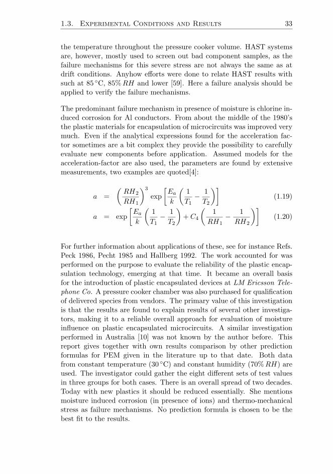
The predominant failure mechanism in presence of moisture is chlorine in-duced corrosion for Al conductors. From about the middle of the 1980’sthe plastic materials for encapsulation of microcircuits was improved verymuch. Even if the analytical expressions found for the acceleration fac-tor sometimes are a bit complex they provide the possibility to carefullyevaluate new components before application. Assumed models for theacceleration-factor are also used, the parameters are found by extensivemeasurements, two examples are quoted[4]:

a =(RH2

RH1

)3

exp[Ea

k

(1T1− 1T2

)](1.19)

a = exp[Ea

k

(1T1− 1T2

)+ C4

(1

RH1− 1RH2

)](1.20)

For further information about applications of these, see for instance Refs.Peck 1986, Pecht 1985 and Hallberg 1992. The work accounted for wasperformed on the purpose to evaluate the reliability of the plastic encap-sulation technology, emerging at that time. It became an overall basisfor the introduction of plastic encapsulated devices at LM Ericsson Tele-phone Co. A pressure cooker chamber was also purchased for qualificationof delivered species from vendors. The primary value of this investigationis that the results are found to explain results of several other investiga-tors, making it to a reliable overall approach for evaluation of moistureinfluence on plastic encapsulated microcircuits. A similar investigationperformed in Australia [10] was not known by the author before. Thisreport gives together with own results comparison by other predictionformulas for PEM given in the literature up to that date. Both datafrom constant temperature (30 C) and constant humidity (70%RH) areused. The investigator could gather the eight different sets of test valuesin three groups for both cases. There is an overall spread of two decades.Today with new plastics it should be reduced essentially. She mentionsmoisture induced corrosion (in presence of ions) and thermo-mechanicalstress as failure mechanisms. No prediction formula is chosen to be thebest fit to the results.


In Refs. [5, 6, 9, 10, 16, 17, 19, 23, 24, 49, 53, 55, 61, 66, 77] the mainoutcomes are with few exceptions the same as before. A few commentscan be done. Brown et al. present IR-microscopy as a non-destructivefailure analysis method, very suitable for plastic encapsulated modules(PEMs) [5]. Acoustic microscopy can be used in a similar way. Nachbauerhas investigated complementary MOS (CMOS) and high-speed CMOS(HCMOS) devices in a pressure cooker at different temperature-humidity-biased (THB) conditions [53]. He preferably uses standard 85 C/85%RHand compares with 132.9 C/85%RH at a bias of 6 V. The results areinterpreted with Weibull plots. Other conditions were also tried. Besidecorrosion parameter shifts are considered as failures. Main conclusionwas that the second test type should be used to accelerate the tests. Stillhigher temperatures are not to recommend as new failure mechanismscan appear. There are two categories of failures:

1. parametric failures, as supply current leakage due to activated par-asitic transistors or source-drain leakage in n-channels

2. complete failures due to corrosion or excessive leakage

Fokkens and Lous performed accelerated moister tests with a CMOS de-vice [17]. The intention was to verify if different pre-treatments as solderdipping and/or thermal cycling could accelerate failure appearance com-pared with untreated parts. The onset of corrosion and electrical degra-dation was determined. They applied a HAST test at 130 C/85%RH,considered as most useful. Pre-treating did not appreciably accelerate thetests.

Matthai has given a second report on THB-tests [49]. He derives equationsfor moisture diffusion in plastics and points out the importance of the glasstransition temperature, TG, at which glassification of the plastics occursand discusses factors influencing it. He applies his model approach totests of bipolar transistors, using Weibull plots for interpretation of testvalues. As most important failure mechanisms the following are observed:

1. Formation of electrolytic distances on the chip surface followed byleakage currents.

2. Corrosion of Al inside the devices causing interruptions of electricconnections.


The report is a rather thorough record of problems involved in reliabilityevaluation of PEMs. Nguyen et al. used for CMOS-devices thermal cy-cling as −65 C/150 C, −40 C/125 C, 0 C/125 C with 2000 cycles [55].Effects of different die coating was registered. Acoustic micrographs il-lustrate moisture attacks in failed parts causing interfacial delamination.A preconditioning by 30 cycles −65 C/150 C bake at 125 C for eighthours, H2O soak and solder reflow were applied. Emerson et al. evalu-ated plastic assemble processes for high reliability applications [16]. Testchips were tried in HAST experiments at 140 C/85%RH and 40 V biasfor different epoxy encapsulants, in one case silicone gel coating. In thefailure distribution an extrinsic region, the curve having a low slope, andan intrinsic region, the curve having a steep slope appeared. The first isassociated with random failures, produced by defects introduced at themanufacturing process. The second region also called wear-out regionis due to failures tied to process or reaction from the material and theenvironment. The overall distribution had a log-normal shape.

Burger investigated the bond-strength (adhesion) of different interfacesin PEMs and developed a test method for this [6]. The componentswere first constrained by usual treatments (HAST, pressure-cooker solderdips, temperature cycling). He presented a mechanical model to describethe corrosion phenomena from pressure cooker tests and temperature cy-cling. Failures were documented by scanning electron microscope (SEM).Scanning Acoustic Microscopy reveals delaminations along the interfaces.Gallo and Munamarty introduced a new failure mechanism for PEMs,popcorning [19]. Character and consequences can be summarized as fol-lows. The failure occurs when the inherently hygroscopic encapsulant israpidly exposed to high temperatures during reflow solder assembly ofthe component to a printed circuit card. The moisture absorbed by themolding compound vaporizes and rapidly expands leading to developmentof high stresses. When these exceed both the interfacial strength and thefracture toughness of the molding compound, delamination and crackingappear. Cracking is accompanied by a characteristic pop sound. Fromthis comes the name popcorning. The phenomenon can lead to a longterm reliability problem, since the cracks can be a path for ionic contam-inants, causing corrosion-induced failures. Another result can be shearedor cratered ball bonds, causing electrical failures.

Schuddeboom and Wuebbenhorst discuss extrapolation to lower temper-ature of results from PEM high temperature storage life (HTSL) [66].They use a model constructed to describe ball-bond corrosion in HTSLstress testing. In this model ion mobility is considered to be the rate


determining step and found to be non-linear for anti-popcorn plastic. AnArrhenius type extrapolation of the meantime to failure (MTTF) at hightemperature is used to predict the value at lower temperatures. Themethod seems to be correct for a low-stress plastic However it, possibly,underestimates the value for anti-popcorn plastic based on ion conduc-tivity data. Strikingly, below the glass-transition of anti-popcorn plastic,the reaction rates estimated from the ion conductivity data are the samefor both the low-stress and the anti-popcorn encapsulants.

Casanovas and White investigated the effect of uncontrolled storage ofPEMs used in naval aviation applications [9]. The presumption is that ifold parts have not degraded after 20 or 30 years of uncontrolled long-termdormant storage, then vastly superior current products will survive sim-ilar periods under similar conditions. Results from destructive physicalanalysis revealed that only two PEMs, both 28 years old, exhibited cor-rosion. Regardless of age, C-mode scanning acoustic microscopy (SAM)revealed delaminated areas in most parts, suggesting that this techniquemight not be a good method for screening PEMs. No direct relationshipwas found between corrosion and moisture content. In addition, oxygenplasma etching was found to be a very effective method for performingdestructive physical analysis on PEMs. The purpose of the evaluationwas to determine if long-term dormant storage affects the reliability ofPEMs for naval aviation applications that demand very high reliability ofthe components. A seven step test flow was developed:

1. External visual inspection

2. Radiographic inspection

3. Electrical testing at room, rated-high, and rated-low temperatures

4. Moisture content (as measured by weight change after a high tem-perature bake)

5. Electrical retest (for any part rejected at step 3)

6. C-mode SAM

7. Destructive physical analysis

From the age distribution of evaluated parts an average lifetime of 16 yearswas found. The leading failure modes were lead finish damage (27 cases),twisted leads (23 cases) and contamination from unknown sources (12


cases). Uno et al. penetrated the thermal reliability problem with gold-aluminium bonds in PEMs [77]. They concentrated on bi-phenyl resin en-capsulants. Bond degradation of gold wires connected to aluminum padshas become a major problem because of the use of molding resins with lowthermal stability and the use of IC devices under high thermal environ-ments. Failures are caused by corrosion reaction of Au-Al intermetallicswith bromine contained as flame retardent in the resin compounds. Itwas clarified that the reactive intermetallic was the Au4Al-phase formedin the bond interface. Typical bond failures would be degradation of bondstrength as well as an increase in electrical resistance. Shear strength andresistance were measured at 473 K. Considerable change of the two pa-rameters occurred. Corrosion reaction at the Au-Al bonds increased theresistivity. Shear strength decreased of corrosion at the gold/intermetallicinterface. The cumulative failure function was interpreted by Weibull andArrhenius plots. Activation energies for the latter were 1.8 eV and 0.6 eVfor bi-phenyl resin and 2.8 eV for O-Cresole Novolac-resin (OCN). Halo-genes are often present in molding compounds and possible reactions withgold and aluminium are shown. Oxygen can also interact. The failureprocess could be divided into several steps:

1. resin decomposition

2. bromine diffusion

3. intermetallic formation

4. chemical reactions

The strength of high purity gold wires and such with impurities werecompared. Alloyed gold bonds are stronger than pure gold bonds. Seealso Uno and Tatsumi [76].

Ranade et al. used a Scanning Acoustic Microscope to reveal False Heal-ing in PEMs [61]. This phenomenon is related to occasionally observedreduction of delamination in PEMs. Previously “false-healing” was re-ported only for the leadframe/plastic interface. It was thought that thechemical contaminants present in the flux enter the package and formcorrosive products which fill up the internal air gaps. The authors madesome new findings for the occurrence of false healing by using acousticmicroscopy. They found false healing in instances where there was noexposure to corrosive media. Additionally false healing was observed atthe die/plastic interface, where chemical contaminants could not reach.


In this study SAM was used to conduct nondestructive evaluation of pack-ages subjected to preconditioning and simulated assembly processes. Theresults indicate two major questions in the previous false healing theory.First, the theory cannot explain the occurrence of false healing at theleadframe/plastic interface in situations where there was no exposure tocorrosive flux and the recovery of delamination at the die/plastic inter-face where chemical contaminants cannot reach. A new explanation iswarranted to explain these findings. One explanation for the reduction indelamination could be that the baking drives residual moisture (presentafter IR reflow procedure) out of the encapsulant allowing it to adhereback with the die and lead frame. This could be confirmed by some ex-periments. Moisture inside the package is responsible for showing up asdelamination.

Swanson et al. used different methods to evaluate PEMs for militaryuse [72]. Instead of conventional parts they applied special moisture andstress sensor chips in single PEMs. Temperature cycling, THB, HASTand high temperature storage/operating life (HTOL) tests were applied.Device reliability tests were performed on single test devices using the sil-ver comb pattern sensor, the NiCr resistor consisting of an unpassivatedNiCr resistor network and the Sandia ATCO4 chip that has an array ofpiezo resistors, thermal heaters and temperature diodes. A conventionalhermeticity screening is required to provide confidence test when usingPEMs. Sample ICs were assembled on leadframes, transfer molded andthe exposed to a series of environmental screens. One device, a silver-comb pattern sensor provides a go/no-go test. The NiCr resistor providesa more quantitative indication of moisture at the interface.

Epoxy encapsulants, unlike silicones, are not chemisorbed onto the die andslight shrinkage combined with diffusion allows moisture accumulation.As to moisture sensors no failures were found after 24 and 100 hours ofHAST and 24, 168, 500 and 1000 hours of 85 C/85%RH HTOL. ForNiCr resistor changes in thermal 500 times cycling were less than 10%for all parts. All parts in HTOL showed less than 5% change at 125 Cfor 1000 hours except one (at no bias). In another 85 C/85%RH testingwithout bias one part had an opening but all changes were below 5%.No openings or significant change in HAST parts (bias or no bias) werefound. Many other test results are given in the report.

Hakim came early with objections to the use of the Arrhenius plot indetermining failure rates [23, 24]. First he meant that temperature wasnot the crucial cause for failures but misfits of the components in their


electrical environment on system level. As to humidity attacks in PEMshe says that corrosion is not any more a failure mechanism of concernfor the user. This should be due to material and design improvements ofPEMs.

He suggests the same tests as for hermetic encapsulants. We have heretwo definitions of reliability. Evidently component failure rate on systemlevel can be different from that in individual component tests. But thelatter is necessary for the certification of the component. The vendor doesnot know in which environment his component will be used. The PEMsare of course subject to other failures than corrosion as the tests describedabove demonstrate and should be tried for that. Hakim also refers mostlyto components for military use. He mentions that MIL-HDBK-217 is notused any more as being uncertain. But this is due to its vast applicabilityto different environments, benign and harsh for instance. It includes also ahuman factor as often elderly people not specialized in electronics handleadvanced equipments. This handbook should be used only for militaryapplications. Quality experts often recommend Bell Lab (AT&T) modelsfor telecom applications. In Europe similar handbooks were published inGreat Britain, France and Italy.

Aluminum corrosion is still to be regarded as an important failure mech-anism. Hakim helped Reich in his pioneering work on moisture influencein PEMs [62]. Charles mentions also vapour pressure models [10]. Theyshow good correlation between results below 100 C, but are less satisfac-tory for the more accelerated tests and have fallen in disfavor. Gunn etal. tested devices at the same vapor pressure, but differing temperaturesand humidities and concluded that the device lifetime was not a simplefunction of vapor pressure or vapor pressure in conjunction with tem-perature [21]. Charles also makes difference between results interpretedwith constant activation energy, Ea, and those with humidity dependentenergy. The latter was confirmed in this thesis to be more consistentwith experimental results. Anyhow, ion induced corrosion is not yet anabandoned failure mechanism. Traditional statistic process control (SPC)should be used for PEMs as well. This control means that a compound isfollowed when in use and failure rates recorded and stored in a computer.An increase in rate gives an alarm. The failed parts are investigated bythe user and/or the vendor. The fault in the production is traced andcorrected.

Earlier tests were mentioned for high reliability purposes. A 2-chambersystem with high temperature (100 C) in one of them and low tempera-


ture (−10 C or so) in the other with a lift carrier for rapid change betweenthem. Then most test possibilities are given. the corresponding ESD testswill be treated in next chapter.

As reliability tests are expensive and time consuming a major goal for fu-ture work will be to found out which tests can be discarded for new highquality microcircuits. As seen from the diagrams on surface conductiv-ity (or resistivity) they converge often to a point or small area near 0 C(273 K) where most water is in the solid phase. Contamination, however,can give a lower freezing point. This is in agreement with the physical lawsof thermodynamics, what supports the approach. There is no distinct dif-ference in moisture resistance between discrete components and very largescale integration (VLSI)-circuits. At low temperature/humidity tests (e.g.85 C/85%RH) the contact pads are first being attacked, while at HASTconditions also the narrow conductor stripes are damaged. Discrete partshaving larger dimensions should be more resistive against humidity con-straints.

A generally applied method to improve the reliability of vendor compo-nents is the burn-in process. The devices undergo dynamic tests at ele-vated temperature and humidity condition for a rather short time (from24 hours to several days). Thus weak parts are eliminated in advance,compare also with the HAST procedure. By applying surface protectionthe influence of moisture is reduced, but this is also a matter of cost. Aproper encapsulation is important. The properties of plastic encapsula-tion material has been significantly improved during the last two decades.

1.3.2 An Example of Evaluation of Accelerated Tests

When testing components at some temperature, T, the failures will havesome distribution in time. This depends upon the failure mechanisms,represented by their activation energies, Ea and the temperature. Thelog-normal distribution has been found to be common for electronic com-ponents. Assuming a normalized log-normal distribution the followingdeduction for comparison of failure distributions at different temperaturescan be done. The failure rate at a certain time, t, will be:

λ(t) = λ0(t)(−Ea

kT

)(1.21)


But the failure intensity is defined:

Z(t) =f(t)R(t)

thenf(t)R(t)

= λ0(t) e−Ea/kT . (1.22)

R is called the reliability function. The mean life-time τ , however, isdefined as follows:

τ = MTTF =

∞∫0

R(t) dt = e−Ea/kT

∞∫0

f(t)λ0(t)

dt (1.23)

For two temperatures TA and TB there is:

τ(TA)τ(TB)

= exp[Ea

k

(1TA− 1TB

)](1.24)

In the same way at each time point, t, with a certain failure outcome ∆f,this is transformed. Compare distribution according to scale, A, with thatof scale, B, in Fig. 1.49. If the variance, σ, of the log-normal distributionis given it is easy to calculate the time span to a certain percentage failureoutcome, x, compared to tm (time to 50% outcome). Other distributionfunctions in time will need different approaches. Another rather commondistribution for the failure of components is the Weibull distribution.Because the following holds for the log-normal distribution of failures,F (t) up to time t is:

F (t) =12

[1 + erf

1√2σ

ln(t

tm

)] (1.25)

The error function erf is defined as:

erf(Y ) =2√π

Y∫0

e−n2dn (1.26)

The function F is numerically given in Ref. 56, for instance. Some valuesfor σ = 0 are given in Table 1.6:

One way to formally extend the expression for a log-normal failure dis-tribution to include the temperature according to the Arrhenius plot is a


Table 1.6: Numerical values of thefailure function F (t) for σ = 1.

F (t) t/tm

0.2 0.430.5 1.000.8 2.320.9 3.601.0 > 96.34

transformation of the time scale:

t −→ t eEa/kT1 = t1 (1.27)t −→ t eEa/kT2 = t2 (1.28)

t1t2

= eEa/k(1/T1−1/T2) (1.29)

For T −→ ∞ the fictive time t1 approaches t. A direct transformationbetween two arbitrary temperatures T1 and T2 is also possible:

t1 −→ t2 exp[Ea

k

(1T1− 1T2

)](1.30)

We make the following definitions:

f(t) the probability density function, failure density

F (t) the probability distribution function, failure distribution

R(t) the reliability function

Z(t) the probability intensity function, failure intensity

The failure density without transformation is

f(t) =1

tσ√

2πexp

[− 1

2σ2

ln(t

tm

)2]

(1.31)


Thus:

f(t) → f(t eEa/kT

)=e−Ea/kT

tσ√

2π

× exp

− 1σ2

ln

(t eEa/kT

tm eEa/kT

)2(1.32)

f(t)dt → f(t eEa/kT

)dt eEa/kT (1.33)

and

∞∫0

f(t)dt =

∞∫0

f(t eEa/kT

)dt eEa/kT (1.34)

=

∞∫0

e−Ea/kT

tσ√

2πexp

[− 1

2σ2

ln(t

tm

)2]dt eEa/kT

= 1 (1.35)

likewise:

F(t eEa/kT

)=

12

[1 + erf

1√2σ

ln

(t eEa/kT

tm eEa/kT

)]

(1.36)

this means that F (t) is invariable. Also R(t) is invariable under thistransformation:

R(t) = 1− F (t) = 1− F (t eEa/kT ) = R(t eEa/kT ). (1.37)

The failure intensity Z(t) transforms as

Z(t) =f(t)R(t)

= λ0(t) (1.38)

Z(t eEa/kT ) =f(t eEa/kT

)R(t eEa/kT

)=

e−Ea/kT f(t)R(t)

. (1.39)

Finally we findZ(t eEa/kT ) = e−Ea/kT λ0(t). (1.40)


Figure 1.49: Time displacement of failure outcome at accelerated tests. Thesame time scale is valid for A and B with TA = 50 C and TB = 100 C.

The physical validity of the transformation is, however, not proven by theequations above alone. But the requirements of the reliability functionsf(t), F (t), R(t) and Z(t) are fulfilled, anyhow, and the transformationagrees with experiments.


Table 1.7: Accelerated Testing Evaluation (From MIL-STD-883).

Failure Type Activation Detection Preventive

Mechanism Energy Ea Measure

Slow trapping wearout 1.0 eV High temp.bias

Ultra-cleanprocessing

Contamination wearout/ infant

1.4 eV High temp.bias


Surface charge wearout 0.5−1.0 eV

High temp.bias


Aluminum elec-tromigration

wearout 0.5−1.0 eV

High temp.operating life

Limitedcurrentdensity inconductors

Microcracks random — temp. cycling Contouredoxide steps

Contracts wearout — High temp.operating lifeand stress


Oxide defects infant 0.3 eV High voltageoperating lifeand stress


Ion migration wearout 1.4 eV High temp.bias


Corrosion random 0.3−0.6 eV



Au-Alintermetallicbond failures

random /wearout

1.02−1.04 eV


Minimizesuch bonds

Surfaceinversion

random 1.02 eV High temp.bias


Moisturerelated

random — Cold temp.near dewpoint

Dry sealing


1.4 References

[1] Ansorge, F.; Becker, K. F.; Ehrlich, R.; Azdasht, G.; Bader, V.; Aschenbrenner,R. and Reichl, H.Recent progress in flexible molding and reliability investigation of CSP and BGA-packages using advanced interconnection technology.In Proceedings IEEE Int. Symp. on Polymeric electronics packaging, PEP’97 (NewYork), pp. 14–22 (1997).

[2] Awakuni, Y. and Calderwood, J. H.Water vapor adsorption and surface conductivity in solids.Journal of Physics D: Applied Physics, vol. 5 (5), pp. 1038–1045 (1972).

[3] Bickley, J.Boitiers ceramique ou plastique: quelle est leur fiabilite?Electronique Industrielle, vol. 9, pp. 37–39 (1981).

[4] Birolini, A.Reliability Engineering: Theory and Practice (Springer Verlag), 4th edn. (2003).

[5] Brown, J.; Footner, P. K. and Richards, B. P.Failure analysis of plastic encapsulated components - the advantage of IR mi-croscopy.Journal of Microscoscopy, vol. 148 (2), pp. 179–194 (1987).

[6] Burger, K.Fracture mechanical characterization of IC-device interfaces.Quality and Reliability Engineering International, vol. 11 (4), pp. 299–305 (1995).

[7] Burgess, J. F. and Yerman, A. J.Accelerated corrosion tresting in pressure cooker at 130 C.In Proceedings ECC Conference. pp. 119–126 (1986).

[8] Burggraaf, P. S.Semiconductor plastic encapsulants: Moulding components.Semiconductor International, vol. 3 (9), pp. 47–64 (1980).

[9] Casanovas, A. and White, J. W.Commercial plastic encapsulated microcircuits for Naval aviation applications.Application Technical Digest 1, Johns Hopkins (1997).

[10] Charles, S.The reliability of plastic encapsulated integrated circuits in humid environments.Australian Telecommunication Research, vol. 20 (2), pp. 39–50 (1986).

[11] Choi, K.-S.; Kang, D.-S.; Cho, J.-W. and Kim, Y.-G.Environmentally reliable plastic design for the charge-coupled device (CCD).In Proceedings ISHM’96. pp. 254–258 (1996).

[12] Christou, A. and Wilkins, W.Assessment of silicone encapsulation materials: Screening technique.In Reliability Physics 15th Annual Proceedings - 1977 (IEEE), p. 112 (1977).

1.4. References 47

[13] Christou, J. R., A. Griffith and Wilkins, B. R.Reliability of hybrid encapsulation based on fluorinated polymeric materials.IEEE Transactions on Electron Devices, vol. ED-26 (1), pp. 77–83 (1979).

[14] Conn, T.; Eachus, J.; Klema, J.; Pyle, R. and Schwiesow, B.Moisture resistance testing of packages.Semiconductor International, vol. 11 (2), pp. 80–81 (1988).

[15] Dwight, H. B.Mathematical Tables of Elementary and some Higher Mathematical Functions(Dover Publications, New York), 3rd edn. (1961).

[16] Emerson, J. A.; Sweet, J. N. and Peterson, D. W.Evaluating plastic assembly processes for high reliability applications using HASTand assembly test chips.In Proceedings Electronic Components and Technology Conference. pp. 191–195(1994).

[17] Fokkens, K. and Lous, A.Comparing HAST results of differently pretreated plastic encapsulated integratedcircuits.Microelectronics and Reliability, vol. 29 (6), pp. 1003–1009 (1989).

[18] Gallo, A. A.Effect of mold compound components on moisture-induced degradation of gold-aluminum bonds in epoxy encapsulated devices.In Proceedings IPRS. pp. 244–251 (1990).

[19] Gallo, A. A. and Munamarty, R.Popcorning: A failure mechanism in microcircuits.IEEE Transactions on Reliability, vol. 44 (3), pp. 362–367 (1995).

[20] Guan, D. Y.; Gukelberger, T. F.; Cahoon, E. C.; Joseph, T. W. and Snowdon,J. M.New failure mechanisms in temperature and humidity stress.In 36th Electronic Components Conference Proceedings 1986 (New York), pp. 107–110 (1986).

[21] Gunn, J. E.; Malik, S. K. and Mazumdar, P. M.Highly accelerated temperature and humidity stress test technique (HAST).In Reliability Physics 19th Annual Proceedings - 1981 (IEEE), pp. 48–51 (1981).

[22] Gustafsson, K. and Lindborg, U.Chlorine content in and life of plastic encapsulated microcircuits.In Proceedings — Electronic Components Conference. pp. 491–499 (1987).

[23] Hakim, E. B.Plastic encapsulated microcircuit reliability prediction, why?Microelectronics and Reliability, vol. 38 (4), pp. 681–683 (1998).

[24] Hakim, E. B.Do we need a PEM reliability model?Quality and Reliability Engineering International, vol. 15, pp. 283–286 (1999).


[25] Hallberg, O.Humidity accelerations for testing standards.In Proceedings ESREF 92. pp. 331–334 (1992).

[26] Hasegawa, T. and Shibuya, Y.Photoelasticity analysis of thermal stresses in the plastic ICs.Transactions of the Institute of Electrical Engineers of Japan, vol. 112-A (10), pp.866–873 (1992).

[27] Hellstrom, S.Environment testing of plastic encapsulated cross point thyristors with ceramicencapsulated as comparison (1978-1979).Internal Report 7280/X/Ag 4238, LM Ericsson.In Swedish (1978–1979).

[28] Hellstrom, S.Determination of acceleration factors for the test of plastic encapsulated ICs bymeasuring the surface conductivity.Internal Report 7250/X/Ag 2156, LM Ericsson.In Swedish (1980).

[29] Hellstrom, S.On the choice of component sampling, the meaning of AQL (Acceptable QualityLevel) and AOQL (Average Outgoing Quality Limit) and the distribution of failureoutcome at temperature accelerated tests.Internal Report 70 201/X/ag 2129, LM Ericsson.In Swedish (1980).

[30] Hellstrom, S.On the method of obtaining acceleration factors from surface conductivity mea-surements.Internal Report 7250/X/Ag 3016, LM Ericsson (1980).

[31] Hellstrom, S.On the choice of an average activation energy for LSI-device reliability evaluation.Internal Report 7280/XK/Ag 4324, LM Ericsson (1981).

[32] Hellstrom, S.Surface conductivity measurements (I).Internal Report XT/HG 1539, LM Ericsson (1984).

[33] Hellstrom, S.Surface conductivity measurements (II).Internal Report XT/HG 1608, LM Ericsson (1984).

[34] Iannuzzi, M.Development and evaluation of a preencapsulation cleaning process to improvereliability of HIC’s with aluminum metallized chips.IEEE Transactions on Components, Hybrids and Manufacturing Technology, vol.CHMT-4 (4), pp. 429–438 (1981).

[35] Iannuzzi, M.Bias humidity performance and failure mechanisms of new hermetic aluminumSIC’s in an environment contaminated with Cl2.

1.4. References 49

In Reliability Physics 20th Annual Proceedings - 1982 (IEEE), pp. 16–26 (1982).

[36] Iannuzzi, M.Reliability and failure mechanisms of non- hermetic aluminum SIC´s: Literaturereview and bias humidity performance.IEEE Transactions on Components, Hybrids and Manufacturing Technology, vol.CHMT-6 (2), pp. 181–190 (1983).

[37] Johnson, B. and Verma, V.Reliability assessment of fielded plastic and hermetically packaged microelectronics.IEEE Transactions on Reliability, vol. 45 (1), pp. 23–26 (1966).

[38] Koelsman, H.Metallization corrosion in silicon devices by moisture-induced electrolysis.In Reliability Physics 12th Annual Proceedings - 1974 (IEEE), p. 168 (1974).

[39] Kolesar, S. C.Principle of corrosion.In Reliability Physics 12th Annual Proceedings - 1974 (IEEE), p. 155 (1974).

[40] Labuda, E. F.The unform gold process — A metal pattern generation technique for integratedcircuits with beam lead metallization system.In Spring Meeting Electrochemical Society - Extended Abstracts. p. 195 (1974).

[41] Lawson, R. W.The qualification approval of plastic encapsulated semiconductor components foruse in moist environments.In Proceedings Symp. on plastic encapsulated semiconductor devices (RSRE, UK).Paper 7 (1976).

[42] Lin, R.; Blackshear, E. and Serisky, P.Moisture induced package cracking in plastic encapsulated surface mount compo-nents during solder reflow process.In Reliability Physics 26th Annual Proceedings - 1988 (IEEE), pp. 83–89 (1988).

[43] Lowry, R. K.; Hanley, K. L.; Hatcher, J.; Gu, X.; Julien, N. and Astrab, D.Plastic encapulant materials consistency for reliability assurance.In Proceedings ISTFA’95. pp. 101–109 (1995).

[44] Lycoudes, N. E.The reliability of plastic microcircuits in moist environment.Solid State Technology, vol. 21 (10), pp. 53–62 (1978).

[45] Malik, S. K.; Gunn, J. E. and Camenga, R. E.Future of temperature and humidity testing: Highly accelerated temperature andhumidity stress test (HAST).In Proceedings International Test Conference (Philadelphia, USA), pp. 790–795(1983).

[46] Manchester, K. E.; Bird, D. W. and Charest, H.A contribution of polymer die attach systems to the reliability of plastic encapsu-lated integrated circuits.In Reliability Physics 20th Annual Proceedings - 1986 (IEEE), pp. 272–275 (1982).


[47] Mancke, R. G.A moisture protection screening test for hybrid circuit encapsulants.IEEE Transactions on Components, Hybrids and Manufacturing Technology, vol.CHMT-4 (4), pp. 492–498 (1981).

[48] Matthai, G.A model for mechanisms in plastic encapsulated microelectronic devices duringtemperature-humidity tests - I.Microelectronics and Reliability, vol. 30 (5), pp. 835–838 (1990).

[49] Matthai, G.A model for mechanisms in plastic encapsulated microelectronic devices duringtemperature-humidity tests - II.Microelectronics and Reliability, vol. 31 (5), pp. 873–878 (1991).

[50] Mei, Y.; Liu, S. and Suhir, E.A parametric study of a VLSI plastic package subjected to encapsulation, moistureabsorption and solder reflow process.In Structural Analysis in Microelectronic and Fiber Optic Systems. vol. 12 of Amer-ican Society of Mechanical Engineers, EEP, pp. 159–174 (1995).

[51] MIL-STD-105D: Sampling procedures and tables for inspection by attributes.Military Standard.US department of defense (1963).

[52] MIL-STD-414: Sampling procedures and tables for inspection by variables for per-cent defective.Military Standard.US department of defense (1957).

[53] Nachbauer, W.Highly accelerated humidity testing of CMOS ICs.Electronic Components & Applications, vol. 8 (3), pp. 156–166 (1988).

[54] Nallino, M.; Digout, R.; Deleuze, G. and Brizoux, M.Plastic encapsulated ICs reliability prediction modelling: Principal results.In Proceedings ESREF’92. pp. 311–321 (1992).

[55] Nguyen, L. T.; Gee, S. A.; R., J. M.; Grimm, H. E.; Berardi, H. and Walberg,R. L.Effects of die coating, mold compounds and test conditions on temperature cyclingfailures.In Proceedings Electronic Components and Technology Conference. pp. 210–217(1994).

[56] Ogawa, K.; Suzuki, J. and Sano, K.Automatically controlled 2-vessel pressure-cooker test-equipment.IEEE Transactions on Reliability, vol. R-32 (2), pp. 164–167 (1983).

[57] Olsson, C.Reliability of plastic-encapsulated logic circuits.Quality and Reliability Engineering International, vol. 5 (1), pp. 53–72 (1989).

1.4. References 51

[58] Pecht, M.; Nyguen, L. and Hakim, E.Plastic encapsulated microcircuits (John Wiley & Sons) (1995).

[59] Peck, D. S.Comprehensive model for humidity testing correlation.In Reliability Physics 24th Annual Proceedings - 1986 (IEEE), pp. 44–50 (1986).

[60] Ramsey, T. H.Aluminum alloy bonding wires in corrosive environments.Semiconductor International, vol. 10 (4), pp. 90–94 (1987).

[61] Ranade, Y.; Pecht, M. G. and Moore, T. M.New findings in the occurrence of false-healing in plastic encapsulated microcircuitsusing Scanning Acoustic Microscopy.IEEE Transactions on Components and Packaging Technologies, vol. 22 (2), pp.266–299 (1999).

[62] Reich, B.Acceleration factors for plastic encapsulated semiconductor devices and their rela-tionship to field performance.Microelectronics and Reliability, vol. 14, pp. 63–66 (1975).

[63] Reich, B.Bias influence on corrosion of plastic encapsulated device metal systems.IEEE Transactions on Reliability, vol. R-25 (5), pp. 296–298 (1976).

[64] Roberts, B. C.Plastic encapsulation of semiconductor devices.In Int. Conf. Plastics in Telecommunication 3, Programme and Papers (London)(1982).

[65] Sbar, N. L. and Kozakiewicz, R. P.New acceleration factors for temperature, humidity, bias testing.IEEE Transactions on Electron Devices, vol. ED-26 (1), pp. 56–71 (1979).

[66] Schuddeboom, W. and Wuebbenhorst, M.Question marks to the extrapolation to lower temperatures in high temperaturestorage life (HTSL) testing in plastic encapsulated ICs.Microelectronics and Reliability, vol. 36 (11/12), pp. 1935–1938 (1996).

[67] Sim, S. P. and Lawson, R. W.The influence of plastic encapsulants and passivation layers on the corrosion ofthin aluminium films subjected to humidity stress.In Reliability Physics 12th Annual Proceedings - 1974 (IEEE), pp. 103–112 (1974).

[68] Sinnadurai, F. N.The accelerated ageing of semiconductor devices in environments containing a highvapor pressure of water.Microelectronics and Reliability, vol. 13, pp. 23–27 (1974).

[69] Sinnadurai, N.EPIC: A Cost-effective plastic chip carrier for VLSI packaging.IEEE Transactions on Components, Hybrids and Manufacturing Technology, vol.CHMT-8 (3), pp. 386–390 (1985).


[70] Sinnadurai, N.Plastic packaging is highly reliable.IEEE Transactions on Reliability, vol. 45 (2), pp. 184–192 (1996).

[71] Stroehle, D.Plastic encapsulated semiconductor components for telecommunication systems.Electrical Communication, vol. 57 (2), pp. 152–156 (1982).

[72] Swanson, D. W.; Chen, M. and Enlow, L. R.Evaluation of moisture and stress sensor chips in single-chip PEMs, temperaturecycling, THB, HAST, and High-Temperature storage / operating life tests.In Int. Symp. on Microelectronics 1999. pp. 233–239 (1999).

[73] Terasaka, K.; Tsujii, Y.; Hitsui, N.; Amari, Y.; Kakimoto, T.; Yamazaki, T. andTakezaki, T.Accelerated testing of moisture induced aluminum corrosion.In Reliability Physics 22th Annual Proceedings - 1984 (IEEE), pp. 458–462 (1984).

[74] Torii, M.; Kagawa, H. and Kyotani, H.Highly reliable packaging material for VLSI.Technical Report 37, Matsushita-Electric.In Japanese (1988).

[75] Tsubosaki, K.; Wakashima, Y. and Nagasima, N.Rate determining factor of aluminum corrosion and a rapid method of assessingthe moisture resistance of LSI PEMs.In Reliability Physics 21th Annual Proceedings - 1983 (IEEE), pp. 83–89 (1983).

[76] Uno, T. and Tatsumi, K.Thermal reliability of gold-aluminium bonds biphenyl epoxy resin.Microelectronics and Reliability, vol. 40, pp. 145–153 (2000).

[77] Uno, T.; Terashima, S.; Onoue, K. and Tatsumi, K.Improvement in thermal reliability in gold-aluminium bonds encapsulated in bi-phenyl epoxy resin.In Int. Symp. on Microelectronics 1998. pp. 591–596 (1998).

[78] Wada, T.; Kobayashi, Y.; Maeda, M.; Sugimoto, M. and Ajiki, J.Study of acceleration factor on moisture resistance test of plastic encapsulatedsemiconductor devices.Microelectronics and Reliability, vol. 28 (5), pp. 813–820 (1988).

[79] Walter, H.; Schroen, J. L.; Spencer, J. A.; Bryan, J. A.; Cleveland, R. D.; Metzgar,T. D. and Edwards, D. R.Reliability tests and stress in PECs.In Reliability Physics 19th Annual Proceedings - 1981 (IEEE), pp. 81–87 (1981).

[80] Wilson, K. J.; Henderson, J. C. and Sutherland, R. R.Some problems in the correct failure analysis of plastic encapsulated semiconductordevices.In 36th Electronic Components Conference Proceedings 1986 (New York), pp. 132–137 (1986).

1.4. References 53

[81] Yoshida, T.; Takahashi, T. and Koyama, S.A new accelerated test method for moisture resistance of large scale PEMs.In Reliability Physics 20th Annual Proceedings - 1982 (IEEE), pp. 268–271 (1982).

2ESD Investigations

2.1 Introduction

Charging of matter is a very old phenomenon. Already in ancient Greeceit was discovered, that amber when rubbed in some way attracted smallparticles. This was later recognized as an effect of electrical charges onthe surface of the amber material. The word electricity comes from theGreek name of amber, electron. After this first manifestation of electricitya more precise study did come only after many centuries. The rubbingprocess to form static electricity was denoted triboelectric charging afterthe Greek word tribein = rubbing, frictioning. It was also realized thattwo kinds of static electricity were created. One came to be called positivethe other negative and the last one identified as electrons, an elementaryparticle defined in modern atomic physics. The positive part were atoms,that had lost one or more orbital electrons, i.e. ions. If two differentmaterials are kept close to each other and than suddenly separated orthe two materials are rubbed against each other, one of them will bepositively and the other negatively charged. The last one is said to havethe higher electron affinity. This property of matter is related to thedifferent dielectric constants of the materials. The British physicist andchemist M. Faraday established the so called triboelectric series. This

56 ESD Investigations

is a table of different materials arranged in a manner that materials atthe top are more prone to be positively charged and those at he bottomnegatively. If two materials of the table are separated from each othersor rubbed against each others, the one with higher place in the tablebecomes positively charged, the other negatively charged and the greaterthe distance between them in the table the larger the charge formed.The process depends also upon the properties of the surfaces of the twomaterials, see Table 2.1. Charges of equal sign were found to repel eachother, those of same sign to attract each others. For a short historicalsummary of the “happenings” in electrostatics see the introductory partof [21].

2.2 ESD-Testing and Models

2.2.1 General

In the 1960’s a very high vulnerability of the new discrete MOS-compo-nents was realized. They failed often without any apparent reason. Athorough failure analysis of damaged components started to settle failuremechanisms. This led to the understanding that electrostatic discharge(ESD) caused voltage breakdown in the thin silicon gate oxide of theMOS-circuits. The accidents happened during the handling of the circuits.The operators had been charged triboelectrically and by touching somepin of the circuit a discharge destroyed it. The thickness of the oxideswas normally about 1000 A, corresponding to a breakdown voltage 100V.The failure mode was often a short circuit between gate and source ordrain. About 50% of all failures were caused by ESD.

The failure mechanism clarified preventive measures had to be taken. Allpersonnel handling the circuits in production, control and packing at themanufacturers, respectively unpacking, testing and mounting for use inequipment fabrication by the receiver could harm the circuits. They werecharged in this normal work and caused discharges when handling thecircuits. The results can be, if not catastrophical, that some parametersare changed making the circuit unusable for intended application.

The first action was to protect the MOS-components by keeping them ina metal foil until they were to be mounted. This implied some protectionas the components were shielded against external fields and discharges tothe gate oxide. But hazards remained still at wrapping and unpacking

2.2. ESD-Testing and Models 57

the items, testing and mounting them. The problem was attacked indifferent ways. Protection circuits could be designed and implementedin the component wafer. The first protection circuits had resistors andcapacitors as elements. Experiments were also performed with spark gaps.The function of the protection circuits is twofold, to reduce the pulseheight to a non- dangerous level before the pulse reaches the gate and todissipate the pulse energy in their resistors.

Many investigations started in USA to find out under what circumstancespeople get charged and to which level depending on different activities. Atthe same time a more effective design of protection circuits began. Theybecame faster, withstood more pulse energy and consumed less space onthe wafer. The inputs of the circuit being most sensitive were protectedfirst.

Methods to test the susceptibility of components for ESD came to be con-sidered, including the efficiency of the protection circuits. Modern micro-circuits can sometimes be protected against several thousands volts. Thishas been realized for most CMOS-circuits. Methods for failure analysisof components damaged by ESD were developed. They aimed at localiz-ing the failure site and clarifying the failure mechanism. Being regardedas a big problem for the electronic industry some kind of cooperationto study the ESD-phenomena was felt necessary and a symposium onthe matter was initiated in 1979, the first EOS/ESD-symposium in USA.These could be repeated annually and formed a forum for treating ESD-problems. Around 1500 participants from both USA and Europe andJapan confirms the importance found for dealing with ESD-phenomena.In 1982 the US EOS/ESD-association was established cosponsoring theESD-symposia. EOS means electrostatic overstress and represent theconventional transients.


Figure 2.1: Relationship between charging generators and ESD-testing mod-els.


Figure 2.2: Sketch of the situation to which the Human Body Model applies.The electrostatically charged operator discharges through the external pins intothe chip itself.

2.2.2 Human Body Model

The discharge from operators to electronic circuits described above be-came the background for the first ESD-testing model. On this modelsimulators were constructed to measure the ESD-susceptibility of elec-tronic components. The simulator produces electrical pulses of the sameshape as those from natural discharges. The human body is representedby a capacitor and a series resistor. Because of his capacitance to eartha person can, if insulated, keep this charge until a contact to earth ismade. Metal parts have the function of “local” earth. The human bodyis also able to conduct current, the outer parts of the skin normally area current path and represent a resistor. The value of this resistor will ofcourse vary from person to person. For the Human Body Model (HBM)it was decided to have a capacitance of 100 pF and resistor of 1500 Ω asstandard values. The real capacitance for the human body is of coursealso no constant. Values as high as 500 pF and low as 70 pF have beenmeasured. They are also dependent on the geometric relation of the bodyto earth.

The Human Body Model (HBM) simulation, implying charging a capac-itor and discharging it through a resistor to a component, is a simpli-fication. Both capacitance and resistance are distributed in the bodyand some inductance action of the body occurs. The model should, tobe more correct, include a complicated net of impedances, the magnitude


varying from one person to another. The HBM simulator has, however, re-mained the same for about twenty years. It has become standardized andis described in MIL-STD-883C method 3015.7, “Test Methods and Pro-cedures for Microelectronics”, and the US ESD Ass. standard for HBM.Main characteristics are for the realized pulse a rise-time of less than 10 nsand pulse length of 150 ± 20 ns. This wave form shall be checked usinga current probe and the component socket short circuited. The effectivecapacitance is to be measured by an electrometer. In Notice 7 is alsostipulated a maximum value for so called ringing of the pulse, 15% of theamplitude. Failure criteria for components tested by the HBM-methodcan be:

1. any parameter gets its value moved outside the specification range

2. any parameter value is changed 10% or more after the test

This means that a component whose leakage current exceeds the maxi-mum allowed value after the test is disqualified. If in a test a transistorcurrent amplification factor changes by 10%, the transistor will be disap-proved, even though the factor is still within the specified range. DifferentHBM-simulators can give different test results even if they are of the samemanufacturer. This can be due to only small differences in rise-time orpulse energy, being the crucial conditions for a damage to arrive or not. Astandard HBM circuit for testing is found in Fig. 2.3 and standard pulseshape in Fig. 2.4.

The chosen values of resistor and capacitor correspond, as mentioned,not always to empirical discharge conditions. Experience seems to showthat the resistor value is too high. An absolute value for the ESD sen-sitivity for HBM-discharge is thus difficult to obtain and the method istherefore “mostly used as a reference to compare the sensitivity for differ-ent components”. But today an essential improvement has been gainedfrom the long-term experience. The test equipments have become moresophisticated.

In many commercial HBM ESD-testers the influence of the contributionto the capacitance from the relays has not been sufficiently analyzed. Theeffect can be a 15 − 20% too high capacitance. Inductances of the con-ductors and capacitive interaction between conductors and relay contactswill often affect energy and the discharge time for automatic ESD-testers.According to MIL-STD-883D, method 3015.7 (March 1989), input andoutput of an IC-component shall be tested against all others with five


CCR

R L

CS Rin

++U0 u(t)

DUT

Figure 2.3: An outline of the simple HBM scheme. The capacitor C = 100 pFhas been charged from a high voltage unit. When closing the switch the capacitoris discharged through the resistor R = 1.5 kΩ and inductance L ∼ 5µH into theDUT, represented by CS and Rin. The parasitic capacitance CR can be in theorder of 1 pF. The discharge has passed within about 200 ns. The pulse form ischecked by measuring the current pulse i(t) with the DUT replaced by a currentprobe.

positive and five negative pulses. One second delay between the pulseswill give sufficient cooling. Compare also with the ANSI EOS/ESD S 5.1-1994 standard. All this testing will take at least one hour or in realityabout one working day to manually investigate a 20 pins dual in-line (DIL)package. Fortunately, automatic HBM testers were elaborated in the last10 years making the measuring time much shorter. In the standards thereare detailed descriptions on how to qualify the test equipment and how toperform ESD component tests. All this is necessary to be able to comparemeasured values from different testers.

2.2.3 Machine Model

When components started to be manipulated in machines, such as testingequipments at arrival inspection, automatic mounting robotics in pro-duction and automatic printed circuit board (PCB)-testers by final in-spection, an increase in damages was noted Failure analysis afterwardsrevealed that ESD often was the reason. Many microcircuits that weredestroyed had passed the ESD-test according to HBM method, and yetthey failed. The input protection circuit in general remained intact, al-though the main circuitry was harmed. This indicated a new kind of dis-charges compared to the HBM. Investigation performed in Japan provedthat the component handling equipment generated these very hazardousdischarges. Parts of the testing or measuring equipment became chargedand when pins (connectors) of components came in contact with thema discharge was released damaging the components. From a number of


Figure 2.4: HBM voltage pulse according to MIL-STD-883D. Ringing is al-lowed to be at most 15% of the peak value. The rise-time should not exceed 10 nsas measured between 10% and 90% of the peak value, while the decay time con-stant should be 150 ns as measured between the peak voltage and 1/e = 36.8%of this value.

Figure 2.5: Schematic outline of Machine Model.

measurements a capacitance value of the magnitude 200 pF was found forthe charged equipment parts. The discharge resistances, often metal tometal, proved to be very low, in reality so low that no extra resistor isnecessary in a simulation model. These investigations resulted in a modelwith a discharge circuit consisting of a 200 pF capacitor and a “zero ohm”discharge resistor, named the Machine Model (MM). The discharge pulsesare much faster compared with those of HBM-method. The latter gives apulse time constant of about 0.1µs, while that of Machine Model (MM)is only of the order some tens of nanoseconds. The fast discharge meansthat the protection circuits, effective against HBM pulses do not havetime to react and other protection means must be used.

The Machine Model has the same configuration as the Human BodyModel, only the capacity is 200 pF instead of 100 pF and a serial resis-tance as low as possible. This model can be considered as a “worst case”


Figure 2.6: Discharge pulse from MM-tester. According to US EOS/EDSAss. Std. DS5.2. The time delay between the first and third “zero passage”shall be 66− 99 ns.

of HBM. In the machine model simulators it is difficult to achieve suffi-cient low inductances, especially in automatic ESD-testers of this design.Thus the spread in results from different testers is large. Comparisonbetween tests with MM and HBM show that components that are stableagainst HBM, can be very sensitive against MM-ESD. Standard pulseshape for the Machine Model is given in Fig. 2.6. This model is appliedrather much in Japan and Europe, as “second ESD model” while in theUSA the Charged Device Model (CDM), see Sect. 2.2.4, is preferred.

2.2.4 Charged Device Model

Encapsulated components, microcircuits, will be triboelectrically chargedby friction or separation from other insulators. As described before metalparts will undergo charge separation by influence from the charge ontheir encapsulation. If some of the pins are brought in contact with ametal piece or grounded otherwise a discharge will take place. A modelfor such an event was presented first time in 1974, the Charged DeviceModel (CDM) [36].

The rise-time of the discharge pulse in this case is much shorter than in theHBM. Input protection circuits are not effective against these discharges.They are too slow and discharge paths are different from the HBM case.Interior parts of the circuits can be damaged, see Fig. 2.7. An encap-sulation with “floating voltage” metal lid are often sensitive to ChargedDevice Model (CDM)-discharge. Experiments with 16 pin DIL packages,


Figure 2.7: The picture shows an example where simulation with the CDM-method is to be used. Because of sliding friction and separation in the com-ponent tube, the encapsulation and the pins get charged. By influence fromthese charges conducting parts will undergo charge separation. If a pin comesin contact with the bench surface the component is rapidly discharged. Cur-rents in the order of 15 A are released for about 10 ps. The voltage can be highenough for oxide breakdown and the energy sufficient to destroy a pn-junctionof a bipolar transistor.

charged with 2 nC and discharged through a 1Ω resistor showed a rise-time of 0.5 ns and pulse-length of several nanoseconds; a peak current of15 A giving a very high power density, about 109 W/ cm2 [6].

Much earlier a formula was presented, that describes what value the powerdensity must reach to damage a component by melting. Pulse length,melting temperature, initial temperature, heat-conduction ability, mate-rial density, current distribution and voltage drop etc. are parameterscomposing this formula, see Fig. 2.8. Automatic CDM-testers have beendeveloped. Some have several options: CDM, HBM and also latch-uptestability for instance. Charged device problems have been the objectfor many studies.

The presence of parasitic inductances in the ESD-tester is critical. A chipresistor, for instance, includes 1 nH of inductance. Only about 2 nH willerase the difference between tested small-outline transistor (SOT)- anddual in-line package (DIP)-components. Induction can also come fromtest sockets, that consequently should be made from antistatic materialwith high resistivity, eliminating short circuits. Testing standards fordifferent test modes (HBM, MM, CDM) are available from the US ESD-


Figure 2.8: Charged Device Model Testing sequence:S1 and S2 open at the start.S1 closed, S2 open at charging process.S1 open, S2 closed at discharging process.

Association. In Fig. 2.9 the shape of a theoretical decay curve is given,which can be described by

T (t) =V

ωLe−at sin (ωt) with a =

R

2Lwith ω = 2πf (2.1)

2.2.5 Charged Package Model

A sophisticated variant of CDM is the Charged Package Model (CPM),that was elaborated to eliminate the effect of humidity as one reason. Thetime elapsed between charging and discharging of a component will affectthe result at CDM, if the humidity is high. At Charged Package Model(CPM) tests all pins are charged simultaneous through bakelite, a highresistivity material, see Fig. 2.10. A special discharge electrode is loweredto the connector or pin to be tested. Discharge is accomplished through an1 Ω resistor to earth. The pulse shape can be studied by an oscilloscope.Before next charging of the component all connectors are neutralized by atwo file set of electrodes. Thus all possible remaining charge is led to earthby an 1MΩ resistor. The test set-up is then ready for a new procedureof charging, discharging, neutralization etc. In the described CDM teststhe pins are charged by connection to a high voltage source, but there areother approaches, trying to reproduce the true charged device process.


Figure 2.9: Calculated discharge current as a function of time. Chosen pa-rameters: R = 10Ω, L = 10 nH, C = 3.6 pF and V = 400 V.

Figure 2.10: Equivalent scheme of the Charged Package Model.


Figure 2.11: The picture illustrates the Charged Board Model. The PCBto be tested is placed upon an dielectric insulator plate with a grounded metalplate as support. The PCB is charged from the high voltage supply unit anddischarged via a connector and a 1 Ω resistor to earth.

2.2.6 Charged Board Model

For a long time there was a misunderstanding about components mountedon PCBs and ESD. They were thought to be protected against ESD. As amatter of fact they can be damaged at lower discharge voltage comparedwith the CDM- or HBM-testing of a single component. The capacitancebetween the PCB and earth is crucial [9], see Fig. 2.11.

There are two very distinguishable cases for the occurrence of failure on aPCB. The first one can be described by a charged person who is touching aboard with his hands direct or capacitively grounded. The second occurs,when a person is carrying a board and gets charged. The discharge willcome afterwards, for instance when placing the board into a stand. Partof the charge on the board will discharge rapidly when brought in contactwith metal parts of the magazine. The reason for discharges of PCBs isthe formation of charges on metal parts by induction (influence) from thecharged board, usually a dielectric.

2.2.7 Field Induced Model

The possibility to induce charges on a component by an electrical field wastreated before. The field can have its origin in charges on plastic materials,


Figure 2.12: This picture shows the idea of the Field Induced Model. Acomponent e.g. a microcircuit, inside an electrical field will submit a chargeseparation like other objects in the field. If one side of the charged circuitgets short-circuited to earth a discharge current starts flowing that may causecurrent-induced defects.

as coffee cups, packaging materials etc. If these objects come near electriccircuits charges will be induced on the circuits damaging them if thecharges can recombine by some short circuit. The Field Induced Model(FIM) for these processes is described in Figs. 2.12 and 2.13.

2.2.8 Charged Chip Model

The Charged Chip Model (CCM) is used to test the ESD-sensitivity ofsilicon chips. The chip is charged capacitively and discharged afterwards

Figure 2.13: Equivalent circuit scheme for the Field Induced Model. Rj andCj represents the device under test.


Figure 2.14: Principle schematics of the Charged Chip Model.

by an electrode approaching the chip until contact is established. Thismethod simulates the picking up of semiconductor chips with vacuum pli-ers, see Fig. 2.14. For a summary of the basic electrostatic phenomenologysee Ref. [21].

2.2.9 Triboelectricity

If two materials with different dielectric properties are in contact andthen moved relative each others or suddenly separated a positive chargewill appear at the surface of one material and negative on the other.The amount of charge produced depends on the compositions (atomicstructure) of them and, in general, the rate of separating. The flatnessof the surfaces has also an impact on the result. This kind of chargeis called triboelectricity after the greek word tribein (= to rub). Thepropensity of different material to get charged is usually represented ina triboelectric series. Table 2.3 is such an example. Those most proneto become positive are on the top and those negatively charged at thebottom of it. The distance between two materials gives an indication ofthe amount of charges formed when they are rubbed together. In themiddle of the series are materials that remain almost neutral. Cottonis sometimes the division between positive and negative materials. Theelectric properties of cotton depends very much on humidity. Even metalscan get charged.


Table 2.1: The triboelectric series.

Charge polarity

positive positive or negative negative

Air Cotton Orlon

Asbestos Steel Polyurethane

Glass Wood Polypropene

Mica Amber PVC

Human hair Sealing-Wax Silicon

Nylon Nickel Teflon (PTFE)

Wool Copper

Leather Silver

Lead Gold

Aluminium Platinum

Paper Brass

Ebonite

Polyester

Celluloid

2.2.10 Antistatic Materials

With antistatic materials was earlier meant materials with a specific con-ductivity range. This denotation has, however, become to cover all kindof materials with the property to reduce the formation of charges anddissipate any charge within a few seconds. Some of them also have thespecial property to shield against electrical fields. They are not pene-trable for fields. Antistatic materials are usually characterized by theirsurface conductivity. Static dissipation was before used for materials inone conductivity range, but is now in another, the main range of anti-static materials between insulating and conductivity materials. Fig. 2.15gives a survey of different scales for the conductivity properties of matter.

Counteraction to ESD damage is achieved by supplying sensitive itemswith ESD-protection circuits. Optoelectronic components can be espe-cially vulnerable and are therefore sometimes applied without preced-ing tests. Best protection against ESD is to create work areas withoutstatic charges using antistatic materials, so-called electrostatic protectedareas (EPA).


Ω cm Ω/ Ω/6 6 6

10−6

10−4

10−2

102

106

1014

6

?

Insulating

Semi-conductive

Conductive

(Metals)

102

106

1010

1014

6

?

Insulating

Antistatic

Staticdissipative

Conductive103

105

1012

1013

6

?

Insulating

Dissipative

Conductive

Lower limitaccording toEN-100 015/1

Figure 2.15: Scales used for the resistivity of matter. To the left an old,physical, division for resistivity properties is found. In the middle the formerelectrostatic description of resistivity is given. To the right is the scale ofresistivity valid according to the European standard EN 100 015/1.


2.3 ESD-Susceptibility and Failure Mechanisms

2.3.1 Latent Failures

The concept of latent failure related to electronic circuits implies thatsome kind of damage has occurred, but that the circuit is still function-ing within specification. The word latent comes from the Latin latens =hidden. In this context it means that either the life-time of the circuitis shortened or that it will fail for a minor stress, that would not harman undamaged circuit. The French expression for latent failure is “de-faillance potentielle” (potential failure). This phenomenon has becomerather important for results of ESD-stresses, though it can have othercauses. Components with latent damage are degraded. Often they de-velop intermittent failures and eventually lead to catastrophic failure.

The appearance of this procedure, to degrade by time without additionalstresses, was discussed very much. Failure because of additional minorstresses has been confirmed clearly on experimental level. The first sys-tematic investigation to confirm the existence of latent failures was pre-sented in 1982 by McAteer and Twist [30]). It is difficult to get an ideaabout the field failure rate depending on earlier latent failures. Failedcomponents must be collected from the field and submitted to failureanalysis to detect those with ESD-failures and ultimately the failurespreceded by latent failures.

Failure analysis is time consuming and costly, consequently only few ex-tensive investigations were performed. The number of latent failures givenfrom such investigations vary from 1% to 50%. A literature search oninvestigations of latent failures was distributed at the 1987 EOS/ESD-symposium. In 42 of them latent failure were confirmed and only 8 inves-tigations had given negative results. The list was not complete and latentfailures are still the object of much component research. Attention mustbe paid to this phenomenon in electronics.

2.3. ESD-Susceptibility and Failure Mechanisms 73

2.3.2 Technology Dependence

2.3.2.1 CMOS-Technology

Latent failures in CMOS-components are hard to indicate. This is verymuch due to the strong scaling down of this technology, with submi-cron metallizations, giving small margins for overstress, where chargesinjected in the oxide can cause electrical breakdown (Wolters and Zegersvan Duyshoven [39]). The process is analogous to the measurement ofmaterials by small stresses to rupture, see Fig. 2.16.

2.3.2.2 Investigation of MOS-Capacitors

Two MOS-capacitors were submitted to HBM ESD-pulses. The first onewas stressed by successively incremented voltages, 100 V to 500 V, andmeasured between the discharges. For the second capacitor repeated200 V pulses were used, again with measurements between the pulses.

Using a SEM with electron beam induced current (EBIC) equipment,damages in the capacitor were revealed. Additionally, capacitance versusvoltage (CV) measurements indicated a defect increase in the SiO2/Si-interface and by a third harmonic measuring instrument the formation oflatent failures was detected, see Table 2.3.

A latent failure of the first component is introduced after the fifth pulseat 500 V. In the second component the initial pulse resulted in a latentfailure after two pulses, which developed into catastrophic damage at thethird pulse. Failure was less in this case. In this way it was possible tofollow the development from latent to completed failure. See Fig. 2.17 forfailure detection by CV-measurement.

Especially the old types of bipolar components were proved to get latentfailures by metal-diffusion into pn-junctions, to the insulation layer orthe interface between them. The process can start by a break throughopening a way for higher current density. The area discharged by ESD isnot stable as approved by the “healing effect”, i.e. an apparent recoveringis obtained if the component is left inactive for some time.


2.3.2.3 Low-Power Schottky TTL-Components

Because the existence of latent failures had been questioned very much,an investigation was performed to verify this phenomenon of latent fail-ure [20]. For the experiment, 74LS00 LSTTL-components were chosen.They were initially stressed by HBM pulses, using the leakage current asdamage indicator. After the stress they remained inactive and protectedagainst ESD for a whole year, Fig. 2.18. No substantial change in leakagecurrent was recorded during this period. After another half a year, thesame components showed an increased leakage current. The following dy-namic test gave interesting results. A testing temperature of 125 C wasapplied for 21 pieces, seven of these had shown signs of latency before thetest, i.e. leakage change less than the specified acceptance value of 20µA.After about eight weeks the leakage current began to pass the 20µA levelfor three of the seven components. For eleven of the other components,the leakage current started to increase at the same time. Their currentswere higher than 20µA from the beginning. This is an important obser-vation as they had functioned properly with the increased leakage beforethe dynamic test. Compare with Fig. 2.19.

To investigate what value the leakage current should have to make detec-tion of an ESD-damage possible the following procedure was used: Somenon-stressed components of the same kind as before were exposed to ESD-pulses of different height. The leakage currents were measured afterwardsand a picture of the damage was taken. Fig. 2.19 with the dendrite-likeformation of silicon and aluminium was made after an ESD-pulse thatresulted in a leakage current of 23 mA, i.e. 1150-times the accepted value.This illustrated the difficulty to detect latent failures.

The result of the investigation is very important when comparing withthe negative result of another investigation [40]. It is possible that theaccelerated tests in the latter case were finished to early. Tests at 25 Cperformed at the same time as at 125 C in the described investigationseem to confirm that. In this case nine samples had latent failures beforethe dynamic test, but their leakage current did not increase during thefirst time. On the contrary, components with currents higher than 10µAbefore the test, showed a further increase, as in the 125 C test. The timefor the dynamic test was probably too short to influence componentswith latent failures at 25 C. A prolonged dynamic test is likely to haveincreased the leakage currents even in this case.


2.3.2.4 Bipolar ECL

In computer logic emitter-coupled logic (ECL)-circuits were very usual.Unfortunately they get rather easily latent failures and can cause trouble.Investigations in Japan showed that “unexplainable” failures of computersystems after some time in use probably had ECL-components as origin.The damage started by a diffusion of metal into the base-emitter junction.The electrical change in the circuit is represented by a parasitic resistanceRp between base and emitter, see Fig. 2.20.

Damage can be detected by the change in current versus voltage (IV)characteristics, demonstrated in Fig. 2.21. By time the latent failuredevelops to a catastrophic breakdown. The damage is observable in aSEM, Fig. 2.22.

In an investigation of ECL-microcircuits third harmonic measurementswere performed. It was possible to follow the development of the dam-age from latent to complete failure increasing the third harmonic. Thismethod is ten times more sensitive than direct recording changes in thecurrent-voltage characteristic, what was done for comparison. Acceler-ated tests by a chock-chamber (rapid temperature change) confirmed thepresence of latent failures. Several components with small changes af-ter ESD-stress failed in the stress, while unstressed samples remainedunchanged.


Table 2.2: ESD protective item requirements. (after IEC 61340-5-1 [24])

Surface resistance Rs orend-to-end resistance Re orpoint-to-point resistance Rp

Resistance to EPSground or groundable

point Rg

Charge decay (seenote 5)

Ω Ω

Item requirements

Working surfaces,storage racks,trolleys and carts

1 · 104 ≤ Rp ≤ 1 · 1010

see note 67.5 · 105 ≤ Rg ≤ 1 · 109

see note 6

Floors ≤ Rg ≤ 1 · 109

for minimum valuesee note 1

see note 2

Seating Rg ≤ 1 · 1010

Garments ≤ Rg ≤ 1 · 1012

for minimum valuesee note 1

to 10% of initialvalue (max. 1000 V)

in less than 2 s

Gloves and fingercots

to 10% of initialvalue (max. 1000 V)

in less than 2 s

Wrist bands notworn

Rg ≤ 1 · 105

Cords for wristbands

7.5 · 105 ≤ Re ≤ 5 · 106

see note 3

Tools see note 4 Rg ≤ 1 · 1012

see notes 1 and 4to 10% of initial

value (max. 1000 V)in less than 2 s

Ionizer to decay from1000 V to 100 V in

20 s maximum

System requirements

Wrist strap as worn 7.5 ·105 ≤ Rg ≤ 3.5 ·107

Gloves and fingercots as worn

7.5 ·105 ≤ Rg ≤ 3.5 ·107

Footwear as wornon metal plate

5 · 104 (1 · 105 per shoe)≤ Rg ≤ 1 · 108

see note 2

NOTE 1 — There is no minimum value of resistance for the protection of ESDS. However, aminimum resistance value may be required for the protection for safety. See relevant nationalrequirements and/or IEC 61010-1, IEC 60479, IEC 60536 and IEC 60364.

NOTE 2 — When the footwear/floor systems are used as the primary means of grounding per-sonnel, the resistance of the combination shall be determined by the ESD co-rodinator, and it isrecommended to be between 7.5 · 105 Ω and 3.5 · 107 Ω.

NOTE 3 — Maximum resistance to EPA ground values may be increased to ensure compliancewith a resistance of 7.5 · 105 Ω minimum per 250 V a.c. or 500 V d.c. (1 · 106 Ω nominally). Theresistance shall have a minimum power rating of 1/4 W per 250 V a.c. or 500 V d.c.

NOTE 4 — See IEC 61340-5-2.

NOTE 5 — Only mandatory where surface resistance, point-to-point resistance or resistance-to-groundable point > 1010 Ω or where material is of non-homogeneous woven or other constructioncontaining insulating areas.

NOTE 6 — It is allowed, when approved by the ESD co-ordinator, to use surfaces which are“hard-ground”, i.e. less than 1 · 104 Ω to EPA ground.


Figure 2.16: An EBIC-photo of a stressed MOS-capacitor with triple damagefrom one ESD pulse. (after Ref. [21]∗)

Table 2.3: Amplitude of the third harmonics at 20 mVamplitude of the basic frequency. (after Ref. [20]∗)

Third harmonics

Stress level Component 1 Component 2

100 V 2.6µV

200 V 1.6µV 1.4µV, 2.2µV(a),30µV(b)

300 V 1.7µV

400 V 1.5µV

500 V 3.2µV(a) Latent failure

(b) Latent to catastrophic failure


Figure 2.17: Measured CV-curves of a MOS-capacitor. The voltage acrossthe capacitor is incremented from −5 V to 5 V, and the capacitance is beingmeasured simultaneously. The presence of latent failures are revealed by themeasured change of capacitance. (after Ref. [21]∗)


Figure 2.18: Time history for an ESD-damaged component (74LS00). (afterRef. [20]∗)

A: April 2, 1985, undamaged component

B: April 3, 1985, exposed by person charged to 1000V

C: July 11, 1985, healing-effect after baking at 125 C

D: August 28, 1985, continued healing effect at measurement

E: April 1, 1986, increasing leakage current after further storage

Day 1 December 17, 1987, control measurement, prep. for dynamic test

Day 2...55: control measurements, small changes at the end of the period

Day 56: large increase of leakage current

Day 57...75: changes, mostly increasing leakage current

Day 76: March 3, 1988, end of dynamic test

F: August 10, 1988, control measurement after relaxation in storage

G: December 1, 1988, control measurement, the investigation closed


Figure 2.19: A SEM picture with 7500× magnification. (after Ref. [21]∗)

Figure 2.20: Equivalent scheme of the destroyed ECL-output.


Figure 2.21: Measured IV characteristics of an ECL-circuit, before and afteran ESD-transient. (after Ref. [21]∗)

Figure 2.22: Picture of ESD damage of the output base-emitter junction inan ECL-component. (after Ref. [21]∗)


Figure 2.23: Measurement of changes in the slope of the IV-curve is a moresensitive method than a direct measurement of the leakage current and elimi-nation of offset currents is important when measuring small currents. (afterRef. [21]∗)

2.4 Detection of Latent Failures

The failure mechanism of a latent failure can be the beginning of a“bridge” between two conductors (increased leakage current), or firststructure change for oxide breakdown, partly melted conductor or metaldiffusion into a pn-junction.

2.4.1 Current-Voltage Dependence

A degradation or damage of a component can normally be detected bymeasurement of current leakage in the reverse direction using for instancea curve tracer. The leakage currents caused by latent failures are often sosmall that they area not observed or merely neglected. A way to recordthe presence of latent failures is to use the fact that for some part of theIV-curve for an undamaged component the slope shall be zero. Latentfailures will change the slope somewhat. Measuring the slope betweentwo points is a more sensitive method to record changes than a directmeasurement of the leakage current. Another advantage by measuringthe differential ∆I/∆V is the elimination of possible offset currents (ifthey remain constant), Fig. 2.23.

2.4. Detection of Latent Failures 83

Figure 2.24: Simplified scheme of the component linearity test equipment“harmonic” instrument.

2.4.1.1 Third-Harmonic Method

Another possibility to detect changes of the IV-characteristic are mea-surements of non-linearities, as shown in Fig. 2.24. A pure sine shapedcurrent through a resistor, capacitor or inductive element containing anon-linearity will create harmonics in the voltage drop. The third har-monic has proven to be most significant. A commercial instrument hasbeen developed, having a bias frequency of 10 kHz and selecting 30 kHzas the third harmonic. The instrument is called component linearity testequipment (CLTE) from RE Instruments AS, Copenhagen.

2.4.1.2 Quiescent Current Method

In the quiescent current method the feed of current is measured, thecomponent being in a quiescent mode. This method is very effective fordetecting defects in circuits of CMOS technology. The current is normallyless than 10 nA. As seen from Fig. 2.25 the quiescent current is increasedin circuits with defects like charge traps, gate oxide shorts or parasitictransistor leakage. But the logic states of the outputs remain intact.

2.4.1.3 Capacitance-Voltage Measurement

The CV-method offers a powerful test. The measurement can reveal dop-ing profiles of materials settled in the oxide. The characteristic shape ofthe CV-curve depends on electrical stress, damages, annealing degree orinterface traps. Fig. 2.26 shows how the information is obtainable froma capacitance measurement at a high frequency and quasi-statically asfunction of applied voltage characteristics.


Figure 2.25: Typical failures in MOS-structures. (after Ref. [21]∗)

Figure 2.26: Typical CV-characteristic of an n-type substrate capacitor. (af-ter Ref. [21]∗)


The quasi-static capacitance value must be measured at a frequency, lowenough (in the range of mHz) to get a complete response from all trapsto the step-shaped voltage. The measurement of the capacitance at thehigh frequency is achieved by superposing the step-shaped voltage witha low-amplitude (10mV), sine-shaped signal of high frequency (100 kHzor 1MHz). It can be assumed that all traps make a complete response toone voltage step.

2.4.1.4 Image Processing

Detection of latent failures is also possible by direct image processing.Damages that can be discovered are small permutations of the materialstructure from first initial breakdown in the component. Images of ex-posed components are iterated backwards to find the level at which certaindefects as voltage breakdown, material transport (migration) or meltingoccur. Image processing implies storage of a picture in a computer asa signal and to perform digital operations with this. Different operativemodes are used on this purpose, like amplifiers, indicators, comparatorsand filters. “Hidden” properties, e.g. emphasing of lines, can be found.The method is time consuming and it claims good experience to be ableto apply the proper operator to enhance the wanted properties.

2.4.1.5 Image Processing of a FASTTM-Circuit

The described method was used on pictures of ESD-exposed FairchildAdvanced Schottky TTL (FASTTM) circuits. Iterations backwards gavethe susceptibility level. After a 500V pulse some weak signs of damagecould be seen in a SEM, Fig. 2.27. The pictures were stored in an image-processing computer. First treatment was to eliminate noise by a low-passfilter. To demonstrate patterns in the picture a vertical enhancementoperator was chosen. The operator enhances vertical lines and suppresshorizontal lines. A similar horizontal operation gave negative results, noparticular patterns came out. See Fig. 2.28.

After the image processing a “channel” covering one third of the distanceanode - cathode is visible. There are additional thin lines forming abunch-like pattern from the channel towards the cathode, see Fig. 2.28.Traces of aluminium in the channel were found by material analysis. The


Figure 2.27: A SEM-picture with 1000× magnification of a FASTTM-circuitstressed five times with 500 V-pulses. A weak sign of damage on the clampingdiode is observable, marked by the ring. (after Ref. [21]∗)


(a)

(b) The red lines mark a bunch-like pattern of beginning cracks.

Figure 2.28: The same picture as in Fig. 2.27 but after a twofold imageprocessing in vertical mode. (after Ref. [21]∗)


picture obtained gives a better understanding how the failures developfrom a first breakdown to completed catastrophic failure.

2.5 ESD-Influence on Electronic Elements andSystems

The introductory part aimed at describing how ESD-problems occur andmethods that are used to overcome them. The investigations performedare concentrated on two subjects of ESD. One is the phenomenon of la-tent failure as defined above. The other implies the study of interactionbetween ESD-transients (discharges) and microcircuits by computer sim-ulation. Latent failures became a hot question early in the failure anal-ysis. Their existence was not evident, and detection methods for themwere not easily found. Ordinary ESD-damage is revealed for instanceby substantially increased leakage currents or changes of the input IV-characteristics. The existence of latent failures could be confirmed bythe author and coworkers through long term temperature tests of compo-nents within the Swedish Microelectronic Program (NMP-Q) subprojectESD-evaluation.

2.5.1 Experimental Results

The author contributed by application of so called third harmonic mea-surements, the first described method of this kind [14]. The physicalprinciple of this is the creation of harmonics in non-linear elements. Com-pletely linear elements (resistors, capacitors and inductors) have no har-monics, when fed by a pure sinusoidal current, while non-linearities (inho-mogenities, or presence of contamination) create harmonics in the voltageover the electrical element. These can be measured. The third harmonicis usually the largest of them. An instrument has been constructed andnamed CLTE. This works with an input frequency of 10 kHz and selectsthe 30 kHz component at the output, which is the third harmonic. Thesensitivity of CLTE is of the order of 1µV at 1 V bias. It is described inthe introductory part together with measurements of SiO2-capacitors.

These show detection of both latent and catastrophic failures and de-velopment at repeated stress from one to the other kind. MOSFETwere also tested successfully. In [16] the result from application of the

2.5. ESD-Influence on Electronic Elements and Systems 89

Figure 2.29: Power density at a pn-junction to cause damage as a functionof applied pulse width of the transient, including the Wunsch-Bell model. (afterRef. [21]∗)

Figure 2.30: Relationship between the amplitude of the basic frequency and thethird harmonic in the case of different device stressing. Deviations at increasedstress are due to the onset of higher harmonics. (after Ref. [21]∗)


Figure 2.31: Diagram of V3(THD)/V1-characteristics at 3 pin-combinationswith total deviations for 12 ECL devices. Bars of maximum range with mini-mum values. In the figure V1-voltages of center bar are common for all threebars. (after Ref. [21]∗)

Figure 2.32: Diagram of the mean value of the third harmonic V3 versus theamplitude V1 of the basic frequency from Fig. 2.31. (after Ref. [21]∗)


1

2

3

4

5

6

10 20 50 100 200 500

V1

[V

]

V3 [µV]

pin 1, before stress

pin 1, after stress

pin 5, before stress

pin 5, after stress

Figure 2.33: Diagram of the mean value of the third harmonic V3 versusthe amplitude V1 of the basic frequency measured on RuO2 thick film resistors.(after Ref. [21]∗)

method to pn-junctions, bipolar circuits are described, see also Fig. 2.29to 2.32. The other results are already given in the introductory part.This method can also be used to evaluate the reliability of thick filmresistors, see Fig. 2.33, and detect electromigration in thin conductors.Triple discharges from ESD-transients were tested, see Fig. 2.16 for theEBIC image from capacitor measurements. These results were confirmedby taking CV-characteristics of the capacitors before and after stress. Thechange in the shapes is due to an increased defect density at the Si-SiO2-interface, caused by the ESD-stress. It is found that the amplitude ofthe third harmonic, V3, is related to the basic amplitude, V1, accordingto Eq. 2.3, where n is close to the number 3:

V3 = aV n1 (2.2)

2.5.2 Latency

Fig. 2.29 shows the amplitude of the third harmonic V3 as a function ofthe input signal V1 after ESD-stress for transistor-transistor logic (TTL)-circuits. ESD-stressing of protection circuits with polysilicon resistorsresulted in damages of a beginning melting process of the resistor to in-


Figure 2.34: Measured IV-characteristics as a functional control before degra-dation experiments. Devices were accepted if the input currents remained be-tween −0.2µA and +0.2µA for input voltages between −0.25 V and +2.5 V.The IV-characteristics were measured using a Tektronix type 576 curve tracer.(after Ref. [21]∗)

terruption. Polysilicon resistors have a bad thermal conductivity to thesubstrate and should be avoided.

Finally, in a systematic study, a population of about 100 pieces of 74LS00low-power Schottky TTL (LSTTL) components was stressed and com-pared with non-stressed parts (see Sect. 2.3.2.3 and [20]). Testing pa-rameter was the leakage current. Figs. 2.34 to 2.35(b) give example ofbehavior after stress studied by the IV-characteristics. Both latency andhealing effects are evident. Non-stressed parts were measured for com-parison. A dynamic test gave similar results at both 125 C and 25 C,proving the occurrence of still more time-dependent latent failures.

The oscillations of the curves are probably due to an intermittent conduc-tion mechanism of the oxides. Failure analysis was performed by emis-sion spectroscopy and liquid crystals, see Figs. 2.36(a), 2.36(b) and 2.37.Only by strong stress the damages became visible in a SEM or light mi-croscope. This investigation gave clear evidence for the occurrence oftime-dependent latent failures, very much questioned before.


(a) (b)

Figure 2.35: Measured IV characteristics of ESD-stressed components. (afterRef. [21]∗)

(a) Full view. Damage at pin 10(A) and pin 13 (B).

(b) 100× magnified view of pin 9and 10. Double damage at bothsites.

Figure 2.36: An emission microscopy (EMMI) image showing the light emis-sion at the damage sites of stressed part No. 3. Device: LS742500, supplyvoltage VCC = 7 V. (after Ref. [21]∗)


Figure 2.37: Liquid crystal picture of part No. 3, pin 10. See also Fig. 2.36.(after Ref. [21]∗)

2.5.3 Computer Simulation of ESD Transients

Rather early it was realized that components, like MOSFETs for instance,and their behavior could be simulated in detail by a computer. Programsinvolving the finite element and finite difference methods have been de-veloped and used on that purpose. They were used extensively in thedevelopment of new components. A further step was achieved when tem-perature and heat dissipation could be included. For a proper simulationthe temperature dependence of all involved parameters must be consid-ered. This gave also possibility to simulate the performance of compo-nents submitted to ESD-transients. The heat influence had already beenstudied by analytically formulated solutions. Most well known is theWunsch-Bell model [41] which gives the power P needed to cause a dam-age as a function of the width of an applied square pulse, using the heattransport equation in one dimension:

P =1√tf

(2.3)

where tf is the pulse width. This is applicable to ßacESD-pulses as well.It is depicted with other cases in Fig. 2.29.

J. W. Orvis et al. were the first to give a complete solution in one di-mension [33]). They used a system of partial differential semiconductor


Figure 2.38: Configuration of the transistor model (From EOS-5, p. 109).

Figure 2.39: Current history for several applied voltages and 300 Ω of resis-tance in the external circuit (From EOS-5, p. 109).


Figure 2.40: Time history of the current (From EOS-5, p. 111).

equations coupled to the heat transport equation to solve the case with aramp signal fed to a special transistor model, see Fig. 2.38. The follow-ing system including the continuous electron (e) and hole (p) equationstogether with the Poisson equation was applied:

∂n

∂t= G− U +

1q∇Jn (2.4)

∂p

∂t= G− U − 1

q∇Jp (2.5)

∇2ϕ = −qε(p− n−N) (2.6)

Jn = qnµnE + qDnn (2.7)Jp = qpµpE + qDpp (2.8)

ρc∂T

∂t= ∇(K∇T ) + |J · E| (2.9)

Temperature dependence of the parameters is included for the numericalsolution. A code was developed to solve these equations [34]). Typicalresults are given in Figs. 2.39 and 2.40.

The author started his work by repeating the case of Orvis et al., butusing different mathematical tools [17]. Some basic results were gained


Figure 2.41: 2D lumped element model of the protection diode (From EOS-12,p. 158).

Figure 2.42: Temperature response at three locations (as indicated) duringa 700 V HBM ESD pulse applied to a reverse biased protection diode (w =36.5µm, l = 12.5µm, d = 1.5µm); a hot spot is formed (From EOS-12, p.161).


Figure 2.43: Total heat generation in the protection diode during the ESDpulse (From EOS-13, p. 141).

like the influence of rise-time on the temperature increase. A reversepulse function was applied. Now other people had started similar sim-ulations. In 1990, Beltman et al. presented a detailed analysis of thetemperature rise in a protection diode, submitted to human body modelESD-pulses [3]. The temperature was calculated using a 3D thermal net-work. Figs. 2.41 and 2.42 give the diode and the response. Krabbenborget al. introduced the thermal-electrical simulator TRENDY containinga fully coupled thermal electrical model [26]). Joule heating as well asThomson and recombination heating are included. The simulated diodeapplied in forward bias was the same as in the previous investigation. Forthe results see Figs. 2.43 and 2.44.

Buj et al. used the 2D simulator TMA-MEDICI to study electrothermalbreakdown in a n+pp+ diode during an HBM ESD-pulse [8]. They alsoperformed experimental ESD-tests, see Fig. 2.45. A detailed descriptionof the breakdown is given which agrees very well with the experiments.The discrepancies observed should be overcome by a 3D simulation pro-gram, as these can be due to anisotropic heat conduction. Filamentationwas causing the damage, see Fig. 2.46. The author took up the method ofOrvis et al., but extended to two dimensions. Computer program agencieshad, like TMA, developed programs for this purpose. Silvaco in Califor-nia, USA, picked up a program from the Technical University in Tallinn,Estonia (E. Velmre et al.), called GIGA. They added other programs tothis like Atlas II and Mix-mode to get a more powerful tool.


Figure 2.44: Maximum Temperature versus time for the protection diodeduring the ESD pulse (From EOS-13, p. 102)

Figure 2.45: Temperature distribu-tion in the protection diode 40 ns afterthe ESD pulse. (after Ref. [8])

Figure 2.46: A SEM cross-sectionalview of the ESD damage in a protec-tion diode. (after Ref. [8])


Figure 2.47: The dependence of the destruction voltage for the protective pn-junction on test conditions (after Ref. [29]).Measured ⊕ and simulated ⊗ value for C = 100 pF, R = 1.5 kΩ;measured and simulated value for C = 500 pF, R = 100Ω. Deviationsbetween measured and simulated values depend on the accuracy of the measure-ment and the applied failure criteria.

0

2

4

6

8

10

0 2 4 6 8 10 12

p base

S=750µm2

X c

oord

inat

e [µ

m]

Y coordinate [µm]

n+ emitter

p+ emitter

Figure 2.48: Cross-section of the n+pp+ test structure.


Figure 2.49: 2D simulation verifying the experimental results by Maeda andWada [29].


Figure 2.50: Temperature distribution and current lines at t = 50ns after theESD pulse (V = 240 V, R = 100Ω and C = 500 pF). (after Ref. [15]∗)


Figure 2.51: 2D ESD simulation showing the electric field amplitude alongthe vertical line at Y = 5µm (V = 240 V, R = 100 Ω and C = 500 pF). (afterRef. [15]∗)


The author performed several simulations of ESD-transients on compo-nents in collaboration with the Technical University in Tallinn. Pulseforms according to the Human Body Model (HBM) and Machine Model(MM) were generated by an external circuit. As a first test of simula-tion with GIGA the experimental results of a Japanese investigation [29]with HBM ESD-stress of pn-junction [19], were verified by simulation,see Fig. 2.47. The structure is is a n+pp+ diode, Fig. 2.48. Failure crite-rion is a starting decrease of the reverse resistance, i.e. dR/dT < 0. Thesimulated maximum temperature is given in Fig. 2.49 and the hot spotlocation in Fig. 2.50 with Y = 5µm and X = 1.15µm, i.e. where the E-field has its maximum, see Fig. 2.51. Good agreement with experimentalvalues were obtained, stimulating further work.

In the second application a diode structure with a central p+-layer andtwo symmetrical n+-emitter layers was simulated taking one of the halvesaround the central line of symmetry, see Fig. 2.52. The device consists ofa 530µm thick p+ substrate with doping concentration 1020 cm−3 a 10µmthick p-epitaxial layer of concentration 2 × 1015 cm−3, and two heavilydoped, 0.3µm thick p+ and n+ emitters. A peak surface concentration of1020 cm−3 with a Gaussian doping profile was assumed for both p+ andn+ regions. An n-well with a depth of 4µm beneath the heavily dopedregions has an error-function doping profile with a surface concentrationof 1.2×1016 cm−3. The length of the p-layer is 8µm and the length of then-layer is 16µm in the lateral direction. The distance between p+ andn+ layers is 4µm. The size of the device in the z-direction is 200µm anddevice area 5600µm2.

The device was first stressed according to the standard HBM method(C = 100 pF, R = 1500 Ω) with an external circuit, under reverse direc-tion. Stresses were in the range 1000 − 4000 V. Main interest was thelocation of hot spots. Two boundary conditions for the top surface wereapplied. Physically these protection diodes were provided with a surfaceprotection double layer of SiO2/Si3N4 for which the thermal resistancewas anticipated to be almost infinite or 1010 K/W.

Fig. 2.53 shows a typical result for this condition as to hot spot local-ization. The temperature distribution of Fig. 2.54 gives the coordinatesof the center of the hot spot at X = 0.2µm and Y = 8µm (where X isthe vertical and Y the horizontal direction). From Fig. 2.55 it is evidentthat the electric field has a maximum at the location of the hot spot.The same is also true for other parameters, see Fig. 2.56. A boundarycondition with a top surface temperature of 300K (equal to the ambi-


Figure 2.52: Impact ionization rate at t = 100 ns for a CMOS protectiondiode. (after Ref. [15]∗)


Figure 2.53: Temperature distribution for a CMOS protection diode at t =10 ns, I = 1 A. (after Ref. [15]∗)


Figure 2.54: 2D ESD simulation showing the device temperature along thehorizontal line at X = 0.2µm (V = 1500 V, R = 1500 Ω and C = 100 pF).(after Ref. [15]∗)


Figure 2.55: 2D ESD simulation showing the electric field amplitude alongthe vertical line at Y = 8µm (V = 1500 V, R = 1500 Ω and C = 100 pF).(after Ref. [15]∗)


Figure 2.56: 2D ESD simulation showing the current flow lines and isother-mes (V = 1500 V, R = 1500 Ω and C = 100 pF). (after Ref. [15, 19]∗)


Figure 2.57: 2D ESD simulation showing the device temperature at t = 10ns,I = 4A. (after Ref. [15, 19]∗)


Figure 2.58: 2D ESD simulation showing the device temperature distribution.(after Ref. [15, 19]∗)

Figure 2.59: 2D ESD simulation showing the device temperature distribution.(after Ref. [15, 19]∗)


(a) The ESD current pulse shape. (b) Maximum device temperaturefollowing the ESD current pulse.

Figure 2.60: Machine model ESD simulations for different series resistancesR = 1 Ω (full line), 6 Ω (dashed line) and 20 Ω (dotted line). (C = 10 pF,L = 10nH, V = −100V ) (after Ref. [19]∗)

ent temperature) was also used. Fig. 2.57 illustrates the displacement invertical direction of the hot spot. This corresponds to a very thin or nosurface protection layer. This is more pronounced in the color pictures ofthe two cases see Figs. 2.58 and 2.59.

From the simulation solutions any of the involved parameters can betraced in space and time. Proper physical-mathematical modelling ofpossible failure mechanisms can be included to determine failure condi-tions, but there is still a lack of good, applicable models. Simulationsof the last structure with HBM ESD-transients in the forward directiondid not reveal any substantial temperature rises for stresses 4 − 6 kV inagreement with experimental results.

Finally, Figs. 2.60(a) and 2.60(b) show results from simulation of thesame structure using the Machine Model stress condition. Already at100 V stress a rather high temperature of 675 K is attained. In general,semiconductors are about three to four times more susceptible to MM-stress than to HBM-stress.


2.5.4 Conclusion

Electrothermal simulation of semiconductors is a powerful tool to predictperformance under transient stress or at high power. Simulation in two orthree dimensions can be used to determine failure mechanisms. It givesthe possibility to localize failure sites, thus facilitating physical failureanalysis. Designers of semiconductors have a versatile support by thiskind of simulation. The simulation programs used have proved to giveresults in agreement with experimental investigations. The possibility tostudy the change of distribution of parameters as electric field, potentials,current lines, temperature, carriers etc. under an ESD-transient influence,gives an extraordinary insight in the physics of semiconductors.


2.6 References

[1] Amerasekera, A. and Duvvury, C.ESD in Silicon Integrated Circuits (Wiley Corp., Chichester) (1995).

[2] Avery, L. R.Charge Device Model Testing: Trying to Duplicate Reality.In Proceedings EOS/ESD Symp. p. 8 (1987).

[3] Beltman, R. A. M. and et al.Simulation of Thermal Runaway ESD Events.In Proceedings EOS/ESD Symp. pp. 157–161 (1990).

[4] Bendjamin, J.Characteristics of Electrostatic Discharges (ESD) Based on Current, Optical andMagnetic Radiation Fields.Ph.D. thesis, Uppsala University (2000).


[6] Bossard, P. R.; Chemelli, R. G. and Unger, B. A.ESD damage from triboelectrically charged IC pins.In Proceedings EOS/ESD Symp. pp. 17–22 (1980).

[7] Brewer, R.EMC Design Practices: ESD is Shocking Experience for Electronics.Evaluation Engineering, pp. 74–80 (1999).

[8] Buj, C. e.Use of Electrothermal Simulation to Analyze Thermal Breakdown on N+/P/P+

Diode During ESD Pulse.In ESSDERC’93. pp. 347–350 (1993).

[9] Enoch, R. D. and Shaw, R. N.An experimental validation of the field-induced ESD model.In Proceedings EOS/ESD Symp. pp. 224–231 (1986).

[10] Esmark, K.; Furbock, C.; Gossner, H.; Groos, G.; Litzenberger, M.; Pogany, D.;Zelsacher, R.; Stecher, M. and Gornik, E.Simulation and experimental study of temperature distribution during ESD stressin smart-power technology ESD protection structures.In Reliability Physics 38th Annual Proceedings - 2000 (IEEE), pp. 304–309 (2000).

[11] Furbock, C.; Esmark, K.; Litzenberger, M.; Pogany, D.; Groos, G.; Zelsacher, R.;Stecher, M. and Gornik, E.Thermal and free carrier concentration mapping during ESD event in smart powerESD protection devices using an improved laser interferometric technique.Microelectronics and Reliability, vol. 40 (8–10), pp. 1365–1370 (2000).

[12] Furbock, C.; Pogany, D.; Litzenberger, M.; Gornik, E.; Seliger, N.; Gossner, H.;Muller-Lynch, T.; Stecher, M. and Werner, W.Interferometric temperature mapping during ESD stress and failure analysis ofsmart power technology ESD protection devices.Journal of Electrostatics, vol. 49 (3–4), pp. 195–213 (2000).

2.6. References 115

[13] Greason, W. D.Electrostatic Discharge in Electronics (John Wiley and Sons) (1992).

[14] Hellstrom, S.Detection of Latent Failures in Semiconductors due to Electrostatic Discharges.In 4th Int. Conf. Reliability and Maintainability (Perros-Guirec and Tregastel,France) (1984).

[15] Hellstrom, S.Simulation of Electrothermal Effects in Semiconductors, Exposed to ESD Tran-sients.In XXIVth General Assembly of The Int. Union of Radio Science (URSI) (Kyoto,Japan) (1993).

[16] Hellstrom, S.; Eklof, P. and Welander, A.Studies and Revelation of Latent ESD-Failures.In Proceedings EOS/ESD Symp. pp. 81–91 (1986).

[17] Hellstrom, S. and Eriksson, L. O.Simulation of Transients in pn-Junctions.In EUROSTAT’90 (Barbican, London) (1990).

[18] Hellstrom, S.; Freydin, B.; Udal, A. and Velmre, E.Two-Dimensional Modelling of Selfheating Processes in Semiconductor Devices.In Proceedings 2nd Pan-European ESD-Symp. and Exhibition (Strasbourg, France)(1993).

[19] Hellstrom, S.; Freydin, B.; Velmre, E. and Udal, A.Numerical Simulation of Electrothermal Effects in ESD.In ESREF’92 (1992).

[20] Hellstrom, S. and Welander, A.Study of Time-Dependent Latency in a Logical Microcircuit.In Proceedings ESREF’91. p. 101 (1991).

[21] Helstrom, S.ESD — The scourge of Electronics (Springer Verlag) (1998).

[22] Honda, M. and Kinoshita, T.New approaches to indirect ESD testing.In Proceedings EOS/ESD Symp. pp. 86–89 (1995).

[23] Honda, M. and Ogura, Y.Electrostatic Spark Discharges: This Nuisance with 3 Faces.In Proceedings EOS/ESD Symp. p. 149 (1985).

[24] IEC61340-5-1: Electrostatics. Protection of electronic devices from electrostaticphenomena – General Requirements.IEC/EN Standard (1998).

[25] Jonassen, N.Electrostatics.Kluwer International Series in Engineering and Computer Science (Kluwer Aca-demic Publishers), 2 edn.ISBN 1402071612 (2002).


[26] Krabbenborg, B. and et al.Physics of Electro- Thermal Effects in ESD Protection Devices.In Proceedings EOS/ESD Symp. pp. 98–103 (1991).

[27] Laux, S. E.; Fischetti, M. V. and Frank, D. J.Monte Carlo Analysis of Semiconductor Devices: “The DAMOCLES program”.IBM Journal Research and Development, vol. 34 (4) (1990).

[28] Lim, S. L.; Zhang, X. Y.; Yu, Z.; Beebe, S. and Dutton, R. W.A computationally stable quasi-empirical compact model for the simulation of MOSbreakdown in ESD- protection circuit design.In International Conference on Simulation of Semiconductor Processes and De-vices, SISPAD’97 (IEEE), pp. 161–164 (1997).

[29] Maeda, N. and Wada, T.The dependence of electrostatic destruction voltage on device structures of pn-junctions and insulated films.In Proceedings EOS/ESD Symp. pp. 157–161 (1989).

[30] McAteer, J. O.; Twist, R. E. and Walker, R.Latency ESD-Failures.In Proceedings EOS/ESD Symp. pp. 41–48 (1982).

[31] Meneghesso, G.; Santirosi, S.; Novarini, E.; Contiero, C. and Zanoni, E.ESD robustness of smart-power protection structures evaluated by means of HBMand TLP tests.In Reliability Physics 38th Annual Proceedings - 2000 (IEEE), pp. 270–275 (2000).

[32] Mergens, M. P. J.; Wilkening, W.; Mettler, S.; Wolf, H.; Stricker, A. and Fichtner,W.Analysis of lateral DMOS power devices under ESD stress conditions.IEEE Transactions on Electron Devices, vol. 47 (11), pp. 2128–2137 (2000).

[33] Orvis, W. J. and et al.Modelling and Testing for Second Breakdown Phenomena.In Proceedings EOS/ESD Symp. pp. 108–117 (1983).

[34] Orvis, W. J. and Yee, J. H.Semiconductor Device Modeling with BURN 42 An One-Dimensional Code forModelling Solid State Devices.Tech. Rep. USID-20602, Lawrence Livermore National Laboratory, CA.Also available from the National Technical Information Service, Oak-Ridge, TN,USA. (1985).

[35] Reiner, J. C.Latent Gate Oxide Damage Induced by Ultra-Fast Electrostatic Discharge, vol. 51of Series in Microelectronics (Hartung-Gorre Verlag, Konstanz) (1996).

[36] Speakman, T. S.Model for the failure of bipolar silicon integrated circuits subjected to electrostaticdischarge.In Reliability Physics 12th Annual Proceedings - 1974 (IEEE), pp. 60–69 (1974).

2.6. References 117

[37] Stricker, A.; Gloor, D. and Fichtner, W.Layout optimization of an ESD-protection n-MOSFET by simulation and mea-surement.Journal of Electrostatics, vol. 38 (1–2), pp. 73–92 (1996).

[38] Udal, A.Development of Numerical Semiconductor Device Models and their Application inDevice Theory and Design.Ph.D. thesis, Tallinn Technical University (1998).

[39] Wolters, D. R. and Zegers van Duijnhoven, A. T. A.On dielectric breakdown in oxidized silicon.Journal of Vacuum Science and Technology, vol. 5, pp. 1563–1568 (1987).

[40] Woodhouse, J. and Lowe, K.ESD latency: a failure analysis investigation.In Proceedings EOS/ESD Symp. pp. 47–52 (1988).

[41] Wunsch, D. C. and Bell, R. R.Determination of Threshold Failure Levels of Semiconductors, Diodes and Tran-sistors Due to Pulse Voltages.IEEE Transactions on Nuclear Science, vol. NS-15 (6), pp. 244–259 (1968).

3Simulation of MOSFET Devices

3.1 Introduction

In the design of semiconductors and ICs computer simulation of the itemscame early into used, and computer aided design (CAD) became an im-portant tool to evaluate new designs as to performance and applicability.Thus avoiding tedious experimental tests. Computer simulation on re-liability and life-time purposes had not yet been realized in these earlystages. But already in 1978 the author launched the idea of applicationsin that field. He took up 2D simulations of MOSFETs using the finiteelement program HALVFEM developed at the Royal Institute of Technol-ogy, Stockholm, first published in 1981 [3, 18]. Interest from the electronicmarket came much later and a more elaborated report was prepared [19].The idea of the investigation was to study the influence of defects andcontamination in MOS components, especially at the Si/SiO2 interface,on the performance of the device. Influences of alkali ions, like Na+ andK+ introduced during the processing, were found. The threshold voltagefor instance, was revealed to be a sensitive parameter. Relevant resultswill be presented.

The manufacturers try to reduce the temperature in SiO2 deposition pro-

120 Simulation of MOSFET Devices

1980 1985 1990 1995 2000 2005 2010

0.05µm0.1µm0.2µm0.5µm

1µm2µm5µm

line width

SpiceAtlasPisces Medici Prophete

Figure 3.1: Timeline of the development of semiconductor technology at theexample of the minimum line width and the emerging of simulation tools.

* * * * * * * * * * * * * * * * * *

+ + + + + + + + + + + + + + + + +− − − − − − − − − − − − − − − − −

Si

SiOx

SiO2

++

++

++

+ +− − − −− − −− − −trapped oxide charge

fixed oxide charge

trapped interface charge

mobile ionic charge (K+, Na+)

Figure 3.2: Schematic location of trapped and mobile charges at the Si/SiO2

interface. (after Ref. [10])

cess when going to submicron scales in order to reduce the defect density.Charges trapped at the Si/SiO2 interface will have an influence on thecarrier mobility in the channel. To verify the simulation method, studieswere performed with both mobile and immobile ions in the gate oxide.

3.2 Simulation of Gate Oxide Failures

First an account of possible defects and contamination is presented. Thedifferent charges appearing in SiO2 gate oxides and the Si/SiO2 interfaceare given in Fig. 3.2, taken from Ref. [10]. The increase of defect intensityis assumed to be due to some specified circumstances. The simulated teststructure is given in Fig. 3.4 and the simulations were made to investigatethe following points:

1. The total time of application of the field.

3.2. Simulation of Gate Oxide Failures 121

Figure 3.3: Ion distribution N(x) at different values of the integration con-stant C1. (after Refs. [28, 29])

Figure 3.4: The cross-section structure of the simulated MOSFET device.(after Ref. [18]∗)

2. The polarity of applied voltage. A much higher defect density isseen with negative substrate polarity rather than positive.

3. The strength of the applied field.

4. The thickness of the film. A rapid increase in defect density occurswith decreasing thickness. Below 0.1µm this increase becomes veryrapid with unchlorinated oxides.

3.2.1 Theory

The investigators having no process laboratory of their own picked upwell established parameters and experimental results presented in the lit-erature. The behavior of mobile ions in silicon oxide has been tried by


theoretical and experimental research [20, 22, 28, 29]. We used the ap-proach of Ref. [29] with the 2D finite element program mentioned beforeand described in Ref. [3]. A brief account of the analytical derivation inone dimension clarifies the background. The theory given by Tangena [29]has been confirmed by experiments described in Ref. [28]. It is assumedthat the oxide thickness is small in comparison with electrode diameterand that there is no exchange of charge with the electrode. A net posi-tive charge from mobile positive ions (say Na+) exists in the oxide with aconcentration comparative to dilute solution of ions. An equilibrium dis-tribution is always obtained in applied electrical fields. Then the conceptof an electro-chemical potential µion for the ions can be used with therelation:

µion = E0 + q V (x) + kT ln(N(x)N0

)= const (3.1)

where E0 is the energy level of ions inside the oxide, q is the elementarycharge charge, V (x) is the electrical potential at position x (see Fig. 3.3),and N0 is the state density available for ions. The number of occupiedstates N(x) N0 is small in comparison of those available defending theapplication of the theory of dilute solutions, N(x) is the ion concentra-tion at position x. Differentiation of Eq. 3.1 substituting dV/dx = −E(x)together with the Poisson equation 4.19 will give the equilibrium distri-bution

dE(x)dx

=q

εε0N(x). (3.2)

The graphical representation of the three possible solutions is given inFig. 3.3. The solution with the integration constant C > 0 is of interesthere. The others correspond to cases, where the charge is accumulatedat one side. The boundary conditions will give the necessary numericalvalues of the integration constants appearing in the solution. The chem-ical potential is dependent on the boundary conditions, for example theapplied voltage. For an analytical one-dimensional solution according toRef. [29] see Fig. 3.3.

3.2.2 Computer Simulations

Eq. 3.1 was included in a finite element analysis program. Simulationswere done on a MOSFET device and a MOS-capacitor with and withoutNa+ ions present in the oxide at different field stresses. The first resultsare from a MOSFET simulation according to Fig. 3.4. The ion densityis 5 · 1016 cm−3 corresponding to 1011 cm−2. The field-dependent mobility


Figure 3.5: The mesh used for the simulation of the MOSFET device. (afterRef. [18]∗)

was simulated according to

µ = µ01√

1 +∣∣∣ ExEcx

∣∣∣2 (3.3)

with µ0 = 525 cm2/V s and Ecx = 1.24 V/ µm. Fig. 3.5 gives the meshused for the simulation and Fig. 3.6 shows the potential distribution atVG = 2V, VDS = 0.1 V.

Figure 3.6: Potential distribution for the MOSFET device at VDS = 0.1 Vand VG = 2V. Equipotential lines are drawn from −0.1 V to +1.7 V in steps of0.2 V. (after Ref. [18]∗)


Figure 3.7: Comparison between electrical characteristics for Na+-free andNa+-contaminated gate-oxide. Equipotential lines are drawn from 0.5 V to1.7 V in steps of 0.2 V at VDS = 0.1 V. (after Ref. [18]∗)

Na+ free Na+ contaminatedVG IDS IDS

[ V] [µA/ µm] [µA/ µm]0.500 · 100 0.688 · 10−6 0.122 · 10−4

0.700 · 100 0.894 · 10−4 0.170 · 10−2

0.900 · 100 0.113 · 10−1 0.115 · 100

0.110 · 101 0.300 · 100 0.685 · 100

0.130 · 101 0.977 · 100 0.142 · 101

0.150 · 101 0.175 · 101 0.218 · 101

0.170 · 101 0.249 · 101 0.294 · 101

0.180 · 101 0.286 · 101 0.332 · 101


13

14

15

16

17

18

19

20

0 2 4 6 8 10

mob

ile io

n co

ncen

trat

ion

[log(

1/cm

3 )]

x coordinate [nm]

X1 = 0.000 µm

Y1 = 0.000 µm

X2 = 0.010 µm

Y2 = 1.000 µm

Va = 0.0V

Va = 0.1V

Va = 0.4V

Figure 3.8: Mobile ion concentration in Na+ contaminated MOS-capacitors.Applied bias is Va = 0.0 V (4), Va = 0.1 V () and Va = 0.4 V (♦). (afterRef. [18]∗)

To demonstrate the change in performance caused by an ion-layer asshown in Fig. 3.4, simulations were made without such a layer at VDS =0.1 V, varying the gate voltage VG (see Fig. 3.7). The shift of the equipo-tential lines is not very clear but discernable at the bottom line. Onthe contrary the change of IDS is substantial. Higher concentration inthe ion-layer or another position of it should give a stronger effect. Asimulation with the ion-layer at the Si/SiO2 interface confirmed the lastassumption.

MOS-capacitors with Na+ contamination were simulated under differentfield stresses. The mobile ion distribution as a function of the appliedvoltage Fig. 3.9 illustrates the difference in field strength with Na+ ionspresent. Fig. 3.10 and 3.11 show the ion distribution and the field strengthat different applied voltages on MOS-capacitors. The other simulationresults are demonstrated by some selected figures.

3.2.3 Summary of the Figures

In Fig. 3.12 the threshold shift in the presence of ions is demonstrated byIV curves. In Fig. 3.13 two channel lengths are compared. Figs. 3.14 and


Figure 3.9: Comparison of electric field strength in MOSFET gate oxide withand without Na+ contamination. (after Ref. [18]∗)

Figure 3.10: Comparison between negative and positive bias for a MOS-capacitor with Na+ contamination. (after Ref. [18]∗)


Figure 3.11: Field strength distribution in oxide. (after Ref. [18]∗)

3.15 show the potential and the concentration of ions near the “source”when VDS is high. This will interfere as a shortening of the channel lengthL. Fig. 3.16 completes with the distribution at the middle intersection.The voltage ramp function of Fig. 3.17 gives the displacement currentfrom mobile ions as in Fig. 3.18, which was experimentally verified [28].Finally Figs. 3.19 and 3.20 account for the distribution of ions and carriesalong the channel.


Figure 3.12: Logarithmic IDS as a function of VGS . (after Ref. [18]∗)

Figure 3.13: IDS-VGS curves for VDS = 3.0 V. (after Ref. [18]∗)


Figure 3.14: Electrical potential at VDS = 3.0 V, L = 2µm. (after Ref. [18]∗)

Figure 3.15: Equiconcentration lines of the mobile ion concentration at (A)1.0 ·1018 cm−3, (B) 3.1 ·1017 cm−3, (C) 1.0 ·1017 cm−3 and (D) 3.1 ·1016 cm−3.(after Ref. [18]∗)


Figure 3.16: Ion distribution along middle intersection. (after Ref. [18]∗)

Figure 3.17: Voltage ramp function. (after Ref. [18]∗)


Figure 3.18: Displacement current at voltage ramp sweep. (after Ref. [18]∗)

Figure 3.19: Distribution of mobile ions along the channel. (after Ref. [18]∗)


Figure 3.20: Carrier distribution along the channel. (after Ref. [18]∗)

3.3. Comments 133

3.3 Comments

Because of the integration procedure of the program, phenomena as leak-age currents in the oxide are not easily included. But analytical expres-sions of these as well as Fowler-Nordheim tunneling or avalanche processesfrom ion impact processes can always be tested by subroutines and alsogive correct values as far as they are of an order not to change the solutionsfirst given by the program.

A brief account will be done for the development afterwards in simulationmethods for semiconductors. Most efforts were spent on improvementsin the component design to achieve an excellent performance. Efficientmethods to obtain more accurate parameter models, especially the tem-perature influence, were elaborated. Super-computers and parallel proces-sor systems came into use to speed up the solution work. Some significantand representative publications will be referred to on purpose to give anillustrative picture of the results obtained. Start is made with the ba-sic mathematical tools used. In the preceding Chapter 2 application ofthe finite element or finite difference methods to solve the partial semi-conductor differential equations coupled to the heat transport equationhas already been outlined. Main interest is given to down-scaled devices,submicron and nanometer sizes. Reliability and defect influence are nota big concern.

In 1981, Buturla et al. and Chatterjee gave descriptions of programs usingthe semiconductor equations for solving numerically both steady stateand transient behavior of components [8, 9]. This was at the time for thework of this thesis. In the first case simulation was done in 1D, 2D and3D. It was pointed out that physical understanding of submicron devicephenomena is the key to the efficient use of these structures in circuitapplications and to the invention of new device structures and concepts.Major emphasis in field effect transistor (FET) modelling beyond themicrometer dimension is on the incorporation of geometry effects andhigh field transport on active devices.

Bank and Rose showed numerical efficient approaches to solve coupledpartial differential equations (PDE) which arise in semiconductor devicemodelling [6].

Taylor et al. treat the role of internodal capacitances [30]. Charge ver-sus voltage and internodal capacitance versus voltage characteristics arecalculated for a short-channel MOSFET using a unified model for the dc


device behavior. Velocity saturation is an important feature in the results.The importance of charge and capacitance calculations is assessed usinga high speed MOS transient simulation. Device current and gate chargeare determined to be the important ingredients for accurate simulation.

Engl et al. (1982) described device modelling more generally [13]. Theirpaper reviews the progress in device modelling with emphasis on numeri-cal modelling approaches. The reason for this is its ever-increasing impor-tance for the design of small-scale devices suited for VLSI applications.First, the basic field equations with their respective boundary conditionsare given. Followed by a description of empirical models for the physicaldevice mechanisms, i.e. mobility, avalanche generation, band-gap narrow-ing. Subsequently, different numerical models, mainly developed in thedecade before, are outlined briefly and discretization as well as solutionmethods are being discussed. Some remarks are given concerning therelations between finite difference and finite element methods.

Bank et al. gave a paper that describes numerical techniques used tosolve the coupled system of nonlinear PDEs modelling semiconductor de-vices [7]. The methods have been encoded in their device simulation pack-age and successfully used to simulate complex devices in two and threespace dimensions. They focus their discussion on nonlinear operator iter-ation, discretization and scaling procedures, and the efficient solution ofthe resulting nonlinear and linear algebraic equations. In an companionpaper they discuss physical aspects of the model equations and presentresults from several actual device simulations [14].

In 1986, Bank et al. present an overview of the physical principals andnumerical methods used to solve the coupled system of nonlinear PDEswhich model the transient behavior of silicon VLSI device structures [5].They also describe how the same techniques are applicable to circuit sim-ulation. A composite linear multistep formula is introduced as the time-integration scheme. Newton-iterative methods are exploited to solve thenonlinear equations which arise at each time step. Several computationalexamples, including a CMOS latch-up problem are presented and dis-cussed.

Hobler et al. present a two-dimensional model of ion implantation whichallows for position dependent lateral moments [21]. The lateral standarddeviation and the lateral kurtosis as function of depth were calculated by2D Monte-Carlo simulations for boron, phosphorus, arsenic and antimonyin silicon for energy range of 10 kV to 300 kV. Two types of distribution

3.3. Comments 135

Kohn-Sham

approach

interacting electronsand real potential

non-interacting, fictitiousparticles and effective

potential

Figure 3.21: The Hohenberg-Kohn theorem and Kohn-Sham approach of thedensity-functional theory can be used to solve the problem in simulating the elec-tron exchange and correlation in solids with large numbers (≈ 1023) of interactingbodies. (after Ref. [4])

functions are specified. The parameters can be adjusted to given valuesof standard deviation and kurtosis.

In 2000, Gnani et al. calculated the full-band structure of SiO2 [15]. Boththe conduction and valance bands are investigated by means of two dif-ferent techniques: Hartree-Fock and density-functional theory (DFT) [4].For the principle of density-functional theory (DFT) see Fig. 3.21 A num-ber of energy-level diagrams were calculated in order to compare the cor-responding density of states in a range of about 10 eV. Different crystalstructures of SiO2 were studied, known to be built-up by the same fun-damental unit, the SiO4-tetrahedron.

Nakano et al. reported large-scale molecular-dynamics simulations per-formed on parallel computers to study critical issues on ultra thin dielec-tric films and device reliability in next-decade semiconductor devices [23].New interatomic-potential models based on many-body, reactive and quan-tum-mechanical schemes were used to study various atomic-scale effects:growth of oxide layers, dielectric properties of high-permittivity oxides,dislocation activities at semiconductor/dielectric interfaces, effects of a-morphous layers and pixelation on atomic-level stresses in lattice-mis-matched nanopixels and nanoindentation testing of thin films. Enablingtechnologies for 10 to 100 million atom simulations of nanoelectronicstructures were discussed, which include multiresolution algorithms formolecular dynamics, load balancing and data management. In ten years


this scalable software infrastructure will enable trillion-atom simulationsof realistic device structures with sizes well beyond a micrometer onpetaflop computers [24].

Scholze et al. presented a 3D simulator which uses a linear-response ap-proach to simulate the conductance of semiconductor single-electron tran-sistors at the solid-state level [25]. The many-particle groundstate of thequantum dot, weakly connected to the drain and the source reservoir,is evaluated in a self-consistent manner including quantum-mechanicalmany-body interactions. The simulator was applied to a GaAs/AlGaAsexample structure.

Yasuda et al. have investigated the effect of the statistical “position” dis-tribution of dopant atoms on the threshold voltage Vth fluctuations inscaled MOSFETs [36]. The effects of impurity “number” fluctuationsand impurity “position” distribution are successfully separated in two-dimensional simulation for fully-depleted silicon-on-insulator (SOI) MOS-FETs. It is found that the contribution by the position distribution isclosely related to the charge sharing factor (CSF) and the effect if theimpurity position distribution becomes dominant as CSF is degraded.Consequently, the contribution ratio of the impurity position distributionis kept almost constant, when the device is properly scaled.

Abramo et al. worked out a solver for the 2D-Schrodinger equation basedon the k-space representation of the solution and applied it to to thesimulation of 2D electrostatic quantum effects in nano-scale MOS tran-sistors [1]. The paper presents the mathematical framework of the simula-tor, addresses the related accuracy and efficiency problems and discussesthe simulations performed to validate it. Furthermore, the 2D quan-tum effects observed in the simulation of charge densities in 10’s to 100’snanometer scale MOS structures are described.

Williams et al. developed a self-consistent, ensemble Monte-Carlo devicesimulator that is capable of modelling channel carrier quantization andpolysilicon gate depletion in nanometer-scale n-MOSFETs [31]. A key fea-ture is a unique bandstructure expression for quantized electrons. Carrierquantization and polysilicon depletion are examined against experimentalCV data. Calculated drain current values are also compared with mea-sured IV data for an n-MOSFET with an effective channel length Leff of90 nm. Other results are also reported.

3.4. References 137

3.4 References

[1] Abramo, A.; Cardin, A.; Selmi, L. and Sangiorgi, E.Two-dimensional quantum mechanical simulation of charge distribution in siliconMOSFETs.IEEE Transactions on Electron Devices, vol. 47 (10), pp. 1858–1863 (2000).

[2] Andersson, C.A literature search on the importance of defects for oxide breakdown in MOS-structures, especially defects at the Si/SiO2-interface.Master’s thesis, Royal Institute of Technology, Stockholm.Performed at Ericsson Telecom, in Swedish (1986).

[3] Arnborg, T. and Bjorkqvist, K.HALVFEM—a computer program for two-dimensional finite element analysis ofsemiconductor devices.International Journal of Electronics, vol. 50 (1), pp. 15–26 (1981).

[4] Aulbur, W.Density Functional Theory: Basic Ideas & Approach.internet article.<http://www.physics.ohio-state.edu/~aulbur/bdft/bdft1.html>.

[5] Bank, R. E.; Coughran, W. M. J.; Fichtner, W.; Grosse, E. H.; Rose, D. J. andSmith, R. K.Transient simulation of silicon devices and circuits.IEEE Transactions on Electron Devices, vol. ED-32 (10), pp. 1992–2007 (1986).

[6] Bank, R. E. and Rose, D. J.Global approximate Newton methods.Numerische Mathematik, vol. 37 (2), pp. 279–295 (1981).

[7] Bank, R. E.; Rose, D. J. and Fichtner, W.Numerical methods for semiconductor device simulation.IEEE Transactions on Electron Devices, vol. ED-30 (9), pp. 1031–1041 (1983).

[8] Buturla, E. M.; Cottrell, P. E.; Grossman, B. M. and Salsburg, K. A.Finite-element analysis of semiconductor devices: the FIELDAY program.BM Journal of Research and Development, vol. 25 (4), pp. 218–231 (1981).

[9] Chatterjee, P. K.Device modeling for submicron FET integrated circuits.IEEE Transactions on Components, Hybrids and Manufacturing Technology, vol.CHMT-5 (1), pp. 122–126 (1981).

[10] Deal, B. E.Standardized terminology for oxide charges associated with thermally oxidized sil-icon.IEEE Transactions on Electron Devices, vol. ED-27 (3), pp. 606–608 (1980).

[11] Dean, K. J.; Baglee, D.; Stuart, R. and Eccleston, W.Conduction processes in silicon dioxide (MOS capacitors).In Insulating Films on Semiconductors 1979. pp. 81–86 (1980).


[12] Doyle, B. S.; Krakauer, D. B. and Mistry, K. R.Examination of oxide damage during high-current stress of n-MOS transistors.IEEE Transactions on Electron Devices, vol. 40 (5), pp. 980–985 (1993).

[13] Engl, W. L.; Dirks, H. K. and Meinerzhagen, B.Device modeling.Proceedings of the IEEE, vol. 71 (1), pp. 10–33 (1983).

[14] Fichtner, W.; Rose, D. J. and Bank, R. E.Semiconductor device simulation.IEEE Transactions on Electron Devices, vol. ED-30 (9), pp. 1018–1030 (1983).

[15] Gnani, E.; Reggiani, S.; Colle, R. and Rudan, M.Band-structure calculations of SiO2 by means of Hartree-Fock and density-functional techniques.IEEE Transactions on Electron Devices, vol. 47 (10), pp. 1795–1803 (2000).

[16] Grasser, T. and Selberherr, S.Electro-thermal effects in mixed-mode device simulation.In Proceedings of the International Semiconductor Conference (IEEE), vol. 1, pp.43–52 (2000).

[17] Haddara, H. and Cristoloveanu, S.Two-dimensional modeling of locally damaged short-channel MOSFETs operatingin the linear region.IEEE Transactions on Electron Devices, vol. ED-34 (2), pp. 378–385 (1987).

[18] Hellstrom, S. and Arnborg, T.Contribution to the SNRV 50-year anniversary seminars.Internal Report 7280/XK/Ag 4313, LM Ericsson (1981).

[19] Hellstrom, S. and Arnborg, T.Gate oxide failures in MOSFET-Devices studied by a simulation method.In RELECTRONIC 82 (Budapest, Hungary) (1982).

[20] Hillen, M. W. and Hemmes, D. G.The influence of mobile ions on the Si/SiO2 interface traps.Solid State Electron., vol. 24 (8), pp. 773–780 (1981).

[21] Hobler, G.; Langer, E. and Selberherr, S.Two-dimensional modeling of ion implantation with spatial moments.Solid State Electron., vol. 30 (4), pp. 445–455 (1987).

[22] Kriegler, R. J.Ion instabilites in MOS-structures.In Reliability Physics 12th Annual Proceedings - 1974 (IEEE), pp. 250–258 (1974).

[23] Nakano, A.; Bachlechner, M. E.; Branicio, P.; Campbell, T. J.; Ebbsjo, I.; Kalia,R. K.; Madhukar, A.; Ogata, S.; Omeltchenko, A.; Rino, J. P.; Shimojo, F.; Walsh,P. and Vashishta, P.Large-scale atomistic modeling of nanoelectronic structures.IEEE Transactions on Electron Devices, vol. 47 (10), pp. 1804–1810 (2000).

3.4. References 139

[24] Quan, M.IBM to spend $100M on petaflop computer.internet article.<http://www.eetimes.com/story/OEG19991296S0038>.

[25] Scholze, A.; Schenk, A. and Fichtner, W.Single-electron device simulation.IEEE Transactions on Electron Devices, vol. 47 (10), pp. 1811–1818 (2000).

[26] Selberherr, S.Analysis and Simulation of Semiconductor Devices (Springer Verlag) (1984).

[27] Selberherr, S.; Schutz, A. and Plotzl, H. W.MINIMOS-a two-dimensional MOS transistor analyzer.IEEE Transactions on Electron Devices, vol. ED-27 (8), pp. 1540–1550 (1980).

[28] Tangena, A. G.; de Rooij, N. F. and Middelhoek, J.Sensitivity of MOS structures for contamination with H+, Na+ and K+ ions.Journal of Applied Physics, vol. 49 (11), pp. 5576–5583 (1978).

[29] Tangena, A. G.; Middelhoek, J. and de Rooij, N. F.Influence of positive ions on the current-voltage characteristics of MOS structures.Journal of Applied Physics, vol. 49 (5), pp. 2876–2879 (1978).

[30] Taylor, G. W.; Fichtner, W. and Simmons, J. G.A description of MOS internodal capacitances for transient simulations.IEEE Transactions on Computer-Aided Design of Integrated Circuits and Systems,vol. CAD-1 (4), pp. 150–156 (1982).

[31] Williams, S. C.; Kim, K. W. and Holton, W. C.Ensemble Monte Carlo study of channel quantization in a 25-nm n-MOSFET.IEEE Transactions on Electron Devices, vol. 47 (10), pp. 1864–1872 (2000).

[32] Wolters, D. R. and van der Schoot, J. J.Dielectric breakdown in MOS devices. I. Defect-related and intrinsic breakdown.Philips Journal of Research, vol. 40 (3), pp. 115–136 (1985).

[33] Wolters, D. R. and van der Schoot, J. J.Dielectric breakdown in MOS devices. II. Conditions for the intrinsic breakdown.Philips Journal of Research, vol. 40 (3), pp. 137–163 (1985).

[34] Wolters, D. R. and van der Schoot, J. J.Dielectric breakdown in MOS devices. III. The damage leading to breakdown.Philips Journal of Research, vol. 40 (3), pp. 164–192 (1985).

[35] Yamabe, K. and Taniguchi, K.Time-dependent dielectric breakdown of thin thermally grown SiO2 films.IEEE Transactions on Electron Devices, vol. ED-32 (2), pp. 423–428 (1985).

[36] Yasuda, Y.; Takamiya, M. and Hiramoto, T.Separation of effects of statistical impurity number fluctuations and position dis-tribution on Vth fluctuations in scaled MOSFETs.IEEE Transactions on Electron Devices, vol. 47 (10), pp. 1838–1842 (2000).

4Teflon Electrets

4.1 Introduction

Electrets are thin charged organic foils usable as membranes in micro-phones. They create an electric field between the foil and the preamplifierinput of the microphone. They work as transducer for the speech soundby varying the electret-induced electric field, thus creating a signal inthe charge amplifier. Compared to magnet membranes they have a highfidelity and can work at very high frequencies (up to and beyond 20 kHz).

As a motto for the investigation of conduction in electrets or amorphousdielectric materials in general, we might quote what Age Bohr (son ofNiels Bohr) said about the study of forces in a nucleus: “We are simplyforced to simplify the forces.”

The function of an electret is based on the action of electret charges,trapped in potential wells. The depths of the latter determine the de-trapping of the charges together with the superimposed electric field.This process gives the life-time of the electret and long time reliabilityof its function. Thus it is important to find an analytical description ofthe discharge. Most researchers have used an approach similar to the

142 Teflon Electrets

discharge of a capacitor with fixed capacitance C:

C =Q

Vc= ε ε0

A

δ(4.1)

σ =Q

A= ε ε0

Vc

δ(4.2)

(4.3)

whereQ is the charge, A is the area of the surface adjacent to one electrodein case of two equal electrodes, δ is the thickness of the dielectrics, ε is therelative permittivity and ε0 is the permittivity of free space. The dielectricin this case can be compared with an amorphous semiconductor of highresistivity. For a constant temperature close to room temperature and foran internal field strength E < 106 V/m, the time constant is expected tobe:

τ = RC (4.4)

The decay of an electret then follows the relation:

V (t) = V0 e−t/τ (4.5)

Measurements of thermo-electrical electrets show that this happens onlyafter a rather long time of use. Then it asymptotically converges to thegiven function. In the beginning the decay is much faster. Thus the decaymechanism is more complex then a simple exponential function of time [5].The temperature dependence is also strong. We expect the resistance Rto be a function of both field strength and temperature, assuming tworegions of field strength:

1. Small internal electric field strengths E < 106 V/m and

2. High internal electric field strengths E > 106 V/m

We will assume that the main features of the temperature variation ofthe resistance can be described by an averaged activation energy Em

according to:R ∝ eEm/kT (4.6)

At higher field strengths, E > 106 V/m, which are within the range ex-pected for the electret films under question, we will assume that the de-scription of R involves an additional exponential factor containing thefield strength.

R ∝ eEm/kT e−fV/δ (4.7)

4.2. Emission of Charges from Traps 143

(a) Coulomb potential. (b) Bucci potential.

Figure 4.1: Different potential wells associated with charged traps. (afterRef. [37]∗)

Various attempts were made by others to find the mechanism of charge de-cay, for instance by means of drifting charge clouds traversing the electretfilm and reaching the charge of opposite sign and recombining with them.Other approaches exist, but no good agreement between experiments andtheory was found. Reasonable curve fittings could only be made in somespecial cases and for a limited range of the decay curves [24, 32, 40]. Anaccount will be given for a new and different analysis giving a better fitto experimental values.

4.2 Emission of Charges from Traps

An alternative, simple physical picture of polarized state of a dielectric isthat of a homogenous isotropic solid, a high resistivity semiconductor, inwhich elementary charges are not free, but more or less bound in traps.The charges are then distributed according to some function, that allowsfor macroscopic space charge effects and for the existence of a macroscopicpotential difference between opposite charges which we call the electretvoltage. The charges cannot escape from the traps without the help ofan energy contribution in form of heat or a superimposed electric fieldcausing internal field emission. The traps can be faults or vacancies in


Figure 4.2: Overlapping potential wells between neighboring charge traps.(after Ref. [37]∗)

the amorphous structure, or they are made up of grain boundaries, endsof groups in a polymer or other interfaces, which often form deep potentialwells. A filled trap can be considered as a donor, neutral when filled andseen from a distance, and to have a Coulomb potential when empty. Twotypes of potential wells associated with traps are sketched as example inFig. 4.1.

A high concentration of filled traps causes an overlap of their potentialswith the result shown in Fig. 4.2, provided the barriers surrounding a trapare fairly coulombic and do not contain large flank overshoots of the typeshown in Fig. 4.1(b). We see that overlapping leads to a quasi-conductionband. A conduction band designates the energy in the solid at which thecharge carriers would be relatively free to move. Thus, high concentrationof traps can introduce conducting regions equivalent to a conducting bandof the energy Φi as indicated in Fig. 4.2.

A similar conduction mechanism has been proposed elsewhere [3]. Ac-cording to Hill’s investigations of multiple center conduction, the abovedescribed arrangement of traps contributes much to the conductivity atlow internal fields [17]. Estimations show that concentrations of about1019 cm−3 and higher with a trap depth of about 2.5 eV give the men-tioned increase of conductivity. A much simplified picture of a chargedistribution in an electret as a result of implanted homo charges, is givenin Fig. 4.3, which shows two thin layers of charges.


Figure 4.3: Field distribution in an electret after implantation of charges.

Under the influence of the internal electric field F between the two thinlayers of space charge, and on account of Coulomb repulsion as well asthe existence of quasi conduction zones, more loosely bound charges candiffuse farther into the dielectric film, which would cause the charges tobe more distributed than Fig. 4.3 shows. It is reasonable to assume theinitial charge concentration to be given by a Gauss function

ρ = ρ0 e−ω(x−x+)2 (4.8)

where x − x+ depicts the distance from the center of the positive spacecharge. However, Gross has shown that a more appropriate distributionis [10]

ρ = ρ0 tanh(ωx) (4.9)

where x is the distance from the center of the electret film and ω is aconstant. The effective mean distance between the centers of the twospace charges is δ = 2|x−|. The resulting macroscopic electric field isshown in the middle part of Fig. 4.4. In the center of the film we setx = 0 and at the two film surfaces x−d and x+d, respectively.

At x+ and x− the field is F = 0. The distance between them is δ definingthe effective distance between the two opposite space charges during acertain time interval of the discharge process. From the field distributionshown in the picture it can be seen that the internal electric field is thestrongest in the center of the film, and the field is considerably large evena the film surfaces and negligible in the center of the space charges. Thedepths of the traps (see Fig. 4.1) may also follow a certain distributionfunction. We assume however, that the energy distribution of traps really


Figure 4.4: Charge and field distribution in an electret. (after Ref. [10])

has no influence on the prerequisites for the application of the followingproposed theory.

4.2.1 The Poole-Frenkel Effect

Now the essential new contribution of this report will be treated, i.e. thatthe Poole-Frenkel effect is operating in the discharge of electrets. Forthe explanation of current-voltage characteristics of amorphous insulat-ing films the Poole-Frenkel effect, which implies the ionization of donors,usually serves well. The experimental evidence for this process is accord-ing to Hill’s theory [16–18] that there exists a region of linearity in a plotof the logarithm of the current against the square root of the appliedvoltage:

ln I ∝√V (4.10)

The Poole-Fenkel effect implies the lowering of the potential barrier of aCoulomb potential well by means of an applied electric field until fieldemission of charge carriers can take place. The ionization energy Φ for acharged particle is then lowered by the Poole-Frenkel term:

a√F (4.11)


Figure 4.5: Three mechanisms of field enhanced emission: Poole-Frenkelemission, phonon assisted tunneling an pure tunneling (after Ref. [22]).

where a is the Poole-Fenkel constant.

Instead of an isolated Coulomb potential, even a dense arrangement oftraps with overlapping potentials, so-called multiple centers, can be con-sidered to be an emission source, where the boundary barrier can belowered by means of an applied electric field. The simplified result ofPoole-Frenkel’s theory for the emission current density j from traps canbe represented as follows:

j = χ F e−(Φ−a√

F)/kT (4.12)

where F = V/δ the superimposed internal electric field, V is electret volt-age, δ is the effective distance between the two space charges of oppositesign (see Fig. 4.3 and 4.4). Φ is the ionization energy for the charge in thetrap (see Fig. 4.5), and χ is a factor which decays during the dischargeprocess. We assume that the latter can be described by using an averagedeffective χ-value, appearing in the coefficient γ involved in the fitting toexperimental curves. The factor χ will also vary slightly with tempera-ture for a limited temperature range. As mentioned before the factor a is


the Poole-Frenkel constant with the value:

a = q0

√q0πεε0

(4.13)

where q0 is the elementary charge. From Fig. 4.5 it can be seen that

Φ > a√F . (4.14)

The prerequisites for the application of the Poole-Fenkel effect to theproblem in question are:

1. The problem ionization of charges from donors inside a material andnot the emission of electrons over a metal-semiconductor barrier.

2. The internal electric field strength, superimposed over the traps,is much larger than 106 V/m, which is the case for those thermo-electrets that have been investigated by us (electret field strengthsof about 2 . . . 4× 107 V/m have been measured).

3. In the dielectric the ionized charge carriers have a mean free pathλ that is much shorter that the thickness of the material in thedirection of the discharge, which condition is satisfied for internalfield emission in electret films (δ ∼ 12µm, λ < 50 A).

The fundamental difference between Poole-Frenkel’s theory for internalfield emission and Richardson-Schottky’s theory for emission over contactbarriers is the fact that for a certain superimposed field the barriers in thecase of the Poole-Frenkel effect are lowered twice as much as in the case ofRichardson-Schottky emission. How the Poole-Frenkel effect works uponarrangement of the trapped charges in the electret film could be inferredfrom Fig. 4.4. According to that picture the Poole-Fenkel effect wouldwork best where the internal field is strongest. This would leave residualcharge at the places x+d and x−d, and residual surface charge densitiesσ+ and σ− at the film surfaces.

The charges inside the electret will slowly redistribute during the decay,but the influence from this process is disregarded in the following ap-proximation. We will also neglect the influence of re-trapping carriers.For simplicity the charge distribution is replaced by the surface charge σdivided by a small constant distance s:

ρ+ ≈σ+

sand ρ− ≈

σ−s

(4.15)


(a) 25 C (b) 95 C

Figure 4.6: Charge decay of various polymer films at different temperatures.(from [8])

4.2.2 Internal Conduction Mechanisms

To get the current, the conduction mechanisms of an electret must first beclarified. Different approaches were made. The discharge current dependsvery much on the electret material as examples in Fig. 4.6.

Electrets can be treated as dielectric, amorphous material. The theory ofthem is consequently based on studies of dielectrics. Gross, whose theorieshave become guiding for electret behavior [9–11], used some of the resultsobtained by Froelich [8]. A voltage across a dielectric will not give rise toa current through it, only polarization takes place. The way of studyingconduction properties is to create charges and follow their behavior inthe dielectric. Seki and Batra produced charges by light pulses [2, 28].Irradiation with α- or β-beams as well as γ-rays can also be used. Oneobservation is trapping of charge carriers in potential wells and thermallyde-trapping of them. As an example of their interaction, the followingexpression for the fraction of the total charge that is in traps at any timet in the entire sample was obtained:

ρtr(t)ρ

= (1 + θ)−11− e−

1+θτ t (4.16)


where ρtr(t) is the trapped charge at time t and ρ0 the injected chargedensity. T denotes the mean free time of a mobile carrier, Tr the meantime for a carrier in the trap, and t0 the transit time for a carrier throughthe thickness of the sample. 1/Tr is the probability per unit time forthermal release of a trapped carrier to the conduction band, then

θ = T/Tr (4.17)τ = T/t0. (4.18)

Wintle established a theory for transfer of charge from an electrified sur-face layer through the bulk of a dielectric [39, 40], assuming space-charge-limited current conditions and constant mobility. A fairly well agreementwith experimental results was obtained for a space-charge-limited flowonly the charges are initially distributed in a small layer adjacent to thefree surface. The mobility µ can be found, as well as life-times and trap-ping times. The investigation was repeated for:

1. field-dependent mobility

2. mobility as a function of carrier density

3. deep trapping

Discrepancies with experiments were observed and discussed. For ourwork the case with deep trapping is of interest. But first some wordsabout the other cases.

4.2.2.1 Field-Dependent Mobility

Wintle points out that in the system under consideration, the total cur-rent is zero (Fig. 4.7). Then the continuity equation and the Poissonequation can be combined to give the following equation, which describesthe evolution of an electric field E:

0 = µE∂E

∂x+∂E

∂t. (4.19)

Under the assumption of a field-dependent mobility µ

µ = cEn−1 (4.20)


Free space

GroundedElectrode

Dielectric

x

0

d

σ(t)

ρ(x,t)

E=0

V=0

Figure 4.7: Dielectric placed on a ground plane with a surface charge densityσ(t) and a bulk charge density ρ(x, t).

with a proportionality constant c and an exponent n ≤ 1, the main resultfor the electret surface potential Vs would be

Vs(ttr)Vs(0)

=n

n+ 1(4.21)

where ttr is the transit time through the dielectric.

This means that the leading edge of the space charge reaches the groundedelectrode when the surface voltage falls to n/(n+1) of the initial voltage.For the condition that the mobility is independent of the field, i.e. n = 1earlier results are regained (see for instance Wintle 1970).

If the mobility has a more complex field dependence than a single powerlaw the solution still holds and it follows that for a pure surface chargethe voltage becomes a unique solution of time, independent of the initialvoltage.

4.2.2.2 Mobility as a Function of Carrier Density

In a low-mobility insulator the mobility is controlled by other mechanismsthan scattering as in semiconductors. But as the carrier concentrationincreases, some trapping sites may become permanently occupied and nolonger contribute any delay to the moving carriers. The average mobilitycould then conceivably vary with carrier concentration. Assuming a directdependence of mobility upon concentration, we can write:

µ =h ρ

ε ε0= h

∂E

∂x(4.22)


with a proportionality constant h. Substituting in Eq. 4.19 gives:

0 = hE

(∂E

∂x

)2

+∂E

∂t(4.23)

Multiplying with E and integration gives:

0 =h

2E

(∂(E2)∂x

)2

+∂(E2)∂t

(4.24)

which has the same form as before only with E2 as a variable. Thecharacteristic solutions are:

E2 =

(x− a)2

2htb

(4.25)

where a and b are constants and the general solution takes the form:

F1

[x− E

√2h t

], E

= 0 (4.26)

⇒

Vs(t) = E0

(δ − 1

2y)

for y < δ

Vs(t) =E0 t δ

2

2 yfor y > δ

(4.27)

withy = α+ E0

√2h t. (4.28)

As α → 0 the surface potential becomes a unique function of time afterthe leading edge of the space charge has transversed the thickness of thespecimen.

4.2.2.3 Deep Trapping

This case is essential for our approach. It is said that trapping is likelyto occur in the bulk of an insulator. Wintle refers to the basic work ofSeki and Bakra [2, 28] but regrets that they don’t proceed their study intime beyond the leading-edge transit time with exit of carriers from thesample. They analyze the presence of free charge and trapped charge.Some significant results will be quoted. The author considers a dielectricwith a uniform trap concentration Pt.


Initially a free-carrier concentration ρ0 and a trapped charge concentra-tion ρt = Pt both uniform to a depth α, are present. As the free carri-ers advance, it is assumed that a concentration ρt = Pt is immediatelytrapped at the advancing front, so that after a time t the front will havereached a position y with a concentration ρ of free carriers behind it. Therectangular shape of the distribution is maintained at all times. As longas the transit time is not exceeded, charge is conserved in the sample sothat:

(ρ+ ρt) y = (ρ0 + ρt)α = ε ε0Ei

q(4.29)

The field Ei in the space-charge free region does not change with time.The particle flux at the front is ρµEi, and in the time dt this flux extendsboth the free-charge and the trapped-charge regions by an amount dy,then:

ρµEi dt = (ρ+ ρt) dy (4.30)

Integration gives:ρ0 + ρt

ρ0

ρ

ρ+ ρt= e−t/τ (4.31)

withτ =

ε ε0µ q ρt

. (4.32)

This leads toy = α+

ρ0 α

ρt

(1− e−t/τ

)(4.33)

From earlier calculations it was obtained [39]:

Vs(t) = Ei

(δ − y

2

). (4.34)

The transit time ttr for the leading edge is obtained from Eq. 4.33 bysetting y = δ. After this time the free charge is removed from the sample.The charge motion is derived from the fact that the total current densityis zero and applying Poisson’s equation:

0 = q µ ρE + ε ε0∂E

∂t(4.35)

ε ε0∂E

∂t= q (ρ+ ρt) (4.36)

(4.37)


A standard separation of variables technique gives the solution for thefield:

E =(x+ a) q ρt

ε ε0

11−Ae−t/τ

. (4.38)

Initial conditions are:

a = 0 (4.39)E = Ei for t = ttr, x = δ (4.40)

and thusA =

1− δ q ρt

ε ε0Eiettr/τ . (4.41)

For the limiting case of no initial penetration we have α = 0, but ρ0 αremains finite and A = 0. This gives:

Vs(t) =q δ2 ρt

2 ε ε01

1− et/τ(4.42)

for α = 0, t > ttr. This means that the surface voltage does not dependon the initial voltage. This region sets in when

Vs(t) = Vs(ttr) =12Vs(0). (4.43)

It has been assumed that the initial carrier density is sufficient to fillall the traps in the bulk and still have some free carriers remaining tocontinue the discharge, i.e.

(ρt + ρ0)α > ρt δ (4.44)

If this is not the case, then all the charge will be trapped in the region0 < x < ymax, where

(ρt + ρ0)α > ρt ymax (4.45)

The final surface voltage will be nonzero, and is given by substitutingy = ymax in Eq. 4.34. From Eq. 4.33 it is obtained that the time takento achieve this condition will be infinite. Other theories using constantmobility are also discussed by the author.

There is another treatment on deep trapping but with application in semi-conductor materials [36]. They investigate thermal emission of carriers


from traps within the depletion region of a diode junction. Differentshapes of the well are discussed. Their aim was to find the influence ofthe electric field. They consider the lowering of the potential well accord-ing to the Poole-Frenkel effect and tunneling effect see Fig. 4.5. Theystate the well known result that according to the Poole-Frenkel effect theemission rate is:

eln = en e∆Ei/kT (4.46)

where en is not modified by the electric field. For a Coulomb well ∆Ei isgiven by:

∆Ei = q

√q√F

π ε ε0(4.47)

compare to Fig. 4.5 (∆Ei = ∆ΦI). with the electric field F.

They denote that with the same ∆Ei a similar effect is expected for anydeep level, as soon as the edge of the potential well is coulombic (at alarge distance from the center), whatever the central part is. For an idealDirac well indeed ∆Ei is zero. They also refer to a calculation of thetunneling between a Dirac well and an energy band [21]. In Fig. 4.8 theydescribe the thermal emission rate as a function of the electric field. Fromthis it is seen that tunneling is ruled out for our case, due to the necessaryhigh electric field. Similar results were found by others for non-coulombtraps [22].

The Poole-Frenkel effect is referred to as thermally stimulated emissionwith Boltzmann statistics (Eq. 4.46). They state that for high electricfields the tunneling effect is dominant and for F > 108 V/m the puretunneling is so large that the carrier emission is no longer temperaturedependent.

For lower electric fields the Poole-Frenkel effect is dominant. Phononassisted tunneling emission with or without Poole-Frenkel effect dependson the shape of the defect potential well. Experimental results confirmedthe influence of deep levels.

The thermal emission rate relationship to well shape was demonstratedby others [22]. They start with the Poole-Frenkel effect, a classical mecha-nism in which the electron is thermally emitted over the top of a potential,which has been lowered by the presence of an electric field (see Fig. 4.5) Itis based on the detailed balance expression for the emission rate withoutfield,

en0 = e∞n e−Ei/kT (4.48)


where Ei is the ionization energy of the deep level and e∞n contains thematrix elements of the transition. Any change in the barrier height isassumed to enter as a correction to Ei in Eq. 4.48.

Calculation for the Poole-Frenkel effect was first done in one-dimensionalmodel by Frenkel [7] and later extended to three dimensions, indepen-dently by Hartke [13] and Jonscher [20]. For a Coulomb potential in anelectric field F aligned in the −z-direction, the potential is written as:

V (r) =−q2

4π ε ε0 r− q Fr cos θ. (4.49)

For 0 < θ < π/2 there is a well defined potential minimum found bysetting ∂V/∂r = 0, at r = rmax:

rmax =√

q

4π ε ε0 F cosθ. (4.50)

The change in potential barrier due to the presence of the field is foundevaluating V (r) at r = rmax:

∆Ei = V (rmax) = −q√q F cos θπ ε ε0

(4.51)

Frenkel’s one dimensional result is found by setting θ = 0. The emissionenhancement is then:

en1

en0= e−∆Ei/kT (4.52)

the index “1” denotes the one-dimensional solution.

The three-dimensional calculation requires an integration over θ due tothe spatial variation of ∆Ei.

The authors state, that there is a considerable difference between theone-dimensional and three-dimensional approach. The former overesti-mates the field effect by calculating it only at its maximum point, θ = 0.This can partly explain the difficulty in fitting one-dimensional theory toexperimental results as observed by Jonscher [20].

Finally the authors treat the field effect for different potentials. They startwith the Yukawa, or shielded Coulomb potential, which is a modification


of the Coulomb potential to include screening of the charge by surroundingelectrons. In the presence of an electric field it can be written as:

V (r) =−q2

4π ε ε0e−r/R0 − q F r cos θ. (4.53)

Here Ro denotes the shielding length and is an adjustable parameter. Themaximum potential at rmax is the solution of

q

4π ε ε0e−r/R0 − q F r cos θ

(1r2

+1R0

)= F cos θ (4.54)

which can be solved numerically. They say that for the Poole-Frenkeleffect in such a potential the emission enhancement is less than for aCoulomb potential (R0 is in the range 20 to 200 A). Phonon assistedtunneling for Yukawa, Dirac and Coulomb wells are about the same butwork essentially for F 107 V/m.

Next they treat a polarization potential of the form Ar−4, where

A =q2 a

8π ε ε0(4.55)

a is the polarizability of the neutral impurity atom. The Poole-Frenkeleffect in such a case with the electric field in the −z-direction is in total:

V (r) = −Ar4− q F r cos θ (4.56)

rmax = 4Aq F r cos θ

1/5

(4.57)

∆Ei = −1.649A1/5q F cos θ

4/5(4.58)

Phonon assisted tunneling is essential only for F > 7× 107 V/m.

Finally a dipole potential is treated. Two oppositely charges, each withwith a charge of Z q is represented by a dipole

V (r) =q r ·P

4π ε ε0 r2(4.59)

with the distance R between the charges, the dipole moment P is

P = |P| = Z q r. (4.60)

We define the z-axis to lie along P and in spherical coordinates the po-tential becomes:

V (r) = − q P cos θ4π ε ε0 r2

. (4.61)


The Poole-Frenkel effect can be calculated:

V (r) = − q P cos θ4π ε ε0 r2

− q r F sin θF sin θ cosφ− q r F cos θF cos θ (4.62)

In the hemisphere cosθ < 0, this potential forms an infinite repulsive bar-rier to the emission of electrons. Quantum-mechanically, we can expectemission in this direction, but such such a process lies beyond the limitingassumptions of the Poole-Frenkel emission mechanism. For the presentcalculation they assume no emission takes place, with or without field,into this hemisphere.

They also assume, as usual, that the emission rate is unchanged in theregion in which the field raises the the potential barrier. As before amaximum can be found in the other directions with a maximum for θF = 0and a minimum for θF = 3π/4. Phonon assisted tunneling in this case isessential only at F 3× 107 V/m and of same size as the Poole-Frenkeleffect, compare with Fig. 4.11. Thermal emission for pure tunneling canbe disregarded in our case.

The investigations referred to show that the Poole-Frenkel effect is essen-tial for explaining the conduction process in amorphous dielectrics, For acertain range of electric field strength and physical dimensions it is dom-inant supporting our interpretation. The rate of appearing of the effectfor conduction in amorphous materials was thoroughly penetrated [17].

The mechanism is also functioning, as the account clarifies, for differentshapes of potential wells. Then for certain conditions a trapping/de-trapping process was applied to describe trap-modulated mobility in theconduction mechanism of carriers in materials with potential wells [33].They used 25µm thick Teflon fluorinated ethylene propylene (FEP). Weused the same material but with a thickness of only 12µm. It is againpointed out that the Poole-Frenkel effect works for all the applied poten-tial wells. Hill points out the presence of multiple impurity centers (ortraps), overlapping each others’ potential wells.

Guided by these results on conduction in thin polymers we picked upthe mechanism implying trapping and de-trapping of carriers. Thoughwe used the same material a different physico-mathematical analysis isapplied giving better agreement with experimental results. An exampleof conduction approaches presented by others is given in Fig. 4.8 [3].

From realizing that the Poole-Frenkel effect is operating independently


Figure 4.8: Energy scheme for a polymer. Excessive electrons are moving inthe conduction bands LN, while excessive holes are moving in the valence bandsVN. HE and HL are traps for electrons and holes, repectively. (after Ref. [3])

of the well shape, mobility variation and carrier density, we started ourapproach with the assumption by Gross of the charged electret as a dipolewith homo and hetero charges [11]. His charge distribution is simplifiedto two parallel sheets with a constant surface charge density, as shown inFig. 4.3. Due to the Poole-Frenkel effect the central part of the chargedistribution is eroded, as seen in Fig. 4.4.

4.2.3 The Discharge Current

The current density j of the discharge can be written as

j = −dσdt

= −ε ε0δ

dV

dt(4.63)

Substituting this in the Poole-Fenkel equation (Eq. 4.12) we obtain:

χF e−(Φ−a√

F)/kT = −ε ε0δ

dV

dt(4.64)

Substituting with

γ =χ

ε ε0e−Φ/kT (4.65)

β =a

kT√δ

(4.66)


Figure 4.9: Schematic of a setup for (a) charge measurements and (b) currentmeasurement. The quantities σ11, σ12, σ21 and σ22 are initial induction chargedensities per unit area on the metal electrodes, ρ(x) is the initial volume chargedensity in the dielectric, and i(t) is the displacement current in the externalcircuit as a function of time t. There may be more than one zero-field plane inelectrets with bipolar charge distribution. (after Ref. [30])


Figure 4.10: Arrangement of charged dielectric (electret), gaps and electrodes.xi are the thickness dimensions, εi the dielectric constants and Ei the electricfields (i = 1, 21, 22, 3). The electrodes are connected by an impedance Z acrosswhich a voltage is applied or generated. (after Ref. [29])

in the differential equation and integrating it from v1 = β√V1 to v2 =

β√V2, we get

t2 − t1 = ϕ(V2)− ϕ(V1) = −2γ

v2∫v1

e−v dv

v(4.67)

This can be split up into exponential integrals:

v2∫v1

e−v dv

v=

∞∫v1

e−v dv

v−

∞∫v2

e−v dv

v= Ei(−v1)− Ei(−v2) (4.68)

using expressions for exponential integrals Ei(x) we arrive at

t2 − t1 = −2γ

Ei(−v1)− Ei(−v2) (4.69)

The value of γ influences the time. This was the result of the first inter-pretation. Next the application with a time-dependent value for χ i.e.:χ = χ0 F will be given. The approximation of two thin sheets with chargeof opposite sign and distance δ is retained. Then the discharge currentrelated to the neutralization process is given by:

j = −dσdt

= µ q nF (4.70)


Figure 4.11: The ratio e′n/en of the thermal-emission rate with or withoutelectric field for the Frenkel-Poole effect (1), phonon-assisted tunneling for aDirac (3) and Coulombic well (4), and the thermal emission rate for puretunneling (2) versus the electric field F . Parameters are Ec = 0.8 eV, T =300 K and m∗ = 0.07m0. (after Ref. [36])


where µ is the mobility, q is the carrier charge, and n is the carrier densityand at every moment in time:

dσ

dt= ε ε0

dF

dt(4.71)

Some authors used a field dependent mobility µ. Because of the fact thatthe field is highest in the center of the film, we have to expect that there,on account of the Poole-Frenkel effect, most of the traps are empty. Thecharge carriers will therefore be trapped and de-trapped at a rate witha certain mean free path between trapping and de-trapping incidents.As long as the mean free path is short and the trapping/de-trappingfrequency is high, the influence of the electric field is negligible. Theelectric field is said not to have an influence on the mobility before the fieldreaches F > 108 V/m and the mean free path of the carrier is λ > 50 A[1]. Therefore the mobility can be approximately by an effective averagevalue µm:

j = µm q nF (4.72)

The parameter β will, however, vary slightly with temperature for a lim-ited temperature range. Parameters s and δ will be approximately con-stant during the decay and

dρ =ε ε0

ρ

dF (4.73)

This means a linear proportionality between ρ and F. The factor χ is bydefinition linearly proportional to the field F. We can thus replace χ/εε0by ψ0 F where ψ0 is an approximately constant quantity and we obtain

ψo F e−Φ/kTdt = −e−a

√F/kT dF

F(4.74)

Substituting as before F δ = V and further

η =ψ0

δe−Φ/kT (4.75)

β =a

kT√δ

(4.76)

we obtain:

η dt = −e−β√

V dV

V 2(4.77)


Setting β√V = v gives

η dt = −2β2 e−v dv

v3(4.78)

This gives the solution:

t2 − t1 =β2

η

[Ei(−v1)− Ei(−v2)−

v − 1v2

e−v

∣∣∣∣v2

v1

](4.79)

Note that β2/η is independent of δ.

4.2.4 Ionization Energy

Thermal de-trapping of charges means ionization of the trap. The energyneeded to release a trapped carrier is denoted as ionization energy Φ, seeFig. 4.5. Emission from a trap can be enhanced by lowering the trappotential, i.e. lowering the ionization energy. The Poole-Frenkel effect isone such example. The emission is also a strong function of the temper-ature. For our approach a primary knowledge of the well depth is notnecessary, as long as the Poole-Frenkel effect is operating independentlyof well shape.

There exists a method that has been practiced to approximately evaluatethe effect of various trapping levels on carrier mobility. This is calledthermally stimulated current (TSC) and was described by Gross et al. in1976 [11]. It is applicable to bipolar and unipolar trapping in electrets.One of the sample types used by Gross were 25µm thick Teflon FEP foils.These foils were charged either by a breakdown method or the applicationof an electron beam. The author introduced a similar technique using ascanning electron microscope for the charging of electrets in 1973 at LMEricsson Telephone Co. A general introduction of the TSC method canbe found in Refs. [11, 35].

Fig. 4.12 shows the results by Gross et al. In their study 25µm thickTeflon FEP foils were irradiated by either 40 to 75 kV electron beams orγ-rays from a 60Co-source to charge the foils. The charge is trapped inwells of different depths. In Fig. 4.12 the results of the γ-ray irradiatedsamples are plotted. To de-trap the charges, the foils were heated in inter-vals, starting at low temperature. The heating rate was accommodatedto reveal all traps at 67 C, 76 C, 88 C and 97 C. A constant voltage of90 V was applied over the the foils to create an electric field. After irra-diation the sample is heated until the first peak is reached, then cooled


Figure 4.12: Peak shift of TSC curves during cyclic heating of γ-irradiatedTeflon electrets, measured at 90 V sample bias. (after Ref. [11])


down quickly to a lower temperature close to room temperature, then theprocess of heating is repeated. Peaks of progressively lower magnitudeand increasingly higher temperature are reached during subsequent cy-cles. The population of the traps can be obtained but the evaluation ofthe trap depths is a much more complex process [35].

4.3 Determination of Model Parameters

We introduce:

z =√V (4.80)

dV = 2z dz (4.81)

Substituting this in the differential equation Eq. 4.78 we get:

η dt = −e−β z 2 dzz3

(4.82)

Differentiating numerically the experimental curves at several points, val-ues of η and β can be obtained.

Some examples are shown in Figs. 4.13(a), 4.13(b) and 4.14 with ex-perimental data from Tables 4.1, 4.2 and 4.3. A comparison betweenTables 4.1 to 4.3 ∆β = ±6%, ∆η = ±(30− 65)% and Fig. 4.15 shows anagreement of parameter values very well within the error limits, especiallyfor parameter β.

The agreement between experimental results and theory is good. As acheck calculations of the parameters β and η was also performed with acomputer least square fit program. The results confirmed those obtainedby differentiation. As the aim of our investigation was to determine thelife-length and reliability of Teflon foils membranes, theoretical curveswere drawn for comparison. See Fig. 4.15 where the value of trap depthis given as Φ = 1.3 eV. This is compared with results obtained using thefirst approach. From Fig. 4.16 we see that a deeper depth of the trapsascertains a longer life-length.

4.3.1 Check of Decay Measurement Results

As a check of the correctness of our decay curve values, they were com-pared with those obtained by others [5]. As seen in Fig. 4.17, our calcu-lations were based on results from 70 C, 85 C, 100 C and 115 C. The

4.3. Determination of Model Parameters 167

(a) β = 0.400and η = 0.155 × 10−7.

(b) β = 0.139 and η = 0.166 × 10−5.

Figure 4.13: Discharge curve of an electret. The drawn line marks the exper-imental results, 4 and O mark values from the modified Poole-Frenkel relationwith the given parameters. (after Ref. [38]∗)


Table 4.1: Values of β and η for film G (70 C) obtainedfrom 1st order derivatives of the experimental curve. (Val-ues with asterisk are used for mean value calculation, afterRef. [38]∗)

β η · 107

0.911 0.244

0.342∗ 0.195

0.628 0.193

0.892 0.184

0.364∗ 0.154∗

0.446 0.156∗

0.405 0.155∗

1.162 0.154∗

0.560∗ 0.136

0.278 0.125

0.116

Mean values:

0.400 0.155

agreement is surprisingly good, minor deviations can be explained by thedifference in thickness and charging voltage. The accuracy of our mea-surements is about two degrees in temperature, and the time precisioncan be estimated from three measurements at 70 C : 40, 41 and 40, i.e.the deviation in the time is negligible.


Table 4.2: Values of β and η for film H (85 C) obtainedfrom 1st order derivatives of the experimental curve. (Val-ues with asterisk are used for mean value calculation, afterRef. [38]∗)

β η · 105

−0.104 0.97

−0.102 1.08

−0.025 1.23

0.154∗ 1.45

−0.074 1.44

0.114∗ 1.60∗

0.148∗ 1.66∗

0.069 1.65∗

1.71∗

Mean values:

0.139 1.66

Table 4.3: Values of β and η for film I (100 C) and J (115 C) obtainedfrom 1st order derivatives of the experimental curve. (Values with asteriskare used for mean value calculation, after Ref. [37]∗)

I J

β η · 105 β η · 104

1.107 2.858 0.169∗ 0.579∗

0.353∗ 1.955∗ 0.157∗ 0.448∗

0.488∗ 1.950∗ 0.164∗ 0.493∗

0.040 2.136 0.139∗ 0.541∗

0.204∗ 2.492 0.153∗ 0.572∗

0.328∗ 2.678 0.155∗ 0.545∗

3.705 0.592∗

Mean values:

0.348 2.014 0.156 0.539


(a) Sample I, 100 C.β = 0.348 andη = 2.014 × 10−5.

(b) Sample J, 115 C. β = 0.156and η = 0.539 × 10−4.

Figure 4.14: Discharge curve of electrets. The drawn lines and open symbols mark the experimental results, the F symbols mark values from the modifiedPoole-Frenkel relation with parameters β and η. (after Ref. [38]∗)


Figure 4.15: Theoretical decay curves according to the Poole-Frenkel effect(Modified relation). (after Ref. [38]∗)

Φ = 1.3 eV; 25 C Φ = 1.3 eV; 40 C

β η β η

0.46 0.166× 10−10 0.44 0.201× 10−9


Figure 4.16: Theoretical decay curve according the Poole-Frenkel effect. (af-ter Ref. [37]∗)


Figure 4.17: Electret voltage life-time as a function of temperature. Thetime for a 3 dB decay of the electret voltage is plotted against an Arrhenius-type temperature scale. • marks the values obtained by Collins on 25µm thickTeflon FEP foils, + marks values measured by Hellstrom [38]. (after Ref. [5])


4.3.2 Estimation of the Average Ionization Energy

The expression for the parameter η was used

η =ψ0

δe−Φ/kT (4.83)

Assuming impurity scattering to be predominant in the conduction pro-cess, the mobility µ varies with absolute temperature: µ ∝ T 3/2 and sodoes ψ0. By multiplying Eq. 4.83 with (300 K/T )3/2, ψ0 is reduced to thevalue at 300K independent of applied temperature:300 K

T

3/2

η =ψ0

δe−Φ/kT

300 KT

3/2

(4.84)

Taking the logarithm gives

ln

[300 KT

3/2

η

]= ln

[ψ0

δ

300 KT

3/2]− ΦkT

(4.85)

Using the values of η obtained from measurements of films at differenttemperatures T, a linear plot should be obtained as dependence of thenatural logarithm of the converted η-values on the temperature variable1/T. The slope of this line will give the value of Φ, and the intercept at1/T = 0 will give the value of ln(ψ0/δ) at 300 K.

Fig. 4.18 shows such a plot. The necessary condition is that all measuredfilms, from which η-values are derived, should have the same initial elec-tret voltage. In Fig. 4.18 the slope has the expression Φ/1000 K and fromthis a value Theta = (2.2 ± 0.2) eV is obtained. As to ψ0 the interceptgives ψ0/δ ≈ 3 × 1025 with δ ≈ 10−5 m and thus ψ0 ≈ 3 × 1020 m. Fromthis an estimate of the trap concentration could also be obtained.

4.4 Summary and Conclusion

According to the assumption done and verifications obtained, the dis-charge process of electrons can be described as empathizing of filled traps,where the carrier charges are bound. The charging of the electret yieldsa high concentration of traps, filled with bound charge carriers. They aredistributed according to some function, e.g.

ρ = −ρ0 tanh(x) (4.86)

4.4. Summary and Conclusion 175

Figure 4.18: Arrhenius plot of the parameter η as a function of invertedtemperature, from which a value of the average ionization energy Φ is derivedas Theta = (2.2± 0.2) eV. (after Ref. [38]∗)


that allows for microscopic space charge effects and for the existence of amacroscopic potential difference between charges of opposite sign, whichwe call the electret voltage, see Fig. 4.4. A high concentration of trapscauses an overlap of their potential barriers, what leads to a quasi con-duction band belonging to certain conduction regions, see Fig. 4.2. Thepotential barriers that surround the conducting regions as well as thebarriers of single traps, are bent down by the superimposed, macroscopicinternal electric field, which is described by the Poole-Frenkel effect. As aconsequence of this picture only small fields are required for the increaseof thermionic emission in the region of high charge density and thus for acharge transport and charge redistribution within those regions. On theother hand, for low charge densities, i.e. for negligible overlap of potentialbarriers, a much higher electric field is required to obtain an enhancementof the charge carrier emission.

The field distribution in Fig. 4.4 shows that the internal electric field is thestrongest in the center of the film, where the Poole-Frenkel effect will workbest. Once a charge carrier has been emitted, it will follow the electricfield, travel to the space charge of opposite sign and recombine there.In the center of the electret film, on account of the Poole-Frenkel effect,one can reasonably expect that most of the traps are empty. Accordingto this model the emission of charge carriers leads to an erosion of thecharge distribution of the tails facing the center of the electret. Becauseof the high field in the center, the charge carriers will, on their way,be both, rapped and de-trapped at a frequent rate with a short meanfree path between the accidents. The mobility of the carriers can, asdescribed before, be approximated by an average value, that only dependson temperature as described in the literature on semiconductors. Themagnitude of the current flow can be estimated form consecutive chargedecay measurements and is of the order of 10−12 A/ cm2 and smaller.On account of the effects mentioned above, the carrier flow in the regionbetween the two space charges can be assumed to be approximately ohmic[34] and therefore a simple expression for the current can be used as inthe earlier deduction of the electret voltage decay. The number of emittedcarriers follows the Boltzmann statics, whereby the activation energy isdecreased by the Poole-Frenkel effect as described before. Because of thesignificant decrease of the activation energy (by about 25% for F = 3.6×107 V/m and Φ = 1.3 eV), the enhancement of the thermionic emissionis extremely large. It is just this effect that is mainly responsible for theemission of charges at moderate temperature. This is also the reasonwhy some approximation could be made, while developing a theory forthe discharge process of electrets. The importance of the Poole-Frenkel


enhancement suggests that this effect should also be taken into accountwhen the activation energies Ea for the emission of charge carriers fromtraps are determined by means of the TSC method. The superposition ofboth internal Fi and external Fe electric field will modify the calculationfor the trap depth according to

E = Φ− a√Fe + Fi (4.87)

in the one-dimensional case.

Finally a few words about the film charging process. In the summarythe common polarization process has been mentioned. The author intro-duced charging by a SEM. The electron bundle is not focused as duringordinary investigations but dissolved to give a homogenous electron irra-diation over the surface of the electret, positioned a the target place. Thebombardment of the foil is not a tedious work as the polarization processand by regulation of the acceleration voltage, electron energies suitable forthe energies of the electret traps can be obtained. The method was sug-gested already in the beginning of the 1970’s at LM Ericsson TelephoneCo. but came into use there only in the early 1980’s. The author alsopatented with a co-worker a method to charge foils for electrets using ra-dioisotopes, which are included in the foil. See included description. Stillanother method is charging the films by a corona discharger over them.This way was used rather extensively in the beginning of electret produc-tion. But it was abandoned for more controllable charging processes.

A book on electret properties and applications was published by one ofthe contributors in the field, see [35]. The use of electrets as electro-acoustic transducers in microphones was also described by Sessler andWest in [4]. References [6, 12, 14, 19, 23, 25–27, 29, 30, 37, 38] containfurther material on the topic of Teflon electrets.

4.4.1 Charge Maintenance by Radioactive Irradiation

Abstract of the patent. An electret device has a dielectric layer con-taining electret charges and a radioactive layer on one of the surfaces ofthe dielectric layer. Fig. 4.19 shows a cross section of an electret micro-phone.

In a controlled factory environment the electret voltage increases accord-ing to the curve I in Fig. 4.20 with increasing time t towards a maximumapproximately at the half-life time of tritium of 12.3 years. Curve II


Figure 4.19: Cross section of an electret microphone.

1 Metallic base plate

2 Overlying diaphragm forming a first and a second electrode,respectively, in the electret microphone

3 A second diaphragm consisting of an electret film located between thebasic plate (1) and the diaphragm (2). The diaphragms (2) and (3)are so arranged that they function in cascade when actuated upon byacoustic waves. They consist of a polyester film and a Teflon filmwhich are provided with a metallized layer and with electret charges,respectively, in a known manner.

4 Metallized layer. Owing to the low coefficient of thermal expansionthe polyester film, approx. 27 × 10−6/ C, the sensitivity of theelectret microphone is relatively independent of the temperature,while the very high resistivity 2 × 1016 Ω, of the Teflon film ensures avery slow discharge process for the electret charges as long as theenvironment of the electret microphone is controlled.

5 Insulating casing of the electret microphone

6 Acoustic openings in the insulating casing

7 Air channels in the metallic base plate. The intention is that theacoustic waves enter through the openings (6) and activate the thediaphragms (2) and (3) that will function in cascade whereupon asignal voltage is generated between an electric terminal (8) connectedto the metallic base plate (1) and another electrical terminal (9)connected to the metallized surface layer (4) of the diaphragm (2).The terminal (8) has a part formed as a spring resting against thebase plate (1).

8 Electrical terminal

9 Electrical terminal

10 β-radiating surface layer of tritium 3H that injects electrons into theoverlying diaphragm (3). In this way the electret charges, storedtherein, are maintained.


Figure 4.20: The electret voltage VE featured by the electret device of theinvention as a function of time.

shows how the electret voltage VE decreases rapidly when the electret mi-crophone of Fig. 4.19 is e.g. in a harsh environment during a certain time.The discharge process according to curve II is, however, converted intoa charge process according to curve III, when the electret microphone isthereafter installed in an appropriate environment.

The electret voltage VE increases then quickly during a recovery periodand then more slowly towards a maximum approximately at said half-life time of tritium. The result is that the electret voltage VE will remainessentially constant during more than a decade in spite of a period in harshenvironment. It should be observed that it is not until the electret voltagehas decreased to about 50 V from a maximum of for example 5000V thatthe sensitivity of the electret microphone has decreased to such a lowvoltage that the half-time of the microphone can be considered to beexhausted. If the electret voltage VE reaches a maximum after almosta decade, then the life-time of the microphone will not be exhausteduntil several decades have passed. The practically useful quantity of theradioisotope appears to lie between 0.01 and 100µCi.

The β-spectrum of tritium extends from about 5 to 200 kV. Another pos-sible source isotope would be 63Ni. For temporary charge losses dur-ing transport, short-lived sources (less one year half-life) can be incorpo-rated for compensation. 35S with half-life of 88 days could be suitable.For details and other aspect see the patent description: U.S. Patent No.3,949,178 [15].


An additional method to incorporate a radioactive source of tritium withthe electret is labelling, not mentioned in the patent description. Theelectret consists as an organic foil essentially of hydrogen and carbon.With tritium being a hydrogen isotope, it can replace some hydrogenatoms in the polymer compound. The electret is then said to be labelledwith tritium.

4.5. References 181

4.5 References

[1] Adamec, V. and Calderwood, J. H.Electric field enhancement conductivity in dielectrics.Journal of Physics D: Applied Physics, vol. 10, p. L79 (1977).

[2] Bakra, I. P. and Seki, H.Photocurrents due to pulse illumination in the presence of trapping.Journal of Applied Physics, vol. 41 (8), p. 3409 (1970).

[3] Bauser, H.Ladungsspeicherung in Elektronenhaftstellen in organischen Isolatoren.Kunstsoffe, vol. 62, p. 192 (1972).

[4] Baxt, L. M. and Perlman, M. M. (Editors).Electrets and related electrostatic charge phenomena (Dielectrics and insulationdivision, The Electrochemical Society Inc., New York) (1968).

[5] Collins, E. R.Production and application of long life electrets.In Proceedings IREE. 9, p. 381 (1973).

[6] Eguchi, M.Philosophical Magazine, vol. 49, p. 178 (1925).

[7] Frenkel, J.On Pre-Breakdown Phenomena in Insulators and Electronic Semi-Conductors.Physical Review, vol. 54 (8), p. 647 (1938).

[8] Froehlich, H.Theory of Dielectrics (Clarendon Press, Oxford) (1949).

[9] Gross, B.Time-temperature superposition theory for electrets.In Baxt, L. M. and Perlman, M. M. (Editors), Electrets and related electrostaticcharge phenomena (Dielectrics and insulation division, The Electrochemical Soci-ety Inc.), p. 8 (1968).

[10] Gross, B.The sectioning technique for the determination of the volume polarization of thethermo-electret.In Proc. 3rd Conf. Stat. Electrification (London) (1971).

[11] Gross, B.; Sessler, G. M. and West, J. E.TSC studies of carrier trapping in electron- and γ-irradiated Teflon.Journal of Applied Physics, vol. 47 (3), p. 968 (1976).

[12] Gubkin, A. N.Soviet Physics–Technical Physics, vol. 2, p. 1823 (1957).

[13] Hartke, J. L.Journal of Applied Physics, vol. 39, p. 4871 (1968).


[14] Hellstrom, S.Verification of the Poole-Frenkel effect in an electret discharge.Tech. Rep. MeT 7708, LM Ericsson.In Swedish (1977).

[15] Hellstrom, S. and Jonsson, R. B. G.Electret Device Having Charge Maintained by Radioactivity.United States Patent 3,949,178 (1976).

[16] Hill, R. M.Single carrier transport in thin dielectric films.Thin Solid Films, vol. 1 (1), pp. 39–68 (1967).

[17] Hill, R. M.Analysis of high field conduction by localized carriers.Thin Solid Films, vol. 7, pp. R57–R62 (1971).

[18] Hill, R. M.Poole-Frenkel conduction in amorphous solids.Philosophical Magazine, vol. 23 (181), pp. 59–86 (1971).

[19] Ieda, M.; Takeuchi, R. and Sawa, G.Effects of temperature, γ-ray irradiation and crystallinity on decay process of sur-face electric charges across polyethylene film.Japanese Journal of Applied Physics, vol. 9 (6), p. 9727 (1970).

[20] Jonscher, A. K.Electronic properties of amorphous dielectric films.Thin Solid Films, vol. 1 (3), pp. 213–234 (1967).

[21] Korol’, E. N.Ionization of impurity states in semiconductors by an electric field.Soviet Physics Solid State, vol. 19 (8), pp. 1327–1330 (1977).

[22] Martin, P. A.; Streetman, B. G. and Hess, K.Electric field enhanced emission from non-Coulombic traps in semiconductors.Journal of Applied Physics, vol. 52 (12), p. 7409 (1981).

[23] Mott, N. F.Proceedings of the Royal Society, vol. A171 (1939).

[24] Perlman, M. M. and Sonnonstine, T. J.Surface-potential decay in polyethylene.In Institute of Physics Conference Series. 27, p. 74 (1975).

[25] Poole, H. H.Philosophical Magazine, vol. 33, p. 112 (1916).

[26] Poole, H. H.Philosophical Magazine, vol. 34, p. 195 (1917).

[27] Roberts, G. G. and I., P. J.Thermally assisted tunnelling in dielectric films.Physica Status Solidi A, vol. 1 (3), pp. 409–420 (1970).

4.5. References 183

[28] Seki, H. and Bakra, I. P.Photocurrents due to pulse illumination in the presence of trapping. II.Journal of Applied Physics, vol. 42 (6), p. 2407 (1971).

[29] Sessler, G. M.Electric fields and forces due to charged dielectrics.Journal of Applied Physics, vol. 43 (2), p. 405 (1972).

[30] Sessler, G. M.Spatial depth and density of charge in electrets.Journal of Applied Physics, vol. 43 (2), p. 408 (1972).

[31] Sessler, G. M. (Editor).Electrets, vol. I (Laplacian Press).ISBN 1-885540-07-8 (1998).

[32] Sessler, G. M. and West, J. E.Elecrets formed by low-energy electron injection.Journal of Electrostatics, vol. 1, pp. 111–123 (1975).

[33] Sessler, G. M. and West, J. E.Trap-modulated mobility of electrons and holes in Teflon FEP.Journal of Applied Physics, vol. 47 (8), p. 3480 (1976).

[34] Simmons, J. G.DC conduction in thin films, vol. EE/5 of M & B Monographs (Mills & Boon Ltd.,London) (1971).

[35] van Turnhout, J.Thermally-Stimulated Discharge of Polymer Electrets (Elsevier, Amsterdam)(1975).

[36] Vincent, G.; Chantre, A. and Bois, D.Electric field effect on the thermal emission of traps in semiconductor junctions.Journal of Applied Physics, vol. 50 (8), p. 5484 (1979).

[37] Wesemeyer, H. and Hellstrom, S.On the discharge of electrets.Ericsson Technics, (3), pp. 220–246 (1977).

[38] Wesemeyer, H. and Hellstrom, S.Discharge of electrets by electric field enhancement of thermo-ionic emission: Im-provement of a proposed theory.Ericsson Technics, (2), pp. 108–128 (1978).

[39] Wintle, H. J.Decay of static electrification by conduction processes in polyethylene.Journal of Applied Physics, vol. 41 (10), p. 4004 (1970).

[40] Wintle, H. J.Surface charge decay with non constant mobility and with deep trapping.Journal of Applied Physics, vol. 43 (7), p. 2927 (1972).


4.6 Appendix

4.6. Appendix 185

4.6. Appendix 187

5Tantalum Thin Films

5.1 Introduction

At about the same time as the integrated circuits appeared, the per-formance of passive components was increased by thin film technology.Analog circuitry attached to digital microcircuits was called hybrid cir-cuits. They came to manifold application in the telecom industry. Thiswork deals with components realized with tantalum thin films.

Analysis of a RC-filter for oscillators with aspect to redesign and reliabil-ity estimation was performed. Analog RC-networks were very commonin telecommunication circuits before the introduction of digital circuitryin the late 1970’s to early 1980’s. Being still of importance the authorwill recapitulate the main properties of RC-filters used as frequency de-termining element in touch-tone telephones. The development started atBell Labs, USA. Earlier only LC-circuitry was used and continued to beused parallel to the appearance of RC-circuits.

The idea given by Bell Labs implied the application of a so-called re-fractory metal, in this case tantalum thin films produced by a sputteringprocess and deposited on glass substrates [3, 16]. Thin film resistors wereobtained by etching the thin films according to some desired pattern. A

190 Tantalum Thin Films

Figure 5.1: Sputter arrangement.

Figure 5.2: Twin-T RC-filter circuit.

protective oxide layer was accomplished by means of anodization. A di-electric layer for capacitors was obtained by rather deep anodization ofa tantalum layer. Evaporating first a thin NiCr-film upon the oxide andfinally a 10µm thick gold layer completed the top electrode. For resistorsand for capacitors different lattice structures of the tantalum were ac-complished. Resistors use αTa (cubic bcc structure) and capacitors β Ta(tetragonal structure). In Fig. 5.1 a sputtering chamber is depicted.

As discharge gas in the sputter process, usually Argon is chosen. Byadding some part of another gas that will be deposited with the thintantalum layer, the etched resistors get certain properties. This processis called reactive sputtering. If N2 is added the thin film will containtogether with pure Ta also some tantalum nitride (TaN and Ta2N). Thusthe temperature coefficient of the resistance will change from positive tonegative values. This is used to balance the temperature coefficient of theresistors in the RC-product and make it independent of temperature. Inthe beginning resistors and capacitors were deposited on different glasssubstrates. But later they were integrated on the same substrate. Thetypical oscillator filters are so called Twin-T filters, see Fig. 5.2.

In early touch-tone phones these filters were used as the feedback elementin an oscillator circuit. At a phase shift of π or 180 the component valuesdetermine the oscillator frequency. In the touch-tone phone, each key(0− 9, ] and ∗) generates two frequencies, by changing the capacitor and

5.2. Theoretical Approach 191

resistor values. A theoretical interpretation of the filter will be done asto the influence of small component value variations on frequency, phaseand attenuation.

5.2 Theoretical Approach

First an analysis of the filter will be done as to frequency, phase shiftand attenuation. Then influences of small component variations shallbe derived using first order approximations. Later the investigation isextended to higher orders as well. Starting with the transfer function inoperational form:

H(p) =T (p)N(p)

(5.1)

where p denotes a complex (angular) frequency. Rewriting the nominatoras

N(p) = T (p) +Q(p) (5.2)

gives consequently:

H(p) =T (p)

T (p) +Q(p)=

1Q(p)T (p)

(5.3)

The condition for attaining a phase shift of π by the filter in the stationarycase will simply be:

Q(p)T (p)

≤ −1 (5.4)

The attenuation is conventionally defined as:

A = 20 log∣∣∣∣ 1H(p)

∣∣∣∣ = 20 log∣∣∣∣1 +

Q(p)T (p)

∣∣∣∣ in dB (5.5)

T (p) and Q(p) have real and imaginary parts:

Q = Q′ + jQ′′

T = T ′ + jT ′′(5.6)

Then Eq. 5.4 implies that:

Q′

T ′=Q′′

T ′′≤ −1 (5.7)


Transfer properties are important and can be found by solving the current-voltage relations according to the circuit scheme in Fig. 5.2 for a Twin-Tfilter, for instance with help of Cramer’s method using the current i andvoltage u :

H(p) =uo

ui= R4

i4ui

=T

N(5.8)

nominator T and denominator N can be solved in p and the values of thecomponents. By letting p → jω the frequency is obtained. Introducing(jω)2 = X the Eq. 5.7 can be written:

X2G1 +X G2 +G3 = 0 (5.9)

The G-values are expressed in the R- and C-values of the circuit. Fordetails of this derivation and further interpretation, see Ref. [8]. Explicitlythe frequency is given by:

(2π f)2 =G2 +

√G2

2 − 4G1G3

2G1(5.10)

One solution is omitted, as only real frequencies are considered. Loga-rithmical differentiation of Eq. 5.10 gives the relative frequency change:

∆ff

=F1

F2− F3 (5.11)

with

F1 = ∆G2 +G2 ∆G2 − 2(G1 ∆G3 +G3 ∆G1)√

G22 − 4G1G3

(5.12)

F2 = 2G2 + 2√G2

2 − 4G1G3 (5.13)

F3 =∆G1

2G1(5.14)

In first order approximation the differentials are:

∆Gn =3∑

t=1

∂Gn

∂Ct∆Ct +

4∑s=1

∂Gn

∂Rs∆Rs for [n = 1, 2, 3] (5.15)

The attenuation at a phase shift of π is found from Eq. 5.7:

A = 20 log∣∣∣∣1 +

Q′

T ′

∣∣∣∣ = 20 log∣∣∣∣1 +

Q′′

T ′′

∣∣∣∣ in dB (5.16)

Finally some application of the derivations will be shown, for detailssee [8].

5.3. Applications 193

5.3 Applications

Formula 5.11 is of course valid with good accuracy for small relative com-ponent variations (≤ 5%), if only first order magnitudes are considered.Introducing component values in Eq. 5.11 we get

∆ff

=−(a1

∆C1

C1+ a2

∆C2

C2+ a3

∆C3

C3

)−(b1

∆R1

R1+ b2

∆R2

R2+ b3

∆R3

R3+ b4

∆R4

R4

) (5.17)

where, according to [8]:

a1 + a2 + a3 = b1 + b2 + b3 + b4 = 1 (5.18)

If in the range of ±5% all capacitances or all resistances have a relativechange ±r, the more precise relative frequency shift will be ∓r + r2.This shows the accuracy in the first order approximation. Higher orderapproximations will be given later using a Taylor series expansion formany variables. Small component changes are often due to temperaturevariations. Dividing Eq. 5.17 by a temperature interval ∆T will for smallintervals or a linear temperature dependence give this relation:

1f

∆f∆T

=−(a1 αC1 + a2 αC2 + a3 αC3

)−(b1 αR1 + b2 αR2 + b3 αR3 + b4 αR4

) (5.19)

Here αCs and αRt are the temperature coefficient for capacitors and re-sistors, respectively.

5.3.1 RC Twin-T Filter Characteristics

The selectivity and phase shift of RC twin-T filters are illustrated inFig. 5.3. These curves have been computed for an unloaded filter (R4 →∞ in Fig. 5.2). The different curves correspond to different values ofR1, which determines the frequency of the oscillator. The attenuation istaken from the general expression Eq. 5.5 and the phase is derived fromEq. 5.3. These kinds of filters are called notch filters. The procedure oftrimming such filters to proper frequency is not too complex because of the


Figure 5.3: Amplitude and phase characteristics of an unloaded RC Twin-Tfilter. (after Ref. [8]∗)


rather flat response around the maximum attenuation points (minimumamplitude ratios in Fig. 5.3).

With tantalum networks this is achieved by anodizing any of the resistorsto correct value. Because other parts of the oscillator circuitry are likely tocontribute small phase shifts, the oscillations may start at a filter phaseshift of not exactly π. But due to the linearity exhibited by the phasefunctions around the phase point −π (see Fig. 5.3) the relation 5.11 canstill be applied with good accuracy. Finally by setting all resistance andcapacitance values equal, it is found, that the variance of any componentwill give a frequency change of opposite sign:

∆ff

= −∆CC− ∆R

R(5.20)

5.3.2 RC Twin-T Filters using Taylor Series

From the theory of functions it is known that a many-variable functioncan be expanded around a certain point of the function applying thepartial differentials of the function at that point. Such an expansion iscalled a Taylor series. In this case the functions are the frequency andattenuation and the variables the component values, R and C. There are4 resistors and 3 capacitors. As the mathematical procedures involvedwith the Taylor series expansion is well described in lecture books, wewill concentrate on some specific issues [9]. We start with Eq. 5.10 andwrite

X = (2π f)2 ⇐⇒ f =√X

2π(5.21)

f is consequently a seven-variable function. Also G1, G2 and G3 arefunctions of the filter’s seven component values: C1, C2, C3, R1, R2, R3

and R4 (see Fig. 5.2 and Eq. 5.10). Disregarding for the moment theconditions for a general convergence of the series, the exact second orderapproximation of the relative frequency shift can be found by expandingEq. 5.21 to the second power. To do this we use the functions G1, G2

and G3 as defined before. An arbitrary component value will be denotedby KM or KN to facilitate the deduction. KM and KN have the solerestriction that M,N = 1 . . . 3 will correspond to KM ,KN = C1 . . . C3

and M,N = 4 . . . 7 will correspond to KM ,KN = R1 . . . R4. DerivingEq. 5.21 with respect to KM will give:

∂f

∂KM=

14π√X

∂X

∂KM(5.22)


Then deriving Eq. 5.22 with respect to an arbitrary variable KN , will givethe general second order derivative of the frequency f :

∂2f

∂KM ∂KN=

14π√X

(∂2X

∂KM ∂KN− 1

2X∂X

∂KM

∂X

∂KN

)(5.23)

This result can be used to find the second order frequency correction fromTaylor expansion of the relative frequency shift:

∆ff

=1f

7∑M=1

KM∂f

∂KM

∆KM

KM

+12f

7∑M=1

K2M

∂2f

∂K2M

(∆KM

KM

)2

+1f

7∑M=1

7∑N=M+1

KM KN∂2f

∂KM ∂KN

∆KM

KM

∆KN

KN

(5.24)

The first term of this expansion is identical with the first order frequencycorrection presented before. The next two terms form the exact secondorder correction of the relative frequency change. The following importantresult was derived from Eq. 5.24 with the proof given in Ref. [9]:

1f

7∑N=4

3∑M=1

KMKN∂2f

∂KM ∂KN= 1. (5.25)

This implies that, if all components are subject to the same relative changer we get:

∆ff

= −2 r + 3 r2 (5.26)

in the second order approximation and, if resistance and capacitance val-ues have the same change but with opposite sign:

∆ff

= 0 + r2. (5.27)

Finally, if only one type of component is changing, there is:

∆ff

= −r + r2. (5.28)

This last result was anticipated already in Ref. [8]. Unless otherwisestated it is always presumed that |r| < 1.


5.3.3 Influence of Component Variations on theAttenuation

To study the influence of component variations on the attenuation at aphase shift of π the following formulas were obtained:

1. Capacitance variations

∆Aπ,C = d1∆C1

C1+ d2

∆C2

C2+ d3

∆C3

C3(5.29)

with d1 + d2 + d3 = 0

2. Resistance variations

∆Aπ,R = d4∆R1

R1+ d5

∆R2

R2+ d6

∆R3

R3+ d7

∆R4

R4(5.30)

with d4 + d5 + d6 + d7 = 0

This was shown in Ref. [9] together with other derivations, for instanceinput and output impedances of the filter.

5.3.4 Higher Order Frequency Corrections

An estimate of the accuracy of the second order frequency correction canbe gained by fitting to polynomials in some known cases. The follow-ing polynomial representation of the relative frequency change, when allcomponents undergo same relative change r was found by numerical cal-culation to hold exactly within the accuracy of the frequency as calculatedfrom Eq. 5.10:

∆ff

= −2 r + 3 r2︸︷︷︸see Eq. 5.26

−4 r3 + 5 r4 − 6 r5 + 7 r6 − . . . for |r| ≤ 1 (5.31)

We can see from Eq. 5.31 that going from one term to the next, both thecoefficient and the power is increased with one unit and alternating sign.From the sum in Eq. 5.31 describing the frequency deviation we further


get

∆ff≡ s = −2 r + 3 r2 − 4 r3 + 5 r4 − 6 r5 + 7 r6 ∓ . . . (5.32)

r s = − 2 r2 + 3 r3 − 4 r4 + 5 r5 − 6 r6 ± . . . (5.33)

s+ r s = −2 r + r2 − r3 + r4 − r5 + r6 ∓ . . .︸︷︷︸geometric series

(5.34)

= −2 r +r2

1 + rfor |r| < 1 (5.35)

s = − 2 r1 + r

+r2

(1 + r)2= −r(2 + r)

(1 + r)2(5.36)

1st order approx.: s ≈ −2 r (5.37)

2nd order approx.: s ≈ −2 r + 3 r2 (5.38)

Table 5.1: Comparison in the accuracy of the 1st and 2nd order approximation(Eq. 5.37 and 5.38) of the frequency deviation in Eq. 5.31.

deviation ∆f/f 1st order approximation 2nd order approximation

r value error value error

0.05 −0.093 −0.10 8% −0.093 0.2%

0.10 −0.172 −0.20 16% −0.17 1.1%

0.25 −0.341 −0.50 47% −0.31 9.1%

In agreement with this rule the following series were found from numericalcalculations:

1. Capacitances and resistances have the same relative change but op-posite sign:

∆ff

= −0 + r2 − 0 + r4 − 0 + r6 ∓ . . . ∼=r2

1− r2. (5.39)

2. Only one component type is changing:

∆ff

= −r + r2 − r3 + r4 ∓ . . . ∼=r

1 + r. (5.40)


3. Generally, if all capacitances undergo a relative change r1 and allresistances a relative change r2 we obtain:

∆ff

= −(r1 + r2)

+(r21 + r1r2 + r22)−(r31 + r21r2 + r1r

22 + r32)

+(r41 + r31r2 + r21r22 + r1r

32 + r42)∓ . . .

∼= − r11 + r1

− r21 + r2

+r1

1 + r1

r21 + r2

. (5.41)

From this last series the result in 1 and 2 can be obtained by setting eitherr1 = −r2 or r2 = 0, respectively. Further the case r1 = r2 correspondsto Eq. 5.31. The limiting value of Eq. 5.41 can be derived directly byintroducing

∆CC

= r1 =⇒ C ′ = (1 + r1)C (5.42)

∆RR

= r2 =⇒ R′ = (1 + r2)R (5.43)

into the earlier defined G-functions in Eq. 5.15 and calculating the newfrequency from Eq. 5.10:

f ′ = f + ∆f =1

(1 + r1)(1 + r2)f (5.44)

∆ff

=1

(1 + r1)(1 + r2)− 1 (5.45)

which is easily proved to be identical with Eq. 5.41. The last derivationimplies also that the result is valid for r1, r2 ≥ 1. Yet the conditions for aphase shift of π are not violated.

In Fig. 5.4 are some of the last results given. Fig. 5.5 demonstrates thegood agreement between calculated and measured values for capacitancevariations. The deduced formulas are useful for micro-miniaturization.The filter can be redesigned by use of second order frequency approxima-tion, which is valid with good accuracy at frequency changes about ±20%.Another application is for optimization processes where the attenuationrelations are important. If functional trimming of the filter by means ofdigital computers is wanted, both the frequency and attenuation approx-imations can be applied. The method with Taylor series expansion canalso be used with other linear RC-networks.


Figure 5.4: Relative frequency change as functions of relative componentvariations r in the case of one component changing (∆f/f = −r/(1 + r)) andboth C and R changing (∆f/f = r2/(1− r2)). (after Ref. [9]∗)

Figure 5.5: The attenuation deviation as a function of individual capacitancechanges. The absolute accuracy of measurements is represented at one point bya vertical bar. The relative accuracy was twice as good. (after Ref. [9]∗)

5.4. Some Important Experimental Results 201

Figure 5.6: Resistive thin film network pattern for investigation of tempera-ture coefficient. (after Ref. [13]∗)

5.4 Some Important Experimental Results

The temperature coefficient obtained for the deposited Ta2O5-dielectriclayer was rather stable around 170 ppm it was important to achieve re-sistors in tantalum with a temperature coefficient also around 170 ppm.Because of the N2-doping the resistors became somewhat nonlinear andby measuring this in a certain way the temperature coefficient can beestimated. The third harmonic method used before (see Section 2.4.1.1)was applied.

Fig. 5.6 shows the test pattern used to elaborate the correlation betweenthe temperature coefficient for resistors and the amplitude of the thirdharmonic V3. Fig. 5.7 represents the result, it can be seen that a verygood correlation between the temperature coefficient and the amplitudeof the third harmonic was obtained with a correlation coefficient ρ = 0.98.A similar result for capacitors is demonstrated in Fig. 5.8. The measure-ments are described in detail in Ref. [6]. The third harmonic voltagemeasurements were also used to evaluate circuit contact properties.

5.5 Conclusions

The analysis of the RC Twin-T filter shows, how ordinary circuitry designmethods can be combined with sophisticated mathematics. Not only in


Figure 5.7: Relation between absolute value of the temperature coefficientαR and the third harmonic amplitude V3 for resistor no. 7 in Fig. 5.6. Thetemperature coefficient is negative. (after Ref. [13]∗)

Figure 5.8: Relation between temperature coefficient αC and third harmonicamplitude V3 for a thin film tantalum pentoxide capacitor. (after Ref. [13]∗)

5.5. Conclusions 203

the form of simulations, but also as pure theoretical analysis to confirmand extend ordinary methods. This is particularly useful for determiningdisturbances in the performance of the circuit due to defects in the circuitcomponents or temperature influences.

Redesign of the circuits is facilitated and new ways for reliability consid-eration opened. It is well known that matrix calculus played an importantrole in the development of the theory of electricity.

Basic papers on the topic are found in Refs. [6, 8–10, 13], while Refs. [7,11, 12, 14] are related papers with contributions by the author. Similarwork by other authors is assembled in Refs. [1, 2, 4, 5, 15, 17–19].


5.6 References

[1] Berry, R. W.Thin Film Technology (D. van Nostrand Co. Inc.) (1968).

[2] Danilyuk, Y.; Kostrov, D.; Muzhdaba, V.; Rakhmankulov, R. and Shelekhin, Y.Investigation of the optical and photoelectric properties of a single crystal of alpha-Ta2O5.Soviet Physics Solid State, vol. 23 (11), pp. 2040–2041 (1981).

[3] Glang, R. and Maissel, L. I. (Editors).Handbook of Thin Film Technology (McGraw Hill) (1970).

[4] Hallen, E.Electromagnetic Theory (Chapman & Hall, London) (1962).

[5] Hallen, E.Forced oscillations, Operational calculus (A & W, Stockholm) (1965).

[6] Hellstrom, S.Materials Lab. Report 728240/Mgf 281, LM Ericsson Telephone Co.In Swedish (1970).

[7] Hellstrom, S.Current applications of R-and RC-network circuits performed in thin Tantalumfilms.Internal Report Mgf 382, LM Ericsson.In Swedish (1971).

[8] Hellstrom, S.The frequency change due to small component variations in passive RC Twin-Tfilters with π rad phase shift.Ericsson Technics, (1), p. 25 (1971).

[9] Hellstrom, S.Second order frequency corrections and attenuation relations of RC Twin-T filterswith π rad phase shift.Ericsson Technics, (3), p. 137 (1971).

[10] Hellstrom, S.Materials Lab. Report Mgf 415, LM Ericsson Telephone Co.In Swedish (1972).

[11] Hellstrom, S.; Leringe, M.; Karlsson, B. and Control-Data Sweden.Practical User Manual in Applying the Circuit Programs DICAP and TRACAP,especially with a Routine for Monte-Carlo-Analysis of oscillators in Touch ToneTelephones, giving specifically the oscillators transmission frequencies, generatedby the RC-feedback filter.Internal Report Mgf 576:1, LM Ericsson.In Swedish (1973).

[12] Hellstrom, S. and Magnusson, M.Method for Monte-Carlo-Analysis of RC-Filters.Internal Report Mgf 463, LM Ericsson.In Swedish (1972).

5.6. References 205

[13] Hellstrom, S. and Wesemeyer, H.Nonlinearity measurements of thin films.Vacuum, vol. 27 (4), pp. 339–343 (1977).

[14] Isaksson, K. and Hellstrom, S.Method for Monte-Carlo-Analysis of RC-Filters.Internal Report MeT 7706, LM Ericsson.In Swedish, abstract in English (1977).

[15] Lorentz, H. P. and Polzberger, H. W.NTZ , 27 , 1974 , H5 (1974).

[16] McLean, D. A.Microminiaturization with refractory metals.IRE WESCON Convention Records, vol. 23 (6), pp. 87–91 (1959).

[17] Moschytz, G. S.A general approach to twin-T design and its application to hybrid integrated linearactive networks.Bell System Technical Journal, vol. 49 (6), pp. 1105–1149 (1970).

[18] Orr, W. H.Notch filter.United States Patent 3,457,526 (1969).

[19] Savinova, N. A.Electric conduction in amorphous and crystalline tantalum pentoxide.Soviet Physics Solid State, vol. 21 (10) (1979).

Addendum

Conclusions and Summary

Failure analysis has a key function in supplying information about failuremechanisms. It is expensive but necessary. Reliability of a componentis often measured by its failure rate in drift conditions. Hermeticallyencapsulated components in a fixed switching unit was earlier expectedto have not more than 2% failures in 40 years. For plastic encapsulation20 years is a realistic life-time. This is also influenced by the rate ofreplacement of old versions with better new ones. Old types cannot havespare parts for the whole life-time of the equipment. In other applicationsas satellites for instance the life-time can be about 10 years, but with veryhigh reliability all the time.

In Part 1 and 2 was accounted for testing methods of individual items.Conventional methods are 85 C/85RH (Military standard), temperaturecycling (−55 C to 125 C). Delamination is both a mechanical and tem-perature problem, like solder joint detachment, “purple plague”, which issolution of gold bonds in aluminum pads.

Oxide breakdown and conductor rupture; shock tests by suddenly shiftthe ambient temperature from about 100 C to −10 C; electromigrationand hot electron effects are other failure mechanisms. Some of theseeffects can be tested by electrically overloading the circuit. This thesisis limited to only a few but important failure phenomena. A user hasto perform arrival (or acceptance) tests of the delivered devices from thevendor. A sufficient number of failed items must then be obtained to geta statistically confident measure of failure rate. For well designed itemsthe testing time can then be unpractically long. That’s why accelerated

208 Addendum

tests are used. The aim of them is to shorten the test time as describedin Part 1. Models of acceleration factors must be established as the thesisgives examples of. The following methods were mentioned:

• temperature-humidity-biased (THB)

• high acceleration saturated temperature (HAST)

• high temperature storage/operating life (HTOL)

• dynamic tests, i.e. operating at elevated temperatures of 125 C oreven 250 C.

For plastic encapsulated microcircuits the dominant failure mechanismis ion induced corrosion, caused e.g. by chlorine and bromine ions. Thematerial and performance of semiconductors were improved very muchmaking test times longer. On the other hand scaling down the ICs in-creases susceptibility to different constraints. Except material attack ofthe components, the derating of their parameters is a sign of dammage.New component types as SiC-based or optoelectronic components mustbe tried according to their composition. Very fast devices like SiGe-basedones are to be treated in a similar way.

ESD-transient tests are described in Part 2. ESD-failures are still verycommon. The cost of evaluation of device and system reliability willbe paid back by the quality improvements of the products. Componentreliability is a big concern for the electronic industry. The type of relia-bility for electronic items discussed by Hakim [4, 5] i.e. the reliability ofa component in its electrical environment could probably be approachedby making block representation of the system, including misfits, and thenuse models for simulation of the electrical functions. Anyhow there ismany improvements to be done in the testing of electronic components.The author has tried to verify and extend existing methods.

Trends in VLSI-reliability

Microelectronics has undergone an extremely rapid progress. This is doc-umented by larger and larger numbers of devices and functions integratedon single chips. Data processing has benefited from great improvementsin cost, reliability and performance of integrated circuits. These improve-ments are in some way due to increased pin/gate-ratio which integration

Note added in proof 209

provides. This is noted by increasing chip size, decreasing device dimen-sions, multilevel structure and circuit innovation. Already at an earlydevelopment stage the following natural limits were stated for the tech-nological advances:

• electromigration

• metal migration

• hot electron and breakdown effects

• wiring complexity and pattern sensitivity

• ohmic resistance and interconnections

• power dissipation in the gates

• charge creation by α-particles (soft errors)

• latch-up phenomena

These will each be prone to introduce reliability problems in VLSI devices.Failure mechanisms associated with increased integration include also allthe mechanisms found in discrete devices. The same is valid for devices ofspecial design as high electron-mobility transistors (HEMTs) and trench-capacitors. The modern fast hetero-junction bipolar transistor (HBT)-devices are also vulnerable for ESD-influence.

Note added in proof

The present investigations were based on a detailed simulation of elec-tronic components. This is not easily applied to important devices asmemories, microprocessors, some linear circuits etc. But there exist othermeans to obtain reliability prediction rules for them. Therefore an ex-ample will be given. The degree of complexity is the main parameter,represented by the number of bits or gates. Formulas can be establishedto gain estimation of quality and reliability of electronic items. Sometwenty years ago, when miniaturization was developed to high degree ofcomplexity, a system called PPM-Management was introduced (ppm =parts per million).

210 Addendum

rejection cause responsibility

good according tospecification;mishandling;equipment design

OEM

incomplete testspecification;reject definition

OEM and ICmanufacturer

intrinsic IC defectICmanufacturer

derived from MIL-HDBK-217C

• accelerated life tests

field failure rates

Figure 1: Distribution of causes ofIC rejection during 1981 for linear-bipolar, CMOS and NMOS circuits.

Figure 2: Predicted failure rate as afunction of complexity for digital ICs.The reliability per function increaseswith the complexity of the IC.

Failure rate of integrated circuits. Fig. 1 is important for themanufacturer but tedious to apply, while Fig. 2 is suitable for the

user. (After Ref. [11]).


This implied an agreement between the manufacturer and user or OriginalEquipment Manufacturer (OEM) about a maximum tolerated number ofrejects, compare with the concepts of Acceptable Quality Level (AQL)and Average Outgoing Quality (AOQ). The system will be demonstratedfrom an article on the subject, Ref. [11], see Figs. 1 and 2.

They start with memories of low complexity, 1k, 2k, 4k and 16k dynamicRAMs (DRAMs), which are carefully tested in accelerated tests in orderto obtain a reliable failure rate. Different functions are formulated todescribe the memory with crucial parameters. These functions can thenbe used to build corresponding functions for memories of higher order,only by changing physical parameters. From this the new failure rate canbe found. Due to the powerfulness of today’s data systems and treat-ments there already exist sophisticated computer-based quality controlarrangements giving continuous information on quality and reliability ofelectronic items both in production and use.

Fig. 1 is important for the manufacturer but tedious to apply, while Fig. 2is suitable for the user. The author derived a prediction model from thepoints corresponding to accelerated life tests.

λ = N0.37 × 10−8 (5.46)

where N is the number of gates and λ gives the number of failures perhour. A similar Japanese investigation resulted in a formula of the samecharacter as to the complexity factor N, but with different parameterbecause of different manufacturing processes, materials, sizes etc.

λ = N0.35 × 10−8 (5.47)

Similar approaches are discussed by Jaaskelainen in Ref. [8].

A different, newer Japanese approach for the prediction of LSI reliabil-ity was presented in Ref. [9] an discussed by the author in Ref. [7]. InRef. [6] the author himself suggested a method for failure prediction ofLSI-circuits based on different failure mechanisms and their relative fre-quency of occurrence. This is procedure for estimating the failure rate ofLSIs by classifying according to failure modes, expressing the the failurerates as functions of the LSI design parameters. As a concrete exam-ple, bipolar logic LSIs and MOS RAMs were taken up in the case oflow-complexity 4-gate logics and DRAMs with capacities of 1K, 4K and16K. Failure modes and their frequencies were fetched from literature.Carefully arranged, accelerated tests can give a reliable total failure rate.Different equations have been formulated to describe the memory and

212 Addendum

logic circuit using physical device parameters. These equations can thenbe used to build corresponding models for devices of higher complexity,only by changing the physical parameters. From this the new failure ratecan be estimated.

Table 1: Values of basic parameters used for calculating MOS RAMfailure rates. (after Ref. [9])

Number of Memory bits

Symbol 4K 16K 64K 256K 1M Unit

NE 1.6 · 104 3.3 · 104 1.4 · 105 6 · 105 2 · 106 elements

LP 8 6 3 1.5 0.8 µm

Vdd 12 12 5 5 3 V

ND 8 4 2 1 0.5 cm−2

NT 22 16 16 16 18 pins

NE number of device elements

LP gate length

Vdd supply voltage

ND device area

NE number of device terminals/pins

Table 2: Major failure modes for MOS ICs. (afterRef. [9])

No. Failure mode frequency in %

1 Surface degradation 38.0

2 Gate oxide defects 23.1

3 Junction defects 8.3

4 Metallization failures 7.9

5 Faulty lead interconnections 7.8

6 Faulty package 6.6

7 Faulty die bond 4.2

8 Foreign material in package 1.2

9 Material discrepancy 0.6

10 Others 2.3

Finally, Table 4 from Ref. [1] is given to show todays’s state-of-the-art infailure prediction.

Another problem caused by the very much increased number of functions(=circuits on a chip) is the increased heat dissipation giving temperature


Figure 3: Predicted MOS RAM failure rate. The total failure rate λ andthe individual contributions λ1 to λ10 with indices according to Table 2 forincreasing capacity of the memory chips. (1 FIT = 10−9 failures per second,after Ref. [9])

problems. Cooling has become very important. By simulation (see forinstance under Chapter 2) the temperature distribution can be foundgiving information where to apply cooling. The thermal resistance isnow an important parameter in device design. At LM Ericsson a specialprogram was developed to calculate the temperature on chips that are tobe mounted on chip carriers. With increasing integration these problemswill become bigger!

214 Addendum

Table 3: Failure rate estimation functions forMOS RAMs. (after Ref. [9])

Symbol Estimation function fMi

fM1 NE · Vdd ·√LP

fM2 NE · L1.5P · 10(1·10−3·Vdd/

√LP )

fM33

√ND ·N2

E · L2P

fM4

√NE · L2/3

P · logNE

fM5 NT

fM6 NT

fM7 1

fM8 NE · L2P

fM9 1

fM10

9∑i=1

λi

Table 4: Failure rate of electronic components according to different failurerate catalogs. (after Ref. [1])

MIL-HDBK Telcordia IRPH λref217F-N2 2001 2003 IEC 61709

DRAM, CMOS, 1M, plastic 14 32 10 10

SRAM, CMOS, 1M, plastic 60 60 30 30

EPROM, CMOS, 1M, plastic 13 53 30 20

32bit processor, CMOS, plastic 55 18 60 40

30k Gate array, CMOS, plastic 17 17 35 25

bipolar linear, 70 trans., plastic 13 33 7 10

Si diode, 100mA, plastic 2 3 1 2

bipolar transistor, 300mW, plastic 1 4 3 3

JFET, 200mW, plastic 6 20 5 4

ceramic capacitor, 100 nF 1 4 1 1

foil capacitor, 1µF 2 10 1 1

values in FIT = 10−9 failures per second


With the expression Intrinsic Reliability is understood what reliability thedevice has, depending on its basic concept. On the other hand, Built-inReliability means a precaution taken to improve the component robust-ness against some special constraint.

All the described techniques for reliability prediction of electronic compo-nents are to be compared to the statistical, theoretical treatments givenin Ref. [1]. There is always the question about what is deterministic andwhat is stochastic.

The theoretical scientists, among them elementary particle investigatorsand relativistic behavior describers, who try to find some universal lawsthat can explain all phenomena in the universe, have meant that every-thing can be explained by physico-mathematical rules known today andsay: “There is no need for a Creator!” Among them the famous theo-retician Stephen Hawking. But in a morning newspaper of August 20,2003 he must admit: “There is no unique explanation of all universalphenomena!” This implies no criticism of him, only the observation thathe is an honest man. “Gud ma le i sin Himmel! (Our Lord my smile inhis Heaven)” We only belong to and can reach a small part of an almostinfinite universe!

216 Addendum

References


[2] Bowles, J. B.A survey of reliability-prediction procedures for microelectronic devices.IEEE Transactions on Reliability, vol. 41 (1), pp. 2–12 (1992).

[3] Dangelmayer, T.ESD Myths and the Latency Controversy.Compliance Engineering Annual Reference Guide (2002), <http://www.ion.com/WhatsNew/Articles/Articles_1.html>.

[4] Hakim, E. B.Plastic encapsulated microcircuit reliability prediction, why?Microelectronics and Reliability, vol. 38 (4), pp. 681–683 (1998).

[5] Hakim, E. B.Do we need a PEM reliability model?Quality and Reliability Engineering International, vol. 15, pp. 283–286 (1999).

[6] Hellstrom, S.Suggestion on failure prediction of LSI-circuits applying different failure modes.Internal Report 7280/XK/Ag 4324, LM Ericsson.In Swedish (1981).

[7] Hellstrom, S.On the predictions of failure rate for LSI-circuits.Internal Report XT/HG 2045, LM Ericsson (1985).

[8] Jaaskelainen, P.LSI reliability prediction based on time.Microelectronics and Reliability, vol. 20 (3), pp. 351–356 (1980).

[9] Ogawa, K.; Sakagawa, Y. and Sunohara, Y.Failure rate prediction method for LSIs.Transactions of the Institute of Electronics and Communication Engineers ofJapan, Section E, vol. E66 (9), pp. 550–556 (1983).

[10] Palo, S.Reliability prediction of microcircuits.Microelectronics and Reliability, vol. 23 (2), pp. 283–289 (1983).

[11] Verschoor, J. T.PPM management - a tool for IC quality improvement.Electronic Components & Applications, vol. 4 (4), pp. 215–223 (1982).

A reliability study of electronic components and electret foils ...

Documents

Transcript of A reliability study of electronic components and electret foils ...