A rank-corrected procedure for matrix completion with fixed ...

Math. Program., Ser. A (2016) 159:289–338DOI 10.1007/s10107-015-0961-7

FULL LENGTH PAPER

A rank-corrected procedure for matrix completionwith fixed basis coefficients

Weimin Miao1 · Shaohua Pan2 · Defeng Sun3

Received: 10 April 2014 / Accepted: 13 October 2015 / Published online: 30 October 2015© Springer-Verlag Berlin Heidelberg and Mathematical Optimization Society 2015

Abstract For the problems of low-rank matrix completion, the efficiency of thewidely-used nuclear norm technique may be challenged under many circumstances,especially when certain basis coefficients are fixed, for example, the low-rank correla-tion matrix completion in various fields such as the financial market and the low-rankdensity matrix completion from the quantum state tomography. To seek a solution ofhigh recovery quality beyond the reach of the nuclear norm, in this paper, we proposea rank-corrected procedure using a nuclear semi-norm to generate a new estimator.For this new estimator, we establish a non-asymptotic recovery error bound. Moreimportantly, we quantify the reduction of the recovery error bound for this rank-corrected procedure. Compared with the one obtained for the nuclear norm penalizedleast squares estimator, this reduction can be substantial (around 50%). We also pro-

W. Miao author’s research is supported in part by Willis Research Network.D. Sun author’s research is supported in part by Academic Research Fund under GrantR-146-000-149-112.S. Pan author’s research is supported in part by National Natural Science Foundation of China underproject No. 11571120.

B Weimin [email protected]

Shaohua [email protected]

Defeng [email protected]

1 Risk Management Institute, National University of Singapore, 21 Heng Mui Keng Terrace,Singapore 119613, Singapore

2 Department of Mathematics, South China University of Technology,Tianhe District of Guangzhou City, China

3 Department of Mathematics and Risk Management Institute, National University of Singapore,10 Lower Kent Ridge Road, Singapore 119076, Singapore

123

http://crossmark.crossref.org/dialog/?doi=10.1007/s10107-015-0961-7&domain=pdf

290 W. Miao et al.

vide necessary and sufficient conditions for rank consistency in the sense of Bach (JMach Learn Res 9:1019–1048, 2008). Very interestingly, these conditions are highlyrelated to the concept of constraint nondegeneracy inmatrix optimization.As a byprod-uct, our results provide a theoretical foundation for the majorized penalty method ofGao and Sun (A majorized penalty approach for calibrating rank constrained correla-tion matrix problems. http://www.math.nus.edu.sg/~matsundf/MajorPen_May5.pdf,2010) andGao (2010) for structured low-rankmatrix optimization problems.Extensivenumerical experiments demonstrate that our proposed rank-corrected procedure cansimultaneously achieve a high recovery accuracy and capture the low-rank structure.

Keywords Matrix completion · Fixed basis coefficients · Low-rank ·Convex optimization · Rank consistency · Constraint nondegeneracy

Mathematics Subject Classification 90C90

1 Introduction

The low-rank matrix completion is to recover an unknown low-rank matrix from theunder-sampled observations with or without noises. This problem is of considerableinterest in many application areas, from machine learning to quantum state tomog-raphy. A basic idea to address a low-rank matrix completion problem is to minimizethe rank of a matrix subject to certain constraints from observations. Since the directminimization of rank function is generally NP-hard, a widely-used convex relaxationapproach is to replace the rank function with the nuclear norm—the convex envelopeof the rank function over a unit ball of the spectral norm [19].

The nuclear norm technique has been observed to provide a low-rank solutionin practice for a long time (see, e.g., [19,54,55]). The first remarkable theoreticalcharacterization for the minimum rank solution via the nuclear norm minimizationwas given by Recht et al. [64], with the help of the concept of restricted isometricproperty (RIP). Recognizing that thematrix completion problemdoes not obey theRIP,Candès and Recht [8] introduced the concept of incoherence property and proved thatmost low-rank matrices can be exactly recovered from a surprisingly small number ofnoiseless observations of randomly sampled entries via the nuclear normminimization.The bound of the number of sampled entries was later improved to be near-optimalby Candès and Tao [9] through a counting argument. Such a bound was also obtainedby Keshavan et al. [37] for their proposed OptSpace algorithm. Later, Gross [30]sharpened the boundby employing anovel technique fromquantum information theorydeveloped in [31], in which noiseless observations were extended from entries tocoefficients relative to an arbitrary basis. This technique was also adapted by Recht[63], leading to a short and intelligible analysis. Besides the above results for thenoiseless case, matrix completion with noise was first addressed by Candès and Plan[7].More recently, nuclear normpenalized estimators formatrix completionwith noisehave been well studied by Koltchinskii et al. [44], Negahban andWainwright [58], andKlopp [40] under different settings. Besides the nuclear norm, estimators with otherpenalties for matrix completion have also been considered in terms of recoverabilityin the literature, e.g., [25,39,43,68,70].

123

http://www.math.nus.edu.sg/~matsundf/MajorPen_May5.pdf

A rank-corrected procedure for matrix completion with… 291

The nuclear norm technique has been demonstrated to be a successful approachto encourage a low-rank solution for matrix completion. However, its efficiency maybe challenged in some circumstances. For example, Salakhutdinov and Srebro [69]showed that when certain rows and/or columns are sampled with high probability,the nuclear norm minimization may fail in the sense that the number of observationsrequired for recovery is much more than the setting of most matrix completion prob-lems. It means that the efficiency of the nuclear norm techniques could be highlyweakened under a general sampling scheme. Negahban and Wainwright [58] alsopointed out the impact of such heavy sampling schemes on the recovery error bound.As a remedy for this, a weighted nuclear norm (trace norm), based on row- andcolumn-marginals of the sampling distribution, was suggested in [24,58,69] if theprior information on sampling distribution is available. Moreover, the conditions char-acterized by Bach [3] for rank consistency of the nuclear norm penalized least squaresestimator may not be satisfied, especially when certain constraints are involved.

A concrete example of interest is to recover a density matrix of a quantum systemfrom Pauli measurements in quantum state tomography (see, e.g., [22,31,74]). Adensity matrix is a Hermitian positive semidefinite matrix of trace one. Clearly, ifthe constraints of positive semidefiniteness and trace one are simultaneously imposedon the nuclear norm minimization, the nuclear norm completely fails in promoting alow-rank solution. Thus, one of the two constraints has to be abandoned in the nuclearnorm minimization and then be restored in the post-processing stage. In fact, this ideahas beenmuch explored in [22,31] and the numerical results there indicated its relativeefficiency though it still has much room for improvement.

All the above examples motivate us to ask whether it is possible to go beyond thenuclear norm approach for practical use to seek for better performance in low-rankmatrix completion. In this paper, we provide a positive answer to this question withboth theoretical and empirical supports. We first establish a unified low-rank matrixcompletionmodel,which allows for the imposition of fixedbasis coefficients so that thecorrelation and the density matrix completion are included as special cases. It meansthat in our setting, for any given basis of the matrix space, a few basis coefficientsof the true matrix are assumed to be fixed due to a certain structure or some priorinformation, and the rest are allowed to be observed with noises under a generalsampling scheme. To pursue a low-rank solution with a high recovery accuracy, wepropose a rank-correction step to generate a new estimator. The rank-correction stepsolves a penalized least squares problem with its penalization being the nuclear normminus a linear rank-correction term constructed on a reasonable initial estimator. Asatisfactory choice of the initial estimator could be the nuclear norm penalized leastsquares estimator or one of its analogies. The resulting convex matrix optimizationproblem can be solved by the efficient algorithms recently developed in [21,34–36]even for large-scale cases.

The idea of using a two-stage or even multi-stage procedure is not brand new fordealing with sparse recovery in the statistical and machine learning literature. The l1-norm penalized least squares method, also known as the Lasso [71], is very attractiveand popular for variable selection in statistics, thanks to the invention of the fastand efficient LARS algorithm [12]. On the other hand, the l1-norm penalty has longbeen known by statisticians to yield biased estimators and cannot achieve the best

123

292 W. Miao et al.

estimation performance [14,18]. The issue of bias can be overcome by nonconvexpenalization methods, see, e.g., [13,47,77]. A multi-stage procedure naturally occursif the nonconvex problem obtained is solved by an iterative algorithm [45,81]. Inparticular, once a good initial estimator is used, a two-stage estimator is enough toachieve the desired asymptotic efficiency, e.g., the adaptive Lasso proposed by Zou[80]. There are also a number of important works along this line on variable selection,including [15,33,47,52,53,78,79], to name only a few. For a broad overview, theinterested readers are referred to the recent survey papers [16,17]. It is natural toextend the ideas from the vector case to the matrix case. Fazel et al. [20] first proposedthe reweighted trace minimization for minimizing the rank of a positive semidefinitematrix. In [3], Bachmade an important step in extending the adaptive Lasso of Zou [80]to the matrix case for rank consistency. However, it is not clear how to apply Bach’sidea to ourmatrix completionmodelwith fixed basis coefficients since the required rateof convergence of the initial estimator for achieving asymptotic properties is no longervalid, as far as we can see. More critically, there are numerical difficulties in efficientlysolving the resulting optimization problems. Numerical difficulties also occur in thereweighted nuclear norm approach proposed byMohan and Fazel [56] as an extensionof [20] for rectangular matrices. Iterative reweighted least squares minimization is analternative extension of [20] independently proposed by Mohan and Fazel [57] andFornasier et al. [23], taking advantage of the property that the rank of a matrix isequal to the rank of the product of this matrix and its transpose. However, the resultingsmoothness of inner-iteration subproblems is weak in encouraging a low-rank solutionso much more iterations are needed in general and thus the computational cost is highespecially when hard constraints such as fixed basis coefficients are involved.

The rank-correction step to be proposed in this paper is for overcoming the abovedifficulties. This approach is inspired by the majorized penalty method proposed byGao and Sun [27] for solving structured matrix optimization problems with a low-rank constraint. For our proposed rank-correction step, we establish a non-asymptoticrecovery error bound in Frobenius norm, following a similar argument adopted byKlopp in [40]. We also discuss the impact of adding the rank-correction term onrecovery error. More importantly, we provide an affirmative guarantee that under mildcondition the rank-correction step highly improves the recoverability, compared withthe nuclear norm penalized least squares estimator. As the estimator is expected to beof low-rank, we also study the asymptotic property—rank consistency in the sense ofBach [3], under the setting that the matrix size is assumed to be fixed. This settingmay not be ideal for analyzing asymptotic properties for matrix completion, but itdoes allow us to take the crucial first step to gain insights into the limitation of thenuclear norm penalization. Among others, the concept of constraint nondegeneracyfor conic optimization problem plays a key role in our analysis. Interestingly, ourresults of recovery error bound and rank consistency suggest a consistent criterion forconstructing a suitable rank-correction function. In particular, for the correlation andthe density matrix completion problems, we prove that rank consistency automaticallyholds for a broad selection of rank-correction functions. For most cases, a single rank-correction step is sufficient for a substantial improvement, unless the sample ratio israther low so that the rank-correction step may be iteratively used for two or threetimes to achieve the limit of improvement. Owing to this property, the advantage of

123


our proposedmethod is more apparent in practical computations especially when fixedbasis coefficients are involved. Finally, we remark that our results can also be usedto provide a theoretical foundation in the statistical setting for the majorized penaltymethod of Gao and Sun [27] and Gao [26] for structured low-rank matrix optimizationproblems.

This paper is organized as follows. In Sect. 2, we introduce the observation modelof matrix completion with fixed basis coefficients and formulate the rank-correctionstep. In Sect. 3, we establish a non-asymptotic recovery error bound for the estimatorgenerated from the rank-correction step and provide a quantification of the improve-ment in recoverability. Section 4 provides necessary and sufficient conditions for rankconsistency. Section 5 is devoted to the construction of the rank-correction function.In Sect. 6, we report numerical results to validate the efficiency of our proposed rank-corrected procedure. We conclude this paper in Sect. 7. All relevant material and allproofs of theorems are left in the appendices.

Notation Here we provide a brief summary of the notation used in this paper.

• LetRn1×n2 andCn1×n2 denote the space of all n1 × n2 real and complex matrices,respectively. Let Sn(Sn+, Sn++) denote the set of all n×n real symmetric (positivesemidefinite, positive definite) matrices and Hn(Hn+, Hn++) denote the set of alln × n Hermitian (positive semidefinite, positive definite) matrices.

• Let Vn1×n2 represent Rn1×n2 , Cn1×n2 , Sn or Hn . We define n := min(n1, n2) forthe previous two cases and stipulate n1 = n2 = n for the latter two cases. LetVn1×n2 be endowed with the trace inner product 〈·, ·〉 and its induced norm ‖ · ‖F ,

i.e., 〈X,Y 〉 := Re(Tr(XTY )

)for X,Y ∈ V

n1×n2 , where “Tr′′ stands for the traceof a matrix and “Re′′ means the real part of a complex number.

• For the real case, i.e., Vn1×n2 = Rn1×n2 or Vn1×n2 = Sn , let Sn (Sn+, Sn++)

represent Sn (Sn+, Sn++); and for the complex case, i.e., Vn1×n2 = Cn1×n2 or

Vn1×n2 = Hn , let Sn (Sn+, Sn++) represent Hn (Hn+, Hn++).

• For the real case,On×k denotes the set of all n× k real matrices with orthonormalcolumns, and for the complex case, On×k denotes the set of all n × k complexmatrices with orthonormal columns. When k = n, we writeOn×k asOn for short.

• The notation T denotes the transpose for the real case and the conjugate transposefor the complex case. The notation ∗ means the adjoint of a linear operator.

• For any index set π , let |π | denote the cardinality of π , i.e., the number of elementsin π . For any x ∈ R

n , let |x | denote the vector in Rn+ whose i-th component is

|xi |, let x+ denote the vector in Rn+ whose i-th component is max(xi , 0) and let

x− denote the vector in Rn+ whose i-th component is min(−xi , 0).• For any given vector x , Diag(x) denotes a rectangular diagonal matrix of suitablesize with the i-th diagonal entry being xi .

• For any x ∈ Rn , let ‖x‖2 and ‖x‖∞ denote the Euclidean norm and the maximum

norm, respectively. For any X ∈ Vn1×n2 , let ‖X‖ and ‖X‖∗ denote the spectral

norm and the nuclear norm, respectively.

• The notationsa.s.→,

p→ andd→mean almost sure convergence, convergence in prob-

ability and convergence in distribution, respectively. We write xm = Op(1) if xmis bounded in probability.

123

294 W. Miao et al.

• For any set K , let δK (x) denote the indicator function of K , i.e., δK (x) = 0 ifx ∈ K , and δK (x) = +∞ otherwise. Let In denote the n × n identity matrix.

2 Problem formulation

In this section, we formulate the model of the matrix completion problem with fixedbasis coefficients, and then propose an adaptive nuclear semi-norm penalized leastsquares estimator for solving this class of problems.

2.1 The observation model

Let {�1, . . . , �d} be a given orthonormal basis of the given real inner product spaceVn1×n2 . Then, any matrix X ∈ V

n1×n2 can be uniquely expressed in the form ofX = ∑d

k=1〈�k, X〉�k , where 〈�k, X〉 is called the basis coefficient of X relativeto �k . Throughout this paper, let X ∈ V

n1×n2 be the unknown low-rank matrix tobe recovered and let rank(X) = r . In some practical applications, for example, thecorrelation and density matrix completion, a few basis coefficients of the unknownmatrix X are fixed (or assumed to be fixed) due to a certain structure or reliable priorinformation. We let α ⊆ {1, 2, . . . , d} denote the set of the indices relative to whichthe basis coefficients are fixed, and β denote the complement of α in {1, 2, . . . , d},i.e., α ∩ β = ∅ and α ∪ β = {1, . . . , d}. We define d1 := |α| and d2 := |β|.

When a few basis coefficients are fixed, one only needs to observe the rest forrecovering the unknown matrix X . Assume that we are given a collection of m noisyobservations of the basis coefficients relative to {�k : k ∈ β} in the following form

yi = ⟨�ωi , X⟩+ νξi , i = 1, . . . ,m, (1)

whereωi are the indices randomly sampled from the index set β, ξi are the independentand identically distributed (i.i.d.) noises with E(ξi ) = 0 and E(ξ2i ) = 1, and ν >

0 controls the magnitude of noise. Unless otherwise stated, we assume a generalweighted sampling (with replacement) scheme with the sampling distributions of ωi

as follows.

Assumption 1 The indices ω1, . . . , ωm are i.i.d. copies of a random variable ω thathas a probability distribution over {1, . . . , d} defined by

Pr(ω = k) ={0 if k ∈ α,

pk > 0 if k ∈ β.

Note that each �k, k ∈ β is assumed to be sampled with a positive probability inthis sampling scheme. In particular, when the sampling probability of all k ∈ β areequal, i.e., pk = 1/d2 ∀ k ∈ β, we say that the observations are sampled uniformly atrandom.

For notational simplicity, let � be the multiset of all the sampled indices from theindex set β, i.e., � = {ω1, . . . , ωm}. With a slight abuse on notation, we define thesampling operator R�: Vn1×n2 → R

m associated with � by

123


R�(X) := (〈�ω1 , X〉, . . . , 〈�ωm , X〉)T, X ∈ Vn1×n2 .

Then, the observation model (1) can be expressed in the following vector form

y = R�(X) + νξ, (2)

where y = (y1, . . . , ym)T ∈ Rm and ξ =(ξ1, . . . , ξm)

T ∈ Rm denote the observation

vector and the noise vector, respectively.Next, we present some examples of low-rank matrix completion problems in the

above settings.

(1) Correlation matrix completionA correlation matrix is an n×n real symmetric orHermitian positive semidefinite matrix with all diagonal entries being ones. Letei be the vector with the i-th entry being one and the others being zeros. Then,〈ei eTi , X〉 = Xii = 1 ∀ 1 ≤ i ≤ n. The recovery of a correlation matrix is basedon the observations of entries. For the real case, Vn1×n2 = Sn , d = n(n + 1)/2,d1 = n,

�α = {ei eTi | 1 ≤ i ≤ n}

and �β ={

1√2(ei e

T

j + e j eT

i )

∣∣∣ 1 ≤ i < j ≤ n

};

and for the complex case, Vn1×n2 = Hn , d = n2, d1 = n,

�α ={ei eTi | 1 ≤ i ≤ n}and

�β ={

1√2(ei e

T

j + e j eT

i ),

√−1√2

(ei eT

j − e j eT

i )

∣∣∣ i < j

}

.

Here,√−1 represents the imaginary unit. Of course, one may fix some off-

diagonal entries in specific applications.(2) Density matrix completion A density matrix of dimension n = 2l for some pos-

itive integer l is an n × n Hermitian positive semidefinite matrix with trace one.In quantum state tomography, one aims to recover a density matrix from Paulimeasurements (observations of the coefficients relative to the Pauli basis) [22,31],given by

�α ={

1√nIn

}and �β =

{1√n(σs1 ⊗ · · · ⊗ σsl )

∣∣∣ (s1, . . . , sl ) ∈ {0, 1, 2, 3}l

}∖�α,

where “⊗” means the Kronecker product of two matrices and

σ0 =(1 00 1

), σ1 =

(0 11 0

), σ2 =

(0 −√−1√−1 0

), σ3 =

(1 00 −1

)

are the Pauli matrices. In this setting, Vn1×n2 = Hn , Tr(X) = 〈In, X〉 = 1,d = n2, and d1 = 1.

123

296 W. Miao et al.

(3) Rectangular matrix completion Assume that a few entries of a rectangular matrixare known and let I be the index set of these entries. One aims to recover thisrectangular matrix from the observations of the rest entries. For the real case,Vn1×n2 = R

n1×n2 , d = n1n2, d1 = |I|,

�α = {ei eTj | (i, j) ∈ I}

and �β = {ei eTj | (i, j) /∈ I};

and for the complex case, Vn1×n2 = Cn1×n2 , d = 2n1n2, d1 = 2|I|,

�α = {ei eTj ,√−1ei e

T

j | (i, j) ∈ I}

and �β = {ei eTj ,√−1ei e

T

j | (i, j) /∈ I}.

Now we introduce some linear operators that are frequently used in the subsequentsections. For any given index set π ⊆ {1, . . . , d}, say α or β, we define the linearoperators Rπ : Vn1×n2 → R

|π |, Pπ : Vn1×n2 → Vn1×n2 and Qπ : Vn1×n2 → V

n1×n2

respectively, by

Rπ (X) := (〈�k , X〉)Tk∈π , Pπ (X) :=∑

k∈π〈�k , X〉�k and Qπ (X) :=

∑

k∈πpk〈�k , X〉�k .

For convenience of discussions, in the rest of this paper, for any given X ∈ Vn1×n2 ,

we denote by σ(X) = (σ1(X), . . . , σn(X))T the singular value vector of X arranged

in the nonincreasing order and define

On1,n2(X) := {(U, V ) ∈ O

n1 × On2 | X = UDiag

(σ(X)

)VT}.

In particular, when Vn1×n2 = S

n , we denote by λ(X) = (λ1(X), . . . , λn(X)

)T theeigenvalue vector of X with |λ1(X)| ≥ · · · ≥ |λn(X)| and define

On(X) := {P ∈ O

n | X = PDiag(λ(X))PT}.

For any X ∈ Vn1×n2 and any (U, V ) ∈ O

n1,n2(X), we write U = [U1 U2] andV = [V1 V2] with U1 ∈ O

n1×r , U2 ∈ On1×(n1−r), V1 ∈ O

n2×r and V2 ∈ On2×(n2−r).

In particular, for any X ∈ Sn+ and any P ∈ O

n(X), we write P = [P1 P2] withP1 ∈ O

n×r and P2 ∈ On×(n−r).

2.2 The rank-correction step

In many situations, the nuclear norm penalization performs well for matrix recovery,but its efficiencymay be challenged if the observations are sampled at random obeyinga general distribution such as the one considered in [69]. The setting of fixed basiscoefficients in ourmatrix completionmodel can also be regarded to beunder an extremesampling scheme. In particular, for the correlation and density matrix completion, thenuclear norm completely loses its efficiency since it reduces to a constant in these twocases. In order to overcome the shortcomings of the nuclear norm penalization, we

123


propose a rank-correction step to generate an estimator in pursuit of a better recoveryperformance.

Recall that X is the unknown true matrix of rank r . Given an initial estimator Xm

of X , say, the nuclear norm penalized least squares estimator or one of its analogies,our proposed rank-correction step is to solve the convex optimization problem

Xm ∈ argminX∈Vn1×n2

1

2m‖y − R�(X)‖22 + ρm

(‖X‖∗ − 〈F(Xm), X〉)

s.t. Rα(X) = Rα(X), ‖Rβ(X)‖∞ ≤ b, X ∈ C,(3)

where ρm > 0 is the penalty parameter (depending on the number of observations),b is an upper bound of the magnitudes of basis coefficients of X , C ⊆ V

n1×n2 is aclosed convex set that contains X , and F : Vn1×n2 → V

n1×n2 is a spectral operatorassociated with a symmetric function f : Rn → R

n . One may refer to “Appendix1” for more information on the concept of spectral operators. (Indeed, based on thesubsequent analysis for better recovery performance, the choice f : Rn → [0, 1]n ismuch preferred, for which the penalization ‖X‖∗ − 〈F(Xm), X〉 is indeed a nuclearsemi-norm. But this choice criterion is not compulsory). The bound restriction is verymild since such a bound is often available in applications, for example, the correlationand the density matrix completion. This boundedness setting can also be found inprevious works done by Negahban and Wainwright [58] and Klopp [40].

Hereafter, we call F the rank-correction function and 〈F(Xm), X〉 the rank-correction term. Note that, when F ≡ 0, the rank-correction step (3) reduces tothe nuclear norm penalized least squares estimator, which equally penalizes singularvalues to promote a low-rank solution for matrix completion. Certainly, for this pur-pose, penalizing more on small singular values or even directly penalizing the rankfunction could serve better, but only theoretically rather than practically, due to thelack of convexity. Also note that an initial estimation, if deviates not too much fromthe true matrix, could contain some information of the singular values and/or the rankof the true matrix to a certain extent. Therefore, provided such an initial estimatoris available, it is achievable to construct a rank-correction term with a suitable F tosubstantially offset the penalization of large singular values from the nuclear normpenalty. Consequently, we can expect the rank-correction step (3) to have a betterlow-rank promoting ability and outperform the nuclear norm penalized least squaresestimator.

The key issue is then how to construct a favored rank-correction function F . In thenext two sections, we provide theoretical supports to our proposed rank-correctionstep, from which some important guidelines on the construction of F can be captured.In particular, if one chooses the nuclear norm penalized least squares estimator tobe the initial estimator Xm , and also suitably chooses the spectral operator F so that‖X‖∗ − 〈F(Xm), X〉 is a semi-norm, called nuclear semi-norm, then the estimatorXm generated from this two-stage procedure is called the adaptive nuclear semi-normpenalized least squares estimator associated with F .

123

298 W. Miao et al.

2.3 Relation with the majorized penalty approach

The rank-correction step above is inspired by themajorized penalty approach proposedby Gao and Sun [27] for solving the rank constrained matrix optimization problem:

minX∈C

{h(X) : rank(X) ≤ r

}, (4)

where r ≥ 1, h : Vn1×n2 → R is a given continuous function and C ∈ Vn1×n2 is

a closed convex set. Note that for any X ∈ Vn1×n2 , the constraint rank(X) ≤ r is

equivalent to

0 = σr+1(X) + · · · + σn(X) = ‖X‖∗ − ‖X‖(r),where ‖X‖(r) := σ1(X) + · · · + σr (X) denotes the Ky Fan r -norm. The central ideaof the majorized penalty approach is to solve the following penalized version of (4):

minX∈C

h(X) + ρ(‖X‖∗ − ‖X‖(r)

),

where ρ > 0 is the penalty parameter. With the current iterate Xk , the majorizedpenalty approach yields the next iterate Xk+1 by solving the convex optimizationproblem

minX∈C

hk(X) + ρ(‖X‖∗ − 〈Gk, X〉), (5)

where Gk is a subgradient of the convex function ‖X‖(r) at Xk , and hk is a con-vex majorization function of h at Xk . By comparing with (3), one may notice thatour proposed rank-correction step is close to a single step of the majorized penaltyapproach.

Note that the rank constrained least squares problem is of great consideration inmatrix completion especially when the rank information is known. However, differentfrom the noiseless case, for matrix completion with noise, the solution to the rankconstrained least squares problem (assuming the uniqueness) is in general not thetrue matrix though quite close to it. Indeed, there may exist many candidate matricessurrounding the true matrix and having its rank. The rank constrained least squaressolution is only one of them. It deviates the least from the noisy observations rather thanthe true matrix. Naturally, it is conceivable that some candidate matrices may deviate abit more from the noisy observations but less from the true matrix. So, for the purposeof matrix completion, there is no need to aim precisely at the rank constrained leastsquares solution and find this solution accurately. An approach roughly towards itsuch as our proposed rank-correction step (3) is good enough to bring similar goodrecovery performance.

3 Error bounds

In this section, we aim to derive a recovery error bound in Frobenius norm for theestimator generated from the rank-correction step (3) and discuss the impact of the

123


rank-correction term on the resulting bound. The analysis mainly follows Klopp’sarguments in [40], which is also in line with those used by Negahban and Wainwright[58].

We start the analysis by defining a quantity, which plays a key role in the subsequentanalysis, as

am := 1√r‖F(Xm) −U1V

T

1 ‖F . (6)

A basic relation between the true matrix X and its estimate Xm can be obtained byusing the optimality of Xm to the problem (3) as follows.

Theorem 1 For any κ > 1, if ρm ≥ κν

∥∥∥ 1mR∗

�(ξ)

∥∥∥, then the following inequality

holds:1

2m

∥∥R�(Xm − X)

∥∥22 ≤

(√2

κ+ am

)ρm

√r‖Xm− X‖F . (7)

We emphasize that κ is not restricted to be a constant in Theorem 1 but could beset to depend on the size of matrix. This realization is important as can be seen inthe sequel. According to Theorem 1, the choice of the penalty parameter ρm dependson the observation noises ξi and the sampling operator R�. Therefore, we make thefollowing assumption on the noises ξi as follows:

Assumption 2 The i.i.d. noise variables ξi are sub-exponential, i.e., there exist posi-tive constants c1, c2 and c3 such that for all t > 0, Pr(|ξi | ≥ t) ≤ c1 exp(−c2tc3).

Moreover, based on Assumption 1, we further define quantitiesμ1 andμ2 that controlthe sampling probability for observations as

μ1 ≥ 1

d2·maxk∈β

{1

pk

}and μ2 ≥ √d2 ·max

{∥∥∥∥∑

k∈βpk�k�

T

k

∥∥∥∥,∥∥∥∥∑

k∈βpk�

T

k �k

∥∥∥∥

}.

(8)It is easy to obtain that μ1 ≥ 1 and μ2 ≥ 1, according to the facts

∑k∈β pk = 1 and

Tr(∑

k∈β pk�k�T

k

) = Tr(∑

k∈β pk�T

k �k) = 1, respectively. In general, the values

of μ1 and μ2 depend on the sampling distribution. The more extreme the samplingdistribution is, the larger these two values have to be. Assume that there exist somepositive constants γ1 and γ2 such that γ1/d2 ≤ pk ≤ γ2/d2, ∀ k ∈ β. Then wecan easily set μ1 := 1/γ1. The setting of μ2 is not universal for different cases. Forexample, consider the cases described in Sect. 2. For correlation matrix completion,we can set μ2 := γ2/

√2 for the real case and μ2 := γ2 for the complex case. For

density matrix completion, we can set μ2 := 1 for any sampling distribution. Forrectangular matrix completion, we can set μ2 := γ2 for the real case and μ2 := √

2γ2for the complex case. Note that γ1 = γ2 = 1 for uniform sampling.

Theorem 1 reveals the key to deriving a recovery error bound in Frobenius norm,that is, to establish the relation between 1

m ‖R�(Xm − X)‖22 and ‖Xm − X‖2F . This canbe achieved by looking into some RIP-like property of the sampling operator R�, asdone previously in [40,44,49,58]. Following this idea, we obtain an explicit recoveryerror bound as follows:

123

300 W. Miao et al.

Theorem 2 Under Assumptions 1 and 2, there exist some positive absolute constantsc0, c1, c2, c3 and some positive constants C0,C1 (only depending on the ψ1 Orlicznorm of ξk) such that when m ≥ c3

√d2 log3(n1 + n2)/μ2, for any κ > 1, if ρm is

chosen as

ρm = C1κν

√μ2 log(n1 + n2)√

d2m, (9)

then with probability at least 1 − c1(n1 + n2)−c2 ,

‖Xm−X‖2Fd2

≤C0

(c0

2(√2+κam)2ν2+

( κ

κ−1

)2(√2+am

)2b2)μ21μ2

√d2r log(n1+n2)

m.

(10)

Theorem 2 shows that for any rank-correction function F , controlling the recoveryerror only needs the samples size m to be of roughly the degree of freedom of a rankr matrix up to a logarithmic factor in the matrix size. Besides the information on theorder of magnitude, Theorem 2 also provides us more details on the constant part inthe recovery error bound, which also plays an important role in practice. The impactof different choices of rank-correction functions on recovery error is fully embodiedwith the value of am . Note that the smaller am is, the smaller the error bound (10) isfor a fixed κ , and thus the smaller value this error bound can achieve for the best κ (aswell as the best ρm). Therefore, we aim to establish an explicit relationship betweenam and F in the next theorem.

Theorem 3 For any given Xm ∈ Vn1×n2 such that ‖Xm − X‖F/σr (X) < 1/2, we

have

am ≤ − 1√2r

log

(1 − √

2‖Xm − X‖F

σr (X)

)+ εF (Xm),

where εF (Xm) := 1√r‖F(Xm) − Um,1VT

m,1‖F .

It is immediate from Theorem 3 that

‖Xm − X‖Fσr (X)

<1√2

(1 − e−√

2r(1−εF (Xm )))

�⇒ am < 1. (11)

Recall that the nuclear norm penalized least squares estimator corresponds to the rank-correction step with F ≡ 0 so that am = 1. Therefore, Theorem 3 guarantees that ifthe initial estimator Xm does not deviate too much from X , the rank-correction stepoutperforms the nuclear normpenalized least squares estimator in the sense of recoveryerror, provided that F(Xm) is close to Um,1VT

m,1. For example, consider the case when

the rank of the true matrix is known. One may simply choose F(X) = U1VT

1 totake advantage of the rank information. In this case, the requirement in (11) ensuring

am < 1 simply reduces to ‖Xm−X‖Fσr (X)

< 0.535 < 1√2(1 − e−√

2r ). Moreover, further

123


suppose that Xm is the nuclear normpenalized least squares estimator. Then, accordingto Theorems 2 and 3, one only needs samples with size

m = O

(√d2r

2 log1+2τ (n1 + n2) · d2σ 2r (X)

)�⇒ am = O(log−τ (n1 + n2)),

where τ > 0. As can be seen, the larger the matrix size n is, the easier am becomesless than 1 or even close to 0. If the rank of the true matrix is unknown, one couldconstruct the rank-correction function F on account of the tradeoff between optimalityand robustness, to be discussed in Sect. 5. An experimental example of the relationshipbetween am and F can be found in Table 1.

Next, we demonstrate the power of the rank-correction term with more details. Itis interesting to notice that the value of κ (as well as ρm) has a substantial impact onthe recovery error bound (10). The part related to the magnitude of noise ν increasesas κ increases, while the part related to the upper bound b of entries slightly decreasesto its limit as κ increases. Therefore, our first target is to find the smallest error boundin terms of (10) among all possible κ > 1. It is possible to work on the error bound(10) directly for its minimum in κ but the subsequent analysis is much more tedious.For simplicity of illustration, instead, we perform our analysis on a slightly relaxedversion instead as

‖Xm − X‖2Fd2

≤ C0 η2m μ2

1 μ2

√d2r log(n1 + n2)

mn,

where

ηm := c0(√

2 + κam)ν +

(κ

κ − 1

)(√2 + am

)b.

Direct calculation shows that over κ > 1, ηm attains its minimum

ηm = (√2 + am)(c0ν + b) + 2

√am(√

2 + am)c0νb at κ = 1 +

√(1 +

√2

am

)b

c0ν.

It is worthwhile to note that κ = O(1/

√am)when am � 1, meaning that the optimal

choice of κ is inversely proportional to√am rather than a simple constant. (This

observation is important for achieving the rank consistency in Sect. 4.) In other words,for achieving the best possible recovery error, the penalty parameter ρm chosen forthe rank-correction step (3) with am < 1 should be larger than that for the nuclearnorm penalized least squares estimator. In addition, consider two extreme cases witham = 1 and am = 0 respectively:

ηm ={η0 := √

2(c0ν + b) if am = 0,

η1 := (√2 + 1)(c0ν + b) + 2

√(√2 + 1

)c0νb if am = 1.

123

302 W. Miao et al.

By direct calculations, we obtain η0/η1 ∈ (0.356, 0.586), where the lower boundis attained when c0ν = b and the upper bound is approached when c0ν/b → 0 orc0ν/b → ∞. This finding motivates us to wonder whether the recovery error can bereduced by around half in practice. This inference is further validated by numericalexperiments in Sect. 6.

4 Rank consistency

In this section we consider the asymptotic behavior of the estimator generated fromthe rank-correction step (3) in term of its rank. We expect that the resulting Xm has thesame rank as the true matrix X . Theorem 2 only reveals a flavored parameter ρm interms of the optimal order but rather its exact value. In practice, for a chosen parameterρm , there is hardly any clue to know the recovery performance of the resulting solutionsince the true matrix is unknown. However, if the rank property holds as expected, theobservable rank information may be used to infer the recovery quality of the resultingsolution of a parameter and thus help in parameter searching. Numerical experimentsin Sect. 6 demonstrate the practicability of this idea.

For the purpose above, we study the rank consistency in the sense of Bach [3] underthe setting that the matrix size is fixed. An estimator Xm of the true matrix X is saidto be rank consistent if

limm→∞ Pr

(rank(Xm) = rank(X)

) = 1.

Throughout this section, we make the following assumptions:

Assumption 3 The spectral operator F is continuous at X .

Assumption 4 The initial estimator Xm satisfies Xmp→ X as m → ∞.

Epi-convergence in distribution gives us an elegant way in analyzing the asymptoticbehavior of optimal solutions of a sequence of constrained optimization problems.Based on this technique, we obtain the following result.

Theorem 4 If ρm → 0, then Xmp→ X as m → ∞.

We first focus on the characterization of necessary and sufficient conditions forrank consistency of Xm . Unlike in the analysis of recovery error bound, additionalinformation represented by the set C could affect the path along which Xm convergesto X and thus may break the rank consistency. In the sequel, we only discuss two mostcommon cases: the rectangular case C = V

n1×n2 (recovering a rectangular matrix or asymmetric/Hermitian matrix) and the positive semidefinite case C = S

n+ (recoveringa symmetric/Hermitian positive semidefinite matrix).

For notational simplicity, we divide the index set β into three subsets as

β+ := {k ∈ β | 〈�k, X〉 = b}, β− := {k ∈ β | 〈�k, X〉 = −b}, β◦ := β\(β+ ∪ β−).

(12)Then, we define a linear operator Q†

β : Vn1×n2 → Vn1×n2 as

123


Q†β(X) :=

∑

k∈β◦

1

pk〈�k, X〉�k +

∑

k∈β+

1

pk(〈�k, X〉)−�k +

∑

k∈β−

1

pk(〈�k, X〉)+�k .

Here, we use the superscript “†” because of its inverse-like property in terms of

Qβ(Q†β(Z)) = Q†

β(Qβ(Z)) = Pβ(Z) ∀ Z ∈ {Z ∈Vn1×n2 | Rβ+(Z) ≤ 0,Rβ−(Z) ≥ 0}.

By extending the arguments of Bach [3] for the nuclear normpenalized least squaresestimator from the unconstrained case to the constrained case, we obtain the followingresults.

Theorem 5 For the rectangular case C = Vn1×n2 , consider the linear system

UT

2Q†β(U 2�V

T

2 )V 2 = UT

2Q†β

(U 1V

T

1 − F(X))V 2. (13)

If ρm → 0 and√mρm → ∞, then for the rank consistency of Xm,

(i) a necessary condition: (13) has a solution � ∈V(n1−r)×(n2−r) with ‖�‖ ≤ 1;

(ii) a sufficient condition: (13) has a unique solution � ∈ V(n1−r)×(n2−r) with

‖�‖ < 1.

For the positive semidefinite case, the nuclear norm ‖X‖∗ in (3) simply reduces tothe trace 〈In, X〉. We assume that the Slater condition holds.

Assumption 5 For the positive semidefinite case C = Sn+, the Slater condition holds,

i.e., there exists some X0 ∈ Sn++ such that Rα(X0) = Rα(X) and ‖Rβ(X0)‖∞ < b.

Theorem 6 For the positive semidefinite case C = Sn+, consider the linear system

PT

2Q†β(P2�P

T

2 )P2 = PT

2Q†β

(In − F(X)

)P2. (14)

Under Assumption 5, if ρm → 0 and√mρm → ∞, then for the rank consistency of

Xm,

(i) a necessary condition: (14) has a solution � ∈ Sn−r+ ;

(ii) a sufficient condition: (14) has a unique solution � ∈ Sn−r++ .

Next, we provide a theoretical guarantee on the uniqueness of the solution to thelinear systems (13) and (14) with the help of constraint nondegeneracy. The conceptof constraint nondegeneracy was pioneered by Robinson [65] and later extensivelydeveloped by Bonnans and Shapiro [5]. We say that the constraint nondegeneracyholds at X to (3) with C = V

n1×n2 if

Rα∪β+∪β−(T (X)

) = R|α∪β+∪β−|, (15)

123

304 W. Miao et al.

where T (X) = {H ∈ Vn1×n2 | UT

2 HV 2 = 0}. Meanwhile, we say that the constraint

nondegeneracy holds at X to (3) with C = Sn+ if

Rα∪β+∪β−(lin(TSn+(X))

) = R|α∪β+∪β−|, (16)

where lin(TSn+(X)) = {H ∈ Sn | PT

2 HP2 = 0}. One may refer to “Appendix 2” for

more details of constraint nondegeneracy.To take a closer look at the linear systems (13) and (14), we define linear operators

B1 : Vn1×n2 → V(n1−r)×(n2−r) andB2 : V(n1−r)×(n2−r) → V

(n1−r)×(n2−r) associatedwith X , respectively, by

B1(Y ) := UT

2Q†β(Y )V 2 and B2(Z) := U

T

2Q†β(U 2ZV

T2 )V 2, (17)

where Y ∈ Vn1×n2 and Z ∈ V

(n1−r)×(n2−r). From the definition ofQ†β , we know that

the operator B2 is self-adjoint and positive semidefinite. Then, for the rectangular caseC = V

n1×n2 , the linear system (13) can be rewritten as

B2(�) = B1(U 1VT

1 − F(X)), � ∈ V(n1−r)×(n1−r), (18)

and for the positive semidefinite case C = Sn+, the linear system (14) can be rewritten

asB2(�) = B2(In−r ) + B1(P1P

T

1 − F(X)), � ∈ Sn−r , (19)

since both Ui and V i reduce to Pi for i = 1, 2 for X ∈ Sn+.

Clearly, the invertibility of B2 is equivalent to the uniqueness of the solution tothe linear systems (13) and (14). The following result provides a link between theconstraint nondegeneracy and the positive definiteness of B2.

Theorem 7 For either the rectangular case C = Vn1×n2 or the positive semidefinite

case C = Sn+, if the constraint nondegeneracy holds at X to the problem (3), then the

self-adjoint linear operator B2 defined by (17) is positive definite.

Combining Theorems 5, 6 and 7 together with (18) and (19), we immediately havethe following result of rank consistency.

Theorem 8 Suppose that ρm → 0 and√mρm → ∞. If

(i) for the rectangular case C = Vn1×n2 , the constraint nondegeneracy (15) holds at

X to the problem (3) and

∥∥B−12 B1(U 1V

T

1 − F(X)))∥∥ < 1; (20)

(ii) for the positive semidefinite case C = Sn+, the constraint nondegeneracy (16)

holds at X to the problem (3) and

In−r + B−12 B1(P1P

T

1 − F(X)) ∈ Sn−r++ , (21)

then the estimator Xm generated from the rank-correction step (3) is rank consistent.

123


From Theorem 8, it is not difficult to see that when F(X) is sufficiently close to

U 1VT

1 , the conditions (20) and (21) hold automatically and so does the rank consis-tency. Thus, Theorem 8 provides us a guideline to construct a suitable rank-correctionfunction F to achieve the rank consistency. In particular, for the positive semidefinitematrix completion, we further consider two important classes as follows.

Class I The covariancematrix completion with partial positive diagonal entries fixed.Due to the positive semidefinite structure, the magnitudes of off-diagonalentries are fully controlled by the magnitudes of diagonal entries. Therefore,we remove all the bounded constraints corresponding to off-diagonal entriesfrom the rank-correction step (3) as they are redundant. Thus, the constraintsare reduced to

Xii = Xii ∀ i ∈ π, Xii ≤ b ∀ i ∈ πc, X ∈ Sn+,

where (π, πc) is a partition of the index set {1, . . . , n}. This class of problemsincludes the correlation matrix completion as a special case, in which alldiagonal entries are fixed to be ones.

Class II The density matrix completion with its trace fixed to be one.Due to the positive semidefinite structure, all the coefficients of Pauli basis arecontrolled because of the trace one constraint. Therefore, we remove all thebounded constraints from the rank-correction step (3) as they are redundant.Thus, in this case the constraints are reduced to

1√nTr(X) = 1√

n, X ∈ S

n+.

Interestingly, for the matrix completion problems of Classes I and II, the constraintnondegeneracy automatically holds at X . More importantly, if observations are sam-pled uniformly at random, the rank consistency can be guaranteed for a broad class ofrank-correction functions F .

Theorem 9 For the matrix completion problems of Classes I and II under uniformsampling, if ρm → 0,

√mρm → ∞ and F is a spectral operator associated with a

symmetric function f : Rn → Rn such that for i = 1, . . . , n,

{fi (x) > 0 if xi > 0,fi (x) = 0 if xi = 0,

∀ x ∈ Rn+ and ∀ i = 1, . . . , n, (22)

then the estimator Xm generated from the rank-correction step (3) is rank consistent.

5 Construction of the rank-correction function

In this section, we focus on the construction of a suitable rank-correction function Fbased on the results in Sects. 3 and 4. For achieving a smaller recovery error, according

to Theorem 2, we desire a construction such that F(Xm) is close toU1VT

1 .Meanwhile,

123

306 W. Miao et al.

for achieving the rank consistency, according to Theorem 8, we desire a construction

such that F(X) is close toU 1VT

1 . Therefore, these two guidelines consistently suggesta natural idea, i.e., if possible, choosing

F(X) ≈ U1VT

1 near X .

Next, we proceed with the construction of the rank-correction function F for therectangular case. For the positive semidefinite case, one only needs to replace thesingular value decomposition with the eigenvalue decomposition and conduct exactlythe same analysis.

5.1 The rank is known

If the rank of the true matrix X is known, it is clear that the best choice of F is

F(X) := U1VT

1 , (23)

where (U, V ) ∈ On1,n2(X) and X ∈ V

n1×n2 . Note that F defined by (23) is not aspectral operator over the whole space of Vn1×n2 , but in a neighborhood of X it isindeed a spectral operator and is actually twice continuously differentiable (see, e.g.,[11, Proposition 8]). With this rank-correction function, the rank-correction step isessentially the same as a single step of the majorized penalty method developed in[27].

5.2 The rank is unknown

If the rank of the true matrix X is unknown, we intend to construct a spectral operatorF to imitate the case when the rank is known. Here, we propose F to be a spectraloperator

F(X) := UDiag(f (σ (X))

)VT (24)

associated with the symmetric function f : Rn → Rn defined by

fi (x) =⎧⎨

⎩φ

(xi

‖x‖∞

)if x ∈ R

n\{0},0 if x = 0,

(25)

where (U, V ) ∈ On1,n2(X), X ∈ V

n1×n2 , and the scalar function φ : R → R takesthe form

φ(t) := sgn(t)(1 + ετ )|t |τ

|t |τ + ετ, t ∈ R, (26)

for some τ > 0 and ε > 0.

Corollary 10 Let F be a spectral operator defined by (24), (25) and (26).

123


(i) If ‖Xm−X‖Fσr (X)

< 1√2

(1− e−√

2r), then for any ε satisfying σr+1(Xm )

σ1(Xm )< ε <

σr (Xm )

σ1(Xm ),

there exists some τ 1 > 0 such that am < 1 for any F with τ ≥ τ 1.(ii) Suppose that the constraint nondegeneracy holds at X to the problem (3). If

ρm → 0 and√mρm → ∞, then for any ε satisfying 0 < ε <

σr (X)

σ1(X), there exists

some τ 2 > 0 such that the rank consistency of Xm holds for any F with τ ≥ τ 2.

The proof of Corollary 10 is straightforward so we omit it. Corollary 10 suggests

an ideal choice of ε for the recovery error reduction, i.e., ε ∈(σr+1(Xm )

σ1(Xm ),σr (Xm )

σ1(Xm )

),

provided that Xm does not deviate too much from Xm , and also an ideal choice of

ε for rank consistency, i.e., ε ∈(0, σr (Xm )

σ1(Xm )

). Note that these two intervals may not

overlap each other, implying the theoretical possibility that the recovery error reductionand the rank consistency may not be achieved simultaneously if the initial estimatorXm is not close to Xm .

The interval of ε for the recovery error reduction is disclosed if the true rank isaccessible. Therefore, this ideal interval is an important insight that can be used toguide the choice of ε in practice since the initial Xm should contain some informationof the true rank in general. Indeed, the value of ε can be regarded as a divide ofconfidence on whether σi (Xm) is believed to come from a nonzero singular valuesof X with perturbation—positive confidence if σi (Xm) > εσ1(Xm) and negativeconfidence if σi (Xm) < εσ1(Xm). Next we look for a suitable τ . It is observed fromFig. 1 that the parameter τ > 0 mainly controls the shape of φ over t ∈ [0, 1]. Thefunction φ is concave if 0 < τ ≤ 1 and S-shaped with a single inflection point atε(τ−1τ+1

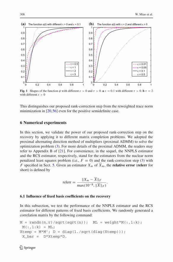
)1/τ if τ > 1. It should be good to choose an S-shaped function φ. But onealso needs to take account of the steepness of φ, which increases when τ increases.In particular for any ε satisfying 0 < ε < 1, φ approaches to the step function takingthe value 0 if 0 ≤ t < ε and the value 1 if ε < t ≤ 1 as τ → ∞. Since the rankof X is unknown and the singular values of Xm are unpredictable, choosing a large τ

could be risky. Therefore, one needs to choose τ with certain conservation, sacrificingcertain recovery quality in exchange for robustness strategically. Here, we provide arecommendation of the choices ε ≈ 0.05 (or within 0.01 ∼ 0.1) and τ = 2 (or within1 ∼ 3) for most cases, particularly when the initial estimator is generated from thenuclear norm penalized least squares problem. These choices have performed verystably for plenty of problems, as validated in Sect. 6.

We also remark that for the positive semidefinite case, the rank-correction functiondefined by (24), (25) and (26) is related to the reweighted trace norm for the matrixrank minimization proposed by Fazel et al. [20,56]. The reweighted trace norm in[20,56] for the positive semidefinite case is 〈(Xk + ε In)−1, X〉, which arises fromthe derivative of the surrogate function log det(X + ε In) of the rank at an iterate Xk ,where ε is a small positive constant. Meanwhile, in our proposed rank-correction step,if we choose τ = 1, then In − 1

1+εF(Xm) = ε′(Xm + ε′ In)−1 with ε′ = ε‖Xm‖.

Superficially, similarity occurs; however, it is notable that ε′ depends on Xm , which isdifferent from the constant ε in [20,56]. More broadly speaking, the rank-correctionfunction F defined by (24), (25) and (26) is not a gradient of any real-valued function.

123

308 W. Miao et al.

0 0.2 0.4 0.6 0.8 10

0.1

0.2

0.3

0.4

0.5

0.6

0.7

0.8

0.9

1The function φ(t) with different τ > 0 and ε = 0.1

τ = 0.5τ = 1τ = 2τ = 5

0 0.2 0.4 0.6 0.8 10

0.1

0.2

0.3

0.4

0.5

0.6

0.7

0.8

0.9

1The function φ(t) with τ = 2 and different ε > 0

ε = 0.01ε = 0.05ε = 0.1ε = 0.5

(a) (b)

Fig. 1 Shapes of the function φ with different ε > 0 and τ > 0. a ε = 0.1 with different τ > 0. b τ = 2with different ε > 0

This distinguishes our proposed rank-correction step from the reweighted trace normminimization in [20,56] even for the positive semidefinite case.

6 Numerical experiments

In this section, we validate the power of our proposed rank-correction step on therecovery by applying it to different matrix completion problems. We adopted theproximal alternating direction method of multipliers (proximal ADMM) to solve theoptimization problem (3). For more details of the proximal ADMM, the readers mayrefer to Appendix B of [21]. For convenience, in the sequel, the NNPLS estimatorand the RCS estimator, respectively, stand for the estimators from the nuclear normpenalized least squares problem (i.e., F ≡ 0) and the rank-correction step (3) withF specified in Sect. 5. Given an estimator Xm of Xm , the relative error (relerr forshort) is defined by

relerr = ‖Xm − X‖Fmax(10−8, ‖X‖F )

.

6.1 Influence of fixed basis coefficients on the recovery

In this subsection, we test the performance of the NNPLS estimator and the RCSestimator for different patterns of fixed basis coefficients. We randomly generated acorrelation matrix by the following command:

M = randn(n,r)/sqrt(sqrt(n)); ML = weight*M(:,1:k);M(:,1:k) = ML;

Xtemp = M*M’; D = diag(1./sqrt(diag(Xtemp)));X_bar = D*Xtemp*D.

123


We took the true matrix X = X_bar with dimension n = 500, rank r = 5, weight= 5 and k = 1. Here, the parameter weight is used to control the relative mag-nitude difference between the first k largest eigenvalues and the left r − k nonzeroeigenvalues. We randomly fixed partial diagonal and off-diagonal entries of X andthen uniformly sampled the rest entries with i.i.d. Gaussian noise. The noise level,defined by ‖νξ‖2/‖y‖2 in (2) hereafter, was set to be 10% and the upper bound of thenon-fixed diagonal entries was set to be 1. We further assumed that the rank of the truematrix was known so that for RCS estimator we chose the rank-correction function(23).

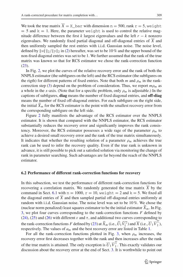
In Fig. 2, we plot the curves of the relative recovery error and the rank of both theNNPLS estimator (the subfigures on the left) and the RCS estimator (the subfigures onthe rigth) for different patterns of fixed entries. Note that both m and ρm in the rank-correction step (3) depend on the problem of consideration. Thus, we report mρm asa whole in the x-axis. (Note that for a specific problem, only ρm is adjustable.) In thecaptions of subfigures, diagmeans the number of fixed diagonal entries, and off-diagmeans the number of fixed off-diagonal entries. For each subfigure on the right side,the initial Xm for the RCS estimator is the point with the smallest recovery error fromthe corresponding subfigure on the left side.

Figure 2 fully manifests the advantage of the RCS estimator over the NNPLSestimator. It is shown that compared with the NNPLS estimator, the RCS estimatorsubstantially reduces the recovery error and significantly improves the rank consis-tency. Moreover, the RCS estimator possesses a wide rage of the parameter ρm toachieve a desired small recovery error and the rank of the true matrix simultaneously.It indicates that whether the resulting solution of a parameter ρm achieves the truerank can be used to infer the recovery quality. Even if the true rank is unknown inadvance, it is still possible to pick out a satisfied solution via monitoring the change ofrank in parameter searching. Such advantages are far beyond the reach of the NNPLSestimator.

6.2 Performance of different rank-correction functions for recovery

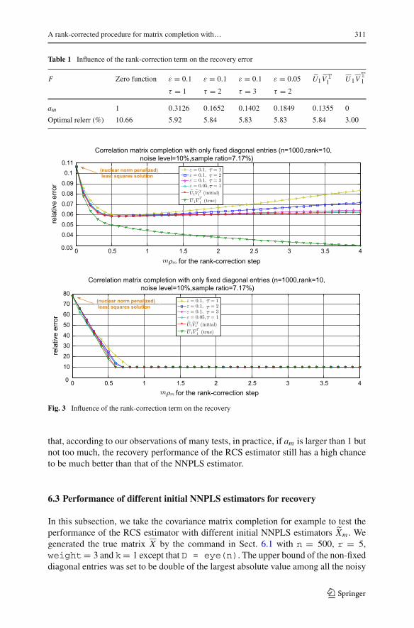
In this subsection, we test the performance of different rank-correction functions forrecovering a correlation matrix. We randomly generated the true matrix X by thecommand in Sect. 6.1 with n = 1000, r = 10, weight = 2 and k = 5. We fixed allthe diagonal entries of X and then sampled partial off-diagonal entries uniformly atrandom with i.i.d. Gaussian noise. The noise level was set to be 10%. We chose the(nuclear norm penalized) least squares estimator to be the initial estimator Xm . In Fig.3, we plot four curves corresponding to the rank-correction functions F defined by(24), (25) and (26) with different ε and τ , and additional two curves corresponding to

the rank-correction functions F defined by (23) at Xm (i.e., U1VT

1 ) and X (i.e.,U1VT

1 ),respectively. The values of am and the best recovery error are listed in Table 1.

For all the rank-correction functions plotted in Fig. 3, when ρm increases, therecovery error first decreases together with the rank and then increases after the rank

of the true matrix is attained. The only exception is U 1VT

1 . This exactly validates ourdiscussion about the recovery error at the end of Sect. 3. It is worthwhile to point out

123

310 W. Miao et al.

0 0.5 1 1.5 2 2.5 3 3.5 40.05

0.0750.1

0.1250.15

0.2

0.25

0.3

0.35

for the nuclear norm penalization

rela

tive

erro

r

0 0.5 1 1.5 2 2.5 3 3.5 40

5

10

20

30

40

rank

relative errorrank

m m

0 0.5 1 1.5 2 2.5 3 3.5 40.05

0.0750.1

0.1250.15

0.2

0.25

0.3

0.35

for the rank-correction step

rela

tive

erro

r

0 0.5 1 1.5 2 2.5 3 3.5 40

5

10

20

30

40

rank

relative errorrank

m m

0 0.5 1 1.5 2 2.5 3 3.5 40.05

0.0750.1

0.1250.15

0.2

0.25

0.3

0.35


rela

tive

erro

r

Number of fixed entries: diag = n/2, off-diag = 0

Number of fixed entries: diag = n/2, off-diag = 0

0 0.5 1 1.5 2 2.5 3 3.5 40

5

10

20

30

40

rank

relative errorrank

0 0.5 1 1.5 2 2.5 3 3.5 40.05

0.0750.1

0.1250.15

0.2

0.25

0.3

0.35


rela

tive

erro

r

0 0.5 1 1.5 2 2.5 3 3.5 40

5

10

20

30

40

rank

relative errorrank

0 0.5 1 1.5 2 2.5 3 3.5 40.05

0.0750.1

0.1250.15

0.2

0.25

0.3

0.35


rela

tive

erro

r

0 0.5 1 1.5 2 2.5 3 3.5 40

5

10

20

30

40

rank

relative errorrank

0 0.5 1 1.5 2 2.5 3 3.5 40.05

0.0750.1

0.1250.15

0.2

0.25

0.3

0.35


rela

tive

erro

r

Number of fixed entries: diag = n, off-diag = 0

Number of fixed entries: diag = n, off-diag = 0

0 0.5 1 1.5 2 2.5 3 3.5 40

5

10

20

30

40

rank

relative errorrank

0 0.5 1 1.5 2 2.5 3 3.5 40.05

0.0750.1

0.1250.15

0.2

0.25

0.3

0.35


rela

tive

erro

r

Number of fixed entries: diag = n, off-diag = n/2

Number of fixed entries: diag = 0, off-diag = 0

Number of fixed entries: diag = 0, off-diag = 0

Number of fixed entries: diag = n, off-diag = n/2

0 0.5 1 1.5 2 2.5 3 3.5 40

5

10

20

30

40

rank

relative errorrank

0 0.5 1 1.5 2 2.5 3 3.5 40.05

0.0750.1

0.1250.15

0.2

0.25

0.3

0.35


rela

tive

erro

r

0 0.5 1 1.5 2 2.5 3 3.5 40

5

10

20

30

40

rank

relative errorrank

(a) (b)

(d)(c)

(e) (f)

(h)(g)

ρ ρ

m mρm mρ

m mρ m mρ

m mρm mρ

Fig. 2 Influence of fixed basis coefficients on recovery (sample ratio = 6.4%). a Nuclear norm: diag = 0,off-diag = 0. b Rank-correction step: diag = 0, off-diag = 0. c Nuclear norm: diag = n/2, off-diag = 0. dRank-correction step: diag = n/2, off-diag = 0. e Nuclear norm: diag = n, off-diag = 0. f Rank-correctionstep: diag = n, off-diag = 0. g Nuclear norm: diag = n, off-diag = n/2. f Rank-correction step: diag = n,off-diag = n/2

123


Table 1 Influence of the rank-correction term on the recovery error

F Zero function ε = 0.1 ε = 0.1 ε = 0.1 ε = 0.05 U1VT1 U1V

T

1

τ = 1 τ = 2 τ = 3 τ = 2

am 1 0.3126 0.1652 0.1402 0.1849 0.1355 0

Optimal relerr (%) 10.66 5.92 5.84 5.83 5.83 5.84 3.00

0 0.5 1 1.5 2 2.5 3 3.5 40.03

0.040.05

0.060.07

0.080.09

0.10.11

Correlation matrix completion with only fixed diagonal entries (n=1000,rank=10, noise level=10%,sample ratio=7.17%)


rela

tive

erro

r

ε .1,ε .1,ε .1,ε .05,

= 0 = 1= 0 = 2= 0 = 3= 0 = 1

˜U1˜VT1 (initial)

U 1VT1 (true)

(nuclear norm penalized) least squares solution

m m

0 0.5 1 1.5 2 2.5 3 3.5 40

10

20

30

40

50

60

70

80

Correlation matrix completion with only fixed diagonal entries (n=1000,rank=10, noise level=10%,sample ratio=7.17%)


rela

tive

erro

r

ε .1,ε .1,ε .1,ε

= 0= 0= 0= 0.05,

= 1= 2= 3= 1

˜U1˜VT1 (initial)

U 1VT1 (true)

(nuclear norm penalized) least squares solution

ρ

m mρ

Fig. 3 Influence of the rank-correction term on the recovery

that, according to our observations of many tests, in practice, if am is larger than 1 butnot too much, the recovery performance of the RCS estimator still has a high chanceto be much better than that of the NNPLS estimator.

6.3 Performance of different initial NNPLS estimators for recovery

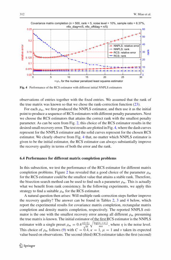
In this subsection, we take the covariance matrix completion for example to test theperformance of the RCS estimator with different initial NNPLS estimators Xm . Wegenerated the true matrix X by the command in Sect. 6.1 with n = 500, r = 5,weight= 3 and k= 1 except that D = eye(n). The upper bound of the non-fixeddiagonal entries was set to be double of the largest absolute value among all the noisy

123

312 W. Miao et al.

0.05

0.075

0.1

0.125

0.15

0.2

0.25

rela

tive

erro

r

for the nuclear penalized least squares estimator

Covariance matrix completion (n = 500, rank = 5, noise level = 10%, sample ratio = 6.37%, nfix_diag=n/5, nfix_offdiag = n/5)

0 5 10 15 20 25 300510

20

30

40

50

60

rank

NNPLS: relative errorNNPLS: rankRCS: relative errorRCS: rank

m mρ

Fig. 4 Performance of the RCS estimator with different initial NNPLS estimators

observations of entries together with the fixed entries. We assumed that the rank ofthe true matrix was known so that we chose the rank-correction function (23).

For each ρm , we first produced the NNPLS estimator, and then use it as the initialpoint to produce a sequence of RCS estimators with different penalty parameters. Nextwe choose the RCS estimators that attains the correct rank with the smallest penaltyparameter. As can be seen from Fig. 2, this choice of the RCS estimator results in thedesired small recovery error. The test results are plotted in Fig. 4, where the dash curvesrepresent for the NNPLS estimator and the solid curves represent for the chosen RCSestimator. We clearly observe from Fig. 4 that, no matter which NNPLS estimator isgiven to be the initial estimator, the RCS estimator can always substantially improvethe recovery quality in terms of both the error and the rank.

6.4 Performance for different matrix completion problems

In this subsection, we test the performance of the RCS estimator for different matrixcompletion problems. Figure 2 has revealed that a good choice of the parameter ρmfor the RCS estimator could be the smallest value that attains a stable rank. Therefore,the bisection search method can be used to find such a parameter ρm . This is actuallywhat we benefit from rank consistency. In the following experiments, we apply thisstrategy to find a suitable ρm for the RCS estimator.

A natural question then arises: Will multiple rank-correction steps further improvethe recovery quality? The answer can be found in Tables 2, 3 and 4 below, whichreport the experimental results for covariance matrix completion, rectangular matrixcompletion and density matrix completion, respectively. The reported NNPLS esti-mator is the one with the smallest recovery error among all different ρm presumingthe true matrix is known. The initial estimator of the first RCS estimator is the NNPLS

estimator with a single preset ρm = 0.4 η‖y‖2√m

√log(n1+n2)

mn , where η is the noise level.This choice of ρm follows (9) with C = 0.4, κ = 1, μ = 1 and ν taken its expectedvalue based on observations. The second (third) RCS estimator takes the first (second)

123


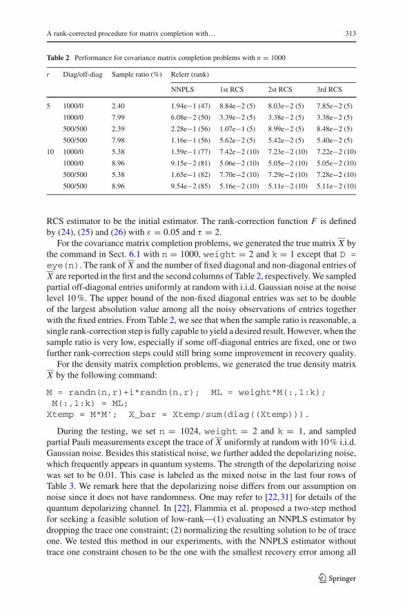
Table 2 Performance for covariance matrix completion problems with n = 1000

r Diag/off-diag Sample ratio (%) Relerr (rank)

NNPLS 1st RCS 2st RCS 3rd RCS

5 1000/0 2.40 1.94e−1 (47) 8.84e−2 (5) 8.03e−2 (5) 7.85e−2 (5)

1000/0 7.99 6.08e−2 (50) 3.39e−2 (5) 3.38e−2 (5) 3.38e−2 (5)

500/500 2.39 2.28e−1 (56) 1.07e−1 (5) 8.99e−2 (5) 8.48e−2 (5)

500/500 7.98 1.16e−1 (56) 5.62e−2 (5) 5.42e−2 (5) 5.40e−2 (5)

10 1000/0 5.38 1.59e−1 (77) 7.42e−2 (10) 7.23e−2 (10) 7.22e−2 (10)

1000/0 8.96 9.15e−2 (81) 5.06e−2 (10) 5.05e−2 (10) 5.05e−2 (10)

500/500 5.38 1.65e−1 (82) 7.70e−2 (10) 7.29e−2 (10) 7.28e−2 (10)

500/500 8.96 9.54e−2 (85) 5.16e−2 (10) 5.11e−2 (10) 5.11e−2 (10)

RCS estimator to be the initial estimator. The rank-correction function F is definedby (24), (25) and (26) with ε = 0.05 and τ = 2.

For the covariance matrix completion problems, we generated the true matrix X bythe command in Sect. 6.1 with n = 1000, weight = 2 and k = 1 except that D =eye(n). The rank of X and the number of fixed diagonal and non-diagonal entries ofX are reported in the first and the second columns of Table 2, respectively.We sampledpartial off-diagonal entries uniformly at random with i.i.d. Gaussian noise at the noiselevel 10%. The upper bound of the non-fixed diagonal entries was set to be doubleof the largest absolution value among all the noisy observations of entries togetherwith the fixed entries. From Table 2, we see that when the sample ratio is reasonable, asingle rank-correction step is fully capable to yield a desired result. However, when thesample ratio is very low, especially if some off-diagonal entries are fixed, one or twofurther rank-correction steps could still bring some improvement in recovery quality.

For the density matrix completion problems, we generated the true density matrixX by the following command:

M = randn(n,r)+i*randn(n,r); ML = weight*M(:,1:k);M(:,1:k) = ML;

Xtemp = M*M’; X_bar = Xtemp/sum(diag((Xtemp))).

During the testing, we set n = 1024, weight = 2 and k = 1, and sampledpartial Pauli measurements except the trace of X uniformly at random with 10% i.i.d.Gaussian noise. Besides this statistical noise, we further added the depolarizing noise,which frequently appears in quantum systems. The strength of the depolarizing noisewas set to be 0.01. This case is labeled as the mixed noise in the last four rows ofTable 3. We remark here that the depolarizing noise differs from our assumption onnoise since it does not have randomness. One may refer to [22,31] for details of thequantum depolarizing channel. In [22], Flammia et al. proposed a two-step methodfor seeking a feasible solution of low-rank—(1) evaluating an NNPLS estimator bydropping the trace one constraint; (2) normalizing the resulting solution to be of traceone. We tested this method in our experiments, with the NNPLS estimator withouttrace one constraint chosen to be the one with the smallest recovery error among all

123

314 W. Miao et al.

Table3

Performance

fordensity

matrixcompletionproblemswith

n=

1024

Noise

rNoise

level(%)

Sampleratio

(%)

NNPL

S1NNPL

S2RCS

Fidelity

Relerr

Rank

Fidelity

Relerr

Rank

Fidelity

Relerr

Rank

Statistical

310.0

1.5

0.716

2.49e−

13

0.96

22.34

e−1

30.99

28.47

e−2

3

10.0

4.0

0.91

58.14

e−2

30.99

76.88

e−2

30.99

84.13

e−2

3

510

.02.5

0.69

62.56

e−1

50.95

92.71

e−1

50.99

28.28

e−2

5

10.0

5.0

0.88

61.04

e−1

50.99

49.61

e−2

50.99

74.81

e−2

5

Mixed

312

.51.5

0.65

72.95

e−1

30.95

92.41

e−1

30.99

09.89

e−2

3

12.4

4.0

0.84

21.42

e−1

30.99

67.48

e−2

30.99

76.20

e−2

3

512

.42.5

0.63

13.05

e−1

50.95

42.87

e−1

50.99

09.81

e−2

5

12.5

5.0

0.81

41.62

e−1

50.99

41.03

e−1

50.99

66.94

e−2

5

123


Table4

Performance

forrectangu

larmatrixcompletionprob

lems

Setting

Sample

Fixed

Sampleratio

(%)

Relerr(rank)

NNPL

S1stR

CS

2stR

CS

3rdRCS

dim

=10

00×

1000

,rank

=10

Uniform

05.97

1.98

e−1(119

)7.69

e−2(10)

7.31

e−2(10)

7.30

e−2(10)

011

.98.34

e−2(114

)4.49

e−2(10)

4.48

e−2(10)

4.48

e−2(10)

1000

5.98

1.93

e−1(120

)7.45

e−2(10)

7.01

e−2(10)

7.00

e−2(10)

1000

12.0

8.20

e−2(108

)4.35

e−2(10)

4.34

e−2(10)

4.34

e−2(10)

Non

-uniform

05.97

3.20

e−1(144

)1.22

e−1(10)

9.31

e−2(10)

8.77

e−2(10)

011

.91.27

e−1(171

)5.32

e−2(10)

5.12

e−2(10)

5.11

e−2(10)

1000

5.98

3.07

e−1(146

)1.16

e−1(10)

8.78

e−2(10)

8.30

e−2(10)

1000

12.0

1.24

e−1(173

)5.14

e−2(10)

4.93

e−2(10)

4.92

e−2(10)

dim

=50

0×

1500

,rank

=5

Uniform

03.99

2.31

e−1(73)

9.15

e−2(5)

8.10

e−2(5)

7.95

e−2(5)

07.98

9.01

e−2(78)

4.60

e−2(5)

4.58

e−2(5)

4.58

e−2(5)

1000

4.00

2.15

e−1(74)

8.77

e−2(5)

7.58

e−2(5)

7.36

e−2(5)

1000

7.99

8.72

e−2(69)

4.34

e−2(5)

4.31

e−2(5)

4.31

e−2(5)

Non

-uniform

03.99

3.37

e−1(91)

1.53

e−1(5)

1.18

e−1(5)

1.07

e−1(5)

07.98

1.37

e−1(128

)5.62

e−2(5)

5.33

e−2(5)

5.31

e−2(5)

1000

4.00

3.11

e−1(93)

1.39

e−1(6)

1.06

e−1(5)

9.55

e−2(5)

1000

7.99

1.29

e−1(104

)5.21

e−2(5)

4.91

e−2(5)

4.89

e−2(5)

123

316 W. Miao et al.

that attain the true rank, presuming that the true matrix is known. The two-step resultsare reported as NNPLS1 and NNPLS2, respectively, in Table 3. Besides the relativerecovery error (relerr), we also report the (squared) fidelity, which is a measure of

the closeness of two quantum states defined by∥∥X1/2

m X1/2∥∥2∗. From Table 3, we can

see that the RCS estimator is superior to the NNPLS2 estimator in terms of both thefidelity and the relative error.

For the rectangular matrix completion problems, we generated the true matrix Xby the following command:

ML = randn(nr,r); MR = randn(nc,r);MW = weight*ML (:,1:k);

ML(:,1:k) = MW; X_bar = ML*MR’.

Wesetweight= 2,k= 1 and took X =X_barwith different dimensions and ranks.Both the uniform sampling scheme and the non-uniform sampling scheme were testedfor comparison. For the non-uniform sampling scheme, the probability to sample thefirst 1/4 rows and the first 1/4 columns were 3 times as much as that of other rows andcolumns respectively. In other words, the density of sampled entries in the top-left partwas 3 times as much as that in the bottom-left part and the top-right part respectivelyand 9 times as much as that in the bottom-right part. We added 10% i.i.d. Gaussiannoise to the sampled entries. We also fixed partial entries of X uniformly from the restun-sampled entries. The upper bound of the non-fixed entries was set to be double ofthe largest absolution value among all the noisy observations of entries together withthe fixed entries. What we observe from Table 4 for the rectangular matrix completionis similar to that for the covariance matric completion. Moreover, we can see thatthe non-uniform sampling scheme greatly weakens the recoverability of the NNPLSestimator in terms of both the recovery error and the rank, especially when the sampleratio is low. Meanwhile, the advantage of the RCS estimators in such cases becomesmore remarkable.

7 Conclusions

In this paper, we proposed a rank-corrected procedure for low-rank matrix completionproblems with fixed basis coefficients. This approach can substantially overcome thelimitation of the nuclear norm technique for recovering a low-rank matrix. We con-firmed the improvement of the rank-correction step in both the reduction of recoveryerror and the achievement of rank consistency (in the sense of Bach [3]). Due to thepresence of fixed basis coefficients, constraint nondegeneracy plays an important rolein our analysis. Extensive numerical experiments show that our approach can signifi-cantly improve the recovery performance compared with the nuclear norm penalizedleast square estimator. As a byproduct, our results also provide a theoretical foundationfor the majorized penalty method of Gao and Sun [27] and Gao [26] for structuredlow-rank matrix optimization problems.

Our proposed rank-correction step also allows additional constraints according toother possible prior information. In order to better fit the under-sampling setting ofmatrix completion, in the future work, it would be of great interest to extend the

123


asymptotic rank consistency results to the case where the matrix size is allowed togrow. It would also be interesting to extend this approach to deal with other low-rankmatrix problems.

Acknowledgments The authors would like to thank Professor Wotao Yin for his valuable comments onpossibly choosing the optimal penalty parameter for recovery error bounds andDr. Kaifeng Jiang for helpfuldiscussions on efficiently solving the density matrix completion problem.

Appendix 1: Spectral operator

The concept of spectral operator is associatedwith a symmetric vector-valued function.A function f : Rn → R

n is said to be symmetric if

f (x) = QT f (Qx) ∀ signed permutation matrix Q and x ∈ Rn,

where a signed permutation matrix is a real matrix that contains exactly one nonzeroentry 1 or −1 in each row and column and 0 elsewhere. From this definition, we seethat

fi (x) = 0 if xi = 0.

The spectral operator F : Vn1×n2 → Vn1×n2 associated with the function f is defined

by

F(X) := UDiag(f (σ (X))

)VT, (27)

where (U, V ) ∈ On1,n2(X) and X ∈ V

n1×n2 . From [10, Theorems 3.1 & 3.6], thesymmetry of f guarantees the well-definiteness of the spectral operator F , and the(continuous) differentiability of f implies the (continuous) differentiability of F .When V

n1×n2 = Sn , we have that

F(X) = PDiag(f (|λ(X)|))(PDiag(s(X))

)T,

where P ∈ On(X) and s(X) ∈ R

n with the i-th component si (X) = −1 if λi (X) < 0and si (X) = 1 otherwise. In particular for the positive semidefinite case, both U andV in (27) reduce to P . For more details on spectral operators, the readers may referto the PhD thesis [10].

Appendix 2: Constraint nondegeneracy

Consider the following constrained optimization problem

minX∈Vn1×n2

{�(X) + �(X) : A(X) − b ∈ K

}, (28)

123

318 W. Miao et al.

where � : Vn1×n2 → R is a continuously differentiable function, � : Vn1×n2 → R

is a convex function, A : Vn1×n2 → Rl is a linear operator and K ⊆ R

l is a closedconvex set. Let X be a given feasible point of (28) and z := A(X) − b. When � isdifferentiable at X , we say that the constraint nondegeneracy holds at X if

AVn1×n2 + lin

(TK (z)

) = Rl , (29)

where TK (z) denotes the tangent cone of K at z and lin(TK (z)) denotes the largestlinearity space contained in TK (z), i.e., lin(TK (z)) = TK (z) ∩ (−TK (z)). When thefunction � is nondifferentiable, we can rewrite the optimization problem (28) equiv-alently as

minX∈Vn1×n2 ,t∈R

{�(X) + t : A(X, t) ∈ K × epi�

},

where epi� := {(X, t) ∈ V

n1×n2 × R | �(X) ≤ t}denotes the epigraph of � and

A : Vn1×n2 × R → Rl × V

n1×n2 × R is a linear operator defined by

A(X, t) :=⎛

⎝A(X) − b

Xt

⎞

⎠ , (X, t) ∈ Vn1×n2 × R.

From (29) and [67, Theorem 6.41], the constraint nondegeneracy holds at (X , t) witht = �(X) if

A(Vn1×n2

R

)+(

lin(TK (z)

)

lin(Tepi�(X , t)

))

=⎛

⎝Rl

Vn1×n2

R

⎞

⎠ .

By the definition of A, it is not difficult to verify that this condition is equivalent to

[A 0](lin(Tepi�(X , t)))+ lin

(TK (z)

) = Rl . (30)

One can see that the problem (3) with C = Vn1×n2 can be cast into (28) with

� = ‖ · ‖∗,A = [Rα Rβ ], K = {0}|α| × [−b, b]|β|, and meanwhile the problem (3)with C = S

n+ can be cast into (28) with � = δSn+ ,A = Rα , K = {0}. In the previous

case, the condition (30) reduces to (15) according to the expression of Tepi�(X , t)with t = ‖X‖∗ (e.g., see [34]). In the latter case, the condition (30) reduces to (16)according to Arnold’s characterization of the tangent cone TSn+(X) = {

H ∈ Sn |

PT

2 HP2 ∈ Sn−r+}in [2].

123


Appendix 3: Proofs of Theorems

Proof of Theorem 1

Let �m := Xm − X . Using the optimality of Xm to the problem (3), we obtain that

1

2m‖R�(�m)‖22 ≤

⟨ νmR∗

�(ξ),�m

⟩− ρm

(‖Xm‖∗ − ‖X‖∗ − 〈F(Xm),�m〉). (31)

Then, we introduce an orthogonal decomposition Vn1×n2 = T ⊕ T⊥ with

{T := {X ∈ V

n1×n2 | X = X1 + X2 with col(X1) ⊆ col(X) and row(X2) ⊆ row(X)},

T⊥ := {X ∈ Vn1×n2 | row(X) ⊥ row(X) and col(X) ⊥ col(X)

},

where row(X) and col(X) denote the row space and column space of X , respectively.Let PT and PT⊥ be orthogonal projections onto T and T⊥, respectively, given by

PT (X) = U 1UT

1 X + XV 1VT

1 −U1UT

1 XV 1VT

1 and PT⊥(X) = U 2UT

2 XV 2VT

2(32)

for any X ∈ Vn1×n2 and (U , V ) ∈ O

n1,n2(X). Then, it follows from the choice of ρmthat⟨ νmR∗

�(ξ),�m

⟩≤∥∥∥ν

mR∗

�(ξ)

∥∥∥‖�m‖∗ ≤ ρm

κ

(‖PT (�m)‖∗ + ‖PT⊥(�m)‖∗). (33)

Moreover, from the directional derivative of the nuclear norm at X , (see [75, Theo-rem 1]), we have

‖Xm‖∗ − ‖X‖∗ − 〈F(Xm),�m〉 ≥ 〈U 1VT

1 ,�m〉 + ‖UT

2�mV 2‖∗ − 〈F(Xm),�m〉≥ ‖PT⊥(�m)‖∗ − ‖U 1V

T

1 − F(Xm)‖F‖�m‖F= ‖PT⊥(�m)‖∗ − am

√r‖�m‖F . (34)

Then, by substituting (33) and (34) into (31), we have

1

2m‖R�(�m)‖22 ≤ ρm

(am

√r‖�m‖F + 1

κ‖PT (�m)‖∗ − κ − 1

κ‖PT⊥(�m)‖∗

).

(35)Note that rank(PT (�m)) ≤ 2r . Hence, ‖PT (�m)‖∗ ≤ √

2r‖PT (�m)‖F ≤√2r‖�m‖F and then the desired result (7) follows.

Proof of Theorem 2

We first show that the sampling operator R� satisfies some RIP-like property formatrices specified in a certain set with high probability. Similar results can also befound in [40,44,49,58].

123

320 W. Miao et al.

For this purpose, define

ϑm := E

∥∥∥1

mR∗

�(ε)

∥∥∥ with ε = (ε1, . . . , εm)T, (36)

where {ε1, . . . , εm} is an i.i.d. Rademacher sequence, i.e., an i.i.d. sequence ofBernoulli random variables taking the values 1 and −1 with probability 1/2.

Lemma 11 Given any s > 0 and t > 0, define

K (s, t) :={� ∈ Vn1×n2

∣∣Rα(�) = 0, ‖Rβ(�)‖∞ = 1, ‖�‖∗ ≤ s‖�‖F ,〈Qβ(�),�〉 ≥ t

}.

Then, for any given γ > 1, τ1 ∈ (0, 1) and τ2 ∈ (0, τ1/γ ), with probability at least

1 − exp(−(τ1−γ τ2)2mt2/2)

1−exp(−(γ 2−1)(τ1−γ τ2)2mt2/2),

1

m‖R�(�)‖22 ≥ (1 − τ1)〈Qβ(�),�〉 − 16

τ2s2μ1d2ϑ

2m ∀� ∈ K (s, t). (37)

Proof The proof is similar to that of [40, Lemma 12]. For any s, t > 0, γ > 1,τ1 ∈ (0, 1) and τ2 ∈ (0, τ1/γ ), we need to show that the event

E ={∃�∈K (s, t) such that

∣∣∣1

m‖R�(�)‖22 − 〈Qβ(�),�〉

∣∣∣

≥ τ1〈Qβ(�),�〉 + 16

τ2s2μ1d2ϑ

2m

}

occurs with probability less than exp(−(τ1−γ τ2)2mt2/2)

1−exp(−(γ 2−1)(τ1−γ τ2)2mt2/2). We decompose K (s, t)

as

K (s, t) =∞⋃

k=1

{� ∈ K (s, t)

∣∣ γ k−1t ≤ 〈Qβ(�),�〉 ≤ γ k t

}.

For any a ≥ t , we further define K (s, t, a) := {� ∈ K (s, t) | 〈Qβ(�),�〉 ≤ a}.Then we get E ⊆⋃∞

k=1 Ek with

Ek ={∃�∈K (s, t, γ k t) such that

∣∣∣1

m‖R�(�)‖22 − 〈Qβ(�),�〉

∣∣∣

≥ γ k−1τ1t + 16

τ2s2μ1d2ϑ

2m

}.

Now we need to estimate the probability of each event Ek . Define

Za := sup�∈K (s,t,a)

∣∣∣1

m‖R�(�)‖22 − 〈Qβ(�),�〉

∣∣∣.

123


Notice that for any � ∈ Vn1×n2 ,

1

m‖R�(�)‖22 = 1

m

m∑

i=1

〈�ωi ,�〉2 a.s.→ E(〈�ωi ,�〉2) = 〈Qβ(�),�〉.

Since ‖Rβ(�)‖∞ ≤ 1 for all� ∈ K (s, t), fromMassart’s Hoeffding type concentra-tion inequality [51, Theorem 1.4] for suprema of empirical processes, we have

Pr(Za ≥ E(Za) + ε

) ≤ exp

(−mε2

2

)∀ ε > 0. (38)

Next, we use the standard Rademacher symmetrization in the theory of empiricalprocesses to further derive an upper bound ofE(Za). Let {ε1, . . . , εm} be aRademachersequence. Then, we have

E(Za) = E

(sup

�∈K (s,t,a)

∣∣∣1

m

m∑

i=1

〈�ωi ,�〉2 − E(〈�ωi ,�〉2)

∣∣∣)

≤ 2E

(sup

�∈K (s,t,a)

∣∣∣1

m

m∑

i=1

εi 〈�ωi ,�〉2∣∣∣)

≤ 8E

(sup

�∈K (s,t,a)

∣∣∣1

m

m∑

i=1

εi 〈�ωi ,�〉∣∣∣)

= 8E

(sup

�∈K (s,t,a)

∣∣∣1

m

m∑

i=1

〈R∗�(ε),�〉

∣∣∣)

≤ 8E∥∥∥1

mR∗

�(ε)

∥∥∥(

sup�∈K (s,t,a)

‖�‖∗),

(39)

where the first inequality follows from the symmetrization theorem (e.g., see [73,Lemma 2.3.1] and [6, Theorem 14.3]) and the second inequality follows from thecontraction theorem (e.g., see [46, Theorem 4.12] and [6, Theorem 14.4]). Moreover,from (8), we have

〈Qβ(�),�〉 ≥ (μ1d2)−1‖�‖2F ∀� ∈ {�∈V

n1×n2 | Rα(�) = 0}. (40)

This leads to

‖�‖∗ ≤ s‖�‖F ≤ s√μ1d2〈Qβ(�),�〉 ≤ s

√μ1d2a ∀� ∈ K (s, t, a). (41)

Combining (39) and (41) with the definition of ϑm in (36), we obtain that

E(Za) +(τ1γ

− τ2

)a ≤ 8ϑms

√μ1d2a +

(τ1γ

− τ2

)a ≤ 16

τ2s2μ1d2ϑ

2m + τ1

γa,

where the second inequality follows from the simple fact x1x2 ≤ (x21 + x22 )/2 for anyx1, x2 ≥ 0. Then, it follows from (38) that

123

322 W. Miao et al.

Pr

(Za ≥ τ1

γa + 16

τ2s2μ1d2ϑ

2m

)≤ Pr

(Za ≥ E(Za) +

(τ1γ

−τ2

)a

)

≤ exp

(−(τ1γ

−τ2

)2 ma2

2

).

This implies that Pr(Ek) ≤ exp(− 1

2 γ 2(k−1)(τ1 − γ τ2)2mt2

). Then, since γ > 1, by

using γ k ≥ 1 + k(γ − 1) for any k ≥ 1, we have

Pr(E) ≤∞∑

k=1

Pr(Ek) ≤∞∑

k=1

exp(− 1

2γ 2(k−1)(τ1 − γ τ2)

2mt2)

≤ exp(− 1

2(τ1 − γ τ2)

2mt2) ∞∑

k=1

exp(− 1

2(k − 1)(γ 2 − 1)(τ1 − γ τ2)

2mt2)

≤ exp(−(τ1 − γ τ2)2mt2/2)

1 − exp(−(γ 2 − 1)(τ1 − γ τ2)2mt2/2).

Thus, we complete the proof of Lemma 11.

Now we proceed with the proof of Theorem 2. Let�m := Xm − X . Notice that theequality (35) implies that

‖PT⊥(�m)‖∗ ≤ 1

κ − 1‖PT (�m)‖∗ + κ

κ − 1am

√r‖�m‖F .

This, together with ‖PT (�m)‖∗ ≤ √2r‖�m‖F , leads to

‖�m‖∗ ≤ ‖PT (�m)‖∗ + ‖PT⊥(�m)‖∗ ≤ κ

κ − 1

(√2 + am

)√r‖�m‖F . (42)

Let bm := ‖Rβ(�m)‖∞ ≤ 2b. For any fixed c > 0, γ > 1, τ1 ∈ (0, 1) and

τ2 ∈ (0, τ2/γ ), define tm :=√

2c log(n1+n2)(τ1−γ τ2)2m

so that direct calculation yields

exp(−(τ1 − γ τ2)2mt2m/2)

1 − exp(−(γ 2 − 1)(τ1 − γ τ2)2mt2m/2)= (n1 + n2)−c

1 − (n1 + n2)−(γ 2−1)c≤ (n1 + n2)−c

1 − 2−(γ 2−1)c.

Then we separate the discussion into two cases:

Case 1: 〈Qβ(�m),�m〉 ≤ b2mtm . It follows from (40) that ‖�m‖2F/d2 ≤ 4b2μ1tm .

Case 2: 〈Qβ(�m),�m〉 > b2mtm . It follows from (42) that �m/bm ∈ K (sm, tm) withsm := κ

κ−1

(√2+am

)√r . Then for any given τ3 satisfying 0 < τ3 < 1, we obtain that

with probability at least 1 − (n1+n2)−c

1−2−(γ 2−1)c,

123


‖�m‖2Fd2

≤ μ1〈Qβ(�m),�m〉 ≤ μ1

1 − τ1

(1

m‖R�(�m)‖22 + 16

τ2s2mμ1d2ϑ

2mb

2m

)

≤ 2

1 − τ1

(√2

κ+ am

)μ1ρm

√r‖�m‖F + 16

(1 − τ1)τ2s2mμ

21d2ϑ

2mb

2m

≤ τ3‖�m‖2F

d2+ 2

(1 − τ1)2τ3

(√2

κ+ am

)2

μ21ρ

2mrd2 + 16

(1 − τ1)τ2s2mμ

21d2ϑ

2mb

2m,

where the first inequality follows from (40), the second inequality follows fromLemma 11 and the third inequality follows from Theorem 1. Plugging in sm furtherleads to

‖�m‖2Fd2

≤ μ21d2r

1 − τ3

(2

(1−τ1)2τ3

(√2

κ+ am

)2

ρ2m + 64

(1 − τ1)τ2

(κ

κ−1

)2(√2 + am

)2ϑ2mb

2

)

.

Combing the above two cases together, with γ , τ1, τ2 and τ3 chosen to be absoluteconstants, we arrive at an intermediate result that there exist some positive absoluteconstants c′

0, c′1, c

′2 and C ′

0 such that for any κ > 1, if ρm is chosen as in Theorem 1,then with probability at least 1 − c′

1(n1 + n2)−c′2 ,

‖Xm − X‖2Fd2

≤ C ′0 max

{μ21d2r

(

c′02(√

2

κ+ am

)2ρ2m +

(κ

κ − 1

)2(√2 + am

)2ϑ2mb

2

)

,

b2μ1

√log(n1 + n2)

m

}. (43)

To further derive explicit estimations of ρm and ϑm , we introduce the noncom-mutative Bernstein inequality taken from [42, Corollary 2.1], which provides aprobability control of the deviation of the sum of random matrices from its meanin the operator norm. The noncommutative Bernstein inequality introduced hereis a recently-extended version, with the random matrices being controlled by theOrlicz norms (see [42–44]) rather than the operator norm (see, e.g., [30,63,72]).The Orlicz norms are used to characterize the tail behavior of random variables.Given any s ≥ 1, the ψs Orlicz norm of a random variable z is defined by‖z‖ψs := inf{t > 0

∣∣E exp(|z|s/t s) ≤ 2}.

Lemma 12 (Koltchinskii [42]) Let Z1, . . . , Zm ∈ Vn1×n2 be independent random

matrices with mean zero. Suppose thatmax{∥∥‖Zi‖

∥∥ψs

, 2E12 (‖Zi‖2)

}< �s for some

constant �s . Define

σZ := max

{∥∥∥∥1

m

m∑

i=1

E(Zi ZT

i )

∥∥∥∥

1/2

,

∥∥∥∥1

m

m∑

i=1

E(ZT

i Zi )

∥∥∥∥

1/2}

.

123

324 W. Miao et al.

Then, there exists a constant C such that for all t > 0, with probability at least1− exp(−t),

∥∥∥∥1

m

m∑

i=1

Zi

∥∥∥∥ ≤ C max

{

σZ

√t + log(n1 + n2)

m,�s

(log

�s

σZ

)1/s t + log(n1+ n2)

m

}

.

With the help of Lemma 12, we obtain the following result, which is an extensionof [44, Lemma 2] and [40, Lemmas 5 and 6] from the standard basis to an arbitraryorthonormal basis. A similar result can also be found in [58, Lemma 6].

Lemma 13 Under Assumption 2, there exists a positive constant C ′ (only dependingon the ψ1 Orlicz norm of ξk) such that for all t > 0, with probability at least 1 −exp(−t),

∥∥∥∥1

mR∗

�(ξ)

∥∥∥∥ ≤ C ′ max

{√μ2(t+ log(n1+ n2))√

d2m,log(d2)(t+ log(n1+ n2))

2m

}

.

(44)In particular, when m ≥ √

d2 log3(n1 + n2)/μ2, we also have

E

∥∥∥∥1

mR∗

�(ξ)

∥∥∥∥ ≤ C ′

√2eμ2 log(n1 + n2)√

d2m, (45)

where e is the exponential constant.

Proof Recall that 1mR∗

�(ξ) = 1m

∑mi=1 ξi�ωi . Let Zi := ξi�ωi . Since E(ξi ) = 0, the

independence of ξi and �ωi implies that E(Zi ) = 0. Since ‖�ωi ‖F = 1, we havethat ‖Zi‖ ≤ ‖Zi‖F = |ξi |‖�ωi ‖F = |ξi |. It follows that

∥∥‖Zi‖∥∥ψ1

≤ ‖ξi‖ψ1 andthus finite. (It is known that a random variable is sub-exponential if and only its ψ1

Orlicz norm is finite [73]). Meanwhile, E12 (‖Zi‖2) ≤ E

12 (‖Zi‖2F ) = E

12 (ξ2i ) = 1.

Then direct calculation yields

E(Zi Z

T

i

) = E(ξ2i �ωi�

Tωi

) = E(�ωi�

Tωi

) =∑

k∈βpk�k�

T

k .

The calculation for E(ZT

i Zi)is similar. We obtain from (8) that 1/

√d2 ≤ σ 2

Z ≤μ2/

√d2. Then, applying this to Lemma 12 yields (44). The remaining proof of (45)

follows the same as the proof of Lemma 6 in [40]. For simplicity, we omit it.

A good estimation ofρm can be achieved by choosing t = c′2 log(n1+n2) in Lemma

13 for an optimal order bound, where c′2 is the same as that in (43). With this choice,

when m ≥ 4(1+ c′2)

√d2 log2(d2) log(n1 + n2)/μ2, the first term in the maximum of

(44) dominates the second one. Thus, with probability at least 1 − (n1 + n2)−c′2 , one

can choose

ρm = κν · C ′√

(1 + c′2)μ2 log(n1 + n2)√

d2m.

123


Moreover, since Bernoulli random variables are sub-exponential, Lemma 13 also pro-vides an upper bound of ϑm in (45). It is worthwhile to note that after plugging theabove estimations of ρm and ϑm , the second term in the maximum of (43) is negli-gible compared with the first term. Therefore, the second term is further dropped forsimplicity and thus we complete the proof.

Proof of Theorem 3

For notational simplicity, we drop the subscript of Xm in this proof. With (U , V ) ∈O

n1,n2(X), one immediately obtains from the definition of am in (6) that

am ≤ 1√r

(‖F(X) − U1VT

1 ‖F + ‖U1VT

1 −U1VT

1 ‖F) ≤ εF (X) + 1√

r‖U1V

T

1 −U1VT

1 ‖F .(46)

The left proof is to find an upper bound of ‖U1VT

1 − U1VT

1 ‖F . Let δ := ‖X − X‖Fand Nδ(X) := {X ∈ V

n1×n2 | ‖X − X‖F ≤ δ}.Let F : V

n1×n2 → Vn1×n2 be a spectral operator associated with a symmetric

function f : Rn → Rn given by fi (x) = φ(xi ), i = 1, . . . , n, where φ : R → R is

an odd scalar function with φ(t) = −φ(−t) for t < 0, and φ(t) for t ≥ 0 is definedas

φ(t) =

⎧⎪⎪⎨

⎪⎪⎩

1 if t ≥ 2σr (X)/3 − δ/3,t−(σr (X)/3+δ/3)σr (X)/3−2σ/3

if σr (X)/3 + δ/3 < t < 2σr (X)/3 − δ/3,

0 if 0 ≤ t ≤ σr (X)/3 + δ/3.

Note that for any X ∈ Nδ(X),

|σi (X) − σi (X)| ≤ σ1(X − X) ≤ ‖X − X‖F ≤ δ, i = 1, . . . , n.

Since δ/σr (X) < 1/2, we further have σr (X) ≥ σr (X) − δ > δ ≥ σr+1(X). Thismeans

F(X) = U1VT

1 ∀ X ∈ Nδ(X).

Moreover, F is continuously differentiable overNδ(X). Hence,we can apply theMeanValue Theorem to obtain

U1VT

1 −U 1VT

1 = F(X) − F(X) =∫ 1

0F ′(Xt )(X − X) dt, (47)

where Xt := X + t (X − X). Clearly, Xt ∈ Nδ(X) when t ∈ [0, 1].Regarding (47), we need to look into the derivative of F over Nδ(X). Let X ∈

Nδ(X) be arbitrary and (U, V ) ∈ On1,n2(X). Without loss of generality, we assume

n1 ≤ n2. Let χ1 := {1, . . . , r}, χ2 := {r + 1, . . . , n1} and χ3 := {n1 + 1, . . . , n2}.

123

326 W. Miao et al.

Then, according to [10, Theorem 3.6], we have that for any H ∈ Vn1×n2 ,

F ′(X)(H) = U

[E1(X) ◦ H1 + HT

1

2+ E2(X) ◦ H1 − HT

1

2ϒ(X) ◦ H2

]VT, (48)

where [H1 H2] = H := UHVT with H1 ∈ Vn1×n1 , H2 ∈ V

n1×(n2−n1), and E1(X) ∈Vn1×n1 , E2(X) ∈ V

n1×n1 , ϒ(X) ∈ Vn1×(n2−n1) take the form

(E1(X)

)i j =

{1

σi (X)−σ j (X)if i ∈ χ1, j ∈ χ2 or i ∈ χ2, j ∈ χ1,

0 otherwise,

(E2(X)

)i j =

⎧⎪⎨

⎪⎩

2σi (X)+σ j (X)

if i ∈ χ1, j ∈ χ1,

1σi (X)−σ j (X)

if i ∈ χ1, j ∈ χ2 or i ∈ χ2, j ∈ χ1,

0 otherwise,

(ϒ(X)

)i j =

{1

σi (X)if i ∈ χ1, j ∈ χ3,

0 otherwise.

Here, “◦” stands for the Hadamard product of matrices. Let � denote the matrix inthe bracket of (48). Moreover, let �χi ,χ j and Hχi ,χ j denote the submatrices of � andH with row indices χi and column indices χ j , respectively. Then, a direct calculationyields

‖�χ1,χ1‖2F ≤ ‖Hχ1,χ1‖2Fσ 2r (X)

, ‖�χ1,χ2‖2F + ‖�χ2,χ1‖2F ≤ ‖Hχ1,χ2‖2F + ‖Hχ2,χ1‖2F(σr (X) − σr+1(X))2

,

‖�χ2,χ2‖2F = 0, ‖�χ1,χ3‖2F ≤ ‖Hχ1,χ3‖2Fσ 2r (X)

and ‖�χ2,χ3‖2F = 0.

Note that ‖F ′(X)(H)‖F = ‖�‖F and ‖H‖F = ‖H‖F . By summing up the aboveinequalities together, we obtain that for any X ∈ Nδ(X),

∥∥F ′(X)(H)∥∥F ≤

√‖Hχ1,χ1∪χ2∪χ3‖2F + ‖Hχ2,χ1‖2F

σr (X) − σr+1(X)≤ ‖H‖F

σr (X) − σr+1(X). (49)

Now, we proceed with the proof by applying (49) to (47). This leads to

∥∥U1VT

1 −U 1VT

1

∥∥F ≤

∫ 1

0

∥∥F ′(Xt )(X − X)∥∥F dt ≤

∫ 1

0

δ

σr (Xt ) − σr+1(Xt )dt.

(50)Moreover, using [4, Theorems IV.3.4& II.3.1], we have

(σr (Xt ) − σr (X)

)2 + σ 2r+1(Xt )

≤ ∥∥σ(Xt ) − σ(X)∥∥2F ≤ ∥∥σ(Xt − X)

∥∥2F = ∥∥Xt − X

∥∥2F ≤ t2δ2.

123


This implies that σr (Xt )−σr (X) = δt cos θ and σr+1(Xt ) = δt sin θ for some δt ≤ tδand θ ∈ [0, 2π). Thus,

σr (Xt )− σr+1(Xt ) = σr (X)+ δt cos θ − δt sin θ ≥ σr (X)− √2δt ≥ σr (X)− √

2tδ.(51)

Substituting (51) into (50), we obtain that

∥∥U1V

T

1 −U1VT

1 ‖F ≤∫ 1

0

δ

σr (X) − √2tδ

dt = − 1√2log

(1 −

√2 δ

σr (X)

).

This, together with (46), completes the proof.

Proof of Theorem 4

We first prove the following properties of the sample operatorR� and its adjointR∗�.

Lemma 14 (i) For any given X ∈ Vn1×n2 , the random matrix

1

mR∗

�R�(X)a.s.→

Qβ(X).

(ii) The random vector1√mRα∪βR∗

�(ξ)d→ N

(0,Diag(p)

), where p = (p1, . . . ,

pd)T.

Proof (i) It follows from the definitions of R� and its adjoint R∗� that 1

mR∗�R�

(X) = 1m

∑mi=1〈�ωi , X〉�ωi . This is an average value of m i.i.d. random matri-

ces 〈�ωi , X〉�ωi . Note that E(〈�ωi , X〉�ωi

) = Qβ(X) ∀ i = 1, · · · ,m. Thenthe result follows directly from the strong law of large numbers.

(ii) It directly follows from the definitions ofR∗� andRα∪β that 1√

mRα∪βR∗

�(ξ) =1√mRα∪β

(∑mi=1 ξi�ωi

) = 1√m

∑mi=1 ξiRα∪β(�ωi ). Since E(ξi ) = 0 and

E(ξ2i ) = 1, according to the independence of ξi and Rα∪β(�ωi ), we obtainE(ξiRα∪β(�ωi )

) = 0 and cov(ξiRα∪β(�ωi )

) = Diag(p). Then, applying thevector-valued central limit theorem yields the result.

To prove the convergence in distribution of minimizers, the following theorem ofKnight [41, Theorem 1] on epi-convergence in distribution is particularly useful inthis regard (see also [32, Proposition 9]).

Lemma 15 (Knight [41]) Let {�m} be a sequence of random lower-semicontinuousfunctions that epi-converges in distribution to �. Assume that

(i) xm is an εm-minimizer of �m, i.e., �m (xm) ≤ inf �m(x) + εm, where εmp→ 0;

(ii) xm = Op(1);(iii) the function � has a unique minimizer x.

Then, xmd→ x. In addition, if � is a deterministic function, then xm

p→ x.

123

328 W. Miao et al.

It is know from [29] that xm is guaranteed to be Op(1) when all �m are convexfunctions and� has a uniqueminimizer. For more details on epi-convergence in distri-bution, onemay refer toKing andWets [38],Geyer [28], Pflug [59,60] andKnight [41].As Lemma 15 is only applicable to unconstrained optimization problems, constrainedoptimization problems need to be equivalently converted to unconstrained ones usingthe indicator function of feasible set. This leads to the issue of epi-convergence indistribution of the sum of two sequences of random functions; see, e.g., Pflug [60,Lemma 1].

Nowwe proceed with the proof of Theorem 4. Let�m denote the objective functionof (3) and F denote the feasible set. Then, the problem (3) can be concisely written as

minX∈Vn1×n2

{�m(X) + δF (X)

}.

By Assumptions 3 and 4 and Lemma 14, we have that the convex function �m

converges pointwise in probability to the convex function �, where �(X) :=12 〈X − X ,Qβ(X − X)〉 for any X ∈ V

n1×n2 . As a direct extension of Rockafellar[66, Theorem 10.8], Andersen and Gill [1, Theorem II.1] proved that the pointwiseconvergence in probability implies the convergence in probability (and thus in distrib-ution) with respect to the topology of uniform convergence on compact subset. Then,according to Pflug [60, Lemma 1], we further obtain that �m + δF epi-converges indistribution to � + δF . Note that X is the unique minimizer of �(X) + δF (X) since�(X) is strongly convex over the feasible set F . Thus, we complete the proof byapplying Lemma 15 on epi-convergence in distribution.

Proof of Theorem 5

Theorem 4 actually implies that Xm has a higher rank than X with probability con-verging to 1 if ρm → 0, due to the straightforward result:

Lemma 16 If Xmp→ X, then limm→∞ Pr

(rank(Xm) ≥ rank(X)

) = 1.

Proof It follows from the Lipschitz continuity of singular values that

σk(Xm)p→ σk(X) ∀ 1 ≤ k ≤ n.

Thus, for any ε > 0, we have

P(rank(Xm) ≥ rank(X)

) ≥ P(|σr (Xm) − σr (X)| ≤ εσr (X)

)→ 1 as m → ∞.

Now we take a look at the local property for the rank function for the perturbation.

Lemma 17 Let � ∈ Vn1×n2 satisfy U

T

2� V 2 �= 0. Then, for all ρ �= 0 sufficientlysmall and � sufficiently close to �, rank(X + ρ�) > rank(X).

123


Proof Letσ ′i (X; ·) denote the directional derivative function of the i-th largest singular

value function σi (·) at X . Let r := rank(X). Note that σr+1(X) = 0. Then, accordingto [48, Section 5.1] and [11, Proposition 6], for any� ∈ V

n1×n2 and ρ → 0, we have

σr+1(X + ρ�) − σ ′r+1(X; ρ�) = O(‖ρ�‖2F ),

where σ ′r+1(X; ρ�) = ‖UT

2 (ρ�)V 2‖. SinceUT

2� V 2 �= 0, from the sign-preservingproperty of limits, for any ρ �= 0 sufficiently small and � sufficiently close to �, wehave

σr+1(X + ρ�)

|ρ| = ‖UT

2�V 2‖ + O(|ρ|‖�‖2F ) > 0.

This implies that rank(X + ρ�) > rank(X).

Define �m := ρ−1m (Xm − X). To guarantee the efficiency of the nuclear semi-norm

on encouraging a low-rank solution, the parameter ρm should not decay too fast. Then,for a slow decay on ρm , we can establish the following result.

Lemma 18 If ρm → 0 and√mρm → ∞, then �m

p→ �, where � is the uniqueoptimal solution to the following convex optimization problem

min�∈Vn1×n2

1

2〈Qβ(�),�〉 + 〈U 1V

T

1 − F(X),�〉 + ‖UT

2�V 2‖∗

s.t. Rα(�) = 0, Rβ+(�) ≤ 0, Rβ−(�) ≥ 0.(52)

Proof Take a variable transformation� := ρ−1m (X − X) in the optimization problem

(3). Then one can easily see that �m is the optimal solution to

min�∈Vn1×n2

1

2m‖R�(�)‖22 − ν

mρm〈R∗

�(ξ),�〉 + 1

ρm

(‖X + ρm�‖∗ − ‖X‖∗)− 〈F(Xm),�〉

s.t. � ∈ Fm := ρ−1m (K − X),

(53)where K := {

X ∈ Sn | Rα(X) = Rα(X), ‖Rβ(X)‖∞ ≤ b

}. Let �m and � denote

the objective functions of (53) and (52), respectively. By the definition of directionalderivative and [75, Theorem 1], we have

limρm→0

1

ρm

(‖X + ρm�‖∗ − ‖X‖∗) = 〈U 1V

T

1 ,�〉 + ‖UT

2�V 2‖∗.

Then, under Assumptions 3 and 4, according to Lemma 14, we obtain that �m con-verges pointwise in probability to�. Together with the convexity of K, we know thatFm converges in the sense of Painlevé-Kuratowski to the tangent cone TK(X) (see[5,67]), taking the form

TK(X) = {� ∈ Vn1×n2 | Rα(�) = 0, Rβ+(�) ≤ 0, Rβ−(�) ≥ 0

}. (54)

123

330 W. Miao et al.

Since epi-convergence of functions corresponds to set convergence of their epigraphs[67], we obtain that δFm epi-converges to δTK(X). Then, by using the same argument asin the proof of Theorem4,we obtain that�m+δFm epi-converges in distribution to�+δTK(X). In addition, the optimal solution to (52) is unique due to the strong convexityof � over the feasible set K. Then, applying Lemma 15 on the epi-convergence indistribution leads to the desired result.

Note that Xm = X + ρm�m . From Lemmas 16, 17 and 18, we can see that

UT

2 �V 2 = 0 is a necessary condition for the rank consistency of Xm . Then, welook into an explicit characterization of this condition.

Lemma 19 Let � be the optimal solution to the problem (52). Then UT

2 �V 2 = 0 ifand only if the linear system (13) has a solution � ∈ V

(n1−r)×(n2−r) with ‖�‖ ≤ 1.

Moreover, in this case, � = Q†β

(U 2� V

T

2 −U 1VT

1 + F(X)).

Proof Assume that UT

2 �V 2 = 0. Since � is the optimal solution to (52), from theoptimality condition, the subdifferential of ‖X‖∗ at 0, and [66, Theorem 23.7], weobtain that there exist some � ∈ V

(n1−r)×(n2−r) with ‖�‖ ≤ 1 and (η0, η1, η2) ∈R

|α| × R|β+| × R

|β−| such that⎧⎪⎪⎪⎪⎪⎨

⎪⎪⎪⎪⎪⎩

Qβ(�) +U 1VT

1 − F(X) + R∗α(η

0) + R∗β+ (η1) + R∗

β− (η2) −U 2� VT

2 = 0,

Rα(�) = 0,

Rβ+(�) ≤ 0, η1 ≥ 0, 〈Rβ+(�), η1〉 = 0,

Rβ−(�) ≥ 0, η2 ≤ 0, 〈Rβ−(�), η2〉 = 0.(55)

Note thatRβ+(�) ≤ 0 andRβ−(�) ≥ 0 implies thatQ†βQβ(�) = Pβ(�).Moreover,

Q†βR∗

α(η0) = Q†

βR∗β+ (η1) = Q†

βR∗β− (η2) = 0. Then, we apply the operator Q†

β tothe first equation of (55) and then obtain

Pβ(�) + Q†β(U1V

T

1 − F(X)) −U 2� VT

2 ) = 0. (56)

Further note thatRα(�) = 0 implies Pα(�) = 0. This leadsUT

2Pβ(�)V 2 = 0 since

UT

2 �V 2 = 0. Then, together with(56), we obtain that � is a solution to (13).Conversely, if the linear system (13) has a solution �with ‖�‖ ≤ 1, then it is easy to

check that the KKT conditions (55) are satisfied with � = Q†β(Z) and η0 = Rα(Z),

η1 = (Rβ+(Z))+, η2 = (Rβ−(Z))−, where Z = U 2� VT

2 − U 1VT

1 + F(X). Then,

UT

2 �V 2 = 0 directly follows from (13).

With Lemma 19, the necessary part of Theorem 5 is immediate due to the necessity

of the conditionUT

2 �V 2 = 0 for rank consistency. Nowwe proceedwith the sufficientpart.

Define β+m , β

−m , β

◦m similar to (12) with X replaced by Xm . From Theorem 4, we

have Xmp→ X asm → ∞. The convergence implies that β+

m ⊆ β+ and β−m ⊆ β− for

123


sufficiently large m. In this circumstance, the estimator Xm is the optimal solution to(3) with C = V

n1×n2 if and only if there exists a subgradient Gm of the nuclear normat Xm and (η0m, η

1m, η

2m) ∈ R

|α| × R|β+

m | × R|β−

m | such that (Xm, η0m, η

1m, η

2m) satisfies

the KKT conditions:

⎧⎪⎪⎪⎨

⎪⎪⎪⎩

1

mR∗

�

(R�(Xm)−y

)+ρm(Gm−F(Xm)

)+R∗α(η

0m)+R∗

β+m(η1m)+R∗

β−m(η2m) = 0,

Rα(Xm) = Rα(X),

Rβ◦m(Xm) < b, Rβ+

m(Xm) = b, Rβ−

m(Xm) = −b, η1m ≥ 0, η2m ≤ 0.

(57)Let (Um, Vm) ∈ O

n1,n2(Xm) with Um,1 ∈ On1×r , Um,2 ∈ O

n1×(n1−r), Vm,1 ∈ On2×r

and Vm,2 ∈ On2×(n2−r). From Theorem 4 and Lemma 16, we know that rank(Xm) ≥ r

with probability tending to one. When rank(Xm) ≥ r holds, from the characterizationof the subdifferential of the nuclear norm [75,76], we have that Gm = Um,1VT

m,1 +Um,2�mVT

m,2 for some �m ∈ V(n1−r)×(n2−r) satisfying ‖�m‖ ≤ 1. Now we want to

show ‖�m‖ < 1 so that rank(Xm) = r . Since Xmp→ X , by [11, Proposition 8]

we have Um,1VT

m,1p→ U 1V

T

1 . As � is the unique optimal solution to (13), applyingLemma 14 with the equation (2) leads to

1

mρmR∗

�

(R�(Xm) − y

)+ Um,1VT

m,1 − F(Xm)p→ Qβ(�) +U 1V

T

1 − F(X),

Then, by further applying the operator Q†β to the above equation, together with (56)

in Lemma 19 and (57), we obtain that

UT

2Q†β(Um,2�mV

T

m,2)V 2p→ U

T

2Q†β(U 2�V

T

2 )V 2. (58)

Since Xmp→ X , according to [11, Proposition 7], there exist two sequences ofmatrices

Qm,U ∈ On1−r and Qm,V ∈ O

n2−r such that

Um,2Qm,Up→ U 2 and Vm,2Qm,V

p→ V 2. (59)

Moreover, the uniqueness of the solution to the linear system (13) is equivalent tothe non-singularity of its linear operator. By combining (58) and (59), we obtain that

QT

m,U �mQm,Vp→ �. Hence, we obtain that ‖�m‖ < 1 and thus rank(Xm) = r with

probability tending to one since ‖�‖ < 1. Thus, we complete the proof of Theorem 5.

Proof of Theorem 6

The proof of Theorem 6 is similar to the proof of Theorem 5. Define �m := ρ−1m (Xm−

X).

123

332 W. Miao et al.

Lemma 20 If ρm → 0 and√mρm → ∞, then �m

p→ �, where � is the uniqueoptimal solution to the following convex optimization problem

min�∈Sn

1

2〈Qβ(�),�〉 + 〈In − F(X),�〉

s.t. Rα(�) = 0, Rβ+(�) ≤ 0, Rβ−(�) ≥ 0, PT

2�P2 ∈ Sn−r+ .

(60)

Proof It is easy to verify that �m is the optimal solution to

min�∈Sn

1

2m‖R�(�)‖22 − ν

mρm〈R∗

�(ξ),�〉 + 〈In − F(Xm),�〉s.t. � ∈ Fm := ρ−1

m (K ∩ Sn+ − X),

(61)

where K := {X ∈ S

n | Rα(X) = Rα(X), ‖Rβ(X)‖∞ ≤ b}. Then, Fm converges

in the sense of Painlevé-Kuratowski to the tangent cone TK∩Sn+(X) (see [5,67]). Notethat the Slater condition in Assumption 5 implies that K and Sn+ cannot be separated.Then, from [67, Theorem 6.42], we have TK∩Sn+(X) = TK(X)∩ TSn+(X) with TK(X)

taking the form of (54) and TSn+(X) = {� ∈ S

n | PT

2�P2 ∈ Sn−r+}according to

Arnold [2]. Then, the proof can be completed by using the same argument as in theproof of Lemma 18.

For the case C = Sn+, Lemmas 16, 17 and 20 imply that P

T

2 �P2 = 0 is a necessarycondition for the rank consistency of Xm . Thenwe look into an explicit characterizationof this condition.

Lemma 21 Let � be the optimal solution to the problem (60). Then PT

2 �P2 = 0 ifand only if the linear system (14) has a solution � ∈ S

n−r+ . Moreover, in this case,

� = Q†β

(P2� P

T

2 − In + F(X)).

Proof Note that the Slater condition also holds for the problem (60). (One may checkthe point X0 − X .) Hence, � is the optimal solution to (60) if and only if there exists(ζ 0, ζ 1, ζ 2, �) ∈ R

|α| × R|β+| × R

|β−| × Sn−r such that

⎧⎪⎪⎪⎪⎪⎪⎪⎪⎨

⎪⎪⎪⎪⎪⎪⎪⎪⎩

Qβ(�) + In − F(X) + R∗α(ζ

0) + R∗β+ (ζ 1) + R∗

β− (ζ 2) − P2�PT

2 = 0,

Rα(�) = 0,

Rβ+(�) ≤ 0, ζ 1 ≥ 0, 〈Rβ+(�), ζ 1〉 = 0,

Rβ−(�) ≥ 0, ζ 2 ≤ 0, 〈Rβ−(�), ζ 2〉 = 0,

PT

2 �P2 ∈ Sn−r+ , � ∈ S

n−r+ , 〈PT

2 �P2, �〉 = 0.

(62)

Then, applying the operatorQ†β to the first equation of (62) yields the desired expres-

sion of � if PT

2 �P2 = 0. It immediately follows that � is a solution to (14).

123


Conversely, if the linear system (14) has a solution � ∈ Sn−r+ , it is easy to check

that (62) is satisfied with � = Q†β(Z) and ζ 0 = Rα(Z), ζ 1 = (Rβ+(Z))+, ζ 2 =

(Rβ−(Z))−, where Z = P2� PT

2 − In + F(X). Then, PT

2 �P2 = 0 directly followsfrom (14).

The necessary part of Theorem 6 is immediate from Lemma 21 due to the necessity

of the condition PT

2 �P2 = 0 for rank consistency. Nowwe proceedwith the sufficientpart.

Define β+m , β

−m , β

◦m by (12) with X replaced by Xm . From Theorem 4, we have

Xmp→ X as m → ∞. The convergence implies that β+

m ⊆ β+ and β−m ⊆ β−

for sufficiently large m. In this circumstance, the Slater condition implies that Xm isthe optimal solution to (3) if and only if there exists multipliers (ζ 0m, ζ

1m, ζ 2m, Sm) ∈

R|α|×R

|β+|×R|β−|×S

n such that (Xm, ζ0m, ζ 1m, ζ

2m, Sm) satisfies the KKT conditions:

⎧⎪⎪⎪⎪⎪⎪⎨

⎪⎪⎪⎪⎪⎪⎩

1

mR∗

�

(R�(Xm)−y)+ρm

(In−F(Xm)

)+R∗α(ζ

0m)+R∗

β+ (ζ 1m)+R∗β− (ζ 2m)− Sm = 0,

Rα(Xm) = Rα(X),

Rβ◦m(Xm) < b, R

β+m(Xm) = b, R

β−m(Xm) = −b, η1m ≥ 0, η2m ≤ 0,

Xm ∈ Sn+, Sm ∈ S

n+, 〈Xm , Sm〉 = 0.(63)

The last equation in (63) implies that Xm and Sm can have a simultaneous eigenvaluedecomposition. Let Pm ∈ O

n(Xm) with Pm,1 ∈ On×r and Pm,2 ∈ O

n×(n−r). FromTheorem 4 and Lemma 16, we know that rank(Xm) ≥ r with probability tending toone. When rank(Xm) ≥ r holds, we can write Sm = Pm,2�m PT

m,2 for some diagonal

matrix �m ∈ Sn−r+ . In addition, if �m ∈ S

n−r++ , then rank(Xm) = r . Since Xmp→ X ,

according to [11, Proposition 1], there exist a sequence of matrices Qm ∈ On−r such

that Pm,2Qmp→ P2. Then, using the similar arguments to the proof of Theorem 5, we

obtain that QTm�mQm

p→ �. Since � ∈ Sn++, we have �m ∈ S

n++ with probabilitytending to one. Thus, we complete the proof of Theorem 6.

Proof of Theorem 7

Wefirst prove for the rectangular case C = Vn1×n2 by contradiction. Assume that there

exists some V(n1−r)×(n2−r) � � �= 0 such that B2(�) = U

T

2Q†β(U 2� V

T

2 )V 2 = 0.

Then 〈�,UT

2Q†β(U 2� V

T

2 )V 2〉 = 〈U 2� VT

2 ,Q†β(U 2� V

T

2 )〉 = 0. This immediately

leads to (Q†β)

1/2(U 2� VT

2 ) = 0 since Q†β is a self-adjoint and positive semidef-

inite operator. It then follows that [Rβ◦ ; (Rβ+)−; (Rβ−)+](U 2� VT

2 ) = 0, where(Rπ )±(·) := (Rπ (·))± with π = β+ or β−. Then by using this equality, we have thatfor any H ∈ T (X),

0 = 〈�,UT

2 HV 2〉 = 〈U 2� VT

2 , H〉 = 〈Rα∪β(U 2� VT

2 ),Rα∪β(H)〉= 〈[Rα; (Rβ+)+; (Rβ−)−](U2� V

T

2 ),Rα∪β+∪β−(H)〉.

123

334 W. Miao et al.

By using the arbitrariness of Rα∪β+∪β−(H) over R|α∪β+∪β−| implied by the con-

straint nondegeneracy (15), we further have [Rα; (Rβ+)+; (Rβ−)−](U 2� VT

2 ) = 0.

Therefore, we obtain U 2� VT

2 = 0 and thus � = 0, which leads to a contradic-tion. Therefore, the linear operator B2 is positive definite. The proof for the positivesemidefinite case is similar.

Proof of Theorem 9

We first prove for the constraint nondegeneracy.

Lemma 22 For the matrix completion problems of Classes I and II, the constraintnondegeneracy (16) holds at X.

Proof For the real covariance matrix case, the proof is given in [61, Lemma 3.3] and[62, Proposition 2.1]. For the complex covariance matrix case, one can use the similararguments to prove the result.

We next consider the density matrix case. Suppose that X satisfies the densityconstraint, i.e., Rα(X) = 1√

nTr(X) = 1√

n. Note that for any t ∈ R, we have t X ∈

lin(THn+(X)). This, along with Tr(X) = 1, implies that

1√nTr(lin(THn+(X))

) = Rα

(lin(THn+(X))

) = R.

This means that the constraint nondegeneracy (16) holds.

From Theorem 7 and Lemma 22, for both Classes I an II, the linear system (14)has a unique solution �. Moreover, for both Classes I and II, uniform sampling yieldsQ†

β(Z) = Pβ(Z)/d2 for any Z ∈ Sn+. Thus, from (14), we have

� − PT

2Pα(P2�PT

2 )P2 = PT

2Pβ(P2�PT

2 )P2 = PT

2Pβ(In − F(X))P2. (64)

Then we first prove for Class I by contradiction. For any Z ∈ Sn+, Pα(Z) is the

diagonal matrix whose i-th diagonal entries is Xii for all i ∈ π and the other entriesare 0. Assume that � /∈ S

n−r++ , i.e., λmin(�) ≤ 0, where λmin(·) denotes the smallesteigenvalue. Then, we have

λmin(�) = λmin(P2�PT

2 ) ≤ λmin(Pα(P2�P

T

2 )) ≤ λmin

(PT

2Pα(P2�PT

2 )P2),

where the equality follows from the fact that � and P2�PT

2 have the same nonzeroeigenvalues, the first inequality follows from the fact that the vector of eigenvalues ismajorized by the vector of diagonal entries, (e.g., see [50, Theorem 9.B.1]), and thesecond inequality follows from the Courant-Fischer minmax theorem, (e.g., see [50,Theorem 20.A.1]). As a result, the left-hand side of (64) is not positive definite. Notice

123


that PT

2 F(X)P2 = 0. Thus, the right-hand side of (64) can be written as

PT

2Pβ(In − F(X))P2 = PT

2Pβ(In)P2 + PT

2Pα(F(X))P2

= PT

2

(Pβ(In) + Pα(F(X))

)P2.

Since rank(X) = r , with the choice (22) of F , we have that for any i ∈ π ,

Xii =r∑

j=1

λ j (X)|Pi j |2 > 0 implies(F(X)

)i i =

r∑

j=1

fi(λ j (X)

)|Pi j |2 > 0.

Moreover, Pβ(In) is the diagonal matrix with the last n − r diagonal entries beingones and the other entries being zeros. Thus,Pβ(In)+Pα(F(X)) is a diagonal matrixwith all positive diagonal entries. It follows that the right-hand side of (64) is positivedefinite. Thus, we obtain a contradiction. Therefore, we should have � ∈ S

n−r++ . Then,we can obtain the rank consistency according to Theorem 6.

Next, we prove for Class II. It is easy to see Pα(·) = 1nTr(·)In . By further using

PT

2 F(X)P2 = 0 and Pβ(In) = 0, we can rewrite (64) as

� − 1

nTr(�)In−r = 1

nTr(F(X))In−r .

By taking the trace on both sides, we obtain that � = 1r Tr(F(X))In−r . Since X is a

density matrix of rank r , with the choice (22) of F , we have that

Tr(X) =n∑

i=1

r∑

j=1

λ j (X)|Pi j |2 = 1 implies Tr(F(X)

) =n∑

i=1

r∑

j=1

fi(λ j (X)

)|Pi j |2 > 0.

It follows that � ∈ Sn−r++ and thus we obtain the rank consistency.

References

1. Andersen, P.K., Gill, R.D.: Cox’s regression model for counting processes: a large sample study. Ann.Stat. 10(4), 1100–1120 (1982)

2. Arnold, V.I.: On matrices depending on parameters. Russ. Math. Surv. 26(2), 29–43 (1971)3. Bach, F.R.: Consistency of trace norm minimization. J. Mach. Learn. Res. 9, 1019–1048 (2008)4. Bhatia, R.: Matrix Analysis, vol. 169. Springer, Berlin (1997)5. Bonnans, J.F., Shapiro, A.: Perturbation analysis of optimization problems. Springer, Berlin (2000)6. Bühlmann, P., Van De Geer, S.: Statistics for High-Dimensional Data: Methods, Theory and Applica-

tions. Springer, Berlin (2011)7. Candès, E.J., Plan, Y.: Matrix completion with noise. Proc. IEEE 98(6), 925–936 (2010)8. Candès, E.J., Recht, B.: Exact matrix completion via convex optimization. Found. Comut. Math. 9(6),

717–772 (2009)9. Candès, E.J., Tao, T.: The power of convex relaxation: near-optimal matrix completion. IEEE Trans.

Inf. Theory 56(5), 2053–2080 (2010)10. Ding, C.: An Introduction to a Class ofMatrix Optimization Problems. PhD thesis, National University

of Singapore (2012)

123

336 W. Miao et al.

11. Ding, C., Sun, D.F., Toh, K.C.: An introduction to a class of matrix cone programming.Math. Program.144(1), 141–179 (2014)

12. Efron, B., Hastie, T., Johnstone, I., Tibshirani, R.: Least angle regression. Ann. Stat. 32(2), 407–499(2004)

13. Fan, J.: Comments on “Wavelets in statistics: a review” by A. Antoniadis. Stat. Methods Appl. 6(2),131–138 (1997)

14. Fan, J., Li, R.: Variable selection via nonconcave penalized likelihood and its oracle properties. J. Am.Stat. Assoc. 96(456), 1348–1360 (2001)

15. Fan, J., Lv, J.: Sure independence screening for ultrahigh dimensional feature space. J. R. Stat. Soc.Ser B 70(5), 849–911 (2008)

16. Fan, J., Lv, J.: A selective overview of variable selection in high dimensional feature space. Stat. Sin.20(1), 101 (2010)

17. Fan, J., Lv, J., Qi, L.: Sparse high dimensional models in economics. Annu. Rev. Econ. 3, 291 (2011)18. Fan, J., Peng, H.: Nonconcave penalized likelihood with a diverging number of parameters. Ann. Stat.

32(3), 928–961 (2004)19. Fazel, M.: Matrix Rank Minimization with Applications. PhD thesis, Stanford University (2002)20. Fazel, M., Hindi, H., Boyd, S.P.: Log-det heuristic for matrix rank minimization with applications to

hankel and euclidean distance matrices. In: Proceedings of the American Control Conference, 2003,vol. 3, pp. 2156–2162. Ieee (2003)

21. Fazel, M., Pong, T.K., Sun, D.F., Tseng, P.: Hankel matrix rank minimization with applications insystem identification and realization. SIAM J. Matrix Anal. Appl. 34(3), 946–977 (2013)

22. Flammia, S.T., Gross, D., Liu, Y.K., Eisert, J.: Quantum tomography via compressed sensing: errorbounds, sample complexity and efficient estimators. New J. Phys. 14(9), 095022 (2012)

23. Fornasier, Massimo, Rauhut, Holger, Ward, Rachel: Low-rank matrix recovery via iterativelyreweighted least squares minimization. SIAM J. Optim. 21(4), 1614–1640 (2011)

24. Foygel, R., Salakhutdinov, R., Shamir, O., Srebro, N.: Learning with the weighted trace-norm underarbitrary sampling distributions. In: Advances in Neural Information Processing Systems (NIPS) 24,vol. 24, pp. 2133–2141 (2011)

25. Foygel, R., Srebro, N.: Concentration-based guarantees for low-rank matrix reconstruction. In: 24ndAnnual Conference on Learning Theory (COLT), (2011)

26. Gao, Y.: Structured Low Rank Matrix Optimization Problems: A Penalized Approach. PhD thesis,National University of Singapore (2010)

27. Gao, Y., Sun, D.F.: A majorized penalty approach for calibrating rank constrained correlation matrixproblems. Preprint available at http://www.math.nus.edu.sg/~matsundf/MajorPen_May5.pdf (2010)

28. Geyer, C.J.: On the asymptotics of constrained M-estimation. The Ann. Stat. 22(4), 1993–2010 (1994)29. Geyer, C.J.: On the asymptotics of convex stochastic optimization. Unpublished manuscript (1996)30. Gross, D.: Recovering low-rank matrices from few coefficients in any basis. IEEE Trans. Inf. Theory

57(3), 1548–1566 (2011)31. Gross, D., Liu, Y.K., Flammia, S.T., Becker, S., Eisert, J.: Quantum state tomography via compressed

sensing. Phys. Rev. Lett. 105(15), 150401 (2010)32. Han, C., Phillips, P.C.B.: GMM with many moment conditions. Econometrica 74(1), 147–192 (2006)33. Huang, J., Ma, S., Zhang, C.H.: Adaptive lasso for sparse high-dimensional regression models. Stat.

Sin. 18(4), 1603 (2010)34. Jiang, K., Sun, D., Toh, K.C.: An inexact accelerated proximal gradient method for large scale linearly

constrained convex SDP. SIAM J. Optim. 22(3), 1042–1064 (2012)35. Jiang, K., Sun, D.F., Toh, K.C.: A partial proximal point algorithm for nuclear norm regularized matrix

least squares problems. Math. Program. Comput. 6(3), 281–325 (2014)36. Jiang, K., Sun, D.F., Toh, K.C.: Solving nuclear normregularized and semidefinitematrix least squares

problems with linear equality constraints. In: Bezdek, K., Deza, A., Ye, Y. (eds.) Discrete Geometryand Optimization, pp. 133–162. Springer, New York (2013)

37. Keshavan, R.H., Montanari, A., Oh, S.: Matrix completion from a few entries. IEEE Trans. Inf. Theory56(6), 2980–2998 (2010)

38. King, A.J., Wets, R.J.B.: Epi-consistency of convex stochastic programs. Stoch. Int. J. Probab. Stoch.Process. 34(1–2), 83–92 (1991)

39. Klopp, O.: Rank penalized estimators for high-dimensional matrices. Electron. J. Stat. 5, 1161–1183(2011)

123

http://www.math.nus.edu.sg/~matsundf/MajorPen_May5.pdf


40. Klopp, O.: Noisy low-rank matrix completion with general sampling distribution. Bernoulli 20(1),282–303 (2014)

41. Knight, K.: Epi-convergence in distribution and stochastic equi-semicontinuity. Unpublished manu-script (1999)

42. Koltchinskii, V.: Oracle Inequalities in Empirical Risk Minimization and Sparse Recovery Problems:Ecole Dâeté de Probabilités de Saint-Flour XXXVIII-2008, vol. 2033. Springer, Berlin (2011)

43. Koltchinskii, V.: Von Neumann entropy penalization and low-rank matrix estimation. Ann. Stat. 39(6),2936–2973 (2012)

44. Koltchinskii, V., Lounici, K., Tsybakov, A.B.: Nuclear-norm penalization and optimal rates for noisylow-rank matrix completion. Ann. Stat. 39(5), 2302–2329 (2011)

45. Lai, Ming-Jun, Yangyang, Xu, Yin, Wotao: Improved iteratively reweighted least squares for uncon-strained smoothed \ell_q minimization. SIAM J. Numer Anal. 51(2), 927–957 (2013)

46. Ledoux, M., Talagrand, M.: Probability in Banach Spaces: Isoperimetry and Processes, vol. 23.Springer, Berlin (1991)

47. Leng, C., Lin, Y., Wahba, G.: A note on the lasso and related procedures in model selection. Stat. Sin.16(4), 1273 (2006)

48. Lewis, A.S., Sendov, H.S.: Nonsmooth analysis of singular values. Part II: applications. Set-ValuedAnal. 13(3), 243–264 (2005)

49. Liu, Y.K.: Universal low-rank matrix recovery from Pauli measurements. In: Advances in NeuralInformation Processing Systems, pp 1638–1646 (2011)

50. Marshall, A.W., Olkin, I., Arnold, B.: Inequalities: Theory of Majorization and Its Applications.Springer, Berlin (2010)

51. Massart, P.: Optimal constants for hoeffding type inequalities. Technical report, Mathematiques Uni-versité de Paris-Sud, Report 98.86 (1998)

52. Meinshausen, N.: Relaxed lasso. Comput. Stat. Data Anal. 52(1), 374–393 (2007)53. Meinshausen, N., Bühlmann, P.: High-dimensional graphs and variable selection with the lasso. Ann.

Stat. 34(3), 1436–1462 (2006)54. Mesbahi, M.: On the rank minimization problem and its control applications. Syst. Control Lett. 33(1),

31–36 (1998)55. Mesbahi, M., Papavassilopoulos, G.P.: On the rank minimization problem over a positive semidefinite

linear matrix inequality. IEEE Trans. Autom. Control 42(2), 239–243 (1997)56. Mohan,K., Fazel,M.:Reweighted nuclear normminimizationwith application to system identification.

In: IEEE American Control Conference (ACC), 2010, pp. 2953–2959 (2010)57. Mohan, Karthik, Fazel, Maryam: Iterative reweighted algorithms for matrix rank minimization. J.

Mach. Learn. Res. 13(1), 3441–3473 (2012)58. Negahban, S., Wainwright, M.J.: Restricted strong convexity and weighted matrix completion: optimal

bounds with noise. J. Mach. Learn. Res. 13, 1665–1697 (2012)59. Pflug, G.C.: Asymptotic dominance for solutions of stochastic programs. Czechoslov. J. Oper. Res.

1(1), 21–30 (1992)60. Pflug, G.C.: Asymptotic stochastic programs. Math. Oper. Res. 20(4), 769–789 (1995)61. Qi, H., Sun, D.F.: A quadratically convergent newton method for computing the nearest correlation

matrix. SIAM J. Matrix Anal. Appl. 28(2), 360 (2006)62. Qi, H., Sun, D.F.: An augmented Lagrangian dual approach for the H -weighted nearest correlation

matrix problem. IMA J. Numer. Anal. 31(2), 491–511 (2011)63. Recht, B.: A simpler approach to matrix completion. J. Mach. Learn. Res. 12, 3413–3430 (2011)64. Recht, B., Fazel, M., Parrilo, P.A.: Guaranteed minimum-rank solutions of linear matrix equations via

nuclear norm minimization. SIAM Rev. 52(3), 471–501 (2010)65. Robinson, S.M.: Local structure of feasible sets in nonlinear programming, Part II: nondegeneracy.

Math. Program. Oberwolfach II 217–230 (1984)66. Rockafellar, R.T.: Convex Analysis. Princeton University Press, Princeton (1970)67. Rockafellar, R.T., Wets, R.J.B.: Variational Analysis. Springer, Berlin (1998)68. Rohde, A., Tsybakov, A.B.: Estimation of high-dimensional low-rank matrices. Ann. Stat. 39(2), 887–

930 (2011)69. Salakhutdinov, R., Srebro, N.: Collaborative filtering in a non-uniform world: learning with the

weighted trace norm. Adv. Neural Inf. Process. Syst. 23, 2056–2064 (2010)70. Srebro, N., Rennie, J.D.M., Jaakkola, T.: Maximum-margin matrix factorization. Adv. Neural Inf.

Process. Syst. 17(5), 1329–1336 (2005)

123

338 W. Miao et al.

71. Tibshirani, R.: Regression shrinkage and selection via the lasso. J. R. Stat. Soc. Ser. B 58(1), 267–288(1996)

72. Tropp, J.A.: User-friendly tail bounds for sums of random matrices. Found. Comput. Math. 12(4),389–432 (2012)

73. Van Der Vaart, A.W., Wellner, J.A.: Weak Convergence and Empirical Processes. Springer, Berlin(1996)

74. Wang, Y.: Asymptotic equivalence of quantum state tomography and noisy matrix completion. Ann.Stat. 41(5), 2462–2504 (2013)

75. Watson, G.A.: Characterization of the subdifferential of some matrix norms. Linear Algebra Appl.170, 33–45 (1992)

76. Watson, G.A.: On matrix approximation problems with Ky Fan k norms. Numer. Algorithms 5(5),263–272 (1993)

77. Zhang, C.H.: Nearly unbiased variable selection under minimax concave penalty. Ann. Stat. 38(2),894–942 (2010)

78. Zhao, P., Yu, B.: On model selection consistency of lasso. J. Mach. Learn. Res. 7(2), 2541 (2007)79. Zhou, S., VanDeGeer, S., Bühlmann, P.: Adaptive Lasso for high dimensional regression andGaussian

graphical modeling. Arxiv preprint. arXiv:0903.2515 (2009)80. Zou, H.: The adaptive lasso and its oracle properties. J. Am. Stat. Assoc. 101(476), 1418–1429 (2006)81. Zou, H., Li, R.: One-step sparse estimates in nonconcave penalized likelihoodmodels. Ann. Stat. 36(4),

1509 (2008)

123

http://arxiv.org/abs/0903.2515

A rank-corrected procedure for matrix completion with fixed ...

Documents

Transcript of A rank-corrected procedure for matrix completion with fixed ...