Clemson UniversityTigerPrints

All Dissertations Dissertations

12-2012

A PROCESS ANALYSIS OF ENGINEERINGPROBLEM SOLVING AND ASSESSMENT OFPROBLEM SOLVING SKILLSSarah GriggClemson University, sgrigg@g.clemson.edu

Follow this and additional works at: https://tigerprints.clemson.edu/all_dissertations

Part of the Industrial Engineering Commons

This Dissertation is brought to you for free and open access by the Dissertations at TigerPrints. It has been accepted for inclusion in All Dissertations byan authorized administrator of TigerPrints. For more information, please contact kokeefe@clemson.edu.

Recommended CitationGrigg, Sarah, "A PROCESS ANALYSIS OF ENGINEERING PROBLEM SOLVING AND ASSESSMENT OF PROBLEMSOLVING SKILLS" (2012). All Dissertations. 1012.https://tigerprints.clemson.edu/all_dissertations/1012

A PROCESS ANALYSIS OF ENGINEERING PROBLEM SOLVING AND

ASSESSMENT OF PROBLEM SOLVING SKILLS

A Dissertation

Presented to

the Graduate School of

Clemson University

In Partial Fulfillment

of the Requirements for the Degree

Doctorate of Philosophy

Industrial Engineering

by

Sarah J. Grigg

December 2012

Accepted by:

Dr. Anand Gramopadhye, Committee Chair

Dr. Lisa Benson

Dr. Joel Greenstein

Dr. Sandra Garrett

i

ABSTRACT

In the engineering profession, one of the most critical skills to possess is accurate

and efficient problem solving. Thus, engineering educators should strive to help students

develop skills needed to become competent problem solvers. In order to measure the

development of skills, it is necessary to assess student performance, identify any

deficiencies present in problem solving attempts, and identify trends in performance over

time. Through iterative assessment using standard assessment metrics,

researchers/instructors are able to track trends in problem solving performance across

time, which can serve as a gauge of students’ learning gains.

This research endeavor studies the problem solving process of first year

engineering students in order to assess how person and process factors influence

problem-solving success. This research makes a contribution to the literature in

engineering education by 1) providing a coding scheme that can be used to analyze

problem solving attempts in terms of the process rather than just outcomes, 2) providing

an assessment tool which can be used to measure performance along the seven stage

problem solving cycle, and 3) describing the effects of person and process factors on

problem solving performance.

ii

DEDICATION

I would like to dedicate this manuscript to all my family and friends who have

supported me throughout my academic career. Special thanks go out to my parents

Thomas and Jane Grigg who were constantly there to encourage me and to push me to

finish. I could not have done it without your love and support.

iii

ACKNOWLEDGMENTS

I would like to acknowledge the support of the National Science Foundation who

made this research effort possible. I would also like to thank all of my professors that

have molded my educational experience. Special thanks go out to my advisors and

committee members that mentored me through this process.

iv

TABLE OF CONTENTS

Page

TITLE PAGE .................................................................................................................... i

ABSTRACT ..................................................................................................................... ii

DEDICATION ................................................................................................................ iii

ACKNOWLEDGMENTS .............................................................................................. iv

LIST OF TABLES .......................................................................................................... ix

LIST OF FIGURES ........................................................................................................ xi

CHAPTER

I. INTRODUCTION TO RESEARCH ............................................................. 1

Significance of the study .......................................................................... 3

Overview .................................................................................................. 4

II. LITERATURE REVIEW .............................................................................. 6

Information Processing Models ............................................................... 6

Problem Solving Theories........................................................................ 9

Factors Influencing Problem Solving Performance ............................... 13

Performance Outcome Measures ........................................................... 18

III. RESEARCH METHODS ............................................................................ 21

Research Design..................................................................................... 21

Experimental Design .............................................................................. 21

Data Collection Instruments .................................................................. 23

Data Analysis Methods .......................................................................... 26

IV. DESIGN AND VALIDATION OF A CODING SCHEME FOR

ANALYZING ENGINEERING PROBLEM SOLVING ..................... 30

Introduction ............................................................................................ 31

v

Table of Contents (Continued)

Page

Literature Review................................................................................... 32

Methods.................................................................................................. 37

Coding Scheme Development................................................................ 41

Conclusions ............................................................................................ 59

V. ESTABLISHING MEASURES OF PROBLEM SOLVING

PERFORMANCE .................................................................................. 62

Introduction ............................................................................................ 62

Establishing Measures of Problem Solving Performance ...................... 64

Measures of Problem Solving Processes ............................................... 65

Measures of Performance Outcomes ..................................................... 79

VI. WHAT PROBLEM SOLVING FEATURES ARE MORE PREVALENT IN

SUCCESSFUL SOLUTIONS? ............................................................. 84

Introduction ............................................................................................ 85

Methods.................................................................................................. 88

Results .................................................................................................... 92

Discussion ............................................................................................ 101

Conclusion ........................................................................................... 104

VII. WHAT ARE THE RELATIONSHIPS BETWEEN PROBLEM SOLVING

PERFORMANCE AND MENTAL WORKLOAD? ......................... 106

Introduction .......................................................................................... 107

Methods................................................................................................ 111

Results .................................................................................................. 118

Discussion ............................................................................................ 125

Conclusion ........................................................................................... 127

VIII. HOW DOES ACADEMIC PREPARATION INFLUNCE HOW STUDENTS

SOLVE PROBLEMS? ........................................................................ 130

Introduction .......................................................................................... 131

Methods................................................................................................ 134

Results .................................................................................................. 138

Discussion ............................................................................................ 145

vi

Table of Contents (Continued)

Page

Conclusion ........................................................................................... 147

IX. ENHANCING PROBLEM SOLVING ASSESSMENT WITH PROCESS

CENTERED ANALYSIS ................................................................... 149

Introduction .......................................................................................... 150

Measures of internal processes of the problem solving stages ............ 152

Measures of performance outcomes .................................................... 153

Comparing performance measures ...................................................... 154

Creation of a problem solving process rubric ...................................... 156

Implications for Practice ...................................................................... 160

Implications for Future Research ......................................................... 161

APPENDICES ............................................................................................................. 163

A: Solar Efficiency Problem ........................................................................... 164

B: Equivalent Circuits Problem ...................................................................... 165

C: Hydrostatic Pressure Problems .................................................................. 166

D: Coding Scheme .......................................................................................... 167

E: Internal Process Measures and Calculations .............................................. 171

F: Outcome Measures and Calculations ......................................................... 173

G: Odds Ratios by Problem Solving Success ................................................. 174

H: Significant Effects of Presence of Problem Solving Features on Problem

Solving Success from the Linear Mixed Effects Models ..................... 186

I: Significant Effects of Process Measures on Problem Solving Success

from the Linear Mixed Effects Models ................................................ 189

J: Significant Effects of Outcome Measures on Problem Solving Success

from the Linear Mixed Effects Models ................................................ 190

K: Significant Effects of Problem Solving Features on Mental Workload

Measures from Linear Mixed Effects Models .............................. 192

L: Effects of Performance Measures on Mental Workload Measures ........... 199

M: Odds Ratios by Gender .............................................................................. 206

N: Odds Ratios by Ethnicity ........................................................................... 208

O: Odds Ratios by Pre-engineering Experience ............................................. 210

P: Odds Ratios by Calculus Experience ......................................................... 212

Q: Significant Effects on Problem Solving Features from Linear Mixed Effects

Models of all Participant Factors Collectively..................................... 214

R: Significant Effects on Performance from Linear Mixed Effects

Models of all Participant Factors ......................................................... 217

vii

Table of Contents (Continued)

Page

S: Significant Relationships between Process and Outcome Measures

from Linear Mixed Effects Models...................................................... 219

T: Process Analysis Rubric for Measuring Student Problem Solving

Attempts .............................................................................................. 228

REFERENCES ............................................................................................................ 231

viii

LIST OF TABLES

Table Page

2.1 Problem solving strategies ........................................................................... 18

3.1 Sampling of data from students enrolled in tablet sections of

“Engineering Disciplines and Skills”..................................................... 22

3.2 Number of problem solutions collected for each problem........................... 24

3.3 NASA-TLX data collected for each problem .............................................. 25

3.4 Summary of statistical tests by data type ..................................................... 27

3.5 Sample Contingency Table .......................................................................... 28

4.1 Inter-rater reliability for two original raters calculated as overall agreement

and adjusted overall agreement with Cohen’s Kappa coefficients ........ 54

4.2 Inter-rater reliability for two original coders + new coder calculated as

overall agreement and adjusted overall agreement ................................ 56

4.3 Average number of codes by approach strategy .......................................... 58

4.4 Average number of errors by expertise level (as indicated by approach

strategy).................................................................................................. 58

5.1 Number of measures developed to assess problem solving processes ........ 66

5.2 Matrix of State Possibilities for Error Present and Error Absent

Situations................................................................................................ 77

5.3 Number of measures developed to assess problem solving outcomes ........ 80

6.1 Significant Relationships found from the Assessment of Odds Ratios

for Fall 2009 and Spring 2011 collectively............................................ 95

6.2 Summary of significant effects influencing problem solving success. ........ 97

ix

List of Tables (Continued)

Table Page

6.3 Collective Assessment of internal process measures of performance for

Fall 2009 and Spring 2011 combined .................................................... 99

6.4 Collective Assessment of outcome measures of performance for Fall 2009

and Spring 2011 combined using Chi Squared Tests .......................... 100

6.5 Summary of Significant effects from Regressions of Process Measures

on Success using Linear Mixed Effects Model .................................... 100

6.6 Summary of Significant effects from Regressions of Outcome Measures

on Success using Linear Mixed Effects Model .................................... 101

7.1 Items of the NASA-TLX survey (NASA) ................................................. 116

7.2 Summary of mean Mental Workload Scores and success rates ................. 118

7.3 Pearson correlation coefficients of the relationships between mental

workload scores and the probability of success ................................... 119

7.4 Summary of effects of problem solving features on Mental Workload ..... 120

7.5 Relationships between performance measures and mental workload ........ 124

8.1 Significant effects of gender based on Chi Squared tests and odds ratios . 139

8.2 Performance assessment by gender ........................................................... 139

8.3 Significant effects of ethnicity based on Chi Squared tests and odds

ratios ..................................................................................................... 140

8.4 Performance assessment by ethnicity ........................................................ 140

8.5 Effects of pre-engineering experience - Chi Squared tests and odds

ratios ..................................................................................................... 141

8.6 Performance assessment by pre-engineering experience ........................... 142

8.7 Effects of calculus experience based on Chi Squared tests and odds

ratios ..................................................................................................... 142

x

List of Tables (Continued)

Table Page

8.8 Performance assessment by calculus experience ....................................... 143

9.1 Problem Solving Processes and Outcome Measures and the Ability to

Assess them with Rubrics .................................................................... 151

9.2 Number of measures developed to assess problem solving processes ...... 153

9.3 Number of measures developed to assess problem solving outcomes ...... 154

9.4 Associations between process measures and outcome measures .............. 155

9.5 Abbreviated Problem Solving Process Analysis Rubric (Paper version) .. 158

9.6 Abbreviated Problem Solving Process Analysis Rubric

(Database version) ............................................................................... 159

xi

LIST OF FIGURES

Figure Page

2.1 Greeno and Riley’s model of problem understanding and solution ............ 11

2.2 General Model of Problem Solving ............................................................. 12

4.1 Image of a coded process element in MuseInk. ........................................... 48

6.1 A correct solution utilizing a complete planning phase ............................... 93

6.2 An incorrect solution, which utilized an incomplete planning phase. ......... 94

7.1 Solution for Solar Efficiency Problem ....................................................... 113

7.2 Solution for Equivalent Circuits Problem .................................................. 114

7.3 Solution for Total Pressure Problem .......................................................... 115

7.4 Example of plotting perceived performance levels ................................... 128

1

CHAPTER ONE

INTRODUCTION TO RESEARCH

In the engineering profession, one of the most critical skills to possess is accurate

and efficient problem solving. In 2008, the National Academy of Engineering published

a set of 14 grand challenges that are awaiting engineering solutions for the most pressing

problems in society. Some of these challenges include making solar energy economical,

providing energy from fusion, providing access to clean water, and advancing health

informatics (Perry, et al., 2008). One thing all of these challenges have in common is that

they require strong problem solvers to determine feasible solutions. While engineers

once worked almost exclusively in their specialized field, companies are now riddled

with challenges that require solutions that integrate knowledge from various domains and

are under even tighter time constraints. Therefore, proficiency in problem solving is even

more valuable as industry begins to look to engineers to tackle problems involving such

constraints as technological change (Jablokow, 2007), market globalization, and resource

sustainability (Rugarcia, Felder, Woods, & Stice, 2000).

Another grand challenge urges educators to develop ways of advancing

personalized learning, which is described as when “instruction is tailored to a student’s

individual needs” (Perry, et al., 2008). In the area of problem solving, researchers and

instructors can use process analysis to uncover deficiencies in problem solving skills and

pinpoint instructional needs of the student. Information obtained from process analysis

2

can potentially be used to improve student awareness of performance deficiencies or used

in developing instructional interventions to help students develop problem solving skills.

Before students can effectively solve real world problems, they must first build an

engineering knowledge base and develop process skills used in the application of

knowledge such as problem solving and self-assessment (Woods, Felder, Rugarcia, &

Stice, 2000). Students must also construct conceptual frameworks that they can use to

solve real world problems which are often complex and have conflicting goals or

undefined system constraints (Jonassen, Strobel, & Lee, 2006).

In the search for behaviors that promote problem solving proficiency, research has

classified variations in performance between expert and novice problem solvers (Chi,

Glaser, & Farr, 1988) presumably because expert problem solutions exhibit more

successful application of problem solving skills. However, methods used by experts to

solve problems are not necessarily transferable to novices due to cognitive requirements

necessary to use these strategies. Cognitive overload may be a hindrance to achieving

proficiency, including the inability to solve the problem without acquiring more

information, lack of awareness of performance errors, and resistance to changing a

selected method or representation (Wang & Chiew, 2010). Specifically, to encourage the

development of problem solving skills, recommended techniques include: describing

your thoughts while solving the problem, writing things down to reduce cognitive load,

focusing on accuracy not speed, and monitoring one’s progression throughout the

problem solving process (Woods, et al., 2000).

3

SIGNIFICANCE OF THE STUDY

Often instructors find that students, especially those in their first year of study, do

not have the prerequisite knowledge needed or have strong enough analytical skills to

demonstrate that they have learned new concepts. The instructor may feel the need to

review prerequisite material to the entire class before continuing to new concepts.

However, this is not an efficient use of time and can cause frustration in students who

already mastered the material. A more effective method is to address individual students

experiencing problems directly; providing specific and focused feedback. By analyzing

the problem solving processes of students, instructors and researchers can uncover

deficiencies in problem solving skills and pinpoint instructional needs of the student.

From an instructional standpoint, this would enable personalized instruction for each

student addressing individual problem solving needs, rather than addressing the class as a

whole and subjecting students to instructional interventions that are irrelevant to them.

From a research perspective, this would provide a method for assessing the effectiveness

of different strategies used to solve problems or assessing the effectiveness of

instructional interventions aimed at developing problem solving skills.

The specific aims of this research were to 1) provide a coding scheme that can be

used to analyze problem solving attempts in terms of the process in addition to outcomes,

2) provide an assessment tool which can be used to measure performance of problem

solving skills, and 3) describe the factors that influence problem solving performance.

4

OVERVIEW

The problem solving processes of a sample of students enrolled in a first year

engineering course, “Engineering Disciplines and Skills” at Clemson University, were

used for subsequent analyses. This study resulted in a better understanding of how

students solved problems and an assessment method for evaluating problem solving

proficiency. A thorough analysis of the literature has been conducted in order to identify

potential factors that would influence students’ problem solving performances. Chapter 2

is a review of theoretical frameworks and research investigations that give insight to the

problem solving process and performance outcomes.

Chapters 3-5 are methodological in nature. An introduction to the research

methods including a description of available data sources is described in Chapter 3. In

order to conduct the evaluation of problem solving attempts, a coding scheme was

developed and a set of performance metrics were created. The development of the

coding scheme is detailed in journal article form and is included in Chapter 4. A

discussion of the development of the performance measures is included in Chapter 5.

Chapters 6-8 are set up as journal articles and describe the results of this research

investigation. Chapters 6-7 take an in depth look at the variation between solutions in

terms of the relation to solution accuracy (Chapter 6) and mental workload (Chapter 7).

Chapter 8 turns the focus toward the student and looks for factors that contribute to

variations in problem solving processes. Finally, Chapter 9 reports on a synthesis of the

5

findings from Chapters 6-8 and offers an evidence-based assessment tool that can be used

by instructors and researchers to assess student problem solving performances in similar

contexts.

The four research questions under investigation included:

1) What aspects of problem solving attempts are more prevalent in successful

solutions? (Chapter 6)

2) What are the relationships between mental workload and problem solving

performance? (Chapter 7)

3) What are the relationships between academic preparation in mathematics and

engineering and how students solve problems? (Chapter 8)

4) How can process-based analysis be used to enhance the assessment of problem

solving attempts, especially in terms of problem solving skills? (Chapter 9)

6

CHAPTER TWO

LITERATURE REVIEW

This chapter introduces the theoretical framework of this research effort including

various theories of information processing and problem solving. It also summarizes key

findings of research on factors influencing problem solving performance and methods of

performance measurement. Subsequent chapters also contain a review of literature

related to the specific research question under investigation.

INFORMATION PROCESSING MODELS

Information processing theory was developed in order to model cognition (human

thought) and describes how people take in information, process it, and generate an output.

Wickens’ Information Processing Model explains how stimuli are first perceived via the

senses with help from cognitive resources, processed to make a decision and response

selection, and then the response is executed. Throughout this process, people utilize

attentional resources, working memory, and long term memory in the information

processing cycle. Cognitive demands on memory and attention processes can overload

the system and lead to errors in processing. Errors associated with overload of cognitive

demand occur due to limitations of knowledge or skills currently held in long term

memory and a low working memory capacity (Proctor & Van Zandt, 2008).

7

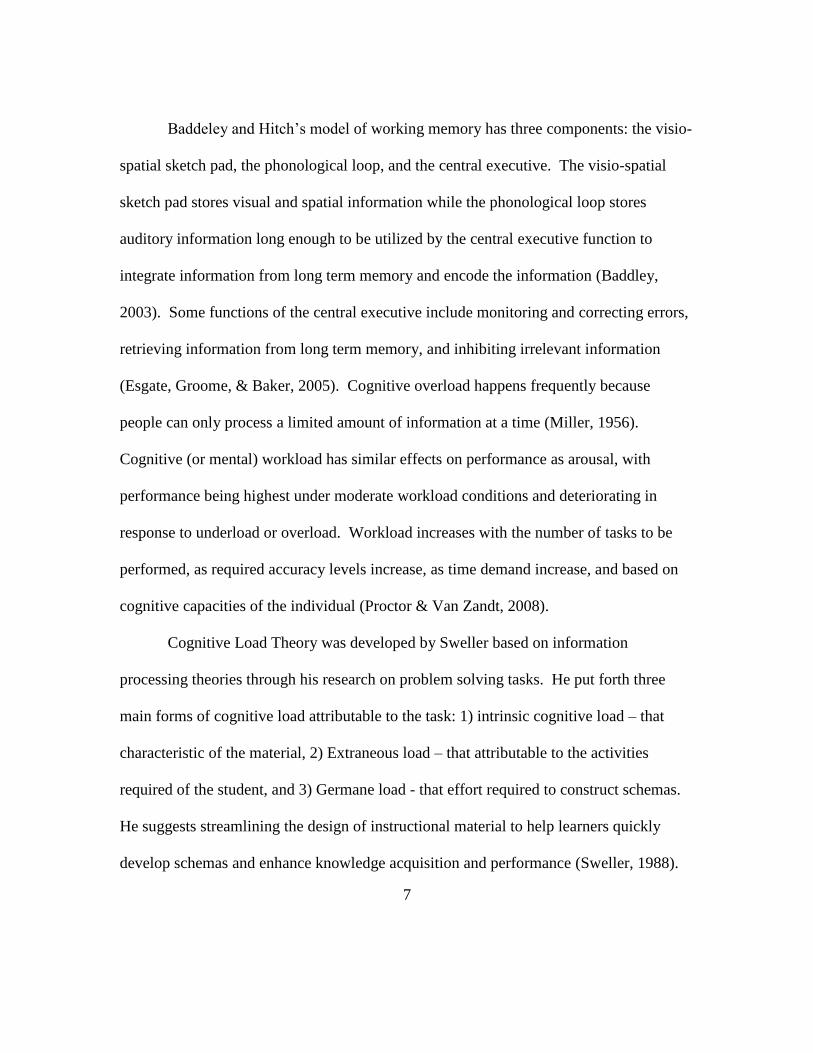
Baddeley and Hitch’s model of working memory has three components: the visio-

spatial sketch pad, the phonological loop, and the central executive. The visio-spatial

sketch pad stores visual and spatial information while the phonological loop stores

auditory information long enough to be utilized by the central executive function to

integrate information from long term memory and encode the information (Baddley,

2003). Some functions of the central executive include monitoring and correcting errors,

retrieving information from long term memory, and inhibiting irrelevant information

(Esgate, Groome, & Baker, 2005). Cognitive overload happens frequently because

people can only process a limited amount of information at a time (Miller, 1956).

Cognitive (or mental) workload has similar effects on performance as arousal, with

performance being highest under moderate workload conditions and deteriorating in

response to underload or overload. Workload increases with the number of tasks to be

performed, as required accuracy levels increase, as time demand increase, and based on

cognitive capacities of the individual (Proctor & Van Zandt, 2008).

Cognitive Load Theory was developed by Sweller based on information

processing theories through his research on problem solving tasks. He put forth three

main forms of cognitive load attributable to the task: 1) intrinsic cognitive load – that

characteristic of the material, 2) Extraneous load – that attributable to the activities

required of the student, and 3) Germane load - that effort required to construct schemas.

He suggests streamlining the design of instructional material to help learners quickly

develop schemas and enhance knowledge acquisition and performance (Sweller, 1988).

8

Sternberg’s Triarchic Theory of Human Intelligence builds on information

processing theories to describe analytical intelligence, the form of intelligence utilized in

problem solving. This theory breaks analytical intelligence into three components:

metacomponents, performance components, and knowledge acquisition components.

Metacomponents (i.e., metacognition) are higher-level central executive functions that

consist of planning, monitoring, and evaluating the problem solving process.

Performance components are the cognitive processes that complete operations in working

memory such as making calculations, comparing data, or encoding information.

Knowledge acquisition components are the processes used to gain or store new

knowledge in long term memory (Sternberg, 1985).

According to Mayer, there are three main cognitive processes utilized in

information processing during arithmetic type problem solving: selecting, organizing, and

integrating information (Mayer, 2008). Mayer also describes three kinds of cognitive

load associated with working memory processes: extraneous cognitive processing,

essential cognitive processing, and generative cognitive processing. Extraneous

cognitive processing is characterized by utilizing inappropriate approaches or using

irrelevant information. Essential cognitive processing involves the difficulty of material

compared to the knowledge base. Generative cognitive processing is affected by the

motivation of the students’ willingness to work to understand material. Mayer suggests

that educators should work to minimize extraneous processing, manage essential

processing, and foster generative processing (Mayer, 2008).

9

PROBLEM SOLVING THEORIES

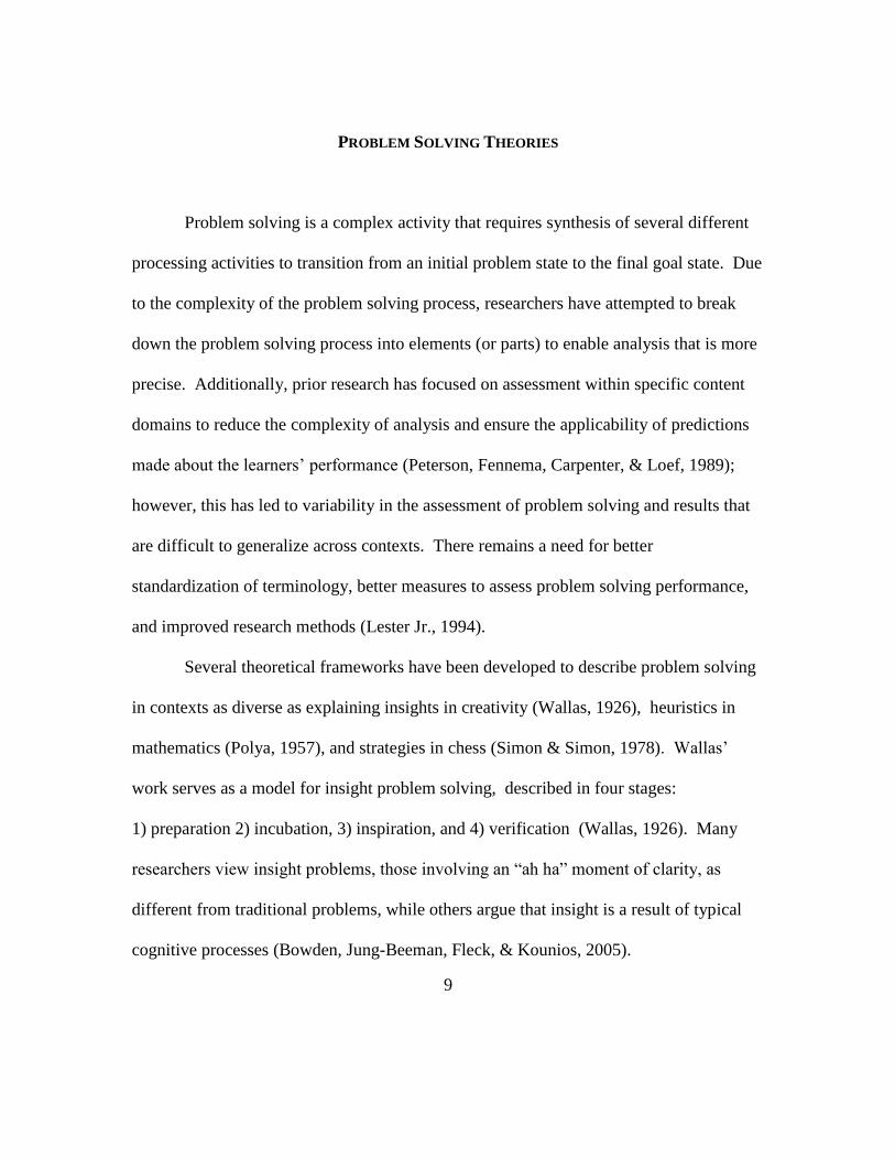
Problem solving is a complex activity that requires synthesis of several different

processing activities to transition from an initial problem state to the final goal state. Due

to the complexity of the problem solving process, researchers have attempted to break

down the problem solving process into elements (or parts) to enable analysis that is more

precise. Additionally, prior research has focused on assessment within specific content

domains to reduce the complexity of analysis and ensure the applicability of predictions

made about the learners’ performance (Peterson, Fennema, Carpenter, & Loef, 1989);

however, this has led to variability in the assessment of problem solving and results that

are difficult to generalize across contexts. There remains a need for better

standardization of terminology, better measures to assess problem solving performance,

and improved research methods (Lester Jr., 1994).

Several theoretical frameworks have been developed to describe problem solving

in contexts as diverse as explaining insights in creativity (Wallas, 1926), heuristics in

mathematics (Polya, 1957), and strategies in chess (Simon & Simon, 1978). Wallas’

work serves as a model for insight problem solving, described in four stages:

1) preparation 2) incubation, 3) inspiration, and 4) verification (Wallas, 1926). Many

researchers view insight problems, those involving an “ah ha” moment of clarity, as

different from traditional problems, while others argue that insight is a result of typical

cognitive processes (Bowden, Jung-Beeman, Fleck, & Kounios, 2005).

10

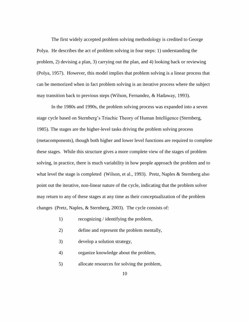
The first widely accepted problem solving methodology is credited to George

Polya. He describes the act of problem solving in four steps: 1) understanding the

problem, 2) devising a plan, 3) carrying out the plan, and 4) looking back or reviewing

(Polya, 1957). However, this model implies that problem solving is a linear process that

can be memorized when in fact problem solving is an iterative process where the subject

may transition back to previous steps (Wilson, Fernandez, & Hadaway, 1993).

In the 1980s and 1990s, the problem solving process was expanded into a seven

stage cycle based on Sternberg’s Triachic Theory of Human Intelligence (Sternberg,

1985). The stages are the higher-level tasks driving the problem solving process

(metacomponents), though both higher and lower level functions are required to complete

these stages. While this structure gives a more complete view of the stages of problem

solving, in practice, there is much variability in how people approach the problem and to

what level the stage is completed (Wilson, et al., 1993). Pretz, Naples & Sternberg also

point out the iterative, non-linear nature of the cycle, indicating that the problem solver

may return to any of these stages at any time as their conceptualization of the problem

changes (Pretz, Naples, & Sternberg, 2003). The cycle consists of:

1) recognizing / identifying the problem,

2) define and represent the problem mentally,

3) develop a solution strategy,

4) organize knowledge about the problem,

5) allocate resources for solving the problem,

11

6) monitor progress toward the goals, and

7) evaluate the solution for accuracy.

Greeno and Riley looked at the flow of information within the problem solving

process. The model of problem understanding and solution describes how the problem

solver must transform information from the problem text into problem schemata and then

an action schema before arriving at a solution. This model, illustrated in Figure 2.1,

identifies three stages to problem understanding 1) comprehension of the problem, 2)

mapping concepts to procedures, and 3) execution of procedures (Greeno & Riley, 1987).

Figure 2.1: Model of problem understanding and solution

Redrawn from (Greeno & Riley, 1987)

Other theories broaden the model of problem solving to include factors beyond

cognitive processing limitations, recognizing environmental/social factors and other

person factors. Kirton’s Cognitive Function Schema describes cognition as consisting of

three main functions, cognitive resources (including knowledge, skills, and prior

Problem

Schemata

Problem Text

Action

Schemata

Solution

Comprehension Execution

Mapping

12

experiences), cognitive affect (needs, values, attitudes, and beliefs), and cognitive effect

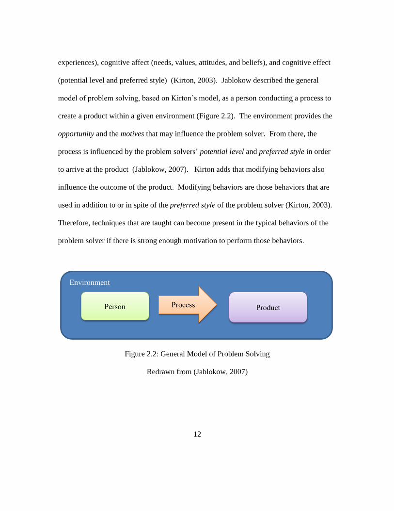
(potential level and preferred style) (Kirton, 2003). Jablokow described the general

model of problem solving, based on Kirton’s model, as a person conducting a process to

create a product within a given environment (Figure 2.2). The environment provides the

opportunity and the motives that may influence the problem solver. From there, the

process is influenced by the problem solvers’ potential level and preferred style in order

to arrive at the product (Jablokow, 2007). Kirton adds that modifying behaviors also

influence the outcome of the product. Modifying behaviors are those behaviors that are

used in addition to or in spite of the preferred style of the problem solver (Kirton, 2003).

Therefore, techniques that are taught can become present in the typical behaviors of the

problem solver if there is strong enough motivation to perform those behaviors.

Figure 2.2: General Model of Problem Solving

Redrawn from (Jablokow, 2007)

Environment

Person Process Product

13

FACTORS INFLUENCING PROBLEM SOLVING PERFORMANCE

A synthesis of research has shown that characteristics of the environment, such as

teaching style and problem difficulty; the person, such as prior knowledge; and the

process, such as cognitive and metacognitive tasks and strategies, influence problem

solving performance.

Characteristics of the Environment

The learning environment can have a great impact on a student’s ability to

develop process skills, such as problem solving. Instructors can promote skills

development by establishing a learning environment that provides practice applying the

skill, encourages monitoring and reflection, grades the process rather than just the

solution, utilizes standardized assessment and feedback, and teaches behaviors that have

been shown to promote successful application of the skill (Woods, et al., 2000).

Learning activities also need to be at an appropriate level that is challenging enough to

promote learning, but achievable so students do not get frustrated or doubt their abilities.

Funke described six features of a problem that contribute to its complexity (Funke, 1991):

1) Intransparency- lack of availability of information about the problem

2) Polytely- having multiple goals

3) Complexity of the situation- based on the number of variables and the type

of relationship between the variables

14

4) Connectivity of variables- the impact on variables due to a change in one

5) Dynamic developments- worsening conditions lead to time pressures

6) Time-delayed effects- one must wait to see the impact of changes

Extensive work by Jonassen defines various problem types and gives insight into

choosing appropriate problem types for the level of student and the outcomes being

assessed. For example, well-structured problems such as story problems are appropriate

for introducing students to new concepts and measuring arithmetic abilities, whereas ill-

structured problems such as design problems are more appropriate for measuring a

student’s ability to weigh alternatives and make comparative judgments among

alternative solutions (Jonassen & Hung, 2008). However, Pretz, Naples, & Sternberg

point out that the U.S. educational system’s overreliance on well-defined problems

causes students to be underexposed to practice using planning metacognitive processes of

recognizing, defining, and representing problems (Pretz, et al., 2003), which limits the

students development of these skills.

Characteristics of the Problem Solver

In much of problem solving research, the effectiveness of strategies is described

in terms of expert or novice performance. However, methods used by experts to solve

problems are not necessarily transferable to novices due to cognitive requirements of

using these strategies. For example, novices may have less knowledge on which to draw

conclusions and may experience an overload of cognitive resources when using expert

15

methods. Some of the major hindrances to achieving expert performance are the inability

to solve the problem without acquiring more information, lack of awareness of

performance errors, and resistance to changing a selected method or representation

(Wang & Chiew, 2010).

Expertise level has been used to explain many performance differences between

problem solvers. Novices commit more errors and have different approaches than

experts (Chi, Feltovich, & Glaser, 1981). Also, experts may be up to four times faster at

determining solutions than novices, even though experts also take time to pause between

retrieving equations or chunks of information (Chi, et al., 1981) and spend more time

than novices in the problem representation phase of the problem solving process (Pretz, et

al., 2003). Chess research showed that experts had better pattern recognition due to

larger knowledge bases developed through practice. Experts also organize their

information differently than novices, using more effective chunking of information than

novices (Larkin, Mcdermott, Simon, & Simon, 1980a), which is characteristic of higher

performing working memory. Research suggests that people can improve performance of

working memory by utilizing efficient processing techniques of selecting only relevant

information and organizing the information in chunks along with other strategies such as

writing down information to relieve cognitive demand (Matlin, 2001).

While it has been proposed that problem solving can be used to meet

instructional goals such as learning facts, concepts, and procedures (Wilson, et al., 1993),

research has shown that insufficient cognitive workload capacity may hinder learning

16

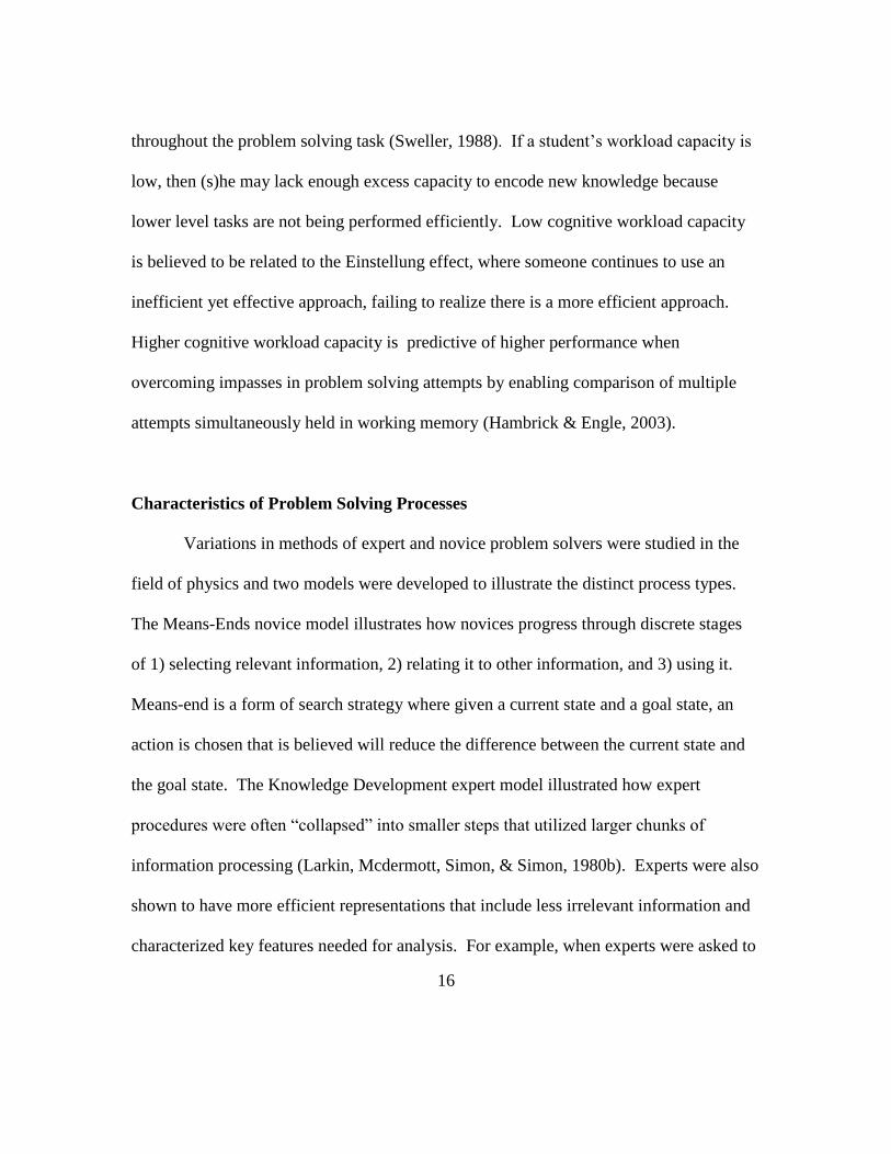
throughout the problem solving task (Sweller, 1988). If a student’s workload capacity is

low, then (s)he may lack enough excess capacity to encode new knowledge because

lower level tasks are not being performed efficiently. Low cognitive workload capacity

is believed to be related to the Einstellung effect, where someone continues to use an

inefficient yet effective approach, failing to realize there is a more efficient approach.

Higher cognitive workload capacity is predictive of higher performance when

overcoming impasses in problem solving attempts by enabling comparison of multiple

attempts simultaneously held in working memory (Hambrick & Engle, 2003).

Characteristics of Problem Solving Processes

Variations in methods of expert and novice problem solvers were studied in the

field of physics and two models were developed to illustrate the distinct process types.

The Means-Ends novice model illustrates how novices progress through discrete stages

of 1) selecting relevant information, 2) relating it to other information, and 3) using it.

Means-end is a form of search strategy where given a current state and a goal state, an

action is chosen that is believed will reduce the difference between the current state and

the goal state. The Knowledge Development expert model illustrated how expert

procedures were often “collapsed” into smaller steps that utilized larger chunks of

information processing (Larkin, Mcdermott, Simon, & Simon, 1980b). Experts were also

shown to have more efficient representations that include less irrelevant information and

characterized key features needed for analysis. For example, when experts were asked to

17

sort a series of physics problems, they grouped them based on the underlying theory

needed to solve the problem, where novices grouped them based on surface features of

the problems such as inclined planes (Chi, et al., 1988).

Another feature of problem solving performance is the level of metacognition

used to manage the problem solving process. MacGregor, Ormerod, and Chronicle’s

Progress Monitoring theory offers two models of approaches used to monitor

performance: 1) maximization heuristic, where problem solvers try to progress as far as

possible on each attempt or 2) progress monitoring, where problem solvers assess

progress toward the goal through incremental monitoring throughout the problem solving

process and redirect the approach after realizing it will lead to an incorrect solution

(Macgregor, Ormerod, & Chronicle, 2001). Problem solvers may fall to the

maximization heuristics if they lack the capacity to perform the procedures of the

progress monitoring model, which is more resource intensive.

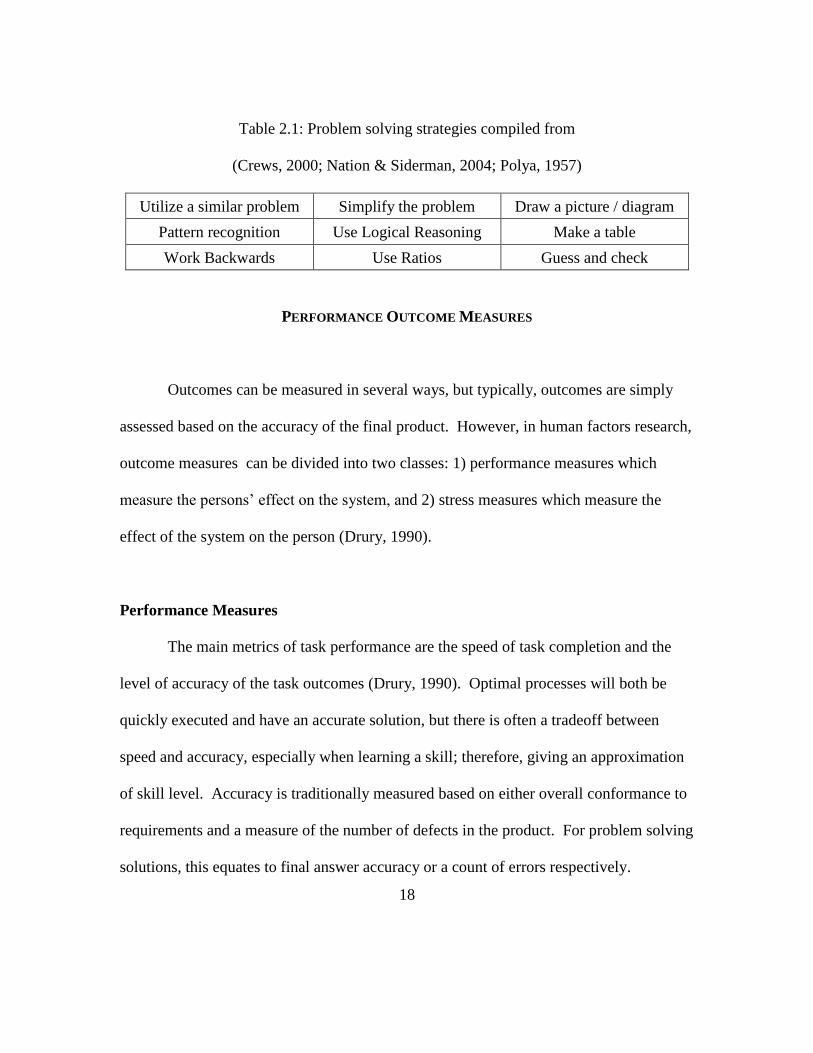
Since cognitive resources are limited, people utilize strategies and heuristics to

reduce cognitive load (Matlin, 2001). Table 2.1 shows a sample of strategies which have

been observed in arithmetic problem solving, though this is hardly a comprehensive list

(Crews, 2000; Nation & Siderman, 2004; Polya, 1957). While these strategies are useful

in reducing cognitive load, they are not useful in all situations and may lead to an

incorrect approach to solving the problem. Also people can become too reliant on

strategies or use them inappropriately, leading to a decrement in performance (Matlin,

2001).

18

Table 2.1: Problem solving strategies compiled from

(Crews, 2000; Nation & Siderman, 2004; Polya, 1957)

Utilize a similar problem Simplify the problem Draw a picture / diagram

Pattern recognition Use Logical Reasoning Make a table

Work Backwards Use Ratios Guess and check

PERFORMANCE OUTCOME MEASURES

Outcomes can be measured in several ways, but typically, outcomes are simply

assessed based on the accuracy of the final product. However, in human factors research,

outcome measures can be divided into two classes: 1) performance measures which

measure the persons’ effect on the system, and 2) stress measures which measure the

effect of the system on the person (Drury, 1990).

Performance Measures

The main metrics of task performance are the speed of task completion and the

level of accuracy of the task outcomes (Drury, 1990). Optimal processes will both be

quickly executed and have an accurate solution, but there is often a tradeoff between

speed and accuracy, especially when learning a skill; therefore, giving an approximation

of skill level. Accuracy is traditionally measured based on either overall conformance to

requirements and a measure of the number of defects in the product. For problem solving

solutions, this equates to final answer accuracy or a count of errors respectively.

19

Stress Measures

For cognitive tasks, the main stress measure is mental workload. There are

several ways of assessing mental workload including primary task measures, secondary

task measures, psychophysiological measures, and self-report assessments (Wilson &

Corlett, 2005). In the classroom environment, self-report assessments lend themselves as

the most practical measure based on their unobtrusive nature, ease of assessment, and

quick data collection. The three most widely used subjective measures of mental

workload are 1) the Modified Cooper-Harper scale, 2) NASA-Task Load Index (NASA-

TLX), and 3) Subjective Workload Assessment Technique (SWAT). All three

assessments are generic, can be applied to any domain, and are non- obtrusive to task

performance when administered after the task.

The Modified Cooper-Harper Scale assesses difficulty level on a ten-item scale

from very easy to impossible based on a classification of the demand level placed on the

operator. Accurate assessment utilizing this scale requires the operator to carefully read

each option and make fine distinctions between ratings of mental effort and ability to

thwart errors. For example, the operator must distinguish between ratings such as

“Maximum operator mental effort is required to avoid large or numerous errors” and

“Intense operator mental effort is required to accomplish task, but frequent or numerous

errors persist” (Wilson & Corlett, 2005). The Modified Cooper Harper scale cannot be

used to diagnose sources of workload stress and the reliability is dependent on the

operators acceptance and care to the task (Farmer & Brownson, 2003).

20

The NASA-TLX consists of six subscales, three measuring demand put on the

participant by the task and three measuring stress added by the worker as a result of

interacting with the task. The three measures of task demand include 1) mental demand,

2) physical demand, and 3) temporal demand. The remaining measures, 4) effort, 5)

performance, and 6) frustration, describe the stress put on the person by the interaction of

the person with the task (Warm, Matthews, & Finomore Jr., 2008). The NASA-TLX

subscales are scored on a continuous scale from zero to twenty (Stanton, Salmon, Walker,

Baber, & Jenkins, 2005). The NASA-TLX has been noted as highly reliable, extensively

validated, has a high sensitivity, can be used to diagnose sources of workload and takes

1-2 minutes to complete (Farmer & Brownson, 2003).

The SWAT is a three item scale that rates time load, mental effort load, and

psychological stress load on scales of 1-3. The scales do not easily translate to problem

solving activities though because the assessment is geared toward tasks that take

extensive time. For example, time load is measured on the three point scale: 1= Often

have spare time, 2=Occasionally have spare time, and 3=Almost never have spare time.

Additionally, SWAT has been criticized for being insensitive to low mental workloads

(Stanton, et al., 2005) and has not been empirically validated (Farmer & Brownson,

2003).

21

CHAPTER THREE

RESEARCH METHODS

RESEARCH DESIGN

This study utilizes mixed methods, executed using a concurrent nested strategy

for data collection. Concurrent nested strategies are characterized by data collection

phases where both qualitative and quantitative data are collected and the data is mixed

during analysis (Crewell, Plano Clark, Gutmann, & Loomis, 2003). In this study,

measures of prior academic experiences were collected at the beginning of the semesters,

followed by the collection of problem solutions, and, in Spring 2011, the collection of

surveys of perceived mental workload at three points throughout the semester. All data

was utilized concurrently in the evaluation of problem solving attempts and the impact of

person and process factors on problem solving performance.

EXPERIMENTAL DESIGN

A repeated measures experimental design was used to evaluate relationships

between predictive factors (participant and process) and outcome measures (accuracy,

efficiency, and workload measures) across a range of engineering contexts. The sample

group of students completed problem solving exercises three times.

22

Participants and Environment

First year engineering students enrolled in tablet sections of an engineering skill-

building course at Clemson, “Engineering Disciplines and Skills,” participated in this

research. Students used tablet computers in the classroom on a regular basis (once per

week, starting four weeks into the semester) to complete assignments using custom

software in lieu of paper submissions of their regular class assignments.

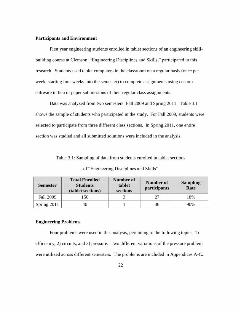
Data was analyzed from two semesters: Fall 2009 and Spring 2011. Table 3.1

shows the sample of students who participated in the study. For Fall 2009, students were

selected to participate from three different class sections. In Spring 2011, one entire

section was studied and all submitted solutions were included in the analysis.

Table 3.1: Sampling of data from students enrolled in tablet sections

of “Engineering Disciplines and Skills”

Semester

Total Enrolled

Students

(tablet sections)

Number of

tablet

sections

Number of

participants

Sampling

Rate

Fall 2009 150 3 27 18%

Spring 2011 40 1 36 90%

Engineering Problems

Four problems were used in this analysis, pertaining to the following topics: 1)

efficiency, 2) circuits, and 3) pressure. Two different variations of the pressure problem

were utilized across different semesters. The problems are included in Appendices A-C.

23

Problems needed to be structured enough for first year engineering students, but ill-

defined enough to elicit students’ problem-solving strategies upon analysis. Therefore,

all problems 1) had a constrained context, including pre-defined elements (problem

inputs), 2) allowed multiple predictable procedures or algorithms, and 3) had a single

correct answer. All problems were story problems, in which students were presented

with a narrative that embeds the values needed to obtain a final answer (Jonassen, 2010).

The first problem involved a multi-stage solar energy conversion system and

required calculation of the efficiency of one stage given input and output values for the

other stages. The second problem required students to solve for values of components in

a given electrical circuit. This problem, developed by the project team, also contained a

Rule-Using/Rule Induction portion (a problem having one correct solution but multiple

rules governing the process (Jonassen, 2010)), where students were asked to determine an

equivalent circuit based on a set of given constraints. The third problem involved total

pressure calculations for a pressurized vessel and required students to solve for values

within the system, and conversion between different unit systems.

DATA COLLECTION INSTRUMENTS

Four sources of data were collected from students: 1) solutions from three in-class

activities (Fall 2009 and Spring 2011), 2) a beginning of semester survey on academic

preparation (Fall 2009), and 3) the NASA-TLX for completed solutions (Spring 2011).

24

Problem Solutions Collected

Problem solving data were obtained via students’ completed solutions using a

program called MuseInk, developed at Clemson University (Bowman & Benson, 2010).

This software was used in conjunction with tablet computers that were made available to

all students during the class period. Students worked out problems in the MuseInk

application, which digitally records ink strokes. MuseInk files (.mi) keep a running log of

the entire problem solving process from beginning to end, including erasures, and can be

replayed. Student work can be coded directly in the application at any point in time

within the data file, thus allowing the researcher to associate codes to the problem

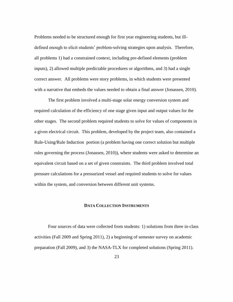
solution directly in the file, even in portions of the solution that had been erased. Not all

participants submitted solution files for every problem. Table 3.2 summarizes the

number of solutions collected from students.

Table 3.2: Number of problem solutions collected for each problem

Efficiency Problem Circuits Problem Pressure Problem

Fall 2009 24 22 22

Spring 2011 26 23 27

Total 50 45 49

Beginning of Semester Survey

At the beginning of each semester, a survey was sent out to all students enrolled

in this course. In Fall 2009, prior knowledge measures were obtained from open ended

25

responses to questions about a) previous mathematics courses and grades and b)

participation in any pre-engineering activities. For Fall 2009 and Spring 2011,

demographic information including gender and ethnicity was collected.

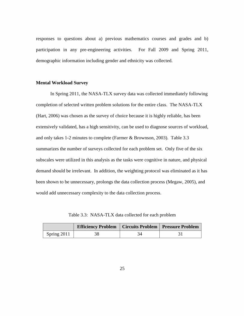
Mental Workload Survey

In Spring 2011, the NASA-TLX survey data was collected immediately following

completion of selected written problem solutions for the entire class. The NASA-TLX

(Hart, 2006) was chosen as the survey of choice because it is highly reliable, has been

extensively validated, has a high sensitivity, can be used to diagnose sources of workload,

and only takes 1-2 minutes to complete (Farmer & Brownson, 2003). Table 3.3

summarizes the number of surveys collected for each problem set. Only five of the six

subscales were utilized in this analysis as the tasks were cognitive in nature, and physical

demand should be irrelevant. In addition, the weighting protocol was eliminated as it has

been shown to be unnecessary, prolongs the data collection process (Megaw, 2005), and

would add unnecessary complexity to the data collection process.

Table 3.3: NASA-TLX data collected for each problem

Efficiency Problem Circuits Problem Pressure Problem

Spring 2011 38 34 31

26

DATA ANALYSIS METHODS

Data Transformation Methods

A task analysis approach was used to identify elements of the problem solving

process including tasks, strategies, errors, and answer states observed in student work.

The codes were generalized to tasks, strategies, and errors exhibited across various

engineering problem sets so that a consistent analysis method can be used for different

problems. Codes were assigned based on instances appearing within the work, where

strategy codes were assigned based on interpretation of the overall process for each

student’s work. The data from this coding process were then transformed into measures

believed to be indicators of problem solving skills level based on findings from the

literature. Then, mixed models were used to evaluate the solutions in terms of process

factors and performance measures while taking into account random factors attributed to

the participant. Chapter 4 is an in-depth account of the development of this coding

scheme. Chapter 5 is an extended description of the performance measures used in the

evaluation.

Statistical Analyses

While the experimental design makes use of repeated measures, the primary

interest is not the variation between problems and there is no attempt to assess gains

between trials. For that reason, analyses will be conducted in two ways. First, samples

27

were assessed as independent to identify and quantify any significant differences between

groups. Second, linear mixed models were used to evaluate the predictive power of

factors including effects of the problem on outcome measures of interest taking into

account random factors attributed to the participant. This is used as an alternative to the

repeated measures ANOVA as the rANOVA is highly vulnerable to effects of missing

data and unequal time points between subjects (Gueorguieva R, 2004).

Data of various types are evaluated throughout subsequent chapters, thus

requiring different statistical tests. The presence of a problem feature in a solution is of

the binomial data type. However, performance measures are of a variety of data types

including binomial and non-Gaussian types. Therefore, a variety of statistical tests were

utilized. These tests are summarized in Table 3.4 and explained briefly below.

Table 3.4: Summary of statistical tests by data type

Binomial Score

(Two Possible Outcomes)

Measurement

(Non- Gaussian Population)

Compare two unpaired

groups

Chi-square

goodness of fit test

Wilcoxon Rank Sum (Mann-

Whitney test)

Quantify association

between two variables Odds ratios Spearman correlation

Predict value from

several measured or

binomial variables

Multiple logistic regression Multiple linear regression

28

Chi Squared Test: A Chi-square test is used to test how likely an observed

distribution is due to chance. It is used to analyze categorical (binomial) data and

evaluate whether there is a difference in population proportions (Gravetter & Wallnau,

2008). This analysis was used to assess whether the use of specific tasks, errors, and

strategies differ between groups

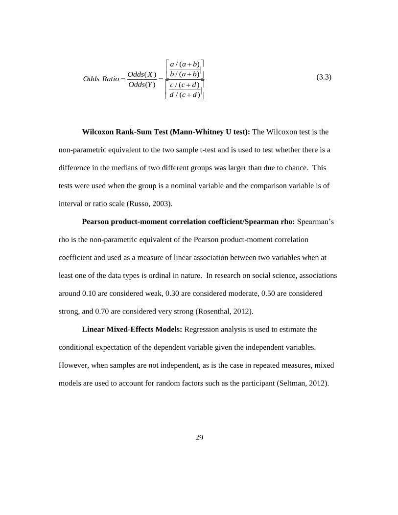
Odds Ratios: To assess the likelihood of a an event occurring given another

factor, odds ratios were calculated using a 2x2 contingency table depicting the number of

cases in which an event occurs and does not occur for two mutually exclusive populations

(Sheskin, 2004). Table 3.5 illustrates a sample contingency table, calculations 3.1-3.3

detail how to compute an odds ratio. This analysis was used to assess the magnitude by

which the use of specific tasks, errors, and strategies differ between groups.

Table 3.5: Sample Contingency Table: odds ratios >1 indicate more likely events.

Obtain a correct answer (1) Do not obtain a correct answer (0)

Males (X) a b

Females (Y) c d

( ) / ( )( )

( ) / ( )

p X will occur a a bOdds X

p X will not occur b a b

(3.1)

( ) / ( )( )

( ) / ( )

p Y will occur c c dOdds Y

p Y will not occur d c d

(3.2)

29

/ ( )

/ ( )( )

( ) / ( )

/ ( )

a a b

b a bOdds XOdds Ratio

Odds Y c c d

d c d

(3.3)

Wilcoxon Rank-Sum Test (Mann-Whitney U test): The Wilcoxon test is the

non-parametric equivalent to the two sample t-test and is used to test whether there is a

difference in the medians of two different groups was larger than due to chance. This

tests were used when the group is a nominal variable and the comparison variable is of

interval or ratio scale (Russo, 2003).

Pearson product-moment correlation coefficient/Spearman rho: Spearman’s

rho is the non-parametric equivalent of the Pearson product-moment correlation

coefficient and used as a measure of linear association between two variables when at

least one of the data types is ordinal in nature. In research on social science, associations

around 0.10 are considered weak, 0.30 are considered moderate, 0.50 are considered

strong, and 0.70 are considered very strong (Rosenthal, 2012).

Linear Mixed-Effects Models: Regression analysis is used to estimate the

conditional expectation of the dependent variable given the independent variables.

However, when samples are not independent, as is the case in repeated measures, mixed

models are used to account for random factors such as the participant (Seltman, 2012).

30

CHAPTER FOUR:

DESIGN AND VALIDATION OF A CODING SCHEME FOR ANALYZING

ENGINEERING PROBLEM SOLVING

This study introduces a coding scheme for analyzing problem solutions in terms

of cognitive and metacognitive processes and problem solving deficiencies for first year

engineering students. The coding scheme is presented with the development process,

which may serve as a reference for other researchers analyzing complex tasks. A task

analysis approach was used to assess students’ problem solutions. A theoretical

framework from mathematics research was utilized as a foundation to categorize the set

of elements. The resulting coding scheme is comprised of 54 codes within the categories

of knowledge access, knowledge generation, self-management, conceptual errors,

mechanical errors, management errors, approach strategies, and solution accuracy. Inter-

rater reliability (Cohen’s Kappa) for two of the original coders was 0.769 for all coded

elements and 0.942 when adjusted to assess agreement only on elements coded by both

coders. The coding scheme was demonstrated to be reliable and valid for analyzing

problems typical of topics in first year engineering courses. Task analyses allow the

problem solving process to be evaluated in terms of time, process elements, errors

committed, and self-corrected errors. Therefore, problem solving performance can be

analyzed in terms of both accuracy and efficiency of processing, pinpointing areas

meriting further study from a cognitive perspective, as well as areas of instructional need.

31

INTRODUCTION

In engineering professions, an important skill set to possess is accurate and

efficient problem solving. While engineers once worked almost exclusively in their field

of study, the practice of engineering is changing in the wake of a rapidly changing global

economy. Companies are faced with new challenges that require integration of

knowledge from various domains, and are often under tight time constraints to find

solutions (National Academy of Engineering, 2004). Therefore, proficiency in problem

solving is even more valuable as industry looks to engineers to tackle problems involving

such constraints as technological change (Jablokow, 2007), market globalization, and

resource sustainability (Rugarcia, et al., 2000). The National Academy of Engineers

describes the necessary attributes of the engineer of 2020 as having ingenuity, problem

solving capabilities, scientific insight, creativity, determination, leadership abilities,

conscience, vision, and curiosity (2004).

In order to prepare for problem solving in the workplace, students must develop

conceptual and procedural frameworks that they can use to solve real world problems that

are often complex, have conflicting goals, and undefined system constraints (Jonassen, et

al., 2006). However, students must first build an engineering knowledge base and

develop process skills used in the application of knowledge such as problem solving and

self-assessment (Woods, et al., 2000). Because of the importance of problem solving

skills, educators should strive to help students obtain the knowledge resources and

32

develop process skills required for problem solving success. In order to assess the

development of problem-solving skills, it is necessary to be able to assess students’

performances on a common set of criteria at various points in their studies.

The purpose of this research is to establish a standardized method for analyzing

problem solutions in terms of characteristics that have been shown to indicate differences

in skill level. This paper details the methodology used to develop a structured scheme for

coding the solution processes of first year engineering students solving engineering

problems independently, and presents the coding scheme as a valid instrument for

assessing first year engineering students’ problem solving skills using a mixed model

methodology. For information on mixed model methodologies, see (Tashakkori &

Teddlie, 1998).

LITERATURE REVIEW

Much research has been conducted on problem solving from a variety of

perspectives. This review of relevant literature first describes the various models that

have been proposed to explain the problem solving process, and then describes some of

the factors that have been shown to impact problem solving success in the educational

problem solving context.

33

Problem Solving Models

Several theoretical frameworks describe problem solving in contexts as diverse as

explaining insights in creativity (Wallas, 1926), to heuristics in mathematics (Polya,

1957), and gaming strategies in chess (Simon & Simon, 1978). Wallas’ model of

problem solving serves as a model for insight problem solving, and describes creative

problem solving in four stages: 1) preparation 2) incubation, 3) inspiration, and 4)

verification (Wallas, 1926). The first widely-accepted problem solving methodology is

credited to George Polya, who describes the act of problem solving in four steps: 1)

understanding the problem, 2) devising a plan, 3) carrying out the plan, and 4) looking

back or reviewing (Polya, 1957). However, like other heuristic models, the implication

that problem solving is a linear process that can be memorized is flawed; problem solvers

may iteratively transition back to previous steps (Wilson, et al., 1993).

A more recent model depicts problem solving as a seven stage cycle that

emphasizes the iterative nature of the cycle (Pretz, et al., 2003). The stages include: 1)

recognize / identify the problem, 2) define and represent the problem mentally, 3)

develop a solution strategy, 4) organize knowledge about the problem, 5) allocate

resources for solving the problem, 6) monitor progress toward the goals, and 7) evaluate

the solution for accuracy. While this structure gives a more complete view of the stages

of problem solving, in practice, there is much variability in how people approach the

problem and how well each of the stages are completed, if at all (Wilson, et al., 1993).

The stages listed above are based on Sternberg’s Triarchic Theory of Human

34

Intelligence, which breaks analytical intelligence, the form of intelligence utilized in

problem solving, into three components: metacomponents, performance components, and

knowledge acquisition components. Metacomponents (metacognition) are higher-level

executive functions consisting of planning, monitoring, and evaluating the problem

solving process. Performance components are the cognitive processes that perform

operations such as making calculations, comparing data, or encoding information.

Knowledge acquisition components are the processes used to gain or store new

knowledge (Sternberg, 1985). The planning phase of the problem solving process

consists of executive processes including problem recognition, definition, and

representation (Pretz, et al., 2003). Pretz, Naples, & Sternberg point out that the

educational system typically uses well-defined problems and therefore students may be

underexposed to practice using planning metacognitive processes of recognizing,

defining, and representing problems (Pretz, et al., 2003).

Other theories broaden the scope of factors influencing problem solving by

recognizing environmental/social factors and other person factors beyond cognitive

processing of knowledge. Kirton’s Cognitive Function Schema describes cognition as

consisting of three main functions, cognitive resources (including knowledge, skills, and

prior experiences), cognitive affect (needs, values, attitudes, and beliefs), and cognitive

effect (potential level and preferred style) (Kirton, 2003). The environment provides the

opportunity and the motives that may influence the problem solver. From there, the

process is influenced by the problem solvers’ potential level and preferred style in order

35

to arrive at the product (Jablokow, 2007). Kirton adds that modifying behaviors also

influence the outcome of the product. Modifying behaviors are those behaviors that are

used in addition to or in spite of the preferred style of the problem solver (Kirton, 2003).

Therefore, techniques that are taught can become present in the typical behaviors of the

problem solver if there is strong enough motivation to perform those behaviors.

Factors Influencing Problem Solving Success

Research in problem types and strategies has shown that characteristics of the

problem such as the complexity or structure of the problem (Jonassen & Hung, 2008),

the person such as prior experiences (Kirton, 2003) and reasoning skills(Jonassen &

Hung, 2008), the process such as cognitive and metacognitive actions (Greeno & Riley,

1987; Sternberg, 1985) and strategies (Nickerson, 1994), and the environment such as the

social context (Woods, et al., 2000) influence problem solving performance.

In the search for behaviors that promote proficiency in problem solving, much

research has focused on classifying variations in performance between expert and novice

problem solvers (Hutchinson, 1988) presumably because expert problem solutions exhibit

more successful application of problem solving skills. Expertise level has been used to

explain many performance differences between problem solvers. For example, research

has shown that novices commit more errors and have different approaches than experts

(Chi, et al., 1981). Experts have been shown to be up to four times faster at determining

a solution than novices, even though experts also take time to pause between retrieving

36

equations or chunks of information (Chi, et al., 1981) and spend more time than novices

in the problem representation phase of the problem solving process (Pretz, et al., 2003).

Experts also organize their information differently than novices, displaying larger

chunking of information than novices (Larkin, et al., 1980a).

However, methods used by experts to solve problems are not necessarily

transferable to novices due to cognitive requirements necessary to use these strategies.

Cognitive overload may be a factor in some of the major hindrances to achieving

proficiency including the inability to solve the problem without acquiring more

information, lack of awareness of performance errors, and resistance to changing a

selected method or representation (Wang & Chiew, 2010). Various strategies can be

used in solving problems that alleviate some of the cognitive demand required by the

problem, such as problem decomposition or subgoaling (Nickerson, 1994); however,

people can become too reliant on strategies or use them inappropriately, leading to a

decrement in performance (Matlin, 2001).

Less emphasis has been given to determining how to assess the development of

problem solving skills. As Lester describes, there remains a need for better

standardization of terminology used, better measures to assess problem solving

performance, and improved research methods (Lester Jr., 1994).

37

METHODS

The objectives of this paper are twofold: 1) to describe the methodology used to

develop a coding scheme such that it can serve as a guide to other researchers who seek

to develop methods to analyze complex tasks, and 2) to present the coding scheme itself,

which may be used by education researchers or instructors who wish to analyze problem

solving in similar contexts. The coding scheme is used to analyze solutions from a

variety of problems typical of an introductory engineering course. By analyzing multiple

students’ problem solving attempts, we can identify common variations in process types

and evaluate the effect of person and process factors on problem solving performance.

However, in order to enable comparison of processes across problem types, there must be

a standardized means of analysis.

Educational Environment

Problem solutions were collected from first year engineering students in an

introductory engineering course that is taught in a “studio” setting using active

cooperative learning techniques. While students are regularly encouraged to work with

their peers on in-class activities, students completed the problems in this study

independently. Students in the course sections taught by a member of the research team

were invited to participate in this study. Data was collected from 27 students; however

not all students completed all three problems analyzed. In addition to problem solutions,

38

other data collected from participants included demographics, and academic preparation

before college enrollment (math and science courses taken, grades in those courses, and

pre-college engineering activities or courses).

Engineering Problem Types

For this analysis, problems were chosen based on characteristics that would

ensure moderate problem difficulty for students in a first year engineering classroom,

who are building their engineering knowledge base and process skills. The chosen

problems struck a balance of being well-structured enough to limit the cognitive load on

the students, but remain challenging and provide multiple perspectives to solving the

problem in accordance with the guidelines for problem-based learning (Jonassen & Hung,

2008). All problems had 1) a constrained context, including pre-defined elements

(problem inputs), 2) allowed multiple predictable procedures or algorithms, and 3) had a

single correct answer (Jonassen, 2004). Three problems were selected that reflected a

variety of types of well-structured problems. Two originated from the course textbook

(Stephan, Sill, Park, Bowman, & Ohland, 2011) and one was developed by the project

team. All three problems were story problems, in which the student is presented with a

narrative that embeds the values needed to obtain a final answer (Jonassen, 2010). The

first problem involved a multi-stage solar energy conversion system and required

calculation of the efficiency of one stage given input and output values for the other

stages (Appendix A). The second problem required students to solve for values of

39

components in a given electrical circuit (Appendix B). This problem, developed by the

project team, also contained a Rule-Using/Rule Induction portion (a problem having one

correct solution but multiple rules governing the process (Jonassen, 2010)), where

students were asked to determine an equivalent circuit based on a set of given constraints.

The third problem involved total pressure calculations and required students to solve for

values within the system, and conversion between different unit systems (Appendix C).

Tablet PC Technology and Data Collection Software

In order to capture problem-solving processes for analysis, students wrote their

solution attempts on a Tablet PC using a custom-designed software called MuseInk

(Bowman & Benson, 2010; Grigg & Benson, 2011). The software allows students to

work problems on a Tablet PC, and stores the digital Ink in such a way that it can be

played back, annotated, and exported to a database where the data can be queried for

analysis. Students work through problems much as they would with pen and paper, with

the added benefit of having electronic access to their work, while researchers are

provided with a comprehensive expression of the problem solving attempt from

beginning to end including work that was erased in the process.

Analysis Methods

While several researchers have developed independent coding schemes to aid in

the analysis of problem solving, most researchers have analyzed written work in

40

conjunction with a think-aloud (Artzt & Armour-Thomas, 1992; Litzinger, et al., 2010;

Weston, et al., 2001; Wong, Lawson, & Keeves, 2002). These coding schemes are

tailored to analyze the students’ verbal expressions of their work and not the elements

explicitly contained in the artifact itself, i.e. the students’ actual problem solution by

which they communicate their problem solving competencies in the classroom. Coding

schemes for assessing students’ think-alouds are not readily applicable to the assessment

of the written problem solutions. Yet, written data is rich in many ways, and analyzing

tasks explicitly enacted under authentic problem solving conditions can reveal strategies

or errors that occur organically and that may impact problem solving success.

A task analysis approach was utilized in order to develop a taxonomy of

component and subcomponent tasks involved in problem solving solutions, along with a

taxonomy of errors and strategies used by first year engineering students. Task analysis

methods originate with the work of Gilbreth (Gilbreth, 1914) and Taylor (Taylor, 1911),

whose work-study approaches were traditionally used to evaluate and improve the

efficiency of workers (Stammers & Shepherd, 1990). The definition of task analysis has

been broadened to include the qualitative assessment of humans interacting with a system

or process in order to understand how to better match the demands of the task to the

capabilities of the human (Wickens, Gordon, & Liu, 1998). The subcomponent tasks

obtained from task analyses, referred to as elements, often serve as inputs for other forms

of data analysis including error analysis and process charting techniques (Stanton, et al.,

2005). Research in mathematics education describes the importance of error analysis as

41

providing the opportunity to diagnose learning difficulties and develop criteria for

differentiating education, so that instructors can tailor education to individual students in

order to improve their performance and understanding (Radatz, 1980). While there is no

consensus on what constitutes an element, typically they are defined as discrete,

measureable, and repeatable units of activity, and it is at the researcher’s discretion to

assign elements that are appropriately sized for the intended analysis (Stammers &

Shepherd, 1990).

CODING SCHEME DEVELOPMENT

The remainder of this paper describes the method used to develop a taxonomy of

codes that will be used to analyze engineering problem solutions and validate the coding

scheme against current literature.

1. Form an Interdisciplinary Team of Coders to Scrutinize the Coding Scheme

In order to ensure high quality codes, an interdisciplinary team was formed to

assess problem solving solutions so that the coding scheme could undergo a high level of

scrutiny from several different perspectives. The interdisciplinary team was made up of

two faculty members, an instructor, and a graduate student. One faculty member

instructs in engineering education as well as in a first year engineering program, with a

background in bioengineering. The other faculty member is an instructor in secondary

42

science education with a background in cognitive science. One team member was an

instructor in a first year engineering program with a background in computer engineering.

The graduate student was a lab instructor in industrial engineering with a background in

human factors engineering. The variety of disciplines represented in the group allowed

the team to refine codes to the language of the engineer that was generic enough to be

applicable in a range of engineering topics.

2. Determine Requirements of the Coding Scheme

The long-term goal of our research is to examine the impact of prior academic

experiences and process variations (such as cognitive skills, metacognitive skills, and

strategies) on problem solving performance for engineering students. The coding scheme

had to enable analysis of problem solutions in accordance with our variables of interest.

Therefore, it had to distinguish between students drawing information from their prior

knowledge, and students drawing information from the problem text. It also needed to

distinguish between manipulating information for the purposes of solving the problem

(cognitive tasks) and for the purposes of self-correcting (metacognitive tasks).

We also wanted to ensure that problem solving performance could be evaluated

utilizing the information obtained using the coding scheme. Jonassen suggests a six item

rubric of criteria to evaluate performance of story problems: 1) accuracy of problem

classification, 2) identification of initial conditions, 3) accuracy of equations, 4) accuracy

of answer estimate, 5) unit consistency, and 6) accuracy of answer (Jonassen, 2004).

43

However, these criteria only assess the accuracy of information gathered from the

problem text and other resources, and solution accuracy. Our study looks at how well (if

at all) students identify and correct errors (inconsistent units, incorrect equations,

incorrect initial conditions, etc.) in addition to the accuracy of the solution.

3. Develop an Initial Coding Scheme

Once the requirements for the coding scheme were established, an appropriate

structure for the coding scheme was identified. While there are several different

approaches to creating a coding scheme, we utilized an a priori framework as a starting

point and modified codes to fit our task and population. Researchers may wish to utilize

a coding scheme as is or develop a new one from scratch using grounded theory

(Hutchinson 1988). The choice depends on the availability of preexisting coding

schemes to meet the research objectives.

We identified four major components necessary for our coding scheme: 1)

process elements, 2) errors, 3) approach strategies, and 4) solution accuracy. The

majority of the problem solving solution is coded through identifying process elements

and errors if they are present. Approach strategy and final answer accuracy are

classifications of the solution as a whole, and will only be coded at the end of the solution

(or at the end of each part for multi-part problems).

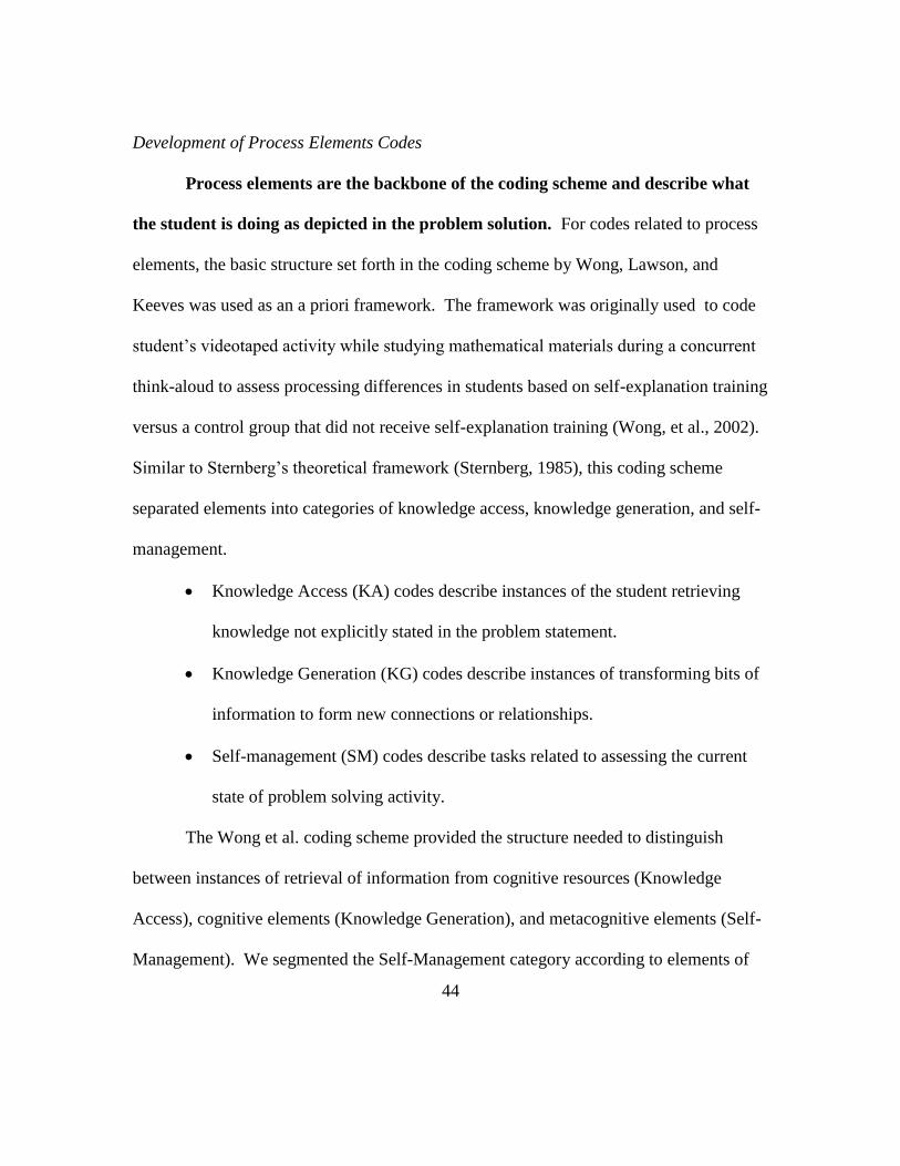
44

Development of Process Elements Codes

Process elements are the backbone of the coding scheme and describe what

the student is doing as depicted in the problem solution. For codes related to process

elements, the basic structure set forth in the coding scheme by Wong, Lawson, and

Keeves was used as an a priori framework. The framework was originally used to code

student’s videotaped activity while studying mathematical materials during a concurrent

think-aloud to assess processing differences in students based on self-explanation training

versus a control group that did not receive self-explanation training (Wong, et al., 2002).

Similar to Sternberg’s theoretical framework (Sternberg, 1985), this coding scheme

separated elements into categories of knowledge access, knowledge generation, and self-

management.

Knowledge Access (KA) codes describe instances of the student retrieving

knowledge not explicitly stated in the problem statement.

Knowledge Generation (KG) codes describe instances of transforming bits of

information to form new connections or relationships.

Self-management (SM) codes describe tasks related to assessing the current

state of problem solving activity.

The Wong et al. coding scheme provided the structure needed to distinguish

between instances of retrieval of information from cognitive resources (Knowledge

Access), cognitive elements (Knowledge Generation), and metacognitive elements (Self-

Management). We segmented the Self-Management category according to elements of

45

planning, monitoring, evaluating, and revising the solution in accordance to Hartman’s

definition of the executive management aspects of metacognition (Hartman, 2001).

Development of Error Codes

Error codes indicate instances where a problem first occurs; errors always

occur in conjunction with a process element. For codes relating to errors, we utilized a

structure derived from error detection literature in accounting, where it is common to

classify errors as conceptual and mechanical errors (Owhoso, Messier, & Lynch Jr.,

2002; Ramsay, 1994).We added a category for management errors to capture errors in

metacognitive processes.

Conceptual errors describe instances of misunderstanding of the problem

and/or underlying fundamental concepts

Mechanical errors describe instances of operation errors like miscalculations

Management errors describe instances of mismanaging information including

identify given information, transcribing values, or erasing correct work.

With this error coding structure, an improper equation selection or a flawed

version of the correct equation would be classified as a conceptual error, but misusing a

proper equation such as incorrectly manipulating an equation would be classified as a

mechanical error. In this way, errors related to students’ understanding of engineering

concepts and their computational skills can be identified separately. This allows

researchers to pinpoint hindrances to learning. For example, the case in which a student

46

does not use the efficiency equation properly because s/he did not understand the concept

of efficiency is a much different case than if the student erred in using the equation

because s/he has difficulty manipulating equations due to weak algebra skills or

inattention to details.

Development of Strategy Codes

Strategy codes are one time use codes that describe the overall approach

taken to solve the problem. For strategy codes, we utilized a subset of strategies that

appeared most applicable to story problems from the compilation described in “Thinking

and Problem Solving” (Nickerson, 1994). The subset was refined from the broader list of

strategies identified by Nickerson over the course of reviewing multiple problems

completed by different students with different academic backgrounds.

Development of Solution Accuracy Codes

Solution accuracy codes are one time use codes that describe the accuracy of

the final answer. While standard answer states of “correct” and “incorrect” could be

used to describe the accuracy of the problem solution, two additional codes were included

to further describe solutions: “Correct but Missing/Incorrect units”, and “Gave up”.

These two codes are subsets of the Correct and Incorrect solutions respectively.

Solutions coded as “Correct but Missing/Incorrect Units” are solutions in which the

numerical value of the solution is correct, but the units are missing or the answer is given

47

in a unit other than what was required, such as 120 seconds when the correct answer

should have been reported in minutes. The code “Gave up” indicates that no final answer

was obtained.

4. Establish a Coding Protocol

It is important to establish a protocol for how and where to assign codes to ensure

consistency between coders. For the purposes of our research, the task of solving an

engineering problem was broken down into discrete elements based on apparent changes

in action such as transitions between identifying information from the problem statement,

identifying information from their resources, manipulating information, and revising

work. One unique function of the tablet-based software developed for this project,

MuseInk, is that codes inserted in the work show up on the solution space, attached to a

stroke within the solution like a map tack. This enables the code to be mapped to a

specific point in the problem solving process. However, in order to use this feature most

efficiently, it is important to code precisely at the point in time where the stroke is in

order to avoid confusion when interpreting the data. To make best use of this

functionality, it was established that all codes should be assigned at the end of an element

for consistency. This also established a method for determining time between

completions of activities. Additionally, it was determined that every erasure except

correcting penmanship should be coded. Figure 4.1 depicts a snapshot of a code that is

placed on a process element.

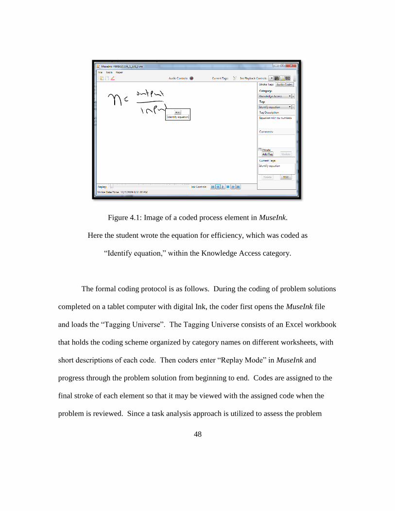
48

Figure 4.1: Image of a coded process element in MuseInk.

Here the student wrote the equation for efficiency, which was coded as

“Identify equation,” within the Knowledge Access category.

The formal coding protocol is as follows. During the coding of problem solutions

completed on a tablet computer with digital Ink, the coder first opens the MuseInk file

and loads the “Tagging Universe”. The Tagging Universe consists of an Excel workbook

that holds the coding scheme organized by category names on different worksheets, with

short descriptions of each code. Then coders enter “Replay Mode” in MuseInk and

progress through the problem solution from beginning to end. Codes are assigned to the

final stroke of each element so that it may be viewed with the assigned code when the

problem is reviewed. Since a task analysis approach is utilized to assess the problem

49

solving solution in terms of process, a new code is assigned for each transition in process

(Konz & Johnson, 2004). Therefore, each segment of work is coded with one process

element code and error codes are only assigned in association with a process element

code. No error codes were assigned without an associated process element code.

5. Pilot test the Coding Process

Problem solutions for three students were selected at random (n = 24) from the

solar efficiency problem for initial coding. One member of the research team initially

reviewed the three solutions and began classifying processing elements present in the

work within the KA, KG, and SM categories. Once an initial classification of problem

solving processing elements was developed, the interdisciplinary team of researchers met

to discuss the grouping of codes and ensure that 1) the codes were appropriate

descriptions of the elements, 2) they were general enough to be applied to other

problems, and 3) they were categorized appropriately according to the theoretical

framework. In this collaborative session, the description of process elements was

displayed in a spreadsheet on an overhead projector while the group verified the correct

classification of each code one by one in accordance with the theoretical framework

(Wong, et al., 2002), making changes as deemed appropriate. Ideas and concerns over

potential changes to the codes were documented by writing notes directly on the

spreadsheet using a tablet computer. A code book was established to define codes,

describe how each code was to be used, provide contrasts with related codes that could be

50

misinterpreted, and give examples. Coders can refer to the code book to ensure that

developed procedures are followed consistently. Once a consensus was formed on codes,

three members of the interdisciplinary team (those with engineering backgrounds) coded

the three selected solutions. For the first round of coding, coders assigned codes

independently and then reconvened to determine coding agreement.

6. Assess Reliability of the Coding Protocol

In order to evaluate the validity of the coding protocol and inter-rater reliability

for the three coders, coded solutions were assessed on three criteria: 1) code agreement

(i.e., Did all coders associate this particular code with the element?), 2) code frequency

(i.e., Did all coders code the same number of elements?) and 3) code timing (i.e., Were

elements coded by coders consistently at the same point within a solution, namely within

five ink strokes of one another?).

Inter-rater reliability was calculated based on overall agreement rates for all coded

elements as shown in calculation (1) and adjusted overall agreement rate for only

elements coded by all coders as shown in calculation (2) (Gwet, 2010).

Overall Agreement Rate = # ratings in agreement / total # of ratings (1)

Adjusted Overall Agreement Rate =

# ratings in agreement / (total # of ratings - # of ratings with missing data) (2)

51

“Agreement” was defined as an instance where a code was identified by all

coders. “Missing data” was defined as an element that one coder applied a code to but

another did not, which may be considered an important omission. In this study, inter-

rater agreement was calculated both ways. Overall agreement (inclusion of missing data)

answers the question, “To what degree do coders identify elements the same way?” This

approach examines the degree to which coders can both identify elements and code

elements accurately, and that the codes are sufficient for describing student problem

solving. Adjusted overall agreement (dropping missing codes from the analysis) answers

the questions, “To what degree are the codes sufficient for describing student problem

solving? Given a set of identified elements, do two coders code elements similarly?”

These questions examine the degree to which the codes sufficiently describe student work

(validity of the coding system), and are reliably applied. While dropping missing data

from the analysis reveals if coders are applying the same codes, such analysis does not

account for the case in which actually identifying elements is an important part of the

coding process. Therefore, missing data may be dropped from analysis to examine the

codes and their application, but missing data should be retained for understanding the

whole coding process that coders use in analyzing student work. An instance where

coders fail to identify an element and apply a code signals a need for better coder

training, or collapsing of codes so they are less specific and can be more broadly applied.

In contrast, an instance of disagreement about what a code means might indicate that

additional clarity around the meaning and interpretation of the codes is required.

52

Initial inter-rater reliability was calculated by examining only overall agreement

(including missing data), to assess the whole coding process. Results showed an overall

agreement rate of 55%, with individual agreement rates of 77%, 55%, and 42% for the

three solutions. Reviewing the instances of disagreements was instrumental in

identifying inconsistencies in applying codes and revealing missing problem solving

features that were not captured in the initial coding scheme.

7. Iteratively Refine the Coding Scheme and Protocol

Two more iterations of revisions were conducted before reaching a satisfactory

level of inter-rater reliability. For the second round of coding, three new students’

solutions were coded and overall agreement calculated. Using the scoring classifications

described in (Gwet, 2010), initial inter-rater reliability for the second round was

“Moderate” with overall agreement lower than the initial round of coding (for the three

solutions, inter-rater agreement was 73%, 40%, and 25%, for an overall agreement rate of

41%). This round of coding revealed that, with the addition of new codes and

reconfiguring code categories, there was confusion with the use of specific codes as well

as the frequency of assigning codes. The coding protocol was clarified and documented

in the codebook. In order to improve the inter-rater reliability of coders, a round-robin

review cycle was implemented for the next round of coding, in which each coded

problem was reviewed by a second coder in order to perform an internal check of

adherence to proper coding procedures.

53

During the next iteration, each rater coded three new students’ solutions, and then

reviewed coded data from one of the other two raters. In the case of discrepancies

between raters (code reviewers identified codes that should be added or deleted),

comments were added identifying the reviewer and the suggested action. Then the

original rater reviewed the suggested changes and accepted or rejected them. The process

whereby each submission was coded by each rater, then reviewed by another rater

provided an intense learning session for the raters, which helped establish the final coding

protocol.

The third round of coding showed greatly improved overall agreement rates.

Using the scoring classifications described by Gwet (Gwet, 2010), the overall agreement

rate was “almost perfect” for this round of coding. Across the three solutions, agreement

rates were 100%, 96%, and 85%, for an overall agreement rate of 92%. Once this

acceptable level of inter-rater reliability was reached, the rest of the students’ solutions

for the first problem were coded, with each rater coding eight and reviewing eight others

coded by another rater. Twenty-four solutions were coded for the first problem including

recoding solutions used in prior iterations of the coding scheme. Following the coding of

the entire sample of the first problem (n = 24), the team reconvened to discuss any

concerns with the coding scheme and coding protocol before moving on to code solutions

for the two other problems.

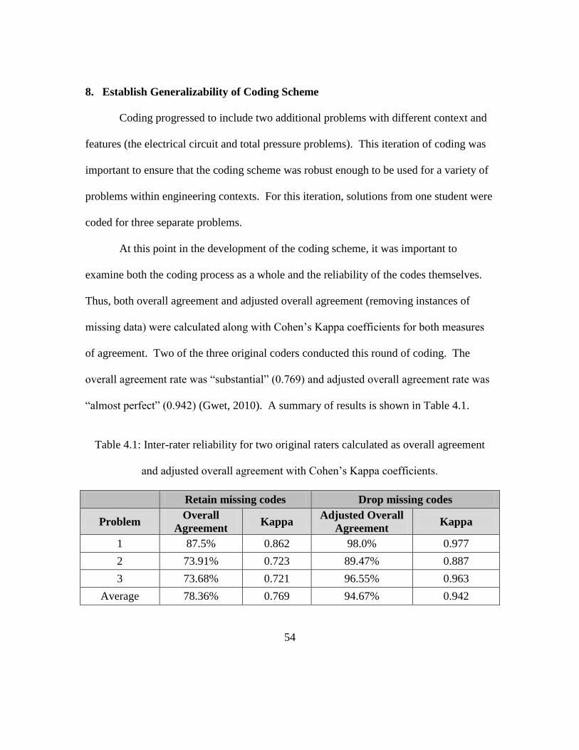
54

8. Establish Generalizability of Coding Scheme

Coding progressed to include two additional problems with different context and

features (the electrical circuit and total pressure problems). This iteration of coding was

important to ensure that the coding scheme was robust enough to be used for a variety of

problems within engineering contexts. For this iteration, solutions from one student were

coded for three separate problems.

At this point in the development of the coding scheme, it was important to

examine both the coding process as a whole and the reliability of the codes themselves.

Thus, both overall agreement and adjusted overall agreement (removing instances of

missing data) were calculated along with Cohen’s Kappa coefficients for both measures

of agreement. Two of the three original coders conducted this round of coding. The

overall agreement rate was “substantial” (0.769) and adjusted overall agreement rate was

“almost perfect” (0.942) (Gwet, 2010). A summary of results is shown in Table 4.1.

Table 4.1: Inter-rater reliability for two original raters calculated as overall agreement

and adjusted overall agreement with Cohen’s Kappa coefficients.

Retain missing codes Drop missing codes

Problem Overall

Agreement Kappa

Adjusted Overall

Agreement Kappa

1 87.5% 0.862 98.0% 0.977

2 73.91% 0.723 89.47% 0.887

3 73.68% 0.721 96.55% 0.963

Average 78.36% 0.769 94.67% 0.942

55

9. Assess Repeatability of Coding Scheme With New Rater

After a comprehensive coding scheme was developed, another member was

brought into the team to serve as an additional check that other researchers beside those

who developed the coding scheme can properly utilize the coding scheme. The new team

member was a post-doctoral researcher with a background in computer science education.

The new coder was trained in how to use the coding scheme by coding three solutions

openly with another coder, discussing questions encountered, and subsequently updating

the codebook. Once the new rater felt confident to progress, two of the initial raters

along with the new rater assessed one problem from each of the three problem sets

collected (the solar efficiency, electrical circuit, and total pressure problems) from one

student.

Inter-rater agreement showed that agreement was acceptable. Again, both overall

agreement and adjusted overall agreement (removing instances of missing data) were

calculated along with Cohen’s Kappa coefficients for both measures of agreement. As

shown in Table 4.2, inter-rater reliability decreased with the addition of the new coder,

but remained “substantial” for problems 1 and 2 and “almost perfect” when adjusted to

remove data points with missing ratings. In problem 3, there was a fairly sizeable portion

that was not coded because the student was iterating through the same element repeatedly

and these iterations were not captured by the new coder, resulting in only “fair”

agreement. For the efficiency problem from which the coding scheme was initially

developed, the agreement rates were 70% (98% adjusted). The agreement rate was 62%

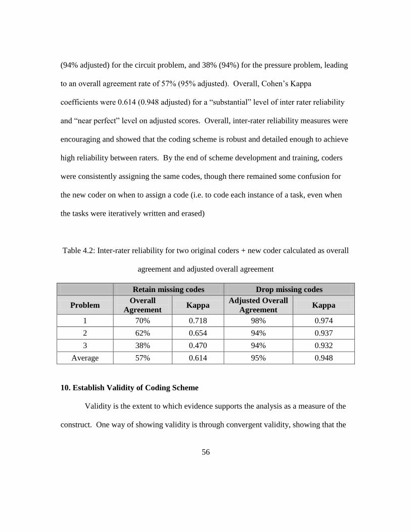
56

(94% adjusted) for the circuit problem, and 38% (94%) for the pressure problem, leading

to an overall agreement rate of 57% (95% adjusted). Overall, Cohen’s Kappa

coefficients were 0.614 (0.948 adjusted) for a “substantial” level of inter rater reliability

and “near perfect” level on adjusted scores. Overall, inter-rater reliability measures were

encouraging and showed that the coding scheme is robust and detailed enough to achieve

high reliability between raters. By the end of scheme development and training, coders

were consistently assigning the same codes, though there remained some confusion for

the new coder on when to assign a code (i.e. to code each instance of a task, even when

the tasks were iteratively written and erased)

Table 4.2: Inter-rater reliability for two original coders + new coder calculated as overall

agreement and adjusted overall agreement

Retain missing codes Drop missing codes

Problem Overall

Agreement Kappa

Adjusted Overall

Agreement Kappa

1 70% 0.718 98% 0.974

2 62% 0.654 94% 0.937

3 38% 0.470 94% 0.932

Average 57% 0.614 95% 0.948

10. Establish Validity of Coding Scheme

Validity is the extent to which evidence supports the analysis as a measure of the

construct. One way of showing validity is through convergent validity, showing that the

57

new assessment relates to other constructs it is supposed to relate to (Gatignon, 2009).

We compared data from the analysis of the first problem (the solar efficiency problem) to

ensure that the results obtained are in line with those obtained by others when examining

problem solving with respect to expertise (Chi, et al., 1981). Tables 4.3 and 4.4

summarize the data used to make this comparison.

Solutions were divided into four groups based on their approach strategy (as a

proxy of expertise level as evidenced in this particular solution). By stepping through the

problem solving process, one can get a sense for the level of expertise of the problem

solver through the strategies used based on how efficiently the problem solver moves

toward the goal or synthesizes information. In order from lowest to highest level of

elegance, the common strategies identified in this analysis included:

1) Plug and chug which involves inserting given values into an equation and

producing an answer without necessarily understanding the problem (Wankat,

1999).

2) Guess and Check which is a slightly more sophisticated approach where the

problem solver checks that the values inserted into an equation yields the

correct units or checks for reasonableness of the solution (Wankat, 1999).

3) Problem Decomposition (segmentation) which involves breaking down a

complex problem to ease analysis (Nickerson, 1994).

4) Clustering (chunking) which involves grouping like information into larger

units (Chi, et al., 1981)

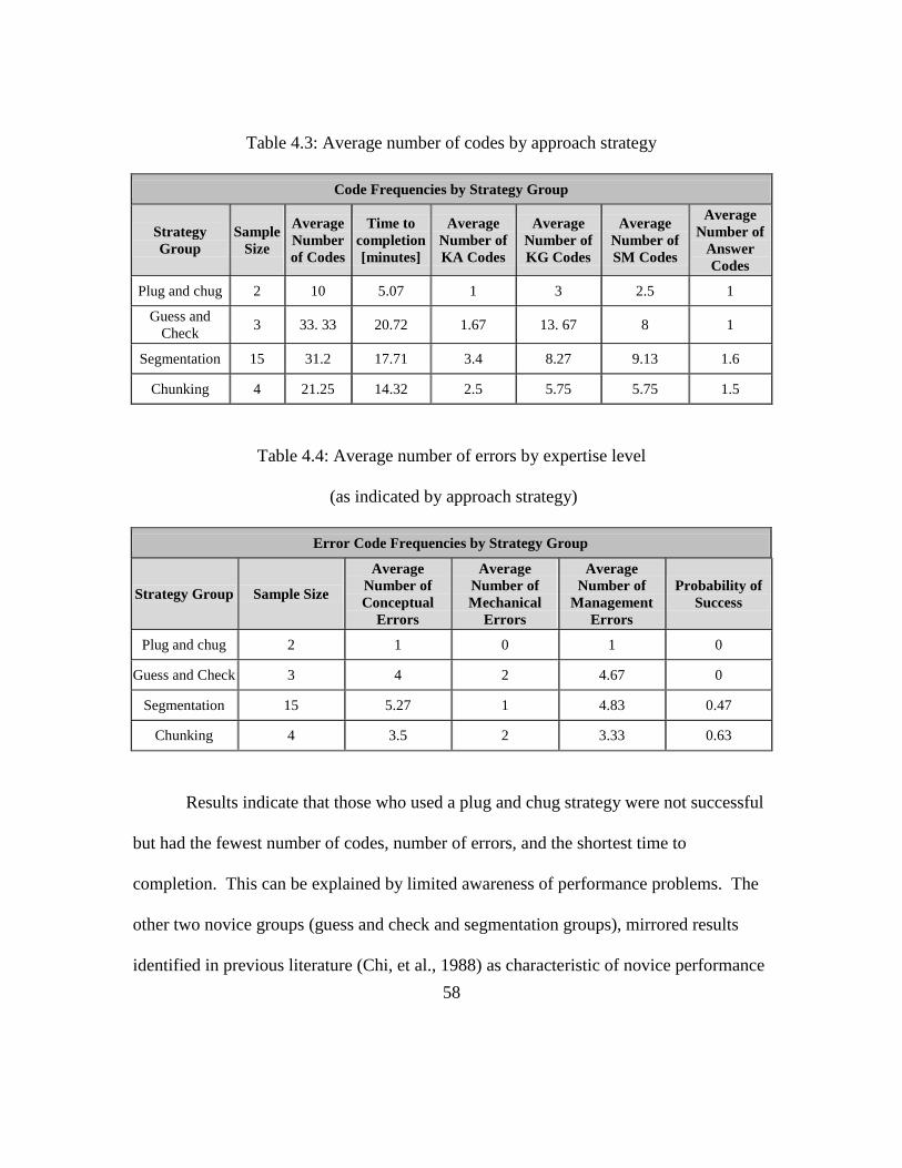
58

Table 4.3: Average number of codes by approach strategy

Code Frequencies by Strategy Group

Strategy

Group

Sample

Size

Average

Number

of Codes

Time to

completion

[minutes]

Average

Number of

KA Codes

Average

Number of

KG Codes

Average

Number of

SM Codes

Average

Number of

Answer

Codes

Plug and chug 2 10 5.07 1 3 2.5 1

Guess and

Check 3 33. 33 20.72 1.67 13. 67 8 1

Segmentation 15 31.2 17.71 3.4 8.27 9.13 1.6

Chunking 4 21.25 14.32 2.5 5.75 5.75 1.5

Table 4.4: Average number of errors by expertise level

(as indicated by approach strategy)

Error Code Frequencies by Strategy Group

Strategy Group Sample Size

Average

Number of

Conceptual

Errors

Average

Number of

Mechanical

Errors

Average

Number of

Management

Errors

Probability of

Success

Plug and chug 2 1 0 1 0

Guess and Check 3 4 2 4.67 0

Segmentation 15 5.27 1 4.83 0.47

Chunking 4 3.5 2 3.33 0.63

Results indicate that those who used a plug and chug strategy were not successful

but had the fewest number of codes, number of errors, and the shortest time to

completion. This can be explained by limited awareness of performance problems. The

other two novice groups (guess and check and segmentation groups), mirrored results

identified in previous literature (Chi, et al., 1988) as characteristic of novice performance

59

including longer time to completions, more errors, and a lower probability of success

than the more expert level of performance (chunking group). Our results indicated faster

completion time for more expert performance, though the results showed a more

moderate difference between them and the more novice performance groups than what

was observed in the research by Chi et al., namely four times faster. (Average

completion times for “novice” groups, guess and check and segmentation, were 20.72

minutes and 17.71 minutes, respectively, compared to the “expert” performance group,

chunking, which was14.32 minutes). Our research supports the claim that novices

commit more errors; guess and check and segmentation groups committed an average of

10.67 and 11.1 errors respectively, compared to the chunking group, with an average of

8.83 errors. This indicates that this coding scheme provides a reasonable assessment of

problem solving performance as indicated by relative expertise of the students.

CONCLUSION

This paper describes the methodology used to develop a robust coding scheme for

the analysis of problem solving skills in a first year engineering program. Using this

coding scheme, solutions were analyzed based on actions taken as a result of cognitive

and metacognitive processes, which are categorized as knowledge access, knowledge

generation, self-management, as well as errors (categorized as conceptual, mechanical,

and management errors), approach strategies and solution accuracy. For our research, a

60

mixed model methodology is used in order to assess problem solving skills levels by first

quantitizing the data from students’ written problem solutions. While the coding scheme

was developed and validated using a set of well-defined story problems typical of a first

year engineering course, because of the general nature of the categories of processes,

errors, and strategies, it may be transferrable to other types of engineering problems that

are more ill-defined or complex in nature.

Other researchers can use this methodology in their coding scheme development

efforts for analyzing qualitative data related to complex processes. By following the

procedure, we were able to ensure reliable coding among coders from different

backgrounds and perspectives. However, it takes significant effort to train coders, and

researchers should be leery about bringing in new coders unless there is a formal training

and an assessment process to ensure consistency in coding. Ultimately, we chose to have

one coder code all remaining solutions and the other coder review those coded solutions

to ensure accuracy. While this step effectively doubled the time needed to the code data,

the step was important for ensuring quality, even though relatively few edits were

suggested by the reviewer following the training process.

This coding scheme is being used to assess problem solutions of first year

engineering students at a large southeastern university. The process element, error, and

strategy codes enable the assessment of various problem solving skills necessary to

progress through the problem solving cycle. When the output of coded solutions is

loaded into a database, the data can be queried in a number of ways to transform

61

individual codes into meaningful measures of performance. That information can then be

used to give insight to researchers and ultimately instructors and students. Using this

information, the relationships between problem solving skills and students’ academic

preparation are being evaluated for its relationships to problem solving success and

mental workload.

62

CHAPTER FIVE:

ESTABLISHING MEASURES OF PROBLEM SOLVING PERFORMANCE

As problem solving is an important skill for engineers to master, engineering

educators should strive to help students obtain the knowledge and skills required for

problem solving success. However, in order to assess the development of skills, it is

necessary to be able to assess students’ individual performances on a common set of

criteria at various points in their studies. The purpose of this chapter is to establish a

standardized method for assessing problem solutions in terms of performance based on

activities involved in the problem solving process. The resulting list of performance

measures will be used to evaluate student performance in a first year engineering course.

In total, 28 internal process measures and 12 outcome measures were established.

INTRODUCTION

Performance assessment, the direct systematic appraisal of performance compared

to a pre-determined set of criteria, have been shown to improve students’ mathematical

problem solving (Fuchs, Fuchs, Karns, Hamlett, & Katzaroff, 1999). Effective

performance assessment requires that metrics be developed in order to compare processes

of complementary entities (Damelio, 1995). While some instructors and even school

systems have utilized performance assessments to measure students’ problem solving

63

competency, it is still not common practice. An initiative aimed at helping teachers

develop performance assessments found that “time is a major obstacle to changing

classroom practice” (Borko, Mayfield, Marion, Flexer, & Cumbo, 1997).

Research by Slater emphasizes the importance of performance assessment of

problem solving skills, especially for STEM (science, technology, engineering, and

mathematics) majors because it provides insight to a student’s level of conceptual and

procedural knowledge (Slater, 1993). Slater states that the purpose of conducting

performance assessments is “to evaluate the actual process of doing science or

mathematics” (Slater, 1993, p. 3). It can be used for a variety of purposes including: 1)

diagnostic purposes to determine what students know, 2) instructional purposes such as in

class activities, or 3) monitoring purposes as through multiple iterations of evaluation to

evaluate changes in skills. While Slater suggests performance assessment should be

conducted with live evaluations of ill-defined tasks, there is no reason that performance

assessment must be limited to this type of activity, where only one person or group can

be evaluated at a time. His recommendation is in part due to the weaknesses of

conventional paper and pencil assessments. However, by overcoming this barrier with

technology that captures the entire problem solving process instead of a snapshot of the

final solution (Bowman & Benson, 2010; Grigg & Benson, 2011), performance

assessment can be applied to traditional learning activities for a larger population of

students through evaluating archived data rather than live demonstrations.

64

ESTABLISHING MEASURES OF PROBLEM SOLVING PERFORMANCE

The remainder of this chapter details how the elements from the coding scheme,

shown in Appendix D, were used to establish objective measures of performance

throughout the problem solving processes. Using a mixed model methodology, problem

solving performance was evaluated by quantitizing coded data from students’ written

problem solutions (Tashakkori & Teddlie, 1998). Problem solving was assessed along a

seven stage cycle consisting of: 1) recognize / identify the problem, 2) define and

represent the problem, 3) develop a solution strategy, 4) organize knowledge about the

problem, 5) allocate resources for solving the problem, 6) monitor progress toward the

goals, and 7) evaluate the solution (Pretz, et al., 2003).

However, in practice, there is much variability in how people approach the

problem solving process. The proposed stages are not utilized by all problem solvers in

all situations, and the problem solver may iterate between one or more stages as s/he

responds to feedback (either internal or external) on progression toward solving the

problem (Wilson, et al., 1993). Rather than viewing these stages as independent, it is

more representative to think of them as concurrent subprocesses where actions taken in

one subprocess may prompt action in another (Samsonowa, 2011, p. 27). This approach

differs from models that evaluate problem solving as independent phases, such the

Integrated Problem Solving (IPS) model, which can imply that students do not revise

their initial understanding of the problem (phase 1) if the revisions occur after the student

65

draws a picture, i.e. entered the second phase (Litzinger, et al., 2010).

In order to formulate performance measures for these problem solving processes,

a variety of sources were investigated on measures of similar skills from the education

and human performance literature. Measures were broken down into two forms:

1) internal process measures and 2) outcome measures. Internal process measures look at

how thoroughly, accurately, and efficiently tasks are completed. Outcome measures

evaluate whether the process is producing the desired results. By comparing internal

process measures to outcome measures, one can determine which factors contribute to the

desired results (Harmon, 2008).

MEASURES OF PROBLEM SOLVING PROCESSES

Education and human performance literature was utilized in determining

measures that adequately evaluate student performance within the seven stages of

Sternberg’s problem solving cycle. Twenty-eight internal process measures were created

and used to evaluate student problem solving attempts. Table 5.1 describes the breakout

of the number of measures across stages. A complete list of developed metrics along

with their calculation and measure type can be seen in Appendix E.

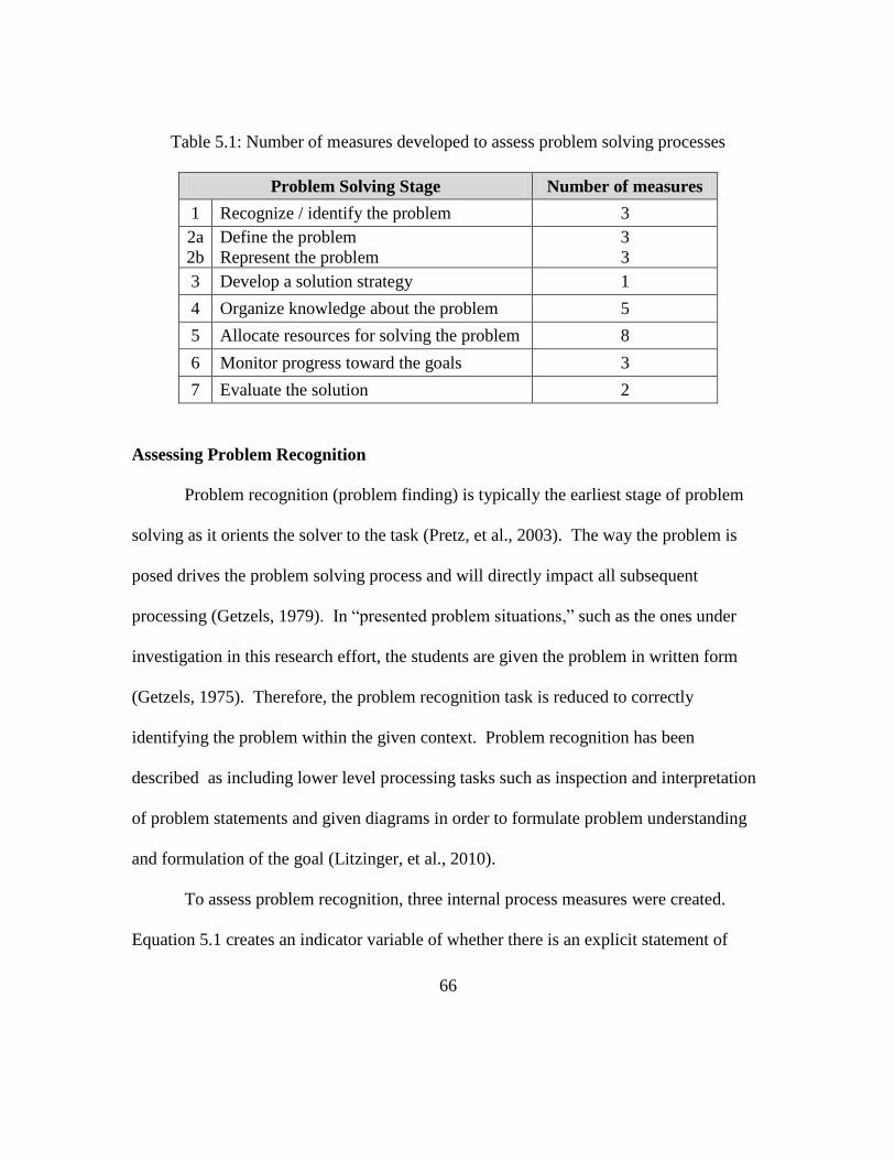
66

Table 5.1: Number of measures developed to assess problem solving processes

Problem Solving Stage Number of measures

1 Recognize / identify the problem 3

2a

2b

Define the problem

Represent the problem

3

3

3 Develop a solution strategy 1

4 Organize knowledge about the problem 5

5 Allocate resources for solving the problem 8

6 Monitor progress toward the goals 3

7 Evaluate the solution 2

Assessing Problem Recognition

Problem recognition (problem finding) is typically the earliest stage of problem

solving as it orients the solver to the task (Pretz, et al., 2003). The way the problem is

posed drives the problem solving process and will directly impact all subsequent

processing (Getzels, 1979). In “presented problem situations,” such as the ones under

investigation in this research effort, the students are given the problem in written form

(Getzels, 1975). Therefore, the problem recognition task is reduced to correctly

identifying the problem within the given context. Problem recognition has been

described as including lower level processing tasks such as inspection and interpretation

of problem statements and given diagrams in order to formulate problem understanding

and formulation of the goal (Litzinger, et al., 2010).

To assess problem recognition, three internal process measures were created.

Equation 5.1 creates an indicator variable of whether there is an explicit statement of

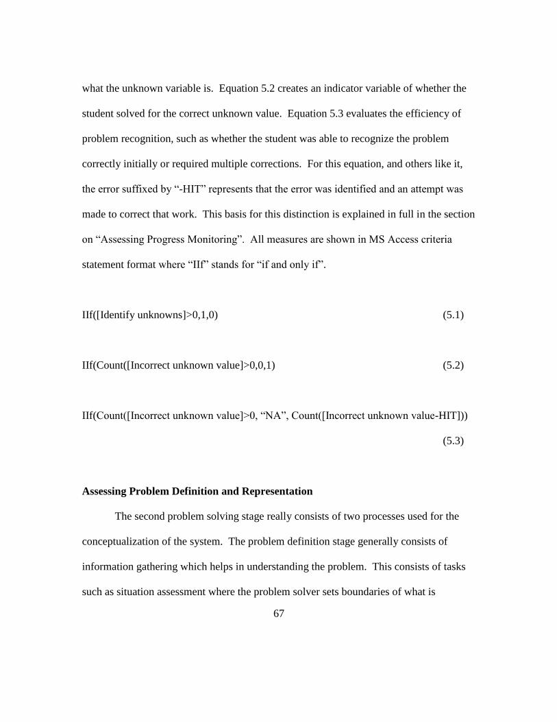
67

what the unknown variable is. Equation 5.2 creates an indicator variable of whether the

student solved for the correct unknown value. Equation 5.3 evaluates the efficiency of

problem recognition, such as whether the student was able to recognize the problem

correctly initially or required multiple corrections. For this equation, and others like it,

the error suffixed by “-HIT” represents that the error was identified and an attempt was

made to correct that work. This basis for this distinction is explained in full in the section

on “Assessing Progress Monitoring”. All measures are shown in MS Access criteria

statement format where “IIf” stands for “if and only if”.

IIf([Identify unknowns]>0,1,0) (5.1)

IIf(Count([Incorrect unknown value]>0,0,1) (5.2)

IIf(Count([Incorrect unknown value]>0, “NA”, Count([Incorrect unknown value-HIT]))

(5.3)

Assessing Problem Definition and Representation

The second problem solving stage really consists of two processes used for the

conceptualization of the system. The problem definition stage generally consists of

information gathering which helps in understanding the problem. This consists of tasks

such as situation assessment where the problem solver sets boundaries of what is

68

included or excluded and interprets the situation (Smith, 1998). This stage might include

tasks such as restating the problem, identifying assumptions, or identifying constraints.

To assess problem definition, three internal process measures were created.

Equation 5.4 creates a count of the number of explicit problem definition statements.

Equation 5.5 creates an indicator variable of whether the student correctly defined the

problem. Equation 5.6 evaluates the efficiency of problem definition, such as whether

the problem was correctly defined initially or required correction.

Sum(IIf(Count([Restate problem]>0,1,0)) + IIf(Count([Identify assumption]>0,1,0))+

IIf(Count([Identify constraint]>0,1,0))) (5.4)

IIf(Count([Ignored problem constraint]>0,0,IIf(Count([Incorrect assumption]>0,0,1) )

(5.5)

IIf(Count([Ignored problem constraint]>0, “NA”, IIf(Count([Incorrect assumption]>0,

“NA”, Sum(Count([Ignored problem constraint -HIT])+ Count([Incorrect

assumption -HIT]))) (5.6)

Problem representation is recognized as an important step in the problem solving

process (Jonassen, et al., 2006). A study of mathematical problem solving showed a

positive correlation with schematic spatial representations, but a negative correlation with

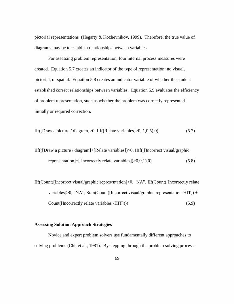
69

pictorial representations (Hegarty & Kozhevnikov, 1999). Therefore, the true value of

diagrams may be to establish relationships between variables.

For assessing problem representation, four internal process measures were

created. Equation 5.7 creates an indicator of the type of representation: no visual,

pictorial, or spatial. Equation 5.8 creates an indicator variable of whether the student

established correct relationships between variables. Equation 5.9 evaluates the efficiency

of problem representation, such as whether the problem was correctly represented

initially or required correction.

IIf([Draw a picture / diagram]>0, IIf([Relate variables]>0, 1,0.5),0) (5.7)

IIf(([Draw a picture / diagram]+[Relate variables])>0, IIIf(([Incorrect visual/graphic

representation]+[ Incorrectly relate variables])>0,0,1),0) (5.8)

IIf(Count([Incorrect visual/graphic representation]>0, “NA”, IIf(Count([Incorrectly relate

variables]>0, “NA”, Sum(Count([Incorrect visual/graphic representation-HIT]) +

Count([Incorrectly relate variables -HIT]))) (5.9)

Assessing Solution Approach Strategies

Novice and expert problem solvers use fundamentally different approaches to

solving problems (Chi, et al., 1981). By stepping through the problem solving process,

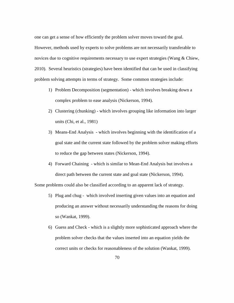
70

one can get a sense of how efficiently the problem solver moves toward the goal.

However, methods used by experts to solve problems are not necessarily transferable to

novices due to cognitive requirements necessary to use expert strategies (Wang & Chiew,

2010). Several heuristics (strategies) have been identified that can be used in classifying

problem solving attempts in terms of strategy. Some common strategies include:

1) Problem Decomposition (segmentation) - which involves breaking down a

complex problem to ease analysis (Nickerson, 1994).

2) Clustering (chunking) - which involves grouping like information into larger

units (Chi, et al., 1981)

3) Means-End Analysis - which involves beginning with the identification of a

goal state and the current state followed by the problem solver making efforts

to reduce the gap between states (Nickerson, 1994).

4) Forward Chaining - which is similar to Mean-End Analysis but involves a

direct path between the current state and goal state (Nickerson, 1994).

Some problems could also be classified according to an apparent lack of strategy.

5) Plug and chug - which involved inserting given values into an equation and

producing an answer without necessarily understanding the reasons for doing

so (Wankat, 1999).

6) Guess and Check - which is a slightly more sophisticated approach where the

problem solver checks that the values inserted into an equation yields the

correct units or checks for reasonableness of the solution (Wankat, 1999).

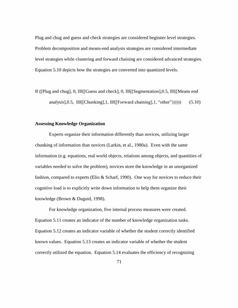
71

Plug and chug and guess and check strategies are considered beginner level strategies.

Problem decomposition and means-end analysis strategies are considered intermediate

level strategies while clustering and forward chaining are considered advanced strategies.

Equation 5.10 depicts how the strategies are converted into quantized levels.

If ([Plug and chug], 0, IIf([Guess and check], 0, IIf([Segmentation],0.5, IIf([Means end

analysis],0.5, IIf([Chunking],1, IIf([Forward chaining],1, “other”)))))) (5.10)

Assessing Knowledge Organization

Experts organize their information differently than novices, utilizing larger

chunking of information than novices (Larkin, et al., 1980a). Even with the same

information (e.g. equations, real world objects, relations among objects, and quantities of

variables needed to solve the problem), novices store the knowledge in an unorganized

fashion, compared to experts (Elio & Scharf, 1990). One way for novices to reduce their

cognitive load is to explicitly write down information to help them organize their

knowledge (Brown & Duguid, 1998).

For knowledge organization, five internal process measures were created.

Equation 5.11 creates an indicator of the number of knowledge organization tasks.

Equation 5.12 creates an indicator variable of whether the student correctly identified

known values. Equation 5.13 creates an indicator variable of whether the student

correctly utilized the equation. Equation 5.14 evaluates the efficiency of recognizing

72

known information while equation 5.15 evaluates the efficiency of recognizing equations,

specifically whether this information was correctly identified initially or required

correction.

Sum(IIf(Count([Identify known values]>0,1,0)) + IIf(Count([Identify equation]>0,1,0)))

(5.11)

IIf(Count([Incorrect known value]>0,0,1) (5.12)

IIf(Count([Misuse governing equation]>0,0,1) (5.13)

IIf(Count([Incorrect known value]>0, “NA”, Count([Incorrect known value-HIT]))

(5.14)

IIf(Count([Misuse equation]>0, “NA”, Count([Misuse equation -HIT])) (5.15)

Assessing How Resources are Allocated for Execution (Knowledge Generation)

During the problem solving process, it is important to manage cognitive resources

effectively. However, people often rely on intuition in order to reduce the level of effort

or use ineffective methods that increase cognitive effort. Striking a proper balance is

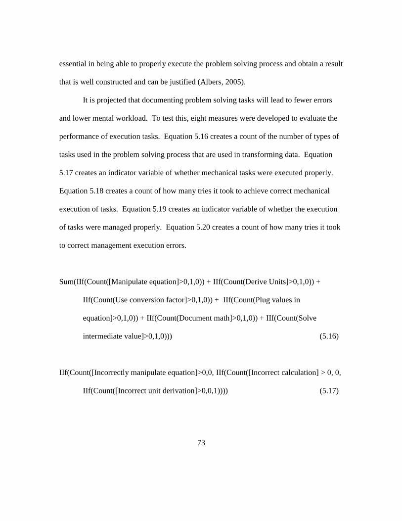
73

essential in being able to properly execute the problem solving process and obtain a result

that is well constructed and can be justified (Albers, 2005).

It is projected that documenting problem solving tasks will lead to fewer errors

and lower mental workload. To test this, eight measures were developed to evaluate the

performance of execution tasks. Equation 5.16 creates a count of the number of types of

tasks used in the problem solving process that are used in transforming data. Equation

5.17 creates an indicator variable of whether mechanical tasks were executed properly.

Equation 5.18 creates a count of how many tries it took to achieve correct mechanical

execution of tasks. Equation 5.19 creates an indicator variable of whether the execution

of tasks were managed properly. Equation 5.20 creates a count of how many tries it took

to correct management execution errors.

Sum(IIf(Count([Manipulate equation]>0,1,0)) + IIf(Count(Derive Units]>0,1,0)) +

IIf(Count(Use conversion factor]>0,1,0)) + IIf(Count(Plug values in

equation]>0,1,0)) + IIf(Count(Document math]>0,1,0)) + IIf(Count(Solve

intermediate value]>0,1,0))) (5.16)

IIf(Count([Incorrectly manipulate equation]>0,0, IIf(Count([Incorrect calculation] > 0, 0,

IIf(Count([Incorrect unit derivation]>0,0,1)))) (5.17)

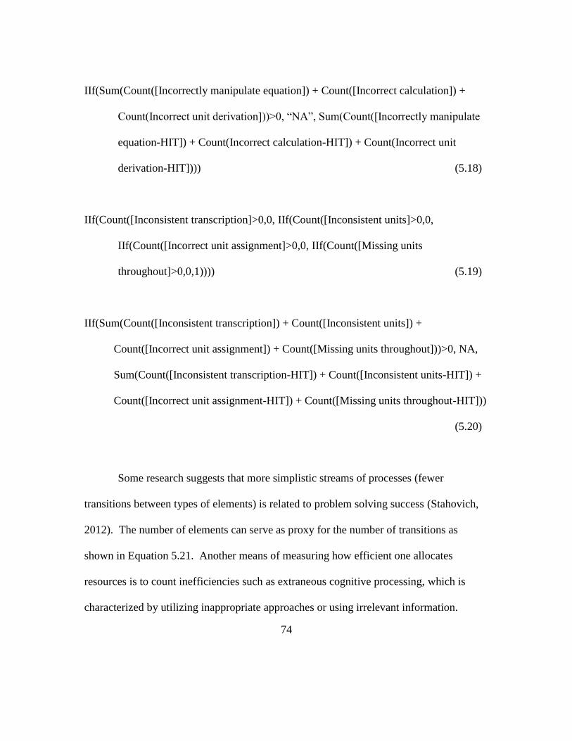
74

IIf(Sum(Count([Incorrectly manipulate equation]) + Count([Incorrect calculation]) +

Count(Incorrect unit derivation]))>0, “NA”, Sum(Count([Incorrectly manipulate

equation-HIT]) + Count(Incorrect calculation-HIT]) + Count(Incorrect unit

derivation-HIT]))) (5.18)

IIf(Count([Inconsistent transcription]>0,0, IIf(Count([Inconsistent units]>0,0,

IIf(Count([Incorrect unit assignment]>0,0, IIf(Count([Missing units

throughout]>0,0,1)))) (5.19)

IIf(Sum(Count([Inconsistent transcription]) + Count([Inconsistent units]) +

Count([Incorrect unit assignment]) + Count([Missing units throughout]))>0, NA,

Sum(Count([Inconsistent transcription-HIT]) + Count([Inconsistent units-HIT]) +

Count([Incorrect unit assignment-HIT]) + Count([Missing units throughout-HIT]))

(5.20)

Some research suggests that more simplistic streams of processes (fewer

transitions between types of elements) is related to problem solving success (Stahovich,

2012). The number of elements can serve as proxy for the number of transitions as

shown in Equation 5.21. Another means of measuring how efficient one allocates

resources is to count inefficiencies such as extraneous cognitive processing, which is

characterized by utilizing inappropriate approaches or using irrelevant information.

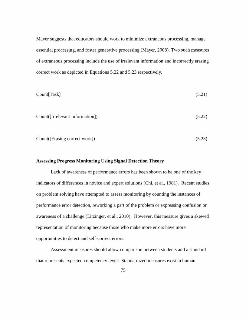
75

Mayer suggests that educators should work to minimize extraneous processing, manage

essential processing, and foster generative processing (Mayer, 2008). Two such measures

of extraneous processing include the use of irrelevant information and incorrectly erasing

correct work as depicted in Equations 5.22 and 5.23 respectively.

Count[Task] (5.21)

Count([Irrelevant Information]) (5.22)

Count([Erasing correct work]) (5.23)

Assessing Progress Monitoring Using Signal Detection Theory

Lack of awareness of performance errors has been shown to be one of the key

indicators of differences in novice and expert solutions (Chi, et al., 1981). Recent studies

on problem solving have attempted to assess monitoring by counting the instances of

performance error detection, reworking a part of the problem or expressing confusion or

awareness of a challenge (Litzinger, et al., 2010). However, this measure gives a skewed

representation of monitoring because those who make more errors have more

opportunities to detect and self-correct errors.

Assessment measures should allow comparison between students and a standard

that represents expected competency level. Standardized measures exist in human

76

performance literature that provide scores that are adjusted to account for process

variations such as different number of errors. Using Signal Detection Theory, error

detection can be measured, as a proxy for monitoring, in a way that enables comparison

between solutions either across people or across assignments. Signal Detection Theory,

was first described by Green and Swets to evaluate a decision maker’s performance

detecting a signal when there was unpredictable variability present (Green & Swets,

1966). Since then, the theory has been utilized in a range of contexts including

measuring the ability to recognize stimuli such as tumors in medical diagnostics or

weapons in air travel luggage scans (Macmillan & Creelman, 2005). Recent work in

education has used Detection Theory to analyze rater behavior in essay grading and

assessment of student abilities (Abdi, 2009). Detection Theory quantifies the reaction of

an observer to the presentation of a signal in an environment containing noise as one of

four classifications based on whether the stimuli was present or not and whether the

observer responded as if the stimuli was present or not.

Measuring error detection in student work can be done by classifying problem

solving activities as one of four states: 1) HIT is when there is an error and the student

recognized an error, 2) MISS is when there is an error and the student does not recognize

the error, 3) FALSE ALARM is when there is not an error but the student identified it as

having an error, and 4) CORRECT REJECTION is when there is no error and the student

correctly does not recognize an error. Table 5.2 illustrates the error monitoring states

given error present and error absent conditions.

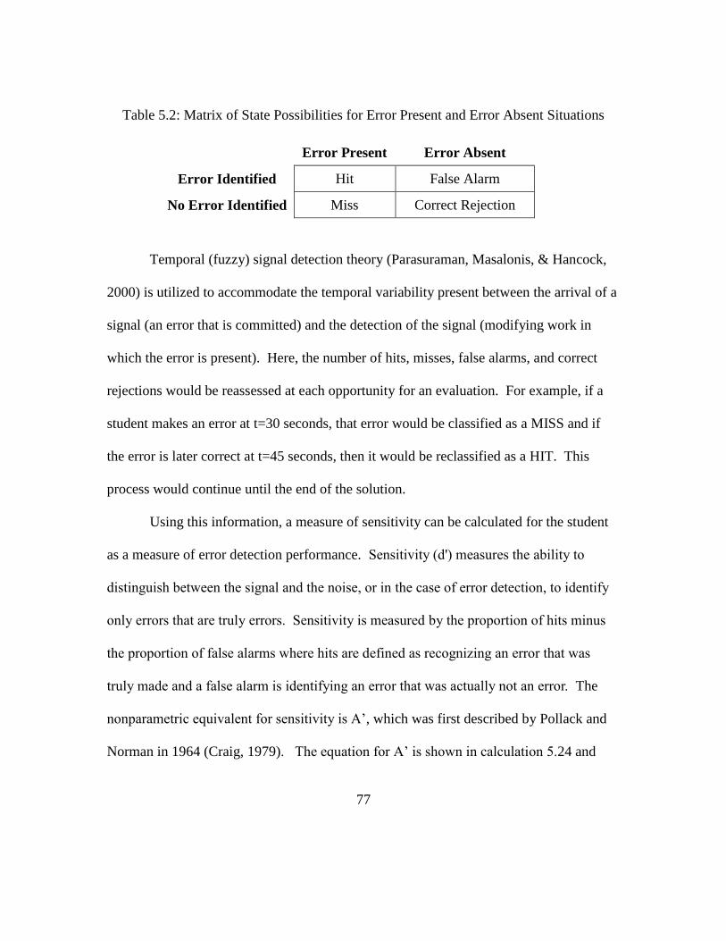
77

Table 5.2: Matrix of State Possibilities for Error Present and Error Absent Situations

Error Present Error Absent

Error Identified Hit False Alarm

No Error Identified Miss Correct Rejection

Temporal (fuzzy) signal detection theory (Parasuraman, Masalonis, & Hancock,

2000) is utilized to accommodate the temporal variability present between the arrival of a

signal (an error that is committed) and the detection of the signal (modifying work in

which the error is present). Here, the number of hits, misses, false alarms, and correct

rejections would be reassessed at each opportunity for an evaluation. For example, if a

student makes an error at t=30 seconds, that error would be classified as a MISS and if

the error is later correct at t=45 seconds, then it would be reclassified as a HIT. This

process would continue until the end of the solution.

Using this information, a measure of sensitivity can be calculated for the student

as a measure of error detection performance. Sensitivity (d') measures the ability to

distinguish between the signal and the noise, or in the case of error detection, to identify

only errors that are truly errors. Sensitivity is measured by the proportion of hits minus

the proportion of false alarms where hits are defined as recognizing an error that was

truly made and a false alarm is identifying an error that was actually not an error. The

nonparametric equivalent for sensitivity is A’, which was first described by Pollack and

Norman in 1964 (Craig, 1979). The equation for A’ is shown in calculation 5.24 and

78

equations 5.25 and 5.26 show how to calculate the false alarm rate and hit rate needed to

assess sensitivity. The measure yields a value between 0 and 1 with scores similar to the

typical grading scale with 1.0 indicating perfect detection, 0.7 indicating fair detection,

0.5 indicates no discrimination, and values below 0.5 typically indicate an error of some

kind either confusion on the task or miscalculation by the researcher.

(5.24)

(5.25)

(5.26)

Assessing Solution Evaluation

The final problem solving step is to check the accuracy of the final answer. No matter

what the level of expertise, mistakes can be made, and it is important to check that the answer is

reasonable through techniques such as estimating what the answer should be or reworking

calculations. To assess a student checking accuracy, two internal process measures were

created. Equation 5.27 creates an indicator variable of whether there is explicit work that

documents checking work, such as rework following solution, an estimation, or other

#( )

# #

HITP H

HIT MISS

# _( )

# _ # _

FALSE ALARMP FA

FALSE ALARM CORRECT REJECTIONS

1 ( ) 1 ( )' 1

4 ( ) 1 ( )

P FA P HA

P H P FA

79

similar task. Equation 5.28 creates an indicator variable of whether there is an explicit

indication of what the final answer is. While not an explicit check for accuracy, it is a

verification that the final answer was reached.

IIf([Check accuracy]>0,1,0) (5.27)

IIf([Identify final answer]>0,1,0) (5.28)

MEASURES OF PERFORMANCE OUTCOMES

Traditionally, instructors evaluate students’ solutions based on the accuracy of the

final answer. Sometimes other considerations come into account such as whether the

student indicates confidence in their answer (Szetela, 1987). However, other measures

can be used to evaluate the solution in terms of process efficiency and student stress

levels following completion of the task. Twelve outcome measures were created and

used to evaluate the resulting outcomes of student problem solving attempts. Table 5.3

describes the breakout of the number of measures across each entity (Jablokow, 2007). A

complete list of developed metrics along with their calculation and measure type can be

seen in Appendix F.

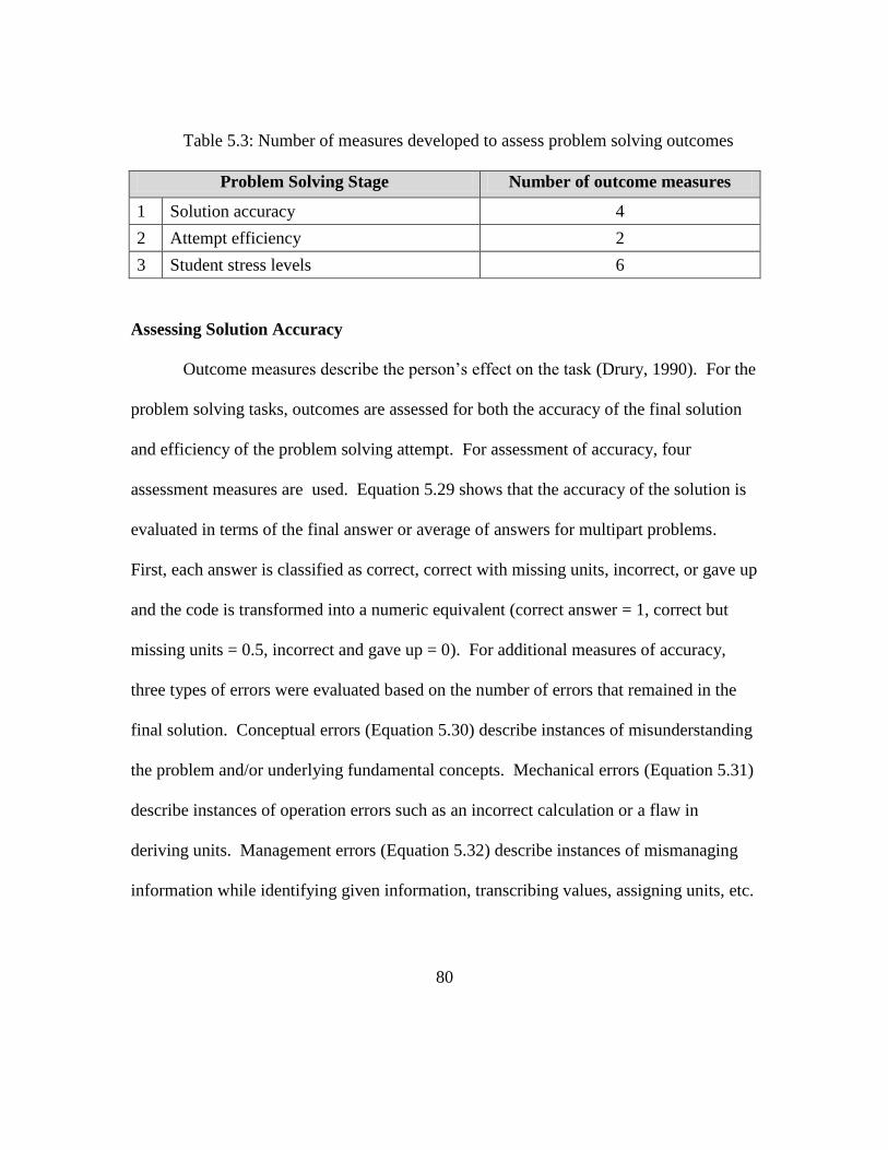
80

Table 5.3: Number of measures developed to assess problem solving outcomes

Problem Solving Stage Number of outcome measures

1 Solution accuracy 4

2 Attempt efficiency 2

3 Student stress levels 6

Assessing Solution Accuracy

Outcome measures describe the person’s effect on the task (Drury, 1990). For the

problem solving tasks, outcomes are assessed for both the accuracy of the final solution

and efficiency of the problem solving attempt. For assessment of accuracy, four

assessment measures are used. Equation 5.29 shows that the accuracy of the solution is

evaluated in terms of the final answer or average of answers for multipart problems.

First, each answer is classified as correct, correct with missing units, incorrect, or gave up

and the code is transformed into a numeric equivalent (correct answer = 1, correct but

missing units = 0.5, incorrect and gave up = 0). For additional measures of accuracy,

three types of errors were evaluated based on the number of errors that remained in the

final solution. Conceptual errors (Equation 5.30) describe instances of misunderstanding

the problem and/or underlying fundamental concepts. Mechanical errors (Equation 5.31)

describe instances of operation errors such as an incorrect calculation or a flaw in

deriving units. Management errors (Equation 5.32) describe instances of mismanaging

information while identifying given information, transcribing values, assigning units, etc.

81

Average [Answer State] (5.29)

Count[Conceptual Errors (not corrected)] (5.30)

Count[Mechanical Errors (not corrected)] (5.31)

Count[Management Errors (not corrected)] (5.32)

Assessing Attempt Efficiency

For assessing of the problem solving attempt, two measures were created based

on human performance literature. The error rate serves as a measure of human reliability

by indicating the frequency of occurrence of quality problems (Equation 5.33).

The time to completion, equation 5.34 is a performance measure traditionally used to

assess human performance, as often accuracy is compromised in favor of speed (Drury,

1990).

Count Errors

Count Tasks

(5.32)

[End time]-[Start time] (5.33)

82

Assessing Stress Measures

The final outcome measure is the impact of the task on the student. This is

measured in terms of the students’ mental workload. If cognitive resources are adequate

during the completion of the task, mental workload would be lower than if resources

were inadequate. While there are several methods for assessing mental workload, one of

the best methods in terms of ease of data collection and analysis is using a standard self-

report measure such as the NASA-TLX (Hart, 2006). The NASA-TLX consists of six

subscales, three measuring demand put on the participant by the task and three measuring

stress added by the worker because of interacting with the task. The three measures of

task demand include 1) mental demand, 2) physical demand, and 3) temporal demand.

The remaining measures, 4) effort, 5) performance, and 6) frustration, describe the stress

put on the person by the interaction of the person with the task (Warm, et al., 2008);

however, physical demand is irrelevant for cognitive tasks and can be excluded from

analysis. The NASA-TLX subscales are scored on a continuous scale from zero to

twenty (Stanton, et al., 2005). Using this scale, a measure of workload can be calculated

by summing the values from individual subscores as shown in Equation 5.35. However,

the individual subscale scores can also be used as indicators of specific stressors.

Sum([Mental Demand]+[Temporal Demand]+[Performance]+[Effort]+[Frustration])

(5.35)

83

These measures will serve as a means of comparing problem solving performance

in subsequent investigations. In Chapter 6, internal process measures are used in the

comparison of correct and incorrect solutions. In Chapter 7, internal process measures

are used in the comparison of outcome measures of mental workload. In Chapter 8,

internal process measures and outcome measures are used in the comparison of

participant factors including, gender, ethnicity, and prior academic experience.

Relationships are explored further in Chapter 9, which offers final recommendations on

the usefulness of measures in providing feedback to students on their problem solving

performance.

84

CHAPTER SIX

WHAT PROBLEM SOLVING FEATURES ARE MORE PREVALENT

IN SUCCESSFUL SOLUTIONS?

This investigation looks at enhancing research-based practice in higher education

by exploring what problem solving features and student actions are related to successful

problem solving attempts. The primary goal of this investigation was to compare

successful and unsuccessful solutions in terms of cognitive and metacognitive processes,

errors, and strategies, to elucidate key findings that can be incorporated into performance

evaluations of student work. Data from two semesters were included in this analysis. In

the first semester (n=27), students solved problems using their method of choice;

however, in the second semester (n=36), another cohort of students were asked to use

planning and visualization activities. As a secondary goal, this study evaluates the

effectiveness of this pedagogical intervention on improving problem solving performance

in the classroom. Variation in success across semesters was used as a proxy measure of

the effectiveness of this instructional intervention.

Results indicated that implementing the problem solving structure had a positive

impact on problem solving success. Additionally, statistical analysis of solution data

revealed that correct solutions were more likely to contain instances of 1) explicit

planning activities such as identifying unknown values and conversion factors, 2) explicit

manipulation of variables when converting between units, and 3) evidence of a means-

85

ends-analysis approach to solving the problem. There were also significant effects on

problem solving success from using conversion factors, documenting math, and utilizing

a chunking strategy to approach the problem, all of which were associated with correct

solutions. Incorrect solutions were more likely to contain instances of 1) implicit

equation identification, 2) ignoring problem constraints, 3) identifying errors, and 4)

evidence of a plug-and-chug approach to solving the problem. There were also

significant effects on problem solving success from labeling/renaming, incorrectly

relating variables, and inconsistent units, which were associated with incorrect solutions.

Next, performance measures were assessed to determine their ability to

discriminate between actions associated with successful versus unsuccessful solutions.

Sixteen of the twenty-eight proposed performance measures of processes were able to

distinguish between successful and unsuccessful problem solving attempts. This

information gives insight into the effectiveness of different strategies that novice problem

solvers use to manage the problem solving process. The ultimate goal of this project is to

inform the development of problems and instructional pedagogies for introductory

engineering courses which capitalize on successful strategies.

INTRODUCTION

Learning does not occur as a passive action. For meaningful learning to occur,

one must make sense out of newly presented information and form connections with

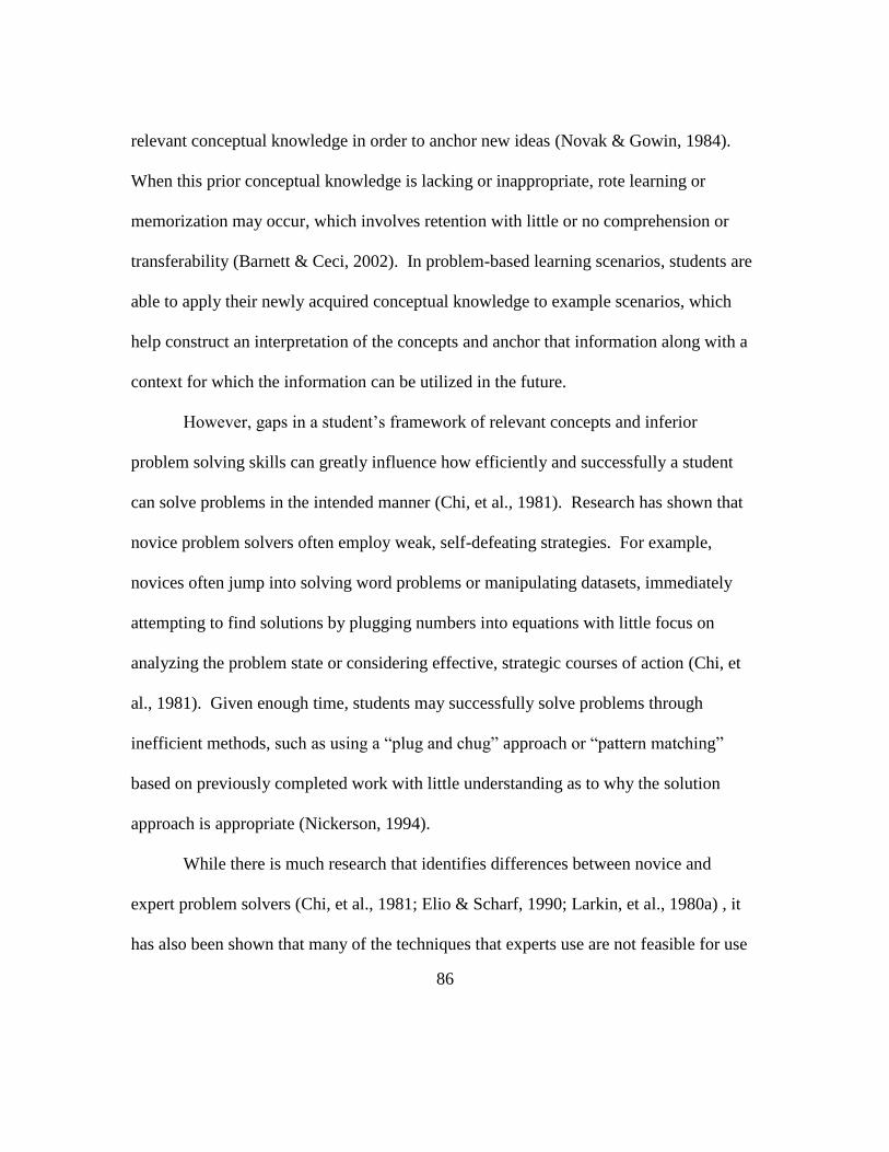
86

relevant conceptual knowledge in order to anchor new ideas (Novak & Gowin, 1984).

When this prior conceptual knowledge is lacking or inappropriate, rote learning or

memorization may occur, which involves retention with little or no comprehension or

transferability (Barnett & Ceci, 2002). In problem-based learning scenarios, students are

able to apply their newly acquired conceptual knowledge to example scenarios, which

help construct an interpretation of the concepts and anchor that information along with a

context for which the information can be utilized in the future.

However, gaps in a student’s framework of relevant concepts and inferior

problem solving skills can greatly influence how efficiently and successfully a student

can solve problems in the intended manner (Chi, et al., 1981). Research has shown that

novice problem solvers often employ weak, self-defeating strategies. For example,

novices often jump into solving word problems or manipulating datasets, immediately

attempting to find solutions by plugging numbers into equations with little focus on

analyzing the problem state or considering effective, strategic courses of action (Chi, et

al., 1981). Given enough time, students may successfully solve problems through

inefficient methods, such as using a “plug and chug” approach or “pattern matching”

based on previously completed work with little understanding as to why the solution

approach is appropriate (Nickerson, 1994).

While there is much research that identifies differences between novice and

expert problem solvers (Chi, et al., 1981; Elio & Scharf, 1990; Larkin, et al., 1980a) , it

has also been shown that many of the techniques that experts use are not feasible for use

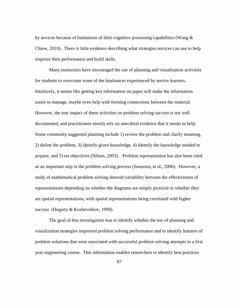
87

by novices because of limitations of their cognitive processing capabilities (Wang &

Chiew, 2010). There is little evidence describing what strategies novices can use to help

improve their performance and build skills.

Many instructors have encouraged the use of planning and visualization activities

for students to overcome some of the hindrances experienced by novice learners.

Intuitively, it seems like getting key information on paper will make the information

easier to manage, maybe even help with forming connections between the material.

However, the true impact of these activities on problem solving success is not well

documented, and practitioners mostly rely on anecdotal evidence that it seems to help.

Some commonly suggested planning include 1) review the problem and clarify meaning,

2) define the problem, 3) identify given knowledge, 4) identify the knowledge needed to

acquire, and 5) set objectives (Nilson, 2003). Problem representation has also been cited

as an important step in the problem solving process (Jonassen, et al., 2006). However, a

study of mathematical problem solving showed variability between the effectiveness of

representations depending on whether the diagrams are simply pictorial or whether they

are spatial representations, with spatial representations being correlated with higher

success (Hegarty & Kozhevnikov, 1999).

The goal of this investigation was to identify whether the use of planning and

visualization strategies improved problem solving performance and to identify features of

problem solutions that were associated with successful problem solving attempts in a first

year engineering course. This information enables researchers to identify best practices

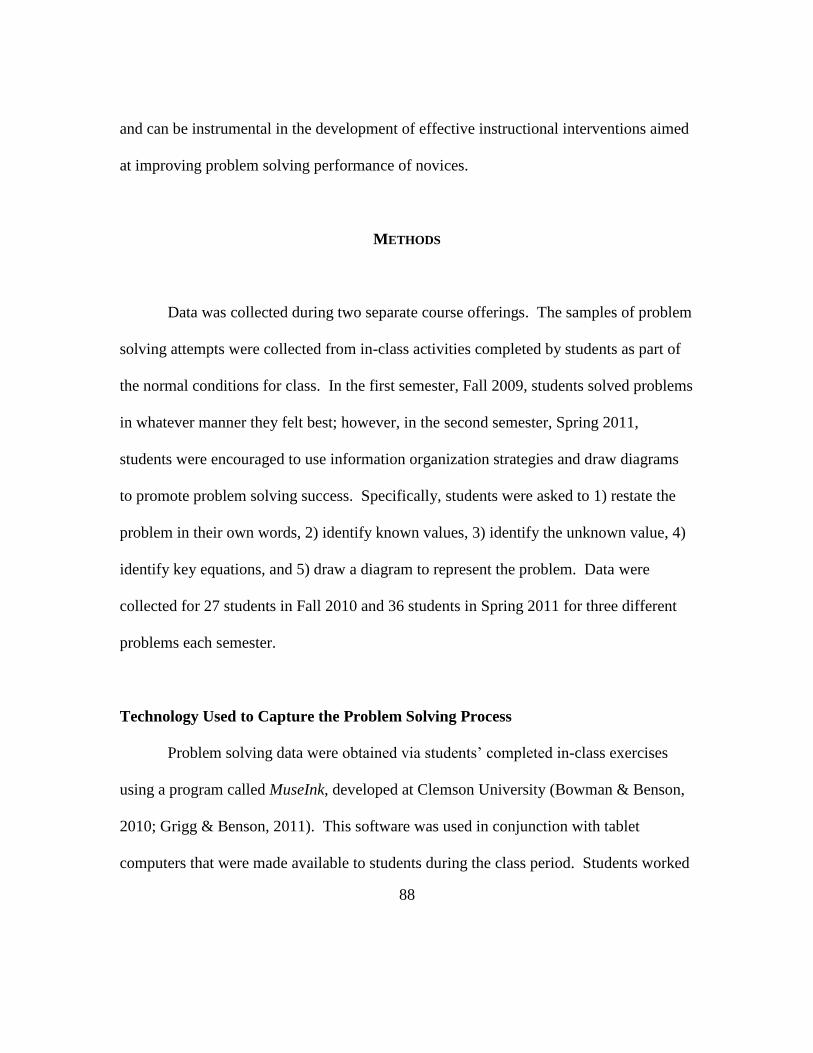
88

and can be instrumental in the development of effective instructional interventions aimed

at improving problem solving performance of novices.

METHODS

Data was collected during two separate course offerings. The samples of problem

solving attempts were collected from in-class activities completed by students as part of

the normal conditions for class. In the first semester, Fall 2009, students solved problems

in whatever manner they felt best; however, in the second semester, Spring 2011,

students were encouraged to use information organization strategies and draw diagrams

to promote problem solving success. Specifically, students were asked to 1) restate the

problem in their own words, 2) identify known values, 3) identify the unknown value, 4)

identify key equations, and 5) draw a diagram to represent the problem. Data were

collected for 27 students in Fall 2010 and 36 students in Spring 2011 for three different

problems each semester.

Technology Used to Capture the Problem Solving Process

Problem solving data were obtained via students’ completed in-class exercises

using a program called MuseInk, developed at Clemson University (Bowman & Benson,

2010; Grigg & Benson, 2011). This software was used in conjunction with tablet

computers that were made available to students during the class period. Students worked

89

out problems in the MuseInk application, which digitally records ink strokes and keeps a

running log of the entire solution process from beginning to end, including erasures, and

can be replayed and coded directly in the application at any point in time.

Engineering Problems

The three problems analyzed covered the topics of 1) efficiency, 2) circuits, and

3) pressure. All problems had 1) a constrained context, including pre-defined elements

(problem inputs), 2) allowed multiple predictable procedures or algorithms, and 3) had a

single correct answer (Jonassen, 2004). All three problems were story problems, in

which the student is presented with a narrative that embeds the values needed to obtain a

final answer (Jonassen, 2010). The first problem involved a multi-stage solar energy

conversion system and required calculation of the efficiency of one stage given input and

output values for the other stages (Stephan, Park, Sill, Bowman, & Ohland, 2010). The

second problem required students to solve for values of components in a given electrical

circuit. This problem, developed by the project team, also contained a Rule-Using/Rule

Induction portion (a problem having one correct solution but multiple rules governing

the process (Jonassen, 2010)), where students were asked to determine an equivalent

circuit based on a set of given constraints. The third problem involved hydrostatic

pressure in a vessel, and required students to solve for values within the system, and

convert between different unit systems (Stephan, et al., 2010). The problems are

included in Appendices A-C.

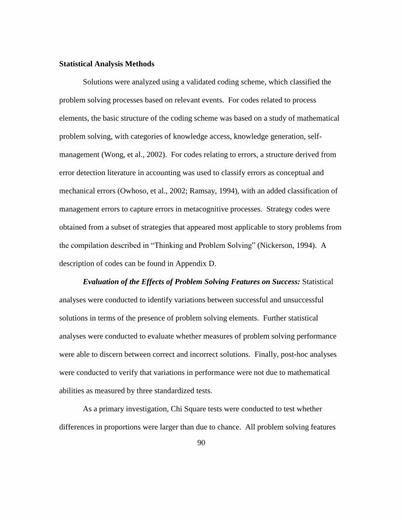
90

Statistical Analysis Methods

Solutions were analyzed using a validated coding scheme, which classified the

problem solving processes based on relevant events. For codes related to process

elements, the basic structure of the coding scheme was based on a study of mathematical

problem solving, with categories of knowledge access, knowledge generation, self-

management (Wong, et al., 2002). For codes relating to errors, a structure derived from

error detection literature in accounting was used to classify errors as conceptual and

mechanical errors (Owhoso, et al., 2002; Ramsay, 1994), with an added classification of

management errors to capture errors in metacognitive processes. Strategy codes were

obtained from a subset of strategies that appeared most applicable to story problems from

the compilation described in “Thinking and Problem Solving” (Nickerson, 1994). A

description of codes can be found in Appendix D.

Evaluation of the Effects of Problem Solving Features on Success: Statistical

analyses were conducted to identify variations between successful and unsuccessful

solutions in terms of the presence of problem solving elements. Further statistical

analyses were conducted to evaluate whether measures of problem solving performance

were able to discern between correct and incorrect solutions. Finally, post-hoc analyses

were conducted to verify that variations in performance were not due to mathematical

abilities as measured by three standardized tests.

As a primary investigation, Chi Square tests were conducted to test whether

differences in proportions were larger than due to chance. All problem solving features

91

occurring at least once in the problem solving attempts were classified as occurring, even

if the work was later modified to eliminate its presence in the final solution. Then, odds

ratios were calculated to determine how much more likely a successful or unsuccessful

solution was to contain a particular feature. For this analysis, each solution was treated

as an independent sample to approximate general trends.

A secondary analysis was conducted in order to evaluate the predictive value of

specific problem solving features on problem solving success while taking into account

anomalies that may have occurred because solutions were not independent samples, as

the same student completed up to three solutions. Linear mixed-effect models were used

to verify the relationships to problem solving success after accounting for variations due

to the problem, the semester, and the participant. The factor of “semester” is being used

as a proxy measure of the effect of the pedagogical intervention in the second semester.

Evaluation of Performance Measures and their Relationships to Problem

Solving Success: In an effort to validate the proposed performance measures, statistical

analyses were conducted to evaluate whether the transformed data was associated with

and able to predict successful solution outcomes. Twenty-eight internal process measures

of students’ problem solving methods and skills utilized along Sternberg’s seven stage

problem solving cycle were evaluated (Pretz, et al., 2003). Five outcome measures were

also evaluated as a means of validating that they are acceptable predictors of success.

Performance measures and their calculations are included in Appendix E.

Similar to the analysis methods of problem solving features, Chi Squared tests

92

were conducted to compare differences in performance measures of categorical nature

and Wilcoxon sum rank tests were conducted on performance measures that were of

interval or ratio data types, using the Chi Squared approximation to determine the level of

significance. As before, repeated measures analyses were conducted using linear mixed-

effects models to assess the predictive strength of performance measures after taking into

account effects due to the problem, semester, and the participant.

RESULTS

Effects of Planning and Visualization Activities

Results indicated that problem solving success was improved by encouraging

information organization and problem representation tasks, as there was a significant

increase in the success rate for the semester when the intervention occurred (p=0.001).

During the Fall 2009 semester, when students completed problems in their preferred

manner, only 21% of solutions were 100% correct. During the Spring 2011 semester,

when students were encouraged to use information organization and problem

representation strategies, 80% of solutions were 100% correct.

An analysis of problem definition and representation strategies present on the

Spring 2011 data in isolation showed significant effects on successful solutions when

planning tasks were completed in the first half of the solution attempt (Grigg & Benson,

2012). Results revealed that when students completed a planning phase that involved

93

restating the problem, identifying known values, identifying the unknown value, and

explicitly identifying relevant equations during the first half of their problem solving

attempt (n = 28 of 76), solutions were more likely to include correct answers (p = 0.05).

Figure 6.1 illustrates the use of a complete planning phase and the resulting correct

solution while Figure 6.2 illustrates an incomplete planning phase and the resulting

incorrect solution. Unfortunately, this analysis cannot be compared with the Fall 2009

data, as no one completed all of the problem definition tasks by choice.

Figure 6.1: A correct solution utilizing a complete planning phase: restating the problem,

identifying known values, identifying unknown values, and identifying equations

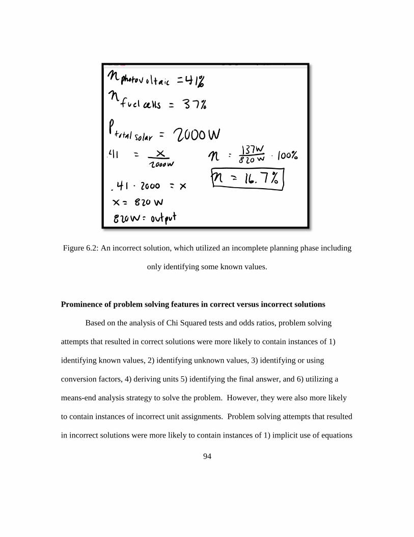
94

Figure 6.2: An incorrect solution, which utilized an incomplete planning phase including

only identifying some known values.

Prominence of problem solving features in correct versus incorrect solutions

Based on the analysis of Chi Squared tests and odds ratios, problem solving

attempts that resulted in correct solutions were more likely to contain instances of 1)

identifying known values, 2) identifying unknown values, 3) identifying or using

conversion factors, 4) deriving units 5) identifying the final answer, and 6) utilizing a

means-end analysis strategy to solve the problem. However, they were also more likely

to contain instances of incorrect unit assignments. Problem solving attempts that resulted

in incorrect solutions were more likely to contain instances of 1) implicit use of equations

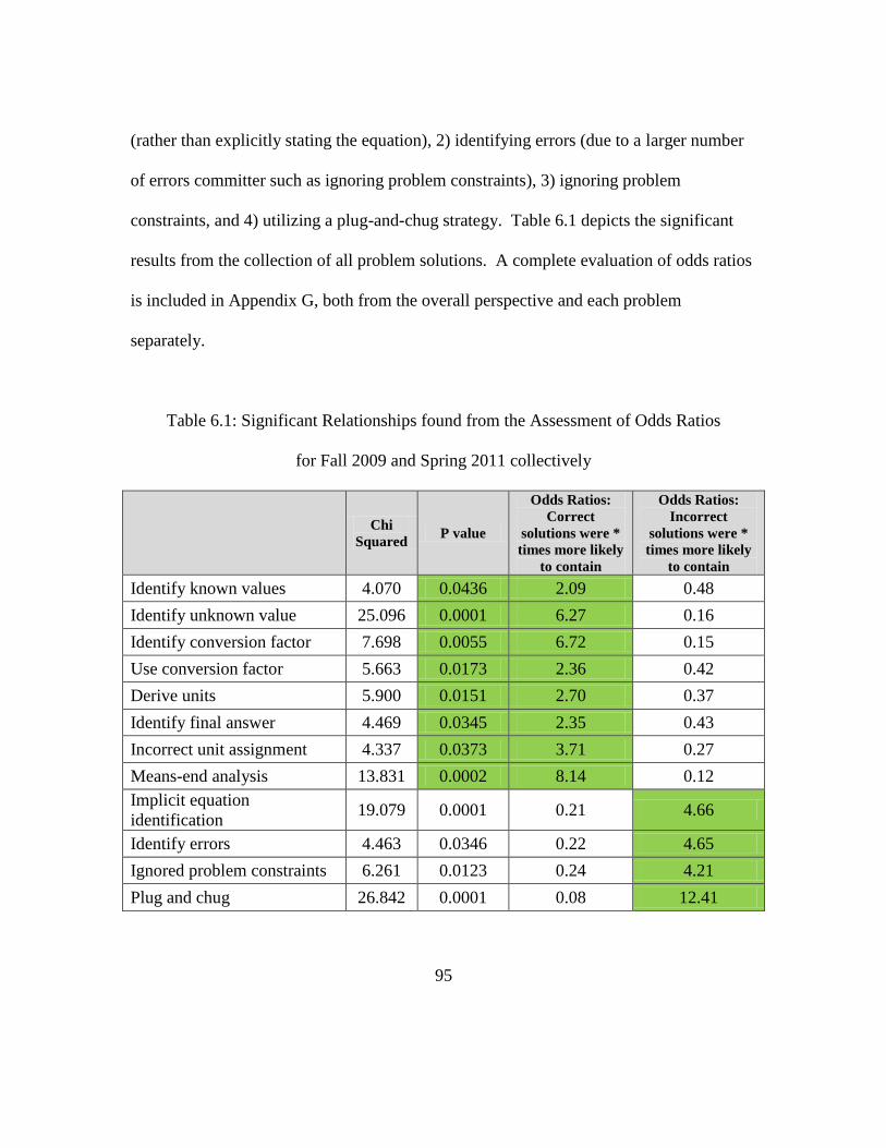
95

(rather than explicitly stating the equation), 2) identifying errors (due to a larger number

of errors committer such as ignoring problem constraints), 3) ignoring problem

constraints, and 4) utilizing a plug-and-chug strategy. Table 6.1 depicts the significant

results from the collection of all problem solutions. A complete evaluation of odds ratios

is included in Appendix G, both from the overall perspective and each problem

separately.

Table 6.1: Significant Relationships found from the Assessment of Odds Ratios

for Fall 2009 and Spring 2011 collectively

Chi

Squared P value

Odds Ratios:

Correct

solutions were *

times more likely

to contain

Odds Ratios:

Incorrect

solutions were *

times more likely

to contain

Identify known values 4.070 0.0436 2.09 0.48

Identify unknown value 25.096 0.0001 6.27 0.16

Identify conversion factor 7.698 0.0055 6.72 0.15

Use conversion factor 5.663 0.0173 2.36 0.42

Derive units 5.900 0.0151 2.70 0.37

Identify final answer 4.469 0.0345 2.35 0.43

Incorrect unit assignment 4.337 0.0373 3.71 0.27

Means-end analysis 13.831 0.0002 8.14 0.12

Implicit equation

identification 19.079 0.0001 0.21 4.66

Identify errors 4.463 0.0346 0.22 4.65

Ignored problem constraints 6.261 0.0123 0.24 4.21

Plug and chug 26.842 0.0001 0.08 12.41

96

Next, problem solving features were evaluated using linear mixed-effects models

to calculate the significant effects on success while taking into account variability

attributable to the problem, and the semester as well as random effects of the person.

While it was expected that a majority of the significant effects would mimic those

observed via Chi Squared tests, only two of the effects of problem solving tasks and two

of the effects of strategies remained the same. It was evident that the problem and the

semester had significant effects on all analyses, with the second problem being associated

with lower success rates and the second semester (the intervention group) being

associated with higher success rates. Based on the regression models, additional problem

solving features associated with successful solutions included 1) documenting math and

2) utilizing a chunking strategy. Additional problem solving features associated with

incorrect solutions included 1) labeling and renaming, 2) incorrectly relating variables,

and 3) inconsistent units. The use of problem solving features such as identifying known

values, identifying unknown values, and identifying conversion factors were likely

attributed to effects of the semester rather than success as most all students in the second

semester utilized those features and were no longer found to have significant effects. The

additional significant effects found for errors were likely associated with specific

problems, and were not found to be significant until the effects of the problems were

taken into account. A summary of significant effects is shown in Table 6.2 and a detailed

description of the linear mixed-effects models is included in Appendix H.

97

Table 6.2: Summary of significant effects influencing problem solving success

Arrows indicate the directionality of the effect. Up arrows indicate positive correlations

with success (100% correct solutions) and down arrows indicate negative associations.

Problem Solving Features Problem Solving Success

Tasks

Use conversion factor

Document math Labeling / Renaming

Identify errors

Errors Incorrectly relate variables

Inconsistent units

Strategies

Plug and Chug

Means-ends-analysis

Chunking

Are the Performance Measures Predictive of Problem Solving Success?

When correct and incorrect solutions were compared in terms of internal process

measures of performance, several significant findings emerged that indicated which

actions were associated with problem solving success. Findings showed that explicitly

identifying the unknown value, explicitly (and correctly) defining the problem, and

explicitly writing out known values and equations were all related to correct solutions. In

addition, using intermediate or advanced level strategies, rather than strategies of guess

and check or plug-and-chug, were related to correct solutions. Utilizing more knowledge

generation tasks, executing correct mechanical manipulations, and indicating the final

answer were also related to correct solutions; however it was also related to a more

98

problem elements overall. One of the most highly correlated performance measures was

the accuracy of identifying errors as measured through the hit rate and sensitivity scores.

Table 6.3 reports the findings of the tests of process measures along with the mean values

and significance level of differences. Four of the five outcome measures had significant

effects in association with success. Management errors and time to completion did not

have significant relationships to success. Table 6.4 reports the findings of the tests of

outcome measures along with the mean values and significance level of differences.

Next, performance measures were evaluated using linear mixed-effects models to

calculate the significant effects on success while taking into account variability

attributable to the problem and the semester, as well as random effects of the person.

Eight of the relationships disappear when accounting for effects of differences across

semester and random effects of the person. Four additional significant effects emerged.

The shift appeared to navigate away from the significant effects of explicit expressions in

favor of correct execution of those tasks. This indicates that the explicit expression of

tasks may be more useful for specific individuals, but overall, the accuracy of those

expressions is most significant to problem solving success. In addition, relationships

between success and all outcome measures were significant except for time to

completion. A summary of significant effects are shown in Tables 6.5-6.6 and the

extended results are shown in Appendices I-J.

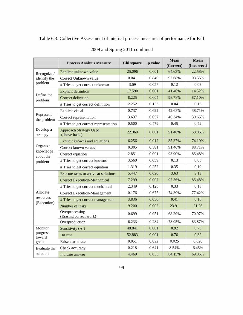
99

Table 6.3: Collective Assessment of internal process measures of performance for Fall

2009 and Spring 2011 combined

Process Analysis Measure Chi square p value Mean

(Correct)

Mean

(Incorrect)

Recognize /

identify the

problem

Explicit unknown value 25.096 0.001 64.63% 22.58%

Correct Unknown value 0.041 0.840 92.68% 93.55%

# Tries to get correct unknown 3.69 0.057 0.12 0.03

Define the

problem

Explicit definition 17.590 0.001 41.46% 14.52%

Correct definition 8.225 0.004 98.78% 87.10%

# Tries to get correct definition 2.252 0.133 0.04 0.13

Represent

the problem

Explicit visual 0.737 0.692 42.68% 38.71%

Correct representation 3.637 0.057 46.34% 30.65%

# Tries to get correct representation 0.500 0.479 0.45 0.42

Develop a

strategy

Approach Strategy Used

(above basic) 22.369 0.001 91.46% 58.06%

Organize

knowledge

about the

problem

Explicit knowns and equations 6.256 0.012 85.37% 74.19%

Correct known values 0.305 0.581 91.46% 88.71%

Correct equation 2.851 0.091 93.90% 85.48%

# Tries to get correct knowns 3.560 0.059 0.13 0.05

# Tries to get correct equation 1.319 0.252 0.35 0.19

Allocate

resources

(Execution)

Execute tasks to arrive at solutions 5.447 0.020 3.63 3.13

Correct Execution-Mechanical 7.299 0.007 97.56% 85.48%

# Tries to get correct mechanical 2.349 0.125 0.33 0.13

Correct Execution-Management 0.176 0.675 74.39% 77.42%

# Tries to get correct management 3.836 0.050 0.41 0.16

Number of tasks 9.200 0.002 23.91 21.26

Overprocessing

(Erasing correct work) 0.699 0.951 68.29% 70.97%

Overproduction 6.233 0.284 78.05% 83.87%

Monitor

progress

toward

goals

Sensitivity (A’) 48.841 0.001 0.92 0.73

Hit rate 52.883 0.001 0.76 0.32

False alarm rate 0.051 0.822 0.025 0.026

Evaluate the

solution

Check accuracy 0.218 0.641 8.54% 6.45%

Indicate answer 4.469 0.035 84.15% 69.35%

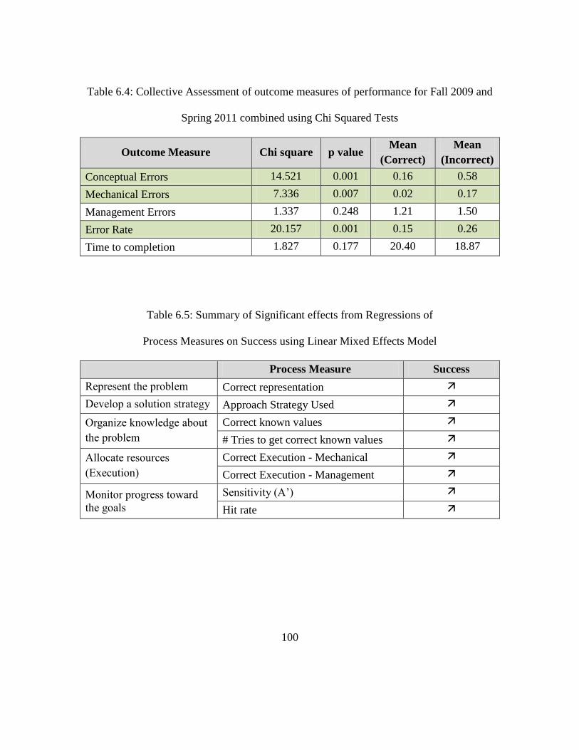
100

Table 6.4: Collective Assessment of outcome measures of performance for Fall 2009 and

Spring 2011 combined using Chi Squared Tests

Outcome Measure Chi square p value Mean

(Correct)

Mean

(Incorrect)

Conceptual Errors 14.521 0.001 0.16 0.58

Mechanical Errors 7.336 0.007 0.02 0.17

Management Errors 1.337 0.248 1.21 1.50

Error Rate 20.157 0.001 0.15 0.26

Time to completion 1.827 0.177 20.40 18.87

Table 6.5: Summary of Significant effects from Regressions of

Process Measures on Success using Linear Mixed Effects Model

Process Measure Success

Represent the problem Correct representation

Develop a solution strategy Approach Strategy Used

Organize knowledge about

the problem

Correct known values

# Tries to get correct known values

Allocate resources

(Execution)

Correct Execution - Mechanical

Correct Execution - Management

Monitor progress toward

the goals

Sensitivity (A’)

Hit rate

101

Table 6.6: Summary of Significant effects from Regressions of

Outcome Measures on Success using Linear Mixed Effects Model

Outcome Measure Success

Conceptual Errors

Mechanical Errors

Management Errors

Error Rate

DISCUSSION

There was a dramatic improvement in the problem solving success rate of

students in the Spring 2011 semester, who were asked to utilize information organization

and visualization tasks, over the Fall 2009 semester, where students were left to construct

problem solutions as they saw fit. When comparisons were made that accounted for

random effects of the students and fixed effects of the problem and the semester, the

semester was a significant indicator of success at the p< 0.001 level. At first, it was

believed that there might have been a discrepancy between semesters with the

intervention group having more advanced mathematics skills. However a post hoc

review of standardized test scores on the SAT math portion, CMPT (Clemson Math

Placement Test), and BST (Basic Skills Test) showed that the intervention group actually

had lower average test scores for the SAT math portion (p=0.009) and the CMPT

(p=0.009) and there was not a statistically significant difference between groups on the

102

BST. Therefore, the more successful problem solving performance was not likely to be

due to mathematics skills, reaffirming that there was, indeed, a positive impact from of

implementing this problem solving structure.

Comparisons of student problem solving attempts revealed that explicitly writing

out information seemed to improve the chances of achieving correct solutions for many

students. Yet, when variability due to the student was taken into account, the accuracy of

the information was more closely related to success. It is possible that, in some cases,

simply going through the task of identifying information oriented students to the solution

path. On a related note, some students were able to overcome errors (especially

management errors) to arrive at correct solutions despite the errors evident in their

solutions; however, this was highly dependent on effects of the student. On the other

hand, more detrimental effects occurred from conceptual or mechanical errors. It also

appears that some students need to rely on writing out each step of their algebraic

manipulations (documenting work) more than others do, as this effect disappears when

random effects of the student are taken into account.

Correct visual representations of the system were also found to be associated to

problem solving success when taking into account effects of the problem, semester, and

students, though these factors all play a role in how useful the diagram is. It is important

to note that correct visual representations were considered only for those that established

correct relationships between variables in addition to a pictorial aspect.

It was also revealed that making errors (especially incorrectly relating variables,

103

ignoring problem constraints, or having inconsistent units within the documented work)

were associated with incorrect solutions. However, simply making an error did not

necessarily lead to an incorrect solution, as many students who achieved correct solutions

made errors, but were able to correct them, even if it took multiple attempts. In fact, one

of the most significant factors in problem solving success were the measures of

sensitivity and hit rate, or the correct identification of errors. Therefore, instructors have

an opportunity to help students enhance problem solving performance by encouraging the

development of error identification skills.

Another key differentiator between correct and incorrect solutions was the

approach taken to solving the problem. While a chunking strategy was associated with

correct solutions, the approach may not be practical for all students as it is considered an

advanced strategy; novice problem solvers may not have the cognitive resources to

employ this strategy. However, means-ends-analysis, considered an intermediate

strategy, was also highly correlated to problem solving success, while a plug-and-chug

strategy, a lower level strategy, was highly correlated to incorrect solutions. This

highlights the need for instructors to work with students on developing plans for the

execution of problem solving tasks.

104

CONCLUSION

This research suggests some techniques that instructors may use to encourage

problem solving success. Encouraging planning activities had a positive impact on

student problem solving success for the problems included in this analysis. However,

instructors should emphasize the benefits of restating the problem in their own words

before identifying known values, unknown values, and equations. The interconnectivity

of these processes should be emphasized. Students may also benefit from returning to

restate the problem as a means of overcoming impasses or errors in the problem solving

attempts as errors made in the planning phase can have detrimental effects throughout the

remainder of the solution. On a related note, instructors should also emphasize error

identification.

While many instructors may be eager simply to instruct students to utilize these

techniques, students will likely resist unless there is a formal explanation of the benefits.

For example, students in the Spring 2011 semester often restated the problem, identified

known values, identified the unknown values, and identified relevant equations after

completing the problem simply to fulfill those requirements, reducing the effectiveness of

the planning activity (and likely also reducing the statistical power assigned to those

codes in this analysis). Only 36.8% of solutions utilized the planning activities as

intended despite over 70% of students eventually completing the tasks. It is suggested

that instructors explicitly teach problem solving methods to inform students of the value

105

of these planning activities rather than simply requiring their use to have the greatest

impact on student learning.

One possible way of encouraging these planning activities and development of

error identification skills is to conduct an in-class activity where students detail the

system from different problems and swap the problem setups with other students who in

turn evaluate the setups for accuracy (independent of knowledge generation tasks). An

alternative is for instructors to break down the problem into multiple parts, where

students have to transition through the problem solving process as they progress through

the problem. For example, having “Part A” to define and represent the problem, before

transitioning into “Part B” where students execution tasks to solve for the unknown value

and “Part C” where students reflect on their answer and justify their method and/or

solution. Leading the student through a multi-step solution may help teach students how

they should approach problem solutions. However, this strategy would likely be most

effective if students were made aware of the purpose of the guided solution and would be

most effective when taught in conjunction with problem solving strategies. In this

situation, instructors can explicitly address problems in student methods by assessing

their problem solving skills on performance measures such as those utilized in this

manuscript. Receiving a record of problem solving skills deficiencies may help students

raise metacognitive awareness and serve to pinpoint areas of instructional need. The

development of a rubric for this purpose is discussed in Chapter 9.

106

CHAPTER SEVEN

WHAT ARE THE RELATIONSHIPS BETWEEN PROBLEM SOLVING

PERFORMANCE AND MENTAL WORKLOAD?

Some variation between expert and novice problem solving performance has been

explained by strain on novices’ cognitive resources. This research shows how a self-

reported workload measure, the NASA-TLX, can be used to assess task difficulty and

serve as an indicator of performance deficiencies. Additionally, by comparing problem

solving features and performances to NASA-TLX scores, relationships can be identified

that are linked to lower mental workload scores, which can inform instructional

interventions to help struggling students overcome cognitive overload.

Three relatively well-structured story problems of varying complexity were

analyzed for submissions made by 36 students. Results confirmed that higher probability

of success were moderately correlated to lower average task load index scores as well as

subscales of temporal demand, performance, effort, and frustration. These results

confirm that the NASA-TLX can serve as a potential alternative means of assessing task

difficulty with additional benefits of alluding to sources of problem difficulty.

When assessing problem solving features in terms of mental workload measures,

it was found that two processes, six errors, and one approach strategy were associated

with higher mental workloads while two tasks and two approach strategies were

associated with lower mental workload. Twelve performance measures were associated

107

with significant effects on mental workload measures; four were associated with lower

mental workload measures with eight associated with higher mental workload. Effects

on mental workload must be interpreted with caution as highest levels of performance are

associated with mid-level mental workload scores, so extreme high or extreme low

mental workload can both be detrimental.

INTRODUCTION

Problem solving skills are critical for engineers as they are tasked with tackling

some of the most pressing global challenges (Perry, et al., 2008). Because of the

importance of problem solving skills, educators should strive to help students obtain

knowledge resources and develop skills required for problem solving success. However,

problem solving is a complex activity, modeled as a seven stage process: 1) recognize /

identify the problem, 2) define and represent the problem, 3) develop a solution strategy,

4) organize knowledge about the problem, 5) allocate resources for solving the problem,

6) monitor progress toward the goals, and 7) evaluate the solution for accuracy (Pretz, et

al., 2003). In practice, there is much variability in how people approach the problem

solving process. The stages are not utilized by all problem solvers in all situations, and

the problem solver may iterate between stages as s/he responds to feedback, either

internal or external (Wilson, et al., 1993). It is possible for students to have proficiency

in parts of the problem solving cycle but have limitations on other stages.

108

Yet, typically, success is measured by outcomes, such as solution accuracy

(Drury, 1990), which may not give a true measure of a student skills levels. For example,

something as minor as a calculation error caused by accidentally pressing the incorrect

number on a calculator can lead to an incorrect solution despite knowing how to complete

the problem; and yet, a student can obtain the correct answer by following how someone

else completes the problem without knowing how to solve it independently.

In the search for behaviors that promote problem solving proficiency, research has

classified variations in performance between expert and novice problem solvers (Chi, et

al., 1988) presumably because experts’ problem solutions exhibit more successful

application of problem solving skills. However, methods used by experts to solve

problems are not necessarily transferable to novices due to cognitive requirements

necessary to use these strategies (Wang & Chiew, 2010). Low cognitive workload

capacity has been linked to the use of inefficient approaches, lacking relevant information

necessary to solve the problem, and lacking awareness of performance errors (Wang &

Chiew, 2010) while higher cognitive workload capacity is predictive of higher

performance and the ability to overcome impasses in problem solving (Hambrick &

Engle, 2003). If a student’s workload capacity is low, then (s)he may lack enough excess

capacity to encode new knowledge thus hindering learning (Sweller, 1988).

Some of the factors that have been shown to contribute to cognitive load include

the number of tasks to be performed, the need for accuracy, time pressure, and cognitive

capacities of the individual (Proctor & Van Zandt, 2008). Researchers have

109

recommended writing things down as a means of reducing cognitive load during the

problem solving process (Woods, et al., 2000). This research investigates the

relationships between problem solving features, errors, and strategies evident in students’

written work with cognitive (mental) workload of first year engineering students in an

effort to identify recommendations that may help students suffering from cognitive

overload. In addition, problem solving performance measures along the problem solving

cycle were analyzed in terms of cognitive load to evaluate whether certain problem

solving processes contribute to cognitive load at a higher rate than others.

Assessing Cognitive (Mental) Workload

Mental workload measures assess how draining the task was on the student’s

cognitive resources (Drury, 1990). Human factors literature offers several ways of

assessing mental workload including primary task, secondary task, psychophysiological,

and self-report measures (Wilson & Corlett, 2005). Self-report assessments lend

themselves as the most practical measure based on their unobtrusive nature, ease of

assessment, and quick data collection. The three most widely used subjective measures

of mental workload are 1) the Modified Cooper-Harper scale, 2) Subjective Workload

Assessment Technique (SWAT) and 3) NASA-Task Load Index (NASA-TLX). All three

assessments are generic, can be applied to any domain, and are not obtrusive to task

performance when administered after the task (Stanton, et al., 2005).

110

The Modified Cooper-Harper Scale assesses difficulty level on a ten-item scale

from very easy to impossible based on a classification of the demand level placed on the

operator. Accurate assessment requires the operator to carefully read each option and

make fine distinctions between ratings of mental effort and ability to thwart errors

(Wilson & Corlett, 2005). In addition, it cannot be used to diagnose sources of workload

stress (Farmer & Brownson, 2003).

The SWAT is a three item scale that rates time load, mental effort load, and

psychological stress load on scales of 1-3. The scales do not easily translate to problem

solving tasks because the assessment is geared toward tasks that take extensive time. For

example, time load is measured on the three point scale: 1= Often have spare time,

2=Occasionally have spare time, and 3=Almost never have spare time. Additionally,

SWAT has been criticized for being insensitive to low mental workloads (Stanton, et al.,

2005) and has not been empirically validated (Farmer & Brownson, 2003).

The NASA-TLX consists of six subscales, three measuring demand put on the

participant by the task and three measuring stress added by the worker as a result of

interacting with the task. The NASA-TLX subscales are scored on a continuous scale

from zero to twenty (Hart, 2006; Stanton, et al., 2005). The NASA-TLX has been noted

as highly reliable, extensively validated, has a high sensitivity, can be used to diagnose

sources of workload and takes 1-2 minutes to complete (Farmer & Brownson, 2003). For

these reasons, the NASA-TLX was chosen as the tool for assessing mental workload for

this research effort.

111

METHODS

This research explores relationships between mental workload and problem

solving features and performance measures. Tablet PCs were used to capture student

problem solving attempts and students completed the NASA-TLX survey immediately

following completion of the problem solving tasks.

Technology Used to Capture Problem Solving Processes

Problem solving data was obtained via students’ completed in-class exercises

using a program called MuseInk, developed at Clemson University (Bowman & Benson,

2010; Grigg & Benson, 2011). This software was used in conjunction with tablet

computers that were made available to all students during the class period. MuseInk files

(.mi) keep a running log of the entire problem solution process from beginning to end,

including erasures, and can be replayed and coded directly in the application at any point

in time on the data file. The software enables the researcher to associate codes to the

problem solution at any point, even to erased work.

Solutions were analyzed using a validated coding scheme developed by the

research group, which classified the problem solving processes based on relevant events.

Cognitive and metacognitive tasks were classified into categories based on a theoretical

framework of process activities used during mathematical problem solving (Wong, et al.,

2002): knowledge access, knowledge generation and self-management. For codes relating

112

to errors, a structure derived from error detection literature in accounting, was used to

classify errors as conceptual and mechanical errors (Owhoso, et al., 2002; Ramsay, 1994)

with an added classification of management errors to capture errors in metacognitive

processes. Strategy codes were obtained from a subset of strategies that appeared most

applicable to story problems from the compilation described in “Thinking and Problem

Solving” (Nickerson, 1994).

Engineering Problems under Analysis

Three problems were analyzed which covered the topics of 1) solar power system

efficiency, 2) electrical circuits, and 3) hydrostatic pressure. All problems had 1) a

constrained context, including pre-defined elements (problem inputs), 2) allowed

multiple predictable procedures or algorithms, and 3) had a single correct answer

(Jonassen, 2004). All three problems were story problems, in which the student is

presented with a narrative that embeds the values needed to obtain a final answer

(Jonassen, 2010). The first problem involved a multi-stage solar energy conversion

system and required calculation of the efficiency of one stage given input and output

values for the other stages (Stephan, et al., 2010). The second problem required students

to solve for values of components in a given electrical circuit. This problem, developed

by the project team, also contained a Rule-Using/Rule Induction portion (a problem

having one correct solution but multiple rules governing the process (Jonassen, 2010)),

where students were asked to determine an equivalent circuit based on a set of given

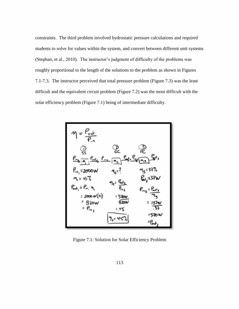
113

constraints. The third problem involved hydrostatic pressure calculations and required

students to solve for values within the system, and convert between different unit systems

(Stephan, et al., 2010). The instructor’s judgment of difficulty of the problems was

roughly proportional to the length of the solutions to the problem as shown in Figures

7.1-7.3. The instructor perceived that total pressure problem (Figure 7.3) was the least

difficult and the equivalent circuit problem (Figure 7.2) was the most difficult with the

solar efficiency problem (Figure 7.1) being of intermediate difficulty.

Figure 7.1: Solution for Solar Efficiency Problem

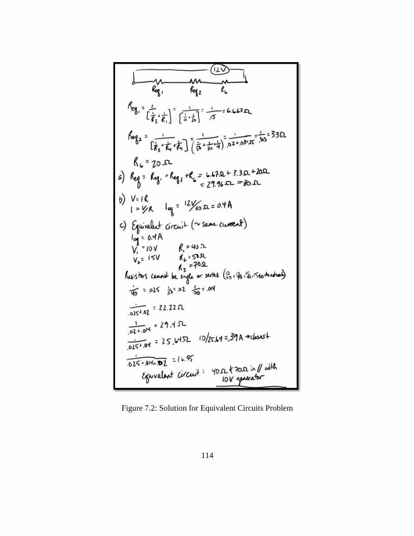
114

Figure 7.2: Solution for Equivalent Circuits Problem

115

Figure 7.3: Solution for Total Pressure Problem

NASA-TLX survey

The NASA-TLX consists of six subscales, three measuring demand put on the

participant by the task and three measuring stress added by the worker as a result of

interacting with the task. The three measures of task demand include 1) mental demand,

2) physical demand, and 3) temporal demand. The remaining measures, 4) effort, 5)

performance, and 6) frustration, describe the stress put on the person by the interaction of

the person with the task (Warm, et al., 2008). Table 7.1 summarizes the survey items.

116

The NASA-TLX subscales are scored on a continuous scale from zero to twenty. The

overall mental workload is calculated by adding together the scores of the individual

subscales (Stanton, et al., 2005). For this study, the physical demand subscale was not

utilized in calculating the overall mental workload score. The comparison of individual

subscale values has become acceptable practice and has been conducted by a variety of

researchers in order to evaluate contributors to workload stress (Hart, 2006).

Table 7.1: Items of the NASA-TLX survey (NASA)

Mental Demand How mentally demanding was the task?

Physical Demand How physically demanding was the task?

Temporal Demand How hurried or rushed was the pace of the task?

Performance How successful were you in accomplishing what

you were asked to do?

Effort How hard did you have to work to accomplish your

level of performance?

Frustration How insecure, discouraged, irritated, stressed, and

annoyed were you?

Statistical Analysis

First, to investigate the appropriateness of the NASA-TLX as a measure of

problem solving difficulty, the mean mental workload scores were compared to each

student’s probability of obtaining a correct answer for each problem. Then, Spearman’s

rho rank correlational coefficients were calculated to assess the level of association

117

between solution accuracy and individual subscales of mental workload. Non-parametric

tests were utilized because answer accuracy was not normally distributed for this sample,

though measures of mental workload were normally distributed.

Next, the effects of various problem solving features on mental workload were

evaluated. Repeated measures analyses were conducted, using a linear mixed-effects

model (Seltman, 2012) to assess significant effects of completing a task, making an error,

or using a strategy while taking into account extraneous factors such as the problem and

the participant. Analyses were conducted on 46 codes of process elements, errors, and

strategies, shown in Appendix D.

Finally, the effects of problem solving features were evaluated in terms of

differences in mental workload as a secondary measures of their predictive ability

(success was assessed in Chapter 6 as the primary measure). Repeated measures analyses

were conducted using linear mixed-effects models to evaluate the effect of performance

on measures of mental workload and workload subscales while taking into account

extraneous factors of the problem and the person. Solutions were evaluated on 28

internal process measures of students’ problem solving skills organized according to

Sternberg’s seven stage problem solving cycle as well as six additional metrics that

measure the outcomes in terms of speed and accuracy. Performance measures and their

calculations are shown in Appendices E-F.

118

RESULTS

Comparing solution accuracy with mental workload measures

Average mental workload scores and the probability of success were calculated

for each of the three problems. Ideally, average perceived mental workload scores would

fall just slightly above 50 to indicate that the problems were challenging yet achievable,

though students reported levels slightly below and achieved higher levels of success than

expected. As shown in Table 7.2, there is an apparent inverse relationship between

mental workload and probability of success; when more students obtained the correct

answer, average scores of mental workload were lower. However, all three problems

resulted in similar scores for mental workload and for probability of success. Therefore,

few definitive conclusions can be drawn from the average scores, except that the three

problems appear to be approximately equal in terms of difficulty.

Table 7.2: Summary of mean Mental Workload Scores and success rates

Solar Efficiency

Problem

Equivalent Circuit

Problem

Total Pressure

Problem

Sample Size (n=26) (n=21) (n=24)

Probability of success 0.88 0.89 0.92

NASA-TLX 5 47.04 43.54 41.91

Next, the relationship between mental workload and level of solution accuracy

was assessed for the entire sample of seventy-one solutions. For the overall sample,

significant effects were found between solution accuracy and measures of mental

119

workload and all subscales except mental demand. Moderate correlations were found

between level of success and ratings of frustration (ρ = - 0.30), performance (ρ = -0.27),

effort (ρ = - 0.26), temporal demand (ρ = - 0.26), and overall mental workload score (ρ =

-0.24) with higher accuracy levels correlated to lower mental workload scores. A

summary of results is shown in Table 7.3.

Table 7.3: Pearson correlation coefficients of the relationships between

mental workload scores and the probability of success

Spearman’s rho P value

NASA-TLX 5 -0.24 0.044

Mental Demand -0.05 0.706

Temporal Demand -0.26 0.031

Performance -0.27 0.021

Effort -0.26 0.029

Frustration -0.30 0.011

Exploring relationships between problem solving features and mental workload

scores

Repeated measures analyses were conducted using a linear mixed effects model to

calculate the effects on mental workload using fixed effects of the problem and the task

element/error/strategy under question as well as accounting for random effects attributed

to the student. Several of the regression models revealed differences attributable to the

problem, indicating that relationships may vary based on the characteristics of the

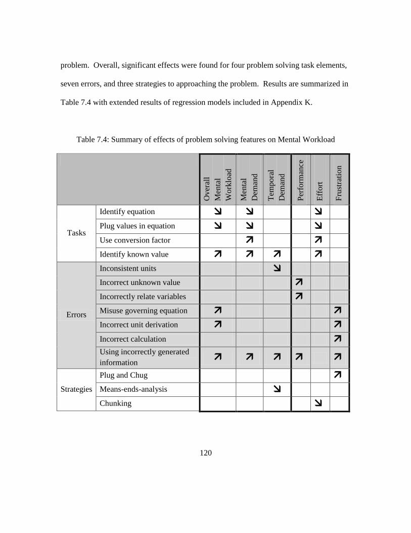
120

problem. Overall, significant effects were found for four problem solving task elements,

seven errors, and three strategies to approaching the problem. Results are summarized in

Table 7.4 with extended results of regression models included in Appendix K.

Table 7.4: Summary of effects of problem solving features on Mental Workload

Over

all

Men

tal

Work

load

Men

tal

Dem

and

Tem

pora

l

Dem

and

Per

form

ance

Eff

ort

Fru

stra

tion

Tasks

Identify equation

Plug values in equation

Use conversion factor

Identify known value

Errors

Inconsistent units

Incorrect unknown value

Incorrectly relate variables

Misuse governing equation

Incorrect unit derivation

Incorrect calculation Using incorrectly generated

information

Strategies

Plug and Chug

Means-ends-analysis

Chunking

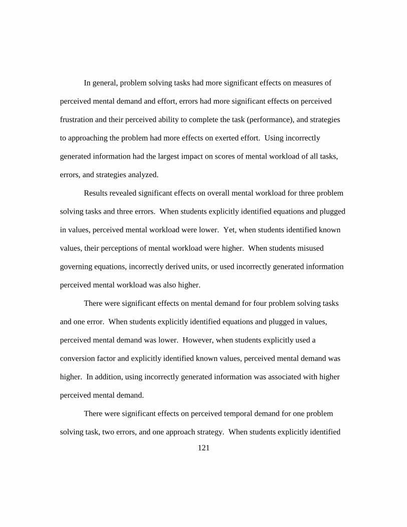
121

In general, problem solving tasks had more significant effects on measures of

perceived mental demand and effort, errors had more significant effects on perceived

frustration and their perceived ability to complete the task (performance), and strategies

to approaching the problem had more effects on exerted effort. Using incorrectly

generated information had the largest impact on scores of mental workload of all tasks,

errors, and strategies analyzed.

Results revealed significant effects on overall mental workload for three problem

solving tasks and three errors. When students explicitly identified equations and plugged

in values, perceived mental workload were lower. Yet, when students identified known

values, their perceptions of mental workload were higher. When students misused

governing equations, incorrectly derived units, or used incorrectly generated information

perceived mental workload was also higher.

There were significant effects on mental demand for four problem solving tasks

and one error. When students explicitly identified equations and plugged in values,

perceived mental demand was lower. However, when students explicitly used a

conversion factor and explicitly identified known values, perceived mental demand was

higher. In addition, using incorrectly generated information was associated with higher

perceived mental demand.

There were significant effects on perceived temporal demand for one problem

solving task, two errors, and one approach strategy. When students explicitly identified

122

known values or used incorrectly generated information, their perception of temporal

demand was higher. When students had inconsistent units, their perception of temporal

demand was lower, as was the case when students utilized a means-ends-analysis

approach strategy.

There were significant effects on performance strain for three errors. When

students incorrectly related variables, had incorrect unknown values, or used incorrectly

generated information, their perceptions of performance strain were higher and thus felt

less confident that they were able to accomplish the task successfully.

There were significant effects on effort for four problem solving tasks and an

approach strategy. When students explicitly identified equations and plugged in values,

their levels of perceived effort were lower. However, when students used conversion

factors or identified known values, their perceptions of perceived effort were higher. In

addition, utilizing a chunking strategy was associated with a lower perceived effort.

Lastly, there were significant effects on perceived frustration for four errors and

one approach strategy. When students misused the governing equation, had an incorrect

calculation, incorrectly derived units, or used incorrectly generated information, their

levels of perceived frustration were higher, as were perceptions of frustration when a plug

and chug strategy was utilized.

123

Identifying performances associated with extreme scores of mental workload

Repeated measures analyses were conducted in order to calculate the significant

effects on mental workload using fixed effects of the problem and the performance

measure under question while accounting for random effects attributed to the student. A

summary of significant effects can be found in Table 7.5 and detailed in Appendix L.

Overall, significant effects were found for seven of the twenty-eight internal process

measures and five of the six outcome measures. Having a correct representation was the

internal process measure with the most impact on mental workload scores while

conceptual errors was the outcome measure with the largest association with mental

workload scores. In most cases, the specific problem was not a significant factor

influencing mental workload, suggesting that these effects are generalizable across

problems.

Results revealed significant effects on overall mental workload for three internal

process measures and three outcome measures. When students had correct representation

and correct equations, their perceived mental workload was lower. Mental workload was

higher when more attempts were necessary to correct mechanical errors. In addition,

mental workload was higher when conceptual errors were present, with higher error rates,

and with attempts that took longer to complete.

Similarly, mental demand was lower when students had correct representations

and higher when a conceptual error was present.

124

Table 7.5: Relationships between performance measures and mental workload

Performance Measures Over

all

Men

tal

Work

load

Men

tal

Dem

and

Tem

pora

l D

eman

d

Per

form

ance

Eff

ort

Fru

stra

tion

Recognize / identify

the problem

# Tries to get correct

unknown

Represent the

problem

Explicit visual

Correct

representation

Organize knowledge

about the problem Correct equation

Allocate resources

(Execution)

# Tries to get correct

mechanical execution

Overprocessing

Monitor progress

toward the goals False alarm rate

Solution Accuracy

Answer Accuracy

Conceptual Errors

Management Errors

Solution efficiency Error Rate

Time to complete

Temporal demand was also alleviated by a correct representation and higher with

conceptual errors as well as management errors, a higher error rate, and a longer time to

complete the problem. Perceived performance strain was related to the most performance

measures. Students who took more tries to overcome incorrect unknown values, those

who erased correct work more often (and related, those with higher false alarm rates)

reported higher performance strain. The same was true for students who committed

125

conceptual errors, management errors, had a higher error rate, and took longer to

complete the problem. In addition, students with more accurate solutions reported lower

performance strain.

Students who utilized more advanced strategies, had correct representations, and

had correct equations, reported perceived effort as lower. Students that committed more

conceptual errors reported perceived effort as higher.

Similar results were shown for students in terms of perceived frustration.

Students who had correct representations and correct equations reported lower perceived

frustration. Students who took more tries to overcome mechanical errors, had more

conceptual errors, and had higher error rates reported higher perceived frustration.

DISCUSSION

The mental workload scores indicated the same distribution of problem difficulty

across problems as the measure of probability of success; however, the subscale measure

of frustration was most highly correlated with problem solving success. It seems

appropriate that either overall mental workload or the subscale of frustration can serve as

potential alternative means of assessing problem difficulty rather than probability of

success. The benefits of using the NASA-TLX as an indicator of problem difficulty is

that it can be used to identify students who feel like they are having trouble completing

the problem and it reveals whether the struggle was due to time pressure or the problem

126

itself. It can alert instructors to negative affective outcomes such as high frustration that

may affect a student’s sense of autonomy. On the other hand, if all the instructor wants

to know is the difficulty of the problem solving task, then simply asking students to rate

how well they were able to accomplish the task (performance) on a scale between failure

and perfection or how frustrated they were with the task will likely be sufficient.

The assessment of problem solving features suggests some methods that can keep

mental workload at optimal levels. Explicit equation identification and subsequently

plugging in values was associated with lower mental workload, which could be used by

novice problem solvers as a way of reducing mental workload if capacity is an issue,

along with utilizing a means-ends-analysis strategy. However, the interpretation of

effects attributed to identifying known values is less clear. Identifying known values was

associated with higher perceived mental workload, which can be explained in two ways.

Either students with lower mental workload capacity identified known values as a way to

reduce mental workload or the process of identifying known values raised metacognitive

awareness of how difficult the task truly was.

Errors should always be avoided and generally were correlated with higher mental

workload. However, the error of inconsistent units was associated with lower temporal

demand, most likely due to the oversimplification of the problem. Similarly, using a

conversion factor was found to be associated with higher mental demand and higher

effort, though these were likely the result of higher metacognitive awareness of the

difficulty of the problem.

127

Similar effects were found for performance measures. Drawing a correct visual

representation and correctly identifying equations are performances associated with lower

mental workload and workload subscales, so the development of these skills should be

emphasized. In addition, certain inefficient performances were strongly associated with

higher mental workload or workload subscales such as requiring multiple attempts before

obtaining the correct unknown value and correct mechanical execution, overprocessing

and higher false alarm rates (which are both indicators of erasing correct work), making

conceptual and management errors, and taking more time to complete the problem.

Ideally, these should be avoided if possible, but often occur when mastery has yet to be

achieved, and are normal outcomes of the learning process.

CONCLUSIONS

The NASA-TLX is an appropriate gauge of problem difficulty as it yields similar

results to other accepted methods, such as the probability of success, while generating

much richer information about what students are (or are not) struggling with. Instructors

and researchers can utilize a student’s self-report NASA-TLX scores as an indicator of

cognitive overload by charting student’s perceived workload scores; flagging students

who report mental workloads larger than one standard deviation above the mean for

additional attention. An example is shown in Figure 7.4.

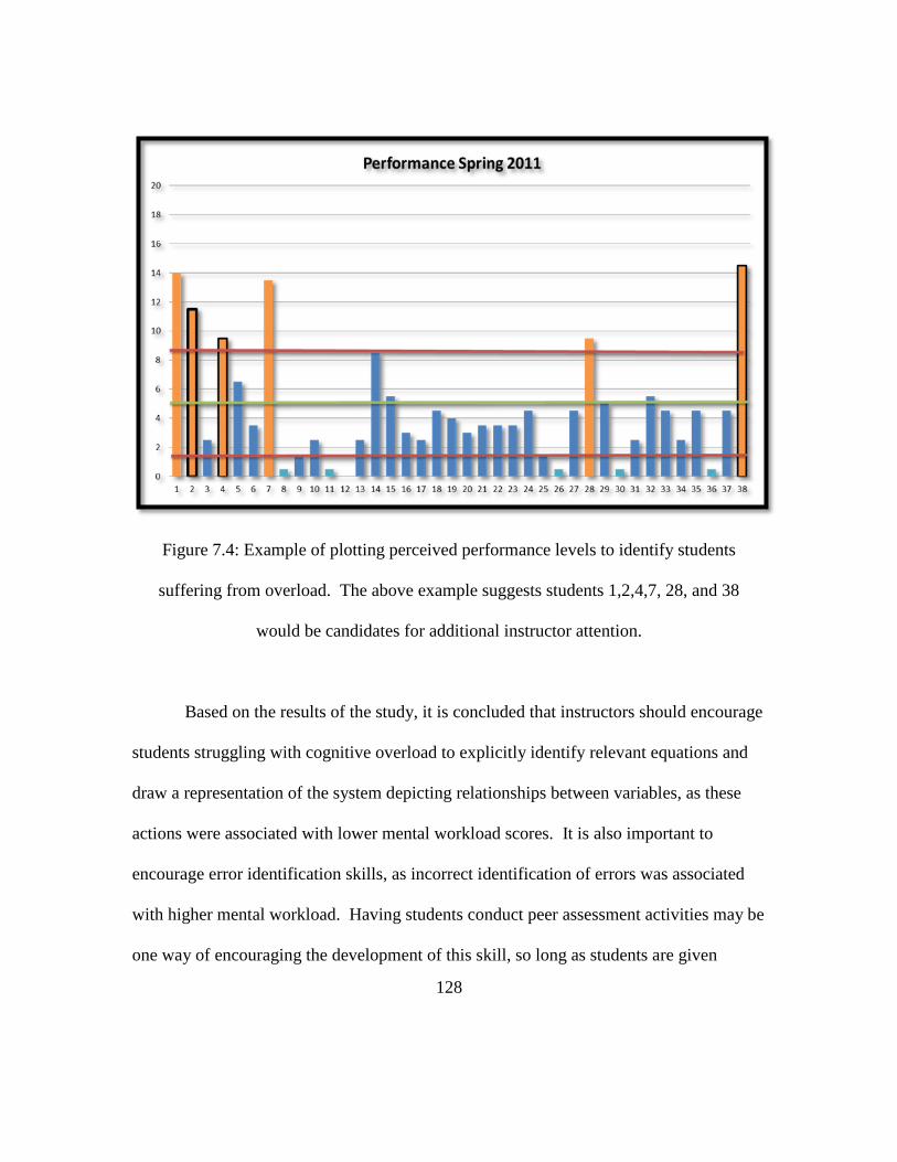
128

Figure 7.4: Example of plotting perceived performance levels to identify students

suffering from overload. The above example suggests students 1,2,4,7, 28, and 38

would be candidates for additional instructor attention.

Based on the results of the study, it is concluded that instructors should encourage

students struggling with cognitive overload to explicitly identify relevant equations and

draw a representation of the system depicting relationships between variables, as these

actions were associated with lower mental workload scores. It is also important to

encourage error identification skills, as incorrect identification of errors was associated

with higher mental workload. Having students conduct peer assessment activities may be

one way of encouraging the development of this skill, so long as students are given

129

feedback on the accuracy of those activities. More research is needed to determine

whether the error identification skills of other students work would transfer to the ability

to self-assess concurrently with problem solving or whether novice students would be

unable to utilize those skills successfully due to other loads on mental workload capacity.

130

CHAPTER EIGHT

HOW DOES STUDENT ACADEMIC PREPARATION INFLUENCE HOW

STUDENTS SOLVE PROBLEM?

A key goal of engineering educators is to identify factors that can limit students’

success in engineering. In first year engineering courses, students possess a wide range

of academic preparation such as their exposure to various mathematics courses and pre-

engineering programs. Additionally, students bring perceptions about their abilities, and

have already begun practicing preferred methods of analysis and documentation.

Understanding how students with different backgrounds develop problem solving skills

in first year engineering programs is of critical importance in order to close achievement

gaps between diverse populations.

This study examines how students solve engineering problems and identifies

variations based on student factors of gender, ethnicity, prior engineering experience, and

mathematics preparation. Solutions for three problems from 27 students were analyzed.

Differences in how students solve problems were assessed based on the prevalence (or

absence) of elements and errors in the problem solving process, which were evaluated

using task analysis.

Results revealed the female students in this study seemed to struggle more than

male students with their problem solving attempts; however, this may be confounded by

the dramatic difference in prior academic preparation. Few effects were found to be

131

related to the ethnicity of the student. Contrary to initial expectations, pre-engineering

experience did not have a significant impact on successfully solving problems; however,

there does appear to be an impact on how students solve problems in terms of both style

and approach. Yet, having completed a calculus course was significantly related to

successful problem solving, and lacking calculus experience was related to an increased

number of errors and a longer completion time. Future research will investigate ways of

overcoming achievement gaps between populations through focused pedagogical

interventions such as through providing feedback on processing errors and inefficiencies.

INTRODUCTION

In view of the one-way migration pattern from engineering majors (Ohland,

Sheppard, Lichenstein, Eris, & Charchra, 2008), it is important to identify factors that

cause students to withdraw from or fail to succeed in engineering courses. Engineering

students from underrepresented populations such as females and minorities have been

shown to have distinctly different engineering education experiences (Adelman, 1998).

Research indicates that males seem to exhibit more advanced problem solving

performances than females (Zhu, 2007) and that females doubt their problem solving

abilities more than males (Felder, Felder, & Mauney, 1995). Research on the

mathematical problem solving of minority students has shown that they suffer a larger

dropout rate from engineering than all other students (National Research Council .

132

Retention Task Force & National Research Council . Committee on Minorities in

Engineering, 1977) and exhibit a lower success rate solving non-routine problems, even

though their solutions indicate proportional skills levels (Malloy & Jones, 1998). Non-

routine problems were those that could be solved with multiple strategies and required

inferential, deductive, or inductive reasoning (Malloy & Jones, 1998). This definition of

non-routing problems describes contextual “story” problems typical of those used in the

first year engineering course under investigation. If this trend is evident in first year

engineering problem solving, it could shed light on a potential factor attributing to the

higher than average withdrawal rate for under-represented minorities. Understanding

how students with different backgrounds develop problem-solving skills in first year

engineering programs is of critical importance in order to close achievement gaps

between diverse populations.

Another potential factor is the level of academic preparation. Engineering

students must apply basic mathematical skills and reasoning to solve problems, ranging

from arithmetic manipulations to analysis of variables. However, the level of mathematic

and engineering preparation they bring to their first-year courses vary widely. Often

instructors find that students do not have the prerequisite knowledge needed or have

strong enough analytical skills to learn new concepts successfully. When students work

through problems, they construct an interpretation of the concepts being taught using pre-

existing knowledge (Bruner, 1973). For meaningful learning to occur, a learner must

make sense out of the information presented and have relevant conceptual knowledge to

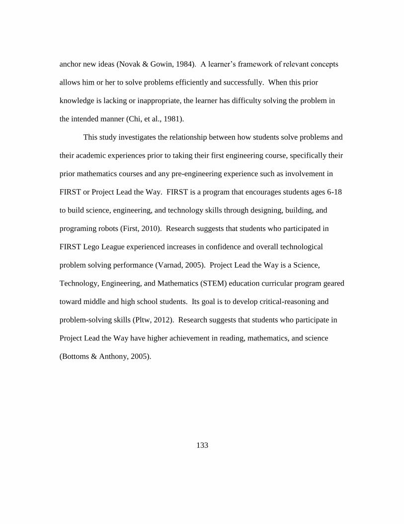
133

anchor new ideas (Novak & Gowin, 1984). A learner’s framework of relevant concepts

allows him or her to solve problems efficiently and successfully. When this prior

knowledge is lacking or inappropriate, the learner has difficulty solving the problem in

the intended manner (Chi, et al., 1981).

This study investigates the relationship between how students solve problems and

their academic experiences prior to taking their first engineering course, specifically their

prior mathematics courses and any pre-engineering experience such as involvement in

FIRST or Project Lead the Way. FIRST is a program that encourages students ages 6-18

to build science, engineering, and technology skills through designing, building, and

programing robots (First, 2010). Research suggests that students who participated in

FIRST Lego League experienced increases in confidence and overall technological

problem solving performance (Varnad, 2005). Project Lead the Way is a Science,

Technology, Engineering, and Mathematics (STEM) education curricular program geared

toward middle and high school students. Its goal is to develop critical-reasoning and

problem-solving skills (Pltw, 2012). Research suggests that students who participate in

Project Lead the Way have higher achievement in reading, mathematics, and science

(Bottoms & Anthony, 2005).

134

METHODS

This research explores relationships between academic preparation and problem

solving features and performance measures. Tablet PCs were used to capture student

problem solving attempts.

Participants and Problems

This study examines problem solving solutions from 27 students enrolled in a first-

year undergraduate engineering course. Three problems were chosen for analysis that

covered a range of topics typical of an introductory engineering course including 1)

efficiency, 2) circuits, and 3) pressure. All problems 1) had a constrained context,

including pre-defined elements (problem inputs), 2) allowed multiple predictable

procedures or algorithms, and 3) had a single correct answer (Jonassen, 2004). All three

problems were story problems, in which the student is presented with a narrative that

embeds the values needed to obtain a final answer (Jonassen, 2010).

Data collection instruments

Students completed a beginning of the semester survey, which asked open ended

responses to questions of a) gender, b) ethnicity, c) participation in any pre-engineering

activities, and d) previous mathematics courses and grades. There were 21 male and 6

female participants. Twenty-three of the participants were Caucasian. Seven of the

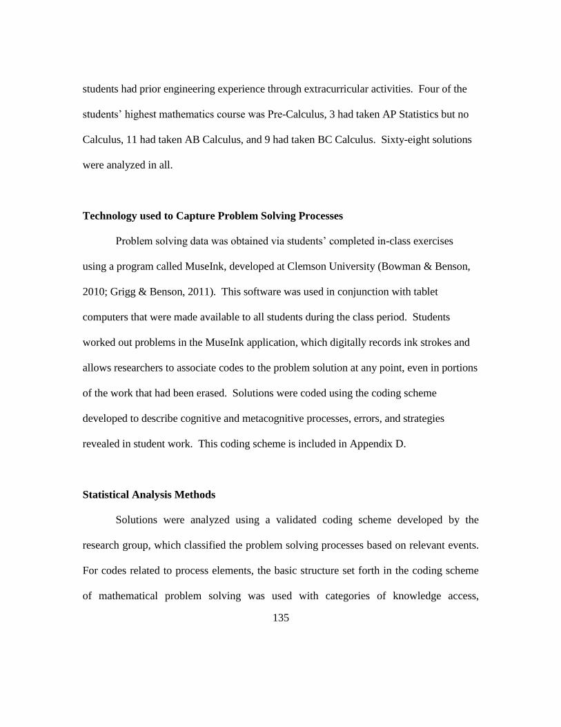
135

students had prior engineering experience through extracurricular activities. Four of the

students’ highest mathematics course was Pre-Calculus, 3 had taken AP Statistics but no

Calculus, 11 had taken AB Calculus, and 9 had taken BC Calculus. Sixty-eight solutions

were analyzed in all.

Technology used to Capture Problem Solving Processes

Problem solving data was obtained via students’ completed in-class exercises

using a program called MuseInk, developed at Clemson University (Bowman & Benson,

2010; Grigg & Benson, 2011). This software was used in conjunction with tablet

computers that were made available to all students during the class period. Students

worked out problems in the MuseInk application, which digitally records ink strokes and

allows researchers to associate codes to the problem solution at any point, even in portions

of the work that had been erased. Solutions were coded using the coding scheme

developed to describe cognitive and metacognitive processes, errors, and strategies

revealed in student work. This coding scheme is included in Appendix D.

Statistical Analysis Methods

Solutions were analyzed using a validated coding scheme developed by the

research group, which classified the problem solving processes based on relevant events.

For codes related to process elements, the basic structure set forth in the coding scheme

of mathematical problem solving was used with categories of knowledge access,

136

knowledge generation, self-management (Wong, et al., 2002). For codes relating to

errors, a structure derived from error detection literature in accounting, was used to

classify errors as conceptual and mechanical errors (Owhoso, et al., 2002; Ramsay, 1994)

with an added classification of management errors to capture errors in metacognitive

processes. Strategy codes were obtained from a subset of strategies that appeared most

applicable to story problems from the compilation described in “Thinking and Problem

Solving” (Nickerson, 1994).

To investigate variations in how students solve problems, statistical analyses were

conducted to assess differences between groups in terms of the presence of problem

solving elements. Statistical analyses were conducted to investigate whether there were

differences in how students solved problems based on participant factors of 1) gender, 2)

ethnicity, 3) pre-engineering experience, or 4) calculus experience. Then, statistical

analyses were conducted to evaluate whether there were differences in terms of problem

solving performance between groups.

Evaluation of the Variations in How Students Solve Problems: As a primary

investigation, Chi Square tests were conducted to test whether differences in proportions

were larger than due to chance. All problem solving features occurring at least once in

the problem solving attempts were classified as occurring, even if the work was later

modified to eliminate its presence in the final solution. Then, odds ratios were calculated

to determine the magnitude of how much more likely solutions completed by a particular

group were to contain a task element, contain an error, or use a strategy. For this

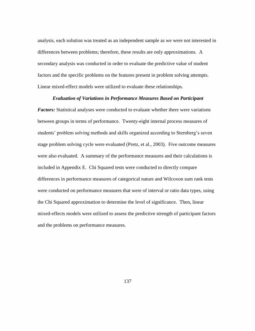
137

analysis, each solution was treated as an independent sample as we were not interested in

differences between problems; therefore, these results are only approximations. A

secondary analysis was conducted in order to evaluate the predictive value of student

factors and the specific problems on the features present in problem solving attempts.

Linear mixed-effect models were utilized to evaluate these relationships.

Evaluation of Variations in Performance Measures Based on Participant

Factors: Statistical analyses were conducted to evaluate whether there were variations

between groups in terms of performance. Twenty-eight internal process measures of

students’ problem solving methods and skills organized according to Sternberg’s seven

stage problem solving cycle were evaluated (Pretz, et al., 2003). Five outcome measures

were also evaluated. A summary of the performance measures and their calculations is

included in Appendix E. Chi Squared tests were conducted to directly compare

differences in performance measures of categorical nature and Wilcoxon sum rank tests

were conducted on performance measures that were of interval or ratio data types, using

the Chi Squared approximation to determine the level of significance. Then, linear

mixed-effects models were utilized to assess the predictive strength of participant factors

and the problems on performance measures.

138

RESULTS

Assessment of problem solving variations by Gender

The level of academic preparation of female students was quite different from that

of male students. Males were more likely to have both pre-engineering experience

(p=0.0004) and calculus experience (p=0.0001). Of the female students in the study, only

33% had calculus experience compared to 86% of male students. Additionally, none of

the female students had pre-engineering experience compared to 33% of male students.

Therefore, it should be noted that differences found in terms of gender are likely due (at

least in part) to differences in level of academic preparation.

Chi squared tests and odds ratios indicated that females were more likely than

males to explicitly write out equations and then plug in values in separate steps (p =

0.042), and had a higher occurrence of incorrectly deriving units (p=0.002). Additionally,

females’ solutions were more likely to indicate the use of lower level strategies such as a

“guess and check strategy”. Results are summarized in Table 8.1 and the complete

assessment of odds ratios is in Appendix M.

In terms of performance assessment, males tended to use higher-level strategies

than females (p=0.005), correctly identify known values (p=0.039), have a lower false

alarm rate (do not erase correct work as often) (p=0.050), and obtained a higher

proportion of accurate final answers (p=0.002). A summary is shown in Table 8.2.

139

Table 8.1: Significant effects of gender based on Chi Squared tests and odds ratios

Process Analysis

Measure

Chi

Square

p

value

Mean

(Male)

Mean

(Female)

Odds Ratio

(Male

more)

Odds Ratio

(Female

more)

Plugged values in

equation 4.13 0.042 0.77 1.00 0.1 9.3

Incorrect unit

derivation 4.52 0.034 0.04 0.20 0.2 6.4

Guess and check 4.18 0.041 0.11 0.33 0.3 3.8

Table 8.2: Performance assessment by gender

Process Analysis Measure Chi

Square p value

Mean

(Male)

Mean

(Female)

Approach Strategy Used 14.36 0.001 0.51 0.20

Number of corrections of mechanical tasks 4.07 0.044 0.08 0.27

Irrelevant information 7.30 0.026 0.17 0.40

Answer Accuracy 11.36 0.001 0.56 0.14

Assessment of Problem Solving Variations by Ethnicity

The level of academic preparation of minority students was roughly equivalent to

that of the remainder of the students. No significant differences were found in terms of

calculus experience (p=0.338) or pre-engineering experience (p=0.999). Of the minority

students in the study, 75% had calculus experience compared to 78% of non-minority

students. Additionally, 25% of minority students had pre-engineering experience

compared to 26% of non-minority students. Therefore, it is reasonable to assume that

differences found based on ethnicity are not attributable to prior academic experiences of

140

participating in a pre-engineering program or completing a calculus class. However, only

a few differences were found that were attributed to ethnicity.

The only significant difference found in terms of problem solving features based

on ethnicity was a larger number of solutions with correct answers but with incorrect

units (p=0.003), as shown in Table 8.3. A complete evaluation of odds ratios is shown in

Appendix N.

Table 8.3: Significant effects of ethnicity based on Chi Squared tests and odds ratios

Process

Analysis

Measure

Chi

Square

p

value Mean

(Caucasians) Mean

(Minorities) Odds Ratios (Caucasians

more )

Odds

Ratios (Minorities

more)

Missing

Units

Throughout

11.95 0.001 0.00 0.20 0.02 45.00

Variation in performances based on ethnicity indicated that the Caucasian

students correctly identified known values more often (p=0.01) and completed the

problems more quickly (p=0.001) as shown in Table 8.4.

Table 8.4: Performance assessment by ethnicity

Process Analysis Measure Chi

Square p value

Mean

(Caucasian)

Mean

(Minority)

Correct known values 6.76 0.01 0.98 0.80

Time to completion 6.57 0.01 14.18 23.69

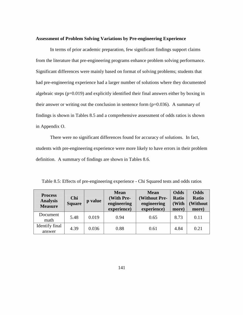
141

Assessment of Problem Solving Variations by Pre-engineering Experience

In terms of prior academic preparation, few significant findings support claims

from the literature that pre-engineering programs enhance problem solving performance.

Significant differences were mainly based on format of solving problems; students that

had pre-engineering experience had a larger number of solutions where they documented

algebraic steps (p=0.019) and explicitly identified their final answers either by boxing in

their answer or writing out the conclusion in sentence form (p=0.036). A summary of

findings is shown in Tables 8.5 and a comprehensive assessment of odds ratios is shown

in Appendix O.

There were no significant differences found for accuracy of solutions. In fact,

students with pre-engineering experience were more likely to have errors in their problem

definition. A summary of findings are shown in Tables 8.6.

Table 8.5: Effects of pre-engineering experience - Chi Squared tests and odds ratios

Process

Analysis

Measure

Chi

Square p value

Mean

(With Pre-

engineering

experience)

Mean

(Without Pre-

engineering

experience)

Odds

Ratio

(With

more)

Odds

Ratio

(Without

more)

Document

math 5.48 0.019 0.94 0.65 8.73 0.11

Identify final

answer 4.39 0.036 0.88 0.61 4.84 0.21

142

Table 8.6: Performance assessment by pre-engineering experience

Process Analysis

Measure

Chi

Square

p

value

Mean (With pre-

engineering

experience)

Mean (Without pre-

engineering

experience)

Correct definition 6.09 0.014 0.76 0.96

Indicate Answer 4.39 0.036 0.88 0.61

Assessment of Problem Solving Variations by Calculus Experience

An extensive set of differences was revealed based on mathematics preparation in

terms of calculus experience, with implications on solution accuracy. Students who had

taken a calculus class had fewer errors in their solutions. Solutions from students without

calculus experience were more likely to solve intermediate values (p=0.048), utilize

labeling or renaming (p = 0.005), use incorrectly generated equations (p =0.048), and

have missing units throughout the entire attempt (p = 0.013). Results are shown in

Tables 8.7 and a complete analysis of odds ratios is included in Appendix P.

Table 8.7: Effects of calculus experience based on Chi Squared tests and odds ratios

Process Analysis

Measure

Chi

Square

p

value

Mean

(With

Calculus

Experience)

Mean

(Without

Calculus

Experience)

Odds

Ratio

(With

more)

Odds

Ratio

(Without

more)

Solve Intermediate value 3.91 0.048 0.80 1.00 0.11 8.86

Labeling / Renaming 7.87 0.005 0.38 0.76 0.18 5.46

Using incorrectly

generated information 3.92 0.048 0.18 0.41 0.31 3.27

Missing units throughout 6.18 0.013 0.00 0.13 0.06 16.61

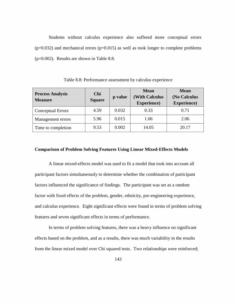
143

Students without calculus experience also suffered more conceptual errors

(p=0.032) and mechanical errors (p=0.015) as well as took longer to complete problems

(p=0.002). Results are shown in Table 8.8.

Table 8.8: Performance assessment by calculus experience

Process Analysis

Measure

Chi

Square p value

Mean

(With Calculus

Experience)

Mean

(No Calculus

Experience)

Conceptual Errors 4.59 0.032 0.33 0.71

Management errors 5.96 0.015 1.06 2.06

Time to completion 9.53 0.002 14.05 20.17

Comparison of Problem Solving Features Using Linear Mixed-Effects Models

A linear mixed-effects model was used to fit a model that took into account all

participant factors simultaneously to determine whether the combination of participant

factors influenced the significance of findings. The participant was set as a random

factor with fixed effects of the problem, gender, ethnicity, pre-engineering experience,

and calculus experience. Eight significant effects were found in terms of problem solving

features and seven significant effects in terms of performance.

In terms of problem solving features, there was a heavy influence on significant

effects based on the problem, and as a results, there was much variability in the results

from the linear mixed model over Chi squared tests. Two relationships were reinforced;

144

those having pre-engineering experience were more likely to identify the final answer and

female students were more likely than males to have incorrect unit derivations. However,

incorrect unit derivations were also associated with being a minority student, having

calculus experience, and lacking pre-engineering experience. Five new but related

effects revealed that those with calculus experience were more likely to explicitly

manipulating equations to solve for variables before plugging in values, students with

pre-engineering experience were more likely to ignore problem constraints, and females

and those with pre-engineering experience were more likely to solve for the wrong

unknown value. In addition, females showed a higher use of the plug-and-chug strategy

while Males who were Caucasian and did not have calculus experience were more likely

to use means-ends-analysis. Results can be found in Appendix Q.

In terms of performance, significant effects were reinforced for six of the eleven

performance measures; however, none of the significant effects associated with calculus

experience remained significant after assessing all participant factors jointly. Females,

Caucasians, and those with pre-engineering experience were more likely to utilize

explicit definition tasks, though students with pre-engineering experience were also more

likely to have incorrect definition tasks (derived from the high occurrence of ignoring

problem constraints). This assessment also reinforced that males used higher-level

strategies to approach the problem, males had higher answer accuracy, those with pre-

engineering experience were more likely to identify the final answer, and minority

students took longer to complete the problems. Correctly identifying known values was

145

related to all participant factors, with males, Caucasians, those with calculus experience

and those without pre-engineering experience obtaining correct known values more often.

Results can be found in Appendix R.

DISCUSSION

This analysis revealed several significant differences in how different students

from this class solved problems. It is important to point out that the findings from this

study many not be generalizable to all classes or even all sections of the particular course

that was investigated. However, other instructors could utilize the methodology

described in this paper as a means of identifying the areas of instructional needs of

students in their own classes. The important thing to take away from this research is that

participant factors do have a profound impact on how students solve problems when they

are allowed to solve problems based on their preferred method, as was the case in this

investigation. It is important to get an initial gauge of student skills so that instruction

can be tailored as appropriate.

That being said, the findings from this investigation do reinforce some of the

findings in past literature on gender and ethnicity differences. This investigation found

evidence of females using lower level strategies (guess-and-check and plug-and-chug)

more often than males. Also, there were few discernible differences in problem solving

abilities based on ethnicity. This investigation did not show a difference based on

146

solution accuracy but there was a significant difference in time to complete the problem,

which could affect success rate if there is a time constraint.

In addition, results from this investigation indicated that problem solving

techniques can be taught, as evidence of more formal problem solving techniques was

evident in work completed by those with pre-engineering experience that were likely

developed in those programs such as documenting math and indicating the final answer.

However, the speed and accuracy of problem solutions were not impacted by pre-

engineering experience. The only negative item associated with pre-engineering

experience was the error of ignoring problem constraints, which in turn reduced the

accuracy of the problem definition. All instances occurred in the second problem, the

equivalent circuit problem. The students may have adopted a slight overconfidence

based on their prior experience and jumped into solving the problem without fully

understanding the constraints of the problem, or it could simply be a fluke. However, it

would be interesting to see if the effect would disappear if the problem was presented in a

more hands-on approach where students were actually given the physical components

available for use in the equivalent circuit.

As predicted, prior math experience was highly correlated with measures of

problem solving success, with evidence of solutions with fewer conceptual and

management errors and faster completion times based on higher levels of mathematics

preparation. Calculus experience was also associated with techniques that are more

efficient such as avoiding tasks such as solving for intermediate values or renaming

147

variables. However, these effects were washed out when all participant factors were

evaluated jointly. It is unlikely that having experienced a calculus class directly affects

these outcomes, as calculus was not needed to solve any of these problems. It is more

likely that the student’s advanced abilities have afforded them the opportunity to

complete a calculus class before entering this class or that practice solving problems from

a higher difficulty math course has helped them develop stronger problem solving skills.

CONCLUSIONS

While the problem solving techniques and resulting performances vary greatly

across incoming students, there is no reason for instructors to remain blind to these

differences. By conducting a performance assessment, instructors can uncover

deficiencies held by individual students or assess the overall skill level of the class in

order to set reasonable expectations. If this evaluation had been conducted at the

beginning of the semester, instructors would have been able to recognize the risk held by

the female students. The instructor could have possibly provided additional guidance to

help them develop skills necessary to achieve problem solving success at a higher rate

than 1/15 as was the case in this assessment.

Results also reveal the importance of knowing that students have the pre-requisite

knowledge required to succeed in the course. It may have been helpful to provide

additional assistance to students who did not have calculus experience before taking the

148

course. A different option would be to group students into peer teams where they can

work together to solve problems, distributing students based on pre-engineering

experience and prior math experience to ensure a diverse team. The number of potential

interventions based on the skills and abilities of students is nearly endless. However, the

purpose of this study is not to postulate on what interventions may be best, but to provide

a framework that will provide means of evaluating potential achievement gaps between

populations. This method may be used by future research to assess the effectiveness of

instructional interventions in reducing achievement gaps.

149

CHAPTER NINE

ENHANCING PROBLEM SOLVING ASSESSMENT WITH

PROCESS CENTERED ANALYSIS

In order to assess the development of skills, it is necessary to be able to assess the

students’ individual performances on a common set of criteria at various points in their

studies. Traditional approaches to grading problem solving solutions only enable the

evaluation of solution accuracy and do not give insight into students’ problem solving

skills levels. The purpose of this research is to establish an evidenced-based method for

assessing problem solutions that can be utilized by researchers and instructors to assess

problems from a variety of contexts using a common assessment.

Performance measures were assessed by evaluating the level of association

between internal process measures and outcome measures using linear mixed-effects

models. This assessment was then used to create two rubrics that can be utilized to assess

student skills levels throughout the problem solving process that are linked to problem

solving success: one for use with recorded solutions and one for use with paper solutions.

While this rubric is based on evaluations of performance from well-defined story

problems, it is projected that these rubrics can also be applied to a wider range of

problem solving tasks.

150

INTRODUCTION

Traditionally, student problem solving performance is assessed based on

outcomes but ultimately the grading criteria is up to the instructor’s judgment, and

everyone has their own opinion (Reeves, 2008). Therefore, grading policies do not

always accurately represent a student’s level of achievement or learning gains. The most

effective grading policies provide accurate, specific, and timely feedback designed to

improve student performance and assign grades based on summative assessment, taking

into account the trend of student achievement across the semester rather than averaging

performances (Marzano & Heflebower, 2011; O'Connor, 2010).

Standards-based assessment is gaining popularity as a means of assessing that a

student has achieved minimum competencies. In this system, students are compared to

benchmarks for what they are expected to know rather than comparing to a norm such as

the class average. Standards based assessments rely heavily on rubrics or scoring guides

to encourage consistency in assessment across performance evaluations (Reeves, 2002).

Effective rubrics 1) include all important elements, 2) include only unidimensional

elements, 3) have ratings that are distinct, comprehensive, and descriptive, and 4)

communicates clearly with learners (Jonassen, 2004). Jonassen suggests a six item rubric

of criteria to evaluate performance of story (word) problems: 1) accuracy of problem

classification, 2) identification of initial conditions, 3) accuracy of equations, 4) accuracy

of answer estimate, 5) unit consistency, and 6) accuracy of answer (Jonassen, 2004). He

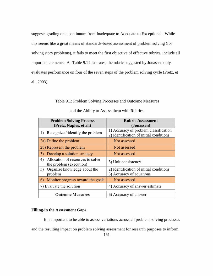
151

suggests grading on a continuum from Inadequate to Adequate to Exceptional. While

this seems like a great means of standards-based assessment of problem solving (for

solving story problems), it fails to meet the first objective of effective rubrics, include all

important elements. As Table 9.1 illustrates, the rubric suggested by Jonassen only

evaluates performance on four of the seven steps of the problem solving cycle (Pretz, et

al., 2003).

Table 9.1: Problem Solving Processes and Outcome Measures

and the Ability to Assess them with Rubrics

Problem Solving Process

(Pretz, Naples, et al.)

Rubric Assessment

(Jonassen)

1) Recognize / identify the problem 1) Accuracy of problem classification

2) Identification of initial conditions

2a) Define the problem Not assessed

2b) Represent the problem Not assessed

3) Develop a solution strategy Not assessed

4) Allocation of resources to solve

the problem (execution) 5) Unit consistency

5) Organize knowledge about the

problem

2) Identification of initial conditions

3) Accuracy of equations

6) Monitor progress toward the goals Not assessed

7) Evaluate the solution 4) Accuracy of answer estimate

Outcome Measures 6) Accuracy of answer

Filling-in the Assessment Gaps

It is important to be able to assess variations across all problem solving processes

and the resulting impact on problem solving assessment for research purposes to inform

152

instructional interventions that could improve awareness of skills deficiencies. If the

only way to assess problem solving attempts was using retrospective analysis of

handwritten paper solutions, a rubric containing assessment of the six items provided by

Jonassen may be the best means of assessment available within the constraints of the

medium. However, when a recording of the entire problems solving process is available

for analysis, as through video recordings or digital Ink (as used in this research effort),

then process analysis can be used to evaluate additional problem solving skills. Process-

based analysis examines methods and systems and looks to identify weak points in the

process (Scheer, 2003) and can also be used to assess efficiency of processes. While this

form of assessment is more labor intensive, the enhanced assessment can uncover skills

deficiencies and has the potential for significant improvement in student learning gains.

MEASURES OF INTERNAL PROCESSES OF THE PROBLEM SOLVING STAGES

Education and human performance literature was utilized to determine measures

that evaluate student performance within the seven stages of Sternberg’s problem solving

cycle. Twenty-eight internal process measures were created and used to evaluate student

problem solving attempts. Table 9.2 describes the breakout of the number of measures

across stages. A list of measures is included in Appendix E.

153

Table 9.2: Number of measures developed to assess problem solving processes

Problem Solving Stage Number of measures

1 Recognize / identify the problem 3

2a

2b

Define the problem

Represent the problem

3

3

3 Develop a solution strategy 1

4 Organize knowledge about the problem 5

5 Allocate resources for solving the problem 8

6 Monitor progress toward the goals 3

7 Evaluate the solution 2

MEASURES OF PERFORMANCE OUTCOMES

Traditionally, instructors simply evaluate students’ solutions based on the

accuracy of the final answer (Szetela, 1987). However, other measures can be used to

further evaluate the solution in terms of solution accuracy as well as process efficiency.

Seven outcome measures were created and used to evaluate the resulting outcomes of

student problem solving attempts. Table 9.3 describes the breakout of the outcome

measures. Solution accuracy was assessed based on measures of success (100% correct

solution), level of accuracy (average level of accuracy, taking into account partial credit

for having correct answers with incorrect units and multi-part problems with incorrect

answers for some parts), and three measures of different types of errors. Attempt

efficiency was assessed based on error rate and time to completion.

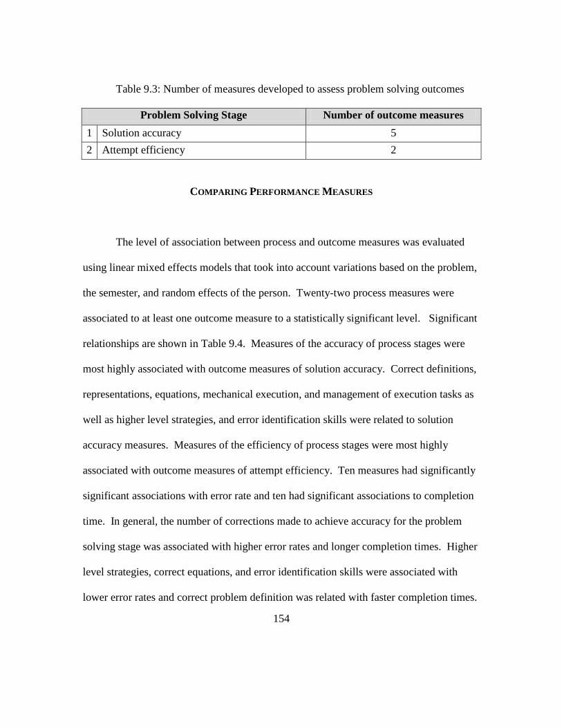
154

Table 9.3: Number of measures developed to assess problem solving outcomes

Problem Solving Stage Number of outcome measures

1 Solution accuracy 5

2 Attempt efficiency 2

COMPARING PERFORMANCE MEASURES

The level of association between process and outcome measures was evaluated

using linear mixed effects models that took into account variations based on the problem,

the semester, and random effects of the person. Twenty-two process measures were

associated to at least one outcome measure to a statistically significant level. Significant

relationships are shown in Table 9.4. Measures of the accuracy of process stages were

most highly associated with outcome measures of solution accuracy. Correct definitions,

representations, equations, mechanical execution, and management of execution tasks as

well as higher level strategies, and error identification skills were related to solution

accuracy measures. Measures of the efficiency of process stages were most highly

associated with outcome measures of attempt efficiency. Ten measures had significantly

significant associations with error rate and ten had significant associations to completion

time. In general, the number of corrections made to achieve accuracy for the problem

solving stage was associated with higher error rates and longer completion times. Higher

level strategies, correct equations, and error identification skills were associated with

lower error rates and correct problem definition was related with faster completion times.

155

Table 9.4: Associations between process measures and outcome measures

Performance Measures

Su

cces

s

An

swer

Acc

ura

cy

Co

nce

ptu

al E

rro

rs

Mec

han

ical

Err

ors

Man

agem

ent

Err

ors

Err

or

Rat

e

Tim

e to

com

ple

te

Recognize / identify

the problem 1B Correct unknown

Define the problem 2B Correct definition

Represent the

problem

2D Explicit visual

2E Correct representation

2F Number of Corrections to

representation

Develop a solution

strategy 3 Strategy

Organize knowledge

about the problem

4A Explicit info

4B Correct known values

4C Correct equation

4D Number of Corrections to

known values

Allocate resources

(Execution)

5A Execute task

5B Correct mechanical

5C Number of Corrections

Mechanical

5D Correct management

5E Number of Corrections

Management

5F Number of tasks

5G Erasing correct work

5H Irrelevant Info

Monitor progress

toward the goals

6A Sensitivity

6B Hit Rate

6C False Alarm Rate

156

Detailed descriptions of linear mixed-effects models can be seen in Appendix S.

Measures from Stage 1: Recognize / Identify the problem did not have significant effects

on problem solving success; however, it is likely this is due to the problems being well-

defined and including specifically what to solve for. It is projected that in problems that

are more ill-defined, measures of this stage would have been more highly associated with

outcome measures. There were also no significant effects found for Stage 7: Evaluate the

solution, though the sample of students explicitly completing these tasks on their own

was so small that the effects could not be evaluated from this sample of solutions.

Therefore, it is suggested to retain these measures in the proposed rubric and to be

reassessed by future research efforts.

CREATION OF A PROBLEM SOLVING PROCESS RUBRIC

Based on the results of the analysis, an evidence-based rubric was created to

assess performance, adjusting scales so that they are summative to problem solving

success. The complete rubric of all process measures can be found in Appendix U. The

use of this rubric has implication for both research and instructional purposes. This

rubric will allow researchers to investigate the effectiveness of various pedagogical

interventions in terms of improving problem solving performance and pinpoint the

process that was most impacted. It also enables instructors to identify skills deficiencies

in students’ work and target instructional interventions more effectively.

157

The major advantage to this rubric over traditional grading methods is that it can

be utilized as a personalized feedback system to inform students of their level of

proficiency as well as pinpoint deficiencies. This information could then be utilized by

instructors to route students to resources for overcoming these problems or other

instructional interventions.

One difficulty with using the extended process analysis rubric is that recordings of

the problem solutions are required for complete use. If researchers or instructors do not

have access to a program such as MuseInk, they can still utilize an abbreviated version of

the process analysis, but efficiency measures cannot be assessed and process stages 3 and

6, developing a solution strategy and monitoring progress, cannot be adequately assessed

without a recorded solution. However, it is possible to utilize a similar rubric for hand

written problems that evaluate the problem solution in terms of five of the seven problem

solving processes (six of the eight with define and represent the problem are viewed as

separate stages) and solution accuracy. The paper version of this abbreviated rubric is

shown in Table 9.5 and a screenshot of the database version is shown in Table 9.6. This

version of the rubric is more practical for use by instructors or researchers who do not

have access to problem recording resources. One challenge that comes from this

restricted assessment is how to increase awareness of the two problem solving processes

that cannot be evaluated, developing a solution strategy and monitoring progress, as

performance in these processes were among the most highly correlated with success.

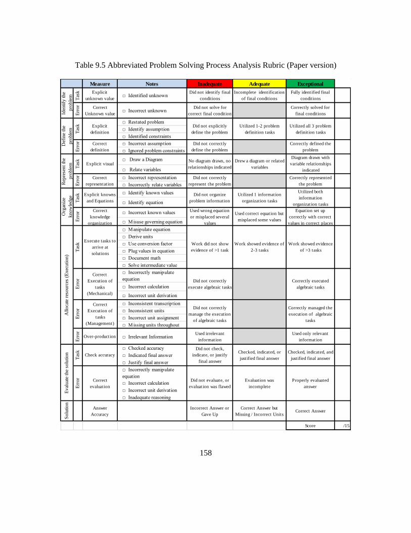
158

Table 9.5 Abbreviated Problem Solving Process Analysis Rubric (Paper version)

Measure Notes Inadequate Adequate Exceptional

Tas

k Explicit

unknown value□ Identified unknown

Did not identify final

conditions

Incomplete identification

of final conditions

Fully identified final

conditions

Err

or Correct

Unknown value□ Incorrect unknown

Did not solve for

correct final condition

Correctly solved for

final conditions

□ Restated problem

□ Identify assumption

□ Identified constraints

□ Incorrect assumption

□ Ignored problem constraints

□ Draw a Diagram

□ Relate variables

□ Incorrect representation

□ Incorrectly relate variables

□ Identify known values

□ Identify equation

□ Incorrect known values

□ Misuse governing equation

□ Manipulate equation

□ Derive units

□ Use conversion factor

□ Plug values in equation

□ Document math

□ Solve intermediate value

□ Incorrectly manipulate

equation

□ Incorrect calculation

□ Incorrect unit derivation

□ Inconsistent transcription

□ Inconsistent units

□ Incorrect unit assignment

□ Missing units throughout

Err

or

Over-production □ Irrelevant InformationUsed irrelevant

information

Used only relevant

information

□ Checked accuracy

□ Indicated final answer

□ Justify final answer

□ Incorrectly manipulate

equation

□ Incorrect calculation

□ Incorrect unit derivation

□ Inadequate reasoning

So

luti

on

Answer

Accuracy

Incorrect Answer or

Gave Up

Correct Answer but

Missing / Incorrect UnitsCorrect Answer

Score /15

Correct

evaluation

Did not evaluate, or

evaluation was flawed

Evaluation was

incomplete

Properly evaluated

answer

Correctly managed the

execution of algebraic

tasks

Ev

alu

ate

the

solu

tio

n

Tas

k

Check accuracy

Did not check,

indicate, or justify

final answer

Checked, indicated, or

justified final answer

Checked, indicated, and

justified final answer

Err

or

Err

or

Correct

Execution of

tasks

(Mechanical)

Did not correctly

execute algebraic tasks

Correctly executed

algebraic tasks

All

oca

te r

eso

urc

es (

Ex

ecu

tio

n)

Tas

k

Execute tasks to

arrive at

solutions

Work did not show

evidence of >1 task

Work showed evidence of

2-3 tasks

Work showed evidence

of >3 tasks

Err

or

Correct

Execution of

tasks

(Management)

Did not correctly

manage the execution

of algebraic tasks

Err

or Correct

knowledge

organization

Used wrong equation

or misplaced several

values

Used correct equation but

misplaced some values

Equation set up

correctly with correct

values in correct places

Org

aniz

e

kn

ow

led

ge

Tas

k Explicit knowns

and Equations

Did not organize

problem information

Utilized 1 information

organization tasks

Utilized both

information

organization tasks

Err

or Correct

representation

Did not correctly

represent the problem

Correctly represented

the problem Rep

rese

nt

the

pro

ble

m Tas

k

Explicit visual No diagram drawn, no

relationships indicated

Drew a diagram or related

variables

Diagram drawn with

variable relationships

indicated

Utilized all 3 problem

definition tasks

Err

or Correct

definition

Did not correctly

define the problem

Correctly defined the

problem

Iden

tify

th

e

pro

ble

m

Def

ine

the

pro

ble

m Tas

k Explicit

definition

Did not explicitly

define the problem

Utilized 1-2 problem

definition tasks

159

Table 9.6 Abbreviated Problem Solving Process Analysis Rubric (Database version)

160

IMPLICATIONS FOR PRACTICE

This research investigation revealed several opportunities to advance educational

practice in order to promote the growth of strong problem solvers. While the results have

only been evaluated in the first year engineering classroom, the techniques are likely

extendable to other related areas such as science, technology, or mathematics courses and

even non-stem courses and could likely be included in secondary education classes.

Evidence suggests that instructors can promote positive outcomes by encouraging

students to utilize planning and visualization tasks, specifically encouraging students to

spend time explicitly documenting and checking the accuracy of 1) the unknown value,

2) the known values, 3) the relevant equations, and 4) a schematic visualization of the

system (a diagram illustrating the relationships between variables). However, simply

requiring the use of these activities is not completely effective, and students may not fully

adopt the behaviors as intended unless they understand how they benefit from their use.

The research also provided methods that can be utilized by instructors to identify

students who could benefit from personalized instruction. One is to have students self-

rate their perceived level of difficulty as with the NASA-TLX survey and identify

students that express extremely high ratings of mental workload. A second is to utilize

the abbreviated rubric to evaluate the problem solving process and identify students with

multiple scores that fall in the inadequate range or an overall score that is low (such as

0 -5 on a 15 point scale).

161

IMPLICATIONS FOR FUTURE RESEARCH

The results from this research suggested several potential instructional

interventions that could potentially be used to aid din the development of problem

solving skills. Evaluating the effectiveness of these instructional techniques will be the

focus of future research initiatives. Using the extended rubric, researchers can evaluate

the variation of performances of specific problem solving processes, comparing student

problem solving attempts from the intervention group and a control group where no

intervention was implemented.

One currently ongoing research effort is looking at evaluating the effectiveness of

implicitly training the problem solving process using guided solutions. Two types of

problems were created based on the National Academy of Engineering’s Grand

Challenge of providing access to clean water. Both problems are designed to encourage

students to progress through the problem solving cycle, with parts of the solution asking

students to conceptualize the system, execute calculations, and reflect on the

interpretation of results. The effectiveness of this pedagogical intervention will be

evaluated to determine whether this type of problem structure promotes heightened

problem solving performance.

In the future, this research will be utilized in a module designed to explicitly teach

students problem solving skills. The rubric will be used to provide feedback to students.

In the same effort, student’s perceptions of the form of feedback will be assessed.

162

Additionally, instructional activities will be designed that focus on addressing

problem solving tasks and showed the biggest performance disparities across populations

in attempts to “level the playing field” of entering students. Specifically these include 1)

translating information from the problem statement into an understanding of the problem,

2) accurate unit derivation, and 3) utilizing strategies to approaching the problem that are

more advanced than plug and chug or guess and check approaches.

Other researchers are encouraged to test the generalizability of this problem

solving assessment method by utilizing it to assess performance in other disciplines or for

other types of problems such as ill-defined project based problems.

163

APPENDICES

164

APPENDIX A

SOLAR EFFICIENCY PROBLEM

One problem with solar energy is that any given point on the planet is illuminated by the

sun for only half of the time at best. It would be helpful, therefore, if there was a simple,

affordable, and efficient means for storing any excess energy generated on sunny days for

use during the night, or on cloudy days.

You are investigating the electrodes used in electrolysis cells as part of a three-stage

process for solar energy collection and storage.

1. Convert sunlight to electricity with photovoltaic cells.

2. Use the electricity generated in an electrolysis cell to split water into its component

elements, hydrogen, and oxygen. The hydrogen can be stored indefinitely. The

oxygen can simply be released into the atmosphere.

3. Use a fuel cell to recombine the stored hydrogen with oxygen from the atmosphere to

generate electricity.

You have obtained an array of new high efficiency thin film photovoltaic cells with an

efficiency of 41%. The efficiency of fuel cells varies with the current demands placed on

them, but the cells you have obtained yield an overall efficiency of 37% at the anticipated

load.

Assume the total solar power on the solar cells is 2000 watts. You conduct four

experiments, each with a different alloy of palladium, platinum, gold, copper, and/or

silver for the electrodes in the electrolysis cell. The final output power from the fuel cell

is measured for each case, and the results are tabulated below. Determine the efficiency

of each electrolysis cell and complete the table.

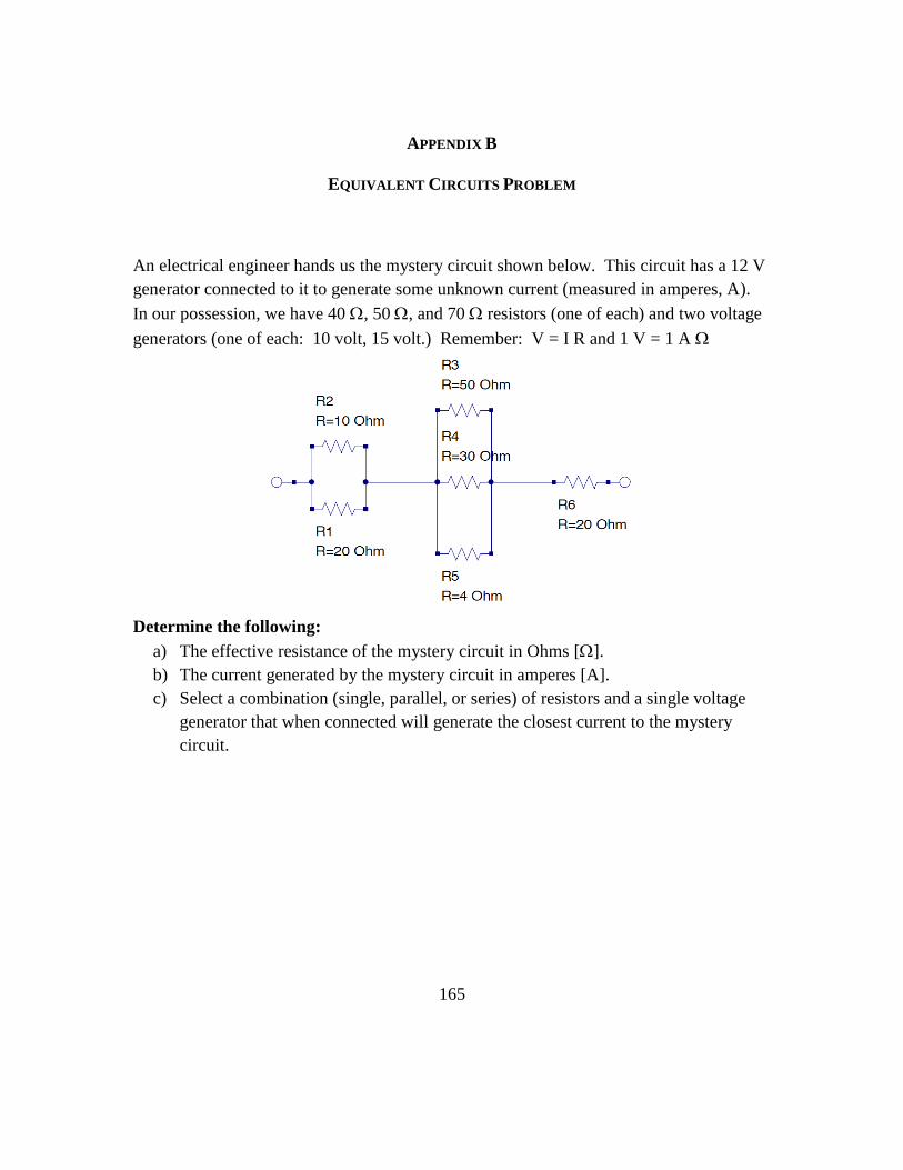
165

APPENDIX B

EQUIVALENT CIRCUITS PROBLEM

An electrical engineer hands us the mystery circuit shown below. This circuit has a 12 V

generator connected to it to generate some unknown current (measured in amperes, A).

In our possession, we have 40 , 50 , and 70 resistors (one of each) and two voltage

generators (one of each: 10 volt, 15 volt.) Remember: V = I R and 1 V = 1 A

Determine the following:

a) The effective resistance of the mystery circuit in Ohms [].

b) The current generated by the mystery circuit in amperes [A].

c) Select a combination (single, parallel, or series) of resistors and a single voltage

generator that when connected will generate the closest current to the mystery

circuit.

166

APPENDIX C

HYDROSTATIC PRESSURE PROBLEMS

ORIGINAL PRESSURE PROBLEM (FALL 2009):

A cylindrical tank filled to a height of 25 feet with tribromoethylene has been pressurized

to 2 atmospheres (Psurface = 2 atmospheres). The total pressure in at the bottom of the tank

is 4 atmospheres. Determine the density of tribromoethylene in units of kilograms per

cubic meter.

SHOW ALL OF YOUR WORK. If you do any calculations, write the calculation out

in MuseInk.

ALTERNATIVE PRESSURE PROBLEM (SPRING 2011):

A cylindrical tank filled with acetic acid (vinegar) has been pressurized to 3 atmospheres

(Psurface = 3 atmospheres) for processing. The total pressure at the bottom of the tank is 5

atmospheres. If the density of acetic acid is 1.01 grams per milliliter, determine the

height of the liquid in the tank in units of feet.

SHOW ALL OF YOUR WORK. If you do any calculations, write the calculation out

in MuseInk.

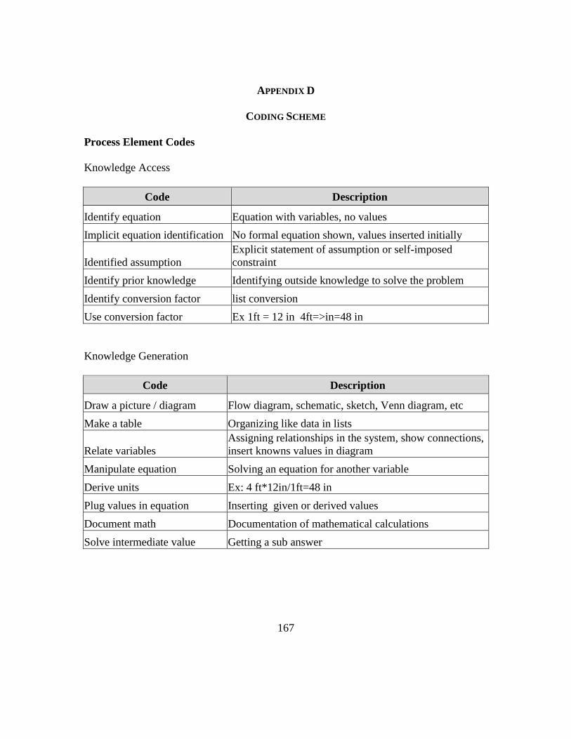
167

APPENDIX D

CODING SCHEME

Process Element Codes

Knowledge Access

Code Description

Identify equation Equation with variables, no values

Implicit equation identification No formal equation shown, values inserted initially

Identified assumption

Explicit statement of assumption or self-imposed

constraint

Identify prior knowledge Identifying outside knowledge to solve the problem

Identify conversion factor list conversion

Use conversion factor Ex 1ft = 12 in 4ft=>in=48 in

Knowledge Generation

Code Description

Draw a picture / diagram Flow diagram, schematic, sketch, Venn diagram, etc

Make a table Organizing like data in lists

Relate variables

Assigning relationships in the system, show connections,

insert knowns values in diagram

Manipulate equation Solving an equation for another variable

Derive units Ex: 4 ft*12in/1ft=48 in

Plug values in equation Inserting given or derived values

Document math Documentation of mathematical calculations

Solve intermediate value Getting a sub answer

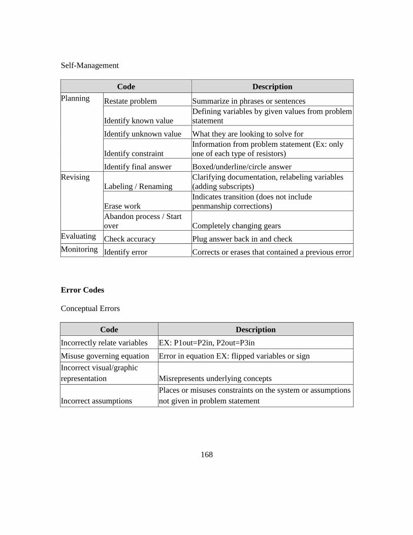
168

Self-Management

Code Description

Planning Restate problem Summarize in phrases or sentences

Identify known value

Defining variables by given values from problem

statement

Identify unknown value What they are looking to solve for

Identify constraint

Information from problem statement (Ex: only

one of each type of resistors)

Identify final answer Boxed/underline/circle answer

Revising

Labeling / Renaming

Clarifying documentation, relabeling variables

(adding subscripts)

Erase work

Indicates transition (does not include

penmanship corrections)

Abandon process / Start

over Completely changing gears

Evaluating Check accuracy Plug answer back in and check

Monitoring Identify error Corrects or erases that contained a previous error

Error Codes

Conceptual Errors

Code Description

Incorrectly relate variables EX: P1out=P2in, P2out=P3in

Misuse governing equation Error in equation EX: flipped variables or sign

Incorrect visual/graphic

representation Misrepresents underlying concepts

Incorrect assumptions

Places or misuses constraints on the system or assumptions

not given in problem statement

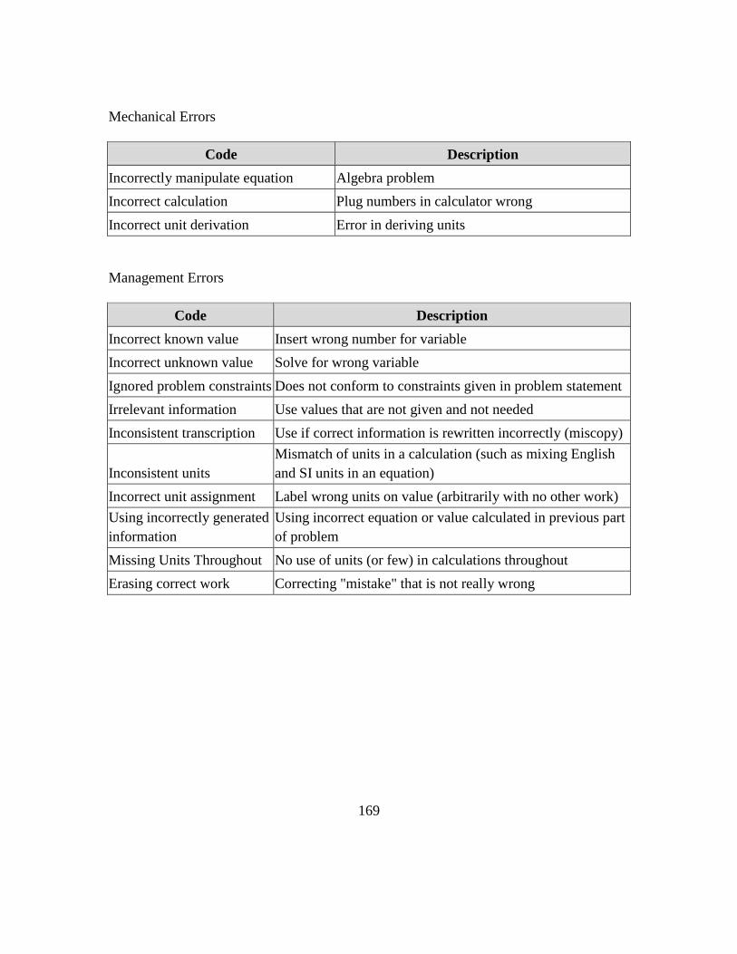
169

Mechanical Errors

Code Description

Incorrectly manipulate equation Algebra problem

Incorrect calculation Plug numbers in calculator wrong

Incorrect unit derivation Error in deriving units

Management Errors

Code Description

Incorrect known value Insert wrong number for variable

Incorrect unknown value Solve for wrong variable

Ignored problem constraints Does not conform to constraints given in problem statement

Irrelevant information Use values that are not given and not needed

Inconsistent transcription Use if correct information is rewritten incorrectly (miscopy)

Inconsistent units

Mismatch of units in a calculation (such as mixing English

and SI units in an equation)

Incorrect unit assignment Label wrong units on value (arbitrarily with no other work)

Using incorrectly generated

information

Using incorrect equation or value calculated in previous part

of problem

Missing Units Throughout No use of units (or few) in calculations throughout

Erasing correct work Correcting "mistake" that is not really wrong

170

Approach Strategy Codes

Code Description

Plug and chug Plug numbers into equations without understanding why

Guess and Check Try values and see what gives good answers

Work Backwards Choose steps based on known solution

Utilize a similar

problem Refer to or work from book example

Segmentation

Discovering or acknowledging multiple parts to problem. Aka

problem decomposition or subgoaling

Chunking Collapsing multiple parts into one step

Means-end analysis Work to minimize differences between goal and starting point

Forward chaining Planning out path to solve problem

Specialization/Extr

eme cases Considering abstract or extreme forms of problem

Solution Accuracy Codes

Code Description

Correct Answer Correctly calculated final answer

Correct but Missing/Incorrect Units Correct value with no or incorrect units

Incorrect Answer Solved for wrong variable, skipped steps

Gave up Failed to produce an answer

171

APPENDIX E

INTERNAL PROCESS MEASURES AND CALCULATIONS

Problem

Solving Stage

Internal Process

Measures Calculation

1

Recognize /

identify the

problem

Explicit

unknown value Completed IIf(Identify unknowns>0,1,0)

Correct

Unknown value Accuracy IIf(Count([Incorrect unknown value]>0,0,1)

# Tries to get

correct unknown Efficiency

IIf(Count([Incorrect unknown value]>0, “NA”,

Count([Incorrect unknown value-HIT]))

2a Define the

problem

Explicit

definition Completed

Sum(IIf(Count([Restate problem]>0,1,0)) +

IIf(Count([Identify assumption]>0,1,0))+

IIf(Count([Identify constraint]>0,1,0)))

Correct

definition Accuracy

IIf(Count([Incorrect constraint]>0,0,

IIf(Count([Incorrect assumption]>0,0,1) )

# Tries to get

correct

definition

Efficiency

IIf(Count([Incorrect constraint]>0, “NA”,

IIf(Count([Incorrect assumption]>0, “NA”,

Sum(Count([Incorrect constraint -HIT])+

Count([Incorrect assumption -HIT])))

2b

Represent

the

problem

Explicit visual Completed IIf([Draw a picture / diagram]>0,

IIf([Relate variables]>0, 1,0.5),0)

Correct

representation Accuracy

IIf(([Draw a picture/diagram]+[Relate variables])>0,

IIf(([Incorrect visual/graphic representation] +

[Incorrectly relate variables])>0,0,1),0)

# Tries to get

correct

representation

Efficiency

IIf(Count([Incorrect visual representation]>0, “NA”,

IIf(Count([Incorrectly relate variables]>0, “NA”,

Sum(Count([Incorrect visual representation-HIT])+

Count([Incorrectly relate variables -HIT])))

3

Develop a

solution

strategy

Approach

Strategy Used Efficiency

IIf([Plug and chug], 0, IIf([Guess and check], 0,

IIf([Segmentation],0.5, IIf([Means end analysis],0.5,

IIf([Chunking],1, IIf([Forward chaining],1, “other”)))

4

Organize

knowledge

about the

problem

Explicit knowns

and Equations Completed

Sum(IIf(Count([Identify known values]>0,1,0)) +

IIf(Count([Identify equation]>0,1,0)))

Correct knowns Accuracy IIf(Count([Incorrect known value]>0,0,1)

Correct

equation Accuracy IIf(Count([Misuse governing equation]>0,0,1)

# Tries to get

correct knowns Efficiency

IIf(Count([Incorrect known value]>0, “NA”,

Count([Incorrect known value-HIT]))

# Tries to get

correct equation Efficiency

IIf(Count([Misuse equation]>0, “NA”,

Count([Misuse equation -HIT]))

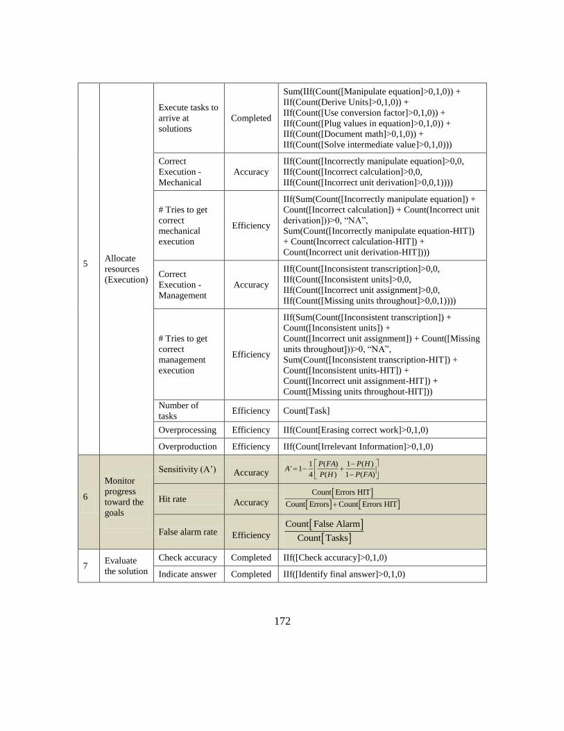
172

5

Allocate

resources

(Execution)

Execute tasks to

arrive at

solutions

Completed

Sum(IIf(Count([Manipulate equation]>0,1,0)) +

IIf(Count(Derive Units]>0,1,0)) +

IIf(Count([Use conversion factor]>0,1,0)) +

IIf(Count([Plug values in equation]>0,1,0)) +

IIf(Count([Document math]>0,1,0)) +

IIf(Count([Solve intermediate value]>0,1,0)))

Correct

Execution -

Mechanical

Accuracy

IIf(Count([Incorrectly manipulate equation]>0,0,

IIf(Count([Incorrect calculation]>0,0,

IIf(Count([Incorrect unit derivation]>0,0,1))))

# Tries to get

correct

mechanical

execution

Efficiency

IIf(Sum(Count([Incorrectly manipulate equation]) +

Count([Incorrect calculation]) + Count(Incorrect unit

derivation]))>0, “NA”,

Sum(Count([Incorrectly manipulate equation-HIT])

+ Count(Incorrect calculation-HIT]) +

Count(Incorrect unit derivation-HIT])))

Correct

Execution -

Management

Accuracy

IIf(Count([Inconsistent transcription]>0,0,

IIf(Count([Inconsistent units]>0,0,

IIf(Count([Incorrect unit assignment]>0,0,

IIf(Count([Missing units throughout]>0,0,1))))

# Tries to get

correct

management

execution

Efficiency

IIf(Sum(Count([Inconsistent transcription]) +

Count([Inconsistent units]) +

Count([Incorrect unit assignment]) + Count([Missing

units throughout]))>0, “NA”,

Sum(Count([Inconsistent transcription-HIT]) +

Count([Inconsistent units-HIT]) +

Count([Incorrect unit assignment-HIT]) +

Count([Missing units throughout-HIT]))

Number of

tasks Efficiency Count[Task]

Overprocessing Efficiency IIf(Count[Erasing correct work]>0,1,0)

Overproduction Efficiency IIf(Count[Irrelevant Information]>0,1,0)

6

Monitor

progress

toward the

goals

Sensitivity (A’) Accuracy 1 ( ) 1 ( )

' 14 ( ) 1 ( )

P FA P HA

P H P FA

Hit rate Accuracy

Count Errors HIT

 Count Errors Count Errors HIT

False alarm rate Efficiency

Count False Alarm

Count Tasks

7 Evaluate

the solution

Check accuracy Completed IIf([Check accuracy]>0,1,0)

Indicate answer Completed IIf([Identify final answer]>0,1,0)

173

APPENDIX F

OUTCOME MEASURES AND CALCULATIONS

Problem Solving

Outcome Under

Assessment

Performance

Measures Calculation

1

Solution

Accuracy

(Product)

Answer

Accuracy * Average [Answer State]

Conceptual

Errors Count[Conceptual Errors (not corrected)]

Mechanical

Errors Count[Mechanical Errors (not corrected)]

Management

Errors Count[Management Errors (not corrected)]

2

Solution

Efficiency

(Process)

Error Rate

Count Errors

Count Tasks

Time to

complete [End time]-[Start time]

3

Stress

Measures

(Person)

NASA-TLX (5) Sum([Mental Demand]+[Temporal

Demand]+[Performance]+[Effort]+[Frustration])

Mental Demand [0,20] (Self-report)

Temporal

Demand [0,20] (Self-report)

Performance [0,20] (Self-report)

Effort [0,20] (Self-report)

Frustration [0,20] (Self-report)

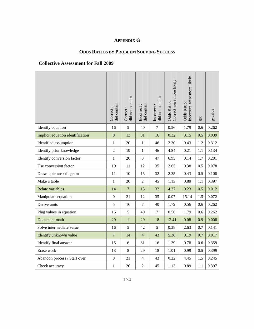
174

APPENDIX G

ODDS RATIOS BY PROBLEM SOLVING SUCCESS

Collective Assessment for Fall 2009

Co

rrec

t :

did

co

nta

in

Co

rrec

t :

did

no

t co

nta

in

Inco

rrec

t :

did

co

nta

in

Inco

rrec

t :

did

no

t co

nta

in

Od

ds

Rat

io:

Co

rrec

t w

ere

mo

re l

ikel

y

Od

ds

Rat

io:

Inco

rrec

t w

ere

more

lik

ely

SE

p-v

alu

e

Identify equation 16 5 40 7 0.56 1.79 0.6 0.262

Implicit equation identification 8 13 31 16 0.32 3.15 0.5 0.039

Identified assumption 1 20 1 46 2.30 0.43 1.2 0.312

Identify prior knowledge 2 19 1 46 4.84 0.21 1.1 0.134

Identify conversion factor 1 20 0 47 6.95 0.14 1.7 0.201

Use conversion factor 10 11 12 35 2.65 0.38 0.5 0.078

Draw a picture / diagram 11 10 15 32 2.35 0.43 0.5 0.108

Make a table 1 20 2 45 1.13 0.89 1.1 0.397

Relate variables 14 7 15 32 4.27 0.23 0.5 0.012

Manipulate equation 0 21 12 35 0.07 15.14 1.5 0.072

Derive units 5 16 7 40 1.79 0.56 0.6 0.262

Plug values in equation 16 5 40 7 0.56 1.79 0.6 0.262

Document math 20 1 29 18 12.41 0.08 0.9 0.008

Solve intermediate value 16 5 42 5 0.38 2.63 0.7 0.141

Identify unknown value 7 14 4 43 5.38 0.19 0.7 0.017

Identify final answer 15 6 31 16 1.29 0.78 0.6 0.359

Erase work 13 8 29 18 1.01 0.99 0.5 0.399

Abandon process / Start over 0 21 4 43 0.22 4.45 1.5 0.245

Check accuracy 1 20 2 45 1.13 0.89 1.1 0.397

175

Identify errors 16 5 45 2 0.14 7.03 0.8 0.023

Incorrectly relate variables 6 15 16 31 0.78 1.29 0.6 0.359

Misuse governing equation 4 17 13 34 0.62 1.63 0.6 0.293

Incorrect visual/graphic representation 0 21 1 46 0.72 1.39 1.7 0.391

Incorrect assumptions 0 21 1 46 0.72 1.39 1.7 0.391

Incorrectly manipulate equation 0 21 1 46 0.72 1.39 1.7 0.391

Incorrect calculation 1 20 9 38 0.21 4.74 0.9 0.096

Incorrect unit derivation 1 20 4 43 0.54 1.86 1.0 0.326

Incorrect known value 3 18 5 42 1.40 0.71 0.7 0.360

Incorrect unknown value 1 20 4 43 0.54 1.86 1.0 0.326

Ignored problem constraints 0 21 8 39 0.11 9.25 1.5 0.129

Irrelevant information 4 17 9 38 0.99 1.01 0.6 0.399

Inconsistent transcription 1 20 5 42 0.42 2.38 1.0 0.265

Inconsistent units 7 14 11 36 1.64 0.61 0.6 0.272

Incorrect unit assignment 2 19 3 44 1.54 0.65 0.9 0.352

Using incorrectly generated information 1 20 15 32 0.11 9.38 0.9 0.018

Missing Units Throughout 1 20 1 46 2.30 0.43 1.2 0.312

Erasing correct work 7 14 15 32 1.07 0.94 0.5 0.396

Plug and chug 1 20 18 29 0.08 12.41 0.9 0.008

Guess and Check 0 21 11 36 0.07 13.55 1.5 0.083

Segmentation 8 13 13 34 1.61 0.62 0.5 0.272

Means-end analysis 7 14 2 45 11.25 0.09 0.8 0.004

Chunking 3 18 14 33 0.39 2.55 0.7 0.147

Forward chaining 3 18 6 41 1.14 0.88 0.7 0.392

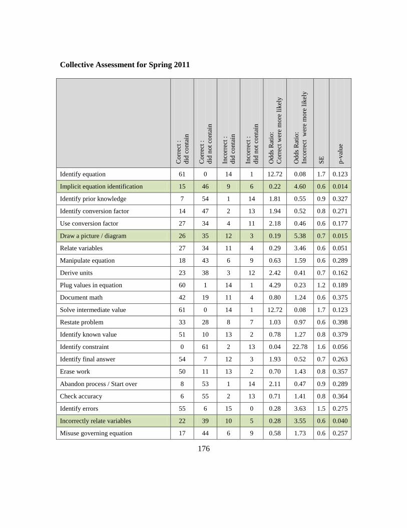
176

Collective Assessment for Spring 2011

Co

rrec

t :

did

co

nta

in

Co

rrec

t :

did

no

t co

nta

in

Inco

rrec

t :

did

co

nta

in

Inco

rrec

t :

did

no

t co

nta

in

Od

ds

Rat

io:

Co

rrec

t w

ere

mo

re l

ikel

y

Od

ds

Rat

io:

Inco

rrec

t w

ere

more

lik

ely

SE

p-v

alu

e

Identify equation 61 0 14 1 12.72 0.08 1.7 0.123

Implicit equation identification 15 46 9 6 0.22 4.60 0.6 0.014

Identify prior knowledge 7 54 1 14 1.81 0.55 0.9 0.327

Identify conversion factor 14 47 2 13 1.94 0.52 0.8 0.271

Use conversion factor 27 34 4 11 2.18 0.46 0.6 0.177

Draw a picture / diagram 26 35 12 3 0.19 5.38 0.7 0.015

Relate variables 27 34 11 4 0.29 3.46 0.6 0.051

Manipulate equation 18 43 6 9 0.63 1.59 0.6 0.289

Derive units 23 38 3 12 2.42 0.41 0.7 0.162

Plug values in equation 60 1 14 1 4.29 0.23 1.2 0.189

Document math 42 19 11 4 0.80 1.24 0.6 0.375

Solve intermediate value 61 0 14 1 12.72 0.08 1.7 0.123

Restate problem 33 28 8 7 1.03 0.97 0.6 0.398

Identify known value 51 10 13 2 0.78 1.27 0.8 0.379

Identify constraint 0 61 2 13 0.04 22.78 1.6 0.056

Identify final answer 54 7 12 3 1.93 0.52 0.7 0.263

Erase work 50 11 13 2 0.70 1.43 0.8 0.357

Abandon process / Start over 8 53 1 14 2.11 0.47 0.9 0.289

Check accuracy 6 55 2 13 0.71 1.41 0.8 0.364

Identify errors 55 6 15 0 0.28 3.63 1.5 0.275

Incorrectly relate variables 22 39 10 5 0.28 3.55 0.6 0.040

Misuse governing equation 17 44 6 9 0.58 1.73 0.6 0.257

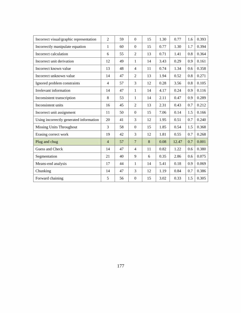
177

Incorrect visual/graphic representation 2 59 0 15 1.30 0.77 1.6 0.393

Incorrectly manipulate equation 1 60 0 15 0.77 1.30 1.7 0.394

Incorrect calculation 6 55 2 13 0.71 1.41 0.8 0.364

Incorrect unit derivation 12 49 1 14 3.43 0.29 0.9 0.161

Incorrect known value 13 48 4 11 0.74 1.34 0.6 0.358

Incorrect unknown value 14 47 2 13 1.94 0.52 0.8 0.271

Ignored problem constraints 4 57 3 12 0.28 3.56 0.8 0.105

Irrelevant information 14 47 1 14 4.17 0.24 0.9 0.116

Inconsistent transcription 8 53 1 14 2.11 0.47 0.9 0.289

Inconsistent units 16 45 2 13 2.31 0.43 0.7 0.212

Incorrect unit assignment 11 50 0 15 7.06 0.14 1.5 0.166

Using incorrectly generated information 20 41 3 12 1.95 0.51 0.7 0.240

Missing Units Throughout 3 58 0 15 1.85 0.54 1.5 0.368

Erasing correct work 19 42 3 12 1.81 0.55 0.7 0.268

Plug and chug 4 57 7 8 0.08 12.47 0.7 0.001

Guess and Check 14 47 4 11 0.82 1.22 0.6 0.380

Segmentation 21 40 9 6 0.35 2.86 0.6 0.075

Means-end analysis 17 44 1 14 5.41 0.18 0.9 0.069

Chunking 14 47 3 12 1.19 0.84 0.7 0.386

Forward chaining 5 56 0 15 3.02 0.33 1.5 0.305

178

Collective Assessment for Fall 2009 and Spring 2011 Combined

Co

rrec

t :

did

co

nta

in

Co

rrec

t :

did

no

t co

nta

in

Inco

rrec

t :

did

co

nta

in

Inco

rrec

t :

did

no

t co

nta

in

Od

ds

Rat

io

Co

rrec

t w

ere

mo

re l

ikel

y

Od

ds

Rat

io

Inco

rrec

t w

ere

more

lik

ely

SE

p-v

alu

e

Identify equation 77 5 54 8 2.28 0.44 0.6 0.143

Implicit equation identification 23 59 40 22 0.21 4.66 0.4 0.000

Identified assumption 1 81 1 61 0.75 1.33 1.2 0.387

Identify prior knowledge 9 73 2 60 3.70 0.27 0.7 0.081

Identify conversion factor 15 67 2 60 6.72 0.15 0.7 0.010

Use conversion factor 37 45 16 46 2.36 0.42 0.4 0.024

Draw a picture / diagram 37 45 27 35 1.07 0.94 0.3 0.392

Make a table 1 81 2 60 0.37 2.70 1.0 0.254

Relate variables 41 41 26 36 1.38 0.72 0.3 0.250

Manipulate equation 18 64 18 44 0.69 1.45 0.4 0.247

Derive units 28 54 10 52 2.70 0.37 0.4 0.021

Plug values in equation 76 6 54 8 1.88 0.53 0.6 0.207

Document math 62 20 40 22 1.71 0.59 0.4 0.138

Solve intermediate value 77 5 56 6 1.65 0.61 0.6 0.283

Identify known value 63 19 38 24 2.09 0.48 0.4 0.052

Identify unknown value 53 29 14 48 6.27 0.16 0.4 0.000

Identify final answer 69 13 43 19 2.35 0.43 0.4 0.043

Labeling / Renaming 43 39 31 31 1.10 0.91 0.3 0.382

Erase work 63 19 42 20 1.58 0.63 0.4 0.189

Abandon process / Start over 8 74 5 57 1.23 0.81 0.6 0.373

Check accuracy 7 75 4 58 1.35 0.74 0.6 0.354

Identify errors 71 11 60 2 0.22 4.65 0.7 0.041

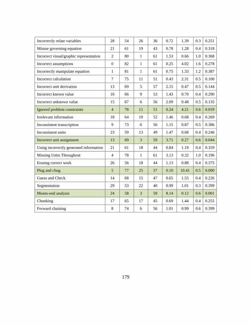
179

Incorrectly relate variables 28 54 26 36 0.72 1.39 0.3 0.251

Misuse governing equation 21 61 19 43 0.78 1.28 0.4 0.318

Incorrect visual/graphic representation 2 80 1 61 1.53 0.66 1.0 0.368

Incorrect assumptions 0 82 1 61 0.25 4.02 1.6 0.278

Incorrectly manipulate equation 1 81 1 61 0.75 1.33 1.2 0.387

Incorrect calculation 7 75 11 51 0.43 2.31 0.5 0.100

Incorrect unit derivation 13 69 5 57 2.15 0.47 0.5 0.144

Incorrect known value 16 66 9 53 1.43 0.70 0.4 0.290

Incorrect unknown value 15 67 6 56 2.09 0.48 0.5 0.135

Ignored problem constraints 4 78 11 51 0.24 4.21 0.6 0.019

Irrelevant information 18 64 10 52 1.46 0.68 0.4 0.269

Inconsistent transcription 9 73 6 56 1.15 0.87 0.5 0.386

Inconsistent units 23 59 13 49 1.47 0.68 0.4 0.246

Incorrect unit assignment 13 69 3 59 3.71 0.27 0.6 0.044

Using incorrectly generated information 21 61 18 44 0.84 1.19 0.4 0.359

Missing Units Throughout 4 78 1 61 3.13 0.32 1.0 0.196

Erasing correct work 26 56 18 44 1.13 0.88 0.4 0.375

Plug and chug 5 77 25 37 0.10 10.41 0.5 0.000

Guess and Check 14 68 15 47 0.65 1.55 0.4 0.226

Segmentation 29 53 22 40 0.99 1.01 0.3 0.399

Means-end analysis 24 58 3 59 8.14 0.12 0.6 0.001

Chunking 17 65 17 45 0.69 1.44 0.4 0.255

Forward chaining 8 74 6 56 1.01 0.99 0.6 0.399

180

Solar Efficiency Problem for Fall 2009 and Spring 2011 Combined

Co

rrec

t :

did

co

nta

in

Co

rrec

t :

did

no

t co

nta

in

Inco

rrec

t :

did

co

nta

in

Inco

rrec

t :

did

no

t co

nta

in

Od

ds

Rat

io

Co

rrec

t w

ere

mo

re l

ikel

y

Od

ds

Rat

io

Inco

rrec

t w

ere

more

lik

ely

SE

p-v

alu

e

Identify equation 29 4 13 4 2.23 0.45 0.7 0.223

Implicit equation identification 6 27 8 9 0.25 4.00 0.6 0.039

Identified assumption 1 32 1 16 0.50 2.00 1.2 0.337

Identify prior knowledge 0 33 0 17 0.52 1.91 2.0 0.379

Identify conversion factor 0 33 0 17 0.52 1.91 2.0 0.379

Use conversion factor 1 32 0 17 1.62 0.62 1.7 0.383

Draw a picture / diagram 13 20 6 11 1.19 0.84 0.6 0.382

Make a table 1 32 2 15 0.23 4.27 1.1 0.161

Relate variables 19 14 7 10 1.94 0.52 0.6 0.213

Manipulate equation 12 21 1 16 9.14 0.11 0.9 0.023

Derive units 0 33 1 16 0.16 6.09 1.7 0.221

Plug values in equation 29 4 14 3 1.55 0.64 0.8 0.340

Document math 20 13 7 10 2.20 0.46 0.6 0.165

Solve intermediate value 31 2 17 0 0.36 2.78 1.6 0.323

Identify known value 28 5 13 4 1.72 0.58 0.7 0.299

Identify unknown value 23 10 5 12 5.52 0.18 0.6 0.010

Identify final answer 32 1 14 3 6.86 0.15 1.0 0.069

Labeling / Renaming 23 10 11 6 1.25 0.80 0.6 0.373

Erase work 29 4 13 4 2.23 0.45 0.7 0.223

Abandon process / Start over 7 26 4 13 0.88 1.14 0.7 0.391

Check accuracy 2 31 0 17 2.78 0.36 1.6 0.323

Identify errors 30 3 16 1 0.63 1.60 1.0 0.359

181

Incorrectly relate variables 22 11 14 3 0.43 2.33 0.7 0.191

Misuse governing equation 16 17 5 12 2.26 0.44 0.6 0.166

Incorrect visual/graphic representation 1 32 0 17 1.62 0.62 1.7 0.383

Incorrect assumptions 0 33 1 16 0.16 6.09 1.7 0.221

Incorrectly manipulate equation 0 33 0 17 0.52 1.91 2.0 0.379

Incorrect calculation 1 32 2 15 0.23 4.27 1.1 0.161

Incorrect unit derivation 0 33 0 17 0.52 1.91 2.0 0.379

Incorrect known value 11 22 5 12 1.20 0.83 0.6 0.382

Incorrect unknown value 12 21 3 14 2.67 0.38 0.7 0.147

Ignored problem constraints 1 32 0 17 1.62 0.62 1.7 0.383

Irrelevant information 16 17 5 12 2.26 0.44 0.6 0.166

Inconsistent transcription 2 31 2 15 0.48 2.07 0.9 0.297

Inconsistent units 0 33 0 17 0.52 1.91 2.0 0.379

Incorrect unit assignment 1 32 0 17 1.62 0.62 1.7 0.383

Using incorrectly generated information 6 27 7 10 0.32 3.15 0.6 0.083

Missing Units Throughout 4 29 0 17 5.34 0.19 1.5 0.218

Erasing correct work 13 20 10 7 0.46 2.20 0.6 0.165

Plug and chug 1 32 2 15 0.23 4.27 1.1 0.161

Guess and Check 2 31 3 14 0.30 3.32 0.9 0.160

Segmentation 27 6 11 6 2.45 0.41 0.7 0.157

Means-end analysis 0 33 0 17 0.52 1.91 2.0 0.379

Chunking 3 30 1 16 1.60 0.63 1.0 0.359

Forward chaining 0 33 0 17 0.52 1.91 2.0 0.379

182

Equivalent Circuit Problem for Fall 2009 and Spring 2011 Combined

Co

rrec

t :

con

tain

ed

Co

rrec

t :

did

no

t co

nta

in

Inco

rrec

t :

con

tain

ed

Inco

rrec

t :

did

no

t co

nta

in

Od

ds

Rat

io

Co

rrec

t w

ere

mo

re l

ikel

y

Od

ds

Rat

io

Inco

rrec

t w

ere

more

lik

ely

SE

p-v

alu

e

Identify equation 15 0 27 3 3.95 0.25 1.5 0.269

Implicit equation identification 15 0 30 0 0.51 1.97 2.0 0.377

Identified assumption 0 15 0 30 1.97 0.51 2.0 0.377

Identify prior knowledge 0 15 0 30 1.97 0.51 2.0 0.377

Identify conversion factor 2 13 1 29 4.46 0.22 1.1 0.154

Use conversion factor 3 12 5 25 1.25 0.80 0.8 0.382

Draw a picture / diagram 10 5 13 17 2.62 0.38 0.6 0.129

Make a table 0 15 0 30 1.97 0.51 2.0 0.377

Relate variables 8 7 12 18 1.71 0.58 0.6 0.274

Manipulate equation 3 12 17 13 0.19 5.23 0.7 0.025

Derive units 0 15 1 29 0.63 1.58 1.7 0.384

Plug values in equation 14 1 26 4 2.15 0.46 1.0 0.297

Document math 13 2 22 8 2.36 0.42 0.8 0.223

Solve intermediate value 15 0 28 2 2.72 0.37 1.6 0.327

Identify known value 7 8 13 17 1.14 0.87 0.6 0.390

Identify unknown value 5 10 5 25 2.50 0.40 0.7 0.172

Identify final answer 12 3 21 9 1.71 0.58 0.7 0.301

Labeling / Renaming 4 11 12 18 0.55 1.83 0.7 0.264

Erase work 12 3 21 9 1.71 0.58 0.7 0.301

Abandon process / Start over 0 15 1 29 0.63 1.58 1.7 0.384

Check accuracy 1 14 3 27 0.64 1.56 1.0 0.364

Identify errors 11 4 30 0 0.04 23.87 1.5 0.047

183

Incorrectly relate variables 3 12 9 21 0.58 1.71 0.7 0.301

Misuse governing equation 3 12 12 18 0.38 2.67 0.7 0.152

Incorrect visual/graphic representation 1 14 1 29 2.07 0.48 1.2 0.332

Incorrect assumptions 0 15 0 30 1.97 0.51 2.0 0.377

Incorrectly manipulate equation 1 14 1 29 2.07 0.48 1.2 0.332

Incorrect calculation 3 12 8 22 0.69 1.45 0.7 0.349

Incorrect unit derivation 0 15 0 30 1.97 0.51 2.0 0.377

Incorrect known value 3 12 3 27 2.25 0.44 0.8 0.247

Incorrect unknown value 2 13 3 27 1.38 0.72 0.9 0.373

Ignored problem constraints 3 12 11 19 0.43 2.32 0.7 0.198

Irrelevant information 0 15 2 28 0.37 2.72 1.6 0.327

Inconsistent transcription 2 13 3 27 1.38 0.72 0.9 0.373

Inconsistent units 1 14 0 30 6.31 0.16 1.7 0.216

Incorrect unit assignment 1 14 0 30 6.31 0.16 1.7 0.216

Using incorrectly generated information 2 13 9 21 0.36 2.79 0.8 0.172

Missing Units Throughout 0 15 1 29 0.63 1.58 1.7 0.384

Erasing correct work 4 11 6 24 1.45 0.69 0.7 0.347

Plug and chug 3 12 15 15 0.25 4.00 0.7 0.057

Guess and Check 11 4 10 20 5.50 0.18 0.7 0.016

Segmentation 2 13 11 19 0.27 3.76 0.8 0.095

Means-end analysis 0 15 0 30 1.97 0.51 2.0 0.377

Chunking 13 2 16 14 5.69 0.18 0.8 0.033

Forward chaining 1 14 5 25 0.36 2.80 1.0 0.229

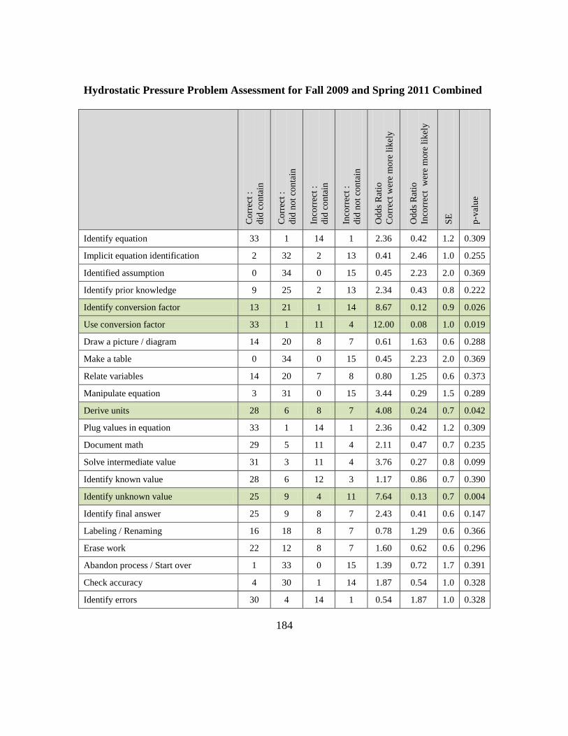
184

Hydrostatic Pressure Problem Assessment for Fall 2009 and Spring 2011 Combined

Co

rrec

t :

did

co

nta

in

Co

rrec

t :

did

no

t co

nta

in

Inco

rrec

t :

did

co

nta

in

Inco

rrec

t :

did

no

t co

nta

in

Od

ds

Rat

io

Co

rrec

t w

ere

mo

re l

ikel

y

Od

ds

Rat

io

Inco

rrec

t w

ere

more

lik

ely

SE

p-v

alu

e

Identify equation 33 1 14 1 2.36 0.42 1.2 0.309

Implicit equation identification 2 32 2 13 0.41 2.46 1.0 0.255

Identified assumption 0 34 0 15 0.45 2.23 2.0 0.369

Identify prior knowledge 9 25 2 13 2.34 0.43 0.8 0.222

Identify conversion factor 13 21 1 14 8.67 0.12 0.9 0.026

Use conversion factor 33 1 11 4 12.00 0.08 1.0 0.019

Draw a picture / diagram 14 20 8 7 0.61 1.63 0.6 0.288

Make a table 0 34 0 15 0.45 2.23 2.0 0.369

Relate variables 14 20 7 8 0.80 1.25 0.6 0.373

Manipulate equation 3 31 0 15 3.44 0.29 1.5 0.289

Derive units 28 6 8 7 4.08 0.24 0.7 0.042

Plug values in equation 33 1 14 1 2.36 0.42 1.2 0.309

Document math 29 5 11 4 2.11 0.47 0.7 0.235

Solve intermediate value 31 3 11 4 3.76 0.27 0.8 0.099

Identify known value 28 6 12 3 1.17 0.86 0.7 0.390

Identify unknown value 25 9 4 11 7.64 0.13 0.7 0.004

Identify final answer 25 9 8 7 2.43 0.41 0.6 0.147

Labeling / Renaming 16 18 8 7 0.78 1.29 0.6 0.366

Erase work 22 12 8 7 1.60 0.62 0.6 0.296

Abandon process / Start over 1 33 0 15 1.39 0.72 1.7 0.391

Check accuracy 4 30 1 14 1.87 0.54 1.0 0.328

Identify errors 30 4 14 1 0.54 1.87 1.0 0.328

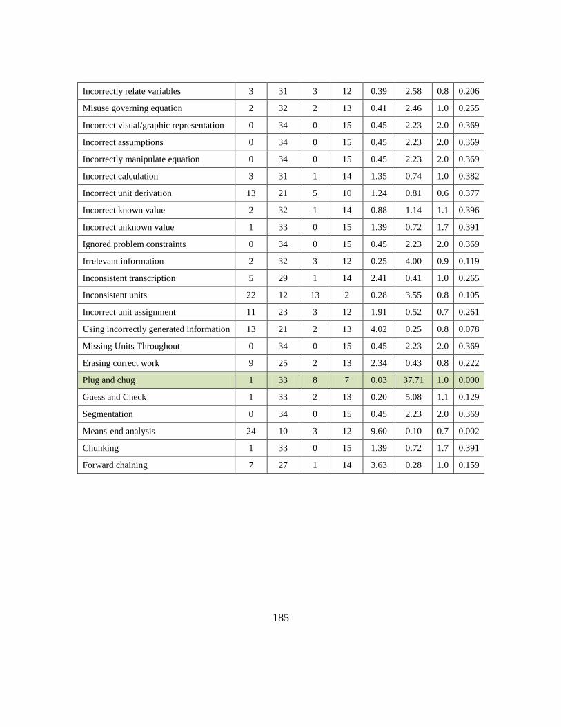
185

Incorrectly relate variables 3 31 3 12 0.39 2.58 0.8 0.206

Misuse governing equation 2 32 2 13 0.41 2.46 1.0 0.255

Incorrect visual/graphic representation 0 34 0 15 0.45 2.23 2.0 0.369

Incorrect assumptions 0 34 0 15 0.45 2.23 2.0 0.369

Incorrectly manipulate equation 0 34 0 15 0.45 2.23 2.0 0.369

Incorrect calculation 3 31 1 14 1.35 0.74 1.0 0.382

Incorrect unit derivation 13 21 5 10 1.24 0.81 0.6 0.377

Incorrect known value 2 32 1 14 0.88 1.14 1.1 0.396

Incorrect unknown value 1 33 0 15 1.39 0.72 1.7 0.391

Ignored problem constraints 0 34 0 15 0.45 2.23 2.0 0.369

Irrelevant information 2 32 3 12 0.25 4.00 0.9 0.119

Inconsistent transcription 5 29 1 14 2.41 0.41 1.0 0.265

Inconsistent units 22 12 13 2 0.28 3.55 0.8 0.105

Incorrect unit assignment 11 23 3 12 1.91 0.52 0.7 0.261

Using incorrectly generated information 13 21 2 13 4.02 0.25 0.8 0.078

Missing Units Throughout 0 34 0 15 0.45 2.23 2.0 0.369

Erasing correct work 9 25 2 13 2.34 0.43 0.8 0.222

Plug and chug 1 33 8 7 0.03 37.71 1.0 0.000

Guess and Check 1 33 2 13 0.20 5.08 1.1 0.129

Segmentation 0 34 0 15 0.45 2.23 2.0 0.369

Means-end analysis 24 10 3 12 9.60 0.10 0.7 0.002

Chunking 1 33 0 15 1.39 0.72 1.7 0.391

Forward chaining 7 27 1 14 3.63 0.28 1.0 0.159

186

APPENDIX H

SIGNIFICANT EFFECTS OF PRESENCE OF PROBLEM SOLVING FEATURES

ON PROBLEM SOLVING SUCCESS FROM THE LINEAR MIXED EFFECTS MODELS

Each table represents a separate regression model.

The intercept is representative of the neutral condition where the solution was completed

for problem 1 in the first semester and did not utilize the problem feature. Each line of

the table represents the impact of a change to that neutral condition. The value should

only be interpreted in terms of the magnitude (large or small) and direction (positive of

negative). The actual numeric value cannot be directly interpreted. Positive values are

associated with correct solutions and large magnitudes indicate a stronger effect.

Problem 2-1 represents the effect attributed to problem 2 (over problem 1)

Problem 3-2 represents the effect attributed to problem 2 (over problem 2)

The effect from problem 3 over problem 1 is redundant and can be inferred from

summing the effects of Problem 2-1 and Problem 3-2.

Semester Intervention-None indicated the effect attributed to the intervention

The remaining effect is the effect attributed to the problem feature where 1-0 indicates

that the effect is due to the presence of the feature compared to not using the feature.

187

Features attributed to successful solutions

Value Std.Error DF t-value p-value

Intercept -0.614 0.651 78 -0.943 0.349

Problem 2-1 -4.413 0.656 78 -6.731 0.000

Problem 3-2 -2.057 0.845 78 -2.434 0.017

Semester Intervention-None 4.379 0.888 61 4.932 0.000

Use conversion factor 1-0 2.624 0.811 78 3.236 0.002

Value Std.Error DF t-value p-value

Intercept -1.339 0.627 78 -2.136 0.036

Problem 2-1 -2.504 0.738 78 -3.393 0.001

Problem 3-2 -0.231 0.603 78 -0.383 0.703

Semester Intervention-None 2.886 0.596 61 4.840 0.000

Document math 1-0 1.461 0.650 78 2.249 0.027

Value Std.Error DF t-value p-value

Intercept -0.400 0.397 78 -1.006 0.317

Problem 2-1 -1.916 0.584 78 -3.283 0.002

Problem 3-2 -0.855 0.660 78 -1.295 0.199

Semester Intervention-None 2.583 0.506 61 5.104 0.000

Means ends analysis 1-0 2.214 0.887 78 2.494 0.015

Value Std.Error DF t-value p-value

Intercept -0.659 0.447 78 -1.476 0.144

Problem 2-1 -3.092 0.858 78 -3.603 0.001

Problem 3-2 0.325 0.577 78 0.562 0.576

Semester Intervention-None 2.734 0.534 61 5.120 0.000

Chunking 1-0 1.868 0.828 78 2.257 0.027

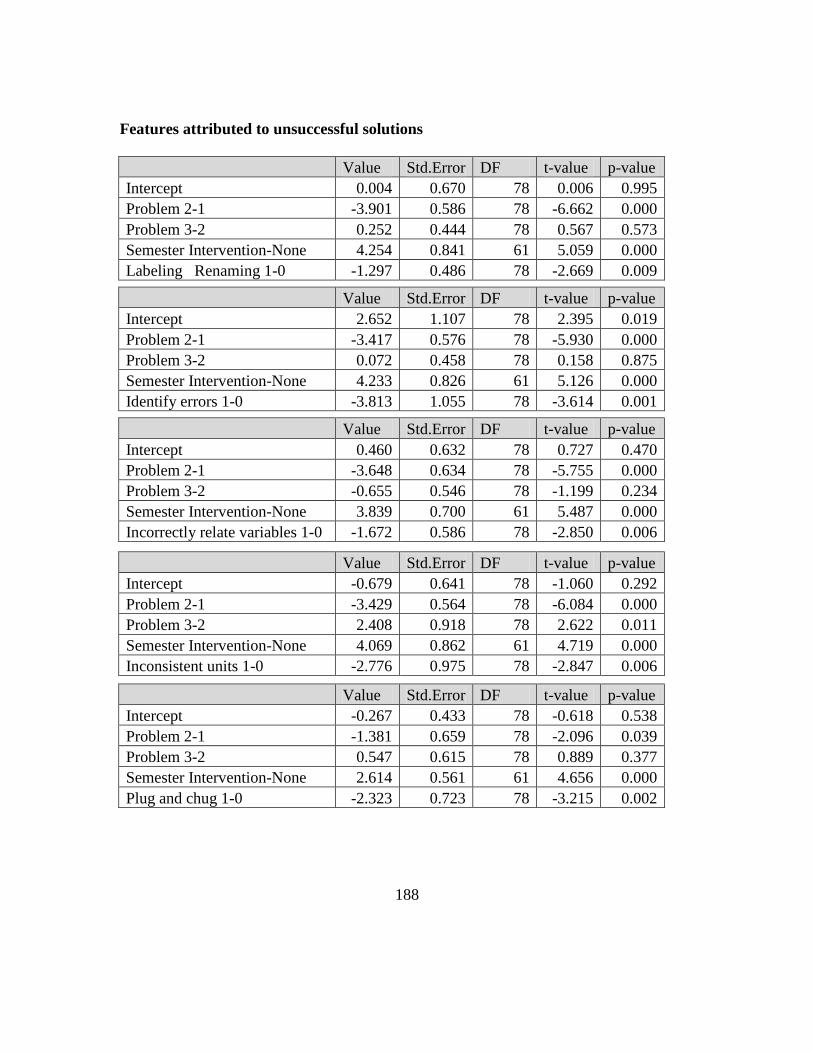
188

Features attributed to unsuccessful solutions

Value Std.Error DF t-value p-value

Intercept 0.004 0.670 78 0.006 0.995

Problem 2-1 -3.901 0.586 78 -6.662 0.000

Problem 3-2 0.252 0.444 78 0.567 0.573

Semester Intervention-None 4.254 0.841 61 5.059 0.000

Labeling Renaming 1-0 -1.297 0.486 78 -2.669 0.009

Value Std.Error DF t-value p-value

Intercept 2.652 1.107 78 2.395 0.019

Problem 2-1 -3.417 0.576 78 -5.930 0.000

Problem 3-2 0.072 0.458 78 0.158 0.875

Semester Intervention-None 4.233 0.826 61 5.126 0.000

Identify errors 1-0 -3.813 1.055 78 -3.614 0.001

Value Std.Error DF t-value p-value

Intercept 0.460 0.632 78 0.727 0.470

Problem 2-1 -3.648 0.634 78 -5.755 0.000

Problem 3-2 -0.655 0.546 78 -1.199 0.234

Semester Intervention-None 3.839 0.700 61 5.487 0.000

Incorrectly relate variables 1-0 -1.672 0.586 78 -2.850 0.006

Value Std.Error DF t-value p-value

Intercept -0.679 0.641 78 -1.060 0.292

Problem 2-1 -3.429 0.564 78 -6.084 0.000

Problem 3-2 2.408 0.918 78 2.622 0.011

Semester Intervention-None 4.069 0.862 61 4.719 0.000

Inconsistent units 1-0 -2.776 0.975 78 -2.847 0.006

Value Std.Error DF t-value p-value

Intercept -0.267 0.433 78 -0.618 0.538

Problem 2-1 -1.381 0.659 78 -2.096 0.039

Problem 3-2 0.547 0.615 78 0.889 0.377

Semester Intervention-None 2.614 0.561 61 4.656 0.000

Plug and chug 1-0 -2.323 0.723 78 -3.215 0.002

189

APPENDIX I

SIGNIFICANT EFFECTS OF PROCESS MEASURES

ON PROBLEM SOLVING SUCCESS FROM THE LINEAR MIXED EFFECTS MODELS

Value Std.Error DF t-value p-value

Intercept -0.978 0.565 78 -1.732 0.087

Problem 2-1 -3.336 0.584 78 -5.708 0.000

Problem 3-2 0.059 0.459 78 0.129 0.898

Semester 3.486 0.719 61 4.850 0.000

Correct representation 1-0 1.417 0.501 78 2.829 0.006

Value Std.Error DF t-value p-value

Intercept -2.646 0.899 77 -2.943 0.004

Problem 2-1 -1.857 0.751 77 -2.472 0.016

Problem 3-2 0.479 0.744 77 0.644 0.522

Semester 2.948 0.695 61 4.243 0.000

Strategy Intermediate - Basic 2.444 0.793 77 3.081 0.003

Strategy Advanced- Intermediate 3.250 1.133 77 2.870 0.005

Value Std.Error DF t-value p-value

Intercept -6.995 1.378 78 -5.076 0.000

Problem 2-1 -5.247 0.700 78 -7.497 0.000

Problem 3-2 0.319 0.415 78 0.768 0.445

Semester 6.691 1.218 61 5.494 0.000

Correct known values 1-0 6.414 1.169 78 5.488 0.000

Value Std.Error DF t-value p-value

Intercept -1.596 0.709 78 -2.251 0.027

Problem 2-1 -3.328 0.568 78 -5.862 0.000

Problem 3-2 1.064 0.486 78 2.192 0.031

Semester 4.568 0.911 61 5.013 0.000

Number of tries to achieve correct

known values 3.875 0.934 78 4.149 0.000

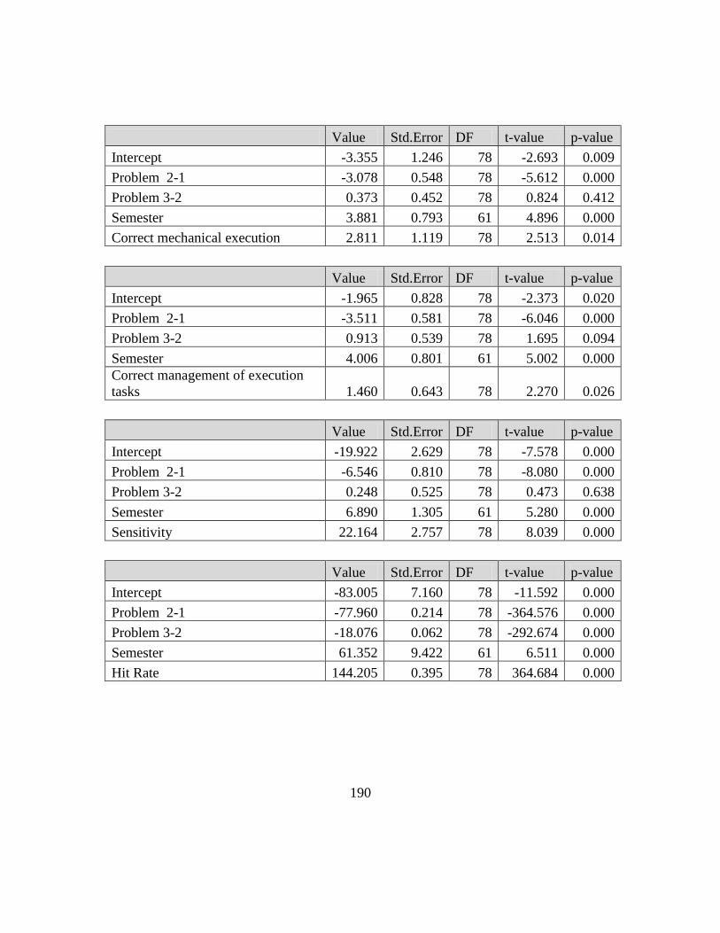
190

Value Std.Error DF t-value p-value

Intercept -3.355 1.246 78 -2.693 0.009

Problem 2-1 -3.078 0.548 78 -5.612 0.000

Problem 3-2 0.373 0.452 78 0.824 0.412

Semester 3.881 0.793 61 4.896 0.000

Correct mechanical execution 2.811 1.119 78 2.513 0.014

Value Std.Error DF t-value p-value

Intercept -1.965 0.828 78 -2.373 0.020

Problem 2-1 -3.511 0.581 78 -6.046 0.000

Problem 3-2 0.913 0.539 78 1.695 0.094

Semester 4.006 0.801 61 5.002 0.000

Correct management of execution

tasks 1.460 0.643 78 2.270 0.026

Value Std.Error DF t-value p-value

Intercept -19.922 2.629 78 -7.578 0.000

Problem 2-1 -6.546 0.810 78 -8.080 0.000

Problem 3-2 0.248 0.525 78 0.473 0.638

Semester 6.890 1.305 61 5.280 0.000

Sensitivity 22.164 2.757 78 8.039 0.000

Value Std.Error DF t-value p-value

Intercept -83.005 7.160 78 -11.592 0.000

Problem 2-1 -77.960 0.214 78 -364.576 0.000

Problem 3-2 -18.076 0.062 78 -292.674 0.000

Semester 61.352 9.422 61 6.511 0.000

Hit Rate 144.205 0.395 78 364.684 0.000

191

APPENDIX J

SIGNIFICANT EFFECTS OF OUTCOME MEASURES

ON PROBLEM SOLVING SUCCESS FROM THE LINEAR MIXED EFFECTS MODEL

Value Std.Error DF t-value p-value

Intercept 0.991 0.647 78 1.532 0.130

Problem 2-1 -4.386 0.702 78 -6.251 0.000

Problem 3-2 -1.129 0.587 78 -1.924 0.058

Semester 3.967 0.730 61 5.433 0.000

Conceptual Errors -2.502 0.525 78 -4.767 0.000

Value Std.Error DF t-value p-value

Intercept -0.583 0.583 78 -1.000 0.320

Problem 2-1 -3.078 0.548 78 -5.622 0.000

Problem 3-2 0.454 0.455 78 0.996 0.323

Semester 3.936 0.793 61 4.965 0.000

Mechanical Errors -2.551 0.931 78 -2.741 0.008

Value Std.Error DF t-value p-value

Intercept 0.947 0.866 78 1.092 0.278

Problem 2-1 -6.021 0.783 78 -7.692 0.000

Problem 3-2 0.097 0.456 78 0.212 0.833

Semester 6.104 1.177 61 5.187 0.000

Management Errors -1.397 0.246 78 -5.671 0.000

Value Std.Error DF t-value p-value

Intercept 6.836 1.532 78 4.462 0.000

Problem 2-1 -9.887 1.056 78 -9.367 0.000

Problem 3-2 -0.260 0.470 78 -0.554 0.581

Semester 6.499 1.716 61 3.788 0.000

Error Rate -34.579 4.106 78 -8.421 0.000

192

APPENDIX K

SIGNIFICANT EFFECTS OF PROBLEM SOLVING FEATURES ON MENTAL WORKLOAD

MEASURES FROM LINEAR MIXED EFFECTS MODELS

NOTES ON INTERPRETING RESULTS:

Each table represents a separate regression model.

The intercept is representative of the neutral condition where the solution was completed

for problem 1 and did not utilize the problem feature. Each line of the table represents

the impact of a change to that neutral condition. The value should only be interpreted in

terms of the magnitude (large or small) and direction (positive of negative). The actual

numeric value cannot be directly interpreted. Positive values are associated with correct

solutions and large magnitudes indicate a stronger effect.

Problem 2-1 represents the effect attributed to problem 2 (over problem 1)

Problem 3-2 represents the effect attributed to problem 2 (over problem 2)

The effect from problem 3 over problem 1 is redundant and can be inferred from

summing the effects of Problem 2-1 and Problem 3-2.

The remaining effect is the effect attributed to the problem feature where 1-0 indicates

that the effect is due to the presence of the feature compared to not using the feature.

193

Significant Effects of Problem Solving Features on Overall Mental Workload

Value Std.Error DF t-value p-value

Intercept 76.966 14.528 34 5.298 0.000

Problem 2-1 -5.248 3.599 34 -1.458 0.154

Problem 3-2 -3.521 3.390 34 -1.039 0.306

Identify equation 1-0 -30.281 14.158 34 -2.139 0.040

Value Std.Error DF t-value p-value

Intercept 69.051 11.186 34 6.173 0.000

Problem 2-1 -5.502 3.626 34 -1.518 0.138

Problem 3-2 -3.386 3.383 34 -1.001 0.324

Plug values in equation 1-0 -22.734 10.889 34 -2.088 0.044

Value Std.Error DF t-value p-value

Intercept 36.022 5.922 34 6.082 0.000

Problem 2-1 0.728 4.178 34 0.174 0.863

Problem 3-2 -3.279 3.440 34 -0.953 0.347

Identify known value 1-0 10.859 5.247 34 2.069 0.046

Value Std.Error DF t-value p-value

Intercept 41.747 3.786 34 11.027 0.000

Problem 2-1 -1.662 3.606 34 -0.461 0.648

Problem 3-2 1.455 3.948 34 0.369 0.715

Misuse governing equation 1-0 8.677 4.116 34 2.108 0.043

Value Std.Error DF t-value p-value

Intercept 46.786 3.019 34 15.495 0.000

Problem 2-1 -3.605 3.500 34 -1.030 0.310

Problem 3-2 -8.792 4.305 34 -2.042 0.049

Incorrect unit derivation 1-0 11.804 5.557 34 2.124 0.041

Value Std.Error DF t-value p-value

Intercept 43.163 2.999 34 14.393 0.000

Problem 2-1 -2.148 3.143 34 -0.683 0.499

Problem 3-2 -7.016 3.179 34 -2.207 0.034

Using incorrectly generated information 1-0 15.246 3.831 34 3.980 0.000

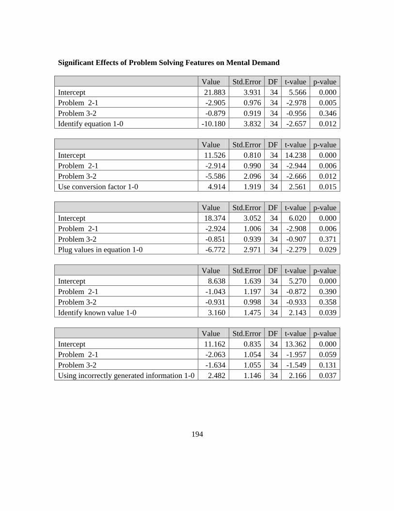
194

Significant Effects of Problem Solving Features on Mental Demand

Value Std.Error DF t-value p-value

Intercept 21.883 3.931 34 5.566 0.000

Problem 2-1 -2.905 0.976 34 -2.978 0.005

Problem 3-2 -0.879 0.919 34 -0.956 0.346

Identify equation 1-0 -10.180 3.832 34 -2.657 0.012

Value Std.Error DF t-value p-value

Intercept 11.526 0.810 34 14.238 0.000

Problem 2-1 -2.914 0.990 34 -2.944 0.006

Problem 3-2 -5.586 2.096 34 -2.666 0.012

Use conversion factor 1-0 4.914 1.919 34 2.561 0.015

Value Std.Error DF t-value p-value

Intercept 18.374 3.052 34 6.020 0.000

Problem 2-1 -2.924 1.006 34 -2.908 0.006

Problem 3-2 -0.851 0.939 34 -0.907 0.371

Plug values in equation 1-0 -6.772 2.971 34 -2.279 0.029

Value Std.Error DF t-value p-value

Intercept 8.638 1.639 34 5.270 0.000

Problem 2-1 -1.043 1.197 34 -0.872 0.390

Problem 3-2 -0.931 0.998 34 -0.933 0.358

Identify known value 1-0 3.160 1.475 34 2.143 0.039

Value Std.Error DF t-value p-value

Intercept 11.162 0.835 34 13.362 0.000

Problem 2-1 -2.063 1.054 34 -1.957 0.059

Problem 3-2 -1.634 1.055 34 -1.549 0.131

Using incorrectly generated information 1-0 2.482 1.146 34 2.166 0.037

195

Significant Effects of Problem Solving Features on Temporal Demand

Value Std.Error DF t-value p-value

Intercept 5.964 1.875 34 3.181 0.003

Problem 2-1 2.112 1.476 34 1.431 0.162

Problem 3-2 -1.938 1.268 34 -1.528 0.136

Identify known value 1-0 3.568 1.713 34 2.083 0.045

Value Std.Error DF t-value p-value

Intercept 9.325 0.893 34 10.438 0.000

Problem 2-1 0.922 1.243 34 0.742 0.463

Problem 3-2 1.030 1.791 34 0.575 0.569

Inconsistent units 1-0 -3.927 1.846 34 -2.128 0.041

Value Std.Error DF t-value p-value

Intercept 8.678 0.936 34 9.274 0.000

Problem 2-1 0.949 1.212 34 0.783 0.439

Problem 3-2 -2.618 1.211 34 -2.162 0.038

Using incorrectly generated information 1-0 3.078 1.286 34 2.395 0.022

Value Std.Error DF t-value p-value

Intercept 9.390 0.892 34 10.527 0.000

Problem 2-1 0.680 1.230 34 0.553 0.584

Problem 3-2 1.283 1.837 34 0.698 0.490

Means ends analysis 1-0 -4.397 1.998 34 -2.201 0.035

196

Significant Effects of Problem Solving Features on Performance

Value Std.Error DF t-value p-value

Intercept 2.956 0.878 34 3.367 0.002

Problem 2-1 0.658 0.986 34 0.668 0.509

Problem 3-2 1.561 0.998 34 1.564 0.127

Incorrectly relate variables 1-0 2.560 0.852 34 3.006 0.005

Value Std.Error DF t-value p-value

Intercept 3.547 0.794 34 4.465 0.000

Problem 2-1 0.656 1.016 34 0.645 0.523

Problem 3-2 1.387 1.009 34 1.375 0.178

Incorrect unknown value 1-0 2.773 1.054 34 2.631 0.013

Value Std.Error DF t-value p-value

Intercept 3.884 0.619 34 6.277 0.000

Problem 2-1 0.450 0.749 34 0.601 0.552

Problem 3-2 -0.866 0.752 34 -1.152 0.257

Using incorrectly generated information 1-0 4.423 0.842 34 5.256 0.000

197

Significant Effects of Problem Solving Features on Effort

Value Std.Error DF t-value p-value

Intercept 21.002 3.457 34 6.076 0.000

Problem 2-1 -1.823 0.843 34 -2.162 0.038

Problem 3-2 -0.780 0.793 34 -0.984 0.332

Identify equation 1-0 -8.262 3.361 34 -2.458 0.019

Value Std.Error DF t-value p-value

Intercept 12.561 0.738 34 17.022 0.000

Problem 2-1 -1.942 0.809 34 -2.401 0.022

Problem 3-2 -5.371 1.735 34 -3.095 0.004

Use conversion factor 1-0 4.827 1.589 34 3.038 0.005

Value Std.Error DF t-value p-value

Intercept 18.441 2.723 34 6.773 0.000

Problem 2-1 -1.844 0.857 34 -2.151 0.039

Problem 3-2 -0.742 0.800 34 -0.927 0.360

Plug values in equation 1-0 -5.806 2.650 34 -2.191 0.035

Value Std.Error DF t-value p-value

Intercept 10.063 1.430 34 7.039 0.000

Problem 2-1 -0.276 0.991 34 -0.279 0.782

Problem 3-2 -0.698 0.811 34 -0.860 0.396

Identify known value 1-0 2.716 1.254 34 2.166 0.038

Value Std.Error DF t-value p-value

Intercept 12.679 0.736 34 17.228 0.000

Problem 2-1 0.854 1.372 34 0.622 0.538

Problem 3-2 -0.580 0.828 34 -0.700 0.489

Chunking 1-0 -3.091 1.474 34 -2.097 0.044

198

Significant Effects of Problem Solving Features on Frustration

Value Std.Error DF t-value p-value

Intercept 6.404 1.055 34 6.073 0.000

Problem 2-1 0.005 0.934 34 0.005 0.996

Problem 3-2 1.116 1.030 34 1.083 0.286

Misuse governing equation 1-0 2.870 1.096 34 2.619 0.013

Value Std.Error DF t-value p-value

Intercept 7.940 0.912 34 8.704 0.000

Problem 2-1 -1.526 0.895 34 -1.705 0.097

Problem 3-2 -0.554 0.812 34 -0.683 0.499

Incorrect calculation 1-0 4.274 1.477 34 2.894 0.007

Value Std.Error DF t-value p-value

Intercept 8.070 0.862 34 9.361 0.000

Problem 2-1 -0.600 0.907 34 -0.661 0.513

Problem 3-2 -2.304 1.131 34 -2.038 0.049

Incorrect unit derivation 1-0 3.954 1.472 34 2.686 0.011

Value Std.Error DF t-value p-value

Intercept 7.326 0.898 34 8.158 0.000

Problem 2-1 -0.336 0.909 34 -0.370 0.714

Problem 3-2 -1.202 0.921 34 -1.305 0.201

Using incorrectly generated information 1-0 3.011 1.124 34 2.679 0.011

Value Std.Error DF t-value p-value

Intercept 7.958 0.870 34 9.150 0.000

Problem 2-1 -1.536 1.016 34 -1.513 0.140

Problem 3-2 -0.597 0.899 34 -0.664 0.511

Plug and chug 1-0 3.202 1.453 34 2.204 0.034

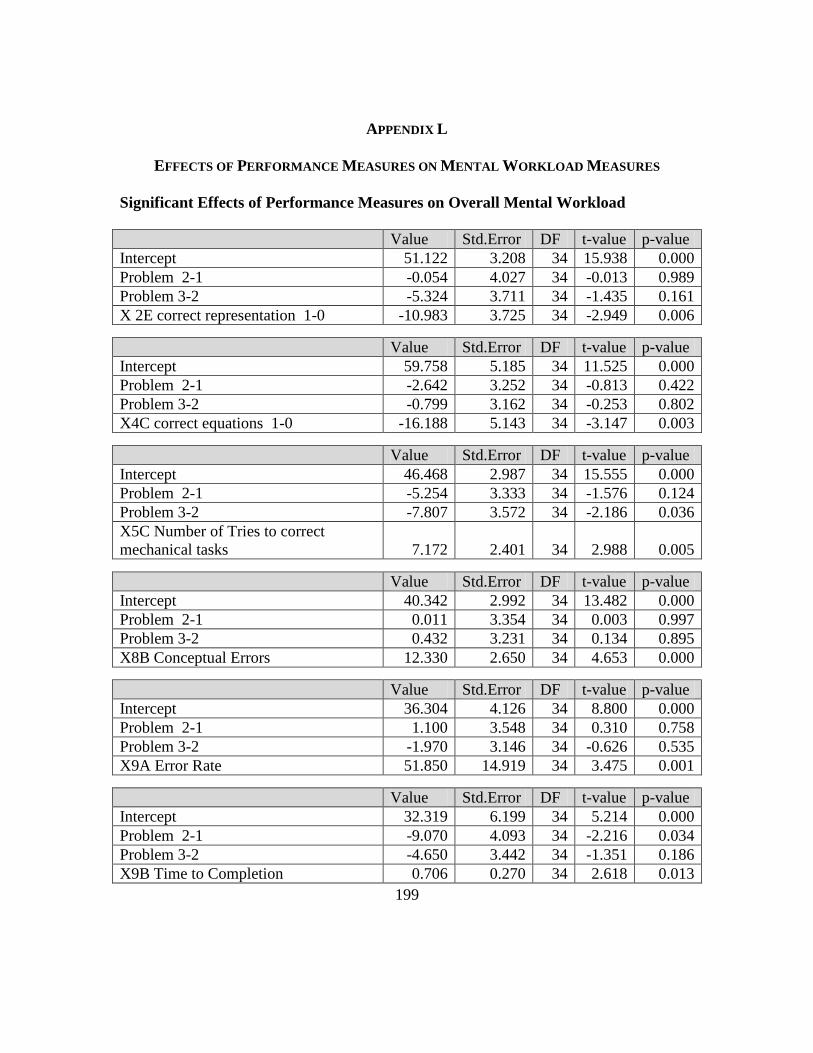
199

APPENDIX L

EFFECTS OF PERFORMANCE MEASURES ON MENTAL WORKLOAD MEASURES

Significant Effects of Performance Measures on Overall Mental Workload

Value Std.Error DF t-value p-value

Intercept 51.122 3.208 34 15.938 0.000

Problem 2-1 -0.054 4.027 34 -0.013 0.989

Problem 3-2 -5.324 3.711 34 -1.435 0.161

X 2E correct representation 1-0 -10.983 3.725 34 -2.949 0.006

Value Std.Error DF t-value p-value

Intercept 59.758 5.185 34 11.525 0.000

Problem 2-1 -2.642 3.252 34 -0.813 0.422

Problem 3-2 -0.799 3.162 34 -0.253 0.802

X4C correct equations 1-0 -16.188 5.143 34 -3.147 0.003

Value Std.Error DF t-value p-value

Intercept 46.468 2.987 34 15.555 0.000

Problem 2-1 -5.254 3.333 34 -1.576 0.124

Problem 3-2 -7.807 3.572 34 -2.186 0.036

X5C Number of Tries to correct

mechanical tasks 7.172 2.401 34 2.988 0.005

Value Std.Error DF t-value p-value

Intercept 40.342 2.992 34 13.482 0.000

Problem 2-1 0.011 3.354 34 0.003 0.997

Problem 3-2 0.432 3.231 34 0.134 0.895

X8B Conceptual Errors 12.330 2.650 34 4.653 0.000

Value Std.Error DF t-value p-value

Intercept 36.304 4.126 34 8.800 0.000

Problem 2-1 1.100 3.548 34 0.310 0.758

Problem 3-2 -1.970 3.146 34 -0.626 0.535

X9A Error Rate 51.850 14.919 34 3.475 0.001

Value Std.Error DF t-value p-value

Intercept 32.319 6.199 34 5.214 0.000

Problem 2-1 -9.070 4.093 34 -2.216 0.034

Problem 3-2 -4.650 3.442 34 -1.351 0.186

X9B Time to Completion 0.706 0.270 34 2.618 0.013

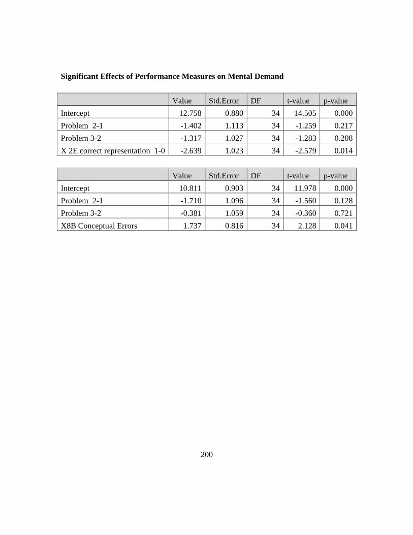
200

Significant Effects of Performance Measures on Mental Demand

Value Std.Error DF t-value p-value

Intercept 12.758 0.880 34 14.505 0.000

Problem 2-1 -1.402 1.113 34 -1.259 0.217

Problem 3-2 -1.317 1.027 34 -1.283 0.208

X 2E correct representation 1-0 -2.639 1.023 34 -2.579 0.014

Value Std.Error DF t-value p-value

Intercept 10.811 0.903 34 11.978 0.000

Problem 2-1 -1.710 1.096 34 -1.560 0.128

Problem 3-2 -0.381 1.059 34 -0.360 0.721

X8B Conceptual Errors 1.737 0.816 34 2.128 0.041

201

Significant Effects of Performance Measures on Temporal Demand

Value Std.Error DF t-value p-value

Intercept 10.428 0.992 34 10.510 0.000

Problem 2-1 1.608 1.381 34 1.164 0.253

Problem 3-2 -2.226 1.286 34 -1.732 0.092

X 2E correct representation 1-0 -2.664 1.153 34 -2.310 0.027

Value Std.Error DF t-value p-value

Intercept 7.655 0.956 34 8.006 0.000

Problem 2-1 1.828 1.210 34 1.511 0.140

Problem 3-2 -0.631 1.170 34 -0.539 0.593

X8B Conceptual Errors 3.256 0.870 34 3.742 0.001

Value Std.Error DF t-value p-value

Intercept 8.070 1.020 34 7.915 0.000

Problem 2-1 1.384 1.303 34 1.062 0.296

Problem 3-2 -2.341 1.240 34 -1.889 0.068

X8D Management Errors 0.889 0.349 34 2.547 0.016

Value Std.Error DF t-value p-value

Intercept 6.939 1.318 34 5.263 0.000

Problem 2-1 1.923 1.304 34 1.474 0.150

Problem 3-2 -1.447 1.160 34 -1.247 0.221

X9A Error Rate 11.983 4.816 34 2.488 0.018

Value Std.Error DF t-value p-value

Intercept 5.349 1.878 34 2.848 0.007

Problem 2-1 -0.812 1.422 34 -0.571 0.572

Problem 3-2 -2.256 1.242 34 -1.817 0.078

X9B Time to Completion 0.200 0.082 34 2.439 0.020

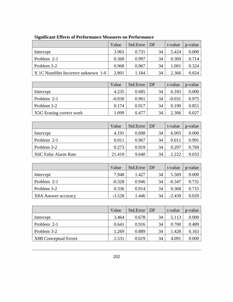
202

Significant Effects of Performance Measures on Performance

Value Std.Error DF t-value p-value

Intercept 3.965 0.731 34 5.424 0.000

Problem 2-1 0.368 0.997 34 0.369 0.714

Problem 3-2 0.968 0.967 34 1.001 0.324

X 1C NumHits Incorrect unknown 1-0 2.801 1.184 34 2.366 0.024

Value Std.Error DF t-value p-value

Intercept 4.235 0.685 34 6.183 0.000

Problem 2-1 -0.030 0.961 34 -0.031 0.975

Problem 3-2 0.174 0.917 34 0.190 0.851

X5G Erasing correct work 1.099 0.477 34 2.306 0.027

Value Std.Error DF t-value p-value

Intercept 4.191 0.698 34 6.005 0.000

Problem 2-1 0.011 0.967 34 0.011 0.991

Problem 3-2 0.273 0.919 34 0.297 0.769

X6C False Alarm Rate 21.419 9.640 34 2.222 0.033

Value Std.Error DF t-value p-value

Intercept 7.948 1.427 34 5.569 0.000

Problem 2-1 -0.328 0.946 34 -0.347 0.731

Problem 3-2 0.336 0.914 34 0.368 0.715

X8A Answer accuracy -3.528 1.446 34 -2.439 0.020

Value Std.Error DF t-value p-value

Intercept 3.464 0.678 34 5.113 0.000

Problem 2-1 0.641 0.916 34 0.700 0.489

Problem 3-2 1.269 0.889 34 1.428 0.163

X8B Conceptual Errors 2.531 0.619 34 4.091 0.000

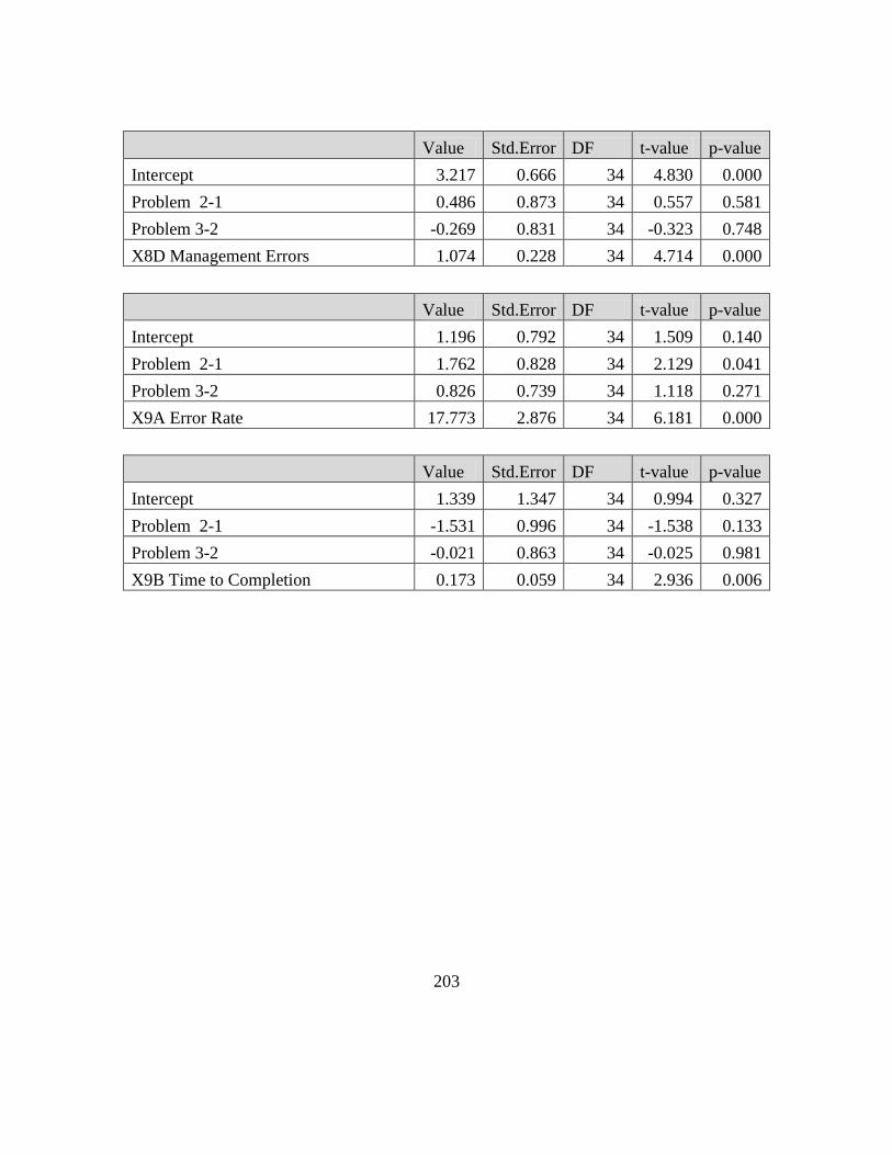
203

Value Std.Error DF t-value p-value

Intercept 3.217 0.666 34 4.830 0.000

Problem 2-1 0.486 0.873 34 0.557 0.581

Problem 3-2 -0.269 0.831 34 -0.323 0.748

X8D Management Errors 1.074 0.228 34 4.714 0.000

Value Std.Error DF t-value p-value

Intercept 1.196 0.792 34 1.509 0.140

Problem 2-1 1.762 0.828 34 2.129 0.041

Problem 3-2 0.826 0.739 34 1.118 0.271

X9A Error Rate 17.773 2.876 34 6.181 0.000

Value Std.Error DF t-value p-value

Intercept 1.339 1.347 34 0.994 0.327

Problem 2-1 -1.531 0.996 34 -1.538 0.133

Problem 3-2 -0.021 0.863 34 -0.025 0.981

X9B Time to Completion 0.173 0.059 34 2.936 0.006

204

Significant Effects of Performance Measures on Effort

Value Std.Error DF t-value p-value

Intercept 13.273 0.827 33 16.057 0.000

Problem 2-1 -0.607 0.918 33 -0.661 0.513

Problem 3-2 -0.743 0.855 33 -0.870 0.391

X 2D Explicit visual 0 5 -5.958 2.122 33 -2.807 0.008

X 2D Explicit visual 1-0 -1.054 0.896 33 -1.176 0.248

Value Std.Error DF t-value p-value

Intercept 13.714 0.796 34 17.228 0.000

Problem 2-1 -0.558 0.917 34 -0.608 0.547

Problem 3-2 -1.080 0.841 34 -1.285 0.208

X 2E correct representation 1-0 -2.447 0.895 34 -2.736 0.010

Value Std.Error DF t-value p-value

Intercept 15.428 1.295 34 11.910 0.000

Problem 2-1 -1.172 0.836 34 -1.402 0.170

Problem 3-2 -0.278 0.814 34 -0.342 0.735

X4C correct equations 1-0 -3.310 1.301 34 -2.544 0.016

Value Std.Error DF t-value p-value

Intercept 11.747 0.802 34 14.646 0.000

Problem 2-1 -0.829 0.865 34 -0.959 0.345

Problem 3-2 -0.147 0.833 34 -0.176 0.861

X8B Conceptual Errors 1.932 0.701 34 2.757 0.009

205

Significant Effects of Performance Measures on Frustration

Value Std.Error DF t-value p-value

Intercept 9.432 0.894 34 10.547 0.000

Problem 2-1 0.524 1.031 34 0.508 0.615

Problem 3-2 -1.003 0.945 34 -1.060 0.297

X 2E correct representation 1-0 -3.514 1.005 34 -3.495 0.001

Value Std.Error DF t-value p-value

Intercept 12.277 1.399 34 8.777 0.000

Problem 2-1 -0.327 0.810 34 -0.404 0.689

Problem 3-2 0.329 0.787 34 0.417 0.679

X4C correct equations 1-0 -5.251 1.329 34 -3.951 0.000

Value Std.Error DF t-value p-value

Intercept 7.938 0.841 34 9.437 0.000

Problem 2-1 -1.191 0.809 34 -1.473 0.150

Problem 3-2 -2.057 0.869 34 -2.368 0.024

X5C Number of Times to correct

mechanical 2.577 0.595 34 4.330 0.000

Value Std.Error DF t-value p-value

Intercept 6.496 0.888 34 7.317 0.000

Problem 2-1 0.174 0.906 34 0.192 0.849

Problem 3-2 0.417 0.871 34 0.478 0.635

X8B Conceptual Errors 3.000 0.758 34 3.959 0.000

Value Std.Error DF t-value p-value

Intercept 5.360 1.182 34 4.534 0.000

Problem 2-1 0.538 0.952 34 0.565 0.576

Problem 3-2 -0.135 0.844 34 -0.160 0.874

X9A Error Rate 13.389 4.203 34 3.185 0.003

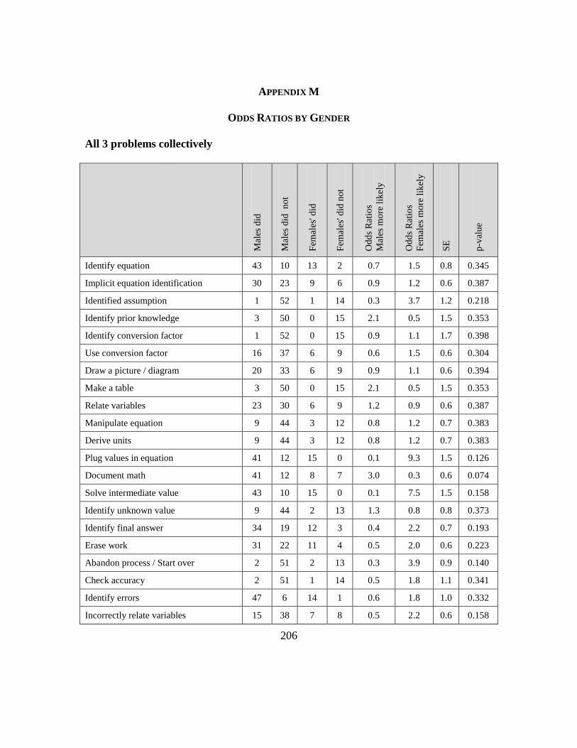
206

APPENDIX M

ODDS RATIOS BY GENDER

All 3 problems collectively

Mal

es d

id

Mal

es d

id

no

t

Fem

ales

' did

Fem

ales

' did

no

t

Od

ds

Rat

ios

Mal

es m

ore

lik

ely

Od

ds

Rat

ios

Fem

ales

mo

re l

ikel

y

SE

p-v

alu

e

Identify equation 43 10 13 2 0.7 1.5 0.8 0.345

Implicit equation identification 30 23 9 6 0.9 1.2 0.6 0.387

Identified assumption 1 52 1 14 0.3 3.7 1.2 0.218

Identify prior knowledge 3 50 0 15 2.1 0.5 1.5 0.353

Identify conversion factor 1 52 0 15 0.9 1.1 1.7 0.398

Use conversion factor 16 37 6 9 0.6 1.5 0.6 0.304

Draw a picture / diagram 20 33 6 9 0.9 1.1 0.6 0.394

Make a table 3 50 0 15 2.1 0.5 1.5 0.353

Relate variables 23 30 6 9 1.2 0.9 0.6 0.387

Manipulate equation 9 44 3 12 0.8 1.2 0.7 0.383

Derive units 9 44 3 12 0.8 1.2 0.7 0.383

Plug values in equation 41 12 15 0 0.1 9.3 1.5 0.126

Document math 41 12 8 7 3.0 0.3 0.6 0.074

Solve intermediate value 43 10 15 0 0.1 7.5 1.5 0.158

Identify unknown value 9 44 2 13 1.3 0.8 0.8 0.373

Identify final answer 34 19 12 3 0.4 2.2 0.7 0.193

Erase work 31 22 11 4 0.5 2.0 0.6 0.223

Abandon process / Start over 2 51 2 13 0.3 3.9 0.9 0.140

Check accuracy 2 51 1 14 0.5 1.8 1.1 0.341

Identify errors 47 6 14 1 0.6 1.8 1.0 0.332

Incorrectly relate variables 15 38 7 8 0.5 2.2 0.6 0.158

207

Misuse governing equation 11 42 6 9 0.4 2.5 0.6 0.122

Incorrect visual/graphic representation 1 52 0 15 0.9 1.1 1.7 0.398

Incorrect assumptions 0 53 1 14 0.1 11.1 1.7 0.140

Incorrectly manipulate equation 1 52 0 15 0.9 1.1 1.7 0.398

Incorrect calculation 6 47 4 11 0.4 2.8 0.7 0.129

Incorrect unit derivation 2 51 3 12 0.2 6.4 0.9 0.045

Incorrect known value 5 48 3 12 0.4 2.4 0.8 0.203

Incorrect unknown value 3 50 2 13 0.4 2.6 0.9 0.226

Ignored problem constraints 6 47 2 13 0.8 1.2 0.8 0.388

Irrelevant information 9 44 4 11 0.6 1.8 0.7 0.273

Inconsistent transcription 3 50 3 12 0.2 4.2 0.8 0.088

Inconsistent units 15 38 3 12 1.6 0.6 0.7 0.317

Incorrect unit assignment 4 49 1 14 1.1 0.9 1.0 0.395

Using incorrectly generated information 10 43 6 9 0.3 2.9 0.6 0.092

Missing Units Throughout 2 51 0 15 1.5 0.7 1.6 0.386

Erasing correct work 16 37 6 9 0.6 1.5 0.6 0.304

Plug and chug 12 41 7 8 0.3 3.0 0.6 0.074

Guess and Check 6 47 5 10 0.3 3.9 0.7 0.051

Segmentation 17 36 4 11 1.3 0.8 0.6 0.366

Means-ends analysis 9 44 0 15 6.6 0.2 1.5 0.177

Chunking 16 37 1 14 6.1 0.2 0.9 0.056

Forward chaining 7 46 2 13 1.0 1.0 0.8 0.399

Correct Answer 34 19 2 13 11.6 0.1 0.7 0.002

Correct but Incorrect Units 4 49 1 14 1.1 0.9 1.0 0.395

Incorrect Answer 32 21 12 3 0.4 2.6 0.7 0.139

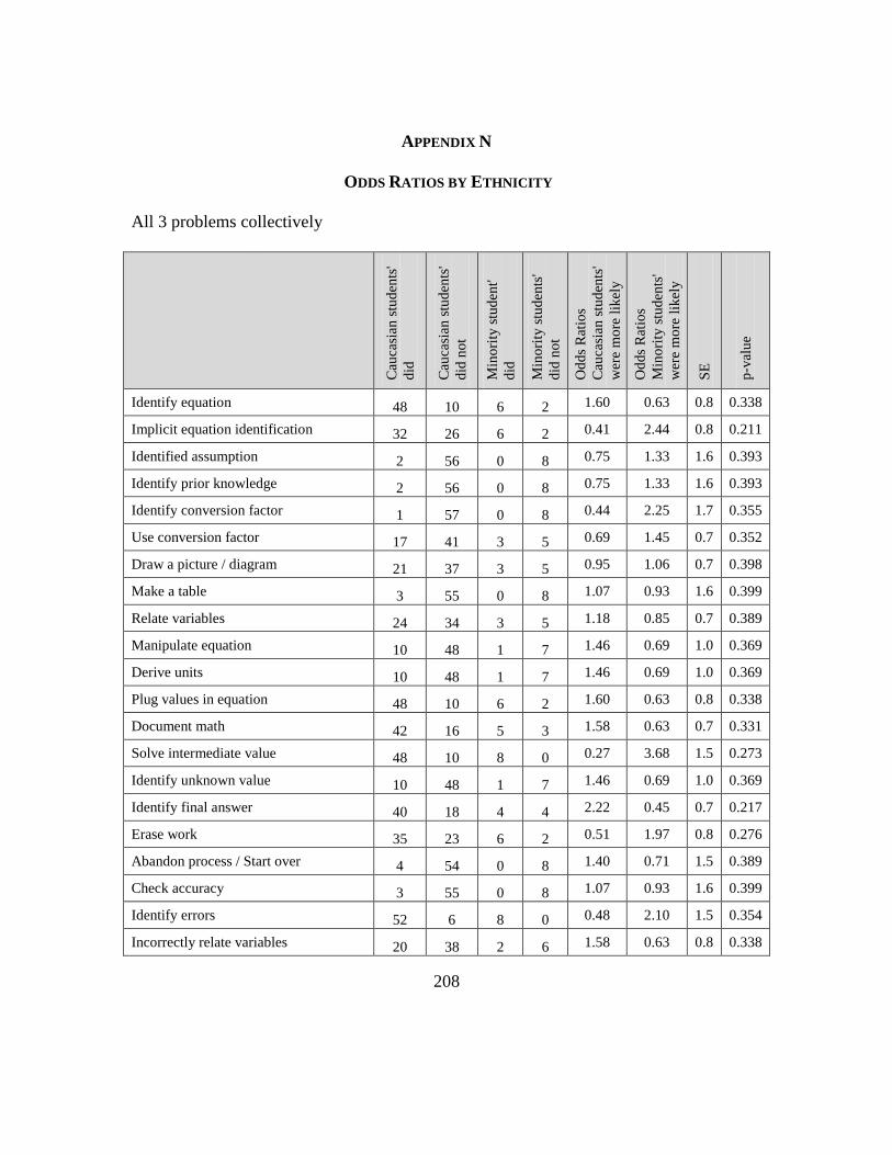
208

APPENDIX N

ODDS RATIOS BY ETHNICITY

All 3 problems collectively

Cau

casi

an s

tud

ents

'

did

Cau

casi

an s

tud

ents

'

did

no

t

Min

ori

ty s

tud

ent'

did

Min

ori

ty s

tud

ents

'

did

no

t

Od

ds

Rat

ios

Cau

casi

an s

tud

ents

'

wer

e m

ore

lik

ely

Od

ds

Rat

ios

Min

ori

ty s

tud

ents

'

wer

e m

ore

lik

ely

SE

p-v

alu

e

Identify equation 48 10 6 2 1.60 0.63 0.8 0.338

Implicit equation identification 32 26 6 2 0.41 2.44 0.8 0.211

Identified assumption 2 56 0 8 0.75 1.33 1.6 0.393

Identify prior knowledge 2 56 0 8 0.75 1.33 1.6 0.393

Identify conversion factor 1 57 0 8 0.44 2.25 1.7 0.355

Use conversion factor 17 41 3 5 0.69 1.45 0.7 0.352

Draw a picture / diagram 21 37 3 5 0.95 1.06 0.7 0.398

Make a table 3 55 0 8 1.07 0.93 1.6 0.399

Relate variables 24 34 3 5 1.18 0.85 0.7 0.389

Manipulate equation 10 48 1 7 1.46 0.69 1.0 0.369

Derive units 10 48 1 7 1.46 0.69 1.0 0.369

Plug values in equation 48 10 6 2 1.60 0.63 0.8 0.338

Document math 42 16 5 3 1.58 0.63 0.7 0.331

Solve intermediate value 48 10 8 0 0.27 3.68 1.5 0.273

Identify unknown value 10 48 1 7 1.46 0.69 1.0 0.369

Identify final answer 40 18 4 4 2.22 0.45 0.7 0.217

Erase work 35 23 6 2 0.51 1.97 0.8 0.276

Abandon process / Start over 4 54 0 8 1.40 0.71 1.5 0.389

Check accuracy 3 55 0 8 1.07 0.93 1.6 0.399

Identify errors 52 6 8 0 0.48 2.10 1.5 0.354

Incorrectly relate variables 20 38 2 6 1.58 0.63 0.8 0.338

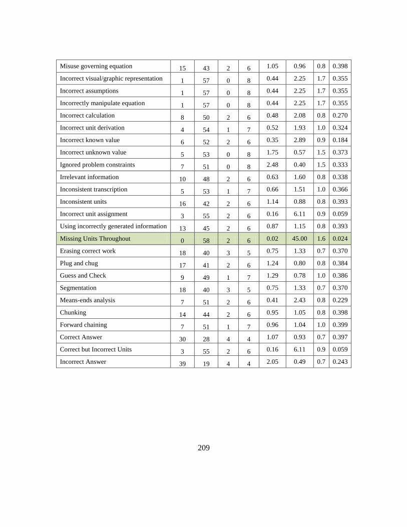
209

Misuse governing equation 15 43 2 6 1.05 0.96 0.8 0.398

Incorrect visual/graphic representation 1 57 0 8 0.44 2.25 1.7 0.355

Incorrect assumptions 1 57 0 8 0.44 2.25 1.7 0.355

Incorrectly manipulate equation 1 57 0 8 0.44 2.25 1.7 0.355

Incorrect calculation 8 50 2 6 0.48 2.08 0.8 0.270

Incorrect unit derivation 4 54 1 7 0.52 1.93 1.0 0.324

Incorrect known value 6 52 2 6 0.35 2.89 0.9 0.184

Incorrect unknown value 5 53 0 8 1.75 0.57 1.5 0.373

Ignored problem constraints 7 51 0 8 2.48 0.40 1.5 0.333

Irrelevant information 10 48 2 6 0.63 1.60 0.8 0.338

Inconsistent transcription 5 53 1 7 0.66 1.51 1.0 0.366

Inconsistent units 16 42 2 6 1.14 0.88 0.8 0.393

Incorrect unit assignment 3 55 2 6 0.16 6.11 0.9 0.059

Using incorrectly generated information 13 45 2 6 0.87 1.15 0.8 0.393

Missing Units Throughout 0 58 2 6 0.02 45.00 1.6 0.024

Erasing correct work 18 40 3 5 0.75 1.33 0.7 0.370

Plug and chug 17 41 2 6 1.24 0.80 0.8 0.384

Guess and Check 9 49 1 7 1.29 0.78 1.0 0.386

Segmentation 18 40 3 5 0.75 1.33 0.7 0.370

Means-ends analysis 7 51 2 6 0.41 2.43 0.8 0.229

Chunking 14 44 2 6 0.95 1.05 0.8 0.398

Forward chaining 7 51 1 7 0.96 1.04 1.0 0.399

Correct Answer 30 28 4 4 1.07 0.93 0.7 0.397

Correct but Incorrect Units 3 55 2 6 0.16 6.11 0.9 0.059

Incorrect Answer 39 19 4 4 2.05 0.49 0.7 0.243

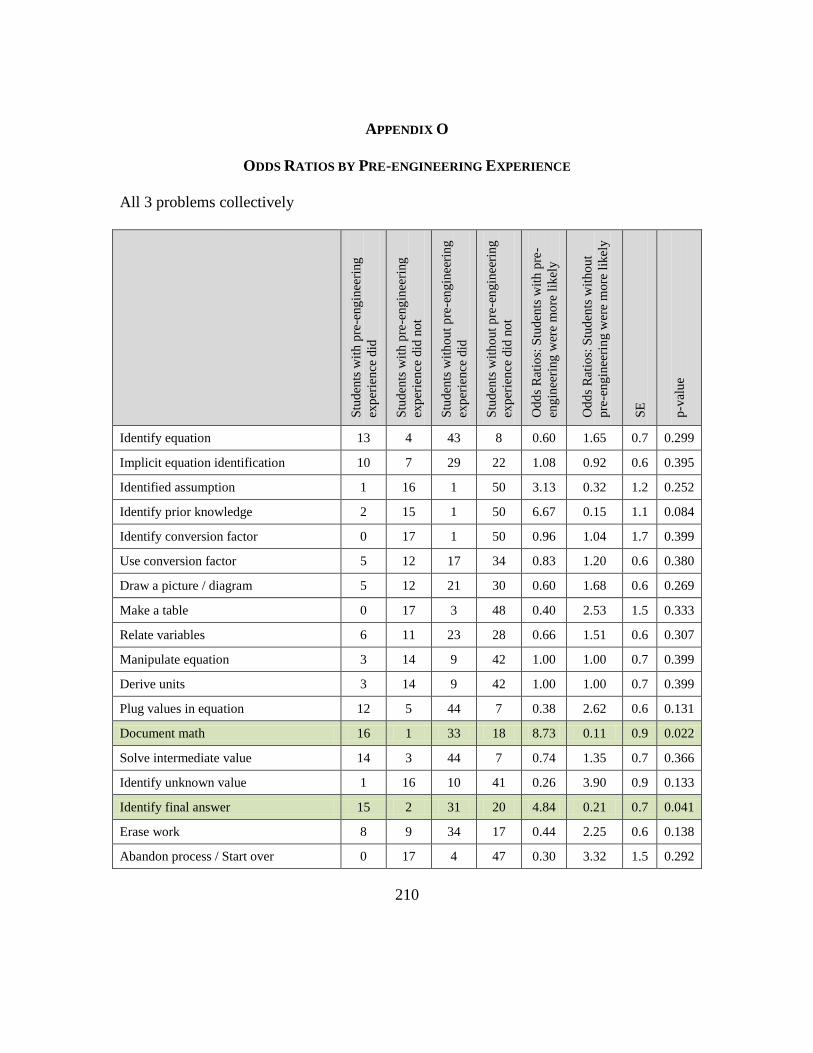
210

APPENDIX O

ODDS RATIOS BY PRE-ENGINEERING EXPERIENCE

All 3 problems collectively

Stu

den

ts w

ith

pre

-eng

inee

ring

exp

erie

nce

did

Stu

den

ts w

ith

pre

-eng

inee

ring

exp

erie

nce

did

no

t

Stu

den

ts w

ith

ou

t p

re-e

ng

inee

rin

g

exp

erie

nce

did

Stu

den

ts w

ith

ou

t p

re-e

ng

inee

rin

g

exp

erie

nce

did

no

t

Od

ds

Rat

ios:

Stu

den

ts w

ith

pre

-

eng

inee

ring

wer

e m

ore

lik

ely

Od

ds

Rat

ios:

Stu

den

ts w

ith

ou

t

pre

-eng

inee

rin

g w

ere

more

lik

ely

SE

p-v

alu

e

Identify equation 13 4 43 8 0.60 1.65 0.7 0.299

Implicit equation identification 10 7 29 22 1.08 0.92 0.6 0.395

Identified assumption 1 16 1 50 3.13 0.32 1.2 0.252

Identify prior knowledge 2 15 1 50 6.67 0.15 1.1 0.084

Identify conversion factor 0 17 1 50 0.96 1.04 1.7 0.399

Use conversion factor 5 12 17 34 0.83 1.20 0.6 0.380

Draw a picture / diagram 5 12 21 30 0.60 1.68 0.6 0.269

Make a table 0 17 3 48 0.40 2.53 1.5 0.333

Relate variables 6 11 23 28 0.66 1.51 0.6 0.307

Manipulate equation 3 14 9 42 1.00 1.00 0.7 0.399

Derive units 3 14 9 42 1.00 1.00 0.7 0.399

Plug values in equation 12 5 44 7 0.38 2.62 0.6 0.131

Document math 16 1 33 18 8.73 0.11 0.9 0.022

Solve intermediate value 14 3 44 7 0.74 1.35 0.7 0.366

Identify unknown value 1 16 10 41 0.26 3.90 0.9 0.133

Identify final answer 15 2 31 20 4.84 0.21 0.7 0.041

Erase work 8 9 34 17 0.44 2.25 0.6 0.138

Abandon process / Start over 0 17 4 47 0.30 3.32 1.5 0.292

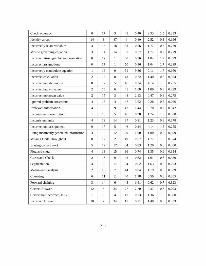
211

Check accuracy 0 17 3 48 0.40 2.53 1.5 0.333

Identify errors 14 3 47 4 0.40 2.52 0.8 0.196

Incorrectly relate variables 4 13 18 33 0.56 1.77 0.6 0.259

Misuse governing equation 3 14 14 37 0.57 1.77 0.7 0.279

Incorrect visual/graphic representation 0 17 1 50 0.96 1.04 1.7 0.399

Incorrect assumptions 0 17 1 50 0.96 1.04 1.7 0.399

Incorrectly manipulate equation 1 16 0 51 9.36 0.11 1.7 0.160

Incorrect calculation 2 15 8 43 0.72 1.40 0.8 0.364

Incorrect unit derivation 0 17 5 46 0.24 4.14 1.5 0.255

Incorrect known value 2 15 6 45 1.00 1.00 0.8 0.399

Incorrect unknown value 2 15 3 48 2.13 0.47 0.9 0.275

Ignored problem constraints 4 13 4 47 3.62 0.28 0.7 0.086

Irrelevant information 4 13 9 42 1.44 0.70 0.7 0.342

Inconsistent transcription 1 16 5 46 0.58 1.74 1.0 0.338

Inconsistent units 4 13 14 37 0.81 1.23 0.6 0.378

Incorrect unit assignment 0 17 5 46 0.24 4.14 1.5 0.255

Using incorrectly generated information 4 13 12 39 1.00 1.00 0.6 0.399

Missing Units Throughout 0 17 2 49 0.57 1.77 1.6 0.374

Erasing correct work 5 12 17 34 0.83 1.20 0.6 0.380

Plug and chug 4 13 15 36 0.74 1.35 0.6 0.354

Guess and Check 2 15 9 42 0.62 1.61 0.8 0.330

Segmentation 4 13 17 34 0.62 1.63 0.6 0.293

Means-ends analysis 2 15 7 44 0.84 1.19 0.8 0.389

Chunking 6 11 11 40 1.98 0.50 0.6 0.205

Forward chaining 3 14 6 45 1.61 0.62 0.7 0.323

Correct Answer 12 5 24 27 2.70 0.37 0.6 0.093

Correct but Incorrect Units 1 16 4 47 0.73 1.36 1.0 0.380

Incorrect Answer 10 7 34 17 0.71 1.40 0.6 0.333

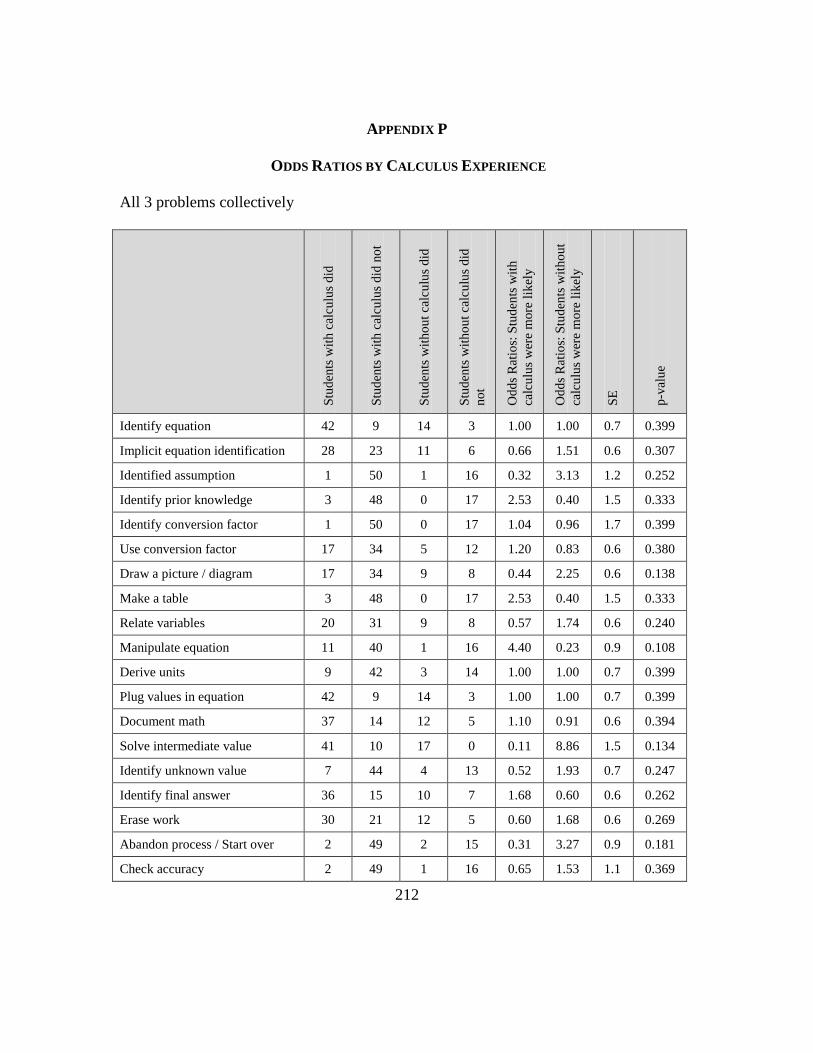
212

APPENDIX P

ODDS RATIOS BY CALCULUS EXPERIENCE

All 3 problems collectively S

tud

ents

wit

h c

alcu

lus

did

Stu

den

ts w

ith

cal

culu

s d

id n

ot

Stu

den

ts w

ith

ou

t ca

lcu

lus

did

Stu

den

ts w

ith

ou

t ca

lcu

lus

did

no

t

Od

ds

Rat

ios:

Stu

den

ts w

ith

calc

ulu

s w

ere

mo

re l

ikel

y

Od

ds

Rat

ios:

Stu

den

ts w

ith

ou

t

calc

ulu

s w

ere

mo

re l

ikel

y

SE

p-v

alu

e

Identify equation 42 9 14 3 1.00 1.00 0.7 0.399

Implicit equation identification 28 23 11 6 0.66 1.51 0.6 0.307

Identified assumption 1 50 1 16 0.32 3.13 1.2 0.252

Identify prior knowledge 3 48 0 17 2.53 0.40 1.5 0.333

Identify conversion factor 1 50 0 17 1.04 0.96 1.7 0.399

Use conversion factor 17 34 5 12 1.20 0.83 0.6 0.380

Draw a picture / diagram 17 34 9 8 0.44 2.25 0.6 0.138

Make a table 3 48 0 17 2.53 0.40 1.5 0.333

Relate variables 20 31 9 8 0.57 1.74 0.6 0.240

Manipulate equation 11 40 1 16 4.40 0.23 0.9 0.108

Derive units 9 42 3 14 1.00 1.00 0.7 0.399

Plug values in equation 42 9 14 3 1.00 1.00 0.7 0.399

Document math 37 14 12 5 1.10 0.91 0.6 0.394

Solve intermediate value 41 10 17 0 0.11 8.86 1.5 0.134

Identify unknown value 7 44 4 13 0.52 1.93 0.7 0.247

Identify final answer 36 15 10 7 1.68 0.60 0.6 0.262

Erase work 30 21 12 5 0.60 1.68 0.6 0.269

Abandon process / Start over 2 49 2 15 0.31 3.27 0.9 0.181

Check accuracy 2 49 1 16 0.65 1.53 1.1 0.369

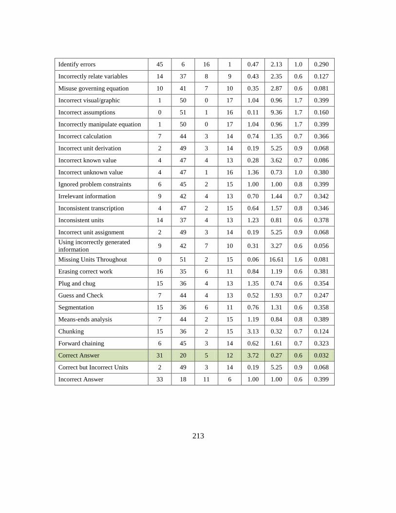
213

Identify errors 45 6 16 1 0.47 2.13 1.0 0.290

Incorrectly relate variables 14 37 8 9 0.43 2.35 0.6 0.127

Misuse governing equation 10 41 7 10 0.35 2.87 0.6 0.081

Incorrect visual/graphic 1 50 0 17 1.04 0.96 1.7 0.399

Incorrect assumptions 0 51 1 16 0.11 9.36 1.7 0.160

Incorrectly manipulate equation 1 50 0 17 1.04 0.96 1.7 0.399

Incorrect calculation 7 44 3 14 0.74 1.35 0.7 0.366

Incorrect unit derivation 2 49 3 14 0.19 5.25 0.9 0.068

Incorrect known value 4 47 4 13 0.28 3.62 0.7 0.086

Incorrect unknown value 4 47 1 16 1.36 0.73 1.0 0.380

Ignored problem constraints 6 45 2 15 1.00 1.00 0.8 0.399

Irrelevant information 9 42 4 13 0.70 1.44 0.7 0.342

Inconsistent transcription 4 47 2 15 0.64 1.57 0.8 0.346

Inconsistent units 14 37 4 13 1.23 0.81 0.6 0.378

Incorrect unit assignment 2 49 3 14 0.19 5.25 0.9 0.068

Using incorrectly generated

information 9 42 7 10 0.31 3.27 0.6 0.056

Missing Units Throughout 0 51 2 15 0.06 16.61 1.6 0.081

Erasing correct work 16 35 6 11 0.84 1.19 0.6 0.381

Plug and chug 15 36 4 13 1.35 0.74 0.6 0.354

Guess and Check 7 44 4 13 0.52 1.93 0.7 0.247

Segmentation 15 36 6 11 0.76 1.31 0.6 0.358

Means-ends analysis 7 44 2 15 1.19 0.84 0.8 0.389

Chunking 15 36 2 15 3.13 0.32 0.7 0.124

Forward chaining 6 45 3 14 0.62 1.61 0.7 0.323

Correct Answer 31 20 5 12 3.72 0.27 0.6 0.032

Correct but Incorrect Units 2 49 3 14 0.19 5.25 0.9 0.068

Incorrect Answer 33 18 11 6 1.00 1.00 0.6 0.399

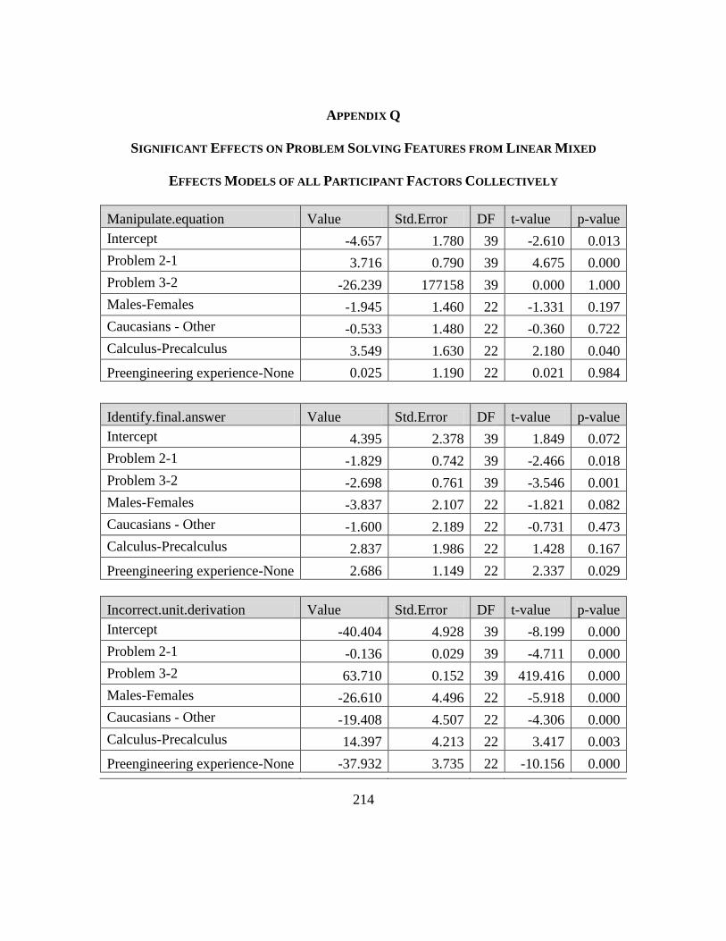
214

APPENDIX Q

SIGNIFICANT EFFECTS ON PROBLEM SOLVING FEATURES FROM LINEAR MIXED

EFFECTS MODELS OF ALL PARTICIPANT FACTORS COLLECTIVELY

Manipulate.equation Value Std.Error DF t-value p-value

Intercept -4.657 1.780 39 -2.610 0.013

Problem 2-1 3.716 0.790 39 4.675 0.000

Problem 3-2 -26.239 177158 39 0.000 1.000

Males-Females -1.945 1.460 22 -1.331 0.197

Caucasians - Other -0.533 1.480 22 -0.360 0.722

Calculus-Precalculus 3.549 1.630 22 2.180 0.040

Preengineering experience-None 0.025 1.190 22 0.021 0.984

Identify.final.answer Value Std.Error DF t-value p-value

Intercept 4.395 2.378 39 1.849 0.072

Problem 2-1 -1.829 0.742 39 -2.466 0.018

Problem 3-2 -2.698 0.761 39 -3.546 0.001

Males-Females -3.837 2.107 22 -1.821 0.082

Caucasians - Other -1.600 2.189 22 -0.731 0.473

Calculus-Precalculus 2.837 1.986 22 1.428 0.167

Preengineering experience-None 2.686 1.149 22 2.337 0.029

Incorrect.unit.derivation Value Std.Error DF t-value p-value

Intercept -40.404 4.928 39 -8.199 0.000

Problem 2-1 -0.136 0.029 39 -4.711 0.000

Problem 3-2 63.710 0.152 39 419.416 0.000

Males-Females -26.610 4.496 22 -5.918 0.000

Caucasians - Other -19.408 4.507 22 -4.306 0.000

Calculus-Precalculus 14.397 4.213 22 3.417 0.003

Preengineering experience-None -37.932 3.735 22 -10.156 0.000

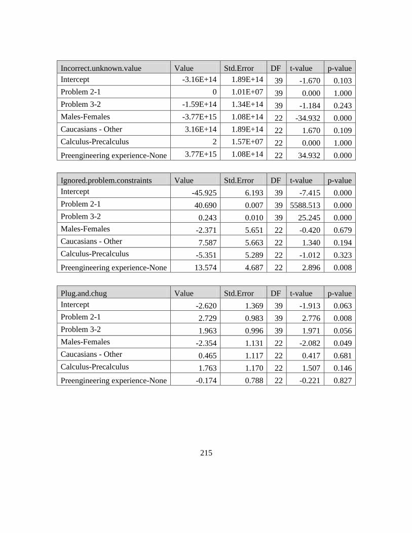
215

Incorrect.unknown.value Value Std.Error DF t-value p-value

Intercept -3.16E+14 1.89E+14 39 -1.670 0.103

Problem 2-1 0 1.01E+07 39 0.000 1.000

Problem 3-2 -1.59E+14 1.34E+14 39 -1.184 0.243

Males-Females -3.77E+15 1.08E+14 22 -34.932 0.000

Caucasians - Other 3.16E+14 1.89E+14 22 1.670 0.109

Calculus-Precalculus 2 1.57E+07 22 0.000 1.000

Preengineering experience-None 3.77E+15 1.08E+14 22 34.932 0.000

Ignored.problem.constraints Value Std.Error DF t-value p-value

Intercept -45.925 6.193 39 -7.415 0.000

Problem 2-1 40.690 0.007 39 5588.513 0.000

Problem 3-2 0.243 0.010 39 25.245 0.000

Males-Females -2.371 5.651 22 -0.420 0.679

Caucasians - Other 7.587 5.663 22 1.340 0.194

Calculus-Precalculus -5.351 5.289 22 -1.012 0.323

Preengineering experience-None 13.574 4.687 22 2.896 0.008

Plug.and.chug Value Std.Error DF t-value p-value

Intercept -2.620 1.369 39 -1.913 0.063

Problem 2-1 2.729 0.983 39 2.776 0.008

Problem 3-2 1.963 0.996 39 1.971 0.056

Males-Females -2.354 1.131 22 -2.082 0.049

Caucasians - Other 0.465 1.117 22 0.417 0.681

Calculus-Precalculus 1.763 1.170 22 1.507 0.146

Preengineering experience-None -0.174 0.788 22 -0.221 0.827

216

Means.ends.analysis Value Std.Error DF t-value p-value

Intercept -103.712 5.860 39 -17.698 0.000

Problem 2-1 6.832 0.299 39 22.811 0.000

Problem 3-2 65.298 0.298 39 218.802 0.000

Males-Females 63.837 5.345 22 11.944 0.000

Caucasians - Other 12.851 5.354 22 2.400 0.025

Calculus-Precalculus -37.293 5.000 22 -7.458 0.000

Preengineering experience-None -4.877 4.424 22 -1.102 0.282

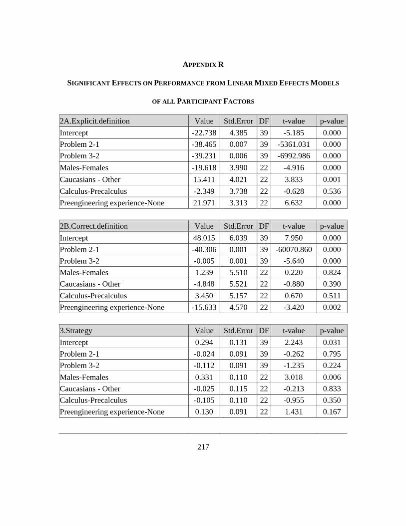
217

APPENDIX R

SIGNIFICANT EFFECTS ON PERFORMANCE FROM LINEAR MIXED EFFECTS MODELS

OF ALL PARTICIPANT FACTORS

2A.Explicit.definition Value Std.Error DF t-value p-value

Intercept -22.738 4.385 39 -5.185 0.000

Problem 2-1 -38.465 0.007 39 -5361.031 0.000

Problem 3-2 -39.231 0.006 39 -6992.986 0.000

Males-Females -19.618 3.990 22 -4.916 0.000

Caucasians - Other 15.411 4.021 22 3.833 0.001

Calculus-Precalculus -2.349 3.738 22 -0.628 0.536

Preengineering experience-None 21.971 3.313 22 6.632 0.000

2B.Correct.definition Value Std.Error DF t-value p-value

Intercept 48.015 6.039 39 7.950 0.000

Problem 2-1 -40.306 0.001 39 -60070.860 0.000

Problem 3-2 -0.005 0.001 39 -5.640 0.000

Males-Females 1.239 5.510 22 0.220 0.824

Caucasians - Other -4.848 5.521 22 -0.880 0.390

Calculus-Precalculus 3.450 5.157 22 0.670 0.511

Preengineering experience-None -15.633 4.570 22 -3.420 0.002

3.Strategy Value Std.Error DF t-value p-value

Intercept 0.294 0.131 39 2.243 0.031

Problem 2-1 -0.024 0.091 39 -0.262 0.795

Problem 3-2 -0.112 0.091 39 -1.235 0.224

Males-Females 0.331 0.110 22 3.018 0.006

Caucasians - Other -0.025 0.115 22 -0.213 0.833

Calculus-Precalculus -0.105 0.110 22 -0.955 0.350

Preengineering experience-None 0.130 0.091 22 1.431 0.167

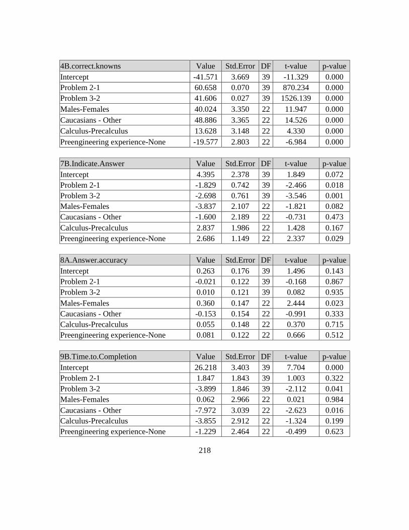
218

4B.correct.knowns Value Std.Error DF t-value p-value

Intercept -41.571 3.669 39 -11.329 0.000

Problem 2-1 60.658 0.070 39 870.234 0.000

Problem 3-2 41.606 0.027 39 1526.139 0.000

Males-Females 40.024 3.350 22 11.947 0.000

Caucasians - Other 48.886 3.365 22 14.526 0.000

Calculus-Precalculus 13.628 3.148 22 4.330 0.000

Preengineering experience-None -19.577 2.803 22 -6.984 0.000

7B.Indicate.Answer Value Std.Error DF t-value p-value

Intercept 4.395 2.378 39 1.849 0.072

Problem 2-1 -1.829 0.742 39 -2.466 0.018

Problem 3-2 -2.698 0.761 39 -3.546 0.001

Males-Females -3.837 2.107 22 -1.821 0.082

Caucasians - Other -1.600 2.189 22 -0.731 0.473

Calculus-Precalculus 2.837 1.986 22 1.428 0.167

Preengineering experience-None 2.686 1.149 22 2.337 0.029

8A.Answer.accuracy Value Std.Error DF t-value p-value

Intercept 0.263 0.176 39 1.496 0.143

Problem 2-1 -0.021 0.122 39 -0.168 0.867

Problem 3-2 0.010 0.121 39 0.082 0.935

Males-Females 0.360 0.147 22 2.444 0.023

Caucasians - Other -0.153 0.154 22 -0.991 0.333

Calculus-Precalculus 0.055 0.148 22 0.370 0.715

Preengineering experience-None 0.081 0.122 22 0.666 0.512

9B.Time.to.Completion Value Std.Error DF t-value p-value

Intercept 26.218 3.403 39 7.704 0.000

Problem 2-1 1.847 1.843 39 1.003 0.322

Problem 3-2 -3.899 1.846 39 -2.112 0.041

Males-Females 0.062 2.966 22 0.021 0.984

Caucasians - Other -7.972 3.039 22 -2.623 0.016

Calculus-Precalculus -3.855 2.912 22 -1.324 0.199

Preengineering experience-None -1.229 2.464 22 -0.499 0.623

219

APPENDIX S

SIGNIFICANT RELATIONSHIPS BETWEEN PROCESS AND OUTCOME MEASURES FROM

LINEAR MIXED EFFECTS MODELS

X8A.Answer.accuracy

Value Std.Error DF t-value p-value

Intercept 0.429 0.064 78 6.691 0.000

Problem 2-1 -0.033 0.068 78 -0.488 0.627

Problem 3-2 0.010 0.066 78 0.158 0.875

Semester Spring 2011-Fall 2009 0.384 0.069 61 5.548 0.000

X2E.correct.representation 0.141 0.062 78 2.284 0.025

X8A.Answer.accuracy

Value Std.Error DF t-value p-value

Intercept 0.230 0.070 78 3.278 0.002

Problem 2-1 0.017 0.066 78 0.263 0.793

Problem 3-2 0.022 0.065 78 0.336 0.738

Semester Spring 2011-Fall 2009 0.407 0.057 61 7.112 0.000

X3.Strategy 0.514 0.095 78 5.425 0.000

X8A.Answer.accuracy

Value Std.Error DF t-value p-value

Intercept 0.424 0.065 78 6.556 0.000

Problem 2-1 0.001 0.066 78 0.016 0.987

Problem 3-2 0.049 0.065 78 0.752 0.454

Semester Spring 2011-Fall 2009 0.406 0.071 61 5.741 0.000

X4D.NumHitKnowns 0.230 0.085 78 2.698 0.009

X8A.Answer.accuracy

Value Std.Error DF t-value p-value

Intercept 0.191 0.122 78 1.563 0.122

Problem 2-1 0.019 0.068 78 0.283 0.778

Problem 3-2 0.047 0.067 78 0.699 0.487

Semester Spring 2011-Fall 2009 0.383 0.067 61 5.669 0.000

X5B.correct.mechanical 0.288 0.111 78 2.586 0.012

220

X8A.Answer.accuracy

Value Std.Error DF t-value p-value

Intercept -0.401 0.141 78 -2.848 0.006

Problem 2-1 0.045 0.060 78 0.747 0.457

Problem 3-2 0.052 0.059 78 0.888 0.378

Semester Spring 2011-Fall 2009 0.322 0.062 61 5.196 0.000

X6A.Sensitivity 1.054 0.158 78 6.666 0.000

X8A.Answer.accuracy

Value Std.Error DF t-value p-value

Intercept 0.155 0.066 78 2.343 0.022

Problem 2-1 0.071 0.058 78 1.230 0.222

Problem 3-2 0.060 0.056 78 1.075 0.286

Semester Spring 2011-Fall 2009 0.307 0.060 61 5.144 0.000

X6B.Hit.Rate 0.563 0.072 78 7.843 0.000

X8B.Conceptual.Errors

Value Std.Error DF t-value p-value

Intercept 0.819 0.100 78 8.177 0.000

Problem 2-1 -0.347 0.120 78 -2.901 0.005

Problem 3-2 -0.514 0.116 78 -4.422 0.000

Semester Spring 2011-Fall 2009 -0.103 0.100 61 -1.026 0.309

X2E.correct.representation -0.351 0.102 78 -3.452 0.001

X8B.Conceptual.Errors

Value Std.Error DF t-value p-value

Intercept 1.240 0.179 78 6.944 0.000

Problem 2-1 -0.347 0.118 78 -2.938 0.004

Problem 3-2 -0.464 0.117 78 -3.970 0.000

Semester Spring 2011-Fall 2009 -0.208 0.104 61 -2.008 0.049

X4B.correct.knowns -0.577 0.170 78 -3.390 0.001

X8B.Conceptual.Errors

Value Std.Error DF t-value p-value

Intercept 1.768 0.156 78 11.359 0.000

Problem 2-1 -0.480 0.104 78 -4.608 0.000

Problem 3-2 -0.486 0.102 78 -4.763 0.000

Semester Spring 2011-Fall 2009 -0.177 0.084 61 -2.098 0.040

X4C.correct.equations -1.128 0.144 78 -7.837 0.000

221

X8B.Conceptual.Errors

Value Std.Error DF t-value p-value

Intercept 1.554 0.262 78 5.942 0.000

Problem 2-1 -0.467 0.121 78 -3.865 0.000

Problem 3-2 -0.580 0.118 78 -4.932 0.000

Semester Spring 2011-Fall 2009 -0.072 0.101 61 -0.720 0.475

X6A.Sensitivity -0.995 0.297 78 -3.349 0.001

X8B.Conceptual.Errors

Value Std.Error DF t-value p-value

Intercept 1.093 0.119 78 9.190 0.000

Problem 2-1 -0.507 0.117 78 -4.333 0.000

Problem 3-2 -0.595 0.113 78 -5.248 0.000

Semester Spring 2011-Fall 2009 -0.034 0.097 61 -0.352 0.726

X6B.Hit.Rate -0.653 0.136 78 -4.782 0.000

X8C.Mechanical.Errors

Value Std.Error DF t-value p-value

Intercept 1.174 0.037 78 31.436 0.000

Problem 2-1 0.006 0.022 78 0.269 0.788

Problem 3-2 0.005 0.022 78 0.226 0.822

Semester Spring 2011-Fall 2009 0.013 0.019 61 0.695 0.490

X5B.correct.mechanical -1.184 0.035 78 -34.072 0.000

X8C.Mechanical.Errors

Value Std.Error DF t-value p-value

Intercept 0.149 0.069 78 2.156 0.034

Problem 2-1 0.090 0.068 78 1.332 0.187

Problem 3-2 0.095 0.066 78 1.439 0.154

Semester Spring 2011-Fall 2009 -0.051 0.056 61 -0.907 0.368

X6B.Hit.Rate -0.161 0.079 78 -2.028 0.046

X8D.Management.Errors

Value Std.Error DF t-value p-value

Intercept 3.878 0.552 78 7.022 0.000

Problem 2-1 -0.905 0.295 78 -3.067 0.003

Problem 3-2 -0.030 0.270 78 -0.111 0.912

Semester Spring 2011-Fall 2009 0.162 0.240 61 0.677 0.501

X2B.Correct.definition -2.486 0.513 78 -4.844 0.000

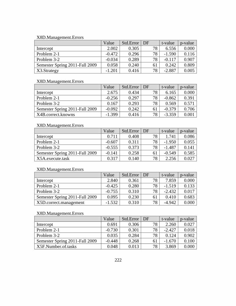
222

X8D.Management.Errors

Value Std.Error DF t-value p-value

Intercept 2.002 0.305 78 6.556 0.000

Problem 2-1 -0.472 0.296 78 -1.590 0.116

Problem 3-2 -0.034 0.289 78 -0.117 0.907

Semester Spring 2011-Fall 2009 0.058 0.240 61 0.242 0.809

X3.Strategy -1.201 0.416 78 -2.887 0.005

X8D.Management.Errors

Value Std.Error DF t-value p-value

Intercept 2.675 0.434 78 6.165 0.000

Problem 2-1 -0.256 0.297 78 -0.862 0.391

Problem 3-2 0.167 0.293 78 0.569 0.571

Semester Spring 2011-Fall 2009 -0.092 0.242 61 -0.379 0.706

X4B.correct.knowns -1.399 0.416 78 -3.359 0.001

X8D.Management.Errors

Value Std.Error DF t-value p-value

Intercept 0.711 0.408 78 1.741 0.086

Problem 2-1 -0.607 0.311 78 -1.950 0.055

Problem 3-2 -0.555 0.373 78 -1.487 0.141

Semester Spring 2011-Fall 2009 -0.141 0.258 61 -0.549 0.585

X5A.execute.task 0.317 0.140 78 2.256 0.027

X8D.Management.Errors

Value Std.Error DF t-value p-value

Intercept 2.840 0.361 78 7.859 0.000

Problem 2-1 -0.425 0.280 78 -1.519 0.133

Problem 3-2 -0.755 0.310 78 -2.432 0.017

Semester Spring 2011-Fall 2009 0.095 0.230 61 0.410 0.683

X5D.correct.management -1.532 0.310 78 -4.942 0.000

X8D.Management.Errors

Value Std.Error DF t-value p-value

Intercept 0.691 0.306 78 2.260 0.027

Problem 2-1 -0.730 0.301 78 -2.427 0.018

Problem 3-2 0.035 0.284 78 0.124 0.902

Semester Spring 2011-Fall 2009 -0.448 0.268 61 -1.670 0.100

X5F.Number.of.tasks 0.048 0.013 78 3.869 0.000

223

X8D.Management.Errors

Value Std.Error DF t-value p-value

Intercept 0.650 0.196 78 3.310 0.001

Problem 2-1 -0.095 0.227 78 -0.421 0.675

Problem 3-2 0.320 0.222 78 1.438 0.155

Semester Spring 2011-Fall 2009 0.109 0.183 61 0.597 0.553

X5G.Erasing.correct.work 1.209 0.112 78 10.775 0.000

X8D.Management.Errors

Value Std.Error DF t-value p-value

Intercept 3.696 0.634 78 5.831 0.000

Problem 2-1 -0.545 0.286 78 -1.902 0.061

Problem 3-2 -0.103 0.279 78 -0.369 0.713

Semester Spring 2011-Fall 2009 0.274 0.252 61 1.084 0.283

X6A.Sensitivity -2.747 0.718 78 -3.825 0.000

X8D.Management.Errors

Value Std.Error DF t-value p-value

Intercept 2.350 0.293 78 8.009 0.000

Problem 2-1 -0.635 0.276 78 -2.301 0.024

Problem 3-2 -0.133 0.267 78 -0.500 0.619

Semester Spring 2011-Fall 2009 0.348 0.250 61 1.389 0.170

X6B.Hit.Rate -1.665 0.331 78 -5.034 0.000

X8D.Management.Errors

Value Std.Error DF t-value p-value

Intercept 0.602 0.226 78 2.664 0.009

Problem 2-1 0.067 0.256 78 0.261 0.795

Problem 3-2 0.431 0.250 78 1.725 0.089

Semester Spring 2011-Fall 2009 0.178 0.203 61 0.877 0.384

X6C.False.Alarm.Rate 18.711 2.254 78 8.300 0.000

X9A.Error.Rate

Value Std.Error DF t-value p-value

Intercept 0.226 0.026 78 8.566 0.000

Problem 2-1 -0.018 0.025 78 -0.727 0.469

Problem 3-2 0.005 0.026 78 0.192 0.848

Semester Spring 2011-Fall 2009 -0.088 0.027 61 -3.229 0.002

X2F.NumRepHits 0.044 0.015 78 2.986 0.004

224

X9A.Error.Rate

Value Std.Error DF t-value p-value

Intercept 0.383 0.040 78 9.608 0.000

Problem 2-1 -0.053 0.023 78 -2.255 0.027

Problem 3-2 -0.024 0.023 78 -1.048 0.298

Semester Spring 2011-Fall 2009 -0.082 0.026 61 -3.108 0.003

X4C.correct.equations -0.133 0.035 78 -3.743 0.000

X9A.Error.Rate

Value Std.Error DF t-value p-value

Intercept 0.358 0.045 78 7.956 0.000

Problem 2-1 -0.054 0.024 78 -2.225 0.029

Problem 3-2 -0.040 0.024 78 -1.658 0.101

Semester Spring 2011-Fall 2009 -0.071 0.027 61 -2.663 0.010

X5B.correct.mechanical -0.102 0.041 78 -2.512 0.014

X9A.Error.Rate

Value Std.Error DF t-value p-value

Intercept 0.264 0.024 78 10.987 0.000

Problem 2-1 -0.050 0.024 78 -2.116 0.038

Problem 3-2 -0.049 0.024 78 -2.013 0.048

Semester Spring 2011-Fall 2009 -0.088 0.028 61 -3.174 0.002

X5C.Number.of.Times.

to.correct.mechanical 0.046 0.019 78 2.459 0.016

X9A.Error.Rate

Value Std.Error DF t-value p-value

Intercept 0.343 0.035 78 9.871 0.000

Problem 2-1 -0.043 0.023 78 -1.887 0.063

Problem 3-2 -0.073 0.026 78 -2.823 0.006

Semester Spring 2011-Fall 2009 -0.076 0.028 61 -2.696 0.009

X5D.correct.management -0.091 0.027 78 -3.307 0.001

X9A.Error.Rate

Value Std.Error DF t-value p-value

Intercept 0.261 0.024 78 10.899 0.000

Problem 2-1 -0.046 0.024 78 -1.972 0.052

Problem 3-2 -0.059 0.026 78 -2.303 0.024

Semester Spring 2011-Fall 2009 -0.082 0.027 61 -3.007 0.004

X5E.Number.of.Times.

to.correct.management 0.047 0.018 78 2.581 0.012

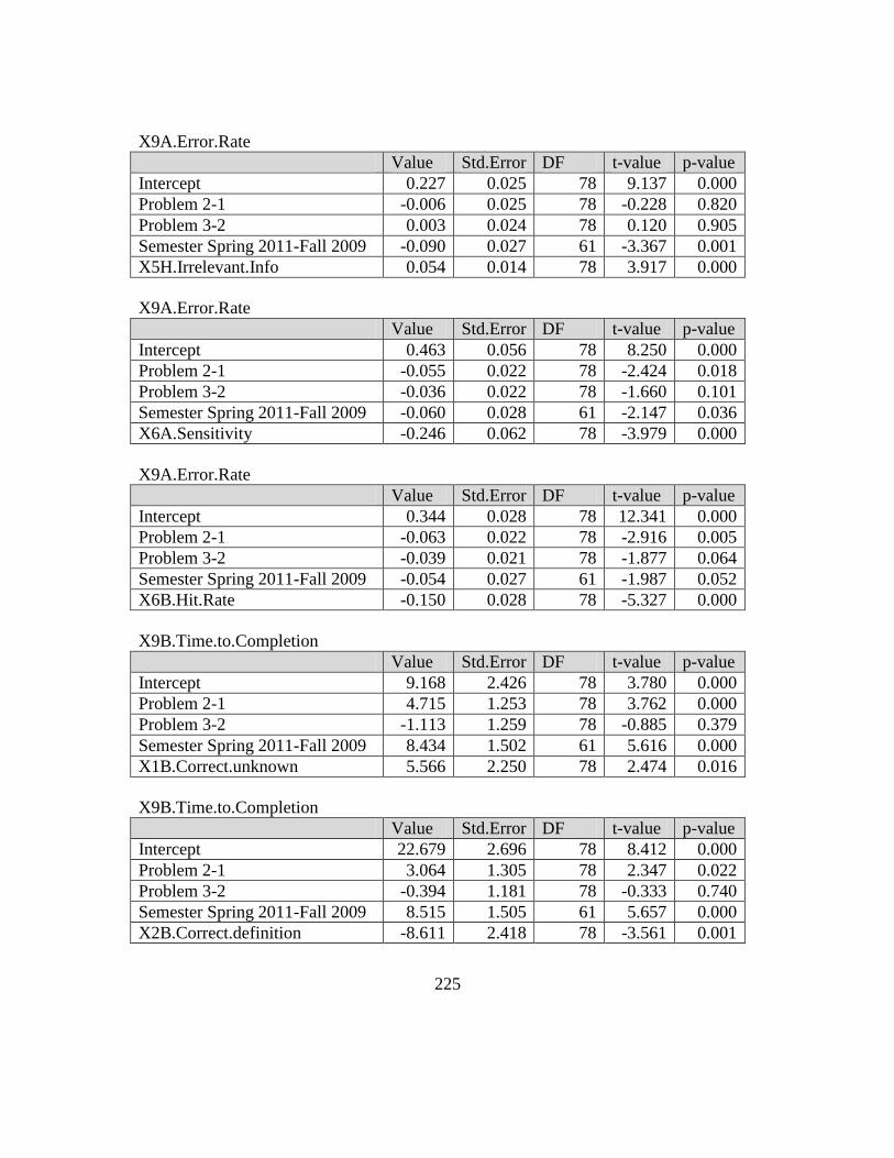
225

X9A.Error.Rate

Value Std.Error DF t-value p-value

Intercept 0.227 0.025 78 9.137 0.000

Problem 2-1 -0.006 0.025 78 -0.228 0.820

Problem 3-2 0.003 0.024 78 0.120 0.905

Semester Spring 2011-Fall 2009 -0.090 0.027 61 -3.367 0.001

X5H.Irrelevant.Info 0.054 0.014 78 3.917 0.000

X9A.Error.Rate

Value Std.Error DF t-value p-value

Intercept 0.463 0.056 78 8.250 0.000

Problem 2-1 -0.055 0.022 78 -2.424 0.018

Problem 3-2 -0.036 0.022 78 -1.660 0.101

Semester Spring 2011-Fall 2009 -0.060 0.028 61 -2.147 0.036

X6A.Sensitivity -0.246 0.062 78 -3.979 0.000

X9A.Error.Rate

Value Std.Error DF t-value p-value

Intercept 0.344 0.028 78 12.341 0.000

Problem 2-1 -0.063 0.022 78 -2.916 0.005

Problem 3-2 -0.039 0.021 78 -1.877 0.064

Semester Spring 2011-Fall 2009 -0.054 0.027 61 -1.987 0.052

X6B.Hit.Rate -0.150 0.028 78 -5.327 0.000

X9B.Time.to.Completion

Value Std.Error DF t-value p-value

Intercept 9.168 2.426 78 3.780 0.000

Problem 2-1 4.715 1.253 78 3.762 0.000

Problem 3-2 -1.113 1.259 78 -0.885 0.379

Semester Spring 2011-Fall 2009 8.434 1.502 61 5.616 0.000

X1B.Correct.unknown 5.566 2.250 78 2.474 0.016

X9B.Time.to.Completion

Value Std.Error DF t-value p-value

Intercept 22.679 2.696 78 8.412 0.000

Problem 2-1 3.064 1.305 78 2.347 0.022

Problem 3-2 -0.394 1.181 78 -0.333 0.740

Semester Spring 2011-Fall 2009 8.515 1.505 61 5.657 0.000

X2B.Correct.definition -8.611 2.418 78 -3.561 0.001

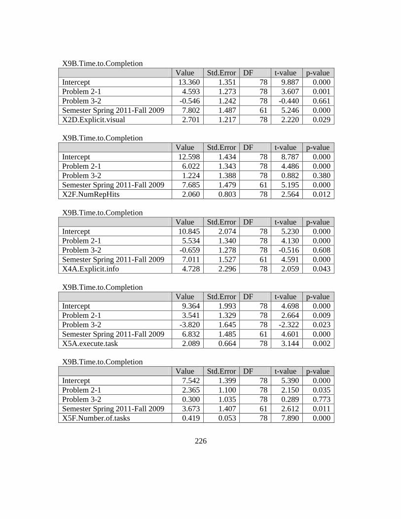
226

X9B.Time.to.Completion

Value Std.Error DF t-value p-value

Intercept 13.360 1.351 78 9.887 0.000

Problem 2-1 4.593 1.273 78 3.607 0.001

Problem 3-2 -0.546 1.242 78 -0.440 0.661

Semester Spring 2011-Fall 2009 7.802 1.487 61 5.246 0.000

X2D.Explicit.visual 2.701 1.217 78 2.220 0.029

X9B.Time.to.Completion

Value Std.Error DF t-value p-value

Intercept 12.598 1.434 78 8.787 0.000

Problem 2-1 6.022 1.343 78 4.486 0.000

Problem 3-2 1.224 1.388 78 0.882 0.380

Semester Spring 2011-Fall 2009 7.685 1.479 61 5.195 0.000

X2F.NumRepHits 2.060 0.803 78 2.564 0.012

X9B.Time.to.Completion

Value Std.Error DF t-value p-value

Intercept 10.845 2.074 78 5.230 0.000

Problem 2-1 5.534 1.340 78 4.130 0.000

Problem 3-2 -0.659 1.278 78 -0.516 0.608

Semester Spring 2011-Fall 2009 7.011 1.527 61 4.591 0.000

X4A.Explicit.info 4.728 2.296 78 2.059 0.043

X9B.Time.to.Completion

Value Std.Error DF t-value p-value

Intercept 9.364 1.993 78 4.698 0.000

Problem 2-1 3.541 1.329 78 2.664 0.009

Problem 3-2 -3.820 1.645 78 -2.322 0.023

Semester Spring 2011-Fall 2009 6.832 1.485 61 4.601 0.000

X5A.execute.task 2.089 0.664 78 3.144 0.002

X9B.Time.to.Completion

Value Std.Error DF t-value p-value

Intercept 7.542 1.399 78 5.390 0.000

Problem 2-1 2.365 1.100 78 2.150 0.035

Problem 3-2 0.300 1.035 78 0.289 0.773

Semester Spring 2011-Fall 2009 3.673 1.407 61 2.612 0.011

X5F.Number.of.tasks 0.419 0.053 78 7.890 0.000

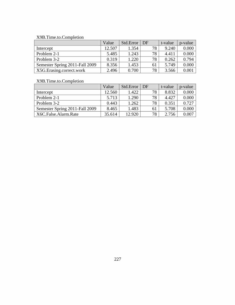
227

X9B.Time.to.Completion

Value Std.Error DF t-value p-value

Intercept 12.507 1.354 78 9.240 0.000

Problem 2-1 5.485 1.243 78 4.411 0.000

Problem 3-2 0.319 1.220 78 0.262 0.794

Semester Spring 2011-Fall 2009 8.356 1.453 61 5.749 0.000

X5G.Erasing.correct.work 2.496 0.700 78 3.566 0.001

X9B.Time.to.Completion

Value Std.Error DF t-value p-value

Intercept 12.560 1.422 78 8.832 0.000

Problem 2-1 5.713 1.290 78 4.427 0.000

Problem 3-2 0.443 1.262 78 0.351 0.727

Semester Spring 2011-Fall 2009 8.465 1.483 61 5.708 0.000

X6C.False.Alarm.Rate 35.614 12.920 78 2.756 0.007

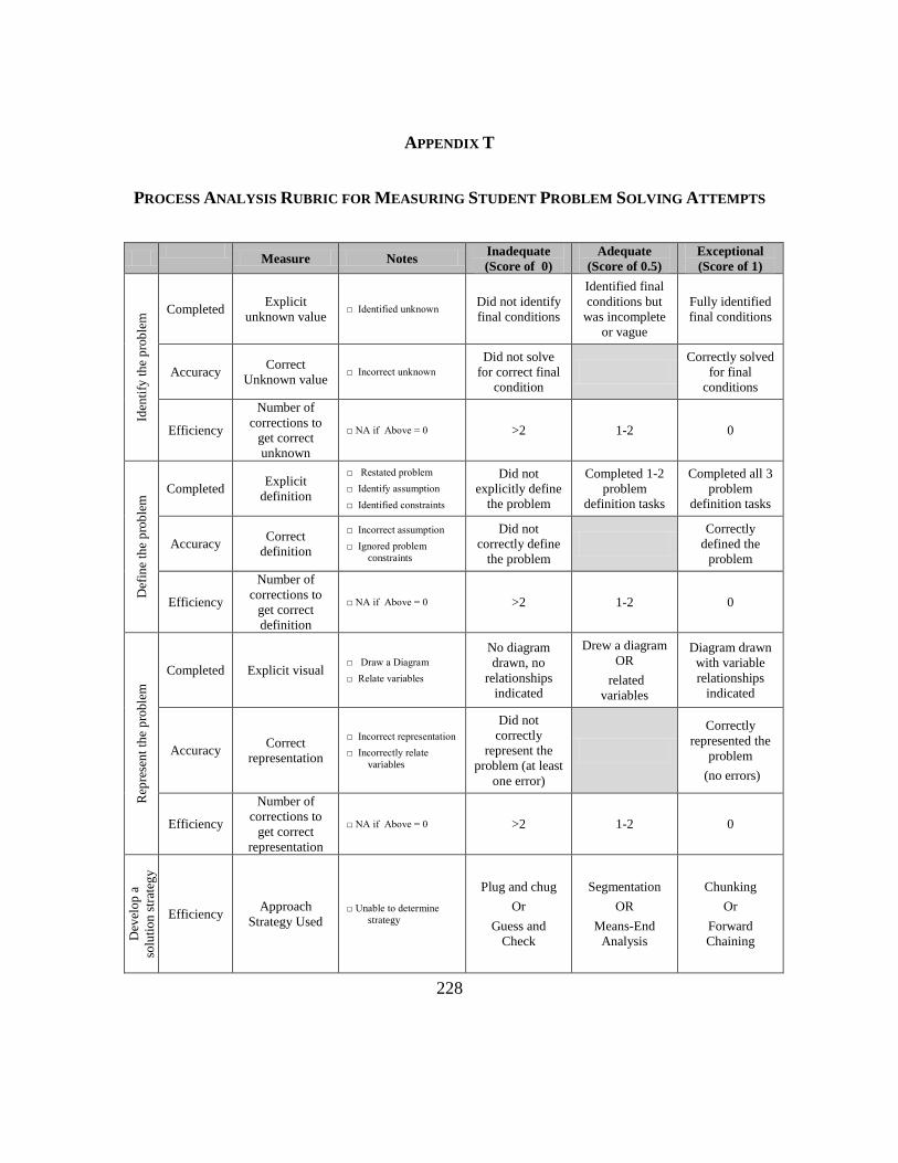
228

APPENDIX T

PROCESS ANALYSIS RUBRIC FOR MEASURING STUDENT PROBLEM SOLVING ATTEMPTS

Measure Notes Inadequate

(Score of 0)

Adequate

(Score of 0.5)

Exceptional

(Score of 1)

Iden

tify

th

e p

rob

lem

Completed Explicit

unknown value □ Identified unknown

Did not identify

final conditions

Identified final

conditions but

was incomplete

or vague

Fully identified

final conditions

Accuracy Correct

Unknown value □ Incorrect unknown

Did not solve

for correct final

condition

Correctly solved

for final

conditions

Efficiency

Number of

corrections to

get correct

unknown

□ NA if Above = 0 >2 1-2 0

Def

ine

the

pro

ble

m Completed

Explicit

definition

□ Restated problem

□ Identify assumption

□ Identified constraints

Did not

explicitly define

the problem

Completed 1-2

problem

definition tasks

Completed all 3

problem

definition tasks

Accuracy Correct

definition

□ Incorrect assumption

□ Ignored problem

constraints

Did not

correctly define

the problem

Correctly

defined the

problem

Efficiency

Number of

corrections to

get correct

definition

□ NA if Above = 0 >2 1-2 0

Rep

rese

nt

the

pro

ble

m

Completed Explicit visual □ Draw a Diagram

□ Relate variables

No diagram

drawn, no

relationships

indicated

Drew a diagram

OR

related

variables

Diagram drawn

with variable

relationships

indicated

Accuracy Correct

representation

□ Incorrect representation

□ Incorrectly relate

variables

Did not

correctly

represent the

problem (at least

one error)

Correctly

represented the

problem

(no errors)

Efficiency

Number of

corrections to

get correct

representation

□ NA if Above = 0 >2 1-2 0

Dev

elo

p a

solu

tio

n s

trat

egy

Efficiency Approach

Strategy Used □ Unable to determine

strategy

Plug and chug

Or

Guess and

Check

Segmentation

OR

Means-End

Analysis

Chunking

Or

Forward

Chaining

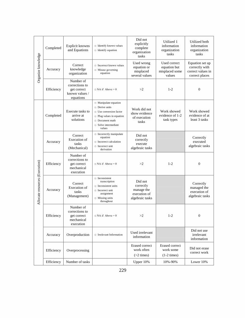
229

Org

aniz

e k

no

wle

dg

e

Completed Explicit knowns

and Equations

□ Identify known values

□ Identify equation

Did not

explicitly

complete

organization

tasks

Utilized 1

information

organization

tasks

Utilized both

information

organization

tasks

Accuracy

Correct

knowledge

organization

□ Incorrect known values

□ Misuse governing

equation

Used wrong

equation or

misplaced

several values

Used correct

equation but

misplaced some

values

Equation set up

correctly with

correct values in

correct places

Efficiency

Number of

corrections to

get correct

known values /

equations

□ NA if Above = 0 >2 1-2 0

All

oca

te r

eso

urc

es (

Ex

ecu

tio

n)

Completed

Execute tasks to

arrive at

solutions

□ Manipulate equation

□ Derive units

□ Use conversion factor

□ Plug values in equation

□ Document math

□ Solve intermediate

values

Work did not

show evidence

of execution

tasks

Work showed

evidence of 1-2

task types

Work showed

evidence of at

least 3 tasks

Accuracy

Correct

Execution of

tasks

(Mechanical)

□ Incorrectly manipulate

equation

□ Incorrect calculation

□ Incorrect unit

derivation

Did not

correctly

execute

algebraic tasks

Correctly

executed

algebraic tasks

Efficiency

Number of

corrections to

get correct

mechanical

execution

□ NA if Above = 0 >2 1-2 0

Accuracy

Correct

Execution of

tasks

(Management)

□ Inconsistent

transcription

□ Inconsistent units

□ Incorrect unit

assignment

□ Missing units

throughout

Did not

correctly

manage the

execution of

algebraic tasks

Correctly

managed the

execution of

algebraic tasks

Efficiency

Number of

corrections to

get correct

mechanical

execution

□ NA if Above = 0 >2 1-2 0

Accuracy Overproduction □ Irrelevant Information Used irrelevant

information

Did not use

irrelevant

information

Efficiency Overprocessing

Erased correct

work often

(>2 times)

Erased correct

work some

(1-2 times)

Did not erase

correct work

Efficiency Number of tasks Upper 10% 10%-90% Lower 10%

230

Mo

nit

ori

ng P

rog

ress

Completed Hit rate <0.25 0.25 < x < 0.5 >.5

Accuracy False alarm rate >0.5 0.2 < x < 0.5 0< x < 0.2

Efficiency Sensitivity (A’) [0.0-0.6) [0.6-0.8) [0.8-1.0]

Ev

alu

ate

the

solu

tion

Completed Check accuracy □ Checked accuracy

□ Indicated final answer

Did not check

accuracy or

indicate final

answer

Checked

accuracy or

indicated final

answer

Checked

accuracy and

indicated final

answer

Accuracy Correct

evaluation

□ Incorrectly manipulate

equation

□ Incorrect calculation

□ Incorrect unit

derivation

Checked

accuracy but

was flawed

Checked

accuracy but

was incomplete

Properly

checked

accuracy

Process Analysis Rubric for Measuring Student Problem Solving Attempts

Performance

Measures Notes

Inadequate

(Score of 0)

Adequate

(Score of 0.5)

Exceptional

(Score of 1)

Solu

tion A

ccura

cy

Answer

Accuracy

Incorrect

Answer or

Gave Up

Correct Answer

but Missing /

Incorrect Units

Correct

Answer

Conceptual

Errors

□ Incorrect assumptions

□ Incorrect representation

□ Incorrectly relate variables

□ Misuse governing equation

Left more

than 1 error

remaining in

the solution

Left 1 error

remaining in the

solution

Left 0 errors

remaining in

the solution

Mechanical

Errors

□ Incorrectly manipulate

equation

□ Incorrect calculation

□ Incorrect unit derivation

Left more

than 1 error

remaining in

the solution

Left 1 error

remaining in the

solution

Left 0 errors

remaining in

the solution

Management

Errors

□ Incorrect unknown value

□ Ignored problem constraints

□ Incorrect known value

□ Inconsistent transcription

□ Inconsistent units

□ Incorrect unit assignment

□ Missing Units Throughout

□ Irrelevant information

Left more

than 2 errors

remaining in

the solution

Left 1-2 errors

remaining in the

solution

Left 0 errors

remaining in

the solution

Pro

cess

Eff

icie

ncy

Error rate

More than

25% 5%<x<25% 0% < x < 5%

Time to

completion Slowest 25% Middle 50% Fastest 25%

231

REFERENCES

Abdi, H. (Ed.) (2009) Encyclopedia of Education (Vols. 3). New York: Elsevier.

Adelman, C. (1998). Women and men of the engineering path: a model for analysis of

undergradute careers. Washington, D.C.: Office of Educational Research and

Improvement.

Albers, M. J. (2005). Communication of Complex Information: User Goals and

Information Needs for Dynamic Web Information: Lawrence Erlbaum Associates

Pub.

Artzt, A. F., & Armour-Thomas, E. (1992). Development of a Cognitive-Metacognitive

Framework for Protocol Analysis of Mathematical Problem Solving in Small

Groups. Cognition and Instruction, 9(2), 137-175.

Baddley, A. (2003). Working memory: Looking back and looking forward. Nature

Review: Neuroscience, 4(10), 829-839.

Barnett, S. M., & Ceci, S. J. (2002). When and where do we apply what we learn?: A

taxonomy for far transfer. Psychological Bulletin, 128(4), 612-637.

Borko, H., Mayfield, V., Marion, S., Flexer, R., & Cumbo, K. (1997). Teachers'

developing ideas and practices about mathematics performance assessment:

Successes, stumbling blocks, and implications for professional development.

Teaching and Teacher Education, 13(3), 259-278.

Bottoms, G., & Anthony, K. (2005). Project Lead the Way: A pre-engineering curriculum

that works. Retrieved from

http://www.sreb.org/programs/hstw/publications/briefs/ProjectLeadTheWay.asp

Bowden, E. M., Jung-Beeman, M., Fleck, J., & Kounios, J. (2005). New approaches to

demystifying insight. TRENDS in Cognitive Sciences, 9(7), 322-328.

Bowman, D., & Benson, L. (2010). MuseInk: Seeing and hearing a freshman engineering

student think. Paper presented at the 2010 ASEE Annual Conference Proceedings.

Brown, J. S., & Duguid, P. (1998). Organizing Knowledge. California Management

Review, 40(3), 90-111.

232

Bruner, J. S. (1973). Going beyond the information given. In J. M. Anglin (Ed.), Beyond

the information given: Studies in the psychology of knowing (pp. 218-238). New

York: Norton.

Chi, M. T., Feltovich, P. J., & Glaser, R. (1981). Categorization and representation of

physics problems by experts and novices. Cognitive Science, 5, 121-152.

Chi, M. T., Glaser, R., & Farr, M. J. (1988). The nature of expertise. Hillsdale, N.J: L.

Erlbaum Associates.

Cohen, G., Kiss, G., & LeVoi, M. (1994). Memory: Current Issues. Buckingham: Open

University Press.

Craig, A. (1979). Nonparametric measures of sensory efficiency for sustained monitoring

tasks. Human Factors, 21(1), 69-78.

Crewell, J. W., Plano Clark, V. L., Gutmann, M. L., & Loomis, D. M. (2003). Advanced

Mixed Methods Research Designs. In A. Tashakkori & C. Teddlie (Eds.),

Handbook of Mixed Methods in Social & Behavioral Research (pp. 229).

Thousand Oaks, CA: Sage Publications, Inc.

Crews, D. (2000). Mathematical Problem Solving Strategies Retrieved September 12,

2009, 2010, from http://www.qerhs.k12.nf.ca/projects/math-problems/intro.html

Damelio, R. (1995). The Basics of Benchmarking: Taylor and Francis.

Drury, C. G. (1990). Designing ergonomics studies and experiments. In J. R. Wilson & E.

N. Corlett (Eds.), Evaluation of human work (2 ed.). London: Taylor and Francis

Ltd.

Elio, R. e., & Scharf, P. B. (1990). Modeling novice-to-expert shifts in problem-solving

strategy and knowledge organization. Cognitive Science, 14(4), 579-639.

Esgate, A., Groome, D., & Baker, K. (2005). An Introduction to Applied Cognitive

psychology. East Sussex: Psychology Press.

Farmer, E., & Brownson, A. (2003). Review of Workload Measurement, Analysis and

Interpretation Methods.

Felder, R. M., Felder, G. N., & Mauney, M. (1995). A longitudinal study of engineering

student performance and retention. III. Gender differences in student

performance and attitudes. Journal of Engineering Education, 84(2), 151-163.

233

FIRST (2010). Retrieved April 9, 2012, from http://www.usfirst.org/

Fuchs, L. S., Fuchs, D., Karns, K., Hamlett, C. L., & Katzaroff, M. (1999). Mathematics

Performance Assessment in the Classroom: Effects on Teacher Planning and

Student Problem Solving. American Educational Research Journal, 36(3), 609-

646.

Funke, J. (1991). Solving Complex Problems: Exploration and Control of Complex

Systems. In R. J. Sternberg & P. A. Frensch (Eds.), Complex Problem Solving.

Hillsdale, New Jersey: Lawrence Erlbaum Associates Inc, .

Gatignon, H. (2009). Statistical Analysis of Management Data (2 ed.): Springer.

Getzels, J. W. (1975). Problem-Finding and the Inventiveness of Solutions. The Journal

of Creative Behavior, 9(1), 12-18.

Getzels, J. W. (1979). Problem Finding: a Theoretical Note. Cognitive Science, 3(2), 167-

172.

Gilbreth, L. (1914). The psychology of management: Sturgis & Walton.

Gravetter, F. J., & Wallnau, L. B. (2008). Statistics for the Behavioral Sciences: Cengage

Learning.

Green, D. M., & Swets, J. A. (1966). Signal detection theory and psychophysics. New

York: John Wiley & Sons.

Greeno, J. G., & Riley, M. S. (1987). Processes and Development of Understanding. In F.

E. Weinert & R. H. Kluwe (Eds.), Metacognition, motivation, and understanding.

Hillsdale, New Jersey: Lawrence Erlbaum Associates Inc.

Grigg, S. J., & Benson, L. C. (2011). Work in Progress: Robust Engineering Problems for

the Study of Problem Solving Strategies. Proceedings of the Frontiers in

Education Conference.

Grigg, S. J., & Benson, L. C. (2012). Effects of student strategies on successful problem

solving. Paper presented at the ASEE Annual Conference.

Gueorguieva R, K. J. H. (2004). Move over anova: Progress in analyzing repeated-

measures data andits reflection in papers published in the archives of general

psychiatry. Archives of General Psychiatry, 61(3), 310-317.

234

Gwet, K. L. (2010). Handbook of inter-rater reliability: The definitive guide to

measuring the extent of agreement upon multiple raters (2 ed.). Gaithersburg,

MD: Advanced Analytics, LLC.

Hambrick, D. Z., & Engle, R. W. (2003). The Role of Working Memory in Problem

Solving. In J. E. Davidson & R. J. Sternberg (Eds.), The Psychology of Problem

Solving. Cambridge, UK: Cambridge University Press.

Harmon, P. (2008). How do you measure processes? Business Process Trends Monthly

Email Advisor, 6(8), 1-2.

Hart, S. G. (2006). NASA-Task Load Index ( NASA-TLX); 20 years later. Paper presented

at the Human Factors and Ergonomics Society Annual Meeting Proceedings.

Hartman, H. J. (2001). Developing students' metacognitive knowledge and skills. In H. J.

Hartman (Ed.), Metacognition in learning and instruction: theory, research and

practice (2 ed., pp. 287). Dordrecht, The Netherlands: Kluwer Academic

Publishers.

Hegarty, M., & Kozhevnikov, M. (1999). Types of visual-spatial representations and

mathematical problem solving. Journal of Educational Psychology, 91(4), 684-

689.

Hutchinson, S. A. (1988). Education and grounded theory. In R. R. Sherman & R. B.

Webb (Eds.), Qualitative research in education: focus and methods. New York,

New York: Falmer Press.

Jablokow, K. W. (2007). Engineers as problem-solving leaders: Embracing the

humanities. IEEE Technology and Society Magazine, 26, 29-35.

Jonassen, D., & Hung, W. (2008). All problems are not Equal: Implications for Problem-

Based Learning. The Interdisciplinary Journal of Problem-Based Learning, 2(2),

6-28.

Jonassen, D., Strobel, J., & Lee, C. B. (2006). Everyday problem solving in engineering:

Lessons for engineering educators. Journal of Engineering Education, 95(2), 139-

151.

Jonassen, D. H. (2004). Learning to Solve Problems. San Fransisco, CA: Pfeiffer.

Jonassen, D. H. (2010). Research Issues in Problem Solving. Paper presented at the 11th

International Conference on Education Research.

235

Kirton, M. J. (2003). Adaption-Innovation in the context of diversity and change. Hove,

Sussex: Routledge.

Konz, S., & Johnson, S. (2004). Operations Analysis Work Design. Scottsdale, Arizona:

Holcomb Hathaway.

Larkin, J., McDermott, J., Simon, D. P., & Simon, H. A. (1980a). Expert and novice

performance in solving physics problems. Science, 208, 1335-1342.

Larkin, J., McDermott, J., Simon, D. P., & Simon, H. A. (1980b). Models of competence

in solving physics problems. Cognitive Science, 4, 317-345.

Lester Jr., F. K. (1994). Musings about mathematical problem-solving research 1970 -

1994. Journal of Research in Mathematics Education, 25(6), 660-675.

Litzinger, T. A., Van Meter, P., Firetto, C. M., Passmore, L. J., Masters, C. B., Turns, S.

R., et al. (2010). A Cognitive Study of Problem Solving in Statics. Journal of

Engineering Education, 99(4), 337-353.

MacGregor, J. N., Ormerod, T. C., & Chronicle, E. P. (2001). Information Processing and

Insight: A Process Model of Performance on the Nine-Dot and Related Problems.

Journal of Experimental Psychology: Learning, Memory, and Cognition, 27(1),

176-201.

Macmillan, N. A., & Creelman, C. D. (2005). Detection theory: a user's guide: Lawrence

Erlbaum Associates.

Malloy, C. E., & Jones, M. G. (1998). An Investigation of African American Students'

Mathematical Problem Solving. Journal for Research in Mathematics Education,

29(2), 143-163.

Marzano, R. J., & Heflebower, T. (2011). Grades that show what students know.

Educational Leadership, 69(3), 34-39.

Matlin, M. W. (Ed.). (2001). Cognition (5 ed.): John Wiley & Sons.

Mayer, R. E. (2008). Information Processing. In T. L. Good (Ed.), 21st century

education: a reference handbook (Vol. 2, pp. 168-171). Thousand Oaks,

California: Sage.

Megaw, T. (2005). The definition and measurement of mental workload. In J. R. Wilson

& N. Corlett (Eds.), Evaluation of Human Work (Vol. 3, pp. 541-542). Boca

Raton, Fl: Taylor & Francis Group.

236

Miller, G. A. (1956). The magical number seven, plus or minus two: Some limits on our

capacity for processing information. The Psychological Review, 63(2), 17.

NASA. from http://humansystems.arc.nasa.gov/groups/TLX/downloads/TLXScale.pdf

Nation, D., & Siderman, S. (2004). Mathematics Problem Solving Coach, Strategies and

Applications (Vol. 1). New York: Triumph Learning.

National Academy of Engineering (2004). The Engineer of 2020: Visions of Engineering

in the New Century. Washington, D.C.: National Academies Press.

National Research Council . Retention Task Force, & National Research Council .

Committee on Minorities in Engineering (1977). Retention of minority students in

engineering: a report of the Retention Task Force: National Academy of

Sciences.

Nickerson, R. S. (1994). The teaching and thinking of problem solving. In R. J. Sternberg

(Ed.), Thinking and Problem Solving (2 ed., pp. 409-449). San Diego: Academic

Press.

Nilson, L. B. (2003). Teaching at its Best (2 ed.). San Francisco, CA: Jossey-Bass.

Novak, J. D., & Gowin, D. B. (1984). Learning how to learn. Cambridge, United

Kingdom: Cambridge University Press.

O'Connor, K. (2010). A Repair Kit for Grading: Fifteen Fixes for Broken Grades:

ADDISON WESLEY (PEAR.

Ohland, M. W., Sheppard, S. D., Lichenstein, G., Eris, O., & Charchra, D. (2008).

Persistence, engagement, and migration in engineering programs. Journal of

Engineering Education, 97(3), 259-278.

Owhoso, V. E., Messier, W. F., & Lynch Jr., J. G. (2002). Error detection by industry-

specialized teams during sequential audit review. Journal of Accounting

Research, 40(3), 883-900.

Parasuraman, R., Masalonis, A. J., & Hancock, P. A. (2000). Fuzzy signal detection

theory: basic postulates and formulas for analyzing human and machine

performance. Human Factors, 42(4), 636-659.

Perry, W., Broers, A., El-Baz, F., Harris, W., Healy, B., Hillis, W., et al. (2008). Grand

Challenges for Engineering. Washington, DC.

237

Peterson, P. L., Fennema, E., Carpenter, T. P., & Loef, M. (1989). Teachers' Pedagogical

Content Beliefs in Mathematics. Cognition and Instruction, 6(1), 1-40.

PLTW, S. (2012). What is PLTW?, April 9, 2012, from

http://www.southcarolinapltw.com/About_PLTW.html

Polya, G. (1957). How to solve it. Garden City, New York: Doubleday.

Pretz, J. E., Naples, A. J., & Sternberg, R. J. (2003). Recognizing, Defining, and

Representing Problems. In J. E. Davidson & R. J. Sternberg (Eds.), The

Psychology of Problem Solving. Cambridge, UK: Cambridge University Press.

Proctor, R. W., & Van Zandt, T. (2008). Hyman Factors in Simple and Complex Systems

(2 ed.). Boca Raton, Florida: Taylor and Francis Group.

Radatz, H. (1980). Students' errors in the mathematical learning environment. For the

learning of Mathematics, 1(1), 16-20.

Ramsay, R. J. (1994). Senior/Manager difference in audit workpaper review

performance. Journal of Accounting Research, 32(1), 127-135.

Reeves, D. (2008). Effective Grading. Educational Leadership, 65(5), 85-87.

Reeves, D. B. (2002). Making standards work: how to implement standards-based

assessments in the classroom, school, and district: Advanced Learning Press.

Rosenthal, J. A. (2012). Statistics and Data Interpretation for Social Work: Springer

Publishing Company.

Rugarcia, A., Felder, R. M., Woods, D. R., & Stice, J. E. (2000). The future of

engineering education I. A vision for a new century. Chemical Engineering

Education, 34(1), 16-25.

Russo, R. (2003). Statistics for the Behavioural Sciences: An Introduction: Psychology

Press.

Samsonowa, T. (2011). Industrial Research Performance Management: Key

Performance Indicators in the ICT Industry: Springer.

Scheer, A. W. (2003). Business process change management: ARIS in practice: Springer.

Seltman, H. J. (2012). Experimental Design and Analysis Available from

http://www.stat.cmu.edu/~hseltman/309/Book/Book.pdf

238

Sheskin, S. A. (2004). Handbook of parametric and nonparametric statistical procedures

(3 ed.). Boca Raton: Chapman & Hall.

Simon, D. P., & Simon, H. A. (1978). Individual differences in solving physics problems.

In R. S. Sigler (Ed.), Children's Thinking: What Develops? NJ: Lawrence

Erlbaum.

Slater, T. F. (1993). Performance Assessment: Adapted from Laboratory performance

assessment. The Physics Teacher, 31(5), 306-309.

Smith, G. F. (1998). Quality problem solving: ASQ Quality Press.

Stahovich, T. (2012). Using digital pens to automatically predict student performances in

engineering statics. Paper presented at the 2012 National Science Foundation

Engineering Education Awardees Conference Washington, D.C.

Stammers, R. B., & Shepherd, A. (1990). Task Analysis. In J. R. Wilson & E. N. Corlett

(Eds.), Evaluation of Human Work (2 ed., pp. 145-168). Great Britain: Taylor &

Francis Ltd.

Stanton, N., A., Salmon, P. M., Walker, G. H., Baber, C., & Jenkins, D. P. (2005).

Human Factors Methods: A practical guide for engineering and design.

Burlington, VT: Ashgate.

Stephan, E. A., Park, W. J., Sill, B. L., Bowman, D. R., & Ohland, M. W. (2010).

Thinking Like an Engineer: An Active Learning Approach: Pearson Education.

Sternberg, R. J. (1985). Beyond IQ: A Triarchic Theory of Human Intelligence. New

York: Cambridge University Press.

Sweller, J. (1988). Cognitive load during problem solving: effects on learning. Cognitive

Science, 12, 257-285.

Szetela, W. (1987). The problem of evaluation in problem solving: Can we find

solutions? Arithmetic Teacher, 35(3), 36-41.

Tashakkori, A., & Teddlie, C. (1998). Mixed Methodology (Vol. 46). Thousand Oaks,

CA: Sage Publications.

Taylor, F. W. (1911). The principles of scientific management: Harper & Brothers.

239

Varnad, T. E. (2005). The effects of a technological problem solving activity on FIRST

LEGO League Participants' problem solving style and performance. Virginia

Polytechnic Institute and State University, Blacksburg, Virginia.

Wallas, G. (1926). The art of thought. London: J. Cape.

Wang, Y., & Chiew, V. (2010). On the cognitive process of human problem solving.

Cognitive Systems Research, 11(1), 81-92.

Wankat, P. C. (1999). Reflective analysis of student learning in a sophomore engineering

course. Journal of Engineering Education, 88(2), 195-203.

Warm, J. S., Matthews, G., & Finomore Jr., V. S. (2008). Vigilance, Workload, and

Stress. In P. A. Hancock & S. J. L. (Eds.), Performance Under Stress (pp. 115-

141). Burlington, VT: Ashgate Publishing Company.

Weston, C., Gandell, T., Beauchamp, J., McAlpine, L., Wiseman, C., & Beauchamp, C.

(2001). Analyzing interview data: The development and evolution of a coding

system. Qualitative Sociology, 24(3), 381-400.

Wickens, C. D. (1984). Engineering psychology and human performance. Columbus,

Ohio: Merrill.

Wickens, C. D., Gordon, S. E., & Liu, Y. (1998). An introduction to human factors

engineering: Longman.

Wilson, J. R., & Corlett, E. N. (2005). Evaluation of human work (3 ed.). Boca Raton,

Florida: CRC Press.

Wilson, J. W., Fernandez, M. L., & Hadaway, N. (1993). Mathematical Problem Solving.

In P. S. Wilson (Ed.), Research Ideas for the Classroom: High School

Mathematics. New York: MacMillan.

Wong, R. M. F., Lawson, M. J., & Keeves, J. (2002). The effects of self-explanation

training on students' problem solving in high-school mathematics. Learning and

Instruction, 12(1), 233-262.

Woods, D. R., Felder, R. M., Rugarcia, A., & Stice, J. E. (2000). The future of

engineering education III. Developing critical skills. Chemical Engineering

Education, 34(2), 108-117.

Zhu, Z. (2007). Gender differences in mathematical problem solving patterns: A review

of literature. International Education Journal, 8(2), 187-203.