Utah State University Utah State University

DigitalCommons@USU DigitalCommons@USU

Reports Utah Water Research Laboratory

January 1973

A Preliminary Model of the Hydrologic-Sociologic Flow System of A Preliminary Model of the Hydrologic-Sociologic Flow System of

an Urban Area an Urban Area

Wade H. Andrews

J. Paul Riley

Craig W. Colton

George B. Shih

Malcolm B. Masteller

Follow this and additional works at: https://digitalcommons.usu.edu/water_rep

Part of the Civil and Environmental Engineering Commons, and the Water Resource Management

Commons

Recommended Citation Recommended Citation Andrews, Wade H.; Riley, J. Paul; Colton, Craig W.; Shih, George B.; and Masteller, Malcolm B., "A Preliminary Model of the Hydrologic-Sociologic Flow System of an Urban Area" (1973). Reports. Paper 641. https://digitalcommons.usu.edu/water_rep/641

This Report is brought to you for free and open access by the Utah Water Research Laboratory at DigitalCommons@USU. It has been accepted for inclusion in Reports by an authorized administrator of DigitalCommons@USU. For more information, please contact digitalcommons@usu.edu.

A PRELIMINARY MODEL OF THE HYDROLOGIC-SOCIOLOGIC

FLOW SYSTEM OF AN URBAN AREA

Prepared by

Wade H. Andrews J. Paul Riley

Craig W. Colton George B. Shih

Malcolm B. Masteller

The Institute for Social Science Research on Natural Resources

and Utah Water Research Laboratory

This study is funded by the Office of Water Resources Research

United States Department of the Interior Title II Project Number 14-31-000 1-3712

Utah Water Research Laboratory College of Engineering Utah State University Logan, Utah 84322

April 1973 PRWGI09-1

TABLE OF CONTENTS

Chapter I ..... .

INTRODUCTION

Organization of the Report Problems and Objectives . Elements of Flood Management The Study Area . . . . . . . Specific Objectives ..... The Process of Model Development Conceptualizing the Hydrologic-Sociologic System

Chapter II

MODEliNG THE HYDROLOGIC COMPONENT OF THE SYSTEM

The Conceptual Model of the Urban Hydrologic System The Hydrologic Balance ....... . Time and Space Increments . . . . . . . The Hydrologic Characteristics of the Study

Location . Topography Climate Geology Drainage conditions Instrumentation . .

The Degree of Urbanization within the Study Area

Computation of urban parameters Summary of calculated urban parameters

Precipitation and Streamflow Inputs to the Hydrology Model Model Verification ...... . Streamflow Predictions by the Model

Chapter III ............. .

SOME MATHEMATICAL TECHNIQUES FOR MODELING SOCIOLOGIC RELATIONSHIPS

Introduction . Methodological Approach Study Area ..... . Data Collection and Identification of Social Variables

SUlVey data . . . . . Agency and group data

v

Page

1 1 2 2 3 3 5

7

7

7 7

10 11

11 11 11 11 11 14

14

16 20

20 20 24

29

29

29 29 29 29

29 30

TABLE OF CONTENTS (Continued)

Statistical Techniques Applied to Social Data

Page 30

The multiple regression technique Standardization of measurements Statistical assumptions ., . . . Social applications of regression analysis

30 32 32 33

An Example of the Development of a Sociologic Regression Relationship . . . . . . . . . . . . . 33

Description of the independent variables The general equation . . . . . . Stratification of sociologic sampling

34 35 35

CHA.P'fER IV . . . . . . . . . . . . . . . . . . . . . . . . . . . . . . . . . . 37

IDENTIFYING THE COMPONENTS OF THE SOCIOLOGIC ACTION PROCESS SUBSYSTEM ........................... 37

A Conceptual Model of the Hydrologic-Sociologic Flow System . . . . . . . 37 Section One: Public Opinion ...... 37

Public perception of flood probabilities 39 Concern about flooding . . . . . . 39 Flooding experienced during lifetime 40 Other secondary variables 40 ~mm~ . . . . . . . . ~

Section Two: Planning AgenCies 40

Characteristics of planning agencies 40

Identifying and Evaluating Planning Problems 42

Non-emergency solution evaluation 45 Acceptance functions ..... 46 Minimum acceptance level 47 Application of adjustment perception 49 Secondary variables in Section Two of the conceptual model 49 Variables identified and defined 49 Mathematical relationships ........ 51 Five methods of flood control . . . . . . . 51 Emergency solution recognition and evaluation 53

Section Three: The Decision Agencies 54 Section Four: Public Reaction 55

Population attitude toward proposed flood control actions . . . . . . . . . . . . . . . . . . 56 Overt opposition to flood control by members of population ................ 56 Other factors related to opposition to flood control 58

Section Five: Alternative Actions 59 Section Six: Implementation of Action Plan 59

Chapter V 61

vi

TABLE OF CONTENTS (Continued) Page

SUMMARY OF THE MODEL AND RECOMMENDATIONS 61

Steps in Model Development 61 The Hydrologic Dimension 61 The Sociologic Dimension 62

Section one, public opinion 62 Section two, planning agencies 62 Section three, the decision agencies 67 Section four, public reaction to decisions 67 Section five, alternative action 67 Section six, implementation 67

In Summary 67 Recommendations 68

BIBLIOGRAPHY 69

APPENDICES . 75

Appendix A - Computer Program-Hydrologic System 77 Appendix B - Social Variables Used in the Model* 83 Appendix C - Selected Questions from Interview Schedule on

A Study of Public Opinions Related to Flooding in the Salt Lake Valley . . . . . . . . . . . . . . . . . . . . . . 85

vii

LIST OF FIGURES

Figure

1.1 Salt Lake County

1.2 Steps in the development of a model of a real world system

1.3

2.1

Preliminary concepts and interactions relating to the sociologic part of the hydrologic-sociology system and their relationship to the hydrologic part of the model . . . . . . . . .

Schematic representation of the steps used to obtain the runoff hydrograph ............... .

2.2 Schematic diagram to obtain surface outflow. The dotted line indicates the processes considered in this study

2.3 Schematic diagram of an urban subwatershed model

2.4 The urbanized study area

Page

3

4

6

8

9

10

12

2.5 Topography from the Wasatch Mountains to the Jordan River 13

2.6 Dividing the watersheds into subzones . . . . . . . . . 14

2.7 Hydrologic instrumentation and the Thieissien polygons for precipita tion analysis within the study area ..... ........... 15

2.8 Typical urban residential block showing the pervious and the impervious areas .............. 17

2.9 A sample of dividing subzones into smaller spatial units 18

2.10 Sketch illustrating the characteristic impervious length, 4, for a given watershed or subzone ...... 19

2.11 Isohyetallines for the event of May 22-23, 1968 22

2.12 Recorded precipitation and streamflows and agreement achieved between computed and observed outflows for the event of May 23, 1968 ..... 23

2.13 Peak discharge vs. return frequency at different stages of urbanization (Cf ) ............................ 25

2.14 Peak discharge vs. return frequency at different stages of urbanization (Cf ) ........•................... 26

2.15 Peak discharge vs. return frequency at different stages of urbanization (Cf ) ................ . . • . . 27

4.1 Flow chart of the conceptual model of the sociologic-hydrologic system ....................... . ..... 38

viii

Figure

4.2

4.3

5.1

LIST OF FIGURES (Continued)

Page Identified important steps or components of the agency decision process ............... . 43

Diagram of evalua tion process by agency or other group 48

Mathematical model of the sociological dimension of the hydrologic-sociologic flow system ........ . . . . . . . . . . . . . 64

LIST OF TABLES

Table Page

2.1 Characteristics of the main drainage channels of Mill, Big Cottonwood, and Little Cottonwood Creeks within the study area . . . . " ...... 14

2.2 Physical characteristics for the Mill Creek, Big Cottonwood Creek, and Little Cottonwood Creek drainages .......... ........ 21

2.3 Precipitation and discharge ranges for various storm frequencies at the gages indicated . . . . . . . . . . . . . . . . . . . . . . . . 24

3.1 Variables found important in one or more regression equations and their theoretical ranges as presently measured .....

4.1 Explanation of decision blocks shown by Figure 4.2

4.2 Significant variables for attitudes toward flood actions

4.3 Relationship between attitude and overt opposition to flood control by channelization and lining of streams for two zones within the study area ..... .

5.1 Variables used in Figure 5.1

ix

31

44

50

57

65

CHAPTER I

INTRODUCTION

This report describes the first phase of a larger study which is directed toward the development of a gerieral technique for analyzing and solving urban metropolitan hydrologic problems through a joint con­sideration of both the physical and social dimensions. This report is limited to the preliminary work of identification of social variables, the first steps in assigning mathematical values to them, and developing a mathematical format for these variables. In addition, the physical-hydrologic system is identified for purposes of clarifying the elements in that system. The ultimate objective of the entire study is directed toward discover­ing a theoretical and generally applicable mathematical model of both the physical and social dimensions involved in metropolitan flooding problems.

Conceptualizing the real world system, or proto­type, and identifying the most probable causal elements are among the first steps of any undertaking of this nature. In this first phase many variables and relationships were examined and an effort was made to identify components which may eventually be linked together to form a realistic model of the total system. Thus, the main goal of the work reported here was to lay the ground work for a model by defining elements of a system to be modeled and to formulate basic modeling concepts. In subsequent phases of the study, efforts will be made to integrate the various model components, and calibrate, test, and improve the model through the use of other data collected for a specific site. It is envisioned that the study, when completed, may form the baSIC framework of a comprehensive technique which will provide planners and managers with a method of estimating possible hehavior for both physical and social consequences of action alternatives relating to the solution of urban flooding problems.

Organization of the Report

The report is divided into five parts. Chapter I introduces the problem and sets out the scope of the study. Chapter II is concerned with the development of the hydrologic dimension of the model. The hydrologic model for the study of the area is discussed by this chapter. The methodology and rationale used in develop­ing the conceptual model of the sociological component of the system are presented by Chapter III. A conceptual model of the hydrologic-sociologic system, together with generalized mathematical relationships for specific socio­logical processes, are included in Chapter IV. Finally, the summary and conclusions for the first phase of the overall study are set out in Chapter V. Specific data, computer programs, and other relevant information are included as appendices.

Pro blerns and Objectives

Current procedures applied to the control of urban flooding problems do not adequately consider all of the needs of complex modern society. Decisions involving the development and management of water resources should be based on sound social as well as technological and economic considerations. In a public process under a democratic form of government it is assumed that this decision procedure may include public involvement. This concept of involvement recognizes that the physical system may be adjusted to achieve particular social goals or objectives.

The two major dimensions of the problem examined in this project are the physical or hydrologic factors and the social aspects related to water control. Because perturbations or modifications in terms of either dimen­sion cause changes throughout the entire system, both of these interrelated dimensions are basic to final action which is aimed at reaching desired goals. Urban develop­ment changes not only the physical characteristics of the land, but also introduces complex social ramifications. High population densities, for example, magnify the severity of flooding which, in turn, produces ecological problems, as well as endangering human life and property. However, it may be possible to develop a flood manage­ment program within a particular metropolitan area so as to provide, in addition to flood amelioration, other advantages such as recreational opportunities, aesthetic benefits, enhanced land values, increased water supplies, a modified micro-climate, and a carrier for municipal wastes. By evolving suitable procedures it should be possible to effect many improvements in metropolitan flood drainage systems that simultaneously provide other important direct benefits to a broad sector of the society.

The physical and economic aspects of a drainage problem are usually fairly well understood, while the social aspects are traditionally accorded little consider­ation. The importance of the latter dimensions, however, is becoming increasingly recognized. W. R. D. Sewell (1969, pg. 3) noted:

Social guides comprise a wide variety of influences that encourage or discourage development taking place in particular ways. They include informal influences such as social mores, customs, and atti­tudes, and formal influences such as laws, policies, and administrative arrangements. Knowledge of the effects of such factors is essential to sound water resources planning.

In order to incorporate the effects or influences noted by the above citation into an objective planning model, it is necessary to identify them specifically and place them in a

set of value scales which can be treated in quantified form.

Specifically. the objectives of this phase of the project are as follows:

1. To define the problem involving flood control metho ds in urban areas.

2. To define and identify both the hydrologic and the sociologic components of the total system, including linkage processes between these two components.

3. To evaluate available data, define needs for additional data, and establish data collection procedures.

4. To develop basic concepts for a model of the hydrologic-sociologic system.

Elements of Flood Management

Flood management in urban areas is complex for a number of social and physical reasons:

1. Natural runoff patterns are greatly modified by urban development. The problem, then, is one of predicting urban developments and of assessing their effects upon the runoff process.

2. Piecemeal solutions to urban drainage prob­lems often result from limited capital, local­ized interest, and other causes.

3. Identification of beneficiaries and accurate allocation of costs and benefits is usually difficult in densely settled urban areas.

4. Conflicts of interest often result in delay, compromise, or abandonment of well­intentioned development plans. Such conflicts may be the result of intensive interest or too little interest from the parties involved or may result from lack of understanding of others' pro blems or viewpoints. This problem is fur­ther complicated by the fact that political subdivisions often do not coincide with natural drainage areas.

5. Conflicting attitudes of people produce diffi­culties. People are often suspicious of the motives of public officials. Land owners may strongly resist giving up present advantages for increased flood control or other benefits; an example would be property along stream banks which may be needed for flood control through such methods as channelization or streamside park development. Further, people often are unwilling to contribute to the solution of a problem which does not directly affect them.

The problem of flood management in urban areas is, therefore, taking into account the various technological, economic, and social aspects involved, balancing these elements in a management scheme. The very dynamic nature of the total physical and social system further

2

compounds the difficulties. The problem is complex, but its solutions can be vital to the continued progress and development of urban areas~

The model of the hydrologic-sociologic system toward which this first phase of study is directed will include much of the complexity of this system and will provide a means of evaluating various possible flood control alternatives such as detention dams, lined chan­nels, natural channels, storm sewers, and other control measures that might be available in a given situation.

The Study Area

A specific study site was selected in order to provide a basis for developing a conceptual model and for subsequent model development and testing. This area is a part of the rapidly developing metropolitan area of Salt Lake County which includes Salt Lake City and several other suburban communities. Because of rapid urban growth within this region, the problem of flood drainage and its amelioration is of increasing concern to city and county officials.

The Salt Lake Valley, which is part of the Great Basin, is "U" shaped, bordered on three sides by mountains and by the Great Salt Lake on the north. The valley, which is about 15 tpiles wide (east and west) and 25 miles long, is bisected by the Jordan River which flows northward and discharges into the Great Salt Lake. The average elevation of the valley floor is approximately 4,000 feet above mean sea level. In a hydrologic sense, the Wasatch Mountain Range which borders the eastern side of the valley is especially important because these mountains provide a large portion of the water supplies for the valley below. Several small streams run westward from mountain canyons into the valley and discharge into the Jordan River. The Wasatch Mountains, with peaks up to 11,000 feet above sea level, rise abruptly to a height of nearly 6,500 feet above the valley floor. Because of this height, much of the precipitation which falls on water­sheds within the range is produced by the orographic lifting of air masses which are moving in an easterly direction. The valley floor is considered to be semi-arid with an average of about 15 inches of rainfall per year.

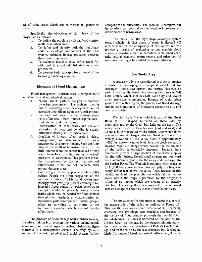
The site selected for this study is limited to a part of the eastern side of the valley as outlined by Figure 1.1. This specific area was chosen because of its urbanizing character, the hydrologic data available, and because of the history of flood control proposals that would affect the inhabitants. This area is bordered on the west by the Jordan River, on the east by the Wasatch Mountains, on the north by the heavily urbanized Parley's Creek drain­age, and on the south by the less urbanized but developing little Cottonwood Creek watershed. Altogether, the area

" • . I.. ~ · . f · . I · •

. .

t-~ :~ .. .",."., \. . • \.,.. ..

Figure 1.1 . Salt Lake County.

contains about half of the eastern section of the Salt Lake Valley.

The popUlation within the study site, according to the 1970 census, is 131 ,882. It is of varying density and growing rapidly. From the current figure of 383,035 people, the Salt Lake Valley popUlation is expected to grow to about 785,000 people by 1985. The study site's contingency to the central business district of Salt Lake City and also its present rate of development suggest that a large part of this expected growth will occur in the study area. This conclusion is supported by the master plan for the county (A Master Plan for Salt Lake County, 1965). The area has a long history of flooding (Corps of Engin.eers, 1969-A, p. 11-19), but continuing urban developments are producing an increasing urgency in the nature of the flood problems. Some of the present development is occurring in the flood plains and canyons, and "new residential developments are rapidly expanding ... " (Corps of Engineers, 1969-A, p. 5). This urban growth not only alters runoff relationships by producing higher peak flows, but also increases the damage potential from a flood of a particular magnitude.

N

t .~··~··.r-·i .. ~. \

•

> . . ~ .. \ . .

~ \

.".."./ .. •

", .. ",., r··""'-

. .

/ .. /' .. ..

3

Specific Objectives

The specific objectives for the first phase were: 1. Identification and specification of the socio­

logic and hydrologic components of the system.

2. Development of conceptual models of the sociologic and hydrologic subsystems, and the formulation of appropriate mathematical ex­pressions for describing the processes of the conceptual model.

3. Test, to a limited degree, the validity of various mathematical representations pro­posed for the model structure, particularly those for linking of the hydrologic and social subsystems.

The Process of Model Development

A model is an abstraction from reality, and in this sense is a simplification of the real world which forms the basis of the model. The degree of simplification is a function of both intent or planning and knowledge about

the real world. Forrester (I961) pointed out that verbal information and conceptualization may be translated into mathematical form for eventual use in a computer. Therefore, the model development process should proceed from the verbal symbols which exist in both theoretical and empirical studies to the mathematical symbols which will comprise the model. '

The development of a working mathematical model requires two major steps. The first step is the creation of a conceptual model which represents to some degree the various elements and systems existing in the real world. This conceptualization is based on known information and hypotheses concerning the various elements of the system and their interrelationships. These conceptuali­zations and hypotheses of the real world of the study area must, of course, be formulated in terms of the available data. Efforts were made to use the most pertinent and accurate data available in creating the conceptual model. As additional information is obtained, the conceptual model will be improved and revised to more closely approximate reality.

The second major step in the development of a working mathematical model is between the conceptual model and the mathematical model itself. The mathe­matical model is the one that is programmed into a computer to simulate the system. During this step an

Real 1-1 Q)

.f,.J

World .-l .r-! ~

Step 1

If

attempt is made to express in both mathematical and verbal forms the various processes and relationships identified by the conceptual model. Thus, the strategy involves a conversion of concepts concerning the real world into terms which can be programmed on a computer. This step usually requires further simplifi­cation, and the resulting working model may be a rather gross representation of real life.

The loss of information, first between the real world and the conceptual model, and second between the conceptual model and computer implementation may be likened to filtering processes as shown by Figure 1.2. The real world is "viewed" through various kinds of data which are gathered about the system. These additional data usually produce an improved conceptual model in terms of time and space resolutions. The improved conceptual model then provides a basis for improvements in the working model. Output from the working model can and will, of course, be compared with corresponding output functions from the real world; when discrepancies exist between the two, adjustments are indicated in both the conceptual. model and the working model.

In this study various physical and social processes as well as system relationships have been conceptualized, and from these conceptualizations significant variables have been identified for use in the model. Equations for

~ (J) .f,.J .-l 'r-! Working ~

Model/Z

/ /

tt /

Figure 1.2. Steps in the development of a model of a real world system.

4

describing some of the relationships in the conceptual model have been developed and tested in a preliminary way for both the physical and social components of the total system.

As the study continues, more data will be gathered and the conceptual model will be improved. Relationships will be more clearly described and further specification will be made for some of the system variables and their relationships. Changes in the working model will be suggested by improvements in the conceptual model, and consequently discrepancies between the output from this model and the real world will be reduced.

Conceptualizing the Hydrologic-Sociologic System

In the first attempt at conceptualization the socio­logical part of the hydrologic-sociologic flow system was envisioned as being composed of interrelated and inter­acting subsystems or parts.

The most general and fundamental property of a system is the interdependence of parts or variables. Interdependence consists of the existence of deter­minate relationships among the parts or variables as contrasted with randomness of variability ... (Par­sons and Shils, 1951, p. 107)

The parts having this interdependence in a system can be called the elements of the system. Systems are seen as being composed of interrelated, connected, and inter­acting components or elements which are linked together so as to form a unity or whole. A subsystem is a part of the larger system which can be integrated into the larger system being referred to. The analysis of a system consists largely in identifying the system elements and determining the characteristics of the interrelationships between them.

Social systems, those which are composed largely of social elements, vary greatly in size, with some having many interrelated and interacting elements and others having only a few. Behavioral research and theory indicate that there are cultural commonalities of characteristics, values, and behavior which exist among individuals. These commonalities provide the basis for the formation of the social subsystems.

Figure 1.3 illustrates several of the interacting classes of components which are regarded as being a part of the conceptual model of the social system as a whole.

5

These components include:

1 . Individuals

2. Governing or regulating institutions or bodies at all levels (federal, state, or local) including executive, legislative and judicial functions.

3. Other institutions (for example, educational, economic, and religious).

4. Other groups (for example, special interest groups, etc.).

Individuals outside of groups are included in the conceptual model of this study because they are seen as being able to influence watershed management policies not only in the capacity of owner or manager but also through their interaction with social subsystems. Of course, it is recognized that the social subsystems are composed of individuals, and individuals within a sub­system are seen as acting as part of that subsystem. The total conceptual model is able to include an individual acting both as a single unit and as a part of a group of individuals acting ~ogether as an element within other subsystems.

One individual can interact within or in relation to more than one subsystem. In this manner some individuals have greater influence or play a greater role in the formation and implementation of resource policy than others. Also, the amount of "input" that can be intro­duced into a particular subsystem by an individual varies from person to person and from system to system.

The direct implementation of a management decision is the output or response function of a social system. This output is viewed as coming from either government (public) management or from private manage­ment (Figure 1.3). As with a physical system for a particular set of output functions, responses of social systems vary both spatially (from system to system) and temporally. For example, individuals and groups possess specific attitudes in relation to many factors such as aesthetics and recreation. These attitudes differ between individuals or groups and also change with time.

Implementation of management decisions can be represented in the hydrologic-sociologic model as social impacts upon the physical component of the system. These impacts produce certain changes in the physical characteristics or parameters of the watershed as represen­ted in the hydrologic part of the model (Figure 1.3). The hydrologic component of the model includes the physical and biological conditions of the watershed. Thus, socially

induced changes in the watershed are reflected in the response functions of the hydrologic system, and this change is fed back as an input to the social system in the mathematical-physical model. This will be done in equa­tions by terms which represent values of important effects of the respective systems upon each other. In this way physical changes, in turn, influence the social system, and so through a set of interactive linkages between the two subsystems a dynamic interaction process occurs within the system as a whole.

Figure 1.3 displays some of the system concepts that were developed in the early stages of this study. It is recognized that the figure depicts a Simplistic summary of the conceptual model, its component subsystems, and their linkages. Each subsystem within the social com­ponent of the overall model is very broad and includes many related and interacting processes. Further develop­ment of the conceptual model of the social component and some corresponding mathematical relationships are presented in Chapters III and IV.

CATEGORIES OF SOCIAL SYSTEMS

Governing or Regulating Institutions or Bodies at all levels (Federal, State, or Local) including Executive, Legislative, and Judicial functions

Other Institutions Educational Religious Etc.

Other Groups (All types not included elsewhere in the model)

Individuals

---

MANAGEMENT IMPLEMENTATION

U Government (Public)

-- Management Implementation

~---- ---

Uprivate (N on- gove rnment)

~ ~-Management I ~ Implementation

LEGEND =Two way Inter­

section ~Management

Implementa -tion

--E -Response of the Watershed (Hydro­logic Model) to Management

HYDROLOGIC OR PHYSICAL MODEL

Urban Watershed (Hydrologic Model)

Figure 1.3. Preliminary concepts and interactions relating to the sociologic part of the hydrologic-sociology system and their relationship to the hydrologic part of the model.

6

CHAPTER II

MODELING THE HYDROLOGIC COMPONENT OF THE SYSTEM

A primary objective of effective watershed manage­ment is to provide optimum benefits to mankind under a range of land use patterns. For example, it is frequently necessary to manage a municipal watershed so as to integrate many of the requirements of a modern com­munity such as residential housing, business locations, water supply, sewage disposal, and recreation. Land uses in an urban area become drastically different from those of natural conditions. Thus, the watershed manager is faced with the need to predict ·system responses under various possible use alternatives. One approach to this problem is to apply the technique of computer simula­tion, whereby a quantitative mathematical model is developed for investigating and predicting the behavior of the system. In the study reported here, a computer model is used to simulate the hydrologic responses of an urban watershed, emphasizing the measurable variables related to the effects of urbanization. The model represents the interrelated processes of the system by functions which describe the different components of physical phenomena on the watershed. Thus, the model is a useful tool for the creative manipulation of the system, and it also facilitates appraisals of proposed changes within the corresponding prototype.

The Conceptual Model of the Urban Hydrologic System

The hydrologic model utilized in this study is a modified version of that developed in earlier studies involving the computer simulation of urban watersheds (Narayana et aI., 1969, and Evelyn et aI., 1970). The basis of the hydrologic model is a fundamental and logical mathematical representation of the various hydrologic processes and routing functions. These physical processes are not specific to any particular geography, but rather are applicable to any hydrologic unit, including the subbasins located within the Salt Lake County study area.

The outflow hydrograph is computed in the model by chronologically deducting from precipitation and streamflow input functions losses due to interception, infiltration, and depression storage and then routing the

7

remainder through surface and channel storages (Figure 2.1). Testing and verification of the basic mathematical model is done by using observed rainfall and runoff data from instrumented runoff areas. In the verification pro­cess coefficients representing interception, depression storage, and infiltration are determined by the trial and error process on the computer such that the outflow hydrograph predicted by the model is nearly identical to the corresponding measured hydrograph from the proto­type. Relationships between these coefficients and various urbanization characteristics or parameters, such as percent impervious cover, are established. These relationships can be applied in predicting the effects of future urban development. A schematic flow diagram of a typical hydrologic system is shown by Figure 2.2. Because of the short time increment involved in urban runoff events, it usually is necessary to be concerned only with the surface runoff component of the system. For this reason, pro­cesses concerned with groundwater storage and movement and evapotranspiration are not included in the hydrologic model of this study. Those transfer processes and storage locations included within the model are shown within the dotted line of Figure 2.2.

In addition to data, experimental and analytical results are used whenever possible to assist in establishing and testing the mathematical relationships included with the model. Average values of hydrologic quantities needed for operation of the hydrologic model are estimated in one of three ways: (1) From available data; (2) by statistical correlation techniques; and (3) through calibra­tion of the model itself.

The Hydrologic Balance

A dynamic system consists of three basic com­ponents' namely the medium or media acted upon, a set of constraints, and an energy supply or driving force. In a hydrologic system, water in anyone of its three physical states is the medium of interest. The constraints are applied by the physical nature of the hydrologic basin, and the driving forces are supplied by direct solar energy, gravity, and capillary potential fields. The various func­tions and operations of the different parts of the system are interrelated by the concepts of continuity of mass and

Interception

Infiltration

Oepres s '1 on S

---

torage

Precipitation -----

-. - Snow ...

Storage

-... r

Rate of Runoff Supply

--- --

Overland Flow Routing

,

Channel Phase Input

Step 1

Step 2

Step 3

..... _--..... ---""- - - - - - - - - - --

Tributary Channel Routing

+ Summat'j on from

Sub-Areas

Main Channel Routing

'1

Outflow Hydrograph

Ste.p 4

..... ----_.- - - -- - - - - - - --

Figure 2.1. Schematic representation of the steps used to obtain the runoff hydrograph.

8

\C

I I I I I I L

Evaporation , , __ 1_ -+--

Precipitation,-P r

Interception .... ~ __ ---I

• Surface Inflow

* Depression Storage

""""*-... Water at Ground Surfa c e I

Overland a.--... w Flow I ~annll FIe'

~

__ 1_ -_I~_ --+-- ____ t~l_

• I Infilt ;ati~n] ~

1 I Evapotranspirat~on

~

Root Zone Storage

Channel L---.. .,[!lrte ill ow:H. Se epa ge , t

Deep Percolation to Groundwater Basin ,

Groundwater I ~ Storage

Groundwater Outflow

Figure 2.2. Schematic diagram to obtain surface outflow. The dotted line indicates the processes considered in this study.

SU1~face Outflow

I I I I I I

..J

momentum. Unless relatively high velocities are en­countered, such as in channel flow, the effects of momentum are negligible, and the continuity of mass becomes the only link between the various processes within the system.

Continuity of mass is expressed by the general equation:

Input = Output ± Change in storage . . . (2.1)

A hydrologic balance is the application of this equation to achieve an accounting of physical or hydrologic measure­ments within a particular unit. Through this means and the application of appropriate translation or routing functions, it is possible to predict the movement of water within a system in terms of its occurrence in space and time.

The concept of the hydrologic balance is pictured by the block diagram in Figure 2.2. The inputs to the system are precipitation and surface and groundwater inflow, while the output quantity is divided among surface outflow, groundwater outflow, and evapotrans­piration. As water passes through this system, storage changes occur on the land surface, in the soil moisture zone, in the groundwater zone, and in the stream channels. These changes occur rapidly in surface locations and more slowly in the subsurface zones.

Time and Space Increments

Practical data limitations and problem constraints require that increments of time and space be considered during model design. Data, such as temperature and precipitation readings, are usually .available as point

~\I'-"""""--"M- Watershed boundary

Subzone boundary

-_ ••• _ ••• - Main stream channel

001 -Oil

002· 0 i2

000 • mounf!lin watershed

measurements in terms .of time and space; and integration of both dimensions is usually accomplished by the method of finite increments.

The complexity of a model designed to represent a hydrologic system largely depends upon the magnitude of the time and spatial increments utilized in the model. In particular, when large increments are applied, the scale magnitude is such that the effect of phenomena which change over relatively small increments of space and time is insignificant. For instance, on a monthly time incre­ment, interception rates and changing snowpack tempera­tures are neglected. In addition, the time increment chosen might coincide with the period of cyclic changes in certain hydrologic phenomena. In this event net changes in these phenomena during the time interval are usually negligible. For example, on an annual basis, storage changes within a hydrologic system are often insignificant, whereas on a monthly basis, the magnitude of these changes are frequently appreciable and need to be considered. As time and spatial increments decrease, improved definition of the hydrologic processes is re­quired. No longer can short-term transient effects or appreciable varia tions in space be neglected, and the mathematical model, therefore, becomes increasingly more complex with an accompanying increase in the requirements of computer capacity and capability.

For the urban hydrology model of this study, a 30-minute time increment and small space units (zones) were adopted. Zones are selected so as to ~mable spatially varying watershed conditions, such as slope and infiltra­tion rate, to be considered by the model. A schematic representation of a drainage area which has been divided into seven zones is shown by Figure 2.3. In the case of

Figure 2.3. Schematic diagram of an urban subwatershed model.

10

this study, selection of the zones was based on hydrologic boundaries and points of data availability within the area. The kinds of problems which might be involved in reaching management decisions for the study area were considered in the relation of the time and space incre­ments for the model.

Several hydrologic characteristics of the study area were considered during the application of the general hydrologic model to this area, and these characteristics are discussed briefly in the following paragraphs.

Location

The Hydrologic Characteristics of the Study Area

As already indicated, the urbanized portions of the Mill, Big Cottonwood, and Little Cottonwood Creeks watersheds lie within Salt Lake County, Utah (Figures] .1 and 2.4), and this was the study area selected for this project. This area was chosen because of its proximity to Logan, and because not infrequently it is subject to storm runoff which exceeds the existing capacity of the storm drainage system and which, therefore, produces flood damages. Most of the climatologic, hydrologic, and geologic data pertaining to the area are published in the form of annual reports or are in the files of public offices and, therefore, were available for this study. In addition, air photographs taken in June and July of 1965 were obtained from the U.S. Department of Agriculture.

The urban portions of Mill, Little Cottonwood and Big Cottonwood Creek drainages contain approximately 14.8, 10.0, and 23.3 square miles, respectively, and extend from the foot of the Wasatch Mountains to the Jordan River. Urbanization is predominately residential in nature with a few areas of light industrial and commercial development. The hydrologic model was applied to this entire area.

Topography

The general topography of the study area is shown by Figure 2.5. Approximate average elevations range from 4200 feet at the Jordan River to 4800 feet along the Wasatch Boulevard on the east. Thus, surface runoff moves rapidly from the Wasatch Mountains toward the Jordan River. The fast runoff from the steep slopes near the mountains tends to accumulate in ditches, curbs, and gutters on the flatter areas near the Jordan River, and this effect needs to be considered in the design of drainage structures.

11

Climate

The climate of the Salt Lake City area is temperate and semi-arid, with a temperature range from a recorded low of -200 F to a high of 1050 F. Precipitation depth varies with elevation, with normal annual values of 16 inches at Salt Lake City to 40 inches at higher elevations in the mountains. Orographic effects on frontal air masses usually produce steady, low intensity storms with dura­tions of many hours, and thus low rates of surface runoff are generated. On the other hand convective high intensity storms, although of short durations, often cause high rates of surface runoff from relatively small areas. The Weather Bureau (National Weather Service) has maintained con­tinuous precipitation records at Salt Lake City for more than 85 years.

Geology

In the area where the steep slopes of the mountains merge with the upper planes of the valley, rocks and gravel are overlain with sand and soil. Vegetation is of the scrub oak variety mixed with some grasses. Because of its high gravel and sand content the infiltration capacity of the soil is generally high. For the same reason the soil is susceptible to erosion so that high velocity flows of storm water tend to form channels and gullies. This condition is further aggravated by grading, trenching, or other move­ment of the soil during construction of buildings and roads. At lower elevations within the study area (nearer the Jordan River) the soil is heavier and more compact. In these areas although average infiltration rates are less, so also are surface runoff rates, so that erosion hazards are reduced. Here also there is a tendency for water to pond in surface depressions rather than to enter the soil by infiltration.

Drainage conditions

All surface runoff which is generated within the watersheds flows to the Jordan River in either natural or man-made water courses including existing curbs and gutters. An important influence on the courses followed by surface runoff is man-made barriers or obstructions, particularly railroad and highway embankments. In many cases culverts are not provided so that ponds form on the upper side of the embankments. In other cases, surface runoff flows are conveyed along the embankments to culverts at central locations, so that natural drainage patterns are altered. Streets with their accompanying cur bs an d gutters also profoundly influence drainage patterns. Other man-made channels within the study area which affect surface drainage are irrigation canals and storm sewers. Characteristics of the main natural drainage channels within the study area are shown by Table 2.1. This table refers to subzones into which the watersheds were divided, and these subzones are shown by Figure 2.6.

'\ s- ..

: --..

~ soo££

.

).~

;§

'""

(J) -o -CD

(J) -.., tt> ct> -"'.

(J) -o -tt> (J) -.... t'D CD -

Figure 2.4. The urbanized study area.

-..J<.D 00 00 fTlfTl

N

t

cr~.e~ .

01 o a fTl

"'-=.. S 008L ~ ..

1

12

ee_

N

t

Figure 2.5. Topography from the Wasatch Mountains to the Jordan River.

13

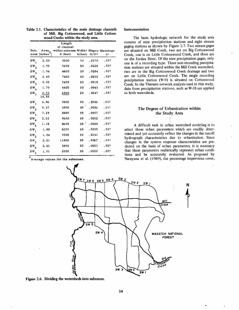
Table 2.1. Characteristics of the main drainage channels of Mill, Big Cottonwood, and Little Cotton­wood Creeks within the study area.

Length of channel

Sub- Area2

within s1.lbzone Width':' Sl'opes Mannings zone (miles ) d (f~et) b(feet) ft/ft"~ n':'

SW1

SW2

SW3

SW4

SWS

SW6

SW7

2.20

1. 95

1. 94

2.49

2.02

1. 70

2..53 14.83

SW1

6.86

SWZ

S.37

SW3

7.Z9

SW4

2.61

SWS 1. 18

SW1

SW2

SW3

SW4

SWS

*

1. 88

1. 94

2.21

2.41

1. 51

92.00

5600

4400

7400

S400

440'b

600,0

9800

3800

8800

9600

8600

8200

3900

11800

3800

2000

30

$0

30

30

~O

30

jo

• P370

.0228

· 0~84

.,OZSO

.0018

.0043

• OO~7

30; • Q586

30 .0036

30 .0057

30 .0052

30 .002'0

~O .0250

30 .0141

3'0 .0067

3'0 .0053

3'0 .• OQ50

Average values for the subzones.

101

!~ ••

~ ~I ~\

.037

.037

.037

.037

.037

.037

.037

.037

.037

.037

.037

.037

.037

.037

·.037

.037

.037

Figure 2.6. Dividing the watersheds into subzones.

14

Instrumentation

The basic hydrologic. network for the study area consists of nine precipitation stations and eight stream gaging stations as shown by Figure 2.7. Two stream gages are situated on Mill Creek, two are on Big Cottonwood Creek, one is on Little Cottonwood Creek, and three are on the Jordan River. Of the nine precipitation gages, only one is of a recording type. Three non-recording precipita­tion stations are situated within the Mill Creek watershed, two are in the Big Cottonwood Creek drainage and two are on Little Cottonwood Creek. The single recording precipitation station (W-9) is situated on Cottonwood Creek. In the Thiessen network analysis used in this study, data from precipitation stations, such as W-38 are applied to both watersheds.

The Degree of Urbanization within the Study Area

A difficult task in urban watershed modeling is to select those urban parameters which are readily deter­mined and yet accurately reflect the changes in the runoff hydrograph characteristics due to urbanization. Since changes in the system response characteristics are pre­dicted on the basis of urban parameters, it is necessary that these parameters realistically represent urban condi­tions and be accurately evaluated. As proposed by Narayana et a1. (1969), the percentage impervious cover,

WASATCH NATIONAL FOREST

N

t

• •

)Wi9 .. • • (

N

eW-37 t

Figure 2.7. Hydrologic instrumentation and the Thieissien polygons for precipitation analysis within the study area.

15

Cf, and the characteristic impervious length factor, Lf, are used in this study as the urban parameters. The values of these parameters are based on physical conditions existing on the watershed at any time, and can be estimated from aerial photos.

Computation of urban parameters

The initial step in evaluating the urban parameters involves the determination of the size of the spatial unit adopted for the model. Narayana et al. (I969) chose the entire watershed as the primary catchment unit. Evelyn et a1. (1970) found that the synthesis of outflow hydro­graphs at selected locations within a basin dictated that a smaller subwatershed or subzone be chosen as the primary catchment unit. The outflows from the subzones are routed and combined to determine the outflow hydro­graph at any specified point. An even smaller unit of spatial area would be the urban block. This unit would permit the synthesis of specific inlet hydrographs for storm drain and gutter design under various assumed degrees of urbanization.

Evelyn et a1. (1970) proposed the following pro­cedure for evaluating the urban parameters, and this procedure was adopted for this study.

I. Divide the watershed into a number of sub­zones as illustrated by Figure 2.6.

A. Factors which influence the number of subzones and their boundaries are: 1. Natural topography and street

configurations. 2. Location of rainfall and stream­

flow gages. 3. Objectives of the study, for ex­

ample, different boundaries might be chosen for investigations in­volving (a) storm characteristics, (b) land use, and ( c) the design of flood control structures.

4. Locations and densities of diversions.

B. The concept of the subwatershed model requires that all outflow from a subzone be defined and preferably be at a single point. The condition of a single outflow point is not essential but it simplifies model development.

II. Determine the impervious cover of roads, buildings, parking lots, and sidewalks. The use of large aerial photographs (in the present study, aerial photos with a scale of 1" = 400' were used) greatly reduces the work involved in that minimal enlargement and tracing of details is necessary. The personnel gathering

16

data can work directly on the aerial photo­graphs, delineating boundaries, subzones, and units within sub zones by means of wax pencils of various colors which can be erased if necessary. Although the areal extent of roads, buildings, parking lots, and sidewalks are estimated separately for each unit con­sidered, the important parameter is the total impervious area. However, the additional work necessary for differentiating between various types of impervious cover often is worthwhile. The separation can provide the researcher or designer with increased insight into the system performance by permitting him to examine the effects of a particular kind of impervious cover on the runoff characteristics of the watershed. In addition, information on various kinds of impervious cover often is needed if other subsequent studies are undertaken, such as an economic analysis. The following procedure is suggested for determining average values of various kinds of impervious cover within a study area.

A. Choose a number of residential blocks so as to include within the sample a representative of each type of block within the watershed. 1. For each block chosen, carefully

measure the precise amount of each type of impervious cover. The total area of the block is considered to be the area enclosed within lines joining the midpoints of the intersections of adjacent roadways (see the dotted en­closure of Figure 2.8). It is sug­gested that linear measurements normally be made with a scale and a rotometer. For large maps or aerial photographs the planimeter also is useful.

2. For each block calculate the per­centage impervious area for each individual type of surface.

3. Average the results of all the blocks to obtain a mean imper­vious area for residential houses. Garage roofs, driveways, and home sidewalks are counted as residential houses. In this study the average area of impervious cover associated with a single resi­dential house was determined by a statistical analysis on the blocks sampled to be approximately 2400 square feet.

4. In the same manner average values are estimated for the widths of residential streets and thorough-

. ) ~ . -- - -'·STREET- ~---+

I

of an urban block indite,ted by ---

CURl a GUTTEu---t+IIII .....

SIDEWALK - ..................

DRiVE WAy---t-t .............

PERVIOUS AREA

PERVIOUS AREA

~-""'I

I t ..............-.--..,

I "'=:...-.1, I ..................... ,

,.---c===t t t::::=:=a I

I a----t t

__._._--t t ==::I J

"""---~ I I

"'---'----' , ~-... J

--=:::r==:=L ...... I I

, -' " t; t---- - --ROAD--------".

)), ( ) (.

Figure 2.8. Typical urban residential block showing the pervious and the impervious areas.

17

fares. Freeways and main high­ways are considered on an individual basis.

B. Divide the study area into units based on the following criteria (Figure 2.9).

1. That the amount of impervious cover and its distribution are near­ly homogeneous within the unit.

2. That the geometric center of the unit can be found from visual inspection. The geometric center is the point from which all runoff from the unit might be considered to originate.

Wasatch National

Forest

Figure 2.9. A sample of dividing subzones into smaller spatial units.

18

c. Analyze each unit within the basin to determine the percentage impervious cover.

1. Using a rotometer estimate the total length of all roads within a unit. This length multiplied by the average road width previously determined equals the area of roadways.

2. Parking lot areas are estimated either by directly measuring their dimensions or by using a planimeter.

v .... · N

III.

3. The dwelling area is determined by counting the number of resi­dential homes and multiplying this total by the average imper­vious area for a single residential home as previously estimated. To this total for dwellings is added individual estimates for larger structures, such as industrial plants, hospitals and churches.

4. The impervious cover for side­walks is obtained by a measure­ment of dimensions. In general sidewalk length can be measured simultaneously with street lengths.

The characteristic impervious length factor is estimated by the following equation (Refer­ence is made to Figure 2.1 0).

L

in which

L = the maximum flow path length within a subzone

L: a i Ii L = ---

m ~ a. 1

in which

aj the impervious area of the ith unit

The paths of drainage usually can be predicted from the conjunctive use of contour and street maps. Quad sheets published by the U.S. Geological Survey in general are adequate for this purpose. In this study only a few field observations of flow at street corners were needed.

8ou.""" ., eO'e' ... " .'0. /-

;> I mp",vj 0 us ____ /_ arC!a, at

,

/ /'

/

/ ,

,

/ I

/ /

/ 'JJIllj Impervious aleOs

aJ • i mpervioUi area

Eo! ::: totol impervious area

to'I' lm=~

Figure 2.10. Sketch illustrating the characteristic impervious length, Lf , for a given watershed or subzone.

19

Summary of calculated urban parameters

The previous discussion has attempted to describe the general method used for determining for a specific study area the two urban parameters of percentage impervious cover an d characteristic impervious length factor. The values of these parameters for the specific urban area of this study are summarized in this section. A sample of the data needed for this determination is shown by Table 2.1 which includes information for only the first urban watershed (SW-l) for the Mill Creek drainage. Most of these data were taken from aerial photographs dated 1965. The raw data were input to a computer program (Appendix B) to provide estimates of (I) The total impervious cover by categories, (2) the characteristic impervious length factor, and (3) the percent impervious cover. The estimates for items (2) and (3) are summarized by Table 2.2.

The figure of 2400 square feet of impervious area for an average urban dwelling was derived by subjectively sampling 21 residential blocks in two urban watersheds. Aerial photographs were used for drawing the samples. For each block mean areas were calculated for the driveway and for the dwelling. On the basis of these individual block estimates corresponding areas were cal­culated for the entire study area. For an average urban dwelling unit a mean residence area of 1833.2 square feet and a mean driveway area of 553.6 square feet, or a total of 2486.8 square feet were obtained. Confidence limits of 95 percent yielded values for the residence between 1716.0 square feet and 1949.4 square feet, and for the driveway between 476.6 square feet and 630 square feet. The upper and lower values associated with these limits are 2193.5 square feet and 2580.0 square feet, respec­tively. As already indicated, impervious areas associated with large buildings, parking lots, and roadways were estimate d by direct scaling from aerial photographs.

Precipitation and Streamflow Inputs to the Hydrology Model

In order to provide for 'the realistic representation of high flow conditions by the hydrologic model, a time increment of one half an hour was adopted. However, the basic precipitation data available are daily totals from non-recording gages and data from recording gages which are published in the form of "Hourly Precipitation Data" by the U.S. Department of Commerce. The daily informa­tion from the non-recording gages was then distributed in time on the same basis as the observed data from the recording gages. This procedure is based on the assump­tion that the time distribution of precipitation is the same at the gaged and the corresponding ungaged locations. It is recognized that this situation might not occur, especially in the case of convective storms.

20

The computed 30-minute precipitation at each gage location is then spatially distributed in accordance with the Thiessen network of Figure 2.7. For illustrative purposes Figure 2.11 shows isohyetal lines and the precipitation station totals for a single storm event. This procedure of spatially distributing point precipitation measurements is generally regarded as being the most accurate, but it is also the most difficult to implement in a computer. In the case of this study some isohyetal charts for specific events were developed and significant differ­ences were not detected between the spatial distributions of precipitation through the isohyetal and the Thiessen weighting methods. Because it is readily implemented on the computer the Thiessen technique was adopted for this study.

Model Verification

The urban hydrologic model discussed previously in this chapter is applied to a particular watershed through a verification procedure whereby the values of certain model parameters are established for a particular proto­type system. Verification of a simulation model is performed in two steps, namely calibration, or system identification, and testing of the model. Data from the prototype system are required in both phases of the verification process. Model calibration involves adjustment of the variable model parameters until a close fit is achieved between observed and computed output func­tions. It therefore follows that the accuracy of predictions from the model cannot exceed that provided by the historical data from the prototype system.

Evaluation of the model parameters can follow any desired pattern, whether it be random or specified. In this study each unknown system coefficient is assigned an initial value, an upper and lower bounds, and the number of increments to cover the range between the assigned bounds. The first selected variable is varied through the specified range while all other variables remain at their initial value. The values of the objective function (measure of error) for each value of the variable are printed, and the value which produces the minimum is stored. After completion of the runs for the first variable, the variable is reset to the initial value and the second variable is taken through the same procedure. After all coefficients have been varied, the set of values which produced each local minimum is run and the resultant objective function value is compared with the smallest attained in all previous runs. The vector which produces the minimum value of the objective function selected as the initial vector is found which produces a reasonable correspondence between computed and observed outflows.

It should be noted that the choice of the variable vector for each phase is based on the judgment and experience of the programmer. However, selection of all variable vectors following the first choice is tempered by the experience gained during the first phase and subse-

Table 2.2. Physical characteristics for the Mill Creek, Big Cottonwood Creek, and Little Cottonwood Creek drainages.

Percent Characteristic Minimum Maximum Hydrograph Length of channel impervious impervious length Depression mfiltration mfiltration rise

Sub- Area2 within subzone Slopes area factor Inte r ception storage rate rate time zone (miles ) d (feet) ft/ft* C f L f SI (In) Sb (Inl F 0 \In/Hrl Fc (In/Hr) tR (min)

Little Cottonwood Creek

SW1

1. 88 8200 .0250 .058 .745 .27 .24 .73 .22 8. 1

SW2

1. 94 3900 • v 141 .120 .535 .25 .21 .71 .22 8.4

SW3

2.21 11800 .0067 .183 .668 .24 .23 .68 .19 9.5

SW4

2.41 ~~OO .0053 .197 .556 .24 .22 .68 .20 10.4

SW5

1. 51 2000 .0050 .048 .667 .27 .22 .71 .21 6.5 9.95 .0172

Big Cottonwood Creek

SW1

6.86 9800 .0586 .118 .623 .26 .22 . 71 .21 29. 7

SW2

5.37 13800 .0036 . 167 .489 .24 .20 79 .21 l5.4 N . - SW

3 7.29 8800 .0057 .117 .438 l5 . 19 72 .22 31. 6

SW4

2.61 9600 0052 154 .401 .24 . 19 .70 .21 11. 3

SW5

1. 18 8600 .0020 .320 .669 .22 .24 .62 · 16 5. 1 23. 31 .0150

Mill Creek

SW 2 20 1

9200 .0370 .262 .477 .22 .21 .65 · 18 9. 5

SW2

1. 95 56,00 .0228 .220 .552 .23 .22 .67 · -19 8,4

SW3

1. 94 4400 .0284 .271 629 .23 .23 .64 · 17 8.4

SW4

2.49 5400 .0250 .026 .690 .28 .23 .75 .23 10.8

SW5

2.02 7400 .0018 250 .682 .23 .24 .S • 1 ~ 8.7

SW6

1. 70 4400 .0043 .273 .638 .23 .23 64 · 17 7.3

SW., 2.53 6000 .0017 .093 .706 .26 23 .7'- .22 10. q

14.83 .0172

* Average values for the watershed channel width =- 30 feet Manning's "n" assumed to equal 0.037.

STORM OF MAY 22-23, 1968

Figure 2.11. Isohyetallines for the event of May 22-23, 1968.

quent phases of the procedure. Thus, model verification effectively uses all previous experience, including that gained during the verification procedure.

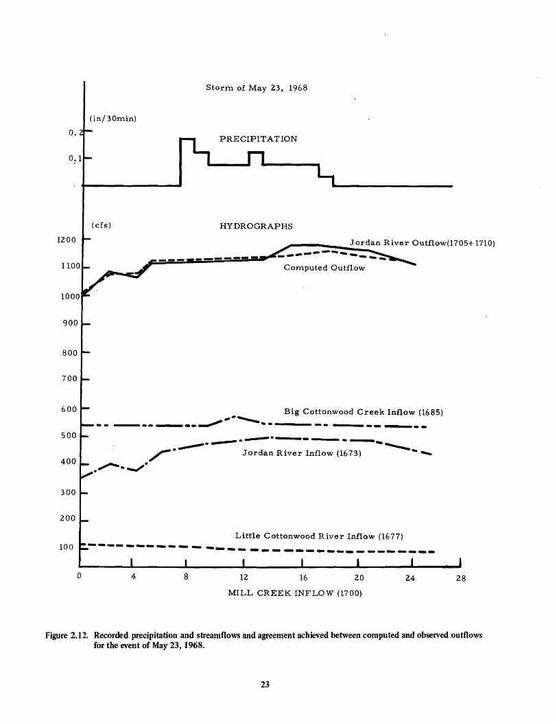
Calibration of the model of this study was based on prototype data from three storms. Model output was compared to measured output by computing the sum of the squared deviations, which became the objective function for the pattern search procedure described previously. The three storms required in excess of 36 solutions of the simultaneous system of equations in terms of water quantities as a function of time. Each of the thre~ storms gave varying values for the five variable parameters. The final value of each parameter was selected objectively to provide the closest agreement between predicted and observed hydrographs for the three storms. These hydrographs represented the total drainage area of the Little Cottonwood, Big Cottonwood, and Mill Creek watersheds. The validity of the model is illustrated by Figure 2.12 which indicates for the event of May 23,

22

V/ASATCH NATIONAL FOREST"

1968, recorded precipitation and stream inflows and the agreement achieved between the computed and observed outflows of the Jordan River.

In order to determine the watershed coefficient values for varying degrees of urbanization it was necessary to establish equations for each parameter based upon the urbanization characteristics. These equations are of the form:

Pm = a + bC f + eLf . . . • • . . • (2.4)

in which Pm represents a model parameter, such as interception storage and Cf and Lf are respectively the percentage impervious cover and the characteristic imper­VlOUS length factor for the watershed or subwatershed under consideration. For a particular drainage area and a

Storm of May 23, 1968

( in / 30min)

PRECIPITATION

(cfs) HYDROGRAPHS

1200 ". __ ~~--~J~o~r.::d:an River Outflow(1705+ 1710)

---------- Computed Outflow

800

700

600 .----.........

------~ ------Big Cottonwood Creek Inflow (1685)

--------500 ---.-._-----....,.,...... ...............

/. Jordan River Inflow (1673) ... -...

."",..... ... ...../. 400

300

200

Little Cottonwood River Inflow (1677) 100 ------------

----~----------------o 4 8 12 16 20 24 28

MILL CREEK INFLOW (1700)

Figure 2.12. Recorded precipitation and streamflows and agreement achieved between computed and observed outflows for the event of May 23, 1968.

23

series of recorded runoff events it is possible to identify through the model calibration procedure values of the model parameter, Pm, which correspond to a range of values for Cf and Lf. In this way values of the coefficients a, b, and c, in Equation 2.4 are found for each parameter included in the model. On the' basis of these relationships it is possible to predict values of model parameters from measured or assumed values of Cf and Lf ·

Streamflow Predictions by the Model

Urbanization in an area generally increases peak discharge and runoff volume, and decreases time to peak discharge. In predicting the flood discharge at different stages of urbanization, available data about streamflow and rainfall recurrence intervals were used to construct

the storm rainfall and upstream inputs. Table 2.3 shows these inputs as they were developed from various sources (Corps of Engineers, 1969, USWD, 1951; USQS 1930-1970, E. A. Richardson, 1971).

With inputs to the model associated with different return periods, and assuming progressive stages of urbani­zation, the model computes the outflow from zone to zone. Figures 2.13, 2.14, and 2.15 illustrate the results of runoff studies for Little Cottonwood Creek, Big Cotton­wood Creek, and Mill Creek. For each creek the runoff was computed for the lowest zone on the watershed or at the confluence of the creek with the Jordan River. For each case, Cf ' the percentage of impervious area was used to indicate the average degree of urbanization on the watershed.

Table 2.3. Precipitation and discharge ranges for various stonn frequencies at the gages indicated.

A. Precipitahon in inches.

Duration 30 mIn. 1 hr. 2 hr. 3 hr. 6 hr. Return Period High Low High Low High Low High Low High Low

2 years .41 37 .52 .45 .62 • 51 .72 .60 .96 .72 5 years 60 .47 .70 .59 .76 .74 .88 .84 1. 23 .95

10 yean .75 .48 .72 .61 .90 .79 .97 .94 1. 40 1. 26 25 years .85 .55 1. 00 .69 1. 10 .92 1. 17 1. 13 1. 67 1. 38 50 years 1. 00 .60 1. 15 .76 1. 24 1. 02 1. 26 1. 26 1. 88 1. 48

100 years 1. 15 64 1. 30 .81 1. 40 1. 10 1. 44 1. 38 2.08 1. 66

B. Discharge in cis.

Creek Jordan River Little Cotton- Big Cotton- Mill Creek Jordan River Station No 1673 wood Creek 1677 wood Creek 1685 1700 1705 & i710

Return Pertod High Low High Low High Low High Low High Low

2 years 900 800 100 50 200 80 50 20 900 600 5 year~ 1300 900 400 150 600 150 100 50 1300 1200

10 years 1700 1000 700 200 900 250 200 80 1700 1700 25 years 2100 1300 1000 350 1200 600 300 150 2500 2100 50 year~ 2400 1500 1200 900 1400 1100 500 300 2800 2400

100 years t700 1800 2500 1400 3000 1500 1400 600 3400 2800

24

2500~----------------------------------------------------------~

2000

~ 1500 u ~

'M Q)

0.0 ,..., co

..c:: u U)

'14 ~

1000

500

Mill Creek, Zone 7

50% 20%

O------~----~--~~--~----~----~----~----~----~----~----~ 10 20 30 40 50 60 70 80 90 100

Return Frequency in Percent

Figure 2.13. Peak discharge vs. return frequency at different stages of urbanization (Cf ).

25

4000

3500

3000

2500

Big Cottonwood Creek, Zone 5

2000

1500

1000

500 50/~

20/~

o 10 20 30 40 50 60 70 80 90 100

Return Frequency in Percent

Figure 2.14. Peak discharge vs. return frequency at different stages of urbanization (Cc).

26

3500r---------------------------------------------------------~

3000

2500

UJ 2000 4-1 U

~ .r-!

Q) 00

""" en ,..c:

1500 CJ UJ

.r-! ~ Little Cottonwood Creek, Zone 5 ~ en Q)

P-!

1000

C f

80%

500 50%

20%

10%

0 10 20 30 40 50 60 70 80 ~O 100

Return Frequency in Percent

Figure 2.1 S. Peak discharge vs. return frequency at different stages of urbanization (Cf ).

27

CHAPTER III

SOME MATHEMATICAL TECHNIQUES FOR MODELING

SOCIOLOGIC RELATIONSHIPS

Introduction

In an urban area the social systems have a prime influence over the characteristics of the hydrologic system because as man builds his various residential areas, business centers, institutions, recrtdtiona1 areas, and other types of development, the characteristics of the function­ing watershed or hydrologic system are modified. In turn, the hydrologic system exerts an influence upon the behavioral characteristics and attitudes of man himself. Thus, in order to predict the consequences of various possible water resource management alternatives in an urban context, it is necessary to understand the inter­acting components of the total system consisting of man and his environment. Chapters III and IV consider the sociological component of the system.

Methodological Approach

In this phase of the study an effort was made, (1) To identify the principal social variables related to urban flooding, and (2) to examine techniques for including the identified variables in a set of mathematical relationships. On the basis of these relationships a mathematical model of the social component of the system was created, which is described in Chapter IV. Field data from a particular location were used to gain a conceptual understanding of the social system, and to test mathematical relationships based on the understanding thus achieved. The various procedures used to obtain the necessary field data, to process these data, and to develop the conceptual frame­work for the formulation of mathematical relationships are discussed in the following paragraphs.

Study Area

As far as possible, data for the sociological com­pon~nt of the model were collected for the study area already described in Chapter I (Figure 1. 1). Notable exceptions were governmental agencies for which jurisdic­tion did not coincide with the physical boundaries of the study area.

29

Data Collection and Identification of Social Varia hIes

A variety of sources were used to provide informa­tion used in identifying sociological variables important for the model. When this project was begun, work was already in progress on defining the elements of the sociological systems for flood control in part of the Salt Lake County area (Andrews and Geertsen, 1973). The survey data from that study were used as basic informa­tion and provided the specific social variables for this fust phase from which preliminary estimates of the values of these parameters were made. The survey materials de­veloped in this preliminary study, and the two samples used which provided the preliminary test data for identi­fying social variables are discussed in the following sections.

Survey data

The survey method has been and is being used to provide information on the populations in order to identify variables associated with flooding or flood con­trol perception. Two specific populations were sampled within the study area that were expected to have some consciousness of flooding decisions. The characteristics that were expected to provide this consciousness were nearness to streams and residence in areas with flooding experience. Therefore, individuals whose residential prop­erties are situated immediately adjacent to a stream (Streamside Sample), and the second strata included individuals situated n,ot adjacent to a stream, but in flood-prone areas which had a history of several floods in past years. In some of these areas, however, no serious flooding has occurred during the/last two or three years.

Initial survey data were obtained by interviewing randomly selected individuals to determine attitudes, felt needs, perspective, perceptions, knowledge, impact of flooding problems, and other factors related to flood control and watershed management. In addition, informa­tion was gathered concerning associated behavior such as opposition to, or support of, flood control proposals or ideas and membership in certain groups. Demographic and other social characteristics of those interviewed were obtained.

Variables examined for potential inclusion within the model are shown in Appendix B. Approximately 130 variables were used in these analyses. Those variables which were found to be significant and consequently which were used in developing the regression equations are shown in Table 3.1. This table also shows the value range adopted in this study for each of the variables. These value ranges represent the minimum to maximum possible values which a variable may have for these analyses, and the particular range is dependent upon the scale used. (This will be discussed further in connection with standardization of measurements.) No particular significance should be attached to the fact that in some cases the lowest value of the range is 0 and in others the value is 1. When appropriate both positive and negative attitudes are reflected by a particular range of values. For example, for J (attitude toward a particular flood control plan) the neutral point is 3, with negative feelings being indicated by values less than 3 and positive feelings being represented by values for J of 4 or 5.

Agency and group data

In addition to data collected by sampling individuals living within the study area, data also were collected from various agencies and groups. Officials and personnel in government agencies dealing with flood control or water management in the urbanized East Salt Lake County area were contacted to obtain information that might be pertinent to the relationships between these agencies and pro blems relate d to flooding within the study area. This was an exploratory attempt to identify forces which affect agency decisions and to begin to evaluate the effects of these decisions. Work in this regard was begun as a part of another study, Project A-010-Utah (Andrews and Geertsen, 1973) and information gathered for the study reported here also augments that of A-O1 O-Utah.

Contacts with public agencies were made in several ways including interviews, letters, and attendance at meetings and hearings. Information was obtained on various factors relate d to the function of agencies such as statements on agency goals, values, and objectives not only as set forth in enabling legislation, but also as these goals or objectives were interpreted and perceived within the internal system of an agency itself. This analysis included the int~rpretations and perceptions of agency administrators since these people directly affect adminis­trative orientation through the influence of their positions which affect agency actions. Information on relationships between agencies and other social systems was also obtained.

Examination was made of relevant parts of federal laws, statues of the State of Utah, and local ordinances. This search was aimed primarily at identifying variables related to the legal parameters of the component organiza­tions to be included in the model such as primary responsibility for flood control, limitations of power, and authority structure.

30

Some of the oth~r agency characteristics for which data were gathered were those related to economic limitations of the agency (funding), the technical capabili­ties of personnel working within the agency, and physical limitations of the agency (equipment and staff available). These factors limit the potential actions which may be taken by the agency itself including the physical actions which may be implemented on a hydrologic system by a particular agency.

Statistical Techniques Applied to Social Data #

Survey data were analyzed by means of several statistical methods, including various non-parametric tests. Chi square, Cramer's V, Contingency Coefficient, and Gamma, a rank-order statistic were used (Nie, et aI., 1970, p. 275-277). The primary objective was to establish the relative importance of each social parameter which had been identified for inclusion as an independent term in various proposed mathematical relationships.

The multiple regression technique

The principal method used in developing social relationships for inclusion in the model was the multiple regression analysis technique. The theory and technique of regression analysis, especially multiple linear regression analysis, is well established in statistics (Freud, 1971; Mosteller, Rourke, and Thomas, 1961; Blalock, 1960), and other applied fields. In the social sciences the procedure has been used most extensively in economics where it is part of the field of econometrics (Wold and Jureen, 1953). tn addition, a number of articles involving regression analysis techniques have appeared in various sociological journals (Blalock, 1968, 1966; Boyle, 1970; Duncan, 1966; Farnessey, 1968; Gordon, 1968).

A short and reasonably simple explanation of the multiple linear regression method is given by engineers Narayana et al. (1970, p. 13), who state that:

The technique of multiple linear regression analysis establishes a functional relationship which predicts the dependent variable from a number of indepen­dent variables. An anticipated relationship is estab­lished, and the least square criterion is applied to empirical observations of both dependent and in­dependent variables solved simultaneously for the coefficients of each term.

Their paper presents a linear mathematical model in general terms and explains how the regression coefficients and constants are determined. In general terms, regression equations are used to formulate causal relationships and to provide predicted estimates on the basis of the causal relationships. For a particular dependent variable, regres­sion equations vary depending upon the availability of data and the degree of resolution required by the problem.

Table 3.1. Variables found important in one or more regression equations and their theoretical ranges as presently measured.

A = Length of residence at present home B = Participation in organizations D = EnvironITIent oriented daily newspaper received

regularly

Range from Minimum to Maximum

0-14 0-31

F = Perceived likelihood of flooding at present residence G = StreaITI proxiITIity

0-1 0-3 1-3 0-16 1-9 1-5 0-1 1-5 0-2 1-4 0-99 1-5 1-5 0-3

°H = Length of residence in local area I = IncoITIe J = Attitude toward a particular flood control plan, J K = Awareness of local flooding problems L = Pe rception of local flood control management M = Marital status N = Rural versus urban ba.ckground o = Occupation P = Attitude toward plan P Q = Condition of horne, yard and neighborhood S = General concern about flooding T = Non-environITIental oriented newspaper regularly

received U = Discus sed flooding problems with others V = Perceived adequacy of local parks W = Flooding expe rienced during lifetime X = Man-made feature beauty score Y = Attitude toward plan Y Z = Natural features beauty score d = Perceived streaITI hazard to children e = Education g = EnvironITIental orientation h = Home ownership i = Knowledge of local governmental flood control

agencies j = Age of individual k = Knowledge about flood control projects p = Political activity score t = Perceived level of local taxes u = Group membership w = Daily newspaper received x = Social class ~ = Promotion of flood control proposal e = Main source of information about flooding A = Attitude toward plan Lambda -y = Membership in flood control group lfJ = Overt opposition to flood control proposal n = Attitude toward plan Omega 11 = With whom discussed flooding problems }.. = Sex ~ = Numbe r of children in family v = Leisure orientation <p = Attendance at flood control meeting or hearing 6. = Knowledge of recent flooding

31

0-1 0-4 1-3 1-4 0-6 1-5 0-6 0-1 0-8 1-5 0-1 0-2

Actual 0-5 0-4 1-5 0-31 0-1

20-134 1-2 0-9 1-5 1-2 1-2 1-5 0-4

0-1 0-7 1-5 1-2 0-1

In exammmg the multiple regression equations which were developed for inclusion in the sociologic component of the overall model, certain variables which had been assumed to be independent appeared repeatedly in several equations. To further examine the role played by these variables, regression models were developed with these as dependent variables. As an example, in some of the preliminary analyses, the variable titled "knowledge of flood control projects" was found to be correlated with the feelings or attitudes of persons toward flood control projects; that is, whether persons favored or opposed particular projects. In order to increase an understanding of those variables which might be correlated with the "knowledge" variable, it also was run as a dependent variable with some of the other variables being used in the independent sense. Through this method of analysis knowledge of interrelationships between variables was increased. Thus, preliminary relationships for the socio­logic component of the model were developed based on conceptual knowledge and testing usin!s field data.

Standardization of measurements

The problem of relating unlike measurements to permit the combining of various measurements into the same equation and the meaningful interpretation of results requires the application of a standardization or weighting procedure. Therefore, mathematical equations in this study are expressed in two forms, deSignated as Forms A and B. Form A includes nonstandardized values, and is based on the scales shown by Table 3.1. For example, the "general concern about flooding," S, is expressed on the basis of a four point scale between 0 and 3, while a five point scale between 1 and 5 is used for "attitude toward a particular flood control plan" J.

The standardized equation form, Form B, is derived from Form A by multiplying the coefficient of each independent variable in Form A by its standard deviation and by dividing by the standard deviation of the depen­dent variable in the equation. The standardized form thus compensates for the differences between the measurement scales used and variations in the distribution of variable values. The standard deviation is used here simply as a measure of variability and not for statistical inference. No particular underlying distribution is assumed, but the values of each of the variables should be reasonably well distributed. This type of technique is discussed by Blalock (I 96 1), Coleman (1966), and Duncan (1966).

The standardized form permits an evaluation of the relative sensitivity of the response of the dependent variable to changes in the various independent variables included in the relationship under consideration. The sign of the coefficient in both forms of the equation indicates the type of relationship, direct or inverse, between the respective independent variable and the dependent vari­able. In the standardized form the larger coefficient associated with a particular variable, the greater is the

32

sensitivity of the dependent variable to variations in that variable. However, this observation does not necessarily mean that the variable with the largest coefficient in the standardized form is the "most important" because its variation may be considerably less than that of a variable with a relatively low coefficient. Under these circum­stances, the variable associated with the lower coefficient might be capable of introducing considerable variation in the dependent variable (Blalock, 1964).

Statistical assumptions

The standardized form of relationships, as discussed in the previous section, is valid and useful provided that the equation is accurate and recursive (Blalock, 1964). Unfortunately, the two conditions of accuracy and recursiveness are not entirely attained with sociological or other social science data. However, these limitations do not mean the technique is inappropriate or inapplicable to social science work providing the user is aware of the limitations and of the resulting approximations (Coleman, 1964). In addition, as the sociologic system is further understood and this increased understanding is reflected in improved data and relationships, it is expected that the two conditions will be met more closely. A further problem associated with the statistical relationships is explained by Coleman {1964, p. 101) as follows:

Other variables which affect the dependent variable are assumed to be uncorrelated to the independent variable, and this assumption is not normally entirely true ... if this assumption is not true, as often it is not, then the observed relation may be a spurious one because of the variables not taken into account. It is to reduce this difficulty that more variables are added and multiple regression is used.

Two other assumptions mentioned by Coleman (1964) are: 1) the structure of the equations is theoretically correct; that is, that the independent variables are causally related as described by the equation to the dependent variable; and 2) the parameters of the equations are alike or nearly so for all units in which observations are made. The second assumption is often met in sociological samples drawn from the same population. Meeting the first assumption requires a knowledge of the system being studied. I

I

For the present, relationships within the sociologic component of the system are assumed to be linear because of the resulting ease of representation and analysis and because the system is not sufficiently well defined to permit other than this assumption. As defined, a linear regression equation is one in which changes in the dependent variable are constantly proportional to changes in each of the independent variables; a linear relationship between two variables can be represented as a straight line. The linear hypothesis is a first approximation. Since the relationships of some important social variables in the hydrologic-sociologic system may not be linear, efforts will be made in the future to gain further knowledge of

the real world, and thus to improve the accuracy of the equations in the model.

One frequently stated requirement for linear regres­sion analysis and related statistical techniques is that interval scales are needed although multiple regression can be run using categorical predictors. This implies the measurement of variables using a continuous number system where differences between values of variables are quantified. Recent investigations have shown that power­ful parametric statistics are useful even when scales do not meet all of the assumptions for the statistics. Sanford Labowitz (1967, 1971; also Baker, 1971) demonstrated that even radically different numbering systems for ordinal data do not greatly change the results when statistical techniques normally requiring interval scales are applied to constructed interval scales. He wrote:

Empirical evidence supports the treatment of ordinal variables as if they conformed to interval scales. Although some small error may accompany the treatment of ordinal variables as interval, this is offset by the use of more powerful, more sensitive, more highly developed, and more clearly interpre­table statistics with known sampling error. For example, well defined measures of dispersion (vari­ance) require interval or ratio based measures. Furthermore, many more manipulations (which may be necessary to the problem in question) are possible with interval measurement, e.g., partial correlation, multivariate correlation and regression, analysis of variance and covariance, and most pictorial presenta­tions ... (Labowitz, 1971, p. 515).

For the purpose of this study, the specification of important variables and the general nature of their relationship, the data have been formulated and treated as interval information. This is the reason why dummy variables are not used in the regression equations with ordinal data; the data are treated as if they measured the underlying variable continuously. It is expected that with additional study, methods of measurement will be im­proved to more closely approximate interval scales in the real sense.

Social applications of regression analysis

In a recent sociological study, Chase (I 968) applied regression analysis to examine the effects of aggregate economic growth on unrelated individuals. Coleman et aI., (1966) describe a model which uses regression equations for expressing equality of education opportunity. Regres­sion techniques are used by Gaulle and Trauber (I 966) to describe the relationship of opportunity and metropolitan migration. Hamblin and Smith (1966) refer to a special­ized application of the same techniques for a student evaluation of the status of professors in accordance with several factors.

Many other interesting and useful sociological appli­cations of the linear regression analysis have been made. One of these describes a linear model for determining the relationships between demographic factors and the

33

education-labor force system (Frigyes, 1968). An unusual application of regression analysis was made by White (I969) when he used this technique to analyze the migration to and from enclosed cities during the 18th and early 19th centuries. An extremely useful application of regression analysis was made by Anderson (I 972) when he applied this technique to analyze the health care system of the State of New Mexico. Simon (1968) used time series regression analysis in which time is treated as a controlled variable, to explain seemingly contradictory results in earlier articles on the effect of income on the suicide rate. An example of the joint application of simulation and regression analyses is a model which predicted, quite accurately, the outcome of the 1964 presidential election in Missouri (Lynch and Engberg, 1967).

Techniques similar to those used in the studies mentioned in the preceding paragraphs were applied in this study to: 1) identify important variables; and 2) develop equations for the sociologic component of the model.

An Example of the Development of a Sociologic Regression Relationship

In order to provide the reader with a clear explana­tion of the manner in which multiple regression tech­niques were applied in the development of sociologic relationships, a specific example for one dependent variable is briefly described.

The dependent variable used in this example is the "perceived likelihood of flooding at present residence" (variable F in Table 3.1). This variable is designed to indicate the public perception of flooding probabilities by the popUlation included within the area of this study. The value of F is based upon responses to the interview question: "In the next five years what do you feel will be the likelihood that you will experience flooding at your present residence: none, low, moderate or high?" The information on this question was taken from people living along streams and in areas with a flood history. At the time of the interview there was no imminent danger of being flooded. Persons in imminent danger of being flooded would be expected to have a different perception of the situation.

Results of the analyses indicate as expected that an individual's perception of the likelihood of flooding at his residence is an important motivating variable. Officials in the Salt Lake County Flood Control Department reported that persons who perceived that they were in danger of being flooded often called the department for relief action. Thus, F appears to be an important variable to include in the model as agency input from the public. If persons in imminent danger of being flooded had been included in the survey to provide data, the importance of this variable could be expected to have been even greater. This variable, F, was found to be important not only as a

motivator in the model, but also because of its relation­ship with several other types of social behavior including promotion of or opposition to flood control projects.

As can be seen from the lists in Table 3.1 and Appendix B, a variety of variables were included in this particular questionnaire and tested for Significance and relationship to the perceived risk of flooding. Those dependent variables that seemed promising were subse­quently included in the multiple regression analysis.

Some of the independent variables included in the first step-wise multiple regression runs for the dependent variable F were the following:

1. Perception of local flooding control management

2. Flooding experienced during lifetime 3. Home ownership 4. Area of upbringing 5. Leisure orientation 6. Social class 7. Marital status 8. General concern about flooding 9. Main source of information about flooding

10. Relative damage received from flooding 11. Pleasure received from the stream

The analysis indicated that of those tested the following four independent variables are the most signifi­cant in explaining variations in F:

1. General concern about flooding, S 2. Flooding experienced during lifetime, W 3. Perception of local flood control manage­

ment, L 4. Main source of information about flooding, e

These four independent variables, therefore, are being used to predict the variation in intensity of feeling about probable danger of flooding as shown in the dependent variable, F, "perceived likelihood of flooding at present residence." The measure of these variables used for this initial analysis is described below.

Description of the independent variables

The independent variable, S, in this case study is based on the question: "What would you say is the degree of concern or worry that you have about flooding; none, low, moderate, or high?" In this example "perceived likelihood of flooding at present residence," F, is being treated as a dependent variable. As might be expected, there is a strong correlation between F and S, and for this reason they do not both appear as independent variables in any of. the same regression equations developed for the sociologic component of the overall model.

I t should be noted that when close correlations exist, the causal relationship needs to be hypothesized. The correctness or incorrectness of the relationship hypothesized will usually become increaSingly apparent as the whole system is analyzed in a model. Corrections for

34

this as well as other things can be expected to be made as the model building process continues.

The second important independent variable listed above is W, "flooding experienced during lifetime." This particular variable takes into account whether a re­spondent had previously experienced damage or incon­venience due to flooding, and if so, whether this experience had occurred within the study area. This is obviously related to the hydrologic system since this situation is more likely to occur with increased frequency of flooding, a function of the hydrologic system. For the regression analysis involving this variable four alternatives were considered:

1. The individual had not experienced damage or inconvenience due to flooding at any time during his lifetime.

2. The individual had experienced damage or inconvenience due to flooding only outside of the study area.

3. The individual had experienced damage or inconvenience due to flooding in the study area but not in his present home.

4. The individual had experienced damage or inconvenience due to flooding in his present home within the study area.

These alternatives are ordered according to the degree of proximity of flooding experience to the individual's current residence.

The relationship between the dependent variable F and the independent variable W is positive. Thus, those who had been flooded in their present homes had a greater tendency toward a high "perceived likelihood of flooding" as compared with those who had been flooded elsewhere. The variable W also is capable of providing some insight into a' "crisis situation" in which the homes of residents are being flooded or are in imminent danger of being flooded. In this particular situation an indi­vidual's perception of the "likelihood of being flooded" to some degree will be influenced by his previous experience, as indicated by W; in other words, he is more likely to perceive a situation as a real threat, the more he had experienced the problem. For example, an official of the Salt Lake County Flood Control Department ex­plained that his department is contacted more frequently by those who have experienced flooding previously than by those who have not. The independent variable, W, is identified as being important in explaining variations in F, the perceived likelihood of flooding at the present residence.

The third independent variable identified as being important in this example relationship is L, "perception of local flood control management." This variable is based on a composite attitude score by individuals toward the following items related to flood control in the study area:

1. Seriousness of flooding in the local area 2. Attitude toward emergency flood control

work

3. Whether flooding is presently a problem in the area

4. Whether something should be done to control flooding problems

5. Factors contributing to flooding in the local area

The attitudes of those samples on a scale from one to five were obtained in relation to each of the items and then an average scale score was calculated.

. The fourth independent variable, 8 , "main source of information about flooding," is intended to reflect the effects of information sources on the dependent variable, F. The various types of information sources given by those interviewed are ordered according to how primary or close to the individual the source is and are as follows: 1) had not heard about flood control projects in the study area during the past year or so; 2) television or radio; 3) newspapers; 4) an official source such as a county employee; 5) public and private meetings; 6) work associates; 7) friends not in the neighborhood; 8) friends in the neighborhood; 9) family members; and 10) personal observation.

The general equation

Although in some cases the important determining causes of a particular variable such as F above can be ascertained by methods other than that described here, the relative importance of such factors cannot generally be obtained nor can the multiplicative effect of a change in one variable in a system often be easily determined. One value of an equation is in determining the relative importance of the causal factors (see section on standard­ization, p. 32). One value of modeling a system on a computer by use of a set of equations representing the system is that the possible compound effects of change in one variable can be seen elsewhere in the system through the simulation process.

In this example, four independent variables are identified as being important for inclusion in an equation for predicting the dependent variable, F, the perceived likelihood of flooding at present residence. Thus, one dependent and four independent variables are included in the equation which is as follows:

F = b + b S + b W + b L + b 8 . • . . (3.1)1 o S W L 8

1Technically speaking, an equation of form 3.1 would also have an error variance term for the unexplained variation in the dependent variable. However, here the equations are used to represent relationships between variables. Generally, an inde­pendent variable was retained if it explained about 1 percent or more of the r2 or in other words, the variance of the dependent variable in a regression equation. In many cases the contribution to r2 was considerably larger than this. An F significance test was used in the computer in selecting the most important independent variables for regression analysis.

35

in which

Range F = perceived likelihood of flooding

at present residence 0-3 S = general concern about flooding 0-3 W = flooding experienced during

lifetime 1-4 L = perception of local flood control

management 1-5 8 = main source of information about

flooding 0-9 bo = the intercept

The other constants, "b" in the equatio~ designate coefficients determined by the regression analysis for each of the independent variables.

For a simulation problem values may be estimated and assigned or actual data used. This data may then be varied as desired to observe the effect of change on the problem. Subsequent to calibration, studies can be con­ducted to examine the sensitivity of the response function (values of the dependent variable) to changes in the value of the various independent variables within the ranges of these variables.

Improvements are done by calibrating or making adjustments from additional or better data so as to match predicted results with actual results. As is the case for models of physical systems, calibration is bas~d on field data. The general regression relationship of Equation (1) requires calibration by adjustment of the constants for each study area to which the equation is applied.

The general procedure described in the foregoing section can be utilized in the development of all regression equations proposed for the sociologic components of the overall model.

Stratification of sociologic sampling

As previously mentioned, sociologic data in this study were drawn from two samples of respondents within the study area, namely (1) Streamside sample, and (2) the flood damage area sample. Regression equations were developed for each of the two samples. A subscript of "s" on the dependent variable in the equations indicates that the information used in developing the equation came from the streamside sample only, while a subscript of "f" designates that only data from the flood damage sample were used. Equation (3.1) for each of these two samples appears as follows:

Form A (non-standardized):

Ff= -.65 + .13L + .• 059 + .27W + .37S ...

F.:' -.77 - .058 + • 12W + . 30L + .49S. . . ef

(3.2)

(3.3)

Form B (standardized):

F f = -.65 + . 10L + . 158 + .41 W + .415 . . • (3.4)

F~ = -.77 - • 148 + • 16 W + • 25L + .495. . . (3.5)

Sometimes it was useful for experimental purposes to combine the information collected in both samples because of the lack of adequate numbers of people in particular categories in the separate samples. In these instances the subscript "c" was applied to the dependent variable, This particular technique was not needed in the case of perceived likelihood of flooding at present residence, F.

Differences in the coefficients within the equations above for a particular form (A or B) reflect differences in the two sample locations. This indicates the type of adjustments of the relationships necessary to apply the equation to different types of populations. For each study

36

area (or identified subzone thereof) the equation is calibrated by means of data from the area under consider­ation. In the case of F the same four independent variables were identified by both samples as being the most significant in the relationship (Equation 3.1). The perceived likelihood of flooding at present residences is an important mathematical formulation in the entire socio­logic component of the model las described in the next chapter.

This same regression technique is used to obtain the social functions that were developed that are included in the model. The principal purpose of the equations derived from the regression ana1ys~s was to identify as well as indicate the relative importance of these variables to the respective dependent variabies. However, two other types of equations, those that Jre logical representations of agency processes and thJse that show how general relationships are formed, are also used in the model. The general relationship represented by Equation 3.1 will again be referred to in Chapter IV wherein the equation will be placed in context with other relationships included within the sociologic component of the model.

CHAPTER IV

IDENTIFYING THE COMPONENTS OF THE SOCIOLOGIC ACTION PROCESS SUBSYSTEM

In order to explore the development of a mathe­matical model of the sociologic flow system it is necessary to make an identification of the basic elements of the system and to investigate the linkage functions between the inter-connected components of the system.

As discussed earlier, the development of a mathe­matical model consists of two major steps, namely (1) A conceptualization of the system (or system identifica­tion), and (2) the formulation of mathematical representa­tions of the various processes identified in Step 1. The conceptual model of the hydrologic-sociologic flow system in the context of urban flooding as developed under this study is shown by Figure 4.1 .

A Conceptual Model of the Hydrologic-Sociologic Flow System

Figure 4.1 includes in conceptual form the broad subsystems represented by the preliminary flow chart of Figure 1.3. Even in Figure 4.1 complex relationships existing in the real world are necessarily simplified, and this flow diagram provides a skeletal representation of the flow from one behavioral process' to another and the linkages between the hydrologic-sociologic components of the system. Included in the figure are many widely varying processes which occur in both the physical and the sociologic worlds. The behavioral processes repre­sented are those of agencies, individuals, and other social systems. The flow 'diagram illustrates interactions of various agencies with each other as well as the actions and reactions of the public (both individuals and groups). It is likely that additional processes will be added with a further understanding of the system.

Difficulties were encountered in identifying and modeling some of the social components shown by this diagram. Figure 4.1 represents a tentative model. As further insight into the system is developed, blank spots that may exist in the conceptual model of the real world system will be discovered and compensatory adjustments made in both the conceptual and mathematical models.

Following the development of the conceptual model, the problem then became one of formulating appropriate mathematical relationships for the various processes represented by the diagram of Figure 4.1. The

37

procedure used for doing this was the subject discussed in Chapter III.

Figure 4.1 is divided into six stages or sections. The model as re presented by these sections are (1) The state of public opinion information and perception of flooding problems, (2) planning agencies or social structure for planning activities and the preliminary proposal process, (3) decision agencies or structure for analysis and adop­tion of the proposed plan, (4) public reaction acceptance, adjustment or rejection process, (5) alternative actions subcycle, and (6) implementation of actions. The six sections provide an organizational framework for the development and discussion of the model. Each section will be examined, and the various basic elements and processes which were identified as being a part of each will be discussed. It should be remembered that the processes described may result in looping back to a previous section at almost any point in the process; this is shown in Figure 4.1 by the returning arrows. Preliminary mathematical equations representing some of these processes for use in the model are developed. Finally, the flow chart only describes a process and its elements. There may be much overlapping of functions and several functions occur simultaneously in the various systems. For example the same agencies often perform the func­tions of planning, decision, and action. However, the action and components in the process remain the same.

Section One: Public Opinion

A two stage screening process was described in Chapter III which (1) Identified related variables and (2) indicated those variables which were considered most important in predicting behavior and attitudes in relation to modification of the hydrologic system. Those more important variables are treated as primary dependent variables while several related variables are treated as independent secondary terms in regression analyses to form a predictive equ~tion for each of the important primary dependent variables.

Terms in the equations provide a transition from one stage to another with a dependent variable in an equation of a preceding stage becoming an independent variable in another equation. This represents a direct effect of that variable upon another independent variable in the model and is one way that the linkage of the system

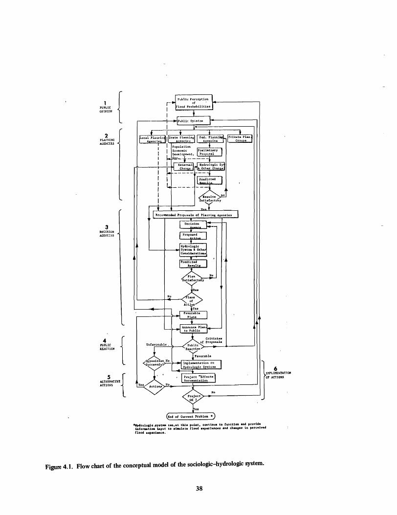
PUBLIC { OPINION

2 PLAl"~n~G

AGENCIES

3 DECISIO!l AGENca:s

4 l'IIBLIC IlEACTlON

}1!!!'LI~""'l'AT[OH OF ACTIONS

>-~----------------~

*IIJcIrolo.ic .. ,at •• c:c,at tbi. poiot, c:outioue to func:tioo aDd provide iofo .... U ... ioput to as...late flood e"Puteroc •• end c:hao," 1n p.r~e1ved flood expu.lenc8.

Figure 4.1. Flow chart of the conceptual model of the sociologic-hydrologic system.

38

is represented in the model. Linkage of the various parts of a system permits the effect of changes in any element of the system to be seen at any point in the model. Analysis of complex causal relationships can thus be done to the extent that the model simulates reality.

In the search for variables associated with flood control behavior, the field study provided several variables pertinent to the public opinion section of the flow chart.

Public perception of flood probabilities

One of the central variables found to be of importance to behavioral action in the public opinion section of Figure 4.1 is that which was used in Chapter III to illustrate the analysis methodology; namely, that of perceived likelihood of flooding at present residence, F. This social parameter is used as a dependent variable, and thus is expressed in terms of specific independent vari­ables which were identified and measured through survey techniques. The independent variables which were examined in relationship to F and found to be of most importance in explaining its variability are:

1. General concern about flooding, S. 2. Flooding experienced during lifetime, W. 3. Perception of local flood control manage­

ment, L. 4. Main source of information, 8.

A mathematical representation of a relationship which contains these four variables is given by Equation 3.1, and is repeated here as follows:

F := bo + bS

S + b w W + bL

L + be e .. (4.1)1

in which all variables are as defined above. 2

The output for this particular section of the model is the function, F, which is an input to the second section of the model, namely, Planning Agencies.

It is realized that the existence of an attitude without any associated overt behavior by members of a population may exert little influence on a planning agency. Under these conditions it is probable that the agency would have no way of knowing that such an attitude exists. In the case of F, however, experience within the study area has shown that whenever people perceived that the likelihood of flooding at their residence was high they tended to call the local Flood Control Department to request some form of flood control action. F appears to be an important motivating variable, also

. 1 See footnote, Chapter III, p. 35).

2Reference is made to Chapter III for the operational definitions and discussion of these variables.

39

related to other types of action behavior such as member­ship in citizens groups and other organizations which are mainly interested in flood control projects. Groups of this type are capable of strongly influencing agency behavior. Because of its demonstrated functional centrality, the variable F is used in the model as a behavioral link between the public and various agencies. The use of a central variable such as F helps to simplify the representa­tion of processes within the mathematical model.

Concern about flooding

One of the important independent variables men­tioned in connection with F (perceived likelihood of flooding at present residence) is "general concern about flooding" S. This parameter was examined as a dependent variable to determine what factors can be used to explain this "concern." The following variables were found to be useful in this regard:

h home ownership K awareness of local flooding problems B participation in organizations

age of individual

Variables occur at several levels. First, primary dependent variables such as F or S are used here. Second, secondary or independent variables' which are causal to or explain the variance of the primary dependent variables.

The first of these related variables, "home owner­ship," h, is dichotomous; that is, either the home is owned or being purchased, or it is not. For the sample within the flood prone area, S was found to be higher for persons who were buying or who owned their own home than for those who did not. In general the degree of concern for flooding is expected to be positively related to home ownership. However, for the streamside sample, an inverse relationship was found between the ownership of homes and the general concdrn about flooding. This can be partially explained by comparing differences between the samples. Perhaps the persons who lived along the stream bought there because they were less concerned about flooding than others who were not buying there (a self-selection process). Another possible explanation is that if persons buying or owning along streams had ever felt a concern for flooding, after several years with no serious flood experience, they have lost this concern or they may have rationalized away their concern in order to reach a state of consonance rather than to continually have a state of cognitive dissonance (Fe stinger , 1957) in relation to the stream and its flooding potential.

The relationship between "awareness of local flood­ing problems," K, and S is positive. K was estimated by determining whether individuals in the population had heard about flood problems or flood control projects in the previous year. As would be expected, "participation in organizations related to flooding," B, was identified as having a positive relationship with S. The higher the

participation, the higher the general concern about flooding.

The "age of the individual," j, also was found to be relate d to "concern for flooding." This relationship was inverse or negative in that the older the person, the less his concern for flooding, and the younger the person, the higher his'concern about flooding.

Using the four independent variables discussed above, a general equation for concern for flooding, S, is as follows:

in which all terms are as previously defined.

It is possible that other variables may need to be included in the equation for genera] concern about flooding, S. For example, the influence or relationship of "expert" opinion about flood probabilities, problems, and solutions. If it is assumed, in this instance, that there is a direct relationship between expert opinion about flood probabilities and concern about flooding, then if expert opinion is predicting flooding or that there is a high degree of flood probability, the concern about flooding in general will increase. An increase in S would produce an increase in F in accordance with Equation 4.1. Thus, as water management agencies go through their decision processes and evaluate various alternatives for flood control, the actual flood control danger as perceived by each agency can cause a corresponding increase or decrease in the perception of the probability of flooding by the population. Changes of this nature, in turn, will influence the pressure exerted by the population on the agencies to plan or to implement flood control measures.

Flooding experienced during lifetime

The second independent variable in Equation 4.1 is concerned with past flooding experiences or W. The value of this parameter is influenced by both spatial and temporal variations. Spatial variations occur with respect to the location of previous flooding experience. The value of W is higher for individuals who have experienced flooding at their present residences than for those who have experienced flooding elsewhere, but not at their present residence. Temporal variations in W occur as a result of changes in potential flood danger. The mean value of W should vary directly with the flood probability of a given area which may change over time due to direct actions (i.e., a flood control measure or changing conditions).

The experience parameter, W, provides a link or connection between the hydrologic and the social com­ponents of the system. Output from the hydrologic system influences the value of W which in turn produces changes in F in accordance with Equation 4.1.

40

Other secondary variables

The remaining two independent variables in Equa­tion 4.1, namely Land 8 , have not been examined in this study in terms of secondary or contingent variables. A further "breakdown" in this respect could be performed in a subsequent analysis, only magnitudes of Land 8 have been established here.

Summary

Public opinion, in the preceding discussion which is designated as Section 1 in Figure 4.1, is related to various measurable social parameters. Public opinion is associated with urban flooding and the process of flood control. A relationship is proposed (Equation 4.1) which predicts perceived likelihood of flooding at present residence, F, as a function of four identifiable and measurable parameters. In the model as now proposed the output of Section One is the value of F which is the main input to Section Two. However, as noted earlier, the model is in the develop­ment stages, and it will be expanded and altered as conceptual understanding of the system is increased.

Section Two: Planning Agencies

The second section of the model shown by Figure 4.1 is an analysis of the processes and components of the conditions of urban social and hydrologic systems and the formation of a plan or recommended solutions for solving a problem or problems in that system.

The discussion of the manner in which various aspects and functions of planning agencies concerned with flood control are considered in the model is divided into three major parts: (1) A consideration of some of the characteristics of the various planning agencies involved with flood control problems with the study area; (2) a discussion of the manner in which planning agencies identify and evaluate flooding problems; and (3) a consideration of strategies used by agencies for identifying solutions and for evaluating the results of the decision­making processes. An attempt is made to identify im­portant social variables and relationships for inclusion in this section of the model.

Characteristics of planning agencies

Particular attention was given to the examination of the processes of planning and implementing policies affecting the hydrology of the watershed and the factors controlling these processes. State law provides that the county gowrnment and agencies within that government have prime decision power on flood control activities in the study area. It is true that many diverse individuals and groups hold property rights in the watershed being examined. However, through various rules and regulations

and potentially the use of the right of eminent domain and condemnation, the county and agencies within the county government hold great power. Therefore, in the area of the field study, the county government has the greatest power in controlling what happens to the hydrology of the watershed. The main county agencies involved are the County Flood Control Department, the County Planning and Zoning Department, and the Board of County Commissioners.

Through its enabling legislation, the Salt Lake County Flood Control Department has been given the charge to "assist the Board of County Commissioners in the discharge of the responsibility for the gathering, control, and disposal of storm drainage and flood water, for the conservation of such water for beneficial and useful purposes, and for the protection of personal property, public highways, and waterways within the county from damage resulting from such water." The ordinance further states that the department "shall administer all County ordinances pertaining to flood problems" (Revised Ordinances of Salt Lake County, Section 7/2/1). Thus, the County Flood Control Depart­ment has broad responsibilities which fall within the interest and scope of this project and holds major power in water control related activities in Salt Lake County. Because of this power, the Flood Control Department is represented in the model as being the principal agency related to flood control.

The Salt Lake County Planning and Zoning Depart­ment, which in water related issues works with the County Flood Control Department, has authority to control modifications on the urban watershed included in the study. Watershed characteristics, such as the degree and rate of urbanization, are greatly affected by decisions of the County Planning and Zoning Department.

The two agencies, the County Flood Control Department and the Planning and Zoning Department, together with the supervision that they receive from the Salt Lake County Board of Commissioners, provide the major sources of decisions for changes that will be implemented on the urban watershed currently within the study area. Under the existing ordinances of the county and also under the rules surrounding the operation of these two agencies, they work in close cooperation in reaching many of the decisions affecting the area being modeled. For example, problems related to drainage within subdivisions are discussed jointly before decisions are made since the County Flood Control Department is represen ted at meetings concerning proposed construction within Salt Lake County. Because of this close coordina­tion, the county government can be and is treated as a unit; neither the County Planning and Zoning Department nor the County Board of Commissioners is represented separately in the current prototype model. The construc­tion of the model permits the introduction of divisions of this nature as needed in subsequent development of the model.

41

The supervisory role played by the Salt Lake County Board of Commissioners is of prime importance since the board can provide not only planning and direction, but may also change the characteristics of the decision agencies themselves. In the future the Salt Lake County Board of Commissioners may be included separ­ately as a powerful input agency to other functioning county decision agencies within the area. In addition, at the local level, other municipal commissioners, mayors, and associated agencies can have input and may be considered.

Other social systems at the federal, state, and local levels have an input into the decisions made within the county. However, for conceptualization within a com­puter type model, these agencies may be viewed as acting primarily in a planning capacity while the county has the major decision power on what policies are implemented. By using this conceptualization, the model becomes simpler and does not consequently represent as many as possible of the in teractions and interrelationships which exist. However, for the purposes of simulating social processes as related to the hydrology of a watershed, this simplified view may be adequate for the present and will hel p in developing the simulation model.

Several agencies can act in a planning capacity. On the federal level the Army Corps of Engineers has a major role to provide plans to be implemented. Other federal agencies such as the Forest Service can be included in the future when appropriate.

Provision has also been made in the model to consider potential inputs from private groups and con­sultants. An example is the master storm drainage plan designed for the Salt Lake County area by a private engineering firm which was engaged by the county's Flood Control Department. Various other plans relating to flood control also have been developed by other professional engineering firms. In addition, the influence of various private citizen groups on the planning function can be included in the second section of the model. However, their effects are included further on in this prototype model.

Agency relationships which affect the planning process. In order to determine the functional role of the various agencies in the planning process, several character­istics were examined which involve relationships between agencies and between agencies and other organizations, groups and individuals. Included within these relationships were factors related to social power or the sensitivity of a particular agency or social system to social forces coming from outside the agency or system.

The power of an agency encompasses authority and influence. Authority is power intrinsic to the agency itself, and this power is related to the accomplishment of tasks which the agency has been assigned. Influence is the ability of an individual or agency to affect the behavior of

other agencies, groups, or individuals in areas not directly under the authority of the agency. An example of the function of these two types of power may be illustrated by the way agencies behave with regard to a problem. For a problem in Salt Lake County, the County Flood Department has the authority to decide whether a particular control method will be applied or not, but another agency that has resources, either technical, financial, or other, may, by withholding its resources or by involving expert advisors or other means, be able to affect. the decision made. This ability to effect a decision indirectly is equally as important a type of power as authority.

Power relationships can greatly affect the behavior and function of an agency. The sources of the issue and the other social systems affected by or acting in relation to a particular problem need to be considered as this will in turn influence an agency's action. Potential adverse action by other social systems may be considered, including anything that is perceived by agency adminis­trators as a potential adverse action. Perceived advantage for the agency is another factor which may affect the behavior of the agency or social system.

Agency actions also are influenced by agency administrators who may view exactly the same thing or set of conditions in different ways. For this reason, an effort was also made in this study to obtain information on the perceptions held by the various agency adminis­trators and the stated policies of the agency.

Steps in the decision processes of planning agencies. Mter examining planning agencies in the study area, several of the steps in their decision processes were identified. These are shown by Table 4.1. The order of the steps may not be in a specific sequence. The important points identified by Table 4.1 are: (1) The important factors determinative of agency action, and (2) that all important factors must be positive to some degree for the action to occur. Resolution of problems will occur if the factors are such that no function is negative; otherwise no action or an alternative action will occur.

Inherently included within the process are the kinds of agency controls and constraints, both internal and external, which are discussed briefly in the previous section of this report. Internal constraints are due to the characteristics of the agency, and external constraints are provided by information inputs from other social systems and by existing relationships with these other systems. The social power is important since a strong external influence can greatly affect the decisions which are made by a particular agency.

An examination of the steps outlined by Table 4.1 iden tifies some of the basic relationships or functions needed in the model. For example, the decision process involves the follOwing six functions:

42

1. Flood control 2. Cost and other economic factors 3. Aesthetics 4. Recreation 5. Acceptance of an action by other agencies 6. Acceptance of an action by relevant

populations Each of these functions will be defined and discussed in subsequent sections of this report which deals with solution recognition and evaluation.

Identifying and Evaluating Planning Problems

In the model represented by Figure 4.1, the section titled "Planning Agencies" includes a representation of functioning bureaucracies whose miS'sions are to define problems and prepare solutions related to urban flooding problems. These functions are performed within the limits of their organizational characteristics and responsibilities. An agency may be alerted to a flooding problem by either the hydrologic component of the model directly or by the public perception of flood probabilities. In the model the public perception of flooding probabilities is the value of F, perceived likelihood of flooding. Under normal con­ditions an agency will continue to search for flooding problems and to make evaluations of the conditions of the hydrologic system within the limits of its own character­istics unless the public value of the F input from Section One reaches a level to which the agency will react. This is because it is characteristic of any bureaucracy to locate work which will allow the bureaucracy to maintain its existence at past levels or more; and this work must be within the prescribed limits, legal and social, of activity of the bureaucracy.

The pressure exerted through public opinion may be varied, and this is reflected in the value of F. When the value of the F input is above the level to which an agency will react, the agency will search for solutions to specific flooding problems in the hydrologic system causing the high level of F until F is lowered. The value of F may be low:ered, for example, through feedback of "expert knowledge and opinion" which indicates a less serious flooding condition than that which might previously have been supposed. The lowering of F also can be accom­plished through the implementation of an action to alleviate flooding conditions and by the subsequent feedback of this information from the hydrologic system (present condition of the physical system) to the Public Opinion section of the sociologic model.

It is the function of some agencies and organizations to provide solutions to flooding problems as well as plans for flood control. This type of agency will continue to search for flooding problems regardless of the value of F. An example of this type of agency is the previously mentioned County Flood Control Department whose responsibilities include water control and avoidance of damage caused by flooding. However, the value of F still influences the decisions and behavior of this agency.

Yes

Emergency Actions

(same as 112 )

Yes

(113)

Yes

(117)

Yes (any conflicts)

Yes

PROBLEM

No

Non-Emergency Actions

Technologic feasibility

Potential control

Futur~

control potential

Economically feasible

Aesthetic recreationally feasible

Best solution for conditions

No conflict key agencies

No conflict other agencies

No public conflict

RECO~WffiNDATION OR IMPLEMENTATION

Decision Blocks Are Explained by Figure 4.3

Figure 4.2. Identified important steps or components of the agency decision process.

43

Table 4.1. Explanation of decision blocks shown by Figure 4.2.

Decision blocks:

1. Is emergency action needed to protect en­dangere d property, person, highways, waterways?

2. Can the agency technologically implement the action?

3. Will the action provide a solution to the flooding problem (flood controlling potential)?

4. Will the action prevent future problems (flood controlling potential)?

5. Is the action economically possible?

6. Is the action possible from aesthetic and recreation standpoints?

7. Is the action the best usable solution under existing conditions?

8. Is action in harmony with the key authorizing agency, i.e., no action-blocking conflict with key government authority exists (perception of acceptance by other government agencies)?

9. Is action in harmony with other agencies, i.e., no action-blocking conflict of other govern­ment agencies exist (perception of acceptance by other government agencies)?

10. Is action in harmony with the public, i.e., no action-blocking conflict from the population exist (perception of acceptance by the pUblic)?

EmergenCy actions:

11. Can the agency technologically implement the action (is it possible from a technological standpoint)?

12. Will the action protect property, person, highway, waterway for the emergency period (flood controlling potential)?

13. Is the action the best usable solution under existing conditions (evaluate functions of potential emergency actions)?

14. Are there no action blocking conflicts (eco­nomic, technological, aesthetic, or recreational )?

44

This second section of the model, the planning agency section, is connected to the first part through the "pressures" described a:bove. Even with the same pressure or level of the public perception of flood probabilities, various agencies may behave in different ways because some agencies are more sensitive to the pressure from the public than others. In the model this varying sensitivity as well as other differences will be noted through differences in the characteristics of the particular agencies simulated in the model. This is considered in the model.

After a specific flooding problem is recognized in the hydrologic system, the urgency of the situation is evaluated. Decisions are made by the agencies involved as to whether or not emergency action is needed to protect endangered property or persons. The decisions depend upon three factors: (1) An evaluation of the conditions and factors in the hydrologic system; (2) the degree of development within the flooded or endangered area; and (3) the "pressure" coming from the first section of the model, or the value of F. If the "situation" is that property is being flooded, for example, emergency action is suggested. If the "situation" is that urban property is being flooded, for example, the flow in a stream exceeds the capacity of the channel in certain areas, emergency action could be needed. If this type of action is needed, the agency decision process related to emergency actions would be used. The function related to the ability to control flooding is of prime importance in these circum­stances although other factors may receive some consideration.

Various factors related to storm characteristics, watershed conditions, and the degree of development within the drainage area are included in an index which defines the damage potential, DA. Thus,

DA = t (PS, pc, UD) . . . . . (4.3)

in which PS

PC un

Characteristics of the physical system, including slope, drainage density, and degree of channelization. Precipitation characteristics Development or urbanization of the flooded or endangered area, including types of development uses, and values

The urgency of a particular flooding potential is related to both the hydrologic system, as expressed by Equation 4.3, and the social system as expressed by Equation 4.1. An index of the urgency of a flooding potential that is expressed is the following general relationship:

I = f (DAt F) . . . . . . . . . . . . (4.4) u .

in which Iu Urgency index

DA Damage factor F Perceived likelihood of flooding (by the

population(s)) at present residence

Action is implemented on the simulation model in accordance with the value of the urgency index. If the value is high, the agency decision process related to emergency actions is used. Alternatively, if the valu~ of I!J is low, the decision process for non-emergency actIOns IS

indicated. The non-emergency action decision process (NEA) will be discussed next and will be followed by a consideration of the emergency action decision process (EA).

Non-emergency solution evaluation

Solution recognition. Once a flooding problem has been identified and an assessment has been made of the urgency of the problem, an analysis of possible solutions can proceed, including their physical and sociological impacts. This solution seeking process continues through many steps as represented in Table 4.1. The use of a number of mathematical functions is required to represent this process.

Many kinds of action are possible to decrease the seriousness of a particular flooding problem. However, the solutions available to a particular agency are limited because of technological, economic, policy, perceptual, and traditional capabilities and limitations of the agency and also because of the scope and nature of the particular problem encountered. Of the solutions considered pos­sible because of limitations of all kinds, a solution selected for implementation is a result of social factor~ either organizational, personal, or public.

Agency characteristics act as a screen which elimi­nates certain solutions from potential use by a particular agency in controlling flooding and other water problems. For this reason, the assumption is made in the model that each agency has a given finite repertoire of solutions available for use. The number of solutions which are evaluated in connection with each flooding problem is limited by the characteristics of the agencies involved in fmding solutions to flooding problems.

Solution evaluation elements. During the evaluation process each potential solution is evaluated in terms of six major variables which are contributors to or part of the primary equation used in this section of the model. Four of these variables are characteristics or descriptors of the flood control project or remedial action and two deal with attitudes of others outside of the agency. The four project descriptors include:

. 1. Flood control potential, f 2. Cost and other economic factors, c 3. Aesthetic factors, b 4. Recreational factors, r

45

The two which are related to the attitudes of other agencies, individuals, or groups are identified as:

1. Attitude toward the action by other agencies, y

2. Attitude toward the action by the popula­tion(s), z

Each of these important variables is discussed below.

"Flood control potential," variable f, can be divided for evaluation purposes into two interrelated main parts: (I) The degree to which a particular action will provide a total solution to a certain water control problem, and (2) the period of usefulness of this particular action in providing a solution. When combined, these two elements consider the flood control potential of a particular project under given hydrologic and other conditions and also include implications for both the present and the future. In this way the relationship considers both the dynamics of the flood events in terms of return probabilities and continuing development or land use changes occurring on the watershed. Either the time or the degree to which a total solution is provided may be limiting factors on flood control potential.

"Cost and other economic factors," variable c, that are related to possible solutions need to be examined for each agency considered and mathematical functions developed to represent the differences in agencies in considering economic aspects of projects. A limitation may exist for the total amount of time, dollars, or other resources which may be employed during a certain period causing the use of potential solutions or combinations of solutions for a certain agency to be curtailed. Benefit-cost ratios may also be used, but even here the factors considered as benefits and costs depend upon the char­acteristics of the agency and perceptions of its officials.

"Aesthetic factors," variable b, are considered in the agency decision process. This is related to the appearance of the proposed flood control solution and also to its effects on the aesthetics of other objects or areas. The importance of this variable in the decision process may vary widely between agencies.

"Recreational factors," variable r, are other im­portant social variables of the decision process. This includes both man-made recreation that may be provided by a project, and the effect of the project or solution on natural recreation, i.e., recreation provided by nature.

The two remaining major variables namely, "atti­tude toward action by other agencies," variable y, and "attitude toward action by the population(s)," variable z, are values obtained from prediction equations in the model for other agencies or population(s) involved .

The Importance Factor. The Importance Factor, IF, is the degree of importance placed on each of the six important variables respectively by an agency or popula-

tion. This degree of importance depends on the character­istics of the particular agency involved: each agency may have a different interpretation of the factors associated with the major variables. For example, some agencies may not plac~ much importance on aesthetic or recreational values or they may feel that these factors have only secondary importance when compared with others, such as flood c·ontrol or economic considerations. Further, if the attitudes of the public are considered by an agency as being important, decisions can be greatly influenced in the direction of public sentiment. The reverse might be the case, and the public attitude may have little or no influence on agency decisions. However, if an agency chooses to ignore the desires of the public, feedback can result in the form of public reaction.

These differences between agencies in the ways in which values are placed on each of the major variables are measured and quantified in the model by applying Importance Factor scores (IF) which act as multipliers. The absolute numerical value of each IF theoretically can range from zero (0) to any larger number and is a measure of the importance of the associated element to an agency in assessing flood control proposals. However, in order to simplify this study values of IF will be selected between zero (0) and ten (10), with zero meaning that no value is placed on the variable by the agency, and 10 indicating an extremely high value of the function. For instance a large value of the IF factor associated with cost, IFc ' would mean that the agency considers cost very important in project evaluation. Since IF is a continuum, IF values need not be whole numbers and may be specified anywhere between or at 0 and 10.

In connection with the Importance Factor (IF) the social power relationships, or power factors of authority or influence, mentioned earlier, can come into play. For example, in the area of the sample, one agency was found to be sensitive to the desires of the governing board to which it was responsible, and the elected governing board was sensitive to the desires of groups of the public. If opposition to a project by groups is made known to the governing board for the agency, the public input to the board may influence the board to influence the agency. The project may become unacceptable although it may have been previously approved by the agency. This type of occurrence may result in an alteration of the Impor­tance Factors for the major elements of a project by the agency in order to more closely match that of the governing board and/or public groups involved in order to prevent conflict and correction of this type from occur­ring again.

Conflict resolution may often result in changes in criteria and consequently behavior patterns in the future. Of course, since not all groups have the same values, the criteria of the agency cannot satisfy all of them in all or most cases although conflict may not occur until a problem occurs concerning the interests of those groups.

46

Also, the criteria or importance which an agency places on different factors must satisfy the functional requirements of the agency; in other words, enable the agency to do its job. Sometimes resolution of conflict may be impossible because of the desires of some groups.

All of these forces result in setting the criteria by which 'the agency judges possible solutions. This criteria is reflected in the IF values used in the model. It may be conceived as an equilibrium state which may be changed by an alteration in one of the forces affecting it. Normally, these forces are well-established, and the criteria therefore stable. A large change in social concern or physical circumstances may be necessary to modify them. Conflict resolution would result in a new equilib­rium between opposing forces, but the change would probably be small.

Acceptance functions

The combining of the importance factor or IF level, and the value of each of the important elements described in the previous sections result in what are called here "acceptance functions." These are defined as:

E::;:IF f . (1) C::;: IFc • c (2) a = IFb • b (3) R = IFr • r (4) m::;: IFy • y (5) n = IFz • z (6)

The IF factor is the importance factor for the particular project element by the particular agency being considered. For instance IFf would be an expression of the importance which a particular agency attaches to the ability of project to control flooding. E would be the acceptance function related to flood control; C, the acceptance function related to cost; a, to aesthetics; r, to recreation; m, to the opinion of another agency; and n, to the public's attitude.

Evaluation of each proposed flood control action can be based on the following general equation which c.ontains the six functions identified as follows:

EV = b 0 + bE E + bee + b a a + bR :a +'b m + b n

m n . (4.5)

in which EV Evaluation of a potential flood control

action, and all other terms are as identified.

The sign of each of the terms in this equation will indicate whether a direct or inverse relationship exists between increases in the element considered by the acceptance function and the evaluation of the agency (or other group) of flood control proposals. For example, the sign of the term containing the cost acceptance function,

C, will be negative since the agency can be expected to be adverse to proposals with increasing cost of the proposals, other factors equal. Conversely, an agency would be more favorable with increasing ability to control flooding, other factors equal; consequently, the sign of the coefficient of the flood control acceptance function, E, will be positive.

This equation is of prime importance on the planning agencies section of the model and also may be used in.other sections with appropriate IF factors when it is desired to predict the flood control proposal evaluation by an agency or group. A diagram of the conceptualiza­tion of the evaluation process on which Equation 4.5 is based is shown as Figure 4.4.

The factors from the flood control proposal are those elements which are pertinent to differences in the evaluation of proposals by groups. It is thought that these factors will be mainly f, c, band r of the six evaluation elements (see discussion on page 45). Although not separately shown, the same project elements input into the other agency and the public to obtain their evalua­tions or attitudes toward the project. The factors from the agency or other group are the importance respectively attached to the project elements or the evaluations of others;IF[, IFc ' IFb , IFf' IFy , and IFz (see page 45).

Each of the six independent terms of Equation 4.5 except for the coefficient results from the interaction of agency characteristics and project or other group char­acteristics. These acceptance functions as well as the factors composing them may be considered separately and graphed. This may be useful to planners since the relative merits of projects to a particular agency or group may then be compared. After the evaluation equation con­taining these terms has been calibrated for the group being considered, these acceptance functions may be considered in relation to each other as well as individually. The values of these acceptance functions could then be connected on a graph as illustrated in the proposal for this research since the relationship of these terms in project evaluation by the reference group would be established by the calibrated equation similar to Equation 4.5.

The variables which are used in interaction terms in Equation 4.5 and shown in Figure 4.4 are those variables which cause differences in the evaluations of flood control proposals. In addition, there are other social variables not shown in Figure 4.4 which affect a group's attitudes in general toward flood control proposals. These provide a base from which the interaction terms, such as those shown, add or subtract. If the result of these factors is to make a group favorable toward flood control projects in general, an individual project is more likely to be approved by that group and vice versa. For example, a flood control agency would be expected to want to approve of Hood control proposals in order to fulfill its function. that of supplymg flooding solutions. If so. the

47

project elements could be less positive and have the project approved than if this were not the case. This may not be the case for the public or for some groups in the public, and consequently some group(s) may disapprove of the same proposal to which the flood control agency is favorable for this reason even though about the same IF values may apply. In Equation 4.5 this type of difference between groups would affect the value of bo in the equation. The factors of this type may be thought of as causing the underlying disposition to accept or reject flood control proposals. Some of the variables found to be significant in the regression equations shown later in this chapter are of this type.

The output from this section of the model is based on the evaluation given by planning agencies to each potential action, in accordance with Equation 4.5. The acceptance functions are again considered later in the chapter.

Minimum acceptance level

For a particular flood control proposal to be acceptable to the agency, it is necessary for the value of each of the six acceptance functions to be above a minimum level. 3 In other words certain minimum require­ments must be met before a project is acceptable, to a particular agency, group, or individual and if a project is strongly negative on any of the important' acceptance functions, it will be stopped.4 These minimum require­ments may be based on (1) Standards set by outside sources, such as laws and regulations, (2) policy set within the agency, (3) judgment of agency officials and adminis­trators, and (4) influence from other groups. If attention is focused on certain aspects of a project which are negative or below the acceptance level of that function, the changes of acceptance would be decreased.

Distortion Factor. In this study it is assumed that public attitudes as derived from public surveys and the other variables as evaluated represent a relatively unbiased view of the real world. However, these views as seen by an agency might be somewhat different; for this reason a procedure is included in the model for adjusting these variables to include characteristic agency perception. A similar technique can be used to adjust the other variables.

The example of the relationship between an agency and its governing board helps to identify another factor for inclusion in the model, namely Distortion Factors

3See comment on flood control project reaction equations,

page 53.

4This would be under normal conditions. If the anxiety over flooding were large enough, it may overcome oth.er c~n.sid~rati?ns. This would be reflected in F. This could occur In CrISIS SItuatIons where flooding is actually or obviously potentially extremely

serious.

~ 00

t FLOOD CONTROL PROPOSAL - ANOTHER AGENCY PUBLIC ...

f c b r y Z

In. n

t ! t • E C a R

(IF • f) ( IF • c) (IF b· b) (IF • r) fer

(IF • y) (IF • z y z

~t 1 * -, .-- • • EVALUATION (Equation 4. 5)

EV = b +bE

E-b C+b a+b R+b In.+b n o caR In. n

IFf

I Tc IJb IF

I r I~3

AGENCY ( OR OTHER GROUP) C I: z

Figure 4.3. Diagram of evaluation process by agency or other group.

•

(DF). This factor provides for differences that exist between various actual situations and the perception of these situations by an agency or by officials of that agency. These biases or differences occur because of a lack of complete knowledge and perception of information is distorted. If it were assumed that an agency had perfect knowledge about the attitudes of the public, there would be no need for a mathematical distortion factor, and the information on the views of the public could be used directly. in the agency decision-making process. However, no agency has perfect knowledge. In fact, an agency may have a widely varied perception of the attitudes of the public, causing the agency to misinterpret the decision conditions and to make decisions that are not acceptable to the public. The need for realism, therefore, may require that specific distortion factors be included in the model.

Application of adjustment perception

The importance and distortion factors are applied to the six primary acceptance functions already discussed to provide an adjusted perception of a particular action by a given agency. An example of the adjustment of agency perception in this manner using the recreation function is as follows:

R II = f (R + DF R) x 1 F R ....... (4.6)

in which R"

R

Recreation acceptance factor adjusted to agency perception Recreation acceptance factor related to the project Distortion factor for the recreation acceptance factor

IFR Importance factor for the recreation acceptance factor

As the study progresses, it is possible that the form of the relationship expressed above might change somewhat. It is emphasized that adjustments such as those introduced by DF and IF are both agency and function specific. For this reason their use depends on the agency and function being .analyzed.

If the six primary acceptance functions in Equation 4.5 are adjusted by perception factors as was the case for recreation in Equation 4.6, the following adjusted equa­tion results:

~V-" = b o + bE" E" + BC " C" + ball a"

+ bR

" R" + Bmll mil + bn

" nil .. (4.7)

in which

I~:V" Evaluation of a potential flood control action adjusted to agency perception

E II Flood control potential of the action adjusted to agency perception (adjusted flood control acceptance function for agency)

49

C II Cost and other economic factors related to the action adjusted to agency per­ception (adjusted cost acceptance func­tion for agency)

a Aesthetic factor related to the action adjusted to agency perception (adjusted aesthetic acceptance function for agency)

R" Recreation factor related to the action adjusted to agency perception (adjusted recreation acceptance function for agency)

m II Attitude toward action by another agency adjusted to agency perception (adjusted other agency attitude accep­tance function for agency)

n Attitude toward action by the popula­tion adjusted to agency perception (adjusted population attitude accep­tance function for agency)

To determine the attitude of another agency toward a particular potential action of an agency, mil, calcula­tions can be made through the application of Equation 45 or Equation 4.7 to the other agency. This process is repeated for each of the other agencies for which evaluation concerning the action is wanted. Each evalua­tion of the action by another agency may then be adjusted to the perception of the particular planning agency concerned through the use of the applicable acceptance functions and perception adjustment factors.

The attitude of the population toward various types of projects, nil, is generated in the analysis process through the use of data gathered by sampling techniques. The sampling results represent actual public attitude as measured by the survey. The appropriate distortion and importance factors for each agency are then applied to create an agency perception of the public attitude, which is represented in Equation 4.7 as nil.

Secondary variables in Section Two of the conceptual model

As was the case in Section One of the model, secondary variables can be identified for each of the primary variables for this section. Secondary variables in this section are variables which are related to the primary variables used directly in the acceptance functions. Thus, the primary variables which are used in the acceptance functions in Equations 4.5 and 4.7 may become depen­dent to corresponding secondary variables. By identifying of the components of the primary acceptance variables, their quantification may become more sensitive to identi­fiable real-world attitudes and conditions. Efforts are continuing to further examine the significance and sensi­tivities of acceptance functions to each of the secondary variables now identified. In the following paragraphs secondary variables related to the acceptance function of public attitude, n, of Equations 4.5 and 4.7 are identified and methods for their evaluation are presented.

Variables identified and defined

A large number of variables were identified and tested for their significance in explaining variations in the variables used in the acceptance functions identified in Equations 4.5 and 4.7 and other important variables. This procedure will be illustrated by referring specifically to the important element n, attitude toward action by the population. For this variable 22 variables were found to be significant in explaining attitudes toward the five types of flood control actions. Each variable was assigned a range of numerical values which indicated variation in respondents attitudes or characteristics. These variables together with their scoring ranges and symbols are presented in Table 4.2.

Table 4.2. Significant variables for attitudes toward flood actions.

Variables Range

L k = Knowledge of local flood control proj~cts 0-5

2. S = General concern about flooding 0-3 3. A = Length of residence in present home 0-14 4. Q = Condition of home, yard and

neighborhood 1-5 5. x = Socia": clas s 20-134 6. Z ;: Nab: ral feature beauty score 0-6 7. u = Group membe r ship 0-31 8. t = Perceived level of local taxes 1-5 9. I = Income 1-9

10. 0 = Occupation 0-99 Ii. U = Discussed flooding problems with

others 0-4 12. G :. Stream proxlmity 1-3 13. = Knowledge of recent flooding 0-1 14. e = Education 0-8 15. F = Perceived likelihood of flooding

at present residence 0-3 16. w = Daily newspaper received 0-1 17. X == Man-made fea t: -e beauty score 0-6 18. h = Home ownershIp 0-1 19. 0 = Main source of mformation 0-9 20. H ~ Length of residence in local area 0-16 21. V Perceived adequacy of local parks 1-3 22. K ~ Awareness of local flooding problems 0-1

The variables shown by Table 4.2 are briefly defined as follows:

1. "Knowledge of local flood control projects" was established by determining the number of local flood control proposals about which an individual had information. The value was not based on whether the individual was able to distinguish between any of the five specific kinds or categories of flood control projects, but rather on a general knowledge of local flood control projects. This variable was found to be closely correlated with the feelings of the individual toward the various flood control projects within the study area.

so

2. "General concern about flooding" was dis­cussed earlier in Chapter III.

3. "Length of residence in present home" is the number of years that the individual has lived at his present residence.

4. "Condition of home, yard, and neighbor­hood" is a composite score using an observed evaluation of an individual's home, yard, and the neighborhood in which he lives.

5. "Social class" is a composite score calculated through the use of education, occupation, and area of residence.

6. "Natural feature beauty score" is a composite which includes scale scores for several natural features based on the relative degree of beauty perceived by individuals for each feature.

7. "Group membership" is based on the groups in which each individual sam.pleid held mem­bership and is a composite index based on membership, amount of participation, and offices held.

8. "Perceived level of local taxes" is based on how individuals compare local taxes in the study area with taxes in other similar areas.

9. "Income" is the total yearly income in dollars of all the persons living in a household.

10. "Occupation" is based on the occupation of male head of household and is divided into several occupational categories based on the classifications used by the U.S. Bureau of the Census.

11. "Discussed flooding problems with others" is whether or not respondent had discussed flooding problems with others.

12. "Stream proximity" is the distance an in­dividuallives from the stream and is classified: adjacent to a stream, within two blocks of a stream, or further than two blocks from a stream.

13. "Knowledge of recent flooding" is based on whether or not an individual knew about any recent flooding in the local area.

14. "Education" uses the highest grade completed by the head of household.

15. "Perceived likelihood of flooding at present residence" was discussed earlier in Chapter III.

16. "Daily newspaper received" includes whether or not a daily newspaper is received by the sample member of the population.

17. "Man-made feature beauty score" is a com­posite scale score for several man-made features based on the relative degree of beauty perceived by individuals for each feature.

18. "Home ownership" is whether an individual was renting or buying his home.

19. "Main source of information" was discussed earlier in Chapte~ III.

20. "Length of residence in local area" refers to the length of time in years that each person interviewed had lived in the county in which the study was located.

21.

22.

"Perceived adequacy of local parks" is based on the responses to the question on whether or not the respondent considered local parks to be adequate. "Awareness of local flooding problems" is whether the persons sampled had heard about flood problems or flood control projects in the past year.

Mathematical relationships

A general relationship has been formed in which attitudes toward action by the population, n, for a specific kind of flood control project, i (rJ, A, Y, P, J), are given as follows:

nj == b a + bk

k + bS

S + bAA + bQ Q

r bx

x + bZ

Z + bu

u + bt

t + bI

I

oj- hO 0 + bU

Ub + bG

G + b6 ~

+ be e + bF

F + bw

w + bX

X

... (4.8)

This is a composite of the results of the attitudes toward all five types of projects. The variables in Equation 4.8 are shown in Table 4.2.

As the model is further developed only one measure of each closely related variable will be used. The other variables may be used to predict the value of the variables which will be used in the primary equations of the model or else to form an index for that variable which may be used in the model. The equations of this type are secondary equations which have been discussed earlier; the variables will then be secondary variables to the primary variables. Refinement of this type will help satisfy the recursiveness assumption mentioned in Chapter III. The variables in the equations for this preliminary model, however, are variables important in the determin­ation of the independent variable; and they will need to be considered carefully in the development of the final model.

For specific kinds of flood control measures some of the independent variables in Equation 4.8 contribute little to an explanation of variations in ni . Accordingly, specific and simplified relationships are shown for each of the five categories of possible flood control methods identified earlier. Furthermore, in some cases two equa­tions w.ere developed, one of which is applicable to areas adjacent to streams and flood channels, and the other to other flood prone areas. These equations are based on the samples described in Chapter III. All of these equations are a result of regression analyses using a computer. In

51

each of the equations for predicting population attitudes toward a particular type of flood control project, in­dependent variables were included when they explained approximately 1 percent or more of the variation of the dependent variable. Table 4.2 can be referred to for definitions of the independent variables used in all of these equations.

Five methods of flood control

From the work conducted during the early stages of this study preliminary data are available which provide evidence for the establishment of patterns of attitudes toward five possible kinds of flood control methods or actions proposed within the study area. These five methods are not all necessarily alternatives for the same streams of s peeific problems.

The five types of proposed flood control actions considered are:

1. Channelization (Plan rJ ) 2. Dredging and diking (Plan A ) 3. Enclosed storm drains (Plan Y) 4. Retention basins (Plan P) 5. Parkway system (Plan J)

Public attitudes toward the use of each of the five types of control actions were measured on a five point scale which used the following degrees: strongly oppose, moderately oppose, undecided, moderately favor, and strongly favor. This procedure stratifies attitudes toward a particular flood control measure and might be compared to spatial or temporal stratification procedures frequently employed in modeling physical systems.

Channelization (Plan rJ). The first method of flood control, involves cleaning and straightening natural stream channels within the urban area and lining sections of these channels with concrete. This action would increase the efficiency of drainage, but for many the aesthetic assets of the area on or near the streams and the recreational potential of the streams would be reduced. In general, resident property owners adjacent to streams feel threatened by a potential loss from this kind of project. Equations for public attitude toward the channelization plan (PlanQ) are expressed in the non-standardized form (Form A) and the standardized form (Form B) for each population (F-flood prone area and S-streamside area) as follows:

FormA:

stf

= 7. 0 + . 12 U - .06 0 + .23 x

- .46 U - I. 09 G - • 66 k " (4.9)

n = 9.6 - .46 x + • 02 0 - . 39 u s

+ 51 S - 46 A •• 57 k - . &5 Q . (4.10)

Form B:

nf

I ::= 7. 0 + . 07 U - • 09 0 + . 14 x

- .12U - .32G- .50k .

n '=9.6-.15x+.170-.16u s

of' • 20 S - .21 A - . 36 k

. . . (4.11)

- _ 29 Q . . . . . (4.12)

S1 sand S1r refer to the attitude of the streamside and the remaining flood prone areas respectively. All other vari­ables are as previously defined by Table 4.2.

"Stream proximity" is omitted from the equation for the streamside sample since this term is a constant in that population. The standardized and non-standardized forms of equation are discussed in Chapter III.

Dredging and diking (Plan 1\.). This method of flood control involves dredging and diking of main stream channels. In the pilot study responses to this plan were more varied than for Plan S1 ; perhaps this is because the proposed work was more concentrated in terms of location, and thus would have a direct effect on fewer properties. Some persons believed that the project would lower the aesthetic value of the area. Some individuals agree with the State Fish and Game Agency and think that the dredging would lower the recreational value of the streams by destroying some of the remaining sports fishing opportunities. Other persons in the population felt that the reduction in the danger of potential flooding for an area by dredging and diking operations was more important than other considerations in the area in which the work would be performed.

Equations for the attitude toward the dredging and diking plan (Plan A) are expressed as follows:

FormA:

Af :=: 7. 92 - . 16 F - . 19 Z + . 19 x

- . 25 Q - • 13 A - .48 K - • 23 t

- 53 k •......•.. . . (4.13)

As = 5.79 - .24 K - • 11 t + . 14 A

+ • 16 F - . 09 e - . 50 k . . . (4.14)

Form B:

AI f = 7. 92 - . 08 F - . 09 Z + . 14 "­

-.19 Q - .10 Z - .13 K - .17 t

- .46 k .. (4.15)

52

JlI = 5. 79 - .,07 K - • 09 t + • 11 A s

-+ .09F - .. 15 e-.52k . . (4.16)

Enclosed storm drains (Plan Y). Under this plan underground storm sewers are used to remove excess water from the urban areas by cbnveying the flow under­ground in a storm drain system rather than by maintain­ing overland flow channels. Some questions were raised as to the required capacities and the costs of this plan, but most of those interviewed felt that the system would have no effect on either the aesthetics of the area or the recreation after construction.

Because of insufficient data, separate equations for the streamside and remaining flood prone areas could not be developed. A combined equation for the entire area is as follows: I

Form A:

Y = 6.19 + .32 W - .17 Q + .13 X e

- . 12 t - .36 k ........ (4.17)

Form B:

Ye' = 6.19 + .10 W - .16 Q + .13 x

- . 15 t - • 49 k .. . . • . . . (4.18)

Retention basins (Plan P). Under this plan offstream storage basins are developed into which water can be turned during high flood runoff periods. When not used for flood control purposes, the retention basins are available for parking lots, parks, playgrounds, and other uses depending upon the form of development. In discussing these areas with the members of the popula­tions studied, it was found that they perceive these retention basin park areas as having potential for pro­viding additional recreation and other leisure pursuits. In addition, it is thought that these basins would contribute to the aesthetics of the urban area through the addition of open spaces and green area~.

Attitude toward Plan P by the population is given (in combined form) by the following equation:

Form A:

P • 49 + . 04 I - . 38 h + . 16 A e

- • 28 S + . 86 k· . .

Form B:

P I = .49 + • 07 I - . 08 h + . 11 A e

. . . (4.19)

- . 14 S + . 73 k . . . . . . .. (4.20)

Parkway system (Plan J). Under this plan open spaces are developed adjacent to stream channels into which flood waters can flow and some stream banks are built up to prevent flooding in other areas. In the study area, this was proposed for the main river flowing through the valley. The open spaces are used primarily for recreation during non-flood period. This may necessitate cleaning up pollution in the streams and the clearing of streamside areas if they have previously been developed. Most of the sampled responses perceived this solution as adding to the aesthetics surrounding the streams as well as providing additional recreational opportunities, while some thought of it as very expensive.

Using combined data from both the streamside and the remaining flood prone area an equation for n under Plan J was developed as follows:

Form A:

J = 4. 64 - . 03 e + . 08 S + . 03 I c

+ . 07 H - . 11 V + . 19 Z - . 15 u - . 29 k

Form B:

J I = 4.64 - . 06 e + • 07 S + . 08 I c

. . . (4.21)

+ • 08 H - . 08 V + . 11 Z - .14 u

- .38 k ..... . (4.22)

In this study it is assumed that public attitudes as derived from public surveys provide a relatively unbiased view of the real world. However, these views as seen by a public planning agency might be somewhat different, and for this reason, a procedure was described for adjusting these attitudes to provide a characteristic agency perception.

It might be noted that the variable, k, knowledge about flood control projects, appears and is important in everyone of the attitude regression equations and that it is negative in all cases except one, Plan P, Retention Basin Parks. This is the only plan that did not have at least one major element that was strongly negative (ability to control flooding, cost, aesthetic, or recreation). Perhaps this may indicate that if a plan has any strongly negative major elements, opposition will develop to it in the public. If so, this may be because attention and concern tends to be focused on the negative rather than the positive aspects of a situation or plan in normal cir­cumstances. The converse is also indicated and is not unexpected; a project with no strongly negative aspect will gain increased acceptance with increased knowledge about the project.

Recommended actions by planning agencies. As the evaluation process proceeds for each public or private agency included in the simulation model of Section Two

53

of Figure 4.1, the results for each agency are stored in memory until the results for all agencies involved in the analysis have been compiled and specific proposals formu­lated. The proposals of the planning agencies are then in a position to be evaluated by the decision agencies in the third stage of the model.

Feedback. Allowance has been made in the model for feedback to the first section during the planning process. Theoretically, information could be received in the first stage from any point in the system. In the present version of the model, feedback to the first stage is originating from the two locations indicated by Figure 4.1.

Emergency solution recognition and evaluation

So far the discussion of agencies involved in the planning process has not included any detail in relation to emergency actions. It was pointed out earlier in this chapter that the recognition of a problem and its preliminary evaluation would determine whether or not an emergency action was needed. Thus far, however, only non-emergency types of solutions have been considered . Non-emergency solutions are those that are related to programs of planning for flood prevention. Emergency solutions for flooding are needed when a flood is either imminent or actually occurring.

The primary variables used in the emergency action decision process are the same as those used for non­emergency actions. A general model for use in emergency action (EEV) is similar to Equation 4.7. The superscript (,,) on the variables indicate that they have been adjusted to agency perception. The superscript on the constants and the coefficients indicates that they represent an emergency decision process, even though the equation is similar to the one used for the non-emergency conditions.

EEV" :: bo + bE" E" + bC" C" + ball a"

+ bR " R" + bmll mil + b n " nil ... (4.23)

in which EEV"=

C"

" a

Evaluation of a potential action ad­justed to agency perception Flood control potential of action ad­justed to agency perception (adjusted flood control acceptance function) Cost and other economic factors related to the action adjusted to agency percep­tion (adjusted cost acceptance function) Aesthetic factors related to the action adjusted to agency perception (adjusted aesthetic acceptance function) Recreation factors related to the action adjusted to agency perception (adjusted recreation acceptance function)

m II Attitude toward action by another agency adjusted to agency perception (adjusted other agency attitude accep­tance function)

n II Attitude toward action by the popula­tion adjusted to agency perception (ad­justed population attitude acceptance function)

The use of Equation 4.23 implies that an emergency situation exists, and for this reason the effect of two of the six acceptance functions in the equation would be expected to be larger, namely the acceptance function related to flood control potential of action, E, and the function, cost and other economic factors related to the action, C. The value of these two acceptance functions would become high due to the increased importance of the project elements of ability to control flooding, f, and of cost, c, in this situation. This situation does not mean that the project elements of the remaining four accep­tance functions are not considered at all, but it does mean that the importance of these other variables in the planning and decision process to the agency would be relatively less. In the model the normal minimum value requirements for the acceptance functions might be eliminated in the simulation of emergency decisions; in this case the increased value of E might be large enough to overcome deficiencies in the other acceptance functions in the model. This is equivalent to saying that in real life, when serious flooding is actually occurring or threatening badly, considerations other than stopping the flood are largely put aside until the emergency problem is solved.

Ability to control flooding, f, provides a measure of the ability of the proposed action to control flooding during the emergency period, and thus to protect persons, property, highways, and waterways.. The emergency action should provide protection during the emergency period, but perhaps might not be required to have a life or durability longer than that of the emergency period. In the case of C, an important secondary variable concerns the financial resources of the agency. Can the agency provide the proposed action within the limitation or maximum ceiling established by its available resources? Benefit-cost ratios may be used effectively in comparing the economics of actions which will provide comparable types of flood control.

As was the case with potential non-emergency actions, t.he recognition of potential solutions involves a screening process which examines whether a particular agency possesses sufficient technological capabilities to implement a particular emergency action. Each agency has a finite set of nood control actions available for its use. The number of solutions that can be evaluated in terms of emergency actions is limtied by the characteristics of the various agencies being analyzed.

S4

The importance factors, IF, applied to aesthetic and recreational elements may be relatively low in the case of emergency actions. This assumption is made because emergency actions often are only temporary measures taken to avoid or lower flood damage and is supported by observations which indicate that aesthetic and recreation values rarely are considered in the event of emergency actions. Nevertheless, the potential exists in the model to establish minimum importance factors for the two func­tions a" and R II at any desired level in this situation as well if desired.

Attitudes of other agencies and of the public toward a particular action aiso are included in the model for emergency situations. However, these attitudes, m" and nil, usually are considered in terms of whether they are sufficiently strong to prevent a proposed action. For the present it is assumed that there is a "blanket" I acceptance by agencies of most types of emergency actions. This aspect of the model will continue to be refined through further study.

As was the case with the non-emergency actions, an agency evaluation of a proposed or recommended action is stored in computer memory until all potential emer­gency actions have been evaluated by all agencies. At this time the emergency actions proposed by planning agencies are in a position to be evaluated by the decision agencies in the third section of the model.

Allowance has been made for some feedback from the emergency planning process in stage two to the first stage of the model. Currently this information feedback occurs only after the agency evaluation of a particular solution. This may accurately represent reality since emergency decisions are often made on a very short time basis and usually with little or no feedback to the population(s).

Section Three: The Decision Agencies

Both the planning and decision functions frequently are performed by the same agency. If this is the case these two roles are performed in the model within Sections Two and Three, respectively. Planning and decisions may be made by one or more agencies, with these functions being conducted either in series (sequentially) or parallel (simul­taneously), or as a combination of these two procedures. In the current version of the model only one decision agency, the County Flood Control Agency, is represented. The represented decision agency is the same agency as one of those represented in the planning stages.

Section Three uses as its input the evaluations made of potential actions in Section Two. At this point, a preliminary screening is m~de of the potential actions which might be supplied by the planning agencies in order to limit the solutions to be evaluated in Section Three.

After the screening procedure, the decision agency begins an evaluation of each potential action. The procedure followed is the same as that applied in the plan evaluation set out in Section Two, with Equations 4.5, 4.6, and 4.7 being the primary relationships employed. The evaluation equation (Equation 4.7) is repeated here in the context of its decision evaluation role.

EVil :: b + b E" + b C" + b a" o Ell C" a"

in which EV"

E"

C

a

R"

m

n

. (4.24)

Evaluation of a potential action ad­justed to (decision) agency perception Flood control potential of action ad­justed to (decision) agency perception (adjusted flood control acceptance function) Cost and other economic factors related to the action adjusted to (decision) agency perception (adjusted cost accep­tance function) Aesthetic factors related to the action adjusted to (decision) agency perception (adj uste d a esthetics acce ptance function) Recreation factors related to the action adjusted to (decision) agency perception (adjusted recreation acceptance function) Attitude toward action by another agency adjusted to (decision) agency perception (adjusted other agency atti­tude acceptance function) Attitude toward action by the popula­tion adjusted to (decision) agency per­ception (adjusted population attitude acceptance function)

Because of the announcement of recommended proposals, strong feedback to the public (Section One) occurs following action in Section Three. This feedback stimulates an additional information flow to Section Three (particularly in the case of adverse reactions by the public toward the recommended proposals), and this additional information will be included in the agency decision process.

An example of this situation was observed during the gathering of data for this particular study. A project had been proposed in which certain streams would be channelized and lined to control and limit future flood damage. This particular proposal passed through the planning agency. When particular interest groups in the population learned of the proposal, they strongly opposed it. Meetings were held and an organized effort was developed by members of these groups to influence the decision agency. This action by the public was, in fact, successful and the proposal which previously had been

55

selected by the decision agency apparently no longer appeared to be "the best." In other words, the input of additional information from the population through the feedback loop changed the evaluation of the project by the decision agency. The acceptance functions of public opinion, n, and perhaps indirectly, m, became negative enough to prevent implementation of the project.

This is also an example of how the system is dynamic and of the reciprocal influence of some parts of the system upon each other. In this case the element of public opinion, z, was zero or near zero in the initial evaluation of the plan by the decision agency. This means that in the equation for predicting the agency attitude toward the plan, the acceptance function, n, containing the element z, would be small; and consequently would have relatively little effect in predicting the outcome. However, after announcement, the public opinion was strongly negative. In the model this would be represented by Z being largely negative causing the acceptance function for public opinion to be strongly negative and thereby influencing the output of the equation to be negative indicating rejection of the plan.

This discussion assumes, of course, that the agency in question attaches some importance to public opinion and tends to favorably react to it; this is true for the agency in the example cited. The kind of alternative approach to agency decisions as described herein is within the scope and capabilities of the model. Adjustments in the acceptance functions also can be made through changes in the distortion and the importance factors.

Because '1f the similarity between the record or planning section and the third or decision section of the model, no further detailed description will be made of the third section. This section is designed to function in the same way as the second section, including both non­emergency and emergency decision evaluations. As indi­cated by Figure 4.1 feedback information from Section Three is sent to prior sections of the model, and in addition, input to this section originates from several different sources. Output of this section is the "preferred solution or solutions" to flooding and water control problems as determined by decision agency evaluations. The solutions and their evaluations are stored in a ranked order in memory for potential use in subsequent sections of the model. In the case of alternative solutions which are both evaluated positively and one only may be implemented, it is assumed that the one with the largest positive value determined by Equation 4.24 will be chosen by the decision agency.

Section Four: Public Reaction

The input for this section of the model consists of the plan proposed by the decision agency as the "recom­mended" plan of action. This section is divided into two

parts: (I) Contains an equation for predicting the atti­tudes of general opposition or approval by the public for a particular plan, (2) contains equations for predicting whether overt opposition behavior from the population will occur.

Population attitude toward proposed flood confrol actions

The population attitude toward various actions is based on the use of the equations for "attitudes toward type of flood action" described earlier in this chapter and expressed as Equation 4.8. The population attitudes toward particular projects range from 'strongly in favor at one extreme to strongly opposed at the other end of the scale, with moderately in favor, undecided, and moder­ately opposed as the middle three positions. The attitudes of the population or segments of the public are sensed through a feedback loop by the planning and the decision agencies in the second and third sections of the model. The use made by an agency of this feedback information depends on the distortion and importance factors of the particular agency. Both the distortion and importance factors are capable of being altered as the model is used. The alterations can result from changes over time, alterations in particular conditions from one location to another, or other corrections in the model.

Data used in this stage of the model were available only in connection with the five types of public reactions listed in the previous paragraph. In the future an effort will be made to evaluate public reaction to proposed projects on the basis of various project characteristics as perceived by the public. Six factors that will be con­sidered further at that time include: (1) Perception by the population of the ability of a particular action to control flooding; (2) perception by the population of the project cost and economic factors; (3) perception by the popula­tion of aesthetics as related to the project; (4) perception by the population of project recreation potential; (5) attitudes of governmental systems toward the proposed action; and (6) attitude of other individuals and groups towards the proposed action. Efforts are continuing to increase the utility of the model through the use of these six factors in simulating the evaluation of various projects by members of the population. These factors will be used in acceptance functions for the public in a manner similar to that previously described for agencies. A general equation which expresses the population attitude towards a specific plan of action, in terms of the six independent parameters listed above is as follows:

A = b f bE E + b C + b a pop Cp ap

+ bR

R + bM

M + b n p p n p

... (4.25)

in which Ap = Population attitude toward a plan of

action

S6

Flood .control potential of the action adjusted for population perception (ad­justed flood control acceptance func­tion for population) Cost and other economic factors related to the action adjusted for popUlation perception (adjusted cost acceptance function for population) Aesthetic factors related to the action adjusted for population perception (ad­justed aesthetic acceptance function for population) Recreation factors related to the action adjusted for population perception (ad­justed recreation acceptance function for population) Attitude of governmental systems to­ward action adjusted for I popUlation perception (adjusted governmental opin­ion acceptance function for population) Attitude of other individual and groups toward the action adjusted for popula­tion perception (adjusted others atti­tude acceptance function for population)

The population attitude as calculated by the appro­priate equation is used as an indicator to determine whether opposition to a particular action or plan will develop. If the population attitude is positive beyond a certain level which will need to be determined this action can be considered to be implemented on the hydrologic system, and the simulation can advance to Section Six of the model.

In addition to being used for feedback, Equation 4.25 for predicting reaction feeling towards a particular project will be used in the simulation of opposition to a particular project within the population. When the popu­lation or a segment of the population is moderately opposed or strongly opposed to a project, an equation for overt opposition can then be used.

Overt opposition to flood control by members of the population

Overt opposition to a flood control proposal or idea as used in the model is defined as being that kind of opposition shown by behaviors such as petitioning, writing letters, vocal protests, and other similar activities. In the data used in developing the model, almost all the examples of overt opposition to a flood control proposal were against channelization and lining of streams in the study area. Organized opposition to these forms of flood control measures was developed through the efforts of persons living along the streams.

As previously noted, some of those persons inter­viewed lived immediately adjacent to streams, and others

lived in flood prone areas not immediately adjacent to streams. For the sample taken from persons living along the streams, more than 30 percent of those interviewed had at some previous time opposed a flood control proposal by some means, such as writing or signing petitions, writing letters, vocal protests, and other similar kinds of activities. On the other hand, for the sample taken in flood-prone areas less than 1 percent of those interviewed had overtly opposed any flood control propos~ls.

The streamside sample was divided into two geo­graphical areas, and overt opposition to flood control by channelization and stream lining was found to be more manifest in one area than in the other. In one area 43.2 percent of those interviewed had manifest overt opposi­tion to channelization and stream lining, while in the other area only 16.7 percent had manifest overt opposi­tion to these forms of flood control. The area with higher opposition was located further toward the mountains on the streams and generally was composed of people of higher socio-economic status and of more expensive homes. Within the on-stream sample there seemed to be a direct correlation between opposition and indices of social status, such as mean income, greater home values, and more education. Two reasons for this correlation are hypothesized: (1) Higher socio-economic groups, es­pecially upper middle class persons, tend to be more involved both socially and politically than people of lower socio-economic status, and (2) many persons who had manifest opposition owned homes with landscaped yards and gardens in which the flowing, natural stream was an important part. Indeed, many of these people had occupied their present sites in order to be adjacent to the streams so that in general their appreciation level of the stream was high.

The survey indicated that the attitudes expressed by those interviewed were related to their behavior. The following table shows the relationship between expressed attitudes of opposition and overt opposition as shown by the behavior of persons in flood prone areas and in the two streamside samples within the study area.

Table 4.3 indicates a direct correlation between an attitude of opposition to flood control by channelization and lining and overt opposition by behavioral means to the same kinds of flood control methods. For this reason the model is designed such that when the public feeling or attitude of opposition toward a proposed flood control action is reflected in Equation 4.25, increases to a particular level, an equation is introduced which expresses overt opposition to the proposal. This equation is as follows.

.. (4.26)

57

Table 4.3. Relationship between attitude and overt oppo­sition to flood control by channelization and lining of streams for two zones within the study area.

Area

Percent with Percent who had attitude of oppo- shown overt

sition to action behavioral oppo­sition to actiorl

No. Pet.

Flood-damage area residents (N= 119) 14 11. 8

Streamside area residences (=80) 37 46.2

in which

'" = Overt opposition to a proposed flood control action

u = Group membership d = Perceived stream hazard to

children j = Age of individual Q = Condition of home, yard, and

neighborhood F = Perceived likelihood of flooding

at present residence A = Length of residence at present

home

No. Pct.

0.8

25 31. 2

Range

1-2 0-31

0-1 ActualS

1-5

0-3

1-5

Perceived stream hazard to children, d, is the only variable which has not been mentioned in earlier dis­cussions. This variable reflects the perception or impres­sion of an individual concerning the safety hazard of the stream for young children. As might be expected, the relationship between the perceived danger to children and the overt opposition by the respondent is inverse; that is, as the perceived hazard of the stream to children decreased, the overt opposition to a flood control proposal increased.

Based on the data from the streamside sample, s, the coefficients of Equation 4.25 were evaluated as follows:

Form A (non-standardized): llJ =.80+.06u-.17d-.l0F

s

-.100-.12f+ .17A

Form B (standardized):

~s' =.80+ .13u-.18d-.27j

.... (4.27)

- • 21 0 - . 24 F + 46 A . . . . . (4.28)

SIt is expected, in the future, that the logarithm of this and certain similar variables such as length of residence will be used (Karon, 1964).

The data indicated very little evidence of any overt opposition by those living in flood prone areas not adjacent to streams. For this reason a specific form of Equation 4.25 for these areas was not developed. In general, overt opposition develops only from those who might be directly affected by a proposed plan of action.

In the current version of the model the degree or level of overt opposition is used as an indicator of the "success" or "failure" of the opposition. That is, a high level of overt opposition implies success for the opposi­tion. If the opposition is successful, alternative actions (Section Five) may be considered in the model, and if the opposition is unsuccessful, the proposed action may be implemented on the hydrologic system (Section Six).

Other factors related to opposition to flood control

Two specific variables related to respondent opposi­tion were examined as dependent variables. The two variables are (1) "membership in a flood control group," y, and (2) "attendance at flood control meetings or hearings," ¢ ; these are discussed briefly in the following paragraphs.

Several factors and events may occur in successful opposition to a particular project. For example, voluntary associations or groups with adequate leadership may be formed. Success depends on the power or influence held by the members of the group or an individual in the group, and the ability of the group to adequately communicate its desires to the various agencies involved. Respondent membership in a group mainly interested in flood control is an important variable in the opposition process.

The sample criterion for membership in a flood control group was based on whether or not an individual belonged to a group mainly interested in flood control. This variable is important in the opposition process and may be incorporated in a subsequent version of the model.

A general equation for membership in a flood control group is given as:

'1 :: b 0 + bh h + b F F + b tJ. tJ. + bB B

in which

+b P+bl\J ........ . p

~ = Membership in flood control group

F = Perceived likelihood of flooding at present residence

h = Home ownership p. = Number of children in family B = Participation in organizations P = Political activity score

.. (4.29)

Range

1-2

0-3 0-1 0-7 0-31 0-4

S8

1/1 = Overt opposition to flood control proposal 1-2

Two variables are seen in this particular equation which have not been mentioned before. The first of these variables is the number of children in the family.

The second variable riot already discussed is the political activity score. The variable P, political activity score, is a summated score based on four major behavioral factors: (1) Whether or not an interviewee had written or talked to his Congressman or another public official during the past four years, (2) whether or not an interviewee had worked for the election of any political candidate by circulating leaflets, making sp¢eches, or calling voters during the past four years, (3) ~hether or not an interviewee contributed money to a political party or to a candidate for political office during the past four years, and (4) whether or not an interviewee voted in either of the last two elections.

Based on data from the streamside sample, the coefficients in Equation 4.28 were evaluated as follows:

Form A (non-standardized):

"I =. 44 - . 04 h - . 02 F + . 01 tJ. s

+ . 03 B + . 03 P + . 49 l\J • • • • • • (4.30)

Form B (standardized):

"'I ' = .44 - .04 h - .05 F + .06 tJ. s

+ . 09 B + • 11 P + .58 l\J . ... (4.31)

The overt opposition of the respondent to a flood control proposal is, as would be expected from the nature of the population from which the sample was drawn, the most important independent variable in Equation 4.31. However, the causal relationship may be largely the other way, and Equation 4.26 may be modified to include y as an independent variable for predicting the level of overt opposition, 1jJ.

Another variable important in the opposition pro­cess about which an equation was calculated for possible use is attendance at flood control meeting or hearing. In coding this data, non-attendance at a meeting or hearing about flood control was coded as one. Attendance at either was assigned a two, and both was coded a three.

The following equation has been developed for tendencies to attend flood control meetings or hearings:

.. (4.32)

in which

cp = Attendance at flood control meetings or hearings

A = Length of residence at present home

() = Main source of information P = Political activity score Q = Condition of home, yard,

and neighborhood x = Social class

7Jr = Opposition to flood con trol proposal

Range

1-3

0-14 0-9 0-4

1-5 20-134

]-2

Here again one of the important independent variables in the equation is overt opposition to a flood control proposal, lj;. In this case the causal relationship may be best described as that indicated by this equation, i.e., that attendance at flood control meetings tends to be by people with overt opposition to a flood control proposal.

Data from the streamside sample estimated the values of the coefficients in Equation 4.31 as follows:

Form A (non-standardized):

cJ> =. 06 + . 05 A + . 02 e + . 07 P s

- . 15 Q + . 15 x + . 77 4J

Form B (standardized):

1; I • 06 + . lOA + 10 e + . 14 P s

_ . 23 Q + • 22. x + . 50-v

... (4.33)

. (4.34)

Section Five: Alternative Actions

If the output of Section Four, Public Reaction, indicates that the opposition to a particular action is successful, other alternative actions or potential solutions, previously provided as output from Section Three are stored, are used as input to Section Four of the model or a search is renewed for a solution acceptable to the decision agency. If available the alternative actions are introduced one at a time in descending order of accepta­bility to the decision agency. This process continues until

S9

either one of the proposed actions is acceptable in Section Four, and the model is thus able to move to the implementation section (Section Six); or no additional alternative actions remain for consideration in Section Four (Figure 4.1).

In the case where no acceptable solutions were found, the simulation would return to Section One, and the process would begin again using any changes which may have occurred in the initial or starting conditions. As indicated by Figure 4.], a similar return to Section One can occur at the end of the decision stage (Section Three) if no action plans were developed which were satisfactory at that stage.

Section Six: Implementation of Action Plan

In the last stage of the model account is taken of the effect of the social action upon the hydrologic system. Any action resulting from social decisions will directly influence the watershed and its drainage characteristics. The implementation of plans of action or solutions which have passed through the preceding sections of the socio­logical component of the model to this point will be accomplished by the alteration of parameters within the hydrologic component of the model. The effects of these modifications to the hydrologic system are then examined through operation of the hydrologic component of the model.

If the project is satisfactory, this will bring an end to the current problem, and the information will be fed back to the first stage of the model. This information can bring about change in the public perception of flood experience and flood probabilities that will consequently change the public opinion and related factors. At this point the simulation of one sequence of steps will have ended. However, the hydrologic system is continually functioning in the simulation process, and simulated events can occur which will again affect the public and the pressure placed on the agencies. In addition, other social factors and the desire of flood control agencies for self-perpetuation, will cause additional proposals, and the sequence of steps will occur again. For these reasons the simulation process can continue indefinitely.

CHAPTER V

SUMMARY OF THE MODEL AND RECOMMENDATIONS

. This report presents the initial steps involved in an attempt to develop a generally applicable hydrologic­sociologic model of an urban watershed for eventual implementation on a computer. Efforts have been directed towards the formulation of a basic model, including both the sociologic and hydrologic systems, and which eventually would be applicable in a general sense to the planning and management problems of urban water­sheds. The development of a general and comprehensive model of this nature is difficult. Various models for the hydrologic or physical component of urban runoff systems are available, and one of these formed a starting point for the study. The difficulty arose with 'attempts to add the sociologic component. In this case it was necessary to attempt to identify the sociologic system and its relevant coupling functions with the physical com­ponent, and to postulate logical mathematical relation­ships for the various processes thus identified.

In general, the development of a mathematical model of some aspect of the real world involves two major steps. The first step is the development of a conceptual model and system diagram (Figure 4.1) which represents various components and processes of the real world system being examined. The level of complexity or completeness of the model is dictated by a combination of two factors, namely: 1) the need to simplify the model, and 2) a lack of knowledge about the real world system. In this study the conceptualization and hypotheses of the real world of the hydrologic-sociologic system within the study area were formulated largely from preliminary survey data which were gathered during the initial phase as reported here. In the future as additional information is obtained, the conceptual model will be improved and revised as needed to more closely approximate reality.

The second major step in model development involves moving from the conceptual model to the mathematical representation. In this step concepts con­cerning the real world are converted into mathematical terms which eventually can be programmed on a com­puter. Again some simplification or loss of information usually occurs. In the case of sociologic modeling, this loss of information is particularly apparent because of the difficulty in expressing many sociologic processes and relationships in precise and quantifiable terms. A mathe­matical model is composed of equations which represent the various system processes. These equations are linked

61

to form a realistic representation of the real world in accordance with a conceptual model, such as that shown by the diagram of Figure 4.1.

This report checks with only the first phase of the total study, namely the identification of the systems involved and a preliminary formulaton and testing of some of the mathematical relationships. During this phase the following objectives were accomplished:

1. A hydrologic model was applied to the study area.

2. A preliminary model of the social system was identified.

3. Mathematical relationships for some social processes were postulated.

4. Umited testing was performed for both the social and physical aspects of the model.

The Hydrologic Dimension

The characteristics of urbanization considered in the hydrologic dimension of the model are: 1) the percentage of impervious cover, and 2) the characteristic impervious length factor. The percentage of impervious cover, Cf is . defined as the ratio of the total impervious area (area covered by roofs, roads, parking lots, sidewalks, etc.) to the total catchment area. This factor is an index which characterizes the changes in abstractive processes that ultimately alter the time distribution and total volume of runoff which results from rainfall excess. The chara~ter­istic impervious length for a particular impervious element (area ai) of a catchment area is defined as the length of travel, Ii' between the center of the area and the discharge measuring point.

The process of surface runoff on a watershed is a storage problem which consists of deducti!lg the abstrac­tions from the precipitation to obtain the rainfall excess. The rainfall excess is routed through the storage effects of the watershed to ultimately establish the outflow hydro­graph. The mathematical model developed for the equiv­alent rural watershed is based on the logic described above and considers precipitation as the input. The model is capable of abstracting losses due to interception, infil­tration, and depression storage, and of routing the rainfall excess to yield the outflow hydrograph.

Using precipitation inputs to the hydrograph di­mension of the model, corresponding to various fre-

quencies or return periods, and assuming progressive stages of urbanization, this dimension of the model was used to compute outflow rates from subwatersheds or zones within the study area. The economic dimension was added by estimating the flooded area and corresponding losses for each stage of urbanization. From flood damage versus return frequency curves, average annual damages corresponding to various levels of urbanization were computed by integrating the area under each curve.

Implementation of management decisions can be represented in the hydrologic component of the model through changes in parameters which represent physical characteristics of the watersheds. Other social impacts upon the physical system, such as urbanization, also are represented by making appropriate adjustments in the model.

The Sociologic Dimension

The first step in this aspect of the study was the developmen t of a conceptual model of the sociologic system and as part of this process data were gathered on individuals, groups, government agencies, and others that might affect decisions and policies relating to flooding and drainage in metropolitan areas. A variety of techniques were used, including intensive interviews, observations, and the review of various documents, reports, and newspapers. The data then were analyzed to identify significant variables and processes in the social system and to permit the development and testing of functional relationships. Analysis techniques included non­parametric statistics (such as Chi-square, Cramer's V, Contingency Coefficient, and Gamma) and multiple regression.

In developing a model of the sociologic component of the system, an effort was made to represent those processes which actually occur in the formation and implementation of policy upon the urban watershed. Several categories of social systems seemed to be related to the management policies implemented on the water­sheds, and these are shown by Figure 1.3. Development of these categories eventually led to the conceptual flow diagram shown as Figure 4.1. Needed simplification of the model was accomplished partly by including only those independent social variables which showed high statistical significance and thus a high potential for explaining variations in the dependent variables.

As shown by Figure 4.1, the sociologic component of the model was divided into six major sections as follows:

1.

2. 3. 4. s. 6.

The prior state information Planning agencies Decision agencies Public reaction

of public opinion and

Alternative actions Implementation of actions

62

linking of related social and hydrologic variables takes place within each of the six sections and a transfer of information occurs between sections. Important char­acteristics of water control projects, government agencies, the public (both individual and groups), and of the hydrologic system itself are included as parts of the overall model. A summary of the major equations and variables used in the model is shown by Figure 5.1. Table 5.1 identifies the variables and symbols used in the diagram of Figure 5.1. A full discussion of the equation shown by this figure is contained in Chapters III and IV. Figure 5.1 also illustrates some of the important paths of information flow used in operating the model. The six sections into which the model was divided and which are shown by Figure 4.1 also are indicated on the left side of Figure 5.1. Each of these sections is briefly discussed by the following paragraphs.

Section one, public opinion

Section one of the sociologic component of the model, the prior state of public opinion and information perception, includes factors identified as opinion and attitudes of the public concerning flooding by the hydrologic system. The state of public opinion within which planning is done is recognized as being a non­monolithic or non-universal phenomenon in which there are modes or centers of strength for various attitudes. Decisions are based upon these attitudes. Some attitudes are relatively general and an agency may act in response to these. An example of an attitude of this nature is the perception of flood probabilities which produces a corres­ponding level of public concern.

The hydrologic system is linked to the social system in this particular section of the model through several of the variables. Not only is the perception of flood probabilities used, but also the physical impact of flooding is included through the flood experience of individuals during their lifetimes.

Output for the first section of the model is through motivating public opinion variables. In this instance one of these variables is termed "perceived likelihood of flooding at present residence." This variable appears to be an important motivating variable for members of the public, and also was found to be related to other types of behavior, such as membership in groups or organizations mainly concerned with flood control projects. Groups of this type are instrumental in influencing agency behavior. Consequently, this variable is an input to section two.

I

Section two, planning agencies

Section two, planning agencies, includes the pro­cesses and factors used in the formulation of planning decisions and recommendations concerning the watershed or hydrologic system in an urban area by an agency. The social relationships include two main forms of differential

0\ u-.

Table 5.1. Variables used in Figure 5.1.

Variables represented by single letters are listed first under each section heading followed by those represented by two letters. Capital letters are listed first followed by small letters.

SECTION 1 PUBLIC OPINION B Participation in organizations F Perceived likelihood of flooding at

present residence K Awareness of local floocling problems L Perception of local flooding control

management S General concern about flooding W Where experienced flooding during

lifetime h Home ownership

Age of individual Main source of information

PS Physical system PC Present condition bo represents the regression constant in the equa­

tion and the other b's with subscripts repre­sent the coefficients for each independent variable

SECTION 2 PLANNING AGENCIES F Perceived likelihood of flooding at pres-

ent residence DA Damage factor PE Preliminary evaluation PC Present condition PS Physical system UD Development or urbanization of a

flooded or endangered area Non-Emergency

A C

C"

E = E"

F

G

Length of residence at present home Cost and other economic factors related to an action Cost and other economic factors related to an action adjusted to agency perception Flood control potential of an action Flood control potential of an action adjusted to agency perception Perceived likelihood of flooding at pres­ent residence Stream proximity

H I o Q

R

S U V S Z a a"

e h k m

m"

n

n"

t u w x

DF('

DFE

DFR =

DFa

DFm =

DFn

EV"

IFC

Length of residence in local area . Income actIOn cost and other economic factors

Occupation IFE Importance factor of an agency for Condition of home, yard, and action flood control potential neighborhood IF R Importance factor of an agency for

Recreation factors related to an action action recreation factor adjusted to agency perception IFa Importance factor of an agency for General concern about flooding action aesthetic factors Discussed flooding problems with others IFm Importance factor of an agency for Perceived adequacy of local parks attitudes of other agencies Man-made feature beauty score IFn Importance factor of an agency for Natural feature beauty score public attitudes Aesthetic factors related to an action bo represents the regression constant in each Aesthetic factors related to an action equation and the other b's with subscripts adjusted to agency perception represent the coefficients for each inde-Education pendent variable Home ownership Emergency Knowledge about flood control projects EEV"= Ev~uati~n of potential emergency Attitude of other agencies toward an actIOn adjusted to agency perception action bo ' r~presents the regression constant in the equa-Attitude of other agencies action ad- ~IO~ for an emergency action. The prime (') justed to agency perception mdIcates that it can be different from bo for Public attitude toward flood control a non-emergency action. action Any other b' with a subscript represents the

Public attitude toward action adjusted coefficient for ,t~e ~ndependen~ variable that it to agency perception proceeds. The () mdIcates that It can be different Perceived level of local taxes from a "b" for the independent variable in a Group membership non-emergency situation. Daily newspaper received For other variables, see Section 2 - Non-emergency Social class SECTION 3 DECISION AGENCIES Knowledge of recent flooding See Section 2 Main source of information SECTION 4 PUBLIC REACTION Distortion factor of an agency for A Length of residence at present home action cost and other economic factors F Perceived likelihood of flooding at pres-Distortion factor of an agency for ent residence action flood control potential Q Condition of home, yard, and Distortion factor of an agency for neighborhood action recreation factors d Perceived stream hazard to children Distortion factor of an agency for Age of individual action aesthetic factors u Group membership Distortion factor of an agency for atti- Overt opposition to flood control tudes of other agencies proposal Distortion factor of an agency for For other variables, see Section 2 - Non-emergency public ~ttitudes SECTIONS 5 AND 6 ALTERNATIVE ACTIONS AND EvaluatIOn of potential action adjusted IMPLEMENTATION OF ACTIONS . to agency perception No symbols used. Text should be referred to for Importance factor of an agency for explanation.

social power between and within agencies, namely, authority and influence.

Several steps are needed to make decisions con­cerning the type of action which needs to be or can be taken. Steps in a decision process are summarized and diagrammed by Table 4.1. Equations were developed which contain the factors which appear to be most important in this process. Differences in characteristics are accounted for by variations in the values of variables representing the major factors in the decision process. Six types of factors were considered paramount and these are used directly in the proposed equations:

1. Flood control potential of the action 2. Cost and other economic factors related to

the action. 3. Aesthetic factors related to the action. 4. Recreation factors related to the action. 5. Attitude toward the action by other agencies. 6. Attitude toward the action by the

population( s).

An agency is alerted to a flooding problem by either the hydrologic component (physical systems and their conditions) or by the public perception of the flood probabilities through the use of the variable "perceived likelihood of flooding" (the output from section one of the model). A preliminary evaluation of the problem is then made, and the results of this analysis are applied in two ways. First, the information used to make a decision concerning whether emergency or non -emergency action is needed to avoid damage. This decision takes into consideration the condition of the hydrologic system and the development or urbanization within the endangered area. The variable "perceived likelihood of flooding" is important in making this decision. Second, information from the preliminary evaluation is sent as feedback to the first section of the model, and there it is used as expert knowledge in the equation for "general concern about flooding." Output from this equation, in turn, influences the variable "perceived likelihood of flooding."

Emergency and non-emergency action selection. Both the emergency and non-emergency processes are similar. However, the selection of the emergency action emphasizes the use of the "flood control potential of an action" and "cost and other economic factors." If emergency action is needed the "decision" is made using primarily these variables and is sent to section three of the model.

The non-emergency action selection places more importanc.e on other factors such as aesthetics and recreation, as well as the opinions of the public and other agencies. At the beginning of the evaluation process, the number of solutions considered is limited to those which are within the technological, financial, or other capa­bilities of the concerned decision agency to implement solutions. This procedure creates a set of actions which may be evaluated by a planning agency and which are

66

considered in the model. The number of potentially usable solutions varies between decision agencies and may vary for a single agency as its capabilities and limitations change.

The non-emergency action evaluation process of a flood control measure applies the six major variables set out earlier in this section, and is based on the importance attached to these factors by the respective agencies. These variables are used as independent variables in the equation in this part of section two of the model. The output(s) from this equation consist of agency evaluations of potential actions. The relationships of secondary variables to the major variables of the model used in section two are also recognized. It might also be noted tha,t a planning agency might be involved with several decisions at the same point in time. However, functionally e~ch decision would be subject to the same process and causal variable relationships as indicated in the model.

Distortion and importance factors. An experimental method to correct the affects of differences between the real situation and that perceived by those taking action was introduced as a "distortion factor." The "distortion factor" was conceptualized to deal with the problems of adjustment of differences in the value of reality and of perception of that reality by a particular decision making agency. This factor permits each of the six independent variables listed previously in this section to be adjusted to agency perception, in both non-emergency and emergency situations, before use in the evaluation equation.

The importance factor (IF) is a measure of the degree of importance placed on each of the six variables by various agencies and groups. Thus, attitudinal differ­ences between agencies are reflected by variations in the values of the importance factors. The values of the importance factors can be altered to account for differ­ences in evaluation criteria between agencies.

Acceptance functions and minimum level. Accep­tance functions for a particular agency or group are obtained by multiplying each of the six important variables by the associated IF values of the agency or other specific group. This combining results in functions which reflect both the level of the variable of factor present and the importance attached to this variable in the evaluation process by a particular group. These functions then can be used to form a general equation for predicting the evaluation of a given flood proposal by a particular group. This procedure is illustrated by Equation 4.5. The equation is universally applicable because changes in proposals or agencies are accounted for by changes in the' appropriate parameters of the acceptance functions. In the case of groups, the values of variables comprising the "underlying disposition" to accept flood control pro­posals in general also may be changed (see Chapter IV). The interrelationship of the social and hydrologic systems is exhibited agpin by this equation.

The relative importance or equivalence of the various acceptance functions for a particular group is established by calibration of Equation 4.5 for the specific group or population. Acceptance levels for each of the six decision factors may be connected on a graph to comprise an acceptance profile for a particular agency or group. This procedure is useful to planners because "trade-offs" between the different variables associated with flood control actions become very apparent for a specific group. The procedure also clearly illustrates differences in the acceptability of projects to various groups.

Unless the flooding situation is critical, acceptance of a specific project requires that each of the acceptance functions must attain a minimum level. In some cases because of the influence ascerted by special interest groups in the population and because attention is often focused on the negative, minimum levels for some acceptance functions might even be negative. The respec­tive minimum values may be indicated on the graph or profIle of the acceptance functions.

Equation 4.5 is used to simulate an evaluation by a particular agency. In emergency situations the number of variables used in the equation may be limited. Once the evaluation of an action by an agency, either non­emergency or emergency, is completed the results are transmitted as input to section three of the model. In addition, each evaluation is fed back to section one, public opinion, as expert knowledge and opinion.

Section three, the decision agencies

Section three, the decision agencies, includes many of the same factors involved in the planning agency section. A preliminary screening similar to that described in the previous section is made to limit action plans to be evaluated in section three. The process followed is essentially the same as the solution evaluation in section two using a variant of the same equation. However, at this point specific recommendations have been made of which the public is aware. For this reason, the potential exists for reaction by the public toward the recommended proposal(s), thereby furnishing additional infomation to the decision agency in section three of the model.

Section three of the model also involves the interaction of social and hydrologic variables. Even the flood control potential of an action is dependent upon ~ocial factors since the information used in assessing the proposed action is to a large extent based upon the perception of the decision agency and other groups involved

Section four, public reaction to decisions

Sectll)1l four, public reaction to decisions is divided into two parts. The first part describes equations for attitudes of the population toward particular flood

67

control actions. This component represents public reac­tion as a whole to specific actions of agencies. This public reaction is therefore identified as a specific linear phase of the cycle.

The second part of section four deals with "overt opposition" by the population members to proposed actions as shown by certain types of behavior against the actions. If the opposition is successful, the model pro­ceeds to consider alternative actions (section five) if available. If the opposition is unsuccessful, the proposed action is considered to be implemented on the hydrologic system (section six).

Section five, alternative action

Section five, alternative action, is used when opposi­tion toward a particular action has been successful. A modified form of the proposal may be fed back through the system. For example, other actions evaluated as acceptable by the decision agency can be used as input to the public reaction section of the model. The alternative actions will be introduced for public reaction one at a time in descending order of acceptability as measured by the output of the evaluation equation of the decision agency. This process will continue until either one of the potential actions is acceptable and can be implemented or no more flooding solutions acceptable to the decision agency remain.

In the latter case the information and action will return to sections one or two depending on whether additional possible solutions are currently available. The simulation will continue, including changes which might have occurred in the initial conditions. From this point the process then will move as already has been discussed.

Section six, implementation

Section six, implementation of action on the hydro­logic system will occur if the public attitude toward an action is favorable and if overt opposition is unsuccessful. Effects of the action on the physical system will be represented in the hydrologic component of the model. Altered responses of the hydrologic system to inputs such as rainfall will be directed to earlier sections of the sociologic component of the model. The simulation process then will proceed under the changed conditions.

In Summary

1. Promising results have been achieved in meet­ing the four objectives which are set out in Chapter I of this report. Factors and processes involved in metropolitan flood management problems have been defined, and some pre­liminary data were examined and evaluated to develop basic model concepts. Significant

social variables within the system were identi­fied, and relationships involving those vari­ables were developed in both verbal (or conceptual) and mathematical forms.

2. Mathematical equations have been developed which are intended to describe the various processes of the hydrologic-sociologic system. These equations and representations require further testing and verification. However, re­sults indicate that a simulation model can be designed which links the hydrologic and sociologic systems.

3. The development of a practical and realistic simulation model of the hydrologic-sociologic system will be of great benefit to water resources planners. Included in these benefits are the following: a. The model will foster an increased

understanding of the total system and of its various component parts.

b. The model will enable the adoption of flood control projects which are in close harmony with the social needs and goals of a particular area.

c. The procedure will make it possible to specify for a particular flood control project the relative importance (in terms of social values) of the various social factors or characteristics pertaining to a project.

Recommendations

It is anticipated that subsequent phases of this study will achieve the goal of developing a realistic and functioning model of the hydrologic-sociologic system. A

68

general model of this .nature will provide a means of simulating, analyzing, and predicting events and outcomes associated with flood control on an urban watershed. In order to achieve this objective, it is felt that the following recommendations are among those which need to be implemented in subsequent phases of the study.

1. Discussions of the results of this study should be held with interested agencies, groups, and individuals in order to improve the model and to help disseminate information concerning the study.

2. The collection and analysis of additional social and hydrologic data are needed. The preliminary equations which are presented by this report need further improvement, with emphasis being placed on the linkage func­tions between the sociologic and hydrologic components. In particular for the sociologic component, further information is needed in order to gain an improved understanding of this aspect of the total system.

3. The spatial area included within the model should be expanded to include the upper or rural parts of the municipal watershed.

4. The sociologic-hydrologic model should eventually be programmed on· a computer. Additional data then should be used to calibrate and further test the model.

5. After adequate calibration and testing, the model should be used to demonstrate .its ability to identify and analyze various alterna­tives for flood control action. The potential of this procedure should be clearly demonstrated and explained to planners, managers, and various agencies associated with flood control in urban areas.

BIBLIOGRAPHY

Althauser, R.P. and R. Donald. 1971. Measurement error and regression to the mean in matched samples. Social Forces, ~O (2):206-213. December 1972.

Anderson, J.G. 1972. Causal models and social indicators: Toward the development of social systems models. Working paper no. 50, Institute for the Study of Social Change, Depart­ment of Sociology and Anthropology, Purdue University, Indiana.

Anderson, R.L. 1959. The problem of autocorrelation in regres­sion equations. Journal of American Statistical Association, 49 (265) 113-129. March.

Anderson, T.W. 1954. Probability models for analyzing time changes in attitude. In P.T. Lazerfield (Ed.). Mathematical thinking in the social sciences.

Andresen, A.J. 1966. Agricultural and recreation benefits in the Adobe Coeek watershed. Journal of Soil and Water Conserva­tion 21 :48-49.

Andrews, D.F. 1970. Calibration and statistical inference. Journal of American Statistical Association 65 (331):1233-1242. September.

Andrews, W.H. 1968. Sociological and social psychological factors related to metropolitan water resources development. Insti­tute for Social Science Research on Natural Resources: Utah State University, Logan, Utah.

Andrews, W.H. 1970. Social aspects of urbanization in the arid west. Presented at the annual meeting of the American Association for the Advancement of Science, Chicago, Illinois.

Andrews, W.H., W.C. Dunaway, and D.C. Geertsen. 1972. Social aspects of flooding in the urbanized east Salt Lake County area. Institute for Social Science Research on Natural Resources; Utah State University, Logan, Utah.

Andrews, W.H., and D.C. Geertsen. 1970. The functions of social behavior in water resource development. Institute for Social Science Research on Natural Resources and Center for Water Resources Research, Utah State University, Logan, Utah.

Andrews, W.H., and D.C. Geertsen. 1973. Defining the elements of the sociological system related to flood control proposals in an urbanized area Report in Press.

Arahouah, A.R. 1969. On certain pecularities of the application of mathematical models in sociological research. Sociological Problems. 1(1):58-66. (Bulgaria).

Bailey, R.W., G.W. Traddock, and A.R. Croft. 1947. Watershed management for summer flood control in Utah. Miscel­laneous Publication no. 639. Forest Service, U.S. Depart­ment of Agriculture.

Baker, B.O 1971. Weak measurements vs. strong statistics: an empirical critique of S.S. Stephens' proscriptions on statis­tics in Joseph A. Steger, ed. Readings in Statistics for the Behavioral Sciences. Holt, Rienhart, and Winston.

69

Bartos, O.J. 1967. Simple models of group behavior. Columbia Press, New York.

Baudon, R. 1945. Methods of causal analysis. T. Franc, Social, 6(1):124-153. January-March. French.

Bauer, R. 1966. Social Indicators. M.LT. Press, Cambridge, Massachuse tts.

Beind, J. ed. 1966. Mathematical applications in political science. II. Dallas, Texas. Southern Methodist University Press.

Bertainanffy, L. von. 1969. General systems theory: Foundations development applications. G. Braziller, New York.

Beshers, J.M. 1962. Urban structure. New York. The Free Press.

Beshers, J.M. ed. 1968. Computer methods in the analysis of large scale social systems. Cambridge, Massachusetts. M.I.T. Press.

Biswas, A.K. No date. International Association for Hydrologic Research. Mathematical models and their use in water resources decision making. Not published.

Biswas, A.K., and PJ. Reynolds. 1970. Hydro-economic models for water resources planning and development. ASCE National Water Resources Engineering Meeting, Phoenix, Arizona. January 11-15.

Blalock, H.M. 1960. Social statistics. 1971 revised edition. McGraw-Hill, New York.

Blalock, H .M. 1961. Evaluating the relative importance of vari­ables. American Sociological Review. 6:866-874. December.

Blalock, H.M. 1964. Causal inferences in the social sciences. Chapel Hill. University of North Carolina Press.

Blalock, H.M. 1966. Path coefficients vs. regression coefficients. American Journal of Sociology. 72:675-676.

Blalock, H.M. 1968. A causal approach to measurement theory. Et al. 1(1):1-10. Fall.

Blalock, H.M. 1969. Estimating measurement error using multiple indicators and several points in time. American Sociological Review. 35(1): 101-141.

Blalock, H.M. 1969. Multiple indicators and the causal approach to measurement error. American Journal of Sociology. 2:264-274.

Blalock, H.M. 1969. Theory construction. Prentice-Hall. Engle­wood Cliffs. New Jersey.

Blalock, H.M. 1971. Causal models in the social SCIences. Aldine-Atherton, Chicago

Blalock, H.M., and A.B. Blalock. 1968. Methodology in social research. McGraw-Hill, New York.

Bogreslaw, R., and R.H. Davis. 1969. Social process modeling: A comparison of line and computerized simulations. Be­havioral Sciences, 14(3): 197-203. May.

Bohrnstedt, G.A. 1969. A quick method for determining the reliability and validity of multiple item scales. American Sociological Review, 34:542-548. August.

Borko, H. 1962. Computer applications in the behavioral sciences. Prentice-Hall, Englewood Cliffs, New Jersey.

Boyle, R.P. 1970. Path analysis and ordinal data. American J ownal of Sociology, 75: 461-4 80. January.

Buckley, W.F. 1967. Modern systems research for the behavioral scientist: A sourcebook. AJdine Publishing Co., Chicago.

Buckley, W.F. 1967. Sociology and modern systems theory. Prentice-Hall, Englewood Cliffs, New Jersey.

Bultena, G.L. 1967. Recreation research and forestry policy. Presented at the annual meeting of the Rural Sociological Society, San Francisco, California.

Burke. D.B. Jr., I.A. Spaulding, and A.D. Jeffrey. 1971. Concerns in water supply and pollution control: Social, legal, and

-economic. Bulletin Number 1, University of Rhode Island, Community Planning and Area Developments.

Chase, R.X. 1968. Unrelated individuals: A 'backwash' poverty population. American Journal of Economics and Sociology, 27 (4):337-345.

Chow, G.c. 1966. A theorem on least squares and vector correlation in multivariate linear regression. Journal of the American Statistical Association, 61(314):413441. Part 1, June.

Clark, T.M. 1971. A theory of collective decision making. A paper presented at the 66th annual meeting of the American Sociological Association.

Coleman, J.c. 1964. Introduction to mathematical sociology. Free Press of Glencoe. London.

Coleman, J.C. et al. 1966. Equality of educational opportunity. Washington, D.C., U.S. Office of Education. Chapter III.

Coleman, J,C. 1969. The methods of sociology. In Robert Beirstedt (ed.) Design for sociology: Scope, objectives, and methods. American Academy of Political and Social Science (Monograph No.9). Philadelphia, Pennsylvania. vivo +152 p. April.

Conference on Computer Simulation. 1961. Los Angeles, Cali­fornia, U.C.L.A. Press.

Cooley, W.W., and P.R. Lohnes. 1962. Multivariate analysis for the behavioral sciences. John Wiley and Sons, Inc., New York.

Cordell, H.K., and S.J. Maddock. 1969. Recreational policies of the major pulp and paper companies of the south. Journal of Forestry. 67(4): 229-231.

Costner, ItL. et al. 1969. Measurement error and correlation. 2(1): 17-20. Summer.

Cowden, D.J. 1950. A procedure for computing regression coefficients. Journal of American Statistical Association. 53(281): 144-150.

Craik, K.H. 1969. Assessing environmental dispositions. Institute of Personality Assessment and Research, University of

70

California, Berkeley. piven at the annual meetings of the American Psychological Association. Washington, D.C. September 4.

Craik, K.H. 1970. The environmental dispositions of environ­men tal decision makers. The annals of the American Academy of Political and Social Science. 389:87-94. Philadelphia, Pennsylvania.

Corps of Engineers. 1969a. Flood plain information: Jordan River complex Salt Lake City, Utah. The Department of the Army, Sacramento District, Corps of Engineers, Sacramento, California.

Corps of Engineers. 1969b. Water resources development by the United States Army Corps of Engineers in Utah. South Pacific Division, Corps of Engineers, San Francisco, California.

Corps of Engineers. 1970. Interim survey report for flood control on Jordan River Basin-Salt Lake County Streams, Utah. Department of the Army, Sacramento District, Corps of Engineers, Sacramento, California.

Davis, L.S., B.R. Brown, L.R. Fletcher, and J. Petersen. 1970. Progress report connectives for the recreational sector of the water resource strawman and a system for evaluation of the kinds of recreation activities available from water resources. Department of Forest Science, Utah State University, Logan, Utah.

Davis, O.A., and M.J. Hinich. 1966. A mathematical model of policy formation in a democratic society. In J. Beind (ed.) Mathematical Applications in Political Science.

Devall, W.B. 1970. Conservation: An upper middle-class social movement: A replication. Journal of Leisure Research, 2(2): 123-126.

Doty, R.D. 1971. Contour trenching effects on stream flow from a Utah watershed. USDA, Forest Service Research Paper INT-95. Intermountain Forest and Range Experiment Sta­tion, Ogden, Utah.

Driver, H.E. 1970. Statistical refutation of comparative functional causal models. Southwestern Journal of Anthropology, 26(1):25-31. Spring.

Dumper, T.A. 1966. The impact of urbanization on watershed development. Journal of Soil and Water Conservation 21:24-27.

Duncan, O.D. 1966. Path analysis. American Journal of Sociology, 72(1):1-16. July.

Durand, D. 1954. Joint confidence regions for ffiiiltlpre regression coefficients. Journal of American Statistical Association, 49(265):113-129. March.

Durbin, J. 1953. A note on regression when there is extraneous information about one of the coefficients. Journal of A merican Statistical Association, 48 (264) :799-808. December.

Eggleston, K.O., E.K. Israelsen, and J.P. Riley. 1971. Hybrid computer simulation of the accumulation and melt processes in a snowpack. PRWG65-1. Utah Water Research Labora­tory, College of Engineering, Utah State University, Logan, Utah.

Evelyn, J.B., V.V. Dhruva Narayana, J.P. Riley, and E.K. Israelsen. 1970. Hydrograph synthesis for watershed subzones from measure urban parameters. PRWG74-1. Utah Water Research

Laboratory, College of Engineering, Utah State University, Logan, Utah.

Field, D.R., and J.T. O'Leary. 1972. Social groups as a basis for assessing participation in selected water activities. Presented at the annual meeting of the Rural Sociological Society, Baton Rouge,'Louisiana.

Feldman, J. 1969. Analysis of dependence, regression, and correlation. Revue Francaise de Sociologic, 10 (3):318-332. July-September. French.

Feldman, J. 1970. A study of Coleman's linear model for attributes. Quality and Quantity, 4 (2):225-298. December.

Farnessey, J.D. 1968. The general linear model: A new perspective on some familiar topics. American Journal of Sociology, 74 (1):1-27. July.

Festinger, L. 1957. A theory of cognitive dissonance. Stanford University Press, Stanford.

Foote, R.J. 1958. The modified Doolittle approach for multiple and partial correlation and regression. Journal of American Statistical Association. 53 (281):133-143. March.

Forrester, J.W. 1961. Industrial dynamics. The M.LT. Press. Cambridge, Massachusetts.

Forrester, J.W. 1969. Urban dynamics. The M.LT. Press. Cam­bridge, Massachusetts.

Forrester, J.W. 1971. Counterintuitive behavior of social systems. Simulation. February, p. 61-67.

Freeman, L. 1971. Two problems in computer simulation in the social and behavioral sciences. Social Science Informa­tion. 10 (1):103-112. February.

Freund, J.E. 1971. Mathematical statistics. Prentice-Hall. Revised edition. Englewood Cliffs, New Jersey.

Frigyes, E. 1968. An attempt at a linear model for estimating the demographic variables of a complex education-labor force model. Demografia. 11 (3-4):463-472. (Hungarian)

Gaulle, O.M., and K.Traeuber. 1966. Metropolitan migration and intervening opportunities. American Sociological Review. 31 (1):5-13. February.

Geertsen, D.C. 1974. Unpublished PhD Dissertation, Utah State University, Logan, Utah.

Goldberg, M.A., C.S. Holling, and R.F. Kelly. 1971. Vancouver regional simulation study 1970-1971. Resource Science Centre. The University of British Columbia, Vancouver, Canada

Goodall, D.W No date. Building and testing eco-system models. Utah State University, Logan, Utah. For possible publication in 1971 or 1972.

Goodall, D.W. 1969. Simulating the grazing situation. In F. Hienmets (ed.) Bio-Mathematics. Volume 1. Concepts and rilOdels bio-mathematics. Marcel Dekker, New York.

Goodall, D.W. 1970. Studying the effects of environmental tactors on eco-systems. In D.E. Teichly (ed.) Ecological studies: Analysis and synthesis. Volume 1. Springer-Verlag, Berlin.

71

Goodall, D.W. 1970. Use of computers in the grazing management of semi-arid lands. Off-print from proceedings of the XI International Grass Land Congress. University of Queensland Press.

Goodman, L. 1964. Mathematical methods for the study of systems of groups. American Journal of Sociology, September, 170-172 p.

Gordon, R.A. 1968. Issues in multiple regression. American Journal of Sociology. 73 (5):592-616. March.

Gore, P.H., S. Wilson, and H.R. Capener. 1972. Water resources valued or violated: A sociological approach to the problem. Presented at the annual meeting of the Rural Sociological Society, Baton Rouge, Louisiana.

Grossman, C. 1969. Gravity models and sociology: A case history of the inadequacy of the verbal approach. University of Washington, Journal of Sociology. 1: 16-27. March.

Guetzhow, H. 1962. Simulation in social science: Readings. Pren tice-Hall, Englewood Cliffs, New Jersey.

Hamblin, R.L., and C.R. Smith. 1966. Values, status, and professors. Sociometry. XXIX (3): 183-196. September.

Hardee, T. 1969. Model construction in multilevel-multivariate analysis. Quality and Quantity. 3 (1-2):153-167. January.

Hawkes, R.K. 1971. The multivariate analysis of ordinal measures. American Journal of Sociology. 76 (5):908-925. March.

Heberlein, T.A. 1972. Perception of alternatives and attribution of the responsibility for a water pollution problem. Presented at the annual meeting of the Rural Sociological Society, Baton Rouge, Louisiana.

Hebner, O. 1970. Political analysis of the future. Revista Espanola de la Opinion Publica. 21-22: 79-87. July-December. Spanish.

Hendee, J .C., and R.W. Harris. 1970. Foresters' perception of wilderness-users attitudes and preferences. Journal of Fores­try 68:759-762.

Henning, D.H. 1971. Environmental policy and politics: Value and power context. National Resources Journal. 11 :447-454.

Hill, R.W., E.K. Israelsen, A.L. Huber, and J.P. Riley. 1970. A hydrologic model of the Bear River Basin. Utah Water Research Laboratory. College of Engineering, Utah State University, Logan, Utah. Project number PRWG72-1.

Holling, C.S. No date. Stability and social systems. Resource Science Centre. University of British Columbia. Vancouver, Canada.

Holling, C.S., and M.S. Goldberg. 1971. Ecology and planning. Journal of the American Institute of Planners. XXXVII (4): 221-230.

Hoos, I.R. 1970. Systems analysis as a technique for solving social problems: A realistic overview. Socio-Economic Planning Science. 4: 27-32.

Hope, K. 1971. Path analysis Supplementary procedures. Sociology. 5 (2) :225-242. May.

Hopkins, W.S. 1970. Expanding outdoor recreation research and interagency cooperation. Rocky Mountain-High Plains Park and Recreation Journal. Proceedings of the fifth annual

Rocky Mountain High Plains Park and Recreation Con­ference. Colorado State University, Fort Collins, Colorado 5 (1):2()'29.

Hursh, C.R. 1966. Social aspects of land-use. Journal of Soil and Water Conservation. 21 :217-220.

Ingram, H. 1971. Patterns of politics in water resource develop­ment .. Natural Resources Journal 11:102-118.

Israelsen, E.K., V.V. Dhruva Narayana, J.P. Riley, and A.M. Sial. 1970. Statistical relationships between storm and urban watershed characteristics. Utah Water Research Laboratory, College of Engineering, Utah State University, Logan, Utah. Project number PRWG74-2.

Jackson, H.M. 1971. Environmental policy and the Congress. Natural Resources Journal. 11 :403-415.

Judge, G.G., and T. Tahayoma. 1966. Inequality restrictions in regression analysis. Journal of the American Statistical Association. 61(313):166-181. March.

Kadanoff, L.P. 1971. From simulation to public policy: An examination of Forrester's urban dynamics. Simulation. June.

Kamrany, N.M., and A.N. Christakis. 1970. Social indicators in perspective. Socio-Economic Planning Science. 4:207-216.

Karon, B.P. 1964. A note on the treatment of age as a variable in regression equations. American Statistician. 18 (3): 27-28.

Katzman, M.T. 1971. Urban racial minorities and immigrant groups. American Journal of Sociology and Economics. 30 (1):15-26. January.

Kemeny, J.G., and L.V. Snell. 1962. Mathematical models in the social sciences. Ginn. Boston.

Konjin, A.S. 1962. Regression analysis in sample surveys. Journal of American Statistical Association. 57 (299):590-606. September.

Kronus, C.L., and J .C. Van. 1972. Pollution attitudes, knowledge, and behavior of farmers and urban men. Paper presented at the annual meeting of the Rural Sociological Society. Baton Rouge, Louisiana.

Krutilla, J.V., and A.C. Fisher. No date. Operational concepts of optimal recreation capacity for low density resource bases recreational facilities. No p.

Labowitz, S. 1967. Some observations on measurement and statistics. Social Forces. 46: 151-160. December.

Labowitz, S. 1971. The assignment of numbers to rank order categories. American Sociological Review. 35:515-524. January.

Land, K.C. 1968. The principles of path analysis. Proceedings of the Southwestern Sociological Association. 19: 108.

Landis, J.B. 1962. Multiple regression analysis the easy way. Journal of Advertising Research. 2 (1) :35-42. March.

LaPage, W.F. 1969. The planners dilemma. Campfire Chatter. September. p. 18-19.

LaPage, W.F. 1970. The mythology of outdoor recreation plan­ning. Southern Lumberman. 221 (2752): 118-121.

72

Lazerfield, P.F. 1954. Mathematical thinking in the social sciences. Free Press. Glencoe, Illinois.

Lazerfield, P.F., and N.W. Henry. 1966. Readings in mathematical social science. The M.I.T. Press. Cambridge, Massachusetts.

Lennes, G. 1966. Games and alectory actions. Revue Universitaire de Science Morale. 5: 13-20. (French)

Lionberger, H.F., and C.J. Yeh. 1972. Comparative structuring influence of neighborhoods, social cliques, and church groups on interpersonal communication of farm information in two Missouri communities. Paper presented at the annual meeting of the Rural Sociological Society. Baton Rouge, Louisiana.

Lipset, S.M. 1960. Political man. Doubleday and Company, Inc. New York.

Lynch, M.D., and E. Engberg. 1967. A computer projection model for estimating election returns. Journal of Broadcasting. 11 (3):221-230. Summer.

Mackelprang, A.J. 1970. Missing data in factor analysis and multiple regression. Midwest Journal of Political Science. 14 (3):493-505. August.

Madden, J.P., J.D. Smith, and R. H. Smith. 1972. A model for social indicator research: Policy simulation of the rural housing market. Presented at the annual meeting of the Rural Sociological Society. Baton Rouge, Louisiana.

McGinnes, R. 1965. Mathematical foundations for social analysis. Bobbs-Merrill, New York.

Mahoney, J .R. 1971a. Photosynthesis-policies and programs for great potentials: Beginning stages for effective water man­agement. University of Utah. Published under a grant for University Research Committee.

Mahoney, J.R. 1971b. Public domain administration-A scientific basis for watershed management. University of Utah. Pub­lished under a grant from the University Research Committee.

Mosteller, F., R. Rourke, and G.B. Thomas, Jr. 1971. Probability with Statistical Applications. Addison-Wesley.

Mullios, W.S. 1967. A structural regression approach to co­vairance analysis when the covariables are uncontrolled. Journal of the American Statistical Association. 62 (319): 1037-1049. September.

Mullios, W.S. 1970. Structural effects on experimental design. Journal of the American Statistical Association. 65 (330):808-827. June.

Munson, B.E. 1972. The ecological movement: An assessment. Presented at the annual meeting of the Rural Sociological Society. Baton Rouge, Louisiana.

Narayana, V.V., A.M. Sial, J.P. Riley, and E.K. Israelsen. 1969. Analog computer simulation of the runoff characteristics of an urban watershed. PRWG56-1. Utah Water Research Laboratory, College of Engineering, Utah State University. Logan, Utah.

Nettl, J.P. 1967. Political mobilization: A sociological analysis of methodological concepts. Basic Books, New York.

Nie, N.H., D.H. Bert, and C. H. Hull. 1970. SPSS: Statistical Package for the Social Sciences. McGraw-Hill.

O'Connel, P.F. 1970. Economic modeling in natural resource planning. Arizona Watershed Symposium. Phoenix, September.

Ogden, D.M., Jr. 1971. How national policy is made. Based on a series of lectures on the political economy of the preserva­tion and development of outdoor recreational resources. Delivered at the University of California, Berkeley. February.

Ogden, D.M., Jr. 1971. Identification and implementation of policy-oriented research. Given at a meeting of Public Policy Issues at Kansas City. Sponsored by the Farm Foundation during October.

Olsen, M. Jr., 1969. Social indicators and social accounts. Socio-economic Planning Science. 2:335-346.

Parks, R. 1967. Efficient estimation of a system of regression equation when disturbances are both socially and con­temporaneously controlled. Journal of the American Statis­tical Association. 62 (318) :500-507. June.

Parsons, T., and E.A. Shils. 1951. Toward a general theory of action. Harvard University Press. Cambridge, Massachusetts.

Phillips, B.S. 1971. Social research, strategy and factors. McMillan, New York.

. Pullum, T.W. 1970. What can mathematical models tell us about occupational mobility? Sociological Inquiry. 40:258-280. Spring.

Rao, P., and Z. Gurliches. 1969. Small sample properties of several two state regression methods in the content of auto­correlated errors. Journal of the American Statistical Association. 64 (325):253-272. March.

Reich, C.A. 1962. Bureaucracy and the forests. An occasional paper on the role of the political process in the free society. Published by the Center for the Study of Democratic Institutions. Santa Barbara, California.

Reynolds, P.J., and A.K. Biswas. No date. Socio-economic simulation for water resources systems planning. Inter­national Association for Hydrologic Research.

Riley, J.P., V.V. Dhruva Narayana, and E.K. Israelsen. 1970. Statistical relationships between storm and urban watershed characteristics. PRWG74-2. Utah Water Research Labora­tory. College of Engineering, Utah State University. Logan, Utah.

Russett, B.M., H.R. Alker, Jr., C.W. Deutsch, and H.D. Lasswell. 1964. World handbook of political and social indicators. Yale University Press, New Haven.

Salt Lake City Planning Commission. 1967. A master plan for Salt Lake City.

Salt Lake City Planning Commission. 1970. A report of existing structural and environmental conditions. Prepared as a part Of The Community Improvement Program.

Salt Lake County Planning Commission, 1965. Salt Lake Valley 1.985. a master plan for Salt Lake County.

Schmid, A.A. 1966. Quality of the environment and man: Some thoughts on economic institutions. Journal of Soil and Water Conservation. 21:89-91.

73

Seltiz, C., M. Jahoda, M. Deutsch, and S.W. Cook. 1959. Research methods in social relations. Holt, Rinehart, and Winston, New York.

Sewell, W.R. 1969. Special report on the contribution of social science research to water resources management in Canada. Queen's Printer, Canada.

Shaw, M.E., and J.E. Wright. 1967. Scales for the measurement of attitudes. McGraw-Hill, New York.

Sheldon, E.B., and W.E. Moore. 1968. Indicators of social change. Russell Sage Foundation, New York.

Siegel, S. 1956. Non-parametric statistics for the behavioral sciences. McGraw-Hill, New York.

Simon, H. 1957. Models of man. John Wiley, New York.

Simon, J.L. 1968. The effect of income on the suicide rate: A paradox resolved. American Journal of Sociology. 14 (3):302-303. November.

Sociological Abstracts. 1971. Review of Frigyes. 20 (4):700.

Soloman, H. ed. 1960. Mathematical thinking in the measurement of behavior. Free Press, Glencoe, Illinois.

Stone. R. ed. 1966. Mathematics in the social sciences and other essays. M.I.T. Press. Cambridge, Massachusetts .

Suits, D.B. 1957. Use of dummy variables in regression equations. Journal of American Statistical Association. 25 :548-551. December.

Szaniaivski, Elemens. 1965. Sociological problems solved by mathematical models. Studia Sociologigne. 20:125-141. (Polish).

Tate, R.F. 1965. Conditional normal regression models. Journal of the American Statistical Association. 61 (314):477-489. June.

Technical Committee of the Water Resources Centers of the Thirteen Western States. Water Resources planning and social goals: Conceptualization toward a new methodology. 1971. Utah Water Research Laboratory. Utah State Univer­sity, Logan, Utah. Publication number PRWG-1. September.

Telser, L.H. 1964. Iterative estimation of a set of linear regression equations. Journal of the American Statistical Association. 59 (307):845-862. September.

Theil, H. 1970. On the estimation of relationships involving qualitative variables. American Journal of Sociology. 76 (1):103-154. July.

Third annual report to the Ford Foundation on Resource Science Program Grant 68-561. 1971. Resource Science Centre. The University of British Columbia. Vancouver, Canada.

Tuck, H., and J. Smith. 1968. Random sampling from an unenumerated population. Sociology and Social Research. 53 (1):78-87. October.

Urban Technology Associates. 1971. Jordan River Parkway: An alternative from liability to asset. Prepared for the Board of County Commissioners. Salt Lake County. Salt Lake City, Utah.

Utah Department of Natural Resources. 1971. Water Resources of Salt Lake. County, Utah. Technical publication number 31. Division of Water Rights. Salt Lake City, Utah.

Warner, W.K. 1971. Voluntary associations and individual involve­ment in the public policy making and administration. Department of Rural Sociology. University of Wisconsin. Revision of a paper prepared for the annual meeting of the American Sociological Association. Washington, D.C.

Webb, V., and G. Bultena. 1971. Attitude change toward reservoir construction: Two reference group explanations. Presented at the annual meeting of the Rural Sociological Society. Denver, Colorado.

Welch, G.D. 1971. Parent-child attitude congruency toward forestry resources and later life achievement. Presented at the annual meeting of the Rural Sociological Society. Denver, Colorado.

Wengert, N. 1971. Political and social accommodation: The political process and environmental preservation. Natural Resources Journal. 11 :437-446.

Wennergren. E.B. 1964. Valuing non-market priced recreation resources. Land Economics. August. p. 304-314.

Wennergren, E.B. 1965. Value of water for boating recreation. Utah Agricultural Experiment Station Bulletin. Logan, Utah. 453:27. June. ..

White, L.J. 1969. Enclosures and population movements in England, 1700-1830. Exploration in entrepreneurial history. 6 (2): 175-185. Winter.

74

Wiets, C.E., and R.L. Linn. 1971. Comments on Boyle's path analysis and ordinal data. American Journal of Sociology. 76 (6): 1109-1111. May.

Wilcon, L.K., and R.M. Brooks. 1971. Social indicators: An alternative approach for future research. Paper presented at the annual meeting of the Rural Sociological Society. Denver, Colorado.

Willer, D. 1967. Scientific sociology: Theory and methods. Prentice-Hall, Englewood Oiffs, New Jersey.

Wold, H., and L. Jureen. 1953. Demand analysis. John Wiley and Sons, New York.

Woods, L.G. 1966. Increasing watershed yield through manage­ment. Journal of Soil and Water Conservation. 21 :95-97.

Yoesting, D.R., and D. L. Burkhead. 1971. Attitudes toward governmental policy formulation: Pollution and recreation. Presented at the annual meeting of the Run~l Sociological Society. Denver, Colorado.

Zetterberg, .H.L. 1954. On theory and verification in sociology. Bedminster Press, New York.

Zilner, A. 1963. Estimators for seemingly unrelated regression equation: Some exact finite sample results. Journal of A merican Statistical Association. 58 (304): 977-992. December.

APPENDICES

75

APPENDIX A

COMPUTER PROGRAM-HYDROLOGIC SYSTEM

77

c c c c

c c c c c c

c c c

SAl T LA~! COUNTY WATERSHED MonEL PA~~METER IDENTIFICATION TD DETER~INE eOEFFlCltN T5 FOR

QF.GRESSIQN EQUATIONS ~\4Ir; PROGPAM .

SCA~!~ F~ACTION CVP,RTP,OTOA,VAL r (J "i M £H-.j e v p ( 1 r) , S T P ( 1 0) , C' 104 V (70) , PDT C' "') , H V C 7 , ) " 0 T A (2 , 7 0', I( D S ( 1 fa) , I~RS(1~"SGNC'0), CTOA(2),VAL(,),RSLT<2,70),RRST(7~),OHV(70) CO~M~N OLTA1,DLTA2.,EPRV,$PPT,SHV,5VAR,K8TEP, LFA~VAR~VAR~,JPRM,

lABSER,SIJM,TOL,'ERR I

o I M E ~I S I (I N A, C t e ) ~ATA Arl),A(2l,At3).AC.).ACS)/4hP~10,4HPel1,4MP012,~HP013,~~P0141 nAT( A(6),Af,),ACA),AC9)/'H'01'.4HP01e,~HP017,4HP0181 OATA AI18),AC11),AC12),A(13)/4HP~19,4HPA20,4HP021,4KP0221 naT; A(lA),ACle)/4H~023,.~'B241 PEAn{6,~1 JPPM,LFA,OLTA1,OLTA~,ERRV,SPPT,TnL,FAC'

9 FOPHAT(~I5,2X,6F10.S) . ~f:."r C~, 11) CCVP(K) ,1<.1,JP~f4)

1 1 F 0 ~ I A T ( 1 r ( t X" 5 7) , f'C" 18 J-l,JPP", ~ G ",: (J) I 1 .00 '4

1 Cii ST~(,"T).CVF'(J)

~2 PEtu(~,14)L¥,MN,ID.TF,K~T!P ~ 4S ro· C' ' ... ~ A T roY iii ,

R e: A r.. (6 , 2 11, (rd·' v ( I ) , I • 1 , '" 5 'r E P ) ~4 Fr·!;~AT~1"'~,14F~.~)

~ Lt f1" 0 " ,,~\ ~ SVAt .r.0 r (. ~ ~ !. 1 , j( S T t. P SlJ~1P~lIM+[)HY Cy,

~0 SVAr.S~~~.DHV(l)*DHV(I) W porT F. C 6 , .,) L. '" , M ~I , I D ATE , K, T E P

7 Fc~~tT~ly,(~nAT~, 31 4 , 2X,OHHVO.STEPS, I~) ~~TTECf.82' ,

82 FCR~ATrlY, ~lhOO~N~T~EAM HVDROGRAPH) wFITF(~~2" rn~VCI), I'l,~I'E')

THE CATA INPUT SERIES ARE (l)!NTIRE WATl-SHED (2)MC.eC (11L.C C4)8C+LC CI)MC (e)Mc+LC C',l:

FA~A~t'E~ IDENTIFICATION fN (1),(3),(5),(" . OUTIV4.0W HYOROGRAP·~ ESTIMAT!ON ,opt (3) ,'1,.",:(7,) ,AT (2), (4)-, (,.) BY

COMPVTINI PU"L.C'W f'Rl"M Cal, C.), ee) uaZ'NG P'~'METER Y'AL.UEI 'ORM el) '-"ND -8ET l·es AND l~ITIAt. GUll' orr POT VALUIS CALL QSH¥lNC1ERR,5ae) c. L. L Q'S'&" t , IF R.) ~RIT~(~,82) CSTP(J), Jll,JPRM,

20 READ(8r2t11~,.R 22 FOP~ATCle!F'.A)

lIUilTIC5,38) l>Q~'AR"'VAA,.~ .,' 38 FOPt~AT (112)(, IIi,IO., It, 2)( f ~HA~rA", F8. 4, IX, SHaVA'"., Ell." 1)( t .H,JUM-,

lit0.3) . St;iv CONYER?· O%8CHARGE HVDROGRAPH IN ~'8 :CO RUN,Olf IN, INCHES I,M- A Tlt4E· ~!" (,,10 MtN.,) AND, ICAL-I,D 'Ace ING "·0· PRECI.P. StAL.E. stiy. ((;'21*8;.:.12) I (528 •• 5281)) * (1/ CA*SPPTl);

~t-tV. t 2Qt' ... A~"".PT .. E • 0 (15 , 2") C p P t:·( I) , !. 1 , K S 'I fD ) RfADl6,.4) (H'tt),II1,KS'!P, "" 9~ I •. t , I( • T ',f'

'>1 M¥,·tl'l-. M¥ E I,' ., ,4t WkI,tCfIJ, •• ,

I"· 'C~~"T ('1-""111,""1.'1..0'" "'O'fJGft"'M.' WPI'T!(e,I~" (ttr(t), tl"kS'.', W-R-I TI,·(6, -la)

78

4? ~·~uA'rl~,13~P~fCI~ITAT!nN' I. T '; f r;-, tJ'/\ , r ~ ~,. ex" I II 1', ~ ~ T E ~ )

.44 ~r!h.' ,A T rlflF!5.2) '.J ~~ 'f I: 1, KSTF.P r A f1: l) "p",r (1) I~PF'T

25 ! ... A (? , 'I' J c H Y (I) I SHY .. T J ~ II" / (' K K II: ~r.' ... :" !Fr~~.F~.!")~~ TO 30 ~FCIO .NE. 1) GO TC 32 I) (1 t; "" j.", 1< 51 E P

50 lH~(TJaDHV(Il 32 'H~TTr:'6,4en 46 ~~~MATC1X,18~OUTFLnw MYOROGRAPH)

·4~T"F.~6,48) (:CHVCI), r.1,KSTEP) 48 ~oqMATC13f6~1)

CALL UPT'~ (Al'-~RTT~(~,~9' VAR,!~R

4 9 ~;'I PtA"" ( l~ , d HO P T M , 2. , .t,H V A R. , F 6 • 3 , 2)( , 4 He: R R • , F 6 • 3 ) .~ R ~ i E r 6 " R (' ) (C V P C J', J 8,1 , J" R M,

~2 FOQ~~T~I~,15~PA~~METER VALUES, 2X,7C1X,S7») ;.j ~ T r Ir (,:, 5 tj ,

~ e ;=' fJ in, M T r 1 x p 19,,,", C lH1 P11 T E !) H V (') FHJ G" A II H) ~~I~E(R,~8) (RQST(I), I-l,KSTEP) t F' C ~ iI - i,) ~,~' 5 7 t '1 2

5' 0('1 ':h1Y ~ 1, JPR M 60S T iJ C J J 3 C 'IP C J;) 7~ IFCIn." 20,3~,lS

C S,£T THF: ENTlftE WA'T!Rlt4EO PARAMETER V4L.UII 3QJ DO 6:; .J.1,JP~M

A.J. A ~ ,0 ' ~,T=~""P (J) ~ ,~L.i. n ~iiI'i' C A J,tS J ,;:,X~ R Rl or!=, (J .. ~',6'~, era, 5.c, "

"62 JJ'i( .;-! +,,~~i, , -, AJ • "fJ ~'~l;- "."" nt~ Y.IIlJ 1l''''. , .~,

.~ ~ ,L;,,~ ;-)lJ 118 J Il,wr. ';{:'

;~0t:. t.L 'Otf,t(B':( 'ile J , l£,R W ) 'ldJJ. "MY il ',~(~! /, ,G,O T" 8.'

s'ALj::PK. J +1,' ,/\ "n:HV.JT,.,A:-,,; ,~;:\:'>

, ',A ,4'. 4 t JF~~i,,;~,;~t; ~ J. 0 ",If lfi, '~{f~ r. A ll. Q~"B'( "'hiS J , tJR R) J F,I( rli{Ff< ¥~; :;i.'~,2.,'.".',',,_;., 4 J • A:( J ItK) ""., a,J·:D,M:Y /1.5 ,3;: ~,,;~~-C A L:;1. 0 'W';~\~'A~'~lB J ";ifiF R" BJ .D~V ; ~

'O;I~'CQ N; 11N u~:- 1 '

,;' ~.1 CA~L. ANA1.0G ,J •

":,;<' .W,~~I'T.E (5't'!!5"",~~;., t>~, <-, ~~~IT! (~,,;~e, 1'~'RS'~(I"f I-', KIT!",) "yt.8 UM. 0 • 0,:0~

ttY!'A'''. i1I.~0:p'! .:<!~ no e~ I~1, K I:~!P

IfCO~V eI.) .1.. 0.) OM'V<.Cl).e.0, • :. etH. ,V. "c.t') .O._.H v (1,1"" ,-R:R"-''''!.,: .,~, 'VM.$U~.'OH¥ t' :,

58' SVAR-SV AF+OH~ CI) *o+-lv-tM GO TO !'kIJ

79

~ di'~' ~tI"'l"'; E RANDOM (~IS~) ~ C At !-' r r;' r. ACT! u ~~ e v F' , S T P , t'110 A , V A~, C () /'0' ('" r, f\; t V p r 1 ~) , 5 i P ( H~) , OM Y (10) ,~, T (71't1) , H V ('8) , [) TA C 2 , 10', K 0 S C 1 ra) , lK~~(\C,,$~NC10), OTOA~2),V4L(2),.SLT(.,10),RRiTC1~),~HVC7~)

COM h n r.! r1 L T ,. 1 , Q I.. T A 2 I.E R RV , S P P T , S H V,aVA~, , K S T E P, I. FA, V A R , V A R 0 , J P R M , • 1 At. 3E~ , !iU~, TO,\.., P:~Fl ' "

C 1""'UT P~I'ME NO.' L.FA r: t.JSF\a:NO OF $EQU!I~I.~f TO BE. DRAWN RANDQML." r: '<OS:r:Oll;MN OF DUMMY S-![1UENC:I C NRO~~JMBf~ ~ANOO~LY DRA~N ' C kRS-COLlIMN OF RANDOM SEQUENCE, RESULT

1 ~0 2 J.l,~SR ' 2 "D ~ C·f) • J

[1 [) 1" t c , , ~I Sp· e MArHINE LANGU~G£ TO '~C~ANGE ~UMBE9 STO~FO IN TWO RIGISTIRS

t" ~ = N Q 1 * L. F A LA N~:q

'1 LF A ,~ C ... C1 ~~ ~ S 4 I;~ ~TA nl' ~5Tt.=NQ

~~:P5TN*2_e··(·15) NRO.SN.FLOATC~S~.t·I)+~.9;g IFtN~l .LE. 1) NRO.l ~I r; T. N S ~. t • I IFCNRO .~T. N~T) NRD.NGT KRSC1'.l(nSCN~r))

NRL-NSP-I IF(NR~ .GT. NRL) GO TO 18 00 ~ L;;p.,j~[),N~L

5 KDSCL'=KD!(~+l) 10 '..jR~:II~'k'

~J:: TUC<;'I EN~

suaR~UTINE OPT~CAl SCAt-EO Fo"PACTtON CVP,ITP,DT'OA,V~' ' CO"'1M"tJ C v pet"') , STP C 10) .,~t'tY (71) ,"'T C'0' , H't C1.), ,OTA (2 , 7 Ii ,I KDS (UlJ) ,

1 t( R ~ C 1 ~, , ~ G t4 (1 ~), D'T 0 A C I) , V A L (a) ,R:8 1. T (a , ,.) ".'ITC 7 QI ) " tJtt¥ C' llJ ) CQM,M"N OL TA 1,.Ol. T"2, ER~V ,SPilT ,$:HY ,8VAR, K,,:!', L.' A, v AR I VAR0. JPR'H,

1 A 8 S E ~ , SUM, T ~ I, I:R R nI~e:NsrON AC1!~ CAL.L. A~AlOG VA~0·VAR NLMltI! !(Ct<.4

C ~\f.~ I CYCLe -~ONT'h'L ~ NLMj~LM.1 '

C L'. '~Q OF PARA~!T!lt TlS'!O, au, HO IMPAOV:I-MIN" ACHIEVED L.·l t::AI.~ RANDOMCJ'PfilM~) '0 40 II1,JfDRM

C . !( t;,8 I G N· r: r'l wr R r.H •. , C HAN G E at G NAT K' 2 ~.0

•. Q4.,'.-OL'A 1 1121 JlliK"(!l

AJaA(J' 081't.~+DL'A.$GN(J) [) "'''Ill: v P C J )

80

~J=~')~'1;,ri"'l

C\lC!l(J'I=j~ , C ~ l I. ' .. '1 - (A . .1 , 11 J , r E~' R , IF' !r-~n 1~,~5,tH"

S!5 JF!<a::'+' "'I."';;q,J

,A j = .. , ~.J F!" J

~ J ;: \j -' / 1 ':-1 •

CALL ~~PRCAJ,6J,!ERR' !=\J=~H~Y

';0 TO 15 5'" JFKII,J ... ,

AJI4ACJ5:'", D·L1"11 =~J ~~ J:: ~ ,J /4. CA~L ~WpR(AJ,aJ,IERR) lFKlIIJFK+l AJttA(JFK' BJ.D~v/l.:) C A I. 1_ Q'~ P R 'A J , a J , IE RR , ~J:li)~'f

15 r.ALL. .N~I_OG

IFrVA~ .LE. ERRV) GO TO 50 '1"~JlV4r;H~"VAR I~COVR' 14,31'),28

14 ~=k.+l . I F C ill .. ~ ) 1 e , ~ ~ "'1 ~

1 6 Ire K '~ E t) II A t,:r, 0 T tJ 2 .-OL TA~DL TAe " (iJ TO 1~

20 OMV.~VPCJ) ~~ !') "'J T • 1 • (21 •• 0", ., A t"G.N (~t1.) ... " i. fA t·wr ,a N ( J ) .0 L TAl. D 1. , A 2

C Sf: T e 4CK To d~,tGIN-At., VALUE C vp CJ) aDt.1Y l!)~f; '1 G t.,j C J ) ... S G N' C 1,~1 GJ Til G ,~,

24 L=L+l OMV.ev p (Jr.. -ON T -1 • f!'+OlieT A1 8tN (I) +Oli"h.aN 'JO +0"- , A 1.01.'~' 9J aO"1" IDN;t' ' , e A t..1.. t)"4 0 R~·C.J -'::'J fIe. ) ev"CJladJ ',' GO Ti)'~~

28 VA~0=VAR ~

IF(DV~·T~L) !'~32*11 J0 t.,.IL+1 ~t t'eL .!~. JPRH) QQ ,& !e 4'! CONTINUE

1 F C Nt M • J! Q .. I( C'lC) If) ,. 0 Ie GO Tt:'! ~

5~ ~!TU"N I'J" SUBROUTINE ANA~OG ·$C.L[O F~'ACTIQ+J CVP,Si",DTOA,VAt. . eOMMON CVP(10),STP('10) ,IlMV (18) ,PP'C'eJ) ,,.,,,'1 (Ttf) ,DT;.:(2,,&)," 1(08(10),

lI(FtS~~0' ,SGN'(ltJ'), O'OAC23 ,VA/..C2l ,RSLTC2,1S' ,IBSTe'",I, ,OH:¥.::(70) 'COMMON Cl. TA'1, Ot. T41, ER~V , ,IPfiT , a~;.'f, S VAR, I(S;TEP, LF 4#:YAR, 'ItA a , JPAM,

1 AI! S'#f, sU~h TOL-,,'UR e AL.t. Q SH V IN C r.'·R,R-,,18PJ 1 C AI..L Q SC C 1, I.E'RfU

C VAL r 1) lON!"· FhJ:NP" !N,U', "eM ADele "0 Ole,! C VAL (2) eOMP'~ R!lUt.. T,

81

100 - "...... . 5ICCIE~H) "l'JArl'.~."

c: (1) REF. TO PPT "'TOAC~'·"'.0

C (2) REF. TOM\,. C ~ALL QWsnA8(OTOA,e,I,!!R',

CAL.L ~~T'A -<. t"

5' CALL ~~L~eCITEST,IE~R) tFCITEST .E~. '200) ~O TO sa

52 CjLL Q~Lq~(ITESf,I£.R) IFrITE~T .NE. '201) sa TO " r:ALL.. rJSOP(rER~) 005\11 'l<a!,t<STEP OTn~(2).OT.(2,K)

53 ~TCA(1).DTACt,K) CALL Q~BOA~(OTOA,0JaIIERR) CAL.1. QSTO! ' 11·1<:-/2 "1"1.1,1 *2 JF(NN .EQ. ~, GO TO 58

'8 CAkL GRLaeCITEST,I!RR, !F (lT~ST .IQ. '·210,) Go.' TO 5' 50 T~ 59

S. eAL~ C~L~a(ITESr,rER~), I'C!TEST .~E. '280) Ga TO 51

59 CALL ~R8ADSlvA~,e,a,I!RR' ;SL.TC1,K)aVAI.Cl)

C (1 ~ RiF. TO PR!C,ZP Z:O~E RuM." °SLTC2,K'aVAL(I)

C C2) TnTAL RUNOFF PROM .R!A ,,:0 CONTINUE

~AL.L :JSH(lERRl CAL~ QSPS(I!~R' 00 7'0 I( a1 ,K8TEP ~~STC~"R'~Tca,K~*SHY I F C f'~ S TC 1( ) • L I!. ',0.) R R • T (K).I.,'

,. CONT!NUE A8~E'Jf.0.0 VA~1I0.00~ 00, 6!5 L.1, 1(8TEP EQM.ABS COHY eLl .... ,~8T,tl.)' AesE~.4BSE""£R-M

e5 VAR.V~R.ER~ •• 2/IVAR ER~a4BSERISlJM PE'tURN ~NO

82

•

APPENDIX B

SOCIAL VARIABLES USED IN THE MODEL *

1. Had experienced flood damage during the re­spondent's lifetime (Question 1)

2. Location where they had experienced flood damage (Question 1 A)

3. Received relatively more or less damage than neigh­bors (Question 1 B)

4. Proximity of the stream to their home (Question 2) 5. Perceived stream safety hazard for young children

(Question 2A)1) 6. Perceived stream flood hazard to respondent's prop­

erty (Question 2A)2) 7. Heard about flooding problems (Question 3) 8. Main source of ~nformation about flooding prob­

lems (Question 3B) 9. Discussed flooding problems with others (Question

4) 10. With whom discussed flooding problems (Question

4B) 11. Metropolitan evening newspaper regularly received

(Question SA) 12. Metropolitan morning newspaper regularly received

(Question 5B) 13. Sunday metropolitan newspaper regularly received

(Question 5C) 14. Degree of concern of respondent about flooding

(Question 6) 15. Perceived concern of spouse about flooding (Ques­

tion 7) 16. Perceived likelihood of flooding at present residence

during the next five years (Question 8) 17. Scale score-perception of flood control management

in the Salt lake Valley (Questions 9-14) 18. Heard of retention basin parks in Salt Lake Valley

(Question 16) 19. Had correct knowledge about retention basin parks

(Question 16A) 20. Feeling about retention basin parks (Question 16B) 21. Heard of Jordan River Parkway Plan (Question 17) 22. Had correct knowledge about Jordan River Park­

ways Plan (Question 17 A) 23. Feeling about Jordan River Parkways Plan (Ques­

tion 17B) 24. Heard of master storm drain system (Question 18) 25. Had correct knowledge about master storm drain

system (Question 18A) 26. Feeling about master storm drain system (Question

18B)

*Question numbers shown as in Appendix C.

83

27. Heard of proposed rock and concrete lining in Millcreek, Big Cottonwood and Little Cottonwood streams (Question 19)

28. Had correct knowledge about rock and concrete in Millcreek, Big Cottonwood and Little Cottonwood streams (Question 19 A)

29. Feeling about rock and concrete lining in Millcreek, Big Cottonwood and little Cottonwood streams (Question 19B)

30. Heard of straightening and dredging of the Jordan River (Question 20)

31. Had correct knowledge about straightening and dredging of the Jordan River (Question 20A)

32. Feeling about straightening and dredging of the Jordan River (Question 20B)

33. Total knowledge score for five projects in Salt Lake Area (Questions 16A, 17A, 18A, 19A, 20A)

34. Preferred plan (Question 21) 35. Least favorite plan (Question 22) 36. Respondent attendance at flood control meeting or

public hearing (Question 23) 37. Spouse attendance at meeting or hearing (Question

24) 38. Respondent membership in group mainly interested

in flood control projects (Question 25) 39. Spouse membership in flood control group (Ques­

tion 26) 40. Respondent promotion of flood control project

(Question 27) 41. Proposals or ideas promoted by respondent (Ques­

tion 27 A) 42. Promotional activities by respondent (Question

27B) 43. Spouse promotion of flood control proposals (Ques­

tion 28) 44. Proposals or ideas promoted by spouse (Question

28B) 45. Promotional activities by spouse (Question 28B) 46. Respondent opposition to flood control proposals

or ideas (Question 29) 47. Proposals and ideas opposed by respondent (Ques­

tion 29A) 48. Opposing actions by respondent (Question 29B) 49. Spouse opposition to flood control proposals or

ideas (Question 30) 50. Proposals or ideas opposed by spouse (Question

30A) 51. Opposing actions by spouse (Question 30B) 52. Economic feasibility of using the Jordan River as

focal point for developing a recreational park (Question 31)

53. Social participation score (Questions 32-35) 54. Perceived control of local citizens over community

happenings (Question 36) 55. Perceived level of taxes in Salt Lake County

(Question 37) 56. Man-made (constructed) features beauty score

(Question 38, items 1, 5,8,9,10,11, and 12) 57. Natural (non-constructed) features beauty score

(Question 38, items 2, 3,4,6,7,19, and 20) 58. Total features beauty score (Question 38, items

1-14) 59. Perceived adequacy of number of public parks in

Salt Lake City and County (Question 39) 60. Pleasure of yard (Question 40) 61. Pleasure of stream in backyard (Question 41) 62. Leisure orientation score (Question 42-47) 63. Environmental orientation score (Question 48-57) 64. Action for industrial pol1uter (Question 58) 65. Willingness to pay for pollution reduction (Question

59) 66. Perception of adequacy of pollution controls by

government agencies (Question 60) 67. Knowledge of flood agencies in Salt Lake area

(Question 61) 68. Political activity score (Question 62-65) 69. Political anomie score (Question 66-69) 70. Rural vs. urban environment between ages one and

eighteen (Question 71) 71. Length of residence at present home (Question 72) 72. Length of residency in Salt Lake County (Question

73) 73. Age (Question 74) 74. Present marital status (Question 75) 75. Education of husband or male head (Question 76A) 76. Education of wife or female head (Question 76B) 77. Number of children (Question 77) 78. Number of children at home (Question 77 A) 79. Number of children under six years of age (Question

77B) 80. Occupation of husband or male head (Question

78A) 81. Part time occupation of husband or male head

(Question 78B) 82. Occupation of wife or female head (Question 78C) 83. Part time occupation of wife or female head

(Question 78D) 84. Home ownership (Question 79) 85. Income (Question 80) 86. Sex of respondent (Question 82) 87. Type of structure in which respondent lives (Ques­

tion 83) 88. Overall condition of home, yard and neighborhood

(Question 84A) 89. Condition oflawns at residence (Question 84B) 90. Condition of flower gardens at residence (Question

84C)

84

91. Condition of shade and ornamental trees (Question 84D)

92. Condition of house exterior (Question 84E) 93. Condition of house interior (Question 84F) 94. Neighborhood rating (Question 84G) 95. Social class score (Composite of Questions 76A,

78A, and area of residence: see Geertsen, 1974).

Additional variables (questions not shown in Appendix C)

96. Importance of recreation on large reservoirs 97. Number of fishing licenses held during past five

years 98. Number of hunting licenses held during past five

years 99. Beauty or success most important in fishing or

hunting enjoyment 100. Respondent family members fish on stream in back

yard 101. Existence of especially pleasing view that can be

seen from respondent's home or yard 102. Pleasing view part of respondent's place 103. Yard space available in apartment or part of a house 104. Why stream is not a flood hazard to property to

those living nearby 105. Participation in driving for pleasure or sightseeing 106. Participation in playing outdoor sports and games 107. Participation in cycling (motor or bike) 108. Participation in picnicking 109. Participation in fishing 110. Participation in hunting 111. Participation in attending outdoor sports events 112. Participation in boating 113. Participation in camping 114. Participation in horse-back riding 115. Participation in swimming 116. Participation in walking or hiking for pleasure 117. Participation in water skiing 118. Participation in patio or yard activities 119. Participation in snow skiing 120. Participation in ice skating 121. Participation in snowmobiling 122. Participation in sledding, tubing, tobogganing, etc. 123. Type of flooding experienced 124. Frequency of flooding experience 125. Number of years since last flood 126. Number of floods 127. Cost of damage

APPENDIX C

Selected Questions from Interview Schedule on

A STUDY OF PUBLIC OPINIONS RELATED TO

FLOODING IN THE SALT LAKE VALLEY*

*Introductory statements are generally not included in this appendix. The coding shown is that of the original questionnaire. In many cases the coding was revised during data analysis.

8S

PUBLIC OPINIONS RELATED TO FLOODING

U. S. U. Research, March 1972

FLOODING EXPERIENCE

1. Have you ever experienced daITlage or inconvenience due to flooding (in your lifetiITle, at any place) ?

o. NA 1. None,

(IF NONE SKIP TO #2)

A. Where did this occur: 0. NA 1. At present hOITle only ---

2. Inconvenience only

2.. In Salt Lake City or County area only 3. Outside of Salt Lake County area only

3. DaITlage

4. Both present hOITle and other Salt Lake area hOITle 5. All three areas 6. Both other Salt Lake area hOITle and outside of

Salt Lake area 7. DNA

(1) (IF· MORE THAN ONE AREA) In which of the above places have you received the ITlost daITlage?

0. NA 4. Othe r Salt Lake --1. DK area residence 2. At present tiITle 5. Outside Salt Lake -- -- area

6. DNA

B. Considering the neighborhood as a whole where you received the ITlost daITlage, would you say that your neighbors in general received:

__ 0. __ 1.

2. 3. 4. 5.

__ 6.

NA DK No flood dam.age Less dam.age than yourself About the sam.e am.ount of dam.age as yourself More dam.age than yourself DNA

86

(ABBREVIATIONS: NA = No Answer, DK = Don't Know, DNA=Does Not Apply)

(USE CARD I) 2 .• Do you live on or within 2 blocks from either a creek or river?

O. NA --1. DK 2. No --3. Yes, on a stream --4. Yes, within two blocks --

A. (IF YES) Does the stream (river) near your house present: (1) A safety hazard for young children?

O. NA 1. DK, 2. No, 3. Yes

(2) A flood hazard to your property?

O. NA, 1. DK, 2. No, 3. Yes

INFORMA TION SOURCES

3. In the past year or so have you heard anything about flooding problems or flood control projects in the Salt Lake City or County area?

O. NA, 1. No, 2. Yes

A. (IF YES) From what source did you hear about this?

O. NA 5. Friends in the Neighborhood -- --1. DK 6. Work Associates -- --2. TV or Radio 7. Friends not in the --3. Meetings Neighborhood --4. Family 8. Other --__ 9. DNA

B. (IF YES) What would you say was the main source ? ______ _ (REFER TO CHOICES IN 3A)

4. Do you discuss flooding problems with others?

O. NA, 1. No, 2. Yes

87

A. (IF YES) With whom do you discuss flooding problems?

o. 1. 2. 3.

. 4.

5.

NA Family and close relatives Work associates Friends in the neighborhood Friends not in the neighborhood DNA

B. (IF YES) Which of these do you discuss flooding problems with mo st often?

O. NA 1. Family and close relatives 2. Work associates 3. Friends in the neighborhood 4. Friends not in the neighborhood 5. DNA

5. Concerning newspapers, do you regularly receive the:

A. B. C.

Deseret News? Daily Salt Lake Tribune? Sunday Salt Lake Tribune?

o. O.

NA NA NA

__ l. ___ 1.

No, No,

No,

__ 2. ___ 2.

O. 2. __ 1. ---FEELINGS AND OPINIONS RELATED TO FLOODING

6. What would you say is the degree of concern or worry you have I

about flooding? !

o. NA 1. DK 2. None

__ 3.

4. 5.

Low Moderate High

7. What would you say is the degree of concern or worry your spouse has about flooding?

o. NA 3. Low --1. DK 4. Moderate 2. None 5. High --

6. DNA --8. "In the past 5 years what do you feel is the likelihood that you

will experience flooding at your present location or residence? O. NA 1. DK 2. None

_3. __ 4.

5.

88

Low Moderate High

Yes Yes Yes

(USE CARD 2) HOW DO YOU FEEL ABOUT THESE STATEMENTS? (CIRCLE)

9. Flood control management in the Salt Lake Valley is very adequate. Do you: Strongly Agree, Agree, are Undecided, Disagree, or Strongly Disagree?

5. SA 4. A 3. U 2. D 1. SD o. NA

10. Flooding is not really a serious problem in the Salt Lake Valley

1. SA 2. A 3. U 4. D 5. SD o. NA

11. Only emergency flood control work should be done.

1. SA 2. A 3. U 4. D 5. SD o. NA

12. I think that the problem.of flooding is one of the most pressing problems that face people in this valley.

5. SA 4. A 3. U 2. D 1. SD o. NA

13. Something should definitely be done to control flooding problems in this valley.

5. SA 4. A 3. U 2. D 1. SD o. NA

14. Construction of homes on high bench areas in the Salt Lake Valley should be prohibited if they contribute to flooding in the lower areas.

5. SA 4. A 3. U 2. D 1. SD o. NA

MEAN SCORE ON ITEMS 10-14

15. (USE CARD 3) Who do you think should pay for flood control in a particular area?

o. l. 2.

NA DK Only those who received damage from floods Federal

6. County 7. City or town 8. District within the

county 9. Other

----

3. 4. -----------------State 5. Multicounty District

89

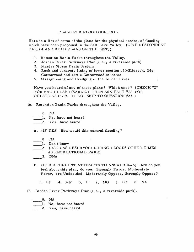
PLANS FOR FLOOD CONTROL

Here is a list of some of the plans for the physical control of flooding which have been proposed in the Salt Lake Valley. (GIVE 'RESPONDENT CARD 4 AND READ PLANS ON THE LIST.)

1. Retention Basin Parks throughout the Valley. 2. Jordan River Parkways Plan (i. e., a riverside park) 3. Master Storm Drain System 4. Rock and concrete lining of lower section of Millcreek, Big

Cottonwood and Little Cottonwood streams. 5. Straightening and Dredging of the Jordan River

Have you heard of any of these plans? Which ones? (CHECK "2" FOR EACH PLAN HEARD OF THEN ASK PART "A" FOR QUESTIONS 15-19. IF NO, SKIP TO QUESTION #23. )

16. Retention Basin Parks throughout the Valley.

o. __ 1.

2.

NA No, have not heard Yes, have heard

A. (IF YES) How would this control flooding?

o. NA 1. Don't know 2. (USED AS RESERVOIR DURING FLOODS OTHER TIMES

AS RECREATIONAL PARK) 3. DNA

B. (IF RESPONDENT ATTEMPTS TO ANSWER l6-A) How do you feel about this plan, do you: Strongly Favor, Moderately Favor, are Undecided, Moderately Oppose, Strongly Oppose?

5. SF 4. MF 3. U 2. MO 1. SO o. NA

17. Jordan River Parkways Plan (i. e., a riverside park).

o. NA 1. No, have not heard

__ 2. Yes, have heard

90

'18. Master Storm. Drain System.

O. NA 1. No, have not heard 2. Yes, ha ve hea rd

A. (IF YES) How would this control flooding?

O. NA 1. Donlt know 2. (SEVERAL UNDERGROUND PIPES LARGE ENOUGH TO

CONTAIN FLOOD WATERS.) 3. DNA

B. (IF RESPONDENT ATTEMPTS TO ANSWER l8-A) How do you feel about this idea, do you:

5. SF 4. MF 3. U 2. MO 1. SO O. NA

19. Rock and concrete lining of lower sections of Millcreek, Big Cottonwood and Little Cottonwood stream.s.

O. NA 1. No, have not heard 2. Yes, have heard

A. (IF YES) How would this control flooding?

O. NA 1. DonI t know 2. (WOULD PREVENT SILTING: ALLOW FOR ENLARGEMENT

OF STREAM CAPACITY.) 3. DNA

B. (IF RESPONDENT ATTEMPTS TO ANSWER 19-A) How do you feel about this idea, do you:

5. SF 4. MF 3. U 2. MO 1. SO

20. Straightening and Dredging of the Jordan River

O. 1. 2.

NA No, have not heard Yes, have heard

91

O. NA

A. (IF YES) How would this control flooding?

O. NA 1. Don't know 2. (ENLARGE THE CHANNEL BY WIDENING AND DEEPENING) 3. DNA

B. (IF RESPONDENT ATTEMPTS TO ANSWER 20-A) How do you feel about this method:

5. SF 4. MF 3. U 2. MO 1. SO O. NA

21. (USE CARD 4) Whi'ch of the following ideas that you have heard of would you prefer to be used if only one plan could be implemented?

O. NA 1. Retention Basin Parks 2. Jordan Parkways 3. Master Storm Drain System 4. Rock and Concrete Channelization of Streams 5. Straightening and Dredging of Streams 6. DNA

A. In your opinion what main feature of this plan makes it desirable?

00. 01. 02. 03. 04. 05. 06. 07.

No Answer Don't know Does not apply Effectiveness in controlling floods Beauty or aesthetic reasons Recreational reasons Naturalness or ecological reasons Economical reasons Other (Specify) __________________ ------__________ __

22. Which of the five plans do you least favor?

1. 2. 3. 4. 5.

Retention Basin Parks Jordan Parkways Master Storm Drain System Rock and Concrete Channelization of streams Straightening and Dredging the Jordan

92

A. In your opinion what main feature of this plan makes it undesirable?

00. No Answer 01. Don't know 02. Does not apply 03. Not effective in controlling floods 04. Not aesthetic or beautiful 05. Lack of recreational features 06. Harmful or does not consider ecological factors 07. Economic co st s too high

Other (Specify) ____________________________________ __

23. Have you attended a meeting or public hearing since 1965 in which flood control projects or problems were the main topic discussed?

O. NA 1. No, 2. Yes, meeting __ 3, Yes, Hearing

(IF YES)

A. How many meeting s did you attend? --------------------------B. What group( s) sponsored the meeting? -----------------------C. When were the meetings held? --------------------------------

24. Has your spouse attended any of these meetings since 1965? O. NA __ 3. Yes, Hearing 1. No, 4. DNA 2. Yes, Meeting

(IF YES)

A. How many meeting s did he (she) attend? ---------------------B. What group( s) sponsored the meetings? ----------------------C. When were the meetings held? --------------------------------25. Since 1965 have you belonged to a citizen group or other organization

that was mainly interested in flood control projects?

O. NA, 1. No 2. Yes, Citizen Group

93

3. Yes, Other Org.

(IF YES)

. A. Which group(s) have you belonged to? ________ _

B. (IF A CITIZEN GROUP) Who are the leaders? -----

26. Has your spouse belonged to a citizen group or other organization related to flood control since 1965?

O. NA __ 3. Yes, Other organization 1. No 4. DNA I

2. Yes, Citizen Group

(IF YES)

A. Which group( s) ------------------------------B. (IF A CITIZEN GROUP) Who are the leaders? ----

27. Have you worked to promote any flood control propo sa1s or ideas since 1965 by petitioning, writing letters, or by other means?

O. NA, __ 1. No, __ 2. Yes

A. (IF YES) Which proposal( s) or idea( s)?

00. ----01. ---02. 03. 04.

05. 06. 07. 08.

__ 09. 10.

NA Retention Basin Parks Jordan Parkways Master Storm Drain System Rock and Concrete Channelization of lower sections of Big and Little Cottonwood and Millcreek Streams. Straightening and Dredging the Jordan River. Watershed Management Flood Plain Zoning Restriction Reservoirs in watershed areas Reservoirs on Jordan River Restrict building on steep slopes Other (Specify) _______________ _

94

B. What did you do?

o. 1. 2.

NA Petition Letter Other (Specify) ________________ _

28. Has your spouse worked to promote any flood control proposals of ideas since 1965 by petitioning, writing letters, or by other means?

__ 0. NA, 1. No, 2. Yes 3. DNA

(IF YES) A. Which proposal( s) or idea( s) ?

00. 01. 02. 03. 04.

05. 06. 07. 08.

__ 09. 10.

No Answer Retention Basin Parks Jordan Parkways Master Storm Drain System Rock and Concrete Channelization of lower sections of Big and Little Cottonwood and Millcreek streams. Straightening and Dredging the Jordan River Watershed Management Flood Plain Zoning restrictions Reservoirs on watershed areas Reservoirs on Jordan River Restrict building on steep slopes Othe r (Specify) ------------------------------------

B. What did he (she) do?

o. 1. 2.

NA Petition Letter Other (Specify) _______________ _

29. Have you opposed any flood control proposals or ideas since 1965 by petitioning, writing letters, vocal protests or other means?

o. NA, 1. No, 2. Yes

(IF YES) A. Which proposal( s) and idea( s)?

95

00. __ Ol.

02. 03. 04.

os. 06. 07. 08.

__ 09. 10.

No Answer Retention Basin Parks Jordan Parkways Master Storm Drain System Rock and Concrete Channelization of lower sections of Big and Little Cottonwood and Millcreek streams. Straightening and Dredging the Jordan River Watershed Management Flood Plain Zoning restrictions Reservoirs in watershed areas Reservoirs on Jordan River Restrict building on steep slopes Other (Specify) ______________________________ ___

B. What did you do?

0. l. 2. 3.

NA Petition Letter Vocal Protest Other (Specify) _______________ __

30. Has your spouse opposed any flood control proposals or ideas since 1965 by petitioning, writing letters, vocal protests or othe r means?

0. NA, 1. No, 2. Yes,

(IF YES) A. Which proposa1( s) or idea{ s) ?

00. Ol. 02. 03. 04.

os. 06. 0.7 .

_08. 09. 10.

No Answer Retention Basin Parks Jordan Parkways Master Storm Drain System Rock and Concrete Channelization of lower sections of Big and Little Cottonwood and Millcreek streams Straightening and Dredging the Jordan River Watershed Management Flood Plain Zoning restrictions Reservoirs in watershed areas Reservoirs in Jordan River Restrict building on steep slopes Other {Specify) _______________ _

96

(1)

(2)

(3)

(4)

(5)

(6)

(7)

(8)

B. What did he (she) do?

O. NA __ 1. Petition

2. Letter Other (Specify) ---------------------------------

31. Do you think it is economically feasible to use the Jordan River as a focal point for developing a recreational park?

O. NA, __ 1. DK, 2. No, 3. Yes

SOCIAL PARTICIPATION

32.

What groups, clubs or organizations do you belong to? (N EED ONLY INFORMATION ON RESPONDENT) We are thinking of organizations such as: Lodges, Civic, Educational, Religious and Neighborhood Groups. (DO NOT INCLUDE PROFESSIONAL GROUPS UNIONS OR ANY NON- VOLUNTARY GROUPS. )

33. 34. 35. No. of yearly What Proportion Reg. What Committees

Name mtgs. Mtgs. Attended in or Offices in of Organization held Past Two Years? Past Two Years?

0 1/4 112 ~JA

97

36. To what extent do you feel that the local citizens have control over what happens in this community?

o. NA 4. Some control l. DK --5. Quite a bit of control 2. Almost no control _6. Almost complete control 3. Very little control

37. Compared to other areas of the same size, would you say that the taxes in Salt Lake County (City) are:

o. NA 4. Moderate -1. DK 5. high 2. very low 6. very high 3. Low

38. (USE CARD 5) Please rate on a scale from 0 to 6 the amount of beauty you associate with each of the particular features we name. o indicates no beauty and 6 extreme beauty. (CODE NA as "7", DK as "8".)

01. A shopping mall 0 I 2 3 4 5 6 02. A natural lake 0 I 2 3 4 5 6 03. Open areas covered 0 I 2 3 4 5 6

large ly with sage 0 I 2 3 4 5 6 04. A natural stream 0 1 2 3 4 5 6 05. A large airport 0 I 2 3 4 5 6 06. A forested mountain canyon 0 1 2 3 4 5 6 07. A city park 0 1 2 3 4 5 6 08. A large cement dam 0 I 2 3 4 5 6 09. A man-made lake or 0 I 2 3 4 5 6

reservoir 10.. Tall skyscrapers 0 I 2 3 4 5 6 II. Terraced hillsides 0 I 2 3 4 5 6 12. An earth dam 0 I 2 3 4 5 6 13. A trimmed and planted yard 0 I 2 3 4 5 6 14. A view of fields and farms 0 I 2 3 4 5 6

RECREATION

3 9. Do you feel that the number of public parks in Salt Lake City and County (not including mountain canyons) is adequate or not adequate?

O. NA, 1. DK, 2. Not adequate, 3. Adequate

98

4 O. (USE CARD 9) To what degree would you say your yard is a source of pleasure to you?

No Pleasure

o I 2 3 4

Great Pleasure NA

567 DK 8

4 1. (IF RESPONDENT LIVES ON A STREAM) To what degree would you say the stream in your backyard is a source of pleasure to you? (USE CARD 9)

No Pleasure

o I 2 3 4

ATTITUDES TOWARD LEISURE ACTIVI1Y

Great Pleasure NA

567 DK 8

(USE CARD 2) The next few statements express different ways a person may f eel about a leisure activity. Please select the answer which best descr ibes the way you feel about each: Strongly Agree, Agree, Undecided, Disagree, or Strongly Disagree.

42. Frankly speaking, much of the time work is pretty dull, but leisure makes life worthwhile.

5. SA 4. A 3. U 2. D /1. SD O. NA

43. I generally feel guilty when I enjoy leisure for more than a short time.

1. SA 2. A 3. U 4. D 5. SD O. NA

44. Today most people spend too much time just enjoying themsleves.

1. SA 2. A 3. U 4. D 5. SD O. NA

45. I sometimes feel guiJty when I'm on vacation because I'm not working.

1. SA 2. A 3. U 4. D 5. SD O. N A

46. I generally get more enjoyment out of leisure activities than I do out of work activities.

5. SA 4. A 3. U 2. D 1. SD O. N A

99

47. Generally speaking the main satisfaction I get out of life is working.

1. SA 2. A 3. U 4. D 5. SD o. N A

TOTAL LEISURE ORIENTATION SCORE

ATTITUDES TOWARD ENVrnONMENTAL FACTORS

(USE CARD 2) Now I would like to know how you feel about some statements regarding the environment.

48. Whatever the financial costs, the Jordan River should be c.leaned up so that fishing and swimming in the River would be safe.

5. SA 4. A 3. U 2. D 1. SD o. N A

49. The so called evils of water pollution are greatly exaggerated by many people.

1. SA 2. A 3. U 4. D 5. SD o. N A

50. People should not be allowed to build homes next to stream~ if they contribute to the pollution.

5. SA 4. A 3. U 2. D 1. SD o. N A

51. Economic development is of first importance and therefore no resource should be restricted from economic use.

1. SA 2. A 3. U 4. D 5. SD o. N A

52. The ill effects of pesticides on the environment cannot be emphasized too much.

5. SA 4. A 3. U 2. D 1. SD o. NA

53. People should not be allowed to build homes next to streams because they often destroy the beauty of the stream.

5. SA 4. A 3. U 2. D 1. SD o. NA

54. Official wilderness areas that are set aside for permanent ~reservation should prohibit all future use or development of any kind such as minerals and water resources.

5. SA 4. A 3. U 2. D 1. SD o. NA

100

---

55. Not enough emphasis is being placed on the beautification and improvement of areas around large constructed reservoirs.

5. SA 4. A 3. U 2. D 1. SD o. N A

56. Our natural environment has deteriorated to a great extent in the last few years.

5. SA 4. A 3. U 2. D 1. SD O. NA

57. The inf ormation value of highway advertising billboards is more important than the unattractiveness they made on our landscape.

1. SA 2. A 3. U 4. D 5. SD O. N A

TOTAL ENVIRONMENTAL ORIENTATION SCORE ---58. (USE CARD 10) Suppose it were found that an industry were responsible

for significant pollution to a stream or lake. What action should be taken?

O. NA 1. DK 2. No outside action should be taken, the industry should be allowed

to continue as is. 3. The polluter should be notified, but corrective action should be

voluntary with government financial assistance available. 4. The polluter should be notified, but corrective action should

be voluntary al d at his own expense. 5. The polluter should be required by law to stop the pollution but

the government should provide financial assistance. 6. The polluter should be required by law to stop the pollution at

his own expenses.

5 9. (USE CARD 11) Suppose dairy farmers could significantly reduce pollution caused by manure spreading by improved storage practices. How much more would you be willing to pay for a half-gallon of milk if it would allow them to adopt these practices?

O. NA 4. Up to 5<; 1. DK 5. Up to 10<; 2. None 6. More than 10<; 3. Up to 2<; a half gallon 7. Whatever it costs

101

60. A number of government agencies have been established to regulate and monitor different forms of air, water and land pollution. ' In general, how strict do you feel the standards set by these agencies are?

0. NA 4. About right --1. DK 5. Too lenient --2. Much too strict 6. Much too lenient 3. Too strict

61. Can you think of the names of any governmental agencies whose ~ purpose in Salt Lake Gity and County is flood control?

A.

B. o. NA 1. DK 2. Respondent did ~ mention either the Corps of Engineers

or the Salt Lake Couno/ Flood Control Department. 3. Respondent mentioned the Corps of Engineers but not the

Salt Lake County Flood Control Department. 4. Respondent mentioned the Salt Lake County Flood Control

Department but not the Corps of Engineers. 5. Respondent mentioned both the Corps of Engineers and the

Sat Lake County Flood Control Department.

POLITICAL AND SOCIAL QUESTIONS

For comparative purposes, your opinions on other things will also be of value to us. We now have a few questions on political activity and other factors.

62. In the last four years have you written or talked to your congressman or any other public official to let them know what you would like them to do on a public issue you are interested in?

__ 0. No, __ 1. Yes, 2. N A

63. In the last four years have you worked for the election of any political candidate by doing things like distributing circulars or leaflets, making speeches, or calling on voters?

0. No, ' 1. Yes, __ 2. NA

102

64. In the last four years have you contributed money to a political part or to a candidate for a political office?

__ 0. No, 1. Yes 2. NA

65. Have you voted in ei ther of the last 2 elections? (Includes elections at the loc al leve 1)

0. No, 1. Yes, 2. NA

TOTAL SCORE OF ITEMS 62-63 ----Please listen carefully to the following statements and tell me how you feel. On these just indicate whether you agree or disagree.

66. There is no way other than voting that people like me can influence actions of the government.

__ 0. Agree, __ 1. Disagree, __ 2. NA, 3. DK

67. Sometimes politics and government seem so complicated that I can't really understan d what's going on.

__ 0. Agree, __ 1. Disagree, __ 2. NA, 3. DK

68. People like me don't have any say about what the government does.

__ 0. Agree, __ 1. Disagree, __ 2. NA, 3. DK

69. I believe public' officials don't care much what people like me think.

0. Agree, 1. Disagree, __ 2. NA, 3. DK

TOTAL SCORE OF ITEMS 66-69 ----

FAMILY BACKGROUND INFORMA TION

Finally for statistical purposes we would like to ask these questions about you and your family.

70. Where were you born? ----------------------VILLAGE, TOWN, CITY STATE OR COUNTRY

103

71. (USE CARD 12) Which of the following best describes the types of area in which you mainly lived between the ages of 1 and 18.

00. NA Ol. DK --02. Open Country 03. Small town, less than 10, 000 04. Town or city, 10, 000 to 50, 000 05. Large city over 50, 000 06. (02 and 03 equally) 07. (02 and 04 equally) 08. (02 and 05 equally) 09. (02 and 03, and 04 equally) 10. (all four areas equally) II. (03 and 04 equally) 12. (03 and 05 equally) 13. (03 and 04 and 05 equally) 14. (04 and 05 equally)

72. Approximately how long have you lived in your present home?

00. NA 09. 31-35 years --OI. Less than one year 10. 36-40 years 02. 1 to 3 years II. 41-45 years --03. 4-5 years 12. 46-50 years 04. 6-10 years 13. 51-55 years -- --05. 11-15 years 14. 56-60years --06. 16-20 years 15. 61-65 years 07. 21-25 years 16. over 65 years --08. 26-30 years

73. How long have you lived anywhere in Salt Lake County (including Salt Lake City)?

00. NA 09. 31-35 years --OI. Less than one year 10. 36-40 years 02. 1 to 3 years 11. 41-45 years 03. 4-5 years 12. 46~50 years 04. 6-10 years 13. 51-55 years 05. 11-15 years -- 14. 56-60 years 06. 16-20 years 15. 61-65 years 07. 21-25 years 16. over 65 years 08. 26-30 years

104

74. Would you mind giving me the year of your birth? (CODE ONLY LAST TWO DIGITS OF ACTUAL NUMBER GIVEN, CODE DK AND NA AS "73") ---

7 5. Present marital status.

o. NA 1. Separated or divorced 2. Widowed 3. Never Married 4. Married

76. What was the last grade of school you and your spouse completed? Male: Female:

A. Husband or Male Head

O. NA 1. Graduate Degree

(MA, MS, ME, MD, Ph. D., LLD) 2. 4 year college graduate 3. 1-3 years college 4. Business or trade school 5. High school graduate 6. 10-11 years of school 7. 7 .... 9 years of school 8. Les s than 7 years 9. DNA

7 7. How many children do you have?

o. None 1. One 2. Two 3. Three --4. Four

B. Wife or Female Head

o. NA 1. Graduate Degree

(MA, MS, ME, MD, Ph.D., LLD)

2. 4 years college graduate 3. 1-3 years college 4. Business or trade school

High school graduate 10-11 years of school

5. - 6. 7. 7 -9 years of school 8. Less than 7 years 9. DNA

5. Five 6. Six 7. Seven or more 8. NA 9. DNA (includes never married,)

A. (IF CHILDREN) How many of these live at home at least 8 months of the year? (USE SAME CODE AS #85) ___________ _

B. (IF CHILDREN) How many of these are under 6 years of age? (USE SAME CODE AS #85) ______________ _

105

78. What kind of work do you and your spouse do?

A. Husband's or Male Head's Major Occupation

(1) Job Title ----------------------------------------(2) Brief Description ------------------------------(3) Industry ______________________________ _

(4) (IF EXECUTIVE MANAGER OR OWNER OF A BUSINESS) Which of the following figures comes closest to the value of the business? (USE CARD 13)

1. Less than $3, 000 4. Between $35, 000-$100, 000 2. Between $3,000-$6,000 5. Between $100, 000-$500, 000 I

3. Between $6, 000-$35, 000 6. Over $500, 000

B. Husband's or Male Head's Part-Time Occupation

(1) Job Title ---------------------------------------(2) Brief De scri ption_--___________________________ _ (3) Industry -----------------------------------------(4) Value of Business (LIST CODE NUMBER IN 86-A-(4) IF APPLICABLE __

C. Wife's or Female Head's Major Occupation

(1) Job Title ---------------------------------------(2) Brief Description --------------------------------(3) Industry _____________________________ _

(4) Value of Business (LIST CODE NUMBER IN 86-A-(4) IF APPLICABLE __

D. Wife's of Female Head's Part-Time Occupation

(1) Job Title ____________________ _ ('2) Brief Description~ ___________________________ _ (3) Industry _________________________________ _

(4) Value of business (LIST CODE NUMBER IN 86-A-(4) IF APPLICABLE __

79. Are you buying or renting your home?

____ 0. NA, __ 1. Renting, __ 2. Buy or own

8 O. (USE CARD 14) Taking into consideration all sources of income for you and your spouse which category on this card represents your total income before your taxes in 1971?

106

o. NA or DK 5. $9, 000-$11, 999 --1. Under $3, 000 6. $12,000-$14, 999 --2. $3,000-$4,999 7. $15,000-$19,999 3. $5,000-$6,999 --8. $20,000-$24,999 4. $7,000-$8,999 9. $25,000 and over --

8 1. Are there any other ideas or comments that you would like to make . concerning anything we have discussed ? __________ _

QUESTIONS FOR INTERVIEWER ONLY)

82. Sex of respondent: __ 1. Male, 2. Female

83. Type of structure in which family lives:

1. trailer or mobile home 2. Detached single family home 3. 2 to 3 fam ily apartme nt house or row 4. detached 2 to 4 family house (apartments in old house) 5. row house (4 or more units in an attached row) 6. apartment house (4 or more units) 7. apartment in partly commercial structure 8. other(speci~) ________________________________ _

84. Describe conditions of respondent's home, yard and neighborhood

A. Overa 11

B. Lawns

C. f10we

D. Shade menta

E. house

F. house

r

1

gardens

and Orna-trees

exterior

interior

G. neigh ratin

borhood g

O. has

none

1. 2. 3. 4. poor good or

or low fair average above ave.

_._---

107

5. very good

,or high

r---

_.

--~--

85. Thumbnail Sketch: Anything else about the respondent, the interview situation, the house, or the neighborhood that seems important? Some factors to consider are interest, apparent intelligence, suspicions, others present, in a hurry or not etc. ______________ _

86. Other notes: _________________________ _

108