A performance comparison of Clojure and Java - DiVA portal

IN DEGREE PROJECT COMPUTER SCIENCE AND ENGINEERING,SECOND CYCLE, 30 CREDITS

, STOCKHOLM SWEDEN 2019

A performance comparison of Clojure and Java

GUSTAV KRANTZ

KTH ROYAL INSTITUTE OF TECHNOLOGYSCHOOL OF ELECTRICAL ENGINEERING AND COMPUTER SCIENCE

A performance comparison ofClojure and Java

GUSTAV KRANTZ

Master in Computer ScienceDate: December 25, 2019Supervisor: Håkan LaneExaminer: Elena TroubitsynaSchool of Electrical Engineering and Computer ScienceSwedish title: En prestandajämförelse för Clojure och Java

iii

AbstractClojure is a relatively new functional programming language that can com-pile to both Java bytecode and JavaScript(ClojureScript), with features likepersistent data structures and a high level of abstraction.

With new languages it is important to not only look at their features, butalso evaluate how well they perform in practice. Using methods proposed byGeorges, Buytaert, and Eeckhout [1], this study attempts to give the reader anidea of what kind of performance a programmer can expect when they chooseto program in Clojure. This is done by first comparing the steady-state runtimeof Clojure with that of Java in several small example programs, and then com-paring the startup time of Clojure with that of Java using the same exampleprograms.

It was found that Clojure ran several times slower than Java in all conductedexperiments. The steady-state experiments showed that the slowdown factorsranged between 2.4826 and 28.8577. The startup slowdown factors observedranged between 2.4872 and 52.0417.

These results strongly suggest that the use of Clojure over Java comes witha cost of both startup and runtime performance.

iv

SammanfattningClojure är ett relativt nytt funktionellt programmeringsspråk som kan kompi-lera till både Java bytecode och JavaScript(ClojureScript), med funktionalitetsom persistenta datastrukturer och en hög abstraktionsnivå.

Med nya språk är det viktigt att inte bara kolla på dess funktionalitet, utanockså utvärdera hur dom presterar i praktiken. Genom att använda metodersom föreslogs av Georges, Buytaert och Eeckhout [1], så har den här studienförsökt ge läsaren en uppfattning av vilken sorts prestanda man kan förväntasig när man väljer att programmera i Clojure. Detta gjordes genom att förstjämföra steady-state-prestandaskillnaden mellan Clojure och Java i ett flertalsmå exempelprogram, och sen jämföra starttiden mellan de två programme-ringsspråken i samma exempelprogram.

Man kom fram till att Clojure körde flera gånger segare än Java i alla ge-nomförda experiment, för både steady-state- och starttidsexperimenten. Steady-state-experimenten visade nedsegningsfaktorer mellan 2.4826 och 28.8577.Starttidsexperimenten visade nedsegningsfaktorer mellan 2.4872 och 52.0417.

Dessa resultat pekar på att användning av Clojure kommer med en prestan-dakostnad för både starttid och körtid.

Contents

1 Introduction 11.1 Research questions . . . . . . . . . . . . . . . . . . . . . . . 21.2 Hypothesis . . . . . . . . . . . . . . . . . . . . . . . . . . . 2

2 Background 32.1 Java and Clojure . . . . . . . . . . . . . . . . . . . . . . . . . 3

2.1.1 Java . . . . . . . . . . . . . . . . . . . . . . . . . . . 32.1.2 Clojure . . . . . . . . . . . . . . . . . . . . . . . . . 32.1.3 Immutability . . . . . . . . . . . . . . . . . . . . . . 32.1.4 Concurrency . . . . . . . . . . . . . . . . . . . . . . 52.1.5 Types . . . . . . . . . . . . . . . . . . . . . . . . . . 52.1.6 Motivation for Clojure . . . . . . . . . . . . . . . . . 6

2.2 The Java virtual machine . . . . . . . . . . . . . . . . . . . . 62.2.1 Just-in-time compilation . . . . . . . . . . . . . . . . 62.2.2 Garbage collection . . . . . . . . . . . . . . . . . . . 72.2.3 Class loading . . . . . . . . . . . . . . . . . . . . . . 7

2.3 Steady-state . . . . . . . . . . . . . . . . . . . . . . . . . . . 72.4 Leiningen . . . . . . . . . . . . . . . . . . . . . . . . . . . . 102.5 Previous research . . . . . . . . . . . . . . . . . . . . . . . . 10

2.5.1 Quantifying performance changeswith effect size con-fidence intervals . . . . . . . . . . . . . . . . . . . . 10

2.5.2 Statistically rigorous Java performance evaluation . . . 112.6 Runtime inconsistencies . . . . . . . . . . . . . . . . . . . . 11

2.6.1 Startup times . . . . . . . . . . . . . . . . . . . . . . 112.7 Practical clojure . . . . . . . . . . . . . . . . . . . . . . . . . 11

2.7.1 Type hinting . . . . . . . . . . . . . . . . . . . . . . 122.7.2 Primitives . . . . . . . . . . . . . . . . . . . . . . . . 122.7.3 Dealing with persistence . . . . . . . . . . . . . . . . 132.7.4 Function inlining . . . . . . . . . . . . . . . . . . . . 13

v

vi CONTENTS

3 Method 153.1 Sample programs . . . . . . . . . . . . . . . . . . . . . . . . 15

3.1.1 Recursion . . . . . . . . . . . . . . . . . . . . . . . . 163.1.2 Sorting . . . . . . . . . . . . . . . . . . . . . . . . . 163.1.3 Map creation . . . . . . . . . . . . . . . . . . . . . . 163.1.4 Object creation . . . . . . . . . . . . . . . . . . . . . 173.1.5 Binary tree DFS . . . . . . . . . . . . . . . . . . . . 173.1.6 Binary tree BFS . . . . . . . . . . . . . . . . . . . . 17

3.2 Steady-state experiments . . . . . . . . . . . . . . . . . . . . 183.2.1 Measurement method . . . . . . . . . . . . . . . . . . 183.2.2 Data gathering . . . . . . . . . . . . . . . . . . . . . 183.2.3 Confidence interval calculation . . . . . . . . . . . . . 18

3.3 Startup time experiments . . . . . . . . . . . . . . . . . . . . 193.3.1 Measurement method . . . . . . . . . . . . . . . . . . 193.3.2 Data gathering . . . . . . . . . . . . . . . . . . . . . 20

3.4 System specifications . . . . . . . . . . . . . . . . . . . . . . 203.4.1 Software . . . . . . . . . . . . . . . . . . . . . . . . 20

4 Results 214.1 Steady-state results . . . . . . . . . . . . . . . . . . . . . . . 21

4.1.1 Recursion . . . . . . . . . . . . . . . . . . . . . . . . 224.1.2 Sorting . . . . . . . . . . . . . . . . . . . . . . . . . 234.1.3 Map creation . . . . . . . . . . . . . . . . . . . . . . 244.1.4 Object creation . . . . . . . . . . . . . . . . . . . . . 254.1.5 Binary tree DFS . . . . . . . . . . . . . . . . . . . . 264.1.6 Binary tree BFS . . . . . . . . . . . . . . . . . . . . 27

4.2 Startup time results . . . . . . . . . . . . . . . . . . . . . . . 284.2.1 Recursion . . . . . . . . . . . . . . . . . . . . . . . . 294.2.2 Sorting . . . . . . . . . . . . . . . . . . . . . . . . . 304.2.3 Map creation . . . . . . . . . . . . . . . . . . . . . . 314.2.4 Object creation . . . . . . . . . . . . . . . . . . . . . 324.2.5 Binary tree DFS . . . . . . . . . . . . . . . . . . . . 334.2.6 Binary tree BFS . . . . . . . . . . . . . . . . . . . . 34

5 Discussion 355.1 Steady-state results . . . . . . . . . . . . . . . . . . . . . . . 35

5.1.1 Irregularities . . . . . . . . . . . . . . . . . . . . . . 355.2 Startup time results . . . . . . . . . . . . . . . . . . . . . . . 35

5.2.1 Irregularities . . . . . . . . . . . . . . . . . . . . . . 36

CONTENTS vii

5.3 Threats to validity . . . . . . . . . . . . . . . . . . . . . . . . 365.3.1 Unfair testing environment . . . . . . . . . . . . . . . 365.3.2 Non-optimal code . . . . . . . . . . . . . . . . . . . . 36

5.4 Future work . . . . . . . . . . . . . . . . . . . . . . . . . . . 365.5 Sustainability & social impact . . . . . . . . . . . . . . . . . 375.6 Method selection - Sample programs . . . . . . . . . . . . . . 37

6 Conclusion 38

Bibliography 39

A Experiment code 42A.1 Recursion . . . . . . . . . . . . . . . . . . . . . . . . . . . . 42A.2 Sorting . . . . . . . . . . . . . . . . . . . . . . . . . . . . . 43A.3 Map creation . . . . . . . . . . . . . . . . . . . . . . . . . . 44A.4 Object creation . . . . . . . . . . . . . . . . . . . . . . . . . 44A.5 Binary Tree DFS . . . . . . . . . . . . . . . . . . . . . . . . 45A.6 Binary Tree BFS . . . . . . . . . . . . . . . . . . . . . . . . 46

Chapter 1

Introduction

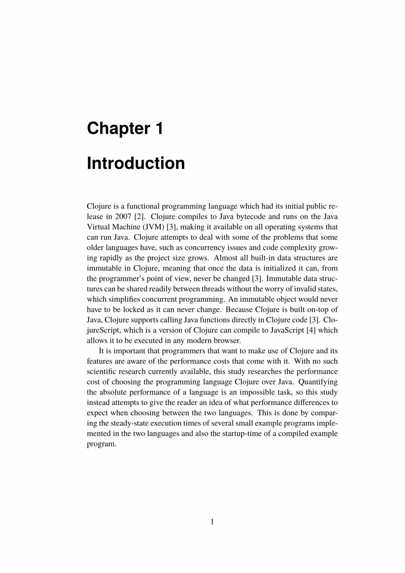
Clojure is a functional programming language which had its initial public re-lease in 2007 [2]. Clojure compiles to Java bytecode and runs on the JavaVirtual Machine (JVM) [3], making it available on all operating systems thatcan run Java. Clojure attempts to deal with some of the problems that someolder languages have, such as concurrency issues and code complexity grow-ing rapidly as the project size grows. Almost all built-in data structures areimmutable in Clojure, meaning that once the data is initialized it can, fromthe programmer’s point of view, never be changed [3]. Immutable data struc-tures can be shared readily between threads without the worry of invalid states,which simplifies concurrent programming. An immutable object would neverhave to be locked as it can never change. Because Clojure is built on-top ofJava, Clojure supports calling Java functions directly in Clojure code [3]. Clo-jureScript, which is a version of Clojure can compile to JavaScript [4] whichallows it to be executed in any modern browser.

It is important that programmers that want to make use of Clojure and itsfeatures are aware of the performance costs that come with it. With no suchscientific research currently available, this study researches the performancecost of choosing the programming language Clojure over Java. Quantifyingthe absolute performance of a language is an impossible task, so this studyinstead attempts to give the reader an idea of what performance differences toexpect when choosing between the two languages. This is done by compar-ing the steady-state execution times of several small example programs imple-mented in the two languages and also the startup-time of a compiled exampleprogram.

1

2 CHAPTER 1. INTRODUCTION

1.1 Research questionsHow does Clojure measure up against Java in terms of execution speed?How does Clojure measure up against Java in terms of startup-time?

1.2 HypothesisThe first hypothesis is that the steady-state execution speed of Clojure will besignificantly slower than Java in most experiments. (But could get close insome cases as they both compile to Java bytecode and run on the same virtualmachine.) The second hypothesis is that the startup-time will be several ordersof magnitude slower for Clojure than that of Java.

Chapter 2

Background

2.1 Java and Clojure

2.1.1 JavaJava is a typed object-oriented language with a syntax derived from C whichwas released by Oracle in January 1996 (version 1.0) along with the Java Vir-tual Machine or JVM [5]. According to the TIOBE Index [6] Java is the mostpopular programming language as of June 2019 and has been for the majorityof the time since 2002. Having the advantage of being so popular, and beingbacked by a multi billion dollar company, Java and the JVM has since 1996been updated and optimized many times [7].

2.1.2 ClojureClojure is a dynamically typed functional language with a Lisp syntax whichhad its first public release in 2007 [2, 8]. Clojure is according to the TIOBEIndex [6] the 48th most popular programming language as of June 2019. WithClojure being a younger language and much less popular, it has received fewerupdates [2] and is likely much less optimized than other languages. However,as it compiles to Java bytecode, it can make use of the JVM that Oracle hasoptimized for more than two decades and take advantage of the optimizationtechniques that it uses, some of which are mentioned in 2.2.

2.1.3 ImmutabilityClojure’s built-in data structures are immutable, which means that once ini-tialized, they cannot change. As an example, adding the integer 3 to a list

3

4 CHAPTER 2. BACKGROUND

containing the integers 1 and 2 in Clojure will result in two lists, namely thelist prior to the operation (1, 2) and the list after the operation (1, 2, 3). In Java,adding to a list will modify it and after the operation only one list will exist.

This system might sound very slow and memory intensive at first as onemight think that new memory would have to be allocated and the data fromthe first list would have to be copied to create the new list. However, sincethe data is immutable, we can use clever techniques to share the data betweendifferent instances of data structures. Figure 2.1 shows how memory sharingis possible for three immutable lists resulting from the following operations:

1. Define List a as (1, 2)

2. Add 3 to List a and save it as List b

3. Drop one item from List b and save it as List c

Figure 2.1: An example of how memory sharing between immutable lists sup-porting adding-to-tail and dropping-from-head is possible. The squares repre-sent Java objects. This example is not taken from any programming language.

This approach would result in constant time and space complexity for bothadding one item and dropping one item, whereas the unoptimized copyingapproach would result in linear complexities relative to the length of the lists.

Clojure makes use of similar, but more complex approaches to reduce thetime and space complexity of functions that manipulate its immutable datastructures [9].

There are however exceptions to the immutability of Clojure’s data struc-tures. For example, atoms are mutable and are designed to hold an immutabledata structure to be shared with other threads [10].

CHAPTER 2. BACKGROUND 5

2.1.4 ConcurrencyClojure was designed with concurrency in mind. On the Clojure website 1 itis claimed that mutable stateful objects are the new "spaghetti code" and thatthey lead to a concurrency disaster. Immutability removes the need for lockswhen programming concurrent code as the data can only be read and can notbe changed. Furthermore, Clojure has abstracted away the need of locks evenwhen writing to a mutable atom using its software transactional memory andagent systems [8]. The syntax for concurrency in Clojure is more compact andarguably simpler than that of Java. Figure 2.2 and 2.3 demonstrate how newthreads can be started in the two languages, but there are of course many otherways to do so.

( f u t u r e ( do t imes [ i 10] ( p r i n t l n i ) ) )

Figure 2.2: Clojure code that starts a new thread that prints the numbers 0 to9.

new Thread ( ){

p u b l i c vo id run ( ) {f o r ( i n t i = 0 ; i < 10 ; ++ i ){

System . ou t . p r i n t l n ( i ) ;}

}} . s t a r t ( ) ;

Figure 2.3: Java code that starts a new thread that prints the numbers 0 to 9.

2.1.5 TypesTheClojure code compiled to Java bytecode that runs on the JVMmakes use ofJava classes. However, this usage is abstracted away from the user and from theprogrammers point of view the data structures are dynamically typed. Whencalling Java functions adding type hints is optional which can help to avoidreflection as discussed in 2.7.1.

1https://www.clojure.org/


2.1.6 Motivation for ClojureThe reason that this work was conducted even though there was a strong ex-pectation that Clojure would perform worse than Java was to confirm or refutesaid expectations using scientific methods, giving the reader a scientific sourceto use when arguing for which language is better for their use case. A resultwhere Clojure performed close to or better than Java would be useful for peo-ple who prefer Clojure due to its functional approach, high abstraction level,ease of multi-threading or personal preference, but who chose Java due to thealleged performance problems. Since there were no previous scientific worksfound that had done this kind of comparison before, this work will also givea scientific ground for future scientific papers that touch on Clojure’s perfor-mance.

2.2 The Java virtual machineThe Java virtual machine or JVM is a virtual machine which, like a real com-puting machine, has a set of instructions, or bytecodes which it can execute.As the JVM executes Java bytecode, and not Java, any language that can tojava bytecode, like Clojure, can execute on the JVM [11].

The execution on the JVM is non-deterministic. This means that executionof the same code on the JVM can have different total runtimes. compile Thisis not only due to the non-determinism of modern computer systems, but alsoJust-in-time compilation, real-time garbage collection and class loading thatall are run on the JVM [12].

Changing settings such as object layout, garbage collection algorithm andheap order on the JVM can have significant effects on the performance of aprogram [1, 13].

2.2.1 Just-in-time compilationA Just-in-time compiler compiles Java bytecode to native machine languagefor faster execution. This is done during runtime, which can affect the totalruntime of a program by both requiring processing power to run the compila-tion and by offering faster execution once finished.


2.2.2 Garbage collectionGarbage collection is the automatic freeing of memory that the JVM offers.As it runs non-deterministically at runtime, it can affect the total runtime of aprogram by interrupting execution.

2.2.3 Class loadingClass loading happens when a class is referenced for the first time. As theloading takes processing power, it can interrupt execution and affect the totalruntime of a program.

2.3 Steady-stateSteady-state exectution refers to the state of the execution of a program whenit is executing at full speed, or when the warm up of the program has finished.This is when things such as class loading (2.2.3) and just-in-time compilation(2.2.1) that run during the start of a program execution have finished and willno longer require processing power. Steady-state execution can be reachedand measured by repeatedly running an experiment until the variance in exe-cution times is under a set threshold. This is possible due to the fact that theruntimes of programs running on the JVM suffer more from variance duringwarm up. It is important to note that even though the post warm up state iscalled ”steady-state”, it still suffers from variance due to the non-deterministicnature of modern computer systems as mentioned in (2.2). Figure 2.4 showsan example of how warm up can affect the runtimes of an experiment. In thatexample the first three executions are strongly affected by warm up and shouldbe discarded when steady-state executions are of interest.


0 10 20 30 40 50 60 70 80 90 100

run index

0.045

0.05

0.055

0.06

0.065

0.07

0.075

0.08

run

tim

e(m

s)

warm up visualization

Figure 2.4: A visualization of how warm up can affect the runtimes of anexperiment. The runtimes were gathered in the order of their index withoutany restart of the virtual machine or the process running the experiment.

Figure 2.5 and 2.6 show how steady-state execution runtimes can be col-lected for an experiment in Java. The example shown collects 30 steady-stateruntimes and considers steady-state to be achievedwhen the coefficient of vari-ation is below 0.025.

Ar r ayL i s t <Double > t ime s = new Ar r ayL i s t <Double > ( ) ;wh i l e ( t r u e ){

doub l e t ime = runExpe r imen t ( ) ;t ime s . add ( t ime ) ;i f ( t ime s . s i z e ( ) > 30){

I t e r a b l e <Double > s u bL i s t = t ime s . s u bL i s t (t ime s . s i z e ( ) − 30 , t ime s . s i z e ( ) ) ;

i f ( cov ( s u bL i s t ) < 0 . 0 2 5 )r e t u r n s u bL i s t ;

}}

Figure 2.5: Java code that collects 30 steady-state runtimes for an experimentusing the function from figure 2.6 to calculate the coefficient of variation.

p r i v a t e doub l e cov ( I t e r a b l e <Double > t ime s ){

doub l e mean = 0 ;i n t coun t = 0 ;f o r ( doub l e d : t ime s ){

mean += d ;coun t ++;

}mean /= coun t ;

doub l e powsum = 0 ;f o r ( doub l e d : t ime s )

powsum += Math . pow ( d − mean , 2 ) ;

doub l e sD e v i a t i o n =Math . s q r t ( powsum / ( count −1 ) ) ;

r e t u r n sD e v i a t i o n / mean ;}

Figure 2.6: A Java function that calculates the coefficient of variation.


2.4 LeiningenLeiningen is a project manager for Clojure which can be used to compile Clo-jure code into .jar (Java archive) files, among other things [14].

2.5 Previous researchThere were no similar scientific works found where Clojure’s performance hadbeen measured and compared to that of other languages. In order to formu-late a hypothesis, other sources were used to see how people have found thatClojure performs in relation to Java. Surveying the web [15, 16, 17, 18, 19]leads one to believe that Clojure is overall slower than Java. The main problempeople seemed to have was that the startup time of Clojure is extremely slowcompared to other languages. VanderHart and Sierra [20] say in their book,which is mentioned more later (2.7), that

In principle, Clojure can be just as fast as Java: both are compiledto Java bytecode instructions, which are executed by a Java VirtualMachine ... Clojure code will generally run slower than equiva-lent Java code. However, with some minor adjustments, Clojureperformance can usually be brought near Java performance. Don’tforget that Java is always available as a fallback for performance-critical sections of code.

2.5.1 Quantifying performance changeswith effect sizeconfidence intervals

Kalibera and Jones [21] conducted a literature study of 122 papers posted atComputer Science conferences and in journals. They found that the Com-puter Science field lacks rigour when it comes to papers that do these kindof performance measurements. Rigour that they say is expected in other ex-perimental sciences. Of the papers that evaluated execution time, about 79%failed to whatsoever mention the uncertainty of the execution times stemmingfrom the non-determinism of our modern day computers. And some onlyincluded the uncertainty of one of the execution times (before and after theperformance changes) when calculating their confidence interval. They alsofound that some papers did not mention how many times they ran their bench-marks, which is worrying as performance of today’s computer systems are


rarely deterministic and can vary from run to run. These mistakes severelyhurt the reliability and reproducibility of the results.

2.5.2 Statistically rigorous Java performance evalua-tion

Another literature study was conducted by Georges, Buytaert, and Eeckhout[1] where they examined 50 papers. Their study, similar to Kalibera and Jones[21], shows that there is a lack of rigour in our field. 16 of the 50 papers evenfailed to state their method of measuring performance, and in the remaining34 they found that the data-analysis part was often disappointing, again, dueto ignorance of the non-determinism of the experiment runtimes. In the samepaper, they also proposed more rigorous methods for calculating performancechanges for Java. This source is mentioned more later as two of their methodsare used to gather experimental data and analyze the data gathered.

2.6 Runtime inconsistenciesRepeatedly running and measuring the execution time of almost any programwill yield a range of runtimes rather than the same runtime being measuredevery time. This is due to non-deterministic factors such asmemory placement[21], scheduling and the startup times mentioned in the next section (2.6.1).To deal with this non-determinism, we can run the experiments multiple timesand calculate a confidence interval.

2.6.1 Startup timesIt has been observed that the JVM has a startup period, where runtimes arelikely to be bigger. This is most likely due to class loading and Just-In-Timecompilation. To deal with this you can repeatedly run your experiments, waituntil the startup period has passed and the runtimes have stabilized, only thendo you start saving the runtime data for your data analysis [1] as mentioned in(2.3).

2.7 Practical clojureVanderHart and Sierra [20] argue that Clojure runs slower than Java but thatoptimized Clojure can be brought to near Java performance. With that claim


they also presented some optimization techniques, some of which will be men-tioned following.

2.7.1 Type hintingAs Clojure is not statically typed, it does not always know the types of objectsat runtime. To be able to call Java functions on objects, Clojure uses a Javamethod called reflection which allows calling functions by name. Reflectioncalls are slower than compiled calls, so we can optimize our Clojure code byhinting what type the object of the method we are calling has when we wantto call a function. In some cases we also have to type hint the parameters ofthe function calls and/or the return type.

( de fn nth−cha r [ s n ] ( . cha rA t s n ) )

Figure 2.7: Code that defines a Clojure function that gets the n-th characterin a string by using the Java function charAt. This code will need a reflectivecall as the type of s is not known at runtime [20].

( de fn nth−cha r [#^ S t r i n g s n ] ( . cha rA t s n ) )

Figure 2.8: The same code as above where s is type hinted. This will avoid areflective call [20].

Knowing when to type hint can be difficult, but turning on the flag *warn-on-reflection* will let us know at runtime when we can optimize our code byalerting us when a reflective call is made.

2.7.2 PrimitivesIn Clojure, numbers are Java objects and not primitives, which canmakemath-intensive functions slower. To get around this problem we can coerce our pa-rameters into primitives.

The following code has been observed to be 12 times faster than the samecode without primitives [20].


( de fn gcd [ a b ]( l oop [ a ( i n t a ) , b ( i n t b ) ]

( cond ( z e r o ? a ) b( z e r o ? b ) a( > a b ) ( r e c u r (− a b ) b ): e l s e ( r e c u r a (− b a ) ) ) ) )

Figure 2.9: Clojure code to calculate the greatest common divisor for twointegers. On row 2 the input integers are coerced into primitives [20].

Arrays can also be type-hinted to coerce the elements into primitives.

2.7.3 Dealing with persistenceClojure’s built-in data structures are persistent, meaning that a version of thedata structure will persist when something is added or removed from it. Thismakes building large data structures step-by-step slow. If we are working on asingle thread, we can make the building of data structures transient, meaningwe can add to the data structure without having it persist, and when we arefinished building we can return a persistent version of the data structure.

( l oop [m ( t r a n s i e n t { } ) , i 0 ]( i f ( > i 127)

( p e r s i s t e n t ! m)( r e c u r ( a s s o c ! m ( cha r i ) i ) ( i n c i ) ) ) )

Figure 2.10: Clojure code that shows the use of a transient map [20].

2.7.4 Function inliningInlining is an optimization method where the compiler replaces function callswith the compiled body of the function. This is done automatically on primi-tives in Clojure. We can also force a function to be inlined.

( de fn s qu a r e [ x ] (∗ x x ) )

Figure 2.11: Clojure code that defines a squaring function [20].


( d e f i n l i n e s qu a r e [ x ] ‘ (∗ ~x ~x ) )

Figure 2.12: Same code as above where the function is declared as inline [20].

Chapter 3

Method

3.1 Sample programsAs it is impossible to construct a program that can be used to measure theabsolute performance of a language, it was decided that several small programsthat test the performance in fundamental areas of programming were to beconstructed. Namely, recursion, sorting, map creation, object creation, depthfirst search and breadth first search. The idea behind this approach was thatseeing the way the languages perform in common fundamental tasks wouldgive the reader an idea of how the languages will perform in their application.The reason that the fundamental areas selected were separated into their ownexperiments rather than putting them all into the same program, was so thatthe reader could more easily predict which language is better for their specifictasks.

The experiments were implemented in both languages by the author tothe best of their ability, with the Clojure ones being implemented using theoptimization methods mentioned in (2.7) when appropriate.

The programs will be presented below, and the method of execution anddata analysis will be presented afterwards.

The Clojure sample programs were compiled to Java classes packed intoa jar file using the Leningen command lein uberjar. Only two source fileswere present in the project at time of compilation, a main file and the sampleprogram file, for both languages.

15

16 CHAPTER 3. METHOD

3.1.1 RecursionThe recursion experiment consisted of a number of recursion calls with only acounter as a parameter and a simple exit condition. It was designed to test theperformance of function calls in the two languages. The counter was a prim-itive integer in both languages and was decreased by one for each recursivecall. Once it reached zero it would return without a recursive call. Executiontimes were measured for problem sizes of 2000, 20000, 200000, 2000000 and20000000, and each run of the experimentmeasuredO(n) function calls,O(n)

integer subtractions and O(n) integer comparisons. See A.1 for the sourcecode of this experiment.

3.1.2 SortingThe sorting experiment consisted of sorting a collection of integers. In Clo-jure this was done by sorting a list of integers, shuffled by the shuffle func-tion, using the sort function, all of which are included in the clojure.corelibrary. In Java this was done similarly by sorting an array of primitive in-tegers, which was shuffled using java.util.Collections.shuffle, using the Ar-rays.sort function. It is worth noting that Clojure’s shuffle function uses Java’sjava.util.Collections.shuffle function [22], meaning that the same algorithmwas used to shuffle in both languages. The sorting function used was a dual-pivot quicksort algorithm which has an average time complexity of O(n ∗log(n)) and a worst case of O(n2) [23]. Sorting mainly consists of integercomparisons and integer swaps. Execution times were measured for collec-tions with 2000, 20000, 200000, 2000000 and 20000000 integers. See A.2 forthe source code of this experiment.

3.1.3 Map creationThe map creation experiment consisted of adding integers as keys and valuesto a map. In Java they were added to aHashMap from the java.util library, andin Clojure they were added to the built-in persistent map data structure. As theaverage time complexity of adding to a hash map isO(1), the time complexityof the entire experiment is O(n) where n is the number of values added. Thisexperiment mainly consists of calculating hashes (integer arithmetic), com-paring integers and memory allocation. Execution times were measured for20000, 63246, 200000, 632456 and 2000000 different key-value pairs. SeeA.3 for the source code of this experiment.

CHAPTER 3. METHOD 17

3.1.4 Object creationThe object creation experiment consisted of creating a linked list without val-ues. In Java a custom class was used to create the links while in Clojure nestedpresistent maps were used. The links were created backwards in both lan-guages, meaning that the first object created would have a next-pointer with anull value, and the second object created would point to the first, and so on.Object creation mainly consists of memory allocation and memory popula-tion. Execution times were measured for 100000, 316228, 1000000, 3162278and 10000000 linked objects, and the time complexity is O(n) where n is thenumber of objects created. See A.4 for the source code of this experiment.

3.1.5 Binary tree DFSThe binary tree DFS experiment consisted of searching a binary tree for a valueit did not contain using depth first search. The depth first search was imple-mented recursively in both languages. In Java the binary tree was representedby a custom class while in Clojure they were represented using nested persis-tent maps. This experiment mainly consists of traversing objects by pointersand integer comparison. Execution times were measured for searches of com-plete binary trees with depths of 18 to 24. Because the tree was a completebinary tree, and every node was visited, the time complexity wasO(n2) wheren is the depth of the tree. See A.5 for the source code of this experiment.

3.1.6 Binary tree BFSThe binary tree BFS, similar to the binary tree DFS experiment consisted ofsearching a binary tree for a value it did not contain, but using breadth firstsearch. The breadth first searchwas implemented iteratively in both languages.In Java the binary tree was represented by a custom class while in Clojure theywere represented using nested persistent maps. Like the above experiment, thisexperiment also mainly consists of traversing objects by pointers and integercomparison. Execution times were measured for searches of complete binarytrees with depths of 18 to 24. Because the tree was a complete binary tree, andevery node was visited, the time complexity was O(n2) where n is the depthof the tree. See A.6 for the source code of this experiment.


3.2 Steady-state experimentsThe data gathering and analyzingwas done usingmethods proposed byGeorges,Buytaert, and Eeckhout [1]. The methods presented in this section are thoseused to measure steady-state performance of a program.

3.2.1 Measurement methodMeasuring the CPU time of the executions was attempted using a library calledThreadMXBean in order to get as an exact result of the execution times aspossible, but that method was quickly discarded as it appeared that it did notmeasure all parts of the execution, resulting in some experiment having nearzero execution times. Instead the wall-clock time was used to measure theexecution times. This was done by calling System.NanoTime() before and af-ter an experiment. This method introduces more noise into the data gatheredas it will also count the time that the thread that is running the experiment issuspended, but it will make sure that every part of the execution gets countedtowards the runtime. The effect that this is anticipated to have is that the con-fidence intervals will be larger. The same method was used in both Clojureand Java.

3.2.2 Data gatheringEach experiment was run in 30 different JVM invocations, each invocationmeasured the runtime of the experiment repeatedly until the coefficient ofvariation (2.6) of the most recent 30 measurements was below 0.025. Thecoefficient of variation was calculated by dividing the standard deviation bythe mean.

After all the runtimes were gathered for an experiment, 30 means were cal-culated, one for each JVM invocation. Finally a confidence interval for the 30means was calculated using the method presented following.

3.2.3 Confidence interval calculationThe calculation of confidence interval for n measurements x, was done usingthe following method.

CHAPTER 3. METHOD 19

A mean x̄ was calculated using the measurements x1 to xn.

x̄ =

∑ni=1 xi

n

A symmetric confidence interval was then calculated. With c1 being the lowerlimit and c2 being the upper limit, for a significance level a.

c1 = x̄− z1−a/2sx√n

c2 = x̄ + z1−a/2sx√n

where sx is the sample standard deviation for x,

sx =

√∑ni=1(xi − x̄)2

n− 1

and z being defined such that for a random variable Z that is Gaussian dis-tributed with mean 0 and variance 1 the probability that Z is smaller than orequal to z1−a/2 is equal to 1− a/2.

The significance level used was a = 0.05 giving z0.975 = 1.96 for all ex-periments.

3.3 Startup time experimentsThe data gathering and analyzing was again done using methods proposed byGeorges, Buytaert, and Eeckhout [1]. The methods presented in this sectionare those used to measure the startup time of a program.

3.3.1 Measurement methodAs the time of the startup is measured, it can not be done in the program itself.Instead, the timewasmeasured using a .NET class called system.diagnostics.stopwatchin powershell. Refer to figure 3.1 to see how the script to measure the startuptime was set up.


$sw = [ sys tem . d i a g n o s t i c s . s t opwa t ch ] : : s t a r tNew ( )j a v a −cp . \ j a r f i l e . j a r package . c o r e 17 0 .025$sw . Stop ( )$sw . E l ap sed

Figure 3.1: A powershell script that measures the time of executing the mainfunction of class package.core with two arguments.

3.3.2 Data gatheringA total of 30 JVM invocations were run per experiment, in which the setupnecessary for the experiment, and the experiment itself was run once before ex-iting. The 30 execution times were recorded and a confidence interval was cal-culated using the same method as for the steady-state experiments, explainedin (3.2.3).

3.4 System specificationsThe experiments were run on a personal computer with the following specifi-cations.Processor: Intel(R) Core(TM) i7-4790K CPU @ 4.00GHzGraphics card: EVGA GeForce GTX 970 4GBHDD: Kingston SSDNow V300 240GBMotherboard: MSI Z97-G43, Socket-1150RAM: (4x) Crucial DDR3 BallistiX Sport 1600MHz 4GBOperating System: Windows 7 Professional, 64-bit

To minimize variance other heavy programs running on the computer wereshut off and the computer was not used while the experiments were running.

3.4.1 SoftwareThe Java version that was used to execute both the Clojure and the Java codewas 1.8.0_60. The JVM was run with the arguments –Xmx11g and -Xss11gto increase the max heap and stack space to 11 gigabytes when needed forthe experiments. In order to simulate as real of an execution environment aspossible, the other settings were left at default.

The Clojure version used was 1.9.0. The Clojure code was compiled toJava class files in a jar using Leiningen version 2.9.0.

Chapter 4

Results

The results of the experiments are presented in two ways, in a graph (Figures4.1-4.12) and in a table (Tables 4.1-4.12). The graphs show only the pointsand not the confidence intervals that are presented in the table below. Theslowdown factor presented in the table is simply the Clojure runtime divided bythe Java runtime. The runtime resluts are presented with 2 significant figureswhile the slowdown factor is presented with 4.

4.1 Steady-state resultsThe results are presented below, one page per experiment.

21

22 CHAPTER 4. RESULTS

4.1.1 Recursion

103 104 105 106 107 108

recursive calls

10-3

10-2

10-1

100

101

102

103

run

tim

e(m

s)

Clojure

Java

Figure 4.1: The mean steady-state runtimes of the recursion experiment.

Function calls 2000 20000 200000 2000000 20000000Clojure

runtimes(ms)0.02±0.00

0.16±0.00

1.68±0.02

18.28±0.18

206.21±2.72

Javaruntimes(ms)

0.00±0.00

0.05±0.00

0.45±0.01

5.70±0.04

84.71±1.35

Slowdownfactor 4.8403 3.4829 3.7531 3.2064 2.4343

Table 4.1: The mean steady-state runtimes of the recursion experiment pre-sented in milliseconds with a 95% confidence interval and their quotient asslowdown.

CHAPTER 4. RESULTS 23

4.1.2 Sorting

103 104 105 106 107 108

array size

10-2

10-1

100

101

102

103

104

run

tim

e(m

s)

Clojure

Java

Figure 4.2: The mean steady-state runtimes of the sorting experiment.

Array size 2000 20000 200000 2000000 20000000Clojure


3.05±0.02

34.03±1.24

709.17±8.25

8903.12±176.45

Javaruntimes(ms)

0.06±0.00

0.78±0.00

9.57±0.04

114.52±1.87

1327.87±18.83

Slowdownfactor 3.6987 3.8833 3.5562 6.1928 6.7048

Table 4.2: The mean steady-state runtimes of the sorting experiment presentedinmilliseconds with a 95% confidence interval and their quotient as slowdown.


4.1.3 Map creation

104 105 106

map size

10-1

100

101

102

103

run

tim

e(m

s)

Clojure

Java

Figure 4.3: The mean steady-state runtimes of the map creation experiment.

Map size 20000 63246 200000 632456 2000000Clojure


7.46±0.04

25.01±0.17

129.62±0.83

542.01±1.53

Javaruntimes(ms)

0.16±0.00

0.64±0.02

2.89±0.05

5.06±0.13

24.64±0.38

Slowdownfactor 12.9516 11.6448 8.6484 25.6313 22.001

Table 4.3: The mean steady-state runtimes of the map creation experimentpresented in milliseconds with a 95% confidence interval and their quotientas slowdown.


4.1.4 Object creation

105 106 107

object count

10-1

100

101

102

run

tim

e(m

s)

Clojure

Java

Figure 4.4: The mean steady-state runtimes of the object creation experiment.

Object count 100000 316228 1000000 3162278 10000000Clojure


1.61±0.03

5.37±0.08

17.03±0.14

53.85±0.55

Javaruntimes(ms)

0.21±0.00

0.70±0.02

2.44±0.04

7.47±0.07

23.59±0.24

Slowdownfactor 2.3511 2.2904 2.2061 2.2784 2.283

Table 4.4: The mean steady-state runtimes of the object creation experimentpresented in milliseconds with a 95% confidence interval and their quotientas slowdown.


4.1.5 Binary tree DFS

18 19 20 21 22 23 24

tree depth

100

101

102

103

run

tim

e(m

s)

Clojure

Java

Figure 4.5: The mean steady-state runtimes of the depth first search experi-ment.

Tree depth 18 19 20 21 22 23 24Clojure


22.38±0.17

45.64±0.12

89.40±0.53

181.63±0.73

358.41±3.34

739.56±5.53

Javaruntimes(ms)

0.84±0.01

1.44±0.02

3.75±0.02

6.14±0.02

15.18±0.06

24.23±0.11

61.19±0.17

Slowdown factor 13.6769 15.5117 12.1851 14.5652 11.9683 14.7902 12.0868

Table 4.5: The mean steady-state runtimes of depth first search experimentpresented in milliseconds with a 95% confidence interval and their quotientas slowdown.


4.1.6 Binary tree BFS

18 19 20 21 22 23 24

tree depth

100

101

102

103

104

run

tim

e(m

s)

Clojure

Java

Figure 4.6: The mean steady-state runtimes of the breadth first search exper-iment.



75.21±0.86

151.47±2.06

309.74±1.86

622.61±6.90

1234.86±7.20

2523.62±11.58

Javaruntimes(ms)

3.23±0.09

7.92±0.19

16.67±0.07

33.83±0.07

68.47±0.18

136.82±0.24

274.32±0.37

Slowdown factor 11.4721 9.4968 9.0878 9.1559 9.0935 9.0257 9.1997

Table 4.6: The mean steady-state runtimes of the breadth first search experi-ment presented in milliseconds with a 95% confidence interval and their quo-tient as slowdown.


4.2 Startup time resultsThe results are presented below, one page per experiment.


4.2.1 Recursion

103 104 105 106 107 108

function calls

102

103

sta

rtu

p t

ime

(ms)

Clojure

Java

Figure 4.7: The mean startup times of the recursion experiment.

Function calls 2000 20000 200000 2000000 20000000Clojure


681.67±16.69

678.27±15.98

773.00±10.63

2889.13±63.13

Javaruntimes(ms)

91.41±12.64

99.64±14.08

98.77±13.40

114.05±10.67

352.79±10.65

Slowdownfactor 7.3718 6.8412 6.8674 6.7778 8.1893

Table 4.7: The mean startup times of the recursion experiment presented inmilliseconds with a 95% confidence interval and their quotient as slowdown.


4.2.2 Sorting

103 104 105 106 107 108

integer count

102

103

104

105

sta

rtu

p t

ime

(ms)

Clojure

Java

Figure 4.8: The mean startup times of the sorting experiment.

Array size 2000 20000 200000 2000000 20000000Clojure


750.53±26.29

914.67±25.97

2848.65±35.66

34095.44±1639.59

Javaruntimes(ms)

94.91±15.41

94.21±13.95

123.89±8.90

314.89±16.05

8687.04±90.99

Slowdownfactor 7.367 7.9665 7.3827 9.0465 3.9249

Table 4.8: The mean startup times of the sorting experiment presented in mil-liseconds with a 95% confidence interval and their quotient as slowdown.


4.2.3 Map creation

103 104 105 106 107

map size

102

103

sta

rtu

p t

ime

(ms)

Clojure

Java

Figure 4.9: The mean startup times of the map creation experiment.

Map size 2000 6325 20000 63246 200000 632456 2000000Clojure


708.97±14.25

735.06±17.65

785.17±7.81

869.32±16.46

1200.09±9.76

2553.61±23.97

Javaruntimes(ms)

88.35±8.71

86.49±7.93

89.73±12.25

99.03±14.96

117.51±16.37

125.31±18.33

679.88±185.46

Slowdownfactor 8.0916 8.1972 8.1924 7.9288 7.3976 9.5767 3.756

Table 4.9: The mean startup times of the map creation experiment presented inmilliseconds with a 95% confidence interval and their quotient as slowdown.


4.2.4 Object creation

105 106

object count

102

103

104

sta

rtu

p t

ime

(ms)

Clojure

Java

Figure 4.10: The mean startup times of the object creation experiment.

Object count 100000 316228 1000000 3162278Clojure


1464.66±68.32

3589.50±443.61

16071.02±445.99

Javaruntimes(ms)

96.68±19.63

100.64±20.13

113.51±11.05

308.81±21.80

Slowdownfactor 10.1779 14.554 31.6228 52.0417

Table 4.10: The mean startup times of the object creation experiment pre-sented in milliseconds with a 95% confidence interval and their quotient asslowdown.


4.2.5 Binary tree DFS

18 19 20 21 22 23 24

tree depth

102

103

104

sta

rtu

p t

ime

(ms)

Clojure

Java

Figure 4.11: The mean startup times of the depth first search experiment.



791.17±11.39

855.92±13.31

956.27±21.68

2552.14±77.91

5345.51±671.45

8115.92±378.94

Javaruntimes(ms)

106.75±12.34

111.45±18.13

121.39±17.69

182.58±16.07

984.27±27.88

1867.73±25.35

1955.53±27.83

Slowdownfactor 7.1382 7.0989 7.0511 5.2376 2.5929 2.862 4.1502

Table 4.11: The mean startup times of the depth first search experiment pre-sented in milliseconds with a 95% confidence interval and their quotient asslowdown.


4.2.6 Binary tree BFS

18 19 20 21 22 23 24

tree depth

102

103

104

sta

rtu

p t

ime

(ms)

Clojure

Java

Figure 4.12: The mean startup times of the breadth first search experiment.



881.70±13.92

1035.27±22.71

1674.32±20.49

3049.96±20.96

6457.61±391.31

13644.65±853.38

Javaruntimes(ms)

122.27±18.79

131.40±16.38

144.95±13.72

210.79±14.10

1037.55±13.58

2133.03±42.77

5505.91±273.63

Slowdownfactor 6.6246 6.7099 7.1424 7.9429 2.9396 3.0274 2.4782

Table 4.12: The mean startup times of the breadth first search experimentpresented in milliseconds with a 95% confidence interval and their quotientas slowdown.

Chapter 5

Discussion

5.1 Steady-state resultsThe results were unanimous in that they all showed slower steady-state perfor-mance for Clojure. The 95% confidence intervals never showed any overlap.The smallest slowdownwas that of the recursion experiment (see 4.1.1), whichreported a slowdown factor as low as 2.2061. The biggest slowdown was thatof the map creation experiment (see 4.1.3), which reported a slowdown factoras high as 25.6313.

5.1.1 IrregularitiesThe zig-zag pattern evident in the Java results of the DFS experiment is seem-ingly not due to experimental error or non-determinism. The experiment wasrun additional times, all runs reporting the same zig-zag pattern. This isthought to be due tomemory placement, but it was not investigated any further.

5.2 Startup time resultsThe results of the startup time experiments show that Clojure had strictlyslower startup times than Java. The 95% confidence intervals never showedany overlap. The smallest slowdown was found for large problem sizes inthe BFS experiment (see 4.2.6), where the slowdown was as low as 2.4782.The largest slowdown was found for large problem sizes in the object creationexperiment (see 4.2.4), which showed a slowdown as high as 52.0417. It isimportant to note that the setup time, e.g. buiding of a tree in the DFS exper-iment, and a single run of the experiment are counted in the startup times.

35

36 CHAPTER 5. DISCUSSION

5.2.1 IrregularitiesThe some graphs have clear irregular growth as the problem size grew forexample the DFS startup times for Java (see 4.2.5). These irregularities arethought to be due to the non-deterministic JIT compilation, as they were notpresent when the JIT compilation was turned off using the flag -Xint.

5.3 Threats to validity

5.3.1 Unfair testing environmentThe method used in this study has been criticized by Kalibera and Jones [21]for not being rigorous enough. The method of repeating the experiments a cer-tain amount of times per JVM invocation and running several such invocationsper experiment is criticized for not covering all the non-deterministic elementsexisting in modern computer systems. I.e. some of the non-deterministic ele-ments present can be constant when using this method. They suggest that theexperiments include randomizing these non-deterministic factors, includingcontext switches, hardware interrupts, memory placement, randomized algo-rithms in compilation and the decisions of the just-in-time compiler present inthe JVM. They also criticize the use of statistical significance saying that itsusage should be deprecated.

While their claims seem valid, the methods they suggest seem highly am-bitious for a study of this nature. The methods used in this study have beenused in recent studies in the field [24, 25, 26]. It is also worth noting thatKalibera and Jones [21] thought of this as the best quantification method sofar in our field before they presented their own.

5.3.2 Non-optimal codeAll of the code tested was implemented by the researcher and it might not beoptimal for some experiments, meaning that there might exist faster solutions.

5.4 Future workThis study had the goal of evaluating the general execution time of Clojure.It would be interesting to see how suitable Clojure is in specific areas likehigh performance computing, parallel programming or database managementby running experiments targeting those areas. It would also be interesting

CHAPTER 5. DISCUSSION 37

to compare bigger programs implemented in the two languages by teams ofprogrammers, simulating a more real development environment.

5.5 Sustainability & social impactThis work is intended for private persons and companies to use when evalu-ating which language to use for their programming projects. This saves timeand potentially money for the readers, benefiting the society’s economic sus-tainability positively, albeit very little.

5.6 Method selection - Sample programsThe decision to create new sample programs from scratch rather than usingalready established benchmarks such as SPEC [27] which has been used inscientific works prior [1, 13], can be seen as questionable. The main thoughtbehind this approach, rather than the more common and bigger benchmarks,was to test as little as possible per experiment as it would show how the lan-guages performed in those specific fundamental areas. This was thought tomake it easier for the reader to evaluate how the languages would perform intheir specific use case. In retrospect this decision might not have been ideal asthe sample programs are likely far from covering all fundamental areas neededto make such an evaluation. However, there is no benchmark or set of bench-mark that can tell you exactly how your application will perform. The onlytrue benchmark is the application itself. Using larger benchmarking programswould also increase the probability of non-optimal code when writing the codefor the experiments.

Chapter 6

Conclusion

It was found that Clojure ran several times slower than Java in all conductedexperiments, including both startup and steady-state experiments. The steady-state experiments showed that the slowdown factors ranged between 2.2061

and 25.6313 while the startup experiments showed slowdown factors between2.4872 and 52.0417. These results strongly suggest that the use of Clojure overJava comes with a cost of both startup and runtime performance.

As the 95% confidence intervals had no overlap both hypothesis are ac-cepted for the sample programs mentioned in this study.

38

Bibliography

[1] AndyGeorges, Dries Buytaert, and Lieven Eeckhout. “Statistically Rig-orous Java Performance Evaluation”. In:Department of Electronics andInformation Systems, Ghent University, Belgium (2007).

[2] Andy Fingerhut.Clojure version history. 2016.url:https://jafingerhut.github.io/clojure-benchmarks-results/Clojure-version-history.html (visited on 03/12/2019).

[3] Rich Hickey. Clojure. 2019. url: https://clojure.org/ (vis-ited on 03/12/2019).

[4] RichHickey.ClojureScript. 2019.url:https://clojurescript.org/ (visited on 03/12/2019).

[5] Oracle. JAVASOFT SHIPS JAVA 1.0. 1996. url: https : / / web .archive.org/web/20070310235103/http://www.sun.com/smi/Press/sunflash/1996-01/sunflash.960123.10561.xml (visited on 05/28/2019).

[6] TIOBE Software. TIOBE Index. 2019. url: https://www.tiobe.com/tiobe-index/ (visited on 06/09/2019).

[7] Oracle. Java Releases. 2019. url: https://www.java.com/en/download/faq/release_dates.xml (visited on 06/09/2019).

[8] Rich Hickey. Rationale. url: https://clojure.org/about/rationale (visited on 06/08/2019).

[9] Rich Hickey. Clojure Github. 2019. url: https://github.com/clojure/clojure/ (visited on 06/09/2019).

[10] RichHickey.Atoms. 2019.url:https://clojure.org/reference/atoms (visited on 06/09/2019).

[11] Oracle. Java Virtual Machine Specification. 2019. url: https://docs . oracle . com / javase / specs / jvms / se7 / html /jvms-1.html (visited on 05/28/2019).

39

40 BIBLIOGRAPHY

[12] Oracle. A Practical Introduction to Achieving Determinism. 2008. url:https://docs.oracle.com/javase/realtime/doc_2.1/release/JavaRTSGettingStarted.html (visited on05/28/2019).

[13] Dayong Gu, Clark Verbrugge, and Etienne Gagnon. “Code Layout as aSource of Noise in JVM Performance.” In: Studia Informatica Univer-salis 10 (2004).

[14] Phil Hagelberg. Leiningen. 2017. url: https : / / leiningen .org/ (visited on 05/28/2019).

[15] Alexander Yakushev. Clojure’s slow start — what’s inside? 2018. url:http : / / clojure - goes - fast . com / blog / clojures -slow-start/ (visited on 03/04/2019).

[16] Quora.Why is Clojure slower than Java and Scala? 2016.url:https://www.quora.com/Why- is- Clojure- slower- than-Java-and-Scala (visited on 03/04/2019).

[17] Quora. Is Clojure slower than Java and Scala? 2015. url: https://www.quora.com/Is-Clojure-slower-than-Java-and-Scala (visited on 03/04/2019).

[18] Stackexchange. Clojure performance really bad on simple loop versusJava. 2013.url:https://stackoverflow.com/questions/14115980 / clojure - performance - really - bad - on -simple-loop-versus-java (visited on 03/04/2019).

[19] Yahoo.Why is Clojure so slow? 2012.url:https://news.ycombinator.com/item?id=4222679 (visited on 05/24/2019).

[20] Luke VanderHart and Stuart Sierra. Practical Clojure. Ed. by Clay An-ders et al. 2010, pp. 189–198.

[21] Tomas Kalibera and Richard Jones. “Quantifying Performance Changeswith Effect Size Confidence Intervals”. In: University of Kent 8 (2012).

[22] Rich Hickey. clojure.core. 2019. url: https://github.com/clojure/clojure/blob/ee3553362de9bc3bfd18d4b0b3381e3483c2a34c/src/clj/clojure/core.clj (visited on 06/09/2019).

[23] Oracle. java.util Arrays.java. 2011. url: http://www.docjar.com/html/api/java/util/Arrays.java.html (visited on09/03/2019).

BIBLIOGRAPHY 41

[24] Miguel Garcia, Francisco Ortin, and Quiroga Jose. “Design and imple-mentation of an efficient hybrid dynamic and static typing language”.In: Software: Practice and Experience, February 2016, Vol.46(2), pp.199-226 (2014).

[25] Weihua Zhang et al. “VarCatcher: A Framework for Tackling Perfor-mance Variability of Parallel Workloads on Multi-Core”. eng. In: IEEETransactions on Parallel andDistributed Systems 28.4 (2017), pp. 1215–1228. issn: 1045-9219.

[26] Ignacio Marin et al. “Generating native user interfaces for multiple de-vices by means of model transformation”. eng. In: Frontiers of Infor-mation Technology & Electronic Engineering 16.12 (2015), pp. 995–1017. issn: 2095-9184.

[27] SPEC. SPEC JVM98Benchmarks. 2008.url:https://www.spec.org/jvm98/ (visited on 08/26/2019).

Appendix A

Experiment code

A.1 Recursion

( de fn pure−r e c u r s i o n[ c n t ]( i f ( > c n t 0 )

( pure−r e c u r s i o n (− c n t 1 ) ) ) )

Figure A.1: The Clojure code of the recursion experiment.

p r i v a t e vo id Recur se ( i n t c n t ){

i f ( c n t > 0) Recu r se ( c n t − 1 ) ;}

Figure A.2: The Java code of the recursion experiment.

42

APPENDIX A. EXPERIMENT CODE 43

A.2 Sorting

p r i v a t e i n t [ ] c r e a t eA r r a y ( i n t s i z e ){

i n t c o u n t e r = I n t e g e r .MIN_VALUE;Ar r ayL i s t a r r L i s t

= new Ar r ayL i s t ( s i z e ) ;f o r ( i n t i = 0 ; i < s i z e ; ++ i )

a r r L i s t . add ( c o u n t e r ++ ) ;j a v a . u t i l . C o l l e c t i o n s . s h u f f l e ( a r r L i s t ) ;i n t [ ] r e t A r r = new i n t [ s i z e ] ;f o r ( i n t i = 0 ; i < s i z e ; ++ i )

r e t A r r [ i ] = a r r L i s t . g e t ( i ) ;r e t u r n r e t A r r ;

}

Figure A.3: Java array preparation for the sorting experiment.

Arrays . s o r t ( a r r a y ) ;

Figure A.4: The Java code of the sorting experiment.

( l e t [ l i s t (−> ( c r e a t e− l i s t s i z e( atom I n t e g e r /MIN_VALUE) )

( s h u f f l e ) ). . .

Figure A.5: Clojure array preparation for the sorting experiment.

( s o r t l i s t )

Figure A.6: The Clojure code of the sorting experiment.

44 APPENDIX A. EXPERIMENT CODE

A.3 Map creation

( de fn c r e a t e−map[ s i z e ]( l oop [map ( t r a n s i e n t { } ) , i ( i n t s i z e ) ]

( i f ( > i 0 )( r e c u r ( a s s o c ! map i (+ i 1 ) ) (− i 1 ) )( p e r s i s t e n t ! map ) ) ) )

Figure A.7: The Clojure code of the map creation experiment.

p r i v a t e HashMap crea teMap ( i n t s z e ){

HashMap retMap= new HashMap( s z e ) ;

f o r ( i n t i = 0 ; i < s ze ; )re tMap . pu t ( i , ++ i ) ;

r e t u r n retMap ;}

Figure A.8: The Java code of the map creation experiment.

A.4 Object creation

( de fn c r e a t e−o b j e c t s[ coun t ]( l oop [ l a s t n i l i ( i n t coun t ) ]

( i f (= 0 i )l a s t( r e c u r { : n ex t l a s t } (− i 1 ) ) ) ) )

Figure A.9: The Clojure code of the object creation experiment.

p r i v a t e c l a s s LLNode{p u b l i c LLNode nex t ;p u b l i c LLNode ( LLNode nex t ){

t h i s . n ex t = nex t ;}

}

Figure A.10: The Java code for the object LLNode.

p r i v a t e LLNode c r e a t eO b j e c t s ( i n t coun t ){

LLNode l a s t = n u l l ;f o r ( i n t i = 0 ; i < coun t ; ++ i )

l a s t = new LLNode ( l a s t ) ;r e t u r n l a s t ;

}

Figure A.11: The Java code for the object creation experiment.

A.5 Binary Tree DFS

( de fn c r e a t e−b ina ry− t r e e[ dep th coun t e r−atom ]( when ( > dep th 0 )

( l e t [ v a l @counter−atom ]( swap ! coun t e r−atom i n c ){ : v a l u e v a l: l e f t ( c r e a t e−b ina ry− t r e e (− dep th 1 )

coun t e r−atom ): r i g h t ( c r e a t e−b ina ry− t r e e (− dep th 1 )

coun t e r−atom ) } ) ) )

Figure A.12: The Clojure code of a binary tree creation.

46 APPENDIX A. EXPERIMENT CODE

( de fn b ina ry−t r e e−DFS[ r o o t t a r g e t ]( i f ( n i l ? r o o t )

f a l s e( o r (= ( : v a l u e r o o t ) t a r g e t )

( b i n a ry−t r e e−DFS ( : l e f t r o o t ) t a r g e t )( b i n a ry−t r e e−DFS ( : r i g h t r o o t ) t a r g e t ) ) ) )

Figure A.13: The Clojure code for the depth first search experiment.

p u b l i c BinaryTreeNode c r e a t eB i n a r yT r e e ( i n t depth ,i n t [ ] c o u n t e r )

{i f ( d ep th == 0) r e t u r n n u l l ;i n t v a l u e = c o u n t e r [ 0 ] ++ ;BinaryTreeNode b tn = new BinaryTreeNode ( v a l u e ) ;b t n . l e f t = c r e a t eB i n a r yT r e e ( dep th − 1 , c o u n t e r ) ;b t n . r i g h t = c r e a t eB i n a r yT r e e ( dep th − 1 , c o u n t e r ) ;r e t u r n b tn ;

}

Figure A.14: The Java code of a binary tree creation.

p u b l i c boo l e an binaryTreeDFS ( BinaryTreeNode roo t ,i n t t a r g e t )

{i f ( r o o t == n u l l ) r e t u r n f a l s e ;r e t u r n r o o t . v a l u e == t a r g e t | |

b inaryTreeDFS ( r o o t . l e f t , t a r g e t ) | |b inaryTreeDFS ( r o o t . r i g h t , t a r g e t ) ;

}

Figure A.15: The Java code for the depth first search experiment.

A.6 Binary Tree BFSThe tree was created using the same method as in A.5.

( de fn b ina ry−t r e e−BFS[ r o o t t a r g e t ]( l oop [ queue

( con j c l o j u r e . l a ng . P e r s i s t e n tQu e u e /EMPTY r o o t ) ]( i f ( empty ? queue )

f a l s e( l e t [ i t em ( peek queue ) ]

( i f (= t a r g e t ( : v a l u e i t em ) )t r u e( r e c u r ( as−> ( pop queue ) $

( i f ( n i l ? ( : l e f t i t em ) )$( con j $ ( : l e f t i t em ) ) )

( i f ( n i l ? ( : r i g h t i t em ) )$( con j $ ( : r i g h t i t em )) ) ) ) ) ) ) ) )

Figure A.16: The Clojure code for the breadth first search experiment.

p u b l i c boo l e an b ina ryTreeBFS ( BinaryTreeNode roo t ,i n t t a r g e t )

{Queue<BinaryTreeNode > queue

= new L inkedL i s t <BinaryTreeNode > ( ) ;queue . add ( r o o t ) ;wh i l e ( ! queue . i sEmpty ( ) ){

BinaryTreeNode i t em = queue . p o l l ( ) ;i f ( i t em . v a l u e == t a r g e t ) r e t u r n t r u e ;i f ( i t em . l e f t != n u l l ) queue . add ( i t em . l e f t ) ;i f ( i t em . r i g h t != n u l l ) queue . add ( i t em . r i g h t ) ;

}r e t u r n f a l s e ;

}

Figure A.17: The Java code for the breadth first search experiment.

TRITA -EECS-EX-2020:25

www.kth.se

A performance comparison of Clojure and Java - DiVA portal

Documents

Transcript of A performance comparison of Clojure and Java - DiVA portal