arX

iv:0

704.

1393

v1 [

astr

o-ph

] 1

1 A

pr 2

007

A Panchromatic Study of the Globular Cluster NGC 1904. I: The

Blue Straggler Population 1

B. Lanzoni1,2, N. Sanna3, F.R. Ferraro1, E. Valenti4, G. Beccari2,5,6, R.P. Schiavon7, R.T.

Rood7, M. Mapelli8, S. Sigurdsson9

1 Dipartimento di Astronomia, Universita degli Studi di Bologna, via Ranzani 1, I–40127

Bologna, Italy

2 INAF–Osservatorio Astronomico di Bologna, via Ranzani 1, I–40127 Bologna, Italy

3 Dipartimento di Fisica, Universita degli Studi di Roma Tor Vergata, via della Ricerca

Scientifica, 1, I–00133 Roma, Italy

4 European Southern Observatory, Alonso de Cordova 3107, Vitacura, Santiago, Chile

5 Dipartimento di Scienze della Comunicazione, Universita degli Studi di Teramo, Italy

6 INAF–Osservatorio Astronomico di Collurania, Via Mentore Maggini, I–64100 Teramo,

Italy

7 Astronomy Department, University of Virginia, P.O. Box 400325, Charlottesville, VA,

22904

8 University of Zurich, Institute for Theoretical Physics, Winterthurerstrasse 190, CH-8057

Zurich

9 Department of Astronomy and Astrophysics, The Pennsylvania State University, 525

Davey Lab, University Park, PA 16802

30 March, 07

ABSTRACT

By combining high-resolution (HST-WFPC2) and wide-field ground based

(2.2m ESO-WFI) and space (GALEX) observations, we have collected a multi-

wavelength photometric data base (ranging from the far UV to the near infrared)

of the galactic globular cluster NGC1904 (M79). The sample covers the entire

cluster extension, from the very central regions up to the tidal radius. In the

present paper such a data set is used to study the BSS population and its radial

distribution. A total number of 39 bright (m218 ≤ 19.5) BSS has been detected,

– 2 –

and they have been found to be highly segregated in the cluster core. No signifi-

cant upturn in the BSS frequency has been observed in the outskirts of NGC 1904,

in contrast to other clusters (M 3, 47 Tuc, NGC 6752, M 5) studied with the

same technique. Such evidences, coupled with the large radius of avoidance es-

timated for NGC 1904 (ravoid ∼ 30 core radii), indicate that the vast majority of

the cluster heavy stars (binaries) has already sunk to the core. Accordingly, ex-

tensive dynamical simulations suggest that BSS formed by mass transfer activity

in primordial binaries evolving in isolation in the cluster outskirts represent only

a negligible (0–10%) fraction of the overall population.

Subject headings: Globular clusters: individual (NGC1904); stars: evolution –

binaries: close - blue stragglers

1. INTRODUCTION

Blue straggler stars (BSS) appear brighter and bluer than the Turn-Off (TO) point along

an extension of the Main Sequence in color-magnitude diagrams (CMDs) of stellar popula-

tions. Hence, they mimic a young stellar population, with masses larger than the normal

cluster stars (this is also confirmed by direct mass measurements; e.g. Shara, Saffer & Livio

1997). BSS are thought to be objects that have increased their initial mass during their

evolution, and two main scenarios have been proposed for their formation (e.g., Bailyn

1995): the collisional scenario suggests that BSS are the end-products of stellar mergers

induced by collisions (COL-BSS), while in the mass-transfer scenario BSS form by the

mass-transfer activity between two companions in a binary system (MT-BSS), possibly up

to the complete coalescence of the two stars (Mateo et al. 1990; Pritchet & Glaspey 1991;

Bailyn & Pinsonneault 1995; Carney Latham; Tian et al. 2006; Leigh, Sills & Knigge 2007).

Hence, understanding the origin of BSS in stellar clusters provides valuable insight both on

the binary evolution processes and on the effects of dynamical interactions on the (otherwise

normal) stellar evolution. The MT formation scenario has by recently received further sup-

port by high-resolution spectroscopic observations, which detected anomalous Carbon and

Oxygen abundances on the surface of a number of BSS in 47 Tuc (Ferraro et al. 2006a).

However the role and relative importance of the two mechanisms are still largely unknown.

1Based on observations with the NASA/ESA HST, obtained at the Space Telescope Science Institute,

which is operated by AURA, Inc., under NASA contract NAS5-26555. Also based on GALEX observations

(program GI-056) and WFI observations collected at the European Southern Observatory, La Silla, Chile,

within the observing programs 62.L-0354 and 64.L-0439.

– 3 –

To clarify the BSS formation and evolution processes we studying the BSS radial distri-

bution over the entire cluster extension in a number of galactic globular clusters (GCs). We

completed such studies in 5 GCs: M 3 (Ferraro et al. 1997), 47 Tuc (Ferraro et al. 2004),

NGC 6752 (Sabbi et al. 2004), ω Cen (Ferraro et al. 2006b), and M 5 (Lanzoni et al. 2007,

see also Warren, Sandquist & Bolte 2006). Apart from ω Cen where mass segregation pro-

cesses have not yet played a major role in altering the initial BSS distribution, the BSS

are always highly concentrated in the cluster central regions. Moreover, in M 3, 47 Tuc,

NGC 6752, and M 5 the BSS fraction decreases at intermediate radii and rises again in the

outskirsts of the clusters, yielding a bimodal distribution. Preliminary evidences of such a

bimodality have been found also in M 55 by Zaggia, Piotto & Capaccioli (1997). Recent

dynamical simulations (Mapelli et al. 2004, 2006; Lanzoni et al. 2007) have been used to

interpret the observed trends and have shown that a significant fraction ( >∼ 50%) of COL-

BSS is required to account for the observed BSS central peaks. In addition, a fraction of

20-40% MT-BSS is needed to reproduce the outer increase observed in these clusters. The

case of ω Cen is reproduced by assuming that the BSS population in this cluster is com-

posed entirely of MT-BSS. These results demonstrate that detailed studies of the BSS radial

distribution within GCs are very powerful tools for better understanding the BSS formation

channels and for probing the complex interplay between dynamics and stellar evolution in

dense stellar systems.

In this paper we present multi-wavelength observations of NGC 1904. These observa-

tions are part of a coordinated project aimed at properly characterize the UV excess of old

stellar aggregates as globular clusters, in terms of their hot stellar populations, like Hori-

zontal Branch (HB) and Extreme HB stars, post-Asymptotic Giant Branch stars, BSS, etc.

From integrated light measurements obtained with UIT (see Dorman, O’Connell & Rood

1995), NGC 1904 was known to be relatively bright in the UV, and it was selected as a prime

target in both our high-resolution (using HST) and wide-field (using GALEX) UV surveys.

We have obtained a large set of data: (i) high-resolution ultraviolet (UV) and optical images

of the cluster center have been secured with the WFPC2 on board HST; (ii) complementary

wide-field observations covering the entire cluster extension have been obtained in the UV

and optical bands by using the far- and near-UV detectors on board the Galaxy Evolution

Explorer (GALEX) satellite and with ESO-WFI mounted at the 2.2m ESO telescope, re-

spectively. The combination of these datasets allowed a study of the structural properties

of NGC 1904 (thus leading to an accurate redetermination of the center of gravity and the

surface density profile), and of the radial distribution of the evolved stellar populations (in

particular the BSS and horizontal branch star distributions have been derived over the en-

tire cluster extension). While a companion paper (Schiavon et al. 2007, in preparation) will

focus on the morphology and the structure of the HB, the present paper is devoted to the

– 4 –

BSS population.

2. OBSERVATIONS AND DATA ANALYSIS

2.1. The data sets

The present study is based on a combination of different photometric data sets:

1. The high-resolution set – It consists of a series of UV, near UV and optical images

of the cluster center obtained with HST-WFPC2 with two different pointings. In both cases

the Planetary Camera (PC, the highest resolution instrument with 0.′′046 pixel−1) has been

pointed approximately on the cluster center to efficiently resolve the stars in the highly

crowded central regions; the three Wide Field Cameras (WFC with resolution 0.′′1 pixel−1)

have been used to sample the surrounding regions. Observations in Pointing A (Prop. 6607,

P.I. Ferraro) have been performed through filters F160BW (far-UV), F336W (approximately

an U filter) and F555W (V ), for a total exposure time texp = 3300, 4400, and 300 sec, respec-

tively. Pointing B is a set of public HST-WFPC2 observations (Prop. 6095, P.I. Djorgovski)

obtained through filters F218W (mid-UV), F439W (B) and F555W (V ). Because of the dif-

ferent orientations of the four cameras, this data set is complementary to the former (with

the PC field of view in common), thus offering full coverage of the innermost regions of

the cluster (see Figure 1). The combined photometric sample is ideal for efficiently studying

both the hot stellar populations (as the BSS and the HB stars) and the cool red giant branch

(RGB) population, and to guarantee a proper combination with the wide-field data set (see

below).

The photometric reduction of both the high-resolution sets was carried out using RO-

MAFOT (Buonanno et al. 1983), a package developed to perform accurate photometry in

crowded fields and specifically optimized to handle under-sampled Point Spread Functions

(PSFs; Buonanno & Iannicola 1989), as in the case of the HST-WFC chips. The standard

procedure described in Ferraro et al. (1997, 2001) was adopted to derive the instrumen-

tal magnitudes and to calibrate them to the STMAG system by using the zero-points of

Holtzman et al. (1995). The magnitude lists were finally cross-correlated in order to obtain

a combined catalog.

2. The wide-field set - A complementary set of wide-field U, B, and I images was

secured by using the Wide Field Imager (WFI) at the 2.2m ESO-MPI telescope, during

an observing run in January 1999 (Progr. ID: 062.L-0354, PI: Ferraro). A set of WFI V

images (Progr. ID: 064.L-0255) was also retrieved from the ESO-STECF Science Archive.

Additional deep wide-field images were obtained in the UV band with the satellite GALEX

– 5 –

(GI-056, P.I. Schiavon) through the FUV (1350–1750 A) and NUV (1750–2800 A) detectors.

With a global field of view (FoV) of 34′ × 34′, the WFI observations cover the entire cluster

extension. There is also full coverage of the cluster in the UV thanks to the large GALEX

FoV, which is approximately 1 deg in diameter and includes the WFI FoV (see Figure 2, where

the cluster is roughly centered on WFI CCD #2). However, because of the low resolution of

the instrument (4′′ and 6′′ in the FUV and NUV channels, respectively), GALEX data have

been used to sample only the external cluster regions not covered by HST.

The raw WFI images were corrected for bias and flat field, and the overscan regions were

trimmed using IRAF2 tools (mscred package). Standard crowded field photometry, including

PSF modeling, was carried out independently on each image using DAOPHOTII/ALLSTAR

(Stetson 1987). For each WFI chip a catalog listing the instrumental U, B, V, and I

magnitudes was obtained by cross-correlating the single-band catalogs. Several hundred

stars in common with Kravtsov et al. (1997), Stetson (2000), and Ferraro et al. (1992) have

been used to transform the instrumental U , B, V , and I magnitudes to the Johnson/Cousins

photometric system.

As for the WFI data, also for GALEX observations standard photometry and PSF fitting

were performed independently on each image using DAOPHOTII/ALLSTAR. A combined

FUV-NUV catalog was then obtained by cross-correlating the single-band catalogs.

2.2. Astrometry and homogenization of the catalogs

The HST, WFI, and GALEX catalogs have been placed on the absolute astrometric

system by adopting the procedure already described in Ferraro et al. (2001, 2003). The

new astrometric Guide Star Catalog (GSC-II3) was used to search for astrometric standard

stars in the WFI FoV, and a cross-correlation tool specifically developed at the Bologna

Observatory (Montegriffo et al. 2003, private communication) has been employed to obtain

an astrometric solution for each WFI chip. Several hundred GSC-II reference stars were

found in each chip, thus allowing an accurate absolute positioning of the stars. Then, we

used more than 3000 and 1500 bright WFI stars in common with the HST and GALEX

samples, respectively, as secondary astrometric standards, so as to place all the catalogs

on the same absolute astrometric system. We estimate that the global uncertainties in the

2IRAF is distributed by the National Optical Astronomy Observatory, which is operated by the Associa-

tion of Universities for Research in Astronomy, Inc., under cooperative agreement with the National Science

Foundation.

3Available at http://www-gsss.stsci.edu/Catalogs/GSC/GSC2/GSC2.htm.

– 6 –

astrometric solution is of the order of ∼ 0.′′2, both in right ascension (α) and declination (δ).

Once placed on the same coordinate system, the catalogs have been cross-correlated and

the stars in common have been used to transform all the magnitudes in the same photometric

system. In particular, the HST STMAG magnitudes have been converted to the WFI ones

by using the stars in common between the two samples in the optical bands. Then, the

GALEX FUV and NUV instrumental magnitudes have been calibrated onto the HST m160

and m218 magnitudes, respectively using the stars in common between the GALEX and HST

samples.

At the end of the procedure a homogeneous master catalog of magnitudes and absolute

coordinates of all the stars included in the HST, WFI, and GALEX samples was finally

produced.

2.3. Center of gravity and definition of the samples

Once the absolute positions of individual stars have been obtained, the center of gravity

Cgrav of NGC 1904 has been determined by averaging the coordinates α and δ of all stars lying

in the PC FoV, following the iterative procedure described in Montegriffo et al. (1995, see

also Ferraro et al. 2003, 2004). In order to correct for spurious effects due to incompleteness

in the very inner regions of the cluster, we considered two samples with different limiting

magnitudes (V < 19 and V < 20), and we computed the barycenter of stars for each

sample. The two estimates agree within ∼ 1′′, setting Cgrav at α(J2000) = 05h 24m 11.s09,

δ(J2000) = −24o 31′ 29.′′00. The newly determined center of gravity is located at ∼ 7′′ south-

est (∆α = 7.′′3, ∆δ = −2′′) from that previously derived by Harris (1996) on the basis of

the surface brightness distribution.

In order to reduce spurious effects in the most crowded regions of the cluster due to the

low resolution of the WFI and GALEX observations, we considered only the HST data for

the inner 85′′ from the center, this value being imposed by the geometry of the combined

WFPC2 FoVs (see Figure 1). Thus, in the following we define as HST sample the ensemble

of all the stars observed with HST at r ≤ 85′′ from Cgrav, and as External sample all the

stars detected with WFI and/or GALEX at r > 85′′, out to ∼ 1100′′ (see Figure 2). The

CMDs of the HST and External samples in the (V, B − V ) planes are shown in Figure 3.

Note that only the data suitable for the study of the BSS population will be considered

in the following, while those obtained through filters F160BW and FUV on board HST and

GALEX, respectively, will be used in a forthcoming paper specifically devoted to the analysis

the HB properties (Schiavon et al. 2007).

– 7 –

2.4. Density profile

Considering all the stars brighter than V = 20 in the combined HST+External catalog

(see Figure 3), we have determined the projected density profile of NGC 1904 by direct

star counts over the entire cluster extension. Following the procedure already described in

Ferraro et al. (1999a, 2004), we have divided the entire sample in 31 concentric annuli, each

centered on Cgrav and split in an adequate number of sub-sectors (quadrants for the annuli

totally sampled by the observations, octants elsewhere). The number of stars lying within

each sub-sector was counted, and the star density was obtained by dividing these values by

the corresponding sub-sector areas. The stellar density in each annulus was then obtained

as the average of the sub-sector densities, and the standard deviation was estimated from

the variance among the sub-sectors.

The radial density profile thus derived is plotted in Figure 4, and the average of the

three outermost (r > 8.′3) surface density measures has been adopted as the background

contribution (corresponding to 0.95 arcmin−2). Figure 4 also shows the mono-mass King

model that best fits the derived density profile, with the corresponding values of the core

radius and concentration being rc ≃ 9.′′7 (with a typical error of ∼ ±2′′) and c = 1.71,

respectively (hence, the tidal radius is rt ≃ 500′′ ≃ 50 rc). These values are in good agreement

with those quoted by Harris (1996, rc = 9.′′6 and c = 1.72), Trager, Djorgovski & King

(1993, rc = 9.′′55 and c = 1.72), and McLaughlin & van der Marel (2005, rc = 10.′′3 and c =

1.68), derived from the surface brightness profile, and they confirm that NGC 1904 has not

yet experienced core collapse. By assuming a distance modulus (m−M)0 = 15.63 (distance

d ∼ 13.37 kpc, Ferraro et al. 1999b), the derived value of rc corresponds to ∼ 0.65 pc. By

summing the luminosities of stars with V ≤ 20 observed within ∼ 4′′, we estimate that the

extinction-corrected central surface brightness of the cluster is µV,0(0) ≃ 16.20 mag/arcsec2,

in good agreement with Harris (1996, µV,0 = 16.23), Djorgovski (1993, µV,0 = 16.15), and

McLaughlin & van der Marel (2005, µV,0 = 16.18). Following the procedure described in

Djorgovski (1993, see also Beccari et al. 2006), we derive log ν0 ≃ 3.97, where ν0 is the

central luminosity density in units of L⊙/pc3 (for comparison, log ν0 = 4.0 in Harris 1996;

Djorgovski 1993; McLaughlin & van der Marel 2005).

3. THE BSS POPULATION OF NGC 1904

3.1. BSS selection

At UV wavelengths BSS are among the brightest objects in a GC, and RGB stars are

particularly faint. By combining these advantages with the high-resolution capability of HST,

– 8 –

the usual problems associated with photometric blends and crowding in the high density

central regions of GCs are minimized, and BSS can be most reliably recognized and separated

from the other populations in the UV CMDs. For these reasons our primary criterion for

the definition of the BSS sample is based on the position of stars in the (m218, m218 − B)

plane (see also Ferraro et al. 2004, for a detailed discussion of this issue). In order to avoid

incompleteness bias and the possible contamination from TO and sub-giant branch stars,

we have adopted a limiting magnitude m218 = 19.5, roughly corresponding to 1 magnitude

brighter than the cluster TO. The resulting BSS selection box in the UV CMD is shown

in Figure 5. Once selected in the UV CMD, all the BSS lying in the field in common with

the optical-HST sample have been used to define the selection box in the (V, B − V ) and

(V, U − V ) planes. The limiting magnitude in the V band is V ≃ 18.9, and the adopted

BSS selection boxes in these planes are shown in Figures 3 and 6 (only stars not observed

in HST-Pointing B are shown in the latter).

With these criteria we have identified 39 BSS in NGC 1904: 37 in the HST sample

(32 from HST-Pointing B, and 5 from HST-Pointing A) and 2 in the External sample (r >

85′′), the most distant lying at r ≃ 270′′ (∼ 4.′5) from the cluster center (see Figure 2).

All candidate BSS have been confirmed by visual inspection, evaluating the quality and

the precision of the PSF fitting. This procedure significantly reduces the possibility of

introducing spurious objects, such as blends, background galaxies, etc., in the sample. The

coordinates and magnitudes of all the identified BSS are listed in Table 1.

In order to study the radial distribution of BSSs, one needs to compare their number

counts as a function of radius with those of a population assumed to trace the radial density

distribution of normal cluster stars. We chose to use HB stars for that purpose, given

their high luminosities and relatively large number. Thanks to the (essentially blue) HB

morphology, such a population can be easily selected in all CMDs, and the adopted selection

boxes, designed to include the bulk of HB and the few post-HB stars, are shown in Figures

5–6. In order to be conservative, a few stars lying within the adopted HB selection boxes

in the optical bands, but not detected in the UV filters (GALEX-NUV channel and HST-

F218W filter), have been excluded from the following analysis. However slightly different

boxes or the inclusion of these stars in the sample have no effects on the results. With these

criteria we have identified 249 HB stars (197 at r ≤ 85′′ from the HST sample, and 52 at

85′′ < r ≤ rt from the External sample).

– 9 –

3.2. BSS mass distribution

The position of BSS in the CMD can be used to derive a ”photometric ” estimate of their

masses through the comparison with theoretical isochrones. We did this in the (V, B − V )

plane, where 34 BSS (32 from the HST-Pointing B and 2 from the External sample) out of

the 39 identified in the cluster have been measured.

A set of isochrones of appropriate metallicity (Z = 6 × 10−4) has been extracted from

the data-base of Cariulo, Degl’Innocenti & Castellani (2003) and transformed into the ob-

servational plane by adopting a reddening E(B − V ) = 0.01 (Ferraro et al. 1999b). The 12

Gyr isochrone nicely reproduces the main cluster population, while the region of the CMD

populated by the BSS is well spanned by a set of isochrones with ages ranging from 1 to 6

Gyr (see Figure 7). Thus, the entire dataset of isochrones available in this age range (stepped

at 0.5 Gyr) has been used to derive a grid linking the BSS colors and magnitudes to their

masses. Each BSS has been projected on the closest isochrone and a value of its mass has

been derived. As shown in the lower panel of Figure 7, BSS masses range from ∼ 0.95 to

∼ 1.6M⊙, and both the mean and the median of distribution correspond to 1.2 M⊙. The

TO mass turns out to be MTO = 0.8M⊙.

3.3. The BSS radial distribution

The radial distribution of BSS identified in NGC 1904 has been studied following

the same procedure previously adopted for other clusters (see references in Ferraro 2006;

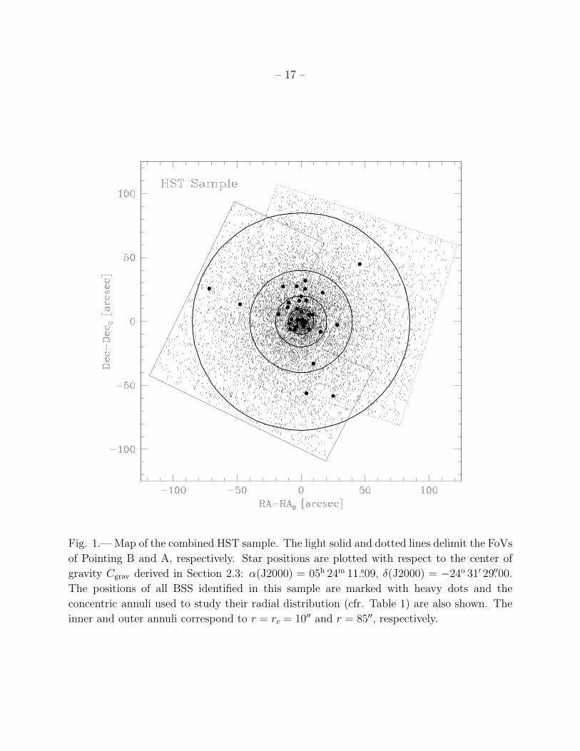
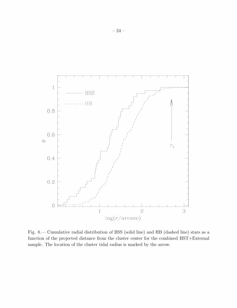
Beccari et al. 2006). In Figure 8 we compare the BSS cumulative radial distribution to that

of HB stars. The two distributions are obviously different, with the BSS being more centrally

concentrated than HB stars. A Kolmogorov-Smirnov test gives a ∼ 7×10−4 probability that

they are extracted from the same population, i.e. the two populations are different at more

than 3σ level.

For a more quantitative analysis, the surveyed area has been divided into 6 concentric

annuli, the first roughly corresponding to the core radius (r = 10′′), and the others chosen

in order to sample approximately the same fraction of the cluster luminosity out to the tidal

radius (rt ≃ 500′′). The luminosity in each annulus has been calculated by integrating the

surface density profile shown in Figure 4. The number of BSS and HB stars (NBSS and NHB,

respectively), as well as the fraction of sampled luminosity (Lsamp) measured in each annulus

are listed in Table 2 and have been used to compute the population ratio NBSS/NHB and the

– 10 –

specific frequencies (see Ferraro et al. 2003):

Rpop =(Npop/N

totpop)

(Lsamp/Lsamptot )

, (1)

with pop = BSS, HB.

The resulting radial trend of RHB over the surveyed area is essentially constant, with a

value close to unity (see Figure 9). This is just what expected on the basis of the stellar evolu-

tion theory, which predicts that the fraction of stars in any post-main sequence evolutionary

stage is strictly proportional to the fraction of the sampled luminosity (Renzini & Fusi Pecci

1988). In contrast the BSS show a completely different radial distribution: as shown in

Figure 9, the specific frequency RBSS is highly peaked at the cluster center decreases to a

minimum at r ≃ 12 rc and remains approximately constant outwards. The same behavior

is clearly visible also in Figure 10, where the population ratio NBSS/NHB is plotted as a

function of r/rc.

3.4. Dynamical simulations

Following the same approach as Mapelli et al. (2004, 2006) and Lanzoni et al. (2007),

we have used a Monte-Carlo simulation code (originally developed by Sigurdsson & Phinney

1995) in order to reproduce the observed radial distribution and to derive some clues about

the BSS formation mechanisms. Such a code follows the dynamical evolution of N BSS

within a background cluster, taking into account the effects of both dynamical friction and

distant encounters. Since stellar collisions are most probable in the central high-density

regions of the clusters, in the simulations we define COL-BSS those objects with initial

positions ri<∼ rc. Since primordial binaries most likely evolve in isolation if they orbit in

the cluster outskirts, we identify as MT-BSS those BSS having ri ≫ rc. Within these

defintions, in any given run we assume that a certain fraction of the N simulated BSS is

made of COL-BSS and the remaining fraction of MT-BSS. The initial positions ri of the

two types of BSS are randomly generated within the appropriate radial range (ri<∼ rc for

COL-BSS, and ri ≫ rc for the others) following a flat distribution, according to the fact

that the number of stars in a King model scales as dN = n(r) dV ∝ r−2πr2dr ∝ dr. Their

initial velocities are randomly extracted from the cluster velocity distribution illustrated

in Sigurdsson & Phinney (1995), and an additional natal kick is assigned to COL-BSS to

account for the recoil induced by the three-body encounters that trigger the merger and

produce the BSS (see, e.g., Sigurdsson, Davies & Bolte 1994; Davies, Benz & Hills 1994).

Each BSS has characteristic mass M and maximum lifetime tlast. We follow their dynamical

evolution in the (fixed) gravitational potential for a time ti (i = 1, N), where each ti is a

– 11 –

randomly chosen fraction of tlast. At the end of the simulation we register the final positions

of BSS, and we compare their radial distribution with the observed one. The percentage

of COL- and MT-BSS is changed and the procedure repeated until a reasonable agreement

between the simulated and the observed distributions is reached.

For a more detailed discussion of the procedure and the ranges of values appropriate for

the input parameters we refer to Mapelli et al. (2006). Here we only list the assumptions

made in the present study:

– the background cluster has been approximated with a multi-mass King model, deter-

mined as the best fit to the observed profile4. The cluster central velocity dispersion

is set to σ = 3.9 km s−1 (Dubath, Meylan & Mayor 1997), and, assuming 0.5 M⊙ as

the average mass of the cluster stars, the central stellar density is nc = 3 × 104 pc−3

(Pryor & Meylan 1993);

– BSS masses have been fixed to M = 1.2 M⊙ (see Section 3.2) and characteristic lifetimes

tlast ranging between 1.5 and 4 Gyr have been considered;

– COL-BSS have been distributed with initial positions ri ≤ rc and have been given a

natal kick velocity of 1 × σ;

– initial positions ranging between 5 rc and rt have been considered for MT-BSS in dif-

ferent runs;

– in each simulation we have followed the evolution of N = 10, 000 BSS.

The simulated radial distribution that best reproduces the observed one (with a reduced

χ2 ≃ 0.1) is shown in Figure 10 and is obtained by assuming that the totality of BSS is

made of COL-BSS. In the best-fit case the BSS characteristic lifetime is tlast ≃ 1.5 Gyr,

but a variation between 1 and 4 Gyr of this parameter still leads to a very good agreement

(χ2 ≃ 0.2–0.3) with the observations. For the sake of comparison, in Figure 10 we also show

the results of the simulations obtained by assuming a percentage of MT-BSS ranging from

10% to 40% (see lower and upper boundaries of the gray region, respectively)5. As can be

4By adopting the same mass groups as those of Mapelli et al. (2006), the resulting value of the King

dimensionless central potential is W0 = 10

5Note that a population of 40% MT-BSS was needed in order to reproduce the bimodal distribution

observed in M 3, 47 Tuc and NGC 6752 (Mapelli et al. 2006), and 10% was found to be the appropriate

percentage of MT-BSS in the case of M 5 (Lanzoni et al. 2007).

– 12 –

seen, while a population of 10% MT-BSS is still marginally consistent with the observations,

larger percentages systematically overestimate the BSS population at r >∼ 5 rc. Increasing

the BSS mass up to 1.5 M⊙ does not change this conclusion.

By assuming 12 Gyr for the age of NGC 1904, we have used the simulations and the

dynamical friction timescale (from, e.g., Mapelli et al. 2006) for 1.2 M⊙ stars to estimate

the radius of avoidance ravoid of the cluster, i.e., the radius within which all these stars are

expected to have already sunk to the cluster core because of mass segregation processes. We

find that ravoid ∼ 30 rc (i.e., ∼ 300′′), which corresponds to a significant fraction of the entire

cluster extension. This evidence is consistent with the fact that the simulated MT-BSS

appear to be a negligible fraction of the overall BSS population.

4. DISCUSSION

We have studied the brightest portion (m218 ≤ 19.5) of the BSS population in NGC 1904.

We have found a total of 39 objects, with a high degree of segregation in the cluster center.

Approximately 38% of the entire BSS population is found within the cluster core, while only

∼ 13% of HB stars are counted in the same region. This indicates a significant overabundance

of BSS in the center, as also confirmed by the fact that the BSS specific frequency RBSS within

rc is roughly 3 times larger than expected for a normal (non-segregated) population on the

basis of the sampled light (see Figure 9). The peak value is in good agreement with what is

found in the case of M 3, 47 Tuc, NGC 6752 and M 5 (see Ferraro et al. 2004; Sabbi et al.

2004; Lanzoni et al. 2007). Unlike these clusters, no significant upturn of the distribution

at large radii has been detected in NGC 1904.

We emphasize that the absence of an external upturn in the BSS radial distribution is

not an effect of low statistics. In the case of NGC 6752, where a similar amount of BSS (34)

has been detected, the BSS radial distribution is clearly bimodal (Sabbi et al. 2004). This

can be seen also in Figure 11, where the two distributions are directly compared. They nicely

agree within r ∼ 12rc, but the fraction of BSS in NGC 6752 rises again at larger distances

from the center, despite the smaller number of BSS observed in this cluster compared to

NGC 1904.

Extensive dynamical simulations have been used to derive some hints about the BSS

formation mechanisms. Even if admittedly crude, this approach has been successfully used to

demonstrate that the external rising branch of the BSS radial distribution observed in M 3,

47 Tuc, NGC 6752 and M 5 cannot be due to COL-BSS originated in the core and then kicked

out in the outer regions: hence, a significant fraction (20-40%) of the overall population is

– 13 –

required to be made of MT-BSS in these clusters (Mapelli et al. 2006; Lanzoni et al. 2007).

By using the same simulations to interpret the (flat) BSS radial distribution of NGC 1904,

we found that only a negligible percentage (0–10%) of MT-BSS is needed. However, we

emphasize that if a rising peripheral BSS frequency is absent (as in the case of NGC 1904)

our simple approach cannot distinguish between BSS created by MT (and then segregated

into the cluster core by the dynamical friction) and COL-BSS created by collisions inside

the core.

On the other hand, the negligible fraction of peripheral MT-BSS found in NGC 1904 is

in agreement with the quite large value of the radius of avoidance estimated for this cluster

(ravoid ≃ 30 rc), which indicates that all the heavy stars (binaries) within this radial distance

have had enough time to sink to the core and are therefore not expected in the cluster

outskirts. Such a radial distance corresponds to 0.6 rt, i.e., it represents a significant fraction

of the cluster extension (only 1% of the cluster light is contained between ravoid and rt),

and hence only a small fraction of the massive objects are expected to be unaffected by the

dynamical friction). In all the other studied cases, ravoid is significantly smaller: ravoid<∼ 0.2 rt

(Mapelli et al. 2006; Lanzoni et al. 2007). In turn, this suggests that at least a fraction of

the BSS population that we now observe in the cluster center are primordial binaries which

have sunk to the core because of the dynamical friction process, and mixed with those that

formed through stellar collisions.

Only systematic surveys of physical and chemical properties for a large number of BSS

in different environments (see examples in De Marco et al. 2005; Ferraro et al. 2006a) can

definitively identify the formation processes of these stars.

This research was supported by Agenzia Spaziale Italiana under contract ASI-INAF

I/023/05/0, by the Istituto Nazionale di Astrofisica under contract PRIN/INAF 2006, and

by the Ministero dell’Istruzione, dell’Universita e della Ricerca. RTR is partially funded by

NASA through grant number HST-GO-10524 from the Space Telescope Science Institute.

REFERENCES

Bailyn, C. D., & Pinsonneault, M. H. 1995, ApJ, 439, 705

Bailyn, C. D. 1995, ARA&A, 33, 133

Beccari, G., Ferraro, F. R., Lanzoni, B., & Bellazzini, M. 2006, ApJ, 652, L121

Buonanno, R., Buscema, G., Corsi, C. E., Ferraro, I., & Iannicola, G. 1983, A&A, 126, 278

– 14 –

Buonanno, R., Iannicola, G. 1989, PASP, 101, 294

Cariulo, P., Degl’Innocenti, S. & Castellani, V.,2003, A&A, 412, 1121

Carney, B. W., Latham, D. W., & Laird, J. B., 2005, AJ, 129, 466

Davies, M. B., Benz, W., & Hills, J. G. 1994, ApJ, 424, 870

De Marco, O., Shara, M. M., Zurek, D., Ouellette, J. A., Lanz, T., Saffer, R. A., & Sepinsky,

J.F. 2005, ApJ, 632, 894

Djorgovski, S. 1993, ASPC, 50, 373

Dorman, B., O’Connell, R. W., & Rood, R. T. 1995, ApJ442, 105

Dubath P., Meylan G., & Mayor M., 1997, A&A, 324, 505

Ferraro, F. R., Clementini, G., Fusi Pecci, F., Sortino, R., Buonanno, R. 1992, MNRAS256,

391

Ferraro, F. R., Paltrinieri, B., Fusi Pecci, F., Cacciari, C., Dorman, B., Rood, R. T., Buo-

nanno, R., Corsi, C. E., Burgarella, D., & Laget, M., 1997, A&A, 324, 915

Ferraro, F. R., Paltrinieri, B., Rood, R. T., Dorman, B. 1999a, ApJ 522, 983

Ferraro F. R., Messineo M., Fusi Pecci F., De Palo M. A., Straniero O., Chieffi A., Limongi

M. 1999b, AJ, 118, 1738

Ferraro, F. R., D’Amico, N., Possenti, A., Mignani, R. P., & Paltrinieri, B. 2001, ApJ, 561,

337

Ferraro, F. R., Sills, A., Rood, R. T., Paltrinieri, B., & Buonanno, R. 2003, ApJ, 588, 464

Ferraro, F. R., Beccari, G., Rood, R. T., Bellazzini, M., Sills, A., & Sabbi, E. 2004, ApJ,

603, 127

Ferraro, F. R., 2006, in Resolved Stellar Populations, ASP Conference Series, 2005, D. Valls-

Gabaud & M. Chaves Eds., astro-ph/0601217

Ferraro, F. R., et al. 2006a, ApJ, 647, L53

Ferraro, F. R., Sollima, A., Rood, R. T., Origlia, L., Pancino, E., & Bellazzini, M. 2006b,

ApJ, 638, 433

Harris, W.E. 1996, AJ, 112, 1487

– 15 –

Holtzman, J. A., Burrows, C. J., Casertano, S., Hester, J. J., Trauger, J. T., Watson, A. M.,

& Worthey, G. 1995, PASP, 107, 1065

Kravtsov, V., Ipatov, A., Samus, N., Smirnov, O., Alcaino, G., Liller, W., Alvarado, F. 1997,

A&A, 125, 1

Lanzoni, B., Dalessandro, E., Ferraro, F. R., Mancini, C., Beccari, G., Rood, R. T., Mapelli,

M., Sigurdsson, S. 2007, ApJin press (astro-ph/07040139)

Leigh, N., Sills, A., Knigge, C. 2007, ApJ in press (astro-ph/0702349)

Mapelli, M., Sigurdsson, S., Colpi, M., Ferraro, F. R., Possenti, A., Rood, R. T., Sills, A.,

& Beccari, G. 2004, ApJ, 605, L29

Mapelli, M., Sigurdsson, S., Ferraro, F. R., Colpi, M., Possenti, A., & Lanzoni, B. 2006,

MNRAS, 373, 361

Mateo, M., Harris, H. C., Nemec, J., Olszewski, E. W., 1990, AJ, 100, 469

McLaughlin, D. E., & van der Marel, R. P. 2005, ApJS, 161, 304

Montegriffo, P., Ferraro, F. R., Fusi Pecci, F., & Origlia, L. 1995, MNRAS, 276, 739

Pritchet, C. J., & Glaspey, J. W. 1991, ApJ, 373, 105

Pryor C., & Meylan G., 1993, Structure and Dynamics of Globular Clusters. Proceedings of a

Workshop held in Berkeley, California, July 15-17, 1992, to Honor the 65th Birthday of

Ivan King. Editors, S.G. Djorgovski and G. Meylan; Publisher, Astronomical Society

of the Pacific, Vol. 50, 357

Renzini, A., & Fusi Pecci, F. 1988, ARA&A, 26, 199

Sabbi, E., Ferraro, F. R., Sills, A., Rood, R. T., 2004, ApJ 617, 1296

Shara, M. M., Saffer, R. A., & Livio, M. 1997, ApJ, 489, L59

Sigurdsson, S., Davies, M. B., & Bolte, M. 1994, ApJ, 431, L115

Sigurdsson S., Phinney, E. S., 1995, ApJS, 99, 609

Stetson, P. B. 1987, PASP, 99, 191

Stetson, P. B. 2000, PASP, 112, 925, (for the photometric standards list see

http://cadcwww.hia.nrc.ca/standards/ )

– 16 –

Tian, B., Deng, L., Han, Z., Zhang, X. B. 2006, A&A 455, 247

Trager, S. C., Djorgovski, S.,& King, I. R. 1993, ASPC, 50, 347

Warren, S. R., Sandquist, E. L., & Bolte, M., 2006, ApJ 648, 1026

Zaggia, S. R., Piotto, G., & Capaccioli, M., 1997, A&A, 327, 1004

This preprint was prepared with the AAS LATEX macros v5.2.

– 17 –

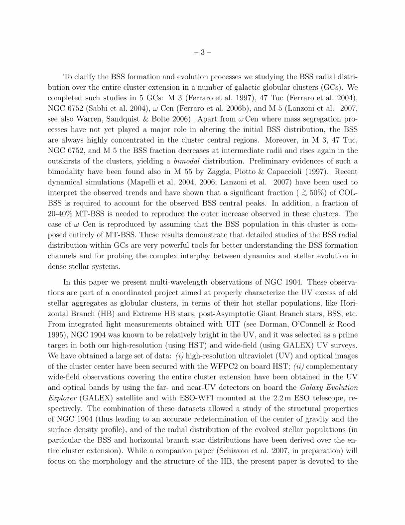
Fig. 1.— Map of the combined HST sample. The light solid and dotted lines delimit the FoVs

of Pointing B and A, respectively. Star positions are plotted with respect to the center of

gravity Cgrav derived in Section 2.3: α(J2000) = 05h 24m 11..s09, δ(J2000) = −24o 31′ 29.′′00.

The positions of all BSS identified in this sample are marked with heavy dots and the

concentric annuli used to study their radial distribution (cfr. Table 1) are also shown. The

inner and outer annuli correspond to r = rc = 10′′ and r = 85′′, respectively.

– 18 –

Fig. 2.— Map of the External sample. The light solid and dotted lines delimit the WFI and

the GALEX FoVs, respectively. The two BSS detected in the External sample are marked

as heavy dots, and the concentric annuli used to study their radial distribution are shown

as heavy circles. The inner annulus is at 85′′ and corresponds to the most external one in

Figure 1. The heavy dashed circle marks the tidal radius of the cluster (rt ≃ 500′′).

– 19 –

Fig. 3.— (V, B − V ) CMDs of the HST (Pointing B) and External samples. The hatched

regions (V ≥ 20) indicate the stars not used to derive the cluster surface density profile. The

adopted BSS and HB selection boxes are shown, and all the identified BSS are marked with

the empty circles.

– 20 –

Fig. 4.— Observed surface density profile (dots and error bars) and best-fit King model

(solid line). The radial profile is in units of number of stars per square arcsec. The dotted

line indicates the adopted level of the background, and the model characteristic parameters

(core radius rc, concentration c, dimensionless central potential W0), as well as the χ2 value

of the fit are marked in the figure. The location of the cluster tidal radius is marked by the

arrow. The lower panel shows the residuals between the observations and the fitted profile

at each radial coordinate.

– 21 –

Fig. 5.— CMD of the ultraviolet (Pointing B) HST sample. The adopted magnitude limit

and selection box used for the definition of the BSS population (empty circles) are shown.

The two solid triangles correspond to BSS-38 and 39 found in the External Sample, with

UV magnitudes obtained through the GALEX NUV detector. The selection boxes adopted

for HB and post-HB stars are also shown.

– 22 –

Fig. 6.— (V, U − V ) CMD of the HST (Pointing A) sample (only stars not observed in

Pointing B are plotted). The adopted BSS and HB selection boxes are shown, and all the

identified BSS and HB stars are marked with the empty circles and squares, respectively.

– 23 –

Fig. 7.— Upper panel: zoomed (V, B − V ) CMD of the BSS region; the 34 BSS measured

in this plane are shown. The set of isochrones ranging from 1 to 6 Gyr (stepped by 0.5 Gyr)

from Cariulo, Degl’Innocenti & Castellani (2003) data base used to derive BSS masses is

also shown. Lower panel: derived mass distribution for the BSS shown in the upper panel.

– 24 –

Fig. 8.— Cumulative radial distribution of BSS (solid line) and HB (dashed line) stars as a

function of the projected distance from the cluster center for the combined HST+External

sample. The location of the cluster tidal radius is marked by the arrow.

– 25 –

Fig. 9.— Radial distribution of the BSS (dots) and HB (gray regions) specific frequencies,

as defined in equation (1), and as a function of the radial distance in units of the core radius.

The vertical size of the gray regions correspond to the error bars.

– 26 –

Fig. 10.— Radial distribution of the population ratio NBSS/NHB as a function of r/rc (dots

with error bars), compared with the simulated distribution (solid line and triangles) obtained

by assuming 100% of COL-BSS. The results of the simulations obtained by assuming a

percentage of MT-BSS ranging from 10% to 40% (lower and upper boundaries of the gray

region, respectively) are also shown.

– 27 –

Fig. 11.— Radial distribution of the population ratio NBSS/NHB for NGC 1904 (filled circles)

and NGC 6752 (open circles) plotted as a function of the radial distance in core radius units.

– 28 –

Table 1. The BSS population in NGC1904

Name RA DEC m218 U B V I

[degree] [degree]

BSS-1 81.048797100 -24.526391100 19.11 18.64 18.66 18.45 -

BSS-2 81.047782800 -24.526527400 18.65 18.12 18.21 17.94 -

BSS-3 81.047540400 -24.526005300 18.85 18.34 18.38 18.22 -

BSS-4 81.048954000 -24.525188200 17.94 17.75 17.87 17.78 -

BSS-5 81.047199200 -24.525797600 17.58 17.47 17.40 17.35 -

BSS-6 81.045528300 -24.525876800 18.64 18.24 18.28 18.12 -

BSS-7 81.044296100 -24.526362200 19.13 18.77 18.76 18.55 -

BSS-8 81.048506700 -24.524266800 19.18 18.55 18.64 18.39 -

BSS-9 81.041556100 -24.526972400 19.35 18.65 18.86 18.49 -

BSS-10 81.045827300 -24.525062700 18.06 17.35 17.17 16.96 -

BSS-11 81.045467700 -24.525147900 17.84 17.44 17.56 17.41 -

BSS-12 81.047088300 -24.524375900 18.80 18.20 18.01 17.80 -

BSS-13 81.046548400 -24.524483700 19.43 18.77 18.67 18.38 -

BSS-14 81.045121300 -24.524748300 19.28 18.33 18.65 18.21 -

BSS-15 81.045883300 -24.524278600 18.97 18.42 18.30 18.13 -

BSS-16 81.046164500 -24.522567300 18.41 17.72 17.63 17.42 -

BSS-17 81.044313700 -24.523304200 18.66 18.46 18.44 18.27 -

BSS-18 81.047157500 -24.521982700 18.49 18.45 18.41 18.32 -

BSS-19 81.043418100 -24.523247200 17.88 18.16 17.68 17.55 -

BSS-20 81.046665900 -24.520192000 19.49 18.71 18.92 18.60 -

BSS-21 81.044991400 -24.520127500 18.93 18.45 18.44 18.21 -

BSS-22 81.046157800 -24.519245100 19.49 18.92 19.06 18.74 -

BSS-23 81.049326100 -24.521621900 18.08 - 18.01 17.99 -

BSS-24 81.049155900 -24.520629500 18.41 - 17.98 17.87 -

BSS-25 81.047244500 -24.517052600 19.41 18.97 19.11 18.82 -

BSS-26 81.051592200 -24.523146600 18.67 - 18.33 18.21 -

BSS-27 81.050476100 -24.517107000 19.01 18.65 18.54 18.39 -

BSS-28 81.060767000 -24.520983900 18.92 - 18.59 18.45 -

BSS-29 81.068117100 -24.517558600 19.39 - 18.91 18.60 -

BSS-30 81.043233100 -24.533852000 17.34 - 16.75 16.65 -

BSS-31 81.044917900 -24.540315000 18.34 - 17.48 17.22 -

BSS-32 81.038520800 -24.540891600 17.77 17.46 17.30 17.20 -

BSS-33 81.045196533 -24.515874863 - 17.91 - 17.84 -

BSS-34 81.032196045 -24.512256622 - 18.75 - 18.41 -

BSS-35 81.037574768 -24.525493622 - 18.87 - 18.58 -

BSS-36 81.041069031 -24.518457413 - 18.80 - 18.64 -

BSS-37 81.045227051 -24.517648697 - 18.86 - 18.68 -

BSS-38 81.056510925 -24.449676514 19.04† 18.78 18.56 18.35 18.08

– 29 –

Table 1—Continued

BSS-39 81.058883667 -24.555763245 19.39† 19.14 19.05 18.73 18.34

Note. — † Note that, while the header of the column referes to HST-F218W

magnitudes, those of BSS-38 and -39 have been obtained with the NUV channel

of GALEX and transformed to the m218 scale as described in Section 2.2.

ri re NBSS NHB Lsamp/Lsamptot

0 10 15 34 0.14

10 20 10 45 0.18

20 40 7 62 0.22

40 85 5 56 0.23

85 150 1 34 0.13

150 500 1 18 0.10

Table 2: Number of BSS and HB stars, and fraction of luminosity sampled in the 6 concentric

annuli used to study the BSS radial distribution of NGC 1904 (ri and re correspond to the

internal and external radius of each considered annulus, in arcsec).