arX

iv:1

009.

0649

v1 [

astr

o-ph

.GA

] 3

Sep

201

0Draft version September 6, 2010Preprint typeset using LATEX style emulateapj v. 11/10/09

LIGHT-ELEMENT ABUNDANCE VARIATIONS AT LOW METALLICITY: THE GLOBULAR CLUSTER NGC5466

Matthew ShetroneMcDonald Observatory, University of Texas at Austin, HC75 Box 1337-MCD, Fort Davis, TX 79734, USA

Sarah L. MartellAstronomisches Rechen-Institut, Zentrum fur Astronomie der Universitat Heidelberg, Monchhofstr. 12-14, D-69120 Heidelberg,

Germany

Rachel WilkersonCenter for Astrophysics, Space Physics and Engineering Research One Baylor Place #97310, Baylor University Waco, TX 76798-7310,

USA

Joshua AdamsAstronomy Department, University of Texas at Austin, Austin, TX 78712, USA

Michael H. SiegelDepartment of Astronomy and Astrophysics, Pennsylvania State University, 525 Davey Laboratory, State College, PA 16801, USA

Graeme H. SmithUniversity of California Observatories / Lick Observatory, Department of Astronomy & Astrophysics, UC Santa Cruz, 1156 High St.,

Santa Cruz, CA 95064, USA

and

Howard E. BondSpace Telescope Science Institute, 3700 San Martin Dr, Baltimore, MD 21218, USA

Draft version September 6, 2010

ABSTRACT

We present low-resolution (R≃ 850) spectra for 67 asymptotic giant branch, horizontal branch and redgiant branch (RGB) stars in the low-metallicity globular cluster NGC 5466, taken with the VIRUS-Pintegral-field spectrograph at the 2.7-m Harlan J. Smith telescope at McDonald Observatory. Sixty-sixstars are confirmed, and one rejected, as cluster members based on radial velocity, which we measureto an accuracy of 16 km s−1via template-matching techniques. CN and CH band strengths have beenmeasured for 29 RGB and AGB stars in NGC 5466, and the band strength indices measured fromVIRUS-P data show close agreement with those measured from Keck/LRIS spectra previously takenof five of our target stars. We also determine carbon abundances from comparisons with syntheticspectra. The RGB stars in our data set cover a range in absolute V magnitude from +2 to −3,which permits us to study the rate of carbon depletion on the giant branch as well as the point of itsonset. The data show a clear decline in carbon abundance with rising luminosity above the luminosityfunction “bump” on the giant branch, and also a subdued range in CN band strength, suggestingongoing internal mixing in individual stars but minor or no primordial star-to-star variation in light-element abundances.Subject headings: globular clusters: general - globular clusters: individual (NGC 5466) - stars: abun-

dances

1. INTRODUCTION

In all Galactic globular clusters with moderate metal-licity ([Fe/H] ≃ −1.5), there are star-to-star variationsin the strength of the 3883A CN absorption band at anygiven evolutionary phase. These CN band strengths an-

shetrone@astro.as.utexas.edumartell@ari.uni-heidelberg.derachelw52@gmail.comjjadams@astro.as.utexas.edusiegel@astro.psu.edugraeme@ucolick.orgbond@stsci.edu

ticorrelate with CH band strengths, so that stars withweak CH bands (and therefore relatively low carbonabundances) have strong CN bands (and therefore rel-atively high nitrogen abundances). Band-strength varia-tions were first observed in spectra of red giants in globu-lar clusters (e.g., Norris & Freeman 1979, Suntzeff 1981),but are also found in subgiants and on the main sequence(e.g., Briley et al. 2004), indicating that they are a resultof primordial enrichment rather than an evolutionary ef-fect.Variations in the broad CN and CH features are just

the most readily observed part of a larger light-element

2

abundance pattern, a division of globular cluster starsinto one group with typical Population II abundancesand another that is relatively enhanced in nitrogen,sodium, and aluminum, and depleted in carbon, oxy-gen, and magnesium. These abundance divisions areusually studied in the anticorrelated pairs of carbon andnitrogen or oxygen and sodium (see, e.g., Kraft 1994;Gratton et al. 2004; Carretta et al. 2009). Themagnesium-aluminum anticorrelation is more murky: al-though some researchers find Mg-Al anticorrelations inindividual globular clusters (e.g., Shetrone 1996; Grat-ton et al. 2001), the abundance distributions are not asclearly bimodal as in the case of nitrogen, and the ori-gin of Mg-poor, Al-rich stars is more difficult to fit intothe general framework of enrichment by moderate-massAGB stars (e.g., D’Ercole et al. 2008).This paper presents a study of the behavior of CN and

CH band strengths and [C/Fe] abundances in red giantstars in the low-metallicity globular cluster NGC 5466,which has [Fe/H] ≃ 2.2 (Harris 1996, 2003 revision).Studies based on CN and CH band strength are more dif-ficult in low-metallicity clusters, where the CN variationvisible in the spectra can be quite small despite variationsin [N/Fe] abundance as large as in higher-metallicityglobular clusters (e.g., M53, Martell et al. 2008a; M55,Briley et al. 1993). The globular clusters with metallic-ities similar to NGC 5466 in which light-element abun-dance inhomogeneities have been most extensively stud-ied are M92 and M15. The red giants in both objectsexhibit a progressive decline in [C/Fe] with advancingevolution above the magnitude level of the horizontalbranch (HB; Carbon et al. 1982; Trefzger et al. 1983;Langer et al. 1986; Bellman et al. 2001). Giants in bothclusters typically exhibit weak λ3883 CN bands (Carbonet al. 1982; Trefzger et al. 1983), and do not exhibitbimodal CN distributions like those in more metal-richclusters although a handful of stars with enhanced CNhave been discovered in M15 (Langer, Suntzeff, & Kraft1992; Lee 2000). Despite their lack of CN-strong giants,both M92 and M15 exhibit anticorrelated O-N, O-Na orO-Al variations, or correlated N-Na, of the type that arecommonplace in globular clusters (Norris & Pilachowski1985; Sneden et al. 1991, 1997; Shetrone 1996). In ad-dition, Cohen, Briley & Stetson (2005) discovered thatstar-to-star differences in [C/Fe] and [N/Fe] abundancesexist among stars near the base of the red giant branch(RGB) in M15, and the C and N abundances tend to beanticorrelated. These efforts have shown that for verymetal-poor stars the use of CN to determine which starscarry the anticorrelated light-element abundance patterncan be problematic, and that anticorrelated variationsin light-element abundances do exist in low-metallicityglobular clusters despite their lack of obvious CN bandstrength variation.If NGC 5466 does contain the same primordial varia-

tions in light-element abundances as are found in higher-metallicity globular clusters, the resulting range in CNand CH band strength will be muted by the low overallmetallicity of the cluster, perhaps to a degree where it isdifficult to distinguish a bimodal but closely spaced CNband strength distribution from a broad but unimodaldistribution. If NGC 5466 does not contain primordialabundance variations, that would imply that primordialenrichment is not a universal process in low-metallicity

globular clusters the way it is in higher-metallicity clus-ters. A metallicity limit on primordial light-element en-richment offers some insight into the primordial enrich-ment process, and into the larger and still-developingpicture of chemical complexity within individual globu-lar clusters (e.g., Piotto 2008).

2. OBSERVATIONS AND REDUCTION

We determined photometry for members of NGC 5466based on CCD frames obtained by HEB with the KittPeak National Observatory 0.9 m telescope on 1997 May9. The T2KA chip at the Ritchey-Chretien focus pro-vides a 23′ × 23′ field, which encloses most of the clus-ter, which has a tidal radius of 34′, according to Harris(1996). We used uBV I filters, as defined by Bond (2005),with exposure times of 600, 45, 45, and 60 s, respectively,under photometric conditions. We calibrated the pho-tometry to the network of uBV I standard stars estab-lished by Siegel & Bond (2005). Data were reduced usingthe IRAF CCDPROC pipeline and photometry was mea-sured with DAOPHOT/ALLSTAR (Stetson 1987, 1994).DAOGROW (Stetson 1990) was used to perform curve-of-growth fitting for aperture correction on both programand standard stars. The raw photometry was calibratedusing the iterative matrix inversion technique describedin Siegel et al. (2002) to translate the photometry to thestandard system of Landolt (1992) and Siegel & Bond(2005). Table 1 lists identification numbers, positions,and photometry for the stars observed with VIRUS-P.The star identification numbers and coordinates are froman unpublished photometric catalog developed by M.H.S.from the analysis described above. The typical errors onthe B, V, and I photometry are 0.030, 0.022 and 0.032mag, respectively.On 2009 March 3–5 and July 28–29, we observed four

fields in NGC 5466 for a total of 22 hr with the visi-ble integral-field replicable unit spectrograph prototype(VIRUS-P, Hill et al. 2008) on the 2.7m Harlan J. SmithTelescope at McDonald Observatory. VIRUS-P is a spec-trograph with an integral field unit (IFU) of 246 fibersin a hexagonal, one third fill factor, close pack pattern.The fibers have a projected diameter of 4.1′′ and havecenters astrometrically calibrated to 0.7′′ relative to afixed, offset guiding camera via open cluster observa-tions. The field of view for the IFU is 2.89 square arcminand with a set of three 7.14” dithers the filling factor is100%. The VP1 grating was used, giving an instrumen-tal FWHM between 5 and 6A over the wavelength rangeof 3500− 5800A. Arc lamp calibration produced a wave-length solution with an rms accuracy of 0.05A. Our pro-cedure during observing was to dither the telescope andtake three 1200 s exposures per field to fill in the spacesbetween the IFU fibers. Three of the fields had four setsof dithers, but the July observing run was less successfuldue to weather and only a single dither set was taken forthe final field.A custom software pipeline developed for the instru-

ment (Adams 2010, in preparation) was used in all re-ductions. The notable features are that no interpolationwas performed on the data to avoid correlated noise andthat background subtraction was done between differ-ently sampled fibers by fitting B-spline models (Dierckx1993) in a running boxcar of 31 chip-adjacent fibers in amanner similar to optimal longslit sky subtraction meth-

3

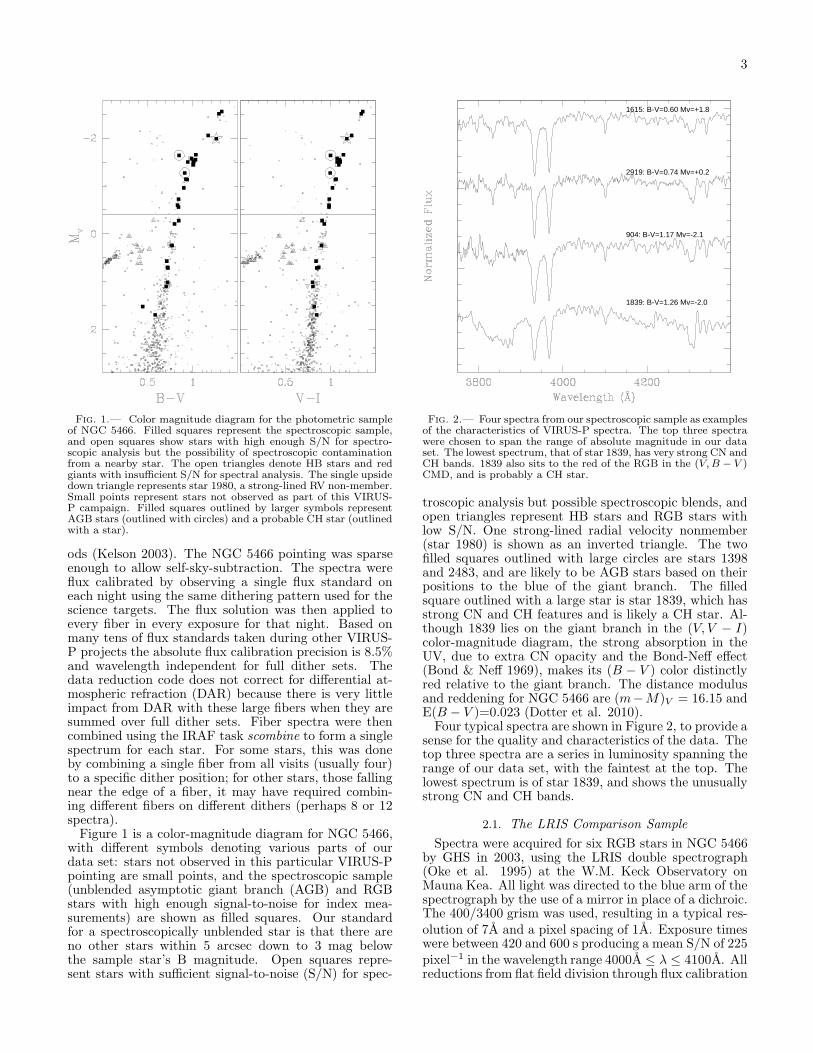
Fig. 1.— Color magnitude diagram for the photometric sampleof NGC 5466. Filled squares represent the spectroscopic sample,and open squares show stars with high enough S/N for spectro-scopic analysis but the possibility of spectroscopic contaminationfrom a nearby star. The open triangles denote HB stars and redgiants with insufficient S/N for spectral analysis. The single upsidedown triangle represents star 1980, a strong-lined RV non-member.Small points represent stars not observed as part of this VIRUS-P campaign. Filled squares outlined by larger symbols representAGB stars (outlined with circles) and a probable CH star (outlinedwith a star).

ods (Kelson 2003). The NGC 5466 pointing was sparseenough to allow self-sky-subtraction. The spectra wereflux calibrated by observing a single flux standard oneach night using the same dithering pattern used for thescience targets. The flux solution was then applied toevery fiber in every exposure for that night. Based onmany tens of flux standards taken during other VIRUS-P projects the absolute flux calibration precision is 8.5%and wavelength independent for full dither sets. Thedata reduction code does not correct for differential at-mospheric refraction (DAR) because there is very littleimpact from DAR with these large fibers when they aresummed over full dither sets. Fiber spectra were thencombined using the IRAF task scombine to form a singlespectrum for each star. For some stars, this was doneby combining a single fiber from all visits (usually four)to a specific dither position; for other stars, those fallingnear the edge of a fiber, it may have required combin-ing different fibers on different dithers (perhaps 8 or 12spectra).Figure 1 is a color-magnitude diagram for NGC 5466,

with different symbols denoting various parts of ourdata set: stars not observed in this particular VIRUS-Ppointing are small points, and the spectroscopic sample(unblended asymptotic giant branch (AGB) and RGBstars with high enough signal-to-noise for index mea-surements) are shown as filled squares. Our standardfor a spectroscopically unblended star is that there areno other stars within 5 arcsec down to 3 mag belowthe sample star’s B magnitude. Open squares repre-sent stars with sufficient signal-to-noise (S/N) for spec-

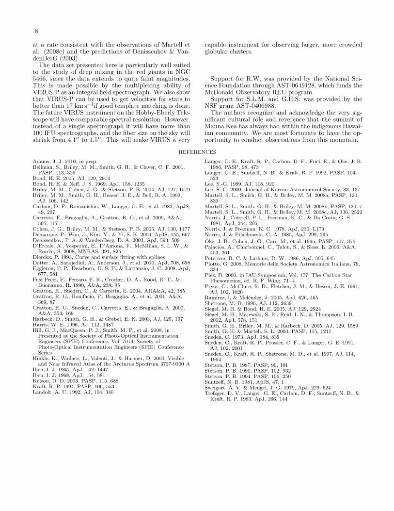
1615: B-V=0.60 Mv=+1.8

2919: B-V=0.74 Mv=+0.2

904: B-V=1.17 Mv=-2.1

1839: B-V=1.26 Mv=-2.0

Fig. 2.— Four spectra from our spectroscopic sample as examplesof the characteristics of VIRUS-P spectra. The top three spectrawere chosen to span the range of absolute magnitude in our dataset. The lowest spectrum, that of star 1839, has very strong CN andCH bands. 1839 also sits to the red of the RGB in the (V,B − V )CMD, and is probably a CH star.

troscopic analysis but possible spectroscopic blends, andopen triangles represent HB stars and RGB stars withlow S/N. One strong-lined radial velocity nonmember(star 1980) is shown as an inverted triangle. The twofilled squares outlined with large circles are stars 1398and 2483, and are likely to be AGB stars based on theirpositions to the blue of the giant branch. The filledsquare outlined with a large star is star 1839, which hasstrong CN and CH features and is likely a CH star. Al-though 1839 lies on the giant branch in the (V, V − I)color-magnitude diagram, the strong absorption in theUV, due to extra CN opacity and the Bond-Neff effect(Bond & Neff 1969), makes its (B − V ) color distinctlyred relative to the giant branch. The distance modulusand reddening for NGC 5466 are (m−M)V = 16.15 andE(B − V )=0.023 (Dotter et al. 2010).Four typical spectra are shown in Figure 2, to provide a

sense for the quality and characteristics of the data. Thetop three spectra are a series in luminosity spanning therange of our data set, with the faintest at the top. Thelowest spectrum is of star 1839, and shows the unusuallystrong CN and CH bands.

2.1. The LRIS Comparison Sample

Spectra were acquired for six RGB stars in NGC 5466by GHS in 2003, using the LRIS double spectrograph(Oke et al. 1995) at the W.M. Keck Observatory onMauna Kea. All light was directed to the blue arm of thespectrograph by the use of a mirror in place of a dichroic.The 400/3400 grism was used, resulting in a typical res-olution of 7A and a pixel spacing of 1A. Exposure timeswere between 420 and 600 s producing a mean S/N of 225pixel−1 in the wavelength range 4000A ≤ λ ≤ 4100A. Allreductions from flat field division through flux calibration

4

Fig. 3.— Radial velocities for all stars in our photometric sample,with a horizontal dashed line marking the mean velocity of 118.0km s−1. The horizontal solid line represents the mean cluster radialvelocity values taken from Peterson & Latham (1986) and Pryoret al. (1991). The error on our mean velocity is 0.4 km s−1, andthe rms is 17.0 km s−1. This rms is 5% of a resolution elementwith VIRUS-P. The single inverted triangle represents star 1980, astrong-lined star that is also a radial velocity non-member.

were carried out using the XIDL routines developed byJ.X. Prochaska.

3. RADIAL VELOCITY AND MEMBERSHIP

For radial velocity determinations, data were cross-correlated with a template spectrum: for RGB and AGBstars, the template was the Hinkle Arcturus atlas (Hin-kle et al. 2000) convolved with a Gaussian to createan R = 850 spectrum. The HB star template was gen-erated from a synthetic spectrum with Teff= 6000 K,log(g)= 3.00 dex and [Fe/H]= −2.0 dex.Figure 3 shows the distribution of our velocity mea-

surements. The weighted average is 118.0 ± 0.4km s−1with an rms of 17.0 kms−1. This rms is 5% of aresolution element with VIRUS-P. More customized tem-plate spectra may allow improvements in the rms scatter.The mean of literature values for the systemic velocityof NGC 5466 is 108 km s−1(Harris 1996), and solid hori-zontal lines in Figure 4 show velocities from Pryor et al.(1991) and Peterson & Latham (1986). The individualstar radial velocities are listed in Table 1. In the fol-lowing analysis, spectra are individually shifted to restwavelengths according to these radial velocities.

4. BAND STRENGTHS AND BIMODALITY

CN and CH band strengths are typically quantifiedwith indices that measure the magnitude difference be-tween the integrated flux within the feature in questionand the integrated flux in one or two nearby continuumregions, in the sense that more absorption in the featureproduces a larger band-strength index. For CN bandstrength, we measure the index S(3839), defined in Nor-ris et al. (1981) as

S(3839) = −2.5 log

∫ 3916

3883Iλdλ

∫ 3883

3846 Iλdλ(1)

-0.1

-0.05

0

0.05

0.1

2635 3176 727 1320 2891 2635 3176 727 1320 2891

Fig. 4.— Comparison of band indices measured from the KeckLRIS spectra discussed in Section 2.1 and those measured fromVIRUS-P spectra, for the five stars in common to both data sets.Identification numbers are given at the bottom of each panel.

The index we use for CH band strength is S2(CH), de-fined in Martell et al. (2008b) as

S2(CH) = −2.5 log

∫ 4317

4297 Iλdλ∫ 4242

4212Iλdλ+

∫ 4375

4330Iλdλ

(2)

Band-strength indices tend to be designed to be effec-tive for a single stellar population, for example CH(4300)(Harbeck et al. 2003, designed for main-sequence starsin 47 Tucanae) and CH(G) (Lee 1999, designed forbright red giants in M3), and can be difficult to ap-ply outside the parameter space for which they were in-tended. S2(CH) was specifically designed to be sensitiveto variations in carbon abundance in bright red giants(MV ≤ −1.0) across a wide range of metallicity, andtherefore ought to be valid for the sample at hand.The errors on our band strengths have two compo-

nents, errors related to the fluxing and errors related tothe S/N. S/N errors were calculated by propagating thePoisson noise errors through the formulas for the bandindices. To estimate the errors in our fluxing we triedseveral techniques to reflux the data including using syn-thetic spectra matched to each star’s photometric tem-perature and using average flux distributions for colorbins along the giant branch. The two sources of errorwere added in quadrature, and the total errors are re-ported in Table 2 as σS and σS2 for S(3839) and S2(CH),respectively. For the March observing run the S/N in theS2(CH) band was quite high and the fluxing errors domi-nate while for the July observing run, where only a singledither set was taken for the final fourth field, the Poissonnoise contribution plays a significant contribution to thetotal error. For S(3839), the Poisson error tends to dom-inate the total error in all cases. Errors in radial velocityare typically 17 km s−1, or 5% of a pixel, as mentionedin Section 3, and do not have a significant effect on mea-sured band strengths. Shifting our wavelengths to theblue or red by 17 km s−1changes the measured S2(CH)by 0.001 mag, which is small relative to the fluxing- andnoise-related errors in S2(CH).Five of the stars in the LRIS data set are also in the

VIRUS-P spectroscopic sample, and the CN and CH

5

Fig. 5.— CN band-strength index S(3839) vs. absolute V mag-nitude, for all stars in our spectroscopic sample. The solid line is aleast-squares fit, and we classify stars that lie above the line (shownas filled squares) as relatively CN-strong and stars that lie belowthe line (drawn as open squares) as relatively CN-weak. Small tri-angles denote stars with sufficient S/N for spectroscopic analysisbut possible spectroscopic blending. The clear outlier, outlinedwith a large open star, is star 1839, noted in Figure 2 as a proba-ble CH star. The two points outlined with large open circles (stars1398 and 2483) lie to the blue of the RGB in Figure 1, and arelikely AGB stars.

band strengths measured from the LRIS spectra are quitesimilar to band strengths measured from the VIRUS-Pdata. Figure 4 shows ∆S(3839) and ∆S2(CH) for thestars in common between the two data sets, in the senseLRIS−VIRUS-P, and differences between the two datasets are quite small. The band strengths given in Table2 come exclusively from the VIRUS-P data.Since the 3883A CN band strength can be used as a

proxy for nitrogen abundance, and the 4320A CH bandstrength for carbon abundance, a comparison of CN andCH band strength in a globular cluster ought to re-veal anticorrelated abundance behavior. As can be seenin Figure 5, the CN band strength in our sample risesslightly with rising luminosity, but does not show a largerange at fixed MV . The clear outlier, with a large openstar drawn around it, is star 1839, the star with the un-usually strong CN and CH features in Figure 2. It isexcluded from the rest of our band strength and abun-dance analysis.The S(3839) band strengths are correlated, to first or-

der, with luminosity. To better distinguish stars that areCN-weak from stars that are CN-strong, we fit a linear re-lationship between S(3839) and MV and evaluated eachstar based on its vertical distance from this linear rela-tionship (δS(3839)). We divide the sample into relativelyCN-weak (negative δS(3839), open squares) and CN-strong (positive δS(3839), solid squares) stars. Unlike instudies of higher-metallicity globular clusters (see Norriset al. 1981 for a typical example), there is not a clear gapbetween the relatively CN-weak and CN-strong groups.In Figure 6 we compare δS(3839) and S2(CH) bandstrengths, with the same symbols (open/solid squares)representing CN class, and there is not a strong anticor-relation between CN class and CH band strength. Thetwo large crosses are centered at the mean values forδS(3839) and S2(CH) for the two groups, with their sizeset to equal the standard deviations. They are not ob-

Fig. 6.— CN band-strength index δS(3839) vs. CH band-strength index S2(CH), for the spectroscopic sample. The symbolsare the same as in Figure 5. The large crosses are centered at themean values of δS(3839) and S2(CH) for the CN-weak and CN-strong groups, and their sizes are the standard deviations of theindices. CN and CH band strengths are typically anticorrelatedin globular cluster stars, indicating anticorrelated carbon and ni-trogen abundances. The lack of strong anticorrelation here is theresult of a smaller than typical range in CN band strength in NGC5466, and possibly a smaller range in [C/Fe] and [N/Fe] than inhigher-metallicity globular clusters.

viously offset from each other in S2(CH). This may besimply an effect of the extremely limited range in CN andCH band strengths permitted by the low overall metal-licity of NGC 5466.Another way to visualize the distribution of CN band

strength in our data set is the generalized histogram,which is constructed by representing each star as a Gaus-sian in δS(3839) with a width equal to the measurementerror σS , and then summing the individual Gaussians.The result is shown in Figure 7, in which the solid curveis the generalized histogram for the full data set andthe dashed curves are the generalized histograms cal-culated just for the relatively CN-weak and CN-stronggroups. The upper panel of Figure 8 shows the singleGaussian that best fits the generalized histogram fromFigure 7, and the lower panel, showing the residual be-tween the best-fit curve and the data, shows a clearlydouble-peaked shape. This double-peaked residual sug-gests the system is better fit by two Gaussians.Based on our analysis of the generalized histogram, we

claim that NGC 5466 contains two closely spaced groupsin CN band strength, a result of intrinsic ranges in car-bon and nitrogen abundance and low overall metallic-ity. The lack of a gap in CN band strength betweenthe two groups of stars in Figure 5 is seen here as afairly small distance between the peaks of the CN-weakand CN-strong generalized histograms. Similarly metal-poor globular clusters such as M15 (Lee 2000) and M53(Martell et al. 2008a) also exhibit small separations be-tween their CN-weak and CN-strong groups and a smalloverall range in S(3839) (among red giants in the threeclusters δS(3839) has a standard deviation of 0.038 inNGC 5466, 0.056 in M53, and 0.037 in M15). This sug-gests that the range of carbon and nitrogen abundancein low-metallicity globular clusters may be smaller thanis typical for more moderate-metallicity clusters. In ad-dition, since the measurement errors on S(3839) control

6

Fig. 7.— Solid curve is a generalized histogram for theluminosity-independent CN band strength measure δS(3839) mea-sured for our full spectroscopic sample, and the dashed curves aregeneralized histograms for δS(3839) in the relatively CN-weak andCN-strong groups calculated independently.

the widths of the individual Gaussians comprising thegeneralized histogram, they can have strong effects onour interpretation of it, with very large measurement er-rors potentially rendering two closely spaced populationsindistinguishable from a single broad distribution.To understand the effects of measurement error on our

generalized histogram, we performed a Monte Carlo testexploring how the size of our measurement errors af-fects the Kolmogorov-Smirnov coefficient p, which quan-tifies the probability that the CN-strong and CN-weakgroups were drawn from the same initial population. Werescaled our true measurement errors σS by factors rang-ing from 0.5 to 10, then selected a new value for each datapoint from within a Gaussian distribution centered at themeasured value of δS(3839), with a width of the rescaledmeasurement error. This reselection was done for theCN-normal and CN-strong groups identified in Figure 4independently. The K-S p coefficient was then measuredas an indicator of whether the two CN band strengthgroups containing reselected points with rescaled errorsseemed likely to have been drawn from the same initialpopulation. Reselections were done 104 times for eachrescaling of the measurement error, and we find that p isstrongly concentrated near zero when the rescaling fac-tor is relatively small: for a rescaling factor of 1, 99%of realizations have a p less than 0.1 and none have a plarger than 0.61, and 82% of realizations with a rescalingfactor of 3 have a p less than 0.5. With a rescaling factorof 10, we find that p values are fairly evenly distributedbetween 0 and 1, with 51% below p = 0.5. Based onthis test, we are fairly confident that our two CN groupsreally are distinct, even if our errors in S(3839) are un-derestimated by a factor of 3.

5. EVOLUTION OF CARBON ABUNDANCE

Carbon abundances were determined by spectral syn-thesis of the G-band region. For each star, a set of syn-thetic spectra were created with a single Teff , log(g),and [Fe/H], and a range of possible values for [C/Fe],smoothed to the resolution of the VIRUS-P data. Thesynthetic spectra were generated using a modified versionof MOOG 2009 (Sneden 1973) which generates fluxed

0

5

10

15

-0.2 -0.1 0 0.1 0.2

-1

-0.5

0

0.5

1

Fig. 8.— Upper panel shows the generalized histogram fromFigure 7 as a solid line, with a simple Gaussian fit to the distri-bution overplotted as a dotted line. The lower panel shows thedifference between the two curves, and there is a clear two-peakedshape, which suggests that the data are best represented as twooverlapping Gaussian distributions.

spectra instead of normalized spectra. We used thePLEZ2000 grid of metal-poor model atmospheres (Plez2000). The temperatures and surface gravities were de-rived from the photometry in Table 1 using the prescrip-tions in Ramırez & Melendez (2005). We adopted [α/Fe]= 0.3, 12C/13C= 6 and [Fe/H] = −2.0 for all stars. Thechoice of the carbon isotope ratio does make a smalldifference to the derived total carbon abundance. Atthese metallicities, where the lines are reasonably weak,a change of 12C/13C from 6 to 50 would make about 0.06dex difference to [C/Fe] which is much smaller than thequoted errors. The synthetic spectrum yielding the resid-ual (in the sense observed - synthetic) that is closest tozero in the region of the CH G-band was chosen to havethe correct carbon abundance. Table 2 lists ID numbers,VIRUS-P CN and CH band strengths, and carbon abun-dances along with their associated errors for the stars inthe spectroscopic sample and for those that have goodS/N but are possibly spectroscopically blended.Observational studies of CH band strengths and [C/Fe]

abundances in red giants in globular clusters and in thefield (e.g., Gratton et al. 2000; Smith & Martell 2003;Smith et al. 2005) have shown clearly that bright, low-mass red giants in all Galactic environments experiencesteady carbon depletion as they evolve along the giantbranch. This depletion only occurs in stars brighter thanthe “bump” in the RGB luminosity function, and pro-ceeds at a rate that is metallicity-dependent. The homo-geneity and wide luminosity range of our spectroscopicsample makes it very useful for careful study of the rateand point of onset of deep mixing in NGC 5466.The first dredge-up process that occurs when a star

moves on to the RGB (Iben 1965, 1968) is caused by thebase of the convective envelope dropping in to small ra-dius, until hydrogen shell burning ignites, equilibrates,

7

Fig. 9.— Upper panel shows the CH band-strength indexS2(CH) as a function of absolute V magnitude, and the usualglobular cluster pattern of a plateau at low luminosity, followed bya decline in stars brighter than the ”bump” in the RGB luminosityfunction, is apparent. The vertical line marks the position of theRGB bump at this metallicity. The lower panel shows our calcu-lated [C/Fe] abundances, which also exhibit a plateau followed bya steady evolutionary decline. As discussed in the text, the rate ofcarbon depletion measured in NGC 5466 is consistent with the low-metallicity carbon depletion rate found in Martell et al. (2008c).

and restores the stability against convection of much ofthe stellar interior, driving the base of the convectivezone to larger radius. This event homogenizes all ma-terial in the star outside the minimum radius reachedby the convective envelope, and creates a discontinuityin the mean molecular weight µ at that radius. Thisµ discontinuity is destroyed when the hydrogen-burningshell, constantly moving outward in radius in search offuel, encounters it. When that happens, the suddenchange in the composition of the fuel available to thehydrogen-burning shell causes a brief loop in the star’spath through the color-magnitude diagram: it becomeshotter and dimmer before recovering its equilibrium andcontinuing to evolve along the RGB. This evolutionarystutter causes a pile-up of stars in the luminosity func-tion of the RGB, known as the “RGB bump” (see, e.g.,Fusi Pecci et al. 1990). The time at which a red giant’shydrogen-burning shell crosses the µ discontinuity is aunique function of stellar mass and metallicity, meaningthat the absolute V magnitude of the RGB bump can becalculated empirically or theoretically for a given globu-lar cluster.This destruction of the µ barrier permits slow mix-

ing between the surface and the hydrogen shell, whichresults in a continuous decline in surface carbon abun-dance and an associated decline in CH band strengthstarting at the RGB bump and continuing for as long asa star is on the giant branch (see, e.g., Palacios et al.2006; Denissenkov & VandenBerg 2003). The structureof the hydrogen-burning shell is also a function of stellarmetallicity, and is more compressed in higher-metallicitystars (see, e.g., Sweigart & Mengel 1979 for a discus-sion of hydrogen-burning shell structure). The more ra-dially extended structure of the hydrogen-burning shellin lower-metallicity stars allows deep mixing currents tocarry material more efficiently from the stellar surfaceinto the zone in which the CN cycle is operating, and re-

turn carbon-depleted, nitrogen-enhanced material to thesurface. The rate of carbon depletion at the surface,then, carries a fair amount of information about the in-ternal structure of the star, and also about the processthat drives deep mixing currents (e.g., Eggleton et al.2008).The upper panel of Figure 9 shows CH band strength

as a function of absolute V magnitude, and the expectedpattern of a plateau followed by a steady decline with ris-ing luminosity can be seen. We calculate that the RGBbump ought to be at MV = −0.41, using the relation

M bumpV = 0.94[Fe/H]+1.5 found empirically in Fusi Pecci

et al. 1990, and the vertical line in Figure 9 is at that lu-minosity. It is unclear whether our data completely agreewith this prediction; given the sparseness of the data inthe range −0.5 ≤ MV ≤ 0.0, the corner between theplateau and the evolutionary decline could be anywherewithin that range.The lower panel of Figure 9 shows our derived car-

bon abundances as a function of absolute V magnitude,and [C/Fe] shows the same plateau, corner, and declineabove the luminosity of the RGB bump (MV ≃ −0.4) asS2(CH) does. The carbon abundance before the onset ofdeep mixing is roughly solar, and drops by a dex by thetip of the giant branch. As was demonstrated in Martellet al. (2008c), carbon depletion in globular cluster red gi-ants proceeds roughly twice as fast in the low-metallicityclusters M92 and M15 as it does in the higher-metallicityclusters M5 and NGC 6712. Using Yale-Yonsei evolution-ary tracks (Demarque et al. 2004), we determine the agedifference between a star at MV = −0.41 (the height ofthe RGB bump) and MV = −1.5 to be 20 Myr, imply-ing a carbon depletion rate of roughly 34 dex Gyr−1.This is in good agreement with the result of Martellet al. (2008c), which found a carbon depletion rate of20−30 dex Gyr−1 for globular clusters with metallicitiesbetween −2.0 and −2.5.

6. SUMMARY

We do not see strong star-to-star variations in CN orCH band strength in NGC 5466, but we do find thata sum of two Gaussians represents the generalized his-togram of CN band strength better than a single Gaus-sian curve. This suggests that the underlying S(3839)distribution is likely to consist of two groups that aredistinct but not widely separated. There is a very weakanticorrelation between CN and CH band indices, but itis muted even compared to similarly metal-poor clusters.It may be that NGC 5466 experienced weaker primordialenrichment than other Galactic globular clusters, andeven other low-metallicity globular clusters. It wouldbe interesting to investigate whether theoretical scenar-ios for primordial enrichment of globular clusters pre-dict varying enrichment efficiencies for particularly low-metallicity or low-mass clusters.Although the initial abundances in NGC 5466 may ex-

hibit less of a range than abundances in typical globularclusters, the stellar evolution-driven abundance changesmatch well with what is expected from the literature.Surface carbon depletion, a result of slow circulationof material between the photosphere and the hydrogen-burning shell in bright red giants, begins near the“bump” in the RGB luminosity function and proceeds

8

at a rate consistent with the observations of Martell etal. (2008c) and the predictions of Denissenkov & Van-denBerG (2003).The data set presented here is particularly well suited

to the study of deep mixing in the red giants in NGC5466, since the data extends to quite faint magnitudes.This is made possible by the multiplexing ability ofVIRUS-P as an integral field spectrograph. We also showthat VIRUS-P can be used to get velocities for stars tobetter than 17 km s−1if good template matching is done.The future VIRUS instrument on the Hobby-Eberly Tele-scope will have comparable spectral resolution. However,instead of a single spectrograph it will have more than100 IFU spectrographs, and the fiber size on the sky willshrink from 4.1′′ to 1.5′′. This will make VIRUS a very

capable instrument for observing larger, more crowdedglobular clusters.

Support for R.W. was provided by the National Sci-ence Foundation through AST-0649128, which funds theMcDonald Observatory REU program.Support for S.L.M. and G.H.S. was provided by the

NSF grant AST-0406988.The authors recognize and acknowledge the very sig-

nificant cultural role and reverence that the summit ofMauna Kea has always had within the indigenous Hawai-ian community. We are most fortunate to have the op-portunity to conduct observations from this mountain.

REFERENCES

Adams, J. J. 2010, in prep.Bellman, S., Briley, M. M., Smith, G. H., & Claver, C. F. 2001,

PASP, 113, 326Bond, H. E. 2005, AJ, 129, 2914Bond, H. E. & Neff, J. S. 1969, ApJ, 158, 1235Briley, M. M., Cohen, J. G., & Stetson, P. B. 2004, AJ, 127, 1579Briley, M. M., Smith, G. H., Hesser, J. E., & Bell, R. A. 1993,

AJ, 106, 142Carbon, D. F., Romanishin, W., Langer, G. E., et al. 1982, ApJS,

49, 207Carretta, E., Bragaglia, A., Gratton, R. G., et al. 2009, A&A,

505, 117Cohen, J. G., Briley, M. M., & Stetson, P. B. 2005, AJ, 130, 1177Demarque, P., Woo, J., Kim, Y., & Yi, S. K. 2004, ApJS, 155, 667Denissenkov, P. A. & VandenBerg, D. A. 2003, ApJ, 593, 509D’Ercole, A., Vesperini, E., D’Antona, F., McMillan, S. L. W., &

Recchi, S. 2008, MNRAS, 391, 825Dierckx, P. 1993, Curve and surface fitting with splinesDotter, A., Sarajedini, A., Anderson, J., et al. 2010, ApJ, 708, 698Eggleton, P. P., Dearborn, D. S. P., & Lattanzio, J. C. 2008, ApJ,

677, 581Fusi Pecci, F., Ferraro, F. R., Crocker, D. A., Rood, R. T., &

Buonanno, R. 1990, A&A, 238, 95Gratton, R., Sneden, C., & Carretta, E. 2004, ARA&A, 42, 385Gratton, R. G., Bonifacio, P., Bragaglia, A., et al. 2001, A&A,

369, 87Gratton, R. G., Sneden, C., Carretta, E., & Bragaglia, A. 2000,

A&A, 354, 169Harbeck, D., Smith, G. H., & Grebel, E. K. 2003, AJ, 125, 197Harris, W. E. 1996, AJ, 112, 1487Hill, G. J., MacQueen, P. J., Smith, M. P., et al. 2008, in

Presented at the Society of Photo-Optical InstrumentationEngineers (SPIE) Conference, Vol. 7014, Society ofPhoto-Optical Instrumentation Engineers (SPIE) ConferenceSeries

Hinkle, K., Wallace, L., Valenti, J., & Harmer, D. 2000, Visibleand Near Infrared Atlas of the Arcturus Spectrum 3727-9300 A

Iben, I. J. 1965, ApJ, 142, 1447Iben, I. J. 1968, ApJ, 154, 581Kelson, D. D. 2003, PASP, 115, 688Kraft, R. P. 1994, PASP, 106, 553Landolt, A. U. 1992, AJ, 104, 340

Langer, G. E., Kraft, R. P., Carbon, D. F., Friel, E., & Oke, J. B.1986, PASP, 98, 473

Langer, G. E., Suntzeff, N. B., & Kraft, R. P. 1992, PASP, 104,523

Lee, S.-G. 1999, AJ, 118, 920Lee, S. G. 2000, Journal of Korean Astronomical Society, 33, 137Martell, S. L., Smith, G. H., & Briley, M. M. 2008a, PASP, 120,

839Martell, S. L., Smith, G. H., & Briley, M. M. 2008b, PASP, 120, 7Martell, S. L., Smith, G. H., & Briley, M. M. 2008c, AJ, 136, 2522Norris, J., Cottrell, P. L., Freeman, K. C., & Da Costa, G. S.

1981, ApJ, 244, 205Norris, J. & Freeman, K. C. 1979, ApJ, 230, L179Norris, J. & Pilachowski, C. A. 1985, ApJ, 299, 295

Oke, J. B., Cohen, J. G., Carr, M., et al. 1995, PASP, 107, 375Palacios, A., Charbonnel, C., Talon, S., & Siess, L. 2006, A&A,

453, 261Peterson, R. C. & Latham, D. W. 1986, ApJ, 305, 645Piotto, G. 2008, Memorie della Societa Astronomica Italiana, 79,

334Plez, B. 2000, in IAU Symposium, Vol. 177, The Carbon Star

Phenomenon, ed. R. F. Wing, 71–+Pryor, C., McClure, R. D., Fletcher, J. M., & Hesser, J. E. 1991,

AJ, 102, 1026Ramırez, I. & Melendez, J. 2005, ApJ, 626, 465Shetrone, M. D. 1996, AJ, 112, 2639Siegel, M. H. & Bond, H. E. 2005, AJ, 129, 2924Siegel, M. H., Majewski, S. R., Reid, I. N., & Thompson, I. B.

2002, ApJ, 578, 151Smith, G. H., Briley, M. M., & Harbeck, D. 2005, AJ, 129, 1589Smith, G. H. & Martell, S. L. 2003, PASP, 115, 1211Sneden, C. 1973, ApJ, 184, 839Sneden, C., Kraft, R. P., Prosser, C. F., & Langer, G. E. 1991,

AJ, 102, 2001Sneden, C., Kraft, R. P., Shetrone, M. D., et al. 1997, AJ, 114,

1964Stetson, P. B. 1987, PASP, 99, 191Stetson, P. B. 1990, PASP, 102, 932Stetson, P. B. 1994, PASP, 106, 250Suntzeff, N. B. 1981, ApJS, 47, 1Sweigart, A. V. & Mengel, J. G. 1979, ApJ, 229, 624Trefzger, D. V., Langer, G. E., Carbon, D. F., Suntzeff, N. B., &

Kraft, R. P. 1983, ApJ, 266, 144

9

TABLE 1Velocity Sample

ID α2000 δ2000 B V I RV (kms−1) σRV (kms−1)

NGC 5466 members3209 14:05:23.45 28:30:01.8 16.84 16.51 16.03 86.5 2.61409 14:05:24.49 28:32:44.7 16.47 16.17 15.74 87.9 6.12176 14:05:25.76 28:31:44.6 17.01 16.60 16.12 107.9 11.32481 14:05:26.39 28:31:20.3 15.52 14.55 13.47 112.7 8.21765 14:05:27.62 28:32:17.7 16.75 16.61 16.52 100.1 2.72245 14:05:28.05 28:31:39.7 16.78 16.61 16.39 105.6 9.51578 14:05:29.62 28:32:33.0 16.75 16.68 16.56 103.9 4.61899 14:05:30.42 28:32:08.5 16.78 16.39 15.87 81.8 13.72281 14:05:31.92 28:31:37.8 17.16 16.40 15.54 103.7 3.71524 14:05:34.48 28:32:39.1 17.16 16.74 16.20 93.4 4.01235 14:05:36.93 28:33:05.7 16.92 16.11 15.20 110.8 9.42753 14:05:19.35 28:30:54.9 17.85 17.13 16.33 151.8 7.62840 14:05:24.90 28:30:48.0 18.01 17.31 16.47 97.1 10.62113 14:05:26.18 28:31:49.8 16.96 16.44 15.73 130.2 11.51483 14:05:30.45 28:32:40.8 16.90 16.49 15.90 145.3 6.23305 14:05:20.71 28:29:41.8 15.67 14.67 13.58 128.7 3.53127 14:05:22.82 28:30:13.8 14.88 13.56 12.21 122.8 6.73342 14:05:23.30 28:29:35.6 16.74 16.67 16.51 122.0 5.72891* 14:05:23.54 28:30:41.7 15.60 14.57 13.48 111.2 4.81839 14:05:24.86 28:32:11.1 15.39 14.13 12.95 116.5 3.61461 14:05:24.91 28:32:40.5 17.12 16.37 15.43 123.0 9.51749 14:05:25.12 28:32:18.0 17.56 16.83 15.99 106.3 4.53401 14:05:25.60 28:29:22.9 18.40 17.81 16.97 113.3 2.03071 14:05:25.37 28:30:23.1 15.53 14.54 13.47 118.1 10.63033 14:05:25.86 28:30:27.4 16.40 15.84 15.15 119.2 11.22821 14:05:25.77 28:30:50.1 16.35 15.52 14.54 117.9 7.22919 14:05:26.27 28:30:40.4 17.07 16.33 15.43 117.1 4.12776 14:05:26.63 28:30:55.2 16.23 15.39 14.41 108.1 4.11351 14:05:27.14 28:32:51.2 17.20 16.42 15.53 123.4 8.11946 14:05:28.29 28:32:04.3 17.54 16.82 15.95 109.5 12.62440 14:05:30.17 28:31:25.0 16.40 15.56 14.58 121.8 0.52544 14:05:30.90 28:31:16.1 16.69 15.84 14.94 133.0 18.81497 14:05:31.03 28:32:39.9 15.92 14.99 13.94 112.4 5.52483 14:05:31.19 28:31:21.8 15.75 14.85 13.85 121.8 8.91972 14:05:31.38 28:32:02.8 15.69 14.68 13.61 104.5 2.61615 14:05:31.86 28:32:30.7 18.53 17.93 17.12 113.5 3.5826 14:05:32.65 28:33:51.6 17.40 16.69 15.85 122.2 16.11534 14:05:33.09 28:32:37.8 16.06 15.16 14.14 121.6 7.1904 14:05:33.09 28:33:41.7 15.23 14.06 12.83 123.6 7.8707 14:05:33.53 28:34:08.6 16.71 15.91 14.98 130.2 8.5727* 14:05:34.44 28:34:06.2 15.50 14.46 13.33 136.9 6.71361 14:05:34.84 28:32:52.5 18.50 17.83 17.05 160.8 13.41075 14:05:34.96 28:33:20.6 17.85 17.14 16.29 133.8 17.11320* 14:05:35.22 28:32:56.7 15.62 14.61 13.51 131.5 6.31024 14:05:35.55 28:33:27.4 18.20 17.57 16.74 129.3 5.11112 14:05:36.00 28:33:16.9 18.33 17.65 16.86 112.4 3.9690 14:05:39.51 28:34:14.4 17.92 17.22 16.42 105.8 0.62473 14:05:39.92 28:31:25.2 16.73 16.35 15.77 109.4 13.02635* 14:05:44.53 28:31:13.5 15.56 14.62 13.55 103.0 5.62629 14:05:39.28 28:31:12.9 14.89 13.61 12.27 108.1 7.02642 14:05:42.19 28:31:12.1 16.76 16.71 16.63 111.0 13.03176* 14:05:39.96 28:30:11.1 15.61 14.60 13.50 133.7 13.03306 14:05:41.08 28:29:48.2 15.90 14.97 13.92 131.7 6.0837 14:05:39.30 28:33:52.3 17.13 16.36 15.46 121.2 6.71398 14:05:29.10 28:32:47.3 15.32 14.48 13.48 123.2 7.41344 14:05:26.71 28:32:51.6 18.66 18.20 17.34 103.1 41.71106 14:05:32.58 28:33:16.2 18.89 18.40 17.63 75.8 17.13387 14:05:20.09 28:29:24.1 19.21 18.66 17.88 132.8 6.92725 14:05:22.37 28:30:58.4 18.82 18.23 17.41 123.8 29.82957 14:05:22.72 28:30:33.9 18.09 17.64 16.82 94.9 9.43192 14:05:22.77 28:30:03.6 19.46 19.29 18.78 152.9 22.53078 14:05:23.48 28:30:21.4 19.25 18.67 17.90 144.6 14.4946 14:05:33.66 28:33:36.3 19.03 18.46 17.71 108.8 15.2968 14:05:35.90 28:33:33.7 19.49 18.88 18.16 113.8 5.1888 14:05:36.45 28:33:45.2 18.64 18.08 17.28 115.3 8.13113 14:05:26.33 28:30:17.1 18.96 18.35 17.58 122.3 16.3

Sample non-members1980 14:05:31.85 28:32:02.6 17.95 17.21 16.47 68.9 6.3

10

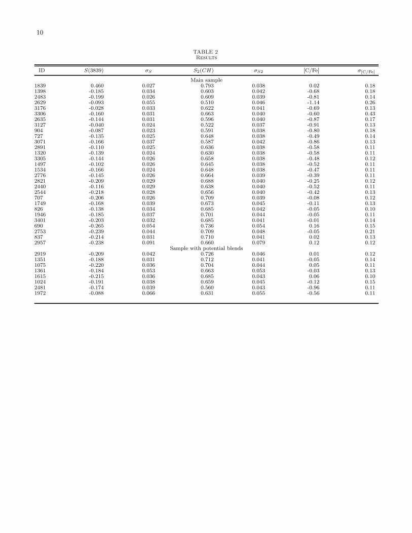
TABLE 2Results

ID S(3839) σS S2(CH) σS2 [C/Fe] σ[C/Fe]

Main sample1839 0.460 0.027 0.793 0.038 0.02 0.181398 -0.185 0.034 0.603 0.042 -0.68 0.182483 -0.199 0.026 0.609 0.039 -0.81 0.142629 -0.093 0.055 0.510 0.046 -1.14 0.263176 -0.028 0.033 0.622 0.041 -0.69 0.133306 -0.160 0.031 0.663 0.040 -0.60 0.432635 -0.144 0.031 0.596 0.040 -0.87 0.173127 -0.040 0.024 0.522 0.037 -0.91 0.13904 -0.087 0.023 0.591 0.038 -0.80 0.18727 -0.135 0.025 0.648 0.038 -0.49 0.143071 -0.166 0.037 0.587 0.042 -0.86 0.132891 -0.110 0.025 0.636 0.038 -0.58 0.111320 -0.139 0.024 0.630 0.038 -0.58 0.113305 -0.144 0.026 0.658 0.038 -0.48 0.121497 -0.102 0.026 0.645 0.038 -0.52 0.111534 -0.166 0.024 0.648 0.038 -0.47 0.112776 -0.145 0.026 0.664 0.039 -0.39 0.112821 -0.209 0.029 0.688 0.040 -0.25 0.122440 -0.116 0.029 0.638 0.040 -0.52 0.112544 -0.218 0.028 0.656 0.040 -0.42 0.13707 -0.206 0.026 0.709 0.039 -0.08 0.121749 -0.168 0.039 0.673 0.045 -0.11 0.13826 -0.138 0.034 0.685 0.042 -0.05 0.101946 -0.185 0.037 0.701 0.044 -0.05 0.113401 -0.203 0.032 0.685 0.041 -0.01 0.14690 -0.265 0.054 0.736 0.054 0.16 0.152753 -0.239 0.044 0.709 0.048 -0.05 0.21837 -0.214 0.031 0.710 0.041 0.02 0.132957 -0.238 0.091 0.660 0.079 0.12 0.12

Sample with potential blends2919 -0.209 0.042 0.726 0.046 0.01 0.121351 -0.188 0.031 0.712 0.041 -0.05 0.141075 -0.220 0.036 0.704 0.044 0.05 0.111361 -0.184 0.053 0.663 0.053 -0.03 0.131615 -0.215 0.036 0.685 0.043 0.06 0.101024 -0.191 0.038 0.659 0.045 -0.12 0.152481 -0.174 0.039 0.560 0.043 -0.96 0.111972 -0.088 0.066 0.631 0.055 -0.56 0.11