Journal of Constructional Steel Research 90 (2013) 60–71

Contents lists available at ScienceDirect

Journal of Constructional Steel Research

A novel formulation of the flexural overstrength factor for steel beams

Esra Mete Güneyisi a,⁎, Mario D'Aniello b, Raffaele Landolfo b, Kasım Mermerdaş c

a Department of Civil Engineering, Gaziantep University, Gaziantep, Turkeyb Department of Structures for Engineering and Architecture, University of Naples “Federico II”, Naples, Italyc Department of Civil Engineering, Hasan Kalyoncu University, Gaziantep, Turkey

⁎ Corresponding author. Tel.: +90 342 3172423; fax: +E-mail address: eguneyisi@gantep.edu.tr (E.M. Güney

0143-974X/$ – see front matter © 2013 Elsevier Ltd. All rhttp://dx.doi.org/10.1016/j.jcsr.2013.07.022

a b s t r a c t

a r t i c l e i n f o

Article history:Received 23 January 2013Accepted 16 July 2013Available online 19 August 2013

Keywords:Analytical modellingFlexural overstrengthExperimental databaseSteel beamsSteel structures

The ductile design of steel structures is directly influenced by the flexural behaviour of steel beams, which shouldbe sufficient to allow plastic hinges to rotate until the collapsemechanism is completely developed. To guaranteethe achievement of such a performance, the beam flexural overstrength must be quantified to appropriatelyapply capacity design principles. To this aim, analytical formulations to predict the flexural overstrength factor(s) of steel beams with a wide range of cross-section typologies (I and H sections, square and rectangular hollowsections) were developed based on gene expression programming (GEP). An experimental database was gath-ered from the available literature and processed to obtain the training and testing databases for the derivationof the closed-form solution through GEP. The independent variables used for the development of the predictionmodels were the geometric properties of the sections, the mechanical properties of the material, and the shearlength of the steel beams. The predictions of the proposed GEP-based models were compared with the resultsobtainedusing the existing analytical equations proposed in the current literature. Comparative analysis revealedthat the proposed formulation provides a more accurate prediction of beam overstrength.

© 2013 Elsevier Ltd. All rights reserved.

1. Introduction

The flexural behaviour of steel beams plays a key role in the structur-al performance of steel moment-resisting frames. The main responseparameters governing the beam behaviour are the rotation capacityand the flexural ultimate resistance [1,2]. The former is the source ofthe local ductility supply needed to achieve a global dissipative structur-al behaviour, whereas the latter governs the flexural overstrength,whichmust be accurately known to appropriately apply capacity designprinciples, as currently implemented in all modern seismic codes. Thisdesign philosophy leads to the formation of a ductile mechanism inthe structures to dissipate the seismic input energy through plastic de-formations within specific parts (namely, members and/or connec-tions) of the structure itself [3]. Additionally, it may be necessary todesign the main structural elements along a similar design approachunder non-seismic conditions, such as in the case of robustness underexceptional loading, where it is crucial to enhance the local resistanceof principal members to prevent progressive collapse [4]. Hence, bothunder seismic conditions and in the case of exceptional loading, it is fun-damental to guarantee that the structural elements connected to ductileparts are designed to resist the maximum strength experienced by thelatter. Thus, an effective estimation of the level of hardening developingin such elements prior to strength degradation is essential at the designstage for the safe application of capacity design rules [5,6].

90 342 3601107.isi).

ights reserved.

To this end, several studies have been carried out to derive analyticalformulations for the rotation capacity and flexural overstrength of thestructural steel members [1,2,7–15]. In particular, some studies haveused computational tools (namely, finite element analysis) or have de-veloped computational aids. For example, in the study ofWilkinson andHancock [15], finite element analysis was applied to cold-formed rect-angular hollow section (RHS) beams to predict the rotation capacity ofclass 1 (plastic) and 2 (compact) beams. Gioncu et al. [9] andAnastasiadis et al. [10] developed a computer programme (DUCTROT-M) todetermineboth theflexural strength and the available rotation ca-pacity of wide-flange beams.

Recently, novel approaches based on soft computing have beenemployed to address the analysis and design of steel structures, thusborrowing from artificial intelligence philosophies widely used tosolve sophisticated engineering problems in the past [16–29]. For exam-ple, in the study of Saka [16], a genetic-algorithm-based optimum de-sign is presented for pitched-roof steel portal frames with haunchesfor the rafters at the eaves. Gholizadeh et al. [17] used finite element(FE) and soft computing techniques, namely, back-propagation (BP)neural network and adaptive neuro-fuzzy inference system (ANFIS)methods, to propose models for the estimation of the critical bucklingload of the web posts of castellated steel beams. Fonseca et al. [18]utilised neural networks to forecast steel beam patch load resistance,comparing the results with preceding models and existing design for-mulae. They concluded that the networks' percentage errors relativeto the experimental results confirm the possibility of using the unifiedmethodology to generate new data accurately. In the study of Gandomiet al. [19], an alternative approach for predicting the flexural resistance

M /Mp

θ /θ p

1

1 θ u /θ p

Mmax /Mp

R

s

Fig. 1. Generalised moment–rotation curve for a steel beam [1].

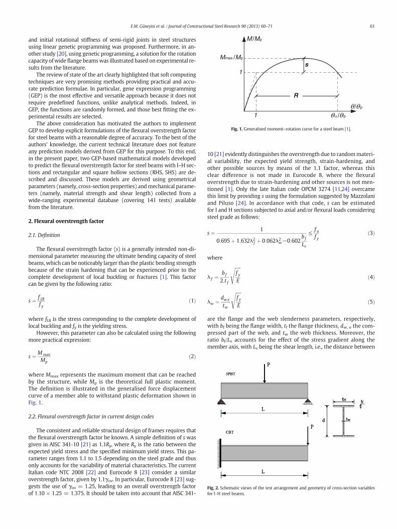
Fig. 2. Schematic views of the test arrangement and geometry of cross-section variablesfor I–H steel beams.

61E.M. Güneyisi et al. / Journal of Constructional Steel Research 90 (2013) 60–71

and initial rotational stiffness of semi-rigid joints in steel structuresusing linear genetic programming was proposed. Furthermore, in an-other study [20], using genetic programming, a solution for the rotationcapacity ofwide flange beamswas illustrated based on experimental re-sults from the literature.

The review of state of the art clearly highlighted that soft computingtechniques are very promising methods providing practical and accu-rate prediction formulae. In particular, gene expression programming(GEP) is the most effective and versatile approach because it does notrequire predefined functions, unlike analytical methods. Indeed, inGEP, the functions are randomly formed, and those best fitting the ex-perimental results are selected.

The above consideration has motivated the authors to implementGEP to develop explicit formulations of the flexural overstrength factorfor steel beams with a reasonable degree of accuracy. To the best of theauthors' knowledge, the current technical literature does not featureany prediction models derived from GEP for this purpose. To this end,in the present paper, two GEP-based mathematical models developedto predict the flexural overstrength factor for steel beams with I–H sec-tions and rectangular and square hollow sections (RHS, SHS) are de-scribed and discussed. These models are derived using geometricalparameters (namely, cross-section properties) andmechanical parame-ters (namely, material strength and shear length) collected from awide-ranging experimental database (covering 141 tests) availablefrom the literature.

2. Flexural overstrength factor

2.1. Definition

The flexural overstrength factor (s) is a generally intended non-di-mensional parameter measuring the ultimate bending capacity of steelbeams,which can be noticeably larger than the plastic bending strengthbecause of the strain hardening that can be experienced prior to thecomplete development of local buckling or fractures [1]. This factorcan be given by the following ratio:

s ¼ f LBf y

ð1Þ

where fLB is the stress corresponding to the complete development oflocal buckling and fy is the yielding stress.

However, this parameter can also be calculated using the followingmore practical expression:

s ¼ Mmax

Mpð2Þ

where Mmax represents the maximum moment that can be reachedby the structure, while Mp is the theoretical full plastic moment.The definition is illustrated in the generalised force displacementcurve of a member able to withstand plastic deformation shown inFig. 1.

2.2. Flexural overstrength factor in current design codes

The consistent and reliable structural design of frames requires thatthe flexural overstrength factor be known. A simple definition of s wasgiven in AISC 341-10 [21] as 1.1Ry, where Ry is the ratio between theexpected yield stress and the specified minimum yield stress. This pa-rameter ranges from 1.1 to 1.5 depending on the steel grade and thusonly accounts for the variability of material characteristics. The currentItalian code NTC 2008 [22] and Eurocode 8 [23] consider a similaroverstrength factor, given by 1.1γov. In particular, Eurocode 8 [23] sug-gests the use of γov = 1.25, leading to an overall overstrength factorof 1.10 × 1.25 = 1.375. It should be taken into account that AISC 341-

10 [21] evidently distinguishes the overstrength due to randommateri-al variability, the expected yield strength, strain-hardening, andother possible sources by means of the 1.1 factor, whereas thisclear difference is not made in Eurocode 8, where the flexuraloverstrength due to strain-hardening and other sources is not men-tioned [1]. Only the late Italian code OPCM 3274 [11,24] overcamethis limit by providing s using the formulation suggested by Mazzolaniand Piluso [24]. In accordance with that code, s can be estimatedfor I and H sections subjected to axial and/or flexural loads consideringsteel grade as follows:

s ¼ 1

0:695þ 1:632λ2f þ 0:062λ2

w−0:602bf

Lv

≤ f uf y

ð3Þ

where

λ f ¼bf

2:t f

ffiffiffiffiffif yE

sð4Þ

λw ¼ dw;e

tw

ffiffiffiffiffif yE

sð5Þ

are the flange and the web slenderness parameters, respectively,with bf being the flange width, tf the flange thickness, dw, e the com-pressed part of the web, and tw the web thickness. Moreover, theratio bf/Lv accounts for the effect of the stress gradient along themember axis, with Lv being the shear length, i.e., the distance between

Fig. 3. Schematic views of the test arrangement and geometry of cross-section variablesfor RHS–SHS steel beams.

62 E.M. Güneyisi et al. / Journal of Constructional Steel Research 90 (2013) 60–71

the plastic hinge and the point of zero moment. The compressed part ofthe web, i.e., the effective compressed web, can be computed accordingto [25] as

dw;e ¼12

1þ AAw

ρ� �

dw ð6Þ

where A is the section area, Aw is the web area, dw is theweb depth, andρ is the non-dimensional axial load, i.e., the ratio between the axial loadand the squash load.

2.3. Review of the existing analytical formulations

2.3.1. Flexural overstrength factor for I and H profilesTo estimate the overstrength factor of the steel beams in relation

to the cross-sectional dimensions and material characteristics, vari-ous relations have been proposed in the literature [1,2,11,25–27].Kato [25,26] proposed empirical equations to estimate the flexuraloverstrength based on the results of 68 tests conducted on “stub-column”specimenswith different steel grades and local (flange andweb) slender-ness parameters. The normalised overstrength swas obtained bymultiple

Table 1Summary of the experimental database for the I–H and RHS–SHS steel beams.

No. Authors Test no. Profile ty

1 Lukey and Adams (1969) [35] 12 I and H h2 Climenhaga (1970) [36] 10 I welded3 Grubb and Carskaddan (1979,1981) [37,38] 7 I welded4 Kemp (1985) [39] 14 I and H w5 Schilling (1988,1990) [40,41] 3 I welded6 Wargsjö (1991) [42] 10 I welded7 Dahl et al. (1992) [43] 6 I welded8 Boeraeve and Lognard (1993) [44] 5 I and H h9 Suzuki et al. (1994) [45] 6 I welded10 Landolfo et al. (2011) [1,46] 3 I and H h11 Wilkinson (1999) [29] 44 Cold-for12 Zhou and Young (2005) [47] 15 Cold-for13 Landolfo et al. (2011) [1,46] 6 Cold-for

a MCS = mild carbon steel.b HSS = high-strength steel.c 3PBT = 3-point bending test.d 4PBT = 4-point bending test.e CBT = cantilever bending test.

regression analysis as function of the flange andweb slenderness for eachgrade of steel, whose expression is given by the following:

1s¼ 0:6003þ 1:600

α fþ 0:1535

αwð7Þ

where

α f ¼Ef y

t fb f =2

!2

ð8Þ

is the slenderness parameter of the flange and

αw ¼ Ef y

twdw

� �2ð9Þ

is the slenderness parameter of theweb, dw is theweb height, tw is theweb thickness, fy is the yield strength, and E is themodulus of elasticity ofsteel.

Brescia [2] proposed a novel expression of s, recalibrating the coeffi-cients of the formulation developed by [24] and adopted by OPCM3274[11,24]. From the multiple regression of a limited set of experimentaldata, she derived the following expression:

1s¼ 0:349þ 0:827λ2

f þ 0:03λ2w−0:239

bf

Lv−0:045

EEh

þ 0:263εhεy

: ð10Þ

Moreover, considering the averagemechanical properties of Europeanmild carbon steel, Eq. (10) can be specialised as follows [2]:

1s¼ 1:323þ 0:827λ2

f þ 0:03λ2w−0:239

bf

Lvð11Þ

More recently, in a study by D'Aniello et al. [1], another empiricalequation for predicting swas derived bymultiple linear regression anal-ysis using a wider database of experimental tests, as follows:

1s¼ 1:71þ 0:167λ2

f þ 0:006λ2w−0:134

bf

Lv−0:007

EEh

−0:0053εhεy

: ð12Þ

2.3.2. Flexural overstrength factor for RHS and SHS profilesA number of predictive equations for evaluating flexural overstrength

of steel beams with RHS and SHS profiles are available in the literature

pe Steel grade Test setup Loading history

ot-rolled MCSa 3PBTc MonotonicMCS 3PBT MonotonicHSSb 3PBT Monotonic

elded + hot-rolled MCS 3PBT MonotonicHSS 3PBT MonotonicHSS 3PBT MonotonicHSS 3PBT Monotonic

ot-rolled MCS 3PBT MonotonicMCS + HSS 3PBT Monotonic

ot rolled MCS CBTe Monotonicmed RHS + SHS MCS 4PBTd Monotonicmed RHS + SHS MCS + HSS 4PBT Monotonicmed RHS + SHS MCS CBT Monotonic

Table 2Input and output database of training and test sets for I–H steel beams.

Ref no. Data no. bf d tf tw Lv fy, flange fy, web E/Eh εh/εy s

[35] 1 203.5 256.7 10.8 7.65 1740 283 308 42.8 11 1.382 176 256.7 10.8 7.65 1473 283 308 42.8 11 1.413 102.6 201.86 5.28 4.45 777 371 395 48.2 9.8 1.114 73.9 201.86 5.28 4.45 518 371 395 48.2 9.8 1.155 86.1 201.86 5.28 4.45 627 371 395 48.2 9.8 1.136 94 201.86 5.28 4.45 698 371 395 48.2 9.8 1.057 96.8 201.82 5.26 4.45 724 371 395 48.2 9.8 1.048 101.9 251.72 5.26 4.6 686 371 350 48.2 9.8 1.119 73.7 251.72 5.26 4.6 480 371 350 48.2 9.8 1.26

10 85.9 251.72 5.26 4.6 584 371 350 48.2 9.8 1.1611 93.5 251.72 5.26 4.6 648 371 350 48.2 9.8 1.1212 88.9 251.72 5.26 4.6 640 371 350 48.2 9.8 1.14

[36] 13 135 201 8 5.7 1956 315 344 48.2 9.8 1.0914 134 204 9.5 6 1956 293 310 42.8 11 1.2215 104 305.8 6.9 6 1956 357 412 48.2 9.8 0.8916 128 352 8 6 1956 324 363 48.2 9.8 0.8617 141 398.2 7.6 6.2 1956 303 379 42.8 11 0.9218 135 201 8 5.7 1346 315 344 48.2 9.8 1.0619 134 204 9.5 6 1346 293 310 42.8 11 1.2620 104 305.8 6.9 6 1346 357 412 48.2 9.8 0.9721 128 352 8 6 1346 324 363 48.2 9.8 0.9222 105 308.6 10.3 6.2 1346 319 384 48.2 9.8 0.97

[37,38] 23 156 406.4 9.7 6.7 914 383 345 48.2 9.8 1.0424 156 406.4 9.7 6.7 1829 383 345 48.2 9.8 1.0025 156 406.4 9.7 6.7 2743 383 345 48.2 9.8 0.9626 157 308.4 11.2 8.3 1219 370 337 48.2 9.8 1.3127 150 374.4 11.2 8.4 1524 370 337 48.2 9.8 1.1528 130 404.4 11.2 8.4 1524 370 337 48.2 9.8 1.1029 158 407.4 11.2 8.4 1524 370 337 48.2 9.8 1.08

[39] 30 150 217.8 8.09 6.65 1830 340 358 48.2 9.8 1.1231 145 217.4 10.57 6.82 1830 285 329 42.8 11 1.1432 106 273.9 7.05 5.85 1830 332 388 48.2 9.8 1.0333 149 217.9 8.56 6.78 915 340 358 48.2 9.8 1.2734 149 217.1 8.44 6.78 915 294 300 42.8 11 1.2235 140 209.5 10.77 6.76 915 288 329 42.8 11 1.2736 145 366.3 8.33 5.96 1830 375 403 48.2 9.8 1.0137 154 120.3 9.83 7.44 1830 313 300 48.2 9.8 1.2238 146 217.9 9.03 6.35 1830 340 358 48.2 9.8 1.0939 105 282.2 6.92 5.82 1830 332 388 48.2 9.8 1.0040 104 277.5 6.76 5.59 2179 317 351 48.2 9.8 1.0541 145.54 402.2 11.11 6.84 1830 285 329 42.8 11 1.1142 180 210 8.05 6.11 1830 332 326 48.2 9.8 1.1843 180 210 8 6 1816 332 326 48.2 9.8 1.26

[40,41] 44 127 611 7 5.3 1067 410 450 48.2 9.8 0.6845 229 622 12.5 5.3 1981 401 450 48.2 9.8 0.8146 311 945.4 15.7 5.3 2895.5 342 450 48.2 9.8 0.89

[42] 47 131 500.8 9.9 4 1910 370 335 48.2 9.8 0.9148 130 501.8 9.9 4 2860 370 335 48.2 9.8 0.8949 131 457 10 4 1760 370 335 48.2 9.8 0.9250 131 458.8 9.9 4 2640 370 335 48.2 9.8 0.9551 132 414.6 9.8 4 1610 370 335 48.2 9.8 0.9452 130 422 10 4 2400 370 335 48.2 9.8 0.9253 131 379.8 9.9 4 1460 370 335 48.2 9.8 0.9954 131 379.8 9.9 4 2160 370 335 48.2 9.8 0.9755 131 336 10 4 1310 370 335 48.2 9.8 1.0256 131 339.6 9.8 3.9 1920 370 335 48.2 9.8 0.98

[43] 57 202 200 15 9.5 1500 428 456 48.2 9.8 1.3658 202 200 15 9.5 1500 428 456 48.2 9.8 1.3059 280 280 18 10 1500 982 984 48.2 9.8 1.0960 280 280 18 10 1500 864 813 48.2 9.8 1.0661 280 280 18 10 1500 468 536 48.2 9.8 1.0662 280 280 18 10 1500 278 323 48.2 9.8 1.24

[44] 63 200.7 183.3 14.1 8.8 1500 303 342 42.8 11 1.1464 200.2 183.3 14.7 9.5 1500 375 421 48.2 9.8 1.1565 201.5 184.6 15.1 9.5 1500 445 462 48.2 9.8 1.1666 200.4 185.8 14.6 9.6 1500 261 291 37.5 12.3 1.1367 199.9 189.3 14.9 9.4 1500 409 426 48.2 9.8 1.15

[45] 68 150 132 9 6 600 291 340 42.8 11 1.2569 150 132 9 6 900 291 340 42.8 11 1.2370 150 132 9 6 600 526 509 48.2 9.8 1.2671 150 132 9 6 600 527 340 48.2 9.8 1.2072 150 132 9 6 600 291 509 42.8 11 1.1573 150 132 9 6 900 291 686 42.8 11 1.14

(continued on next page)

63E.M. Güneyisi et al. / Journal of Constructional Steel Research 90 (2013) 60–71

Table 3Input and output database of training and test sets for RHS–SHS steel beams.

Ref no. Data no. b d t r Lv fy E/Eh εh/εy s

[29] 1 50.25 151.04 4.92 9.9 450 441 48.2 9.8 1.232 50.41 150.92 4.9 10.7 450 441 48.2 9.8 1.173 50.27 150.43 3.92 6.8 450 457 48.2 9.8 1.274 50.4 150.44 3.87 7.3 450 457 48.2 9.8 1.195 50.11 150.42 3.89 7.3 450 457 48.2 9.8 1.246 50.16 150.21 3.89 5.4 450 423 48.2 9.8 1.177 50.22 150.47 2.97 5.9 450 444 48.2 9.8 1.158 50.01 150.79 2.95 5.8 450 444 48.2 9.8 1.169 50.34 150.8 2.96 5.7 450 444 48.2 9.8 1.13

10 50.15 150.43 2.6 4.6 450 446 48.2 9.8 1.0211 50.41 150.39 2.57 4.6 450 446 48.2 9.8 1.0012 50.23 150.4 2.59 4.8 450 446 48.2 9.8 1.1013 50.4 150.31 2.64 5.3 450 440 48.2 9.8 1.1114 50.64 150.65 2.25 4.6 450 444 48.2 9.8 0.9815 50.57 150.51 2.28 4.2 450 444 48.2 9.8 1.0116 50.7 150.37 2.26 4.8 450 444 48.2 9.8 0.9817 50.7 100.45 2.06 3.8 450 449 48.2 9.8 1.0718 50.55 100.49 2.07 3.9 450 449 48.2 9.8 1.0119 50.24 100.46 2.04 4.7 450 449 48.2 9.8 1.0720 50.22 100.45 2.04 3.4 450 423 48.2 9.8 1.0821 50.1 75.48 1.94 4.4 400 411 48.2 9.8 1.0422 50.31 75.63 1.95 4.4 400 411 48.2 9.8 1.0223 25.28 75.31 1.98 3.7 400 457 48.2 9.8 1.1124 25.23 75.33 1.95 4 400 457 48.2 9.8 1.1325 25.12 75.24 1.54 3.1 400 439 48.2 9.8 1.0826 25.2 74.9 1.54 3.4 400 439 48.2 9.8 1.1327 25.08 74.98 1.56 3.9 400 439 48.2 9.8 1.0928 25.12 75.27 1.55 3.4 400 422 48.2 9.8 1.0329 25.25 75.19 1.56 3.4 400 422 48.2 9.8 1.0030 50.13 150.46 3 6.2 450 370 48.2 9.8 1.2131 50.19 150.5 2.96 6.5 450 370 48.2 9.8 1.1532 50.51 150.45 3 6.8 450 382 48.2 9.8 1.1833 50.51 150.38 3 6.3 450 382 48.2 9.8 1.2134 50.43 100.91 2.06 3.6 450 400 48.2 9.8 1.0035 50.52 100.83 2.05 3.8 450 400 48.2 9.8 1.0036 75.84 125.56 2.92 6.6 450 397 48.2 9.8 1.0337 75.74 125.4 2.93 6.9 450 397 48.2 9.8 1.0438 75.56 125.4 2.91 7.1 450 397 48.2 9.8 1.0339 75.1 125.4 2.53 3.9 450 374 48.2 9.8 1.0640 100.27 100.43 2.88 5.2 450 445 48.2 9.8 1.0241 100.33 100.53 2.91 5 450 445 48.2 9.8 0.9542 100.25 100.53 2.86 5.2 450 445 48.2 9.8 1.0343 50.21 150.32 3.9 7.9 450 349 48.2 9.8 1.2844 50.57 150.39 3.85 7.5 450 410 48.2 9.8 1.19

[47] 45 40.1 40.1 1.96 2 480.7 447 48.2 9.8 1.2946 40 40.1 3.88 4 480.3 565 48.2 9.8 1.3147 80.5 80.4 1.91 4 480.7 398 48.2 9.8 0.9848 79.9 79.8 4.77 7.5 481 448 48.2 9.8 1.4949 49.8 99.9 1.97 2 480 320 48.2 9.8 1.5150 49.6 99.7 3.88 4 479.7 378 48.2 9.8 1.7151 59.9 120.2 1.84 2.5 480.7 361 48.2 9.8 1.1452 59.7 120 3.89 5.5 480.7 392 48.2 9.8 1.8053 40.2 40 1.94 2 414.3 707 48.2 9.8 1.2154 50.1 50.3 1.54 1.5 414 622 48.2 9.8 1.0555 150.6 150.7 2.78 4.8 546.7 448 48.2 9.8 0.7856 150.7 150.5 5.87 6 550 497 48.2 9.8 1.2357 80.5 140.3 3.09 6.5 480 486 48.2 9.8 1.1958 80.9 160.6 2.9 6 480 536 48.2 9.8 1.0759 109.1 197.7 4 8.5 548 503 48.2 9.8 1.07

[1,46] 60 100 150 5 10 1875 275 42.6 11 1.2961 80 160 4 8 1875 275 42.6 11 1.2562 100 250 10 20 1875 275 42.6 11 1.4463 160 160 6.3 12.6 1875 355 48.2 9.8 1.0564 200 200 10 20 1875 355 48.2 9.8 1.2865 250 250 8 16 1875 355 48.2 9.8 1.14

Table 2 (continued)

Ref no. Data no. bf d tf tw Lv fy, flange fy, web E/Eh εh/εy s

[1,46] 74 160 152 9 6 1875 275 275 42.8 11 1.3075 240 240 17 10 1875 275 275 42.8 11 1.3676 150 300 10.7 7.1 1875 275 275 42.8 11 1.22

64 E.M. Güneyisi et al. / Journal of Constructional Steel Research 90 (2013) 60–71

[1,2,25,26]. For example, Kato [25,26] proposed a relationship generalisedfor cold-formed SHS, given by the following:

1s¼ 0:778þ 0:13

αð13Þ

where

α ¼ Ef y

tb

� �2ð14Þ

is the slenderness parameter for the SHS section, with b being the widthof the edge in compression and t being the corresponding thickness.

Brescia [2] proposed a formulation for s obtained bymulti-linear re-gression analysis of the experimental data obtained from tests carriedout by Wilkinson [29] on cold-formed profiles. Thus, the following ex-pressions were provided:

1s¼ 0:711þ 0:09λ2

f þ 0:318λ2w−0:189

bf

Lvfor SHS beams ð15Þ

1s¼ 2:7þ 0:62λ2

f þ 0:0206λ2w−2:11

bf

Lvfor RHS beams: ð16Þ

More recently, based on a wider experimental database, D'Anielloet al. [1] proposed a unique equation to estimate the flexuraloverstrength factor for RHS and SHS steel beams, given as follows:

1s¼ 0:014þ 0:294λ2

f þ 0:094λ2w−0:713

bf

Lvþ 0:017

EEh

: ð17Þ

3. Overview of genetic programming

A genetic algorithm (GA) is a search technique used in computing tofind precise or approximate solutions to optimisation or search prob-lems. GAs are a particular class of evolutionary computation and canbe categorised as global search heuristics. The techniques used by GAare inspired by evolutionary biology, including inheritance, mutation,selection, and crossover (recombination).

Genetic programming (GP) is essentially the application of geneticalgorithms to computer programmes [30]. GP has been applied success-fully to solve discrete, non-differentiable, combinatory, and generalnonlinear engineering optimisation problems [31]. It is an evolutionaryalgorithm-based methodology inspired by biological evolution used todevelop a computer programme that performs a user-defined task.Therefore, it is a machine-learning technique used to create a popula-tion of computer programmes according to a fitness landscape deter-mined by a programme's ability to perform a given computationaltask. Similar to GA, the GP only needs the problem to be defined asinput. Next, the programme searches for a solution in a problem-independent manner [30,32].

Gene expression programming (GEP), introduced by Ferreira [33],can be considered a natural development of genetic algorithms and ge-netic programming. In detail, GEP evolves computer programmes of dif-ferent sizes and shapes encoded in fixed-length linear chromosomes. AGEP algorithm begins with a random generation of the fixed-lengthchromosomes of each individual in the initial population. Next, the

Table 4Statistics for the experimental data for I–H steel beams.

bf d tf tw Lv fy, flange fy, web E/Eh εh/εy s

a) Training dataNo. of data 57 57 57 57 57 57 57 57 57 57Mean 145.89 286.65 9.84 6.39 2905.65 374.28 380.16 46.97 10.08 1.09Standard deviation 44.34 111.85 3.22 1.85 1098.23 118.88 112.16 2.50 0.56 0.14COV 0.30 0.39 0.33 0.29 0.38 0.32 0.30 0.05 0.06 0.13Min. value 73.70 120.30 5.26 3.90 960 261 275 37.50 9.80 0.68Max. value 280.00 622.00 18.00 10.00 5486.00 982.00 984.00 48.20 12.30 1.36

b) Test dataNo. of data 19 19 19 19 19 19 19 19 19 19Mean 169.64 301.45 10.11 6.32 3166.26 337.47 383.05 46.49 10.18 1.12Standard deviation 62.24 189.84 3.82 1.81 1318.66 50.25 99.43 2.58 0.57 0.15COV 0.37 0.63 0.38 0.29 0.42 0.15 0.26 0.06 0.06 0.13Min. value 88.9 132.0 5.3 4.0 1200.0 275.0 275.0 42.8 9.8 0.9Max. value 311 945 18 10 5791 468 686 48 11 1

Table 5Statistics for the experimental data for RHS–SHS steel beams.

bf d t r Lv fy E/Eh εh/εy s

a) Training dataNo. of data 49 49 49 49 49 49 49 49 49Mean 63.43 123.94 2.96 5.68 532.39 420.82 48.09 9.82 1.13Standard deviation 41.64 37.08 1.58 3.18 347.26 39.73 0.80 0.17 0.17COV 0.66 0.30 0.53 0.56 0.65 0.09 0.02 0.02 0.15Min. value 25.08 74.90 1.54 2.00 400.00 320.00 42.60 9.80 0.95Max. value 250.00 250.00 10.00 20.00 1875.00 536.00 48.20 11.00 1.80

b) Test dataNo. of data 16 16 16 16 16 16 16 16 16Mean 74.57 128.89 3.96 6.94 736.85 445.38 47.15 10.03 1.19Standard deviation 37.61 61.26 2.03 4.47 566.25 121.14 2.26 0.48 0.16COV 0.50 0.48 0.51 0.64 0.77 0.27 0.05 0.05 0.13Min. value 40 40 1.54 1.50 414 275 42.60 9.80 0.78Max. value 150.70 250 10 20 1875 707 48.20 11.00 1.44

65E.M. Güneyisi et al. / Journal of Constructional Steel Research 90 (2013) 60–71

chromosomes are expressed, and the fitness of each individual is evalu-ated based on the quality of the solution it represents [34]. Based onGEP, novel formulations for the flexural overstrength of steel beamsare proposed hereinafter.

Table 6GEP parameters used for the proposed models.

Parameter s for I–H profiles s ′ for RHS–SHS profiles

P1 Function set +,−, *, /, √, ^,ln, exp, sin, cos, tan,

arctan

+,−, *, /, √, ^,ln, exp, sin, cos, tan,

arctanP2 Number of generation 492,531 478,574P3 Chromosomes 30 30P4 Head size 10 10P5 Linking function Addition AdditionP6 Number of genes 8 8P7 Mutation rate 0.044 0.044P8 Inversion rate 0.1 0.1P9 One-point recombination rate 0.3 0.3P10 Two-point recombination rate 0.3 0.3P11 Gene recombination rate 0.1 0.1P12 Gene transposition rate 0.1 0.1

4. Proposed GEP formulation

New formulations of the flexural overstrength factor (s) for I–H andRHS–SHS steel beams were derived using a set of experimental dataavailable in the technical literature [1,35–47]. The examined test config-urations, accounting for different load patterns (namely, bending mo-ment distribution) are depicted in Figs. 2 and 3. The data sourcespresented in Table 1 contain precisely selected data samples to ensurea wide range of cross-section typologies under monotonic loadingwith different local slenderness ratios. The experimental data are re-ported in Tables 2 and 3 for I–H and RHS–SHS beams, respectively. Allof the data samples were ordered to create a consistent sequence ofthe inputs to be used for the derivation of the models. The input nodesinclude the geometric properties of the section, the mechanical proper-ties of the material, and the shear length of the steel beams. Thus, nineand eight input parameters were utilised for the development of GEPmodels for the I–H and RHS–SHS profiles, respectively.

The model generated for I–H sections consists of the following pa-rameters: bf (width of flange), d (depth of section), tf (thickness offlange), tw (thickness of web), Lv (shear length), fy, flange (yield stress offlange), fy, web (yield stress of web), E/Eh (ratio of themodulus of elastic-ity of steel to the hardeningmodulus), and εh/εy (ratio of the strain cor-responding to the beginning of hardening to the yield strain) (Table 2).

The GEP model for the RHS–SHS profiles included the followinginput parameters: b (width of section), d (depth of section), t (wallthickness of section), r (inside corner radius), Lv (shear length), fy(yield stress), E/Eh, and εh/εy (Table 3).

The development of a genetic-programming-based mathematicalformulation is achieved using the training data containing input andoutput variables. Moreover, to examine and test the performance ofthe generated model, an optional data set containing the same numberand sequence of input and output variables is used. Therefore, in thecurrent study, two ensembles of available experimental data (one forI–H and one for RHS–SHS beams) were arbitrarily divided into twoparts to obtain the training and testing databases. Approximately 1/4

Fig. 4. GEP model expression tree for I–H steel beams.

66 E.M. Güneyisi et al. / Journal of Constructional Steel Research 90 (2013) 60–71

of the total data samples were used as the test database, while therest were used as the training database, as shown in Tables 2 and 3.Thus, 57 and 49 data samples were used as the training data for I–H and RHS–SHS profiles, respectively, and the testing databasecontained 19 data samples for the former and 16 for the latter. Thestatistical analyses of the data presented in Tables 2 and 3 aresummarised in Tables 4 and 5, respectively. As can be observed inTables 4 and 5, the statistics for both the training and testing setsare in good agreement, meaning that both of them represent almostidentical populations.

GeneXproTools 4.0 software was utilised for the derivation of themathematical model. The GEP parameters used for the derivation ofthe mathematical models are given in Table 6. As seen from Table 6, toprovide an accurate model, various mathematical operations wereused. Several modifications of the GEP parameters have been made toobtain an optimummodelwith the bestfitness. However, trigonometricoperations in combination with exponential functions were predomi-nantly included in the GEP models presented in this study.

The correlation coefficient (R) (Eq. (18)) describes the fit of theGEP's output variable approximation curve to the actual test data output

Fig. 5. Evaluation of the experimental and predicted flexural overstrength factors for I–Hsteel beams: A) training set and B) test set.

67E.M. Güneyisi et al. / Journal of Constructional Steel Research 90 (2013) 60–71

variable curve. Higher R coefficients indicate amodelwith better outputapproximation capability.

R ¼X

mi−m′ð Þ pi−p′ð ÞffiffiffiffiffiffiffiffiffiffiffiffiffiffiffiffiffiffiffiffiffiffiffiffiffiffiffiffiffiffiffiffiffiffiffiffiffiffiffiffiffiffiffiffiffiffiffiffiffiffiffiffiffiffiffiXmi−m′ð Þ2

Xpi−p′ð Þ2

q ð18Þ

wherem′ and p′ are themeans of the measured (mi) and predicted (pi)values, respectively.

4.1. GEP formulation for I and H beams

The prediction model for I–H sections derived from GEP ispresented in Eq. (19). The models developed by the software in itsnative language can be automatically parsed into visually appealingexpression trees, permitting a quicker and more complete compre-hension of their mathematical/logical intricacies. Fig. 4 demon-strates the expression tree for the terms used in the formulation ofthe GEP model. In the expression tree given in Fig. 4, each of thefirst seven sub-parts of the tree contains various input variables.However, Sub-ET 8 has no independent variable and is instead thecosine of a real number. Therefore, S8 in the mathematical modelwas taken as a constant input, −0.51304.

The performance of the proposed GEP prediction model inEq. (19) was graphically depicted in Fig. 5 for both the training andtesting data sets. The variations of the predicted and experimentaldata are strongly correlated, with correlation coefficients of 0.928and 0.929 for the training and testing databases, respectively. More-over, the closeness of the values of the correlation coefficients may

also be considered as evidence for the consistency and good fitnessof the proposed model.

s ¼ s1 þ s2 þ s3 þ s4 þ s5 þ s6 þ s7 þ s8 ð19Þ

s1 ¼ sin

ffiffiffiffiffiffiffiffiffiffiffiffiffiffiffiffiffiffiffiffiffiffiffiffiffiffiffiffiffiffiffiffiffiffiffiffiffiffiffiffiffiffiffiffiffiffiffiffiffiffiffiffiffiffiffiffiffiffiffiffiffiffiffiffiffiffiffiffiffisin

d2 þ 5:179657d1−d7

� ��

ffiffiffiffiffiffiffied8

4p� �

4

s" #ð19aÞ

s2 ¼ cos sin cos tan tan tan cosd4 þ d8=d7ð Þð Þð Þð Þð Þð Þ5h i

ð19bÞ

s3 ¼ sin sin lnffiffiffiffiffid3

5q� �� �� �

ð19cÞ

s4 ¼ e898348:077

d4o

� �5ð19dÞ

s5 ¼ arctan − 0:159546d8

� �� 4:477539�

ffiffiffiffiffiffiffiffiffiffiffiffiffiffiffiffiffiffiffiffiffiffiffiffiffiffiffiffiffiffid1−9:7555243

q� �− arctan d5ð Þ

ð19eÞ

s6 ¼ffiffiffiffiffiffiffiffiffiffiffiffiffiffiffiffiffiffiffiffiffiffiffiffiffiffiffiffiffiffiffiffiffiffiffiffiffiffiffiffiffiffiffiffiffiffiffiffiffiffiffiffiffiffiffiffiffiffiffiffiffiffiffiffiffiffiffiffiffiffiffiffiffiffiffiffiffiffiffiffiffiffiffiffiffiffiffiffiffiffiffiffiffiffiffiffiffiffiffiffiffiffiffiffiffiffiffiffiffiffiffiffiffiffiffiffiffiffiarctan arctan d6−d5−4:202667� d3ð Þ−3:717102ð Þ2� �q

ð19fÞ

s7 ¼ffiffiffiffiffid0

3pd5

−0:9484470303

!5

ð19gÞ

s8 ¼ −0:51304 ð19hÞ

where d0 = bf (the flange width, expressed in mm); d1 = d (the sec-tion depth, expressed in mm); d2 = tf (the flange thickness,expressed in mm); d3 = tw (the web thickness, expressed in mm);d4 = Lv (the shear length, equal to L/2 for the 3-point bending test(3PBT) and L for the cantilever beam test (CBT), with L, the beamlength, expressed in mm); d5 = fy, flange (the flange yield stress,expressed in MPa); d6 = fy, web (the web yield stress, expressed inMPa); d7 = E/Eh (the ratio of the modulus of elasticity of steel tothe hardening modulus); and d8 = εh/εy (the ratio of the strain cor-responding to the beginning of hardening to the yield strain).

4.2. GEP formulation for RHS and SHS beams

The mathematical formulation of the s value for the RHS–SHS pro-files is given in Eq. (20). The expression tree for the model is depictedin Fig. 6, while the prediction performance of the model is shown inFig. 7. The calculated correlation coefficients (R) are equal to 0.922and 0.909 for the training and testing datasets, respectively. Althoughthe R values for this model are slightly lower than those obtainedfrom the previous model, the proposed model appeared to be sufficientfor predicting the s value for the RHS–SHS sections.

s0 ¼ s01 þ s02 þ s03 þ s04 þ s05 þ s06 þ s07 þ s08 ð20Þ

s01 ¼ sin d1−d4 � d6 þ 4:326019þ d2ð Þ1:495056

� �4ð20aÞ

s02 ¼ d2

2:046875−tan

ffiffiffiffiffid4

3p

d5=d3

24

35� d3

ð20bÞ

s03 ¼ d6d5

� �3� cos d1 �

ffiffiffiffiffid24

5q

−4:395874 ð20cÞ

Fig. 6. GEP model expression tree for RHS–SHS steel beams.

68 E.M. Güneyisi et al. / Journal of Constructional Steel Research 90 (2013) 60–71

s04 ¼ffiffiffiffiffid2

10q

ð20dÞ

s05 ¼ arctan d6−ffiffiffiffiffiffiffiffiffiffiffiffiffiffiffiffiffiffiffiffiffiffiffiffiffiffiffiffiffiffiffiffiffiffiffiffiffiffiffiffiffiffiffiffiffiffiffiffiffiffiffiffiffiffiffiffiffiffiffiffiffiffiffiffiffiffiffiffiffiffiffiffiffiffiffiffiffiffiffiffi7:417725� d0ð Þ4 þ 2:573029� d5ð Þ48

q� �ð20eÞ

s06 ¼ arctand1

arctand6 � d0

d5

� �−4 ln d5ð Þ

2664

3775 ð20fÞ

s07 ¼d6 � d37:647492

− tand0−d0 þ d7−ffiffiffiffiffid0

3q

d4ð20gÞ

s08 ¼ arctan

ffiffiffiffiffiffiffiffiffiffiffiffiffiffiffiffiffiffiffiffiffiffiffiffiffiffiffiffiffiffiffiffiffiffiffiffiffiffiffiffiffiffiffiffiffiffiffiffiffiffiffiffiffiffiffiffiffiffiffiffiffiffiffiffiffiffiffiffiffiffiffiffiffid1−d6ð Þd5

� ed3 þ d7 þ 9:994324ð Þ420

s" #ð20hÞ

where d0 = b (the section width, expressed in mm); d1 = d (thesection depth, expressed in mm); d2 = t (the section wall thickness,expressed in mm); d3 = r (the inside corner radius, expressed inmm); d4 = Lv (the shear length, equal to (L1 − L2) / 2 for the 4-point bending test (4PBT) and L for the CBT test, where L1 and L2are described in Fig. 3 and expressed in mm); d5 = fy (the yieldstress, expressed in MPa); d6 = E/Eh (the ratio of the modulus ofelasticity of steel to the hardening modulus); and d7 = εh/εy (theratio of the strain corresponding to the beginning of hardening tothe yield strain).

Fig. 7. Evaluation of the experimental and predicted flexural overstrength factors for RHS–SHS steel beams: A) training set and B) test set.

Fig. 9. Prediction performance of the GEP model and existing models for RHS–SHS steelbeams.

69E.M. Güneyisi et al. / Journal of Constructional Steel Research 90 (2013) 60–71

5. Discussion of results

To evaluate the efficiency and accuracy of the proposed formula-tions, the prediction performances of the GEP models and that fromexisting analytical formulations (described in Section 2.3) are com-pared to the experimental data for I–H and RHS–SHS steel beams.Figs. 8 and 9 indicate the fluctuations of normalised overstrength fac-tors versus experimental values for I–H and RHS–SHS steel beams,respectively. Hereinafter, the unique characteristics of each caseare described and discussed.

Fig. 8. Prediction performance of the GEP model and existing models for I–H steel beams.

5.1. GEP model vs. existing analytical formulations for I–H sections

As it can be observed in Fig. 8, the predicted values of s for the GEPmodel ranged from 0.85 to 1.18. However, the ranges of variation forthe other models were as follows: 0.59–1.33 for OPCM 3274 [11,24],0.85–1.62 for the D'Aniello et al. model [1], 0.11–1.17 for the Katomodel [25,26], and 0.51–0.90 for the Brescia model [2]. Among theprediction formulations, the proposed GEP model has a correlationcoefficient closest to 1.0. Moreover, Fig. 8 shows that, except themost extreme upper and lower values, all of the normalisedoverstrength factors obtained from the GEP model fall within ±10%. Although the OPCM 3274 [11,24] model yielded fluctuatingvalues that are not far from the ±10% limit, its prediction wasworse than that of the GEP model. The results obtained from theD'Aniello et al. model [1] tended to decrease as the actual s values in-creased. However, for s values of approximately 1.1, the predictedvalues are almost identical to the exact values. However, for actualvalues greater than 1.1, the model tends to underestimate thestrength factors, while for actual values less than 1.1, this modeloverestimates these values. A non-uniform underestimated scatterof the normalised values are observed in the Kato model [25,26].Moreover, the obtained results are strongly divergent from the actu-al values. Despite having a regular tendency, the normalised valuesobtained from the Brescia model [2] are lower than the actual values.

5.2. GEP model vs. existing analytical formulations for RHS–SHS profiles

Based on a critical observation of Fig. 9, it can be inferred that the pre-diction models provide reasonable estimation performance, except forthe Brescia model for RHS [2]. For experimental values of s rangingfrom 0.95 to 1.31, the GEP model and the model by D'Aniello et al. [1]give similar values, which are very close to the actual ones. However,

Table 7Statistical parameters of the proposed and existing analytical models for I–H steel beams.

Parameters GEP model OPCMmodel

Katomodel

Bresciamodel

D'Anielloet al. model

Trainingdata set

Testingdata set

Mean squareerror (MSE)

0.003 0.003 0.016 0.135 0.233 0.019

Mean absolutepercent error(MAPE)

4.08 4.04 9.68 30.31 39.71 11.31

Root mean squareerror (RMSE)

0.054 0.058 0.129 0.367 0.482 0.140

70 E.M. Güneyisi et al. / Journal of Constructional Steel Research 90 (2013) 60–71

for greater values, the model by D'Aniello et al. [1] tends to underesti-mate these values. In contrast, the values obtained from the GEP modelare still within the−10% limit. The results from the Kato model [25,26]are consistent with the variation of the actual values. Nonetheless, theyare generally lower than the actual values. Given that the normalisedvalues obtained from the Brescia model [2] for SHS and RHS are withinthe ranges of 0.91–1.21 and 0.22–0.38, respectively, it can be concludedthat the performance of this model for SHS is much better than that forRHS.

5.3. Statistical analysis of the results

The accuracy of the prediction performance provided by allmodels was evaluated using statistical analysis. Indeed, the qualityof the prediction can usually be characterised by the mean squareerror (MSE) of the predicted values from the real measured data.The smaller the MSE of both data sets (training and test), the higherthe predictive quality. The mean square error (MSE), mean absolutepercentage error (MAPE), and root mean square error (RMSE) havebeen introduced to examine the performance of the models. The sta-tistical formulations of these parameters are given in Eqs. (21)through (23). Lower MAE andMAPE values also show the robustnessof the proposed models.

MSE ¼

Xni¼1

mi−pið Þ2

nð21Þ

MAPE ¼ 1n

Xni¼1

mi−pimi

��������� 100 ð22Þ

RMSE ¼

ffiffiffiffiffiffiffiffiffiffiffiffiffiffiffiffiffiffiffiffiffiffiffiffiffiffiffiffiXni¼1

mi−pið Þ2

n

vuuutð23Þ

wherem′ and p′ are the mean values of themeasured (mi) and predict-ed (pi) values, respectively.

The aforementioned statistical parameters are summarised inTables 7 and 8 for the prediction models for the I–H and RHS–SHSsteel beams, respectively. As can be recognised from the tables, thelowest errors were observed for the proposed GEP models indepen-dently of the type of cross section. Table 7 shows that the MAPE ofthe existing models ranged between 9.68% and 39.71%, while theMAPE of the developed GEP model was approximately 4% for I–Hsections. Based on the analysis of the statistical errors, the OPCMmodel [11,24] seems to be the best of the existing models. However,the errors for the D'Aniello et al. model [1] were very close to theOPCM model [11,24].

Table 8 indicates that although there are minor increases, thelowest errors are still observed for GEP model. Moreover, the errorscalculated for the D'Aniello et al. [1] model are very close to thoseof the GEP model, while there is a sharp increase in the errors forthe Brescia [2] model for RHS. Significant reductions for SHS can

Table 8Statistical parameters of the proposed and existing analytical models for RHS–SHS steel beams

Parameters GEP model Kat

Training data set Testing data set

Mean square error (MSE) 0.004 0.004 0.0Mean absolute percent error (MAPE) 4.39 4.76 14.4Root mean square error (RMSE) 0.067 0.065 0.2

be observed in the models of Kato [25,26] and Brescia [2]. Again,the lowest error values in the GEP models confirm that the pro-posed model is more reliable and accurate than the existingformulations.

6. Practical application of the flexural overstrength factor

The proposed GEP models are derived on the basis of monoton-ic tests of steel beams under different arrangements and bendingmoment distributions. Although the experimental database is lim-ited to monotonic tests, it can be assumed that the obtained for-mulations are also suitable under cyclic conditions. Indeed, asexamined by [1], the flexural overstrength under cyclic conditionsis almost the same for sections classified as class 1 according toEurocode 3 [48], while it is slightly less than the monotonic forclass 2 sections, owing to the occurrence of some degradationphenomena. This aspect implies that the monotonic flexuraloverstrength factor can be reasonably utilised for seismic capacitydesign under dissipative structural behaviour concept, where onlysections of classes 1 and 2 can be adopted according to Eurocode8. In all other cases, the monotonic overstrength should be consid-ered as an upper bound.

Hence, both Eqs. (19) and (20) allows the flexural overstrengths to be calculated with adequate accuracy under both monotonicand cyclic loading conditions. These equations can be consideredas useful design aids for all cases in which it is necessary to accountfor strain-hardening effects in failure mode control. In particular, inseismic design, the correct determination of s is fundamental forthe application of hierarchy criteria. The field of application ofEqs. (19) and (20) also includes the case of monotonic plastic de-sign, such as the design for robustness, where design rules similarto the hierarchy criteria adopted in seismic design are also neededto ensure the adequate capacity of structural elements under ab-normal loading conditions. Hence, to ensure the flexural failuremode of a steel beam, the surrounding members should be designedto resist the maximum bending moment, given by sMp, which thebeam is capable of transferring.

Finally, although the formulations proposed by other researchers areless accurate than those proposed in this paper, it should be noted thatsuch formulations are directly based on non-dimensional parametershaving clear physical meaning (flange slenderness, web slenderness,longitudinal stress gradient, etc.). The same parameters have beenused for the derivation of the proposed formulations, but the final equa-tions do not clearly show this aspect. In addition, it can be easilyrecognised that the existing formulations have the advantage of beingeasily implemented for manual calculations. In contrast, the use of theproposed formulations is less practical due to their complexity and in-clusion of several mathematical operations. These considerations sug-gest that the existing empirical formulations, such as those reported in[1], are more appropriate for code classification purposes. However,thanks to their greater accuracy, the novel proposed models may findeffective use as design aids to be implemented through computerisationby users. In such a way, theminor disadvantages due to their high com-plexity may be easily overcome.

.

o model for SHS Brescia model D'Aniello et al. model for RHS + SHS

for SHS for RHS

50 0.029 0.577 0.0162 14.53 65.65 6.2523 0.172 0.759 0.125

71E.M. Güneyisi et al. / Journal of Constructional Steel Research 90 (2013) 60–71

7. Conclusion

In this paper, a novel and efficient approach for the formulation ofthe flexural overstrength factor for steel beamsmade of I–H and hollowprofiles is presented. The proposed formulation is based on gene ex-pression programming (GEP) using a wide range of experimental data.Based on the analysis of the prediction performance of the proposedand existing models, the following conclusions can be drawn:

• GEP is a viable method for obtaining a comprehensive mathematicalformulation of the flexural overstrength factor for steel beams havingdifferent cross-sectional properties.

• The correlation and accuracy of the proposed GEPmodels for I–H andRHS–SHS profiles are very good. In particular, the correlation coeffi-cients for the training databases are 0.928 and 0.922 for I–H andRHS–SHS profiles, respectively. Moreover, for the testing databases,correlation coefficients of 0.929 for the former and 0.909 for the latterwere obtained. Although the database for the testing data set was notused for training, a high level of prediction was obtained for both thetraining and testing data sets, associated with a low mean absolutepercentage of error and high coefficients of correlation. This findingindicates the generalisation capability of the developed model.

• A comparison with the existing analytical formulation for the flexuraloverstrength highlighted that theGEPmodels provide thebest predic-tion of the experimental data. Specifically, the Kato [25,26] andBrescia[2] models underestimated the flexural overstrength factor of the I–Hsections, while the D'Aniello et al. [1] and OPCM [11,24] formulationsdemonstrated better accuracy for these sections. For the RHS–SHSsections, all existing models depicted a closer trend if compared tothe prediction performances for I–H sections, with the exception ofthe Brescia model [2] for RHS, which shows a considerable underesti-mation of the experimental overstrength data.

• Statistical analysis revealed that the proposed GEP formulations havefar lower errors than the existingmodels. In particular, the highest er-rors are obtained by the Brescia model [2] for both I–H and RHS–SHSprofiles.

References

[1] D'Aniello M, Landolfo R, Piluso V, Rizzano G. Ultimate behavior of steel beams undernon-uniform bending. J Constr Steel Res 2012;78:144–58.

[2] Brescia M. Rotation capacity and overstrength of steel members for seismic design.University of Naples Federico II; 2008 (PhD Thesis).

[3] Mazzolani FM, Piluso V. Theory and design of seismic resistant steel frames. London:E & FN Spon an imprint of Chapman & Hall; 1996 .

[4] Gioncu V, Mazzolani FM. Ductility of seismic resistant steel structures. London: SponPress; 2002.

[5] Tortorelli S, D'Aniello M, Landolfo R. Lateral capacity of steel structures designedaccording to EC8 under catastrophic seismic events. Proceedings of the Final ConferenceCOST ACTION C26: Urban Habitat Constructions under Catastrophic Events, Naples16–18 2010; 2010.

[6] Della Corte G, D'Aniello M, Landolfo R. Analytical and numerical study of plasticoverstrength of shear links. J Constr Steel Res 2013;82:19–32.

[7] GioncuV, PetcuD. Available rotation capacity ofwide-flange beams and beam-columnspart 1. Theoretical approaches. J Constr Steel Res 1997;43(1–3):161–217.

[8] GioncuV, PetcuD. Available rotation capacity ofwide-flange beams and beam-columnspart 2. Experimental and numerical tests. J Constr Steel Res 1997;43(1–3):219–44.

[9] Gioncu V, Mosoarca M, Anastasiadis A. Prediction of available rotation capacity andductility of wide-flange beams: part 1: DUCTROT-M computer program. J ConstrSteel Res 2012;69:8–19.

[10] Anastasiadis A, Mosoarca M, Gioncu V. Prediction of available rotation capacity andductility of wide-flange beams: part 2: applications. J Constr Steel Res 2012;68:176–91.

[11] OPCM 3274. First elements in the matter of general criteria for seismic classificationof the national territory and of technical codes for structures in seismic zones, Offi-cial Gazette of the Italian Republic, Rome, and further modifications; 2003.

[12] Lopes SM, do Carmo RNF. Deformable strut and tie model for the calculation of theplastic rotation capacity. Comput Struct 2006;84:2174–83.

[13] Beg D, Zupancic E, Vayas I. On the rotation capacity of moment connections. J ConstrSteel Res 2004;60:601–20.

[14] Mazzolani FM, Piluso V. Prediction of the rotation capacity of aluminium alloybeams. Thin-Walled Struct 1997;27:103–16.

[15] Wilkinson T, Hancock G. Predicting the rotation capacity of cold-formed RHS beamsusing finite element analysis. J Constr Steel Res 2002;58:1455–71.

[16] Saka MP. Optimum design of pitched roof steel frames with haunched rafters bygenetic algorithm. Comput Struct 2003;81:1967–78.

[17] Gholizadeh S, Pirmoz A, Attarnejad R. Assessment of load carrying capacity of castel-lated steel beams by neural networks. J Constr Steel Res 2011;67:770–9.

[18] Fonseca ET, Vellasco PCGS, de Andrade SAL, Vellasco MMBR. Neural network evalu-ation of steel beam patch load capacity. Adv Eng Softw 2003;34:763–72.

[19] Gandomi AH, Alavi AH, Kazemi SS, Alinia MM. Behavior appraisal of steel semi-rigidjoints using linear genetic programming. J Constr Steel Res 2009;65:1738–50.

[20] Cevik A. Genetic programming based formulation of rotation capacity of wide flangebeams. J Constr Steel Res 2007;63:884–93.

[21] AISC 341-10. Seismic provisions for structural steel buildings. American Institute ofSteel Construction; 2010.

[22] DM. Nuove Norme Tecniche per le Costruzioni; 2008 (in Italian).[23] CEN (European Communities for Standardization). EN 1998-1Eurocode 8: design of

structures for earthquake resistance—part 1: general rules, seismic actions and rulesfor buildings; 2005.

[24] Mazzolani FM, Piluso V. Member behavioral classes of steel beams and beam col-umns. Proc. of First State of the Art Workshop, COST I, Strasbourg; 1992 517–29.

[25] Kato B. Rotation capacity of H-section members as determined by local buckling.J Constr Steel Res 1989;13:95–109.

[26] Kato B. Rotation capacity of steel members subject to local buckling. Proc. of9th World Conference on Earthquake Engineering, paper 6-2-3, Tokyo-Kyoto;1988.

[27] Kato B. Deformation capacity of steel structures. J Constr Steel Res 1990;17:33–94.[28] ASCE. Plastic design in steel: a guide and commentary. Manual and report on engi-

neering practice, no. 41. Welding Research Council and ASCE; 1971 .[29] Wilkinson T. The plastic behaviour of cold formed rectangular hollow sections.

Australia: Department of Civil Engineering, University of Sydney; 1999 (PhD Thesis).[30] Koza JR. Genetic programming: on the programming of computers by means of

natural selection. MIT Press; 1992.[31] Goldberg D. Genetic algorithms in search, optimization and machine learning. MA:

Addison-Wesley; 1989.[32] Zadeh LA. Soft computing and fuzzy logic. IEEE Softw 1994;11(6):48–56.[33] Ferreira C. Gene expression programming: a new adaptive algorithm for solving

problems. Complex Syst 2001;13(2):87–129.[34] Özbay E, Gesoğlu M, Güneyisi E. Empirical modeling of fresh and hardened proper-

ties of self-compacting concretes by genetic programming. Construct Build Mater2008;22:1831–40.

[35] Lukey AF, Adams PF. Rotation capacity of beams under moment gradient. J Struct Div1969;95:1173–88.

[36] Climenhaga JJ. Local buckling in composite beams. Dissertation submitted to theUniversity of Cambridge for the degree of Doctor of Philosophy, Cambridge;1970.

[37] GrubbMA, Carskaddan PS. Autostress design of highway bridges phase 3: initial mo-ment–rotation tests. AISI project 188, 97-H-045(019-4); 1979.

[38] Grubb MA, Carskaddan PS. Autostress design of highway bridges phase 3: moment–rotation requirements. AISI project 188, 97-H-045(018-1); 1981.

[39] Kemp A. Interaction of plastic local and lateral buckling. J Struct Eng ASCE1985;111(10):2181–96.

[40] Schilling CG. Moment–rotation tests of steel bridge girders. ASCE J Struc Eng1988;114:134–49.

[41] Schilling CG. Moment–rotation tests of steel girders with ultracompact flanges. Proc.of 1990 Annual Technical Session, Stability of Bridges, Structural Stability ResearchCouncil. St. Louis, Missouri; 1990.

[42] Wargsjö A. Plastisk Rotationskapacitet hos Svetsade Stalbalkar. Licentiate thesis,1991:15LDivision of steel structures. Sweden: Lulea University of Technology;1991 . ISSN 0280-8242, (in Swedish).

[43] Dahl W, Langenberg P, Sedlacek G, Spangemacher R. Elastisch-PlastischesVerhalten von Stahlkonstruktionen Anfoderungen und Werkstoffkennwerte.Doc.-Nr. 7210-Sa/118(91-F6.05). Aachen, Germany: Rheinisch-WestfalischenTechnischen Hochshule; 1992.

[44] Boeraeve P, Lognard B. Elasto-plastic behaviour of steel frame works. J Constr SteelRes 1993;27:3–21.

[45] Suzuki T, Ogawa T, Ikaraski K. A study on local buckling behaviour of hybrid beams.Thin-Walled Struct 1994;19:337–51.

[46] Landolfo R, D'Aniello M, Brescia M, Tortorelli S. Rotation capacity and classificationcriteria of steel beams. The development of innovative approaches for the designof steel–concrete structural systems — the line 5 of the ReLUIS-DPC 2005–2008Project. Doppiavoce, Napoli: 37–88; 2011.

[47] Zhou F, Young B. Tests of cold-formed stainless steel tubular flexural members.Thin-Walled Struct 2005;43:1325–37.

[48] CEN (European Communities for Standardization). EN 1993-1-1Eurocode 3: designof steel structures—part 1: general rules and rules for buildings; 2005.