Journal of Natural Gas Science and Engineering 88 (2021) 103818

Available online 28 January 20211875-5100/© 2021 Elsevier B.V. All rights reserved.

A novel decline curve regression procedure for analyzing shale gas production

Huiying Tang a,*, Boning Zhang a,b, Sha Liu c, Hangyu Li d,**, Da Huo e, Yu-Shu Wu f

a State Key Laboratory of Oil and Gas Reservoir Geology and Exploitation, Southwest Petroleum University, Chengdu, 610500, People’s Republic of China b Chengdu North Petroleum Exploration and Development Technology Company Limited, Chengdu, Sichuan Province, People’s Republic of China c Shale Gas Research Institute, Southwest Oil ＆; Gas Field Branch, PetroChina, Chengdu, 610051, People’s Republic of China d Key Laboratory of Unconventional Oil & Gas Development (China University of Petroleum (East China)), Ministry of Education, Qingdao 266580, PR China e Stanford University, Stanford, CA, 94305, USA f Department of Petroleum Engineering, Colorado School of Mines, Golden, 80401, CO, USA

A R T I C L E I N F O

Keywords: Shale gas Nonlinear regression Decline curve analysis Barnett Marcellus

A B S T R A C T

Accurate prediction of gas production is critical for the shale gas development. Compared with the complicated physics-based simulation, the decline curve analysis (DCA) models based on parameter linearization or direct curve regression are much more straightforward and efficient. However, the linearization method might be time consuming in obtaining the parameters, and the direct regression might lead to large errors in production forecast as it assigns equal weight to the historical data. In this paper, we develop a new DCA procedure combining a data transformation method which convert the production data into logarithmic space, and a nonlinear regression algorithm. The new procedure can effectively capture the trend of late-time production history. The efficiency of the new procedure is verified with the production data of 550 gas wells in the Barnett and Marcellus shales. Based on these field data, we also analyze the performance of seven popular DCA models, i. e. Arps, power law exponential (PLE) decline, stretched exponential production decline (SEPD), Duong, Wang , variable decline modified Arps (VDMA) and logistic growth models. The performances of these models are compared and the tuned parameters for each model are provided. It is shown that the accuracy of the production forecast by the above models can be significantly improved by our new regression method, which is beneficial to the prediction and optimization of shale gas production.

1. Introduction

Unconventional shale gas production has reshaped the energy constitution of the United States. It is critical to accurately quantify the recoverable reserve of shale gas fields in order to make business de-cisions, especially in the current low oil price environment. In recent years, researchers have developed various methods to analyze and predict the production performance of shale gas wells including physics- based analytical and numerical methods (Bello and Wattenbarger, 2010; Samandarli et al., 2011; Stalgorova and Mattar, 2012), data-driven decline curve analysis (DCA) (Fetkovich, 1973; Blasingame et al., 1991; Lee and Sidle, 2010) techniques and machine learning algorithms (such as hybrid grey models (Wang et al., 2018; Zeng et al., 2018)). The physics-based methods are capable of taking the complex flow

mechanisms and rock-fluid interactions such as adsorption, desorption, slippage, and diffusion effects (Yao et al., 2013) into consideration. However, the computational cost of using physical models can be pro-hibitively expensive. More importantly, it is difficult, if not impossible, to acquire a complete set of input parameters required by the physical models precisely. This results in a significant challenge to validate the models because the results highly depend on the accuracy of the input parameters. By contrast, the data-driven DCA models are convenient and fast in predicting the well performance (Wang et al., 2020). Besides, the DCA models also circumvent the challenge of acquiring complex input parameters as needed in physics-based models. In this sense, they are more reliable and robust.

We now provide a brief literature review on DCA models, mainly focusing on their applications on shale gas wells. In the early 1950s, Arps

* Corresponding author. ** Corresponding author.

E-mail addresses: tanghuiying@swpu.edu.cn (H. Tang), lihangyu@upc.edu.cn (H. Li).

Contents lists available at ScienceDirect

Journal of Natural Gas Science and Engineering

journal homepage: http://www.elsevier.com/locate/jngse

https://doi.org/10.1016/j.jngse.2021.103818 Received 7 August 2020; Received in revised form 15 January 2021; Accepted 15 January 2021

Journal of Natural Gas Science and Engineering 88 (2021) 103818

2

(Arps, 1945) proposed the exponential, hyperbolic and harmonic func-tions to represent the declining trend in oil production by analyzing the production data of oil wells. Later, Slider (Slider, 1968) derived the relationship between the cumulative oil production and time by using the hyperbolic decline model and proposed the use of a semi-logarithmic curve to improve the matching quality for the field data. In order to overcome the problem in the original hyperbolic decline model, which tends to underestimate the decline rate and over-predict production when applying to tight gas and shale gas wells, Ilk et al. (2008) devel-oped the power law exponential decline (PLE) model. In addition, Robertson (Robertson, 1988) developed the Modified Hyperbolic Decline (MHD) model, which integrates Arps exponential, hyperbolic and harmonic models for varying production periods (switching from one flow regime to another). Their formula is based on the relationship between the decline rate and cumulative production. Later, Mattar et al. (Mattar and Moghadam, 2009) extended the PLE model to handle the linear, radial, and boundary dominated flows by limiting the range of parameters D∞ and n for tight gas wells. By analyzing the production data of over 7000 shale wells in the Barnett basin, Valko (Valko, 2009) proposed the stretched exponential production decline (SEPD) model by the use of the characteristic time. The SEPD model was later applied to about 10,000 shale wells in another region in the Barnett basin (Valko and Lee, 2010). Yu and Miocevic (Yu and Miocevic, 2013) utilized the log-log curves to determine the parameters in the SEPD model. There-fore, this model is often referred to as the YM-SEPD model. As most of the shale gas production data show the features of fracture-dominated flow while the pseudo-steady state flow is rarely reached, Duong (Duong, 2010) proposed a new model that considers the fracture flow and applied the model to the shale gas wells. Based on Duong’s hy-pothesis, Wang et al. (2017) developed another model, which incorpo-rated the time-varying fracture time exponent. Numerical results have shown that this model works better for shale gas wells with slow and steady production decline. By replacing the constant decline rate in the standard Arps exponential decline function with a power law function, Gupta et al., 2018, 2020 proposed a new simplified decline curve model (Variable Decline Modified Arps model, VDMA) and validated the new model against the production data of gas wells in Haynesville and Eagle Ford shales. The Logistic Growth Model (LGM), firstly proposed to model the growth of population, was later applied to various problems (Tsoularis and Wallace, 2002) including the production forecast of shale gas wells (Clark, 2011). Additional studies have also been performed to improve the empirical decline curve methods for shale gas wells such as

the EEDCA model (Zhang et al., 2015), Ali model (Ali et al., 2014), Heish model (Hsieh et al., 2001), fractional decline curve model (Zuo et al., 2016) and improved Arps model (Lu et al., 2020). In some instances, the borehole pressure data are available. A series of methods that consider the pressure data have been developed (Fetkovich, 1973; Blasingame et al., 1991).

The empirical DCA models have been validated and compared against field data by a few researchers, including several studies mentioned above. Besides, Kanfar and Wattenbarger (Kanfar and Wat-tenbarger, 2012) compared the performance of the Arps, PLE, SEPD, Duong, and LGM models with the full-physics numerical simulations using the field data in the Barnett, Bakken and Eagle Ford basins. Joshi and Lee (Joshi and Lee, 2013) also compared the Arps, SEPD, and Modified Duong models using the data from Barnett and Fayetteville shale gas wells. They claimed that the Arps model might overestimate the production, while the SEPD and Modified Duong models provided more accurate results. Bashir (Bashir, 2016) applied the Arps, PLE, SEPD, Duong, and Ali models to the production data from the Woodford shale in Oklahoma, where the results showed that Ali model provided the closest match. Additional work includes Tan et al. (2018), who summarized the seven most popular DCA models for shale gas wells and quantitatively compared four of them using the production data from the Fayetteville shale gas wells. A comprehensive summary of the rele-vant studies on the DCA models is provided in Table 1.

The DCA model parameters can be obtained either by numerical schemes (such as the nonlinear least square method) or linearization of the equations. Linearization is more commonly used and is believed to perform better in matching the production data, but it has additional requirements on the parameters (e.g., the LGM requires the carrying capacity to be known in prior (Clark, 2011)). By contrast, the numerical methods are more general and do not have particular requirement on model parameters. But if an inaccurate initial guess is made, the nonlinear regression algorithm could fall into local optima, resulting in a poor history match. Thus, the ranges or the distributions of the model parameters should be provided to constrain the regression methods. Unfortunately, this has not been studied comprehensively by previous researchers. Besides, according to Mattar et al.(Mattar and Moghadam, 2009), the late-time production data should receive more weight in applying the regression algorithms. However, none of the existing nonlinear regression methods has considered this.

In this paper, a new DCA regression procedure is developed and validated against the field data. By performing history matching on the

Table 1 A summary of the existing studies on DCA models that consider field data.

Author Shale gas basin Well count

Model Note

Valko (Valko, 2009) Barnett >10,000 Arps, SEPD Arps fits better but could give infinite cumulative production if misused. Kanfar and Wattenbarger (

Kanfar and Wattenbarger, 2012)

Barnett, Bakken, Eagle ford

1 for each

Arps, SEPD, PLE, Duong, LGM

SPED gives the most conservative EUR estimate.

Joshi and Lee (Joshi and Lee, 2013)

Barnett and Fayetteville

250 Arps, SEPD, Duong, Modified Duong

Duong and its modification provide better reserve estimates compared with others.

Bashir (Bashir, 2016) Woodford 413 Arps, PLE, SEPD, Duong, Ali

SEPD and PLE are more conservative, while Ali model provides the best fit.

Guo et al. (Guo et al., 2016) Eagle Ford 1084 Arps hyperbolic, SEPD The hyperbolic model performs slightly better than the Stretched exponential model.

Wang et al. (Wang et al., 2017) Sichuan Basin 9 SEPD, Duong and Li SEPD underestimates the production, particularly for shale gas wells with low productivity, while Duong’s model overestimates the production. Wang’s model performs better than the above two models.

Gupta et al. (Gupta et al., 2018) Haynesville and Eagle Ford

20 Arps, PLE, SEPD, Fetkovich, Duong, Hsieh, VDMA

Arps, Fetkovich, and Duong tend to slightly overestimate the production, while Hsieh, PLE, SEPD, and VDMA models tend to underestimate the production. The VDMA results have the smallest error.

Gupta et al. (Gupta et al., 2020) Haynesville 50 Arps, PLE, SEPD, Fetkovich, Duong, Hsieh, VDMA

Arps harmonic, Fetkovich and Duong generally predict higher rates, while the Hsieh, PLE, and SEPD models predict lower rates.

Shabib-Asl and Plaksina ( Shabib-Asl and Plaksina, 2019)

Montney Formation

53 Arps, SEPD, PLE, MHD, Duong, LGM, EEDCA

LGM has better performance than other models.

H. Tang et al.

Journal of Natural Gas Science and Engineering 88 (2021) 103818

3

logarithm of the production rate, the trend in the late-time production data can be effectively captured. In order to test the performance of the new procedure, we select shale gas well data that is publicly accessible from the Texas Railroad Commission, West Virginia Department of Environmental Protection, Pennsylvania Department of Environmental Protection, and Ohio Department of Natural Resources. A total of 195 wells in the Barnett basin and 355 wells in the Marcellus basin are selected. The seven most popular DCA models, namely the Arps, PLE, SEPD, Duong, Wang, VDMA, and LGM models, are compared using the selected field data. The ability of the above models for fitting production data is analyzed. Besides, we also investigate the capability of the above- mentioned models in production forecast by performing blind tests.

2. Methodology

2.1. Decline curve analysis (DCA) models

In this section, the formulae of the Arps, PLE, SEPD, Duong, Wang, VDMA and LGM models are provided, as well as their suggested history matching steps.

(1) Arps model Arps (Arps, 1945) proposed the classical DCA model, using a

three-parameter function to capture the decline of production rate. Arps model assumes a fixed bottom-hole pressure, a constant skin coefficient, and the boundary dominant flow pattern (Yu and Miocevic, 2013). In order to derive the DCA model, a concept of loss ratio is first introduced. The loss rate b is defined as:

b=1D= −

qdq/dt

(1)

where q and D are the production rate and the decline rate, respec-tively.

With the further assumption that the first differences of the loss ratio are approximately constant:

b=ddt

[

−q

dq/dt

]

(2)

Arps writes the relationship between the production rate and time as follows,

q=qi

[1 + bDit]1/b (3)

where qi and Di are the initial production rate and decline rate. Depending on the value of b, the exponential (b = 0), hyperbolic (0 <b < 1), and harmonic (b = 1) decline models can be defined. How-ever, some researchers claim that for shale gas wells, the value of b needs to be greater than 1 in order to match the data (Fan et al., 2011; Yousuf and Blasingame, 2016; Akbarnejad-Nesheli, 2012). This is caused by the sharp decline in shale gas production rate at the early time (Fulford and Blasingame, 2013). In this paper, we do not apply any additional limit on the range of b except that b should be no less than zero. (2) PLE model

Ilk et al. (2008) proposed the Power Law exponential (PLE) decline model, which uses a time-varying decline rate:

D=D∞ + Dit− (1− n) (4)

where D is the decline rate, and D∞ is the decline rate when the production time approaches to infinity. For shale gas wells, the is very small and can be considered as a constant. The parameter n is introduced to describe the change of D with time. When n approaches to zero, the production rate drops rapidly at the early time, followed

by a more gradual decline rate. This is suitable for the low- permeability shale gas wells. The PLE decline model can then be written as:

q= qi exp[

− D∞t −Di

ntn]

(5)

(3) SEPD model Based on the production data of 7000 wells in the Barnett shale,

Valko (Valko, 2009) independently proposed another decline model that is similar to the PLE one. This model uses the expo-nential decay to describe the long “flat tail” at the final stage of shale gas production:

dqdt

= − n(t

τ

)nqt

(6)

where τ is the median of the characteristic number of time and n is empirical constant. The production rate can then be written as:

q= qi exp[−(t

τ

)n](7)

(4) Duong model Based on the fact that most of the shale gas wells are dominated

by the long-term fracture linear flow, Duong (Duong, 2010, 2012) developed an empirical decline model for both linear and bilinear fracture flows. By analyzing the production data, it was found that the gas rate q and the cumulative gas production have the following relationship:

qGp

= at− m (8)

Therefore, the production rate can be derived as:

q= qit− mea

1− m(t1− m − 1) (9)

where a and m are tuning parameters. It is suggested setting m greater than 1 for the shale gas wells (Duong, 2010). (5) Wang model

Wang et al. (2017) introduced the time index into the fracture dominated linear flow and derived a new DCA model based on the previous work of SEPD and Duong. The decline rate is given by:

D=dqqdt

=nf

t(10)

where nf is the time index and can be calculated with the following expression:

nf = λ⋅(lnt)n (11)

where λ and n are empirical coefficients and n = 2 is suggested based on the data of Sichuan shale gas wells (Wang et al., 2017). By substituting Eq. (11) into Eq (10), the flow rate can be written as:

q= qi⋅e− λ⋅(ln t)2(12)

(6) VDMA model The Variable-Decline-Modified Arps (VDMA) model proposed

by Gupta et al. (2018) uses the power law decline rate instead of the constant decline rate to account for the change of decline rate with production time:

D=Dit− a (13)

H. Tang et al.

Journal of Natural Gas Science and Engineering 88 (2021) 103818

4

where a is the decline index, which controls the change of the decline rate.

Substituting the power law decline rate into the production exponential decline equation q = qie− Dit, the VDMA model can be expressed as:

q= qie− Dit− at = qie− Dit(1− a) (14)

(7) LGM model Logistic growth model was originally used to model the growth

of population (Pierre-François, 1838). Based on the idea that the growth rate would slow down when the population size gets large, a new concept, carrying capacity, is introduced into the exponential growth model to avoid population reaches infinite. Later, new forms of the LGM model have been developed for various problems (Tsoularis and Wallace, 2002), including the prediction of shale gas well production (Clark, 2011). The cu-mulative production is calculated using the following equation:

Q(t)=Ktn

a + tn (15)

where Q is the cumulative production, K is the carrying capacity, a is a constant and n is the hyperbolic exponent. The carrying capacity means the total amount of oil or gas that can be recovered from the well from primary depletion, which can be determined by volumetric methods. The constant a is the time to the power n at which half of the carrying capacity has been produced. The production rate can then be derived as:

q=Knat(n− 1)

(a + tn)2 (16)

Table 2 summarizes the expression of production rate of the seven DCA models and the steps to use them. In Table 2, the variable q in-dicates the gas production rate and Gp is the cumulative production.

In the above table, except for the Wang model (two-parameter equation), the rest of the models all have three or more unknown pa-rameters, which makes the linearization of the equations very difficult. Therefore, the nonlinear regression method, which is a more general way to match the DCA model with the production data, is often used. But it also suffers from the following two challenges in obtaining the un-known model parameters. First, the early production data has received too much weight in model tuning due to their large values. This could lead to mismatch of the late-time production and result in erroneous production forecast. Secondly, the results can be non-unique. There can be multiple combinations of the parameters that provide acceptable matches to the production history, but these matches could result in significantly different production forecasts.

In this work, we aim to solve the two problems. For the first problem, we propose a data transformation method and combine it with the nonlinear regression algorithm. This new procedure is able to effectively capture the trend of the late-time production data, and therefore provide more reliable production forecast. To overcome the second one, we summarize the ranges and distributions of the model parameters based on large number of practical wells. This summary can be used for en-gineers when tuning their own DCA models.

2.2. A new DCA regression procedure

The nonlinear regression methods, such as the nonlinear least-square method (Guo et al., 2016) and Nelder-Mead simplex algorithm (Shabi-b-Asl and Plaksina, 2019), have been used to tune the DCA model pa-rameters by fitting to the production data. Assuming there are n production data points used for history matching, for the ith point at time ti, we define the error between the actual production and the rate from the DCA model as f (ti), which is written as f (ti) = q (ti)-qhis,i. In this

equation, the variable qhis,i is the actual well rate and q (ti) is the pro-duction rate given by the DCA models shown in Table 2.

Therefore, the objective function of the direct nonlinear regression is given by:

min‖f (t)‖22 =min

∑n

if (ti)

2 (17)

Since the production rate decreases with time, the absolute value of qhis,i gets smaller at late production stage, so as the value of f (ti). The early-time production data will dominate the objective function shown in Eq. (17), which results in close match of the early-time production but poor match of the late-time production. Because the accuracy of pro-duction forecast depends more on the most-recent production history, this commonly-used direct nonlinear regression often leads to large er-rors in production forecast.

To overcome this problem, we propose the following procedures.

1. Compute the normalized monthly production rate qn.

Table 2 Rate equation and application steps of the seven DCA models.

Models Expression of Production rate Steps to use

Arps ( Arps, 1945)

q =qi

[1 + bDit]1/b

q: production rate qi: initial production rate Di: initial decline rate, decline

rate D =dqqdt

b: loss rate

Nonlinear regression

PLE (Ilk et al., 2008)

q = qi exp[

− D∞t −Di

ntn]

D = D∞ + Dit− (1− n)

D∞: decline rate when the production time approaches infinity n: empirical constant

(1) Set D = 0, draw the curve of ln (-ln (q/qi) = A + n ⋅ ln(t) (A is the curve intercept and n is the slope) in rectangular coordinates.

(2) Obtain: Di = eA⋅n. (3) Use the obtained n and Di to fit

D∞ in the D-t plot. (4) Use the obtained parameters

to fit qi.

SEPD ( Valko, 2009)

q = qi exp[

−(t

τ

)n]

τ: empirical constant n: empirical constant

(1) Draw curve of ln (-ln (q/qi) =A + n ⋅ ln(t) (A is the curve intercept and n is the slope) in rectangular coordinates.

(2) Obtain: τ = eA⋅n. Duong (

Duong, 2010)

q = qit− mea

1 − m(t1− m − 1)

a: empirical constant m: empirical constant

(1) Draw the rectangular coordinate curve of ln (q/Gp) = A – m ⋅ lnt (A is the curve intercept and m is the slope).

(2) Obtain: a = eA. t(a,m) =

t− mea

1 − m(t1− m − 1)

(3) Draw the rectangular coordinate curve of q and t(a,m) to obtain qi.

Wang ( Wang et al., 2017)

q = qi⋅e− λ⋅(ln t)2

λ: empirical constant (1) Draw the rectangular

coordinate curve of ln(q) = A –λ (lnt)2 (A is the curve intercept and λ is the slope).

(2) Obtain: qi = eA. VDMA (

Gupta et al., 2018)

q = qie− Di t− a t = qie− Di t(1− a)

a: empirical constant (1) Draw the rectangular

coordinate curve of ln(D) = A –a (lnt)(A is the curve intercept and a is the slope).

(2) Obtain: Di = eA/(1-a). (3) Draw the rectangular

coordinate curve of q and e− Dit(1− a) to obtain qi.

LGM( Clark, 2011)

q =Knat(n− 1)

(a + tn)2

K:the carrying capacity a: empirical constantn: hyperbolic exponent

(1) Make a guess of K. (2) Draw the rectangular

coordinate curve of ln (K/Gp- 1) = A –n (lnt)(A is the curve intercept and n is the slope).

(3) Obtain: a = eA.

H. Tang et al.

Journal of Natural Gas Science and Engineering 88 (2021) 103818

5

2. Perform a logarithmic transformation of qn to ln (qn).

3. Perform nonlinear regression in the logarithmic space to minimize the sum of (ln (f(ti))2

Fig. 1 shows a comparison of the t-qn and t-ln (qn) plots of well M3 in Barnett shale. In Fig. 1(a), the late-time production rate is almost one order of magnitude smaller than the early-time rate. By transforming qn to ln (qn) and plot t-ln (qn) in Fig. 1(b), the magnitude of the late-time production rate becomes larger than the early-time data.

To demonstrate the effectiveness of this transformation in capturing the late production trend, we use the SEPD, Duong, Wang and LGM models to match the actual well data. These models are selected for comparison because their model parameters can also be obtained by linearization method. The nonlinear least square methods with the implemented trust region algorithm (Powell and Yuan, 1991) are used to fit the curve. The comparison of linearization, direct nonlinear regres-sion and transformed nonlinear regression using ln (q(t)) is shown in Fig. 2. The popped small window on the top-right corner of each plot is an amplification of the late-time production from 100 to 160 months.

As expected, this new DCA procedure matches closely with the late- time production data, while the direct nonlinear regression fits to the early production data well. In general, the linearization method per-forms better in late-time history matching than the direct nonlinear regression but can be unreliable for certain models such as the LGM (Fig. 2(d)). Since the carrying capacity is estimated before linearization (in this case, the carrying capacity K is taken as 100), it is challenging to accurately match the historical data with the linearization method. This comparison clearly shows the effectiveness of our newly proposed DCA procedure.

Another four wells from the Barnett and Marcellus shales are history matched with the Duong model using the linearization method, direct nonlinear regression and the new method, respectively. The results are shown in Fig. 3. Again, we focus on the comparison of the late-time production data and show a small window for each well.

The direct nonlinear regression results deviate from the late-time production data significantly when strong fluctuation (Fig. 3(b)) or change of decline trend ((Fig. 3(d)) occurs. For such situations, the linearization and the new methods are more accurate to catch the late trend of the production data. For all wells, the new regression procedure gives the closest match. Matching the late-time production is critical in providing more accurate and reliable prediction of future production. In the following section, we will demonstrate the capability of this new method in production forecast.

History matching using the late time production data only seems to be able to catch the latest production trend as well. However, there are

several challenges in using the above method. First, it’ll be difficult to decide the length of latest history used for history-matching. We have conducted several tests using the late time production data to fit the decline curve and then predict the production. The results show that some wells perform better when the last 1 year’s production history is used while the others may perform best with longer or shorter history. An obvious advantage of the new method over the direct history matching using late time production is that this new method does not need to choose which period of history to use for history matching. The whole curve fitting process can be conducted automatically.

4. Results and discussions

4.1. Production data analysis

We now apply the new regression procedure to analyze the pro-duction data of Barnett and Marcellus shale wells. The raw production data needs to be processed appropriately before it can be used for decline analysis. We first remove the wells whose gas rates oscillate too dramatically and fail to present any trend. With the above criteria, we select 195 wells in Barnett and 355 gas wells in Marcellus for analysis. The locations of the selected wells are show in Fig. 4. The wells in Barnett play are marked with green and the wells in Marcellus are marked in red.

In the initial two-three years, most of the wells in the Marcellus shale are operated under constant rate constraint. This non-declining period need to be removed (Guo et al., 2016). The decline curve analysis starts from the month when the production decline actually happens. During production, some wells are shut in and reopen from time to time due to downtime caused by well intervention or other operational issues (Baihly et al., 2015). This could affect the computation of the DCA model parameters. Therefore, the non-producing period is also eliminated.

The wells in the Barnett shale started production since 1996 while the production of Marcellus begun in 2010. Fig. 5 compares of the his-togram of the peak (or plateau) gas rate (MMSCF/M) of the Barnett and Marcellus wells. It is apparent that the peak gas rates of the Marcellus wells are higher than those of the Barnett wells. The tectonic and sedi-mentary conditions of the Marcellus shale are similar to Barnett. How-ever, the reservoir thickness, TOC, porosity, permeability, and formation pressure of the Marcellus shale are of better quality than those of the Barnett shale (Meng and Hou, 2012). In addition, more advanced dril-ling and completion technologies also lead to higher production rate (Hakso and Zoback, 2019) in Marcellus as it is developed more recently.

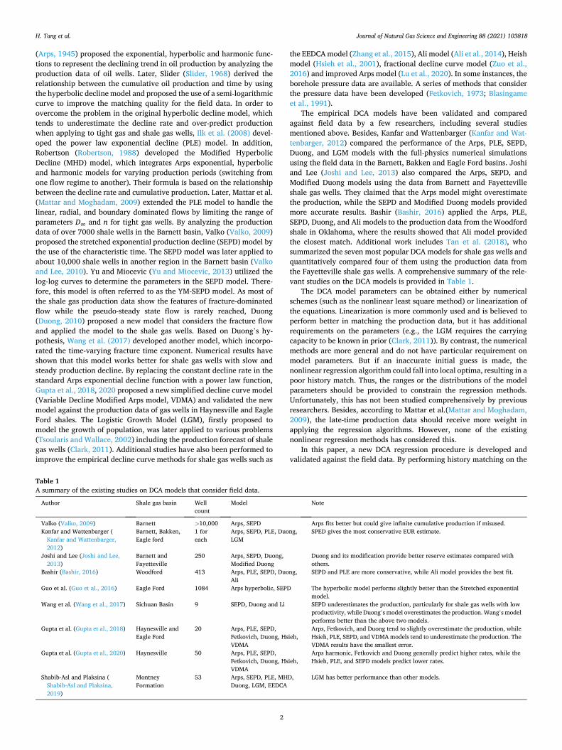
Moreover, we calculated the normalized monthly rate for all the wells, as well as their averages (Fig. 6). The production durations of the Barnett wells are much longer than those of the Marcellus wells. It is also

(a) (b)

Fig. 1. The normalized monthly production rate qn versus t (left) and the natural logarithm of normalized monthly production rate ln (qn) versus t (right) of well M3 in Barnett shale.

H. Tang et al.

Journal of Natural Gas Science and Engineering 88 (2021) 103818

6

Fig. 2. Comparisons of the historical data, history matched results with linearization method, direct nonlinear regression and the new method with various DCA models (a) SPED, (b) Duong, (c) Wang and (d) LGM using Barnett M3 well data.

Fig. 3. Comparisons of production data, fitted curve using linearization method, direct nonlinear regression and the new method with the Duong model for two wells ((a) and (b)) from Barnett and two wells ((c) and (d)) from Marcellus.

H. Tang et al.

Journal of Natural Gas Science and Engineering 88 (2021) 103818

7

seen that the production rate declines more rapidly in the Barnett wells likely due to their less advanced technologies and poorer reservoir quality as we previously mentioned.

4.2. History matching using the DCA models

We first perform well-by-well history match (curve fitting) for all the 550 gas wells selected using the Arps, PLE, SEPD, Duong, Wang, VDMA and LGM models. As described earlier, the new DCA procedure method performs better than the direct nonlinear regression method. Therefore, it is used to tune the parameters in each model. The coefficient of determination (R2) is used as a measure of the matching quality. The averages of R2 for the 550 wells are shown in Fig. 7.

In general, all the seven models can match the production history reasonably well with averaged R2 larger than 0.8. Among these models, the Wang model seems to provide the least accurate history match for

wells in both basins. The performance of other six models are compa-rable. The relatively larger error in the Wang model could be because it only has two unknown parameters while others have three plus, as more parameters give more flexibility to match the data. If the exponent of ln (t) in Wang model can be tuned, its performance becomes similar to other models. Besides, the matching quality of these models is better for Marcellus wells, which could be explained by its short production history.

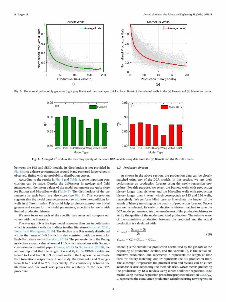
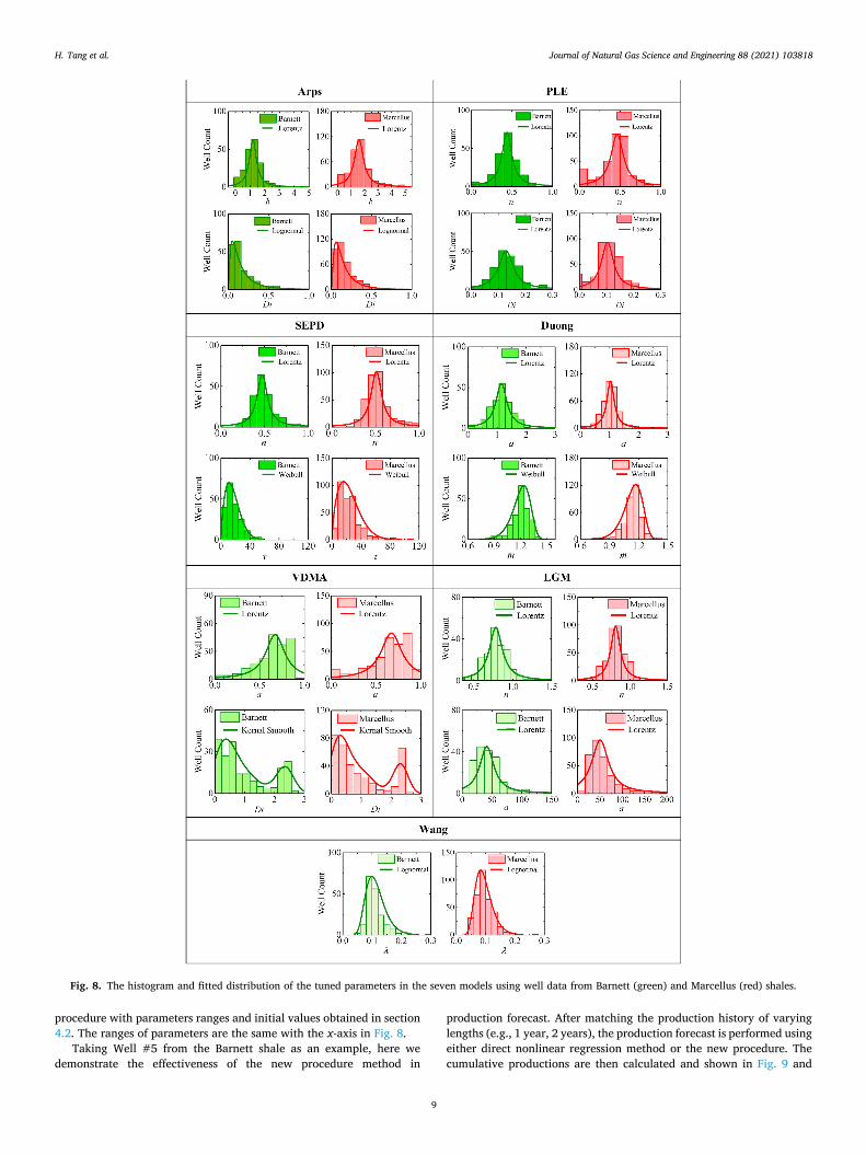
The histogram of the tuned parameters of the seven DCA models are presented in Fig. 8. The solid curves are the trend lines which fit to the histogram the best for each parameter. Some outliers are not shown. The mean values of the key model parameters in each basin are shown in Table 3. During the regression calculation, we did not pre-define the ranges of any parameter. The initial guesses are based on the average values in the literatures (Table 1). The D∞ in PLE model is smaller than 0.01 and approaches to 0 in most cases, resulting in similar performance

Fig. 4. Distribution of selected wells in the Barnett and Marcellus play. (The terrain map is from OpenCycleMap. The ranges of each play are obtained from U.S. Energy Information Administration, website: https://www.eia.gov/maps/maps.htm).

0

0.05

0.1

0.15

0.2

0.25

0.3

0 17 35 52 69 87 104

121

139

156

174

191

208

226

243

260

278

295

312

330

347

364

382

399

416

434

451

469

486

sllew fo noitroP

Peak monthly production rate [MMSCF/M]

Barnett wells Marcellus wells

Fig. 5. Histogram of the peak (or plateau) gas rate of the wells in Barnett and Marcellus.

H. Tang et al.

Journal of Natural Gas Science and Engineering 88 (2021) 103818

8

between the PLE and SEPD models. Its distribution is not provided in Fig. 8 since a dense concentration around 0 and scattered large values is observed, fitting with no probability distribution curves.

According to the results in Fig. 8 and Table 3, some important con-clusions can be made. Despite the differences in geology and field management, the mean values of the model parameters are quite close for Barnett and Marcellus wells (Table 3). The distributions of the pa-rameters in each basin are also close (see Fig. 8). This observation suggests that the model parameters are not sensitive to the conditions for wells in different basins. This could help us choose appropriate initial guesses and ranges for the model parameters, especially for wells with limited production history.

We now focus on each of the specific parameter and compare our values with the literature.

The average of b in the Arps model is greater than one in both basins which is consistent with the findings in other literature (Fan et al., 2011; Yousuf and Blasingame, 2016). The decline rate Di is mainly distributed within the range of 0–0.5 which is also consistent with the results for Eagle Ford shale wells (Guo et al., 2016). The parameter m in the Duong model has a mean value of around 1.15, which also aligns with Duong’s conclusion in his initial paper (Duong, 2012). In Gupta et al. (2018), the authors reported that the ranges of a and Di in the VDMA models are from 0 to 1 and from 0 to 3 for shale wells in the Haynesville and Eagle Ford formations, respectively. In our study, the values of a and Di ranges from 0 to 1 and 0 to 2.8, respectively. The consistency between the literature and our work also proves the reliability of the new DCA procedure.

4.3. Production forecast

As shown in the above section, the production data can be closely matched using any of the DCA models. In this section, we test their performance on production forecast using the newly regression pro-cedure. For this purpose, we select the Barnett wells with production history longer than six years and the Marcellus wells with production history longer than 4 years, which corresponds to 183 and 196 wells, respectively. We perform blind tests to investigate the impact of the length of history matching on the quality of production forecast. Once a gas well is selected, its early production is history matched to tune the DCA model parameters. We then use the rest of the production history to verify the quality of the model-predicted production. The relative error of the cumulative production between the predicted and the actual production is calculated with:

errmethod =Qmethod − Q0

Q0

Qmethod = Qti0 + QtN

method − Qtimethod

(18)

where Q is the cumulative production normalized by the gas rate at the beginning of production decline, and the variable Q0 is the actual cu-mulative production. The superscript ti represents the length of time used for history matching, and tN represents the full production time. The subscript 0 represents the practical data and method can be either nonlinear or new depending the methods used. Direct means predicting the production by DCA models using direct nonlinear regression. New means using the new regression procedure proposed in section 2.2. Qnew,

res represents the cumulative production calculated using new regression

Fig. 6. The normalized monthly gas rates (light grey lines) and their averages (thick colored lines) of the selected wells in the (a) Barnett and (b) Marcellus basins.

Arps PLE SEPD Duong Wang VDMA LGM0.80

0.85

0.90

0.95

R2

Model Type

Barnett(a)

Arps PLE SEPD Duong Wang VDMA LGM0.80

0.85

0.90

0.95

R2

Model Type

Marcellus(b)

Fig. 7. Averaged R2 to show the matching quality of the seven DCA models using data from the (a) Barnett and (b) Marcellus wells.

H. Tang et al.

Journal of Natural Gas Science and Engineering 88 (2021) 103818

9

procedure with parameters ranges and initial values obtained in section 4.2. The ranges of parameters are the same with the x-axis in Fig. 8.

Taking Well #5 from the Barnett shale as an example, here we demonstrate the effectiveness of the new procedure method in

production forecast. After matching the production history of varying lengths (e.g., 1 year, 2 years), the production forecast is performed using either direct nonlinear regression method or the new procedure. The cumulative productions are then calculated and shown in Fig. 9 and

Fig. 8. The histogram and fitted distribution of the tuned parameters in the seven models using well data from Barnett (green) and Marcellus (red) shales.

H. Tang et al.

Journal of Natural Gas Science and Engineering 88 (2021) 103818

10

Fig. 10. The Arps, PLE, Duong, Wang, VDMA and LGM models are considered.

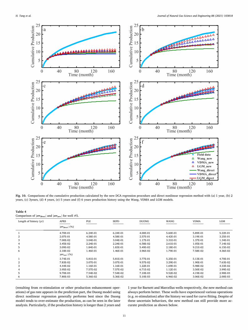
In Figs. 9 and 10, the cyan points represent the field data, the tri-angles represent the results calculated by our new procedure while the solid lines are the results from direct nonlinear regression. First of all, it is apparent that longer production history matching results in more accurate prediction in cumulative production, although the

improvement on the accuracy gets smaller when history matching period is longer than three years. Another important observation is that for almost all the six DCA models, results using the new regression procedure are consistently more accurate than using the direct nonlinear regression method, no matter how long the history is used to match the model. The effectiveness of the newly proposed DCA procedure is clearly demonstrated in Figs. 9 and 10.

In addition to Figs. 9 and 10, we show the magnitude of the relative error on cumulative production for results using the direct nonlinear regression method and our new method in Table 4. The errors are plotted in Fig. 11 as bar charts. As expected, more accurate results are obtained by the use of the new regression procedure.

We then repeat the above procedures all of the wells from the Barnett and Marcellus basins, and compare their errors in a statistical manner. Fig. 12 shows the magnitude of the averaged relative errors for the DCA models using the direct nonlinear regression method and new regression procedure with varying lengths of production history. Though the direct nonlinear regression performs better in a few cases, in most situations, the new method can predict the cumulative production more accurate than direct nonlinear regression. A major reason that our method fails to perform better than direct nonlinear regression in certain cases is that a significant change of production data might occur in the prediction period. For example, for the cases when an unexpected increase

Table 3 Averages of model parameters for wells in Barnett (B) and Marcellus (M) shales.

Parameters Average-B Average-M Parameters Average-B Average-M

Arps PLE b 1.18 1.68 n 0.43 0.43 Di 0.22 0.18 Di 0.13 0.10

D∞ 0.0036 0.0040 SEPD Duong n 0.50 0.54 a 1.12 1.00 τ 16.82 24.12 m 1.20 1.14 Wang VDMA λ 0.11 0.10 a 0.63 0.63

Di 0.99 0.95 EEDCA LGM βe 0.54 0.53 n 0.77 0.80 n 0.23 0.24 a 159.03 237.67

0 40 80 120 160

5

10

15

20

25

0 40 80 120 160

5

10

15

20

25

0 40 80 120 160

5

10

15

20

25

0 40 80 120 160

5

10

15

20

25

0 40 80 120 160

5

10

15

20

25

0 40 80 120 160

5

10

15

20

25

noitcudorP evitalumu

C

Time (month)

aC

umul

ativ

e Pr

oduc

tion

Time (month)

b

noitcudorP evitalumu

C

Time (month)

c

Cum

ulat

ive

Prod

uctio

n

Time (month)

d

noitcudorP evitalumu

C

Time (month)

e

Cum

ulat

ive

Prod

uctio

n

Time (month)

Field data Arps_new PLE_new Duong_new Arps-direct PLE_direct Duong_direct

f

Fig. 9. Comparisons of the cumulative production calculated by the new DCA regression procedure and direct nonlinear regression method with (a) 1 year, (b) 2 years, (c) 3years, (d) 4 years, (e) 5 years and (f) 6 years production history using the Arps, PLE and Duong models.

H. Tang et al.

Journal of Natural Gas Science and Engineering 88 (2021) 103818

11

(resulting from re-stimulation or other production enhancement oper-ations) of gas rate appears in the prediction part, the Duong model using direct nonlinear regression generally performs best since the Duong model tends to over-estimate the production, as can be seen in the later analysis. Particularly, if the production history is longer than 2 years and

1 year for Barnett and Marcellus wells respectively, the new method can always perform better. These wells have experienced various operations (e.g. re-stimulation) after the history we used for curve fitting. Despite of these uncertain behaviors, the new method can still provide more ac-curate prediction as shown below.

0 40 80 120 160

5

10

15

20

25

0 40 80 120 160

5

10

15

20

25

0 40 80 120 160

5

10

15

20

25

0 40 80 120 160

5

10

15

20

25

0 40 80 120 160

5

10

15

20

25

0 40 80 120 160

5

10

15

20

25

noitcudorP evitalumu

C

Time (month)

a

Cum

ulat

ive

Prod

uctio

n

Time (month)

bnoitcudorP evitalu

muC

Time (month)

c

Cum

ulat

ive

Prod

uctio

nTime (month)

d

noitcudorP evitalumu

C

Time (month)

e

Cum

ulat

ive

Prod

uctio

n

Time (month)

Field data Wang_new VDMA_new LGM_new Wang_direct VDMA_direct LGM_direct

f

Fig. 10. Comparisons of the cumulative production calculated by the new DCA regression procedure and direct nonlinear regression method with (a) 1 year, (b) 2 years, (c) 3years, (d) 4 years, (e) 5 years and (f) 6 years production history using the Wang, VDMA and LGM models.

Table 4 Comparison of |errdirect| and |errnew| for well #5.

Length of history (yr) APRS PLE SEPD DUONG WANG VDMA LGM

|errdirect| (%)

1 4.70E-01 6.24E-01 6.24E-01 4.00E-01 5.60E-01 5.89E-01 5.22E-01 2 2.07E-01 4.58E-01 4.58E-01 2.57E-01 4.42E-01 3.19E-01 3.25E-01 3 7.00E-02 3.04E-01 3.04E-01 1.17E-01 3.31E-01 1.37E-01 1.34E-01 4 3.45E-02 2.24E-01 2.24E-01 6.58E-02 2.61E-01 1.05E-01 7.14E-02 5 3.09E-02 1.84E-01 1.83E-01 5.49E-02 2.18E-01 9.21E-02 6.15E-02 6 2.18E-02 1.46E-01 1.46E-01 3.96E-02 1.79E-01 7.58E-02 4.36E-02

|errnew| (%) 1 3.74E-01 5.81E-01 5.81E-01 3.77E-01 5.25E-01 5.13E-01 4.70E-01 2 7.83E-02 3.07E-01 3.07E-01 9.57E-02 3.29E-01 1.90E-01 7.63E-02 3 4.44E-02 1.16E-01 1.16E-01 1.22E-01 1.69E-01 5.98E-02 4.33E-02 4 3.95E-02 7.57E-02 7.57E-02 6.71E-02 1.12E-01 3.50E-02 3.99E-02 5 9.70E-03 7.54E-02 7.54E-02 7.10E-03 9.52E-02 4.19E-02 2.90E-03 6 7.80E-03 5.36E-02 5.36E-02 5.10E-03 6.96E-02 3.06E-02 2.00E-03

H. Tang et al.

Journal of Natural Gas Science and Engineering 88 (2021) 103818

12

To investigate the impact of initial guess on DCA model performance, we use the initial guess for each parameter with the values shown in Table 3 and repeat the history matching and production forecast pro-cedures for all wells. The results are shown in Fig. 13. From this figure, we see negative values for most of the models, which indicates that a careful choose of initial guess for each parameter could lead to more accurate results.

The above results clearly demonstrated the superior performance of the new regression procedure in both history matching and production forecast compared to the commonly-used direct nonlinear regression method. To further investigate the performance of the DCA models with the new regression procedure, we also plot the relative errors of each model for cases with varying lengths of production history in Fig. 14. Consistent with the results for Well #5, the error gets smaller as longer history is used. If we only use the first year’ production data for history

matching, the predicted cumulative gas production could have signifi-cant error. Consistent with the conclusions made by Johanson (Johan-son, 2013), the mean values of predictions become over 10% closer to the actual production values by increasing the history to 2 years. Ac-cording to the definition of relative error in Eq. (18), a positive value of errnew indicates an over-estimate of the cumulative production, and a negative value of errnew indicates an under-estimate of the cumulative production. It is shown that for both basins, the Arps and Duong models tend to overestimate the production while the PLE and SEPD models tend to under-estimate the production, which agrees with previous studies (Table 1). The Wang, VDMA and LGM predict the least error, though they tend to underestimate the production when history matching is less than two years.

0.00E+00

2.00E-01

4.00E-01

6.00E-01

8.00E-01

1 2 3 4 5 6Length of produc�on history (years)

0.00E+00

2.00E-01

4.00E-01

6.00E-01

8.00E-01

1 2 3 4 5 6Length of produc�on history (years)

APRSPLESEPDDUONGWANGVDMALGM

(a) (b)

Fig. 11. Comparisons of the magnitude of the relative error in cumulative production for DCA models using the direct nonlinear regression and the new regression procedure for Well #5.

(a) (b)

-4

-2

0

2

Arps PLE SEPD Duong Wang VDMA LGM

Model Type

Marcellus wells

1 yr 2 yrs 3 yrs 4 yrs

(%)

-4

-2

0

2

4

Arps PLE SEPD Duong Wang VDMA LGM

Model Type

Barne� wells

1 yr 2 yrs 3 yrs 4 yrs 5 yrs 6 yrs

(%)

Fig. 12. Difference of averaged absolute values of cumulative production difference between the direct and the new nonlinear regression procedure for (a) Barnett and (b) Marcellus wells.

-1.5

-1

-0.5

0

0.5

Arps PLE SEPD Duong Wang VDMA LGM

Model Type

Barne� wells

1 yr 2 yrs 3 yrs 4 yrs 5 yrs 6 yrs

(%)

-1.5

-1

-0.5

0

0.5

Arps PLE SEPD Duong Wang VDMA LGM

Model Type

1 yr 2 yrs 3 yrs 4 yrs

(%)

(a) (b)

Fig. 13. Difference in relative errors for cases using restricted and unbounded parameters for (a) Barnett wells and (b) Marcellus wells.

H. Tang et al.

Journal of Natural Gas Science and Engineering 88 (2021) 103818

13

5. Conclusions

In this paper, a systematic study was performed to investigate the performance of the Arps, PLE, SEPD, Duong, Wang, VDMA and LGM models using field data from over 500 Barnett and Marcellus shale gas wells. We proposed a new data transformation method, which converts both the production data and model prediction into logarithmic space. By combing it with the nonlinear regression algorithm, the new DCA procedure is capable of capturing the trend of late time production decline. According to the numerical results presented in this paper, the following conclusions are drawn:

(1) Compared to the linearization and direct nonlinear regression method, the new DCA regression procedure is able to match the late-time production data much more closely. Therefore, a more accurate production forecast can be achieved by the use of the new regression method. This is verified using the field data from the Barnett and Marcellus shale wells.

(2) All the above-mentioned DCA models are able to match the production history closely. After history matching, the final tuned parameters for each model in the two basins are similar. The statistical distribution of each parameter can provide reliable initial guess and range for other wells, especially for wells with limited production history.

(3) As expected, longer history leads to more accurate production forecast. If only one year’s production history is included, a sig-nificant error will occur no matter which DCA model or regres-sion method is used.

(4) Based on our observation, the Arps and Duong models tend to overestimate the production, while the PLE and SEPD models are more likely to underestimate the production. The Wang, VDMA and LGM models have the best performance in terms of produc-tion forecast, especially when production data over two years is used for history matching.

Credit author statement

Huiying Tang: Conceptualization, Methodology, Writing- Original draft preparation. Boning Zhang: Investigation, Validation. Sha Liu: Data processing. Hangyu Li: Supervision, Writing-Reviewing and Edit-ing. Da Huo: Reviewing and Editing. Yu-Shu Wu: Reviewing and Editing.

Declaration of competing interest

The authors declare that they have no known competing financial interests or personal relationships that could have appeared to influence the work reported in this paper.

Acknowledgement

This work was supported by the National Natural Science Foundation of China (Grant No. 51904257, 51874251), the open foundation of State Key Laboratory of Oil and Gas Reservoir Geology and Exploitation (Southwest Petroleum University) (Grant No. PLM201819) and the Science Foundation of Sichuan Province (Grant No. 2019JDRC0089).

References

Akbarnejad-Nesheli, B., 2012. Stretched Exponential Decline Model as a Probabilistic and Deterministic Tool for Production Forecasting and Reserve Estimation in Oil and Gas Shales. PhD dissertation. Texas A&M University.

Ali, T., Sheng, J., Soliman, M., 2014. New production-decline models for fractured tight and shale reservoirs. In: SPE Western North American and Rocky Mountain Joint Meeting, 16-18 April. Society of Petroleum Engineers, Denver, Colorado, USA.

Arps, J.J., 1945. Analysis of decline curves. Transactions of the AIME 160 (1), 228–247. Baihly, J.D., Malpani, R., Altman, R., Lindsay, G., Clayton, R., 2015. Shale gas production

decline trend comparison over time and basins—revisited. In: Unconventional Resources Technology Conference, 20-22 July. Society of Exploration Geophysicists, American Association of Petroleum Geologists, Society of Petroleum Engineers, San Antonio, Texas, USA.

Bashir, M.O., 2016. Decline curve analysis on the Woodford shale and other major shale plays. In: SPE Western Regional Meeting, 23-26 May. Society of Petroleum Engineers, Anchorage, Alaska, USA.

Bello, R.O., Wattenbarger, R.A., 2010. Multi-stage hydraulically fractured horizontal shale gas well rate transient analysis. In: North Africa Technical Conference and Exhibition, 14-17 February. Society of Petroleum Engineers, Cairo, Egypt.

Blasingame, T.A., McCray, T.L., Lee, W.J., 1991. Decline curve analysis for variable pressure drop/variable flowrate systems. In: SPE Gas Technology Symposium, 23-24 January. Society of Petroleum Engineers, Houston, Texas, USA.

Clark, A.J., 2011. Decline Curve Analysis in Unconventional Resource Plays Using Logistic Growth Models. Master Dissertation. University of Texas at Austin.

Duong, A.N., 2010. An unconventional rate decline approach for tight and fracture- dominated gas wells. In: Canadian Unconventional Resources and International Petroleum Conference, 19-21 October. Society of Petroleum Engineers, Calgary, Alberta, Canada.

Duong, A.N., 2012. Rate-decline analysis for fracture-dominated shale reservoirs. SPE Reservoir Eval. Eng. 14 (3), 377–387.

Fan, L., Luo, F., Lindsay, G., Thompson, J., Robinson, J., 2011. The bottom-line of horizontal well production decline in the Barnett shale. In: SPE Production and Operations Symposium, 27-29 March. Society of Petroleum Engineers, Oklahoma City, Oklahoma, USA.

Fetkovich, M.J., 1973. Decline curve analysis using type curves. In: Fall Meeting of the Society of Petroleum Engineers of AIME, 30 September - 3 October. Society of Petroleum Engineers, Las Vegas, Nevada, USA.

Fulford, D.S., Blasingame, T.A., 2013. Evaluation of time-rate performance of shale wells using the transient hyperbolic relation. In: SPE Unconventional Resources Conference - Canada, 5-7 November. Society of Exploration Geophysicists, American Association of Petroleum Geologists, Society of Petroleum Engineers, Calgary, Alberta, Canada.

Guo, K., Zhang, B., Aleklett, K., Hook, M., 2016. Production patterns of Eagle Ford shale gas: decline curve analysis using 1084 wells. Sustainability 8 (10), 973.

Gupta, I., Rai, C., Sondergeld, C., Devegowda, D., 2018. Variable exponential decline- modified Arps to characterize unconventional shale production performance. In: SPE/AAPG/SEG Unconventional Resources Technology Conference, 23-25 July. Society of Exploration Geophysicists. American Association of Petroleum Geologists, Society of Petroleum Engineers, Houston, Texas, USA.

-15

-10

-5

0

5

10

15

Arps PLE SEPD Duong Wang VDMA LGM

Model Type

Marcellus wells

1 yr 2 yrs 3 yrs 4 yrs

(%)

(a) (b)

-35

-20

-5

10

25

Arps PLE SEPD Duong Wang VDMA LGM

Model Type

Barne� wells

1 yr 2 yrs 3 yrs 4 yrs 5 yrs 6 yrs

(%)

Fig. 14. Relative difference between predicted and practical cumulative production for (a) Barnett wells and (b) Marcellus wells.

H. Tang et al.

Journal of Natural Gas Science and Engineering 88 (2021) 103818

14

Gupta, I., Rai, C., Devegowda, D., Sondergeld, C., 2020. Haynesville Shale: predicting long-term production and residual analysis to identify well Interference and fracture hits. SPE Reservoir Eval. Eng. 23 (1), 132–142.

Hakso, A., Zoback, M., 2019. The relation between stimulated shear fractures and production in the Barnett Shale: implications for unconventional oil and gas reservoirs. Geophysics 84 (6), B461–B469.

Hsieh, F.S., Vega, C., Vega, L., 2001. Applying a time-dependent Darcy equation for decline analysis for wells of varying reservoir type. In: SPE Rocky Mountain Petroleum Technology Conference, 21-23 May. Society of Petroleum Engineers, Keystone, Colorado, USA.

Ilk, D., Rushing, J.A., Perego, A.D., Blasingame, T.A., 2008. Exponential vs. hyperbolic decline in tight gas sands: understanding the origin and implications for reserve estimates using Arps’decline curves. In: SPE Annual Technical Conference and Exhibition, 21–24 September. Society of Petroleum Engineers, Denver, Colorado, USA.

Johanson, B.L., 2013. Deterministic and Stochastic Analyses to Quantify the Reliability of Uncertainty Estimates in Production Decline Modeling of Shale Gas Reservoirs. PhD dissertation. Colorado School of Mines.

Joshi, K., Lee, W.J., 2013. Comparison of various deterministic forecasting techniques in shale gas reservoirs. In: SPE Hydraulic Fracturing Technology Conference, 4-6 February. Society of Petroleum Engineers, The Woodlands, Texas, USA.

Kanfar, M., Wattenbarger, R., 2012. Comparison of empirical decline curve methods for shale wells. In: SPE Canadian Unconventional Resources Conference, 30 October - 1 November. Society of Petroleum Engineers, Calgary, Alberta, Canada.

Lee, W.J., Sidle, R., 2010. Gas-reserves estimation in resource plays. SPE Econ. Manag. 2 (2), 86–91.

Lu, H., Ma, X., Azimi, M., 2020. US natural gas consumption prediction using an improved kernel-based nonlinear extension of the Arps decline model. Energy 194, 116905.

Mattar, L., Moghadam, S., 2009. Modified power law exponential decline for tight gas. In: Canadian International Petroleum Conference (CIPC), 16-18 June. Petroleum Society of Canada, Calgary, Alberta, Canada.

Meng, Q., Hou, G., 2012. Characteristics and implications of Marcellus shale gas reservoir: appalachian Basin. China Petrol. Explor. 17 (1), 65–73.

Pierre-François, V., 1838. Notice sur la loi que la population poursuit dans son accroissement. Corresp. Math. Phys 10, 113–121.

Powell, M.J.D., Yuan, Y., 1991. A trust region algorithm for equality constrained optimization. Math. Program. 49 (1–3), 189–211.

Robertson, S., 1988. Generalized Hyperbolic Equation. Society of Petroleum Engineers, Richardson, TX, USA.

Samandarli, O., Al Ahmadi, H.A., Wattenbarger, R.A., 2011. A Semi-analytic method for history matching fractured shale gas reservoirs. In: SPE Western North American Region Meeting, 7-11 May. Society of Petroleum Engineers, Anchorage, Alaska, USA.

Shabib-Asl, A., Plaksina, T., 2019. Selection of decline curve analysis model using Akaike information criterion for unconventional reservoirs. J. Petrol. Sci. Eng. 182, 106327.

Slider, H.C., 1968. A simplified method of hyperbolic decline curve analysis. J. Petrol. Technol. 20 (3), 235–236.

Stalgorova, E., Mattar, L., 2012. Analytical model for history matching and forecasting production in multifrac composite systems. In: SPE Canadian Unconventional Resources Conference, 30 October-1 November. Society of Petroleum Engineers, Calgary, Alberta, Canada.

Tan, L., Zuo, L., Wang, B., 2018. Methods of decline curve analysis for shale gas reservoirs. Energies 11 (3), 552.

Tsoularis, A., Wallace, J., 2002. Analysis of logistic growth models. Math. Biosci. 179 (1), 21–55.

Valko, P.P., 2009. Assigning value to stimulation in the Barnett Shale: a simultaneous analysis of 7000 plus production histories and well completion records. In: SPE Hydraulic Fracturing Technology Conference, 19-21 January. Society of Petroleum Engineers, The Woodlands, Texas, USA.

Valko, P.P., Lee, W.J., 2010. A better way to forecast production from unconventional gas wells. In: SPE Annual Technical Conference and Exhibition, 19-22 September. Society of Petroleum Engineers, Florence, Italy.

Wang, K., Li, H., Wang, J., Jiang, B., Bu, C., Zhang, Q., 2017. Predicting production and estimated ultimate recoveries for shale gas wells: a new methodology approach. Appl. Energy 206, 1416–1431.

Wang, Q., Song, X., Li, R., 2018. A novel hybridization of nonlinear grey model and linear ARIMA residual correction for forecasting US shale oil production. Energy 165, 1320–1331.

Wang, H., Chen, L., Qu, Z., Yin, Y., Kang, Q., Yu, B., Tao, W., 2020. Modeling of multi- scale transport phenomena in shale gas production-A critical review. Appl. Energy 262, 114575.

Yao, J., Sun, H., Fan, D., Huang, Z., Sun, Z., Zhang, G., 2013. Numerical simulation of gas transport mechanisms in tight shale gas reservoirs. Petrol. Sci. 10 (4), 528–537.

Yousuf, W., Blasingame, T.A., 2016. New Models for time-cumulative behavior of unconventional reservoirs—diagnostic relations, production forecasting, and EUR methods. In: Unconventional Resources Technology Conference, 1-3 August. Society of Exploration Geophysicists, American Association of Petroleum Geologists, Society of Petroleum Engineers, San Antonio, Texas, USA.

Yu, S., Miocevic, D.J., 2013. An improved method to obtain reliable production and EUR prediction for wells with short production history in tight/shale reservoirs. In: Unconventional Resources Technology Conference, 12-14 August. American Association of Petroleum Geologists, Society of Petroleum Engineers, Denver, Colorado, USA.

Zeng, B., Duan, H., Bai, Y., Meng, W., 2018. Forecasting the output of shale gas in China using an unbiased grey model and weakening buffer operator. Energy 151, 238–249.

Zhang, H., Cocco, M., Rietz, D., Cagle, A., Lee, J., 2015. An empirical extended exponential decline curve for shale reservoirs. In: SPE Annual Technical Conference and Exhibition, 28-30 September. Society of Petroleum Engineers, Houston, Texas, USA.

Zuo, L., Yu, W., Wu, K., 2016. A fractional decline curve analysis model for shale gas reservoirs. Int. J. Coal Geol. 163, 140–148.

H. Tang et al.