Discussion Papers in Economics

How Does Poverty Decline? Evidence from India, 1983-1999

Mukesh Eswaran Ashok Kotwal

Bharat Ramaswami and

Wilima Wadhwa

March 2007

Discussion Paper 07-05

Indian Statistical Institute, Delhi Planning Unit

7 S.J.S. Sansanwal Marg, New Delhi 110 016, India

How Does Poverty Decline?Evidence from India, 1983-1999

ByMukesh Eswaran, Ashok Kotwal, Bharat Ramaswami, and Wilima Wadhwa*

March 2007

ABSTRACT

This paper attempts to assess the relative contributions of the farm and non-farm sectors

to the increase in agricultural wage earnings in India between 1983-1999. Cross-section

analysis of NSS data for 1983 and 1993 confirm the importance of farm productivity

growth, consistent with the predictions of our theoretical model. A counterfactual

exercise that attempts to estimate the relative contribution of the non-farm sector to the

increase in the agricultural wage earnings during the period 1983-1999 suggests that this

figure is no more than 25% at the all-India level, though it is higher in some states. Thus

the bulk of the growth in wage earnings and the attendant decline in poverty during this

period appears to be due to the farm sector.

Keywords: Farm and non-farm productivity growth, non-farm employment, poverty, wage earningsJEL Classification Numbers: O13, O14, O53

* At University of British Columbia (eswaran@econ.ubc.ca), University of British Columbia(kotwal@econ.ubc.ca), Indian Statistical Institute (bharat@isid.ac.in), and (wwadhwa@uci.edu),respectively.Acknowledgements : We would like to thank Paul Beaudry, Andrew Foster, Peter Lanjouw, DilipMookherjee, Suresh Tendulkar, Alessandro Tarrozi, the participants of the World Bank workshop onEquity and Development (December 7-8, 2004) and the participants of the ‘Workshop on the IndianEconomy: Policy and Performance 1980-2000’ held at the Centre for India and South Asia Research,UBC in Vancouver (in June 2005) for their helpful comments. We are grateful to the Shastri Indo-Canadian Institute for financial support through the SHARP programme.

1

1. Introduction

In a less developed country, the most consequential aspect of GDP growth is the

impact it has on poverty. A convincing empirical case has been made in the literature

that higher growth translates into lower poverty [e.g., Besley and Burgess (2003), Dollar

and Kraay (2002), Kraay (2004), Ravallion (2001)]. Using cross-country data for a

number of years, Besley and Burgess estimate that a 1% increase in GDP growth reduces,

on average, poverty by 0.73%. However, the average impact hides variation between

countries. For example, the elasticity of poverty with respect to economic growth is –1 in

East Asia but only –0.59 in South Asia (Besley and Burgess). In order to be able to

discriminate among policies promoting growth, we need to understand the process by

which different growth strategies impinge on the incomes of the poor. The purpose of

this paper is to propose a framework that would enable us to analyze such a process by

drawing lessons from the last two decades of growth and poverty decline in India. More

specifically, we will try to evaluate whether it is the productivity growth in agriculture or

in non-agriculture that has a bigger impact on poverty decline.

Such a sectoral decomposition of growth and its impact on poverty is valuable

because the sector amenable to faster growth may not be the one whose growth has a

greater impact on poverty. Typically, the non-farm sector in developing countries

exhibits higher rates of growth since non-farm technology can be transferred more easily

from developed countries; it may need less climatic adaptation. It is also the case that,

unlike the farm sector, it is not crucially dependent on a fixed factor like land. Yet, a

significant part of the labor force in developing countries makes its living in agriculture.

A well-known statistic is that the poorer the country, the greater is the share of the labor

2

force in agriculture. How does the growth in the non-farm part of GDP translate into a

boost in the incomes of those working in the farm sector? This question must be

answered in order to understand the process by which poverty declines. If during a

period of high growth, poverty also declines, it does not follow that the faster-growing

sector is mostly responsible for it. It is quite possible that growth is mostly attributable to

one sector and the poverty decline to the other.

India is one of the fastest growing economies in the world today. It also has the

dubious distinction of having the largest share of the world’s poor. In addition, it has

some of the better quality data among the developing countries. It therefore makes an

ideal case study for our purpose. Since the early 1980’s, India has enjoyed an average

GDP growth rate of 5.5 per cent per annum. More importantly, the proportion of the

population below the poverty line declined from about 44.5% in 1983-84 to 26% in 1999-

00. It is instructive, therefore, to examine the process through which the policies

responsible for growth may have raised the incomes of the poor. It is worth noting that

agricultural GDP grew at a much lower rate than the non-farm GDP from 1980-2000.

Agricultural GDP grew at a rate of 3.36% in the 80’s and at 2.5% in the 90’s. Industry

and services grew at 7.54% and 6.23% in the 80’s and at 5.6% and 7.07% in the 90’s

respectively. An important question is: which sector contributed more toward the

observed poverty decline?

2. Literature

Using country level panel data sets, several researchers (cited in the introduction)

have looked at the growth-poverty relationship. This literature finds a strong negative

3

association between growth and poverty. However, this is the relationship on average,

and country (and regional) experiences could be diverse. As Ravallion (2001) points out,

the growth-poverty link may be quite weak in the face of rising inequality.

An identity links changes in the level of poverty in any given country with

changes in the average income level (i.e., growth) and changes in income inequality.

Changes in poverty can therefore be decomposed into a growth and a distribution

component and their relative importance can be quantified. Besley, Burgess and Esteve-

Volart (2004) undertake such an exercise for different states of India revealing the

heterogeneity of the growth-poverty link. This finding calls for a deeper examination

beyond growth-poverty correlations.

Cross-country regressions that relate inequality or poverty to the variables that

have been known to be robust correlates of growth (“rule of law”, openness to

international trade, inflation, size of government, measure of financial development) have

pretty much drawn a blank [Dollar and Kraay (2002), Kraay (2004), Lopez (2004)].

Kray (2004) and Ravallion (2001) conclude that country-specific research is necessary to

understand heterogenous outcomes (of growth) for the poor.

In the Indian case, scholars have used state level panel data to establish the

correlates of poverty. Ravallion and Datt (1996) find rural economic growth to have a

significant impact in reducing urban and rural poverty while urban growth has little

impact on rural poverty. In the rural sector, higher farm yield is the key variable that

reduces poverty [Datt and Ravallion (1998)]. On the other hand, the impact of non-farm

economic growth varies across states, depending on initial conditions [Datt and

Ravallion (2002)]. In a similar analysis of panel data, Besley, Burgess and Esteve-Volart

4

(2004) report opposite results. They find economic growth in the secondary and tertiary

sectors to contribute more to poverty reduction than primary sector growth. State level

panel data has also been used to examine the impact of specific policies on poverty –

including labour regulation [Besley and Burgess (2004)], land reform legislation [Besley

and Burgess (2002)] and expansion of rural banking [Burgess and Pande (2005)].

Topalova (2005) assembled a district level panel data set and used it to establish that

districts that experienced greater tariff reductions recorded slower decrease in poverty.

Finally, Palmer-Jones and Sen (2003) is an instance of a cross-sectional analysis at the

region level (intermediate between districts and states) where they relate rural poverty to

agricultural growth and several control variables. Useful as they are in enhancing our

empirical knowledge of which policies were associated with greater poverty reduction,

these analyses have not established the causal mechanisms by which the poor have

gained from the growth process.

In a recent study, Foster and Rosenzweig (2003, 2004) present a causal

framework that links agricultural productivity increase and capital flows into the rural

factory sector on the one hand with the agricultural wages on the other. They test this

framework with panel data (not yet in the public domain) over the years 1983 through

1999. They find that in their framework agricultural productivity improvement

increases inequality across regions while the rural factory sector helps to decrease it.

They argue that it is only the non-traded segment of the rural non-farm sector that is

positively affected by agricultural growth. The traded non-farm sector (consisting of

rural factories) competes with the farm sector for labour and is therefore attracted to

regions with low agricultural productivity. Their empirical results show that much of

5

the growth in the rural non-farm sector in India was due to the rural factory sector and

not due to the non-traded sector. Furthermore, the growth in the rural factory sector

was important in accounting for the increase in rural wages over the period 1982-99.

We have two points of departure from Foster and Rosenzweig (2003, 2004). First,

at the theoretical level, we model preferences more realistically by incorporating

Engel’s law. This matters because the nature of consumer demand determines how

labour is released from agriculture (which exhibits diminishing returns) following a

productivity increase. Second, at the empirical level, we use national sample survey

data that is publicly available. Our model, however, is simpler than that of Foster and

Rosenzweig (2003, 2004) in other respects: it has only two as opposed to three sectors.

Our focus is to assess the relative contributions of productivity growths in the farm and

non-farm sectors to the observed growth in wages rather than evaluate their impact on

the regional distribution.

3. Using Agricultural Wages as a Poverty Measure

Official estimates of head-count ratios of poverty in India are computed from

national expenditure surveys and a poverty line developed by the Planning Commission.

Due to a change in the survey design in 1999 relative to 1993, the rate and direction of

change in poverty in the 1990’s cannot be established in a straightforward way.

Adjustments have to be made to render the surveys comparable and this has generated a

large debate about the merits of different types of ‘adjusted’ poverty measures.1 The

official poverty lines have also been criticized for the way in which they are updated

1 See the collection of papers in Deaton and Kozel (2005).

6

from survey to survey. Deaton and Tarozzi (2005) and Deaton (2001) have proposed

alternative price deflators which yield poverty lines and poverty measures that are

different from the official estimates. This underscores another difficulty with

conventional poverty measures: they are sensitive to the distribution of the population

around the poverty line, and so results could vary widely depending on the choice of the

poverty line.

This paper sidesteps these measurement issues by choosing to work with

agricultural wages. It is well known that agricultural laborers constitute a large fraction

of the poor in India and that their wages have a strong negative correlation with the

headcount ratios. A recent study that documents this association is Kijima and Lanjouw

(2005) who show agricultural wage rates at the region level to be strongly (inversely)

correlated with region-level poverty rates in the three years between 1987 and 1999 for

which such survey data were available.

Deaton and Dreze (2002) argue that agricultural wages can be taken not just as a

proxy for poverty but as a poverty measure in its own right since it is the reservation

wage of the very poor. It would also seem that it would be easier to theorize and model

agricultural wages than it would be for poverty measures which are complicated non-

linear functions of underlying average income and of income inequality.

To see the logic of our argument, consider a dual economy comprising a farm and

a non-farm sector. Total factor productivity (TFP) in farm and non-farm sectors can be

thought of as exogenous to this model. The connection between farm TFP and

agricultural wage is quite direct: at the same level of production inputs an increase in

agricultural TFP will raise the marginal product of labor and hence the wage. What is

7

the relationship between non-farm TFP and agricultural wages? Here the link is

through labor allocation: if an increase in non-farm TFP increases the value of the

marginal product of labor in the non-farm sector, it will draw labor away from

agriculture and, given the diminishing returns due to land (a fixed factor), the

agricultural wage will rise. The extent of the wage increase due to non-farm TFP

growth would depend, of course, on the amount of labor drawn away from agriculture.

In China, the percentage of labor force engaged in agriculture plummeted from 70% in

1979 to 47% in 1999. In other East Asian countries, like Taiwan and South Korea, this

process of structural transformation was equally swift.

In India, the reduction of labor force in agriculture has been nothing like what was

witnessed in East Asia. Estimates from employment surveys show that the share of

agriculture in the labor force for males (measured in person days) declined from about

60% in 1983 to 53% in 1999-00. As the share of manufacturing has changed very little

over these 16 years, the share of services has increased by about the same percentage.

For females, the sectoral pattern of employment has remained stagnant. 72% of female

labor force continued to be employed in agriculture in 1999-00 compared to 74% in

1983.

For 15 major Indian states, Figure 1 plots the average real daily wages (in 1999

rupees) in agriculture against the labour-land ratio (days per hectare of gross cropped

area) for 1983 and 1999. It can be seen that for all but four states (Kerala, Haryana,

Punjab and Rajasthan), the labour use per hectare of land has increased over this period.

Yet, for all but one state (Assam), real wages have increased during this period. At the

All-India level, real daily wages increased by 69% between 1983 and 1999. Quite

8

clearly, if either farm TFP or agricultural inputs such as fertilizers had not increased

during this period, agricultural wages would have declined. It becomes interesting,

therefore, to ask how much the non-farm sector growth has contributed to the growth of

agricultural wages.

4. A Theoretical Framework

To isolate the contributions of the farm and non-farm sectors to the growth of the

Indian economy, we adopt the dual economy framework that harks back to Lewis (1954)

but later modeled, as in Matsuyama (1992) and Eswaran and Kotwal (1993), with

neoclassical labour markets. We set out a model of a typical ‘regional’ economy, where a

‘region’ could mean—depending on our focus—the entire country, a state within the

country, a district, or even a village. (Whether the region should be treated as a closed

economy or as an open economy within the country will be dealt with below.) There are

two sectors within the region: a farm sector (which produces an aggregate good, food)

and a non-farm sector (which produces an aggregate of all other goods). Food production

requires labour and land, whereas non-farm output requires only labour.

The total amount of land is fixed in the region. Since the distribution of income is

not a primary focus of attention here, we assume that land is uniformly divided across all

agents. There are L agents in the economy, each inelastically providing one unit of

labour. Since land is only used in farming, labour is the only input whose allocation

across the two sectors needs to be determined in the general equilibrium.

It is our contention that the preferences of agents over farm and non-farm

products in their consumption are an important determinant of the allocation of labour

9

across these two sectors. The assumption of homothetic preferences does not ring true in

the context of developing countries, for they imply linear Engel curves. As Engel

observed over a century ago, when income increases, the proportion of income

consumers spend on food remains high initially and then declines quite rapidly. Explicit

attempts to incorporate non-homothetic preferences were made in Matsuyama (1992),

which employs Stone-Geary preferences, and Eswaran and Kotwal (1993), which invokes

lexicographic (‘hierarchical’) preferences with satiation with respect to the farm product

but not the non-farm product.

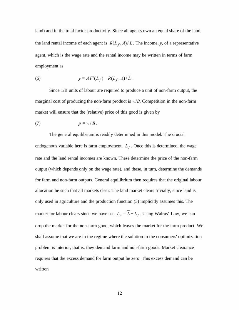
To capture the essential features of Engel's Law, albeit in stark form, we posit

here that agents have quasi-linear preferences over the two consumption goods. The

utility function, ),( zxU , representing a consumer’s preferences is given by:

(1) 0,)(),( >+= γγ zxuzxU ,

where x and z denote her consumption of farm and non-farm goods, respectively. We

assume that the sub-utility function satisfies 0(.),0(.) <′′>′ uu , and (.)u′ goes to infinity

as its argument goes to zero, that is, the farm good is essential. The marginal utility of

this good declines with consumption, while that of the non-farm good is constant.

We take the farm good as the numeraire and denote by p the relative price of the

non-farm good. A price-taking agent with income y then solves

(2) zpxytszxuzx

+≥+ ..)(max,

γ .

Denote the solution by )],(),,([ ** pyzpyx . It is readily seen that the solution will

not be interior (the agent will only consume the farm good) if her income is sufficiently

low. In fact, ypyx =),(* and 0),(* =pyz when )/( pHy γ≤ , where

10

)/()/( 1 pupH γγ −′≡ is the (declining) inverse function of the marginal utility of the

farm good. When )/( pHy γ> , the agent's consumption of this good is independent of

her income: )/(),(* pHpyx γ= . All her income in excess of )/( pH γ is spent on the

non-farm good, since her marginal utility from this good is constant. The income

elasticity of the non-farm good remains zero until the agent consumes )/( pH γ units of

the farm good; at higher income levels, her income elasticity of the farm good falls to

zero. Quasi-linear preferences, therefore, simulate the dramatic decline in the share of

income devoted to food when income rises to sufficiently high levels. However, the

maximum per capita consumption of farm output, )/( pH γ , increases in the relative

price, p, of the non-farm output; there is substitutability between farm and non-farm

output.

On the supply side, we assume the farm production function exhibits constant

returns to scale. The aggregate farm output, X, is written

(3) )( fLFAX = ,

where A denotes the total factor productivity parameter (augmented by an increasing and

concave function of the fixed amount of land), and fL is the agricultural labour input.

The function )( fLF is increasing and, since the fixed land input is suppressed, exhibits

diminishing returns with respect to labour: 0)( <′′ fLF .

The aggregate non-farm output, Z, is produced using only labour and exhibits

constant returns in the amount of labour employed, nL :

(4) nLBZ = ,

11

where B is the total factor productivity parameter, again augmented by other factors of

production such as capital that are left out of the analysis.

An important consideration here is whether the region should be thought of as

self-sufficient or as one that freely trades with neighbouring regions. We analyze two

scenarios that are polar extremes: one in which the region is taken to be completely

closed, and the other in which each region is treated as a small open economy. The

implications that follow in the two scenarios are quite different. The reality, we expect,

lies somewhere in between. In subsequent sections, we shall try to identify which of these

two extremes better approximates the regions in the Indian economy.

Region as a Closed Economy

Suppose each region is fully self-sufficient. We assume all markets (labour, land,

farm and non-farm goods) are perfectly competitive. If fL is the labour employed in

agriculture, labour market clearance implies that the non-farm employment is given by

fn LLL −= . Since the returns to each factor is given by the value of its marginal

product, the wage rate, w, is given by

(5) )( fLFAw ′= .

Since the farm production function is linearly homogeneous, the total

remuneration to labour and land must exhaust the output. Thus, for a given labour

allocation, the aggregate rental income accruing to land is ff LwLFA −)( , that is,

),()()( ALRLLFALFA ffff ≡′− . This aggregate rental income is readily seen to be

increasing in the amount of agricultural labour (since that raises the marginal product of

12

land) and in the total factor productivity. Since all agents own an equal share of the land,

the land rental income of each agent is LALR f /),( . The income, y, of a representative

agent, which is the wage rate and the rental income may be written in terms of farm

employment as

(6) LALRLFAy ff /),()( +′= .

Since 1/B units of labour are required to produce a unit of non-farm output, the

marginal cost of producing the non-farm product is w/B. Competition in the non-farm

market will ensure that the (relative) price of this good is given by

(7) Bwp /= .

The general equilibrium is readily determined in this model. The crucial

endogenous variable here is farm employment, fL . Once this is determined, the wage

rate and the land rental incomes are known. These determine the price of the non-farm

output (which depends only on the wage rate), and these, in turn, determine the demands

for farm and non-farm outputs. General equilibrium then requires that the original labour

allocation be such that all markets clear. The land market clears trivially, since land is

only used in agriculture and the production function (3) implicitly assumes this. The

market for labour clears since we have set fn LLL −= . Using Walras’ Law, we can

drop the market for the non-farm good, which leaves the market for the farm product. We

shall assume that we are in the regime where the solution to the consumers' optimization

problem is interior, that is, they demand farm and non-farm goods. Market clearance

requires that the excess demand for farm output be zero. This excess demand can be

written

13

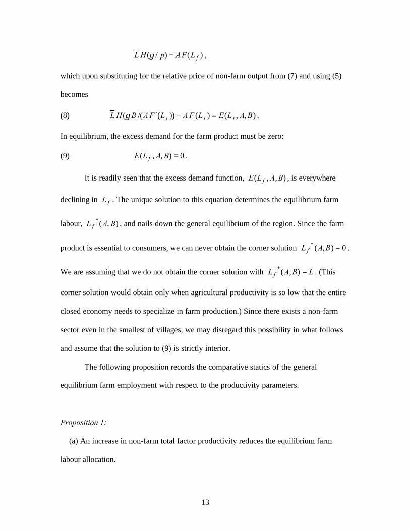
)()/( fLFApHL −γ ,

which upon substituting for the relative price of non-farm output from (7) and using (5)

becomes

(8) ),,()())(/(( BALELFALFABHL fff ≡−′γ .

In equilibrium, the excess demand for the farm product must be zero:

(9) 0),,( =BALE f .

It is readily seen that the excess demand function, ),,( BALE f , is everywhere

declining in fL . The unique solution to this equation determines the equilibrium farm

labour, ),(* BAL f , and nails down the general equilibrium of the region. Since the farm

product is essential to consumers, we can never obtain the corner solution 0),(* =BAL f .

We are assuming that we do not obtain the corner solution with LBAL f =),(* . (This

corner solution would obtain only when agricultural productivity is so low that the entire

closed economy needs to specialize in farm production.) Since there exists a non-farm

sector even in the smallest of villages, we may disregard this possibility in what follows

and assume that the solution to (9) is strictly interior.

The following proposition records the comparative statics of the general

equilibrium farm employment with respect to the productivity parameters.

Proposition 1:

(a) An increase in non-farm total factor productivity reduces the equilibrium farm

labour allocation.

14

(b) An increase in farm total factor productivity has an ambiguous effect on the

equilibrium farm labour allocation.

Proof:

(a) Totally differentiating (9) with respect to B, we obtain

(10) 0/),,()/](/),,([ *** =∂∂+∂∂ BBALEdBdLLBALE ffff .

From (8),

0)))(/()))((/((/),,( *** <′′′=∂∂ fff LFALFABHLBBALE γγ ,

where the inequality follows on using the fact that (.)H is decreasing in its argument.

Since the excess demand function is declining everywhere in fL , (10) yields the result

0/* <dBdL f .

(b) Totally differentiating (9) with respect to A, we obtain

(11) 0/),,()/](/),,([ *** =∂∂+∂∂ ABALEdAdLLBALE ffff .

From (8),

)()))(/()))((/((/),,( **2**ffff LFLFABLFABHLABALE −′−′′=∂∂ γγ .

Since the two terms on the right hand side of this expression are of opposite sign, we see

from (11) that the sign of dAdL f /* is ambiguous: an increase in A has an indeterminate

effect on equilibrium farm employment. �

The intuition for this result is as follows. Productivity increase, whether in the

farm or the non-farm sector, apart from obviously raising income, changes the relative

price of the non-farm good. When it is non-farm productivity that increases, at given

relative prices, the demand for farm output stays constant (with quasi-linear preferences)

15

while that for non-farm output increases. But, at the original labour allocation, the

relative price of non-farm output declines following the productivity increase, and this

induces consumers to curtail their consumption of farm output and substitute non-farm

output. The decline in demand for farm output releases labour from agriculture. In terms

of releasing labour from the farm sector, the income and substitution effects associated

with non-farm productivity increase work in the same direction. This explains part (a) of

the proposition.

When it is farm productivity that increases, at given relative prices, here too the

demand for farm output stays constant while that for non-farm output increases. But, at

the original labour allocation, the relative price of non-farm output increases following

the productivity increase, and this induces consumers to substitute away from non-farm

output and increase their demand for farm output. The increase in demand for farm

output raises the demand for labour in agriculture by working against the productivity

increase (which tends to release labour from the farm sector). In terms of releasing labour

from the farm sector, the income and substitution effects associated with farm

productivity increase work in opposite directions. This accounts for the ambiguous effect

of farm productivity increases on farm employment, as stated in part (b) of the

proposition.

The analysis above would seem to suggest that non-farm productivity increases

would be more efficacious than farm productivity increases in generating non-farm

employment. However, this would be an unwarranted conclusion: the relative effects of

the two productivity increases depend on the sensitivity of the consumer demand for farm

16

output with respect to the price of non-farm output—in other words, they depend on the

cross-price elasticity of farm output consumption.

To see this more clearly, we assume that the sub-utility function from farm output

consumption is given by

(12) 0,)( >−= − ααxxu ,

and the production function for this good is Cobb-Douglas:

(13) 10,)()( <<= δδff LALF ,

where δ represents the share of labour income in farm output. It is readily verified that,

in this case,

(14) )1/(1)/()/( αγαγ += ppH ,

which is an agent's consumption of the farm good when the solution to her utility

maximization problem is interior. The wage rate of a worker when fL workers are

employed in the farm sector is given by

(15) 1)( −= δδ fLAw .

The market clearing condition (9) for the farm good, which determines the

equilibrium farm employment, becomes

1/(1 ) ( 1)/(1 )( /( )) ( ) ( ) 0f fL A B L A Lα δ α δαδ γ + − + − = ,

the solution to which is

(16) )1/(1* )/(),( δαα += BACBAL f , where )1/(1)1/()1( )/()( δαδαα γαδ +++= LC .

The elasticity of equilibrium farm employment with respect to A and B are,

respectively, )1/( δαα +− and )1/(1 δα+− . Thus the absolute value of the elasticity of

17

farm employment with respect to farm productivity exceeds that with respect to non-farm

productivity if 1>α .

The parameter α is related to the cross-price elasticity, px,η , of farm output

demand with respect to the non-farm price. From (14), we see that )1/(1, αη +=px , so

that 1/1 , −= pxηα . The condition 1>α translates into the inequality 2/1, <pxη . Thus if

a 1% decline in the price of non-farm output curtails the demand for farm output by less

than 0.5%, the absolute value of the elasticity of farm employment with respect to farm

productivity would exceed that with respect to non-farm productivity. In the extreme case

of lexicographic preferences (zero substitutability in consumption between farm and non-

farm output, that is, 0, =pxη ), non-farm productivity improvements will release no

labour at all from agriculture [Eswaran and Kotwal (1993)]. For farm productivity

improvements to be more efficacious than non-farm productivity improvements in

removing labour from agriculture, the cross-price elasticity px,η has to be “sufficiently”

small. Since the demand for food is driven by the biological instinct for survival,

however, there would be very limited scope for substitution between farm and non-farm

output, especially at low levels of income.

Whether this is so or not is, of course, an empirical matter. Some evidence that

corroborates this hunch is found in Deaton (1997, Ch. 5, Table 5.7), which is drawn from

Deaton, Parikh, and Subramanian (1994). This Table presents the cross-price elasticities

of the demands for eleven food items with respect to nonfood goods for rural

Maharashtra for 1983. Many of these cross-price elasticity coefficients are insignificantly

different from zero. We aggregate all food items into a single ‘farm product’, and obtain

the imputed cross-price elasticity of this product with respect to the price of the nonfood

18

aggregate (using budget shares) and setting the statistically insignificant elasticities to be

zero. We obtain the figure of 0.11 as the cross-price elasticity for the aggregate good

denoting ‘farm’ product, which is much less than 0.5.

We can push this exercise a little further and investigate when the wage rate will

be more sensitive to productivity improvements in the farm sector than in the non-farm

sector. Substituting (16) into (15), the equilibrium wage rate may be written in terms of A

and B:

(17) )1/(1111 )( δαδαδδ +−+−= BACw .

We immediately see from (17) that the elasticity of the equilibrium wage rate with

respect to farm productivity is always higher than that with respect to non-farm

productivity (since 0>α for the assumed functional form). For more general functional

forms for (.)u , from what we have already argued, we would expect the difference

between these elasticities to be higher (in favour of farm productivity) the lower is the

cross-price elasticity, px,η . This is because low cross-price elasticities facilitate the

release of labour from the farm sector when the productivity in that sector increases,

reinforcing the wage increase brought about by the productivity improvement. This

prediction regarding the elasticities of farm employment with respect to farm and non-

farm productivities is eminently testable.

Region as a Small Open Economy

We briefly consider the other polar extreme, where each region is deemed a small

open economy. The prices of the outputs are assumed to be set at the all-India (or the

world) level. From the point of view of a single region, the relative price of non-farm

19

output is assumed to be fixed at some level p . We assume labour to be immobile across

regions. While there is labour migration in reality, especially from some specific regions

of India to others specific regions, at the country-level migration is small enough to

render labour immobility a reasonably good working assumption.

The consumers’ optimization problem is the same as that in the case of a closed

economy; only the market determination of the relative price of the non-farm sector

changes. For ease of comparative statics, we assume that the region does not completely

specialize; that is, there are always operational farm and non-farm sectors—however

small—within the region. 2 The equilibrium is easily nailed down: the equilibrating

condition is that the value of the marginal product of labour must be equated between the

farm and non-farm sectors. That is,

(18) BpLFA f =′ )( .

The comparative static derivatives of the equilibrium farm employment, ),(ˆ BAL f , are

trivially determined. We record this for ease of subsequent reference:

Proposition 2: When the region is a small open economy within the country,

(a) an increase in non-farm productivity decreases equilibrium farm employment,

(b) an increase in farm productivity increases equilibrium farm employment.

Proof: Immediate, on totally differentiating (18) with respect to the productivity

parameters and invoking strict concavity of the farm production function:

(a) 0/),(ˆ <dBBALd f , and (b) 0/),(ˆ >dABALd f .

20

Local consumer demand is irrelevant here since the region can import from and

export to other regions in the country. Higher total factor productivity improves the

region's comparative advantage (or reduces the comparative disadvantage) in that sector

and more labour is absorbed into it as a result. The region will either export more of the

good to other regions or import less of it.

Parts (a) of Propositions 1 and 2 are identical, that is, whether the region is a

closed economy or a small open economy, an increase in non-farm productivity releases

labour from agriculture. However, since the result in the case of a closed economy is

ambiguous, parts (b) of the two propositions can be potentially different. [This result is

somewhat reminiscent of Matsuyama (1992) though, because he employs Stone-Geary

preferences, the effect of agricultural productivity increase in a closed economy is

unambiguous in his case, as it is in Eswaran and Kotwal (1993).] This difference opens

the door to possible empirical examination of which scenario is more appropriate as a

description of the typical region. In particular, if the data show that regions with higher

agricultural productivity employ less labour in the farm sector, all else constant, the

presumption that the regions are small open economies would be directly refuted. This

inference would be further corroborated if it is found that the elasticity of farm

employment with respect to farm productivity is not only of the same sign but also

greater in magnitude than that with respect to non-farm productivity. Such a finding, in

addition, would provide circumstantial evidence that the cross-price elasticity px,η is

small. For only then would the substitution effect associated with the relative price

2 Theoretically, complete specialization can never occur in the non-farm sector because the marginal

21

increase of the non-farm product following farm productivity improvements be

dominated by the income effect that induces agents to consume more non-farm output.

The comparative statics of the equilibrium wage rate with respect to the two

productivities present a stark contrast:

Proposition 3: When the region is a small open economy, the equilibrium wage rate has

(a) zero elasticity with respect to farm productivity, and

(b) unitary elasticity with respect to non-farm productivity.

The proof of this proposition is apparent from condition (18). As long as the

region has even a smallest of non-farm sectors, the value of the marginal product of

labour is pinned down by this sector. If farm productivity increases, this sector absorbs

more labour until the entire initial increase in the wage rate is dissipated: farm

productivity increases have zero effect on the equilibrium wage rate. Non-farm

productivity increases, on the other hand, increase the wage rate in proportion by drawing

out labour from the farm sector. This sharp difference in the predicted effects of the two

productivities on the wage rate arises from the fact that labour faces diminishing returns

in the farm sector (due to a fixed factor) but not in the non-farm sector. We could

introduce diminishing returns to labour even in the non-farm sector by, for example,

incorporating capital as an input (in both sectors) and having capital be a fixed factor in

the short run. In that case, both productivity increases would raise the wage rate—the

outflow of labour from a sector to the one experiencing the productivity increase would

product of labour is unbounded when farm output is zero; complete specialization, if it ever occurs, canoccur only in the farm sector.

22

raise the equilibrium value of the marginal product of labour (in both sectors). We would,

however, expect the equilibrium wage rate to be more elastic with respect to non-farm

than farm productivity as long as diminishing returns to labour is less constraining in the

non-farm sector.

Before we turn to investigating the empirical reality in India, we collect the

potentially testable empirical hypotheses drawn from the theory:

1. All else constant, farm productivity and farm employment should be positively

correlated if the regions approximate open economies within the country but could be

negatively correlated if the regions approximate closed economies. Lower farm

employment in regions with greater agricultural productivity would provide strong

evidence that regions are better treated as closed economies.

2. If the region is an open economy and there is incomplete specialization, the wage rate

would have lower elasticity with respect to farm than non-farm productivity. (With

complete specialization in the farm sector, productivity increase in the non-farm

sector would, of course, have no effect of the equilibrium wage rate.)

3. If the region is a closed economy, the agricultural wage rate will be more elastic with

respect to farm as opposed to non-farm productivity if the cross-price elasticity of the

demand for farm output with respect to the non-farm output price is sufficiently low.

5. Cross-sectional Analysis: Empirical Model and Data

Irrespective of whether the economy is closed or open, the theoretical model can

be reduced to two equations that determine wages and farm employment (using equations

(5) and (9) if the economy is closed or equations (5) and (18) if the economy is open).

23

The exogenous variables in these reduced form equations would be the total factor

productivities in the farm and non-farm sectors. The predictions of the earlier section

could then be examined by estimating the reduced form equations for regions in rural

India.

Data limitations, however, mean that such a relation cannot be estimated. The

ideal data set would contain repeated observations on the dependent and independent

variables for a number of years. As wages data are available only at five yearly intervals,

we do not have sufficient observations at the all India level or at the state level. The

difficulty is compounded by the absence of non-farm TFP data. Various estimates are

available for the organized manufacturing sector but only at the state level (for example,

Veeramani and Goldar (2004)). But this leaves out the unorganized manufacturing as

well as the entire service sector. It is the service sector expansion that has contributed

most to the growth of non-farm employment between 1983 and 1999. Therefore,

restricting the measure of non-farm TFP to manufacturing is unlikely to capture the

impact of non-farm TFP on non-farm employment and wages. The lack of relevant data

means that econometric analysis cannot shed light on the relative importance of

agricultural and non-agricultural TFP in explaining wage growth of agricultural labour.

However, analysis can still test some of the key predictions of the theoretical framework.

To resolve the problem of insufficient observations, we estimate the regressions at

the village level due to the two stage sampling design of the employment surveys where

the village is the primary sampling unit and the households are sampled from the selected

villages. For small geographical units, findings can be conclusive in only one direction.

If the findings indicate that agricultural TFP plays a dominant role in driving wages, then

24

the result can only be stronger for larger geographical aggregates. However, if non-

agricultural TFP is important in explaining wages, then this need not indicate a similar or

stronger result for larger geographical aggregates because the economy could be closed at

this level. The reduced form model can then be written as

(19) vvvvv uEBAf ++++= 3210 ββββ

(20) vvvvv EBAw εϕϕϕϕ ++++= 3210

where v indexes the village, f and w are the log of farm employment and wages

respectively, A and B are the log of total factor productivities in the farm and non-farm

sector respectively, and E controls for differences in village endowments (population,

irrigated land, cultivable land).

The agricultural wage and employment data is available from the all-India

employment surveys of the National Sample Surveys Organization (NSSO), where

households are the final sampling units and the survey reports the employment status of

each member of the household. In this paper we use that part of the schedule where, for

the reference period of a week, the survey elicits an individual’s time disposition during

each half-day of the week. This data takes into account multiple economic activities and

employment states that are characteristic of poor households. Furthermore, as

households are surveyed uniformly throughout the year, the aggregates derived from

weekly data are representative of annual aggregates. The NSS surveys are conducted at

5-year intervals and the unit level data from 1983, 1987-88, 1993-94 and 1999-00

surveys are available.

25

For the reference period of a week and for each economic activity reported by an

individual, the employment survey also reports the weekly earnings.3 A measure of

daily earnings in the activity can be obtained by dividing the weekly earnings by the

number of days worked in that particular activity. To control for cost of living

differences across time and across states, wages have to be deflated. The Planning

Commission uses the consumer price index for agricultural labourers and the consumer

price index for urban manual workers to update its poverty line in nominal values. We

use the deflator implicit in the Planning Commission poverty lines to deflate wages

across time and states.

While the dependent variables of (19) and (20) can be obtained from the NSSO

surveys, TFP estimates must be sought elsewhere. In the literature, estimates of farm

TFP are available only at the state level (Fan, Hazell and Thorat, 1999). One exception is

Kumar, Kumar and Mittal (2004) which contains estimates at the district level but they

confine their exercise to states in the Indo-Gangetic belt. To overcome this limitation, we

combine data on output and inputs from Bhalla and Singh (2001) with cost share

information from the cost of cultivation surveys. While the data in Bhalla and Singh is at

the district level, we construct TFP estimates at a higher level of aggregation. Over time

districts have been subdivided and new districts formed. To ensure comparability across

periods, Bhalla and Singh present their data according to the district boundaries in 1961.

It is therefore not possible to disaggregate their data so that it maps to district definitions

in the more recent NSS data. The sampling design of the NSS uses a larger geographical

area called the NSS region. The NSS region consists typically of more than one district

and its boundaries are usually those of its constituent districts. Since it is possible to

3 Earnings are not available for self-employed individuals.

26

aggregate the Bhalla and Singh data to the NSS region level in a consistent manner, we

are able to construct farm TFP estimates at the NSS region level. However, this data set

is confined to the crop sector and so are the cost shares from the cost of cultivation

surveys. Another limitation is that the Bhalla and Singh data is not available for the

period beyond 1993. Our analysis is therefore limited to 1983 and 1993-94.

The absence of non-farm TFP estimates has already been discussed. As estimates

of non-farm output are available only at the state level, it would be beyond any researcher

to obtain non-farm TFP measures at a lower level of geographical aggregation. However,

state level estimates would probably suffice as non-farm TFP is unlikely to be as

narrowly location specific as farm TFP. Economic policies, technology, and

infrastructure (the primary determinants of non-farm TFP) are likely to be uniform across

a well-defined political and administrative unit such as a state. If so, we could assume

that non-farm TFP is invariant within a state and use state-specific fixed effects to control

for non-farm TFP. This strategy allows us to consistently estimate the impact of farm

TFP on the endogenous variables; however, it cannot give us the impacts of non-farm

TFP. The version of (19) and (20) that is therefore estimated looks like the following.

(21) vrsvrssrsvrs uEAf ++++= 3210 ββββ

(22) vrsvrssrsvrs EAw εϕϕϕϕ ++++= 3210

where the variables are now indexed by the level of geographical aggregation. For

instance, while vrsf is the log of farm employment in village v of NSS region r and state

s, rsA is the farm TFP in region r of state s. Note that 2 sβ and s2ϕ are state fixed effects

and capture among other things the state specific non-farm TFP.

27

6. Cross-sectional Analysis: Findings

Our interest in the above regressions is the coefficient of farm TFP. In particular,

we would like to check the theoretical predictions that in a small open economy, farm

TFP has no impact on agricultural wages and that an increase in farm TFP leads to higher

farm employment.

In the benchmark case, the dependent variables are the log of mean farm wage in

the village and the log of the ratio of farm work days to all work days (farm + non-farm).

We use the latter variable rather than farm work days to control for labor supply response

to farm TFP. As farm TFP could have different impacts on males and females and also

on different age cohorts within males we also consider variants where we vary the group

of workers over which farm employment and wages are defined. Besides the distinction

between male and female workers, we also consider three age cohorts within males –

young males (aged between 18 and 33), middle aged males (between 34 and 49 years of

age) and older males (between 50 and 66 years). The control variables are the ratio of

village population to land, the proportion of cultivable land that is irrigated and dummy

variables for the quarter in which the household was surveyed. Variables measuring the

age composition and education profile of the village population were insignificant.

We first consider results from 1983 displayed in Table 1. The coefficient of farm

TFP in the wage regression is positive and significant. The elasticity is around 0.5 for all

the variants. For all workers, the elasticity of farm employment (normalized by total

work days) to farm TFP is –0.28 and is highly significant. For sub-groups of females and

young males, the impact is much larger. As can be seen, the only group of workers for

28

whom the impact of farm TFP is not well estimated are the older male workers. These

results contradict the predictions about the impact of TFP in a small open economy.

Table 2 displays the results from the employment and TFP data for 1993/94. The

coefficient of farm TFP in the wage regression remains positive and significant for all

groups of workers. However, it is about half of the magnitude in 1983. Thus, while the

result contradicts the extreme case of a small open economy, it also indicates a movement

since 1983 towards a small open economy. This is confirmed by the employment

regressions. The coefficient of farm TFP is positive but small and insignificant. Within

the sub-groups, the picture is no longer uniform. While female employment is still

negatively correlated with farm TFP (but the elasticity is less than half of what it was in

1983), the employment of young males is positively and significantly impacted by farm

TFP.

Closed and small open economies, of course, are polar extremes. The

econometric results suggest that villages are better thought of as intermediate between

these extremes – as “large” open economies – while villages trade with the outside world,

the prices they face are not independent of the volume of transactions. For villages that

are not well connected to markets (because of distance, for example), an increase in farm

output (due to higher productivity) might pose problems in marketing. As a result, farm

produce prices depend on the local output even when part of it is traded. Our cross-

sectional analysis above suggests that between 1983 and 1993, villages got more

integrated with larger markets, as a result of which they moved closer to being a small

open economy. Another striking result from the analysis is that the employment structure

of middle aged and especially older males is less responsive to farm TFP.

29

A larger unit than the village is the NSS region. We could estimate the wage and

employment regressions at the region level as well. As the data does not support the

view that even villages are small open economies, one would expect that this is even

more strongly contradicted at the region level. However, with only 57 regions and fixed

effects for the 15 states, the regressions are not as well estimated. The sizeable impact of

TFP on wages persists in the region-level regressions. The impacts on farm employment

are, however, not significant.

7. A Counter-factual: The Role of the Non-Farm Sector

While the previous section is suggestive of the role of agricultural productivity, it does

not pin down the contribution of non-farm economic growth to the rise in agricultural

earnings. Ideally, we would have liked to construct a panel across the time period

1983-99 to check how much of the variation in wage increases over the period could be

explained by productivity increases (TFP and inputs) in agriculture. But since we do

not have data on agricultural production in 1999, we have no alternative but to think of

a second best way to estimate the relative contribution of agricultural productivity

increases to wage increases in agriculture. We will call this second best alternative ‘a

counterfactual exercise’ to indicate the nature of the thought experiment involved in the

process.

Figure 2 is a graphical representation of the counterfactual that we wish to

consider. Here 1R and 1w denote, respectively, the agricultural labour-to-land ratio and

the wage rate (read off the marginal product curve) in 1983. In 1999, the marginal

product curve in agriculture shifts out, either because of greater use of other inputs or

30

because of an increase in total factor productivity. The new agricultural labour-to-land

ratio and wage rate are denoted by 2R and 2w , respectively. In the counterfactual,

suppose the non-farm sector didn’t create any additional jobs during 1983-99, so that

agriculture would have absorbed the additional employment that was created in reality

by the non-farm sector. The agricultural labour-to-land ratio would have increased to

HR2 and agricultural wages dropped to Hw2 . The distance between 2w and Hw2 is the

part of the observed wage increase ( 12 ww − ) that is due to the non-farm sector. Note

that this attributes the entire increase in non-farm employment to productivity increase

in the non-farm sector. This is surely not the case as a rise in agricultural productivity

leads to greater demand for non-farm goods and services and some part of non-farm

employment is due to it. In this sense, the procedure adopted in the counterfactual

overestimates the contribution of the non-farm sector and our estimate is an upper

bound.

The first column of numbers in Table 3 presents the proportional change in

agricultural employment if the non-farm sector had not created any jobs between 1983

and 1999.4 Note that there is considerable variation in the non-agricultural employment

created between 1983 and 1999 across states. Leaving aside the case of Kerala which is

an outlier (45% of total agricultural employment was created in the non-agricultural

sector between 1983 and 1999), the range of variation is from 10% in Orissa to 30% in

Punjab. It is noteworthy that the states that are well-known for having attracted

4 The proportional change in agricultural employment if the non-farm sector had not created any jobs

between 1983 and 1999 is given by NFEMPAGEMP

NFEMP∆+

∆, where NFEMP∆ is the change in non-farm

employment between 1983 and 1999 and AGEMP is agricultural employment in 1999.

31

relatively greater investment in the modern industrial sector (i.e., Gujarat, Haryana,

Karnataka, Maharashtra and Tamilnadu) have created considerable employment in their

non-farm sectors but no more than around 27%.

To take our thought experiment further, we need to be able to estimate how much

lower the change in labour earnings in agriculture would have been had the non-farm

sector created no additional jobs between 1983 and 1999. To answer this question, we

assume that the agricultural output, Q, is given by a Cobb-Douglas production function:

∏=

=n

ii

iXALQ1

ρδ with 1=+ ∑i

iρδ ,

where L denotes the amount of labor employed in agriculture, Xi denotes the ith input

other than labor (such as land, fertilizers etc), and A denotes the total factor productivity.

Let the period subscripts 1 and 2 denote variables in the years 1983 and 1999,

respectively. Denote by ),2,1(,,, =jwAXL jjijj the amount of agricultural labor used,

input Xi used, the total factor productivity, and the agricultural wage, respectively, in

period j. Taking the price of agricultural output as the numeraire, the wage rate in period

2 (given by the marginal product of labor) may be written

∏=

−−=n

ii

iXLAw1

2,)1(

222ρδδ = iLXA

n

ii

ρδ )/( 21

2,2∏=

Suppose l denotes the increase in non-farm employment over the 16 years under

consideration. Assume that if the non-farm sector had not created this employment, the

employment in agriculture in 1999 would have been higher by this amount. Let Hw2

denote the agricultural wage that would have prevailed in 1999 in this hypothetical

32

scenario. Assuming that all inputs other than labor would have been employed in this

fictitious setting at the same level that they were in 1999, we may write

ilLXAwn

ii

H ρδ ))/(( 21

2,22 += ∏=

= ii LlLXAn

ii

ρρδ −

=

+∏ )/1()/( 221

2,2 = in

iLlw ρ−

=∏ + )/1(

122 ,

which may be rewritten

(29) ∑−+= iLlwwH ρ)/1( 222 = )1(22 )/1( δ−−+ Llw

The observed increase in wages over the 16 years is 12 ww − . This increase can be

decomposed into that which would have obtained if the non-farm sector had not absorbed

any additional employment and the increase that came about because of additional non-

farm employment:

)()( 122212 wwwwww HH −+−=− .

The increase in wages that would have been observed in the hypothetical scenario, using

(29), is given by

(30) ])/1(1[ )1(2222

δ−−+−=− Llwww H .

From (30), we obtain the proportional increase in the agricultural wage

attributable to non-farm employment as:

(31) ])/1(1))[/(()/()( )1(21221222

δ−−+−−=−− Llwwwwwww H .

This expression is couched entirely in terms of observable quantities and can be readily

computed if we have an estimate ofδ .

In competitive markets, δ is equal to the output share of labor. National account

statistics do not provide data on the value of agricultural output. However, the value of

principal crops and the value of livestock is available state-wise and we consider their

33

sum to be the value of output from agriculture.5. Agricultural employment and average

daily wages in each state are computed from the NSS data. For rural areas the NSS data

also contains details about the type of operations the individual was working in. To

keep our estimates of agricultural employment and wages comparable with the value of

output data, we excluded work in forestry, fisheries and activities other than cultivation.

The share of labour in agriculture, then, is simply the ratio of the estimated wages paid

out to labour to the value of output in agriculture. These labour shares are displayed as

the third column in Table 3.

We evaluate the maximum possible increase in agricultural wages across all

workers that could be attributed to non-farm sectoral growth using the labor shares

appropriate for each state. This is done in Table 3. The second column of numbers

presents the observed ratio of average agricultural wages in 1999 to that in 1983 for the

15 major states.6 (These 15 states accounted for 98% agricultural employment in 1999.)

The all-India ratio (aggregate of 15 states) for agricultural earnings is shown at the

bottom of the column. Between 1983 and 1999, at the all India level agricultural wages

grew by 69%.

The fourth column of numbers in Table 3 shows the maximum projected

proportional change in agricultural earnings that could possibly be attributed to the

growth of the non-farm sector during 1983-99. It is computed using expression (31).

5 The data are collected from various issues of Value of Output from Agriculture and Livestock, CentralStatistical Organisation, Ministry of Statistics and Programme Implementation, Govt. of India. The cropsincluded are cereals, fruits and vegetables, total fibres, pulses, sugar, oilseeds, spices, total drugs andnarcotics, total by-products, indigo and other crops.6 Agricultural wages are approximated by average daily wages in agriculture. The daily time dispositionblock in the NSS employment rounds gives total weekly earnings and days worked in the week by activity.Average daily earnings are derived as the ratio of the two.

34

The fifth column shows the proportion of the observed increase that can be attributed to

the non-farm sector. So, for example, in the state of Andhra Pradesh the non-farm sector

was responsible for only 18.9% of the increase in real agricultural wages over the

period 1983-99. Assam is the only state where real agricultural earnings were almost

stagnant during this period. Without the growth of the non-farm sector in the state,

agricultural earnings would have fallen. In the final two columns of Table 3, we present

standard errors and the associated t-statistics for the contribution of the non-farm sector

presented in the fifth column. These standard errors are obtained by a cluster bootstrap

with a thousand replications.7 Other than for Assam, the contribution of the non-farm

sector is precisely estimated.

Ignoring Assam, where the estimates are not precise, the maximum contribution

of the non-farm sector varies from a low of 9% for Bihar to a high of 55% for Punjab.

States where the contribution of the non-farm sector is greater than 30% are

are Haryana, Kerala, Punjab and West Bengal. Other than Gujarat, Maharashtra and

UP, in all the other states the maximum impact of the non-farm sector is limited to less

than 20% of the earnings increase. The 15-state average at the bottom of the second

column is obtained by considering just the 15 states. Overall, therefore, growth in the

non-farm sector could at the most have accounted for 23% of the increase in agricultural

earnings between 1983 and 1999.

7 As noted earlier, the NSS surveys have a two stage design where clusters (villages in the rural sector andurban blocks in the urban sector) are sampled in the first stage and households from the selected clusters inthe second stage. There are 10527 clusters in the 1983 survey and 8530 in the 1999 survey (in our sampleof 15 states). The bootstrap draws 1000 samples of the clusters (with replacement) and the contribution ofthe non-farm sector is calculated for each sample. The standard error of this statistic is calculated from itsdistribution over all the samples.

35

In the above discussion, we have assumed that each state is a closed economy by

which we mean that the relative price between the farm and non-farm goods in each

state is determined completely by the demand and supply within the state. The

assumption is supported by the results of Section 6, at least till 1993. One way to think

about it is to think of the economy of a state as a ‘large’ open economy in a continuum

situated between two extremes: one where the size of the outside economy that the state

is trading with is negligibly small compared to the size of its own economy (closed),

and the other where its own size is negligibly small compared to the size of the external

economy with which it trades (open). As trading costs (including transportation costs)

fall and a state starts trading with wider and wider regions, it moves from the closed

economy end of the continuum towards the open economy end. Our assumption of a

closed economy for a state should not be regarded as an assertion that there are no trade

flows among Indian states but is tantamount to saying that Indian states are still close to

the first end of the continuum. As trading costs have fallen all over the country, many

states may have moved a little distance along the continuum. What does this mean for

the relative contribution we have attributed to the productivity increase in non-farm

sector?

As long as all states are close to the closed economy end, we can consider the

different positions they occupy on the continuum as the extent to which the relative

price of the non-farm good is different from the relative price that would obtain under a

closed economy. In other words, what we have designated as the upper bound on the

contribution of the productivity growth in the non-farm sector should be in fact

regarded as the upper bound on the combined contribution of the contribution of the

36

productivity growth in the non-farm sector plus the changes in relative price of the non-

farm good introduced by trade with the areas across the state borders. Viewed this way,

it is noticeable that a lion’s share of the increase in agricultural wages over the period

1983 -99 have resulted from an increase in agricultural productivity increase.

8. Conclusions

In this paper, we have attempted to assess the relative impacts of productivity growth in

the farm and non-farm sectors on India’s poverty (as proxied by the real wage). We set

out a theoretical model consistent with Engel’s Law and generate some theoretical

predictions on the wage and labour allocation effects of productivity growth in the two

sectors. Cross-sectional evidence from the 1983 and 1993 NSS rounds confirm the

predicted effects of farm TFP differences. Because of severe data limitations, however,

we are unable to identify the effects of non-farm TFP differences. To remedy this, we

then conduct a counterfactual exercise to evaluate the relative contributions of the farm

and non-farm sectors on the real wage increase in India between 1983 and 1999. We

find that, at the all-India level, the non-farm sector’s contribution is no greater than a

quarter.

37

References

Besley, T. and R. Burgess (2002), “The Political Economy of GovernmentResponsiveness: Theory and Evidence from India”, Quarterly Journal of Economics,117, pp. 1415-1452.

Besley, T. and R. Burgess (2003), “Halving Global Poverty”, Journal of EconomicPerspectives, Summer, 17, pp. 3-22.

Besley, T. and R. Burgess (2004), “Can Labor Regulation Hinder EconomicPerformance? Evidence from India”, Quarterly Journal of Economics, 119, pp. 91-134.

Besley, T., R. Burgess, and B. Esteve-Volart (2005), “Operationalizing Pro-Poor Growth:India case Study”, Department of Economics, London School of Economics.

Bhalla, G. S. and G. Singh, (2001), Indian Agriculture: Four Decades of Development,Sage: New Delhi.

Burgess, R. and R. Pande (2005), “Do Rural Banks Matter? Evidence from the IndianSocial Banking Experiment”, American Economic Review, 95, pp. 780-795.

Datt, G. and M. Ravallion (1998), “Farm Productivity and Rural Poverty in India”,FCND Discussion Paper No. 42, International Food Policy Research Institute,Washington D.C., www.ifpri.org/divs/fcnd/dp/papers/dp42.pdf

Datt, G., and M. Ravallion (2002), ‘Is India’s Economic Growth Leaving the PoorBehind?”, Journal of Economic Perspectives, 16(3), pp. 89-108.

Deaton, A. (1997), The Analysis of Household Surveys, Johns Hopkins University Press,Baltimore.

Deaton, A., (2005), “Prices and Poverty in India”, in A. Deaton and V. Kozel (eds.), TheGreat Indian Poverty Debate, New Delhi, India. MacMillian.

Deaton, A. and J. Dreze (2002), “Poverty and Inequality in India, a Reexamination”,Economic and Political Weekly, Sept 7, pp. 3729-48.

Deaton, A., and V. Kozel (2005), (Ed.,) The Great Indian Poverty Debate, Delhi:Macmillan India

Deaton, A., K. Parikh, and A. Subramanian (1994), “Food Demand Pattern and PricingPolicy in Maharashtra: An Analysis Using Household Level Survey Data”, Sarvekshana,17, pp. 11-34.

Deaton, A., and A. Tarozzi (2005), “Prices and Poverty in India”, in A. Deaton and V.Kozel (eds.), The Great Indian Poverty Debate, New Delhi, India. MacMillian.

38

Dollar, D., and A. Kraay (2002), “Growth is Good for the Poor”, Journal of EconomicGrowth, 7, pp. 195-225.

Eswaran, M. and A. Kotwal (1993), “A Theory of Real Wage Growth in LDCs”, Journalof Development Economics, 42, pp. 243-270.

Fan S., P. Hazell, and S. Thorat, Linkages between Government Spending, Growth andRural Poverty in India, Research Report 110, International Food Policy ResearchInstitute, Washington D.C.

Foster, A. and M. Rosenzweig (2003), “Agricultural Development, Industrialization, andRural Inequality”, Brown University, mimeo.

Foster, A. and M. Rosenzweig (2004), “Agricultural Productivity Growth, RuralEconomic Diversity and Economic Reforms: India 1970-2000”, Economic Developmentand Cultural Change, pp. 509-542.

Goldar, B. (June 2004), Productivity Trends in Indian Manufacturing in the Pre-and Post-Reform Periods, ICRIER Working Paper#137

Kijima, Y., and P. Lanjouw (2005), “Economic Diversification and Poverty in RuralIndia”, Indian Journal of Labour Economics, 48 (2): 349-374.

Kumar P., A. Kumar and S. Mittal (2004), “Total Factor Productivity of Crop Sector inthe Indo-Gangetic Plain of India: Sustainability Issues Revisited”, Indian EconomicReview, 39 (1): 169-201.

Lewis, W.A. (1954), “Economic Development with Unlimited Supplies of Labour”,Manchester School of Economic and Social Studies, 22, pp. 139-191.

Lopez (2004), “Pro-Poor Growth: A Review of What We Know (and of What WeDon’t)”, manuscript, World Bank, downloaded fromwww.nadel.ethz.ch/lehre/ppg_review.pdf

Kraay, A. (2004) “When is Growth pro-Poor? Evidence from a Panel of Countries”,World Bank.

Matsuyama, K. (1992), “Agricultural Productivity, Comparative Advantage, andEconomic Growth”, Journal of Economic Theory, 58, pp. 317-334.

Palmer-Jones, R. and K. Sen (2003), ‘What has luck got to do with it? A regional analysisof poverty and agricultural growth in India’, Journal of Development Studies, 2003,40(1): 1-31.

Ravallion, M. (2001), “Growth, Inequality, and Poverty: Looking Beyond Averages”,World Development, 29 (11): 1803-1815.

39

Ravallion, M. and G. Datt (1996), “How Important to India’s Poor is the SectoralComposition of Economic Growth”, World Bank Economic Review, 10(1), pp. 1-25.

Topalova, P. (2005), “Trade Liberalization, Poverty and Inequality: Evidence from IndianDistricts”, Department of Economics, Massachusetts Institute of Technology, August.

Veeramani C. and B. Goldar (2004), “Investment Climate and Total Factor Productivityin Manufacturing: Analysis of Indian States”, Working Paper No. 127, Indian Council forResearch on International Economic Relations, New Delhi.

40

Figure 1: Real (daily) Wages in Agriculture and Labour-Land Ratio

PunjabHaryana

Rajasthan

MH

Gujarat

Kerala

OrissaKarnatakaMP

Assam

UPWBAP

Tamil NaduBihar

Haryana

Punjab

Kerala

Rajasthan

GujaratMHAssam

Orissa

Karnataka

MP

UPWB

Tamil Nadu

AP

Bihar

20

40

60

80

Re

al D

aily

Wa

ge

100 200 300 400 500 600Labour-Land Ratio

wage83 wage99

41

Table 1: Coefficient of log of farm TFP, 1983

Dependent VariableGroup of workersover which thedependent variableis defined

Log of Mean wages Log of ratio of farm work daysto total work days

N Coefficient p-value N Coefficient p-valueAll 5792 0.56 0 6778 -0.28 0Males 5614 0.53 0 6778 -0.25 0.002Females 3687 0.53 0 6778 -0.62 0Young Males 4472 0.48 0 6778 -0.60 0Middle AgedMales

38170.47 0

6778-0.57 0

Older Males 2204 0.50 0 6778 -0.20 0.145Control variables are the ratio of population to land in the village, the proportion of land irrigated and statefixed effects

Table 2: Coefficient of log of farm TFP, 1993

Dependent VariableGroup of workersover which thedependent variableis defined

Log of Mean wages Log of ratio of farm work days tototal work days

N Coefficient p-value N Coefficient p-valueAll 4969 0.26 0 5868 30.06 0.193Males 4783 0.24 0 5868 0.10 0.035Females 3143 0.16 0 5868 -0.23 0.006Young Males 3704 0.18 0 5868 0.25 0.003Middle AgedMales

33240.21 0

58680.09 0.308

Older Males 1959 0.20 0.002 5868 0.10 0.26Control variables are the ratio of population to land in the village, the proportion of land irrigated and statefixed effects

42

Table 3: The Relative Contribution of the Non-farm Sector to Wage Increases

State Proportionalchangein agriculturalemployment(hypothetical)

Proportionalchange inagriculturalwages (actual)

LabourSharein valueofoutput in1999

Proportionalchange inagriculturalwagesdue tonon-farmsector

Proportionalcontributionof non-farmsectorto change inagriculturalwages

StandardError byBootstrap

t-statisticfor thecontributionof the non-farm sector

1

12 )(w

ww − δ

1

22 )(w

ww H−)()(

12

22

wwww H

−−

Andhra Pradesh 0.185 0.720 0.516 0.136 0.189 0.024 7.898Assam 0.283 0.055 0.484 0.127 2.293 114.101 0.020Bihar 0.118 0.691 0.670 0.061 0.089 0.018 4.895Gujarat 0.213 0.420 0.568 0.114 0.270 0.066 4.127Haryana 0.215 0.651 0.321 0.205 0.315 0.156 2.022Karnataka 0.148 0.966 0.426 0.149 0.155 0.034 4.544Kerala 0.445 0.732 0.397 0.345 0.471 0.045 10.575Madhya Pradesh 0.106 0.656 0.473 0.086 0.131 0.026 5.007Maharashtra 0.265 0.961 0.426 0.248 0.258 0.037 6.912Orissa 0.100 0.699 0.479 0.082 0.118 0.044 2.687Punjab 0.300 0.458 0.269 0.255 0.556 0.096 5.791Rajasthan 0.188 0.541 0.602 0.102 0.189 0.065 2.924Tamilnadu 0.271 1.364 0.574 0.230 0.169 0.025 6.671Uttar Pradesh 0.202 0.684 0.502 0.148 0.216 0.028 7.673West Bengal 0.244 0.537 0.323 0.212 0.394 0.075 5.224

0.198 0.685 0.461 0.156 0.228 0.010 21.935All India(15 States)

43

Wage Rate

Figure 2

Labour-Land Ratio, R

1983

1999

w1

w2

w2H

R1 R2 R2H