Youth poverty in Europe

Youth poverty in Europe

Maria Iacovou and Arnstein Aassve

This research examines poverty among young people aged 16 to 29, across 13 countries of the pre-enlargement European Union. Although young adulthood is known to be a time of uncertainty and vulnerability, there has been little research into the incidence of poverty among young people. This report aims to fi ll this knowledge gap.

More life-changing transitions occur during the young adult years than at any other time in people’s lives. This research looks at how these affect young people’s risks of poverty, including events such as:

n leaving the parental home

n setting up home with a partner

n fi nishing education

n fi nding (or not fi nding) a job, and

n starting a family.

The research compares young people’s experiences of poverty in the UK with those of peers in twelve other European countries. The authors identify those policies which best protect young people against poverty, and make a set of policy recommendations for the UK.

This publication can be provided in other formats, such as large print, Braille and audio. Please contact:Communications, Joseph Rowntree Foundation, The Homestead, 40 Water End, York YO30 6WP. Tel: 01904 615905. Email: [email protected]


Maria Iacovou and Arnstein Aassve

In association with Maria Davia, Letizia Mencarini, Stefano Mazzucco, Daria Mendola and Annalisa Busetta

The Joseph Rowntree Foundation has supported this project as part of its programme of research and innovative development projects, which it hopes will be of value to policymakers, practitioners and service users. The facts presented and views expressed in this report are, however, those of the authors and not necessarily those of the Foundation.

Joseph Rowntree FoundationThe Homestead40 Water EndYork YO30 6WPWebsite: www.jrf.org.uk

About the authorsMaria Iacovou and Arntein Aassve are Chief Research Ofi icers at the Institute of Social and Economic Research (ISER).

© University of Essex, 2007

First published 2007 by the Joseph Rowntree Foundation

All rights reserved. Reproduction of this report by photocopying or electronic means for non-commercial purposes is permitted. Otherwise, no part of this report may be reproduced, adapted, stored in a retrieval system or transmitted by any means, electronic, mechanical, photocopying, or otherwise without the prior written permission of the Joseph Rowntree Foundation.

ISBN: 978 1 85935 611 1

A CIP catalogue record for this report is available from the British Library.

Prepared by:York Publishing Services Ltd64 Hallfi eld RoadLayerthorpeYork YO31 7ZQTel: 01904 430033; Fax: 01904 430868; Website: www.yps-publishing.co.uk

Further copies of this report, or any other JRF publication, can be obtained from the JRF website (www.jrf.org.uk/bookshop/).

Contents

List of fi gures and tables vii

Acknowledgements ix

Summary x

1 Introduction 1

2 Data: the European Household Panel Survey (ECHP) 5

3 Key concepts 7A defi nition of ‘youth’ 7Income poverty 8Income in the ECHP 9Deprivation indices 10Welfare state typologies 11

4 Overview of youth poverty in Europe 13Patterns of poverty among young people in Europe 14Summary 26

5 How long do people stay poor? Poverty persistence and poverty recurrence 28

Poverty persistence 28The poverty ‘hit rate’ 31

6 What factors are associated with being poor? 34Results 34Summary 38

7 Entering and exiting poverty 39Controls 39Entering poverty 40Leaving poverty 42Summary 46

8 Does leaving home make you poor? 48Understanding causality 49Results 49Destination on leaving home 52Summary 54

9 Conclusions 55

Notes 57

References 60

Appendix A: Variables used for calculating deprivation index 65

Appendix B: Statistical methods used in Chapter 6 66

Appendix C: Statistical methods used in Chapter 7 70

Appendix D: Propensity Score Matching 77

vii

List of fi gures and tables

Figure 1 Poverty rates in the UK, Ireland and the social democratic countries 15

Figure 2 Poverty rates in the UK and the conservative countries 16

Figure 3 Poverty rates in the UK and the southern European countries 16

Table 1 Poverty rates by country, for three age groups and whole population 17

Figure 4 Percentage of young people who have left home, by age group and country 18

Figure 5 Poverty rates by whether young people live with their parents 19

Figure 6 Differences in poverty rates between those who have and have not left home, by the proportion of young people who have left home (those aged 20–24) 21

Figure 7 Poverty rates of 20–24-year-olds by household composition 22

Figure 8 Poverty rates by presence of children 24

Figure 9 Poverty rates by activity status 25

Figure 10 Poverty rates and poverty persistence for three age groups 29

Figure 11 Poverty ‘hit rates’ 32

Figure 12 Results from regressions estimating poverty and deprivation: marginal effects 35

Figure 13 Marginal effects from regressions estimating poverty entry 40

Figure 14 Marginal effects from regressions estimating poverty exit 44

Figure 15 The extra risk of entering poverty associated with leaving home: descriptive and PSM estimates 50

Figure 16 Increase in monetary deprivation scores associated with leaving home: descriptive and PSM estimates 52

Figure 17 Increase in non-monetary deprivation scores associated with leaving home: descriptive and PSM estimates 52

Figure 18 PSM estimates by destination on leaving home 53

Table B1 Descriptive statistics 67


Table B2 Random effects probit regression, dependent variable is poverty status based on 60 per cent of median net equivalised household income 68

Table B3 Random effects linear regression of total deprivation index 69

Table C1 Descriptive statistics, sample of those who are not poor and may enter into poverty 71

Table C2 Descriptive statistics, sample of those who are poor and may exit poverty 72

Table C3 Logit regression, with dependent variable: entering into poverty in the following year 73

Table C4 Logit regression, with dependent variable: exiting poverty in the following year 75

Table D1 ATT for those who leave home compared with stayers 79

Table D2 Indicators of covariance balancing, before and after matching 80

Table D3 Sample sizes 81

viii

ix

Acknowledgements

We are grateful to Helen Barnard and Chris Goulden of the Joseph Rowntree foundation, who acted as our research liaison offi cers.

We should also like to thank our advisory committee: Paul Gregg (Bristol University), Simon Burgess (Bristol University), Jackie Scott (Cambridge University), Elaine Squires (Department for Work and Pensions) and Simon Lunn (HM Treasury) for their support and feedback.

This research has been presented in several places, and is much improved as a result: thanks are due to those who commented on our work at presentations at ISER, the Centre for European Labour Market Studies at Gothenburg University, the EPUNET conference 2005, and the Centre for Advanced Studies in Oslo, and anonymous referees for Demographic Research and the European Journal of Population.

The work on poverty durations, and some of the analysis for the other chapters, was carried out by our collaborators during visits to ECASS (European Centre of Analysis in the Social Science), supported by the EU’s Access to Research Infrastructure action; and to IRISS at CEPS/Instead in Differdange, supported by the EU’s Research Infrastructures Action (Trans-national Access contract RITA 026040).

The ECHP data used in the analysis were produced and made available by Eurostat.

Any errors and inconsistencies in the report are our own.

x

Summary

Background

Young adulthood is a stage of life where individuals embark on a number of wide-ranging changes (leaving home, fi nding a job, setting up home with a partner and becoming parents). Many of these changes are potentially risky and stressful. Several areas of risk are relatively well documented as they relate to young people, but very little has been written to date about the economic stresses which young people face, and the associated risks of poverty and deprivation. The research in this report seeks to fi ll this gap in the literature by documenting the extent of poverty among young people across the pre-enlargement European Union, and analysing which young people are particularly at risk.

This report takes a comparative approach, studying cross-national differences in the incidence of poverty and deprivation. By taking this approach, we are able to assess how young people in the UK fare compared with their European peers; to ask whether certain policy regimes do better than others at keeping young people out of poverty; and to assess whether there are lessons for UK policy makers.

Our analysis takes a relatively broad defi nition of ‘youth’, covering young people aged 16–29; however, we often focus on smaller subgroups within this age range when it is appropriate to do so.

Data

All the analysis in this report is based on data from the European Community Household Panel (ECHP), a set of comparable large-scale longitudinal studies set up and funded by the European Union. The fi rst wave of the ECHP was collected in 1994 for the original countries in the survey: Germany, Denmark, the Netherlands, Belgium, Luxembourg, France, the UK, Ireland, Italy, Greece, Spain and Portugal. Three countries were late joiners to the project: Austria joined in 1995, Finland in 1996 and Sweden in 1997; the fi nal wave of the ECHP was collected in 2001. More information about the ECHP may be found in Chapter 2 of the report.

Summary

xi

Key concepts

This study focuses on three aspects of disadvantage.

Income poverty is a standard measure of poverty, defi ned as living in a household where the income (adjusted for household size) is lower than 60 per cent of median (average) household income in the country in which one lives.

Monetary deprivation is also based on income but, whereas poverty is a dichotomous variable (one is either poor or not poor), monetary deprivation is a continuous measure, ranging from the value 1 for those at the very top of the income distribution, down to 0 for those at the bottom.

Non-monetary deprivation is an index generated from 24 separate variables falling into fi ve categories: the inability to afford the basic requirements of life; the inability to afford a range of consumer durables; the lack of certain domestic facilities; other problems with one’s home; and problems with the neighbourhood in which one lives.

These indices are described in more detail in Chapter 3 of the report.

Overview of youth poverty in Europe

In Chapter 4, we measure the extent of youth poverty across 13 countries, broken down by age, family structure and employment status.

We show that youth poverty rates vary greatly across Europe: among the 20–24 age group, they vary from 8 per cent in Austria to 30 per cent in Finland.

Although in most countries young people are at higher risk of poverty than the population as a whole, this is not universally true: in Austria young people face a lower risk of poverty than the population in general, and young people also fare relatively well in Germany and Belgium. We attribute part of the success of Austria and Germany to their comprehensive systems of apprenticeships for young adults, which provide moderate incomes to young people as well as training opportunities.

The highest risk of youth poverty is found in Italy (where poverty rates are high across all age groups); but also in the Scandinavian countries and the Netherlands (where poverty rates among other age groups are extremely low). We attribute the very high youth poverty rates in this ‘social democratic’ group of countries to the very


xii

young age at which people leave the parental home in these countries; we return to this theme repeatedly during this report.

In the UK, youth poverty rates are fairly high, standing at 20 per cent for those aged 20–24: again, this appears to be associated with relatively early home-leaving in this country.

How long do people stay poor? Poverty persistence and poverty recurrence

In Chapter 6, we ask how long young people who have become poor are likely to stay poor. Across Europe, between 60 and 70 per cent of young people who are poor in one year will remain poor until the next year; this measure of poverty persistence does not vary a great deal between countries or by age group. Looking at poverty persistence in the longer term, young Italians fare worst: in the 16–19 age group, over two in fi ve of those who are poor in one year will still be poor two years later, and almost one in fi ve will still be poor four years later. Long-term poverty is also a concern in the UK, particularly among the older age group: of those aged 25–29 who are experiencing a spell of poverty, 73 per cent (almost three-quarters) will still be poor next year, while 16 per cent (almost one in six) will remain poor every single year for the next four years.

As an alternative defi nition of poverty persistence, we defi ne the poverty ‘hit rate’ – the proportion of years in which a young person is poor, ranging from 0 (never poor) to 100 per cent (constantly poor). Austria does particularly well on this measure, with the highest percentage of young people in the ‘never poor’ category, and the lowest number in the ‘constantly poor’ category. Italy does the worst, with around one in ten young people classifi ed as ‘constantly poor’; Finland does very nearly as badly.

What factors are associated with being poor?

In Chapter 6, we identify four factors associated with poverty and deprivation: living away from the parental home; living alone; having children; and not having a job.

All these factors have an effect but, in all countries except for the southern European countries plus Ireland, the picture is dominated by living away from the parental home. In the UK and France, plus the ‘social democratic’ countries, leaving home is associated with a hugely elevated risk of poverty, while in Germany, Austria and Belgium, the associated risk is more modest, but still outweighs all the other factors.

Summary

Being married or cohabiting tends to reduce the risks of poverty and deprivation, while having children is usually associated with a modestly increased risk. Interestingly, there is no extra risk associated with having children in the Scandinavian countries; the extra risk of poverty associated with having children is at its highest in the UK, at 10 percentage points.

While one might expect employment to play a highly signifi cant role in keeping young people out of poverty, our research shows that, in most countries, this role is very modest – particularly in relation to the family-based factors discussed above. One explanation for this may be that youth wages are relatively low; an alternative explanation, which we explore in the following chapter, may be that the crucial factor is not whether one has a job, but whether one is able to hold a job for a reasonable length of time.

Entering and exiting poverty

In Chapter 7, we examine the role of the same four factors as before: living away from the parental home; living alone; having children; and not having a job. However, we extend the analysis to look at how these factors change: for example, what happens not just when one lives away from home, but in the year when one moves?

As before, we fi nd that the most important factor is whether or not one lives with one’s parents: in all countries except for Southern Europe and Ireland, this single factor outweighs all the other factors. In addition, we fi nd that, in many countries (including the UK), there is a sizeable extra risk of poverty associated with having left home in the past year. It is very clear that young people are particularly vulnerable to poverty in the fi rst year of leaving home, and we feel there may therefore be a case for directing economic support towards young people at this time.

As before, we fi nd that being married or cohabiting reduces the deleterious effect of living away from the parental home: however, possibly because of costs associated with setting up a shared home, this effect is not manifested in the fi rst year of the relationship, which again underlines the case for support at this time.

Finally in this chapter, we examine the effects of having a job and keeping a job. We fi nd that, in most countries, it takes more than one year for the effects of employment to be realised: in other words, having a job does play a role in keeping young people out of poverty, but only in the longer term – in the shorter term, employment seems to have very little effect at protecting young people from poverty. This has

xiii


clear implications for social policy: job creation schemes for young people must be formulated with the longer term in mind, and their success must be measured against a time frame of one year or more.

Does leaving home make you poor?

In many places, this report has highlighted the enormous increase in economic risks associated with leaving home. However, the analysis in other chapters does not allow us to say for certain whether leaving home ‘causes’ young people to be poor, since it may be that young people who were at higher risk of being poor anyway are the ones who leave home earlier. In Chapter 8, we use an analytical tool known as Propensity Score Matching to deal with this problem and to attempt to establish whether there really is a causal effect for leaving home. We fi nd that there is a causal effect: if anything, the analysis in the previous sections slightly underestimates the effect of leaving home on youth poverty.

Conclusions

We identify four areas for policymakers to consider:

1 Leaving home is associated with a hugely increased risk of poverty, particularly in the fi rst year. There may be a case for providing fi nancial support for young people at this time.

2 Having a job is associated with a reduced risk of poverty for young people, but only if the job is held for longer than a year. Thus, employment schemes targeted at young people should aim to provide jobs for a year at least; and the success of such schemes should be evaluated over a time scale of at least one year.

3 Parenthood among young people in the UK is associated with the highest level of disadvantage anywhere in Europe, while the Scandinavian countries demonstrate that there need not be any disadvantage associated with parenthood.

4 As well as providing comprehensive and good-quality vocational training, the apprenticeship systems which operate in Austria and Germany appear to play a successful role in keeping young people out of poverty. This may be an important factor for those involved in considering the role of vocational training in the UK.

xiv

1

1 Introduction

This study focuses on poverty among young people in the pre-enlargement European Union. We examine the incidence of poverty among those aged 16–29 (focusing at times on smaller subgroups within this age range) and how this incidence varies between countries. We also investigate the characteristics and life events which are associated with poverty, how the effects of these factors vary between countries, and whether these comparisons highlight areas of interest for UK policy makers.

Over the last decade, a considerable amount of research has focused on the transition to adulthood, which may best be understood as the combination of many different transitions: completing one’s education, fi nding a job (and, in time, a stable and well-paid job), moving out of the parental home, moving in with a partner, and perhaps starting a family.

In the 1950s and the decades immediately following, the transition to adulthood tended to occur in a reasonably ordered and predictable fashion, with all the constituent transitions taking place over the space of only a few years. However, the last decades of the twentieth century and the start of the twenty-fi rst century have seen the transition to adulthood in many countries becoming more complex and protracted – often in ways which leave young people particularly vulnerable. With increasing levels of participation in higher education, young people are spending longer dependent on the state or their families for fi nancial support, and without earned incomes of their own. Additionally, changes to youth labour markets over recent decades mean that, when young people do enter the labour market, they may spend considerable periods without a job (Hammer, 2003; Russell and O’Connell, 2001) or in low-waged or insecure employment. Young people are also vulnerable in other areas, being more likely than those in other age groups to experience problems with housing (Rugg, 1999), drug abuse (Boys et al., 2001), and mental health problems (Shucksmith and Spratt, 2002). The mid-to-late teens and early twenties are also the years in which individuals are most likely to commit crimes and be incarcerated (Hansen, 2003).

That young adulthood is a time of heightened vulnerability in many dimensions is beyond doubt. However, whereas a great deal of research exists into several of these dimensions, very little has been written to date on how the often precarious situation of young people maps onto their economic situation, and the degree of poverty they experience. This lack of research on poverty among young people is particularly striking when viewed against the relatively large body of research on poverty among

2


other age groups at high risk – particularly children, among whom poverty, and the later effects of poverty, have been comprehensively documented (Bradbury and Jäntti, 1999; Cantillon and Van den Bosch, 2003; and many others).

For individuals at the very start of the transition to adulthood, the factors associated with youth poverty are similar to the factors associated with child poverty. The majority have no incomes of their own, and their risk of poverty is thus largely dependent on the incomes of adult members of their households (mainly their parents) in relation to the size of their households.

However, as young people move towards adulthood, the factors associated with youth poverty become more complex. Young people’s incomes vary widely – both between countries and within countries. Young people may be in education; they may have a job (low waged or better paid); they may be unemployed; they may be caring for children; or they may be out of the labour market for other reasons. The proportions of young people in each of these situations vary between countries, and the incomes associated with each situation vary between countries and also within each country. Young people’s living arrangements also vary – and again, this variation is observed both within and between countries. Many young people live with their family of origin (by which we mean their parents, plus any siblings still living at home). Others have left home and live alone or with a partner or with friends. Some have children of their own, with or without a partner. For young people with low or no earnings, living with their parents may protect them against poverty – although, conversely, the extra burden their presence places on household fi nances may throw the whole household into poverty. Alternatively, young people whose own earnings are relatively high may not be poor if they live apart from their families of origin and, if they do live at home, they may act as a resource for their families of origin (Cantó-Sanchéz and Mercader-Prats, 1999).

The relatively small literature which does exist on youth poverty suggests that it is an area worthy of research. The European Commission report on poverty (Eurostat, 2002) fi nds that, across Europe, the incomes of young people below age 24 are below national averages: the only groups poorer than young people are children and older people over age 65. Young people are also at higher risk than older groups of non-monetary deprivation (for example, living in substandard housing or lacking basic consumer durables) – though in this case the differentials between young people and other groups are less marked.

Iacovou and Berthoud (2001) fi nd that various factors – being in employment, having a working partner and living in one’s family of origin – protect young people against poverty, and that the risk of poverty is highest for those people for whom none of

3

Introduction

these protective factors is present. Young people in the Scandinavian countries are most likely to have no protective factors present, and most likely to be poor given the absence of protective factors.

Kangas and Palme (2000) study variations in poverty rates over the life cycle in eight OECD countries, considering a life-stage typology, based on four groups: ‘youth’, ‘family’, ‘empty nest’ and ‘old age’. Those who are childless young adults, under 25, are defi ned as ‘youth’, and this group is found to be at relatively high risk of poverty.

Smeeding and Ross Phillips (2002) analyse the economic suffi ciency of young people’s earnings in seven countries (France, Germany, Italy, Sweden, the UK, the US and the Netherlands). They fi nd that in all countries, only a minority of young people of either sex in their late teens and early twenties are able to support themselves with their earnings alone. Even when state welfare benefi ts are taken into account, a signifi cant proportion of young people remain unable to support themselves – and much less a family – before their mid- to-late twenties. Although young people’s incomes become markedly more suffi cient for their needs through the early twenties, poverty rates decline much more slowly over this age group, indicating that young people with low earnings are protected from poverty to a degree because of living with their families of origin.

Using data from the 1999 Poverty and Social Exclusion Survey of Britain, Fahmy (2002) fi nds that, on a range of fi ve poverty measures, those aged 16–24 are more likely to be poor than those aged 25–34. Thirty-three per cent of those in the 16–24 age group were poor, compared with only 16 per cent of those aged 25–34 years.

All of these studies highlight young adulthood as a time of heightened economic risk; however, with the partial exception of Iacovou and Berthoud (2001), they focus on describing youth poverty rather than explaining it. The research carried out for this report is a fi rst attempt to fi ll this gap in our knowledge.

This report is structured as follows.

Chapter 2 describes the data used for our analysis: the ECHP.

Chapter 3 defi nes a number of key concepts which we use throughout our research.

Chapter 4 describes how youth poverty rates vary between countries, and how poverty is related to factors such as having a job, having children and living away from the parental home.

4


Chapter 5 analyses poverty durations: given that some young people become poor, how long are they likely to remain poor?

Chapter 6 investigates the factors related to youth poverty in more detail, assessing the effects of a range of situations and events on the risks of poverty and deprivation.

Chapter 7 turns the focus to movements into and out of poverty, and examines the factors associated with these movements.

Chapter 8 performs a causal analysis of the relationship between being poor and leaving the parental home, asking whether being poor makes you leave home, or whether leaving home makes you poor.

There is no chapter in this report devoted to statistical methods. Different methods are used in each chapter; they are described briefl y in the relevant chapters, and references given for the reader who wishes to access a more in-depth description.

5

2 Data: the European Household Panel Survey (ECHP)

All the analysis in this report is based on data from the ECHP, a set of comparable large-scale longitudinal studies set up and funded by the European Union. The fi rst wave of the ECHP was collected in 1994 for the original countries in the survey: Germany, Denmark, the Netherlands, Belgium, Luxembourg, France, the UK, Ireland, Italy, Greece, Spain and Portugal. Three countries were late joiners to the project: Austria joined in 1995, Finland in 1996 and Sweden in 1997. The ECHP was terminated in 2001: thus, eight years’ worth of data are available for the majority of countries, and correspondingly fewer for the late joiners.

The ECHP has several advantages for the type of research that we undertake in this project. It is a large survey, and therefore enables meaningful inferences to be drawn at a country level. It is an ‘input harmonised’ survey: as far as possible, questions were harmonised (that is, designed to have comparable meanings and to generate comparable results) at the stage when the questionnaires were designed. This makes comparisons between countries possible in a way which is very diffi cult if several single-country surveys are considered.

Because it is a household survey, it collects data on all members of sample households. Thus, for all the young people who form our population of interest, we have information not just on the young people themselves, but on all the other adults who live in their households. We also have some data on children who live in those households: although this is of a relatively limited nature, it is suffi cient to draw many of the necessary inferences about household resources.

In addition, the longitudinal nature of the data (i.e. the fact that interviewers return year after year to the same individuals) is an important advantage, meaning that we are able to study not only people’s situation at a point in time, but also how individuals’ lives evolve over time: here, we are able to study not only who is poor, but who becomes poor, or who stops being poor.

Of course, there are some disadvantages with any data set. As far as this study is concerned, one major shortcoming of the ECHP is that, for young people who had left home by their fi rst interview, no information on their families of origin is available. For more information on the general quality of the ECHP, see Peracchi (2002) and Nicoletti and Peracchi (2005).

6


Additionally, data problems meant that we were unable to use data for two countries: Luxembourg, because the sample size was too small; and Sweden, because the Swedish data are not longitudinal.

Another diffi culty was posed by the ECHP income data. We discuss this diffi culty, and the strategy used to overcome it, in the next chapter.

7

3 Key concepts

A defi nition of ‘youth’

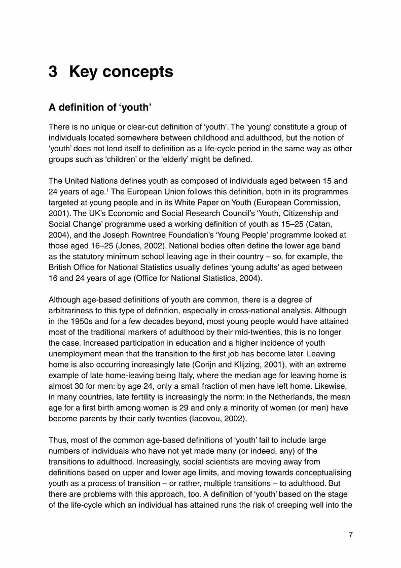
There is no unique or clear-cut defi nition of ‘youth’. The ‘young’ constitute a group of individuals located somewhere between childhood and adulthood, but the notion of ‘youth’ does not lend itself to defi nition as a life-cycle period in the same way as other groups such as ‘children’ or the ‘elderly’ might be defi ned.

The United Nations defi nes youth as composed of individuals aged between 15 and 24 years of age.1 The European Union follows this defi nition, both in its programmes targeted at young people and in its White Paper on Youth (European Commission, 2001). The UK’s Economic and Social Research Council’s ‘Youth, Citizenship and Social Change’ programme used a working defi nition of youth as 15–25 (Catan, 2004), and the Joseph Rowntree Foundation’s ‘Young People’ programme looked at those aged 16–25 (Jones, 2002). National bodies often defi ne the lower age band as the statutory minimum school leaving age in their country – so, for example, the British Offi ce for National Statistics usually defi nes ‘young adults’ as aged between 16 and 24 years of age (Offi ce for National Statistics, 2004).

Although age-based defi nitions of youth are common, there is a degree of arbitrariness to this type of defi nition, especially in cross-national analysis. Although in the 1950s and for a few decades beyond, most young people would have attained most of the traditional markers of adulthood by their mid-twenties, this is no longer the case. Increased participation in education and a higher incidence of youth unemployment mean that the transition to the fi rst job has become later. Leaving home is also occurring increasingly late (Corijn and Klijzing, 2001), with an extreme example of late home-leaving being Italy, where the median age for leaving home is almost 30 for men: by age 24, only a small fraction of men have left home. Likewise, in many countries, late fertility is increasingly the norm: in the Netherlands, the mean age for a fi rst birth among women is 29 and only a minority of women (or men) have become parents by their early twenties (Iacovou, 2002).

Thus, most of the common age-based defi nitions of ‘youth’ fail to include large numbers of individuals who have not yet made many (or indeed, any) of the transitions to adulthood. Increasingly, social scientists are moving away from defi nitions based on upper and lower age limits, and moving towards conceptualising youth as a process of transition – or rather, multiple transitions – to adulthood. But there are problems with this approach, too. A defi nition of ‘youth’ based on the stage of the life-cycle which an individual has attained runs the risk of creeping well into the

8


thirties, and possibly even into the territory traditionally belonging to early middle age. Additionally, there seems to be little logic in classifying a 33-year-old who is single and childless and lives with his parents as ‘young’, while a 20-year-old who lives with a partner and a child is classed as ‘no longer young’.

In this report, we use an age-based defi nition, but we defi ne it generously. Anyone aged between 16 and 292 is classifi ed as young and, in much of the analysis, we break this down into three subgroups: the ‘younger young’ aged 16–19, the ‘medium young’ aged 20–24, and the ‘older young’ aged 25–29. In certain sections, we do not analyse all groups for all countries. For example, when analysing home-leaving in the Scandinavian countries, we simply do not fi nd enough people aged 25–29 still living at home to perform the analysis among this age group.

Income poverty

The majority of work discussed in this report is based on a standard defi nition of poverty, with an individual defi ned as being poor if he or she lives in a household in which net income is less than 60 per cent of a measure of average income in the country in which he or she lives. The way in which the poverty line is constructed is described in Box 1.

This measure of poverty is relative: in other words, individuals are defi ned as poor or non-poor in relation to other people in their country, rather than in relation to some absolute standard of subsistence or well-being. This is common practice in countries where the basic needs for survival are more or less guaranteed; in countries where this is not the case, it is more usual to use an absolute poverty line, based on the income needed to buy suffi cient food for subsistence.

In most of this report, we consider poverty as a static notion: that is, we analyse and try to explain which young people are poor at a particular point in time. However, we also consider how poverty changes over time. In Chapter 5, we ask how long those who are poor actually remain poor; in Chapter 7, we examine the factors associated with moving into and out of poverty.

9

Key concepts

Box 1

For readers unfamiliar with this concept, the poverty line is calculated as follows:

1 Add together the post-tax personal incomes of everyone living in the household, plus any other income accruing to the household as a whole, to obtain total net household income.

2 Divide this by a factor which represents the needs of the household. One crude measure would be to divide by the number of people in the household, but as two people can live together more cheaply than two singles and, as it may be argued that children require less money than adults, it is more common to use an equivalence scale. We use the modifi ed OECD equivalence scale, in which the fi rst adult gets a score of 1, second and subsequent adults score 0.5, and children under 14 score 0.3.

3 The result (total net household income divided by an equivalence scale representing the needs of the household) is termed net equivalised household income (NEHI).

4 Median NEHI is found by calculating NEHI for every individual in the country, lining them up in order, from smallest to largest, and selecting the NEHI of the person who is bang in the middle of the distribution. In practice, we do not have data on every single person, so instead we use data on a representative sample of individuals.

5 Finally, a poverty line of 60 per cent of median NEHI is calculated. Households with incomes below this fi gure are ‘poor’.

Income in the ECHP

In the previous chapter, we alluded to a problem with income data in the ECHP. The income data are very detailed, with each individual asked about his or her income from earnings, private and state pensions and benefi ts, and other sources, such as rental and investment income, and private transfers. Additionally, information is gathered about any other income accruing to the household rather than to individuals within the household, and the assumption is made that this income should be attributed equally to each individual living in the household. Such benefi ts usually form a relatively small proportion of income; in the UK, housing benefi t and council tax benefi t are recorded in this way.

All this information is collected retrospectively, and covers the calendar year prior to the survey interview. Thus, a Wave 1 interview conducted in, say, August 1994 will

10


collect information about respondents’ incomes between January and December 1993, while other variables (such as household composition, labour market status, and so on) pertain to respondents’ situation at the time of the interview. This means that the income data collected in Wave 1 do not refer to the same point in time as most of the other data collected in Wave 1. The degree of mismatch varies depending on the date of the interview, but on average it is well over six months: over half of all ECHP interviews were conducted in August or later in the year.

This presents a problem when computing total household income, for the following reason. Suppose we wish to calculate a household’s income in 1995 (Wave 2). Adding together the incomes reported at Wave 2 for all individuals present in a household in that year, generates not total household income in 1995 but, rather, the sum of 1994 incomes for those present in the household in 1995. This is not the same as the household’s total income in 1994, because household composition may have changed between 1994 and 1995. For example, supposing that between 1994 and 1995 an elderly grandparent had moved in with the family. The sum of incomes reported in 1995 includes the grandparent’s income in 1994 – but in 1994, the grandparent was not even living in the household!

We take the following approach, suggested by Heuberger (2003). To compute household equivalent income in year t, we use income data pertaining to year t collected at year t+1, summing this over all the individuals present in the household at year t, and using an equivalence scale based on the numbers and ages of individuals present at year t.3

Deprivation indices

At various points in the report, we extend our analysis to consider alternative indicators of well-being. There are several reasons for doing this: (1) to provide a check on the robustness of our fi ndings; (2) in response to the debate over whether income poverty or reported deprivation levels form the best measure for low household resources and the associated lack of well-being; and (3) because the reported income of young people may refl ect their levels of well-being particularly poorly, given that they are likely to receive unreported cash or in-kind support from their parents.

The fi rst indicator is an index of monetary deprivation, where poverty is treated as a matter of degree: it takes values ranging from 1 for the poorest to 0 for the richest, and is determined by the individual’s rank in the income distribution, and the individual’s share in the total income received by the population. Instead of treating

11

Key concepts

poverty as a simple dichotomy ‘poor’ and ‘non-poor’, this approach uses the whole income distribution, avoiding specifi cation of a poverty threshold. The conventional approach assesses the dynamics of poverty in terms of movements across a designated poverty threshold; here we get instead a measure of the actual change in magnitude caused by the demographic event. The technical details on how this measure is constructed are provided by Verma and Betti (2005) and Aassve et al. (2007).4

The second measure of deprivation is a non-monetary index based on 24 variables which refl ect the economic well-being of the household to which the individual belongs.5 They include variables indicating the inability to afford basic requirements; inability to afford a range of consumer durables; the lack of certain domestic facilities; other problems with one’s home; and problems with the neighbourhood in which one lives. A full list of included variables is given in Appendix A. All variables are dichotomous, taking the value 1 if the household experiences a problem in this area, and 0 otherwise. One approach would be simply to add the variables together to obtain a deprivation score. However, many of the component variables are correlated, and some variables might be more important predictors of deprivation than others. In general, we may generally consider the lack of an item as less ‘serious’ if it is common, and more ‘serious’ if it is rare. We therefore construct a set of appropriate weights when constructing the overall deprivation index: the way this weighting scheme is implemented is explained in Aassve et al. (2007).

Welfare state typologies

Most of the analysis in this report is carried out at the single-country level, presenting statistics separately for each country. However, for the purposes of discussion and synthesis, it becomes useful to think in terms of clusters of countries. We use a typology based on the classifi cation outlined by Esping-Andersen (1990). This consists of:

n the ‘social democratic’ regime type, characterised by high levels of state support and an emphasis on the individual rather than the family, typifi ed by the Scandinavian countries and the Netherlands

n the ‘conservative’ regime type, characterised by an emphasis on insurance-based benefi ts providing support for the family rather than for the individual, and typifi ed by the continental European states of France, Germany, Austria, Belgium and Luxembourg

12


n the ‘liberal’ group of welfare states typifi ed by a modest level of welfare state provision and a reliance on means-tested benefi ts, exemplifi ed by the US, and to a lesser extent by the UK and Ireland.

Ferrera (1996) proposes the addition of a fourth category for the southern European countries which were excluded in Esping-Andersen’s original typology:

n a ‘Southern’ group of ‘residual’ welfare states, typifi ed by low levels of welfare provision, and a reliance on the family as a locus of support – here, typifi ed by Italy, Spain, Portugal and Greece.

As well as providing a convenient and theoretically motivated means of simplifying the interpretation of our analysis, this type of welfare-regime analysis also prompts us to consider the links between the welfare state and youth poverty: to what extent can youth poverty be relieved by welfare state benefi ts or state intervention in the labour market?

13

4 Overview of youth poverty in Europe

In this fi rst substantive chapter, we ask the following questions:

1 How does youth poverty vary between the countries studied?

2 How do youth poverty rates compare with baseline poverty rates among the population in general?

3 What factors are associated with a young person being poor?

This last question will be addressed here only in a very exploratory way; we return to it in much more detail later in the report.

As explained in Chapter 2, we use data from the ECHP. In order to maximise sample sizes, we ‘pool’ the data from all available waves into a single, much bigger, data set. Because of the way we have computed income data (see Chapter 3), we have no measure of income for 2001 in any country. Therefore, we pool seven waves of data (1994–2000) for most countries, six for Austria (1995–2000) and fi ve for Finland (1996–2000).

Using these pooled data means that our estimates of poverty rates relate not to a single year, but to averages over several years. This masks changes in poverty rates over time – which is not a problem if poverty rates are relatively stable over time, but which may miss important trends if poverty rates are changing rapidly. In order to assess whether this was a problem, we compared youth poverty rates over the fi rst two years of the sample with youth poverty rates over the last two years. We found that poverty rates had fallen somewhat in all countries over the period concerned, but that rankings between countries were almost identical over the period.

In the following sections, we examine how poverty rates vary with age for all countries in our sample, and assess the extent to which young people are at disproportionate risk of poverty. We then examine a number of factors likely to be associated with youth poverty: living away from the parental home; living alone; living with a partner or having children; and whether one has a job or is a student or is unemployed.

14


Patterns of poverty among young people in Europe

This discussion of how poverty rates vary with age is based on Figures 1–3.

The UK has some of the highest child poverty rates in Europe, rivalled only by Italy, Spain and Ireland. High levels of child poverty in the UK are not a new fi nding (Bradbury and Jäntti, 1999; Micklewright, 2004; and many others). However, child poverty has been at the centre of UK government anti-poverty measures since 1997, and recent evidence indicates that child poverty in the UK has indeed declined in recent years (Brewer et al., 2005).

After childhood, UK poverty rates show a steady decline with age, until around age 53, when they start rising again. Thus, in the UK, poverty rates among young people are lower than those among children, but higher than those of any other age group, until well into retirement age. We also observe that the ‘younger young’ are at substantially higher risk of poverty than the ‘older young’.

The age–poverty profi les of other groups of countries all show distinct patterns. The social democratic group of countries have much the lowest general poverty rates in Europe (in Finland and Denmark, poverty rates are well under 10 per cent over most of the age range considered) and, in contrast to the UK, child poverty rates are very low. However, in all social democratic countries, poverty rates peak dramatically in the early twenties, rising to almost 20 per cent in Denmark and almost 30 per cent in Finland. These are some of the highest youth poverty rates in Europe, and are particularly striking in the context of the low overall poverty rates in these countries.

Since youth unemployment rates in Denmark and the Netherlands are on the low side (Bradley and Van Hoof, 2005), the most likely explanation for these high rates of youth poverty may be driven by the fact that young people in social democratic countries leave home at an extremely early age (typically in their early twenties: see Figure 4), and are therefore unlikely to have high enough earnings at the time of home-leaving to protect them against poverty. How much of a problem are high rates of youth poverty in these countries? If (a) they are generated by large numbers of young people having brief spells in poverty around the time of home-leaving, which end quickly on fi nding employment, and (b) they are spells of moderate rather than extreme poverty, then they may present less of a problem than appears at fi rst sight.

The conservative countries (Figure 2) have poverty rates which (for the population as a whole) are higher than those of the social democratic countries, but lower than those of the other groups of countries. In addition, poverty rates vary very little over the life course – at least up to retirement age, when they increase. In these countries,

15


child poverty rates are slightly higher than those for adults aged between 30 and 50, but much lower than child poverty rates in the UK. Youth poverty rates are also lower than in the UK, with the exception of France, which exhibits a pattern akin to the social democratic pattern, though much less marked. Austria and Germany are interesting in that they show absolutely no elevated level of poverty among youth. What is special about these countries? One explanation may be their low levels of youth unemployment, related to the vocational training systems in place in these countries (see Müller et al., 1998). This, in combination with the fact that young people in these countries tend to leave the parental home at a higher age than in the social democratic states, may generate low youth poverty rates.

Figure 3 compares poverty rates in the UK with those in southern European countries. In these countries, poverty rates are generally high, particularly in Spain and Italy for the younger group, and in Portugal and Greece for older people. In all southern European countries, child poverty rates are higher than in the other groups of countries, except the UK and Ireland. Youth poverty rates in Spain and Greece are very similar to those in the UK, while those in Portugal are lower, and those in Italy are very high. Again, an important reason behind these differences is that youth unemployment is low in Portugal, intermediate in Spain and Greece, and very high in Italy (see Aassve et al., 2005a). It is noticeable that, in the southern European countries, there is no peak in poverty rates either in the early twenties or at any age which might be associated with leaving home. Rather, in all these countries, poverty rates reach a peak towards the mid-teens1 and fall throughout the twenties.

Figure 1 Poverty rates in the UK, Ireland and the social democratic countries

Age

% p

oo

r (i

nco

me

un

der

60%

med

ian

) UK

Denmark

Finland

Netherlands

0 10 20 30 40 50 60 700

10

20

30

40

Ireland

16


Figure 2 Poverty rates in the UK and the conservative countries

Figure 3 Poverty rates in the UK and the southern European countries

Age

% p

oo

r (i

nco

me

un

der

60%

med

ian

) UK

Austria

France

Belgium

0 10 20 30 40 50 60 700

10

20

30

40

Germany

Age

% p

oor

inco

me

unde

r 60

% o

f med

ian UK

Portugal

Spain

Greece

0 10 20 30 40 50 60 700

10

20

30

40

Italy

Figures 1–3 present poverty rates, by age, for the age range 0–70 (in each country, poverty rates rise after age 70). For clarity, three graphs are presented, showing the UK plotted together with (1) Ireland and the social democratic countries, (2) the conservative countries, and (3) the southern countries. On each graph, the poverty rate for the UK is shown by the bold black line.

17


Poverty and leaving home

Our calculations of poverty are based on the total income of all household members, divided by a factor indicating the household’s needs (which is based on the number and ages of household members). Because of this, living arrangements affect a person’s risk of poverty. In general, if a person lives with other adults who have jobs, this increases the household’s income relative to its needs, and the risk of poverty decreases. In contrast, living with children or with adults who do not have jobs tends to decrease the household’s income relative to its needs and to increase the risk of poverty. Because young adults’ incomes are on average low compared with those of their parents, living in the family of origin tends to protect young adults from poverty, and (other things being equal) we may expect the risk of poverty to be higher in countries where home-leaving is earlier and a higher proportion of young adults live independently at an early age. The age at which young people leave home and their living arrangements on doing so are highly diverse in Europe (see Aassve et al. (2003) and Iacovou (2002) for detailed accounts of this) and, as we shall show later in this section, and also in Chapters 6 and 7, these variations are closely linked to poverty rates.

Table 1 summarises the information presented in Figures 1–3, enabling the reader to compare at a glance poverty rates among three groups of young people with poverty rates for the whole population in each country.

Table 1 Poverty rates by country for three age groups and whole population Age 16–19 Age 20–24 Age 25–29 Whole population

Finland 12.5 29.9 13.0 10.8Denmark 8.4 21.7 9.7 10.3Netherlands 18.1 27.1 12.1 10.5UK 22.7 20.3 14.3 18.8Ireland 24.2 11.5 14.3 22.1France 21.1 21.0 11.4 15.0Germany 13.1 13.6 11.2 11.1Austria 9.8 8.2 8.4 11.4Belgium 17.9 13.9 9.5 15.4Portugal 15.4 9.6 9.3 16.4Spain 24.6 17.4 13.3 18.2Italy 27.0 24.7 19.4 18.6Greece 20.5 18.6 13.2 19.4

18


Figure 4 shows the proportion of young people who have left the parental home, for three different age groups: the ‘younger young’ aged 16–19; those aged 20–24; and the ‘older young’ aged 25–29.

Figure 4 Percentage of young people who have left home by age group and country

Age 16–19

Finland, Denmark, Netherlands

0

40

60

80

100

20

Age 20–24 Age 25–29

UK, Ireland

France, Germany, Austria, Belgium Portugal, Spain, Italy, Greece

%

In every country, the proportion of young people who have left home rises with age group. In the youngest age group, the highest proportion of young people who have left home is to be found in the UK, where it stands at nearly 12 per cent, compared with 7 per cent in the Scandinavian countries and 3 per cent or lower in the southern European countries.

For the 20–24 and the 25–29 age groups, the highest proportion of young people who have left home is found in the social democratic countries, and the lowest in the southern European countries. For example, among those aged 25–29, in the social democratic countries over 90 per cent have left home, while the corresponding proportion in the southern countries is well under half this level. Behaviour falls quite neatly into welfare regime clusters on this indicator: the social democratic countries are at one end with very early home-leaving, the conservative countries are in the middle, and the southern European countries are at the other end, with very late home-leaving. The only exceptions are the UK and Ireland, which do not form a neat ‘liberal’ cluster: the UK falls in-between the social democratic and conservative clusters, while Ireland shares all the features of the southern European countries.

19


We now consider how poverty rates are linked with residential status. Figure 5 shows poverty rates by whether a young person is still living in the parental home, for three age groups: 16–19, 20–24 and 25–29. The grey bars indicate poverty rates among those young people who have left home, and the black bars indicate poverty rates among those remaining in the parental home.

Figure 5 Poverty rates by whether young people live with their parents

Social DemocraticFIN

0

40

60

80

100

20

DEN NETHLiberal Corporatist Southern

UK IRE FRA GER AUS BEL POR SPA ITA GRE

Young people aged 16–19

Left parental home Still in parental home

%



Social DemocraticFIN DEN NETH

Liberal Corporatist SouthernUK IRE FRA GER AUS BEL POR SPA ITA GRE

0

40

60

80

100

20

%

20


Figure 5 Poverty rates by whether young people live with their parents – continued

Of those remaining in the parental home, the proportion who are poor decreases with increasing age in every single country. This accords with intuition: those in older age groups are more likely to have a job, and higher wages within jobs, and thus household incomes are likely to be higher. Of those who have left home, poverty rates also decline as age group increases in all countries but one. In most countries, this decline is much more dramatic than the decline for those living with parents.

In nearly all cases, young people are far more likely to be poor if they have left home, than if they live at home. This effect is strongest for the youngest group, and least so for the oldest group. The difference in poverty rates between those living at home and those who have left home (i.e. the difference in height between the black bars and the grey bars) varies between countries. It is highest in the Scandinavian countries (where poverty rates among the general population are low, and where poverty rates among young people who have left home are extremely high). The differential is lowest in the southern European countries, where poverty rates among the general population are high, and where poverty rates among young people who have left home are relatively low. Italy forms a partial exception to this, with very high poverty rates among the young who have left home in the youngest group – but even in the case of Italy, the differentials in poverty rates are not as high as they are in the Scandinavian countries.

There is a strong relationship between poverty rates and age at leaving home: countries where there are large differences in poverty rates between young people living with their parents and those living away from home are precisely those countries where young people are more likely to move away from home early. For


Social DemocraticFIN DEN NETH

Liberal Corporatist SouthernUK IRE FRA GER AUS BEL POR SPA ITA GRE

0

40

60

80

100

20


%

21


young people aged 20–24, Figure 6 shows a scatterplot of differences in poverty rates between those at home and those who have left home, against the proportion of those who have left home. The graph illustrates the strong relationship between poverty and leaving home.

Figure 6 Differences in poverty rates between those who have and have not left home by the proportion of young people aged 20–24 who have left home

% o

f th

ose

ag

ed 2

0–24

wh

o h

ave

left

th

ep

aren

tal h

om

e

0.7

0.6

0.5

0.4

0.3

0.2

0.1

0

DEN FINNET

UK

FRA

GERAUS

GREBEL

IRE

ITASPA

POR

0 0.1 0.2 0.3 0.4 0.5

This is in some sense counter-intuitive: we might expect those countries where leaving home is ‘expensive’ – in terms of an increased risk of poverty – to be those countries where home-leaving is late, not early. In fact, we fi nd the reverse. What does this fi nding tell us? First, that in those countries where early home-leaving is the norm, this early home-leaving is, at best, only partially explained by differences in economic suffi ciency among young people: other factors, such as social and cultural norms, must also play a part. Second, that there is scope for research into issues of causality. This simple descriptive analysis has compared the situation of those who have left home with the situation of those who have not left home. However, we have not taken account of the fact that the two groups may have very different characteristics or preferences (for example, those who choose to leave home early may have different aspirations or educational levels, or come from different types of parental backgrounds), and it may be these differences in characteristics which underlie differences in poverty rates, rather than the home-leaving itself. We address these issues in Chapter 7.

22


Single-person households

Those countries where home-leaving is the earliest are also those countries where young people are the most likely to live in single-person households (Iacovou, 2002). Because of this, we may ask: how far are the very high poverty rates observed among young people in the social democratic countries in the early twenties simply an artefact of the fact that they are much more likely to live alone?

Figure 7 shows poverty rates broken down by household type for 20–24-year-olds who do not have children (across Europe, only 7 per cent of young people in this age group have children, and poverty rates among young people with children is dealt with in the next section).

Figure 7 Poverty rates of 20–24-year-olds by household composition

Social Democratic

Couple

0

40

60

80

20

Liberal Corporatist

Single Living with parents or in-laws

%

Southern

FIN DEN NETH UK IRE FRA GER AUS BEL POR SPA ITA GRE

In all countries, young people living alone are most likely to be poor – in most cases, by quite a large margin. In Finland and Denmark, those living as part of a couple are more likely to be poor than are those living with parents, but in many other countries the difference is insignifi cant – and in the southern countries plus Ireland, those living as part of a couple are actually less likely to be poor than those living with parents. Thus, in most countries, these fi gures suggest that, for young people, it is not living with parents per se which is protective against poverty, but rather not living alone.

23


Returning to the question of high youth poverty rates in the social democratic countries, the differentials between those living alone and others suggest that youth poverty in these countries is to a degree attributable to the high proportions living alone. However, this cannot be the whole story. Among those living alone, poverty rates are far higher in the social democratic countries than elsewhere – only in the UK and France are they of a similar magnitude. Thus, the very high poverty rates observed in the social democratic countries are not simply driven by young people’s living arrangements, but rather they relate both to the high proportions of young people living alone, and to the high poverty rates among those who do live alone.

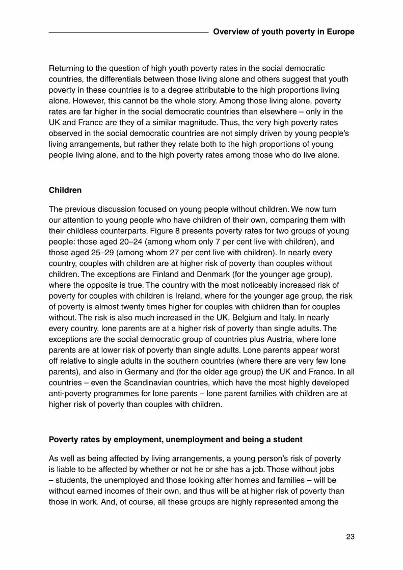
Children

The previous discussion focused on young people without children. We now turn our attention to young people who have children of their own, comparing them with their childless counterparts. Figure 8 presents poverty rates for two groups of young people: those aged 20–24 (among whom only 7 per cent live with children), and those aged 25–29 (among whom 27 per cent live with children). In nearly every country, couples with children are at higher risk of poverty than couples without children. The exceptions are Finland and Denmark (for the younger age group), where the opposite is true. The country with the most noticeably increased risk of poverty for couples with children is Ireland, where for the younger age group, the risk of poverty is almost twenty times higher for couples with children than for couples without. The risk is also much increased in the UK, Belgium and Italy. In nearly every country, lone parents are at a higher risk of poverty than single adults. The exceptions are the social democratic group of countries plus Austria, where lone parents are at lower risk of poverty than single adults. Lone parents appear worst off relative to single adults in the southern countries (where there are very few lone parents), and also in Germany and (for the older age group) the UK and France. In all countries – even the Scandinavian countries, which have the most highly developed anti-poverty programmes for lone parents – lone parent families with children are at higher risk of poverty than couples with children.

Poverty rates by employment, unemployment and being a student

As well as being affected by living arrangements, a young person’s risk of poverty is liable to be affected by whether or not he or she has a job. Those without jobs – students, the unemployed and those looking after homes and families – will be without earned incomes of their own, and thus will be at higher risk of poverty than those in work. And, of course, all these groups are highly represented among the

24


young: students mainly in the youngest age group, the unemployed mainly in the middle age group, and other economically inactive people, predominantly among women, in the oldest age group.

Figure 8 Poverty rates by presence of children

Social Democratic

0

40

60

80

20

Liberal Corporatist

%

Southern


Lone parentSingle person

Couple, no children Couple, with children

FIN DEN NETH UK IRE FRA GER AUS BEL POR SPA ITA GRE0

40

60

80

20

%

Aged 20–24

Aged 25–29

The analysis in Figure 9 divides young people into four categories: students, those with jobs, those who are formally unemployed and looking for work, and ‘other’. The ‘other’ group consists mainly of people who are looking after homes and families, but also includes those who are economically inactive because they are sick or disabled.

25


Figure 9 Poverty rates by activity status

0

40

60

20

%


WorkingStudent

Unemployed Other

Aged 16–19

0

40

60

20

%


Aged 20–24

0

40

60

20

%


Aged 25–29

Figure 9 shows that the risk of poverty varies greatly by activity status. Not unexpectedly, young people with jobs are, in general, the least likely to be poor. For the older two age groups, this is true for all countries, with the effect particularly marked in the oldest age group, for whom poverty levels among those in work are under 10 per cent in all countries, and well under 10 per cent in most. However, for the youngest age group, poverty levels for those in work are considerably higher. Only in Denmark are they under 10 per cent, and in Finland, Belgium, Spain and Greece they are over 20 per cent. In several countries, poverty rates are actually higher among those in work than among students. This partly refl ects the higher propensity of students to remain in the parental home compared with those with a job, but it also raises questions about the suffi ciency of young people’s wages.

26


It is worth devoting particular attention to the social democratic countries because, as we have previously remarked, they have particularly high rates of youth poverty, and as Figure 9 shows, they demonstrate a relatively different distribution of youth poverty from the other countries. In particular, the higher level of student poverty among the two older groups stands out in the social democratic countries. How far is this responsible for high overall rates of poverty in these countries? In Denmark, the rate of poverty among those in work, the unemployed and the economically inactive are generally lower (and in some cases much lower) than cross-country averages – and thus, the Danish peak in youth poverty rates may largely be attributed to the high level of poverty among students. In the Netherlands, poverty rates among those without jobs are higher than cross-country averages, but they are far from being the highest in the sample. In the Netherlands, therefore, student poverty is not solely responsible for high youth poverty rates, and some contribution is also made by relatively high poverty rates among other groups. In Finland, poverty rates are low among the ‘other’ group, but tend to be high among the unemployed and those with jobs. Since the numbers in the ‘other’ group are small relative to the other groups, it appears that the main driver behind youth poverty is student poverty, but that poverty among those with jobs and the unemployed also contributes.

Summary

We have measured the extent of youth poverty across 13 countries, by age group, by family structure and by employment status, and compared levels of youth poverty with levels of poverty among other age groups. We have shown that young people in many European countries are at higher-than-average risk of poverty and that, in some countries, young people are more likely than almost any other group to be poor. We have found signifi cant variations by country, and we have also identifi ed situations which put young people at particular risk of poverty.

Young people’s living arrangements and activity status vary widely between countries, with these variations being refl ected in the risk of poverty experienced by young people in each country. Living in one’s family of origin or living as a couple but without children tends to protect young people against poverty, whereas living alone or as a lone parent tends to increase the risk. Not having a job, whether one is a student, unemployed or out of the labour force, increases the risk of poverty, while having a job tends to protect young people against poverty.

Leaving aside those over 70, who in most countries suffer high rates of poverty, we fi nd that in Finland, Denmark and the Netherlands, young people are at a higher risk of poverty than any other age group, with youth poverty rates among the highest in

27


Europe. In the UK, young people are less susceptible to poverty than children are, but more susceptible than any other age group. In France, Germany, Austria and Belgium, poverty rates vary less with age, but in France particularly, young people suffer disproportionately from poverty. In Greece, Spain and Portugal, youth poverty rates are high in relation to most other countries, but not particularly high compared with other age groups in their own countries. In Italy, youth poverty rates are very high in comparison with other countries, and also in comparison with other age groups in Italy.

In almost all countries, the risk of poverty declines with age over the twenties, and is lower in the thirties than in the twenties. This is partly driven by changes in occupational status among young people (who are less likely to be studying or unemployed at later ages), but also by a reduced risk of poverty within groups: for example, those with a job are less likely to be poor in their late twenties than in their teens or early twenties. However, this is offset by the fact that more young people have left home at later ages, and more of them have had children.

Given that the existing literature on youth poverty is so scant, perhaps one of the main contributions of this section is to demonstrate that youth poverty is a major problem in many parts of Europe, and thus to identify this area of investigation as one wide open for further research.

The research in this chapter has been published as Aassve, A., Iacovou, M. and Mencarini, L. (2006) Youth Poverty and Transition to Adulthood in Europe. Demographic Research Vol. 15,pp. 21–50. It is available as open access on http://www.demographic-research.org/Volumes/Vol15/2/default.htm

28

5 How long do people stay poor? Poverty persistence and poverty recurrence

In the previous chapter, we established that young people face higher-than-average poverty rates in many European countries. Useful as this information is, it tells us no more than that a certain percentage of young people were poor at a particular point in time – crucially, it tells us nothing about the duration of poverty spells. And yet, this information on durations is vital. To reiterate a well-used example, a poverty rate of 10 per cent among 18–27-year-olds could mean that every single person in that country spends exactly one of the ten years between ages 18–27 in poverty, but is non-poor for the rest of the time – or it could mean that 10 per cent of young people are poor every single year between the ages of 18 and 27, while everyone else is non-poor the whole time. These two scenarios have very different implications for inequality and well-being in a society, and for measures to address poverty. Of course, the true story in every country will lie between the two extremes outlined, but the degree to which youth poverty is found to be persistent as opposed to transient will be extremely informative.

This information will be particularly useful in relation to the social democratic countries where, as we saw in Chapter 4, youth poverty rates are extremely high – both in relation to youth poverty rates in many other countries, but also (and particularly) in relation to the extremely low poverty rates experienced by the general population in these countries. If the high cross-sectional incidence of youth poverty in the social democratic countries merely shows that a large number of young people go through a short spell of poverty in the early adult years, this is likely to indicate less of a problem than a smaller number of people going through protracted spells of poverty.

In this chapter, we present statistics relating to the length of time young people spend in poverty; in Chapter 7, we present multivariate analysis of the factors associated with entry into and exit from poverty.

Poverty persistence

The fi rst measure we consider here is one of poverty persistence. The one-year poverty persistence rate measures the percentage of young people who, given that they were poor in one year, are also poor the next year. The two-year poverty

29

How long do people stay poor?…

persistence rate measures the percentage who, given they were poor in one year, have been continuously poor for the next two years, and so on.

Poverty persistence rates are shown in Figure 10(a)–(c). Each fi gure contains two sets of bars. The fi rst, thicker, bar, grey in colour, reproduces data from Table 1, and shows poverty rates for the age group in question. This fi rst series is measured against the left-hand axes. The other four narrow bars, superimposed upon the fi rst set, should be measured against the right-hand axes. These represent poverty persistence rates: the probability that a young person who is poor in one year remains poor every year for one year, two years, three years and four years, respectively.1 In each case, as we would expect, the probability of remaining poor declines with every extra year.

Figure 10 Poverty rates and poverty persistence for three age groups: (a) 16–19-year-olds; (b) 20–24-year-olds; (c) 25–29-year-olds

(a)

(b)

0

15

20

25

30

10

5


120

100

80

60

40

20

0

% still poor after 1 year (R/H axis) % still poor after 2 years (R/H axis)

% still poor after 3 years (R/H axis) % still poor after 4 years (R/H axis)

Poverty rates (L/H axis)

0

15

20

25

30

10

5


120

100

80

60

40

20

0

30


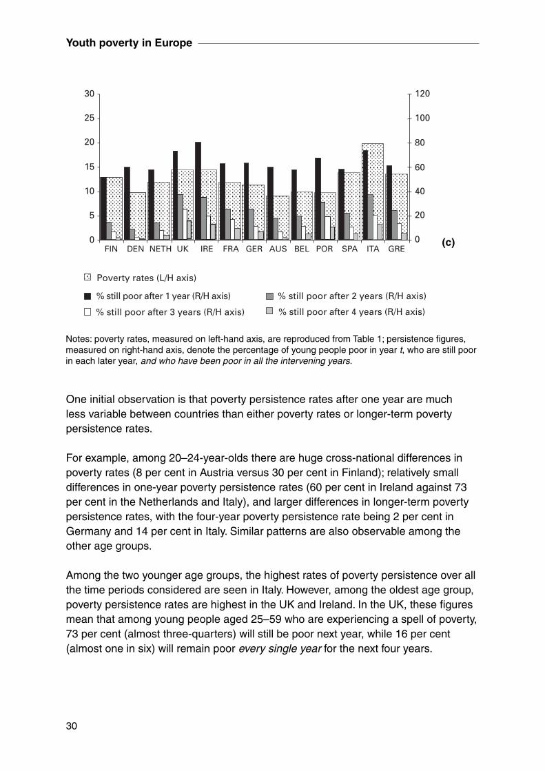
Notes: poverty rates, measured on left-hand axis, are reproduced from Table 1; persistence fi gures, measured on right-hand axis, denote the percentage of young people poor in year t, who are still poor in each later year, and who have been poor in all the intervening years.

(c)

One initial observation is that poverty persistence rates after one year are much less variable between countries than either poverty rates or longer-term poverty persistence rates.

For example, among 20–24-year-olds there are huge cross-national differences in poverty rates (8 per cent in Austria versus 30 per cent in Finland); relatively small differences in one-year poverty persistence rates (60 per cent in Ireland against 73 per cent in the Netherlands and Italy), and larger differences in longer-term poverty persistence rates, with the four-year poverty persistence rate being 2 per cent in Germany and 14 per cent in Italy. Similar patterns are also observable among the other age groups.

Among the two younger age groups, the highest rates of poverty persistence over all the time periods considered are seen in Italy. However, among the oldest age group, poverty persistence rates are highest in the UK and Ireland. In the UK, these fi gures mean that among young people aged 25–59 who are experiencing a spell of poverty, 73 per cent (almost three-quarters) will still be poor next year, while 16 per cent (almost one in six) will remain poor every single year for the next four years.

% still poor after 1 year (R/H axis) % still poor after 2 years (R/H axis)

% still poor after 3 years (R/H axis) % still poor after 4 years (R/H axis)

Poverty rates (L/H axis)

0

15

20

25

30

10

5


120

100

80

60

40

20

0

31


One question that we asked in Chapter 4 is whether the high rates of poverty in the social democratic countries among those in their early twenties could be thought of as somehow less serious because these poverty spells tend to be short-lived.

Figure 10 shows that this is at least partly true. Among the youngest age group, poverty persistence rates of two, three and four years are lower than the 13-country average in all three social democratic countries – and particularly in Denmark, where they are among the lowest in all the countries we study.

However, among 20–24-year-olds (the group at highest risk of poverty in the social democratic countries) persistence rates in the Netherlands are actually higher than in most other countries, and only fall to the 13-country average after four years. Persistence rates in Finland and Denmark are lower but, until we consider four-year rates, they are not noticeably lower than persistence rates in many other countries. Thus, although there is some justifi cation for the assertion that high youth poverty rates in Finland and Denmark are offset by the fact that poverty spells are unlikely to last for long, this is not the case for those aged 20–24 in the Netherlands, where 6 per cent of those who are poor in one year will still be poor four years later.

The poverty ‘hit rate’

The analysis above considered people who were continuously poor for various lengths of time. However, many individuals move in and out of poverty. The measure of poverty persistence outlined above treats a person who alternates each year between being poor and non-poor in exactly the same way as a person who was poor for one year and never poor again. However, the person who moves continuously in and out of poverty is arguably in a much worse situation than a person who is only poor once. Our second measure of poverty, which we call the ‘hit rate’, takes intermittent poverty into account.

The poverty ‘hit rate’ is calculated as the number of years a person is observed as being poor, divided by the total number of years in which the person is observed in the sample. This measure ranges between 0 (never poor) and 1 (poor in every single year). The classifi cations are defi ned as follows:

Classifi cation Percentage of years poor

Never poor noneOccasionally poor 1%–25%Moderately poor 26%–50%Frequently poor 51%–75%Constantly poor2 76%–100%

32


Figure 11 shows the proportions of young people in each of three age groups3 falling into each of these fi ve categories. Austria clearly does the best, with the highest proportion of young people in the ‘never poor’ category, and the lowest number in the ‘constantly poor’ category. And Italy arguably does worst, with a relatively small proportion in the ‘never poor’ category, and some of highest proportions in the ‘constantly’ and ‘frequently’ categories. However, Finland does very nearly as poorly, with very high levels of poverty persistence in the two older age groups and a very low proportion in the ‘never poor’ category.

Figure 11 Poverty ‘hit rates’: (a) 16–19-year-olds; (b) 20–24-year-olds; (c) 25–29-year-olds

(a)

(b)

0

40

60

20

%


80

100

Moderately poor

0

40

60

20

%


80

100

Occasionally poor

Never poor

Constantly poor

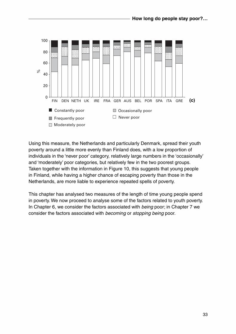
33


Using this measure, the Netherlands and particularly Denmark, spread their youth poverty around a little more evenly than Finland does, with a low proportion of individuals in the ‘never poor’ category, relatively large numbers in the ‘occasionally’ and ‘moderately’ poor categories, but relatively few in the two poorest groups. Taken together with the information in Figure 10, this suggests that young people in Finland, while having a higher chance of escaping poverty than those in the Netherlands, are more liable to experience repeated spells of poverty.

This chapter has analysed two measures of the length of time young people spend in poverty. We now proceed to analyse some of the factors related to youth poverty. In Chapter 6, we consider the factors associated with being poor; in Chapter 7 we consider the factors associated with becoming or stopping being poor.

(c)

Occasionally poor

Moderately poor

0

40

60

20

%


80

100

Frequently poor Never poor

Constantly poor

34

6 What factors are associated with being poor?

In Chapter 4, we examined the relationship between youth poverty and a range of factors: living away from the parental home; living alone; having children; and labour market activity status. All these factors were shown to be signifi cantly related to poverty, but this analysis should be understood as no more than suggestive, since it considers only one explanatory variable at a time, and does not control for any other background factors.

In this chapter, we perform multivariate analysis to examine how these other factors may also be affecting patterns of youth poverty. We do this using two different measures of poverty: the risk of income poverty and the index of deprivation, covering an inability to afford various items plus problems with the home and neighbourhood (described in Chapter 3). This multivariate analysis allows us to assess the relationships between poverty or deprivation and the different factors when all the effects are considered together.

In this analysis, we control for a wide range of personal characteristics: age (and age squared); sex; whether the person is employed; whether he or she has had the same job for two years or more; whether he or she is in education; whether the person has left the parental home; his or her marital status; and the number of children. Thus we are able to consider the effects of the various possible explanatory factors (such as living away from the parental home, having children and having a job) after taking account of differences in the personal characteristics of the young people who are in those situations.

The results of the analysis are shown in Figures 12(a) to 12(d), which focus on the most important factors. A brief description of the statistical methods used may be found in Appendix B. Table B1 provides descriptive statistics for all the explanatory variables used, Table B2 provides full results for the analysis of poverty, and Table B3 provides full results for the analysis of deprivation.

Results

Figure 12 shows the relative impact on poverty and deprivation of not being employed, not being in education, having left the parental home and being married, cohabiting and having children. The fi rst two graphs look at poverty, while the second two focus on deprivation.1

35


Figure 12 Results from regressions estimating poverty and deprivation: marginal effects: (a, b) poverty incidence; (c, d) deprivation index; (a, c) marginal effects of employment, education, parental home; (b, d) marginal effects of being married, cohabiting, number of children

FIN

Non employed Not in education Left parental home

0.2

0

–0.1

–0.2DEN NET UK IRE FRA GER AUS BEL POR SPA ITA GRE

0.1

0.3

(a)

Married Cohabiting Number of children

0.2

0

–0.1

–0.2

0.1

0.3

FIN DEN NET UK IRE FRA GER BEL POR SPA ITA GREAUS (b)

36


Non employed Not in education Left parental home

0.2

0

–0.1

–0.2

0.1

0.3

FIN DEN NET UK IRE FRA GER BEL POR SPA ITA GREAUS (c)

Married Cohabiting Number of children

0.2

0

–0.1

–0.2

0.1

0.3

FIN DEN NET UK IRE FRA GER BEL POR SPA ITA GREAUS (d)

It is clear that in all countries except for Ireland and the southern European countries, other risk factors are dwarfed by the risk of poverty and deprivation associated with having left the parental home. It is not surprising that living away from one’s parents increases one’s chance of being poor, since the parental income (which is likely to be higher than the young person’s income) is no longer available to the young person. However, the extremely large size of the effect of living away from the parental home is surprising – especially its size in relation to other factors, such as not being employed. An interesting feature of this fi nding is that the risk associated with living away from home is highest in the social democratic countries, closely followed by the UK and France – the very countries where home-leaving takes place earliest – whereas the impact of having left home in Ireland and the southern European countries (where home-leaving is much later) is considerably lower. This is the case in relation to both poverty and deprivation.

37


Note that these variations in risk are net of the effect of other factors. Because we have also controlled for marital and labour market status, the lower risk of poverty associated with living away from home that we observe in the southern European countries does not arise, because young southern Europeans are more likely to be married, or because they are less likely to leave home before having a job. However, we have not controlled for earnings, so it is possible that the lower risk of poverty in the south is associated with young people in these countries staying in the parental home until they have attained a level of earnings suffi cient to live on.

Turning to labour market activity, we fi nd (as we would expect) a relationship between non-employment and higher levels of poverty and deprivation. This relationship is fairly small in magnitude, but in most countries it is statistically signifi cant at the 5 per cent level, except in Denmark (poverty) and Greece (deprivation), where it is not signifi cant. The relationship is strongest in Italy, where those without a job have a risk of poverty 15 percentage points higher than those with a job – this effect is around twice the size of the effect of having left the parental home in Italy.

The effect of being in education varies across countries. Young people who have left education are less likely to be poor and/or deprived in Scandinavian countries, the UK and Germany. However, in Ireland, France, Austria and Belgium, there is no signifi cant association between having left education and one’s risk of poverty and deprivation. And in most Mediterranean countries, having left education confers no protection against poverty, and is actually associated with increased deprivation scores.

Figures 12(b) and (d) show the effects of marriage, cohabitation and childbearing. Both marriage and cohabitation appear to protect young individuals from poverty and deprivation, though marriage generally has a stronger effect than cohabitation (indeed, cohabitation does not appear to protect against deprivation in Portugal, Spain and Italy). This does not necessarily indicate that marriage is per se more protective than cohabitation, since different types of young people may choose to marry rather than to cohabit.

The effects of having children are smaller than the effects of marriage and cohabitation, and in the opposite direction: having children is associated with a generally higher risk of poverty and deprivation. The exceptions are, interestingly, Finland and Denmark, where children do not have any infl uence on the likelihood of poverty. This may be attributable to generous family support systems in these countries. The UK is notable here for being the most sensitive of all countries to family structure: in terms of poverty risk, there is a higher penalty in the UK than anywhere else for having children, and marriage and cohabitation protect more highly (in other words, there is a larger risk to being single).

38


Summary

In the social democratic group of countries, plus, to a lesser extent the UK and France, living away from the parental home is associated with a much higher risk of poverty, and much higher levels of non-monetary deprivation. These effects are far larger than the increased risks associated with non-employment, and also outweigh the protective effects of being married or living with a partner. The fact that these are countries where home-leaving typically occurs at a very early age may explain why it is associated with such high levels of poverty and deprivation; it also contributes to an understanding of why youth poverty levels are so high in these countries, particularly the social democratic countries. However, it raises a different question: Why, in countries where home-leaving is associated with such disadvantage, does it occur at such an early age? We return to this question in Chapter 8.

A second group of countries which may be identifi ed from this analysis is the southern European countries plus Ireland. This cluster is characterised by a low level of disadvantage associated with living away from home – in general, this disadvantage is of about the same magnitude, or somewhat less than, the disadvantage associated with not having a job, and is compensated for by the protective effects of marriage or cohabitation. In these countries, the level of disadvantage associated with having children, while smaller than that associated with many other factors, is larger than in other countries, with the exception of the UK, where young parents face the highest extra risk of poverty.

The social democratic countries, on the one hand, and the southern cluster, on the other, may be thought of as the two extremes; the other countries fall somewhere in the middle, with the UK and France closer to the social democratic pattern, while Austria and Belgium are closer to the southern pattern.

This chapter has looked at the factors associated with being poor. The next chapter looks at the factors associated with becoming poor, and stopping being poor.

Together with the research in Chapter 7, the research in this chapter has been published as Aassve, A., Davia, M,. Iacovou, M. and Mencarini, L. (2005) Poverty and the Transition to Adulthood: Risky Situations and Risky Events. ISER Working Paper 2005-23. It is downloadable from www.iser.essex.ac.uk/pubs/workpaps/pdf/2005-23.pdf

39

7 Entering and exiting poverty

The previous chapter examined the factors associated with being poor (or scoring highly on a deprivation index); we now turn to the questions of what makes a person become poor.

The fi rst part of this chapter examines transitions into poverty by those not currently poor, (‘who becomes poor?’) and the second considers transitions out of poverty by those who are currently poor (‘who stops being poor?’). Together with the results from Chapter 6, they help us build up a more complete picture of poverty trajectories and the factors which affect them.1

As in Chapter 6, the main results are presented graphically; full results are presented for the interested reader in Appendix C, Tables C1–C4.

Appendix C provides an overview of the statistical methods used for this chapter.

Controls

In Chapter 6, the following characteristics were taken into account through controls: age and age squared, sex, whether the person is employed, whether he or she has had the same job for two years or more, whether he or she is in education, whether the person has left the parental home, his or her marital status, and the number of children.

In this chapter, we use additional controls which indicate not only young people’s situation, but rather changes in their situation: leaving school, leaving home, getting married, and so on. In this way, we are able to estimate not only the effect of (for example) being married on the probability of escaping poverty, but also the additional effect of getting married.

This procedure generates two sets of results, which should be interpreted together. In the graphs below, two bars are shown for each variable, the fi rst depicting the effect2 of a young person being in that situation, and the second showing the effect of a recent change in that area. For example, Figure 13(a) shows that, in France, having left home is associated with an increase of 16 per cent in the risk of entering poverty. However, there is also a large effect, of 11 per cent, from just having left home. This should be added to the main effect to calculate the total effect on poverty of having left home in the past year: in this case, an increase in the risk of poverty of 27 per cent. Sometimes, the effects of being in a situation and the effect of recently entering

40


that situation work in opposite directions. For example, in Figure 13(c), the effect of marriage and cohabitation is generally to reduce the probability of poverty entry while, in many countries, the effect of having just entered a marriage or cohabitation is to raise the risk. In this case, the one should be subtracted from the other. For example, in the UK, cohabiting reduces a young person’s risk of poverty entry by 5 per cent. But being in the fi rst year of cohabitation increases the risk by 13 per cent. The net effect of these is that young people in their fi rst year of cohabitation face an increase in the risk of entering poverty of 8 per cent.

Entering poverty

Figure 13(a)–(c) display the main effects on entering poverty of leaving home, having children, employment, education, marriage and cohabitation. As was the case in the analysis discussed in previous chapters, the largest effect comes from young people living away from the parental home (Figure 13(a)). In all countries except for Ireland and the southern European countries, young people who have left home have a risk of entering poverty 10 percentage points higher than young people who still live at home – and in many countries, the increased risk is much higher (once again, Finland is off the scale, with an increase in risk of 37 percentage points. But there are additional sizeable effects on the risk of poverty entry from just having left home (i.e. from having left in the previous year) – in other words, young people who have left home in the past year are at a particularly high risk of becoming poor.

Figure 13 Marginal effects from regressions estimating poverty entry: (a) leaving parental home and having children; (b) non-employment and not being in education; (c) marriage and cohabitation.

(a)FIN

Left parental home Just left parental home

Has children

DEN NET UK IRE FRA GER AUS BEL POR SPA ITA GRE

New children last year

0.15

–0.1

0.1

0.2

–0.05

0

0.05

41


(b)

Non-employed Recently lost job

Not in education

0.15

–0.1

0.1

0.2

Just finished education

–0.05

0

0.05

FIN DEN NET UK IRE FRA GER AUS BEL POR SPA ITA GRE

(c)

Married Just married

Cohabiting

0.15

–0.1

0.1

0.2

Just started cohabiting

–0.05

0

0.05


42


The effects of having children are smaller, and we observe that it is newborn children (the ‘triggering event’), rather than the existence of older children, which is likely to push young families into poverty. Note that these effects, though positive in most countries, are signifi cant3 only in the Netherlands, the UK, Ireland, Austria, and all the southern European countries. Figure 13(b) deals with employment and being in education, and shows that young people without jobs are particularly susceptible to becoming poor in almost all countries. Non-employment is particularly serious for Italian youths, followed by Belgians, Irish, Germans, Spanish and Greeks. The only countries where this variable is not signifi cant are Denmark, Netherlands and Austria. Whereas non-employment is important in general, there is no additional effect of having experienced a recent job loss. In fact, in the Netherlands, Ireland and Italy, recent job loss reduces the risk of entering poverty by a small amount.

Figure 13(b) also shows the role of education. In those countries where students are more likely to be in poverty, they are also more likely to enter poverty: having fi nished one’s education is clearly related to a lower probability of becoming poor in Finland, Denmark, the Netherlands, the UK and Germany (and, to a lesser extent, Italy). However, there is no effect in any country of having left education in the last year.

Figure 13(c) shows the protective role of marriage and cohabitation against the risk of poverty entry. Marriage protects against entering poverty in all countries, and cohabitation nearly always, with Italy and Portugal being the only exceptions. We have already mentioned that cohabitation is still quite unusual in the Mediterranean countries, and may be particularly linked to unusual couples who may not be wealthy enough to afford the investment marriage requires. Only in France is there an additional positive effect of having married in the previous year. However, newly formed cohabitations are associated with a large and signifi cant increased risk of poverty in Finland, Denmark, the UK, France and Germany – these effects are larger than the protective effect of cohabitation in general, showing that young people in the fi rst year of cohabitation are at higher risk of poverty than those not living in a partnership. This interesting difference may indicate that young people tend to delay marriage until they are earning a certain amount, while cohabitations are formed despite the lack of economic resources, as a fi rst type of living arrangement after the leaving parental home.

Leaving poverty

The factors associated with leaving poverty are displayed in Figures 14(a)–(c). Consistent with previous fi ndings, leaving home (Figure 14(a)) reduces the chances of exiting poverty. In other words, among young individuals who are poor, living away

43


from the parental home reduces the chances of escaping poverty. And this effect is particularly relevant in the fi rst year after leaving the parental home: there is a large additional effect in most countries from having just left home, and indeed, in many countries this additional effect is the same size or bigger than the effect of living away from home. As before, the association between leaving home and being poor (here, exiting poverty) is less marked in Ireland and the southern European countries: again, the fact that youths in these countries tend to leave home to become married may explain this lower persistence in poverty among recent home-leavers there.

Parenthood also has a negative effect on a young person’s chances of exiting poverty – though, in all countries except for southern Europe, to a much smaller extent than living away from the parental home. Indeed, in most countries there is no signifi cant association between being a parent and the probability of exiting poverty: rather, it is the birth of a new baby which reduces the chances, and the effect of children tends to fade away with time. Newborn children tend to hinder escape from poverty in all countries except the Netherlands and Greece. This particular effect associated with newborn babies may be due to the fact that their mothers are likely to be taking time off work to look after them, and movements out of poverty are less likely at a time when the mother is not earning a full income.

Employment (Figure 14(b)) helps young people to escape poverty in all countries except Belgium and Denmark. Interestingly, there is no additional effect from having gained employment in the last year – on the contrary, having just found a job has a negative impact on exiting poverty. Moreover, in most countries this negative effect is of a similar order of magnitude to the positive effect of having employment, meaning that, overall in these countries, a young person who has just found a job has no higher chance of exiting poverty than a young person with no job at all. Put another way, the positive effect of employment is really restricted to those people who have held a job for at least a year. We were not able to discern, in this analysis, whether this is related to temporary jobs, but the political message is clear: it is not just employment, but stable and long-term employment, which is effective in lifting young people out of poverty.

44


Employed Recently employed

Not in education

0.2

–0.1

0.1

0.3

Just finished education

0

–0.2

–0.3FIN DEN NET UK IRE FRA GER AUS BEL POR SPA ITA GRE (b)

Figure 14 Marginal effects from regressions estimating poverty exit: (a) leaving parental home and having children; (b) employment and education; (c) marriage and cohabitation

(a)

Left parental home Just left parental home

Has children

–0.2

0.1

New children last year

–0.1

0

–0.3

–0.4

–0.5FIN DEN NET UK IRE FRA GER AUS BEL POR SPA ITA GRE

45


A relatively similar pattern emerges in relation to students: in almost all countries, those not in education are more likely to escape poverty (which is intuitively obvious, since the end of education implies in most cases a transition to employment, which naturally increases earnings, and therefore reduces poverty). But, in the majority of countries, just having left education has no signifi cant impact on escaping poverty – and in Denmark, the Netherlands, Germany and Belgium, leaving school in the last year has a negative effect on escaping poverty. This means that completion of education in these countries has a progressive effect on reducing poverty, which increases over time. Persistence in poverty diminishes in these countries with time out of education and in the labour market.

Figure 14(c) deals with living arrangements. As well as protecting young people from the risk of poverty as we saw in the previous chapter, both marriage and cohabitation make a positive contribution to the probability of leaving poverty. Marriage contributes signifi cantly to escaping poverty in Finland, the UK, Germany, Portugal and Spain; cohabitation contributes signifi cantly in all countries except Belgium and southern European countries,4 where cohabitation is quite unusual and related to lack of resources. In some cases (Finland, the UK, France and Belgium), the positive effect of marriage or cohabitation is not felt until more than a year into the relationship: this may be because there are costs inherent in starting out in marriage and cohabitation which are not immediately offset by the advantages.

Married Just married

Cohabiting

0.3

–0.2

0.2

0.4

Just started cohabiting

0.1

0

–0.1

FIN DEN NET UK IRE FRA GER AUS BEL POR SPA ITA GRE (c)

46


Summary

In this chapter, we have examined the factors associated with young people’s entry into and exit from poverty across Europe, in dynamic framework. Our results confi rm the results of the analysis in Chapter 6: living away from the parental home, non-employment and having children are associated with a higher risk of poverty entry, and a lower risk of poverty exit, whereas living with one’s parents and living with a partner are protective factors.

We fi nd that both living arrangements and education/labour market variables have an effect; however, living arrangements again have much the larger effect. In particular, not living with one’s parents is by far the most powerful predictor of moving into poverty. This result runs through all the analyses we performed. Marriage and cohabitation also protect against moving into poverty, while the presence of children has little effect, except in the year after they are born.

The effects of labour market factors are smaller, but still signifi cant. We fi nd that it is crucial to consider these factors in a dynamic context: in most countries, having a job does not improve a young person’s chances of exiting poverty until he or she has held the job for a year or more.

In fact, it is worth pointing out that, while this chapter has identifi ed a number of factors associated with a higher chance of escaping poverty, the only events which are likely to have a positive effect immediately are marriage and cohabitation – and even here, these immediate effects are not observable in all countries. Other routes towards fi nancial independence, such as fi nishing one’s education and getting a job, take time to manifest their effects. Thus, for young people who do go through a period of poverty, escaping from poverty may not be as simple a matter as (for example) leaving college and getting a job – rather, it may involve a much more protracted process.

Again, in this chapter, we have seen evidence of a continuum, with the Scandinavian countries, on the one hand, and the southern European countries plus Ireland, on the other, forming the two extremes; with the Netherlands, the UK and France falling in-between but closer to the Scandinavian end, while Germany, Belgium and Austria fall closer to the southern European end. In general, living away from one’s parents has the most negative effect towards the Scandinavian end, while having children and not having a job have the most negative effects towards the southern European end.

47


Returning to the start of the report, where we conceptualised youth as a series of transitions taking place in the spheres of the family and the labour market, this report confi rms what perhaps is intuitively obvious: many of these transitions come with very real risks. The labour market transitions of fi nishing one’s education and fi nding a job tend, in most countries, to improve young people’s economic situation. However, their effects for the age group we studied are not large; they often take time to manifest themselves; and, of course, the positive effect of fi nding a job is only present for young people who actually do fi nd a job. Meanwhile, the transitions young people make in the family sphere are likely to have a negative effect: leaving home is a time of great economic risk for many young people, particularly those in the Northern European countries; and becoming a parent also carries risks (though fortunately, these are relatively short-lived). Cohabitation and (particularly) marriage tend to shelter young people from the risk of poverty, but their protective effect is smaller than the negative effect of leaving home and, in any case, many young people wait for some time after leaving home before moving in with a partner.

In Chapter 8, we look in more detail at the effect of what is in most countries the most powerful predictor of youth poverty: leaving home.

Together with the research in Chapter 6, the research in this chapter has been published as Aassve, A., Davia, M,. Iacovou, M. and Mencarini, L. (2005) Poverty and the Transition to Adulthood: Risky Situations and Risky Events. ISER Working Paper 2005-23. It is downloadable from www.iser.essex.ac.uk/pubs/workpaps/pdf/2005-23.pdf.

48

8 Does leaving home make you poor?

Leaving home obviously matters. In all countries except Ireland and the southern European countries, not living in the parental home is by far the most powerful predictor for being poor and for entering poverty; it also yields large and signifi cant coeffi cients in equations estimating poverty exit. In the southern European countries, the estimated coeffi cients are smaller and of similar magnitude to some other factors, but they are still signifi cant.

Leaving home is worthy of further scrutiny, partly because the estimated relationships are so large, but also because some important questions remain unanswered. First, although previous analysis has established a strong relationship between home-leaving and youth poverty, it cannot identify whether this relationship is causal. That is, we have established that home-leaving is related to poverty, but we have not yet established whether home-leaving causes poverty. If there is a ‘selection effect’ – that is, if young people are more likely to leave home if they have certain characteristics which also make them more or less likely to be poor, then our previous estimates will not refl ect the impact of leaving home on poverty.

In our setting, it is not clear a priori which way the selection effect would go. On the one hand, it may be that young adults who would face a higher risk of poverty if they left home are more likely to stay at home for longer because they are aware of this higher risk. This would imply that the ‘true’, ‘causal’ effect of leaving home was actually higher than that suggested by the unadjusted relationship between home-leaving and poverty rates. On the other hand, it may be that certain characteristics are associated with both a higher propensity to leave the parental home, and a higher risk of poverty on leaving home. In this case, the raw fi gures would exaggerate the extra risk of poverty experienced by home-leavers, and the effect attributable to the home-leaving event would be lower.

The analysis in this chapter will also shed light on the puzzle referred to in Chapter 6: why, when home-leaving is so costly in terms of its associated poverty risk in the social democratic countries, are these precisely the countries where it occurs earliest? Economic theory would predict the opposite: that we would observe young people leaving home earlier in countries where it was relatively less costly to do so.

In this chapter, we analyse both poverty and two measures of deprivation, as described in Chapter 3. For clarity, however, in the explanation of our methods which follows, we refer to the outcome we are interested in as ‘poverty’, and return to deprivation later on in the chapter.

49


Understanding causality

To reiterate, the problem we are attempting to solve is as follows. We have established that there is a strong relationship between independent living and youth poverty. However, the extent to which leaving home ‘causes’ poverty is not clear. The causality could lie the other way round: it could be that young people who already have a greater propensity to be poor are more likely to leave home at a younger age. In this case, young people who choose to leave home would be somehow different from those who choose to remain living with their parents, and comparing poverty rates between the two groups would not be comparing like with like.

A standard approach to this problem is to use a technique known as Instrumental Variables. In our case, this would involve fi nding some variable correlated with leaving home, but not with the risk of poverty, or with certain other aspects of the relationship between poverty and leaving home. However, in this application it is diffi cult to think what such variables might be.

We want to estimate the effect of leaving home on poverty entry, net of other observed factors which infl uence the likelihood of entering poverty (such as whether one has a job, for example). Ideally, we would like to compare the risk of poverty for individuals leaving home, with the risk for the same individuals if they did not leave home (the ‘counterfactual’ situation). The problem is, of course, that for any given individual the two scenarios are mutually exclusive – a person cannot both leave home and not leave home.

Using Propensity Score Matching (PSM) techniques, we generate an approximation to the counterfactual situation, using data on individuals who have not left home, but who in all other respects are identical to individuals in our data set who have left home. Propensity Score Matching techniques are relatively complicated to implement, but the results are easy to interpret. The interested reader may consult Appendix D, which gives notes on the technique; otherwise, we move directly to discuss our results.

Results

Figure 15 relates to 20–24-year-olds1 who live with their parents in a non-poor household. The fi rst (light-coloured) bars show the extra risk of entering poverty associated with leaving home the following year, calculated as the difference between the percentage of ‘leavers’ entering poverty, and the number of ‘stayers’ entering poverty. This extra risk is largest in Finland (at 50 percentage points) and

50


lowest in Portugal (at around 3 percentage points). It is these numbers which may be subject to the problems outlined above, namely that they may not refl ect the causal effect of leaving home.

Figure 15 The extra risk of entering poverty associated with leaving home: descriptive and PSM estimates

PSM

0

0.1

Descriptive


0.2

0.3

0.4

0.5

0.6

The second (dark-coloured) bars in Figure 15 present PSM estimates. These are analogous to the fi rst set of fi gures, in that they represent the extra risk of poverty associated with the home-leaving event. However, the PSM results control for selection into leaving home (that is, for the fact that leavers and stayers may be different sorts of people), and thus may be thought of as the ‘causal’ effect of leaving home on poverty entry.

In many cases, the difference between the two sets of bars is small. However, these differences are statistically signifi cant in every country except for the Netherlands. The selection effect (represented by the difference in height between the two sets of bars) is not enormous in any country, but in several countries it is sizeable: descriptive analysis underestimates the ‘effect’ of leaving home on poverty entry by up to 5 percentage points in Finland, Denmark, France, Germany, Belgium and Portugal, while it overestimates the effect by a similar amount in Ireland and Austria.

It is worth making two points: fi rst, that the existence of signifi cant selection effects demonstrates the usefulness of PSM in this context, and second, that although selection effects are apparent, controlling for these effects does not change the pattern of our results. Leaving home is still associated with higher poverty entry rates in the Scandinavian countries than elsewhere: indeed, controlling for selection

51


slightly increases the estimated difference between the Scandinavian countries at one extreme, and Portugal and Spain at the other.

Overall, the estimates do not lend themselves to a clear clustering of countries consistent with modern welfare-regime theory such as that of Esping-Andersen (1990, 1999). While there is a clear ‘Scandinavian’ effect, with a high poverty entry risk on leaving home (55 per cent for Finland and 32 per cent for Denmark), there is a good deal of heterogeneity among three of the four other welfare-regime groups. The risk of entering poverty in the ‘Liberal’ cluster is relatively low; in the ‘conservative’ cluster (including the Netherlands), it is moderate – though a good deal higher in France and the Netherlands (26 per cent and 25 per cent) than in Belgium and Austria (14 per cent and 12 per cent). In the ‘southern’ cluster, Portugal and Spain show the lowest risks of all, at around 5 per cent, but in Italy it is 12 per cent, and in Greece it is over 20 per cent.

The analysis presented in Figures 16 and 17 is identical to that in Figure 15, except that Figures 16 and 17 deal not with poverty, but with monetary and non-monetary deprivation, respectively. The light-coloured bars show the extra increase in deprivation associated with home-leaving, not controlling for selection into leaving home, while the dark-coloured bars do control for selection, and thus show the extra risk in deprivation caused by leaving home.

Again, controlling for selection leaves the basic pattern of fi ndings unchanged, with the highest risks of deprivation associated with home-leaving being found in the Scandinavian countries plus France, and the lowest in the southern European countries.2 Thus, failing to correct for selection does not give an incorrect impression of the pattern of disadvantage. However, as far as monetary deprivation scores are concerned, failing to correct for selection does generally understate the extent of the disadvantage associated with leaving home. Everywhere except Ireland and Austria, the effect of leaving home, correcting for selection, is signifi cantly higher than the uncorrected effect, by 5 percentage points or more in several countries.

52


Figure 16 Increase in monetary deprivation scores associated with leaving home: descriptive and PSM estimates

Figure 17 Increase in non-monetary deprivation scores associated with leaving home: descriptive and PSM estimates

PSM

0

0.1

Descriptive

0.2

0.3

0.4

0.5

0.6


PSM

0

0.1

Descriptive

0.2

0.3

0.4

0.5

0.6

–0.1


Destination on leaving home

One possible explanation for the large inter-country differences in poverty entry rates on leaving home is that young people’s destinations on leaving home vary markedly between countries. The predominant pattern of home-leaving in the southern European countries is to move out of the parental home into a home shared with a husband or wife; by contrast, young Scandinavians are likely to spend a protracted period living alone. Poverty rates are generally higher for single-adult than for two-

53


adult households, so a proportion of inter-country differences in poverty entry rates may be due to these differences in housing destinations.

Figure 18 presents PSM estimates of poverty entry for all home-leavers (these are corrected for selection, and are the same fi gures as presented in the bars in Figure 15) and for the subsample of those who leave home to live as part of a childless couple (except for Denmark, where the very low numbers of young people exiting to form couples made this impossible).

Figure 18 PSM estimates by destination on leaving home

Those who leave home to form a couple

0

0.1

All leavers aged 20–24

0.2

0.3

0.4

0.5

0.6


In all countries, poverty entry rates are (as expected) lower for those who leave home to form a couple than for the group of leavers as a whole. However, it is clear that the differentials we observe cannot account for the entire differences in poverty entry rates between countries.

In Finland, the extra risk of poverty on leaving home as part of a couple is far higher than for any other country: even if all young people in Finland left home to form couples, they would still face a higher risk of poverty entry than young people in any other country. Similarly, even if all young people in the Netherlands and France left home as part of a couple, they would face a higher risk of poverty entry than young people in three out of the four southern European countries (and if all young Germans left home to form couples, they would face a higher risk of poverty than young people in Spain and Portugal). So, even after taking account of destinations on leaving home, there remain large differences in poverty outcomes between different groups of countries.

54


Summary

In this chapter, we have analysed the effect of leaving home on poverty entry and on changes in two deprivation indices, using a technique which estimates the causal effect of leaving home, net of pre-existing differences between young people who do and do not move out of their parents’ home.

In essence, we fi nd that the patterns observed in previous chapters (which do not control for selection) are fairly close approximations to the ‘causal’ effect of leaving home on poverty. However, the previous analysis does underestimate the causal effect slightly – particularly in those countries where the effect is large. We also fi nd these patterns to be replicated when deprivation rather than poverty forms the variable of interest: the results using monetary deprivation are close to those analysing poverty, while the effects on non-monetary deprivation are smaller.

One factor behind the observed cross-country differences in poverty risks associated with leaving home is that, in some countries, most young people move out of their parents’ home to live with a spouse or partner, while in other countries they are much more likely to live alone (which would tend to elevate the risk of poverty). However, we fi nd that, in countries where poverty risks on leaving home are high, they are also high for young people who leave as part of a couple – in other words, different destinations on leaving home can, at best, account for only a part of differences in poverty risks.

The analysis in this chapter has answered a number of questions successfully, but has left us with an interesting outstanding question. This is: why, in countries where leaving home is most costly (namely, the Scandinavian countries plus France and to a lesser extent the other Northern European countries), do young people leave home so early? We have already shown, in Chapter 5, that this cannot be explained away by differences between countries in the length of time that young people stay in poverty. Rather, future research should be directed at examining young people’s perceptions of risk within the labour market, and their perceptions of the role of the social security system in smoothing their incomes over the long-term.

The research in this chapter has been published as Aassve, A., Davia, M., Iacovou, M. and Mazzucco, M. (2005) Does Leaving Home Make You Poor? Evidence from 13 European Countries. ISER Working Paper 2005-24. It is downloadable from www.iser.essex.ac.uk/pubs/workpaps/pdf/2005-23.pdf

55

9 Conclusions

Young adulthood is a time of many life transitions and much uncertainty. In this report, we have shown that young adults are not the most vulnerable group in society, this position being held jointly by children and elderly people. However, young people in many countries, including the UK, face a risk of poverty considerably higher than that faced by most other age groups.

Several factors lie behind this elevated risk of poverty. First, because many young people still live with their parents and do not have jobs, some of the issues relating to child poverty are still pertinent, particularly for the 16–19 age group; this is evidenced by the fact that countries which have high levels of child poverty also tend to have high levels of poverty among the 16–19 group of young adults. Young adults in this age group, the majority of whom live with their parents, would be helped by social support systems aimed at compensating parents for the extra costs of bringing up children: both payments in respect of the young people themselves and payments in respect of younger siblings would help. Because the UK has one of the highest child poverty rates of the countries studied, and also one of the highest rates of poverty among 16–19-year-olds, such family support measures would be particularly relevant in this country.

For those who are somewhat older, we have found that many of the life changes involved in the transition to adulthood carry an inherent risk of poverty. The major risk, in all countries outside southern Europe, is leaving the parental home. Living away from the parental home is associated with an increased risk of poverty; with an increased risk of moving into poverty if one is not poor; and with a reduced risk of exiting poverty if one does happen to be poor. In addition, young people encounter an extra risk of poverty during the year in which they leave home.

In the UK, the poverty risk associated with leaving home is one of the highest observed in Europe: young people who have left home are 24 percentage points more likely to be poor than those of a similar age who still live at home. And if a young person is not poor in a particular year, he or she is 12 per cent more likely to become poor the following year if he or she does not live at home, and 18 per cent more likely to become poor if he or she is in the fi rst year of living away from home.

This suggests that, if some policy were being considered that would provide fi nancial assistance to young adults, this could usefully be targeted at those who are in the fi rst year or two of living away from the parental home. In reality, identifying this group may be harder than it appears, since many young adults are relatively fl uid

56


in their place of residence, and may move in and out of their parents’ home several times before the fi nal move to residential independence. However, the diffi culty of identifying the time when this transition actually takes place does not undermine our fi nding in this report that young people who have just left home are a group at particular risk of hardship, and in particular need of support.

Another respect in which the UK is different from other countries is in the particularly strong association for young adults in this country between having children and being poor. It is interesting to observe that in Austria and Germany, the increased risk associated with children is of the order of a couple of percentage points – and in Finland and Denmark, having children puts young adults at absolutely no added risk of poverty. In the Scandinavian countries, we attribute this to the twin policy instruments of comprehensive family support systems, which compensate families for the costs of children, and to family-friendly labour market systems, which mean that many mothers remain employed while they are bringing up young children. The UK stands in stark contrast to the Scandinavian countries, with each additional child increasing a young adult’s risk of poverty by 10 percentage points. There is certainly food for thought for policy makers here.

The cases of Germany and (particularly) Austria are noteworthy: in these two countries, poverty rates are exceptionally fl at across the life course, and young adults are at hardly any increased risk of poverty. Moreover, while factors such as leaving home and not having a job are risk factors in these countries, just as they are in other countries, the associated risks are much smaller. And when young people do become poor, poverty persistence rates are very low. The relatively advantaged position of young people in Austria and Germany may be attributable to a comprehensive system of vocational education, delivered via paid apprenticeships, which provides incomes and qualifi cations to sections of the young population which in other countries might be at risk of serious economic disadvantage.

Finally, this research has highlighted the importance of employment for young people. In fact, employment plays a smaller role in keeping young people out of poverty than do family factors, particularly living in the parental home. But it does play a part, and the important thing to note is that it plays its part cumulatively – the effect builds up over the years. It is not getting a job which forms a route out of poverty; rather, it is getting and keeping a job which is effective at raising young people out of poverty. At a time when several countries, including the UK, are implementing policies to encourage the employment of young people, it is as well to remember that this type of policy is likely to have little effect unless these jobs are created with a degree of longevity in mind.

57

Notes

Chapter 3

1 The United Nations General Assembly defi ned ‘youth’ as those persons falling between the ages of 15 and 24 years inclusive. This defi nition was made for International Youth Year, held around the world in 1985. All United Nations statistics on youth are based on this defi nition, as illustrated by the annual yearbooks of statistics published by the United Nations system on demography, education, employment and health.

2 The full range of ECHP data is available only for individuals aged 17 and over, though data on household structure is available for 16-year-olds.

3 The reader should note that this procedure was not possible using Finnish data, and thus for Finland, all data relates to incomes for year t – 1.

4 General references for the development of these measures are contained in Lemmi and Betti (2006), Cerioli and Zani (1990) and Cheli and Lemmi (1995).

5 Approaches of this kind applied to poverty analysis of European countries are becoming quite common (Eurostat (2002), Aassve et al. (2005b)). For a fully detailed explanation of how these indices are estimated, see Aassve et al. (2007)

Chapter 4

1 In the equivalence scale that we use to calculate poverty rates (see Chapter 3) teenagers of 14 and over are considered to need more income to support them than children. The peak in poverty rates towards the mid-teens may at least partly be a refl ection of these higher assumed needs.

Chapter 5

1 These fi gures are based on young people who were poor at some year t, and who were re-interviewed each year until the relevant date. The sample has been re-weighted to control for attrition, but no correction has been made for the fact that low incomes and/or poverty may be positively associated with attrition.

58


2 Strictly, this should read ‘more or less constantly poor’.

3 Here, age is measured as the person’s age in the fi rst time period in which they were observed. Thus, many individuals will in reality have crossed from one age bracket to the next during the period of observation.

Chapter 6

1 This measure of non-monetary deprivation is discussed in Chapter 3. It is calculated from a range of variables refl ecting economic well-being, including the inability to afford basic requirements; inability to afford a range of consumer durables, the lack of certain domestic facilities, other problems with one’s home, and problems with the neighbourhood in which one lives.

Chapter 7

1 For several reasons, this type of analysis is more diffi cult using continuous deprivation indices. Results examining changes in deprivation scores across time are available from the authors upon request.

2 Strictly, the analytical techniques in this chapter estimate relationships between the explanatory variables and the probability of entering or exiting poverty, rather than effects – which would carry some implication of causality. However, we are able to explain how to interpret the coeffi cients much more succinctly by calling the coeffi cients ‘effects’, so we have done this.

3 By which we mean: statistically signifi cant at the 5 per cent level or better

4 The odd positive effect of recent cohabitation on leaving poverty in Portugal is probably related to the small sample size in that particular cell.

Chapter 8

1 Full results for all age groups, plus bootstrapped standard errors, are shown in Appendix D, Table D1. In general, the effect of leaving home on poverty entry is lower for older age groups, which is not surprising, given that older youths tend to have higher income and more stable employment.

59

Notes

2 The average deprivation score of young people living at home is 0.16 with a standard deviation of 0.27; in this context, the increases in deprivation associated with leaving home are relatively large.

Appendix B

1 An alternative is to use fi xed effects models. We have repeated all our analysis using fi xed effects models, and fi nd that the results of the random and fi xed effects models are very similar.

Appendix D

1 Under this procedure, it is possible to pair individuals in the treatment group with any number of individuals in the control group. The number three was selected in order to give the best trade-off between bias and variance. Those with only one or two near neighbours were included; those with no near neighbours were excluded.

2 Table D2 also contains a number of indicators of the quality of the matching process, namely, the reduction in bias due to matching and the number of cases lost due to trimming and conditioning on the common support.

60

References

Aassve, A., Billari. F.C., Mazzuco, S. and Ongaro, F. (2003) ‘Leaving home: a comparative analysis of ECHP data’, Journal of European Social Policy, Vol. 12, No. 4, pp. 259–75.

Aassve, A., Iacovou, M. and Mencarini, L (2005a) Youth Poverty in Europe: What Do We Know? Working Paper of Institute for Social and Economic Research, Paper 2005-02. Colchester: University of Essex

Aassve, A., Mazzucco, S. and Mencarini, L. (2005b) ‘Childbearing and wellbeing: a comparative analysis of the European welfare regimes’, Journal of European Social Policy, Vol. 5, No. 4, pp. 283–99

Aassve, A., Davia, M., Iacovou, M. and Mencarini, L. (2005c) Poverty and the Transition to Adulthood: Risky Situations and Risky Events. Working Paper of Institute for Social and Economic Research, Paper 2005-23 (PDF) Colchester: University of Essex.

Aassve, A., Iacovou, M. and Mencarini, L. (2006) ‘Youth poverty and transition to adulthood in Europe’, Demographic Research, Vol. 15, pp. 21–50. Available at http://www.demographic-research.org/Volumes/Vol15/2/

Aassve, A., Betti, G. Mazzuco, S. and Mencarini, L. (2007) ‘Marital disruption and economic well-being: a comparative analysis’, Journal of the Royal Statistical Society A, Vol 170, pp. 781–99

Becker, S. and Ichino, A. (2002) ‘Estimation of average treatment effects based on propensity scores’, STATA Journal, Vol. 2, No. 4, pp. 358–77

Boys, A., Marsden, J. and Strang, J. (2001) ‘Understanding reasons for drug use amongst young people: a functional perspective’, Health Education Research, Vol. 16, No. 4, pp. 457–69

Bradbury, B. and Jäntti, M. (1999) Child Poverty Across Industrialized Nations. Innocenti Occasional Papers Economic and Social Policy Series No. 71, September. Florence: UNICEF

Bradley, H. and van Hoof, J. (2005) Young People in Europe: Labour Markets and Citizenship. Bristol: The Policy Press

61

References

Brewer, M., Goodman, A., Shaw, J. and Shephard, A. (2005) Living Standards, Inequality and Poverty: 2005 Election Briefi ng Note No. 9. London: Institute for Fiscal Studies

Caliendo, M. and Kopeinig, S. (2005) Some Practical Guidance for the Implementation of Propensity Score Matching. IZA Working Paper No. 1588. Available at http://repec.iza.org/dp1588.pdf

Cantillon, B. and Van den Bosch, K. (2003) Social Policy Strategies to Combat Income Poverty of Children and Families in Europe. Maxwell School of Citizenship and Public Affairs Working Paper No. 336. New York: Syracuse University

Cantó-Sanchéz, O. and Mercader-Prats, M. (1999) Poverty among Children and Youth in Spain: The Role of Parents and Youth Employment Status. Document de Treball 99.07. Barcelona: Departament d’Économia Aplicada, Universitat Autònoma de Barcelona

Catan, L. (2004) Becoming Adult: Changing Youth Transitions in the 21st Century. Brighton: Trust for the Study of Adolescence

Cerioli, A. and Zani, S. (1990) ‘A fuzzy approach to the measurement of poverty’, in C. Dagum and M. Zenga (eds) Income and Wealth Distribution, Inequality and Poverty, Studies in Contemporary Economics. Berlin: Springer

Cheli, B. and Lemmi, A. (1995) ‘A totally fuzzy and relative approach to the multidimensional analysis of poverty’, Economic Notes, Vol. 24, pp. 115–34

Corijn, M. and Klijzing, E. (2001) Transitions to Adulthood in Europe. Dordrecht: Kluwer:

Esping-Andersen, G. (1990) Three Worlds of Welfare Capitalism. Cambridge: Polity Press

Esping-Andersen, G. (1999) Social Foundations of Post Industrial Economies. Oxford: Oxford University Press

European Commission (2001) European Commission White Paper: A New Impetus for European Youth. Brussels: Commission of the European Communities

Eurostat (2002) Income, Poverty and Social Exclusion: Second Report. Luxembourg: European Social Statistics

62


Fahmy, E. (2002) Youth, Poverty and Social Exclusion. Working Paper 27. Bristol: Townsend Centre for International Poverty Research, University of Bristol

Ferrera, M. (1996) ‘The “southern model” of welfare in social Europe’, Journal of European Social Policy, Vol. 6, No. 1, pp. 17–37

Greene, W.H. (2003) Econometric Analysis, 5th edition. New Jersey: Prentice Hall-Pearson

Hammer, T. (2003) Youth Unemployment and Social Exclusion in Europe. Bristol: The Policy Press

Hansen, K. (2003) ‘Education and the crime–age profi le’, British Journal of Criminology, Vol. 43, pp. 141–68

Heuberger, R. (2003) ‘What household gets what income?’ Paper presented at the EPUNET Conference, Essex, UK

Iacovou, M. (2002) ‘Regional differences in the transition to adulthood’, Annals of the American Association of Political and Social Science, No. 580, pp. 40–69

Iacovou, M. and Berthoud, R. (2001) Young People’s Lives: A Map of Europe. Colchester: University of Essex, Institute for Social and Economic Research. Available atwww.iser.essex.ac.uk/pubs/iserreps/pdf/002.pdf

Jones, G. (2002) The Youth Divide: Diverging Paths to Adulthood. York: York Publishing Services/Joseph Rowntree Foundation

Kangas, O. and Palme, J. (2000) ‘Does social policy matter? Poverty cycles in the OECD countries’, International Journal of Health Services, Vol. 30, pp. 335–52

Lemmi, A. and Betti, G. (2006) Fuzzy Set Approach to Multidimensional Poverty Measurement. New York: Springer

Micklewright, J. (2004) Child Poverty in English-Speaking Countries. LIS Working Paper No. 376. New York: Syracuse University

Müller, W., Steinmann, S. and Ell, R. (1998) ‘Education and labor market entry in Germany’, in S. Yossi and W. Müller (eds) From School to Work. A Comparative Study of Educational Qualifi cations and Occupational Destinations. Oxford: Clarendon Press

63

References

Nicoletti, C. and Peracchi, F. (2005) ‘Survey response and survey characteristics: micro-level evidence from the European Community Household Panel’, Journal of the Royal Statistical Society Series A (Statistics in Society), Vol. 168, No. 4, pp. 763–81

Offi ce for National Statistics (2004) Social Trends. London: HMSO

Peracchi, F. (2002) ‘The European Community Household Panel: a review’, Empirical Economics, Vol. 27, pp. 63–90

Rosenbaum, P.T. and Rubin, D.B. (1983) ‘Constructing a control group using multivariate matching sampling methods that incorporate the propensity score’, The American Statistician, Vol. 39, No. 1, 33–8

Rugg, J. (1999) Young People, Housing and Social Policy. London: Routledge

Russell, H. and O’Connell, P.J. (2001) ‘Getting a job in Europe: the transition from unemployment to work among young people in nine European countries’, Work, Employment and Society, Vol. 15, No. 1, pp. 1–24

Shucksmith, J. and Spratt, J. (2002) Young People’s Self Identifi ed Health Needs. HEBS Young People and Health Initiative Working Paper, University of Aberdeen

Sianesi, B. (2004) ‘An evaluation of the Swedish system of active labour market programmes in the 1990s’, Review of Economics and Statistics, Vol. 86, No. 1, pp. 133–55

Smeeding, T. and Ross Phillips, K. (2002) ‘Cross-national differences in employment and economic suffi ciency’, Annals of the American Association of Political and Social Science, No. 580, pp. 103–33

Smith, J.A. and Todd, P. (2005) Does matching overcome Lalonde’s critique of nonexperimental estimators?’, Journal of Econometrics, Vol. 125, No. 1–2, pp. 305–53

Verma, V. and Betti G. (2005) ‘Sampling errors for measures of inequality and poverty’, Invited paper in Classifi cation and Data Analysis, CLADAG, Parma, 6–8 June

Wooldridge, J.M. (2004) Econometric Analysis of Cross Section and Panel Data. Cambridge, MA: MIT Press

64


Wooldridge, J.M. (2005) ‘Simple solutions to the initial conditions problem in dynamic, nonlinear panel data models with unobserved heterogeneity’, Journal of Applied Econometrics, Vol. 20, No. 1, pp. 39–54

65

Appendix A Variables used for calculating deprivation index1 Basic non-monetary deprivation – these concern inability to afford basic

requirements:keeping the home (household’s principal accommodation) adequately warmpaying for a week’s annual holiday away from homereplacing any worn-out furniturebuying new, rather than second-hand clotheseating meat chicken or fi sh every second day, if the household wanted tohaving friends or family for a drink or meal at least once a monthinability to meet payment of scheduled mortgage payments, utility bills or hire

purchase instalments.

2 Secondary non-monetary deprivation – an item refl ect deprivation only if the household could not afford ita car or vana colour tva video recordera microwavea dishwashera telephone

3 Lacking housing facilities – these concern the absence of basic housing facilities:a bath or showeran indoor fl ushing toilethot running water

4 Housing deterioration – these concern serious problems with accommodation:leaky roofdamp walls, fl oors, foundation etc.rot in window frames or fl oors

5 Environmental problems – these concern problems with the neighbourhood and the environment:shortage of spacenoise from neighbours or outsidedwelling too dark/not enough lightpollution, grime or other environmental problems caused by traffi c or industryvandalism or crime in the area

66

Appendix B Statistical methods used in Chapter 6

The longitudinal nature of the ECHP implies that households and individuals who are part of the survey are observed repeatedly over time. Thus, observations from one year to another are clearly not independent, and conventional statistical methods as used for cross-sectional data are not suitable. Here, we use random effects regression models, which are designed to control for repeated observations on the same individuals.

We do not describe the methods in detail here; descriptions may be found in advanced econometric textbooks (Greene, 2003; Wooldridge, 2004).

When using poverty status (which is a dichotomous variable) as the dependent variable, we estimate random effects probit models; when we consider the deprivation index (which is a continuous measure), we estimate linear random effects models.1 All estimates are reported in terms of their marginal effects, and thus may be interpreted in the essentially the same way as ordinary least squares coeffi cients.

67

Appendix B

Tab

le B

1 D

escr

ipti

ve s

tati

stic

s

FIN

D

K

NE

T

UK

IR

E

FR

G

ER

A

T

BE

L

PT

E

S

ITA

G

R

Poo

r 0.

174

0.16

4 0.

136

0.20

0 0.

137

0.23

7 0.

190

0.19

0 0.

154

0.10

4 0.

218

0.13

4 0.

222

Dep

rivat

ion

0.19

5 0.

149

0.16

9 0.

189

0.15

0 0.

207

0.22

9 0.

184

0.18

7 0.

127

0.14

4 0.

126

0.20

7E

ntry

into

pov

erty

0.

074

0.05

5 0.

045

0.06

5 0.

043

0.07

0 0.

072

0.06

7 0.

048

0.03

6 0.

095

0.05

1 0.

063

Exi

t fro

m p

over

ty

0.26

7 0.

258

0.26

1 0.

252

0.27

1 0.

226

0.27

8 0.

278

0.26

3 0.

273

0.23

6 0.

261

0.24

6A

ge

23.4

32

23.2

08

23.0

55

23.1

90

22.3

41

23.2

96

22.9

34

22.8

54

22.7

74

22.3

92

22.3

25

23.4

22

23.2

39P

ost-

com

puls

ory

edu

catio

n (y

r)

3.10

8 0.

976

1.47

4 2.

336

1.92

3 2.

697

2.73

0 2.

191

1.96

0 2.

520

2.89

3 1.

170

2.14

2F

emal

e 0.

516

0.53

5 0.

526

0.50

5 0.

485

0.49

6 0.

509

0.49

1 0.

479

0.48

2 0.

499

0.51

4 0.

523

Em

ploy

ed

0.88

7 0.

900

0.88

0 0.

775

0.83

3 0.

697

0.62

8 0.

740

0.82

9 0.

893

0.83

4 0.

825

0.78

4N

on-e

mpl

oyed

0.

113

0.10

0 0.

120

0.22

5 0.

167

0.30

3 0.

372

0.26

0 0.

171

0.10

7 0.

166

0.17

5 0.

216

Rec

ently

non

-em

ploy

ed

0.08

1 0.

035

0.04

0 0.

015

0.04

0 0.

029

0.03

0 0.

044

0.02

3 0.

017

0.16

0 0.

062

0.04

1R

ecen

tly e

mpl

oyed

0.

193

0.10

7 0.

069

0.11

9 0.

197

0.07

5 0.

119

0.14

7 0.

130

0.14

5 0.

137

0.05

9 0.

214

Em

ploy

ed ≥

2 yr

0.

225

0.30

0 0.

251

0.22

3 0.

251

0.18

7 0.

193

0.15

4 0.

332

0.37

0 0.

161

0.26

6 0.

201

Not

in e

duca

tion

0.68

4 0.

651

0.57

3 0.

673

0.72

1 0.

660

0.73

4 0.

649

0.73

6 0.

750

0.56

4 0.

663

0.87

8Ju

st le

ft ed

ucat

ion

0.03

1 0.

004

0.00

9 0.

016

0.03

3 0.

017

0.02

6 0.

022

0.01

2 0.

035

0.04

9 0.

015

0.02

2Le

ft pa

rent

al h

ome

0.70

2 0.

553

0.39

2 0.

483

0.20

7 0.

183

0.26

3 0.

207

0.26

1 0.

307

0.55

3 0.

489

0.60

0Ju

st le

ft pa

rent

al h

ome

0.00

9 0.

009

0.00

9 0.

009

0.00

8 0.

006

0.00

6 0.

006

0.00

6 0.

006

0.01

6 0.

007

0.01

1M

arrie

d 0.

121

0.17

7 0.

207

0.16

3 0.

106

0.15

3 0.

216

0.17

2 0.

265

0.15

4 0.

136

0.23

6 0.

195

Just

mar

ried

0.02

0 0.

017

0.01

3 0.

031

0.01

7 0.

022

0.03

2 0.

034

0.04

3 0.

026

0.02

2 0.

006

0.02

5C

ohab

iting

0.

350

0.21

5 0.

133

0.20

1 0.

032

0.01

1 0.

009

0.02

2 0.

017

0.09

0 0.

239

0.14

1 0.

214

Just

sta

rtin

g co

habi

tatio

n 0.

059

0.03

2 0.

025

0.03

7 0.

008

0.00

3 0.

003

0.00

6 0.

005

0.02

3 0.

056

0.02

7 0.

049

No

long

er m

arrie

d, s

ingl

e 0.

008

0.00

4 0.

007

0.00

5 0.

002

0.00

2 0.

007

0.00

5 0.

009

0.00

9 0.

006

0.01

4 0.

014

Chi

ldre

n <

1 yr

old

0.

043

0.01

8 0.

032

0.05

2 0.

026

0.02

1 0.

038

0.02

4 0.

040

0.04

2 0.

035

0.01

2 0.

050

Chi

ldre

n ≥

1 yr

old

0.

333

0.21

4 0.

285

0.31

2 0.

215

0.16

3 0.

290

0.17

3 0.

361

0.31

5 0.

323

0.38

3 0.

409

n 5,

775

4,85

3 8,

632

8,72

0 9,

302

13,6

98

14,1

52

6,68

2 5,

558

15,4

71

20,4

62

21,2

88

12,9

30

Sou

rce:

EC

HP,

Wav

es 1

–8.

68


Tab

le B

2 R

and

om

eff

ects

pro

bit

reg

ress

ion

; dep

end

ent

vari

able

is p

over

ty s

tatu

s b

ased

on

60%

of

med

ian

net

eq

uiv

alis

ed h

ou

seh

old

inco

me

F

IN

DK

N

ET

U

K

IRE

F

R

GE

R

AT

B

EL

P

T

ES

IT

A

GR

Age

–0

.004

0.

000

0.03

5***

0.

008

–0.0

33**

* 0.

042*

**

0.00

8 –0

.011

**

0.00

2 –0

.022

***

–0.0

1 0.

002

0.01

1

(–0.

253)

(–

0.03

8)

–5.2

37

(0.7

39)

(–6.

509)

(5

.168

) (1

.954

) (–

3.25

8)

(0.3

16)

(–4.

556)

(–

1.76

8)

(0.2

74)

(1.4

16)

Age

squ

ared

–0

.001

0.

000

–0.0

01**

* –0

.001

**

0.00

1***

–0

.001

***

–0.0

00**

* 0.

000*

0.

000

0.00

0***

0.

000

0.00

0 –0

.000

*

(–1.

811)

(–

1.44

9)

(–6.

911)

(–

3.22

0)

(5.2

11)

(–6.

945)

(–

3.46

4)

(2.1

99)

(–1.

249)

(3

.671

) (0

.234

) (–

0.56

9)

(–2.

123)

Year

s in

edu

catio

n 0.

001

0.00

5***

0.

000

0.00

2 –0

.002

**

–0.0

03**

* 0.

003*

**

0.00

0 –0

.001

–0

.005

***

–0.0

05**

* –0

.010

***

–0.0

10**

*

(0.5

52)

(4.0

32)

(–0.

128)

(1

.708

) (–

2.64

2)

(–3.

448)

(3

.539

) (–

0.00

3)

(–1.

155)

(–

7.11

6)

(–6.

472)

(–

9.90

3)

(–8.

413)

Fem

ale

–0.0

34**

* –0

.011

–0

.006

–0

.028

***

–0.0

02

–0.0

18**

* –0

.008

**

0.00

2 –0

.004

–0

.011

**

–0.0

03

–0.0

06

–0.0

12*

(–

4.49

1)

(–1.

717)

(–

1.31

4)

(–3.

905)

(–

0.64

6)

(–3.

318)

(–

2.77

7)

(0.7

54)

(–0.

769)

(–

2.84

8)

(–0.

676)

(–

0.95

7)

(–1.

986)

Not

em

ploy

ed

0.05

2***

0.

000

0.02

2**

0.06

2***

0.

044*

**

0.03

3***

0.

049*

**

0.01

5**

0.07

5***

0.

044*

**

0.05

7***

0.

144*

**

0.05

6***

(4

.038

) (–

0.03

7)

(2.6

69)

(6.5

39)

(6.5

33)

(5.0

88)

(8.2

27)

(2.8

67)

(5.2

02)

(7.3

76)

(9.8

39)

(15.

471)

(8

.254

)

In s

ame

job

>2

yr

–0.0

80**

* –0

.062

***

–0.0

59**

* –0

.060

***

–0.0

38**

* –0

.088

***

–0.0

32**

* –0

.022

***

–0.0

42**

* –0

.036

***

–0.0

66**

* –0

.088

***

–0.0

50**

*

(–12

.697

) (–

10.5

66) (

–13.

082)

(–9

.472

) (–

11.8

96)

(–19

.357

) (–

12.8

87)

(–7.

455)

(–

9.24

7)

(–10

.822

) (–

17.9

52) (

–18.

265)

(–9

.719

)

Not

in e

duca

tion

–0.0

42**

* –0

.054

***

–0.0

33**

* –0

.109

***

–0.0

08*

–0.0

18**

–0

.046

***

–0.0

10**

–0

.007

0.

005

0.00

1 –0

.031

***

–0.0

02

(–4.

873)

(–

6.17

3)

(–5.

830)

(–

7.29

8)

(–2.

246)

(–

2.72

1)

(–9.

337)

(–

2.67

6)

(–1.

160)

(1

.141

) (0

.198

) (–

4.16

1)

(–0.

239)

Left

pare

ntal

hom

e 0.

537*

**

0.23

2***

0.

240*

**

0.23

9***

0.

066*

**

0.27

2***

0.

178*

**

0.15

9***

0.

145*

**

0.01

3 0.

084*

**

0.07

6***

0.

079*

**

(29.

209)

(1

8.49

2)

(17.

929)

(2

4.10

4)

(6.0

78)

(22.

364)

(1

7.92

8)

(9.0

30)

(7.4

29)

(1.8

18)

(6.0

74)

(4.4

36)

(6.1

51)

Mar

ried

–0.0

88**

* –0

.060

***

–0.0

76**

* –0

.111

***

–0.0

30**

* –0

.093

***

–0.0

53**

* –0

.030

***

–0.0

48**

* –0

.038

***

–0.0

71**

* –0

.087

***

–0.0

80**

*

(–13

.720

) (–

10.7

46) (

–15.

857)

(–1

6.88

9) (

–8.3

83)

(–19

.471

) (–

15.9

13)

(–10

.431

) (–

8.91

2)

(–7.

448)

(–

12.9

54) (

–12.

073)

(–1

1.07

9)

Coh

abiti

ng

–0.0

99**

* –0

.099

***

–0.0

65**

* –0

.081

***

–0.0

26**

* –0

.071

***

–0.0

36**

* –0

.024

***

–0.0

35**

* –0

.023

***

–0.0

52**

* –0

.070

***

–0.0

61**

*

(–14

.382

) (–

13.3

90) (

–15.

117)

(–1

4.00

3) (

–8.2

63)

(–15

.856

) (–

15.4

77)

(–10

.585

) (–

8.37

9)

(–3.

645)

(–

9.09

9)

(–8.

029)

(–

7.46

4)

No

long

er m

arrie

d, s

ingl

e –0

.032

–0

.017

0.

003

0.06

9 0.

113

0.03

6 0.

039*

–0

.004

–0

.011

–0

.003

0.

014

0.08

0.

056

(–

1.49

9)

(–0.

749)

(0

.113

) (1

.942

) (1

.241

) (0

.980

) (2

.309

) (–

0.45

3)

(–0.

739)

(–

0.23

1)

(0.5

30)

(1.0

53)

(1.3

67)

No.

of c

hild

ren

0.00

7 –0

.013

0.

059*

**

0.09

7***

0.

036*

**

0.04

3***

0.

023*

**

0.01

4***

0.

029*

**

0.05

0***

0.

074*

**

0.06

2***

0.

055*

**

(0.9

02)

(–1.

888)

(1

1.62

0)

(16.

251)

(9

.913

) (8

.727

) (9

.463

) (4

.856

) (6

.307

) (1

2.46

8)

(13.

766)

(8

.751

) (8

.857

)

No.

of o

bser

vatio

ns

9,86

1 7,

996

13,8

23

14,7

79

15,1

60

21,5

19

21,3

96

10,8

18

8,61

4 22

,467

30

,741

31

,397

19

,246

Sou

rce:

EC

HP,

Wav

es 1

–8.

Ref

eren

ce g

roup

: Men

em

ploy

ed <

2 yr

, stil

l in

educ

atio

n, in

par

enta

l hom

e, s

ingl

e an

d ne

ver

mar

ried.

*0.1

; **0

.05;

***

0.00

1.

69

Appendix B

Tab

le B

3 R

and

om

eff

ects

lin

ear

reg

ress

ion

of

tota

l dep

riva

tio

n in

dex

F

IN

DK

N

ET

U

K

IRE

F

R

GE

R

AT

B

EL

P

T

ES

IT

A

GR

Age

0.

009

0.03

1*

0.06

2***

0.0

19*

–0.0

08

0.02

4***

0.0

30**

* 0.

007

–0.0

05

–0.0

03

0.00

4 0.

009

0.01

(0

.913

) (2

.489

) (8

.629

) (2

.263

) (–

1.17

2)

(3.6

72)

(4.7

88)

(1.1

21)

(–0.

583)

(–

0.48

8)

(0.7

38)

(1.7

46)

(1.3

21)

Age

squ

ared

0.

000

–0.0

01**

–0

.002

***

–0.0

01**

0.

000

–0.0

01**

* –0

.001

***

0.00

0 0.

000

0.00

0 0.

000

0.00

0 0.

000

(–

1.34

0)

(–3.

072)

(–

9.85

6)

(–3.

258)

–1

.302

(–

4.72

5)

(–5.

821)

(–

1.49

9)

–0.2

44

(–0.

473)

(–

1.46

1)

(–1.

652)

(–

1.47

4)

Year

s in

edu

catio

n –0

.002

–0

.003

* –0

.002

–0

.002

**

–0.0

06**

* –0

.004

***

0.00

2 –0

.005

***

–0.0

05**

–0

.006

***

–0.0

03**

* –0

.007

***

–0.0

07**

*

(–1.

539)

(–

2.10

5)

(–1.

443)

(–

2.59

3)

(–6.

028)

(–

5.73

6)

(1.6

73)

(–3.

558)

(–

2.88

0)

(–7.

490)

(–

4.71

9)

(–10

.854

) (–

6.45

7)

Fem

ale

–0.0

08

–0.0

01

–0.0

08

0.00

1 0.

003

–0.0

13*

–0.0

05

0.01

8*

–0.0

1 –0

.009

–0

.005

0.

000

–0.0

05

(–1.

221)

(–

0.06

5)

(–1.

244)

–0

.214

–0

.431

(–

2.17

4)

(–1.

041)

–2

.295

(–

1.06

9)

(–1.

332)

(–

0.97

4)

(–0.

004)

(–

0.74

9)

Non

-em

ploy

ed

0.04

7***

0.

026*

0.

055*

**

0.04

1***

0.

051*

**

0.03

7***

0.

020*

**

0.02

6***

0.

075*

**

0.02

8***

0.

025*

**

0.03

7***

0.

008

(6

.469

) (2

.573

) (7

.015

) (6

.368

) (9

.329

) (8

.080

) (4

.064

) (3

.851

) (8

.120

) (6

.280

) (6

.690

) (8

.894

) (1

.574

)

In th

e sa

me

job

for

>2

year

s –0

.041

***

–0.0

38**

* –0

.028

***

–0.0

27**

* –0

.013

**

–0.0

23**

* –0

.006

–0

.010

* –0

.018

* 0.

000

–0.0

10*

–0.0

34**

* –0

.01

(–

5.17

7)

(–4.

742)

(–

5.11

0)

(–4.

556)

(–

2.79

8)

(–4.

650)

(–

1.53

3)

(–1.

964)

(–

2.39

3)

(0.0

54)

(–2.

220)

(–

7.27

3)

(–1.

727)

Not

in e

duca

tion

–0.0

35**

* –0

.047

***

–0.0

47**

* –0

.015

0.

007

–0.0

03

–0.0

13**

–0

.003

0.

011

0.04

2***

0.

035*

**

0.02

0***

0.

035*

**

(–5.

428)

(–

6.14

2)

(–8.

290)

(–

1.88

5)

1.36

(–

0.50

7)

(–2.

592)

(–

0.42

9)

1.27

9 8.

582

7.95

6 4.

17

4.95

2

Left

pare

ntal

hom

e 0.

229*

**

0.30

6***

0.

262*

**

0.17

8***

0.

089*

**

0.16

3***

0.

122*

**

0.13

0***

0.

132*

**

–0.0

14

–0.0

02

0.08

5***

0.

070*

**

(29.

489)

(2

8.27

4)

(34.

737)

(2

5.17

2)

(11.

406)

(2

6.97

1)

(19.

032)

(1

5.03

0)

(11.

083)

(–

1.86

3)

(–0.

199)

(9

.888

) (7

.499

)

Mar

ried

–0.0

93**

* –0

.152

***

–0.1

87**

* –0

.128

***

–0.0

88**

* –0

.099

***

–0.0

61**

* –0

.103

***

–0.1

05**

* –0

.065

***

–0.0

67**

* –0

.104

***

–0.1

10**

*

(–8.

594)

(–

11.1

05) (

–19.

745)

(–1

3.73

4) (

–8.0

16)

(–12

.305

) (–

8.12

3)

(–9.

310)

(–

7.62

7)

(–8.

225)

(–

7.34

9)

(–10

.771

) (–

9.69

5)

Coh

abiti

ng

–0.0

73**

* –0

.149

***

–0.1

54**

* –0

.079

***

–0.0

54**

* –0

.064

***

–0.0

60**

* –0

.085

***

–0.0

42**

* 0.

001

0.01

2 0.

003

–0.0

29

(–9.

388)

(–

17.0

79) (

–20.

873)

(–1

0.44

6) (

–4.1

69)

(–9.

863)

(–

8.46

1)

(–8.

324)

(–

3.31

8)

(0.0

43)

(0.9

32)

(0.1

55)

(–1.

328)

No

long

er m

arrie

d, s

ingl

e 0.

076*

0.

013

0.10

3**

0.02

–0

.036

0.

084*

**

–0.0

04

–0.0

23

0.03

8 0.

008

0.00

1 0.

028

0.05

2

(2.5

43)

(0.3

61)

(3.0

32)

(0.9

65)

(–0.

830)

(3

.336

) (–

0.24

5)

(–1.

021)

(1

.056

) (0

.476

) (0

.058

) (0

.823

) (1

.829

)

No.

of c

hild

ren

–0.0

14*

–0.0

03

0.02

9***

0.

020*

**

0.02

8***

0.

017*

**

0.01

3***

0.

017*

* 0.

025*

**

0.03

9***

0.

073*

**

0.03

5***

0.

008

(–

2.56

4)

(–0.

385)

(5

.078

) (4

.113

) (5

.454

) (3

.843

) (3

.353

) (2

.936

) (3

.704

) (9

.055

) (1

5.12

5)

(6.7

96)

(1.3

40)

No.

of o

bser

vatio

ns

9,85

2 7,

983

13,8

21

14,5

57

15,0

56

21,4

92

21,3

41

10,7

87

8,54

9 22

,453

30

,687

31

,285

19

,206

Sou

rce:

EC

HP,

Wav

es 1

–8.

Ref

eren

ce: M

en e

mpl

oyed

<2

yr, s

till i

n ed

ucat

ion,

in p

aren

tal h

ome,

sin

gle

and

neve

r m

arrie

d.*0

.1; *

*0.0

5; *

**0.

001.

70

Appendix C Statistical methods used in Chapter 7

The regressions estimating poverty entry and exit are not run on the full sample. Rather, they are run on pairs of observations on the same individual, one year apart. In each case, we refer to the fi rst observation as occurring in year t, and the second as occurring in year t+1. These pairs of observations are pooled across waves.

The regressions estimating poverty entry are run on the pairs of observations where the young person is non-poor in year t; for each of these, the dependent variable (poverty entry) is assigned the value zero if the young person is observed as non-poor in year t+1, and is assigned the value one if the young person is poor in year t+1.

Analogously, the regressions estimating poverty exit are run on the pairs of observations where the young person is poor in year t; for each of these, the dependent variable (poverty exit) is assigned the value zero if the young person is still observed as poor in year t+1, and is assigned the value one if the young person has become non-poor in year t+1. Sample sizes for the poverty exit regressions are much smaller than those for poverty entry, since fewer young people are poor in any year.

In each case, logit regressions are run, estimating the probability of entry into and exit from poverty, respectively.

71

Appendix C

Tab

le C

1 D

escr

ipti

ve s

tati

stic

s, s

amp

le o

f th

ose

wh

o a

re n

ot

po

or

and

may

en

ter

into

pov

erty

F

IN

DK

N

ET

U

K

IRE

F

R

GE

R

AT

B

EL

P

T

ES

IT

A

GR

Tran

sitio

n in

to p

over

ty

0.12

8 0.

099

0.06

9 0.

080

0.05

6 0.

078

0.06

2 0.

042

0.05

7 0.

058

0.08

1 0.

085

0.08

8A

ge

22.2

8 23

.39

23.1

5 23

.69

22.3

9 23

.41

23.2

7 22

.44

23.0

2 22

.87

22.9

4 23

.40

22.9

2Ye

ars

of e

duca

tion

afte

r

com

puls

ory

2.85

4 3.

065

0.79

1 1.

610

2.00

4 2.

303

1.11

0 2.

361

1.47

4 2.

050

2.31

8 2.

827

2.74

4F

emal

e 0.

491

0.51

5 0.

529

0.50

8 0.

471

0.50

9 0.

510

0.47

2 0.

521

0.47

1 0.

483

0.49

2 0.

502

Not

in e

mpl

oym

ent

0.15

8 0.

103

0.08

7 0.

177

0.13

1 0.

193

0.15

3 0.

101

0.09

4 0.

140

0.21

9 0.

252

0.34

3R

ecen

tly le

ft em

ploy

men

t 0.

132

0.07

7 0.

032

0.04

2 0.

036

0.01

3 0.

058

0.01

6 0.

046

0.02

2 0.

042

0.02

9 0.

030

In e

mpl

oym

ent f

or ≥

2 yr

0.

168

0.24

4 0.

310

0.23

7 0.

259

0.25

0 0.

288

0.37

4 0.

251

0.33

6 0.

155

0.20

6 0.

193

Not

in e

duca

tion

0.57

8 0.

699

0.66

4 0.

910

0.72

1 0.

664

0.62

8 0.

751

0.54

9 0.

728

0.63

1 0.

642

0.71

8Ju

st le

ft ed

ucat

ion

0.05

7 0.

030

0.00

4 0.

024

0.03

0 0.

009

0.00

7 0.

016

0.00

6 0.

011

0.02

0 0.

016

0.02

3Le

ft pa

rent

al h

ome

0.50

9 0.

670

0.50

8 0.

564

0.17

8 0.

459

0.43

4 0.

275

0.35

3 0.

241

0.18

5 0.

165

0.23

0Ju

st le

ft pa

rent

al h

ome

0.02

2 0.

012

0.01

1 0.

013

0.00

9 0.

011

0.00

9 0.

008

0.01

1 0.

007

0.00

8 0.

007

0.00

8M

arrie

d 0.

150

0.12

7 0.

177

0.22

5 0.

092

0.17

3 0.

217

0.14

7 0.

190

0.24

8 0.

155

0.13

7 0.

194

Just

mar

ried

0.02

5 0.

020

0.01

7 0.

028

0.01

2 0.

030

0.00

4 0.

021

0.00

9 0.

029

0.02

4 0.

016

0.02

1C

ohab

iting

0.

201

0.33

9 0.

212

0.20

7 0.

028

0.17

9 0.

123

0.07

6 0.

116

0.01

5 0.

017

0.00

9 0.

007

Just

sta

rted

coh

abiti

ng

0.05

4 0.

057

0.03

6 0.

050

0.00

8 0.

037

0.02

8 0.

023

0.02

5 0.

005

0.00

6 0.

004

0.00

3N

o lo

nger

mar

ried,

sin

gle

0.00

7 0.

010

0.00

3 0.

012

0.00

1 0.

004

0.01

1 0.

010

0.00

6 0.

009

0.00

4 0.

002

0.00

6C

hild

ren

born

last

yea

r 0.

044

0.04

8 0.

019

0.04

9 0.

024

0.05

2 0.

011

0.03

9 0.

032

0.03

7 0.

020

0.01

8 0.

037

Pre

viou

s ch

ildre

n 0.

378

0.38

5 0.

197

0.42

8 0.

191

0.33

0 0.

364

0.33

2 0.

272

0.34

4 0.

154

0.15

8 0.

278

No.

of o

bser

vatio

ns

4,84

6 4,

206

7,51

1 7,

354

8,19

5 11

,671

12

,715

6,

183

4,99

2 13

,438

17

,188

16

,991

10

,950

Sou

rce:

EC

HP,

Wav

es 1

–8.

72


Tab

le C

2 D

escr

ipti

ve s

tati

stic

s, s

amp

le o

f th

ose

wh

o a

re p

oo

r an

d m

ay e

xit

pov

erty

F

IN

DK

N

ET

U

K

IRE

F

R

GE

R

AT

B

EL

P

T

ES

IT

A

GR

Tran

sitio

n ou

t of p

over

ty

0.27

3 0.

323

0.30

5 0.

321

0.32

2 0.

321

0.30

8 0.

340

0.31

1 0.

295

0.32

0 0.

261

0.31

6A

ge

21.9

2 23

.17

22.6

2 22

.52

20.9

8 22

.82

22.9

7 21

.82

22.3

9 21

.83

21.9

4 22

.91

22.2

1Ye

ars

of e

duca

tion

afte

r

com

puls

ory

2.98

9 3.

230

0.79

8 1.

311

1.23

7 1.

995

1.08

2 2.

078

0.97

2 1.

273

1.60

2 2.

087

1.96

3F

emal

e 0.

539

0.52

8 0.

555

0.56

9 0.

529

0.53

1 0.

564

0.55

2 0.

558

0.47

3 0.

515

0.51

3 0.

502

In e

mpl

oym

ent

0.83

4 0.

899

0.87

7 0.

638

0.70

8 0.

722

0.72

5 0.

858

0.74

0 0.

705

0.64

5 0.

515

0.52

0R

ecen

tly e

nter

ed e

mpl

oym

ent 0

.197

0.

219

0.14

2 0.

183

0.18

6 0.

128

0.07

3 0.

188

0.07

6 0.

151

0.15

7 0.

068

0.13

3In

em

ploy

men

t for

≥2

yr

0.05

1 0.

091

0.09

3 0.

073

0.06

8 0.

099

0.12

8 0.

187

0.10

3 0.

202

0.05

5 0.

068

0.09

5N

ot in

edu

catio

n 0.

505

0.54

6 0.

516

0.80

7 0.

628

0.62

6 0.

587

0.65

9 0.

565

0.74

8 0.

644

0.69

0 0.

732

Just

left

educ

atio

n 0.

059

0.04

4 0.

004

0.02

1 0.

033

0.01

6 0.

011

0.01

7 0.

011

0.01

2 0.

021

0.01

5 0.

020

Left

pare

ntal

hom

e 0.

825

0.89

7 0.

673

0.70

0 0.

209

0.58

9 0.

624

0.41

5 0.

440

0.23

5 0.

178

0.14

9 0.

238

Just

left

pare

ntal

hom

e 0.

052

0.03

0 0.

021

0.01

9 0.

013

0.02

3 0.

016

0.01

5 0.

020

0.00

5 0.

007

0.00

6 0.

009

Mar

ried

0.08

2 0.

062

0.08

3 0.

174

0.08

9 0.

099

0.21

4 0.

135

0.17

7 0.

236

0.13

9 0.

123

0.18

7Ju

st m

arrie

d 0.

023

0.01

4 0.

010

0.01

8 0.

003

0.02

4 0.

005

0.01

0 0.

013

0.02

9 0.

016

0.01

3 0.

016

Coh

abiti

ng

0.27

1 0.

270

0.15

4 0.

210

0.02

8 0.

216

0.13

5 0.

066

0.13

8 0.

018

0.01

9 0.

010

0.00

6Ju

st in

itiat

ing

a co

habi

tatio

n 0.

115

0.10

0 0.

049

0.06

7 0.

008

0.06

2 0.

044

0.03

1 0.

038

0.00

4 0.

005

0.00

2 0.

004

No

long

er m

arrie

d, s

ingl

e 0.

009

0.00

7 0.

008

0.02

3 0.

004

0.00

8 0.

033

0.01

6 0.

012

0.00

8 0.

007

0.00

3 0.

008

New

chi

ldre

n (b

orn

last

yea

r) 0

.036

0.

028

0.01

6 0.

071

0.03

6 0.

037

0.01

5 0.

031

0.03

5 0.

042

0.02

3 0.

020

0.03

4P

revi

ous

child

ren

0.26

9 0.

183

0.24

5 0.

832

0.37

8 0.

338

0.59

1 0.

369

0.48

2 0.

513

0.26

9 0.

209

0.35

4

No.

of o

bser

vatio

ns

1,75

4 1,

203

1,88

4 2,

327

1,77

2 3,

429

2,48

2 89

5 96

4 3,

185

5,19

3 6,

306

3,29

6

Sou

rce:

EC

HP,

Wav

es 1

–8.

73

Appendix C

Tab

le C

3 L

og

it r

egre

ssio

n, w

ith

dep

end

ent

vari

able

: en

teri

ng

into

pov

erty

in t

he

follo

win

g y

ear

F

IN

DK

N

ET

U

K

IRE

F

R

GE

R

AT

B

EL

P

T

ES

IT

A

GR

Age

–0

.028

* 0.

005

0.01

9*

–0.0

04

–0.0

14

0.01

2 0.

012*

–0

.011

* 0.

000

0.00

6 –0

.007

0.

000

0.01

7

(–2.

066)

(0

.367

) (2

.546

) (–

0.46

4)

(–1.

737)

(1

.545

) (2

.024

) (–

2.14

8)

(0.0

19)

(0.8

72)

(–1.

137)

(–

0.04

4)

(1.7

05)

Age

squ

ared

0.

000

0.00

0 –0

.001

***

0.00

0 0.

000

–0.0

00*

–0.0

00**

0.

000

0.00

0 0.

000

0.00

0 0.

000

0.00

0

(0.8

7 (–

1.34

0)

(–3.

501)

(0

.642

) (1

.313

(–

2.26

5)

(–2.

751)

(1

.610

) (–

0.44

1)

(–1.

000)

(0

.550

) (0

.152

) (–

1.84

9)

Year

s of

edu

catio

n af

ter

co

mpu

lsor

y 0.

002

0.00

2 0.

002

0.00

0 –0

.001

–0

.002

* 0.

000

0.00

1 0.

000

–0.0

06**

* –0

.003

***

–0.0

07**

* –0

.010

***

(1

.057

) (1

.470

) (1

.556

) (–

0.41

9)

(–1.

170)

(–

2.39

3)

(0.3

61)

(0.5

65)

(0.0

36)

(–6.

002)

(–

3.76

7)

(–8.

055)

(–

8.09

1)

Fem

ale

–0.0

11

–0.0

06

–0.0

09*

–0.0

03

0.00

3 –0

.011

**

–0.0

11**

* 0.

002

0.00

5 –0

.009

* –0

.006

–0

.003

–0

.009

(–

1.94

2)

(–1.

200)

(–

2.10

3)

(–0.

655)

(0

.699

) (–

2.88

8)

(–3.

320)

(0

.536

) (0

.904

) (–

2.29

4)

(–1.

607)

(–

0.65

9)

(–1.

621)

Not

em

ploy

ed

0.03

3*

–0.0

1 0.

014

0.02

7***

0.

052*

**

0.02

3***

0.

050*

**

0.01

1 0.

066*

**

0.03

8***

0.

048*

**

0.09

1***

0.

039*

**

(2.4

87

(–1.

383)

(1

.515

) (3

.761

) (4

.984

) (3

.523

) (6

.004

) (1

.506

) (3

.697

) (4

.972

) (6

.781

) (1

0.18

7)

(5.0

70)

Rec

ently

non

-em

ploy

ed

–0.0

13

0.00

5 –0

.013

* –0

.012

–0

.022

***

0.02

6 0.

000

0.00

4 –0

.008

–0

.001

–0

.014

–0

.018

* –0

.008

(–

1.88

0)

(0.5

22

(–1.

989)

(–

1.89

4)

(–3.

565)

(1

.431

) (–

0.03

7)

(0.3

55

(–0.

885)

(–

0.12

7)

(–1.

853)

(–

2.34

9)

(–0.

632)

Em

ploy

ed ≥

2 yr

–0

.039

***

–0.0

37**

* –0

.035

***

–0.0

28**

* –0

.038

***

–0.0

47**

* –0

.032

***

–0.0

28**

* –0

.036

***

–0.0

26**

* –0

.048

***

–0.0

45**

* –0

.034

***

(–

6.10

7)

(–6.

726)

(–

7.49

0)

(–5.

726)

(–

7.57

4)

(–11

.315

) (–

9.29

6)

(–6.

728)

(–

5.97

5)

(–5.

983)

(–

9.89

2)

(–8.

594)

(–

5.24

1)

Not

in e

duca

tion

–0.0

50**

* –0

.025

**

–0.0

28**

* –0

.042

***

–0.0

08

–0.0

18**

–0

.039

***

0.00

0 –0

.007

0.

004

–0.0

03

–0.0

17**

–0

.001

(–

5.20

8)

(–3.

155)

(–

4.14

9)

(–3.

791)

(–

1.34

2)

(–2.

806)

(–

6.53

3)

(–0.

099)

(–

0.82

4)

(0.7

23)

(–0.

548)

(–

2.57

6)

(–0.

075)

Just

fi ni

shed

edu

catio

n 0.

01

0.04

2 0.

009

–0.0

12

0.00

9 0.

041

0.04

–0

.002

–0

.001

0.

03

–0.0

01

0.03

0.

01

(0.6

51)

(1.6

81)

(0.2

40)

(–1.

082)

(0

.677

) (1

.531

) (1

.449

) (–

0.18

5)

(–0.

023)

(1

.146

) (–

0.07

2)

(1.6

26)

(0.4

74)

Left

pare

ntal

hom

e 0.

371*

**

0.15

8***

0.

157*

**

0.12

3***

0.

066*

**

0.15

9***

0.

141*

**

0.12

1***

0.

129*

**

0.02

3*

0.08

5***

0.

056*

**

0.10

0***

(1

7.17

6)

(12.

650)

(1

3.61

7)

(15.

191)

(4

.509

) (1

7.69

4)

(15.

767)

(7

.400

) (6

.271

) (2

.277

) (5

.397

) (3

.483

) (6

.364

)

Just

left

pare

ntal

hom

e 0.

154*

* 0.

071

0.03

8 0.

064*

0.

037

0.10

9***

0.

053*

* 0.

04

0.03

8 –0

.023

0.

084*

0.

042

0.07

5

(3.1

13)

(1.9

47)

(1.8

86)

(2.5

39)

(1.2

34)

(3.9

56)

(2.5

90)

(1.6

40)

(1.3

90)

(–1.

519)

(2

.305

) (1

.384

) (1

.881

)

Mar

ried

–0.0

58**

* –0

.034

***

–0.0

42**

* –0

.040

***

–0.0

26**

* –0

.058

***

–0.0

43**

* –0

.027

***

–0.0

40**

* –0

.013

–0

.044

***

–0.0

45**

* –0

.050

***

(–

10.1

72)

(–5.

636)

(–

9.71

2)

(–9.

095)

(–

4.27

6)

(–15

.270

) (–

13.4

77)

(–7.

956)

(–

7.04

8)

(–1.

657)

(–

6.54

3)

(–6.

295)

(–

5.77

5)

Just

mar

ried

0.04

1 –0

.002

–0

.002

–0

.001

–0

.003

0.

050*

0.

014

–0.0

18*

0.00

3 0.

014

–0.0

16

–0.0

17

–0.0

44**

*

(1.4

55)

(–0.

080)

(–

0.12

0)

(–0.

061)

(–

0.12

4)

(2.3

32)

(0.4

97)

(–2.

551)

(0

.112

) (1

.037

) (–

1.27

7)

(–1.

128)

(–

3.69

0)

Coh

abiti

ng

–0.0

68**

* –0

.069

***

–0.0

43**

* –0

.051

***

–0.0

21*

–0.0

53**

* –0

.034

***

–0.0

25**

* –0

.042

***

–0.0

04

–0.0

29*

–0.0

25

–0.0

54**

(–

11.8

22)

(–10

.149

) (–1

0.73

5) (

–12.

243)

(–2

.430

) (–

15.3

44)

(–11

.783

) (–

8.03

8)

(–9.

385)

(–

0.25

4)

(–2.

556)

(–

1.59

5)

(–3.

242)

cont

inue

d ov

erle

af

74


Tab

le C

3 L

og

it r

egre

ssio

n, w

ith

dep

end

ent

vari

able

: en

teri

ng

into

pov

erty

in t

he

follo

win

g y

ear

– co

nti

nu

ed

FIN

D

K

NE

T

UK

IR

E

FR

G

ER

A

T

BE

L

PT

E

S

ITA

G

R

Just

sta

rted

coh

abiti

ng

0.17

5***

0.

052*

* 0.

022

0.11

9***

–0

.017

0.

129*

**

0.05

2**

0.04

4 0.

073

–0.0

22

–0.0

45**

–0

.026

0.

102

(4

.565

) (2

.577

) (1

.459

) (4

.289

) (–

0.97

9)

(5.3

38)

(2.9

38)

(1.4

89)

(1.8

73)

(–1.

125)

(–

3.10

4)

(–0.

992)

(0

.756

)

No

long

er m

arrie

d, s

ingl

e 0.

038

0.03

2 0.

051

0.03

6 0.

091

0.01

5 0.

037*

–0

.001

–0

.011

0.

026

0.05

3 0.

038

0.06

4

(1.0

30)

(0.9

26)

(1.1

32)

(1.6

71)

(0.9

64)

(0.5

48)

(2.0

21)

(–0.

065)

(–

0.69

7)

(1.1

25)

(1.4

90)

(0.7

81)

(1.3

90)

New

chi

ldre

n 0.

038

0.00

2 0.

032*

0.

024*

* 0.

038*

**

0.01

2 0.

047*

0.

016*

0.

036

0.02

7***

0.

028*

0.

051*

**

0.04

0***

(1

.736

) (0

.090

) (2

.540

) (3

.061

) (3

.497

) (1

.388

) (2

.207

) (2

.012

) (1

.698

) (3

.315

) (2

.418

) (4

.492

) (3

.427

)

Pre

viou

s ch

ildre

n 0.

008*

* –0

.003

0.

015*

**

0.00

9***

0.

003

0.01

2***

0.

007*

**

0.00

4*

0.00

9**

0.00

7***

0.

017*

**

0.00

7*

0.00

1

(2.6

22)

(–0.

753)

(5

.936

) (5

.169

) (1

.143

) (5

.658

) (4

.688

) (2

.266

) (3

.090

) (3

.352

) (6

.631

) (2

.302

) (0

.227

)

No.

of c

ases

4,

846

4,20

6 7,

511

7,35

4 8,

195

11,6

71

12,7

15

6,18

3 4,

992

13,4

38

17,1

88

16,9

91

10,9

50

Sou

rce:

EC

HP,

Wav

es 1

–8.

Ref

eren

ce: M

en e

mpl

oyed

<2

yr, s

till i

n ed

ucat

ion,

in p

aren

tal h

ome,

sin

gle

and

neve

r m

arrie

d.*0

.1; *

*0.0

5; *

**0.

001.

75

Appendix C

Tab

le C

4 L

og

it r

egre

ssio

n, w

ith

dep

end

ent

vari

able

: exi

tin

g p

over

ty in

th

e fo

llow

ing

yea

r

FIN

D

K

NE

T

UK

IR

E

FR

G

ER

A

T

BE

L

PT

E

S

ITA

G

R

Age

0.

143*

* 0.

138

–0.0

71

0.18

4***

0.

126*

* 0.

037

0.03

7 0.

02

0.00

7 –0

.007

0.

037

–0.0

2 0.

018

(2

.783

(1

.873

(–

1.61

3)

(4.4

47

(2.6

17)

(0.9

91)

(0.9

65)

(0.3

76)

(0.1

16)

(–0.

212)

(1

.576

) (–

0.88

7)

(0.5

30)

Age

squ

ared

–0

.003

* –0

.002

0.

002*

–0

.004

***

–0.0

03*

–0.0

01

–0.0

01

0.00

0 0.

000

0.00

0 –0

.001

0.

000

0.00

0

(–2.

428)

(–

1.34

4)

(2.1

23)

(–4.

051)

(–

2.53

1)

(–0.

687)

(–

0.82

2)

(–0.

286)

(0

.012

) (0

.129

) (–

1.59

3)

(0.7

56)

(–0.

530)

Year

s of

edu

catio

n af

ter

co

mpu

lsor

y 0.

009

0.00

1 0.

006

0.00

7 0.

003

0.00

6*

0.00

6 –0

.002

0.

006

0.01

5***

0.

013*

**

0.00

9***

0.

004

(1

.568

) (0

.166

) (0

.875

) (1

.434

) (0

.392

) (2

.033

) (0

.947

) (–

0.17

6)

(0.6

49)

(3.6

51)

(3.9

48)

(3.5

89)

(1.0

35)

Fem

ale

0.06

8**

0.03

6 0.

051*

0.

042*

0.

001

0.02

9 0.

026

0.00

6 0.

012

0.02

5 –0

.023

0.

013

0.01

5

(3.2

22)

(1.2

75)

(2.2

71)

(2.0

62)

(0.0

51)

(1.7

61)

(1.3

41)

(0.1

78)

(0.3

86)

(1.4

12)

(–1.

683)

(1

.117

) (0

.85)

Em

ploy

ed

0.13

1***

–0

.013

0.

124*

**

0.11

8***

0.

165*

**

0.13

7***

0.

149*

**

0.17

9***

0.

073

0.15

6***

0.

222*

**

0.22

6***

0.

186*

**

(5.1

05)

(–0.

231)

(3

.980

) (4

.539

) (5

.063

) (5

.890

) (6

.527

) (4

.157

) (1

.577

) (7

.525

) (1

1.27

4)

(12.

785)

(7

.663

)

Rec

ently

em

ploy

ed

–0.1

34**

* –0

.047

–0

.146

***

0.04

2 –0

.046

–0

.092

***

–0.0

84**

–0

.146

***

0.04

6 –0

.111

***

–0.1

45**

* –0

.088

***

–0.0

98**

*

(–5.

314)

(–

1.15

4)

(–5.

413)

(1

.336

) (–

1.29

4)

(–3.

526)

(–

2.61

8)

(–3.

380)

(0

.696

) (–

4.87

5)

(–7.

219)

(–

4.57

5)

(–3.

783)

Em

ploy

ed ≥

2 yr

–0

.01

0.09

9 0.

058

0.10

2*

0.05

8 0.

119*

* 0.

059

–0.0

01

0.28

0***

–0

.01

0.03

8 0.

043

0.01

0

(–0.

219)

(1

.608

) (1

.283

) (2

.271

) (1

.059

) (3

.181

) (1

.927

) (–

0.01

4)

(4.1

58)

(–0.

418)

(1

.101

) (1

.619

) (–

0.33

7)

Not

in e

duca

tion

0.22

5***

0.

175*

**

0.20

2***

0.

156*

**

0.14

6***

0.

172*

**

0.15

0***

0.

183*

**

0.07

7 0.

166*

**

0.19

3***

0.

163*

**

0.12

9***

(6

.998

) (4

.732

) (6

.681

) (5

.779

) (4

.383

) (6

.832

) (6

.054

) (4

.534

) (1

.535

) (7

.666

) (8

.859

) (9

.853

) (4

.735

)

Just

fi ni

shed

edu

catio

n –0

.049

–0

.158

**

–0.2

03*

0.07

8 –0

.095

–0

.035

–0

.158

* –0

.091

–0

.191

* 0.

013

–0.0

43

–0.0

06

–0.1

39**

(–

1.18

2)

(–3.

234)

(–

2.52

8)

(0.9

73

(–1.

686)

(–

0.57

5)

(–2.

392)

(–

0.73

2)

(–2.

238)

(0

.167

) (–

0.97

1)

(–0.

124)

(–

2.80

9)

Left

pare

ntal

hom

e –0

.340

***

–0.4

69**

* –0

.254

***

–0.1

98**

* –0

.125

**

–0.0

90**

* –0

.168

***

–0.0

64

–0.0

73

–0.0

4 –0

.085

**

0.01

–0

.011

(–

7.40

3)

(–8.

270)

(–

7.03

6)

(–6.

641)

(–

3.22

3)

(–3.

985)

(–

5.76

0)

(–1.

379)

(–

1.30

6)

(–1.

164)

(–

2.83

2)

(0.2

83)

(–0.

355)

Just

left

pare

ntal

hom

e –0

.239

***

–0.2

46**

* –0

.129

* –0

.126

* –0

.117

–0

.260

***

–0.2

75**

* –0

.229

* –0

.186

**

–0.0

24

–0.0

53

–0.0

28

–0.0

83

(–14

.300

) (–

4.72

3)

(–2.

031)

(–

1.99

5)

(–1.

195)

(–

9.29

9)

(–9.

903)

(–

2.36

8)

(–2.

594)

(–

0.21

7)

(–0.

699)

(–

0.42

7)

(–1.

095)

Mar

ried

0.28

4***

0.

149

0.02

7 0.

137*

**

0.10

2 0.

158*

**

0.14

8***

0.

123

0.04

0.

119*

* 0.

159*

**

0.03

2 0.

072

(4

.300

) (1

.806

) (0

.424

) (3

.357

) (1

.357

) (3

.601

) (4

.228

) (1

.480

) (0

.586

) (2

.697

) (3

.473

) (0

.770

) (1

.468

)

Just

mar

ried

–0.0

52

0.06

5 0.

360*

* –0

.078

–0

.098

–0

.079

–0

.067

0.

182

–0.1

88*

0.08

2 0.

155*

0.

062

0.20

0*

(–0.

889)

(0

.474

) (2

.738

) (–

1.22

2)

(–0.

616)

(–

1.58

0)

(–0.

609)

(0

.947

) (–

2.19

3)

(1.4

24)

(2.3

91)

(1.1

35)

(2.4

89)

Coh

abiti

ng

0.30

0***

0.

319*

**

0.22

5***

0.

162*

**

0.22

8*

0.21

0***

0.

178*

**

0.26

8**

0.1

–0.0

25

0.11

2 –0

.031

0.

296

(8

.395

) (7

.882

) (5

.149

) (4

.356

) (2

.188

) (6

.944

) (4

.259

) (2

.618

) (1

.394

) (–

0.30

6)

(1.5

53)

(–0.

440)

(1

.391

)

Con

tinue

d

76


Tab

le C

4 L

og

it r

egre

ssio

n, w

ith

dep

end

ent

vari

able

: exi

tin

g p

over

ty in

th

e fo

llow

ing

yea

r –

cont

inue

d

F

IN

DK

N

ET

U

K

IRE

F

R

GE

R

AT

B

EL

P

T

ES

IT

A

GR

Just

sta

rted

coh

abiti

ng

–0.0

92**

–0

.064

0.

148*

–0

.119

***

0.00

4 –0

.172

***

–0.0

2 –0

.07

–0.0

25

0.37

2*

0.09

7 0.

247

–0.0

22

(–3.

260)

(–

1.45

8)

(2.2

12)

(–3.

355)

(0

.028

(–

6.82

2)

(–0.

404)

(–

0.66

8)

(–0.

283)

(2

.328

) (0

.825

) (1

.474

) (–

0.10

2)

No

long

er m

arrie

d, s

ingl

e 0.

053

–0.1

14

0.06

8 –0

.112

–0

.061

0.

049

–0.1

03*

0.24

5 0.

124

–0.1

56*

0.05

8 –0

.162

* –0

.034

(0

.422

) (–

0.86

6)

(0.4

98)

(–1.

946)

(–

0.29

4)

(0.5

01)

(–2.

007)

(1

.585

) (0

.761

) (–

2.15

6)

(0.6

70)

(–2.

535)

(–

0.35

8)

New

chi

ldre

n –0

.050

–0

.135

* 0.

005

–0.2

01**

* –0

.203

***

–0.1

38**

* –0

.155

**

–0.2

27**

* –0

.203

***

–0.1

00*

–0.1

25**

* –0

.104

* –0

.131

*

(–0.

957)

(–

2.30

1)

(0.0

55)

(–7.

382)

(–

4.29

6)

(–4.

127)

(–

2.79

5)

(–4.

190)

(–

3.85

1)

(–2.

150)

(–

3.34

1)

(–2.

259)

(–

2.41

2)

Pre

viou

s ch

ildre

n –0

.025

* –0

.039

–0

.072

***

–0.0

36**

* –0

.025

–0

.063

***

–0.0

14

–0.0

95**

–0

.023

–0

.041

***

–0.0

10

–0.0

12

–0.0

14

(–2.

143)

(–

1.89

0)

(–3.

727)

(–

4.05

8)

(–1.

390)

(–

5.72

1)

(–1.

486)

(–

3.26

1)

(–1.

224)

(–

4.20

2)

(–0.

955)

(–

1.20

3)

(–1.

083)

No.

of c

ases

1,

754

1,20

3 1,

884

2,32

7 1,

772

3,42

9 2,

482

895

964

3,18

5 5,

193

6,30

6 3,

296

Sou

rce:

EC

HP,

Wav

es 1

–8.

Ref

eren

ce: M

en e

mpl

oyed

<2

yr, s

till i

n ed

ucat

ion,

in p

aren

tal h

ome,

sin

gle

and

neve

r m

arrie

d.*0

.1; *

*0.0

5; *

**0.

001.

77

Appendix D Propensity Score Matching

Propensity Score Matching (PSM) techniques are described in detail by Rosenbaum and Rubin (1983), Becker and Ichino (2002), Smith and Todd (2005) and Caliendo and Kopeinig (2005). The technique as it relates to this application is described in our working paper Aassve et al. (2005c). Here, we give a ‘hand-waving’ explanation, designed to clarify the intuition rather than the mathematics behind the procedure.

Young people who live with their parents in one year t are divided into two groups:

Di = 1 those left home by time t+1 (we call this the ‘treatment’ group)

Di = 0 those who were still living at home at t+1 (the ‘control’ group).

Each young person in the ‘treatment’ group is then paired with up to three1 youths in the ‘control’ group, who are as similar as possible in terms of a wide range of observable characteristics.

Some young people in the ‘treatment’ group are so dissimilar from everyone in the ‘control’ group that it is impossible to fi nd anyone to pair them with. These individuals are dropped from the sample. In our analysis, the numbers thus excluded were very small. Details of the numbers excluded, plus other statistics indicating the goodness of matching, may be found in Table D2.2

We then check that a ‘balancing property’ holds – that is, that each of the observable covariates within the treatment group has the same average value within the matched control group.

Once this has been done, we are able to compare differences in poverty outcomes between the samples, knowing that as far as possible we are comparing like with like – and any differences between the samples will refl ect the result of leaving home, rather than refl ecting differences between young people who live at home or away from home.

Comparing stayers and leavers: evaluation parameters

The most important parameter generated by our estimation procedure is the ‘average treatment effect on the treated’ effect – abbreviated to ATT. We may think of this as

78


the increased risk of poverty brought about by leaving home, for those young people who actually did leave home. It may be written as:

ATT = Pov_If_Leave – Pov_If_Stay

Pov_If_Leave=poverty rates among young people who have left home

Pov_If_Stay=poverty rates among the same group of young people, under the hypothetical assumption that they had not left home.

The fi rst argument, Pov_If_Leave, is easy to measure – it is simply the actual poverty rate of young people who have left home.

The second argument, Pov_If_Stay, is impossible to measure, since nobody in the sample of young people who left home actually did stay at home! So instead, we estimate it by using the poverty rates of the sample of matched individuals – that is, the sample of young people who are identical, or almost identical, to those who left home – but who actually remained living with their parents.

For our analysis, we combine all available waves of data for each country, and split the sample into three age groups (20–24, 25–29 and 30–34). Our matching technique requires suffi cient numbers of young people both who leave the parental home, and who remain in the parental home, in each cell. We excluded cells with fewer than 500 observations, and cells where fewer than 25 per cent of the age group remained in the parental home, on the grounds that these young people may be atypical of their age group among their compatriots. For the southern countries, it was possible to analyse all age groups; for Ireland, France, Germany and Austria, we were able to analyse the two younger groups, and for the remaining countries, we were only able to analyse only the 20–24 age group. Table D3 shows sample sizes for all cells.

79

Appendix D

Table D1 ATT for those who leave home compared with stayers Increase in Increase in Entry into poverty monetary deprivation non-monetary deprivation

20–24 25–29 30–34 20–24 25–29 30–34 20–24 25–29 30–34

FIN 0.542 0.537 0.134 0.029 0.028 0.020DEN 0.315 0.413 0.215 0.04 0.031 0.033NET 0.256 0.321 0.143 0.042 0.033 0.031

UK 0.189 0.284 0.099 0.025 0.024 0.027IRE 0.133 0.038 0.117 0.039 0.048 0.035 0.033 0.028 0.030 0.020 0.032 0.033

FR 0.26 0.094 0.413 0.201 0.139 0.063 0.025 0.026 0.025 0.028 0.020 0.033GER 0.231 0.053 0.298 0.136 0.100 0.101 0.025 0.017 0.022 0.020 0.024 0.026AT 0.121 0.036 0.138 0.062 0.087 0.077 0.032 0.026 0.036 0.029 0.029 0.043BEL 0.137 0.176 0.029 0.034 0.050 0.041

PT 0.052 0.011 0.085 0.012 0.005 0.079 –0.078 –0.062 –0.018 0.015 0.015 0.036 0.023 0.019 0.032 0.021 0.022 0.037ES 0.06 0.072 0.09 0.032 0.052 0.004 –0.022 –0.052 –0.057 0.025 0.017 0.027 0.038 0.022 0.029 0.026 0.022 0.033ITA 0.126 0.09 0.062 0.033 0.025 0.028 0.042 0.023 0.009 0.028 0.021 0.019 0.036 0.021 0.025 0.031 0.021 0.027GRE 0.209 0.062 0.008 0.130 0.061 0.038 0.067 –0.022 –0.003 0.041 0.005 0.032 0.042 0.021 0.038 0.041 0.034 0.050

Note: numbers in italics refer to bootstrapped standard errors.Source: ECHP (Eurostat) (1994–2001).

80


Table D2 Indicators of covariance balancing, before and after matching Entering into poverty Monetary and non-monetary deprivation

A B C D A B C D

20–24-year-oldsFIN 0.423 6.7 4.17 0.016 0.417 7.99 2.62 0.017DEN 0.627 7.82 2.02 0.033 0.641 9.16 3.78 0.026NET 0.135 8.62 5.06 0.019 0.152 14.06 2.75 0.029UK 0.219 4.92 3.96 0.021 0.229 4.54 1.82 0.023IRE 0.060 11.96 2.16 0.011 0.065 10.12 2.08 0.012FRA 0.160 4.3 2.23 0.022 0.151 7.45 2.29 0.029GER 0.127 8 2.89 0.023 0.128 8.23 1.88 0.023AT 0.075 9.62 3.95 0.007 0.075 11.82 4.4 0.007BEL 0.095 13.69 4.97 0.017 0.101 16.53 4.85 0.027PT 0.063 11.21 2.46 0.006 0.061 12.11 2.66 0.006ES 0.033 10.74 2.5 0.003 0.033 14.61 1.34 0.003ITA 0.031 13.93 3.46 0.003 0.027 12.27 3.87 0.003GRE 0.055 8.39 2.33 0.003 0.050 8.43 2.54 0.005

25–29-year-oldsIRE 0.080 8.47 4.7 0.016 0.088 7.32 2.09 0.008FRA 0.225 8.28 2.37 0.010 0.214 7 3.55 0.020GER 0.203 8.8 1.37 0.005 0.206 10.44 2.73 0.005AT 0.088 9.54 2.25 0.009 0.084 12.38 2.87 0.007PT 0.101 4.35 2.18 0.009 0.096 4.37 1.56 0.009ES 0.116 7.25 3.29 0.011 0.107 5.47 2.03 0.010ITA 0.104 9.07 2.76 0.004 0.081 6.74 2.29 0.007GRE 0.071 9.53 3.47 0.007 0.064 14.77 2.39 0.003

30–34-year-oldsPT 0.079 12.69 4.94 0.007 0.076 11.75 2.63 0.006ES 0.110 11.56 3.16 0.008 0.104 9.74 2.16 0.006ITA 0.108 6.6 2.45 0.005 0.096 9.09 2.19 0.004GRE 0.069 12.69 4.43 0.005 0.063 14.6 6.59 0.005

Source: ECHP (Eurostat) (1994–2001).A: treated as a proportion of non-treated before matching.B and C: median absolute standardised bias before and after matching, median taken over all the regressors. Following Rosenbaum and Rubin (1983), for a given covariate X the standardised difference before matching is the difference of the sample means in the full-treated and non-treated samples as a percentage of the square root of the average of the sample variances in the full-treated and non-treated groups. The standardised differences after matching are the differences of the sample means in the matched treated and matched non-treated samples as a percentage of the square root of the average of the sample variances in the full-treated and non-treated groups. For a precise defi nition, see Sianesi (2004).D: treated out of the common support area lost due to matching ((calliper 1 per cent, diverse trimmings differing across countries).

81

Appendix D

Table D3 Sample sizes No. of obs. Proportion of young No. of obs. in the PSM estimations adults living with at in the PSM estimations (Outcome: increase in least one parent (Outcome: entry into poverty) deprivation)

20–24 25–29 30–34 20–24 25–29 30–34 20–24 25–29 30–34

FIN 0.45 0.11 0.07 978 265 159 1,039 289 177DEN 0.45 0.08 0.03 514 68 34 576 99 44NET 0.54 0.14 0.03 1,329 332 75 1,520 576 159UK 0.57 0.23 0.08 1,743 645 264 1,892 1,035 462IRE 0.87 0.54 0.22 3,419 1,481 657 3,664 1,582 854FRA 0.7 0.27 0.1 3,747 1,224 456 4,134 1,290 530GER 0.74 0.34 0.15 3,384 1,502 662 3,586 1,578 788AT 0.72 0.39 0.21 2,050 1,176 640 2,135 1,224 700BEL 0.85 0.37 0.12 1,611 560 169 1,776 752 291PT 0.88 0.6 0.28 5,546 2,912 1,473 6,064 3,127 1631ES 0.93 0.68 0.37 7,246 4,335 2,000 8,447 4,713 2,147ITA 0.93 0.68 0.35 7,914 5,760 2,679 9,386 6,644 3,049GRE 0.82 0.58 0.28 3,897 2,838 1,384 4,560 3,058 1,504

Source: ECHP (Eurostat) (1994–2001).Note: the fi gures in bold are the ones actually used in the analysis, which was restricted to those countries and age groups where the proportion of youths living with their parents was at least 25 per cent and the number of cases was at least 600 (with the single exception of Denmark).

Youth poverty in Europe

Documents

Transcript of Youth poverty in Europe