A Nonlinear Path-Following Strategy for a Fixed-Wing MAV

Gerardo Flores⋆, Israel Lugo-Cardenas† and Rogelio Lozano‡

Abstract— In this paper, a Lyapunov-based control law isdeveloped to steer a fixed-wing mini aerial vehicle (MAV) alonga desired path. The proposed controller overcomes stringentinitial condition constraints that are present in several path-following strategies in the literature. The key idea behind theproposed strategy, is to minimize the error of the path-followingtrajectory by using a virtual particle, which should be trackedalong the path. For this purpose, the particle speed is controlled,providing an extra degree of freedom. Controller design isstated by using Lyapunov techniques. The resulting controlstrategy yields global convergence of the current path of theMAV to the desired path. Simulations are presented using thesimulator MAV3DSim, in order to demonstrate the effectivenessof the control law. Furthermore an experimental platform calledMINAVE I is introduced.

I. INTRODUCTION

In the last few years there has been a considerable growth

in the development of micro and mini air vehicles (MAV).

Increasing capabilities and falling costs have increase the

popularity of such vehicles, not only in military missions but

also in civilian tasks. As a result, interest in development of

flight control systems has raised considerably.

Originally, such controllers have been designed based

on a linear version of the aircraft dynamics. As a conse-

quence the linear model is no longer valid in some flight

conditions, yielding a poor performance of the controller.

Gain scheduling techniques [1] have been applied in order

to overcome this difficulty, implying all the disadvantages

inherent in this kind of techniques, like the necessity to

compute different controllers for different operating points

and estimating aircraft stability derivatives for the whole

flight envelope.

Several nonlinear path planning controllers have been in-

vestigated and implemented mainly on ground robots. Some

of these techniques have been taken from the ground vehicles

and inherited to the MAV.

Among the methods used in path-planning, we can men-

tion the nonlinear lateral track control law proposed in

[2] or the method based on vector fields, which are used

to generate desired course inputs, which is presented in

[3]. In [4] the problem of constrained nonlinear trajectory

tracking control for unmanned air vehicles is investigated.

A method for UAV path-following using vector fields to

This work is partially supported by the Institute for Science & Technologyof Mexico City (ICyTDF) and the Mexican National Council for Scienceand Technology (CONACYT).

⋆ is with the Heudiasyc UMR 6599 Laboratory, University of Technologyof Compiegne, France. gfloresc@hds.utc.fr

† is with the Automatic Control Department of the CINVESTAV, Mexico(ilugo@ctrl.cinvestav.mx)

‡ is with the Heudiasyc UMR 6599 Laboratory, UTC CNRS France andLAFMIA UMI 3175, CINVESTAV, Mexico. (rlozano@hds.utc.fr)

direct the vehicle onto the desired path is presented in [5].

Several methods based on potential field functions have been

investigated [6], [7] however the primitive forms of potential

field functions present some difficulties when choosing an

appropriate potential function, and the algorithm may be

stuck at some local minimum [8]. Path planning techniques

based on optimization methods like Model Predictive Control

approaches and linear programming have been investigated

in [9], however, the complex computations demanded by this

kind of control and similar approaches make the implemen-

tation unfeasible for low-cost MAV.

The paper is organized as follows. In this work we propose

a nonlinear path-following strategy for a fixed-wing MAV,

considering a simplified version of the lateral dynamics of an

airplane. This model is defined in Section II, where we also

present the flight conditions considered for the controller.

Section III presents the problem statement of path-following

mission for a MAV. The strategy developed in this work,

is based on the idea of a virtual particle moving along

a desired path. A velocity controller for such particle is

presented in Section IV. With this approach we can avoid

the problems that arise when the virtual particle is defined

only as a projection of the vehicle onto the path. The

performance of the proposed controller is showed in Section

V where simulation results are presented. In Section VII

some conclusions and future works are discussed.

II. MODELING

The term Dubins Aircraft was introduced in [10], where

the time-optimal path problem was examined in order to

achieve different altitudes. The system model of the Dubins

aeroplane is described by the subsequent relations

x = Vt cosψ

y = Vt sinψ (1)

ψ = ω

where x and y denotes the inertial position of the aircraft,

ψ is the heading angle, ω is the heading rate, φ is the roll

angle, Vt is the airspeed, i.e. the speed of an aircraft relative

to the air. For this work, we have chosen the (X-Y -Z)inertial reference frame, but the analysis can be performed

considering a different reference frame.

The model (1) is a simplified kinematic version of the

lateral dynamics of an airplane. The aircraft is considered to

be moving with a constant velocity Vt at a constant altitude

hd.

In the subsequent analysis, we assume no sideslip at a

banked-turn maneuver. Also, we consider a boundedness in

2013 International Conference on Unmanned Aircraft Systems (ICUAS)May 28-31, 2013, Grand Hyatt Atlanta, Atlanta, GA

978-1-4799-0817-2/13/$31.00 ©2013 IEEE 1014

the roll angle given by

|φ| ≤ φmax (2)

Moreover, the heading rate ω is induced by the roll angle as

ω =g

Vttanφ (3)

where g is the gravity acceleration.

III. PROBLEM STATEMENT

In this section, the problem statement is introduced and a

dynamic system suitable for control purposes is formulated.

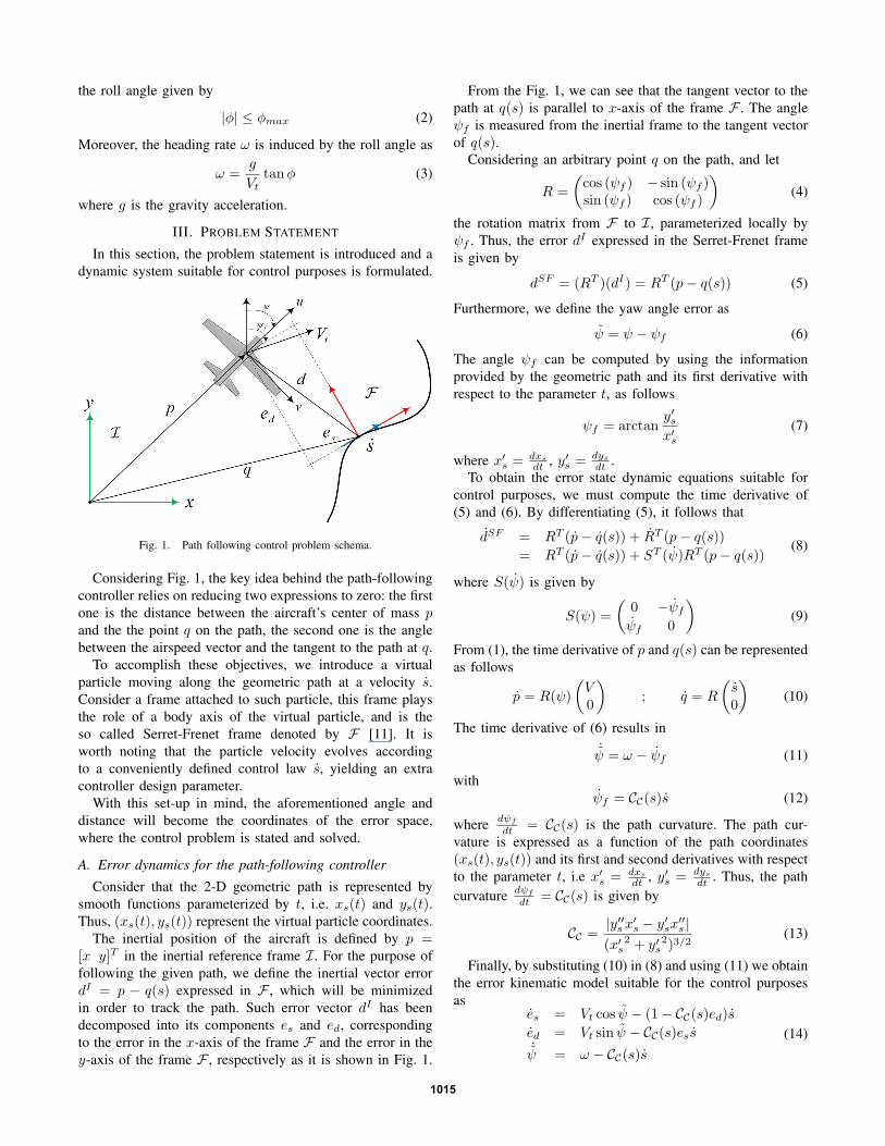
Fig. 1. Path following control problem schema.

Considering Fig. 1, the key idea behind the path-following

controller relies on reducing two expressions to zero: the first

one is the distance between the aircraft’s center of mass pand the the point q on the path, the second one is the angle

between the airspeed vector and the tangent to the path at q.

To accomplish these objectives, we introduce a virtual

particle moving along the geometric path at a velocity s.Consider a frame attached to such particle, this frame plays

the role of a body axis of the virtual particle, and is the

so called Serret-Frenet frame denoted by F [11]. It is

worth noting that the particle velocity evolves according

to a conveniently defined control law s, yielding an extra

controller design parameter.

With this set-up in mind, the aforementioned angle and

distance will become the coordinates of the error space,

where the control problem is stated and solved.

A. Error dynamics for the path-following controller

Consider that the 2-D geometric path is represented by

smooth functions parameterized by t, i.e. xs(t) and ys(t).Thus, (xs(t), ys(t)) represent the virtual particle coordinates.

The inertial position of the aircraft is defined by p =[x y]T in the inertial reference frame I. For the purpose of

following the given path, we define the inertial vector error

dI = p − q(s) expressed in F , which will be minimized

in order to track the path. Such error vector dI has been

decomposed into its components es and ed, corresponding

to the error in the x-axis of the frame F and the error in the

y-axis of the frame F , respectively as it is shown in Fig. 1.

From the Fig. 1, we can see that the tangent vector to the

path at q(s) is parallel to x-axis of the frame F . The angle

ψf is measured from the inertial frame to the tangent vector

of q(s).Considering an arbitrary point q on the path, and let

R =

(

cos (ψf ) − sin (ψf )sin (ψf ) cos (ψf )

)

(4)

the rotation matrix from F to I, parameterized locally by

ψf . Thus, the error dI expressed in the Serret-Frenet frame

is given by

dSF = (RT )(dI) = RT (p− q(s)) (5)

Furthermore, we define the yaw angle error as

ψ = ψ − ψf (6)

The angle ψf can be computed by using the information

provided by the geometric path and its first derivative with

respect to the parameter t, as follows

ψf = arctany′sx′s

(7)

where x′s = dxs

dt , y′s = dys

dt .

To obtain the error state dynamic equations suitable for

control purposes, we must compute the time derivative of

(5) and (6). By differentiating (5), it follows that

dSF = RT (p− q(s)) + RT (p− q(s))

= RT (p− q(s)) + ST (ψ)RT (p− q(s))(8)

where S(ψ) is given by

S(ψ) =

(

0 −ψfψf 0

)

(9)

From (1), the time derivative of p and q(s) can be represented

as follows

p = R(ψ)

(

V0

)

; q = R

(

s0

)

(10)

The time derivative of (6) results in

˙ψ = ω − ψf (11)

with

ψf = CC(s)s (12)

wheredψf

dt = CC(s) is the path curvature. The path cur-

vature is expressed as a function of the path coordinates

(xs(t), ys(t)) and its first and second derivatives with respect

to the parameter t, i.e x′s = dxs

dt , y′s = dys

dt . Thus, the path

curvaturedψf

dt = CC(s) is given by

CC =|y′′sx

′s − y′sx

′′s |

(x′s2 + y′s

2)3/2(13)

Finally, by substituting (10) in (8) and using (11) we obtain

the error kinematic model suitable for the control purposes

ases = Vt cos ψ − (1 − CC(s)ed)s

ed = Vt sin ψ − CC(s)ess˙ψ = ω − CC(s)s

(14)

1015

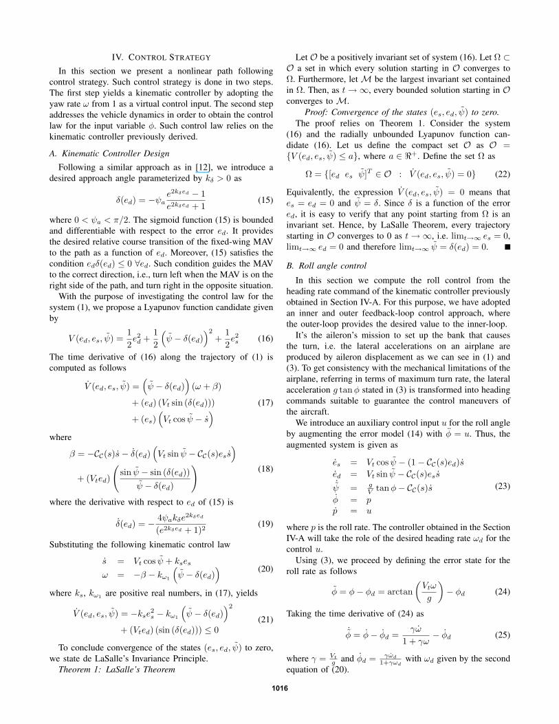
IV. CONTROL STRATEGY

In this section we present a nonlinear path following

control strategy. Such control strategy is done in two steps.

The first step yields a kinematic controller by adopting the

yaw rate ω from 1 as a virtual control input. The second step

addresses the vehicle dynamics in order to obtain the control

law for the input variable φ. Such control law relies on the

kinematic controller previously derived.

A. Kinematic Controller Design

Following a similar approach as in [12], we introduce a

desired approach angle parameterized by kδ > 0 as

δ(ed) = −ψae2kδed − 1

e2kδed + 1(15)

where 0 < ψa < π/2. The sigmoid function (15) is bounded

and differentiable with respect to the error ed. It provides

the desired relative course transition of the fixed-wing MAV

to the path as a function of ed. Moreover, (15) satisfies the

condition edδ(ed) ≤ 0 ∀ed. Such condition guides the MAV

to the correct direction, i.e., turn left when the MAV is on the

right side of the path, and turn right in the opposite situation.

With the purpose of investigating the control law for the

system (1), we propose a Lyapunov function candidate given

by

V (ed, es, ψ) =1

2e2d +

1

2

(

ψ − δ(ed))2

+1

2e2s (16)

The time derivative of (16) along the trajectory of (1) is

computed as follows

V (ed, es, ψ) =(

ψ − δ(ed))

(ω + β)

+ (ed) (Vt sin (δ(ed)))

+ (es)(

Vt cos ψ − s)

(17)

where

β = −CC(s)s− δ(ed)(

Vt sin ψ − CC(s)ess)

+ (Vted)

(

sin ψ − sin (δ(ed))

ψ − δ(ed)

)

(18)

where the derivative with respect to ed of (15) is

δ(ed) = −4ψakδe

2kδed

(e2kδed + 1)2(19)

Substituting the following kinematic control law

s = Vt cos ψ + kses

ω = −β − kω1

(

ψ − δ(ed))

(20)

where ks, kω1are positive real numbers, in (17), yields

V (ed, es, ψ) = −kse2s − kω1

(

ψ − δ(ed))2

+ (Vted) (sin (δ(ed))) ≤ 0(21)

To conclude convergence of the states (es, ed, ψ) to zero,

we state de LaSalle’s Invariance Principle.

Theorem 1: LaSalle’s Theorem

Let O be a positively invariant set of system (16). Let Ω ⊂O a set in which every solution starting in O converges to

Ω. Furthermore, let M be the largest invariant set contained

in Ω. Then, as t→ ∞, every bounded solution starting in Oconverges to M.

Proof: Convergence of the states (es, ed, ψ) to zero.

The proof relies on Theorem 1. Consider the system

(16) and the radially unbounded Lyapunov function can-

didate (16). Let us define the compact set O as O =V (ed, es, ψ) ≤ a, where a ∈ ℜ+. Define the set Ω as

Ω = [ed es ψ]T ∈ O : V (ed, es, ψ) = 0 (22)

Equivalently, the expression V (ed, es, ψ) = 0 means that

es = ed = 0 and ψ = δ. Since δ is a function of the error

ed, it is easy to verify that any point starting from Ω is an

invariant set. Hence, by LaSalle Theorem, every trajectory

starting in O converges to 0 as t→ ∞, i.e. limt→∞ es = 0,

limt→∞ ed = 0 and therefore limt→∞ ψ = δ(ed) = 0.

B. Roll angle control

In this section we compute the roll control from the

heading rate command of the kinematic controller previously

obtained in Section IV-A. For this purpose, we have adopted

an inner and outer feedback-loop control approach, where

the outer-loop provides the desired value to the inner-loop.

It’s the aileron’s mission to set up the bank that causes

the turn, i.e. the lateral accelerations on an airplane are

produced by aileron displacement as we can see in (1) and

(3). To get consistency with the mechanical limitations of the

airplane, referring in terms of maximum turn rate, the lateral

acceleration g tanφ stated in (3) is transformed into heading

commands suitable to guarantee the control maneuvers of

the aircraft.

We introduce an auxiliary control input u for the roll angle

by augmenting the error model (14) with φ = u. Thus, the

augmented system is given as

es = Vt cos ψ − (1 − CC(s)ed)s

ed = Vt sin ψ − CC(s)ess˙ψ = g

V tanφ− CC(s)s

φ = pp = u

(23)

where p is the roll rate. The controller obtained in the Section

IV-A will take the role of the desired heading rate ωd for the

control u.

Using (3), we proceed by defining the error state for the

roll rate as follows

φ = φ− φd = arctan

(

Vtω

g

)

− φd (24)

Taking the time derivative of (24) as

˙φ = φ− φd =

γω

1 + γω− φd (25)

where γ = Vt

g and φd = γωd

1+γωdwith ωd given by the second

equation of (20).

1016

In order to obtain the control u, we propose the total

candidate Lyapunov function given by

W (φ,˙φ, ed, es, ψ) =

λ

2(φ)2 +

˙φ(φ)

+q

2λ˙φ2 +

1

2e2s

+1

2e2d +

1

2

(

ψ − δ(ed))2

(26)

Where λ > 0 and q > 1 are free parameters to be chosen.

Using the controllers (20), the time derivative of (26) along

the trajectory of (23) is given by

W (φ,˙φ, ed, es, ψ) = u

( q

λ˙φ+ φ

)

+ λφ˙φ+

˙φ2

− kω1

(

ψ − δ(ed))2

− kse2s

+ (Vted) (sin (δ(ed)))

(27)

Consider the control input

u = −kpφ− kd˙φ (28)

where kp and kd are positive real numbers. Then, substituting

(28) in (27) it leads to

W (φ,˙φ, ed, es, ψ) = −kpφ

2 −

(

kdq

λ− 1

)

˙φ2

− kω1

(

ψ − δ(ed))2

− kse2s

+ (Vted) (sin (δ(ed)))

(29)

Using the same procedure of the previous section, it leads to

W (φ,˙φ, ed, es, ψ) < 0 provided that

kpqλ +kd−λ = 0, kd >

λq . Therefore, the control law (28) makes the convergence of

the states to ed → 0, es → 0, ψ → 0 and ω → ωd.

V. SIMULATION RESULTS AND EXPERIMENTAL

PLATFORM

The simulation platform MAV3DSim is based on the

open-source simulator CRRCSim [13], which was created

based on a simulator (BASIC) developed by the National

Aeronautics and Space Administration (NASA). Our simu-

lator MAV3DSim implements the complete nonlinear model

in six degrees of freedom (6DoF). In addition, we have

include aerodynamic forces generated by the aircraft control

surfaces in order to to incorporate the 6DoF kinematic model.

MAV3DSim has the capability to simulate the behavior of

a specific model plane, additionally the user can change the

aircraft aerodynamic coefficients. It also has a 3D represen-

tation to visualize the position and orientation of the plane.

Regarding communication capacities, one of the main

advantages is that the user can establish a communication

link with another computer via UDP protocol, and thereby

send and receive information under a standard package of

data used by the MNAV100CA Robotics Sensor Suites [14].

It means that MAV3DSim can simulate the sending data in

a similar manner as does the aircraft. Such data includes

the information provided by the IMU (attitude and angular

rate), GPS (global position and velocities) and pitot tube

(airspeed). Furthermore, it can receive control commands for

the thrust and the control surfaces such as aileron, elevator

and rudder.

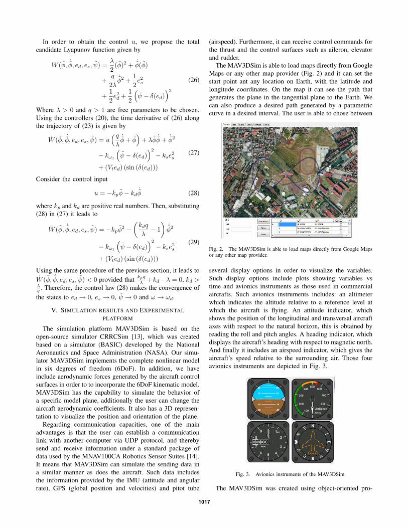
The MAV3DSim is able to load maps directly from Google

Maps or any other map provider (Fig. 2) and it can set the

start point ant any location on Earth, with the latitude and

longitude coordinates. On the map it can see the path that

generates the plane in the tangential plane to the Earth. We

can also produce a desired path generated by a parametric

curve in a desired interval. The user is able to chose between

Fig. 2. The MAV3DSim is able to load maps directly from Google Mapsor any other map provider.

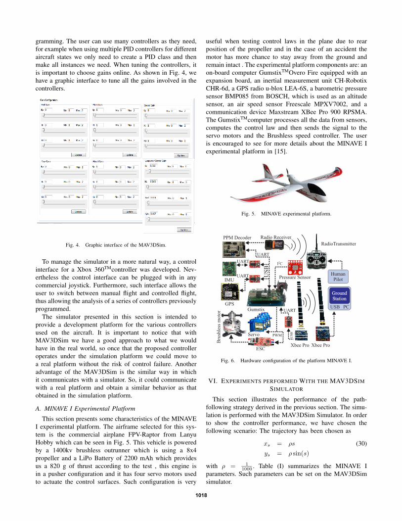
several display options in order to visualize the variables.

Such display options include plots showing variables vs

time and avionics instruments as those used in commercial

aircrafts. Such avionics instruments includes: an altimeter

which indicates the altitude relative to a reference level at

which the aircraft is flying. An attitude indicator, which

shows the position of the longitudinal and transversal aircraft

axes with respect to the natural horizon, this is obtained by

reading the roll and pitch angles. A heading indicator, which

displays the aircraft’s heading with respect to magnetic north.

And finally it includes an airspeed indicator, which gives the

aircraft’s speed relative to the surrounding air. Those four

avionics instruments are depicted in Fig. 3.

Fig. 3. Avionics instruments of the MAV3DSim.

The MAV3DSim was created using object-oriented pro-

1017

gramming. The user can use many controllers as they need,

for example when using multiple PID controllers for different

aircraft states we only need to create a PID class and then

make all instances we need. When tuning the controllers, it

is important to choose gains online. As shown in Fig. 4, we

have a graphic interface to tune all the gains involved in the

controllers.

Fig. 4. Graphic interface of the MAV3DSim.

To manage the simulator in a more natural way, a control

interface for a Xbox 360TMcontroller was developed. Nev-

ertheless the control interface can be plugged with in any

commercial joystick. Furthermore, such interface allows the

user to switch between manual flight and controlled flight,

thus allowing the analysis of a series of controllers previously

programmed.

The simulator presented in this section is intended to

provide a development platform for the various controllers

used on the aircraft. It is important to notice that with

MAV3DSim we have a good approach to what we would

have in the real world, so once that the proposed controller

operates under the simulation platform we could move to

a real platform without the risk of control failure. Another

advantage of the MAV3DSim is the similar way in which

it communicates with a simulator. So, it could communicate

with a real platform and obtain a similar behavior as that

obtained in the simulation platform.

A. MINAVE I Experimental Platform

This section presents some characteristics of the MINAVE

I experimental platform. The airframe selected for this sys-

tem is the commercial airplane FPV-Raptor from Lanyu

Hobby which can be seen in Fig. 5. This vehicle is powered

by a 1400kv brushless outrunner which is using a 8x4

propeller and a LiPo Battery of 2200 mAh which provides

us a 820 g of thrust according to the test , this engine is

in a pusher configuration and it has four servo motors used

to actuate the control surfaces. Such configuration is very

useful when testing control laws in the plane due to rear

position of the propeller and in the case of an accident the

motor has more chance to stay away from the ground and

remain intact . The experimental platform components are: an

on-board computer GumstixTMOvero Fire equipped with an

expansion board, an inertial measurement unit CH-Robotix

CHR-6d, a GPS radio u-blox LEA-6S, a barometric pressure

sensor BMP085 from BOSCH, which is used as an altitude

sensor, an air speed sensor Freescale MPXV7002, and a

communication device Maxstream XBee Pro 900 RPSMA.

The GumstixTMcomputer processes all the data from sensors,

computes the control law and then sends the signal to the

servo motors and the Brushless speed controller. The user

is encouraged to see for more details about the MINAVE I

experimental platform in [15].

Fig. 5. MINAVE experimental platform.

IMU

GPS

Xbee Pro

Radio ReceiverPPM Decoder

PC

Ground

Station

USB

Human

PilotPressure Sensor

Gumstix

Xbee Pro

US

BUART

UART

UART

US

B

UART

PWM

I2C

Servo

ESC

Bru

sh

less m

oto

r

RadioTransmitter

Fig. 6. Hardware configuration of the platform MINAVE I.

VI. EXPERIMENTS PERFORMED WITH THE MAV3DSIM

SIMULATOR

This section illustrates the performance of the path-

following strategy derived in the previous section. The simu-

lation is performed with the MAV3DSim Simulator. In order

to show the controller performance, we have chosen the

following scenario: The trajectory has been chosen as

xs = ρs (30)

ys = ρ sin(s)

with ρ = 1

1000. Table (I) summarizes the MINAVE I

parameters. Such parameters can be set on the MAV3DSim

simulator.

1018

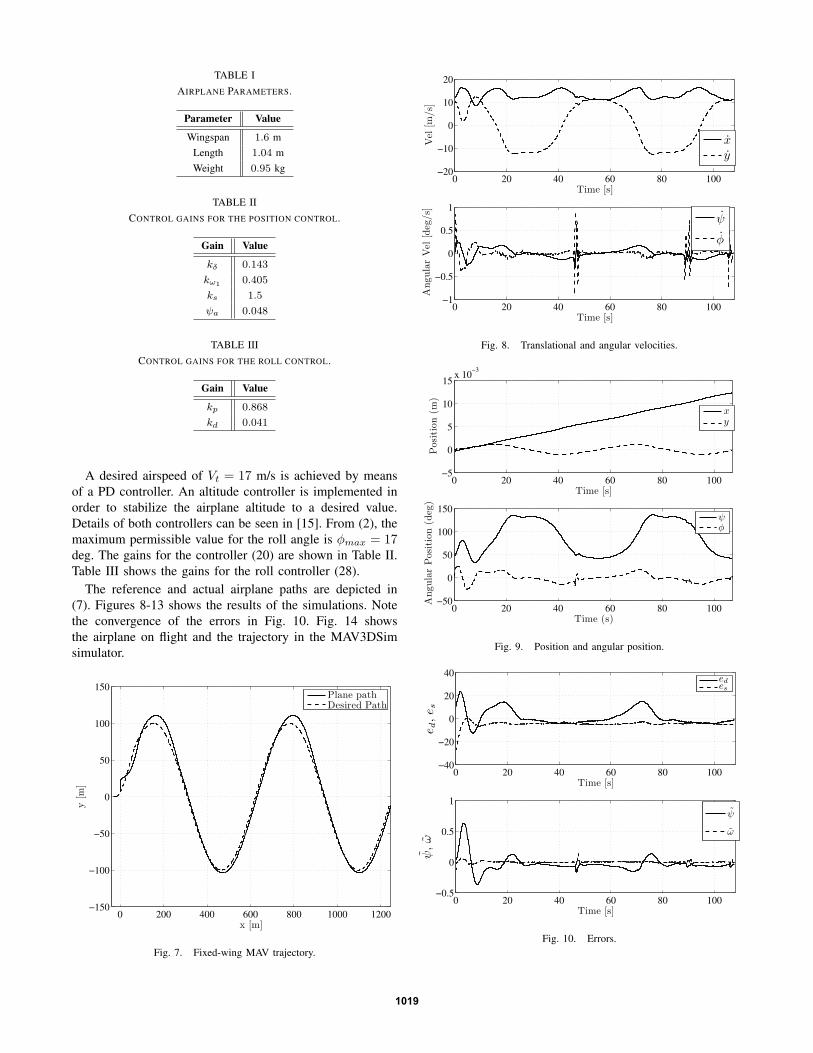
TABLE I

AIRPLANE PARAMETERS.

Parameter Value

Wingspan 1.6 m

Length 1.04 m

Weight 0.95 kg

TABLE II

CONTROL GAINS FOR THE POSITION CONTROL.

Gain Value

kδ 0.143

kω10.405

ks 1.5

ψa 0.048

TABLE III

CONTROL GAINS FOR THE ROLL CONTROL.

Gain Value

kp 0.868

kd 0.041

A desired airspeed of Vt = 17 m/s is achieved by means

of a PD controller. An altitude controller is implemented in

order to stabilize the airplane altitude to a desired value.

Details of both controllers can be seen in [15]. From (2), the

maximum permissible value for the roll angle is φmax = 17deg. The gains for the controller (20) are shown in Table II.

Table III shows the gains for the roll controller (28).

The reference and actual airplane paths are depicted in

(7). Figures 8-13 shows the results of the simulations. Note

the convergence of the errors in Fig. 10. Fig. 14 shows

the airplane on flight and the trajectory in the MAV3DSim

simulator.

0 200 400 600 800 1000 1200−150

−100

−50

0

50

100

150

x [m]

y[m

]

Plane pathDesired Path

Fig. 7. Fixed-wing MAV trajectory.

0 20 40 60 80 100−20

−10

0

10

20

Vel

[m/s]

Time [s]

xy

0 20 40 60 80 100−1

−0.5

0

0.5

1

Time [s]

Angula

rV

el[d

eg/s]

ψ

φ

Fig. 8. Translational and angular velocities.

0 20 40 60 80 100−5

0

5

10

15x 10

−3

Posi

tion

(m)

Time [s]

xy

0 20 40 60 80 100−50

0

50

100

150

Time (s)

Angula

rP

osi

tion

(deg

)

ψφ

Fig. 9. Position and angular position.

0 20 40 60 80 100−40

−20

0

20

40

Time [s]

e d,e s

edes

0 20 40 60 80 100−0.5

0

0.5

1

Time [s]

ψ,ω

ψ

ω

Fig. 10. Errors.

1019

0 20 40 60 80 100−40

−20

0

20

Time [s]

s

0 20 40 60 80 100−0.4

−0.2

0

0.2

0.4

Time [s]

ωd

Fig. 11. Controllers.

0 20 40 60 80 100−0.25

−0.2

−0.15

−0.1

−0.05

0

0.05

0.1

0.15

0.2

0.25

Time [s]

u

Fig. 12. Control u.

0 20 40 60 80 1000

100

200

300

400

500

600

700

800

900

Curv

atu

re

Time[s]

Fig. 13. Curvature for the trajectory generated by (30).

Fig. 14. Airplane in the simulator tracking a path.

VII. CONCLUDING REMARKS

This paper presented a nonlinear path-following strategy

for a fixed-wing MAV based on the Lyapunov theory. The

controller has been tested in simulation showing a good

performance. Such controller relies on accurate knowledge

of vehicle dynamics. It is worth mentioning that although

the controller was designed using a reduced model of the

airplane, the tests carried out in the simulator, worked with

the complete nonlinear aircraft model. This fact leads to the

effectiveness of the proposed controller on a real experimen-

tal platform. On the other hand, the simulator MAV3DSim

proves to be a great candidate for implementation of dif-

ferent controllers. Future work will address the problem of

robustness in presence of wind gusts. Also, the proposed

controller will be implemented on the MINAVE I experi-

mental platform, in order to test the effectiveness of such

algorithm. In the future, other type of aerial vehicles such

as quad-rotors or coaxial helicopters, could be implemented

using the simulator MAV3DSim.

REFERENCES

[1] N. Aouf, B. Boulet, and R. Botez, “Vector field path followingfor small unmanned air vehicles,” in Proc. IEEE American Control

Conference (ACC’2002), Anchorage, AK, May 2002, pp. 4439–4442vol.6.

[2] M. Niculescu, “Lateral track control law for aerosonde uav,” in 39th

AIAA Aerospace Sciences Meeting and Exhibit, Reno, NV, Jan. 2001,p. AIAA 20010016.

[3] D. R. Nelson, D. B. Barber, T. W. McLain, and R. W. Beard, “Imagemoments: a general and useful set of features for visual servoing,”IEEE Trans. on Robotics, vol. 23, no. 3, pp. 512–529, June, 2007.

[4] R. Wei and R. W. Beard, “Trajectory tracking for unmanned air vehi-cles with velocity and heading rate constraints,” IEEE Transactions on

Control Systems Technology, vol. 12, no. 5, pp. 706–716, Sept. 2004.[5] D. R. Nelson, D. B. Barber, T. W. McLain, and R. W. Beard, “Vector

field path following for small unmanned air vehicles,” in Proc. IEEE

American Control Conference (ACC’2006), Minneapolis, Minnesota,USA, Jun. 2006, pp. 5788–5794.

[6] O. Khatib, “Real-time obstacle avoidance for manipulators and mobilerobots,” in Proc. IEEE International Conference on Robotics and

Automation (ICRA’1985), St. Louis, Missouri, May 1985, p. 500505.[7] K. Sigurd and J. P. How, “Uav trajectory design using total field

collision avoidance,” in Proc. of the AIAA Guidance, Navigation, and

Control Conference, Austin, TX, Aug. 2003.[8] Y. Koren and J. Borenstein, “Potential field methods and their inherent

limitations for mobile robot navigation,” in Proc. IEEE International

Conference on Robotics and Automation (ICRA’1991), Sacramento,California, Apr. 1991, pp. 1398–1404.

1020

[9] F. Allgower and A. Zheng, Nonlinear Model Predictive Control.Birkhauser, 2000.

[10] H. Chitsaz and S. LaValle, “Time-optimal paths for a dubins airplane.”in Proc. IEEE Conference on Decision and Control (CDC’2007), NewOrleans, LA, USA, Dec. 2007, pp. 2379–2384.

[11] A. Micaelli and C. Samson, “Trajectory tracking for unicycle-type andtwo-steering-wheels mobile robots,” INRIA, Tech. Rep. 2097, 1993.

[12] L. Lapierre and D. Soetanto, “Nonlinear path-following control of anauv,” Ocean Engineering, vol. 1112, no. 34, p. 17341744, 2007.

[13] O. Source. (2013) Crrcsim. [Online]. Available: http://sourceforge.net/apps/mediawiki/crrcsim/

[14] MNAV100CA User’s Manual, Crossbow Technology, Inc, 1996.[15] I. Lugo-Cardenas, “Nonlinear control of a mini aereal vehicle for

trayectory tracking,” Master’s thesis, Centre for Research and Ad-vanced Studies, Av. Instituto Politecnico Nacional 2508, Mexico City,Mexico, 2013.

1021