A New Study of the Mediterranean Outflow, Air Sea Interactions, and Meddies Using Multisensor Data

A New Study of the Mediterranean Outflow, Air–Sea Interactions, and Meddies UsingMultisensor Data

XIAO-HAI YAN* AND YOUNG-HEON JO

Graduate College of Marine Studies, University of Delaware, Newark, Delaware

W. TIMOTHY LIU

Jet Propulsion Laboratory, California Institute of Technology, Pasadena, California

MING-XIA HE

Ocean Remote Sensing Institute, Ocean University of Qingdao, Qingdao, China

(Manuscript received 29 November 2004, in final form 7 September 2005)

ABSTRACT

Previous studies of the Mediterranean Sea outflow and meddies (O&M) were limited by the poor spatialand temporal resolution of conventional in situ observations as well as the confinement of satellite obser-vations to the ocean’s surface. Accordingly, little is known about the formation and transport of meddiesand the spatial and temporal variation of O&M trajectories, which are located, on average, at a depth of1000 m. However, a new remote sensing method has been developed by the authors to observe and studythe O&M through unique approaches in satellite multisensor data integration analyses. Satellite altimeter,scatterometer, infrared satellite imagery, and XBT data were used to detect and calculate the trajectoriesand the relative transport of the O&M (January 1993–December 2002). Two experiments [covering 1993–95: A Mediterranean Undercurrent Seeding Experiment (AMUSE) and Structures des Echanges Mer–Atmosphère, Propriétés des Hétérogénéités Océaniques: Recherche Expérimentale (SEMAPHORE)] andXBT temperature measurements were used to directly validate the method presented herein. The monthlymean features derived from floats and XBTs for multiple meddies and the results of the presented methodwere significantly correlated based on a statistical chi-square test. In addition, the complex singular valuedecomposition method was used to identify the propagating features and their phase speeds. It was foundthat saltier water from the Mediterranean Sea was transported into the North Atlantic Ocean over the Straitof Gibraltar in boreal spring and summer relative to boreal autumn and winter. Streamfunctions usingaltimetry, and time–frequency energy distributions using the Hilbert–Huang transform, were computed toevaluate the meddy interactions with the sea surface variation. Since the O&M play a significant role incarrying salty water from the Mediterranean Sea into the Atlantic, such new knowledge about their tra-jectories, transport, and life histories is important to the understanding of their mixing and interaction withNorth Atlantic water. This may lead to a better understanding of the global ocean circulation and globalclimate change.

1. Introduction

One of the most interesting and prominent featuresof the North Atlantic Ocean is the salt tongues origi-

nating from an exchange flow between the Mediterra-nean Sea and the Atlantic through the Strait of Gibral-tar. The Mediterranean outflow through the strait isdenser than Atlantic water because of its higher saltcontent. Evaporation in the Mediterranean Sea raisesthe salinity to around 38.4 psu, as compared with 36.4psu in the eastern North Atlantic. After leaving thestrait under the incoming, lighter North Atlantic water,the Mediterranean outflow sinks and turns to the right,because of the Coriolis force, following the continentalslope off Spain and Portugal. Eventually, this waterleaves the coast and spreads into the middle North At-

* Additional affiliation: Ocean University of Qingdao, Qingdao,China.

Corresponding author address: Xiao-Hai Yan, Graduate Col-lege of Marine Studies, University of Delaware, Newark, DE19716.E-mail: [email protected]

APRIL 2006 Y A N E T A L . 691

© 2006 American Meteorological Society

JPO2873

lantic, forming a tongue of salty water. This generatesclockwise-rotating eddies. These Mediterranean eddies,or meddies (McDowell and Rossby 1978) as they areoften called, are rapidly rotating double-convex lensesthat contain a warm, highly saline core of Mediterra-nean water 200–1000 m thick. Relative to the back-ground water in the Canary Basin, meddy salinity andtemperature anomalies can be 1 psu and 2°–4°C higher,respectively (Bower et al. 1997; Richardson et al. 2000).Because of the water differences between a meddy andthe North Atlantic, isopycnal amplitude reaches 6 cm(Stammer et al. 1991; Tychensky and Carton 1998). Ameddy has a typical diameter of approximately 100 kmand, on average, is located at a depth of 1000 m. Mostmeddy observations have been found in the CanaryBasin (Armi and Zenk 1984; Käse and Zenk 1987) andin the eastern North Atlantic (Armi and Stommel 1983;Pingree and Le Cann 1993; Bower et al. 1997).

Generally speaking, most remotely sensed oceano-graphic observations are confined to either the sea sur-face or to the upper mixed layer, but this limitation isnot always true. Yan et al. (1990, 1991a,b) and Yan andOkubo (1992) developed methods to infer the upper-ocean mixed layer depths from multisensor satellitedata. Furthermore, Stammer et al. (1991) applied Geo-sat Exact Repeat Mission (GERM) altimeter data toinvestigate the possible surface signal of meddies. Theycompared the dynamic topography calculated from hy-drographic data with samples from an eddy-resolvingstation network in the Iberian Basin. Although theywere unable to detect meddies from space alone (in theabsence of accompanying in situ data), they identifiedthe possible surface meddy signals using both GERMaltimeter data and hydrographic data. Similarly, Tok-makian and Challenor (1993) also reported that indi-vidual eddies or meddies cannot be identified usingGERM altimeter data, but the Azores Current could be.

The possible surface meddy signals in the altimeterdata were distinguishable from the background (e.g.,fronts, currents, and eddies) field determined from hy-drographic data. The formation and early stages of de-velopment of anticyclonic mesoscale eddies with a coreof slope water were observed in a study by Pingree andLe Cann (1992). One of these slope water oceanic ed-dies (“swoddie”) was seen in infrared (IR) satellite im-agery. Pingree and Le Cann (1993) also showed evi-dence of a shallow meddy (smeddy) at 700-m depth onthe southern Tagus Abyssal Plain from IR satellite im-agery. However, IR imagery only enables one to moni-tor the early stage of the possible meddies, when thereis a sea surface temperature (SST) gradient, and whenmeddies are located in a shallow region. The earlystage, which occurs close to the sharp dropoff of the

continental shelf, can be distinguished from the laterstages by the location of the formation of the meddies.Oliveira et al. (2000) showed these eddylike featuresusing a sequence of six SST images and altimetry dataand compared these features with float data. Theyfound that the IR image of the meddies during thewinter/spring is clearer than other seasons when coastalupwelling is relaxed.

We hereby report a new method to study the Medi-terranean outflow and meddies (O&M) by analysis ofaltimeter, scatterometer, IR satellite imagery, and ex-pendable bathythermography (XBT) data. We com-pute the vertical sea level difference: �� Total ��UL � ��Total � (��T � ��S � ��W), where ��Total is thedeviation of the sea surface topography of the wholevertical water column, which can be measured by al-timetry, and ��UL is the sea surface variation in the up-per layer (400 m) due to thermal expansion ��T, saltexpansion ��S, and the wind stress ��W. Because it isimpossible to decompose the sea surface heightanomaly into each corresponding signal, such as ��T, ��S,and ��W, we estimated them using individual measure-ments, and then removed the signals of ��T, ��S, and ��Wfrom the total sea level variation ��Total. Therefore, weconsider the rest of the signal as the meddy signals|��|, and this sea level difference, |��|, is used to dis-tinguish meddy signals from the background field in theupper layer. Thus, the meddy signals are not necessarilyindividual meddies, but actually multiple meddies at a400-m isopycnal surface.

It is worth noting that our results differ from those ofStammer et al. (1991) and others referenced above. Toremove the upper-layer variation (include the Azoresfront) from the many other signals in the altimeter data,we differentiated the surface meddy signals from thethermal-, salinity-, and wind-induced sea level varia-tions of the upper layer (0–400 m). By removing the othersignals in the altimeter data, one can, thus, identify thesignal of the O&M. In addition, one can even monitorthe meddies, not only in the early stages near the con-tinental shelf, but also in the later stages at greaterdistances from their origin. The improved methodologydeveloped in this study also permits a longer time scale(because our data record length is longer) than GERMaltimeter data and achieves a higher degree of accuracythan those from earlier studies.

The rest of this paper is organized as follows: themethod and data are described in section 2. We thenintroduce the approach for removing the signals of theupper-layer variation in section 3, and we present ourO&M signal and validation in section 4. In section 5,the following studies are presented the spatial and tem-poral variations of the meddies |��| using complex sin-

692 J O U R N A L O F P H Y S I C A L O C E A N O G R A P H Y VOLUME 36

gular value decomposition analysis, the relative trans-port of the Mediterranean outflow, and the interactionsbetween sea level variation determined from thestreamfunction and the meddies measured by thefloats. Section 6 presents the conclusions.

2. Methods and data

a. Integrated multisensor data analysis (IMSDA)

We used the following algorithm to estimate themeddy signals:

��T, S, W, X, t� � ��Total�T, S, W, X, t� �1K

K

�Total�T, S, W, X, t�� UL�T, S, W, X, t� �

1K

K

�UL�T, S, W, X, t��Total � ��UL, �1�

where

��UL � ��T�T, X, t� �1K

K

�T�T, X, t�� S�S, X, t� �1K

K

�S�S, X, t�� W�W, X, t� �

1K

K

�W�W, X, t�� 2�

and

��UL � ��T � ��S � ��W, �3�

where ��Total is the deviation of the sea surface topog-raphy, �Total, after removing the long-term mean, whichcan be measured by satellite altimetry. In addition, T, S,W, X, and t represent temperature, salinity, wind, space,and time in months (K � 120 months from January1993 to December 2002), respectively. The ��UL varia-tion is due to ��T, ��S, and ��W, which can be estimatedfrom temperature measurements from IR satellite im-agery and XBTs, salinity measurements from Levitusand Boyer (1994, hereinafter Levitus 94), and scatter-ometer data from the European Remote Sensing Satel-lites-1 and -2 (ERS-1/2), the National Aeronautics andSpace Administration (NASA) Scatterometer (NSCAT),and the NASA Quick Scatterometer (QuikSCAT), re-spectively. A time series of gridded monthly values ofthe O&M signals with 18-km resolution was developed.This resolution is high enough to resolve mesoscale fea-tures [e.g., meddy’s horizontal scale (100-km diam-eter)].

b. Coupled pattern analysis

Coupled pattern analysis (CPA) provides anothermeans of matching patterns for two separate time-dependent fields, provided the processes underlying thetwo are simply and directly related. In essence, they area means of deducing matched pairs of spatial patterns,one for each field, that have a high temporal correla-tion. This property makes it more attractive than de-riving the empirical orthogonal function (EOF) modesof each of the two fields separately and comparing

them, mode by mode. This method is effective, thoughthe purely statistical nature of the analysis and the em-pirical nature of the basis functions for the two fieldsmean that the EOF modes of the two fields may not benecessarily related to each other. CPA has been used inanalyzing climate data (Bretherton et al. 1992), andmatching the patterns of variability of SST and atmo-spheric pressure (Peng and Fyfe 1996; Wallace et al.1992).

CPA analysis is similar to EOF analysis (Leulietteand Wahr 1999) in that the two fields are decomposedinto orthonormal modes:

f �x, t� � k�1

M

�k�t�uk�x� and �4�

g�x, t� � k�1

M

�k�t��k�x�, �5�

where u and � are the spatially dependent function off(x, t) and g(x, t), respectively. Here M is the number ofspatial points x.

We defined f(x, t) as ��T and g(x, t) as the SSTanomaly SST� in this study. By determining a regres-sion coefficient between f(x, t) and g(x, t), we estimateda new thermal steric height anomaly from SST�. Thedetails of the application of this methodology are dis-cussed in section 3.

c. Complex singular value decomposition (CSVD)

Barnett (1983) applied complex EOF (CEOF) analy-sis using a covariance matrix to investigate the interac-tion of the monsoon and trade wind systems in thePacific Ocean. In this study, we used CSVD, for which


the covariance matrix is not needed. Using CSVD, onecan calculate not only the eigenvalues and eigenvectors,but also the spatial amplitudes, and spatial and tempo-ral phase functions (Susanto et al. 1998). Susanto et al.(1998) defined the spatial �n(t) and temporal n(t)phase function as shown in (6) and we used that tostudy the propagating phases of the O&M:

�n�t� � arctan�Im�An�t��Re�An�t�� and

�n�t� � arctan�Im�Bn�t��Re�Bn�t��, �6�

where An and Bn are the spatial and temporal complexprincipal components, respectively, and t is time.

d. Hilbert–Huang transform (HHT) and spectra(HHS)

The fundamental idea of time–frequency analysis isto understand and describe situations where the fre-quency component of a signal is changing in time. Theextrinsic mode decomposition (EMD) method is a gen-eral method of time–frequency analysis, which is appli-cable to nonlinear and nonstationary signals. Since thedecomposition is based on the local characteristic timescale of the data, it is applicable to nonlinear and non-stationary processes. With the Hilbert transform, theintrinsic mode functions (IMFs) yield instantaneousfrequencies, as functions of time that give sharp iden-tification of embedded structures. The main conceptualinnovation in this approach is the introduction of theinstantaneous frequencies for complicated datasets,which eliminate the need for spurious harmonics to rep-resent nonlinear and nonstationary signals. The essenceof the EMD method is to identify the oscillatory modesby their characteristic time scales in the data empiri-cally and, then, decompose the data accordingly. Thedecomposition of the data into decomposed simplemode functions (SMFs) uses envelopes defined by thelocal maxima and minima separately. Once the extremaare identified, all the local maxima are connected by acubic spline as the upper envelope. The procedure isrepeated for the local minima to produce the lowerenvelope. The Hilbert spectrum was designed to applythe HHS to the SMF and construct the energy–fre-quency–time distribution (Huang et al. 1998). The Hil-bert-transformed series has the same amplitude andfrequency content as the original real data and alsoincludes phase information that depends on the phaseof the original data. The Hilbert transform is useful incalculating instantaneous attributes of a time series, es-pecially the amplitude and frequency. The instanta-

neous amplitude is the amplitude of the complex Hil-bert transform; the instantaneous frequency is the timerate of change of the instantaneous phase angle.

e. Sea level anomaly

The series of sea level anomalies (SLA) is obtainedfrom a complete reprocessing of Ocean TopographyExperiment (TOPEX)/Poseidon (T/P), Jason-1, andERS-1/2 satellite data (January 1993–December 2002).(Detailed information about the SLAs can be foundonline at ftp://ftp.cls.fr/pub/oceano/enact/msla/readme_MSLA_ENACT.htm.) The T/P instrumentwas replaced by Jason-1 in August 2002 after its orbitchange. ERS-2 is available from June 1996 to June2003. ERS-2 was then replaced by the EnvironmentalSatellite (ENVISAT). The SLAs were computed usingconventional repeat-track analysis. The SLAs are rela-tive to a 7-yr mean (January 1993–January 1999). Byremoving a 7-yr mean sea level height, we are able toremove the geoid from the altimeter measurements.Accordingly, the bathymetric effects on the altimetermeasurements are a minimum. A specific processing isperformed to get an ERS-2 mean consistent with a T/Pmean. The SLA is provided on a 1⁄3 Mercator grid.Resolutions in kilometers in latitude and longitude arethus identical and vary with the cosine of latitude (e.g.,from 37 km at the equator to 18.5 km at 60°N/S). Tomake the same grid points for the O&M signals usingEqs. (1)–(3), we interpolated the SLAs into a 18-kmspatial resolution, which is the same resolution as usedfor the Advanced Very High Resolution Radiometer(AVHRR) SST.

f. Thermal steric height (��T)

In order to estimate the sea level variation resultingfrom thermal expansion in the upper layer ��T, the seasurface height anomaly was calculated using monthlymean XBT data acquired from the Joint EnvironmentalData Analysis (JEDA) Center. This method integratedtemperatures through the water column to 400-mdepths from January 1993 to December 2002, that is,

��T � ��400

0

�T dz ��

K K �

�400

0

�T dz, �7�

where �T is the temperature difference between twodifferent depths (dz) and � is the thermal expansioncoefficient, which is calculated as a function of salinityS and water pressure P, based on empirical measure-ments (Wilson and Bradley 1966):


� � �10

�

�T��s, p�,

where �0 is the reference density and �� is the densitydifference between two layers. However, we found thatthe spatial resolution of XBT data (2° � 5° latitude–longitude) for the ��T was not high enough to resolvemesoscale features. To estimate the interpolation errorof the XBTs, we determined the correlation and rmsdifferences between optimum interpolation SST andSST derived from XBTs. Its correlation is O(0.96), andthe rms differences are 0.5°C, respectively. We believethat the spatial resolution of the XBT data before in-terpolation into 1° � 1° latitude–longitude is not aproblem, because ��T is supposed to estimate the sealevel variation for much larger spatial areas than that ofthe meddies.

Furthermore, in order to obtain better spatial reso-lution, we computed a new thermal steric height fromthe AVHRR SST data (18 km) after applying an em-pirical regression curve using CPA as demonstrated inthe next section. To do that, optimum interpolated seasurface temperature (OISST) with a spatial resolutionof a 1° grid, from January 1993 to December 2002, wasalso used. The OISST was obtained from the NationalOceanic and Atmospheric Administration/NationalCenters for Environmental Prediction (NOAA/NCEP).The monthly optimum interpolation (OI) fields werederived by a linear interpolation of the weekly OI fieldsto daily fields and then averaging the daily values overa month (Reynolds and Smith 1994). The sources ofOISST are based on the Comprehensive Ocean–Atmo-sphere Data Set and satellite observations. For theAVHRR (18-km resolution), we obtained the datafrom the Physical Oceanography Distributed ActiveArchive Center (PO.DAAC) AVHRR Oceans Path-finder (information online at ftp://podaac.jpl.nasa.gov/pub/sea_surface_temperature/avhrr/pathfinder/).

3. Removal of signals of upper-layer variationfrom ��Total for the O&M signal (|��|)

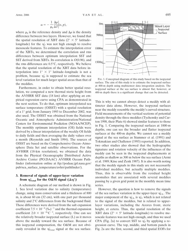
A schematic diagram of our method is shown in Fig.1. Sea level variation due to salinity (temperature)change, using mass conservation and a thickness of 800m, is about 60 cm (32 cm), with one part per thousandsalinity and 2°C differences from the background fluid.These differences were derived from the salt expansioncoefficient 7.5 � 10�4 (‰)�1 and the thermal expansioncoefficient 2.0 � 10�4°C�1, respectively. One can seethe relatively broader isopycnal surface (L) as it movesabove the meddy toward the sea surface. Because ofthis isopycnal compensation, the O&M are not obvi-ously revealed in the ��Total signal at the sea surface.

This is why we cannot always detect a meddy with al-timeter data alone. However, the isopycnal surfacesnear the meddy resemble the meddy’s curved structure.Field measurements of the vertical sections of potentialdensity through the three meddies (Tychensky and Car-ton 1998, their Plate 6) showed similar features to thosein Fig. 1. Comparing the isopycnal surfaces at 1000-mdepths, one can see the broader and flatter isopycnalsurfaces at the 400-m depths. We cannot see a meddysignal at the sea surface as Stammer et al. (1991) andTokmakian and Challenor (1993) reported. In addition,two other studies also showed that the hydrographicsignature and rotation velocity of the influences of themeddy can be seen in the isopycnal displacements atdepths as shallow as 300 m below the sea surface (Armiet al. 1989; Käse and Zenk 1987). It is also worth notingthat the meddy signals in this study are not necessarilyindividual meddies, but actually multiple meddies.Thus, this is observable from the residual heightanomalies that are associated with several meddiespassing by a given grid point in the monthly mean timeseries.

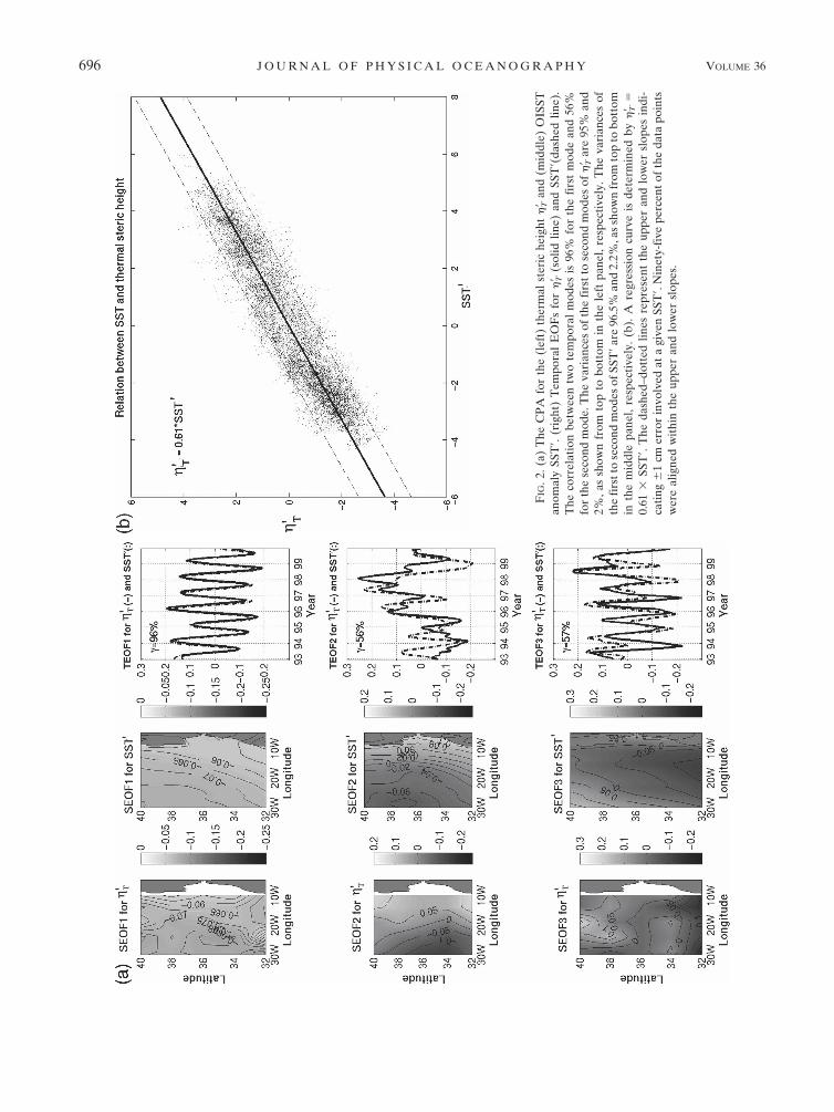
However, the question is how to remove the signalsof the sea surface variation in the upper-layer ��UL. Themajor component of the ��UL is ��T, which is not relatedto the signal of the meddies, but is related to upper-layer variations, including the Azores front, stericheight, et cetera. Thus, the spatial resolution of theXBT data (2° � 5° latitude–longitude) to resolve me-soscale features was not high enough, and thus we usedCPA (Fig. 2a) to convert SST to ��T by applying a re-gression curve. The top, middle, and bottom panels inFig. 2a are the first, second, and third spatial EOFs for

FIG. 1. Conceptual diagram of this study based on the isopycnalsurface. The aim of this study is to estimate the isopycnal surfaceat 400-m depth using multisensor data integration analysis. Theisopycnal surface at the sea surface is almost flat; however, at400-m depth there is a significant change that can be detected.


FIG

.2.(

a)T

heC

PA

for

the

(lef

t)th

erm

alst

eric

heig

ht�

� Tan

d(m

iddl

e)O

ISST

anom

aly

SST

�.(r

ight

)T

empo

ral

EO

Fs

for

�� T

(sol

idlin

e)an

dSS

T�(

dash

edlin

e).

The

corr

elat

ion

betw

een

two

tem

pora

lm

odes

is96

%fo

rth

efi

rst

mod

ean

d56

%fo

rth

ese

cond

mod

e.T

heva

rian

ces

ofth

efi

rst

tose

cond

mod

esof

�� T

are

95%

and

2%,a

ssh

own

from

top

tobo

ttom

inth

ele

ftpa

nel,

resp

ecti

vely

.The

vari

ance

sof

the

firs

tto

seco

ndm

odes

ofSS

T�

are

96.5

%an

d2.

2%,a

ssh

own

from

top

tobo

ttom

inth

em

iddl

epa

nel,

resp

ecti

vely

.(b

).A

regr

essi

oncu

rve

isde

term

ined

by�

� T�

0.61

�SS

T�.

The

dash

ed–d

otte

dlin

esre

pres

ent

the

uppe

ran

dlo

wer

slop

esin

di-

cati

ng�

1cm

erro

rin

volv

edat

agi

ven

SST

�.N

inet

y-fi

vepe

rcen

tof

the

data

poin

tsw

ere

alig

ned

wit

hin

the

uppe

ran

dlo

wer

slop

es.


��T derived from the XBT measurements, the OISSTanomaly, and temporal EOFs, respectively. From eachspatial EOF, we can see the similarity of features. Fur-thermore, the correlations of temporal EOFs from thefirst to third modes between ��T and the OISSTanomaly are 96%, 66%, and 57%, respectively. Oncewe concluded that we can convert the OISST anomalyto the thermal steric height anomaly statistically, wedetermined a regression curve as ��T � 0.61 � SST�(Fig. 2b) based on minimizing the r 2

x,t [Eq. (8)]. Thismethod was introduced by Leuliette and Wahr (1999).Similarly, we defined f (x, t) in Eq. (4) as ��T and g(x, t)in Eq. (5) as the SST anomaly; that is,

rx,t � f �x, t� � Ag�x, t�. �8�

A conversion factor A was determined by least me-dian of squares deviations rx,t to scale A to a depth H;that is, H � A/�. Thus, the unit of the slope, 0.61, iscentimeters per degree celsius. The mean error is ap-proximately �1 cm at a given SST� as shown with theupper and lower slopes (Fig. 2b). Last, the regressioncurve was applied to AVHRR SST (18 km) to obtain anew thermal steric height.

Because of the scarcity of temporal and spatial salin-ity data, we estimated the effect of ��S in the upper layerindirectly. Using Levitus 94, the vertical structure of thesalinity was examined to see the salinity distribution.The entire upper layer (above 400 m) in our study do-main has a uniform salinity distribution (salinity varia-tion around 0.2‰), except near 32°N, 18°W (salinityvariation around 1‰). We concluded that the anomalyof ��S is very small in the upper layer with only smallvariability at 32°N, 18°W. For instance, using conserva-tion of mass, the contribution of the salinity can beestimated and compared with the meddy signal; that is,

��S �� 0.2 psu � 400 m �upper layer�

� � 1 psu � 800 m �meddy�� 100 � 10%.

�9�

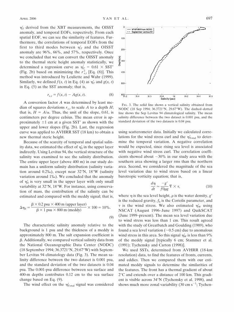
The characteristic salinity anomaly relative to thebackground is 1 psu and the thickness of a meddy isapproximately 800 m. The salt expansion coefficient is�. Additionally, we compared vertical salinity data fromthe National Oceanographic Data Center (NODC)(18 September 1994; 36.3721°N, 29.67°W) with Septem-ber Levitus 94 climatology data (Fig. 3). The mean sa-linity difference between the two dataset is 0.001 psu,and the standard deviation of the two datasets is 0.04psu. The 0.001-psu difference between sea surface and400-m depths contributes 0.12 cm to the sea surfacechange based on Eq. (9).

The wind effect on the ��Total signal was considered

using scatterometer data. Initially we calculated corre-lations for the wind stress curl and the ��Total to deter-mine the temporal variation. A negative correlationwould be expected, since rising sea level is associatedwith negative wind stress curl. The correlation coeffi-cients showed about �30% in our study area with thesouthern area showing a larger rms than the northernarea. Second, we considered the magnitude of the sealevel variation due to wind stress based on a linearbarotropic vorticity equation; that is,

d�

dt�

�g�

f 0g � �, �10�

where � is the sea level height, � is the water density, g�is the reduced gravity, f0 is the Coriolis parameter, and� is the wind stress. We also estimated ��W usingNSCAT (August 1996–June 1997) and QuikSCAT(June 1999–present). The mean sea level variation dueto wind stress was less than 1 cm. This result agreedwith the study of Greatbatch and Goulding (1989), whofound a sea level variation (0.5 cm) due to anomalouswind stress in this area. So this signal ��W is less than 9%of the meddy signal [typically 6 cm; Stammer et al.(1991); Tychensky and Carton (1998)].

We used SSTs, determined from AVHRR (18-kmresolution) data, to find the features of fronts, currents,and eddies. Then we compared them with our esti-mated meddy signals to determine the similarities ofthe features. The front has a thermal gradient of about2°C and extends over a distance of 100 km. This gradi-ent is visible across 34°N (Tychensky et al. 1998), andshows much more zonal variability (30 cm s�1; Tychen-

FIG. 3. The solid line shows a vertical salinity obtained fromNODC (18 Sep 1994; 36.3721°N, 29.67°W). The dashed–dottedline shows the Sep Levitus 94 climatological salinity. The meansalinity difference between the two dataset is 0.001 psu, and thestandard deviation of the two datasets is 0.04 psu.


sky et al. 1998) than is typically associated with meddytranslation [O(2–3 cm s �1)]. In addition, we comparedthe frontal features using a 15°C isothermal anomalydetermined by XBT measurements T�iso15°C, with boththe sea surface features illustrated by altimeter data��Total and the sea level variation ��T. The front featurescan be resolved by deriving thermal steric height andthus our new thermal steric height was derived from18-km-resolution AVHRR data, and was then removedfrom the altimetry for the O&M computation. Accord-ingly, by removing the thermal steric height variationdue to thermal variation and the front, this process (re-moval of ��T) could be used to enhance the meddy sig-nals at the isopycnal surface at the 400-m depth.

The mesoscale variability in the Azores–Madeura re-gion is dominated by the Azores Current and its asso-ciated eddies, which have dominant scales larger than300 km and 100 days (Le Traon and De Mey 1994). Thesurface eddies show larger diameters and shorter life-times than those of the meddies, and the surface eddiesare much faster than the meddies. The characteristictemporal and spatial features are different from meddysignals.

We also examined the Rossby wave in the map ofmeddy signals. It has been reported that the westward-propagating Rossby wave features and characteristicwavelength and frequencies are 2.7, 1.6, and 0.8km day�1 (Cipollini et al. 1997), and the period of thepeak energy is reduced crossing the ridge from 1 yr to7.9 months (Cromwell 2001). The two major peakscorrespond to components of wavelength 1440 and580 km, with periods of 330 and 220 days, respec-tively. Therefore, the characteristic temporal and spa-tial features are also different from meddy signals.

4. O&M signal and its validation

The result of �� Total � ��UL is apparently somevariation of the vertical water column, which is a con-sequence of the different incoming or outgoing watermasses under the upper layer. We can, therefore, inves-tigate the pathways of the O&M in the North Atlanticby using data with better spatial and temporal resolu-tion from space.

Data from the A Mediterranean Undercurrent Seed-ing Experiment (AMUSE; Bower et al. 1997) andStructures des Echanges Mer–Atmosphère, Propriétésdes Hétérogénéités Océaniques: Recherche Expéri-mentale (SEMAPHORE; Richardson and Tychensky1998) were used to confirm our estimation of the tra-jectories of the meddies and to study the variations ofthe meddies with time. The AMUSE data included an

observational component based on the successful seed-ing, on a weekly basis, of a total of 49 RAFOS floats inthe Mediterranean Undercurrent off southern Portu-gal, and 14 floats were embedded in meddies (Boweret al. 1997, their Table 2). The details of the data pro-cessing are described by Bower et al. (1997). TheSEMAPHORE experiments using RAFOS floatsshowed 10 floats embedded in meddies (Richardsonand Tychensky 1998, their Table 1). The details of thedata processing for these experiments are described byRichardson and Tychensky (1998). During AMUSE,nine floats registered six meddy formation events in thevicinity of Cape St. Vincent and three at the Estrema-dura Promontory (Bower et al. 1997). Furthermore, sixother floats revealed the presence of meddies as theywere caught in the periphery of these structures.

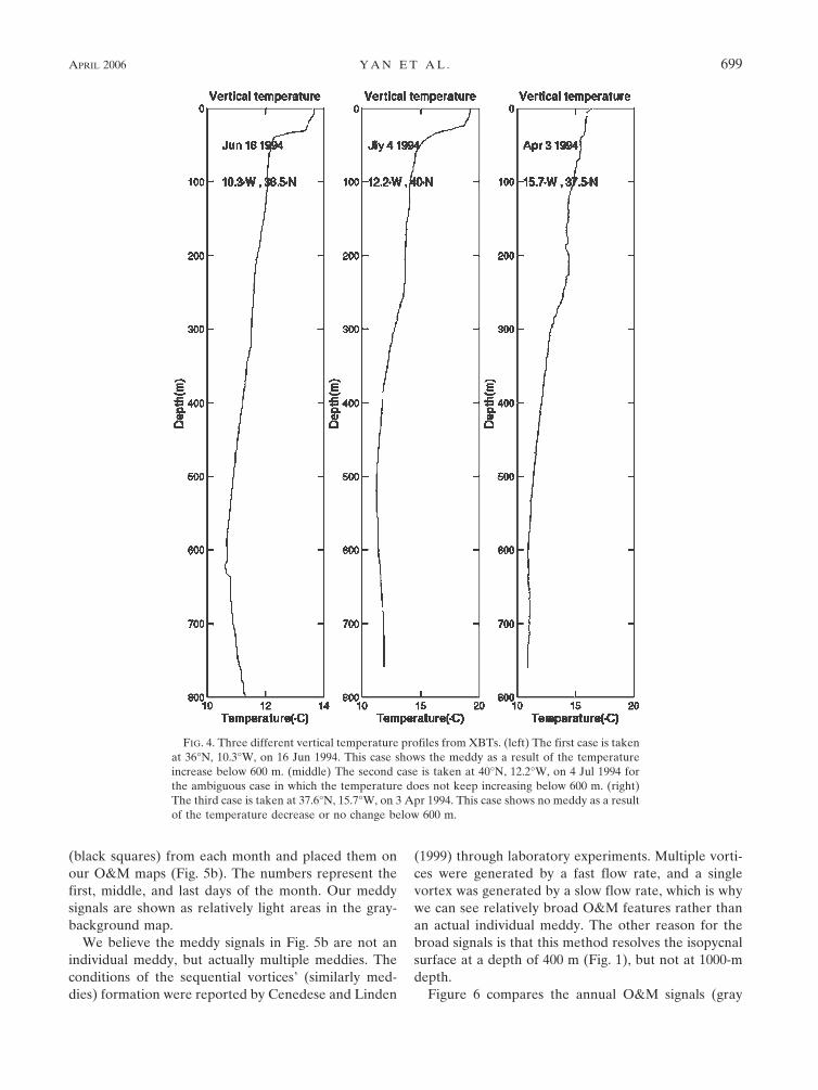
For more validation of the meddies’ location, the ver-tical temperature distribution measured at depths thatreached 700 m was used. The individual XBT data wereobtained from the NODC in the Global Temperature–Salinity Profile Program database (more informationavailable online at http://www.nodc.noaa.gov/GTSPP/gtspp-bc.html). Out of the 298 XBT measurements inour study area during 1994, 121 measurements showedthat the maximum depth of 700 m was exceeded. These121 measurements were examined for meddy locations.Figure 4 shows the three different cases used to deter-mine whether there was a meddy or not below 700-mdepths. The first case (left panel in Fig. 4) implies thata meddy exists at depth (11 measurements found) de-termined by when the temperature difference of thedeepest 100-m interval increases by 0.5°C or more, thesecond case (right panel in Fig. 4) implies that a meddydoes not exist at depth (55 measurements found) whenthe temperature difference of the deepest 100-m inter-val decreases by 0.5°C or less, and the third case(middle panel in Fig. 4) implies an ambiguous case be-cause of negligible temperature change (55 measure-ments found). Accordingly, the data from the first casewere compared with meddy features determined by ourmethod and by float observations in 1994. In fact, manystudies showed the vertical temperature associated withthe presence of a meddy (Tychensky and Carton 1998,their Plate 5; Richardson and Tychensky 1998, theirFig. 3; Schultz Tokos and Rossby 1991, their Fig. 2;Richardson et al. 1989, their Fig. 1).

To make comparisons in time between a real floattrajectory, AM129, and our O&M signals, the trajec-tory of the AM129 is introduced in Fig. 5a. We can seean anticyclonic feature from the middle of March toSeptember 1994. For more details on the meddy floats,one can refer to Bower et al.’s (1997) Table 2. For aspecific comparison, we chose three points for floats


(black squares) from each month and placed them onour O&M maps (Fig. 5b). The numbers represent thefirst, middle, and last days of the month. Our meddysignals are shown as relatively light areas in the gray-background map.

We believe the meddy signals in Fig. 5b are not anindividual meddy, but actually multiple meddies. Theconditions of the sequential vortices’ (similarly med-dies) formation were reported by Cenedese and Linden

(1999) through laboratory experiments. Multiple vorti-ces were generated by a fast flow rate, and a singlevortex was generated by a slow flow rate, which is whywe can see relatively broad O&M features rather thanan actual individual meddy. The other reason for thebroad signals is that this method resolves the isopycnalsurface at a depth of 400 m (Fig. 1), but not at 1000-mdepth.

Figure 6 compares the annual O&M signals (gray

FIG. 4. Three different vertical temperature profiles from XBTs. (left) The first case is takenat 36°N, 10.3°W, on 16 Jun 1994. This case shows the meddy as a result of the temperatureincrease below 600 m. (middle) The second case is taken at 40°N, 12.2°W, on 4 Jul 1994 forthe ambiguous case in which the temperature does not keep increasing below 600 m. (right)The third case is taken at 37.6°N, 15.7°W, on 3 Apr 1994. This case shows no meddy as a resultof the temperature decrease or no change below 600 m.


map) with floats (black circles and diamonds). Most offloats are related to our high O&M signal. If we allowed2–3-cm uncertainties on the meddy signals, then 72%(2 cm)–64% (3 cm) of the float observations agreed

with our results. It should be pointed out that in somelocations in Fig. 6, for example, 35°N and 18°W in 1994,there are no black solid circles to compare or matchwith the meddy signal from our method. We believe

FIG. 5. (a) The trajectory of float AM129 from March to September 1994. Thearrows indicate the first day of each month. The bathymetry is shown with differentline styles [labeled at �1000- (dashed–dotted), �2000- (dotted), and �3000-m(solid) depths]. (b) The locations of float AM129 are overlain on a grayscale O&Mmap. The numbers (1, 2, and 3) represent the first, middle, and last day of eachmonth, respectively.


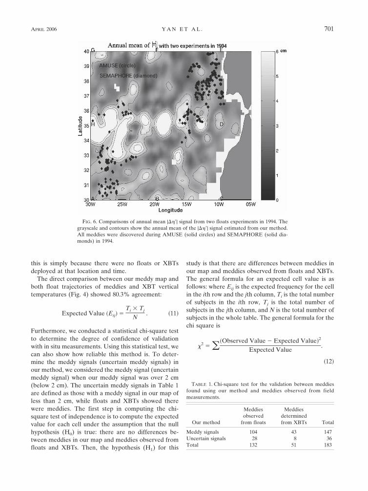
this is simply because there were no floats or XBTsdeployed at that location and time.

The direct comparison between our meddy map andboth float trajectories of meddies and XBT verticaltemperatures (Fig. 4) showed 80.3% agreement:

Expected Value �Eij� �Ti � Tj

N. �11�

Furthermore, we conducted a statistical chi-square testto determine the degree of confidence of validationwith in situ measurements. Using this statistical test, wecan also show how reliable this method is. To deter-mine the meddy signals (uncertain meddy signals) inour method, we considered the meddy signal (uncertainmeddy signal) when our meddy signal was over 2 cm(below 2 cm). The uncertain meddy signals in Table 1are defined as those with a meddy signal in our map ofless than 2 cm, while floats and XBTs showed therewere meddies. The first step in computing the chi-square test of independence is to compute the expectedvalue for each cell under the assumption that the nullhypothesis (H0) is true: there are no differences be-tween meddies in our map and meddies observed fromfloats and XBTs. Then, the hypothesis (H1) for this

study is that there are differences between meddies inour map and meddies observed from floats and XBTs.The general formula for an expected cell value is asfollows: where Eij is the expected frequency for the cellin the ith row and the jth column, Ti is the total numberof subjects in the ith row, Tj is the total number ofsubjects in the jth column, and N is the total number ofsubjects in the whole table. The general formula for thechi square is

�2 � �Observed Value � Expected Value�2

Expected Value.

�12�

TABLE 1. Chi-square test for the validation between meddiesfound using our method and meddies observed from fieldmeasurements.

Our method

Meddiesobserved

from floats

Meddiesdeterminedfrom XBTs Total

Meddy signals 104 43 147Uncertain signals 28 8 36Total 132 51 183

FIG. 6. Comparisons of annual mean |��| signal from two floats experiments in 1994. Thegrayscale and contours show the annual mean of the |��| signal estimated from our method.All meddies were discovered during AMUSE (solid circles) and SEMAPHORE (solid dia-monds) in 1994.


The number of degrees of freedom (df) is 1: df � n �1, where n is the number of classes. The obtained totalprobability (P value) is 0.6 for Table 1. In our chi-square test, the 0.05 probability level as our criticalvalue corresponds to a 3.1 P value. Because the calcu-lated chi-square value (or P value) is less than the criti-

cal value in the 95% significant level, we reject thehypothesis. Therefore, we accept the null hypothesis:there are no differences between meddies in ourmethod and meddies observed from field observations.

Results from our method are classified into two cat-egories based on the criterion of the 2-cm signal of the

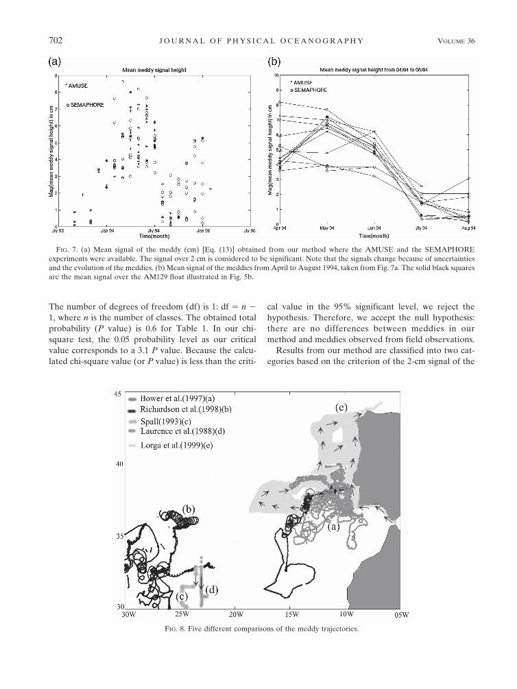
FIG. 7. (a) Mean signal of the meddy (cm) [Eq. (13)] obtained from our method where the AMUSE and the SEMAPHOREexperiments were available. The signal over 2 cm is considered to be significant. Note that the signals change because of uncertaintiesand the evolution of the meddies. (b) Mean signal of the meddies from April to August 1994, taken from Fig. 7a. The solid black squaresare the mean signal over the AM129 float illustrated in Fig. 5b.

FIG. 8. Five different comparisons of the meddy trajectories.


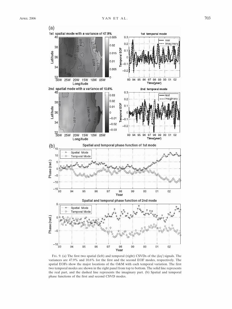
FIG. 9. (a) The first two spatial (left) and temporal (right) CSVDs of the |��| signals. Thevariances are 47.9% and 10.6% for the first and the second EOF modes, respectively. Thespatial EOFs show the major locations of the O&M with each temporal variation. The firsttwo temporal modes are shown in the right panel from top to bottom. The solid line representsthe real part, and the dashed line represents the imaginary part. (b) Spatial and temporalphase functions of the first and second CSVD modes.


meddies: one is for the meddy signals (signals � 2 cm)validated by floats and XBTs (second row in Table 1),and the other is for the uncertain signals of our method(signals � 2 cm) while floats and XBTs showed therewere meddies (third row in Table 1) determined bycomparing our estimated O&M signals with floats andXBTs. From Table 1, the percentages of the significantmeddy signals and uncertain meddy signals in ourmethod are 80.3% (�147/183 � 100) and 19.7% (�36/183 � 100), respectively.

5. Analysis results

The annual comparison between field observationsand our computation was very good and is shown in Fig.6. In addition, Fig. 7a shows the monthly mean meddysignals, which were obtained for every float in eachmonth (t � 1–n days). Therefore, we can estimate therelative magnitude of the O&M at the same place as thefloat trajectories in given months. This magnitude(Mag) was computed using the monthly mean meddysignals from our method for each float during eachmonth; that is,

Mab � l�1

n

��T, S, W, X, t� l, (13)

where l represents the locations of the floats. The meanranges were within 0–9 cm. We can see the time seriesof the meddy signal as being on the order of 5 cm.Stammer et al. (1991) and Tychensky and Carton(1998) showed a similar order of magnitude (6 cm).To demonstrate the variation of the O&M signals dur-ing specific periods, we plotted the mean O&M [Eq.(13)] from April to August 1994 in Fig. 7b. The blacksquare represents the monthly mean magnitude of ourmeddy signals at the same place as the AM129 trajec-tories in given months as illustrated in Figs. 5a and 5b.The monthly mean meddy signals are 3.8, 7.4, 5, and 1.5cm, from April to July, respectively. Each float has adifferent formation date and lifetime, but generallythey are slowly decaying during these periods.

A comparison was also made with five studies, shownin Fig. 8. Bower et al. (1997) conducted experimentsbetween May 1993 and March 1994, where 49 RAFOSfloats were deployed in the Mediterranean Undercur-rent off southern Portugal. These floats were acousti-cally tracked for up to 11 months and nine meddy for-mation events were observed: six near Cape St. Vin-cent, and three near the Estremadura Promontoryalong the western Portuguese continental slope. Ameddy formation rate of 15–20 meddies per year wasestimated. Richardson et al. (1989) estimated 8–12

meddies. The AMUSE meddies dispersed over the re-gion between 33° and 42°N and between 7° and 17°W.Richardson and Tychensky (1998) obtained 10 meddyobservations during the SEMAPHORE experiment.Spall et al. (1993) used SOFAR floats and observed aspecific meddy in October 1984. Armi et al. (1989)showed Lagrangian trajectories from SOFAR floats,which were launched at 32°N, 24°W between 1984 and1988. Iorga and Lozier (1999) used around 14 000 hy-drographic stations in the North Atlantic, spanning theperiod 1904–90. They produced diagnostic modes in theeastern basin. Our study confirmed all the trajectoriesreported by the second and the third investigators. Forthe other studies, we could not make comparisons be-cause there were no altimeter data available. As seen inthe other studies, westward and southward meddieswere observed in areas similar to those investigatedduring the period 1993–2002.

To study major spatial patterns of the O&M, we ap-plied CSVD (Fig. 9a). The first two spatial EOFs ac-count for 47.9% and 10.6% of the total variance, re-spectively. The high variation occurs in the major re-gions of the Mediterranean outflow, and the meddies’formation sites. The regions of small variation repre-sent standing but oscillating features. The second spa-tial EOF shows high variation across 25°W, which hasthe inverse phase of Mediterranean outflow in the Gulfof Cadiz. The right panel of Fig. 9 shows the first andsecond temporal EOFs for a real part (solid line) andfor an imaginary part (dashed line), respectively. Thefirst spatial EOF shows a possible main trajectory of theO&M with annual signals with a maximum in borealautumn and a minimum in boreal spring from the real

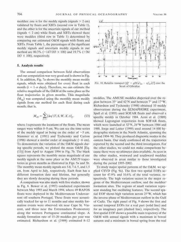
FIG. 10. Relative transport [Q� � gD(��|x2 � ��|x1)/f ] over theStrait of Gibraltar.


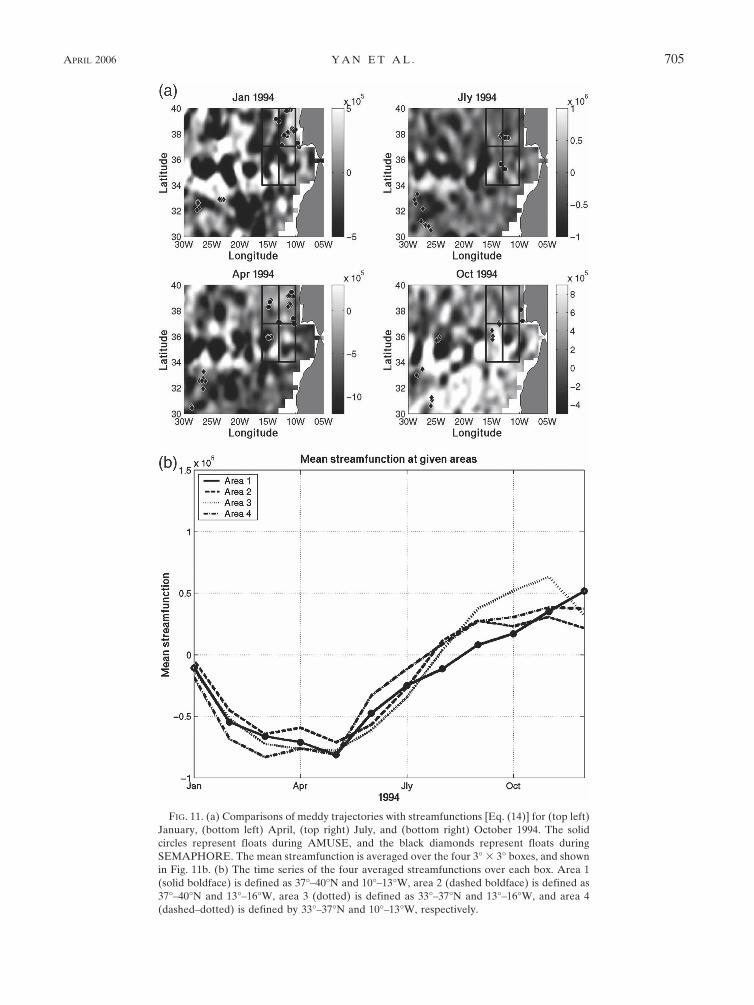
FIG. 11. (a) Comparisons of meddy trajectories with streamfunctions [Eq. (14)] for (top left)January, (bottom left) April, (top right) July, and (bottom right) October 1994. The solidcircles represent floats during AMUSE, and the black diamonds represent floats duringSEMAPHORE. The mean streamfunction is averaged over the four 3° � 3° boxes, and shownin Fig. 11b. (b) The time series of the four averaged streamfunctions over each box. Area 1(solid boldface) is defined as 37°–40°N and 10°–13°W, area 2 (dashed boldface) is defined as37°–40°N and 13°–16°W, area 3 (dotted) is defined as 33°–37°N and 13°–16°W, and area 4(dashed–dotted) is defined by 33°–37°N and 10°–13°W, respectively.


part. Meanwhile, the phase changes with a maximum inboreal spring and a minimum in boreal autumn. Whena maximum changes to a minimum, the spatial featuresare reversed, or vice versa.

Using Eq. (6) we computed the spatial and temporalfunction variations in terms of a wavenumber k andangular velocity � (Fig. 9b). As Susanto et al. (1998)

demonstrated, the slope of the spatial function repre-sents the wavenumber, and the slope of the temporalfunction represents the angular frequency. We coulddetermine slopes after 2000 for the first spatial and tem-poral function as 0.4 and �0.4, respectively. Thus, thefirst CSVD shows the westward phase speed (c � �/k),�1 cm s�1. Likewise, the second CSVD shows the

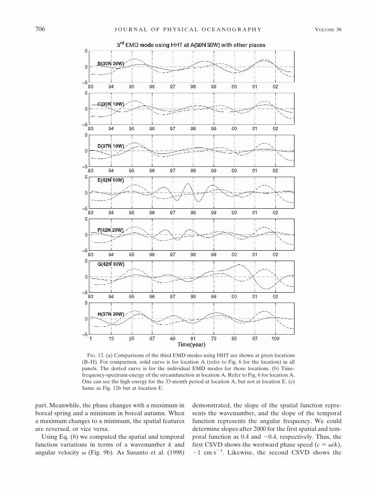
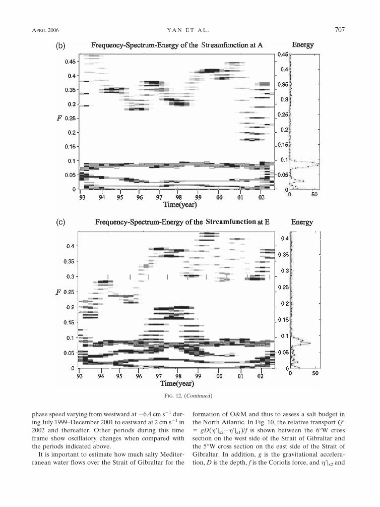
FIG. 12. (a) Comparisons of the third EMD modes using HHT are shown at given locations(B–H). For comparison, solid curve is for location A (refer to Fig. 6 for the location) in allpanels. The dotted curve is for the individual EMD modes for those locations. (b) Time-frequency-spectrum-energy of the streamfunction at location A. Refer to Fig. 6 for location A.One can see the high energy for the 33-month period at location A, but not at location E. (c)Same as Fig. 12b but at location E.


phase speed varying from westward at �6.4 cm s�1 dur-ing July 1999–December 2001 to eastward at 2 cm s�1 in2002 and thereafter. Other periods during this timeframe show oscillatory changes when compared withthe periods indicated above.

It is important to estimate how much salty Mediter-ranean water flows over the Strait of Gibraltar for the

formation of O&M and thus to assess a salt budget inthe North Atlantic. In Fig. 10, the relative transport Q�� gD(��|x2��|x1)/f is shown between the 6°W crosssection on the west side of the Strait of Gibraltar andthe 5°W cross section on the east side of the Strait ofGibraltar. In addition, g is the gravitational accelera-tion, D is the depth, f is the Coriolis force, and ��|x2 and

FIG. 12. (Continued)


��|x1 are the sea level variations at places x2 and x1,respectively. Because the exact thickness of the O&Mcannot be estimated, we computed Q�/D with respect totime. We can interpret Fig. 10 as follows: if there ismore salty Mediterranean water over the Strait ofGibraltar, the salt steric height decreases, which thusdecreases the total sea surface height. The Mediterra-nean water, which can be dense because of evaporationin the eastern basin, flows westward below the surfacealong the western Mediterranean Sea and out throughthe Strait of Gibraltar into the Atlantic. The oppositeholds for the positive relative anomaly during winter-time.

To investigate the reasons for the change in the di-rection of propagation of meddies with respect to seasurface variation, the streamfunction � was computedusing the altimetry. This representation of the stream-function allows observations of the interactions be-tween the sea surface gradient and the meddies’ propa-gation. The computation of the sea surface heightanomaly �� in terms of the usual dynamic variables isstraightforward if the flow is assumed to be quasigeo-strophic: the streamfunction � is defined as

� �g

f0��Total, �14�

where � is the surface quasigeostrophic streamfunction(e.g., Douglas et al. 1983).

This is illustrated to examine the seasonal migrationof the tropical water moving toward the north and polarwater moving toward south over the O&M signals (Fig.11a). Because most of meddies are generated nearCape St. Vincent at the southwestern corner of the Ibe-rian Penisula, we made four 3° � 3° boxes along 37°Nto understand the response of the O&M due to changesof sea surface pressure gradients (Fig. 11a). Figure 11bshows the time series of the averaged streamfunctionover each box. From January to May 1994, high seasurface height in area 2 produces a pressure gradienttoward area 4. Similarly, from May to August, there isa pressure gradient from area 4 to area 3; from Augustto November, there is a pressure gradient from area 3to area 1, respectively. We compared the meddies mea-sured by the floats and the streamfunctions in all themonths in the experimental periods and found that themeddies preferred to travel toward the low streamlinesand stayed within the northernmost and southernmoststreamlines in April and October, respectively.

To find out the dominant signal of the sea surfaceinteraction with the meddies, the HHT was applied totheir EMD modes. We chose eight places to investigatethe dominant signal in our study area. Figure 12a showsthat place groups 1 (B, C, and D, shown in Fig. 6) and

2 (H and G, shown in Fig. 6) have similar signals. How-ever, group 3 (E and F, shown in Fig. 6) has a slightlydifferent signal from groups 1 and 2. Consequently,there were seasonal fluctuations between location Aand group 3. To compute the dominant signal of thepower for locations A and E, the HHT was employedand is shown in Figs. 12b and 12c. In both, the dominantfrequency F was around F � 0.082 (1 yr). However,location A had a lower frequency, 0.03 (33.3 months),which seems to indicate that wind stress with 33.3-month period produces sea surface forcing. The surfacevariations produce the baroclinic instability on themeddies, which is related to southward translation. Thesouthward translation of the meddies due to the baro-clinic effects was consistent with that discussed byMüler and Siedler (1992) and by Käse and Zenk (1996).If the current is vertically sheared in a stratified fluid,baroclinic instability can occur.

6. Conclusions

In analyzing the trajectories of O&M, sea surfaceheight anomalies were calculated and examined usingsatellite altimetry, IR satellite imagery, XBT tempera-ture fields, and scatterometer wind measurements. Sat-ellite observations provided a good way to overcomethe limitations of the spatial and temporal coverage offield measurements. Using spaceborne measurements,we have shown the spatial and temporal variations ofthe O&M trajectories in the North Atlantic Ocean. Thevalidations were conducted using data from theAMUSE and the SEMAPHORE experiments andXBT measurements for the vertical temperature distri-bution. Most of the floats and XBTs’ meddy cases werelocated in the high signal areas of the O&M map weproduced.

We also calculated the relative transport of saltyMediterranean water over the Strait of Gibraltar. Wefound that saltier water from the Mediterranean Seawas transported into the North Atlantic in boreal springand summer relative to boreal autumn and winter. Themeddies’ propagating directions were related to seasurface geostrophic flow, and the meddies were con-fined within the north and south boundaries, which re-vealed seasonal variability. Meddies tended to traveltoward low streamlines, because of the pressure of thesurface pushing the meddies toward the low pressureareas. Interpolation and wind stress errors could causepossible error in this study, but they were not significantin comparison with the real signals. We believe that thisis an improved effort (studying a very interesting phe-nomenon at the 400-m-depth isopycnal surface fromspace) that has been achieved successfully using state-of-the-art satellite multisensor remote sensing data.


Acknowledgments. We thank R. W. Garvine forproofreading the manuscript and providing comments,and C. Wunsch for reading an earlier version of themanuscript and giving helpful comments and sugges-tions on that version. We also thank the SIO/JEDACenter for providing the heat storage data, A. Bower,and P. Richardson for providing floats data at theWHOI Float Operations Group. This research was sup-ported partially by the National Aeronautics and SpaceAdministration (NASA) through Grant NAG5-12745,by the Office of Naval Research (ONR) through GrantN00014-03-1-0337, and by the National Oceanic andAtmospheric Administration (NOAA) through GrantNA17EC2449. Author W. T. Liu is supported by theNASA Physical Oceanography Program. We alsothank the anonymous reviewers for their valuable com-ments and encouragement.

REFERENCES

Armi, L., and H. Stommel, 1983: Four views of a portion of theNorth Atlantic subtropical gyre. J. Phys. Oceanogr., 13, 828–857.

——, and W. Zenk, 1984: Large lenses of highly saline Mediter-ranean salt lens. J. Phys. Oceanogr., 14, 1560–1576.

——, D. Hebert, N. Oakey, J. Price, P. Richardson, T. Rossby, andB. Ruddick, 1989: Two years in the life of a Mediterraneansalt lens. J. Phys. Oceanogr., 19, 354–370.

Barnett, T. P., 1983: Interaction of the monsoon and Pacific tradewind systems at interannual time scales. Part I: The equato-rial zone. Mon. Wea. Rev., 111, 756–773.

Bower, A. S., L. Armi, and I. Ambar, 1997: Lagrangian observa-tions of eddy formation during A Mediterranean Undercur-rent Seeding Experiment. J. Phys. Oceanogr., 27, 2545–2575.

Bretherton, C. S., C. Smith, and J. M. Wallace, 1992: An inter-comparison of methods for finding coupled patterns in cli-mate data. J. Climate, 5, 541–560.

Cenedese, C., and P. F. Linden, 1999: Cyclone and anticycloneformation in a rotating stratified fluid over a sloping bottom.J. Fluid Mech., 381, 199–223.

Cipollini, P., D. Cromwell, M. S. Jones, G. D. Quartly, and P. G.Challenor, 1997: Concurrent altimeter and infrared observa-tions of Rossby wave propagation near 34°N in the northeastAtlantic. Geophys. Res. Lett., 24, 889–892.

Cromwell, D., 2001: Sea surface height observations of the 34°N“waveguide” in the North Atlantic. Geophys. Res. Lett., 28,3705–3708.

Douglas, B. C., R. E. Cheney, and R. W. Agreen, 1983: Eddy en-ergy of the northwest Atlantic and Gulf of Mexico deter-mined from GEOS 3 altimetry. J. Geophys. Res., 88, 9595–9603.

Greatbatch, R., and A. Goulding, 1989: Seasonal variations in alinear barotropic model of the North Atlantic driven by theHellerman and Rosenstein wind stress field. J. Phys. Ocean-ogr., 19, 572–595.

Huang, N., and Coauthors, 1998: The empirical mode decompo-sition and Hilbert spectrum for nonlinear and nonstationarytime series analysis. Proc. Roy. Soc. Math., Phys. Eng. Sci.,454, 903–995.

Iorga, M. C., and M. S. Lozier, 1999: Signature of the Mediterra-nean outflow from a North Atlantic climatology, 1. Salinityand density fields. J. Geophys. Res., 104, 25 985–26 009.

Käse, R. H., and W. Zenk, 1987: Reconstructed Mediterraneansalt lens trajectories. J. Phys. Oceanogr., 17, 158–163.

——, and ——, 1996: Structure of the Mediterranean Water andmeddy characteristics in the northeastern Atlantic. OceanCirculation and Climate (Observation and Modeling theGlobal Ocean), W. Krauss, Ed., Gebr. Borntraeger, 365–395.

Le Traon, P. Y., and P. De Mey, 1994: The eddy field associatedwith the Azores Front east of the Mid-Atlantic Ridge as ob-served by the Geosat altimeter. J. Geophys. Res., 99, 9907–9923.

Leuliette, E. W., and J. M. Wahr, 1999: Coupled pattern analysisof sea surface temperature and TOPEX/Poseidon sea surfaceheight. J. Phys. Oceanor., 29, 599–611.

Levitus, S., and T. P. Boyer, 1994: Temperature. Vol. 4, WorldOcean Atlas, NOAA Atlas NESDIS 4, 117 pp.

McDowell, S., and H. Rossby, 1978: Mediterranean Water: Anintense mesoscale eddy off the Bahamas. Science, 202, 1085–1087.

Müler, T. J., and G. Siedler, 1992: Multi-year current time series inthe eastern North Atlantic Ocean. J. Mar. Res., 50, 63–98.

Oliveira, P. B., A. Nuno Serra, F. G. Fiuza, and I. Ambar, 2000: Astudy of meddies using simultaneous in-situ and satellite ob-servations. Satellites, Oceanography and Society, D. Halpern,Ed., Elsevier Oceaongraphy Series, Elsevier, 125–148.

Peng, S., and J. Fyfe, 1996: The coupled pattern between sea levelpressure and sea surface temperature in the midlatitudeNorth Atlantic. J. Climate, 9, 1824–1839.

Pingree, R., and B. Le Cann, 1992: Three anticyclonic slope wateroceanic eddies (SWODDIES) in the southern Bay of Biscayin 1990. Deep-Sea Res., 39, 1147–1175.

——, and ——, 1993: A shallow meddy (a smeddy) from thesecondary Mediterranean salinity maximum. J. Geophys.Res., 98, 20 169–20 185.

Reynolds, R. W., and T. M. Smith, 1994: Improved global sea sur-face temperature analyses using optimum interpolation. J.Climate, 7, 929–948.

Richardson, P. L., and A. Tychensky, 1998: Meddy trajectories inthe Canary Basin measured during the SEMAPHORE ex-periment, 1993–1995. J. Geophys. Res., 103, 25 029–25 045.

——, D. Walsh, L. Armi, M. Schröder, and J. F. Price, 1989:Tracking three meddies with SOFAR floats. J. Phys. Ocean-ogr., 19, 371–383.

——, A. S. Bower, and W. Zenk, 2000: A census of meddiestracked by fronts. Progress in Oceanography, Vol. 45, Perga-mon, 209–250.

Schultz Tokos, K. L., and T. Rossby, 1991: Kinematics and dy-namics of a Mediterranean salt lens. J. Phys. Oceanogr., 21,879–892.

Spall, M. A., P. L. Richardson, and J. Price, 1993: Advection andeddy mixing in the Mediterranean salt tongue. J. Mar. Res.,51, 797–818.

Stammer, D., H. H. Hinrichsen, and R. H. Käse, 1991: Can med-dies be detected by satellite altimetry? J. Geophys. Res., 96,7005–7014.

Susanto, R. D., Q. Zheng, and X.-H. Yan, 1998: Complex singularvalue decomposition analysis of equatorial waves in the Pa-cific observed by TOPEX/Poseidon altimeter. J. Atmos. Oce-anic Technol., 15, 764–774.

Tokmakian, R. T., and P. G. Challenor, 1993: Observations in the


Canary Basin and the Azores frontal region using Geosatdata. J. Geophys. Res., 98, 4761–4773.

Tychensky, A., and X. Carton, 1998: Hydrological and dynamicalcharacterization of meddies in the Azores region: A para-digm for baroclinic vortex dynamics. J. Geophys. Res., 103,25 061–25 079.

——, P.-Y. Le Traon, F. Hernanez, and D. Jourdan, 1998: Largestructures and temporal change in the Azores front duringthe SEMAPHORE experiment. J. Geophys. Res., 103,25 009–25 027.

Wallace, J. M., C. Smith, and C. S. Bretherton, 1992: Singularvalue decomposition of wintertime sea surface temperatureand 500-mb height anomalies. J. Climate, 5, 561–576.

Wilson, W., and D. Bradley, 1966: Specific volume, thermal ex-

pansion and isothermal compressibility of seawater. U.S. Na-val Ordnance Laboratory Tech. Rep. 66-103.

Yan, X.-H., and A. Okubo, 1992: Three-dimensional analyticalmodel for the mixed layer depth. J. Geophys. Res., 97, 20 201–20 226.

——, J. R. Schubel, and D. W. Pritchard, 1990: Oceanic uppermixed layer depth determination by the use of satellite data.Remote Sens. Environ., 32, 55–74.

——, A. Okubo, J. R. Shubel, and D. W. Pritchard, 1991a: Ananalytical mixed layer remote sensing model. Deep-Sea Res.,38, 267–287.

——, P. P. Niller, and R. H. Stewart, 1991b: Construction andaccuracy analysis of images of the daily-mean mixed layerdepth. Int. J. Remote Sens., 12, 2573–2584.


A New Study of the Mediterranean Outflow, Air Sea Interactions, and Meddies Using Multisensor Data

Documents

Transcript of A New Study of the Mediterranean Outflow, Air Sea Interactions, and Meddies Using Multisensor Data