A New Statistic for Influence in Linear Regression
12
A New Statistic for Influence in Linear Regression Daniel PEÑA Department of Statistics Universidad Carlos III de Madrid 28907 Getafe, Madrid, Spain ([email protected]) Since the seminal article by Cook, the usual way to measure the influence of an observation in a statistical model is to delete the observation from the sample and compute a convenient norm of the change in the parameters or in the vector of forecasts. In this article we define a new way to measure the influence of an observation based on how this observation is being influenced by the rest of the data. More precisely, the new statistic we propose is defined as the squared norm of the vector of changes of the forecast of one observation when each of the sample points are deleted one by one. We prove that this new statistic has asymptotically a normal distribution and is able to detect a group of high leverage similar outliers that will be undetected by Cook’s statistic. We show in several examples that the proposed statistic is useful for detecting heterogeneity in regression models in large high-dimensional datasets. KEY WORDS: Cook’s distance; Influential observation; Large dataset; Leverage; Masking; Outlier. 1. INTRODUCTION The seminal article by Cook (1977) had a strong influence on the study of outliers and model diagnostics. The books of Belsley, Kuh, and Welsch (1980), Cook and Weisberg (1982), Atkinson (1985), and Chatterjee and Hadi (1988) surveyed the field with applications to linear regression and other models. The study of influential observations has been extended to other statistical models using similar ideas to the ones developed in linear regression. (See Pregibon 1981 for logistic regression models, Williams 1987 for generalized linear models, and Peña 1990 for time series models.) Influence is usually defined by modifying the weights at- tached to a point or group of points in the sample and look- ing at the standardized change of the parameter vector or the vector of forecasts. The point can be deleted, as proposed by Cook (1977) and Belsley at al. (1980), or its weight can be de- creased, as in the local influence analysis introduced by Cook (1986). The local influence approach can also be used to intro- duce perturbations in specific directions of interest in a sam- ple. (See Brown and Lawrence 2000 and Suárez Rancel and González Sierra 2001 for reviews of local influence in regres- sion and many references, and Hartless, Booth, and Littell 2003 for recent results on this approach.) A related way to analyze in- fluence by an extension of the influence curve methodology has been proposed by Critchley, Atkinson, Lu, and Biazi (2001). In this article we introduce a new way to analyze influence. Instead of looking at how the deletion of a point or the introduc- tion of same perturbation affects the parameters, the forecasts, or the likelihood function, we look at how each point is influ- enced by the others in the sample. That is, for each sample point we measure the forecasted change when each other point in the sample is deleted. In this way we measure the sensitivity of each case to changes in the entire sample. We show that this type of influence analysis complements the usual one and is able to indicate features in the data, such as clusters of high-leverage outliers, that are very difficult to detect by the usual influence statistics. For instance, it is well known that univariate influen- tial statistics fail when we have a group of high-leverage outliers (see, e.g., Lawrance 1995 for a detailed analysis and Rousseeuw and Leroy 1987 for several examples). We show that the pro- posed statistic will indicate this type of situation. This statis- tic complements the usual influence analysis, and, in particular, a plot of a standard influence statistic, such as Cook’s distance, and the proposed sensitivity statistic can be a useful diagnos- tic tool in linear regression. The proposed statistic can also be used together with any modification of Cook’s distance, such as those proposed by Belsley et al. (1980), Atkinson (1981), and Welsch (1982), among others. (See Cook, Peña, and Weisberg 1988 for a comparison of some of these modifications.) The objective of this article is not to propose a procedure for unmasking outliers or robust regression. Many procedures have been developed to solve these problems. (See, e.g., Rousseeuw 1984, Atkinson 1994, and Peña and Yohai 1999 and the refer- ences therein for outlier detection based on robust estimation, and Justel and Peña 2001 for a Bayesian approach to these prob- lems.) We do not claim that the simple statistic that we propose will always be able to avoid masking; we do not suggest that this statistic can provide the same information as some of the computationally intensive methods. Our objective here is rather to propose a new statistic, very simple to compute and with an intuitive interpretation, that can be a useful tool in applied re- gression analysis. In particular, it can be very effective in large datasets in high dimension, where more sophisticated proce- dures are difficult to apply because of their high computational requirements. The article is organized as follows. In the next section we present the notation and define our proposed statistic. In Sec- tion 3 we analyze some of its properties. In Section 4 we il- lustrate the application of this statistic in four examples, and in Section 5 we discuss the relationship between the proposed statistic and other procedures. Finally, in Section 6 we comment on the generalization of the proposed statistic to other statistical models. © 2005 American Statistical Association and the American Society for Quality TECHNOMETRICS, FEBRUARY 2005, VOL. 47, NO. 1 DOI 10.1198/004017004000000662 1
-
Upload
independent -
Category
Documents
-
view
0 -
download
0
Transcript of A New Statistic for Influence in Linear Regression

A New Statistic for Influence inLinear Regression
Daniel PENtildeA
Department of StatisticsUniversidad Carlos III de Madrid
28907 Getafe Madrid Spain(danielpenauc3mes)
Since the seminal article by Cook the usual way to measure the influence of an observation in a statisticalmodel is to delete the observation from the sample and compute a convenient norm of the change in theparameters or in the vector of forecasts In this article we define a new way to measure the influence ofan observation based on how this observation is being influenced by the rest of the data More preciselythe new statistic we propose is defined as the squared norm of the vector of changes of the forecast ofone observation when each of the sample points are deleted one by one We prove that this new statistichas asymptotically a normal distribution and is able to detect a group of high leverage similar outliers thatwill be undetected by Cookrsquos statistic We show in several examples that the proposed statistic is usefulfor detecting heterogeneity in regression models in large high-dimensional datasets
KEY WORDS Cookrsquos distance Influential observation Large dataset Leverage Masking Outlier
1 INTRODUCTION
The seminal article by Cook (1977) had a strong influenceon the study of outliers and model diagnostics The books ofBelsley Kuh and Welsch (1980) Cook and Weisberg (1982)Atkinson (1985) and Chatterjee and Hadi (1988) surveyed thefield with applications to linear regression and other modelsThe study of influential observations has been extended to otherstatistical models using similar ideas to the ones developed inlinear regression (See Pregibon 1981 for logistic regressionmodels Williams 1987 for generalized linear models and Pentildea1990 for time series models)
Influence is usually defined by modifying the weights at-tached to a point or group of points in the sample and look-ing at the standardized change of the parameter vector or thevector of forecasts The point can be deleted as proposed byCook (1977) and Belsley at al (1980) or its weight can be de-creased as in the local influence analysis introduced by Cook(1986) The local influence approach can also be used to intro-duce perturbations in specific directions of interest in a sam-ple (See Brown and Lawrence 2000 and Suaacuterez Rancel andGonzaacutelez Sierra 2001 for reviews of local influence in regres-sion and many references and Hartless Booth and Littell 2003for recent results on this approach) A related way to analyze in-fluence by an extension of the influence curve methodology hasbeen proposed by Critchley Atkinson Lu and Biazi (2001)
In this article we introduce a new way to analyze influenceInstead of looking at how the deletion of a point or the introduc-tion of same perturbation affects the parameters the forecastsor the likelihood function we look at how each point is influ-enced by the others in the sample That is for each sample pointwe measure the forecasted change when each other point in thesample is deleted In this way we measure the sensitivity of eachcase to changes in the entire sample We show that this typeof influence analysis complements the usual one and is able toindicate features in the data such as clusters of high-leverageoutliers that are very difficult to detect by the usual influencestatistics For instance it is well known that univariate influen-tial statistics fail when we have a group of high-leverage outliers
(see eg Lawrance 1995 for a detailed analysis and Rousseeuwand Leroy 1987 for several examples) We show that the pro-posed statistic will indicate this type of situation This statis-tic complements the usual influence analysis and in particulara plot of a standard influence statistic such as Cookrsquos distanceand the proposed sensitivity statistic can be a useful diagnos-tic tool in linear regression The proposed statistic can also beused together with any modification of Cookrsquos distance such asthose proposed by Belsley et al (1980) Atkinson (1981) andWelsch (1982) among others (See Cook Pentildea and Weisberg1988 for a comparison of some of these modifications)
The objective of this article is not to propose a procedure forunmasking outliers or robust regression Many procedures havebeen developed to solve these problems (See eg Rousseeuw1984 Atkinson 1994 and Pentildea and Yohai 1999 and the refer-ences therein for outlier detection based on robust estimationand Justel and Pentildea 2001 for a Bayesian approach to these prob-lems) We do not claim that the simple statistic that we proposewill always be able to avoid masking we do not suggest thatthis statistic can provide the same information as some of thecomputationally intensive methods Our objective here is ratherto propose a new statistic very simple to compute and with anintuitive interpretation that can be a useful tool in applied re-gression analysis In particular it can be very effective in largedatasets in high dimension where more sophisticated proce-dures are difficult to apply because of their high computationalrequirements
The article is organized as follows In the next section wepresent the notation and define our proposed statistic In Sec-tion 3 we analyze some of its properties In Section 4 we il-lustrate the application of this statistic in four examples andin Section 5 we discuss the relationship between the proposedstatistic and other procedures Finally in Section 6 we commenton the generalization of the proposed statistic to other statisticalmodels
copy 2005 American Statistical Association andthe American Society for Quality
TECHNOMETRICS FEBRUARY 2005 VOL 47 NO 1DOI 101198004017004000000662
1
2 DANIEL PENtildeA
2 A NEW STATISTIC FOR DIAGNOSTICANALYSIS IN REGRESSION
Consider the regression model with intercept
yi = xprimeiβ + ui
where the ui are independent random variables that followa normal distribution with mean 0 and variance σ 2 and thexi = (1 x2i xpi)rsquos are numerical vectors in R
p We denoteby X the n times p matrix of rank p whose ith row is xprime
i by β
the least squares estimate (LSE) given by β = (XprimeX)minus1Xprimeyby y = ( y1 yn)
prime the vector of fitted values given byy = Xβ = Hy where H = X(XprimeX)minus1Xprime is the hat matrix andby e = (e1 en)
prime the vector of least squares residuals givenby
e = y minus Xβ = (I minus H)y (1)
The study of influential observations is standard practice in sta-tistical models The general idea of influence analysis is to in-troduce small perturbations in the sample and see how theseperturbations affect the fitted model The most common ap-proach is to delete one data point and see how this deletionaffects the vector of parameters or the vector of forecastsOf course other types of perturbations are possible (see egCook 1986) Let us call β(i) the LSE when the ith data point
is deleted and let y(i) = Xβ(i) be the corresponding vector offorecasts Cook (1977) proposed measuring the influence of apoint by the squared norm of the vector of forecast changesgiven by
Di = 1
ps2
∥∥y minus y(i)
∥∥2
where s2 = eprimee(n minus p) This statistic can also be written as
Di = r2i hii
p(1 minus hii) (2)
where hij is the ijth element of H and
r2i = e2
i
s2(1 minus hii)
is the internally Studentized residual The expected value of Di
can be approximated for large n by
E(Di) hii
p(1 minus hii) (3)
and it will be very different for observations with differentleverages
Instead of looking at the global effect on the vector of fore-casts from the deletion of one observation an alternative ap-proach is to measure how the deletion of each sample pointaffects the forecast of a specific observation In this way wemeasure how each sample point is being influenced by the restof the data In the regression model this can be done by consid-ering the vectors
si = (
yi minus yi(1) yi minus yi(n)
)prime (4)
that is we look at how sensitive the forecast of the ith obser-vation is to the deletion of each observation in the sample We
define the new statistic at the ith observation Si as the squarednorm of the standardized vector si that is
Si = sprimeisi
pvar( yi) (5)
and using the fact that
yi minus yi( j) = hjiej
1 minus hjj
and var( yi) = s2hii this statistic can be written as
Si = 1
ps2hii
nsum
j=1
h2jie
2j
(1 minus hjj)2 (6)
An alternative way to write Si is as a linear combination ofthe sample Cookrsquos distances From (2) and (6) we have
Si =nsum
j=1
ρ2jiDj (7)
where ρij = (h2ijhiihjj)
12 le 1 is the correlation between fore-casts yi and yj Also using the predictive residuals ej( j) =yj minus β( j)xj = ej(1 minus hjj) we have that
Si = 1
ps2
nsum
j=1
wjie2j( j) (8)
that is Si is a weighted combination of the predictive residuals
3 PROPERTIES OF THE NEW STATISTIC
In this section we present three properties of the statistic Si
The first property is that under the hypothesis of no outliers andwhen all of the hiirsquos are small the expected value of the statisticis approximately equal to 1p In other words in a sample with-out outliers or high-leverage observations all of the cases havethe same expected sensitivity with respect to the entire sampleThis is an important advantage over Cookrsquos statistic which hasan expected value that depends heavily on the leverage of thecase The second property is that for large sample sizes withmany predictors the distribution of the Si statistic will be ap-proximately normal This again is an important difference fromCookrsquos distance which has a complicated asymptotical distri-bution (see Muller and Mock 1997) This normal distributionallows one to compute cutoff values for finding outliers Thirdwe prove that when the sample is contaminated by a group ofsimilar outliers with high leverage the sensitivity statistic willdiscriminate between the outliers and the good points
Let us derive the first property From (6)
E(Si) = 1
phii
nsum
j=1
h2ji
(1 minus hjj)E(r2
i ) (9)
and because r2j (n minus p) is a beta variable with parameters 12
and (n minus p minus 1)2 (see eg Cook and Weisberg 1982 p 19)E(r2
j ) = 1 and calling hlowast = max1leilen hii we have that
E(Si) = 1
phii
nsum
j=1
h2ji
(1 minus hjj)le 1
p(1 minus hlowast)= 1
p+ hlowast
p(1 minus hlowast)
TECHNOMETRICS FEBRUARY 2005 VOL 47 NO 1
A NEW STATISTIC FOR INFLUENCE IN LINEAR REGRESSION 3
In contrast as hjj ge nminus1 we have
E(Si) = 1
phii
nsum
j=1
h2ji
(1 minus hjj)ge 1
p(1 minus nminus1)
These results indicate that if hlowast is small then the expected influ-ence of all of the sample points is approximately 1p Thus wecan look for discordant observations by analyzing those pointsthat have values of the new statistic far from this value It mayseem that the hypothesis that all of the hiirsquos are small is veryrestrictive However when the sample contains a set of k simi-lar high-leverage outliers it can be proved (see Pentildea and Yohai1995) that the maximum leverage of the outliers is 1k
For the second property we assume no outliers and thathlowast = max1leilen hii lt ch for some c gt 0 where h = sumn
i=1 hiin
Then letting n rarr infin and p rarr infin but pn rarr 0 we show thatthe asymptotic distribution of Si will be normal This resultcomes from (6) writing
Si =n
sum
j=1
wij
(e2j
s2
)
where
wij = h2ji
phii(1 minus hjj)2
and from (1) the residuals ej are normal variables with covari-ance matrix σ 2(I minus H) Thus when n rarr infin hij rarr 0 and thestatistic Si is a weighted combination of chi-squared indepen-dent variables with 1 degree of freedom The coefficients wijare positive and we now show that wij
sumwij rarr 0 Because
wij le hjj
p(1 minus hjj)2 1
phjj(1 + 2hjj)
we havewij
sumwij
le hjj(1 + 2hjj)
p + 2sum
h2jj
le hjj(1 + 2hjj)
p
and as p rarr infin the relative weight of each chi-squared variablewill go to 0 Thus the distribution of the statistic under thesehypotheses will be asymptotically normal
An implication of this property is that we can search for out-liers by finding observations with values of the Si statistic largerthan (Si minus E(Si))std(Si) Because the possible presence of out-liers and high leverage points will affect the distribution of Si
we propose using high-breakdown estimates for the parametersof the distribution Using the median and MAD (median of theabsolute deviations from the sample median) we propose con-sidering as heterogeneous observations those that satisfy
|Si minus med(S)| ge 45MAD(Si) (10)
where med(S) is the median of the Si values and MAD(Si) =median |Si minus med(S)| For normal data MAD(Si)645 is a ro-bust estimate for the standard deviation and the previous ruleis roughly equivalent to taking three standard deviations in thenormal case
As an example Figures 1(a) and 1(b) show the histogramsof Cookrsquos distance and Si for a sample of 1000 observationsgenerated under the normal model with 20 predictors It canbe seen that whereas the distribution of Cookrsquos distance is
very skewed the distribution of Si is approximately normalFigure 1(c) shows a plot of both statistics which we call theCS plot and Figure 1(d) shows the individual Si values andthe cutoff limits defined in (10) It can be seen that these limitsseem appropriate for noncontaminated data
The third property that we prove is that when the data con-tain a group of high-leverage identical outliers the sensitivitystatistics will identify them We show that the new statistic Si
is expected to be smaller for the outliers than for the gooddata points We also show that Cookrsquos statistic is unable todiscriminate in this case Suppose that we have a sample ofn points ( y1xprime
1) ( ynxprimen) and let Xprime
0 = [x1 xn] yprime0 =
[ y1 yn] β0 = (Xprime0X0)
minus1Xprime0y0 and ui = yi minusxprime
iβ0 Supposenow that this sample is contaminated by a group of k identicalhigh-leverage outliers ( yaxprime
a) and let ua = ya minus xprimeaβ0 be the
residual with respect to the true LSE and let ei = yi minus xprimeiβT
be the residual in the total regression with n + k observationswhere βT = (Xprime
TXT)minus1XprimeTyT and Xprime
T = [Xprime0xa1prime
k] where 1k isa vector of 1rsquos of dimension k times1 and yprime
T = [ y0 ya1primek] Let H =
XT (XprimeTXT)minus1Xprime
T be the projection matrix with elements hij forthe sample of n + k data and let H0 = X0(Xprime
0X0)minus1Xprime
0 be theprojection matrix for the good data with elements h0
ij We parti-tion the matrix H as
H =[
H11 H12H21 H22
]
where H11 has dimension n times n and H22 has dimension k times kWe show in the Appendix that
H11 = H0 minus k
kh0a + 1
h01a(h
01a)
prime (11)
where h0a = xprime
a(Xprime0X0)
minus1xa and h01a = X0(Xprime
0X0)minus1xa Also
H12 = 1
kh0a + 1
h01a1k
prime (12)
and
H22 = h0a
kh0a + 1
1k1kprime (13)
The observed residuals ei = yi minus xprimeiβT are related to the true
residuals ui = yi minus xprimeiβ0 by
ei = ui minus khiaua i = 1 n (14)
and to the outlier points by
ea = ua
1 + kha (15)
Using (14) Cookrsquos statistic for the good points is given by
Di = (ui minus khiaua)2hii
ps2(1 minus hii)2
where s2 = sume2
i (n + k minus p) For the outlier points using (13)this statistic can be written as
Da = ua2ha
ps2(1 + (k minus 1)ha)2(1 + kha) (16)
Suppose now that we have high-leverage outliers and leth0
a rarr infin Then H12 rarr 0 which implies that hja rarr 0 for
TECHNOMETRICS FEBRUARY 2005 VOL 47 NO 1
4 DANIEL PENtildeA
(a) (b)
(c) (d)
Figure 1 Influence Analysis of a Sample of 1000 Observations With 20 Regressors and Linear Regression (a) Histogram of Cookrsquos distances(b) Histogram of Si (c) CS plot (d) Plot of Si versus case number
j = 1 n and H22 rarr 1k 1k1k
prime which implies that ha rarr kminus1
and
ρ2ja = h2
ja
hjjha
will go to 0 for j = 1 n and to 1 for j = n + 1 n + kThus for the good observations we have from (7)
Si =n
sum
j=1
ρ2jiDj i = 1 n (17)
whereas for the outliers
Si = kDa i = n + 1 n + k (18)
For the good points when h0a rarr infin hja rarr 0 and by (14)
ei rarr ui Using the same argument as for computing E(Si) itis easy to show that at the good points the expected value of Si
will be 1p However for the outliers from (15) when h0a rarr infin
ea rarr 0 and Da rarr 0 and also Si rarr 0 Thus for high-leverageoutliers the new statistics will be close to 0 for the outliers andclose to 1p for the good observations A similar result is ob-tained if we let ua rarr infin and xa rarr infin but uaxa rarr c
The foregoing results indicate that this statistic can be veryuseful for identifying high-leverage outliers which are usuallyconsidered the most difficult type of heterogeneity to detect inregression problems Also this statistic can be useful for iden-tifying intermediate-leverage outliers that are not detected by
Cookrsquos distance Suppose that we have a group of outliers withh0
a ge max1leilen hii that is they have true leverage larger thanthe good points but the true residual size ua is such that theobserved least squares residuals ea given by (15) are not closeto 0 Then the cross-leverage hia between the good points andthe outliers for (18) will still be small and thus ρ2
ia also willbe small Therefore the new statistic for the outlier points willaccumulate Cookrsquos distances for all of them and the value ofthe Si statistic will be larger for the outliers than the value forthe good points
This statistic will not be useful in situations in which the out-liers have low leverage Suppose that case i in the sample cor-responds to a single outlier due to some measurement error sothat yi = true( yi) + c Suppose that the leverage at this point issmall that is hii lt pn Then if c is large the point will appearas a clear outlier due to its large residual and also as influen-tial leading to a large value of Di However because Di willenter in the computation of the sensitivity statistic for all theobservations the value of Si will not be very different from theothers But if the leverage of the point is large (close to 1) thenbecause the correlations ρ2
ij for j = 1 n j = i will be smallcase i will have large values of both Di and Si and will be sepa-rated from the good points This result generalizes in the sameway for groups with low-leverage outliers the values of the sta-tistic Si at the outliers will not be much larger than for the restof observations whereas for intermediate outliers it will largerThe group of low-leverage outliers will increase the variability
TECHNOMETRICS FEBRUARY 2005 VOL 47 NO 1
A NEW STATISTIC FOR INFLUENCE IN LINEAR REGRESSION 5
Table 1 Four Sets of Data With the Same Values of Observations 1ndash27 and in 28ndash30 Sa No Outliers Sb Three High-LeverageOutliers Sc Three Intermediate-Leverage Outliers Sd Three Low-Leverage Outliers
x y Da Sa Sb Sc Sd
1 3899 0000 0009 4552 5551 5477 82162 0880 minus3179 0069 4893 5601 5352 75363 minus6355 10950 0364 5327 5628 5318 23084 minus5596 minus18740 1358 5352 5631 5306 27455 4437 4282 0046 4504 5540 5505 82296 minus9499 8956 0345 5139 5603 5391 13117 7812 7310 0293 4291 5449 5702 79618 5690 5779 0123 4408 5510 5575 81849 minus8217 0403 0002 5225 5616 5357 1577
10 minus2656 6771 0095 5286 5630 5290 505911 minus11878 5689 0171 4984 5571 5460 115212 minus22023 minus2556 0305 4582 5342 5751 181113 9863 minus3775 0309 4216 5379 5827 767814 minus5186 minus2959 0055 5360 5632 5300 301415 3274 minus14751 1179 4613 5563 5447 816916 2341 minus2340 0054 4714 5580 5405 801717 0215 1184 0000 4977 5609 5333 720318 minus10039 3148 0028 5103 5597 5406 124419 minus9471 14435 0977 5141 5603 5390 131620 minus3744 minus3510 0066 5345 5633 5289 412521 minus11859 6232 0212 4985 5572 5460 115222 minus10559 7990 0310 5068 5590 5421 119923 14725 9409 1325 4129 5168 6089 702724 0557 minus9921 0426 4934 5605 5342 738425 minus12173 2120 0012 4966 5567 5469 115226 minus0412 2379 0004 5056 5615 5318 682327 minus11283 minus10078 0834 5021 5580 5442 116328 (a = 102) (b c d = 20 5 5) (a = 72) (b c d = 50) 0384 4207 0160 6567 822029 (a = 75) (b c d = 20 5 5) (a = 42) (b c d = 50) 0063 4305 0160 6567 822030 (a = minus44) (b c d = 20 5 5) (a = minus21) (b c d = 50) 0033 5360 0160 6567 8220
of the Si values but it will not separate the outliers from thegood observations
We illustrate the performance of the Si statistic in the fol-lowing way A simulated sample of size 30 of two indepen-dent N(01) random variables x and y is generated and thisis termed situation (a) Then three other datasets are built bymodifying the three last cases of this sample by introducingthree outliers of size y = 5 but with different leverages Sit-uation (b) corresponds to high leverage (x = 20) (c) corre-sponds to intermediate leverage (x = 5) and (d) correspondsto low leverage (x = 5) The data are given in Table 1 The fourvalues assigned to cases 28 29 and 30 for the different situa-tions are given in parentheses for both x (four different leveragevalues considered) and y [the same outlier size 5 for situa-tions (b) (c) and (d)] The table also provides the values ofthe Si statistic in the four situations and the value of Cookrsquosdistance for the uncontaminated sample situation (a) The val-ues of Cookrsquos distance Di and the Si statistic are also rep-resented in the four situations in the top row of Figure 2 Thebottom row of the figure presents plots of Si versus case num-ber including the reference values med(Si) + 45MAD(Si) andmax(0med(Si) minus 45MAD(Si))
In (a) all of the values of the Si statistic are close to its meanvalue of 12 In (b) the three outliers have very high leverageand therefore their residuals are close to 0 Then as expectedby the third property the values of the Si statistic for the out-liers are close to 0 whereas for the good points they are close tothe mean value 5 In case (c) Si is larger for the outliers thanfor the good points and both groups are again well separatedFinally in (d) the Si statistic has a very large variance and isnot informative whereas Cookrsquos distance takes larger values at
the outliers than at the good points This last situation is themost favorable one for Cookrsquos distance and a sequential dele-tion strategy using this distance will lead to the identification ofthe three outliers
We can summarize the analysis as follows In a good samplewithout outliers or high leverage points the sensitivity of all thepoints as measured by the statistic Si will be the same 1p Ifwe have a group of high-leverage outliers then the forecasts ofthese points will not change by deleting any point in the sampleand therefore the sensitivity of these points will be very smallFor a group of intermediate-leverage outliers this means thatthe residuals at the outliers are not close to 0 the effect on theforecasts of the outliers after deleting an outlier point will belarge and therefore the sensitivity of the outliers will be largerthan for the good points Finally if we have low-leverage out-liers then the forecasts of all of the points will be affected bydeleting them and the global effect is to increase the sensitiv-ity of all the points in the sample One could think of using thevariance of Si to identify the last situation but this would notbe very useful because these low-leverage outliers are easilyidentified because of their large residuals
4 EXAMPLES
We illustrate the performance of the proposed statistic withfour examples We have chosen two simple regression and twomultiple regression examples and two real data examples andtwo simulated examples so that we know the solution Threeof the four examples that we present have been extensively an-alyzed in the robust regression and diagnostic literature In the
TECHNOMETRICS FEBRUARY 2005 VOL 47 NO 1
6 DANIEL PENtildeA
Figure 2 Plots of Cookrsquos Distance versus the Proposed Statistic (top row) and Plots of Si versus Case Four Situations (bottom row)(a) No Outliers (b) Three High-Leverage Outliers (c) Three Intermediate-Leverage Outliers (d) Three Low-Leverage Outliers
first example we present a situation in which we have a groupof moderate outliers and we illustrate it with the well-knownHertzsprungndashRusell diagram (HRD) data from Rousseeuw andLeroy (1987) In the second example we present a strong mask-ing case using a simulated dataset proposed by Rousseeuw(1984) The third example illustrates the usefulness of the sta-tistic in the well-known Boston Housing data from Belsley et al(1980) which has been analyzed by many authors to comparerobust and diagnostic methods Finally the fourth example is asimulated dataset with 2000 cases and 20 variables and is pre-sented to illustrate the advantages of the proposed statistic inroutine analysis of high-dimensional datasets
Example 1 Figure 3 shows the data for the HRD datasetThis data corresponds to the star cluster CYG OB1 which con-sists of 47 stars in the direction of Cygnus The variable x isthe logarithm of the effective temperature at the surface of thestar and y is the logarithm of its light intensity These data weregiven by Rousseeuw and Leroy (1987) and have been analyzedby many authors as an interesting masking problem In Figure 3we observe that four data points (11 20 30 and 34) are clearlyoutliers and another two observations (7 and 14) seem to befar away from the main regression line As we have p = 2 theapproximate expected value for Si is 5 Figure 4 shows an influ-ence analysis of this dataset The histogram of the Cookrsquos dis-tances will not indicate any observation as influential because ofthe masking effect The histogram of the sensitivity statistic ismore informative because it shows a group of six observationsseparated from the others The plot of Cookrsquos distance versus Si
clearly indicates the six outliers The good points have a valueof Si around 52 close to the expected value whereas the sixoutliers have a value of Si close to 1 The plot separates the two
groups of data clearly Finally the comparison of the valuesof Si with the cutoff defined in the previous section indicatesthat these six observations are outliers
Example 2 Figure 5 shows a plot of the two groupsrsquo regres-sion lines generated by Rousseeuw (1984) These data againhave been analyzed by many authors and recently by Critchelyet al (2001) who presented them as a very challenging anddifficult dataset Figure 6 shows the influence analysis Cookrsquosdistance does not show any indication of heterogeneity Thehistogram of Si clearly shows two groups of data The largergroup of 30 points has all of the values in the interval [53 59]
Figure 3 The HRD Dataset
TECHNOMETRICS FEBRUARY 2005 VOL 47 NO 1
A NEW STATISTIC FOR INFLUENCE IN LINEAR REGRESSION 7
(a) (b)
(c) (d)
Figure 4 Influence Analysis of the HRD Data (a) Histogram of Cookrsquos distances (b) Histogram of Si (c) CS plot (d) Plot of Si versus casenumber
whereas the group of 20 outliers has the values in the interval[28 30] This is also shown in the CS plot where the group ofoutliers have large leverage and low influence because the av-erage value of the Cook statistic in the 20-point group is 0108half of the value of this statistic in the 30-point group (0218)Then according to the analysis in Section 3 this group is ex-pected to have a small value for Si and will be separated fromthe good data Finally the comparison of the Si statistic withthe cutoff values again very clearly indicates the two groups
Figure 5 Data From Rousseeuw (1984)
Example 3 As a third example we use the Boston Housingdataset which consists of 506 observations on 14 variables andis available at httplibstatcmuedu This dataset was given byBelsley et al (1980) and has been considered by a number ofauthors for regression diagnostics and robust regression Againthis is considered a difficult example (see Belsley et al 1980)We have used the same regression as used by Belsley et al(see also Alexander and Grimshaw 1996 for another analysisof these data) treating as dependent variables the logarithms ofthe median value of owner-occupied homes and as explanatoryvariables the 13 variables defined in Table 2
Figure 7 shows the influence analysis of this dataset In thisexample neither the histograms nor the CS plot are able toshow the heterogeneity in the data However a comparisonof the values of Si to the cutoff values indicates 45 pointsas outliers These 45 points correspond to observations in therange 366ndash480 as indicated in Figure 7(d) From Belsley et al(1980) we obtain that cases 357ndash488 correspond to Bostonwhereas the rest correspond to the suburbs Also the 45 pointsindicated by statistic Si as outliers all correspond to some cen-tral districts of Boston including Downtown which suggeststhat the relation among the variables could be different in thesedistricts than in the rest of the sample To check this hypothesiswe fitted two regression lines one to the sample of 461 pointsand the other to the 45 outliers Deleting variables that are notsignificant we obtain the two regression lines indicated in Ta-ble 3 which presents the regression coefficient estimates withthe whole sample and the corresponding estimates when the
TECHNOMETRICS FEBRUARY 2005 VOL 47 NO 1
8 DANIEL PENtildeA
(a) (b)
(c) (d)
Figure 6 Influence Analysis of the Rousseeuw Two Regression Lines Data (a) Histogram of Cookrsquos distances (b) Histogram of Si (c) CS plot(d) Plot of Si versus case number
model is fitted to each of the two groups It can be seen thatthe effects of the variables are very different between the twogroups of data In fact in the second group only five vari-ables are significant Note the large reduction in residual sumof squares RSE when fitting different regression equations inthe two groups
Example 4 In this example we analyze the performance ofthe statistic in a relatively large dataset in high dimension Weconsider a heterogeneous sample that is a mixture of two regres-sions with omitted categorical variable generated by the model
y = β0 + β prime1x + β2z + u
where the xrsquos have dimension 20 and are independent randomdrawings from a uniform distribution and u sim N(01) Thesample size is 2000 and the first 1600 cases are generated
for the first regression with z = 0 and the last 400 cases aregenerated for the second regression with z = 1 The parametervalues have been chosen so that the standard diagnosis of theregressing model does not show any evidence of heterogeneityWe have chosen β0 = 1 β prime
1 = 1prime20 = (1 1) and β2 = minus100
and in the first regression the range of the explanatory variablesis (010) so that x|(z = 0) sim [U(010)]20 whereas for the sec-ond the range is (910) so that x|(z = 1) sim [U(910)]20 Thisdata has also been used in Pentildea Rodriguez and Tiao (2003)
Figure 8 shows the histogram of the residuals and the plotsof residuals versus fitted values in a regression model fittedto the sample of 2000 observations No indication of hetero-geneity is found Figure 9 shows the influence analysis AgainCookrsquos distance does not demonstrate any sign of heterogene-ity whereas the Si statistic clearly indicates the two groups ofdata
Table 2 Explanatory Variables for the Boston Housing Data
Name Description
crim Per capita crime rate by townzn Proportion of residential land zoned for lots over 25000 sq ftindus Proportion of nonretail business acres per townchas Charles River dummy variable (= 1 if tract bounds river 0 otherwise)noxsq Nitric oxide concentration (parts per 10 million) squaredrm Average number of rooms per dwelling squaredage Proportion of owner-occupied units built prior to 1940dis Log of weighted distances to five Boston employment centresrad Log of index of accessibility to radial highwaystax Full-value property-tax rate per $10000ptratio Pupil-teacher ratio by townb (Bk minus 63)2 where Bk is the proportion of blacks by townlstat Log of the proportion of lower status of the population
TECHNOMETRICS FEBRUARY 2005 VOL 47 NO 1
A NEW STATISTIC FOR INFLUENCE IN LINEAR REGRESSION 9
(a) (b)
(c) (d)
Figure 7 Influence Analysis of the Boston Housing Data (a) Histogram of Cookrsquos distances (b) Histogram of Si (c) CS plot (d) Plot of Siversus case number
5 COMPARISON WITH OTHER APPROACHES
It is interesting to see the relationship of our statistic to otherways of looking at influence and dealing with masking Cook(1986) proposed a procedure for the assessment of the influenceon a vector of parameters θ of a minor perturbation in a statis-tical model This approach is very flexible and can be used tosee the effect of small perturbations that normally would notbe detected by the deletion of one observation Cook suggestedthat one introduce an ntimesp vector w of case weights and use thelikelihood displacement (L(θ) minus L(θw)) where θ is the maxi-
mum likelihood estimator (MLE) of θ and θw is the MLE whenthe case-weight w is introduced Then he showed that the direc-tions of greatest local change in the likelihood displacement forthe linear regression model are given by the eigenvectors linkedto the largest eigenvalues of the curvature matrix L = EHE
where E is the vector of residuals (See Hartless et al 2003 fora recent contribution in this area proposing another eigenvalueanalysis and Suaacuterez Rancel and Gonzaacutelez Sierra 2001 for areview of this approach in regression) These eigenvalue analy-ses are related to the analysis of Pentildea and Yohai (1995) whoshowed that the global influence matrix that they introduced
Table 3 Regression Coefficients and RSEs in the Whole Sample and in the Two Groups Foundby the SAR Procedure
All sample Group 1 Group 2
Name Value Std error Value Std error Value Std error
(intercept) 114655 1544 104797 1420 133855 4535crim minus0119 0012 minus0205 0040 minus0088 0024zn 0001 0005indus 0002 0024chas 0914 0332 0401 0271noxsq minus6380 1131 minus2871 0939 minus27108 8180rm 0063 0013 0149 0013 minus0069 0047age 0001 0005 minus0012 0004dis minus1913 0334 minus1273 0253 minus7906 2491rad 0957 0191 0894 0153tax minus0004 0001 minus0004 0001ptratio minus0311 0050 minus0288 0038b 3637 1031 7241 1042lstat minus3712 0250 minus2020 0237 minus6609 0802RSE 16378 92210 28298
TECHNOMETRICS FEBRUARY 2005 VOL 47 NO 1
10 DANIEL PENtildeA
(a)
(b)
Figure 8 Plot of Residuals versus Fitted Values (a) and a Histogram of the Residuals (b) in the Two-Regression Simulated Example
was a generalization of the L local influence matrix by usingthe standardized residuals instead of the matrix of least squares
residuals For low-leverage outliers both matrices will be simi-lar and will have similar eigenvalues but for high-leverage out-
(a) (b)
(c) (d)
Figure 9 Influence Analysis of the Two Regression Simulated Data (a) Histogram of Cookrsquos distance (b) Histogram of Si (c) CS plot (d) Plotof Si versus case number
TECHNOMETRICS FEBRUARY 2005 VOL 47 NO 1
A NEW STATISTIC FOR INFLUENCE IN LINEAR REGRESSION 11
liers the directions of local influence may be very different fromthose recommended by Pentildea and Yohai (1995) for outlier detec-tion The ideas presented in this article can be used to suggestnew ways to apply the local influence approach by exploringthe effect of perturbations involving all of the observations inthe sample
The statistic that we propose can also be used as a start-ing point to build robust estimation procedures for regressionThese procedures find estimates defined by
β = arg minβisinA
S(
e1(β) middot middot middoten(β))
(19)
where A = β(1) β(N) is a finite set For instanceRousseeuw (1984) proposed obtaining the elements of A bychoosing at random N subsamples of p different data points butthis number increases exponentially with p and thus the methodbased on random subsampling can be applied only when p isnot very large Atkinson (1994) proposed a fast method for de-tecting multiple outliers using a simple forward search fromrandom starting points Instead of drawing N basic subsamplesAtkinson suggested drawing h lt N random subsamples andusing LSEs to fit subsets of size pp + 1 n from each sub-sample Then outliers are identified as the points having largeresiduals from the fit that minimizes the least median of squarescriterion This procedure requires that at least one of the h sub-samples does not contain a high-leverage outlier and will notbe very effective when the number of variables p is large Pentildeaand Yohai (1999) proposed a procedure to build fast powerfulrobust estimates and identify outliers that uses an eigenvalueanalysis of a sensitivity matrix built using ideas similar to theones used here to build the statistic introduced in this article
The main advantage of our proposed statistic is for routineanalysis of large datasets in high dimension In this situationwe have shown that a comparison of the Si statistic with thecutoff values is able to identify groups of outliers in large high-dimensional datasets This is a great advantage over alterna-tive procedures based on graphical representations with no clearlimits to identify outlying values which will not be very usefulfor large datasets Also this is an advantage over robust estima-tion methods which can be computationally very demandingand even unfeasible in some large datasets As we have shownin Examples 3 and 4 the simple statistic that we propose willwork very well in these situations with a trivial computationalcost
6 SENSITIVITY IN OTHER PROBLEMS
Our ideas can be easily generalized for more general mod-els Suppose that y1 yn are independent random variableswhere yi has a probability density function fi( y θ σ ) θ isin R
pand σ isin R is a nuisance parameter This general setup includeslinear and nonlinear regression and generalized linear modelsFor instance in linear regression fi usually is a normal densitywith mean xprime
iθ and variance σ 2 where xi isin Rp In nonlinear
regression fi is a normal density with mean g(xprimei θ) and vari-
ance σ 2 In generalized linear models
fi( y θ σ ) = exp
( yh(xprimeiθ) minus b(xprime
iθ))a(σ ) + c( y σ )
that is fi( y θ σ ) belongs to an exponential family with para-meters h(xprime
iθ) and σ
Let θ and σ be the MLEs of θ and σ and let θ (i) be the MLEof θ when observation i is deleted Let yi be the forecast of yi
based on the minimization of some loss function and let yi( j) bethe forecast based on the same loss function when observation jis deleted from the sample The influence of the ith observationis measured by the standardized forecast change
Di = ( yi minus yi(i))2
s2( yi)
where s2( yi) is an estimate of the variance of the forecast Thecomplementary Si statistic
Si =sumn
j=1( yi minus yi( j))2
s2( yi)
measures how the point is affected by each of the other sam-ple points Further research is needed on the properties of thisgeneralization for the different models
ACKNOWLEDGMENTS
The author thanks Victor Yohai for many fruitful discussionsand joint work on this manuscript Although he has decidednot to be a coauthor the main ideas in this article were devel-oped when working together This work was been supported byMCYT grant 2000-0167 and is dedicated to D R Cook whosework I admire very much
APPENDIX RELATION AMONG TRUE ANDOBSERVED RESIDUALS IN THE
CONTAMINATED SAMPLE
The projection matrix H is given by H = [Xprime0xprime
a1k]prime(Xprime0X0 +
kxaxprimea)
minus1[Xprime0xprime
a1k] and using the WoodburyndashShermanndashMorrison equation for the inverse of Xprime
0X0 + kxaxprimea (see eg
Cook and Weisberg 1982 p 136) we have that
H11 = H0 minus X0(Xprime0X0)
minus1xaxprimea(X
prime0X0)
minus1X0k
kh0a + 1
where H0 = X0(Xprime0X0)
minus1Xprime0 and h0
a = xprimea(X
prime0X0)
minus1xa Becauseh0
1a = X0(Xprime0X0)
minus1xa we obtain (11) Also
H12 = X0(Xprime0X0)
minus1xa1kprime
minus X0(Xprime0X0)
minus1xaxprimea(X
prime0X0)
minus1xa1kprime k
kh0a + 1
and this leads to (12) In the same way we have that
H22 = 1kxprimea(X
prime0X0)
minus1xa1primek
minus 1kxprimea(X
prime0X0)
minus1xaxprimea(X
prime0X0)
minus1xa1primek1k1prime
kk
kh0a + 1
and (13) is obtained The parameters of both regressions arerelated by
βT = β0 + (Xprime0X0)
minus1xak
kh0a + 1
ua
TECHNOMETRICS FEBRUARY 2005 VOL 47 NO 1
12 DANIEL PENtildeA
and thus the observed residuals ei = yi minus xprimeiβT are related to the
true residuals ui = yi minus xprimeiβ0 by
ei = yi minus xprimeiβ0 minus xprime
i(Xprime0X0)
minus1xak
kh0a + 1
ua (A1)
which can be written as
ei = ui minus h0iak
kh0a + 1
ua (A2)
and using (12) (14) and (15) are obtained
[Received September 2002 Revised July 2004]
REFERENCES
Alexander W P and Grimshaw S D (1996) ldquoTreed Regressionrdquo Journal ofComputational and Graphical Statistics 5 156ndash175
Atkinson A C (1981) ldquoTwo Graphical Displays for Outlying and InfluenceObservations in Regressionrdquo Biometrika 68 13ndash20
(1985) Plots Transformations and Regression Oxford UK Claren-don Press
(1994) ldquoFast Very Robust Methods for the Detection of Multiple Out-liersrdquo Journal of the American Statistical Association 89 1329ndash1339
Belsley D A Kuh E and Welsch R E (1980) Regression DiagnosticsIdentifying Influential Data and Sources of Collinearity New York Wiley
Brown G C and Lawrence A J (2000) ldquoTheory and Illustration of Regres-sion Influence Diagnosticsrdquo Communications in Statistics Part AmdashTheoryand Methods 29 2079ndash2107
Chatterjee S and Hadi A S (1988) Sensitivity Analysis in Linear RegressionNew York Wiley
Cook R D (1977) ldquoDetection of Influential Observations in Linear Regres-sionrdquo Technometrics 19 15ndash18
(1986) ldquoAssessment of Local Influencerdquo (with discussion) Journal ofthe Royal Statistical Society Ser B 48 133ndash169
Cook R D Pentildea D and Weisberg S (1988) ldquoThe Likelihood DisplacementA Unifying Principle for Influencerdquo Communications in Statistics Part AmdashTheory and Methods 17 623ndash640
Cook R D and Weisberg S (1982) Residuals and Influence in RegressionNew York Chapman amp Hall
Critchely F Atkinson R A Lu G and Biazi E (2001) ldquoInfluence Analy-sis Based on the Case Sensitivity Functionrdquo Journal of the Royal StatisticalSociety Ser B 63 307ndash323
Hartless G Booth J G and Littell R C (2003) ldquoLocal Influence of Predic-tors in Multiple Linear Regressionrdquo Technometrics 45 326ndash332
Hawkins D M Bradu D and Kass G V (1984) ldquoLocation of Several Out-liers in Multiple Regression Data Using Elemental Setsrdquo Technometrics 26197ndash208
Justel A and Pentildea D (2001) ldquoBayesian Unmasking in Linear Modelsrdquo Com-putational Statistics and Data Analysis 36 69ndash94
Lawrance A J (1995) ldquoDeletion Influence and Masking in Regressionrdquo Jour-nal of Royal Statistical Society Ser B 57 181ndash189
Muller E K and Mok M C (1997) ldquoThe Distribution of Cookrsquos D Sta-tisticsrdquo Communications in Statistics Part AmdashTheory and Methods 26525ndash546
Pregibon D (1981) ldquoLogistic Regression Diagnosticsrdquo The Annals of Statis-tics 9 705ndash724
Pentildea D (1990) ldquoInfluential Observations in Time Seriesrdquo Journal of Businessamp Economic Statistics 8 235ndash241
Pentildea D Rodriguez J and Tiao G C (2003) ldquoIdentifying Mixtures of Re-gression Equations by the SAR Procedurerdquo in Bayesian Statistics 7 edsJ M Bernardo et al New York Oxford University Press pp 327ndash347
Pentildea D and Yohai V J (1995) ldquoThe Detection of Influential Subsets in Lin-ear Regression Using an Influence Matrixrdquo Journal of the Royal StatisticalSociety Ser B 57 145ndash156
(1999) ldquoA Fast Procedure for Robust Estimation and Diagnostics inLarge Regression Problemsrdquo Journal of the American Statistical Associa-tion 94 434ndash445
Rousseeuw P J (1984) ldquoLeast Median of Squares Regressionrdquo Journal of theAmerican Statistical Association 9 871ndash880
Rousseeuw P J and Leroy A M (1987) Robust Regression and Outlier De-tection New York Wiley
Suaacuterez Rancel M and Gonzaacutelez Sierra M A (2001) ldquoRegression DiagnosticUsing Local Influence A Reviewrdquo Communication in Statistics Part AmdashTheory and Methods 30 799ndash813
Welsch R E (1982) ldquoInfluence Functions and Regression Diagnosisrdquo in Mod-ern Data Analysis eds R L Launer and A F Siegel New York AcademicPress
Williams D A (1987) ldquoGeneralized Linear Model Diagnostics Using the De-viance and Single Case Deletionsrdquo Applied Statistics 36 181ndash191
TECHNOMETRICS FEBRUARY 2005 VOL 47 NO 1
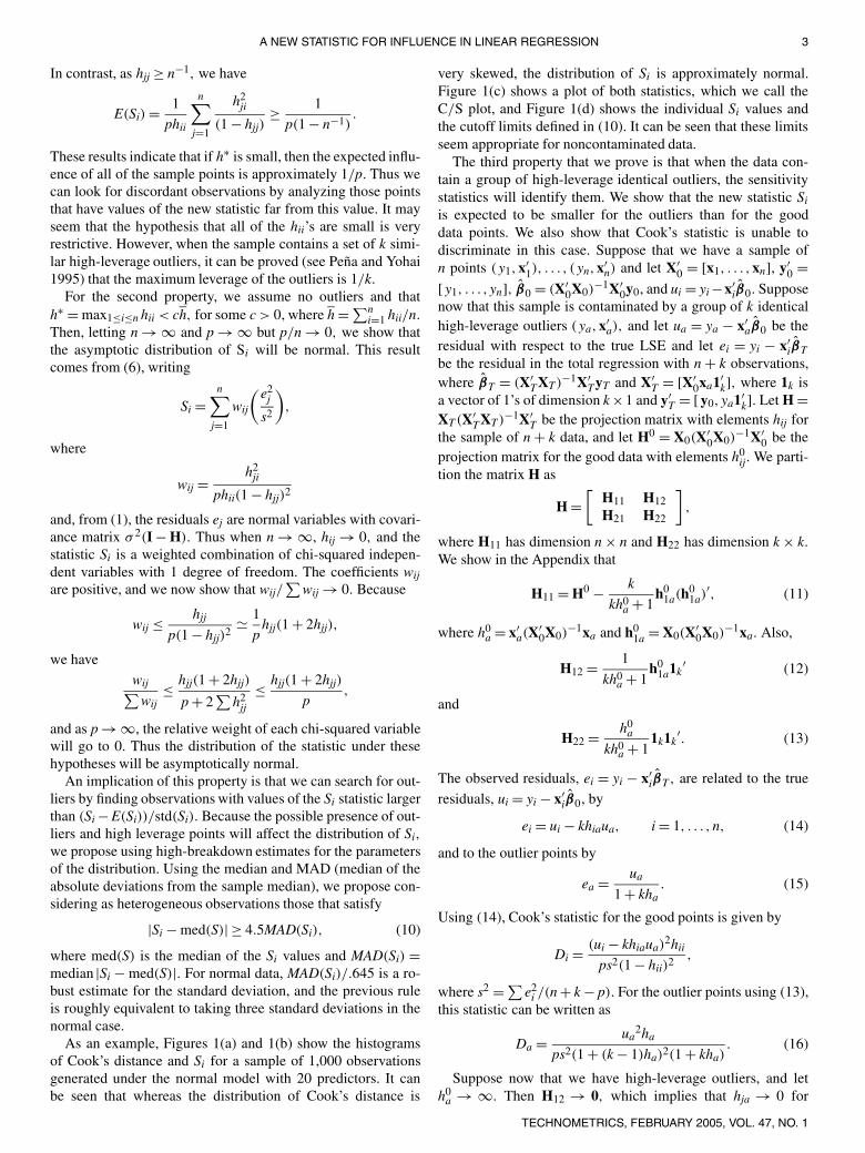
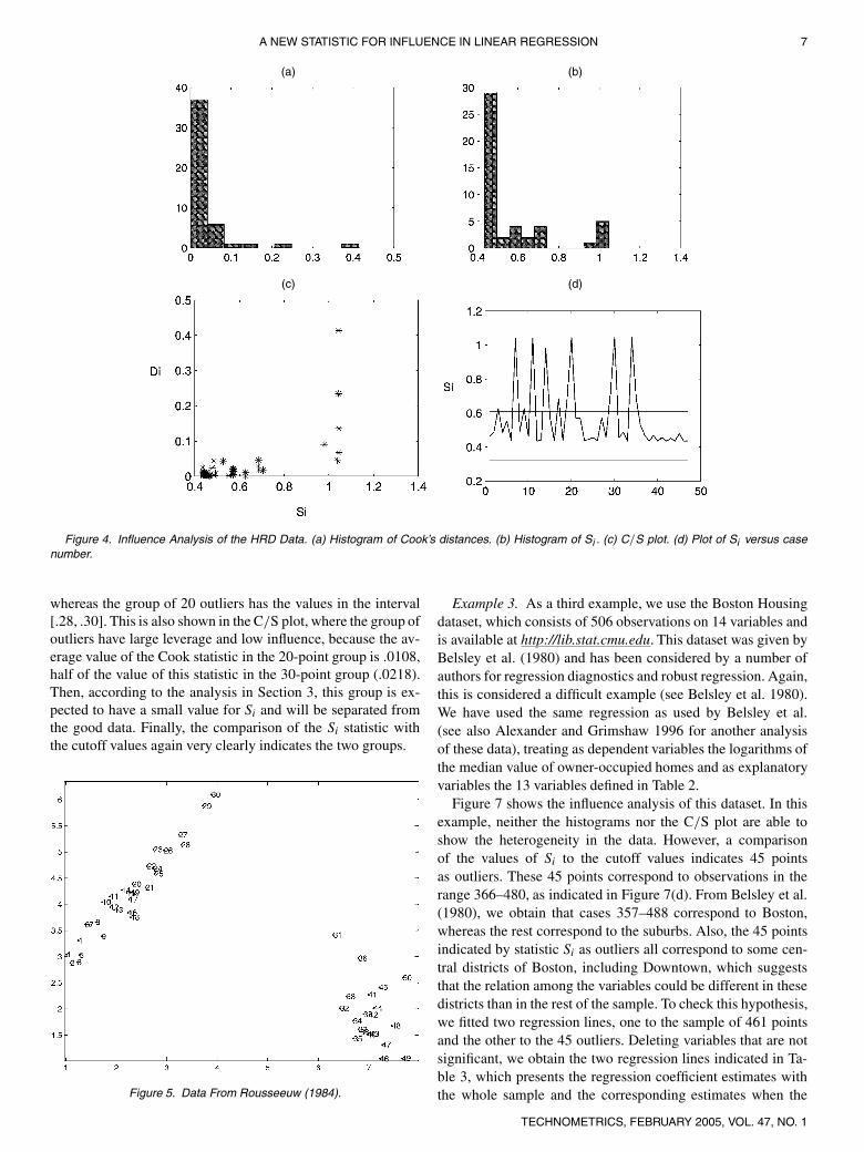