EDCN-902C-Statistic in Eduction.pdf - Tripura University
208
STATISTICS IN EDUCATION MA [Education] EDCN-902 C [ENGLISH EDITION] Directorate of Distance Education TRIPURA UNIVERSITY
-
Upload
khangminh22 -
Category
Documents
-
view
0 -
download
0
Transcript of EDCN-902C-Statistic in Eduction.pdf - Tripura University

STATISTICS IN EDUCATION
MA [Education]EDCN-902 C
[ENGLISH EDITION]
Directorate of Distance EducationTRIPURA UNIVERSITY

ReviewerR P Hooda
Vice-Chancellor of Maharishi Dayanand University (MDU), Rohtak.
Books are developed, printed and published on behalf of Directorate of Distance Education,Tripura University by Vikas Publishing House Pvt. Ltd.
All rights reserved. No part of this publication which is material, protected by this copyright noticemay not be reproduced or transmitted or utilized or stored in any form of by any means now knownor hereinafter invented, electronic, digital or mechanical, including photocopying, scanning, recordingor by any information storage or retrieval system, without prior written permission from the DDE,Tripura University & Publisher.
Information contained in this book has been published by VIKAS® Publishing House Pvt. Ltd. and hasbeen obtained by its Authors from sources believed to be reliable and are correct to the best of theirknowledge. However, the Publisher and its Authors shall in no event be liable for any errors, omissionsor damages arising out of use of this information and specifically disclaim any implied warranties ormerchantability or fitness for any particular use.
Vikas® is the registered trademark of Vikas® Publishing House Pvt. Ltd.
VIKAS® PUBLISHING HOUSE PVT. LTD.E-28, Sector-8, Noida - 201301 (UP)Phone: 0120-4078900 • Fax: 0120-4078999Regd. Office: 7361, Ravindra Mansion, Ram Nagar, New Delhi 110 055• Website: www.vikaspublishing.com • Email: [email protected]
AuthorsJ.S. Chandan, (Units: 1.2, 1.3-1.4, 2.2) © J.S. Chandan, 2017C.R. Kothari, (Units: 3.2-3.3.3, 4.2) © C.R. Kothari, 2017Dr. Harish Kumar, (Units: 4.2.1-4.2.2, 4.3.4-4.3.6, 5.2) © Dr. Harish Kumar, 2017Dr. (Mrs.) Vasantha R. Patri, (Unit: 5.3) © Dr. (Mrs.) Vasantha R. Patri, 2017Vikas Publishing House, (Units: 1.0-1.1, 1.2.1-1.2.2, 1.5-1.9, 2.0-2.1, 2.3-2.8, 3.0-3.1, 3.3.4-3.3.5, 3.4-3.8, 4.0-4.1, 4.3-4.3.3,4.4-4.8, 5.0-5.1, 5.4-5.8) © Reserved, 2017
SYLLABI-BOOK MAPPING TABLEStatistics in Education
Unit - IMeaning of Statistics: Statistis as a Tool in Educational Research.Statistical Tables, Frequency Distribution, GraphicalRepresentation of Data. Meaning Advantages and Modes ofGraphical Representation of Data.
Unit - IIMeasures of Central Tendency. Arithmetic Mean, Median Mode:Calculation, Interpretation and Use of Measures of CentralTendency. Measures of Variability-Meaning of the Measures ofVariability, Range, Quartile Deviation, Average Deviation,Standard Deviation. When and Where to Use the VariousMesaures of Variability.
Unit - IIICorrelation and Regression. Correlation-Meaning and Types.The Calculation of the Correlation by the Product MomentMethod. Linear Regression, The Regression Line in Prediction,Partial and Multiple Correlation.
Unit - IVNormal Distribution: Meaning, Significance, Characteristics ofNormal Curve. Computing Percentiles and Percentile Ranks.Standard Errors of Measurement Measuring Divergence fromNormality. Need and Importance of Significance of the Differenebetween Means and other Statistics. Null Hypothesis, Level ofConfidence, One-tailed and Two-tailed tests of Significance. TheSignificance of the Difference between Means, Percentagesand Correlation Coefficients.
Unit - VAnalysis of Variance, Non-parametric Tests. When to UseParametric and Non-Parametric Test in Education. Median Test,Mann-Whitney ‘U’ Test, Chi-square Test, Rank-differenceCorrelation.
Syllabi Mapping in Book
Unit 1: Statistics: Nature and Scope(Pages 3-38)
Unit 2: Measures of CentralTendency
(Pages 39-90)
Unit 3: Correlation and Regression(Pages 91-130)
Unit 4: Normal Distribution(Pages 131-176)
Unit 5: Analysis of Variance(Pages 177-202)


CONTENTSINTRODUCTION 1
UNIT 1 STATISTICS: NATURE AND SCOPE 3-381.0 Introduction1.1 Unit Objectives1.2 Meaning of Statistics
1.2.1 Statistics as a Tool in Educational Research1.2.2 Statistical Tables
1.3 Frequency Distribution1.4 Graphical Representation of Data: Advantages and Modes1.5 Summary1.6 Key Terms1.7 Answers to ‘Check Your Progress’1.8 Questions and Exercises1.9 Further Reading
UNIT 2 MEASURES OF CENTRAL TENDENCY 39-902.0 Introduction2.1 Unit Objectives2.2 Measures of Central Tendency: Calculation, Interpretation and Use of
Measures of Central Tendency2.2.1 Measures of Central Tendency: Arithmetic Mean, Median and Mode2.2.2 Weighted Arithmetic Mean; 2.2.3 Harmonic Mean
2.3 Measures of Variability/Dispersion: When and Where to Use the Various Measures of Variability2.3.1 Quartile Deviation (QD); 2.3.2 Average Deviation (AD)2.3.3 Standard Deviation (SD); 2.3.4 Range (R); 2.3.5 Skewness2.3.6 Kurtosis; 2.3.7 Comparison of Various Measures of Dispersion2.3.8 Coefficient of Variation
2.4 Summary2.5 Key Terms2.6 Answers to ‘Check Your Progress’2.7 Questions and Exercises2.8 Further Reading
UNIT 3 CORRELATION AND REGRESSION 91-1303.0 Introduction3.1 Unit Objectives3.2 Correlation and Regression: An Overview
3.2.1 Coefficient of Determination3.2.2 Coefficient of Correlation: Product Moment Method3.2.3 Probable Error (P.E.) of the Coefficient of Correlation3.2.4 Some Other Measures
3.3 Multiple Regression3.3.1 Linear Regression Analysis3.3.2 Checking the Accuracy of Equation: Regression Line in Prediction

3.3.3 Standard Error of the Estimate3.3.4 Predicting an Estimate, and its Preciseness3.3.5 Multiple and Partial Correlation
3.4 Summary3.5 Key Terms3.6 Answers to ‘Check Your Progress’3.7 Questions and Exercises3.8 Further Reading
UNIT 4 NORMAL DISTRIBUTION 131-1764.0 Introduction4.1 Unit Objectives4.2 Meaning, Significance and Characteristics of Normal Curve
4.2.1 Normal Probability Curve and its Uses4.2.2 Uses of Normal Probability Curve: Computing Percentiles and Percentile Ranks
4.3 Need, Importance and Significance of the Difference between Means and other Statistics4.3.1 Null Hypothesis4.3.2 Z-test4.3.3 t-Test4.3.4 Sampling Distribution of Means4.3.5 Confidence Intervals and Levels of Significance4.3.6 Two-Tailed and One-Tailed Tests of Significance
4.4 Summary4.5 Key Terms4.6 Answers to ‘Check Your Progress’4.7 Questions and Exercises4.8 Further Reading
UNIT 5 ANALYSIS OF VARIANCE 177-2025.0 Introduction5.1 Unit Objectives5.2 Analysis of Variance: Parametric Tests and When to Use Them
5.2.1 Basic Principle of ANOVA5.2.2 One-Way ANOVA5.2.3 Two-Way ANOVA
5.3 Non-parametric Tests: When to Use Non-Parametric Tests in Education5.3.1 Chi-square (χ2) Test5.3.2 Mann-Whitney U Test5.3.3 Rank-difference Methods5.3.4 Coefficient Concordance, W5.3.5 Median Test5.3.6 Kruskal-Wallis H Test5.3.7 Friedman Test
5.4 Summary5.5 Key Terms5.6 Answers to ‘Check Your Progress’5.7 Questions and Exercises5.8 Further Reading

Introduction
NOTES
Self-Instructional Material 1
INTRODUCTIONStatistics is considered a mathematical science pertaining to the collection, analysis,interpretation or explanation and presentation of data. Statistical analysis is veryimportant for taking decisions and is widely used by academic institutions, naturaland social sciences departments, governments and business organizations. Theword statistics is derived from the Latin word status which means a politicalstate or government. It was originally applied in connection with kings and monarchscollecting data on their citizenry which pertained to state wealth, collection oftaxes, study of population, and so on.
The subject of statistics is primarily concerned with making decisions aboutvarious disciplines of market and employment, such as stock market trends,unemployment rates in various sectors of industries, demographic shifts, interestrates and inflation rates over the years, as well as in education. Statistics is alsoconsidered a science that deals with numbers or figures describing the state ofaffairs of various situations with which we are generally and specifically concerned.To a layman, it often refers to a column of figures or perhaps tables, graphs andcharts relating to areas, such as population, national income, expenditures,production, consumption, supply, demand, sales, imports, exports, births, deaths,accidents, and so on. Similarly, statistical records kept at universities may reflectthe number of students, percentage of female and male students, number of divisionsand courses in each division, number of professors, tuition received, expendituresincurred, and so on.
Hence, the subject of statistics deals primarily with numerical data gatheredfrom surveys or collected using various statistical methods. Its objective is tosummarize such data, so that the summary gives us a good indication about somecharacteristics of a population or phenomenon that we wish to study. To ensurethat our conclusions are meaningful, it is necessary to subject our data to scientificanalysis so that rational decisions can be made. Thus, the field of statistics isconcerned with proper collection of data, organizing this data into manageableand presentable form, analysing and interpreting the data into conclusions for usefulpurposes.
This book is written in a self-instructional format and is divided into fiveunits. Each unit begins with an Introduction to the topic followed by an outline ofthe Unit objectives. The content is then presented in a simple and easy-to-understandmanner, and is interspersed with Check Your Progress questions to test the reader’sunderstanding of the topic. A list of Questions and Exercises is also provided atthe end of each unit, and includes short-answer as well as long-answer questions.The Summary and Key Terms section are useful tools for students and are meantfor effective recapitulation of the text.


Statistics: Nature and Scope
NOTES
Self-Instructional Material 3
UNIT 1 STATISTICS: NATURE ANDSCOPE
Structure1.0 Introduction1.1 Unit Objectives1.2 Meaning of Statistics
1.2.1 Statistics as a Tool in Educational Research1.2.2 Statistical Tables
1.3 Frequency Distribution1.4 Graphical Representation of Data: Advantages and Modes1.5 Summary1.6 Key Terms1.7 Answers to ‘Check Your Progress’1.8 Questions and Exercises1.9 Further Reading
1.0 INTRODUCTION
Statistics has become an integral part of our daily lives. Every day, we are confrontedwith some form of statistical information through newspapers, magazines and otherforms of communication. Such statistical information has become highly influentialin our lives. Indeed, the famous science fiction writer H.G. Wells had predictednearly a century ago that statistical thinking will one day be as necessary for efficientcitizenship as the ability to read and write. Thus, the subject of statistics in itself, hasgained considerable importance in affecting the processes of our thinking and decision-making.
In this unit, you will learn about the nature and scope of statistics. You willstudy statistics as a tool in educational research. You will also learn about statisticaltables, frequency distribution and the graphical representation of data.
1.1 UNIT OBJECTIVES
After going through this unit, you will be able to:• Discuss the meaning, nature and scope of statistics• Assess statistics as a tool in educational research• Explain frequency distribution and the construction of a frequency distribution• Describe the advantages and the modes of graphical representation of data

4 Self-Instructional Material
Statistics: Nature and Scope
NOTES
1.2 MEANING OF STATISTICS
In order for the quantitative and numerical data to be identified as statistics, it mustpossess certain identifiable characteristics. Some of these characteristics aredescribed below.
1. Statistics are aggregates of facts: Single or isolated facts or figures cannotbe called statistics as these cannot be compared or related to other figureswithin the same framework. Accordingly, there must be an aggregate ofthese figures. For example, if I say that I earn $30,000 per year, it would notbe considered statistics. On the other hand, if I say that the average salary ofa professor at our college is $30,000 per year, then this would be consideredstatistics since the average has been computed from many related figuressuch as yearly salaries of many professors. Similarly, a single birth in a hospitalis not statistics, as it has no significance for analytical purposes. However,when such information about many births in the same hospital or birthinformation for different hospitals is collected, then this information can becompared and analysed, and thus this data would constitute statistics.
2. Statistics, generally are not the outcome of a single cause, but areaffected by multiple causes: There are a number of forces working togetherthat affect the facts and figures. For example, when we say that the crimerate in New York city has increased by 15 per cent over the last year, anumber of factors might have affected this change. These factors may be:general level of economy such as state of economic recession, unemploymentrate, extent of use of drugs, areas affected by crime, extent of legaleffectiveness, social structure of the family in the area and so on. Whilethese factors can be isolated by themselves, the effects of these factorscannot be isolated and measured individually. Similarly, a marked increase infood grain production in India may have been due to combined effect ofmany factors such as better seeds, more extensive use of fertilizers,mechanisation in cultivation, better institutional framework and governmentaland banking support, adequate rainfall and so on. It is generally not possibleto segregate and study the effect of each of these forces individually.
3. Statistics are numerically expressed: All statistics are stated in numericalfigures which means that these are quantitative information only. Qualitativestatements are not subject to accurate interpretations and hence cannot becalled statistics. For example, qualitative statements such as India is adeveloping country or Jack is very tall would not be considered statisticalstatements. On the other hand, comparing per capita income of India withthat of America would be considered statistical in nature. Similarly, Jack’sheight in numbers compared to average height in America would also beconsidered statistics.
4. Statistical data is collected in a systematic manner: The procedures forcollecting data should be predetermined and well planned and such data

Statistics: Nature and Scope
NOTES
Self-Instructional Material 5
collection should be undertaken by trained investigators. Haphazard collectionof data can lead to erroneous conclusions.
5. Statistics are collected for a predetermined purpose: The purpose andobjective of collecting pertinent data must be clearly defined, decided uponand determined prior to data collection. This would facilitate the collection ofproper and relevant data. For example, data on the heights of students wouldbe irrelevant if considered in connection with the ability to get admission in acollege, but may be relevant when considering qualities of leadership. Similarly,collective data on the prices of commodities in itself does not serve any purposeunless we know, for the purpose of comparison, the type of commoditiesunder investigation and whether these relate to producer, distributor, wholesaleor retail prices. As another example, if you are collecting data on the numberof in-patients in the hospital waiting to be X-rayed, then the pre-determinedpurpose may be to establish the average time for the patients before X-rayand what can be done to reduce this waiting time.
6. Statistics are enumerated or estimated according to reasonablestandard of accuracy: There are basically two ways of collecting data. Oneis the actual counting or measuring, which is the most accurate way. Forexample, the number of people attending a football game can be accuratelydetermined by counting the number of tickets sold and redeemed at the gate.The second way of collecting data is by estimation and is used in situationswhere actual counting or measuring is not feasible or where it involvesprohibitive costs. For example, the crowd at the football game can be estimatedby visual observation or by taking samples of some segments of the crowdand then estimating the total number of people on the basis of these samples.Estimates based on samples cannot be as precise and accurate as actualcounts or measurements, but these should be consistent with the degree ofaccuracy desired.
7. Statistics must be placed in relation to each other: The main objectiveof data collection is to facilitate a comparative or relative study of the desiredcharacteristics of the data. In other words, the statistical data must becomparable with each other. The comparisons of facts and figures may beconducted regarding the same characteristics over a period of time from asingle source or it may be from various sources at any one given time. Forexample, prices of different items in a store as such would not be consideredstatistics. However, prices of one product in different stores constitutestatistical data, since these prices are comparable. Also, the changes in theprice of a product in one store over a period of time would also be consideredstatistical data since these changes provide for comparison over a period oftime. However, these comparisons must relate to the same phenomenon orsubject so that likes are compared with likes and oranges are not comparedwith apples.

6 Self-Instructional Material
Statistics: Nature and Scope
NOTES
Functions of StatisticsStatistics is no longer confined to the domain of mathematics. It has spread to mostof the branches of knowledge including social sciences and behavioural sciences.One of the reasons for its phenomenal growth is the variety of different functionsattributed to it. Some of the most important functions of statistics are described asfollows:
1. It condenses and summarizes voluminous data into a few presentable,understandable and precise figures: The raw data, as is usually available,is voluminous and haphazard. It is generally not possible to draw anyconclusions from the raw data as collected. Hence, it is necessary and desirableto express this data in few numerical values. For example, the average salaryof a policeman is derived from a mass of data from surveys. But just onesummarized figure gives us a pretty good idea about the income of policeofficers. Similarly, stock market prices of individual stocks and their trendsare highly complex to comprehend, but a graph of price trends gives us theoverall picture at a glance.
2. It facilitates classification and comparison of data: Arrangement of datawith respect to different characteristics, facilitates comparison andinterpretation. For example, data on age, height, sex and family income ofcollege students gives us a much better picture of students when the data iscategorized relative to these characteristics. Additionally, simply the statementsabout these figures don’t convey any significant meaning. It is their comparisonthat helps us draw conclusions.
3. It helps in determining functional relationships between two or morephenomenon: Statistical techniques such as correlational analysis assistin establishing the degree of association between two or more independentvariables. For example, the coefficient of correlation between literacy andemployment gives us the degree of association between extent of trainingand industrial productivity. Similarly, correlation between average rainfall andagricultural productivity can be obtained by using such statistical tools. Somestatistical methods can also be used in formulating and testing hypothesisabout a certain phenomenon. For example, it can be tested whether a creditsqueeze is effective in controlling prices of consumer goods or whether tenuredprofessors are more motivated to improve their teaching than untenuredprofessors.
4. It helps in predicting future trends: Statistical methods are highly usefultools in analysing the past data and predicting some future trends. For example,the sales for a particular product for the next year can be computed by knowingthe sales for the same product over the previous years, the current markettrends and the possible changes in the variables that affect the demand of theproduct.
5. It helps the central management and the government in formulatingpolicies: Various governmental policies regarding import and export trade,

Statistics: Nature and Scope
NOTES
Self-Instructional Material 7
taxation, planning, resource allocation and so on are formulated on the basisof data regarding these elements. Many other policies are based upon statisticalforecasts made by statisticians, such as policies regarding housing,employment, industrial expansion, food grain production and so on. Some ofthese policies would be based upon population forecasts for the future years.Also based upon the forecasts of future trends, events or demand, the centralorganizational management can modify their policies and plan to meet futureneeds. For example, the oil production in OPEC countries for the next fewyears would affect the operations of many energy consuming industries inAmerica. Accordingly, these organizations must plan to meet these challengesin the future.
Limitations of StatisticsThe field of statistics, though widely used in all areas of human knowledge andwidely applied in a variety of disciplines such as business, economics and research,has its own limitations. Some of these limitations are:
1. It does not deal with individual values: As discussed earlier, statisticsonly deals with aggregate values. For example, the marks obtained by onestudent in a class does not carry any meaning in itself, unless it can be comparedwith a set standard or with other students in the same class or with his ownmarks obtained earlier.
2. It cannot deal with qualitative characteristics: Statistics is not applicableto qualitative characteristics such as honesty, integrity, goodness, colour, poverty,beauty and so on, since these cannot be expressed in quantitative terms.These characteristics, however, can be statistically dealt with if somequantitative values can be assigned to these with logical criterion. For example,intelligence may be compared to some degree by comparing IQs or someother scores in certain intelligence tests.
3. Statistical conclusions are not universally true: Since statistics is not anexact science, as is the case with natural sciences, the statistical conclusionsare true only under certain assumptions. Also, the field deals extensively withthe laws of probability which at best are educated guesses. For example, ifwe toss a coin 10 times, where the chances of a head or a tail are 1:1, wecannot say with certainty that there will be 5 heads and 5 tails. Thus thestatistical laws are only approximations.
4. Statistical interpretation requires a high degree of skill andunderstanding of the subject: In order to get meaningful results, it isnecessary that the data be properly and professionally collected and criticallyinterpreted. It requires extensive training to read and analyse statistics in itsproper context. It may lead to fallacious conclusions in the hands of theinexperienced.
5. Statistics can be misused: The famous statement that figures don’t liebut the liars can figure, is a testimony to the misuse of statistics. Thus,inaccurate or incomplete figures, can be manipulated to get desirable

8 Self-Instructional Material
Statistics: Nature and Scope
NOTES
references. For example, the profits for company X being $100,000 in a givenyear are not necessarily inferior to profits of a company Y being $150,000,unless we know the size of the company and their total sales. Similarly,advertising slogans such as 4 out of 5 dentists recommend brand X toothpaste gives us the impression that 80 per cent of all dentists recommend thisbrand. This may not be true since we don’t know how big the sample is orwhether the sample represents the entire population or not. Accordingly, suchstatistical conclusions can be highly misleading. Statements like, statisticscan prove anything and there are three types of lies — lies, damned liesand statistics, perhaps, do have a profound basis.
Scope of StatisticsThere is hardly any walk of life which has not been affected by statistics—rangingfrom a simple household to big businesses and the government. Some of the importantareas where the knowledge of statistics is usefully applied are as follows:
1. Government: Since the beginning of organized society, the rulers and theheads of states have relied heavily on statistics in the form of collecting dataon various aspects for formulating sound military and fiscal policies. Thisdata may have involved population, taxes collected, military strength and soon. In the current structure of democratic societies, the government is, perhaps,the biggest collector of data and user of statistics. Various departments of thegovernment collect and interpret vast amount of data and information forefficient functioning and decision-making.
2. Economics: Statistics are widely used in economics study and research.The subject of economics is mainly concerned with production and distributionof wealth as well as savings and investments. Some of the areas of economicinterest in which statistical tools are used are as follows:
(a) Statistical methods are extensively used in measuring and forecastingGross National Product (GNP).
(b) Economic stability is primarily judged by statistical studies of businesscycles.
(c) Statistical analyses of population growth, unemployment figures, ruralor urban population shifts and so on influence much of the economicpolicy making.
(d) Econometric models which involve application of statistical methodsare used for optimum utilisation of resources available.
(e) Financial statistics are necessary in the fields of money and bankingincluding consumer savings and credit availability.
3. Physical, natural and social sciences: In physical sciences, as an example,the science of meteorology uses statistics in analysing the data gathered bysatellites in predicting weather conditions. Similarly, in botany, in the naturalsciences, statistics are used in evaluating the effects of temperature andother climatic conditions and types of soil on the health of plants. In the social

Statistics: Nature and Scope
NOTES
Self-Instructional Material 9
sciences, ‘statistics are extensively used in all areas of human and socialcharacteristics.’
4. Statistics and research: There is hardly any advanced research going onwithout the use of statistics in one form or another. Statistics are usedextensively in medical, pharmaceutical and agricultural research. Theeffectiveness of a new drug is determined by statistical experimentation andevaluation. In agricultural research, experiments about crop yields, types offertilizers and types of soils under different types of environments arecommonly designed and analysed through statistical methods. In marketingresearch, statistical tools are indispensable in studying consumer behaviour,effects of various promotional strategies and so on.
5. Other areas: Statistics are commonly used by insurance companies, stockbrokerage houses, banks, public utility companies and so on. Statistics arealso immensely useful to politicians since they can predict their chances forwinning through the use of sampling techniques in random selection of votersamples and studying their attitudes on issues and policies.
Statistics in Business and ManagementStatistics influence the operations of business and management in many dimensions.Statistical applications include the area of production, marketing, promotion of product,financing, distribution, accounting, marketing research, manpower planning,forecasting, research and development and so on. As the organizational structurehas become more complex and the market highly competitive, it has become necessaryfor executives to base their decisions on the basis of elaborate information systemsand analysis instead of intuitive judgement. In such situations, statistics are used toanalyse this vast data base for extracting relevant information. Some of the typicalareas of business operations where statistics have been extensively and effectivelyused are as follows:
1. Entrepreneuring: If you are opening a new business or acquiring one, it isnecessary to study the market as well as the resources from statistical pointof view to ensure success of the new venture. A shrewd businessman mustmake a proper and scientific analysis of the past records and current markettrends in order to predict the future course for business conditions. The analysisof the needs and wants of the consumers, the number of competitors in themarket and their marketing strategies, availability of resources and generaleconomic conditions and trends would all be extremely helpful to theentrepreneur. A number of new enterprises have failed either due to unreliabilityof data or due to faulty interpretations and conclusions.
2. Production: The production of any item depends upon the demand of thatitem and this demand must be accurately forecast using statistical techniques.Similarly, decisions as to what to produce and how much to produce arebased largely upon the feedback of surveys that are analysed statistically.
3. Marketing: An optimum marketing strategy would require a skillful analysisof data on population, shifts in population, disposable income, competition,

10 Self-Instructional Material
Statistics: Nature and Scope
NOTES
social and professional status of target market, advertising, quality of salespeople, easy availability of the product and other related matters. Thesevariables and their inter-relationships must be statistically studied and analysed.
4. Purchasing: The purchasing department of an organization makes decisionsregarding the purchase of raw materials and other supplies from differentvendors. The statistical data in the cost structure would assist in formulatingpurchasing policies as to where to buy, when to buy, at what price to buy andhow much to buy at a given time.
5. Investment: Statistics have been almost indispensable in making a soundinvestment whether it be in buying or selling of stocks and securities or realestate. The financial newspapers are full of tables and graphs analysing theprices of stocks and their movements. Based upon these statistical data, agood investor will buy when the prices are at their lowest and sell when theprices are at their highest. Similarly, buying an apartment building would requirethat an investor take into consideration the rent collected, rate of occupancy,any rent control laws, cost of the mortgage obtained and the age of the buildingbefore making a decision about investing in real estate.
6. Banking: Banks are highly affected by general economic and marketconditions. Many banks have research departments which gather and analyseinformation not only about general economic conditions but also aboutbusinesses in which they may be directly or indirectly involved. They must beaware of money markets, inflation rates, interest rates and so on, not only intheir own vicinity but also nationally and internationally. Many banks havelost money in international operations, sometimes in as simple a matter ascurrency fluctuations because they did not analyse the international economictrends correctly. Many banks have failed because they over-extendedthemselves in making loans without properly analysing the general businessconditions.
7. Quality control: Statistics are used in quality control so extensively thateven the phenomenon itself is known as statistical quality control. Statisticalquality control (SQC) consists of using statistical methods to gather and analysedata on the determination and control of quality. This technique primarilydeals with the samples taken randomly and as representative of the entirepopulation, then these samples are analysed and inferences made concerningthe characteristics of the population from which these random samples weretaken. The concept is similar to testing one spoonful from a pot of stew anddeciding whether it needs more salt or not. The characteristics of samplesare analysed by statistical quality control and the use of other statisticaltechniques.
8. Personnel: Study of statistical data regarding wage rates, employment trends,cost of living indexes, work related accident rates, employee grievances, labourturnover rates, records of performance appraisal and so on and the properanalysis of such data assist the personnel departments in formulating thepersonnel policies and in the process of manpower planning.

Statistics: Nature and Scope
NOTES
Self-Instructional Material 11
As we have seen, statistics in one form or another, affects every businessand every individual. An average individual is involved in statistics, knowingly orunknowingly, every day of his life; whether it be comparing prices during shoppingor putting an extra lock on his door as a result of reading the crime rate in thenewspapers. Perhaps, it is an exaggeration but basically it is true what anoverenthusiastic, statistically aware business executive stated many years ago, Whenthe history of modern times is finally written, we shall read it as beginning withthe age of steam and progressing through the age of electricity to that ofstatistics.
1.2.1 Statistics as a Tool in Educational Research
A researcher needs to be familiar with the various statistical methods so as to beable to use the appropriate method in his research study. There are certain basicstatistical methods, which can be classified into three groups as follows:
• Descriptive statistics• Inferential statistics• Measures of central tendency and dispersion
Descriptive StatisticsAccording to Smith, descriptive statistics is the formulation of rules and procedureswhere data can be placed in a useful and significant order. The foundation ofapplicability of descriptive statistics is the need for complete data presentation. Themost important and general methods used in descriptive statistics are as follows:
• Ratios: This indicates the relative frequency of the various variables to oneanother.
• Percentages: Percentages (%) can be derived by multiplying a ratio with100. It is thus a ratio representing a standard unit of 100.
• Frequency table: It is a means to tabulate the rate of recurrence of data.Data arranged in such a manner is known as ‘distribution’. In case of a largedistribution tendency, larger class intervals are used. This facilitates theresearcher to acquire a more orderly system.
• Histogram: It is the graphical representation of a frequency distributiontable. The main advantage of graphical representation of data in the form ofhistogram is that data can be interpreted immediately.
• Frequency polygon: It is used for the representation of data in the form ofa polygon. In this method, a dot that represents the highest score is placed inthe middle of the class interval. A frequency polygon is derived by linkingthese dots. An additional class is sometimes added in the end of the line withthe purpose of creating an anchor.
• Cumulative frequency curve: The procedure of frequency involves addingfrequency by starting from the bottom of the class interval, and adding classby class. This facilitates the representation of the number of persons that

12 Self-Instructional Material
Statistics: Nature and Scope
NOTES
perform below the class interval. The researcher can derive a curve from thecumulative frequency tables with the purpose of reflecting data in a graphicalmanner.
Inferential StatisticsInferential statistics enable researchers to explore unknown data. Researchers canmake deductions or statements using inferential statistics with regard to the broadpopulation from which samples of known data has been drawn. These methods arecalled ‘inferential or inductive statistics’. These methods include the followingcommon techniques:
• Estimation: It is the calculated approximation of a result, which is usable,even if the input data may be incomplete or uncertain. It involves deriving theapproximate calculation of a quantity or a degree or worth. For example,drawing an estimate of cost of a project or deriving a rough idea of how longthe project would take.
• Prediction: It is a statement or claim that a particular event will surely occurin future. It is based on observation, experience and scientific reasoning ofwhat will happen in given circumstances or situations.
• Hypothesis testing: Hypothesis is a proposed explanation, whose validitycan be tested. Hypothesis testing attempts to validate or disprove preconceivedideas. In creating hypothesis, one thinks of a possible explanation for aremarked behaviour. The hypothesis dictates the data selected to be analysedfor further interpretations.There are also two chief statistical methods based on the tendency of data to
cluster or scatter. These methods, known as measures of central tendency andmeasures of dispersion, have been discussed in the next sub-section.
1.2.2 Statistical Tables
Most research studies involve some form of numerical data, and even though onecan discuss this in text, it is best represented in tabular form. The advantage of doingthis is that statistical tables present the data in a concise and numeral form, whichmakes quantitative analysis and comparisons easier. Tables formulated could begeneral tables following a statistical format for a particular kind of analysis. Theseare best put in the appendix, as they are complex and detailed in nature. The otherkind is simple summary tables, which only contain limited information and yet, are,essentially critical to the report text.
The mechanics of creating a summary table are very simple and are illustratedbelow with an example (Table 1.1). The illustration has been labelled with numberswhich relate to the relevant section.

Statistics: Nature and Scope
NOTES
Self-Instructional Material 13
Table 1.1 Automobile Domestic Sales Trends
Table identification details: The table must have a title (1a) and anidentification number (1b). The table title should be short and usually would notinclude any verbs or articles. It only refers to the population or parameter beingstudied. The title should be briefly yet clearly descriptive of the information provided.The numbering of tables is usually in a series and generally one makes use of Arabicnumbers to identify them.
Data arrays: The arrangement of data in a table is usually done in an ascendingmanner. This could either be in terms of time, as shown in Table 1.1 (column-wise) oraccording to sectors or categories (row-wise) or locations, e.g., north, south, east,west and central. Sometimes, when the data is voluminous, it is recommended thatone goes alphabetically, e.g., country or state data. Sometimes there may be subcategoriesto the main categories, for example, under the total sales data—a columnwisecomponent of the revenue statement—there could be subcategories of departmentstore, chemists and druggists, mass merchandisers and others. Then these have to bedisplayed under the sales data head, after giving a tab command as follows:
Total salesMass marketDepartment storeDrug storesOthers (including paan beedi outlets)Measurement unit: The unit in which the parameter or information is
presented should be clearly mentioned.Spaces, leaders and rulings (SLR): For limited data, the table need not be
divided using grid lines or rulings, simple white spaces add to the clarity of informationpresented and processed. In case the number of parameters are too many and thedata seems to be bulky to be simply separated by space, it is advisable to use verticalruling. Horizontal lines are drawn to separate the headings from the main data, ascan be seen in Table 1.1. When there are a number of subheadings as in the sales

14 Self-Instructional Material
Statistics: Nature and Scope
NOTES
data example, one may consider using leaders (…….) to assist the eye movement inabsorbing and processing the information.
Total salesMass market………Department store………Drug stores………Others (including paan beedi outlets)………Assumptions, details and comments: Any clarification or assumption
made, or a special definition required to understand the data, or formula used toarrive at a particular figure, e.g., total market sale or total market size can be givenafter the main tabled data in the form of footnotes.
Data sources: In case the information documented and tabled is secondaryin nature, complete reference of the source must be cited after the footnote, if any.
Special mention: In case some figure or information is significant and thereader should pay special attention to it, the number or figure can be bold or can behighlighted to increase focus.
CHECK YOUR PROGRESS
1. What is descriptive statistics?2. What does hypothesis testing attempt to validate?3. What are the table identification details?
1.3 FREQUENCY DISTRIBUTION
Statistical data can be organized into a frequency distribution which simply lists thevalue of the variable and frequency of its occurrence in a tabular form. A frequencydistribution can be defined as the list of all the values obtained in the data and thecorresponding frequency with which these values occur in the data.
The frequency distribution can either be ungrouped or grouped. When thenumber of values of the variable is small, then we can construct an ungroupedfrequency distribution which is simply listing the frequency of occurrence againstthe value of the given variable. As an example, let us assume that 20 families weresurveyed to find out how many children each family had. The raw data obtainedfrom the survey is as follows:
0, 2, 3, 1, 1, 3, 4, 2, 0, 3, 4, 2, 2, 1, 0, 4, 1, 2, 2, 3This data can be classified into an ungrouped frequency distribution. The number ofchildren becomes our variable (X) for which we can list the frequency ofoccurrence (f) in a tabular form as follows:
Statistics: Nature and Scope
NOTES
Self-Instructional Material 15
Table 1.2 Frequency of Occurrence
Number of Children (X) Frequency (f)
0 3
1 4
2 6
3 4
4 3
Total = 20
The above table is also known as discrete frequency distribution where the variablehas discrete numerical values.However, when the data set is very large, it becomes necessary to condense thedata into a suitable number of groups or classes of the variable values and thenassign the combined frequencies of these values into their respective classes. As anexample, let us assume that 100 employees in a factory were surveyed to find outtheir ages. The youngest person was 20 years of age and the oldest was 50 yearsold. We can construct a grouped frequency distribution for this data so that insteadof listing frequency by every year of age, we can list frequency according to an agegroup. Also, since age is a continuous variable, a frequency distribution would be asfollows:
Table 1.3 Frequency Distribution
Age Group (Years) Frequency
20 to less than 25 525 ” ” ” 30 1530 ” ” ” 35 2535 ” ” ” 40 3040 ” ” ” 45 1545 ” ” ” 50 10
Total = 100
In this example, all persons between 20 years (including 20 years old) and 25 years(but not including 25 years old) would be grouped into the first class and so on. Theinterval of 20 to less than 25 is known as class interval (CI). A single representationof a class interval would be the midpoint (or average) of that class interval. Themidpoint is also known as the class-mark.
Constructing a Frequency DistributionThe number of groups and the size of class interval are more or less arbitrary innature within the general guidelines established for constructing a frequencydistribution. The following guidelines for such a construction may be considered:

16 Self-Instructional Material
Statistics: Nature and Scope
NOTES
(i) The classes should be clearly defined and each of the observations should beincluded in only one of the class intervals. This means that the intervals shouldbe chosen in such a manner that one score cannot belong to more than oneclass interval, so that there is no overlapping of class intervals.
(ii) The number of classes should neither be too large nor too small. Normally,between 6 and 15 classes are considered to be adequate. Fewer class intervalswould mean a greater class interval width with consequent loss of accuracy.Too many class intervals result in a greater complexity.
(iii) All intervals should be of the same width. This is preferred for easycomputations. A suitable class width can be obtained by knowing the range ofdata (which is the absolute difference between the highest value and thelowest value in the data) and the number of classes which are predetermined,so that:
RangeThe width of the interval =Number of classes
In the case of ages of factory workers where the youngest worker was 20years old and the oldest was 50 years old, the range would be 50–20 = 30. Ifwe decide to make 10 groups then the width of each class would be:
30/10 = 3Similarly, if we decide to make 6 classes instead of 10, then the width of eachclass interval would be:
30/6 = 5(iv) Open-ended cases where there is no lower limit of the first group or no upper
limit of the last group should be avoided since this creates difficulty in analysisand interpretation. (The lower and upper values of a class interval are knownas lower and upper limits.)
(v) Intervals should be continuous throughout the distribution. For example, in thecase of factory workers, we could group them in groups of 20 to 24 years,then 25 to 29 years, and so on, but it would be highly misleading because itdoes not accurately represent the person who is between 24 and 25 years orbetween 29 and 30 years, and so on. Accordingly, it is more representative togroup them as: 20 years to less than 25 years, 25 years to less than 30 years.In this way, everybody who is 20 years and a fraction less than 25 years isincluded in the first category and the person who is exactly 25 years andabove but a fraction less than 30 years would be included in the secondcategory, and so on. This is especially important for continuous distributions.
(vi) The lower limits of class intervals should be simple multiples of the intervalwidth. This is primarily for the purpose of simplicity in construction andinterpretation. In our example of 20 years but less than 25 years, 25 years butless than 30 years, and 30 years but less than 35 years, the lower limit valuesfor each class are simple multiples of the class width which is 5.

Statistics: Nature and Scope
NOTES
Self-Instructional Material 17
Example 1.1: A sample of 30 persons showed their ages (in years) as:20, 18, 25, 68, 23, 25, 16, 22, 29, 37,35, 49, 42, 65, 37, 42, 63, 65, 49, 42,53, 48, 65, 72, 69, 57, 48, 39, 58, 67.
Construct a frequency distribution for this data.
Solution:Follow the steps as given below:
1. Find the range of the data by subtracting the lowest age from the highest age.The lowest value is 16 and the highest value is 72. Hence, the range is72–16 = 56.
2. Assume that we shall have 6 classes, since the number of values is not toolarge. Now we divide the range of 56 by 6 to get the width of the classinterval. The width is 56/6 = 9.33. For the sake of convenience, assume thewidth to be 10 and start the first class boundary with 15 so that the intervalswould be 15 and upto 25, 25 and upto 35, and so on.
3. Combine all the frequencies that belong to each class interval and assign thistotal frequency to the corresponding class interval as follows:
Table 1.4 Class Intervals
Class Interval (Years) Tally Frequency ( f )
15 to less than 25 |||| 5
25 to less than 35 ||| 3
35 to less than 45 |||| || 7
45 to less than 55 |||| 5
55 to less than 65 ||| 3
65 to less than 75 |||| || 7
Total = 30
Discrete list conversion to a continuous listIn statistics, calculations are performed by arranging the large raw (ungrouped)data set into grouped data and are represented in tabular form called frequencydistribution table. The data to be grouped must be homogenous and comparable.The frequency distribution table gives the size and the number of class intervals.The range of each class is defined by the class boundaries.
The variables constitute either a discrete list or a continuous list. A variable isconsidered as continuous when it can assume an infinite number of real values andit is considered discrete when it is the finite number of real values. Examples of acontinuous variable are distance, age, temperature and height measurements, whereas

18 Self-Instructional Material
Statistics: Nature and Scope
NOTES
the examples of a discrete variable are the scores given by the experts or the judgementteam for competition examination, basket ball match, cricket match, etc.
For a discrete list of data, the range can be defined as 0 – 4, 5 – 9, 10 – 14,and so on. Similarly, the range of data for a continuous list can be defined as 10 – 20,20 – 30, 30 – 40, and so on.
In a class interval, the endpoints define the lowest and highest values that avariable can take. In this example, if we consider the data set for age then the classintervals are 0 to 4 years, 5 to 9 years, 10 to 14 years, and 14 years and above. Fora discrete variable, the end points, of the first class interval are 0 and 4 but for acontinuous variable it will be 0 and 4.999. In this way, the discrete variables can beconverted to continuous variables and vice versa.
Conversion of ungrouped list into grouped listThe data collected first-hand for any statistical evaluation is considered as raw orungrouped data as it is not meaningful and does not present a clear picture. It is thenarranged in the ascending or the descending order in a tabular form called array.The following example will make the concept more clear.Example 1.2: The following table shows the daily wages (in `) of 40 workers.Convert the ungrouped data into grouped data and also prepare a discrete frequencytable with tally marks.
Ungrouped Data
90 85 50 70 55 86 60 75 80 65 75 78 86 80 60 90 55 95 65 85 55 70 60 85 80 95 90 75 60 86 60 95 85 70 65 55 86 90 80 78
Solution:After arranging this into grouped data, we get the following table:
95 95 95 90 90 90 90 86 86 86 86 85 85 85 85 80 80 80 80 78 78 75 75 75 70 70 70 65 65 65 60 60 60 60 60 55 55 55 55 50

Statistics: Nature and Scope
NOTES
Self-Instructional Material 19
The discrete frequency distribution of daily wages with tally marks:
Table 1.5 Descrete Frequency Distribution
Daily Wages
Tally Marks Frequency
95 3 90 4 86 4 85 4 80 4 78 2
75 3 70 3
65 3 60 5
55 4 50 1 Total 40
Class intervals of unequal widthFrom the data given in Example 1.2, a table showing class intervals of unequal withis drawn.
Table 1.6 Class Invervals of Unequal
Daily Wages
Tally Marks Frequency
50–55 |||| 5
55–60 |||| 5
60–65 ||| 3
65–70 ||| 3
70–75 ||| 3
75–78 || 2
78–80 |||| 4
80–85 |||| 4
85–86 |||| 4
86–90 |||| 4
90–95 ||| 3
Total 40
20 Self-Instructional Material
Statistics: Nature and Scope
NOTES
Cumulative FrequencyWhile the frequency distribution table tells us the number of units in each class interval,it does not tell us directly the total number of units that lie below or above the specifiedvalues of class intervals. This can be determined from a cumulative frequencydistribution. When the interest of the investigator focusses on the number of itemsbelow a specified value, then this specified value is the upper limit of the class interval.It is known as less than cumulative frequency distribution. Similarly, when the interestlies in finding the number of cases above a specified value, then this value is taken asthe lower limit of the specified class interval and is known as more than cumulativefrequency distribution. The cumulative frequency simply means summing up theconsecutive frequencies as follows (taking the example of ages of 30 workers):
Table 1.7 Cumulative Frequency Distribution
Class Interval (Years) ( f ) Cumulative Frequency (Less Than)
15 and upto 25 5 5 (less than 25)
25 and upto 35 3 8 (less than 35)
35 and upto 45 7 15 (less than 45)
45 and upto 55 5 20 (less than 55)
55 and upto 65 3 23 (less than 65)
65 and upto 75 7 30 (less than 75)
Similarly, the following is the greater than cumulative frequency distribution:
Table 1.8 Greater than Cumulative Frequency Distribution
Class Interval (Years) ( f ) Cumulative Frequency (Greater Than)
15 and upto 25 5 30 (greater than 15)
25 and upto 35 3 25 (greater than 25)
35 and upto 45 7 22 (greater than 35)
45 and upto 55 5 15 (greater than 45)
55 and upto 65 3 10 (greater than 55)
65 and upto 75 7 7 (greater than 65)
In the preceding greater than cumulative frequency distribution; 30 persons areolder than 15, 25 are older than 25, and so on.
Percentage FrequencyThe frequency distribution, as defined earlier, is a summary table in which the originaldata is condensed into groups and their frequencies. But if a researcher would liketo know the proportion or the percentage of cases in each group, instead of simplythe number of cases, he can do so by constructing a relative frequency distributiontable. The relative frequency distribution can be formed by dividing the frequency ineach class of the frequency distribution by the total number of observations. It can

Statistics: Nature and Scope
NOTES
Self-Instructional Material 21
be converted into a percentage frequency distribution by simply multiplying eachrelative frequency by 100.
The relative frequencies are particularly helpful when comparing two or morefrequency distributions in which the number of cases under investigation is not equal.The percentage distributions make such a comparison more meaningful, sincepercentages are relative frequencies and hence the total number in the sample orpopulation under consideration becomes irrelevant. Carrying on with the earlier example:
Table 1.9 Percentage Frequency
Class Interval (Years) ( f ) Rel. Freq. % Freq.
15 and upto 25 5 5/30 16.7
25 and upto 35 3 3/30 10.0
35 and upto 45 7 7/30 23.3
45 and upto 55 5 5/30 16.7
55 and upto 65 3 3/30 10.0
65 and upto 75 7 7/30 23.3
Total 30 100.0
Cumulative relative frequency distributionIt is often useful to know the proportion or the percentage of cases falling below aparticular score point or falling above a particular score point. A less than cumulativerelative frequency distribution shows the proportion of cases lying below the upperlimit of specific class interval. Similarly, a greater than cumulative frequency distributionshows the proportion of cases above the lower limit of a specified class interval. Wecan develop the cumulative relative frequency distributions from the less than andgreater than cumulative frequency distributions constructed earlier. By followingthe earlier example, we get:
Table 1.10 Cumulative Relative Frequency Distribution
Class Interval (Years) Cum. Freq. Cum. Rel. Freq.(Less Than) (Less Than)
Less than 25 5 5/30 or 16.7%
Less than 35 8 8/30 or 26.7%
Less than 45 15 15/30 or 50.0%
Less than 55 20 20/30 or 66.7%
Less than 65 23 23/30 or 76.7%
Less than 75 30 30/30 or 100%
In the above example, 5 out of 30 or 16.7 per cent of the persons are below 25 yearsof age. Similarly, 15 out of 30 or 50 per cent of the persons are below 45 years of
22 Self-Instructional Material
Statistics: Nature and Scope
NOTES
age and so on. Similarly, we can construct a greater than cumulative relativefrequency distribution as follows for the same example:
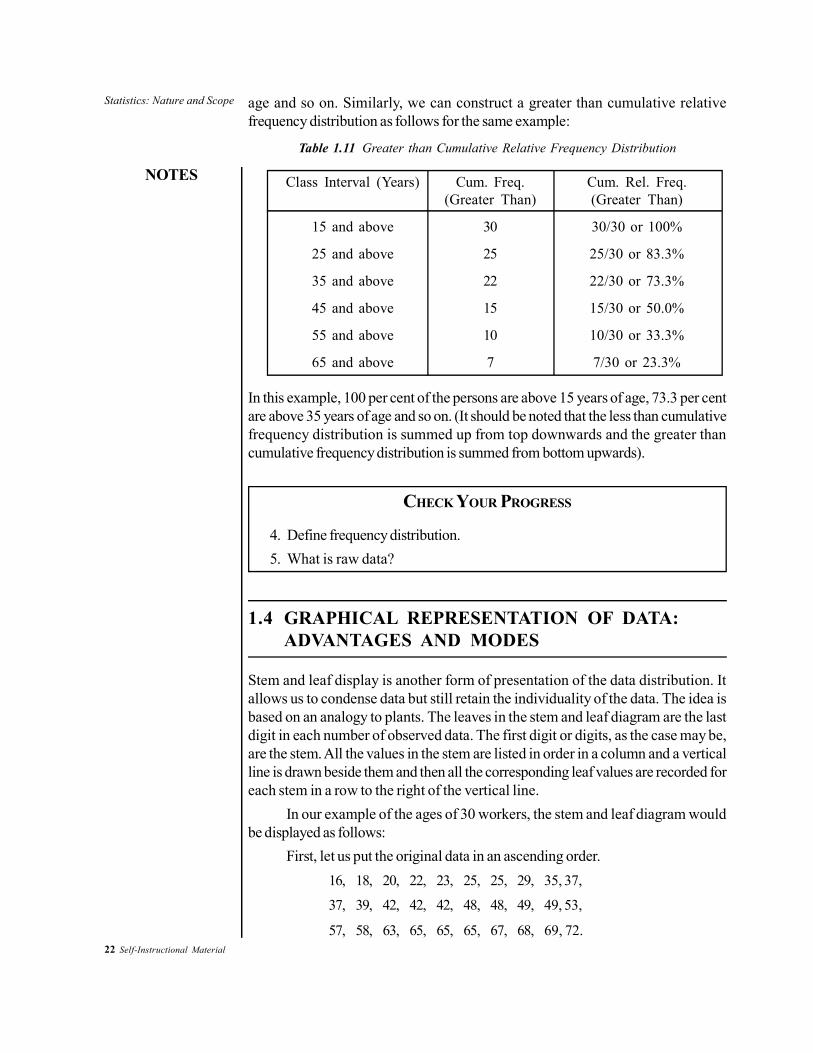
Table 1.11 Greater than Cumulative Relative Frequency Distribution
Class Interval (Years) Cum. Freq. Cum. Rel. Freq.(Greater Than) (Greater Than)
15 and above 30 30/30 or 100%
25 and above 25 25/30 or 83.3%
35 and above 22 22/30 or 73.3%
45 and above 15 15/30 or 50.0%
55 and above 10 10/30 or 33.3%
65 and above 7 7/30 or 23.3%
In this example, 100 per cent of the persons are above 15 years of age, 73.3 per centare above 35 years of age and so on. (It should be noted that the less than cumulativefrequency distribution is summed up from top downwards and the greater thancumulative frequency distribution is summed from bottom upwards).
CHECK YOUR PROGRESS
4. Define frequency distribution.5. What is raw data?
1.4 GRAPHICAL REPRESENTATION OF DATA:ADVANTAGES AND MODES
Stem and leaf display is another form of presentation of the data distribution. Itallows us to condense data but still retain the individuality of the data. The idea isbased on an analogy to plants. The leaves in the stem and leaf diagram are the lastdigit in each number of observed data. The first digit or digits, as the case may be,are the stem. All the values in the stem are listed in order in a column and a verticalline is drawn beside them and then all the corresponding leaf values are recorded foreach stem in a row to the right of the vertical line.
In our example of the ages of 30 workers, the stem and leaf diagram wouldbe displayed as follows:
First, let us put the original data in an ascending order.16, 18, 20, 22, 23, 25, 25, 29, 35, 37,
37, 39, 42, 42, 42, 48, 48, 49, 49, 53,
57, 58, 63, 65, 65, 65, 67, 68, 69, 72.

Statistics: Nature and Scope
NOTES
Self-Instructional Material 23
Now the stem and leaf diagram:
Table 1.12 Stem and Leaf
Stem Leaves ( f )
1 6 8 2
2 0 2 3 5 5 9 6
3 5 7 7 9 4
4 2 2 2 8 8 9 9 7
5 3 7 8 3
6 3 5 5 5 7 8 9 7
7 2 1
Total = 30
Summing up the frequencies provides a check on whether all the data has beenincluded or not.
Diagrammatic and Graphic PresentationThe data we collect can often be more easily understood for interpretation if it ispresented graphically or pictorially. Diagrams and graphs give visual indications ofmagnitudes, groupings, trends and patterns in the data. These important features aremore simply presented in the form of graphs. Also, diagrams facilitate comparisonsbetween two or more sets of data.
The diagrams should be clear and easy to read and understand. Too muchinformation should not be represented through the same diagram; otherwise, it maybecome cumbersome and confusing. Each diagram should include a brief and self-explanatory title dealing with the subject matter. The scale of the presentation shouldbe chosen in such a way that the resulting diagram is of appropriate size. Theintervals on the vertical as well as the horizontal axis should be of equal size; otherwise,distortions would occur.
Diagrams are more suitable to illustrate discrete data, while continuous datais better represented by graphs. The following are the diagrammatic and graphicrepresentation methods that are commonly used.
Diagrammatic RepresentationDiagrammatic representation can be of the following types:
(i) Bar diagram(ii) Pie chart(iii) Pictogram(i) Bar diagram: Bars are simply vertical lines where the lengths of the bars
are proportional to their corresponding numerical values. The width of thebar is unimportant but all bars should have the same width so as not to confusethe reader of the diagram. Additionally, the bars should be equally spaced.

24 Self-Instructional Material
Statistics: Nature and Scope
NOTES
Example 1.3: Suppose that the following were the gross revenues (in $100,000.00)for a company XYZ for the years 1989, 1990 and 1991.
Year Revenue1989 1101990 951991 65
Construct a bar diagram for this data.
Solution:
The bar diagram for this data can be constructed as follows with the revenuesrepresented on the vertical axis and the years represented on the horizontal axis.
Fig. 1.1 Bar Diagram
The bars drawn can be subdivided into components depending upon the type ofinformation to be shown in the diagram. This will be clear by the following examplein which we are presenting three components in a bar.Example 1.4: Construct a subdivided bar chart for the three types of expenditures indollars for a family of four for the years 1988, 1989, 1990 and 1991 as given as follows:
Year Food Education Other Total
1988 3000 2000 3000 80001989 3500 3000 4000 105001990 4000 3500 5000 125001991 5000 5000 6000 16000

Statistics: Nature and Scope
NOTES
Self-Instructional Material 25
Solution:
The subdivided bar chart would be as follows:
Fig. 1.2 Sub-Divided Bar Diagram
(ii) Pie chart: This type of diagram enables us to show the partitioning of a totalinto its component parts. The diagram is in the form of a circle and is alsocalled a pie because the entire diagram looks like a pie and the componentsresemble slices cut from it. The size of the slice represents the proportion ofthe component out of the whole.
Example 1.5: The following figures relate to the cost of the construction of ahouse. The various components of cost that go into it are represented as percentagesof the total cost.
Item % Expenditure
Labour 25
Cement, Bricks 30
Steel 15
Timber, Glass 20
Miscellaneous 10
Construct a pie chart for the above data.

26 Self-Instructional Material
Statistics: Nature and Scope
NOTES
Solution:
The pie chart for this data is presented as follows:
Cement, bricks30%
Labour25%
Misc.10%
Steel15%
Timber, glass20%
Fig. 1.3 Pie Chart
Pie charts are very useful for comparison purposes, especially when thereare only a few components. If there are too many components, it may becomeconfusing to differentiate the relative values in the pie.
(iii) Pictogram: Pictogram means presentation of data in the form of pictures. Itis quite a popular method used by governments and other organizations forinformational exhibitions. Its main advantage is its attractive value. Pictogramsstimulate interest in the information being presented.News magazines are very fond of presenting data in this form. For example,
in comparing the strength of the armed forces of USA and Russia, they will simplymake sketches of soldiers where each sketch may represent 100,000 soldiers. Similarcomparison for missiles and tanks is also done.
Graphic RepresentationGraphic representation can be of the following types:
(i) Histogram(ii) Frequency polygon(iii) Cumulative frequency curve (Ogive)
Each of these is briefly explained and illustrated.(i) Histogram: A histogram is the graphical description of data and is constructed
from a frequency table. It displays the distribution method of a data set andis used for statistical as well as mathematical calculations.The word histogram is derived from the Greek word histos which means‘anything set upright’ and gramma which means ‘drawing, record, writing’. Itis considered as the most important basic tool of statistical quality control process.In this type of representation, the given data are plotted in the form of a seriesof rectangles. Class intervals are marked along the X-axis and the frequenciesalong the Y-axis according to a suitable scale. Unlike the bar chart, which isone-dimensional, meaning that only the length of the bar is important and notthe width, a histogram is two-dimensional in which both the length and thewidth are important. A histogram is constructed from a frequency distributionof a grouped data where the height of the rectangle is proportional to therespective frequency and the width represents the class interval. Each
Statistics: Nature and Scope
NOTES
Self-Instructional Material 27
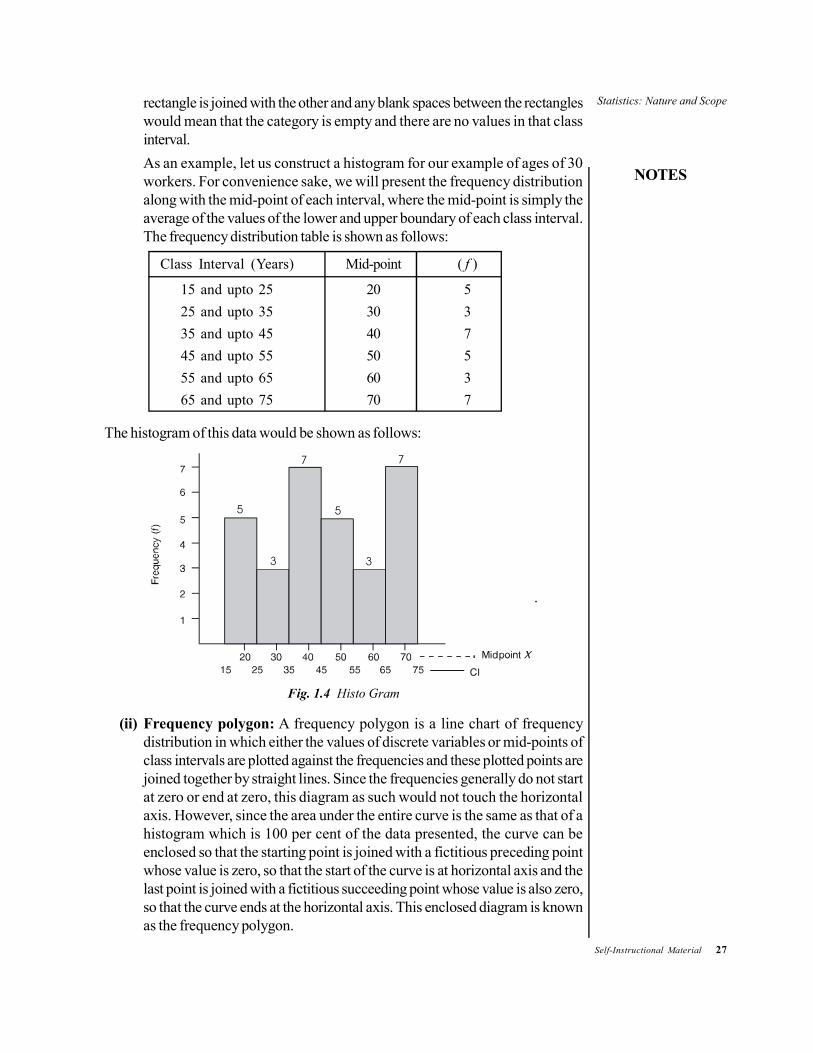
rectangle is joined with the other and any blank spaces between the rectangleswould mean that the category is empty and there are no values in that classinterval.As an example, let us construct a histogram for our example of ages of 30workers. For convenience sake, we will present the frequency distributionalong with the mid-point of each interval, where the mid-point is simply theaverage of the values of the lower and upper boundary of each class interval.The frequency distribution table is shown as follows:
Class Interval (Years) Mid-point ( f )
15 and upto 25 20 525 and upto 35 30 335 and upto 45 40 745 and upto 55 50 555 and upto 65 60 365 and upto 75 70 7
The histogram of this data would be shown as follows:
5
3
7
5
3
7
.
Fig. 1.4 Histo Gram
(ii) Frequency polygon: A frequency polygon is a line chart of frequencydistribution in which either the values of discrete variables or mid-points ofclass intervals are plotted against the frequencies and these plotted points arejoined together by straight lines. Since the frequencies generally do not startat zero or end at zero, this diagram as such would not touch the horizontalaxis. However, since the area under the entire curve is the same as that of ahistogram which is 100 per cent of the data presented, the curve can beenclosed so that the starting point is joined with a fictitious preceding pointwhose value is zero, so that the start of the curve is at horizontal axis and thelast point is joined with a fictitious succeeding point whose value is also zero,so that the curve ends at the horizontal axis. This enclosed diagram is knownas the frequency polygon.

28 Self-Instructional Material
Statistics: Nature and Scope
NOTES
We can construct the frequency polygon from the preceding table as follows:
(20, 5)
(30, 3)
(40, 7)
(50, 5)
(70, 7)
(60, 3)
Fig. 1.5 Frequency Polygon
(iii) Cumulative frequency curve (Ogive): The cumulative frequency curveor ogive is the graphic representation of a cumulative frequency distribution.Ogives are of two types. One of these is less than and the other one isgreater than ogive. Both these ogives are constructed based upon the followingtable of our example of 30 workers.
Class Interval Mid-point ( f ) Cum. Freq. Cum. Freq.(Years) (Less Than) (Greater Than)
15 and upto 25 20 5 5 (less than 25) 30 (more than 15)
25 and upto 35 30 3 8 (less than 35) 25 (more than 25)
35 and upto 45 40 7 15 (less than 45) 22 (more than 35)
45 and upto 55 50 5 20 (less than 55) 15 (more than 45)
55 and upto 65 60 3 23 (less than 65) 10 (more than 55)
65 and upto 75 70 7 30 (less than 75) 7 (more than 65)
Statistics: Nature and Scope
NOTES
Self-Instructional Material 29
(a) Less than Ogive: In this case, less than cumulative frequencies are plottedagainst upper boundaries of their respective class intervals.
Fig. 1.6 Less Than Ogive
(b) Greater than Ogive: In this case, greater than cumulative frequencies areplotted against the lower boundaries of their respective class intervals.
Gre
ater
than
Cum
ulat
ive
Freq
uenc
y
Fig. 1.7 More Than Ogive
These ogives can be used for comparison purposes. Several ogives can be drawnon the same grid, preferably with different colours for easier visualization anddifferentiation.Although, diagrams and graphs are a powerful and effective media for presentingstatistical data, they can only represent a limited amount of information and they arenot of much help when intensive analysis of data is required.

30 Self-Instructional Material
Statistics: Nature and Scope
NOTES
Solved ProblemsProblem 1: Standard tests were administered to 30 students to determine their IQscores. These scores are recorded in the following table.
120 115 118 132 135 125 122 140 137 127
129 130 116 119 132 127 133 126 120 125
130 134 135 127 116 115 125 130 142 140
(a) Arrange this data into an ordered array.
(b) Construct a grouped frequency distribution with suitable class intervals.
(c) Compute for this data:
– Cumulative frequency (<)
– Cumulative frequency (>)
(d) Compute:
– Relative frequency
– Cumulative relative frequency (<)
– Cumulative relative frequency (>)
(e) Construct for this data:
– A histogram
– A frequency polygon
– Cumulative relative ogive (<)
– Cumulative relative ogive (>)
Solution:
(a) The ordered array for this data is as follows:115 115 116 116 118 119 120 120 122 125
125 125 126 127 127 127 129 130 130 132
132 132 133 134 135 135 137 140 140 142

Statistics: Nature and Scope
NOTES
Self-Instructional Material 31
(b) Let there be 6 groupings, so that the size of the class interval be 5. Thefrequency distribution is shown as follows:
Class Interval (CI) Frequency ( f )115 to less than 120 6120 ’’ ’’ ’’ 125 3125 ’’ ’’ ’’ 130 8130 ’’ ’’ ’’ 135 7135 ’’ ’’ ’’ 140 3140 ’’ ’’ ’’ 145 3
(c) The required elements are computed in the following table.
Class Interval ( f ) Cum. Freq.(<) Cum. Freq. (>)
115–120 6 6 (less than 120) 30 (more than 115)120–125 3 9 (less than 125) 24 (more than 120)125–130 8 17 (less than 130) 21 (more than 125)130–135 7 24 (less than 135) 13 (more than 130)135–140 3 27 (less than 140) 6 (more than 135)140–145 3 30 (less than 145) 3 (more than 140)
(d) The computed values of relative frequency, cumulative relative frequency(<) and cumulative relative frequency (>) are shown in the following table:
Class Interval ( f ) Rel. Freq. Cum. Rel. Cum. Rel.Freq. (<) Freq. (>)
115 and upto 120 6 6/30 or 20% 6/30 or 20% (<120) 30/30 or 100% >115)
120 and upto 125 3 3/30 or 10% 9/30 or 30% <125) 24/30 or 80% (>120)
125 and upto 130 8 8/30 or 26.7% 17/30 or 56.7% (<130) 21/30 or 70% (>125)
130 and upto 135 7 7/30 or 23.3% 24/30 or 80% (<135) 13/30 or 43.3% (>130)
135 and upto 140 3 3/30 or 10% 27/30 or 90% (<140) 6/30 or 20% (>135)
140 and upto 145 3 13/30 or 10% 30/30 or 100% (<145) 3/ 30 or 10% (>140)
Total = 30
(e) Before we construct the histogram and other diagrams, let us first determinethe midpoint (X) of each class interval.
Class Interval ( f ) Mid-point (X)
115–120 6 117.5120–125 3 122.5125–130 8 127.5130–135 7 132.5135–140 3 137.5140–145 3 142.5

32 Self-Instructional Material
Statistics: Nature and Scope
NOTES
A histogram
A frequency polygon

Statistics: Nature and Scope
NOTES
Self-Instructional Material 33
A cumulative frequency ogive (<)
A cumulative frequency ogive (>)
Problem 2: Construct a stem and leaf display for the data of IQ scores presentedin the preceding example.
Solution:
The IQ scores of the given 30 students are presented in an ordered array, as follows:115 115 116 116 118 119 120 120 122 125
125 125 126 127 127 127 129 130 130 132
132 132 133 134 135 135 137 140 140 142

34 Self-Instructional Material
Statistics: Nature and Scope
NOTES
The stem would consist of the first two digits and the leaf would consist of the lastdigit.
Stem Leaves
11 5 5 6 6 8 9
12 0 0 2 5 5 5 6 7 7 7 9
13 0 0 2 2 2 3 4 5 5 7
14 0 0 2
Problem 3: Suppose the Office of the Management and Budget (OMB) hasdetermined that the Federal Budget for 2008 would be utilized for proportionatespending in the following categories. Construct a pie chart to represent this data.
Category Per cent AllocationDirect benefit to individuals 40State, local grants 15Military spending 25Debt service 15Misc. operations 5
Total 100%
Solution:
The pie chart is presented as follows. Care must be taken so that the percentageallocation of budget is represented by the appropriate proportion of the pie.
CHECK YOUR PROGRESS
6. What is stem and leaf display?7. What is a pictogram?8. What is a frequency polygon?

Statistics: Nature and Scope
NOTES
Self-Instructional Material 35
1.5 SUMMARY
• In order for the quantitative and numerical data to be identified as statistics, itmust possess certain identifiable characteristics. Some of these characteristicsinclude: (a) Statistics are aggregates of facts (b) Statistics are numericallyexpressed (c) Statistical data is collected in a systematic manner.
• Statistics is no longer confined to the domain of mathematics. It has spread tomost of the branches of knowledge including social sciences and behaviouralsciences. One of the reasons for its phenomenal growth is the variety ofdifferent functions attributed to it.
• The field of statistics, though widely used in all areas of human knowledgeand widely applied in a variety of disciplines such as business, economics andresearch, has its own limitations. Some of the limitations include: (a) It doesnot deal with individual values (b) Statistical conclusions are not universallytrue (c) Statistics can be misused.
• There is hardly any walk of life which has not been affected by statistics—ranging from a simple household to big businesses and the government. Someof the important areas where the knowledge of statistics is usefully appliedare government, economics, physical, natural and social sciences, statisticsand research.
• Statistics influence the operations of business and management in manydimensions. Statistical applications include the area of production, marketing,promotion of product, financing, distribution, accounting, marketing research,manpower planning, forecasting, research and development and so on.
• A researcher needs to be familiar with the various statistical methods so as tobe able to use the appropriate method in his research study. There are certainbasic statistical methods, which can be classified into three groups as follows:(a) Descriptive statistics (b) Inferential statistics (c) Measures of centraltendency and dispersion.
• According to Smith, descriptive statistics is the formulation of rules andprocedures where data can be placed in a useful and significant order. Thefoundation of applicability of descriptive statistics is the need for completedata presentation.
• Statistical data can be organized into a frequency distribution which simplylists the value of the variable and frequency of its occurrence in a tabularform. A frequency distribution can be defined as the list of all the valuesobtained in the data and the corresponding frequency with which these valuesoccur in the data.
• The number of groups and the size of class interval are more or less arbitraryin nature within the general guidelines established for constructing a frequencydistribution.

36 Self-Instructional Material
Statistics: Nature and Scope
NOTES
• In statistics, calculations are performed by arranging the large raw (ungrouped)data set into grouped data and are represented in tabular form called frequencydistribution table. The data to be grouped must be homogenous andcomparable. The frequency distribution table gives the size and the numberof class intervals. The range of each class is defined by the class boundaries.
• The data collected first-hand for any statistical evaluation is considered asraw or ungrouped data as it is not meaningful and does not present a clearpicture. It is then arranged in the ascending or the descending order in atabular form called array.
• While the frequency distribution table tells us the number of units in eachclass interval, it does not tell us directly the total number of units that lie belowor above the specified values of class intervals. This can be determined froma cumulative frequency distribution. When the interest of the investigatorfocusses on the number of items below a specified value, then this specifiedvalue is the upper limit of the class interval. It is known as less than cumulativefrequency distribution.
• Stem and leaf display is another form of presentation of the data distribution.It allows us to condense data but still retain the individuality of the data. Theidea is based on an analogy to plants. The leaves in the stem and leaf diagramare the last digit in each number of observed data. The first digit or digits, asthe case may be, are the stem. All the values in the stem are listed in order ina column and a vertical line is drawn beside them and then all the correspondingleaf values are recorded for each stem in a row to the right of the verticalline.
• The data we collect can often be more easily understood for interpretation ifit is presented graphically or pictorially. Diagrams and graphs give visualindications of magnitudes, groupings, trends and patterns in the data. Theseimportant features are more simply presented in the form of graphs. Also,diagrams facilitate comparisons between two or more sets of data.
• Diagrams are more suitable to illustrate discrete data, while continuous datais better represented by graphs. The following are the diagrammatic andgraphic representation methods that are commonly used.
1.6 KEY TERMS
• Statistics: It is the practice or science of collecting and analysing numericaldata in large quantities, especially for the purpose of inferring proportions in awhole from those in a representative sample.
• Economics: It is a branch of knowledge concerned with the production,consumption, and transfer of wealth.

Statistics: Nature and Scope
NOTES
Self-Instructional Material 37
• Gross National Product (GNP): It is the total value of goods produced andservices provided by a country during one year, equal to the gross domesticproduct plus the net income from foreign investments.
• Frequency distribution: It is a mathematical function showing the numberof instances in which a variable takes each of its possible values.
• Cumulative: It refers to increasing or increased in quantity, degree, or forceby successive additions.
1.7 ANSWERS TO ‘CHECK YOUR PROGRESS’
1. According to Smith, descriptive statistics is the formulation of rules andprocedures where data can be placed in a useful and significant order. Thefoundation of applicability of descriptive statistics is the need for completedata presentation.
2. Hypothesis testing attempts to validate or disprove preconceived ideas. Increating hypothesis, one thinks of a possible explanation for a remarkedbehaviour. The hypothesis dictates the data selected to be analysed for furtherinterpretations.
3. The table must have a title and an identification number. The table title shouldbe short and usually would not include any verbs or articles. It only refers tothe population or parameter being studied. The title should be briefly yetclearly descriptive of the information provided. The numbering of tables isusually in a series and generally one makes use of roman numbers to identifythem.
4. A frequency distribution can be defined as the list of all the values obtained inthe data and the corresponding frequency with which these values occur inthe data.
5. The data collected first-hand for any statistical evaluation is considered asraw or ungrouped data as it is not meaningful and does not present a clearpicture.
6. Stem and leaf display is another form of presentation of the data distribution.It allows us to condense data but still retain the individuality of the data. Theidea is based on an analogy to plants.
7. Pictogram means presentation of data in the form of pictures. It is quite apopular method used by governments and other organizations for informationalexhibitions. Its main advantage is its attractive value. Pictograms stimulateinterest in the information being presented.
8. A frequency polygon is a line chart of frequency distribution in which eitherthe values of discrete variables or mid-points of class intervals are plottedagainst the frequencies and these plotted points are joined together by straightlines.

38 Self-Instructional Material
Statistics: Nature and Scope
NOTES
1.8 QUESTIONS AND EXERCISES
Short-Answer Questions1. ‘Statistics are numerically expressed’. Explain this statement with examples.2. What are the various functions of statistics?3. How is a frequency distribution constructed?4. Discuss Cumulative Frequency Curve (Ogive) with examples.
Long-Answer Questions1. Discuss the limitations of statistics in detail.2. Describe the areas in which statistics have been extensively and effectively
used.3. What are the three different types of graphic representation of statistics?
Discuss in detail.
1.9 FURTHER READING
Garett, H. E. 1971. Statistics in Psychology and Education, 6th Indian Edition.Bombay: Vakils, Feffer and Simon.
Guilford, J. F. 1954. Psychometric Methods, 2nd Edition. New Delhi: TataMcGraw Hill.
Health, R. W. and N. M. Downie. 1970. Basic Statistical Methods, 3rd Edition.New York: Harper International.
McNemar, J. 1967. Psychological Theory. New York: McGraw Hill.

Measures of CentralTendency
NOTES
Self-Instructional Material 39
UNIT 2 MEASURES OF CENTRALTENDENCY
Structure2.0 Introduction2.1 Unit Objectives2.2 Measures of Central Tendency: Calculation, Interpretation and Use of
Measures of Central Tendency2.2.1 Measures of Central Tendency: Arithmetic Mean, Median and Mode2.2.2 Weighted Arithmetic Mean; 2.2.3 Harmonic Mean
2.3 Measures of Variability/Dispersion: When and Where to Use the VariousMeasures of Variability
2.3.1 Quartile Deviation (QD); 2.3.2 Average Deviation (AD)2.3.3 Standard Deviation (SD); 2.3.4 Range (R); 2.3.5 Skewness2.3.6 Kurtosis; 2.3.7 Comparison of Various Measures of Dispersion2.3.8 Coefficient of Variation
2.4 Summary2.5 Key Terms2.6 Answers to ‘Check Your Progress’2.7 Questions and Exercises2.8 Further Reading
2.0 INTRODUCTION
In this unit, you will learn about the measures of central tendency and dispersion.There are several commonly used measures of central tendency, such as arithmeticmean, mode and median. These values are very useful not only in presenting theoverall picture of the entire data but also for the purpose of making comparisonsamong two or more sets of data. In addition, you will learn about the harmonicmean. If a, b, c are in HP (harmonical progression), then b is called a HarmonicMean between a and c, written as HM. Moreover, you will also learn about themeasures of dispersion. A measure of dispersion or simply dispersion may be definedas statistics signifying the extent of the scatteredness of items around a measure ofcentral tendency. Under this, you will study range, quartile deviation, average deviationand standard deviation. Coefficient of variation will also be discussed in this unit.
2.1 UNIT OBJECTIVES
After going through this unit, you will be able to:• Describe the interpretation and uses of measures of central tendency• Discuss the computation of arithmetic mean, median and mode• Explain the concept of measures of variability/dispersion and its significance
in statistical analysis• Discuss range, quartile deviation, average deviation and standard deviation

40 Self-Instructional Material
Measures of CentralTendency
NOTES
2.2 MEASURES OF CENTRAL TENDENCY:CALCULATION, INTERPRETATION AND USEOF MEASURES OF CENTRAL TENDENCY
There are several commonly used measures of central tendency, such as arithmeticmean, mode and median. These values are very useful not only in presenting theoverall picture of the entire data but also for the purpose of making comparisonsamong two or more sets of data.
As an example, questions like ‘How hot is the month of June in Delhi?’ canbe answered, generally by a single figure of the average for that month. Similarly,suppose we want to find out if boys and girls at age 10 years differ in height for thepurpose of making comparisons. Then, by taking the average height of boys of thatage and average height of girls of the same age, we can compare and record thedifferences.
While arithmetic mean is the most commonly used measure of central location,mode and median are more suitable measures under certain set of conditions andfor certain types of data. However, each measure of central tendency should meetthe following requisites:
1. It should be easy to calculate and understand.2. It should be rigidly defined. It should have only one interpretation so
that the personal prejudice or bias of the investigator does not affect itsusefulness.
3. It should be representative of the data. If it is calculated from a sample,then the sample should be random enough to be accurately representingthe population.
4. It should have sampling stability. It should not be affected by samplingfluctuations. This means that if we pick 10 different groups of college studentsat random and compute the average of each group, then we should expectto get approximately the same value from each of these groups.
5. It should not be affected much by extreme values. If few very small orvery large items are present in the data, they will unduly influence thevalue of the average by shifting it to one side or other, so that the averagewould not be really typical of the entire series. Hence, the average chosenshould be such that it is not unduly affected by such extreme values.
2.2.1 Measures of Central Tendency: Arithmetic Mean,Median and Mode
If the progress scores of the students of a class are taken and they are arranged ina frequency distribution, we may sometime find that there are very few studentswho either score very high or very low. The marks of most of the student will liesomewhere between the highest and the lowest scores of the whole class. Thistendency of a group about distribution is named as central tendency and typical

Measures of CentralTendency
NOTES
Self-Instructional Material 41
score that lies in between the extremes and shared by most of the students is referredto as a measure of central tendency. Tate in 1955 defines the measures of centraltendency as, A sort of average or typical value of the items in the series and itsfunction is to summarize the series in terms of this average value.
The most common measures of central tendency are:1. Arithmetic Mean or Mean2. Median3. Mode
Let us consider the three measures of central tendency.(a) Arithmetic Mean: This is also commonly known as simply the mean. Even
though average, in general, means any measure of central location, when weuse the word average in our daily routine, we always mean the arithmeticaverage. The term is widely used by almost every one in daily communication.We speak of an individual being an average student or of average intelligence.We always talk about average family size or average family income or GradePoint Average (GPA) for students, and so on.
Calculating Arithmetic Mean (M): The simplest but most useful measure ofcentral tendency is the arithmetic mean. It can be defined as the sum of all thevalues of the items in a series divided by the number of items. It is represented bythe letter M.
Calculation of Mean in the Case of Ungrouped DataLet X1, X2, X3, X4, X5, X6, X7, X8, X9 and X10 be the scores obtained by 10 students onan achievement test. Then the arithmetic mean or mean score of the group of theseten students can be calculated as:
M = X1 + X2 + X3 + X4 + X5 +…+ X10 /10The formula for calculating the mean of an ungrouped data is as follows:
M = ∑X/NWhere, ∑X stands for the sum of sores or values of the items and N for the
total number in a series or group.
Calculation of Mean in the Case of Grouped Data (Data in the formof Frequency Distribution)General Method: In a frequency distribution where all the frequencies are greaterthan one, the mean is calculated by the formula:
M= ∑ f X / NWhere, X represents the mid-point of the class interval, f its respective
frequency and N the total of all frequencies.Short-Cut Method: Mean for the grouped data can be computed easily with thehelp of following formula:
M = A + ∑ f x′/N × i

42 Self-Instructional Material
Measures of CentralTendency
NOTES
Where,A = Assumed mean.i = Class interval.f = Respective frequency of the mid-values of the class intervals.N = Total Frequency.x′ = X – A / i
Combined Mean: If the arithmetic averages and the number of items in two ormore related groups are known, the combined (or composite) mean of the entiregroup can be obtained by the following formula:
X = 1 1 2 2
1 2
n x n xn n
The advantage of combined arithmetic mean is that, one can determine the overallmean of the combined data without having to going back to the original data.For example:We can find the combined mean for the data given below:
n1 = 10, x1 = 2, n2 = 15, x2 = 3To obtain the mean:
X = 1 1 2 2
1 2
n x n xn n
=10 2 15 3
10 15
=20 45
25= 2.6
For discussion purposes, let us assume a variable X which stands forsome scores, such as the ages of students. Let the ages of 5 students be 19,20, 22, 22 and 17 years. Then variable X would represent these ages asfollows:
X: 19, 20, 22, 22, 17Placing the Greek symbol σ(Sigma) before X would indicate a command thatall values of X are to be added together. Thus:
σX = 19 + 20 + 22 + 22 + 17The mean is computed by adding all the data values and dividing it by the
number of such values. The symbol used for sample average is X so that:
19 20 22 22 175
X

Measures of CentralTendency
NOTES
Self-Instructional Material 43
In general, if there are n values in the sample, then:
1 2 ......... nX X XX
nIn other words,
1 , 1, 2 ... .
n
ii
XX i n
n i = 1, 2, ..., × 2 n.
The above formula states, add up all the values of Xi where the value ofi starts at 1 and ends at n with unit increments so that i = 1, 2, 3, ..., n.If instead of taking a sample, we take the entire population in our calculationsof the mean, then the symbol for the mean of the population is µ (mu) and thesize of the population is N, so that:
1 , 1, 2 ... .
N
ii
Xi N
N
If we have the data in grouped discrete form with frequencies, then thesample mean is given by:
( )f XXf
Where, Σ f = Summation of all frequencies’ n.Σf(X) = Summation of each value of X multiplied by its
corresponding frequency (f).
Example 2.1: Let us take the ages of 10 students as follows:
19, 20, 22, 22, 17, 22, 20, 23, 17, 18Solution: This data can be arranged in a frequency distribution as follows:
(X) (f) f(X) 17 2 34 18 1 18 19 1 19 20 2 40 22 3 66 23 1 23
Total = 10 200 In the above case we have ∑f = 10 and ∑f(X) = 200, so that:
X =( )f Xf
= 200/10 = 20

44 Self-Instructional Material
Measures of CentralTendency
NOTES
Characteristics of the MeanThe arithmetic mean has three interesting properties. These are:
1. The sum of the deviations of individual values of X from the mean will alwaysadd up to zero. This means that if we subtract all the individual values fromtheir mean, then some values will be negative and some will be positive, but ifall these differences are added together then the total sum will be zero. Inother words, the positive deviations must balance the negative deviations. Orsymbolically:
1( )
n
ii
X X = 0, i = 1, 2, ..., n.
2. The second important characteristic of the mean is that it is very sensitive toextreme values. Since the computation of the mean is based upon inclusion ofall values in the data, an extreme value in the data would shift the meantowards it, thus making the mean unrepresentative of the data.
3. The third property of the mean is that the sum of squares of the deviationsabout the mean is minimum. This means that if we take differences betweenindividual values and the mean and square these differences individually andthen add these squared differences, then the final figure will be less than thesum of the squared deviations around any other number other than the mean.Symbolically, it means that:
2
1( )
n
ii
X X = Minimum, i = 1, 2, ..., n.
Advantages of MeanThe following are the various advantages of mean:
1. Its concept is familiar to most people and is intuitively clear.2. Every data set has a mean, which is unique and describes the entire data to
some degree. For instance, when we say that the average salary of a professoris ` 25,000 per month, it gives us a reasonable idea about the salaries ofprofessors.
3. It is a measure that can be easily calculated.4. It includes all values of the data set in its calculation.5. Its value varies very little from sample to sample taken from the same
population.6. It is useful for performing statistical procedures, such as computing and
comparing the means of several data sets.
Disadvantages of MeanThe following are the various disadvantages of mean:
1. It is affected by extreme values, and hence, not very reliable when the dataset has extreme values especially when these extreme values are on one side

Measures of CentralTendency
NOTES
Self-Instructional Material 45
of the ordered data. Thus, a mean of such data is not truly a representative ofsuch data. For instance, the average age of three persons of ages 4, 6 and 80years gives us an average of 30.
2. It is tedious to compute for a large data set as every point in the data set is tobe used in computations.
3. We are unable to compute the mean for a data set that has open-endedclasses either at the high or at the low end of the scale.
4. The mean cannot be calculated for qualitative characteristics, such as beautyor intelligence, unless these can be converted into quantitative figures, suchas intelligence into IQs.
(b) Median: The median is a measure of central tendency and it appears in thecentre of an ordered data. It divides the list of ordered values in the data intotwo equal parts so that half of the data will have values less than the medianand half will have values greater than the median.If the total number of values is odd, then we simply take the middle value asthe median. For instance, if there are 5 numbers arranged in order, such as 2,3, 3, 5, 7, then 3 is the middle number and this will be the median. However, ifthe total number of values in the data is even, then we take the average of themiddle two values. For instance, let there be 6 numbers in the ordered data,such as 2, 3, 3, 5, 7, 8, then the average of middle two numbers which are 3and 5 would be the median, which is:
Median = (3 5) 4
2
In general, the median is 1 th2
n observation in the ordered data.
The median is a useful measure in the sense that it is not unduly affected byextreme values and is specially useful in open ended frequencies.
Calculating Median (Md): If the items of a series are arranged in ascending ordescending order of magnitude, the measure or value of the central item in theseries is termed as median. The median of a distribution can thus be said as the pointon the score scale below which half (or 50 per cent) of the scores fall. Thus, medianis the score or the value of that central item which divides the series into two equalparts. Therefore, it should be understood that the central item itself is not the median.It is only the measure or value of the central item that is known as the median. Forexample, if we arrange in ascending or descending order the marks of 5 students,then the marks obtained by the third student from either side will be termed asmedian of the scores of the group of students under consideration.
Computation of Median for Ungrouped DataThe following two situations could arise:
1. When N (no. of items in a series) is odd: In this case where N is odd (notdivisible by 2), the median can be computed by the following formula:
Md = The measure or value of the (N + 1)/2 th item.

46 Self-Instructional Material
Measures of CentralTendency
NOTES
2. When N (no. of items in a series) is even: In this case where N is even(divisible by 2), the median can be determined by the following formula:Md = The value of the (N/2) th item + The value of [(N/2) + 1] th item/2
Calculation of Median for Grouped Data (In the Form of FrequencyDistribution)If the data is available in the form of a frequency distribution like below, thencalculation of median first requires the location of median class.
Scores f
65-69 160-64 355-59 450-54 745-49 940-44 1135-39 830-34 425-29 220-24 1
N = 50
Actually, median is the measure or score of the central item. Therefore, it isneeded to locate the central item. It may be done through the formulae given earlierin case of ungrouped data for the odd and even values of N (total frequencies).Here, in the present distribution, N (= 50) is even. Therefore, median will fallsomewhere between the score of 25th and 26th items in the given distribution. In thegiven frequency distribution table, if we add frequencies either above or below wemay see that the class interval designated as 40-44 is to be labeled as the classwhere the score representing median will fall.
After estimating the median class, the median of the distribution may beinterpolated with the help of following formula:
Md = L + [ (N/2) – F /f] × iWhere,
L = Exact lower limit of the median class.F = Total of all frequencies before in the median class.f = Frequency of the median class.i = Class interval.N = Total of all the frequency.

Measures of CentralTendency
NOTES
Self-Instructional Material 47
By applying the above formula, we can compute the median of the givendistribution in the following way:
Md = 39.5+ (50/2) –15 / 11× 5 = 39.5 + 10/11 × 5= 39.5 + 50/11 = 39.5 + 4.55 = 44.05
Advantages of MedianThe following are the advantages of median:
1. Median is a positional average and hence the extreme values in the data setdo not affect it as much as they do to the mean.
2. Median is easy to understand and can be calculated from any kind of data,even for grouped data with open-ended classes.
3. We can find the median even when our data set is qualitative and can bearranged in the ascending or the descending order, such as average beauty oraverage intelligence.
4. Similar to mean, median is also unique, meaning that there is only one medianin a given set of data.
5. Median can be located visually when the data is in the form of ordered data.6. The sum of absolute differences of all values in the data set from the median
value is minimum, meaning that it is less than any other value of centraltendency in the data set, which makes it more central in certain situations.
Disadvantages of MedianThe following are the disadvantages of median:
1. The data must be arranged in order to find the median. This can be very timeconsuming for a large number of elements in the data set.
2. The value of the median is affected more by sampling variations. Differentsamples from the same population may give significantly different values ofthe median.
3. The calculation of median in case of grouped data is based on the assumptionthat the values of observations are evenly spaced over the entire class intervaland this is usually not so.
4. Median is comparatively less stable than the mean, particularly for smallsamples, due to fluctuations in sampling.
5. Median is not suitable for further mathematical treatment. For instance, wecannot compute the median of the combined group from the median values ofdifferent groups.
(c) Mode: The mode is another form of average and can be defined as the mostfrequently occurring value in the data. The mode is not affected by extremevalues in the data and can easily be obtained from an ordered set of data. Itcan be useful and more representative of the data under certain conditionsand is the only measure of central tendency that can be used for qualitativedata. For instance, when a researcher quotes the opinion of an average person,

48 Self-Instructional Material
Measures of CentralTendency
NOTES
he is probably referring to the most frequently expressed opinion which is themodal opinion. In our example of ages of 10 students as:
19, 20, 22, 22, 17, 22, 20, 23, 17 and 18The mode is 22, since it occurs more often than any other value in this data.
Calculating Mode (M0): Mode is defined as the size of a variable which occursmost frequently. It is the point on the score sale that corresponds to the maximumfrequency of the distribution. In any series, it is the value of the item which is mostcharacteristics or common and is usually repeated the maximum number of times.
Computation of Mode for Ungrouped DataMode can easily be computed merely by looking at the data. All that one has to do isto find out the score which is repeated maximum number of times.
For example, suppose we have to find out the value of mode from the followingscores of students:
25, 29, 24, 25, 27, 25, 28, 25, 29Here, the score 25 is repeated maximum number of times and thus, value of
the mode in this case is 25.
Computation of Mode for Grouped DataWhen data is available in the form of frequency distribution, the mode is computedfrom the following formula:
Mode (M0) = 3 Md – 2MWhere, Md is the median and M is the mean of the given distribution. The
mean as well as the median of the distribution are first computed and then, with thehelp of the above formula, mode is computed.
Another Method for Grouped DataMode can be computed directly from the frequency distribution table withoutcalculating mean and median. For this purpose, we can use the following formula:
M0 = L + f1/ (f1 + f–1 ) × iWhere,
L = Lower limit of the model class (the class in which mode maybe supposedto lie).
i = Class interval.f 1 = Frequency of the class adjacent to the modal class for which lower
limit is greater than that for the modal class.f–1= Frequency of the class adjacent to the modal class for which the lower
limit is less than that for the modal class.
Advantages of ModeThe following are the advantages of mode:
1. Similar to median, the mode is not affected by extreme values in the data.

Measures of CentralTendency
NOTES
Self-Instructional Material 49
2. Its value can be obtained in open-ended distributions without ascertaining theclass limits.
3. It can be easily used to describe qualitative phenomenon. For instance, ifmost people prefer a certain brand of tea then this will become the modalpoint.
4. Mode is easy to calculate and understand. In some cases it can be locatedsimply by observation or inspection.
Disadvantages of ModeThe following are the disadvantages of mode:
1. Quite often, there is no modal value.2. It can be bi-modal or multi-modal or it can have all modal values making its
significance more difficult to measure.3. If there is more than one modal value, the data is difficult to interpret.4. A mode is not suitable for algebraic manipulations.5. Since the mode is the value of maximum frequency in the data set, it cannot
be rigidly defined if such frequency occurs at the beginning or at the end ofthe distribution.
6. It does not include all observations in the data set, and hence, less reliable inmost of the situations.
2.2.2 Weighted Arithmetic MeanIn the computation of arithmetic mean we had given equal importance to eachobservation in the series. This equal importance may be misleading if the individualvalues constituting the series have different importance as in the following example:
The Raja Toy shop sellsToy Cars at ` 3 eachToy Locomotives at ` 5 eachToy Aeroplanes at ` 7 eachToy Double Decker at ` 9 each
What shall be the average price of the toys sold, if the shop sells 4 toys, one of eachkind?
Mean Price, i.e., x = x∑4
= 244
` = ` 6
In this case the importance of each observation (Price quotation) is equal in asmuch as one toy of each variety has been sold. In the above computation of thearithmetic mean this fact has been taken care of by including ‘once only’ the priceof each toy.
But if the shop sells 100 toys: 50 cars, 25 locomotives, 15 aeroplanes and 10double deckers, the importance of the four price quotations to the dealer is notequal as a source of earning revenue. In fact their respective importance is equal tothe number of units of each toy sold, i.e.,
The importance of Toy Car 50The importance of Locomotive 25

50 Self-Instructional Material
Measures of CentralTendency
NOTES
The importance of Aeroplane 15The importance of Double Decker 10It may be noted that 50, 25, 15, 10 are the quantities of the various classes of
toys sold. It is for these quantities that the term ‘weights’ is used in statistical language.Weight is represented by symbol ‘w’, and Σw represents the sum of weights.
While determining the ‘average price of toy sold’ these weights are of greatimportance and are taken into account in the manner illustrated below:
x = 1 1 2 2 3 3 4 4
1 2 3 4
w x w x w x w xw w w w
= wxw
∑∑
When w1, w2, w3, w4 are the respective weights of x1, x2, x3, x4 which in turnrepresent the price of four varieties of toys, viz., car, locomotive, aeroplane anddouble decker, respectively.
x = (50 3) (25 5) (15 7) (10 9)50 25 15 10
= (150) (125) (105) (90)100
= 470100
= ` 4.70
The table below summarizes the steps taken in the computation of the weightedarithmetic mean.
Σw = 100; Σwx = 470
x = wxw
∑∑
= 470100
= 4.70
The weighted arithmetic mean is particularly useful where we have to computethe mean of means. If we are given two arithmetic means, one for each of twodifferent series, in respect of the same variable, and are required to find the arithmeticmean of the combined series, the weighted arithmetic mean is the only suitablemethod of its determination.
Weighted Arithmetic Mean of Toys Sold by the Raja Toy Shop
Toys Price Per Toy Number Sold Price × Weight` x w xw
Car 3 50 150Locomotive 5 25 125Aeroplane 7 15 105Double Decker 9 10 90
Σw = 100 Σxw = 470
Example 2.2: The arithmetic mean of daily wages of two manufacturing concernsA Ltd. and B Ltd. is 5 and 7, respectively. Determine the average daily wagesof both concerns if the number of workers employed were 2,000 and 4,000,respectively.Solution: (a) Multiply each average (viz., 5 and 7) by the number of workers in theconcern it represents.
(b) Add up the two products obtained in (a) above.(c) Divide the total obtained in (b) by the total number of workers.

Measures of CentralTendency
NOTES
Self-Instructional Material 51
Weighted Mean of Mean Wages of A Ltd. and B Ltd.
Manufacturing Mean Wages Workers Mean Wages ×Concern x Employed Workers Employed
w wx
A Ltd. 5 2,000 10,000B Ltd. 7 4,000 28,000
w∑ = 6,000 wx∑ = 38,000
x = wxw
= 38,0006,000
= ` 6.33
The above mentioned examples explain that ‘Arithmetic Means and Percentage’are not original data. They are derived figures and their importance is relative to theoriginal data from which they are obtained. This relative importance must be takeninto account by weighting while averaging them (means and percentage).
2.2.3 Harmonic MeanIf a, b, c are in HP, then b is called a Harmonic Mean between a and c, written asHM.
Harmonical ProgressionNon zero quantities whose reciprocals are in AP, or Arithmetic Progression aresaid to be in Harmonical Progression, written as HP.Consider the following examples:
(a) 1 1 11, , , , ... ...
3 5 7
(b) 1 1 1 1, , , , ... ...
2 5 8 11
(c) 5 102, , , ...
2 3
(d)1 1 1
, , , ... ... , 02
a ba a b a b
(e) 55 555, , , 11, ... ...
9 7It can be easily checked that in each case, the series obtained by taking
reciprocal of each of the term is an AP.
To Insert n Harmonic Means between a and bLet H1, H2, H3, ..., Hn be the required Harmonic Means. Then,a, H1, H2, ..., Hn, b are in HP
i.e.,1 2
1 1 1 1 1, , , ..., ,na H H H b are in AP

52 Self-Instructional Material
Measures of CentralTendency
NOTES
Then, 1b
= (n + 2)th term of an AP
= 1a
+ (n + 1)dWhere d is the common difference of AP.
This gives, d = ( 1)
a bn ab
Now,1
1H
= 1 1( 1)
a bda a n ab
= ( 1) ( 1)
nb b a b a nbn ab n ab
So,1
1H
= ( 1)
a nbn ab
⇒ H1 = ( 1)n ab
a nb
Again,2
1H
= 1 1 2 ( )2( 1)
a bda a n ab
= 2 2 2( 1) ( 1)
nb b a b a b nbn ab n ab
⇒ H2 = ( 1)2
n aba b nb
Similarly,3
1H
= 1 3 23( 1)a b nbd
a n ab
⇒ H3 = ( 1)3 2
n aba b nb
and so on,
1
nH= 1 1 ( )
( 1)n a bnd
a a n ab
= ( 1)
nb b na nbn ab
= ( 1)
na bn ab
⇒ Hn = ( 1)n abna b
Example 2.3: Find the 5th term of 2, 2 12 , 3 1
3 , ... ...
Solution: Let 5th term be x. Then, 1x is 5th term of corresponding AP 1 2 3, , , ... ...
2 5 10
Then, 1x
= 1 2 1 1 14 42 5 2 2 10
⇒1x =
1 2 12 5 10 ⇒ x = 10
Example 2.4: Insert two harmonic means between 1 4and .
2 17

Measures of CentralTendency
NOTES
Self-Instructional Material 53
Solution: Let H1, H2 be two harmonic means between 1 4and
2 17.
Thus, 2, 1 2
1 1 17, ,
4H H are in AP. Let d be their common difference.
Then, 174
= 2 + 3d
⇒ 3d = 94
⇒ d = 34
Thus,1
1H
= 2 + 3 114 4 ⇒ H1 = 4
11
2
1H
= 2 + 2 × 3 74 2 ⇒ H2 = 2
7
Required harmonic means are 4 2,
11 7.
CHECK YOUR PROGRESS
1. Define median.2. In a frequency list, where all the frequencies are greater than one, the
mean is calculated by which formula?3. Give any two disadvantages of mean.
2.3 MEASURES OF VARIABILITY/DISPERSION:WHEN AND WHERE TO USE THE VARIOUSMEASURES OF VARIABILITY
A measure of dispersion or simply dispersion may be defined as statistics signifyingthe extent of the scatteredness of items around a measure of central tendency.
A measure of dispersion may be expressed in an ‘absolute form’ or in a‘relative form’. It is said to be in an absolute form when it states the actual amountby which the value of an item on an average deviates from a measure of centraltendency. Absolute measures are expressed in concrete units, i.e., units in terms ofwhich the data have been expressed, e.g., rupees, centimetres, kilograms, etc., andare used to describe frequency distribution.
A relative measure of dispersion computed is a quotient obtained by dividing theabsolute measures by a quantity in respect to which absolute deviation has beencomputed. It is as such a pure number and is usually expressed in a percentage form.Relative measures are used for making comparisons between two or more distributions.
A measure of dispersion should possess all those characteristics which areconsidered essential for a measure of central tendency, which are as follows:
• It should be based on all observations.• It should be readily comprehensible.
54 Self-Instructional Material
Measures of CentralTendency
NOTES
• It should be fairly easily calculated.• It should be affected as little as possible by fluctuations of sampling.• It should be amenable to algebraic treatment.
Types of Measures of DispersionThere are four measures of dispersion which are given below:
(a) Range (R)(b) Quartile Deviation (QD)(c) Average Deviation (AD)(d) Standard Deviation (SD)
Each of the above measures of dispersion tells us how the individual scoresare scattered or spread throughout the distribution or the given data.
2.3.1 Quartile Deviation (QD)There are many types of measures of dispersion, one of this is the semi-interquartilerange, usually termed as ‘Quartile Deviation’ or QD. Quartiles are the points whichdivide the array into four equal parts. More precisely, Q1 gives the value of the item1/4th the way up the distribution and Q3 the value of the item 3/4th the way up thedistribution. Between Q1 and Q3 are included half the total number of items. Thedifference between Q1 and Q3 includes only the central items but excludes theextremes. Since under most circumstances, the central half of the series tends to befairly typical of all the items, the interquartile range (Q3– Q1) affords a convenientand often a good indicator of the absolute variability. The larger the interquartilerange, the larger the variability.
Usually, one-half of the difference between Q3 and Q1 is used and it is giventhe name of quartile deviation or semi-interquartile range. The interquartile range isdivided by 2 for the reason that half of the interquartile range will, in a normaldistribution, be equal to the difference between the median and any quartile. Thismeans that 50 per cent items of a normal distribution will lie within the intervaldefined by the median plus and minus the semi-interquartile range.
Symbolically,
Q.D. = Q Q3 12−
Where, Q1 and Q3 represent the 1st and 3rd quartiles of dispersion underconsideration. The value Q3 – Q1 is the difference or range between the 3rd and 1stquartiles and is the interquartile range.
For computing quartile deviation, this interquartile range is divided by 2 and,therefore, quartile deviation is also names as semi-interquartile range. In this way,for computing Q, the value of Q1 and Q3 are first determined by the method andthen applying the above formula, we get the value of the quartile deviation.
Let us find quartile deviations for the weekly earnings of labour in the fourworkshops whose data is given in Table 2.1. The computations are as shown inTable 2.1.

Measures of CentralTendency
NOTES
Self-Instructional Material 55
Table 2.1 Weekly Earnings of Labourers in Four Workshops of the Same Type
Weekly EarningsNo. of Workers
` Workshop A Workshop B Workshop C Workshop D
15–16 ... ... 2 ...
17–18 ... 2 4 ...
19–20 ... 4 4 4
21–22 10 10 10 14
23–24 22 14 16 16
25–26 20 18 14 16
27–28 14 16 12 12
29–30 14 10 6 12
31–32 ... 6 6 4
33–34 ... ... 2 2
35–36 ... ... ... ...
37–38 ... ... 4 ...
Total 80 80 80 80
Mean 25.5 25.5 25.5 25.5
The range is as follows:Workshop Range
A 9B 15C 23
D 15
As shown in Table 2.2, Q.D. of workshop A is 2.12 and median value in 25.3.This means that if the distribution is symmetrical, the number of workers whose wagesvary between (25.3–2.1) = 23.2 and (25.3 + 2.1) = 27.4, shall be just half of thetotal cases. The other half of the workers will be more than 2.1 removed from themedian wage. As this distribution is not symmetrical, the distance between Q1 and themedian Q2 is not the same as between Q3 and the median. Hence, the interval definedby median plus and minus semi inter-quartile range will not be exactly the same asgiven by the value of the two quartiles. Under such conditions the range between` 23.2 and 27.4 will not include precisely 50 per cent of the workers.
If quartile deviation is to be used for comparing the variability of any twoseries, it is necessary to convert the absolute measure to a coefficient of quartiledeviation. To do this the absolute measure is divided by the average size of the twoquartiles.
Symbolically,
Coefficient of quartile deviation = Q QQ Q
3 1
3 1
−+

56 Self-Instructional Material
Measures of CentralTendency
NOTES
Applying this to our illustration of four workshops in Table 2.1 the coefficients ofQ.D. are as given in Table 2.2.
Table 2.2 Calculation of Quartile Deviation
Workshop Workshop Workshop WorkshopA B C D
Location of Q2 2N 80 40
2=
80 402
=80 402
=80 402
=
Q224.5 + 40
22−
×30 2 40 3024.5 2
18−
+ × 24.5 +40
16−
×30
2 24.5 +40
16−
×30
2
= 24.5 + 0.9 = 24.5 + 1.1 = 24.5 + 0.75 = 24.5 + 0.75= 25.4 = 25.61 = 25.25 = 25.25
Location of Q1 4N 80 20
4=
80 204
=80 204
=80 204
=
Q120 1022.5 2
22−
+ ×20 1622.5 2
14−
+ ×20 1020.5 2
10−
+ ×20 1822.5 2
16−
+ ×
= 22.5 + .91 = 22.5 + .57 = 20.5 + 2 = 22.5 + .25= 23.41 = 23.07 = 22.5 = 22.75
Location of Q334N 803 60
4× = 60 60 60
Q360 5226.5 2
14−
+ ×60 4826.5 2
16−
+ ×60 5026.5 2
12−
+ ×60 5026.5 2
12−
+ ×
= 26.5 + 1.14 = 26.5 + 1.5 = 26.5 + 1.67 = 26.5 + 1.67= 27.64 = 28.0 = 28.17 = 28.17
Quartile Deviation 3 12
Q Q− 27.64 23.412− 28 23.07
2− 28.17 22.5
2− 28 17 22 75
2. .−
= 4.23
2 = ` 2.12 = 4.93
2 = ` 2.46 = 5.67
2 = ` 2.83 = 5.42
2 = `. 2.71
Coefficient of Quartile
Deviation = 27 64 23 4127 64 23 41
. .
. .−+
28 23 0728 23 07
−+
.
.28 17 22 528 17 22 5
. .
. .−+
28 17 22 7528 17 22 75
. .
. .−+
Q QQ Q
3 1
3 1
−+ = 0.083 = 0.097 = 0.112 = 0.106
Characteristics of Quartile DeviationThe following are the characteristics of quartile deviation:
(a) The size of the quartile deviation gives an indication about the uniformity orotherwise of the size of the items of a distribution. If the quartile deviation issmall, it denotes large uniformity. Thus, a coefficient of quartile deviationmay be used for comparing uniformity or variation in different distributions.
(b) Quartile deviation is not a measure of dispersion in the sense that it does notshow the scatter around an average, but only a distance on scale. Consequently,quartile deviation is regarded as a measure of partition.
(c) It can be computed when the distribution has open-end classes.

Measures of CentralTendency
NOTES
Self-Instructional Material 57
Limitations of Quartile DeviationExcept for the fact that its computation is simple and it is easy to understand, aquartile deviation does not satisfy any other test of a good measure of variation.
2.3.2 Average Deviation (AD)
In this section you will study that a weakness of the measures of dispersion, basedupon the range or a portion thereof, is that the precise size of most of the variantshas no effect on the result. As an illustration, the quartile deviation will be the samewhether the variates between Q1 and Q3 are concentrated just above Q1 or they arespread uniformly from Q1 to Q3. This is an important defect from the viewpoint ofmeasuring the divergence of the distribution from its typical value. The AverageDeviation (AD) is employed to answer the objection.
Average Deviation (AD), also called mean deviation, of a frequency distributionis the mean of the absolute values of the deviation from some measure of centraltendency. In other words, mean deviation is the arithmetic average of the variations(deviations) of the individual items of the series from a measure of their centraltendency.
Garrett in 1971 defines Average Deviation (AD) as the mean of deviations ofall the separate scores in the series taken from their mean (occasionally from themedian or mode). It is the simplest measure of variability that takes into account thefluctuation or variation of all the items in a series.
Computation of Average Deviation from Ungrouped DataIn the case of ungrouped data, the average deviation is calculated by the formula
AD = ∑ |x| / NWhere, x = X – M = Deviation of the raw score from the mean of the series
and |x| signifies that in the deviation values we ignore the algebraic signs +ve or –ve.
Computation of Average Deviation from Grouped DataFrom the grouped data, AD can be computed by the following formula:
AD = ∑ |fx| / NWe can measure the deviations from any measure of central tendency, but
the most commonly employed ones are the median and the mean. The median ispreferred because it has the important property that the average deviation from it isthe least.Calculation of mean deviation then involves the following steps:
(a) Calculate the median (or the mean) Md (or X ).(b) Record the deviations | d | = | x – Md | of each of the items, ignoring the
sign.(c) Find the average value of deviations.
Mean Deviation = | |dN
∑

58 Self-Instructional Material
Measures of CentralTendency
NOTES
Example 2.5 explains it better.Example 2.5: Calculate the mean deviation from the following data giving marksobtained by 11 students in a class test.
14, 15, 23, 20, 10, 30, 19, 18, 16, 25, 12.
Solution:
Median = Size of 11 + 12
th item
= Size of 6th item = 18.
Serial No. Marks | x – Median || d |
1 10 82 12 63 14 44 15 35 16 26 18 07 19 18 20 29 23 5
10 25 711 30 12
| |d∑ = 50
Mean deviation from median = | |dN
∑
= 5011
= 4.5 marks
For grouped data, it is easy to see that the mean deviation is given by:
Mean deviation = f df| |∑
∑
Where,| d | = | x – Median | for grouped discrete data.| d | = | M – Median | for grouped continuous data with M as the mid-value of
a particular group.
Examples 2.6 and 2.7 illustrate the use of this formula.Example 2.6: Calculate the mean deviation from the following data:
Size of Item 6 7 8 9 10 11 12Frequency 3 6 9 13 8 5 4

Measures of CentralTendency
NOTES
Self-Instructional Material 59
Solution:
Size Frequency Cumulative Deviations f | d |(f) Frequency from Median
(9) | d |
6 3 3 3 9
7 6 9 2 12
8 9 18 1 9
9 13 31 0 0
10 8 39 1 8
11 5 44 2 10
12 4 48 3 12
48 60
Median = The size of 48 12+ = 24.5th item which is 9.
Therefore, deviations d are calculated from 9, i.e., | d | = | x – 9 |.
Mean deviation = f d
f| |∑
∑ = 6048
= 1.25
Example 2.7: Calculate the mean deviation from the following data:
x 0–10 10–20 20–30 30–40 40–50 50–60 60–70 70–80
f 18 16 15 12 10 5 2 2
Solution:This is a frequency distribution with continuous variable. Thus, deviations arecalculated from mid-values.
x Mid-Value (f) Less than Deviation f | d |(c.f.) from Median
| d |
0–10 5 18 18 19 34210–20 15 16 34 9 14420–30 25 15 49 1 1530–40 35 12 61 11 13240–50 45 10 71 21 21050–60 55 5 76 31 15560–70 65 2 78 41 8270–80 75 2 80 51 102
80 1182

60 Self-Instructional Material
Measures of CentralTendency
NOTES
Median = The size of 802
th item
= 20 615
10+ × = 24
and then, mean deviation = f d
f| |∑
∑
= 118280
= 14.775.
Merits and Demerits of the Average (Mean) DeviationMeritsThe merits are as follows:
1. It is easy to understand.2. As compared to standard deviation, its computation is simple.3. As compared to standard deviation, it is less affected by extreme values.4. Since it is based on all values in the distribution, it is better than range or
quartile deviation.DemeritsThe demerits are as follows:
1. It lacks those algebraic properties which would facilitate its computationand establish its relation to other measures.
2. Due to this, it is not suitable for further mathematical processing.
Coefficient of Mean or Average DeviationThe coefficient or relative dispersion is found by dividing the mean deviations recorded.Thus,
Coefficient of MD = Mean DeviationMean(when deviations were recorded from the mean)
= Mean Deviation
Median
(when deviations were recorded from the median)Applying the above formula to Example 2.7.
Coefficient of MD = 14.77524
= 0.616
2.3.3 Standard Deviation (SD)
By far the most universally used and the most useful measure of dispersion is theStandard Deviation (SD) or root mean square deviation about the mean. We have

Measures of CentralTendency
NOTES
Self-Instructional Material 61
seen that all the methods of measuring dispersion so far discussed are not universallyadopted for want of adequacy and accuracy. The range is not satisfactory as itsmagnitude is determined by most extreme cases in the entire group. Further, therange is notable because it is dependent on the item whose size is largely a matterof chance. Mean deviation method is also an unsatisfactory measure of scatter, as itignores the algebraic signs of deviation. We desire a measure of scatter which isfree from these shortcomings. To some extent standard deviation is one such measure.
The calculation of standard deviation differs in the following respects fromthat of mean deviation. First, in calculating standard deviation, the deviations aresquared. This is done so as to get rid of negative signs without committing algebraicviolence. Further, the squaring of deviations provides added weight to the extremeitems, a desirable feature for certain types of series.
Second, the deviations are always recorded from the arithmetic mean, becausealthough the sum of deviations is the minimum from the median, the sum of squaresof deviations is minimum when deviations are measured from the arithmetic average.The deviation from x is represented by σ.
Thus, standard deviation, σ (sigma) is defined as the square root of the meanof the squares of the deviations of individual items from their arithmetic mean.
Standard deviation of a set of scores is defined as the square root of theaverage of the squares of the deviations of each score from the mean. Symbolically,we can say that:
SD = √ ∑ ( X – M)2/2= √ ∑ x2/ N
Where,X = Individual score.M = Mean of the given set of scores.N = Total number of the sores.x =Derivation of each score from the mean.Standard Deviation or SD is regarded as the most stable and reliable measure
of variability as it employs the mean for its computation. It is often called root meansquare deviation and is denoted by the Greek letter sigma (σ).
Computation of Standard Deviation (SD) from Ungrouped DataStandard deviation can be computed from the ungrouped scores by the formula:
σ = √ ∑ x2 / N
Computation of Standard Deviation (SD) from Grouped DataStandard deviation in case of grouped data can be computed by the formula:
σ = √ ∑ fx2 / N

62 Self-Instructional Material
Measures of CentralTendency
NOTES
Computation of Standard Deviation (SD) from Grouped Data byShort-Cut MethodStandard deviation from grouped data can be computed by the following formula:
σ = √ ∑ fx′ 2 / N − ( ∑ fx′ /N)2
Example 2.8: Compute the standard deviation for the following data:11, 12, 13, 14, 15, 16, 17, 18, 19, 20, 21.
Solution:We first calculate the mean as x = x N/∑ = 176/11 = 16, and then calculate thedeviation as follows:
x (x – x ) (x – x )2
11 –5 2512 –4 1613 –3 914 –2 415 –1 116 0 017 +1 118 +2 419 +3 920 +4 1621 +5 25176 110
Thus,
σ = 11011
10= = 3.16
Example 2.9: Find the standard deviation of the data in the following distributions:
x 12 13 14 15 16 17 18 20f 4 11 32 21 15 8 6 4
Solution:
Since for calculation of x , we need fx∑ and then for σ we need f x x( )−∑ 2 , thecalculations are conveniently made in the following format.
x f fx d = x – x d2 fd2
12 4 48 –3 9 3613 11 143 –2 4 4414 32 448 –1 1 3215 21 315 0 0 016 15 240 1 1 1517 8 136 2 4 3218 5 90 3 9 4520 4 80 5 25 100
∑f =100 ∑fx=1500 ∑fd2=304

Measures of CentralTendency
NOTES
Self-Instructional Material 63
Here, x = /fx f = 1500/100 = 15
and σ = fdf
2∑∑
= 304100 = 3 04. = 1.74
Example 2.10: Compute the standard deviation by the short-cut method for thefollowing data:
11, 12, 13, 14, 15, 16, 17, 18, 19, 20, 21
Solution: Let us assume that A = 15.
x' = (x – 15) x'2
11 –4 16
12 –3 913 –2 414 –1 115 0 016 1 117 2 418 3 919 4 1620 5 2521 6 36
N = 11 ′∑ x = 11 ′∑ x 2 = 121
σ = ′∑ −′∑F
HGIKJ
xN
xN
2 2
= 12111
1111
2− F
HGIKJ
= 11 1−
= 10= 3.16
Another MethodIf we assume A as zero, then the deviation of each item from the assumed mean isthe same as the value of item itself. Thus, 11 deviates from the assumed mean ofzero by 11, 12 deviates by 12, and so on. As such, we work with deviations withouthaving to compute them, and the formula takes the following shape:

64 Self-Instructional Material
Measures of CentralTendency
NOTES
x x2
11 12112 14413 16914 19615 22516 25617 28918 32419 36120 40021 441
176 2,926
σ = xN
xN
2 2∑ − ∑F
HGIKJ
= 2 − FHG
IKJ
92611
17611
2 = 266 256− = 3.16
Combining Standard Deviations of Two DistributionsIf we were given two sets of data of N1 and N2 items with means x1 and x2 andstandard deviations σ1 and σ2, respectively, we can obtain the mean and standarddeviation x and σ of the combined distribution by the following formulae:
x = N x N xN N
1 1 2 2
1 2
++
and σ = N N N x x N x x
N N1 1
22 2
21 1
22 2
2
1 2
σ σ+ + − + −
+
( ) ( )
Example 2.11: The mean and standard deviations of two distributions of 100 and150 items are 50, 5 and 40, 6, respectively. Find the standard deviation of all takentogether.Solution:
Combined mean,
x = N x N xN N
1 1 2 2
1 2
++
= 100 50 150 40100 150× ×+
+
= 44Combined standard deviation,
σ = 2 2 2 2
1 1 2 2 1 1 2 2
1 2
( ) ( )N N N x x N x xN N

Measures of CentralTendency
NOTES
Self-Instructional Material 65
= 100 5 150 6 100 44 50 150 44 40100 150
2 2 2 2× ( ) ( ) ( ) ( )+ + − + −+
= 7.46.Example 2.12: A distribution consists of three components with 200, 250, 300items having mean 25, 10 and 15 and standard deviation 3, 4 and 5, respectively.Find the standard deviation of the combined distribution.Solution:In the usual notations, we are given here
N1 = 200, N2= 250, N3 = 300x1 = 25, x2 = 10, x3 = 15
For the combination of three series the formula will be:
x = N x N x N xN N N
1 1 2 2 3 3
1 2 3
+ ++ +
= 200 25 250 10 300 15200 250 300
× × ×+ ++ +
= 12000750
= 16
and,
σ =
2 2 2 21 1 2 2 3 3 1 1
2 22 2 3 3
1 2 3
( )
( ) ( )
N N N N x x
N x x N x xN N N
= 200 9 250 16 300 25 200 81 250 36 300 1200 250 300
× × × × × ×+ + + + ++ +
= 51 73 7 19. .=
2.3.4 Range (R)
Range (R) of a set of data is the difference between the largest and smallest values.It is the simplest measure of variability or dispersion and is calculated by subtractingthe lowest score in the series from the highest. But it is very rough measure of thevariability of series. It takes only extreme scores into consideration and ignores thevariation of individual items.
Thus, the crudest measure of dispersion is the range of the distribution. Therange of any series is the difference between the highest and the lowest values inthe series. If the marks received in an examination taken by 248 students are arrangedin ascending order, then the range will be equal to the difference between the highestand the lowest marks.
In a frequency distribution, the range is taken to be the difference betweenthe lower limit of the class at the lower extreme of the distribution and the upperlimit of the class at the upper extreme.

66 Self-Instructional Material
Measures of CentralTendency
NOTES
Consider the data on weekly earnings of worker on four workshops given inTable 2.1.
From these figure in Table 2.1, it is clear that the greater the range, thegreater is the variation of the values in the group.
The range is a measure of absolute dispersion and as such cannot be usefullyemployed for comparing the variability of two distributions expressed in differentunits. The amount of dispersion measured, say, in pounds, is not comparable withdispersion measured in inches. Thus, the need of measuring relative dispersion arises.
An absolute measure can be converted into a relative measure if we divide itby some other value regarded as standard for the purpose. We may use the mean ofthe distribution or any other positional average as the standard.For Table 2.1, the relative dispersion would be,
Workshop A = 925 5.
Workshop C = 2325 5.
Workshop B = 1525 5.
Workshop D = 1525 5.
An alternate method of converting an absolute variation into a relative onewould be to use the total of the extremes as the standard. This will be equal todividing the difference of the extreme items by the total of the extreme items. Thus,
Relative Dispersion = Difference of extreme items, i.e, Range
Sum of extreme items
The relative dispersion of the series is called the coefficient or ratio ofdispersion. In our example of weekly earnings of workers considered earlier, thecoefficients would be,
Workshop A = 921 30
951+
= Workshop B = 1517 32
1549+
=
Workshop C = 2315 38
2353+
= Workshop D= 1519 34
1553+
=
Merits and Limitations of RangeMeritsOf the various characteristics that a good measure of dispersion should possess, therange has only two, which are as follows:
1. It is easy to understand.2. Its computation is simple.
LimitationsBesides the aforesaid two qualities, the range does not satisfy the other test of agood measure and hence it is often termed as a crude measure of dispersion.The following are the limitations that are inherent in the range as a concept ofvariability:

Measures of CentralTendency
NOTES
Self-Instructional Material 67
1. Since it is based upon two extreme cases in the entire distribution, the rangemay be considerably changed if either of the extreme cases happens to dropout, while the removal of any other case would not affect it at all.
2. It does not tell anything about the distribution of values in the series relativeto a measure of central tendency.
3. It cannot be computed when distribution has open-end classes.4. It does not take into account the entire data. These can be illustrated by the
following illustration. Consider the data given in Table 2.3.Table 2.3 Distribution with the Same Number of Cases,
but Different Variability
No. of StudentsClass
Section Section SectionA B C
0–10 ... ... ...10–20 1 ... ...20–30 12 12 1930–40 17 20 1840–50 29 35 1650–60 18 25 1860–70 16 10 1870–80 6 8 2180–90 11 ... ...90–100 ... ... ...
Total 110 110 110
Range 80 60 60
The table is designed to illustrate three distributions with the same number ofcases but different variability. The removal of two extreme students from Section Awould make its range equal to that of B or C.
The greater range of A is not a description of the entire group of 110 students,but of the two most extreme students only. Further, though sections B and C havethe same range, the students in Section B cluster more closely around the centraltendency of the group than they do in Section C. Thus, the range fails to reveal thegreater homogeneity of B or the greater dispersion of C. Due to this defect, it isseldom used as a measure of dispersion.
Specific Uses of RangeIn spite of the numerous limitations of the range as a measure of dispersion, it is themost appropriate under the following circumstances:
(a) In situations where the extremes involve some hazard for which preparationshould be made, it may be more important to know the most extreme cases tobe encountered than to know anything else about the distribution. For example,an explorer, would like to know the lowest and the highest temperatures on

68 Self-Instructional Material
Measures of CentralTendency
NOTES
record in the region he is about to enter; or an engineer would like to knowthe maximum rainfall during 24 hours for the construction of a storm waterdrain.
(b) In the study of prices of securities, range has a special field of activity. Thus,to highlight fluctuations in the prices of shares or bullion, it is a commonpractice to indicate the range over which the prices have moved during acertain period of time. This information, besides being of use to the operators,gives an indication of the stability of the bullion market, or that of the investmentclimate.
(c) In statistical quality control, range is used as a measure of variation. We, forexample, determine the range over which variations in quality are due torandom causes, which is made the basis for the fixation of control limits.
2.3.5 Skewness
Skewness refers to lack of symmetry in a distribution. In a symmetrical distribution,the mean, median and mode coincide. Positive and negative skewness is shown inFigure 2.1.
Fig. 2.1 Skewness
In a positively skewed distribution, the longer tail is on the right side and themean is on the right of the median.
In a negatively skewed distribution, the longer tail is on the left and the meanis on the left of the median.
In a skewed distribution, the distance between the mean and the median isnearly one-third of that between the mean and the mode.
How to Check the Presence of Skewness in a DistributionIn the following cases skewness is present in the data:
(a) The graph is not symmetrical.

Measures of CentralTendency
NOTES
Self-Instructional Material 69
(b) The mean, median and mode do not coincide.(c) The quartiles are not equidistant from the mean.(d) The sum of positive and negative deviations from the median is not zero.(e) Frequencies are not similarly distributed on either side of the mode.
Measure of SkewnessA measure of skewness gives a numerical expression and the direction of asymmetryin a distribution. It gives information about the shape of the distribution and thedegree of variation on either side of the central value.We consider some relative measures of skewness that are as follows:(a) Pearson’s Coefficient of Skewness
3( )O dx M x MPSks s
− −= =
It may have any value, but usually it lies between –1 and +1.Illustration 1: If for a given data it is found that:
x = 10, Mode = 8, s = 4, we have:
10 8 0.54
Ox MPSks
− −= = =
(b) Bowley’s Coefficient of Skewness
3 1
3 1
2 dQ Q MBSkQ Q− −
=−
Its value lies between –1 and +1.
Illustration 2: If for a given data 1 32, 8, 5dQ Q M= = =
3 1
3 1
2 8 2 5 0.838 2
dQ Q MBSkQ Q+ − + −
= = =− −
(c) Kelley’s Coefficient of Skewness
KSk P P P= − +50 10 9012
( )
where P P P10 50 90, and are the 10th, 50th and 90th percentiles of the data.
(d) Method of Moments
If µ µ2 3 , are moments about the mean we have the coefficient of skewness:
βµµ
µ σ132
23 3
2 6= = /

70 Self-Instructional Material
Measures of CentralTendency
NOTES
Sometimes, we define the coefficient of skewness as follows:
γ βµµ
µσ1 1
32
23
33= = =
2.3.6 Kurtosis
Kurtosis is a measure of peakedness of a distribution. It shows the degree of convexityof a frequency curve.
If the normal curve is taken as the standard, symmetrical and bell-shapedcurve then kurtosis gives a measure of departure from the normal convexity of adistribution. The normal curve is mesokurtic. It is of intermediate peakedness. Theflat-topped curve, broader than the normal, is termed platykurtic. The slender, highlypeaked curve is termed leptokurtic.
Measures of Kurtosis
(a) Moment Coefficient of Kurtosis : 4
2 22
μβ =μ
Instead of β2 we often use γ β2 2 3= − which is positive for a leptokurticdistribution, negative for a platykurtic distribution and zero for the normaldistribution.
(b) Percentile Coefficient of Kurtosis k QP P
=−90 10
, where Q Q Q= −12 3 1( )
is the semi-interquartile range.
2.3.7 Comparison of Various Measures of Dispersion
The range is the easiest to calculate the measure of dispersion, but since it dependson extreme values, it is extremely sensitive to the size of the sample and to thesample variability. In fact, as the sample size increases the range increasesdramatically, because the more the items one considers, the more likely it is that oneitem will turn up which is larger than the previous maximum or smaller than theprevious minimum. So, it is, in general, impossible to interpret properly the significanceof a given range unless the sample size is constant. It is for this reason that thereappears to be only one valid application of the range, namely in statistical qualitycontrol where the same sample size is repeatedly used so that comparison of rangesis not distorted by differences in sample size.
The quartile deviations and other such positional measures of dispersions arealso easy to calculate, but suffer from the disadvantage that they are not amenableto algebraic treatment. Similarly, the mean deviation is not suitable because wecannot obtain the mean deviation of a combined series from the deviations ofcomponent series. However, it is easy to interpret and easier to calculate than thestandard deviation.
The standard deviation of a set of data, on the other hand, is one of the mostimportant statistics describing it. It lends itself to rigorous algebraic treatment, isrigidly defined and is based on all observations. It is, therefore, quite insensitive to

Measures of CentralTendency
NOTES
Self-Instructional Material 71
sample size (provided the size is ‘large enough’) and is least affected by samplingvariations.
It is used extensively in testing of hypothesis about population parametersbased on sampling statistics.
In fact, the standard deviations has such stable mathematical properties thatit is used as a standard scale for measuring deviations from the mean. If we aretold that the performance of an individual is 10 points better than the mean, it reallydoes not tell us enough, for 10 points may or may not be a large enough differenceto be of significance. However, if we know that the s for the score is only 4 points,so that on this scale, the performance is 1.5s better than the mean, the statementbecomes meaningful. This indicates an extremely good performance. This sigmascale is a very commonly used scale for measuring and specifying deviations whichimmediately suggest the significance of the deviation.
The only disadvantages of the standard deviation lies in the amount of workinvolved in its calculation, and the large weight it attaches to extreme values becauseof the process of squaring involved in its calculations.
Solved Problems on Measures of DispersionProblem 1: Find out the range and its coefficient in the following series (individualseries):
96, 180, 98, 75, 270, 80, 102, 100, 94.Solution: Here, L = Largest value of the items = 270
and S = Smallest value of the items = 75∴ Range (R) = (L – S) = (270 – 75) = 195
and coefficient of range = ( )( )L S
L S
−+
= ( )( )270 75270 75
−+
= 0.56
Problem 2: Find out the range and its coefficient in the following (discrete) series:
Monthly Average (in `) 100 150 200 250 300 500
No. of Labourers 30 20 15 10 4 1
Solution: Here, L = Largest value of the items = 500and S = Smallest value of the items = 100∴ Range (R) = (L – S) = (500 – 100) = 400
and coefficient of range = ( )( )L S
L S
−+
= ( )( )500 100500 100
−+
= 0.66
Problem 3: Find out the range and its coefficient in the following (continuous)series:
Size 10–20 20–30 30–40 40–50 50–60
Frequency 8 15 20 5 3

72 Self-Instructional Material
Measures of CentralTendency
NOTES
Solution: Here, L = Largest value of the items = 60and S = Smallest value of the items = 10
∴ Range (R) = (L – S) = (60 – 10) = 50
and coefficient of range = ( )( )L S
L S
−+
= ( )( )60 1060 10
−+
= 0.714
Problem 4: Find the quartile deviation (or semi-interquartile range) and its coefficientfrom the following data:
Size 1 2 3 4 5 6 7 8 9 10
Frequency 3 2 5 7 9 5 8 10 2 1
Solution: Size Frequency Cumulative Frequency
1 3 32 2 53 5 104 7 175 9 266 5 317 8 398 10 499 2 51
10 1 52 = N = Σf
Now, lower quartile
Q1 = Size of 1
4N +
th item
= Size of 52 14+
th item or 113
4th item
= 13th term + 14
(difference between 13th and 14th items)
= 14 (4 4)
4, since T13 = T14 = 4
And upper quartile,
Q3 = Size of ( )3 14
N + th item
= Size of 34
(52 + 1)th item or 339
4th item
= 39th item + 34
(difference between 39th and 40th item)
= 37 (8 7)
4 = 7.75

Measures of CentralTendency
NOTES
Self-Instructional Material 73
∴ Required quartile deviation = ½ (Q3 – Q1) = ½ (7.75 – 4)= 1.725
and coefficient of quartile deviation,
= 3 1
3 1
Q QQ Q
− +
= 7.75 47.75 4
− +
= 0.32
Problem 5: Find the quartile deviation and its coefficient from the followingcontinuous series:
Weight (lb) No. of Persons Weight (lb) No. of Persons
70–80 12 110–120 5080–90 18 120–130 45
90–100 35 130–140 20100–110 42 140–150 8
Solution: Here, we have:
Weight (lb) Frequency Cumulative(No. of Persons) Frequency
70–80 12 1280– 90 18 3090–100 35 65
100–110 42 107110–120 50 157120–130 45 202130–140 20 222140–150 8 230 = N = Σf
Total N = Σf = 230
Here4N = ( )1
2304
= 57.5
∴ Q1 = 57.5th or 58th item which lies in 90 – 100 group.
∴ Q1 =.
4N
c fL i
f =
23030
490 1035
− + ×
= 97.85
Similarly,34
N = ( )3230
4 = 172.5
∴ Q3 = 172.5th or 173rd item which lies in 120–30 group.
∴ Q3 =3
.4N
c fL i
f =
( )3230 157
4120 1045
− + ×
= 123.22
Hence, the quartile deviation, Q = ½ (Q3 – Q1)= ½ (123.22 – 97.85) = 12.685

74 Self-Instructional Material
Measures of CentralTendency
NOTES
Also, coefficient of quartile deviation,
= 3 1
3 1
Q QQ Q
− +
= 123.22 97.85123.22 97.85
− +
= 0.11414
Problem 6: The following data gives the masses (in gm), to the nearest gramme(a metric unit of mass), of a sample of 20 eggs:
46, 51, 48, 62, 54, 51, 58, 60, 71, 75, 47, 73, 62, 65, 53, 57, 65, 72, 49, 51.Calculate the mean deviation from the arithmetic mean of the masses of this
sample.Solution: Here, N = No. of items = 20.
Arithmetic mean,
X = XN
Σ = ( )46 51 48 ... 49 5120
+ + + + +
= 117020
= 58.5 gm = M
Writing in tabular form, we have:
X X – M |X– M|
46 – 12.5 12.551 – 7.5 7.548 – 10.5 10.562 + 3.5 3.554 – 4.5 4.551 – 7.5 7.558 – 0.5 0.560 + 1.5 1.571 + 12.5 12.575 + 16.5 16.547 – 11.5 11.573 + 14.5 14.562 + 3.5 3.565 + 6.5 6.553 – 5.5 5.557 – 1.5 1.565 + 6.5 6.572 + 13.5 13.549 – 9.5 9.551 – 7.5 7.5
Total 157.0 = Σ|X – M|
The required mean deviation = | |X MN
Σ −
= 157.0gm
20 = 7.850 gm

Measures of CentralTendency
NOTES
Self-Instructional Material 75
Problem 7: The monthly incomes of five labourers (in thousand of `) are givenas 30, 40, 45, 50, 55. Find the deviation from the median.Solution: N = No. of items = 5
The incomes were already in ascending order.
Median = Size of 1 th2
N +
item
= Size of 3rd item = 45 ` = MWriting in the tabular form, we have:
X (X – M) = (X – 45) |X – M|
30 – 15 1540 – 5 545 0 050 + 5 555 + 10 10
Total Σ|X – M| = 35
∴ The required mean deviation = | |X MN
Σ − = 355
= 7
Problem 8: Calculate the mean deviation from the mean for the following datagiving the neck circumference distribution of a typical group of students.
Mid-Value 30 31.5 33 34.5 36 37.5 39 40.5
No. of Students 4 19 30 63 66 29 18 1
Solution: Writing in tabular form, we have:
Mid-Value No. of Students d = (X – A) fd =(X) (f) = (X – 36) f(X – A)
30 4 – 6.0 – 24.031.5 19 – 4.5 – 85.533 30 – 3.0 – 90.0
34.5 63 – 1.5 – 94.536 66 0 0.0
37.5 29 + 1.5 43.539 18 + 3.0 54.0
40.5 1 + 4.5 4.5
Total Σf = 230 = N Σfd = – 192
(Assuming A = 36)
Arithmetic mean = fdA
NΣ +
= 19236
230− +
= 35 cm = M (say)

76 Self-Instructional Material
Measures of CentralTendency
NOTES
Now, the calculation for mean deviation are shown in the following table:
x f |X – M| = |X – 35| f.|X – M|
30 4 5 2031.5 19 3.5 66.533 30 2 60
34.5 63 0.5 31.536 66 1 66
37.5 29 2.5 72.539 18 4 72
40.5 1 5.5 5.5
N = 230 361(= Σf) (= Σf|x – M|)
∴Required mean deviation = | |f X MN
Σ − = 361230
= 1.57
Problem 9: Calculate the mean deviation from the median of the following series:
Size 4 6 8 10 12 14 16
Frequency 2 4 5 3 2 1 4
Solution: N = Σf = 21
Median, M = Size of 1
2N +
th item = Size of 11th item = 8
Size Frequency Cumulative |X–M| f.|X– M|(X) (f) Frequency = |X – 8|
4 2 2 4 86 4 6 2 88 5 11 0 0
10 3 14 2 612 2 16 4 814 1 17 6 616 4 21 8 32
N = Σf = 21 Σf. |X – M| = 68
∴Required mean deviation = .| |f X MN
Σ −
= 6821
= 3.24
Problem 10: Calculate the mean deviation from mean for the following table:
Marks 0–10 10–20 20–30 30–40 40–50
No. of Students 5 8 15 16 6

Measures of CentralTendency
NOTES
Self-Instructional Material 77
Solution: Let A = 25 (Assumed mean)
Class Frequency Mid-ValueX A
di− =
fd |X–M| f.|X–M|
(f) (X)25
10X −
=|X–27|
0–10 5 5 – 2 – 10 22 11010–20 8 15 – 1 – 8 12 9620–30 15 25 0 0 2 3030–40 16 35 1 16 8 12840–50 6 45 2 12 18 108
N = Σf Σfd Σf.|X – M|= 50 = 10 = 472
Arithmetic mean, M = fdA i
NΣ + ×
= 1025 10
50 + ×
∴ Required mean deviation = .| |f X MN
Σ −
= 47250
= 9.44
(Also coefficient of mean deviation
= Mean deviationMean
= 9.440.27
= 0.35)
Problem 11: Find the mean deviation from the mean of the following series:
Age Under 10 20 30 40 50 60 70 80
No. of Persons 15 30 53 75 100 110 115 125
Solution: Writing the given data in the tabular form, we have:
Class 0–10 10–20 20–30 30–40 40–50 50–60 60–70 70–80
Cumulative 15 30 53 75 100 110 115 125Frequency
Frequency 15 15 23 22 25 10 5 10(30–15) (53–30) (75–53) (100–75) (110–100) (115–110) (125–115)

78 Self-Instructional Material
Measures of CentralTendency
NOTES
The calculations are shown in the following table:
Class Frequency Mid-ValueX A
di− =
fd |X–M| f.|X–M|
(f) (X)
= 45
10X −
=|X–35.16|
0–10 15 5 – 4 – 60 + 30.16 452.4010–20 15 15 – 3 – 45 + 20.16 302.4020–30 23 25 – 2 – 46 + 10.16 233.6830–40 22 35 – 1 – 22 + 0.16 3.5240–50 25 45 0 0 + 9.84 246.0050–60 10 55 + 1 + 10 + 19.84 190.8460–70 5 65 + 2 + 10 + 29.84 149.2070–80 10 75 + 3 + 30 + 39.84 398.40
Total N = Σf = 125 Σfd = Σf|X–M|== – 123 = 1976.44
Let the assumed arithmetic mean, A = 45Arithmetic (Actual) mean,
M = fdA i
nΣ + ×
=123
45 10125− + ×
= 35.16
∴ Required mean deviation = .| |f X MN
Σ − = 1976.44125
= 15.8
Problem 12: Calculate the standard deviation and its coefficient from the marks5, 7, 9, 11 obtained by four students A, B, C, D.
Solution: Name of the Marks ( )X X− ( )2X X−
Student (X) = (X – 8) = (X – 8)2
A 5 – 3 9B 7 – 1 1C 9 + 1 1D 11 + 3 9
N = 4 ΣX = 32 2
X X = 20
Arithmetic mean, X = XN
Σ = 324
= 8
Standard deviation, σ = ( )2X X
N
Σ − = 204
= 5 = 2.23

Measures of CentralTendency
NOTES
Self-Instructional Material 79
Also, coefficient of standard deviation,
=Xσ
= 2.238
= 0.28
Problem 13: Calculate the standard deviation for the following series:
X 0 10 20 30 40 50 60 70 80
F 150 140 100 80 80 70 30 14 0
Solution: Here, we have:
X f fX ( )X X− ( )2X X− ( )2f X X−
= (X – 23) = (X – 23)2 f(X – 23)2
0 150 0 – 23 529 7935010 140 1400 – 13 169 2366020 100 2000 – 3 9 90030 80 2400 7 49 392040 80 3200 17 289 2312050 70 3500 27 729 5103060 30 1800 37 1369 4107070 14 980 47 2209 3092680 0 0 57 3249 0
N = Σf ΣfX = 15,280 Σ f X X−d i2
= 664 = 253976
Here, X = fXN
Σ
= 15280664
≈ 23
∴ σ = ( )2f X X
N
Σ −
= 253976664
= 19.557
Problem 14: Calculate the standard deviation of the following:
Class 5–10 10–15 15–20 20–25 25–30 30–35 35–40 40–45
Frequency 6 5 15 10 5 4 3 2

80 Self-Instructional Material
Measures of CentralTendency
NOTES
Solution: Here, we have:
Class Mid-Value Frequency ( )X X− ( )2X X− ( )2f X X−(X) (f)
5–10 7.5 6 – 13.7 187.69 1126.1410–15 12.5 5 – 8.7 75.69 378.4515–20 17.5 15 – 3.7 13.69 205.3520–25 22.5 10 1.3 1.69 16.9025–30 27.5 5 6.3 39.69 198.4530–35 32.5 4 11.3 127.69 510.7635–40 37.5 3 16.3 265.69 797.0740–45 42.5 2 21.3 453.69 907.38
Total N = Σf = 50 ( )2f X XΣ −
= 4140.50
Here, X = 7.5(6) 12.5(5) ... 42.5(2)50
fXN
+ + +Σ =
X =106050
= 21.2
σ = ( )2f X X
N
Σ − = 4140.5050
= 9.1
Coefficient of S.D. = Xσ = 9.1
21.2 = 0.429
Problem 15: Calculate the standard deviation and its coefficient from the followingtable by short-cut method:
Class 20 – 25 25 – 30 30 – 35 35 – 40 40 – 45 45 – 50
Frequency 18 44 102 160 57 91
Solution: Let assumed mean A = 32.5
Mid-Value (X) Frequency (f) (X –A) = d d2 fd fd2
22.5 18 – 10 100 – 180 180027.5 44 – 5 25 – 220 110032.5 102 0 0 0 037.5 160 5 25 800 400042.5 57 10 100 570 570047.5 91 15 225 285 4275
Total N = 400 Σfd Σfd2
= 1255 = 16875

Measures of CentralTendency
NOTES
Self-Instructional Material 81
∴ Required S.D., σ = 22fd fd
N NΣ Σ −
= 216875 1255
400 400 −
= 5.687
Also, arithmetic mean,
X = { }fdA
N
Σ+
= 125532.5
400 +
= 35.638
Coefficient of S.D. = Xσ
= 5.68735.638
= 0.159
Problem 16: Calculate the S.D. and its coefficient from the following table by stepdeviation method:
Class 20–30 30–40 40–50 50–60 60–70 70–80 80–90
Frequency 3 61 132 153 140 51 2
Solution: Let us assume mean, A = 55, then we get:
Mid-Value Frequency (X – A)X A
di− =
fd fd2
(X) (f) = (X – 55) = (X – 55)/10
25 3 – 30 – 3 – 9 2735 61 – 20 – 2 – 122 24445 132 – 10 – 1 – 132 13255 153 0 0 0 065 140 10 1 140 14075 51 20 2 102 20485 2 30 3 6 18
Total N = Σf = 542 Σfd = – 15 Σfd2
= 765
∴ Required S.D., σ =22fd fd
iN N
Σ Σ × −
=2765 15
10542 542
− × −
= 11.84
Also, the arithmetic mean,
X = fdA i
NΣ + ×
= 1555 10
542− + ×
= 54.72
Coefficient of S.D. =Xσ = 11.84
54.72 = 0.216

82 Self-Instructional Material
Measures of CentralTendency
NOTES
Problem 17: The following results were obtained on the basis of runs scored bytwo players A and B in 10 matches. Who is more consistent player?
Player A Player B
Average Runs 44.30 62.70
Standard Deviation 4.21 9.83
Solution: For Player A:
Coefficient of Variation (C.VA) = 4.21100 100
44.30Xσ × = ×
= 9.503
For Player B:
Coefficient of Variation (C.VB) = 9.83100 100
62.70Xσ × = ×
= 15.678
As C.VA < C.VB, Player A is more consistent than Player B.
Problem 18: The mean weight of 150 students is 60 kg. The mean weight of boysis 70 kg with a standard deviation of 10 kg. For the girls, the mean weight is 55 kgand the standard deviation is 15 kg. Find the no. of boys and the combined standarddeviation.
Solution: (i) 12X = 1 1 2 2
1 2
N X N XN N
+
+
Given 12X = 1 2 1 260, 70, 55, 150X X N N= = + =
We have to determine the no. of boys.Let N1 = No. of boys.
N2 = No. of girls = (150 – N1)On substitution, we have:
60 = ( ) ( )1 170 150 55150
N N+ −
Transposing, N1 = 100 ⇒ N2 = 50(ii) Combined standard deviation:
σ12 =2 2 2 2
1 1 2 2 1 1 2 2
1 2
N N N d N dN N
σ + σ + ++
N1 = 50, σ1 = 10,N2 = 100, σ2 = 15
d1 =
d2 =

Measures of CentralTendency
NOTES
Self-Instructional Material 83
∴ σ12 = ( ) ( ) ( ) ( )2 2 2 250 10 100 15 50 10 100 550 100
+ + ++
σ12 = 15.28
Problem 19: Find the missing information from the following table:
Group I Group II Group III Combined
Number 50 ? 90 200StanadradDeviation 6 7 ? 7.746Mean 113 ? 115 116
Solution: Let N1, N2, N3 represent the no. of observations in 1st, 2nd and 3rdgroups, respectively.
(N1 + N2 + N3) = 200⇒ (50 + N2 + 90) = 200⇒ N2 = 60Combined mean:
123X = 1 1 2 2 3 3
1 2 3
N X N X N XN N N
+ +
+ +
⇒ 116 = ( ) ( )250 113 60 90 11550 60 90
X + +
+ +
⇒ 2X = 120 (On transposing)
Combined standard deviation:
σ123 =2 2 2 2 2 2
1 1 2 2 3 3 1 1 2 2 3 3
1 2 3
N N N N d N d N dN N N
σ + σ + σ + + ++ +
σ123 = 7.746, d1 = 1 123 113 116 3X X− = − =
σ1 = 6 d2 = 2 123 120 116 4X X− = − =
σ2 = 7 d3 = 3 123 115 116 1X X− = − =
σ3 = ?
Thus, σ123 = ( ) ( ) ( ) ( ) ( )2 2 2 2 22350 6 60 7 90 50 3 60 4 90 1
50 60 90+ + σ + + +
+ +
= 7.746⇒ σ3 = 8 (After transposing)

84 Self-Instructional Material
Measures of CentralTendency
NOTES
2.3.8 Coefficient of Variation
The square of standard deviation, namely σ2, is termed as variance and is moreoften specified than the standard deviation. Clearly, it has the same properties asstandard deviation.
As is clear, the standard deviation σ or its square, the variance, cannot bevery useful in comparing two series where either the units are different or the meanvalues are different. Thus, a σ of 5 on an examination where the mean score is 30has an altogether different meaning than on an examination where the mean scoreis 90. Clearly, the variability in the second examination is much less. To take care ofthis problem, we define and use a coefficient of variation, V. Where,
V = σx
×100
This is expressed as percentage.Example 2.13: The following are the scores of two batsmen A and B in a series ofinnings:
A 12 115 6 73 7 19 119 36 84 29B 47 12 76 42 4 51 37 48 13 0
Who is the better run-getter? Who is more consistent?Solution: In order to decide as to which of the two batsmen, A and B, is the betterrun-getter, we should find their batting averages. The one whose average is higherwill be considered as a better batsman.
To determine the consistency in batting we should determine the coefficientof variation. The less this coefficient the more consistent will be the player.
A B
Score x x2 Scores x x2
x x
12 –38 1,444 47 14 196115 +65 4,225 12 –21 441
6 –44 1,936 76 43 1,84973 +23 529 42 9 817 –43 1,849 –4 – 29 841
19 –31 961 51 18 324119 +69 4,761 37 4 16
36 –14 196 48 15 22584 +34 1,156 13 –20 40029 –21 441 0 –33 1,089
x∑ = 500 17,498 x∑ = 330 5,462
Batsman A: Batsman B:
x = 50010
= 50 x = 33010
= 33

Measures of CentralTendency
NOTES
Self-Instructional Material 85
σ = 17 49810, = 41.83 σ = 5 462
10, = 23.37
V = 41 83 10050
. × V = 23 3733
100. ×
= 83.66 per cent = 70.8 per centA is a better batsman since his average is 50 as compared to 33 of B, but B is
more consistent since the variation in his case is 70.8 as compared to 83.66 of A.Example 2.14. The following table gives the age distribution of students admittedto a college in the years 1914 and 1918. Find which of the two groups is morevariable in age.
Age Number of Students in
1914 1918
15 – 116 1 617 3 3418 8 2219 12 3520 14 2021 13 722 5 1923 2 324 3 –25 1 –26 – –27 1 –
Solution:
Assumed Mean–2l Assumed Mean–19Age 1914 1918
f x' fx' fx'2 f x' fx fx'2
15 0 –6 0 0 1 –4 –4 1616 1 –5 –5 25 6 –3 –18 5417 3 –4 –12 48 34 –2 –68 13618 8 –3 –24 72 22 –1 –22 2219 12 –2 –24 48 –11220 14 –1 –14 14
–79 35 0 0 021 13 0 0 0 20 1 20 2022 5 1 5 5 7 2 14 28
23 2 2 4 8 19 3 57 17124 3 3 9 27 3 4 12 4825 1 4 4 16 147 +103 49526 0 5 0 0 –927 1 6 6 36
63 +28 299–51

86 Self-Instructional Material
Measures of CentralTendency
NOTES
1914 Group:
σ = fxN
fxN
′∑ −′∑L
NMOQP
2 2( )
= 29963
5163
2− −F
HGIKJ
= 4 476 0 655. .− = 4 091.
= 2.02.
x = 21 5163
+ −FHG
IKJ = 21 – 8 = 20.2
V = 2 0220 2
100..
×
= 20220 2.
= 10
1918 Group:
σ = 495147
9147
2− −F
HGIKJ = 3.3673 0.0037
= 3.3636 = 1.834
x = 19 9147
+ −FHG
IKJ
= 19 – .06 = 18.94
V = 1 83418 94
100..
×
= 9.68The coefficient of variation of the 1914 group is 10 and that of the 1918 group 9.68.This means that the 1914 group is more variable, but only barely so.
CHECK YOUR PROGRESS
4. Define measures of dispersion.5. List any two characteristics which are considered essential for a measure
of central tendency.6. What are the four measures of dispersion?
2.4 SUMMARY
• There are several commonly used measures of central tendency, such asarithmetic mean, mode and median. These values are very useful not only in

Measures of CentralTendency
NOTES
Self-Instructional Material 87
presenting the overall picture of the entire data but also for the purpose ofmaking comparisons among two or more sets of data.
• Tate in 1955 defines the measures of central tendency as, ‘A sort of averageor typical value of the items in the series and its function is to summarize theseries in terms of this average value.’
• The most common measures of central tendency are: (a) Arithmetic Mean orMean (b) Median (c) Mode.
• The simplest but most useful measure of central tendency is the arithmeticmean. It can be defined as the sum of all the values of the items in a seriesdivided by the number of items. It is represented by the letter M.
• The median is a measure of central tendency and it appears in the centre ofan ordered data. It divides the list of ordered values in the data into two equalparts so that half of the data will have values less than the median and halfwill have values greater than the median.
• The mode is another form of average and can be defined as the most frequentlyoccurring value in the data. The mode is not affected by extreme values inthe data and can easily be obtained from an ordered set of data. It can beuseful and more representative of the data under certain conditions and is theonly measure of central tendency that can be used for qualitative data.
• The weighted arithmetic mean is particularly useful where we have to computethe mean of means. If we are given two arithmetic means, one for each oftwo different series, in respect of the same variable, and are required to findthe arithmetic mean of the combined series, the weighted arithmetic mean isthe only suitable method of its determination.
• A measure of dispersion or simply dispersion may be defined as statisticssignifying the extent of the scatteredness of items around a measure of centraltendency. A measure of dispersion may be expressed in an ‘absolute form’ orin a ‘relative form’.
• A measure of dispersion should possess all those characteristics which areconsidered essential for a measure of central tendency. Some of them include:(a) It should be based on all observations (b) It should be readilycomprehensible (c) It should be fairly easily calculated (d) It should be amenableto algebraic treatment
• The four measures of dispersion are: (i) Range (R) (ii) Quartile Deviation(QD) (iii) Average Deviation (AD) (iv) Standard Deviation (SD).
• One of the measures of dispersion is the semi-interquartile range, usuallytermed as ‘Quartile Deviation’ or QD. Quartiles are the points which dividethe array into four equal parts.
• Garrett in 1971 defines Average Deviation (AD) as the mean of deviations ofall the separate scores in the series taken from their mean (occasionally fromthe median or mode). It is the simplest measure of variability that takes intoaccount the fluctuation or variation of all the items in a series.

88 Self-Instructional Material
Measures of CentralTendency
NOTES
• Merits of average (mean) deviation include: (a) Easy to understand(b) Computation is simple as compared to standard deviation (c) It is lessaffected by extreme values as compared to standard deviation (d) Since it isbased on all values in the distribution, it is better than range or quartile deviation.
• Demerits of average (mean) deviation include: (a) It lacks those algebraicproperties which would facilitate its computation and establish its relation toother measures (b) Due to this, it is not suitable for further mathematicalprocessing
• By far the most universally used and the most useful measure of dispersion isthe Standard Deviation (SD) or root mean square deviation about the mean.Standard Deviation or SD is regarded as the most stable and reliable measureof variability as it employs the mean for its computation. It is often called rootmean square deviation and is denoted by the Greek letter sigma (s).
• Range (R) of a set of data is the difference between the largest and smallestvalues. It is the simplest measure of variability or dispersion and is calculatedby subtracting the lowest score in the series from the highest. But it is veryrough measure of the variability of series. It takes only extreme scores intoconsideration and ignores the variation of individual items.
• In a frequency distribution, the range is taken to be the difference betweenthe lower limit of the class at the lower extreme of the distribution and theupper limit of the class at the upper extreme.
• Skewness refers to lack of symmetry in a distribution. In a symmetricaldistribution, the mean, median and mode coincide.
• A measure of skewness gives a numerical expression and the direction ofasymmetry in a distribution. It gives information about the shape of thedistribution and the degree of variation on either side of the central value.
• Kurtosis is a measure of peakedness of a distribution. It shows the degree ofconvexity of a frequency curve.
2.5 KEY TERMS
• Arithmetic mean: It can be defined as the sum of all the values of the itemsin a series divided by the number of items.
• Median: It is a measure of central tendency and it appears in the centre ofan ordered data.
• Mode: It is another form of average and can be defined as the most frequentlyoccurring value in the data.
• Measure of dispersion: It may be defined as statistics signifying the extentof the scatteredness of items around a measure of central tendency.
• Skewness: It refers to lack of symmetry in a distribution.• Kurtosis: It is a measure of peakedness of a distribution. It shows the degree
of convexity of a frequency curve.

Measures of CentralTendency
NOTES
Self-Instructional Material 89
2.6 ANSWERS TO ‘CHECK YOUR PROGRESS’
1. The median is a measure of central tendency and it appears in the centre ofan ordered data. It divides the list of ordered values in the data into two equalparts so that half of the data will have values less than the median and halfwill have values greater than the median.
2. In a frequency distribution where all the frequencies are greater than one, themean is calculated by the formula:M = ∑ f X / N
3. Two disadvantages of mean are: (a) It is affected by extreme values, andhence, not very reliable when the data set has extreme values especiallywhen these extreme values are on one side of the ordered data. Thus, amean of such data is not truly a representative of such data. (b) It is tediousto compute for a large data set as every point in the data set is to be used incomputations.
4. A measure of dispersion or simply dispersion may be defined as statisticssignifying the extent of the scatteredness of items around a measure of centraltendency. A measure of dispersion may be expressed in an ‘absolute form’ orin a ‘relative form’.
5. Two characteristics which are considered essential for a measure of centraltendency include: (a) It should be based on all observations (b) It should bereadily comprehensible
6. The four measures of dispersion are: (i) Range (R) (ii) Quartile Deviation(QD) (iii) Average Deviation (AD) (iv) Standard Deviation (SD).
2.7 QUESTIONS AND EXERCISES
Short-Answer Questions1. What are the three interesting properties of arithmetic mean?2. Write a short note on harmonical progression.3. What are the various characteristics of quartile deviation?4. What is average deviation? How is average deviation computed?5. Discuss the specific uses of range.
Long-Answer Questions1. Discuss standard deviation. Describe the computation of standard deviation
from grouped and ungrouped data.2. Define range. What are the merits and demerits of range?3. How is skewness measured in a distribution?4. Compare the various measures of dispersion.

90 Self-Instructional Material
Measures of CentralTendency
NOTES
2.8 FURTHER READING
Lindquist, E. C. 1951. Education Measurement. Washington D.C.: The AmericanCouncil on Education.
Walker, H. M and J. Lev. 1953. Statistical Inference. New York: Henry Holt.Health, R. W. and N. M. Downie. 1970. Basic Statistical Methods, 3rd Edition.
New York: Harper International.

Correlation and Regression
NOTES
Self-Instructional Material 91
UNIT 3 CORRELATION ANDREGRESSION
Structure3.0 Introduction3.1 Unit Objectives3.2 Correlation and Regression: An Overview
3.2.1 Coefficient of Determination3.2.2 Coefficient of Correlation: Product Moment Method3.2.3 Probable Error (P.E.) of the Coefficient of Correlation3.2.4 Some Other Measures
3.3 Multiple Regression3.3.1 Linear Regression Analysis3.3.2 Checking the Accuracy of Equation: Regression Line in Prediction3.3.3 Standard Error of the Estimate3.3.4 Predicting an Estimate, and its Preciseness3.3.5 Multiple and Partial Correlation
3.4 Summary3.5 Key Terms3.6 Answers to ‘Check Your Progress’3.7 Questions and Exercises3.8 Further Reading
3.0 INTRODUCTION
In this unit, you will learn about correlation analysis. This technique looks at theindirect relationships and establishes the variables which are most closely associatedwith a given data or mind-set. It is the process of finding how accurately the linefits using the observations. Correlation analysis can be referred to as the statisticaltool used to describe the degree to which one variable is related to another. Therelationship, if any, is usually assumed to be a linear one. In fact, the word correlationrefers to the relationship or the interdependence between two variables. Thereare various phenomena which have relation to each other. The theory by meansof which quantitative connections between two sets of phenomena are determinedis called the ‘Theory of Correlation’. On the basis of the theory of correlation, youcan study the comparative changes occurring in two related phenomena and theircause-effect relation can also be examined. Thus, correlation is concerned withthe relationship between two related and quantifiable variables and can be positiveor negative.
In this unit, you will also learn about regression analysis. It is the mathematicalprocess of using observations to find the line of best fit through the data in order tomake estimates and predictions about the behaviour of the variables. This technique

92 Self-Instructional Material
Correlation and Regression
NOTES
is used to determine the statistical relationship between two or more variables andto make prediction of one variable on the basis of one or more other variables.While making use of the regression techniques for making predictions, it is alwaysassumed that there is an actual relationship between the dependent and independentvariables. The variable to be predicted is called the dependent variable and thevariable on which the prediction is based is called the independent variable. Youwill also learn about the scatter diagram, least squares method and standard errorof the estimate. Standard error of estimate is a measure developed by thestatisticians for measuring the reliability of the estimating equation. The larger thestandard error of estimate (SEe), the greater happens to be the dispersion, orscattering, of given observations around the regression line. But if the S.E. ofestimate happens to be zero then the estimating equation is a ‘perfect’ estimator,i.e., cent per cent correct estimator of the dependent variable. You will be able tointerpret coefficient of determination, i.e., r2 using the coefficient of correlation.
3.1 UNIT OBJECTIVES
After going through this unit, you will be able to:• Discuss correlation and regression analysis• Explain the calculation of correlation by the product moment method• Describe coefficient of correlation by least square method and simple regression
coefficients• Discuss multiple regression and assumptions in regression analysis
3.2 CORRELATION AND REGRESSION:AN OVERVIEW
Correlation analysis is the statistical tool generally used to describe the degree towhich one variable is related to another. The relationship, if any, is usually assumedto be a linear one. This analysis is used quite frequently in conjunction with regressionanalysis to measure how well the regression line explains the variations of thedependent variable. In fact, the word correlation refers to the relationship orinterdependence between two variables. There are various phenomenons whichhave relation to each other. For instance, when demand of a certain commodityincreases, then its price goes up and when its demand decreases, its price comesdown. Similarly, with age, the height of the children, with height the weight of thechildren, with money the supply and the general level of prices go up. Such sort ofrelationship can as well be noticed for several other phenomena. The theory bymeans of which quantitative connections between two sets of phenomena aredetermined is called the Theory of Correlation.

Correlation and Regression
NOTES
Self-Instructional Material 93
On the basis of the theory of correlation, one can study the comparativechanges occurring in two related phenomena and their cause-effect relation can beexamined. It should, however, be borne in mind that relationship like ‘black catcauses bad luck’, ‘filled up pitchers result in good fortune’ and similar other beliefsof the people cannot be explained by the theory of correlation, since they are allimaginary and are incapable of being justified mathematically. Thus, correlation isconcerned with relationship between two related and quantifiable variables. If twoquantities vary in sympathy, so that a movement (an increase or decrease) in one,tends to be accompanied by a movement in the same or opposite direction in theother and the greater the change in the one, the greater is the change in the other,the quantities are said to be correlated. This type of relationship is known as correlationor what is sometimes called, in statistics, as covariation.
For correlation, it is essential that the two phenomena should have cause-effect relationship. If such relationship does not exist then one should not talk ofcorrelation. For example, if the height of the students as well as the height of thetrees increases, then one should not call it a case of correlation because the twophenomena, viz., the height of students and the height of trees are not even casuallyrelated. But, the relationship between the price of a commodity and its demand, theprice of a commodity and its supply, the rate of interest and savings, etc. are examplesof correlation, since in all such cases the change in one phenomenon is explained bya change in other phenomenon.
It is appropriate here to mention that correlation in case of phenomenapertaining to natural sciences can be reduced to absolute mathematical term, e.g.,heat always increases with light. But in phenomena pertaining to social sciences itis often difficult to establish any absolute relationship between two phenomena.Hence, in social sciences, we must take the fact of correlation being established ifin a large number of cases, two variables always tend to move in the same oropposite direction.
Correlation can either be positive or it can be negative. Whethercorrelation is positive or negative would depend upon the direction in which thevariables are moving. If both variables are changing in the same direction, thencorrelation is said to be positive, but, when the variations in the two variables takeplace in opposite direction, the correlation is termed as negative. This can be explainedas under:
Changes in Independent Changes in Dependent Nature ofVariable Variable Correlation
Increase (+)↑ Increase (+)↑ Positive (+)Decrease (–)↓ Decrease (–)↓ Positive (+)Increase (+)↑ Decrease (–)↓ Negative (–)Decrease (–)↓ Increase (+)↑ Negative (–)

94 Self-Instructional Material
Correlation and Regression
NOTES
Statisticians have developed two measures for describing the correlation betweentwo variables, viz., the coefficient of determination and the coefficient of correlation.We now explain, illustrate and interpret the said two coefficients concerning therelationship between two variables as under.
3.2.1 Coefficient of Determination
The coefficient of determination (symbolically indicated as r2, though some peoplewould prefer to put it as R2) is a measure of the degree of linear association orcorrelation between two variables, say X and Y, one of which happens to be anindependent variable and the other being dependent variable. This coefficient isbased on the following two kinds of variations:
(a) The variation of the Y values around the fitted regression line viz., ( )2ˆ ,Y Y∑ −
technically known as the unexplained variation
(b) The variation of the Y values around their own mean viz., ( )2,Y Y∑ −
technically known as the total variationIf we subtract the unexplained variation from the total variation, we obtain
what is known as the explained variation, i.e., the variation explained by the line ofregression. Thus, Explained Variation = (Total variation) – (Unexplained variation)
( ) ( )2 2ˆY Y Y Y= ∑ − − ∑ −2
Y Y
The Total and Explained as well as Unexplained variations can be shown as given inFigure 3.1.
f
Regression line of
onY
X
20 40 60 80 100 120 X- axis
XIncome (’00 Rs)
0
20
40
60
80
100
Y-axis
XMean line of Y
Explained Variationi.e.,Y Y
specific point
Unexplained
variation (i.e., –
)
at a specificpointY
Y
Total variation (i.e., – )
or ‘ ’ at a specificpointY
Y
Y
Mea
nlin
eof
X
Com
sum
ptio
nEx
pend
iture
(’ 00
Rs)
( )
Y
Y
at a
Fig. 3.1 Diagram Showing Total, Explained and Unexplained Variations

Correlation and Regression
NOTES
Self-Instructional Material 95
Coefficients of determination is that fraction of the total variation of Y which isexplained by the regression line. In other words, coefficient of determination is theratio of explained variation to total variation in the Y variable related to the X variable.Coefficient of determination algebraically can be stated as under:
r2 =Explained variation
Total variation
=
2
2
Y Y
Y Y
Alternatively, r2 can also be stated as under:
r2 = 1 – Explained variationTotal variation
= 1 –
2
2
Y Y
Y Y
Interpreting r2
The coefficient of determination can have a value ranging from zero to one. Thevalue of one can occur only if the unexplained variation is zero, which simply meansthat all the data points in the Scatter diagram fall exactly on the regression line. Fora zero value to occur, 2 2ˆ( ) ( )Y Y Y YΣ − = Σ − , which simply means that X tells usnothing about Y and hence there is no regression relationship between X and Yvariables. Values between 0 and 1 indicate the ‘Goodness of fit’ of the regressionline to the sample data. The higher the value of r2, the better the fit. In other words,the value of r2
will lie somewhere between 0 and 1. If r2 has a zero value then it
indicates no correlation but if it has a value equal to 1 then it indicates that there isperfect correlation and as such the regression line is a perfect estimator. But in mostof the cases, the value of r2
will lie somewhere between these two extremes of 1and 0. One should remember that r2
close to 1 indicates a strong correlation betweenX and Y while an r2
near zero means there is little correlation between these twovariables. r2 value can as well be interpreted by looking at the amount of the variationin Y, the dependant variable, that is explained by the regression line. Supposing, weget a value of r2 = 0.925 then this would mean that the variations in independentvariable (say X) would explain 92.5 per cent of the variation in the dependent variable(say Y). If r2
is close to 1 then it indicates that the regression equation explains mostof the variations in the dependent variable.Example 3.1: Calculate the coefficient of determination (r2) using data given below.Calculate and analyse the result.
Observations 1 2 3 4 5 6 7 8 9 10
Income (X) (‘00 `) 41 65 50 57 96 94 110 30 79 65
ConsumptionExpenditure (Y) (‘00 `) 44 60 39 51 80 68 84 34 55 48
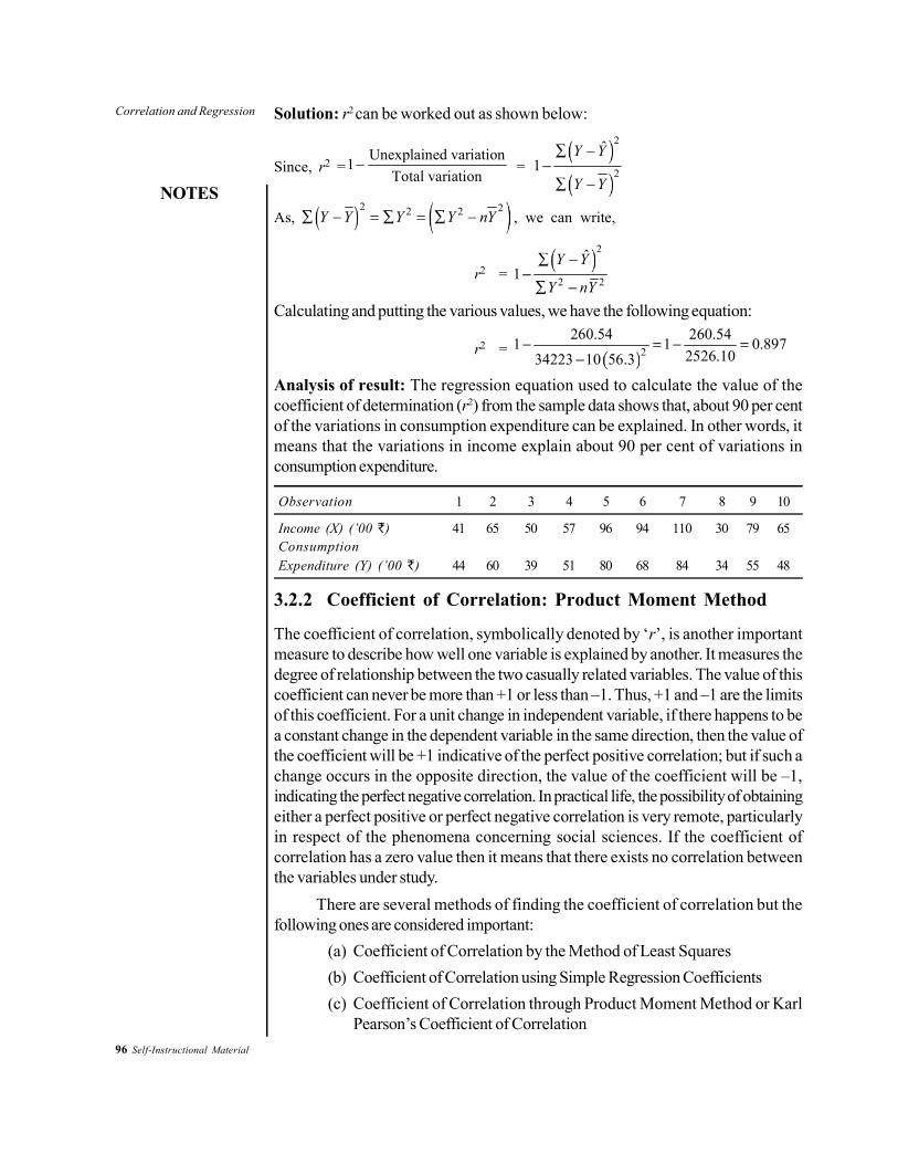
96 Self-Instructional Material
Correlation and Regression
NOTES
Solution: r2 can be worked out as shown below:
Since, r2 =Unexplained variation1
Total variation =
2
2
ˆ1
Y Y
Y Y
As,2 22 2Y Y Y Y nY , we can write,
r2 =
2
2 2
ˆ1
Y Y
Y nYCalculating and putting the various values, we have the following equation:
r2 = 2260.54 260.541 1 0.897
2526.1034223 10 56.3
Analysis of result: The regression equation used to calculate the value of thecoefficient of determination (r2) from the sample data shows that, about 90 per centof the variations in consumption expenditure can be explained. In other words, itmeans that the variations in income explain about 90 per cent of variations inconsumption expenditure.
Observation 1 2 3 4 5 6 7 8 9 10
Income (X) (’00 `) 41 65 50 57 96 94 110 30 79 65ConsumptionExpenditure (Y) (’00 `) 44 60 39 51 80 68 84 34 55 48
3.2.2 Coefficient of Correlation: Product Moment Method
The coefficient of correlation, symbolically denoted by ‘r’, is another importantmeasure to describe how well one variable is explained by another. It measures thedegree of relationship between the two casually related variables. The value of thiscoefficient can never be more than +1 or less than –1. Thus, +1 and –1 are the limitsof this coefficient. For a unit change in independent variable, if there happens to bea constant change in the dependent variable in the same direction, then the value ofthe coefficient will be +1 indicative of the perfect positive correlation; but if such achange occurs in the opposite direction, the value of the coefficient will be –1,indicating the perfect negative correlation. In practical life, the possibility of obtainingeither a perfect positive or perfect negative correlation is very remote, particularlyin respect of the phenomena concerning social sciences. If the coefficient ofcorrelation has a zero value then it means that there exists no correlation betweenthe variables under study.
There are several methods of finding the coefficient of correlation but thefollowing ones are considered important:
(a) Coefficient of Correlation by the Method of Least Squares(b) Coefficient of Correlation using Simple Regression Coefficients(c) Coefficient of Correlation through Product Moment Method or Karl
Pearson’s Coefficient of Correlation

Correlation and Regression
NOTES
Self-Instructional Material 97
Whichever of these above mentioned three methods we adopt, we get the samevalue of r.
(a) Coefficient of Correlation by the Method of Least SquaresUnder this method, first of all, the estimating equation is obtained using least squaremethod of simple regression analysis. The equation is worked out as,
ˆiY a bX
Total variation2
Y Y
Unexplained variation2ˆY Y
Explained variation2
Y Y
Then, by applying the following formulae, we can find the value of the coefficient ofcorrelation:
r =2 Explained variation
Total variationr
=Unexplained variation1
Total variation
=
2
2
ˆ1
Y Y
Y Y
This clearly shows that the coefficient of correlation happens to be the squarerootof the coefficient of determination.
Short-cut formula for finding the value of ‘r’ by the method of least squarescan be repeated and readily written as follows:
r =2
2 2a Y b XY nY
Y nYWhere, a = Y-intercept
b = Slope of the estimating equationX = Values of the independent variableY = Values of dependent variableY_
= Mean of the observed values of Yn = Number of items in the sample
(i.e., pairs of observed data)
The plus (+) or the minus (–) sign of the coefficient of correlation worked out by themethod of least squares, is related to the sign of ‘b’ in the estimating equation viz.,ˆ .iY a bX If ‘b’ has a minus sign, the sign of ‘r’ will also be minus but if ‘b’ has
a plus sign, then the sign of ‘r’ will also be plus. The value of ‘r’ indicates the degreealong with the direction of the relationship between the two variables X and Y.

98 Self-Instructional Material
Correlation and Regression
NOTES
(b) Coefficient of Correlation using Simple Regression CoefficientsUnder this method, the estimating equation of Y and the estimating equation of X isworked out using the method of least squares. From these estimating equations wefind the regression coefficient of X on Y, i.e., the slope of the estimating equation of
X (symbolically written as bXY) and this happens to be equal to X
Y
r and similarly,,
we find the regression coefficient of Y on X, i.e., the slope of the estimating equation
of Y (symbolically written as bYX) and this happens to be equal to Y
X
r σσ
. For finding
‘r’, the square root of the product of these two regression coefficients are workedout as stated below:1
r = .XY YXb b
= .X Y
Y Xr r
= 2r = r
As stated earlier, the sign of ‘r’ will depend upon the sign of the regressioncoefficients. If they have minus sign, then ‘r’ will take minus sign but the sign of ‘r’will be plus if regression coefficients have plus sign.
(c) Karl Pearson’s Coefficient or Product Moment MethodKarl Pearson’s method is the most widely used method of measuring the relationshipbetween two variables. This coefficient is based on the following assumptions:
(i) There is a linear relationship between the two variables which means thatstraight line would be obtained if the observed data are plotted on a graph.
(ii) The two variables are casually related which means that one of the variablesis independent and the other one is dependent.
(iii) A large number of independent causes are operating in both the variables soas to produce a normal distribution.
According to Karl Pearson, ‘r’ can be worked out as under:
r =X Y
XYnσ σ∑
Where, X = (X – X_
)Y = (Y – Y
_)
σX = Standard deviation of
X series and is equal to 2X
nσY = Standard deviation of
Y series and is equal to 2Y
n∑
n = Number of pairs of X and Y observed.

Correlation and Regression
NOTES
Self-Instructional Material 99
A short-cut formula, known as the Product Moment Formula, can be derived fromthe above stated formula as under:
r = X Y
XYnσ σ∑
= 2 2
XY
X Yn n
∑
∑ ∑⋅
n =2 2
XY
X Y
∑
∑ ∑
The above formulae are based on obtaining true means (viz. and X Y ) first andthen doing all other calculations. This happens to be a tedious task, particularly if thetrue means are in fractions. To avoid difficult calculations, we make use of theassumed means in taking out deviations and doing the related calculations. In such asituation, we can use the following formula for finding the value of ‘r’:2
(i) In case of ungrouped data:
r =2 22 2
.
.
dX dY dX dYn n n
dX dX dY dYn n n n
∑ ∑ ∑ − ⋅
∑ ∑ ∑ ∑ − −⋅
=2 2
2 2
. dX dYdX dYn
dX dYdX dY
n n
Where, ∑dX = ∑(X – XA) XA = Assumed average of X
∑dY = ∑(Y – YA) YA = Assumed average of Y
∑dX2 = ∑(X – XA)2
∑dY2 = ∑(Y – YA)2
∑dX . dY = ∑(X – XA) (Y – YA)
n = Number of pairs of observations of X and Y(ii) In case of grouped data:
r =2 22 2
. .fdX dY fdX fdYn n n
fdX fdX fdY fdYn n n n
∑ ∑ ∑ −
∑ ∑ ∑ ∑ − −

100 Self-Instructional Material
Correlation and Regression
NOTES
or r =2 2
2 2
.. fdX fdYfdX dYn
fdX fdYfdX fdYn n
∑ ∑ ∑ −
∑ ∑ ∑ − ∑ −
Where, ∑fdX.dY =0∑f (X – XA) (Y – YA)
∑fdX = ∑f (X – XA)
∑fdY = ∑f (Y – YA)
∑fdY2 = ∑f (Y – YA)2
∑fdX2 = ∑f (X – XA)2
n = Number of pairs of observations of X and Y.
3.2.3 Probable Error (P.E.) of the Coefficient of Correlation
Probable Error (P.E.) of r is very useful in interpreting the value of r and is workedout as under for Karl Pearson’s coefficient of correlation:
21P.E. 0.6745 rn
−=
If r is less than its P.E., it is not at all significant. If r is more than P.E., there iscorrelation. If r is more than 6 times its P.E. and greater than ± 0.5, then it isconsidered significant.Example 3.2:From the following data, calculate ‘r’ between X and Y applying the following threemethods:
(a) The method of least squares.(b) The method based on regression coefficients.(c) The product moment method of Karl Pearson.
Verify the obtained result of any one method with that of another.
X 1 2 3 4 5 6 7 8 9
Y 9 8 10 12 11 13 14 16 15
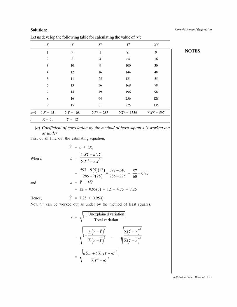
Correlation and Regression
NOTES
Self-Instructional Material 101
Solution:Let us develop the following table for calculating the value of ‘r’:
X Y X2 Y2 XY
1 9 1 81 9
2 8 4 64 16
3 10 9 100 30
4 12 16 144 48
5 11 25 121 55
6 13 36 169 78
7 14 49 196 98
8 16 64 256 128
9 15 81 225 135
n=9 ∑X = 45 ∑Y = 108 ∑X2 = 285 ∑Y2 = 1356 ∑XY = 597
∴ X_
= 5; Y_
= 12
(a) Coefficient of correlation by the method of least squares is worked outas under:
First of all find out the estimating equation,
Y = a + bXi
Where, b = 22
XY nX Y
X nX
=597 9 5 12 597 540
285 9 25 285 225 = 57 0.9560
=
and a = Y_
– bX_
= 12 – 0.95(5) = 12 – 4.75 = 7.25
Hence, Y = 7.25 + 0.95Xi
Now ‘r’ can be worked out as under by the method of least squares,
r =Unexplained variation1
Total variation−
=
2
2
ˆ1
Y Y
Y Y=
2
2
Y Y
Y Y
=2
22
a Y b XY nY
Y nY

102 Self-Instructional Material
Correlation and Regression
NOTES
This is as per short-cut formula,
r =( ) ( ) ( )
( )
2
2
7.25 108 0.95 597 9 12
1356 9 12
+ −
−
=783 567.15 1296
1356 1296
=54.15
60 = 0.9025 = 0.95
(b) Coefficient of correlation by the method based on regression coefficientsis worked out as under:
Regression coefficients of Y on X,
i.e., bYX = 22
XY nX Y
X nX
=597 9 5 12 597 540 57
285 225 60285 9 5Regression coefficient of X on Y,
i.e., bXY = 22
XY nX Y
Y nY
= 2597 9 5 12 597 540 57
1356 1296 601356 9 12Hence, r = .YX XYb b
=57 57 57 0.9560 60 60
× = =
(c) Coefficient of correlation by the product moment method of Karl Pearsonis worked out as under:
r =2 22 2
XY nX Y
X nX Y nY
=2 2
597 9 5 12
285 9 5 1356 9 12
=597 540 57
285 225 1356 1296 60 60=
57 0.9560
=
Hence, we get the value of r = 0.95. We get the same value applying the other twomethods also. Therefore, whichever method we apply, the results will be the same.

Correlation and Regression
NOTES
Self-Instructional Material 103
3.2.4 Some Other Measures
Two other measures are often talked about along with the coefficients ofdeterminations and that of correlation. These are as follows:
(a) Coefficient of Nondetermination: Instead of using coefficient ofdetermination, sometimes coefficient of nondetermination is used. Coefficientof non-determination (denoted by k2) is the ratio of unexplained variation tototal variation in the Y variable related to the X variable. Algebrically, we canwrite it as follows:
k2 =Unexplained variation
Total variation =
2
2
ˆY Y
Y Y
Concerning the data of Example 3.1 of this unit, coefficient of nondetermination willbe calculated as follows:
2 260.54 0.1032526.10
k
The value of k2 shows that about 10 per cent of the variation in consumption
expenditure remains unexplained by the regression equation we had worked out,viz., Y 14.000 + 0.616Xi. In simple terms, this means that variable other than X isresponsible for 10 per cent of the variations in the dependent variable Y in the givencase.Coefficient of nondetermination can as well be worked out as under:
k2 = 1 – r2
Accordingly, for Example 3.1, it will be equal to 1–0.897 = 0.103Note: Always remember that r2 + k2 = 1.
(b) Coefficient of Alienation: Based on k2, we can work out one more measurenamely the Coefficient of alienation, symbolically written as ‘k’. Thus,
Coefficient of alienation, i.e., ‘k’ = 2k
Unlike r + k2 = 1, the sum of ‘r’ and ‘k’ will not be equal to 1 unless one of the twocoefficients is 1 and in this case the remaining coefficients must be zero. In all othercases, ‘r’ + ‘k’ > 1. Coefficient of alienation is not a popular measure from practicalpoint of view and is used very rarely.
Spearman’s Rank CorrelationIf observations on two variables are given in the form of ranks and not as numericalvalues, it is possible to compute what is known as rank correlation between the twoseries.
The rank correlation, written as ρ, is a descriptive index of agreement betweenranks over individuals. It is the same as the ordinary coefficient of correlation computedon ranks, but its formula is simpler.
2
2
61
( 1)iD
n n

104 Self-Instructional Material
Correlation and Regression
NOTES
Here, n is the number of observations and Di, the positive difference between ranksassociated with the individuals i.
Like r, the rank correlation lies between –1 and +1.Example 3.3: The ranks given by two judges to 10 individuals are as follows:
Rank given byIndividual Judge I Judge II D D2
x y = x – y
1 1 7 6 362 2 5 3 93 7 8 1 14 9 10 1 15 8 9 1 16 6 4 2 47 4 1 3 98 3 6 3 99 10 3 7 4910 5 2 3 9
ΣD2 = 128
Solution: The rank correlation is given by,2
3 3
6 6 1281 1 1 0.776 0.22410 10
Dn n
The value of ρ = 0.224 shows that the agreement between the judges is not high.
Example 3.4: Consider Example 3.3 and compute r and compare.Solution: The simple coefficient of correlation r for the previous data is calculatedas follows:
x y x2 y2 xy
1 7 1 49 72 5 4 25 107 8 49 64 569 10 81 100 908 9 64 81 726 4 36 16 244 1 16 1 43 6 9 36 18
10 3 100 9 305 2 25 4 10
Σx = 55 Σy = 55 Σx2 = 385 Σy2 = 385 Σxy = 321
r =
55 55321 1010 10
2 255 55385 10 385 1010 10
= 18.5
82.5 82.5× =
18.582.5 = 0.224

Correlation and Regression
NOTES
Self-Instructional Material 105
This shows that the Spearman ρ for any two sets of ranks is the same as thePearson r for the set of ranks. But it is much easier to compute ρ.
Often, the ranks are not given. Instead, the numerical values of observationsare given. In such a case, we must attach the ranks to these values to calculate ρ.Example 3.5: On the basis of given table define correlation and calculate rank.
Marks in Marks in Rank in Rank inMaths Stats. Maths Stats. D D2
45 60 4 2 2 447 61 3 1 2 460 58 1 3 2 438 48 5 4 1 150 46 2 5 3 9
ΣD2 = 222
3
6 6 221 1 0.1125 5
Dn n
Solution: This shows a negative, though small, correlation between the ranks.If two or more observations have the same value, their ranks are equal and
obtained by calculating the means of the various ranks.If in this data, marks in maths are 45 for each of the first two students, the
rank of each would be 3 42+ = 3.5. Similarly, if the marks of each of the last two
students in statistics are 48, their ranks would be 4 52+ = 4.5
The problem takes the following shape:
R a n kMarks in Marks in x y D D2
Maths Stats
45 60 3.5 2 1.5 2.2545 61 3.5 1 2.5 6.2560 58 1 3 2 4.0038 48 5 4.5 0.5 0.2550 48 2 4.5 2.5 6.25
ΣD2 = 19
2
3
6 6 191 1 0.05120
Dn n
An elaborate formula which can be used in case of equal ranks is:
2 33
6 11
12D m m
n n .
Here, 3112
m mΣ( − ) is to be added to ΣD2 for each group of equal ranks, m being
the number of equal ranks each time.

106 Self-Instructional Material
Correlation and Regression
NOTES
For the given data, we have:(a) For series x, the number of equal ranks m = 2.(b) For series y, also, m = 2; so that,
ρ =3 3
3
6 1 11 21 (2 2) (2 2)12 125 5
=6 6 61 21
120 12 12
=6 221120×
− = –0.1
Example 3.6: Show by means of diagrams various cases of scatter expressingcorrelation between x, y.Solution:(a) Y
XO Negative slopeInverse linear relationship
High scatter low, negativer
(b) Y
XO Positive slopeDirect linear relationship
High scatter low, positiver
(c) Y
XO Slope = 0= 0r
(d) Y
XO No relationship – ~ 0r
(e) Y
XO Inversecurvilinear relationship
(f) Y
XO Directcurvilinear relationship

Correlation and Regression
NOTES
Self-Instructional Material 107
(g) Y
XO Perfect relationshipBut, = 0 because of non-linear relation
r
Correlation analysis helps us in determining the degree to which two or morevariables are related to each other.
When there are only two variables, we can determine the degree to whichone variable is linearly related to the other. Regression analysis helps in determiningthe pattern of relationship between one or more independent variables and a dependentvariable. This is done by an equation estimated with the help of data.
CHECK YOUR PROGRESS
1. What is Karl Pearson’s Method of Coefficient?2. Define Coefficient of Nondetermination.
3.3 MULTIPLE REGRESSION
The term ‘regression’ was first used in 1877 by Sir Francis Galton who made astudy that showed that the height of children born to tall parents will tend to moveback or ‘regress’ towards the mean height of the population. He designated theword regression as the name of the process of predicting one variable from theanother variable. He coined the term multiple regression to describe the process bywhich several variables are used to predict another. Thus, when there is a well-established relationship between variables, it is possible to make use of this relationshipin making estimates and to forecast the value of one variable (the unknown or thedependent variable) on the basis of the other variable/s (the known or the independentvariable/s). A banker, for example, could predict deposits on the basis of per capitaincome in the trading area of the bank. A marketing manager may plan his advertisingexpenditures on the basis of the expected effect on total sales revenue of a changein the level of advertising expenditure. Similarly, a hospital superintendent couldproject his need for beds on the basis of total population. Such predictions may bemade by using regression analysis. An investigator may employ regression analysisto test his theory having the cause and effect relationship. All this explains thatregression analysis is an extremely useful tool specially in problems of business andindustry involving predictions.
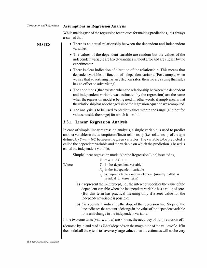
108 Self-Instructional Material
Correlation and Regression
NOTES
Assumptions in Regression AnalysisWhile making use of the regression techniques for making predictions, it is alwaysassumed that:
• There is an actual relationship between the dependent and independentvariables.
• The values of the dependent variable are random but the values of theindependent variable are fixed quantities without error and are chosen by theexperimentor.
• There is clear indication of direction of the relationship. This means thatdependent variable is a function of independent variable. (For example, whenwe say that advertising has an effect on sales, then we are saying that saleshas an effect on advertising).
• The conditions (that existed when the relationship between the dependentand independent variable was estimated by the regression) are the samewhen the regression model is being used. In other words, it simply means thatthe relationship has not changed since the regression equation was computed.
• The analysis is to be used to predict values within the range (and not forvalues outside the range) for which it is valid.
3.3.1 Linear Regression Analysis
In case of simple linear regression analysis, a single variable is used to predictanother variable on the assumption of linear relationship (i.e., relationship of the typedefined by Y = a + bX) between the given variables. The variable to be predicted iscalled the dependent variable and the variable on which the prediction is based iscalled the independent variable.
Simple linear regression model3 (or the Regression Line) is stated as,Yi = a + bXi + ei
Where, Yi is the dependent variableXi is the independent variableei is unpredictable random element (usually called as
residual or error term)
(a) a represent the Y-intercept, i.e., the intercept specifies the value of thedependent variable when the independent variable has a value of zero.(But this term has practical meaning only if a zero value for theindependent variable is possible).
(b) b is a constant, indicating the slope of the regression line. Slope of theline indicates the amount of change in the value of the dependent variablefor a unit change in the independent variable.
If the two constants (viz., a and b) are known, the accuracy of our prediction of Y(denoted by Y and read as Y--hat) depends on the magnitude of the values of ei. If inthe model, all the ei tend to have very large values then the estimates will not be very

Correlation and Regression
NOTES
Self-Instructional Material 109
good but if these values are relatively small, then the predicted values ( Y ) will tendto be close to the true values (Yi).Estimating the intercept and slope of the regression model (or estimating theregression equation)
The two constants or the parameters viz., ‘a’ and ‘b’ in the regression model for theentire population or universe are generally unknown and as such are estimated fromsample information. The following are the two methods used for estimation:
(a) Scatter diagram method(b) Least squares method
1. Scatter Diagram MethodThis method makes use of the Scatter diagram also known as Dot diagram. Scatterdiagram4 is a diagram representing two series with the known variable, i.e.,independent variable plotted on the X-axis and the variable to be estimated, i.e.,dependent variable to be plotted on the Y-axis on a graph paper (see Figure 3.2) toget the following information:
Income Consumption ExpenditureX Y
(Hundreds of Rupees) (Hundreds of Rupees)
41 4465 6050 3957 5196 8094 68
110 8430 3479 5565 48
The scatter diagram by itself is not sufficient for predicting values of thedependent variable. Some formal expression of the relationship between the twovariables is necessary for predictive purposes. For the purpose, one may simplytake a ruler and draw a straight line through the points in the scatter diagram and thisway can determine the intercept and the slope of the said line and then the line can
be defined as ˆiY a bX= + , with the help of which we can predict Y for a given value
of X. But there are shortcomings in this approach. For example, if five differentpersons draw such a straight line in the same scatter diagram, it is possible that theremay be five different estimates of a and b, specially when the dots are more dispersedin the diagram. Hence, the estimates cannot be worked out only through this approach.A more systematic and statistical method is required to estimate the constants of thepredictive equation. The least squares method is used to draw the best fit line.

110 Self-Instructional Material
Correlation and Regression
NOTES
0 20 40 60 80 100 120
120
100
80
60
40
20
x-axis
y-axis
Con
sum
ptio
n Ex
pend
iture
(00
Rs)
’
Fig. 3.2 Scatter Diagram
2. Least Square MethodLeast square method of fitting a line (the line of best fit or the regression line)through the scatter diagram is a method which minimizes the sum of the squaredvertical deviations from the fitted line. In other words, the line to be fitted will passthrough the points of the scatter diagram in such a way that the sum of the squaresof the vertical deviations of these points from the line will be a minimum.
The meaning of the least squares criterion can be easily understood throughreference to Figure 3.3, where the earlier figure in scatter diagram has beenreproduced along with a line which represents the least squares line fit to the data.
Fig. 3.3 Scatter Diagram, Regression Line and Short Vertical Lines Representing ‘e’
In Figure 3.3, the vertical deviations of the individual points from the line areshown as the short vertical lines joining the points to the least squares line. Thesedeviations will be denoted by the symbol ‘e’. The value of ‘e’ varies from one pointto another. In some cases it is positive, while in others it is negative. If the line drawnhappens to be least squares line, then the values of ie∑ is the least possible. It is so,because of this feature the method is known as Least Squares Method.

Correlation and Regression
NOTES
Self-Instructional Material 111
Why we insist on minimizing the sum of squared deviations is a question thatneeds explanation. If we denote the deviations from the actual value Y to the
estimated value Y as ˆ( – )Y Y or ei, it is logical that we want the 1
ˆ( – ) or ,n
ii
Y Y e=
Σ ∑ to
be as small as possible. However, mere examining 1
ˆ( – ) or ,n
ii
Y Y e=
Σ ∑ is inappropriate,
since any ei can be positive or negative. Large positive values and large negativevalues could cancel one another. But large values of ei regardless of their sign,
indicate a poor prediction. Even if we ignore the signs while working out 1
| |n
ii
e ,
the difficulties may continue. Hence, the standard procedure is to eliminate theeffect of signs by squaring each observation. Squaring each term accomplishestwo purposes viz., (i) it magnifies (or penalizes) the larger errors, and (ii) itcancels the effect of the positive and negative values (since a negative errorwhen squared becomes positive). The choice of minimizing the squared sum oferrors rather than the sum of the absolute values implies that there are manysmall errors rather than a few large errors. Hence, in obtaining the regressionline, we follow the approach that the sum of the squared deviations be minimumand on this basis work out the values of its constants viz., ‘a’ and ‘b’ also knownas the intercept and the slope of the line. This is done with the help of thefollowing two normal equations:5
ΣY = na + bΣXΣXY = aΣX + bΣX2
In the above two equations, ‘a’ and ‘b’ are unknowns and all other valuesviz., ∑X, ∑Y, ∑X2, ∑XY, are the sum of the products and cross products to becalculated from the sample data, and ‘n’ means the number of observations in thesample.
The following examples explain the Least squares method.
Example 3.7: Fit a regression line ˆiY a bX= + by the method of least squares to
the given sample information.Observations 1 2 3 4 5 6 7 8 9 10
Income (X) (’00 `) 41 65 50 57 96 94 110 30 79 65
ConsumptionExpenditure (Y) (’00 `) 44 60 39 51 80 68 84 34 55 48
Solution: We are to fit a regression line ˆiY a bX= + to the given data by the method
of Least squares. Accordingly, we work out the ‘a’ and ‘b’ values with the help ofthe normal equations as stated above and also for the purpose, work out ∑X, ∑Y,∑XY, ∑X2 values from the given sample information table on Summations forRegression Equation.

112 Self-Instructional Material
Correlation and Regression
NOTES
Summations for Regression Equation
Observations Income Consumption XY X2 Y2
X ExpenditureY
(’00 `) (’00 `)
1 41 44 1804 1681 19362 65 60 3900 4225 36003 50 39 1950 2500 15214 57 51 2907 3249 26015 96 80 7680 9216 64006 94 68 6392 8836 46247 110 84 9240 12100 70568 30 34 1020 900 11569 79 55 4345 6241 302510 65 48 3120 4225 2304
n = 10 ∑X = 687 ∑Y =563 ∑XY = 42358 ∑X2= 53173 ∑Y2 = 34223
Putting the values in the required normal equations we have,563 = 10a + 687b
42358 = 687a + 53173b
Solving these two equations for a and b we obtain,a = 14.000 and b = 0.616
Hence, the equation for the required regression line is,Y = a + bXi
or, Y = 14.000 + 0.616Xi
This equation is known as the regression equation of Y on X from which Y valuescan be estimated for given values of X variable.6
3.3.2 Checking the Accuracy of Equation: Regression Line inPrediction
After finding the regression line as stated above, one can check its accuracy also.The method to be used for the purpose follows from the mathematical property of aline fitted by the method of least squares viz., the individual positive and negativeerrors must sum to zero. In other words, using the estimating equation, one must findout whether the term ˆY Y is zero and if this is so, then one can reasonably besure that he has not committed any mistake in determining the estimating equation.
The problem of predictionWhen we talk about prediction or estimation, we usually imply that if the relationshipYi = a + bXi + ei exists, then the regression equation, ˆ
iY a bX provides a base formaking estimates of the value for Y which will be associated with particular valuesof X. In Example 3.7, we worked out the regression equation for the income andconsumption data as,
Y = 14.000 + 0.616Xi
On the basis of this equation we can make a point estimate of Y for any given valueof X. Suppose we wish to estimate the consumption expenditure of individuals with

Correlation and Regression
NOTES
Self-Instructional Material 113
income of 10,000. We substitute X = 100 for the same in our equation and get anestimate of consumption expenditure as follows:
ˆ 14.000 0.616 100 75.60Y
Thus, the regression relationship indicates that individuals with 10,000 of incomemay be expected to spend approximately 7,560 on consumption. But this is only anexpected or an estimated value and it is possible that actual consumption expenditureof same individual with that income may deviate from this amount and if so, then ourestimate will be an error, the likelihood of which will be high if the estimate is appliedto any one individual. The interval estimate method is considered better and itstates an interval in which the expected consumption expenditure may fall. Rememberthat the wider the interval, the greater the level of confidence we can have, but thewidth of the interval (or what is technically known as the precision of the estimate)is associated with a specified level of confidence and is dependent on the variability(consumption expenditure in our case) found in the sample. This variability is measuredby the standard deviation of the error term, ‘e’, and is popularly known as thestandard error of the estimate.
3.3.3 Standard Error of the Estimate
Standard error of estimate is a measure developed by the statisticians for measuringthe reliability of the estimating equation. Like the standard deviation, the StandardError (S.E.) of Y measures the variability or scatter of the observed values of Yaround the regression line. Standard Error of Estimate (S.E. of Y ) is worked out asunder:
S.E. of 2 2ˆ( )ˆ (or )
2 2eY Y e
Y Sn n
where, S.E. of Y (or Se) = Standard error of the estimate
Y = Observed value of Y
Y = Estimated value of Y
e = The error term = (Y– Y )
n = Number of observations in the sample
Note: In the above formula, n – 2 is used instead of n because of the fact that two degrees offreedom are lost in basing the estimate on the variability of the sample observations aboutthe line with two constants viz., ‘a’ and ‘b’ whose position is determined by those samesample observations.
The square of the Se, also known as the variance of the error term, is the basic measure ofreliability. The larger the variance, the more significant are the magnitudes of the e’s and theless reliable is the regression analysis in predicting the data.
Interpreting the standard error of estimate and finding the confidencelimits for the estimate in large and small samples
The larger the S.E. of estimate (SEe), the greater happens to be the dispersion,or scattering, of given observations around the regression line. But if the S.E. of

114 Self-Instructional Material
Correlation and Regression
NOTES
estimate happens to be zero then the estimating equation is a ‘perfect’ estimator(i.e., cent per cent correct estimator) of the dependent variable.In case of large samples, i.e., where n > 30 in a sample, it is assumed that theobserved points are normally distributed around the regression line and we mayfind,
68 per cent of all points within ˆ 1Y SEe limits
95.5 per cent of all points within ˆ 2Y SEe limits
99.7 per cent of all points within ˆ 3Y SEe limitsThis can be stated as,
(a) The observed values of Y are normally distributed around each estimatedvalue of Y and;
(b) The variance of the distributions around each possible value of Y is thesame.
In case of small samples, i.e., where n ≤ 30 in a sample the ‘t’ distribution isused for finding the two limits more appropriately.This is done as follows:
Upper limit = Y + ‘t’ (SEe)
Lower limit = Y – ‘t’ (SEe)
Where, Y = The estimated value of Y for a given value of X.SEe = The standard error of estimate.
‘t’ = Table value of ‘t’ for given degrees of freedom for aspecified confidence level.
Some other details concerning simple regressionSometimes the estimating equation of Y also known as the Regression equationof Y on X, is written as follows:
Y Y = Yi
Xr X X
or, Y = Yi
Xr X X Y
Where, r = Coefficient of simple correlation between X and YσY = Standard deviation of YσX = Standard deviation of XX_
= Mean of XY_
= Mean of Y
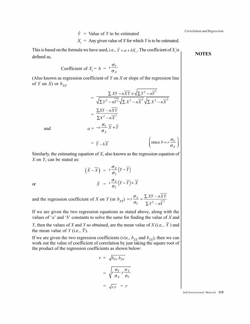
Correlation and Regression
NOTES
Self-Instructional Material 115
Y = Value of Y to be estimatedXi = Any given value of X for which Y is to be estimated.
This is based on the formula we have used, i.e., ˆiY a bX . The coefficient of Xi is
defined as,
Coefficient of Xi = b = Y
Xr
(Also known as regression coefficient of Y on X or slope of the regression lineof Y on X) or bYX.
= 22
2 22 2 2 2
XY nXY Y nY
Y nY X nX X nX
= 22
XY nX Y
X nX
and a = Y
Xr X Y
= Y bX since Y
Xb r
Similarly, the estimating equation of X, also known as the regression equation ofX on Y, can be stated as:
X X = X
Yr Y Y
or X = X
Yr Y Y X
and the regression coefficient of X on Y (or bXY) 22X
Y
XY nX YrY nY
If we are given the two regression equations as stated above, along with thevalues of ‘a’ and ‘b’ constants to solve the same for finding the value of X andY, then the values of X and Y so obtained, are the mean value of X (i.e., X ) andthe mean value of Y (i.e., Y
_).
If we are given the two regression coefficients (viz., bXY and bYX), then we canwork out the value of coefficient of correlation by just taking the square root ofthe product of the regression coefficients as shown below:
r = .YX XYb b
= .Y X
X Yr r
= .r r = r

116 Self-Instructional Material
Correlation and Regression
NOTES
The (±) sign of r will be determined on the basis of the sign of the regressioncoefficients given. If regression coefficients have minus sign then r will be takenwith minus (–) sign and if regression coefficients have plus sign then r will betaken with plus (+) sign. (Remember that both regression coefficients willnecessarily have the same sign whether it is minus or plus for their sign isgoverned by the sign of coefficient of correlation.)Example 3.8: Given is the following information:
X YMean 39.5 47.5Standard Deviation 10.8 17.8
Simple correlation coefficient between X and Y is = + 0.42Find the estimating equation of Y and X.Solution:Estimating equation of Y can be worked out as,
Y Y = ( )Yi
Xr X Xσ
σ−
or Y = ( )Yi
Xr X X Yσ
σ− +
= ( )17.80.42 39.5 47.510.8 iX − +
= 0.69 27.25 47.5iX
= 0.69Xi + 20.25Similarly, the estimating equation of X can be worked out as under:
X X = ( )Xi
Yr Y Yσ
σ−
or X = ( )Xi
Yr Y Y Xσ
σ− +
or = ( )10.80.42 47.5 39.517.8 iY − +
= 0.26Yi – 12.35 + 39.5= 0.26Yi + 27.15
Example 3.9: Given is the following data:Variance of X = 9Regression equations:
4X – 5Y + 33 = 020X – 9Y – 107 = 0
Find: (a) Mean values of X and Y.(b) Coefficient of Correlation between X and Y.(c) Standard deviation of Y.

Correlation and Regression
NOTES
Self-Instructional Material 117
Solution:(a) For finding the mean values of X and Y, we solve the two given regressionequations for the values of X and Y as follows:
4X – 5Y + 33 = 0 (1)20X – 9Y –107 = 0 (2)
If we multiply equation (1) by 5, we have the following equations:20X – 25Y = –165 (3)20X – 9Y = 107 (2)– + –
– 16Y = –272Subtracting equation (2) from (3):or Y = 17Putting this value of Y in equation (1) we have,
4X = – 33 + 5(17)
or X =33 85 52 13
4 4
Hence, X_
= 13 and Y = 17(b) For finding the coefficient of correlation, first of all we presume one of thetwo given regression equations as the estimating equation of X. Let equation 4X –5Y + 33 = 0 be the estimating equation of X, then we have,
5 33ˆ4 4
iYX
and
From this we can write bXY 54
The other given equation is then taken as the estimating equation of Y and canbe written as,
20 107ˆ9 9
iXY
and from this we can write bYX 209
If the above equations are correct then r must be equal to,
r = 5 / 4 20 / 9 25 / 9 = 5/3 = 1.6which is an impossible equation, since r can in no case be greater than 1. Hence,we change our supposition about the estimating equations and by reversing it, were-write the estimating equations as under:
9 107ˆ20 20
iYX

118 Self-Instructional Material
Correlation and Regression
NOTES
and4 33ˆ
5 5iXY
Hence, r = 9 / 20 4 / 5
= 9 / 25
= 3/5= 0.6
Since, regression coefficients have plus signs, we take r = + 0.6(c) Standard deviation of Y can be calculated as follows:
Variance of X = 9∴ Standard deviation of X = 3
YYX
Xb r =
4 0.6 0.25 3
YY
Hence, σY = 4Alternatively, we can work it out as under:
XXY
Yb r =
9 1.80.620 3
Y
Y
σσ
= =
Hence, σY = 4.
3.3.4 Predicting an Estimate, and its Preciseness
Regression analysis helps predict the most likely value of the dependent variablecorresponding to a given, known, value of the independent variable. This is achievedthrough the predictive function of the regression equation. Substituting any knownX value in and solving it yields a Ye value, which serves as the most likely estimate ofY corresponding to that X value.
Accordingly, a Ye value so estimated may also be read as the expected valueof Y against a given value of X. For example, for a given value of X = 10, Ye = 2.823+ 0.252 (10) = 5.343 is the expected value based on the linear relationship.
Alternatively, the estimated or expected Ye value for a given value of X canalso be found by using either of the regression equations
or ,e
e
Y Y b X X
Y Y b X X (3.1)
The use of Eq. (3.1) do not require knowing the value of a. Instead, the value of band mean X and Y based on the available data suffice.

Correlation and Regression
NOTES
Self-Instructional Material 119
Equation 3.1 is obtained as under:SinceYe = a + bX,
substituting ( )Y Y bX bX= − + for a gives
( )eY Y bX bX= − +
or
( )eY Y b X X= + −
or
( ).eY Y b X X− = −
Given the estimating characteristic of (Eq. 3.1) as used in the manner demonstratedabove, it is important to carefully note the following:
(a) An estimated Ye value against a given value of X obtained by using (Eq. 3.1)will be the best approximation as long as the basic conditions affecting therelationship between X and Y, do not change.
(b) An estimated Ye value may not be exactly the same as it is actually observed.The difference between an estimated Ye value and the corresponding observedY value will depend on the extent of scatter of various points around the lineof best fit.
(c) The closer the sample paired points (Y X) scattered around the line of best fit,the smaller the difference between the estimated Ye and observed Y values,and vice versa. On the whole, the lesser the scatter of the various pointsaround (and, consequently, the lesser the vertical distance by which thesedeviate from) the line of best fit, the more likely it is that an estimated Ye valueis close to the corresponding observed Y value.
(d) The estimated Ye values will be the same as the observed Y values only whenall the points on the scatter diagram form a straight line. If this were to be so,the rice yield based on the use of a given quantity of fertilizer could be estimatedwith 100 per cent accuracy. Since some of the points must lie above andsome below the straight line, perfect prediction is practically non-existent inthe case of most business and economic variables.It is evident that the estimated values of one variable based on the known
values of the other variable are bound to be different from those that are actuallyobserved. The former are thus always in error compared to the latter. The smallerthis error, the more precise and reliable the estimate, and vice versa. That is, thepreciseness of an estimate can be known by measuring the magnitude of the saiderrors. The magnitude of error in an estimate is thus called the error of estimate.

120 Self-Instructional Material
Correlation and Regression
NOTES
3.3.5 Multiple and Partial Correlation
This section describes the measure of simple linear correlation in the following ways:
a. In Terms of Coefficient of Multiple DeterminationJust as there was measure of simple linear correlation in the two-variable case, ameasure of linear multiple correlation (or just multiple correlation) in the three-variable case is defined in terms of the coefficient of multiple determination. Denotedas 2
1.23R , it uses 21.23S in its computation, the same way as R2 uses 2
Y XS in the two-variable case.
The coefficient of multiple determination 21.23R holds the same significance as
that of the coefficient of determination R2 (or 21.2R ) does in the two-variable case.
Here, the former represents the proportion of total variations in the dependent variableX1 which is explained by the variations in the two independent variables X2 and X3.
Thus, the coefficient of multiple correlation, denoted as r1.23, in the case ofthree variables is defined as
22 1.23
1.23 1.23 21
1 .S
r RS (3.2)
For the illustration under consideration,
21.23
1.23 21
0.325131 1 0.9260.2.2801
Sr
S
The subscripts used in the coefficient of determination 21.23R (or r1.23) are the
same as for S1.23. Use of 1 before the decimal point refers to the dependent variableX1 and that of 2 and 3 after the decimal point to the two independent variables X2
and X3. The subscripts used thus make it evident that 21.23R (or 2
1.23r ) is a measure ofthe proportion of total variations in the dependent variable X1 explained by thecombined influence of the variations in the two independent variables X2 and X3.
When either X2 or X3 is the dependent variable in place of X1, the remainingtwo being the independent variables, the corresponding multiple correlation coefficientsare
22 2.13
2.13 2.13 22
1 .S
r RS
and2
2 3.123.12 3.12 2
3
1 .S
r RS (3.3)
respectively.
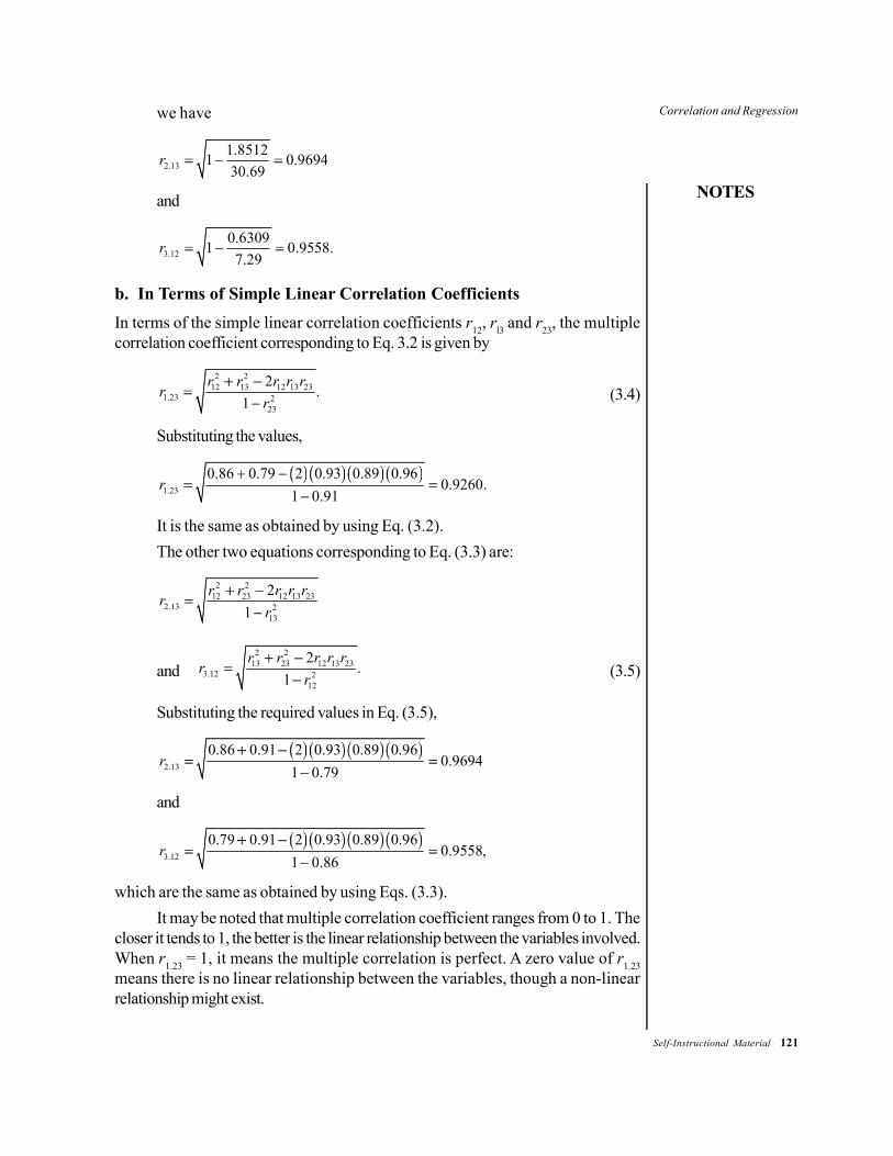
Correlation and Regression
NOTES
Self-Instructional Material 121
we have
2.131.85121 0.969430.69
r
and
3.120.63091 0.9558.7.29
r
b. In Terms of Simple Linear Correlation CoefficientsIn terms of the simple linear correlation coefficients r12, rl3 and r23, the multiplecorrelation coefficient corresponding to Eq. 3.2 is given by
2 212 13 12 13 23
1.23 223
2.
1r r r r r
rr (3.4)
Substituting the values,
1.23
0.86 0.79 2 0.93 0.89 0.960.9260.
1 0.91r
It is the same as obtained by using Eq. (3.2).The other two equations corresponding to Eq. (3.3) are:
2 212 23 12 13 23
2.13 213
21
r r r r rr
r
and2 2
13 23 12 13 233.12 2
12
2.
1r r r r r
rr (3.5)
Substituting the required values in Eq. (3.5),
2.13
0.86 0.91 2 0.93 0.89 0.960.9694
1 0.79r
and
3.12
0.79 0.91 2 0.93 0.89 0.960.9558,
1 0.86r
which are the same as obtained by using Eqs. (3.3).It may be noted that multiple correlation coefficient ranges from 0 to 1. The
closer it tends to 1, the better is the linear relationship between the variables involved.When r1.23 = 1, it means the multiple correlation is perfect. A zero value of r1.23means there is no linear relationship between the variables, though a non-linearrelationship might exist.

122 Self-Instructional Material
Correlation and Regression
NOTES
Partial CorrelationWe know that the two partial regression coefficients (b12.3 and b13.2) serve asmeasures of the net influence of the two independent variables X2 and X3 on thevalues of the dependent variable X1. In the same way, the partial correlationcoefficients, denoted as rl2.3 and r13.2, are measures of the net correlation betweenthe dependent variable and one of the two independent variables (holding the otherindependent variable constant, or ignoring its effect on the dependent one).
Thus, the subscript to the right of the decimal point indicates the variablewhich is held constant or whose relationship with the dependent variable has beenignored, while those to the left of the decimal point indicate the two variables betweenwhich net correlation is computed. Accordingly, r12.3 represents the partialcorrelation between X1 and X2, holding X3 constant. Likewise, r13.2 represents partialcorrelation between X1 and X3, holding X2 constant.
To obtain a measure of, say, r13.2 (or the coefficient of partial determination2
13.2R ), note the following:
(i) 21.23S represents the variance in X1 not explained by the two independent
variables X2 and X3. That is, it is a measure of variance in X1 thatremains unexplained even after adding the second independent variableX3.
(ii) 21.23S is similar to 2
1.2S for the two-variable case (X1 and X2, X1 beingdependent), where the latter represents the variance in X1 not explainedby the single independent variable X2.
(iii) The difference between 21.2S and 2
1.23S is the reduction in the unexplainedvariance in X1 obtained by adding the second independent variable X3 inthe estimating equation.
(iv) It is this reduction in unexplained variance which is used as a measureof net correlation between X1 and X3, when the influence of X2 both onX1 and X3 has been taken into account.
Thus, the coefficient of partial determination between X1 and X3 (eliminatingthe effect of X2) is computed as
22 1.2313.2 2
1.2
1 ,S
RS
so that the coefficient of partial correlation is
21.23
13.2 21.2
1 .S
rS (3.6)
It may be recalled that 21.2S is the square of standard error of estimate S1.2, as
against 21S , as the variance of X1.

Correlation and Regression
NOTES
Self-Instructional Material 123
Substituting the values,
13.20.325371 1 0.99593 0.0638.0.3267
r
Similarly,
22 1.23
12.3 21.3
1S
RS and
21.23
12.3 21.3
1 .S
rS (3.7)
It may be noted that r12.3 and r13 2 take the same signs as the correspondingpartial regression coefficients b12.3 and b13.2.
The results of Eqs. (3.6) and (3.7) can also be obtained in terms of the simplecorrelation coefficients as
13 12 2313.2 2 2
12 231 1
r r rr
r r
and 12 13 23
12.3 2 213 23
.1 1
r r rr
r r (3.8)
Similarly,23 12 23
23.1 2 212 131 1
r r rr
r r
Substituting the values of simple correlation coefficients in the first of the twoEqs. (3.8), we have
13.2
0.8911 0.9256 0.95540.068,
1 0.8568 1 0.9128r
which is approximately the same as obtained from Eq. (3.6).Likewise,
12.3
0.9256 0.8911 0.95540.5537.
1 0.7941 1 0.9128r
For the three-variable case, an interesting result connecting the multiple andpartial correlation coefficients lies in
2 2 21.23 12 13.21 1 1R r r
or
2 2 21.23 12 13.21 1 1 .R r r

124 Self-Instructional Material
Correlation and Regression
NOTES
CHECK YOUR PROGRESS
3. What is the least square method of fitting a line?4. What is standard error of estimate?
3.4 SUMMARY
• Correlation analysis looks at the indirect relationships and establishes thevariables which are most closely associated with a given data or mindset. It isthe process of finding how accurately the line fits using the observations.Correlation analysis can be referred to as the statistical tool used to describethe degree to which one variable is related to another. The relationship, if any,is usually assumed to be a linear one. In fact, the word correlation refers tothe relationship or the interdependence between two variables.
• The theory by means of which quantitative connections between two sets ofphenomena are determined is called the ‘Theory of Correlation’. On thebasis of the theory of correlation, you can study the comparative changesoccurring in two related phenomena and their cause-effect relation can alsobe examined. Thus, correlation is concerned with relationship between tworelated and quantifiable variables and can be positive or negative.
• On the basis of the theory of correlation, one can study the comparativechanges occurring in two related phenomena and their cause-effect relationcan be examined. It should, however, be borne in mind that relationship like‘black cat causes bad luck’, ‘filled up pitchers result in good fortune’ andsimilar other beliefs of the people cannot be explained by the theory ofcorrelation, since they are all imaginary and are incapable of being justifiedmathematically.
• Correlation can either be positive or it can be negative. Whether correlationis positive or negative would depend upon the direction in which the variablesare moving. If both variables are changing in the same direction, then correlationis said to be positive, but, when the variations in the two variables take placein opposite direction, the correlation is termed as negative.
• The coefficient of determination (symbolically indicated as r2, though somepeople would prefer to put it as R2) is a measure of the degree of linearassociation or correlation between two variables, say X and Y, one of whichhappens to be independent variable and the other being dependent variable.
• Coefficients of determination is that fraction of the total variation of Y whichis explained by the regression line. In other words, coefficient of determinationis the ratio of explained variation to total variation in the Y variable related tothe X variable.

Correlation and Regression
NOTES
Self-Instructional Material 125
• The coefficient of determination can have a value ranging from zero to one.The value of one can occur only if the unexplained variation is zero, whichsimply means that all the data points in the Scatter diagram fall exactly on theregression line.
• The coefficient of correlation, symbolically denoted by ‘r’, is another importantmeasure to describe how well one variable is explained by another. It measuresthe degree of relationship between the two casually related variables. Thevalue of this coefficient can never be more than +1 or less than –1. Thus, +1and –1 are the limits of this coefficient.
• There are several methods of finding the coefficient of correlation. Some ofthe important methods include: a) Coefficient of Correlation by the Methodof Least Squares b) Coefficient of Correlation using Simple RegressionCoefficients c) Coefficient of Correlation through Product Moment Methodor Karl Pearson’s Coefficient of Correlation
• Probable Error (P.E.) of r is very useful in interpreting the value of r and isworked out as under for Karl Pearson’s coefficient of correlation:
21P.E. 0.6745 rn
−=
• Two other measures are often talked about along with the coefficients ofdeterminations and that of correlation. These are as follows:(a) Coefficient of Non-determination (b) Coefficient of Alienation.
• If observations on two variables are given in the form of ranks and not asnumerical values, it is possible to compute what is known as rank correlationbetween the two series. The rank correlation, written as r, is a descriptiveindex of agreement between ranks over individuals. It is the same as theordinary coefficient of correlation computed on ranks, but its formula is simpler.
2
2
61
( 1)iD
n n• Sir Francis Galton coined the term multiple regression to describe the process
by which several variables are used to predict another. Thus, when there is awell-established relationship between variables, it is possible to make use ofthis relationship in making estimates and to forecast the value of one variable(the unknown or the dependent variable) on the basis of the other variable/s(the known or the independent variable/s).
• Scatter Diagram Method makes use of the Scatter diagram also known asDot diagram. Scatter diagram is a diagram representing two series with theknown variable, i.e., independent variable plotted on the X-axis and the variableto be estimated, i.e., dependent variable to be plotted on the Y-axis on a graphpaper.
• Least square method of fitting a line (the line of best fit or the regression line)through the scatter diagram is a method which minimizes the sum of the

126 Self-Instructional Material
Correlation and Regression
NOTES
squared vertical deviations from the fitted line. In other words, the line to befitted will pass through the points of the scatter diagram in such a way thatthe sum of the squares of the vertical deviations of these points from the linewill be a minimum.
3.5 KEY TERMS
• Correlation analysis: It is a statistical tool, used to describe the degree towhich one variable is related to another.
• Coefficient of determination: It is a measure of the degree of linearassociation or correlation between two variables, one of which must be anindependent variable and the other, a dependent variable.
• Coefficient of correlation: It measures the degree of relationship betweenthe two casually related variables.
• Regression analysis: It is a relationship used for making estimates andforecasts about the value of one variable (the unknown or the dependentvariable) on the basis of the other variable/s (the known or the independentvariable/s).
• Scatter diagram: It is a diagram used to represent two series with the knownvariables, i.e., independent variable plotted on the X-axis and the variable tobe estimated, i.e., dependent variable to be plotted on the Y-axis on a graphpaper for the given information.
• Standard error of the estimate: It is a measure developed by statisticiansfor measuring the reliability of the estimating equation.
3.6 ANSWERS TO ‘CHECK YOUR PROGRESS’
1. Karl Pearson’s method is the most widely used method of measuring therelationship between two variables. The coefficient is based on variousassumptions. There is a linear relationship between the two variables whichmeans that straight line would be obtained if the observed data are plotted ona graph.
2. Coefficient of non-determination (denoted by k2) is the ratio of unexplainedvariation to total variation in the Y variable related to the X variable.Algebraically, we can write it as follows:
k2 = Unexplained variation
Total variation =
2
2
ˆY Y
Y Y
3. Least square method of fitting a line (the line of best fit or the regression line)through the scatter diagram is a method which minimizes the sum of thesquared vertical deviations from the fitted line.

Correlation and Regression
NOTES
Self-Instructional Material 127
4. Standard error of estimate is a measure developed by the statisticians formeasuring the reliability of the estimating equation. Like the standard deviation,the Standard Error (S.E.) of measures the variability or scatter of the observedvalues of Y around the regression line.
3.7 QUESTIONS AND EXERCISES
Short-Answer Questions1. What is the importance of correlation analysis?2. How will you determine the coefficient of determination?3. What is the relationship between coefficient of nondetermination and
coefficient of alienation?4. List the basic precautions and limitations of regression and correlation analyses.5. What is Spearman’s rank correlation?6. Define regression analysis.7. How will you predict the value of dependent variable?8. Differentiate between scatter diagram and least square method.9. Can the accuracy of estimated equation be checked? Explain.
10. How is the standard error of estimate calculated?
Long-Answer Questions1. Explain the method to calculate the coefficient of correlation using simple
regression coefficient.2. Describe Karl Pearson’s method of measuring coefficient of correlation.3. Calculate correlation coefficient and the two regression lines for the following
information:Ages of Wives (in years)
10–20 20–30 30–40 40–50 Total
Ages of 10–20 20 26 — — 46Husbands 20–30 8 14 37 — 59(in 30–40 — 4 18 3 25years) 40–50 — — 4 6 10
Total 28 44 59 9 140
4. Two random variables have the regression with equations,3X + 2Y – 26 = 06X + Y – 31 = 0Find the mean value of X as well as of Y and the correlation coefficientbetween X and Y. If the variance of X is 25, find σY from the data givenabove.

128 Self-Instructional Material
Correlation and Regression
NOTES
5. (i) Give one example of a pair of variables which would have,(a) An increasing relationship(b) No relationship(c) A decreasing relationship
(ii) Suppose that the general relationship between height in inches (X) andweight in kg (Y) is Y’ = 10 + 2.2 (X). Consider that weights of persons ofa given height are normally distributed with a dispersion measurable byσe = 10 kg.
(a) What would be the expected weight for a person whose height is65 inches?
(b) If a person whose height is 65 inches should weigh 161 kg., whatvalue of e does this represent?
(c) What reasons might account for the value of e for the person incase (b)?
(d) What would be the probability that someone whose height is 70inches would weigh between 124 and 184 kg?
6. Calculate correlation coefficient from the following results:n = 10; ΣX = 140; ΣY = 150
Σ(X – 10)2 = 180; (Y – 15)2 = 215Σ(X – 10) (Y – 15)) = 60
7. Examine the following statements and state whether each one of thestatements is true or false, assigning reasons to your answer.
(a) If the value of the coefficient of correlation is 0.9 then this indicates that90 per cent of the variation in dependent variable has been explained byvariation in the independent variable.
(b) It would not be possible for a regression relationship to be significant ifthe value of r2 was less than 0.50.
(c) If there is found a high significant relationship between the two variablesX and Y, then this constitutes definite proof that there is a casual relationshipbetween these two variables.
(d) Negative value of the ‘b’ coefficient in a regression relationship indicatesa weaker relationship between the variables involved than would a positivevalue for the ‘b’ coefficient in a regression relationship.
(e) If the value for the ‘b’ coefficient in an estimating equation is less than0.5, then the relationship will not be a significant one.
(f) r2 + k2 is always equal to one. From this it can also be inferred that r+ k is equal to one
2
2
= coefficient of correlation; = coefficient of determination
= coefficient of alienation; = coefficient of non-determination
r r
k k

Correlation and Regression
NOTES
Self-Instructional Material 129
3.8 FURTHER READING
Chance, William A. 1969. Statistical Methods for Decision Making. Illinois: RichardD Irwin.
Chandan, J.S. 1998. Statistics for Business and Economics. New Delhi: VikasPublishing House.
Chandan, J.S., Jagjit Singh and K.K. Khanna. 1995. Business Statistics, SecondEdition. New Delhi: Vikas Publishing House.
Elhance, D.N. 2006. Fundamental of Statistics. Allahabad: Kitab Mahal.Freud, J.E., and F.J. William. 1997. Elementary Business Statistics – The Modern
Approach. Third Edition. New Jersey: Prentice-Hall International.Goon, A.M., M.K. Gupta, and B. Das Gupta. 1983. Fundamentals of Statistics.
Vols. I & II, Kolkata: The World Press Pvt. Ltd.
References1. Remember the short-cut formulae to workout bXY and bYX:
2 2XYXY nXY
bY nY
∑ −=
∑ −
and 2 2YXXY nXY
bn XX
∑ −=
∑ −
2. In case we take assumed mean to be zero for X variable as for Y variable then ourformula will be as under:
r = 2 22 2
XY X Yn n n
X X Y Yn n n n
∑ ∑ ∑ −
∑ ∑ ∑ ∑ − −
or r = 2 22 2
XY XYn
X YX Yn n
∑−
∑ ∑− −
r = 2 2 2 2
XY nXY
X nX Y nY
3. Usually the estimate of Y denoted by Y is written as,
ˆiY a bX
on the assumption that the random disturbance to the system averages out or hasan expected value of zero (i.e., e = 0) for any single observation. This regressionmodel is known as the Regression line of Y on X from which the value of Y can beestimated for the given value of X.

130 Self-Instructional Material
Correlation and Regression
NOTES
4.
(1)(2) (3) (4) (5)
Five possible forms which the Scatter diagram may assume has been depicted inthe above five diagrams. First diagram is indicative of perfect positive relationship,Second shows perfect negative relationship, Third shows no relationship, Fourthshows positive relationship and Fifth shows negative relationship between thetwo variables under consideration.
5. If we proceed centering each variable, i.e., setting its origin at its mean, then thetwo equations will be as under:
∑Y = na + b∑X
∑XY = a∑X + b∑X2
But since ∑Y and ∑X will be zero, the first equation and the first term of thesecond equation will disappear and we shall simply have the following equations:
∑XY = b∑X2
b = ∑XY/∑X2
The value of ‘a’ can then be worked out as:
a = Y_ – bX_
6. It should be pointed out that the equation used to estimate the Y variable valuesfrom values of X should not be used to estimate the values of X variable fromgiven values of Y variable. Another regression equation (known as the regressionequation of X on Y of the type X = a + bY) that reverses the two value should beused if it is desired to estimate X from value of Y.
Normal Distribution
NOTES
Self-Instructional Material 131
UNIT 4 NORMAL DISTRIBUTION
Structure4.0 Introduction4.1 Unit Objectives4.2 Meaning, Significance and Characteristics of Normal Curve
4.2.1 Normal Probability Curve and its Uses4.2.2 Uses of Normal Probability Curve: Computing Percentiles and Percentile
Ranks4.3 Need, Importance and Significance of the Difference between Means
and other Statistics4.3.1 Null Hypothesis4.3.2 Z-test4.3.3 t-Test4.3.4 Sampling Distribution of Means4.3.5 Confidence Intervals and Levels of Significance4.3.6 Two-Tailed and One-Tailed Tests of Significance
4.4 Summary4.5 Key Terms4.6 Answers to ‘Check Your Progress’4.7 Questions and Exercises4.8 Further Reading
4.0 INTRODUCTION
In this unit, you will learn about the significant characteristics and applications ofnormal distribution. Normal distribution is the most common type of distribution.Typically, a normal distribution is a very important statistical data distribution patternoccurring in many natural phenomena, such as height, blood pressure, lengths ofobjects produced by machines. Certain data, when graphed as a histogram (data onthe horizontal axis, amount of data on the vertical axis), creates a bell-shaped curveknown as a normal curve or normal distribution.
Thus, the normal distribution is a very important class of statistical distribution.All normal distributions are symmetric and have bell shaped density curves with asingle peak. Specifically, in any normal distribution, two quantities have to be specified,the mean m where the peak of the density occurs and the standard deviation s whichindicates the spread or girth of the bell curve.
You will also learn about Z-test and t-test for independent and dependentgroup in this unit. A Z-test is any statistical test for which the distribution of the teststate can be approximated by normal distribution under the null hypothesis. Typically,it is a statistical test used to determine whether two population means are differentwhen the variances are known and the sample size is large. Like normal distribution,t distribution is also symmetrical but happens to be flatter than normal distribution.The t-test can be used to compare a sample mean to an accepted value (of apopulation mean) or it can be used to compare the means of two sample sets. For

132 Self-Instructional Material
Normal Distribution
NOTES
applying t-test in the context of small samples, the t value is calculated first of all andthen the calculated value is compared with the table value of t at certain level ofsignificance for given degrees of freedom. The t-test is used when two conditionsare fulfilled, such as when the sample size is less than 30, i.e., when n ≤ 30 andwhen the population standard deviation (σp) must be unknown.
4.1 UNIT OBJECTIVES
After going through this unit, you will be able to:• Explain the significance and characteristics of normal distribution• Discuss how to measure the area under the normal curve• Assess the significance of Z-test• Explain the steps of Z-test for independent and dependent group• Discuss the importance of t-test• Discuss sampling distribution of means• Explain the two-tailed and one-tailed tests of significance
4.2 MEANING, SIGNIFICANCE ANDCHARACTERISTICS OF NORMAL CURVE
Among all the probability distributions, the normal probability distribution is by farthe most important and frequently used continuous probability distribution. This is sobecause this distribution fits well in many types of problems. This distribution is ofspecial significance in inferential statistics since it describes probabilistically the linkbetween a statistic and a parameter (i.e., between the sample results and thepopulation from which the sample is drawn). The name Karl Gauss, 18th centurymathematician–astronomer, is associated with this distribution and in honour of hiscontribution, this distribution is often known as the Gaussian distribution.Normal distribution can be theoretically derived as the limiting form of many discretedistributions. For instance, if in the binomial expansion of (p + q)n, the value of ‘n’is
infinity and p = q = 12
, then a perfectly smooth symmetrical curve would be obtained.Even if the values of p and q are not equal but if the value of the exponent ‘n’happens to be extremely large, we get a curve of normal probability smooth andsymmetrical. Such curves are called normal probability curves (or at times knownas normal curves of error) and such curves represent the normal distributions.The probability function in case of normal probability distribution is given as:
( )21 μ
2 σ1σ. 2π
x
f x e− −
=
Where, µ = The mean of the distribution.σ2 = Variance of the distribution.
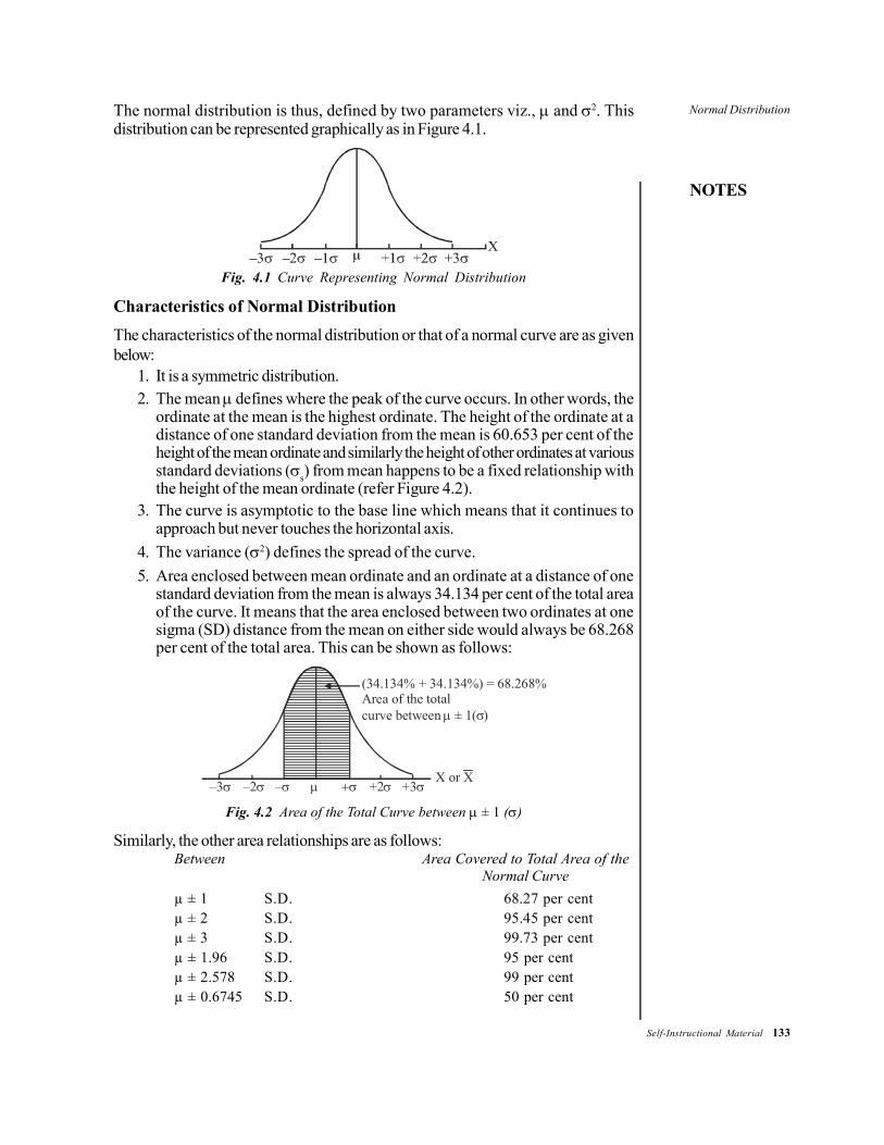
Normal Distribution
NOTES
Self-Instructional Material 133
The normal distribution is thus, defined by two parameters viz., µ and σ2. Thisdistribution can be represented graphically as in Figure 4.1.
Fig. 4.1 Curve Representing Normal Distribution
Characteristics of Normal DistributionThe characteristics of the normal distribution or that of a normal curve are as givenbelow:
1. It is a symmetric distribution.2. The mean µ defines where the peak of the curve occurs. In other words, the
ordinate at the mean is the highest ordinate. The height of the ordinate at adistance of one standard deviation from the mean is 60.653 per cent of theheight of the mean ordinate and similarly the height of other ordinates at variousstandard deviations (σs) from mean happens to be a fixed relationship withthe height of the mean ordinate (refer Figure 4.2).
3. The curve is asymptotic to the base line which means that it continues toapproach but never touches the horizontal axis.
4. The variance (σ2) defines the spread of the curve.5. Area enclosed between mean ordinate and an ordinate at a distance of one
standard deviation from the mean is always 34.134 per cent of the total areaof the curve. It means that the area enclosed between two ordinates at onesigma (SD) distance from the mean on either side would always be 68.268per cent of the total area. This can be shown as follows:
–3σ –2σ –σ µ +σ +2σ +3σX or X
(34.134% + 34.134%) = 68.268%Area of the totalcurve between ± 1( )µ σ
Fig. 4.2 Area of the Total Curve between µ ± 1 (σ)
Similarly, the other area relationships are as follows:Between Area Covered to Total Area of the
Normal Curveµ ± 1 S.D. 68.27 per centµ ± 2 S.D. 95.45 per centµ ± 3 S.D. 99.73 per centµ ± 1.96 S.D. 95 per centµ ± 2.578 S.D. 99 per centµ ± 0.6745 S.D. 50 per cent

134 Self-Instructional Material
Normal Distribution
NOTES
6. The normal distribution has only one mode since the curve has a single peak.In other words, it is always a unimodal distribution.
7. The maximum ordinate divides the graph of normal curve into two equal parts.8. In addition to all the above stated characteristics the curve has the following
properties:
(a) µ = x_
(b) µ2= σ2 = Variance(c) µ4=3σ4
(d) Moment Coefficient of Kurtosis = 3
Family of Normal DistributionsWe can have several normal probability distributions but each particular normaldistribution is being defined by its two parameters viz., the mean (µ) and the standarddeviation (σ). There is, thus, not a single normal curve but rather a family of normalcurves (refer Figure 4.3). We can exhibit some of these as under:Normal curves with identical means but different standard deviations:
µ in a normaldistribution
Curve having small standarddeviation say ( = 1)σCurve having large standarddeviation say ( = 5)σCurve having very large standarddeviation say ( = 10)σ
Normal curves with identical standard deviation but each with different means:
Normal curves each with different standard deviations and different means:
Fig. 4.3 Family of Curves

Normal Distribution
NOTES
Self-Instructional Material 135
How to Measure the Area under the Normal CurveWe have stated above some of the area relationships involving certain intervals ofstandard deviations (plus and minus) from the means that are true in case of anormal curve. But what should be done in all other cases? We can make use of thestatistical tables constructed by mathematicians for the purpose. Using these tableswe can find the area (or probability, taking the entire area of the curve as equal to 1)that the normally distributed random variable will lie within certain distances fromthe mean. These distances are defined in terms of standard deviations. While usingthe tables showing the area under the normal curve we talk in terms of standardvariate (symbolically Z ) which really means standard deviations without units ofmeasurement and this ‘Z’ is worked out as under:
μσ
XZ −=
Where, Z = The standard variate (or number of standard deviations from X to themean of the distribution).
X = Value of the random variable under consideration.µ = Mean of the distribution of the random variable.σ = Standard deviation of the distribution.
The table showing the area under the normal curve (often termed as the standardnormal probability distribution table) is organized in terms of standard variate (or Z)values. It gives the values for only half the area under the normal curve, beginningwith Z = 0 at the mean. Since the normal distribution is perfectly symmetrical thevalues true for one half of the curve are also true for the other half. We nowillustrate the use of such a table for working out certain problems.Example 4.1: A banker claims that the life of a regular savings account openedwith his bank averages 18 months with a standard deviation of 6.45 months. Answerthe following: (a) What is the probability that there will still be money in 22 months ina savings account opened with the said bank by a depositor? (b) What is the probabilitythat the account will have been closed before two years?Solution: (a) For finding the required probability we are interested in the area of theportion of the normal curve as shaded and shown in figure given below:
σ = 6.45
μ = 18z = 0 X = 22
Let us calculate Z as under:
Z =μ 22 18 0.62
σ 6.45X − −
= =

136 Self-Instructional Material
Normal Distribution
NOTES
The value from the table showing the area under the normal curve for Z = 0.62 is0.2324. This means that the area of the curve between µ = 18 and X = 22 is 0.2324.Hence, the area of the shaded portion of the curve is (0.5) – (0.2324) = 0.2676 sincethe area of the entire right hand portion of the curve always happens to be 0.5. Thus,the probability that there will still be money in 22 months in a savings account is0.2676.(b) For finding the required probability we are interested in the area of the portion
of the normal curve as shaded and shown in figure given below:
σ = 6.45
μ = 18z = 0 X = 24
For the purpose we calculate,24 18 0.93
6.45Z
The value from the concerning table, when Z = 0.93, is 0.3238 which refers to thearea of the curve between µ = 18 and X = 24. The area of the entire left hand portionof the curve is 0.5 as usual.Hence, the area of the shaded portion is (0.5) + (0.3238) = 0.8238 which is therequired probability that the account will have been closed before two years, i.e.,before 24 months.Example 4.2: Regarding a certain normal distribution concerning the income of theindividuals we are given that mean=500 rupees and standard deviation =100 rupees.Find the probability that an individual selected at random will belong to income group,
(a) 550 to 650 (b) 420 to 570Solution: (a) For finding the required probability we are interested in the area of theportion of the normal curve as shaded and shown below:
= 100
= 500µ = 500 X = 650z = 0 X = 550

Normal Distribution
NOTES
Self-Instructional Material 137
For finding the area of the curve between X = 550 to 650, let us do the followingcalculations:
550 500 50 0.50100 100
Z −= = =
Corresponding to which the area between µ = 500 and X = 550 in the curve as pertable is equal to 0.1915 and,
650 500 150 1.5100 100
Z
Corresponding to which, the area between µ = 500 and X = 650 in the curve, as pertable, is equal to 0.4332.Hence, the area of the curve that lies between X = 550 and X = 650 is,
(0.4332) – (0.1915) = 0.2417This is the required probability that an individual selected at random will belong toincome group of 550 to 650.(b) For finding the required probability we are interested in the area of the portionof the normal curve as shaded and shown below:To find the area of the shaded portion we make the following calculations:
= 100
= 100z = 0z = 0
X = 420 X = 570
570 500 0.70100
Z −= =
Corresponding to which the area between µ = 500 and X = 570 in the curve as pertable is equal to 0.2580.
and 420 500 0.80100
Z −= = −
Corresponding to which the area between µ = 500 and X = 420 in the curve as pertable is equal to 0.2881.
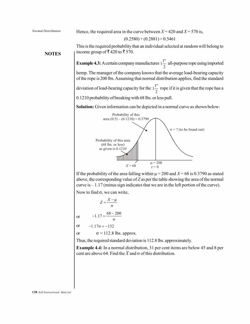
138 Self-Instructional Material
Normal Distribution
NOTES
Hence, the required area in the curve between X = 420 and X = 570 is,(0.2580) + (0.2881) = 0.5461
This is the required probability that an individual selected at random will belong toincome group of 420 to 570.
Example 4.3: A certain company manufactures 112'' all-purpose rope using imported
hemp. The manager of the company knows that the average load-bearing capacityof the rope is 200 lbs. Assuming that normal distribution applies, find the standard
deviation of load-bearing capacity for the 112'' rope if it is given that the rope has a
0.1210 probability of breaking with 68 lbs. or less pull.
Solution: Given information can be depicted in a normal curve as shown below:
μ = 200X = 68 z = 0
σ = ? (to be found out)
Probability of thisarea (0.5) – (0.1210) = 0.3790
Probability of this area(68 lbs. or less)
as given is 0.1210
If the probability of the area falling within µ = 200 and X = 68 is 0.3790 as statedabove, the corresponding value of Z as per the table showing the area of the normalcurve is – 1.17 (minus sign indicates that we are in the left portion of the curve).Now to find σ, we can write,
μ
σXZ −
=
or68 2001.17
σ−
− =
or 1.17σ 132− = −
or σ = 112.8 lbs. approx.Thus, the required standard deviation is 112.8 lbs. approximately.Example 4.4: In a normal distribution, 31 per cent items are below 45 and 8 percent are above 64. Find the X
_ and σ of this distribution.

Normal Distribution
NOTES
Self-Instructional Material 139
Solution: We can depict the given information in a normal curve as shown below:
X
X
X
X
If the probability of the area falling within µ and X = 45 is 0.19 as stated above, thecorresponding value of Z from the table showing the area of the normal curve is –0.50. Since, we are in the left portion of the curve, we can express this as under,
45 μ0.50σ−
− = (1)
Similarly, if the probability of the area falling within µ and X = 64 is 0.42, as statedabove, the corresponding value of Z from the area table is, +1.41. Since, we are inthe right portion of the curve we can express this as under,
64 μ1.41σ−
= (2)
If we solve Equations (1) and (2) above to obtain the value of µ or X , we have,− 0.5 σ = 45 – µ (3)1.41 σ = 64 – µ (4)
By subtracting Equation (4) from Equation (3) we have,− 1.91 σ = –19
∴ σ = 10
Putting σ = 10 in Equation (3) we have,− 5 = 45 – µ
∴ µ = 50
Hence, X_ (or µ)=50 and σ =10 for the concerning normal distribution.
Applications of Normal DistributionThe following are the applications of normal distribution:
1. Random processes: Many naturally occurring random processes tend tohave a distribution that is approximately normal. Examples can be found inany field, these include: SAT test scores of college bound students and bodytemperature of a healthy adult.

140 Self-Instructional Material
Normal Distribution
NOTES
2. Approximation of binomial distribution: When np>5 and n(1–p)>5, thenormal distribution provides a good approximation of the binomial distribution.Distributions that are based on multiple observations, for example the Binomialdistribution, approach the normal distribution when n gets large. The value n>30 is usually considered large.
3. Standardization: It is used where it is usually hypothesized that the theoreticaldistribution of a certain variable is normal, whereas the measurement of suchvariable may not give a normal distribution.For example, in the introductory classes of Statistics there are 200 studentsand it has been assumed that the performance of all the students in theexamination should be normally distributed. In addition, for giving reasonabledistribution of marks, the mean should be 55 and the standard deviation shouldbe 10. After the examinations being over, the lecturer marked all the papers,and the mean and standard deviation of the raw scores given by the lecturerare 50 and 6, respectively. For converting the raw score to standardize score,the following steps were taken:
(a) The standard score is obtained by Z= (X-50)/6.(b) Then the converted (standardized) = 10(Z) + 55.
Hence, a raw score of 56 will be converted into 65.4. Composite scores: When more than one measure is used to measure a
variable, the distribution of each measure usually differs from each other. Inorder to obtain an unbiased measure using several different measurements,each sub-measure is standardized before added together.For example, if the marks are awarded according to the average of the marksgiven by the Marker I and Marker II, then clearly the final grades are greatlyaffected by the Marker I than by Marker II as Marker I is awarded themarks with higher standard deviation as shown in table below:
For computing the composite score, the standardized scores of Marker I andMarker II should be averaged. If the ideal average score (µ) and standarddeviation (σ) is taken to be 60 and 10, respectively, then the Z scores isconverted into the standard score for each marker. The following table showsthe resulted average standardized score 60 for every student.

Normal Distribution
NOTES
Self-Instructional Material 141
5. Probability distribution: The probability distribution of X for large n is thenormal distribution. The Central Limit Theorem states that if the observationsare independent for one population which has a mean (µ) and standard deviation(σ) then for large n (n>30) X has a normal distribution with the same meanand a standard deviation of σ / √n.
4.2.1 Normal Probability Curve and its Uses
The Normal Probability Curve (NPC), simply known as normal curve, is a symmetricalbell-shaped curve. This curve is based upon the law of probability and discovered byFrench mathematician Abraham Demoivre (1667–1754) in the 18th century. In thiscurve, the mean, median and mode lie at the middle point of the distribution. Thetotal area of the curve represents the total number of cases and the middle pointrepresents the mean, median and mode. The base line is divided into six sigma units(σ units). The scores more than the mean come on the + σ side and the scores lessthan the mean come on the – σ side. The mean point (middle point) is marked aszero (0). All the scores are expected to lie between – 3σ to + 3σ.
Characteristics of Normal Probability CurveThe NPC or Normal Probability Curve has several features which are essential tounderstand for its use. The major characteristics are limited. They are as follows:
• It is a bell shaped curve.• The measures of central tendency are equal, i.e, mean, mode and median
concentrate on one point.• The height of the curve is 0.3989.• It is an asymptotic curve. The ends of the curve approach but never touch
the X-axis at the extremes because of the possibility of locating in the population,in cases where scores are still higher than our highest score or lower than ourlowest score. Therefore theoretically, it extends from minus infinity to plusinfinity as illustrated in Figure 4.4. Here, M is the mean or expectation (locationof the peak) and σ is the standard deviation.

142 Self-Instructional Material
Normal Distribution
NOTES
Fig. 4.4 Normal Curve Showing Areas at Different Distances from the Mean
• It has 50 per cent frequency above and 50 per cent below the mean. Themean is zero and it is always reference point.
• Standard deviation of a normal curve is always 1.• The points of inflection of the curve occur at points –1 unit above and below
mean.• The distribution of frequency per cent has the definite limits.• There is a definite relation between quartile deviation and standard deviation
in a normal distribution curve.• It is a mathematical curve and is an open-ended curve.
Some limits are as follows:• The middle 68 per cent frequency is between –1 and +1.• The middle 95 per cent frequency is between –1.96 and + 1.96.• The middle 99 per cent frequency is between –2.58 and + 2.58.
The total area under the normal curve is arbitrarily taken as 10,000. Every scoreshould be converted into standard score (Z score) by using the following formula:
X MZ −=
σ
The area in proportion should be converted into a percentage at the time ofreading the table. From the table, we can see the areas from mean to σ and also wecan read the value of σ scores from the mean for the corresponding fractional area.
4.2.2 Uses of Normal Probability Curve: ComputingPercentiles and Percentile Ranks
The uses of normal probability curve are discussed in this section.

Normal Distribution
NOTES
Self-Instructional Material 143
NPC is used to Determine the Percentage of Cases within Given Limits
Example 4.5: Given a distribution of scores with a mean of 15 and a standarddeviation of 5, what percentage of cases lie between 18 and 25 refer to figure givenbelow to calculate the answer.
(18-25) 25.15%
-3σ -2σ -1σ 1σ 2σ 3σ 0 5 10 15 20 25 30
Solution: Both the raw scores (18 and 25) are to be converted into Z scores.
Z score of 18 =X M−
σ=
18 155−
=35
= 0.6σ
Z score of 25 =X M−
σ=
25 155−
=105
According to the table of area of a normal probability curve, the totalpercentage of cases lie between the mean and 0.6σ is 22.57. The percentage ofcases lie between the mean and 2σ is 47.72. So, the total percentage of cases thatfall between the scores 18 and 25 is 47.72 – 22.57 = 25.15.
NPC is used to Determine the Limit which Includes a GivenPercentage of Cases
Example 4.6: Given a distribution of scores with a mean of 12 and an σ of 6, whatlimits will include the middle 70 per cent of the cases? Refer to figure given tocalculate the answer.

144 Self-Instructional Material
Normal Distribution
NOTES
70%
35% 35%
-3σ -2σ -1σ mean 1σ 2σ 3σ
Mean = 12, σ = 6 Solution: The middle 70 per cent of the cases in a normal distribution signifies that35 per cent cases above the mean and also 35 per cent cases below the mean.According to the table of area under NPC, 35 per cent of cases fall between themean and 1.04 σ. So the middle 70 per cent of the cases will lie between –1.04σ to+ 1.04σ.
The value of 1 σ = 6So 1.04 σ = 6 × 1.04 = 6.24The value of mean = 12So the lowest limit for the middle 70 per cent cases of the distribution is:12 – 6.24 = 5.76.The highest limit for the middle 70 per cent cases of the distribution is:12 + 6.24 = 18.24.Thus, the middle 70 per cent cases lie in between 5.76 and 18.24.
NPC is used to Determine the Percentile Rank of a Student in hisClass
Example 4.7: The score of a student in a class test is 70. The mean for the wholeclass is 50 and the σ is 10. Find the percentile rank of the student in the class. Referthe figure given below to find the answer.
M=50 S D= 10 97.72-PR -3σ -2σ -1σ 1σ 2σ 3σ 20 30 40 60 70 80

Normal Distribution
NOTES
Self-Instructional Material 145
Solution: The Z score for the score 70 is 70 50 2
10−
= σ
As per the table of area under the NPC, the area of the curve that liesbetween mean and 2σ is 47.72 per cent. The total percentage of cases below 70 is:
50 + 47.72 = 97.72 per cent or 98 per cent.Thus, the percentile rank of the student is 98.
NPC is used to Find out the Percentile Value of a Student whose PercentileRank is Known
Example 4.8: The percentile rank of a student in a class test is 80. The mean of theclass in the test is 50 and the σ is 20. Calculate the student’s score in the class test.Figure given below illustrates the case.
80% M=50 SD=20 50% 30% Score = 66.8 -3σ -2σ -1σ 84σ 1σ 2σ 3σ
Solution: The student has scored 30 per cent scores above the mean. According tothe table of area under NPC, 30 per cent cases from the mean is 0.84σ.
1σ = 20.0.84σ = 20 × .84 = 16.8Thus, the percentile value of the student is 50 + 16.8 = 66.8.
NPC is used to Divide a Group into Sub-Groups According totheir Capacity
Example 4.9: Suppose there is a group of 100 students in a Commerce class. Wewant to divide them into five small groups A, B, C, D and E according to their ability,the range of ability being equal in each sub-group. Find out how many studentsshould be placed in each category.

146 Self-Instructional Material
Normal Distribution
NOTES
C D B
E A
-3σ -1.8σ -.6σ Mean .6σ 1.8σ 3σ Solution: The total area under NPC is –3σ to + 3σ, that is 6σ. This 6σ should bedivided into five parts, so 6σ ÷ 5 = 1.2σ.
According to the table of area under NPC:3.5 per cent of the cases lie between 1.8 σ to 3σ (Group A, the high scorers).
23.8 per cent of the cases lie between .6σ to 1.8σ (23.8 per cent of the cases for Band also 23.8 per cent of the cases for D), the middle 45 per cent of the cases lie –0.6σ to + 0.6σ (Group C), and the lowest 3.5 per cent of the cases lie between –3σto – 1.8σ (Group E)
In category ‘A’ the number of students = 3.5 per cent = 3 or 4 students.In category ‘B’ the number of students = 23.8 per cent = 24 students.In category ‘C’ the number of students = 45 per cent = 45 students.In category ‘D’ the number of students = 23.8 per cent = 24 students.In category ‘E’ the number of students = 3.5 per cent = 3 or 4 students.
NPC is used to Compare the Scores of Students in Two Different Tests
Example 4.10: Suppose, a student scored 60 marks in English test and 80 marks instatistics test. The mean and SD for the English test is 30 and 10 respectively,whereas for the statistics test the mean is 70 and SD is 10. Find out, in which subjectthe student performed better. Refer to Figure given below. -3σ -2σ -1σ 1σ 2σ 3σ -3σ -2σ -1σ 1σ 2σ 3σ 0 10 20 40 50 60 40 50 60 80 90 100 M = 30 Mean = 70 SD = 10 SD = 10 English Test Statistics Test

Normal Distribution
NOTES
Self-Instructional Material 147
Solution: In case of the English test:Raw score = 60Mean = 30SD =10
So Z score for the English test = X M 60 30 30 3
10 10− −
= = = σσ
In case of statistics test raw score = 80Mean = 70SD = 10
So Z Score for the statistics test = X M 80 70 10 1
10 10− −
= = = σσ
So, the student has done better in the English than the statistics on.
NPC is Used to Determine the Relative Difficulty Level of Test Items
Example 4.11: In a standardized test of psychology, question numbers A, B, C andD were solved by the students, 45 per cent, 38 per cent, 30 per cent and 15 per centrespectively. Assuming the normality, find out the relative difficulty level of thequestions. Also explain the difficulty levels of questions. Table given below displaysthe information in tabular form.Solution:
Determining the Difficulty Level of Test Items
Question Number
Percentage of Successful Students
Percentage of Unsuccessful Students
Percentage distance of Mean of Unsuccessful Students
Difficulty Level
A 45 55 55-50=5 0.13σ B 38 62 62-50=12 0.31σ C 30 70 70-50=20 0.52σ D 15 85 85-50=35 1.04σ As we know that in an NPC, 50 – 50 cases lie both the sides of mean. The
mean of NPC is that point which is shown as 0. In an NPC, the explanation ofdifficulty level is done on the basis of σ — distance. Therefore, if a question is at thepositive side of the NPC and σ has more distance from the mean, the question of atest will be much difficult. The relative difficulty value of the test items has beenshown:
The questionA to B is 0.18σ is more difficult (0.31σ –0.13σ = 0.18σ)A to C is 0.39σ is more difficult (0.52σ –0.13σ = 0.39σ)A to D is 0.91σ is more difficult (1.04σ –0.13σ = 0.91σ)

148 Self-Instructional Material
Normal Distribution
NOTES
B to C is 0.21σ is more difficult (0.52σ –0.31σ = 0.21σ)B to D is 0.73σ is more difficult (1.04σ –0.31σ = 0.73σ)C to D is 0.52σ is more difficult (1.04σ –0.152σ = 0.52σ)
CHECK YOUR PROGRESS
1. List any three characteristics of normal distribution.2. What is a Normal Probability Curve?
4.3 NEED, IMPORTANCE AND SIGNIFICANCE OFTHE DIFFERENCE BETWEEN MEANS ANDOTHER STATISTICS
A statistical hypothesis is a statement about a population parameter. The statementis tentative in the sense that it carries some belief or involves an assumption thatmay or may not be found valid on verification. The act of verification consists oftesting the validity of belief(s) or examining the veracity of the assumption(s), whichis indeed what we do in testing hypotheses. When this is done on the basis of sampleevidence, testing is called statistical testing, and the hypothesis tested is known asstatistical hypothesis.
4.3.1 Null Hypothesis
A statistical hypothesis stated with a view to testing its validity is in fact a nullhypothesis and is known as such. It is always the null hypothesis, denoted as H0,that is tested on the basis of sample information.
As the sample information may or may not be found consistent with thestated hypothesis, it is important to note the following:
(a) If the information is found inconsistent with H0, the null hypothesis isrejected and we conclude that it is false. On the contrary, if the sampleinformation is found consistent with H0, it is accepted even though wedo not conclude that it is true.
(b) The reason for accepting H0 and yet not concluding that it is true, is thatthe sample information that justifies acceptance of H0 is not sufficientto conclude that it is indeed true. When sample information supportsH0, it can at best be considered adequate to conclude that H0 is notfalse.
The interpretation in b) above has a direct bearing on how the null hypothesisis to be stated. This requires that the hypothesis is stated with a view to rejecting it.For, in the event of the sample information being inconsistent with the statedhypothesis, it is safer to conclude that the hypothesis is false and be rejected. Thisprecisely is the reason why the hypothesis to be tested is called the null hypothesis.

Normal Distribution
NOTES
Self-Instructional Material 149
And, it is in this sense that testing essentially means testing a null hypothesis, whichis stated specifically with a view to be rejected.
Alternative HypothesisRejection of H0 implies that it is rejected in favour of some other hypothesis beingaccepted. A hypothesis that comes to be accepted at the cost of H0 is called thealternative hypothesis. Denoted as H1 it may be stated in different ways dependingon the nature of the problem statement.
If the hypothesis to be tested relates to any parameter Θ whose value ispredetermined or otherwise specified as, say, Θ = 60 units, the null hypothesis isstated as
H0 : Θ = 60 units.The form in which H1 is to be stated depends on our what the present value
of Θ is expected to be.The alternative hypothesis H1 may thus be stated in keeping with either of
the following two situations:1. In a problem situation where our interest is limited to knowing whether
the value of Θ is the same as before or has changed, the alternativehypothesis is stated asH1: Θ ≠ 60 units.The value of Θ = 60 units in H0 known as the hypothesised value. It isdenoted as Θ0, so that H0 may be stated asH0 : Θ ≠ Θ0
and the alternative hypothesis asH1 : Θ ≠ Θ0,where Θ0 = 60 units.
2. In the same or a different problem situation, our interest may be toknow if the value of Θ has increased or decreased compared to thehypothesised value Θ0. Where Θ is expected to have increased, thenull hypothesisH0 : Θ = Θ0
is tested against the alternative hypothesisH1 : Θ > Θ0.On the contrary, where Θ is expected to have decreased the nullhypothesis H0 is tested against the alternative hypothesisH1 : Θ < Θ0.
Thus, in effect, there are three different ways of stating H1. In each case,statistical testing means testing H0 against H1. It essentially involves a two-choicetesting in as much as it results either in the rejection of H0 in favour of H1, or in theacceptance of H0 against H1.

150 Self-Instructional Material
Normal Distribution
NOTES
The various points that emerge from the above discussion may thus besummarised and restated as follows:
• A statistical hypothesis, often called a null hypothesis H0, is tested againstan alternative hypothesis H1. The latter can be stated in different waysdepending on the problem situation as to what the parameter is expectedto be at a given point of time.
• A statistical hypothesis is stated with reference to a population parameter,never in relation to the corresponding sample statistic. The appropriatesample statistic serves merely as a means, by providing a point estimate,to decide whether a statistical hypothesis is to be rejected or accepted.
• A statistical hypothesis is always stated in the present tense in a mannerthat some general state of affairs currently exists. Use of future tense instating a hypothesis is not admissible, as in that case the null hypothesiswill involve a future state of affairs about something that may not exist.
4.3.2 Z-test
The Z-test is any statistical test for which the distribution of the test statistic underthe null hypothesis can be approximated by means of a normal distribution. Typically,it is a statistical test used to determine whether two population means are differentwhen the variances are known and the sample size is large. The test statistic isassumed to have a normal distribution and parameters, such as standard deviationshould be known in order for an accurate Z-test to be performed. Because of theCentral Limit Theorem (CLT), many test statistics are approximately normallydistributed for large samples.
For each significance level, the Z-test has a single critical value. Consequently,several statistical tests can be easily performed as approximation of Z-tests if thesample size is large or the population variance is known. But if the population varianceis unknown and has to be estimated from the sample itself and the sample size is notlarge (n < 30) then the Student t-test may be more appropriate.
Formula for the Z-Score for a Single ValueZ-score can be calculated using the following formula:
xZ − µ=
σ
Where,x = Sample score.µ = Population mean.σ = Population standard deviation.The Z-score is the number of standard deviations which are away from the
mean and can be used to compare different scores when the mean and standarddeviation of the population are known. These comparisons are based on the

Normal Distribution
NOTES
Self-Instructional Material 151
assumptions that the distribution of the population is normal and that the two scoresare drawn from tests that measure the same construct(s).Example 4.12: Ram has taken tests a few weeks ago and got scores of 630 inVerbal and 700 in Quantitative. The means and standard deviations of a set of testtakers are as follows:
Verbal QuantitativeMean 469 591Standard Deviation 119 148
Calculate the Z-score of Ram for both the subject.Solution: The Z-score of Ram for both the subject is calculated as follows:Here,
Mean of verbal test = 469Standard deviation of verbal test = 119Sample score of verbal test = 630
Z-score for verbal test = 630 − 469 / 119
= 161 / 119= 1.35
Again,Mean of quantitative test = 591Standard deviation of quantitative test = 148Sample score of quantitative test = 700
Z-score for quantitative test = 700 − 591 / 148
= 109 / 148= 0.73
Example 4.13: Find the Z-score corresponding to a raw score of 132 from anormal distribution with mean 100 and standard deviation 15.Solution: The Z-score is calculated as follows:
Here,Raw score = 132Mean = 100Standard deviation =15
Z-score = 132 100 2.133
15−
=
Example 4.14: A Z-score of 1.7 was found from an observation coming from anormal distribution with mean 14 and standard deviation 3. Find the raw score.

152 Self-Instructional Material
Normal Distribution
NOTES
Solution: The raw score is obtained as follows:Here,Z-score = 1.7Mean = 14Standard deviation = 3Let the raw score be x.We know:
Z-Score=Mean
Standard Deviationx −
⇒ Ζ-Score × Standard Deviation = x − Mean⇒ 1.7 × 3 = x − 14⇒ 5.1 = x − 14⇒ 5.1 + 14 = x⇒ x = 19.1The raw score is 19.1.
Formula for Sample Mean using One Sample Z-TestOne sample Z-test can be calculated from the following formula:
z = ( μ)σ
x
n
−
Where,
x = Sample mean.µ = Specific value to be tested.σ = Population standard deviation.n = Size of the sample.
Example 4.15: A test is conducted for H0 where µ = 20, with σ = 4. A sample ofsize 36 has x = 21.4. Find the value of one sample Z-test.
Solution: The value of one sample Z-test is calculated as follows:Here,
x = 21.4µ = 20σ = 4n = 36Z = 21.4 – 20 / (4/√36)
= 1.4 / (4 / 6)

Normal Distribution
NOTES
Self-Instructional Material 153
= 1.4 / (2/3)= 3 × 1.4 / 2= 4.2 / 2= 2.1
The value of one sample Z-test is 2.1.
Z-Test for Independent and Dependent GroupA practical example is given below using the hypothesis testing to illustrate the Z-test for differences in proportions between two independent groups. The researchquestion for our example will be: Do a greater proportion of high school students inthe population smoke cigarettes in urban rather than rural cities? This is a directionalquestion. A step-by-step outline will be followed to test this research question.Step 1: The directional research question in a statistical hypothesis format shouldbe stated.
H0: P1≤ P2 (or P1– P2≤0)HA: P1> P2 (or P1– P2>0)
Here, ‘H’ stands for hypothesis with subscripts ‘0’ for the null statisticalhypothesis and ‘A’ for the alternative statistical hypothesis. The alternative statisticalhypothesis is stated to reflect the research question. In this example, the alternativestatistical hypothesis indicates the directional nature of the research question. Also,P1 is the population proportion of high school students who smokes in the urban citywhereas P2 is the population proportion of high school students who smoke in therural city.Step 2: The criteria for rejecting the null hypothesis and accepting the alternativehypothesis should be determined.
Given α = 0.1 level of significance, we select the corresponding Z valuewhich is the closest to1 per cent of the area under the normal curve. If ourcomputer Z-test statistics is greater than Z-value, we would reject the nullhypothesis. This establishes our region of rejection, R, or the probability areaunder the normal curve where differences in sample proportions are unlikely tooccur by random chance.Step 3: The sample data of the collected Z-test statistics should be computed.A random sample of 20 percent of all high school students from both urban and ruralcity was selected. In urban city, 20,000 high school students were sampled with25 per cent smoking cigarettes (n1 = 5,000). In the rural city, 1,000 high schoolstudents were sampled with 15 per cent smoking cigarette (n2=150). The proportionswere:
P1 = 25 (25 per cent of the boys in the sample of high school students smokingcigarettes).
P2 = 15 (15 per cent of the girls in the sample of high school students smokingcigarettes).

154 Self-Instructional Material
Normal Distribution
NOTES
The standard deviation of the sampling distribution of the difference inindependent sample proportions is called the standard error of the difference betweenindependent sample proportions. This value is needed to compute the Z-test statistics.The formula is as follows:
1 2P PpqSN− =
Where,p = (n1+ n2/N) = (5000 + 150/21,000) = 245.q = 1 – p = 1 – 245 = 755.n1 = Number in the first sample = 5,000.n2 = Number in the first sample = 150.N = Total sample size taken = (20,000 + 1000) = 21,000.
1 2
0.245(0.755) 0.00321000P PS − = =
The Z-test can now be computed as follows:
1 2
1 2 0.25 0.15 0.10 33.330.003 0.003P P
P PZS −
− −= = = =
Step 4: The confidence interval around the Z-test statistic should be computed.A confidence interval is computed by using the per cent difference between
the two independent groups (P1 – P2=0.10), the Z value corresponding to a givenalpha α level for a two-tailed region of region (Z = 2.58) and then the standarddeviation of the sampling distribution or standard error of the test statistics(SP1-P2
=0.003)CI99 = 0.10 +/ – (2.58) (0.003)CI99 = 0.10 +/ – (0.008)CI99 = (0.092, 0.108)
Step 5: The Z-test static results should be interpretedOur interception is based upon a test of the null hypothesis and a 99 per cent
confidence interval around the computed Z-test statistic. Since the computedZ = 33.33 is greater than the Z value, Z = 2.33 at the 0.1 level of significance, wereject the null statistical hypothesis in favor of alternative statistical hypothesis. Theprobability that the observed difference in the sample proportions of 10 per centwould have occurred by chance is less than 0.01. We can therefore conclude thatthe urban city had a greater percentage of high school students smoking cigarettesthan the rural city. The Type I error was set at 0.01, so that we can be fairlyconfident in our interception.

Normal Distribution
NOTES
Self-Instructional Material 155
The confidence interval was calculated as 0.92 to 0.108, indicating that wecan be 99 per cent confident that this interval contains the difference between thepopulation proportions from which the samples were taken. Moreover, thenarrowness of the confidence interval gives the idea that how much the differencein the independent sample proportions might vary from random sample to randomsample. Consequently, we can feel fairly confident that a 9 per cent (0.092) to11 per cent (0.108) difference would exist between urban and rural city highschool students smoking cigarettes upon repeated sampling of the population.
Z-Test for Dependent GroupThe null hypothesis that there is no difference between two population proportionscan also be tested for dependent samples using the Z-test statistics. The researchdesign would involve obtaining percentage from the same sample or group twice.The research design would therefore have paired observations. Some examples ofwhen this occurs would be:
1. Test differences in proportions of agreement in a group before and after adiscussion of the death penalty.
2. Test differences in per cent passing for students who take two similar tests.3. Test differences in proportion of the employee who support a retirement plan
and the proportion that support a company daycare.The research design involves studying the impact of diversity training on the
proportion of the company employees who would favor hiring foreign workers.Before and after diversity training, employees were asked whether or not they werein favor of company hiring foreign workers. A step-by-step approach to hypothesistesting will be used as follows:Step 1: The non-directional research question should be stated in the statisticalhypothesis format.
H0: P1 = P2 (or P1 – P2 = 0)HA: P1 ≠ P2 (or P1 – P2 ≠ 0)
Step 2: The criteria for rejecting the null hypothesis and accepting the alternativehypothesis should be determined.
Given α = 0.05, we select the corresponding Z value which is closest to 5 percent of the area under the normal curve (2.5 per cent in each tail of the normalcurve). If our computed Z-test statistics is greater that this Z value, we would rejectthe null hypothesis and accept the alternative hypothesis. This establishes our regionof rejection R or the probability areas under the normal curve where differences insample proportions are unlikely to occur by random chance.
R: Z ± 1.96Step 3: The sample data should be collected and the Z-test statistics should becomputed.
A random sample of 100 employees from a high-tech company wereinterviewed before and after a diversity training session and asked whether or not

156 Self-Instructional Material
Normal Distribution
NOTES
they favored the company hiring foreign workers. Their samples responses were asfollows:
No YesAfter Diversity Training Yes 10(0.10) 20(0.20) 30(0.30)BeforeDiversity Training No 50(0.50) 20(0.20) 70(0.70)
Total 60(0.60) 40(0.40) 100The standard deviation of the sampling distribution of the differences in
dependent sample proportion is called standard error of the difference betweendependent sample proportions. This value is needed to compute the Z-test statistics.The formula is:
1 2
11 22P P
P PN
S −+
=
Where,P11 = Percent change from before to after training (Yes → No) = 0.10P12 = Percent change from before to after training (No → Yes) = 0.20N = Total sample size =100
1 2
1 2 0.30 0.40 0.10 1.820.055 0.055P P
P PZS −
− − −= = = = −
Step 4: The confidence interval around the Z-test statistics should be computed.Step 5: The Z-test statistics result should be interpreted.
4.3.3 t-Test
Sir William S. Gosset (pen name Student) developed a significance test and throughit made a significant contribution to the theory of sampling applicable in case ofsmall samples. When population variance is not known, the test is commonly knownas Student’s t-test and is based on the t distribution.
Like normal distribution, t distribution is also symmetrical but happens to beflatter than normal distribution. Moreover, there is a different t distribution for everypossible sample size. As the sample size gets larger, the shape of the t distributionloses its flatness and becomes approximately equal to the normal distribution. Infact, for sample sizes of more than 30, the t distribution is so close to the normaldistribution that we will use the normal to approximate the t distribution. Thus, whenn is small, the t distribution is far from normal, but when n is infinite, it is identical tonormal distribution.
For applying t-test in context of small samples, the t value is calculated firstof all and then the calculated value is compared with the table value of t at certain

Normal Distribution
NOTES
Self-Instructional Material 157
level of significance for given degrees of freedom. If the calculated value of texceeds the table value (say t0.05), we infer that the difference is significant at5 per cent level but if calculated value is t0 is less than its concerning table value,the difference is not treated as significant.The t-test is used when two conditions are fullfiled,
(a) The sample size is less than 30, i.e., when 30.n ≤ .(b) The population standard deviation (σp) must be unknown.
In using the t-test, we assume the following:(a) That the population is normal or approximately normal.(b) That the observations are independent and the samples are randomly drawn
samples.(c) That there is no measurement error.(d) That in the case of two samples, population variances are regarded as equal
if equality of the two population means is to be tested.The following formulae are commonly used to calculate the t value:
(a) To Test the Significance of the Mean of a Random Sample
| || x
XtS SE X
− µ=
Where, X = Mean of the sample
µ = Mean of the universe
XSE = S.E. of mean in case of small sample and is worked out as follows:
2( )i
sX
X XnSE
n n
Σ −σ
= =
and the degrees of freedom = (n – 1).The above stated formula for t can as well be stated as under:
| |
X
XtSE
− µ=
2
| |( )
1
XX Xn
n
−µ=
Σ −−
2
| | =( )
1
X nX Xn
− µ×
Σ −−
If we want to work out the probable or fiducial limits of population mean (µ)in case of small samples, we can use either of the following:
(a) Probable limits with 95 per cent confidence level:
0.05 ( )XX SE tµ = ±
(b) Probable limits with 99 per cent confidence level:
0.01 ( )XX SE tµ = ±

158 Self-Instructional Material
Normal Distribution
NOTES
At other confidence levels, the limits can be worked out in a similar manner,taking the concerning table value of t just as we have taken t0.05 in (a) and t0.01 in(b) above.(b) To Test the Difference between the Means of the Two Samples
1 2
1 2| |SE X X
X Xt−
−=
Where, 1X = Mean of the Sample 1.
2X = Mean of the Sample 2.
1 2X XSE − = Standard Error of difference between two sample means and isworked out as follows:
1 2
221 1 2 2
1 2
1 2
( ) ( )2
1 1
i iX X
X X X XSE
n n
n n
−
− + −=
+ −
× +
∑ ∑
and the degrees of freedom = (n1 + n2 – 2).When the actual means are in fraction, then use of assumed means is
convenient. In such a case, the standard deviation of difference, i.e.,
2 21 1 2 2
1 2
( ) + ( )2
i iX X X Xn n
Σ + Σ −+ −
can be worked out by the following short-cut formula:
2 2 2 21 1 2 1 1 1 2 2 2 2
1 2
( ) ( ) ( ) ( )2
i i i iX A X A n X A n X An n
Σ − + Σ − − − − −=
+ −
Where, A1 = Assumed mean of Sample 1.A2 = Assumed mean of Sample 2.X1 = True mean of Sample 1.X2 = True mean of Sample 2.
(c) To Test the Significance of an Observed Correlation Coefficient
22
1rt n
r= × −
−
Here, t is based on (n – 2) degrees of freedom.
(d) To Test and Compare Sample MeanThe t-test can be used to compare a sample mean to an accepted value (of apopulation mean) or it can be used to compare the means of two sample sets.

Normal Distribution
NOTES
Self-Instructional Material 159
t-Test to Compare One Sample Mean to an Accepted ValueThe formula for the calculation of the t-statistic for one sample mean is as follows:
0μ/
xts n
−=
Here, s is the standard deviation of the sample and not the population standarddeviation.
t-Test to Compare Two Sample MeansThe method for comparing two sample means is very similar. The only two differencesare the equation used to compute the t-statistic and the degrees of freedom forchoosing the tabulate t-value. The formula is given as follows:
1 2
2 21 2
1 2
x xts sn n
−=
+
In this case, we require two separate sample means, standard deviations andsample size. The formula for degrees of freedom (df) depends on the condition.
One-sample t-test: df = n – 1
Two-sample t-test: df =
22 21 2
1 22 22 2
1 2
1 2
1 21 1
s sn n
s sn n
n n
+
+
− −
Example 4.16 A one sample t-test is conducted on H0: µ = 81.6. The sample hasx = 84.1, s = 3.1 and n = 25. Find the t-test statistics.
Solution: The t-test statistics is obtained as follows:
x = 84.1µ = 81.6s = 3.1n = 25
t 0μ/
xs n
−=
= 84.1 – 81.6 / (3.1 / √ 25)= 2.5 / (3.1 / 5)= 2.5 / 0.62= 4.032
The value of t as per t-test statistics is 4.032.

160 Self-Instructional Material
Normal Distribution
NOTES
Example 4.17: Two random samples have been selected and a two sample t-testfor the difference in population means is conducted with H0: µ1 = µ2 vs. Ha: µ1 > µ2.The results are s1 = 2.5, 1x = 9.7, n1 = 30, s2 = 2.9, 2x = 9.1 and n2 = 35. What is thevalue of t-test?Solution: The value of t-test is obtained as follows:Here,
1x = 9.7
2x = 9.1
n1 = 30n2 = 35s1 = 2.5s2 = 2.9
We know:
t 1 22 21 2
1 2
x xs sn n
−=
+
= 9.7 – 9.1 / √ (2.5)2/30 + (2.9)2 / 35= 0.6 / √6.25/ 30 + 8.41/35= 0.6 / √ 0.208 + 0.240
= 0.6 / 0.448 = 0.6 / 0.66 = 0.90
The value of t as per as per t-test statistics is 0.90.Example 4.18: Comparison of the birth weights of new born babies of women whoparticipated in an intervention with the birth weights of a group that did not participateare given below.
Participated Not Participated Average Weight 3100 gm 2750 gm SD 420 425 n 75 75 Calculate the value of t using t-test.
Solution: The value of t-test is calculated as follows:Here,
1x = 3100
2x = 2750

Normal Distribution
NOTES
Self-Instructional Material 161
SD1 = 420SD2= 425n1 = 75n2 = 75
Now the value of t can be calculated as follows:
t =
1 2
2 21 2
1 2
x x
SD SDn n
−
+
t =2 2
3100 2750
420 42575 75
−
+
t =350
2352 2408.3+
t = 5.07The value of t as per as per t-test statistics is 5.07.Example 4.19: A sample of 10 measurements of the diameter of a sphere, gave amean X = 4.38 inches and a standard deviation, σ = 0.06 inches. Find (a) 95 per centand (b) 99 per cent confidence limits for the actual diameter.Solution: On the basis of the given data the standard error of mean:
σ 0.06 0.06 0.0231 10 1
s
n= = = =
− −
Assuming the sample mean 4.38 inches to be the population mean, the requiredlimits are as follows:
(a) 95 per cent confidence limits = 0.05( )XX SE t± with degrees of freedom
= 4.38 ± .02(2.262)= 4.38 ± .04524
i.e., 4.335 to 4.425
(b) 99 per cent confidence limits = 0.01( )XX SE t± with 9 degrees of freedom
= 4.38 ± .02(3.25) = 4.38 ± .0650 i.e., 4.3150 to 4.4450.Example 4.20: It was found that the coefficient of correlation between two variablescalculated from a sample of 25 items was 0.37. Test the significance of r at 5 percent level with the help of t-test.

162 Self-Instructional Material
Normal Distribution
NOTES
Solution: To test the significance of r through t-test, we use the following formulafor calculating t value:
2
2
21
0.37 = 25 21 (0.37)
=1.903
rt nr
= × −−
× −−
Degrees of freedom = (n–2) = (25–2) = 23The table value of α at 5 per cent level of significance for 23 degrees of
freedom is 2.069 for a two-tailed test.The calculated value of t is less than its table value, hence r is insignificant.
t-Test for Independent and Dependent GroupUnder this heading, you will learn about t-Test for independent and dependent group.
Independent t-TestThe sampling distribution of the difference between the means of two independentsamples provides the basics for the testing of a mean difference hypothesis betweentwo groups.
A typical research in which one would use the independent t -test mightinvolve one group of employees receiving sales training and the second group ofemployees not receiving any sales training. The number of sales for each group isrecorded and averaged. The null hypothesis would be stated when the averagesales for the two groups are equal. The alternative hypothesis would be stated whenthe group receiving the sales training will on average have higher sales than thegroup that did not receive any sales training. If the sample data for the two groupswere recorded for Sales Training where the mean = 40, standard deviation= 10, n =100, then the independent t-test can be computed as follows:
1 2
1 2
X X
X XtS −
−=
Thus, the independent t-test can be computed as follows:
0 40 7.091.41
t 5 −= =
Dependent t-TestThe dependent t-test is sometimes referred to as the paired t-test because it usestwo sets of scores on the same individuals.
A typical research situation that uses the dependent t-test involves a reputedmeasure design with one group. For example, a psychologist is studying the effectof certain motion picture upon the attribute of violence. The psychologist hypothesesthat viewing the motion will cause the students attribute to be more violent. A random

Normal Distribution
NOTES
Self-Instructional Material 163
sample of 10 students is given an attribute towards violence inventory before viewingthe motion picture. Next 10 students view the motion picture which contains graphicviolence portrayed as acceptable behavior. The ten students are the given the attributetowards violence inventory after viewing the motion picture. The average attributetoward violence score for students before viewing the motion picture was 6.75, butafter viewing the motion picture it is 73. There are ten pairs of scores so ten scoredifferences are squared and summed to calculate the sum of square difference. Thestandard error of the dependent t-test is the square root of the sum of squaredifferences divide by N(N – 1).
The dependent t-test to investigate whether the student’s attribute towardsthe violence changed after viewing the motion picture would be calculated as follows:
D
DtS
=
The numerator in the above formula is the average difference between the post andpre means score on the attribute towards violence inventory which is 73 – 67.5 =5.5.The denominator is calculated as follows:
Student Pre Post D D2
1 67.5D = 2 73.0D = ΣD = 55 ΣD2 = 725
Thus the dependent t-test is calculated as t = 5.5/ 2.17=2.53
4.3.4 Sampling Distribution of Means
The sampling distribution of a statistic is the distribution of that specific statisticwhich is considered as a random variable when derived from a random sample ofsize n. It may be considered as the distribution of the statistic for all possiblesamples from the same population of a given size. Thus the sampling distributiondepends on the underlying distribution of the population, the statistic being considered,the sampling procedure employed and the sample size used.
The mean of the sampling distribution is the mean of the population fromwhich the scores were sampled. Therefore, if a population has a mean µ, then themean of the sampling distribution of the mean is also µ. We will discuss here thelarge samples and the small samples.

164 Self-Instructional Material
Normal Distribution
NOTES
Large SamplesAn important principle, known as the ‘Central Limit Theorem (CLT)’, describes thecharacteristics of sample means if a large number of equal-sized samples (greaterthan 30) are selected at random from an infinite population. The central limit theoremstates that, ‘Given a population with a finite mean µ and a finite non-zero varianceσ2, the sampling distribution of the mean approaches a normal distribution with amean of µ and a variance of σ2/N as N, the sample size, increases. The followingare some characteristic features of sample mean:
• The distribution of ‘sample means’ is normal and it possesses all thecharacteristics of a normal distribution.
• The average value of ‘sample means’ will be the same as the mean of thepopulation.
• The distribution of the ‘sample means’ around the population mean will haveits own standard deviation, known as ‘standard error of mean’, which isdenoted as SEM or σM. It is computed by the following formula:
M MSEN
σ= σ = (1)
Where, σ = Standard deviation of the population.N = The number of cases in the sample.
Since the value of σ (i.e., standard deviation of population) is usually notknown, we make an estimate of this standard error of mean by using the followingformula:
M Nσ
σ = (2)
Where, σ = Standard deviation of the sample.N = The number of cases in the sample.
To illustrate the use of Formula (2), let us assume that the mean of the attitudescores of a sample of 100 distance learners enrolled with Gauhati University towardsstudent support services is 25 and the standard deviation is 5. The standard error ofmean can be calculated accordingly:
M M5.0SE 0.50100
= σ = =
This ‘standard error of mean’ may be assumed as the standard deviation of adistribution of sample means, around the fixed population mean of all distance learners.In the case of large randomly selected samples, the sampling distribution of samplemeans is assumed to be normal.

Normal Distribution
NOTES
Self-Instructional Material 165
Fig. 4.5 Sampling Distribution of Means showing Variability of Obtained Meansaround the Population Mean in Terms of σM
The normal curve in Figure 4.5 shows that this sampling distribution is centredon the unknown population mean with standard deviation 0.50. The sample meansoften fall between the positive and the negative side of the population mean. About2/3 of our sample means (exactly 68.26 per cent) will lie within ± 1.00 σM of thepopulation mean, i.e., within a range of ±1 × 0.50 = ±0.50. Furthermore, 95 of our100 sample means will lie within ±2.00σM (more exactly ±1.96 σM) of the populationmean, i.e., 95 of 100 sample means will lie within ±1.96 × 0.50 or ±0.98 of thepopulation mean. In other words, the probability that our sample mean of 25 doesnot miss the population mean (MPop.) by more than ±0.98 is 0.95. Also, 99 of oursample means will be within ±3.00σM (more exactly ± 2.58 σM) of the populationmean. This indicates that 99 out of 100 sample means will fall within ± 2.58 × 0.50or ± 1.29 of the population mean. The probability (P) that our sample mean of 25does not miss the MPop. by more than ± 1.29 is 0.99.
Thus, the value of a population mean can be inferred from a randomly selectedsample mean and can be estimated on a probability basis.
4.3.5 Confidence Intervals and Levels of Significance
When we draw a large random sample from the population to obtain measures of avariable and compute the mean for the sample, we can use the ‘central limit theorem’and ‘normal probability curve’ to have an estimate of the population mean. We cansay that M has a 95 per cent chance of being within 1.96 standard error units ofMPop. In other words, a mean for a random sample has a chance of 95 per cent ofbeing within 1.96 σM units from MPop. It may also be said that there is a 99 per centchance that the sample mean lies within 2.58 σM units of M Pop. To be more specific,it may be stated that there is a 95 per cent probability that the limits M ± 1.96 σMenclose the population mean and the limits M ± 2.58 σM enclose the populationmean with 99 per cent probability. Such limits enclosing the population mean areknown as the ‘confidence intervals’.
These limits help us to adopt particularly two levels of confidence. One isknown as 5 per cent level or 0.05 levels and the other is known as 1 per cent level or0.01 level. The 0.05 level of confidence indicates that the probability MPop. that lieswithin the interval M±1.96 σM is 0.95 and that it falls outside of these limits is 0.05.

166 Self-Instructional Material
Normal Distribution
NOTES
By saying that probability is 0.99, it is meant that MPop. lies within the interval M±2.58 σM and that the probability of its falling outside of these limits is 0.01.
To illustrate, let us apply the concept to the previous problem. Taking as ourlimits M± 1.96 σM, we have 25 ±1.960 × 0.5 0 or a confidence interval marked offby the limits 24.02 and 25.98. Our confidence that this interval contains MPop. isexpressed by a probability of 0.95. If we want a higher degree of confidence, wecan take the 0.99 level of confidence for which the limits are M±2.58 σM or aconfidence interval given by the limits 23.71 and 26.29. We may be quite confidentthat MPop, is not lower than 23.71 nor higher than 26.29, i.e., the chances are 99 in100 that the MPop, lies between 23.71 and 26.19.Small SamplesWhen the number of cases in the sample is less than 30, we may estimate the valueof σM by the following formula:
MSE SN
= (3)
Where,S = Standard deviation of the small sample.N = The number of cases in the sample.The formula for computing S is as follows:
2
1xS
N∑
=−
(4)
Where,2x∑ = Sum of the squares of deviations of individual scores from the sample
mean.N = The number of cases in the sample.The concept of small size was developed by William Sealy Gosset, a consulting
statistician for Guinness Breweries of Dublin (Ireland) 1908. The principle is thatwe should not assume that the sampling distribution of means of small samples isnormally distributed. He found that the distribution curves of small sample meanswere somewhat different from the normal curve. When the size of the sample issmall then the t-distribution lies under the normal curve, but the tails or ends of thecurve are higher than the corresponding parts of the normal curve.
Degrees of FreedomWhile finding the standard deviation of small samples we use N–1 in the denominatorinstead of N in the basic formula for standard deviation. The difference in the twoformulae may seem very little, if N is sufficiently large. But there is a very importantdifference in the ‘meaning’ in the case of small samples. N–1 is known as the‘number of degrees of freedom’, denoted by ‘df’. The ‘number of degrees offreedom’ in a distribution is the number of observations or values that are independent
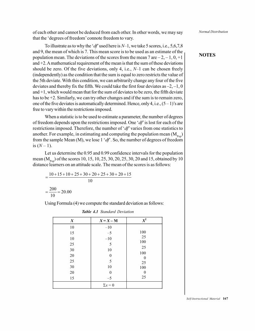
Normal Distribution
NOTES
Self-Instructional Material 167
of each other and cannot be deduced from each other. In other words, we may saythat the ‘degrees of freedom’ connote freedom to vary.
To illustrate as to why the ‘df’ used here is N–1, we take 5 scores, i.e., 5,6,7,8and 9, the mean of which is 7. This mean score is to be used as an estimate of thepopulation mean. The deviations of the scores from the mean 7 are – 2, – 1, 0, +1and +2. A mathematical requirement of the mean is that the sum of these deviationsshould be zero. Of the five deviations, only 4, i.e., N–1 can be chosen freely(independently) as the condition that the sum is equal to zero restricts the value ofthe 5th deviate. With this condition, we can arbitrarily change any four of the fivedeviates and thereby fix the fifth. We could take the first four deviates as –2, –1, 0and +1, which would mean that for the sum of deviates to be zero, the fifth deviatehas to be +2. Similarly, we can try other changes and if the sum is to remain zero,one of the five deviates is automatically determined. Hence, only 4, i.e., (5 – 1)’s arefree to vary within the restrictions imposed.
When a statistic is to be used to estimate a parameter, the number of degreesof freedom depends upon the restrictions imposed. One ‘df’ is lost for each of therestrictions imposed. Therefore, the number of ‘df’ varies from one statistics toanother. For example, in estimating and computing the population mean (MPop)from the sample Mean (M), we lose 1 ‘df’. So, the number of degrees of freedomis (N – 1).
Let us determine the 0.95 and 0.99 confidence intervals for the populationmean (MPop) of the scores 10, 15, 10, 25, 30, 20, 25, 30, 20 and 15, obtained by 10distance learners on an attitude scale. The mean of the scores is as follows:
10 15 10 25 30 20 25 30 20 1510
+ + + + + + + + +=
200 20.0010
= =
Using Formula (4) we compute the standard deviation as follows:
Table 4.1 Standard Deviation
X X = X – M X2 10 15 10 25 30 20 25 30 20 15
–10 –5
–10 5
10 0 5
10 0
–5
100
25 100
25 100
0 25
100 0
25
Σx = 0

168 Self-Instructional Material
Normal Distribution
NOTES
2
1xS
N∑
=−
500
10 1=
− 7.45=
From Formula (3) we compute:
M7.45SE
10=
2.36=
For estimating the MPop from the sample mean of 20.00, we determine thevalue of ‘t’ at the selected points using appropriate number of degrees of freedom.The available ‘df’ for determining t is N – 1 or 9. With 9 ‘df’, we read that ‘t’ = 2.26at 0.05 level and 3.25 at 0.0l level. From the first t-value we know that 95 of our 100sample means will lie within ± 2.26 SEM or ± 2.26 × 2.36 of the population mean and5 out of 100 falls outside of these limits. The probability (P) that our sample mean20.00 does not miss the MPop. pop by more than ± 2.26 × 2.36 or ± 5.33 is 0.95.From the second t-value, we know that 99 per cent of our sample mean will liebetween MPop and 3.25 SEM or ± 3.25 × 2.36, and that 1 per cent fall will beyondthese limits. So, the probability (P) that our sample mean of 20.00 does not miss theMPop by more than ±3.25 × 2.36 or ± 7.67 is 0.99.
Taking our limits as M ±2.26 SEM, we have 20.00 ± 2.26 × 2.36 or 14.67 and25.33 as the limits of the 0.95 confidence interval. The probability (P) that MPop isnot less than 14.67 or greater than 25.33 is 0.95. Taking the limits M ± 3.25 SEM, wehave 20.00 ± 3.25 × 2.36, or 12.33 and 27.67 as the limits of the 0.99 confidenceinterval and the probability (P) so that MPop is not less than 12.33 and not greaterthan 27.67 is 0.99.
The use of small samples to build generalizations in educational researchshould be made cautiously as it is difficult to ensure that a small sample adequatelyrepresents the population from which the sample is drawn. Furthermore, conclusionsdrawn from small samples are usually unsatisfactory because of the great variabilityfrom sample to sample. In other words, large samples drawn randomly from thepopulation will provide a more accurate basis than will small samples for inferringpopulation parameters.
4.3.6 Two-Tailed and One-Tailed Tests of Significance
Suppose a null hypothesis were set up that there was no difference other than asampling error difference between the mean height of two groups, A and B. Wewould be concerned only with the difference and not with the superiority or inferiorityin height of either group. To test this hypothesis, we apply two-tailed test as thedifference between the obtained means of height of two groups may be as often inone direction (plus) as in the other (minus) from the true difference of zero. Moreover,for determining probability, we take both tails of sampling distribution.

Normal Distribution
NOTES
Self-Instructional Material 169
For a large sample two-tailed test, we make use of a normal distributioncurve. The 5 per cent area of rejection is divided equally between the upper and thelower tails of this curve and we have to go out to ±1.96 on the base line of the curveto reach the area of rejection as shown in the Figure 4.6.
Rejection Area Acceptance Area 2.5% 47.50% 47.50% 2.5%
1 .96 True Difference = 0 1.96
- - - - - - - - - -- - -95%- - - - - - - - - - - - -
Fig. 4.6 A Two-Tailed Test at 0.05 Levels (2.5 Per Cent at Each Level)
Similarly, if we have 0.5 per cent area at each end of the normal curve where1 per cent area of rejection is to be divided equally between its upper and lower tails,it is necessary to go out to ± 2.58 on the base line to reach the area of rejection asshown in the Figure 4.7.
Acceptance Area 49.50% 49.50%
-2.58 True Difference = 0 +2.58
Fig. 4.7 A Two-Tailed Test at 0.01 level (0.5 Per Cent at Each Level)
In the case of the above example, a null hypothesis was set up where therewas no difference other than a sampling error difference between the mean creativethinking M.Ed. score of males and females. Thus, we were concerned, with adifference and not in superiority or inferiority of either group in the creative thinkingability. To test this hypothesis, we applied ‘two-tailed test’ as the difference between

170 Self-Instructional Material
Normal Distribution
NOTES
the two means might have been in one direction (plus) or in the other (minus) fromthe true difference of zero and we took both tails of sampling distribution in determiningprobabilities.
As is evident from the above example, we make use of a normal distributioncurve in the case of a large sample ‘two-tailed test’. The 5 per cent area of rejectionis equally divided between the upper and lower tails of the curve and we have to goout to ±1.96 on the base line of the curve to reach the area of rejection.
Similarly, we have 0.5 per cent area at each end of the normal curve when 1per cent of rejection is to be divided equally between its upper and lower tails and itis necessary to go out to ± 2.58 on the base line to reach the area of rejection.
In the above problem, if we change the null hypothesis as: male group ofM.Ed. have significantly higher creative thinking than that of the female group; ormale group have significantly lower creative thinking than the female group of M.Ed.course, then each of these hypotheses indicates a direction of difference. In suchsituations, the use of ‘one-tailed test’ is made. For such a test, the 5 per cent area or1 per cent area of rejection is either at the upper tail or at the lower tail of the curve,to be read from 0.10 column (instead of 0.05) and 0.02 column (instead of 0.0l).
Application of t-Test for Testing the Significance of DifferenceBetween Two Independent Small SamplesThe frequency distribution of small sample means drawn from the same populationforms a t-distribution, and it is reasonable to expect that the sampling distribution ofthe difference between the means computed from two different populations willalso fall under the category of t-distribution. Fisher provided the formula for testingthe difference between the means computed from independent small samples asfollows.
[ ]( )
1 2
2 21 2 1 2
1 2 1 22
M Mt
x x N NN N N N
−=
∑ + ∑ + + − ×
(5)
Where,M1 and M2 = Means of two samples.Σx1
2 and Σx22 = Sums of squares of the deviations from the means in the
two samples.N1 and N2 = Number of cases in the two samples.df = Degrees of freedom = N1 + N2 – 2.To illustrate the use of the Formula (5), let us test the significance of the
difference between mean scores of 7 boys and 10 girls in an intelligence test asillustrated in Table 4.2.

Normal Distribution
NOTES
Self-Instructional Material 171
Table 4.2 Scores of 7 Boys and 10 Girls in an Intelligence Test
(N1 = 7) (N2 = 10)Boys x1 x1
2 Girls x2 x22
X1 X2
13 0 0 10 –4 1614 1 1 16 2 411 –2 4 12 –2 412 –1 1 13 –1 115 2 4 18 4 1613 0 0 13 –1 113 0 0 19 5 25
14 0 013 –1 112 –2 4
ΣX1 = 91 ΣX12 = 10 ΣX2 = 140 ΣX2
2 = 72
191M 137
= =
2140M 1410
= =
df = N1 + N2 – 2 = 7 + 10 – 2 = 15Using Formula (5) we compute t as follows:
[ ]14 13
10 72 7 107 10 2 7 10
t−
=+ +
+ − × 1
82 1715 10
=
19.29
=
0.33=
To test the significance of difference between the two means by making useof the ‘two-tailed test’ (null hypothesis, i.e., no differences between the two groups),we look for the t-critical values for rejection of null hypothesis for (7 + 10 – 2) or 15df. These t-values are 2.13 at 0.05 and 2.95 at 0.01 levels of significance. Since theobtained t-value 0.33 is less than the table value necessary for the rejection of thenull hypothesis at 0.05 levels for ‘df’ 15, the null hypothesis is accepted and it maybe concluded that there is no significant difference in the mean intelligence scoresof males and females. If we change the null hypothesis as: boys will have higher

172 Self-Instructional Material
Normal Distribution
NOTES
intelligence scores than girls or males will have lower intelligence scores than females,then each of these hypotheses indicates a direction of difference rather than simplythe existence of the difference. So, we make use of ‘one-tailed test’. For givendegrees of freedom, i.e., 15, the 0.05 level is read from the 0.10 column ( p/2 = 0.05)and the 0.01 level from 0.02 column( p/2 = 0.01) of the ‘t’ table. In the one-tailed test,for 15 ‘df’ t-critical values at 0.05 and 0.01 levels, as read from the 0.10 and the0.02 columns are 1.75 and 2.60, respectively. Since the computed t-value of 0.33does not reach the table value at 0.05 levels (i.e., 1.75 for 0.l0), we may concludethat the difference in two groups is present merely because of chance factors.
CHECK YOUR PROGRESS
3. What is Z-test?4. What is a dependent t-test?5. What is ‘the number of degrees of freedom’?
4.4 SUMMARY
• Among all the probability distributions, the normal probability distribution is byfar the most important and frequently used continuous probability distribution.This is so because this distribution fits well in many types of problems. Thisdistribution is of special significance in inferential statistics since it describesprobabilistically the link between a statistic and a parameter (i.e., betweenthe sample results and the population from which the sample is drawn).
• Some of the characteristics of the normal distribution or that of a normalcurve include: (a) It is a symmetric distribution. (b) The curve is asymptoticto the base line which means that it continues to approach but never touchesthe horizontal axis. (c) The variance (σ2) defines the spread of the curve.
• We can have several normal probability distributions but each particular normaldistribution is being defined by its two parameters viz., the mean (µ) and thestandard deviation (σ). There is, thus, not a single normal curve but rather afamily of normal curves.
• The area under the normal curve (often termed as the standard normalprobability distribution table) is organized in terms of standard variate (or Z)values. It gives the values for only half the area under the normal curve,beginning with Z = 0 at the mean. Since the normal distribution is perfectlysymmetrical the values true for one half of the curve are also true for theother half.
• Some of the areas of application of normal distribution include: (a) Randomprocesses such as body temperature of a healthy adult. (b) Approximation ofbinomial distribution. (c) Standardization (d) Composite scores.

Normal Distribution
NOTES
Self-Instructional Material 173
• The Normal Probability Curve (NPC), simply known as normal curve, is asymmetrical bell-shaped curve. This curve is based upon the law of probabilityand discovered by French mathematician Abraham Demoivre (1667–1754)in the 18th century. In this curve, the mean, median and mode lie at the middlepoint of the distribution. The total area of the curve represents the total numberof cases and the middle point represents the mean, median and mode.
• The NPC or Normal Probability Curve has several features which areessential to understand for its use. The major characteristics are limited.Some of them include: (a) It is a bell shaped curve. (b) The measures ofcentral tendency are equal, i.e., mean, mode and median concentrate on onepoint. (c) The height of the curve is 0.3989.
• The Z-test is any statistical test for which the distribution of the test statisticunder the null hypothesis can be approximated by means of a normaldistribution. Typically, it is a statistical test used to determine whether twopopulation means are different when the variances are known and the sample
• The Z-score is the number of standard deviations which are away from themean and can be used to compare different scores when the mean and standarddeviation of the population are known. These comparisons are based on theassumptions that the distribution of the population is normal and that the twoscores are drawn from tests that measure the same construct(s).size is large.
• Sir William S. Gosset (pen name Student) developed a significance test andthrough it made a significant contribution to the theory of sampling applicablein case of small samples. When population variance is not known, the test iscommonly known as Student’s t-test and is based on the t distribution.
• Like normal distribution, t distribution is also symmetrical but happens to beflatter than normal distribution. Moreover, there is a different t distribution forevery possible sample size. As the sample size gets larger, the shape of the tdistribution loses its flatness and becomes approximately equal to the normaldistribution. In fact, for sample sizes of more than 30, the t distribution is soclose to the normal distribution that we will use the normal to approximate thet distribution. Thus, when n is small, the t distribution is far from normal, butwhen n is infinite, it is identical to normal distribution.
• The sampling distribution of a statistic is the distribution of that specific statisticwhich is considered as a random variable when derived from a random sampleof size n. It may be considered as the distribution of the statistic for all possiblesamples from the same population of a given size. Thus the samplingdistribution depends on the underlying distribution of the population, the statisticbeing considered, the sampling procedure employed and the sample size used.
• The ‘number of degrees of freedom’ in a distribution is the number ofobservations or values that are independent of each other and cannot bededuced from each other. In other words, we may say that the ‘degrees offreedom’ connote freedom to vary.

174 Self-Instructional Material
Normal Distribution
NOTES
4.5 KEY TERMS
• Normal Probability Curve (NPC): Simply known as normal curve, it is asymmetrical bell shaped curve based upon the law of probability discoveredby French mathematician Abraham Demoivre (1667–1754) in the 18th century.
• Z-test: Any statistical test for which the distribution of the test statistic underthe null hypothesis can be approximated by a normal distribution.
• Z-score: It is the number of standard deviations which are away from themean and can be used to compare different scores when the mean and standarddeviation of the population are known.
• t-test: Any statistical hypothesis test in which the test statistic follows aStudent’s t distribution, if the null hypothesis is supported.
4.6 ANSWERS TO ‘CHECK YOUR PROGRESS’
1. Three characteristics of normal distribution are:(a) It is a symmetric distribution.(b) The curve is asymptotic to the base line which means that it continues
to approach but never touches the horizontal axis.(c) The variance (σ2) defines the spread of the curve.
2. A Normal Probability Curve (NPC), simply known as normal curve, is asymmetrical bell-shaped curve. This curve is based upon the law of probabilityand discovered by French mathematician Abraham Demoivre (1667–1754)in the 18th century. In this curve, the mean, median and mode lie at the middlepoint of the distribution. The total area of the curve represents the total numberof cases and the middle point represents the mean, median and mode.
3. The Z-test is any statistical test for which the distribution of the test statisticunder the null hypothesis can be approximated by means of a normaldistribution. Typically, it is a statistical test used to determine whether twopopulation means are different when the variances are known and the samplesize is large.
4. The dependent t-test is sometimes referred to as the paired t-test because ituses two sets of scores on the same individuals. A typical research situationthat uses the dependent t-test involves a reputed measure design with onegroup.
5. The ‘number of degrees of freedom’ in a distribution is the number ofobservations or values that are independent of each other and cannot bededuced from each other. In other words, we may say that the ‘degrees offreedom’ connote freedom to vary.

Normal Distribution
NOTES
Self-Instructional Material 175
4.7 QUESTIONS AND EXERCISES
Short-Answer Questions1. Why is the normal distribution of special significance in inferential statistics?2. Which two parameters define the normal distribution?3. How is the area under the normal curve measured?4. What is normal probability curve?5. What is the significance of Z-test?6. What is Z-score?7. How is one-sample Z-test calculated?8. What do you mean by Z-test for independent and dependent groups?9. Who developed the t-test? When is it used?
10. How will you use t-test for independent and dependent groups?11. What is the significance of sampling distribution of means?
Long-Answer Questions1. State the distinctive features of the normal probability distributions.2. Explain the circumstances when normal probability distribution can be used.3. Discuss the various applications of normal distribution.4. In a distribution exactly normal, 7 per cent of the items are under 35 and 89
per cent are under 63. What are the mean and standard deviation of thedistribution?
5. Fit a normal distribution to the following data:
Height in Inches Frequency
60–62 563–65 1866–68 4269–71 2772–74 8
6. Discuss the significance of Z-test with the help of examples.7. Explain how t value is calculated in t-test.8. Discuss the steps that should be followed for Z-test of an independent
group.

176 Self-Instructional Material
Normal Distribution
NOTES
4.8 FURTHER READING
Mood, Alexander M., Franklin A. Graybill and Duane C. Boes. 1974. Introductionto the Theory of Statistics. New York: McGraw-Hill.
Gupta, S.C. 2005. Fundamentals of Statistics, 17th edition. Mumbai: HimalayaPublishing House.
Walker, H. M. and J. Lev. 1953. Statistical Inference. New York: Henry Holt.Health, R. W. and N. M. Downie. 1970. Basic Statistical Methods, 3rd Edition.
New York: Harper International.

Analysis of Variance
NOTES
Self-Instructional Material 177
UNIT 5 ANALYSIS OF VARIANCE
Structure5.0 Introduction5.1 Unit Objectives5.2 Analysis of Variance: Parametric Tests and When to Use Them
5.2.1 Basic Principle of ANOVA5.2.2 One-Way ANOVA5.2.3 Two-Way ANOVA
5.3 Non-parametric Tests: When to Use Non-Parametric Tests in Education5.3.1 Chi-square (χ2) Test5.3.2 Mann-Whitney U Test5.3.3 Rank-difference Methods5.3.4 Coefficient Concordance, W5.3.5 Median Test5.3.6 Kruskal-Wallis H Test5.3.7 Friedman Test
5.4 Summary5.5 Key Terms5.6 Answers to ‘Check Your Progress’5.7 Questions and Exercises5.8 Further Reading
5.0 INTRODUCTION
In this unit, you will learn about analysis of variance, its types, basic principles andassumptions. You will also learn about non-parametric tests such as Chi-square (χ2)Test, Mann-Whitney U test, Rank-difference methods (both ρ and T), Coefficientof concordance (W), Median Test, Kruskal-Wallis H Test and Friedman test.
In business decisions or in education, we are often involved in determining ifthere are significant differences among various sample means, from whichconclusions can be drawn about the differences among various population means.The methodology used for such types of determinations is known as ANalysis OfVAriance or ANOVA. This technique is one of the most powerful techniques instatistical analysis and was developed by R.A. Fisher. It is also called the F-Test.The basic principle of ANOVA is to test for differences among the means of thepopulations by examining the amount of variation within each of these samples,relative to the amount of variation between the samples. It helps to know whetherany of the differences between the means of the given sample are significant.
Non-parametric tests are called distribution-free tests as they do not requireany assumption regarding the shape of the population distribution from where thesample is drawn. However, some non-parametric tests do depend on a parametersuch as median but they do not require a particular distribution for their application.These tests could also be used for the small sample sizes where the normalityassumption does not hold true.

178 Self-Instructional Material
Analysis of Variance
NOTES
5.1 UNIT OBJECTIVES
After going through this unit, you will be able to:• Discuss Analysis Of Variance (ANOVA), its basic principle and its
assumptions• Explain the various important non-parametric tests• Describe the uses of parametric and non-parametric tests
5.2 ANALYSIS OF VARIANCE: PARAMETRICTESTS AND WHEN TO USE THEM
In business decisions, we are often involved in determining if there are significantdifferences among various sample means, from which conclusions can be drawnabout the differences among various population means. For example, we may beinterested to find out if there are any significant differences in the average salesfigures of four different salesman employed by the same company, or we may beinterested to find out if the average monthly expenditures of a family of four in fivedifferent localities are similar or not, or the telephone company may be interested inchecking, whether there are any significant differences in the average number ofrequests for information received in a given day among the five areas of City (UnderStudy), and so on. The methodology used for such types of determinations is knownas ANalysis Of VAriance or ANOVA. This technique is one of the most powerfultechniques in statistical analysis and was developed by R. A. Fisher. It is also calledthe F-Test.
There are two types of classifications involved in the analysis of variance.The one-way analysis of variance refers to the situations when only one fact orvariable is considered. For example, in testing for differences in sales for threesalesman, we are considering only one factor, which is the salesman’s selling ability.In the second type of classification, the response variable of interest may be affectedby more than one factor. For example, the sales may be affected not only by thesalesman’s selling ability, but also by the price charged or the extent of advertising ina given area.
5.2.1 Basic Principle of ANOVA
The basic principle of ANOVA is to test for differences among the means of thepopulations by examining the amount of variation within each of these samples,relative to the amount of variation between the samples. In terms of variation withinthe given population it is assumed that the values of (Xij) differ from the mean of thispopulation only because of random effects i.e., there are influences on (Xij) whichare unexplainable, whereas in examining differences between populations we assumethat the difference between the mean of the jth population and the grand mean isattributable to what is called a ‘specific factor’ or what is technically described astreatment effect. Thus, while using ANOVA, we assume that each of the samples is

Analysis of Variance
NOTES
Self-Instructional Material 179
drawn from a normal population and that each of these populations has the samevariance. We also assume that all factors other than the one or more being testedare effectively controlled. This, in other words, means that we assume the absenceof many factors that might affect our conclusions concerning the factor(s) to bestudied.
Thus, a composite procedure for testing simultaneously the difference betweenseveral sample means is known as the ANOVA. It helps us to know whether any ofthe differences between the means of the given sample are significant. If the answeris yes, we examine pairs (with the help of the t-test) to see just where the significantdifference lie. If the answer is no, we do not proceed further.
In such a test, as the name implies, we usually deal with the analysis of thevariances. Variances are simply the arithmetic average of the squared deviationfrom their means. In other words, it is the square of standard deviation (Variance =σ2). Variance has a quality which makes it especially useful. It has an additiveproperty, which the standard deviation with its square root does not possess. Varianceon this account can be added up and broken down into components. Hence, theterm ‘analysis of variance’ deals with the task of analyzing of breaking up the totalvariance of a large sample or a population consisting of a number of equal groups orsub-samples into two components (two kinds of variances), given as follows:
• ‘Within Groups’ Variance: This is the average variance of the members ofeach group around their respective group means, i.e., the mean value of thescores in a sample (as members of each group may vary among themselves).
• ‘Between Groups’ Variance: This represents the variance of group meansaround the total or grand mean of all groups, i.e., the best estimate of thepopulation mean (as the group means may vary considerably from each other).The technique of analysis of variance is applied to determine if any two of the
seven means differ significantly from each other by a single test, known as F-test,rather than 21 t-tests. The F-test makes it possible to determine whether the samplemeans differ from one another (between group variance) to a greater extent than thetest scores differ from their own sample means (within group variance) using the ratiogiven below:
Variance between the groupsVariance within groups
F =
Assumptions for the Analysis of Variance (F-Test)
Certain basic assumptions underlying the technique of analysing variance are asfollows:
• The population distribution should be normal. This assumption is, however,not so important. The study of Norton (Guilford, 1965) also points out that ‘F’is rather insensitive to variations in the shape of population distribution.
• All groups with a certain criterion or of the combination of more than onecriterion should be randomly chosen from the sub-population having the samecriterion or having the same combination of more than one criterion. For

180 Self-Instructional Material
Analysis of Variance
NOTES
example, if we wish to select two groups from two schools, one belonging toa rural area school and the other to an urban area school, we must, choosethe groups randomly from the respective schools.
• The sub-groups under investigation must have the same variability. In otherwords, there should be homogeneity of variance.
5.2.2 One-Way ANOVA
One-way analysis of variance, also abbreviated as one-way ANOVA, is a techniqueused to compare means of two or more samples using the F distribution. This techniquecan be used only for numerical data.Example 5.1: To illustrate the use of F-test, let us consider an example of 20students who have been randomly assigned to four groups of five each, to be taughtby different methods, i.e., A, B, C and D. Their performance scores on anachievement test, administered after the completion of experiment are given inTable 5.1.
Table 5.1 Achievement Test Scores of the Four Groups Taughtthrough Four Different Methods
Methods or GroupsA B C D
(X1) (X2) (X3) (X4)
14 19 12 1715 20 16 1711 19 16 1410 16 15 1212 16 12 17
ΣX 62 90 71 77 300ΣX2 786 1634 1025 1207 4652
We may compute the analysis of variance using the following steps:
1. Correction = ( ) ( )2 23004500
200XN
∑= =
2. Total sum of squares (Total SS)= ΣX2 – Correction= (786 + 1634 + 1025 + 1207) – 4500= 4652 – 4500= 152
3. Sum of squares between means of treatments (Methods) A, B, C and D(between means):
=( ) ( ) ( ) ( )2 2 2 2
1 2 3 42 3 4
1
CorrectionX X X XN N N N
∑ Σ Σ Σ+ + + −

Analysis of Variance
NOTES
Self-Instructional Material 181
= ( ) ( ) ( ) ( )2 2 2 262 90 71 774500
5 5 5 5+ + + −
= 4582.8 4500−
= 82.84. Sum of squares within treatments (Methods) A, B, C and D (SS within
means):= Total SS – SS between means= 152 – 82.8= 69.2
5. Calculation of variances from each SS and analysis of the total varianceinto its components.
Each SS becomes a variance when divided by the degrees of freedom (df)allotted to it. There are 20 scores in all, in Table 5.1, and hence there are (N – 1) or(20 – 1) = 19 ‘df’ in all. These 19 ‘df’ are allocated in the following ways:
If N = Number of scores in all and K = number of treatments or groups, wehave ‘df’ for total SS = N–1 = 20 – 1 = 19, ‘df’ for within treatments = N – K =20 – 4 = 16; and ‘df’ for between the means of treatments = K – 1 = 4 – 1 = 3.
The variance among means of treatments is 82.8/3 or 27.60; and the variancewithin means is 69.2/16 or 4.33.
The summary of the analysis of variance may be presented in tabular formas shown in Table 5.2.
Table 5.2 Summary of Analysis of Variance
Source of Variance df Sum of Squares Mean Square(SS) (Variance)
Between the means of treatment 3 82.8 27.60Within treatment 16 69.2 4.33Total 19 152.0
Using formula,27.60 6.3744.33
F = =
In the present problem, the null hypothesis asserts that four sets of scores arein reality the scores of four random samples drawn from the same normally distributedschools, and that the means of the four groups A, B, C, and D will differ only throughfluctuations of sampling. For testing this hypothesis, we divided the ‘between means’variance by the ‘within treatments’ variance and compared the resulting varianceratio, called F, with the F-values. The F value of 6.374 in the present case is to bechecked for table value for ‘df’ 3 and 16 (the degrees of freedom for numerator anddenominator). The table values for 0.05 and 0.01 levels of significance are 3.24 and5.29. Since the computed F-value of 6.374 is greater than the table values, we rejectthe null hypothesis and conclude that the means of the four groups differ significantly.

182 Self-Instructional Material
Analysis of Variance
NOTES
5.2.3 Two-Way ANOVA
We have studied one way ANOVA involving four different methods of teaching. Intwo-way analysis of variance classification, an estimate of population variance, i.e.,total variance is supposed to be broken up into (i) Variance due to adjustment,(ii) Variance due to anxiety alone, and (iii) The residual variance called interactionvariance (Adj × Anx), where A = Adjustment and Anx = Anxiety.Example 5.2: A study has been conducted on anxiety and adjustment with the helpof 2 × 2 factorial designs. It has four conditions and the score is given below in theTable.
Score
Adjustment High Low
High A B Anxiety
Low C D
ABCD are four experimental conditions. Calculate:(i) Is there any significant difference between the means of the two conditions
of adjustment?(ii) Is there any significant difference between the means of the two conditions
of anxiety?(iii)Is there any interaction between two independent variables (adjustment
and anxiety)?Solution: We first construct the table as follows:
A Condition
X1
B Condition
X2
C Condition
X3
D Condition
X4
X12 X2
2 X32 X4
2
6 4 6 6 136 16 36 36
6 3 8 6 36 09 64 36
6 6 5 6 36 36 25 36
6 6 8 6 36 36 64 36
5 4 6 4 25 16 36 16
6 3 6 5 36 09 36 25
6 4 6 6 36 16 36 36
5 3 6 6 25 09 36 36
6 5 6 6 36 25 36 36
6 4 6 5 36 16 36 25
ΣX1 = 58 ΣX2 = 42 ΣX3 = 63 ΣX4 = 56
X12 = 338 X2
2=188 X32=405 X4
2 = 318
N1 = 10 N2 = 10 N3 = 10 N4 = 10

Analysis of Variance
NOTES
Self-Instructional Material 183
( )21 2 3 4C
X X X XN
Σ + Σ + Σ + Σ=
( )258 42 63 56 47961C40 40
+ + += =
1199.02=
Total SS = ΣX1 2 + ΣX2
2 + ΣX3 2 + ΣX4
2 + …. – Correction= 338 + 188 + 405 + 318 – 1199.02= 1249 – 1199.02 = 49.98
Among SS =( ) ( ) ( ) ( )2 2 2 2
1 2 3 4
1 2 3 4
CorrectionX X X XN N N N
Σ Σ Σ Σ+ + + −
= ( ) ( ) ( ) ( )2 2 2 258 42 63 56Correction
10 10 10 10= + + + −
= 3364 + 1764 + 3969 + 3136/40 – Correction= 336.4 + 176.4 + 396.9 + 313.6 – Correction= 1223.3 – 1199.02 = 24.28
Within SS = Total SS – Among SS= 49.98 – 24.28 = 25.70
SS between amount of first IV (Adjustment)
=( ) ( )2 2
1 3 2 4
1 3 2 4
CorrectionX X X XN N N N
Σ + Σ Σ + Σ+ −
+ +
= ( ) ( )2 258 63 42 56Correction
10 10 10 10+ +
+ −+ +
= 1212.25 1199.02−
= 13.23SS between amount of second IV (Anxiety)
=( ) ( )2 2
1 2 3 4
1 2 3 4
CorrectionX X X XN N N N
Σ + Σ Σ + Σ+ −
+ +
= ( ) ( )2 258 42 63 561199.0211
10 10 10 10+ +
+ −+ +
=10000 14161 1199.0211
20 20+ −
= 500 + 708.05 – 1192.02= 1208.05 – 1192.02= 9.03

184 Self-Instructional Material
Analysis of Variance
NOTES
Interaction SS = Among SS – Between SS for first IV – Between secondIV = 24.28 – 13.23 – 9.03 = 2.02.
Summary: Analysis of Variance
Source of Variation Sum of Square
df Mean Square
F Result
Between Adj 13.23 1 13.23 18.63 Significant at 0.01 level
Between Anx 9.03 1 9.03 12.71 Significant at 0.01 level
Intraction: Adj × Anx 2.02 1 2.02 2.84 NS Within group error 25.70 36 00.71 – – Total 49.98 39 – – –
Mean Square between group 2.02 RatioMean Square with in group 0.71
F = =
2.84=
In this way we have calculated the rest F Ratio also.Result: After seeing the above table we conclude that our first two hypotheseshave been accepted and that there is a significant difference whereas our thirdhypothesis that there is interaction between the two independent variables (Adjustmentand Anxiety) is not true.
ANOVA Technique in Context of Two-Way Design when RepeatedValues are ThereIn case of a two-way design with repeated measurements for all the categories, wecan obtain a separate independent measure of inherent or smallest variations. Forthis measure, we can calculate the sum of squares and degrees of freedom in thesame way as we have worked out the sum of squares for variance within samplesin the case of one-way ANOVA, SS total, SS between columns and SS betweenrows can also be worked out as stated above. We then find left-over sums of squaresand left-over degrees of freedom which are used for what is known as interactionvariation. Interaction is the measure of inter-relationship among the two differentclassifications. After making all these computations, ANOVA table can be set up fordrawing inferences.
CHECK YOUR PROGRESS
1. What is the basic principle of ANOVA?2. List any two assumptions for the Analysis of Variance (F-Test).

Analysis of Variance
NOTES
Self-Instructional Material 185
5.3 NON-PARAMETRIC TESTS: WHEN TO USENON-PARAMETRIC TESTS IN EDUCATION
The important non-parametric statistics are as follows:• Chi-square (χ2) Test• Mann-Whitney U test• Rank-difference methods (both ρ and T)• Coefficient of concordance (W)• Median Test• Kruskal-Wallis H Test• Friedman test
5.3.1 Chi-square (χ2) TestThe chi-square is one of the most important non-parametric statistics, which is usedfor several purposes. For this reason, Guilford (1956) has called it the general-purpose statistic. It is a non-parametric statistic because it involves no assumptionregarding the normalcy of distribution or homogeneity of the variances. Thechi-square test is used when the data is expressed in terms of frequencies ofproportions or percentages. The chi-square applies only to discrete data. However,any continuous data can be reduced to the categories in such a way that they can betreated as discrete data and then, the application of chi-square is possible. Theformula for calculating χ2 is given as follows:
χ2 = 2( )o e
e
f ff−∑ ...(5.1)
where χ2 = chi-square; fo = obtained or observed frequency; and fe = expectedfrequency or theoretical frequency. There are several uses of the chi-square test.
First, chi-square may be used as a test of equal probability hypothesis. Byequal probability hypothesis one means the probability of having the frequencies inall the given categories as equal. Suppose, for example, 100 students answer anitem on an attitude scale. The item has five categories of response options—stronglyagree, agree, neutral, disagree and strongly disagree. According to the equalprobability hypothesis, the expected frequency of responses given by 100 studentswould be 20 in each. The chi-square test would test whether or not the equal probabilityassumption is tenable. If the value of the chi-square test is significant, the equalprobability hypothesis becomes untenable and if the value of the chi-square is notsignificant, the equal probability hypothesis becomes tenable.
The second use of the chi-square test is in testing the significance of theindependence hypothesis. By independence hypothesis is meant that one variableis not affected by, or related to, another variable and hence, these two variables areindependent. The chi-square is not a measure of the degree of relationship in theseconditions. It merely provides an estimate of some factors other than chance (orsampling error), which account for the possible relationship. Generally, in dealing

186 Self-Instructional Material
Analysis of Variance
NOTES
with data related to independent hypothesis, they are first arranged in a contingencytable. When observations on two variables are classified in a two-way table, dataare called the contingency data and the table is known as the contingency table.Independence in a contingency table exists only when each tally exhibits a differentevent or individual.
The third important use of chi-square is in testing a hypothesis regarding thenormal shape of a frequency distribution. When chi-square is used in this connection,it is commonly referred to as a test of goodness-of-fit.
The fourth use of chi-square is in testing the significance of several statistics.For example, for testing the significance of the phi-coefficient, coefficient ofconcordance, and coefficient of contingency, one converts the respective valuesinto chi-square values.
If the chi-square value appears to be a significant one, one should also taketheir original values as significant. To illustrate this, a 3 × 3 contingency table (table5.3), which shows data of 200 students who were classified into three classes on thebasis of their educational qualification is used. The students’ educational attainmentsare measured in the course of their study by classifying them as superior, average orinferior.
Table 5.3 The Use of Chi-square in a 3×3 Contingency Table
Superior Average Inferior
Master 30 (25) 15 (15) 5 (10) 50Bachelor 25 (25) 10 (15) 15 (10) 50Intermediate 45 (50) 35 (30) 20 (20) 100
100 60 40 200
(The figures in brackets show expected frequency)The question posed is: Is educational achievement related to educational
qualification? The obtained data have been shown above. The first step in calculatingχ2 as a test of significance of independence or the relationship between educationalachievement and educational qualification is to compute the expected frequency.The null hypothesis is that these two variables are not related or are independent,and if this hypothesis is true, the expected frequencies should be as follows:
Cells of Table Expected Frequency
Upper left (100×50) / 200 = 25Upper middle (60×50) / 200 = 15Upper right (40×50) / 200 = 10Middle left (100×50) / 200 = 25Middle middle (60×50) / 200 = 15Middle right (40×50) / 200 = 10Lower left (100×100) / 200 = 50Lower middle (60×100) / 200 = 30Lower right (40×100) / 200 = 20
Σ = 200

Analysis of Variance
NOTES
Self-Instructional Material 187
After calculating expected frequency for each cell, the chi-square may becalculated in the following manner:
fo fe fo – fe (fo – fe)22( )o e
e
f - ff
30 25 +5 25 115 15 0 0 05 10 –5 25 2.5
25 25 0 0 010 15 –5 25 1.6715 10 +5 25 2.545 50 –5 25 0.535 30 +5 25 0.8320 20 0 0 0
Σfo = 200 Σfe = 200 Σ(fo – fe) = 0 Σ = 9.00
df = (r – 1)(K = 1) = (3 – 1)(3 – 1) = 2 × 2 = 4
Entering the probability table of chi-square, one finds that the value of chi-square for d.f. = 4 at the 0.05 level should be 9.488. As the obtained chi-square isbelow it (p >> 0.05), one concludes that the null hypothesis is retained. Hence, thetwo variables, namely, educational qualification and educational attainment in thepresent study are found to be independent. For calculating d.f. in a chi-square test,the formula as noted above is (r – 1) (k – 1) where r = the number of rows and k isthe number of columns.Chi-square When the data has been arranged in a 2×2 contingency table (where d.f. = 1), weneed not calculate the expected frequency in the manner described above. In sucha situation, the chi-square can be directly calculated with the help of the followingequation:
χ2 = 2[| |]
( )( )( )( )N AD BC
A B C D A C B D−
+ + + + ...(5.2)
where A, B, C and D are symbols for frequency of four cells in a 2×2 table; N = totalnumber of frequencies; bars (II) indicate that in subtracting BC from AD the sign isignored.
Suppose the researcher wants to know whether or not the two given items inthe test are independent. Both items have been answered in ‘Yes’ or ‘No’ form.The test was administered to a sample of 400 students and the obtained data wereas follows:
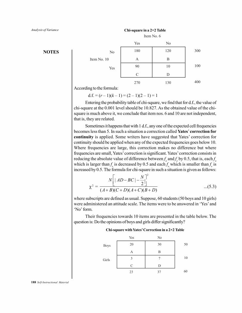
188 Self-Instructional Material
Analysis of Variance
NOTES
Chi-square in a 2×2 Table
Yes
Item No. 6
No
180 120
A B
90 10
C D
270 130
No
Yes
Item No. 10
300
100
400According to the formula:
d.f. = (r – 1)(k – 1) = (2 – 1)(2 – 1) = 1Entering the probability table of chi-square, we find that for d.f., the value of
chi-square at the 0.001 level should be 10.827. As the obtained value of the chi-square is much above it, we conclude that item nos. 6 and 10 are not independent,that is, they are related.
Sometimes it happens that with 1 d.f., any one of the expected cell frequenciesbecomes less than 5. In such a situation a correction called Yates’ correction forcontinuity is applied. Some writers have suggested that Yates’ correction forcontinuity should be applied when any of the expected frequencies goes below 10.Where frequencies are large, this correction makes no difference but wherefrequencies are small, Yates’ correction is significant. Yates’ correction consists inreducing the absolute value of difference between fo and fe by 0.5, that is, each fowhich is larger than fe is decreased by 0.5 and each fo which is smaller than fe isincreased by 0.5. The formula for chi-square in such a situation is given as follows:
χ2 =
2
| |2
( )( )( )( )
NN AD BC
A B C D A C B D
− − + + + +
...(5.3)
where subscripts are defined as usual. Suppose, 60 students (50 boys and 10 girls)were administered an attitude scale. The items were to be answered in ‘Yes’ and‘No’ form.
Their frequencies towards 10 items are presented in the table below. Thequestion is: Do the opinions of boys and girls differ significantly?
Chi-square with Yates’ Correction in a 2×2 Table
Yes No
20 30
A B
3 7
C D
23 37
Boys
Girls
50
10
60

Analysis of Variance
NOTES
Self-Instructional Material 189
According to Equation (5.3):
χ2 =
260| (20)(7) (30)(3) |260
(50)(10)(23)(37)
− −
= 260 |140 90 | 30] 60 400 24000 0.056
425500 425500 425500− − ×
= = =
In the above example, the expected frequency (23×10/60) is less than 5.Hence, chi-square has been calculated by Equation (5.3). Entering the table for chi-square, we find that for d.f. = 1, the value of chi-square at the 0.05 level should be3.841. Since the obtained value is less than it (P >> 0.05), one concludes that theopinions of boys and girls do not differ significantly.
5.3.2 Mann-Whitney U Test
The Mann-Whitney U test is a non-parametric substitute for the parametric t test.This test was independently proposed by Mann and Whitney. The Mann-Whitney Utest is used when the researcher is interested in testing the significance of differencebetween two independently drawn samples or groups. For applications of the U testit is essential that the data be obtained on ordinal measurement, that is, they musthave been obtained in terms of rank. Where the data have been obtained in terms ofscores, for application of the Mann-Whitney U test, it is essential that those scoresbe converted into rank without much loss of information. It is not necessary for theapplication of the Mann-Whitney U test that both groups must have unequal size.However, this test can also be applied to groups having equal size.
Here the calculation of the Mann-Whitney U test, which are concerned withlarger sample size of more than 20 cases is given:
U = 1 11 2 1
( 1)2
N NN N R++ − Σ ...(5.4)
U = 2 21 2 2
( 1)2
N NN N R++ − Σ ...(5.5)
Table 5.4 presents the scores of two groups on the Lie scale. Group I has10 subjects and Group II has 21 subjects. The first step is to rank all the scores inone combined distribution in an increasing order of size. The lowest score (takingboth sets of scores together) is 7 (second column) and hence, it is given a rank of1. The nest score is 8, which is again in the second column and it has been givena rank of 2. The third score from below is 10 (in the first column), which has beengiven a rank of 3. In this way, ranking is continued until all scores receive ranks.Subsequently, the two columns of ranks are summed. At this point, a check onarithmetical calculation is imposed. The check is that the sums of these two columnsmust be equal to N (N + 1)/2.

190 Self-Instructional Material
Analysis of Variance
NOTES
Check: 1 2( )( 1) (31)(32)88.5 407.5 496; 496
2 2N NR R +
Σ + Σ = = + = =
Hence, we can proceed:(by Equation 5.4)
U = 1 11 2 1
( 1)2
N NN N R++ − Σ =
(10)(10 1)(10)(21) 88.5 176.52
++ − =
(by Equation 5.5)
U = 2 21 2 2
( 1)2
N NN N R++ − Σ =
(21)(21 1)(10)(21) 407.5 33.52
++ − =
Table 5.4 Calculation of the Mann-Whitney U Test from Larger Sample Sizes
Gr. I Gr. II R1 R2(N1 = 10) (N2 = 21)
18 32 7 1314 40 15 1830 31 11 1210 39 3 16.539 15 16.5 626 8 9 227 47 10 1919 33 8 1435 52 15 2211 48 4 20
7 150 2161 2758 2453 2359 2560 2665 3063 2867 3164 29
ΣR1 = 88.5 ΣR2 = 407.5
It is the lower value of U test that one wants. For testing the significance ofthe obtained U, its values are converted into Z score as shown:
Z =
1 2
1 2 1 2
2( )( )( 1)
12
N NU
N N N N
−
+ +...(5.6)

Analysis of Variance
NOTES
Self-Instructional Material 191
=
(10)(21)176.5 71.52 3.0223.664(10)(21)(10 21 1)
12
−= =
+ +
A Z score from +1.96 to +2.58 is taken to be significant at the 0.05 level ofsignificance and if the Z score is greater than even +2.58, one takes it to be significantat the 0.01 level. Since the obtained Z is 3.02, on can take the value of the Mann-Whitney U to be a significant one. Rejecting the null hypothesis, one can concludethat the two groups differ significantly on the measures of the Lie scale.
5.3.3 Rank-difference MethodsThe methods of correlation based upon rank differences are very common amongbehavioural scientists. These are two most common methods which are based uponthe differences in ranks assigned on the X and Y variables. One is the Spearmanrank-difference method and the other is the Kendall rank-difference method. TheSpearman rank-difference method symbolized by ρ (read as rho) is a very popularmethod of computing the correlation coefficient between two sets of ranks or betweentwo sets of scores converted into ranks. The method has been named after Spearmanwho discovered it. This method is applicable when the number of pairs of scores orranks is preferably small, that is, 30 or below.The equation is:
ρ = 2
2
61
( 1)D
N N−
−∑
...(5.7)
where ρ = Spearman’s rank-difference correlation coefficient; D = differencebetween rank1 and rank2; and N = Number of pairs of ranks or scores.
To illustrate the calculation of ρ consider the data given in Table 5.5 thatfollows, which show the scores of 12 students on the intelligence test (X) as well ason the educational test (Y). The first step is to rank both sets of scores separatelygiving the highest score a rank of 1, the next highest score a rank of 2, and so on.Then, keeping the algebraic signs in view, the difference between two sets of ranksis computed. This is noted under column D. Subsequently, each difference is squaredand noted under column D2. Substituting the values in the equation, we get a ρ of –0.185. Following the table of Guilford (1956: Table L, p. 549), we can test thesignificance of the obtained ρ. Since the obtained value of ρ is less than the valuegiven at the 0.05 level (ρ > 0.05) for N = 12, one can accept the null hypothesis andcan conclude that X and Y are independent and whatever correlation has been foundis due to the chance factor.

192 Self-Instructional Material
Analysis of Variance
NOTES
Table 5.5 Illustration of the Spearman Rank-Difference Correlation
X Y Rank1 Rank2 D (R1 – R2) D2
47 68 8.5 1 +7.5 56.2550 60 5.5 2.5 +3 9.0070 54 2 7 –5 25.0072 53 1 8 –7 49.0046 60 10 2.5 –7.5 56.2550 55 5.5 6 –0.5 0.2542 48 11 9 +2 4.0058 30 3 12 –9 81.0055 45 4 10 –6 36.0036 43 12 11 +1 1.0049 59 7 4 +3 9.0047 56 8.5 5 +3.5 12.25
ΣD = 0.0 ΣD2 = 339.00
ρ = 6(339) 20341 1 1 1.185 0.18512(122 1) 1716
− = − = − = −−
Another method of computing the rank-difference correlation has beendeveloped by Kendall. The method is known as Kendall’s τ for which the formulais as follows.
τ = (1/ 2) ( 1)S
N N − ...(5.8)
where τ = Kendall’s τ, S = actual total; and N = number of objects or scores whichhave been ranked.
Suppose 12 students have been administered two tests and their scores arepresented in the following table.
Scores of 12 students on X and Y Test
A B C D E F G H I J K L X 20 26 17 16 15 23 22 24 19 28 30 10 Y 70 80 40 45 38 49 77 76 72 47 36 35
The first step is to rank both sets of scores giving the highest score a rank of1, the next higher a rank of 2, and so on. The following table presents the ranksbased upon two sets of the scores given in that table above. Subsequently, the ranksof the X test are rearranged in a way that they appear in a natural order like 1, 2, 3.
Ranks based upon two sets of scores given in the above table
A B C D E F G H I J K L X 7 3 9 10 11 5 6 4 8 2 1 12 Y 5 1 9 8 10 6 2 3 4 7 11 12

Analysis of Variance
NOTES
Self-Instructional Material 193
Accordingly, ranks on the Y test are adjusted. The following table presentsthe ranks in a rearranged order. Subsequently, the value of S is computed. For this,we start with the rank on the Y test from the left side.
Rearranged order of ranks
A B C D E F G H I J K L X 1 2 3 4 5 6 7 8 9 10 11 12 Y 11 7 1 3 6 2 5 4 9 8 10 12
The first rank on the left side is 11. Count the number of ranks which areabove 11 and the number of ranks which are below 11, separately. Only one rank(that is, 12) falling at the right of the first rank on the Y test is above 11 and theremaining 10 ranks fall below it. Hence, its contribution to S would be equal to1 – 10. Likewise, the second rank on the Y test is 7. The four ranks falling right of 7,are above 7 and 6 ranks are below it. Hence, its contribution to S would be 4 – 6.
Identical procedures are repeated for other ranks on the Y test. Thus:S = (1 – 10) + (4 – 6 ) + (7 – 1) + (4 – 3 ) + (6 – 0) + (4 – 1) + (4 – 0) +
(2 – 1) + (2 – 0) + (1 – 0) = (-9) + (-2) + (9) + (6) + (1) + (6) + (3) + (4) + (1) + (2)+ (1) = 33 – 11 = 22.Substituting this in the formula given in Equation (5.8):
τ = 22 22 0.3331 1 66( 1) 12(12 1)
2 2
S
N N= = =
− −
The significance of τ is tested by converting it into a Z score, the formula forwhich is as follows:
Z = 2(2 5)9 ( 1)
NN N
τ+−
...(5.9)
Hence
Z = 0.33 0.33 0.3 1.4938
0.22092[(2)(12) 5)] 0.04889(12)(12 1)
= = =+−
Since the obtained Z score is less than 1.96, one can say that this is notsignificant even at the 0.05 level. Accepting the null hypothesis, one can say that thegiven set of scores is not correlated. According to Siegel (1956), τ has one advantageover ρ, and that is that the former can be generalized to partial correlation. If both τand ρ are computed from the same data, the answer will not be the same and hence,numerically, they are not equal.

194 Self-Instructional Material
Analysis of Variance
NOTES
5.3.4 Coefficient Concordance, W
The coefficient of concordance symbolized by the letter W has been developed byKendall and is a measure of correlation between more than two sets of ranks. Thus,W is a measure of correlation between more than two sets of rankings of events,objects and individuals. When the investigator is interested in knowing the inter-testreliability, W is chosen as the most appropriate statistic. One characteristic of Wwhich distinguishes it from other methods of correlation is that it is either zero orpositive. It cannot be negative. W can be computed with the help of the formulagiven below:
W = 2 31 ( )
12
S
K N N−...(5.10)
where W = coefficient of concordance; S = sum of squares of deviations from themean of Rj; K = number of judges or sets of rankings; and N = number of objects orindividuals which have been ranked. Suppose four teachers (A, B, C and D) ranked8 students on the basis of performance shown in the classroom. The ranks given bythe four teachers are presented in the following table. The details of the calculationshave also been shown.
Ranks given by four teachers to eight students on thebasis of classroom performance
Students Teachers (i) (ii) (iii) (iv) (v) (vi) (vii) (viii)
A 3 4 7 5 8 6 2 1 B 2 3 6 4 8 7 1 5 C 1 3 5 6 8 7 2 4 D 3 4 2 5 7 6 1 8 Rj 9 14 20 20 31 26 6 18
Mean of Rj = 9 14 20 20 31 26 6 18 144 18
8 8+ + + + + + +
= =
S = (9 – 18)2 + (14 – 18)2 + (120 – 18)2 + (20 – 18)2 + (31 – 18)2
+ (26 – 18)2 + (6 – 18)2 + (18 – 18)2
= (– 9)2 + (– 4)2 + (2)2 + (2)2 + (13)2 + (8)2 + (–12)2 + (0)2 = 482Now substituting in Equation (8.21):
W = 2 3
482 482 0.717 0.721 672(4) (8 8)12
= = =−
when N > 7, the significance of W is tested by converting its value into χ2 with thehelp of the following equation: χ2 = K (N – 1) W. Thus, X2 = 4 (8 – 1) × 0.72= 20.16 and d.f. in this situation is always equal to N – 1. Hence d.f. = 8 – 1 = 7.

Analysis of Variance
NOTES
Self-Instructional Material 195
From the probability table for chi-square we find that the value of chi-square ford.f. = 7 at 0.05 level of significance should be 18.475. Since the obtained value ofthe chi-square exceeds this required value, one can take this value of W as a significantone. Thus rejecting the null hypothesis, one can say that there is an overall significantrelationship in ranking done by the four teachers.
5.3.5 Median Test
The median test is used to see if two groups (not necessarily of same size) comefrom the same population or from populations having the same median. In the mediantest, the null hypothesis is that there is no difference between the two sets of scoresbecause they have been taken from the same population. If the null hypothesis istrue, half of the scores in both the groups should lie above the median and theremaining half of the scores should lie below the median. The following table presentsthe scores of two groups of students in an arithmetic test. The first step in thecomputation of a median test is to compute a common median for both distributionstaken together.
Scores of 30 Students on an Arithmetic Test
Gr. B (N = 16) 16, 17, 8, 12, 14, 9, 7, 5, 20, 22, 4, 26, 27, 5, 10, 19
Gr. B (N = 14) 28, 30, 33, 40, 45, 47, 40, 38, 42, 50, 20, 18, 18, 19
For computing the common median, both the distributions are pulled togetheras shown in the following table:
Scores f
49–53
44–48
39–43
34–38
29–23
24–28
19–23
14–18
9–13
4–8
1
2
3
1
2
3
5
5
3
5
= 30N
( /2 – )Median = 1+
(30 / 2 13)518.55
20.5
m
N F if
−= +
=
Subsequently, a 2×2 contingency table is built as follows:Now, the chi-square test can be applied. For computing chi-square from a
2×2 table, we may follow the equation for Chi-square (χ2). Yates’ correction is notneeded here because none of the cells contain an expected frequency less than 5.

196 Self-Instructional Material
Analysis of Variance
NOTES
AboveMdn
Not aboveMdn
A B3 13
C D10 4
13 17
Gr. A 16
14
30
Now substituting the values in Equation (5.2) we get:
χ2 = 230[| 3(4) (13)(10) |]
(16)(14)(13)(17)−
= 230[|12 130 |] 417720 8.438 8.44
49504 49504−
= = =
df = (r – 1)(c – 1) = (2 – 1)(2 – 1) = 1
From the probability table for chi-square, we find that for d.f. = 1 the chi-square value at the 0.01 level should be 6.635. Since the obtained value of the chi-square exceeds this value (p < 0.01), we can reject the null hypothesis and concludethat the two samples have not been drawn from the same population or frompopulations having equal medians.
5.3.6 Kruskal-Wallis H Test
The primary difference between the F test and the Kruskal-Wallis H test on the onehand and the Friedman test on the other hand is that the F test is a parametricanalysis of variance, whereas the H test and Friedman test are the non-parametricanalysis. The H test is a one-way non-parametric analysis of variance and theFriedman test is a two-way non-parametric analysis of variance.
Table 5.6 H Test from Scores Obtained by Three Groups on Lie Scale
Gr.A (N = 6) Gr. B (N = 8) Gr. C (N = 10) 15 (14) 17 (15) 20 (17) 10 (9) 9 (8) 25 (19) 8 (3) 8 (6) 13 (12) 5 (4) 14 (13) 11 (10) 6 2) 2 (1) 26 (20) 4 8 (6) 24 (18) 12 (11) 36 (24) 18 (16) 30 (23) 29 (22) 27 (21)
Rj = 38 Rj = 76 Rj = 186
The H test is used when the investigator is interested in knowing whether ornot groups of the independent samples have been drawn from the same population.

Analysis of Variance
NOTES
Self-Instructional Material 197
If the obtained data does not fulfill the two basic parametric assumptions, namely,the assumptions of normality and the assumption of homogeneity of variances, theH test is the most appropriate statistic. The equation for the H test is as given asfollows:
H = 212 3( 1)
( 1)j
j
RN
N N N
− + +
∑ ...(5.11)
Where N = number in all samples combined; Rj = sum of ranks in j sample; and Nj =number in j sample.
Data to illustrate the calculation of the H test have been given in Table 8.6.Three groups of students were administered a Lie Scale and their scores are presentedin Table 5.6. The first step is to combine all the scores from all of the groups andrank them with the lowest score receiving a rank of 1 and the largest score by rankN. Ties are treated in usual fashion in ranking subsequently, the sum of ranks in eachgroup or column is found and the H test determines where these sums of ranks areso disparate that the three groups cannot be regarded as being drawn from the samepopulation. The ranks assigned to each score earned by the member of the groupare given in brackets. Now, substituting the value in the equation given in 5.11. weget:
H = 2 2 212 (38) (76) (186) 3(24 1)
(24)(25) 6 8 10
+ + − + ∑
= 53067.192 75 88.445 75 13.445 13.44
600− = − = =
When each sample has six or more than six cases, the H test is interpretedas chi-square. In such a situation, d.f. = number of groups or samples minus one.So, here d.f. = 2. Entering the probability table for chi-square, we find that ford.f. = 2, the value of chi-square at the level of significance should be 9.210. Sincethe obtained value of H test exceeds this required value, it can be said that theH value is significant. Rejecting the null hypothesis, one concludes that the samplesare independent and that they have not been drawn from the same population.
5.3.7 Friedman Test
The Friedman test is a two-way non-parametric analysis of variance. When thegroups are matched, doubts exist about the two basic parametric assumptions, namely,the assumption of normality and the assumption of homogeneity of variances, theinvestigator resorts to the Friedman test for testing whether or not the samples havebeen drawn from the same population. To illustrate this, the calculations of theFriedman test have been presented in Table 5.7. The following equation calculatesthe Friedman test is as follows:
2rX =
212 ( ) 3 ( 1)( 1) jR N K
NK K− +
+ ...(5.12)

198 Self-Instructional Material
Analysis of Variance
NOTES
where 2rX = Friedman test; N = number of rows; K = number of columns; and Rj =
separate sums of ranks of each column.
Table 5.7 Friedman Test of Two-way ANOVA from Scoresof Three Groups on Recall Test
I II III IV V Gr. A 12(4) 8(2) 4(1) 10(3) 16(5) Gr. B 10(3) 7(2) 6(1) 11(4) 17(5) Gr. C 7(2) 83) 4(1) 12(5) 10(4)
Rj 9 7 3 12 14
The first step in calculation of the Friedman test is to rank each score in eachrow separately giving the lowest score in each row a rank of 1 and the next lowestscore in each row a rank of 2, and so on. The ranking can also be done in reversedorder, that is, giving the highest score in each row a rank of 1, the next highest scorein each row a rank of 2, and so on. Rank assigned to each score in each row is givenin parentheses. The Friedman test is applied to determine whether or not the ranktotals symbolized by Rj differs significantly. Now, substituting the values in theequation of chi-square, we get
2rX = 2 2 2 212 (9) (7) (3) (14) 3(3)(5 1)
(3)(5)(5 1) + + + − + +
= 63.866 – 54 = 9.87
When the number or rows (N) and the number of columns (K) are toosmall, the significance of the Friedman test can be ascertained with the help ofspecial tables (Siegel, 1956). For example, when K = 4, N = 2 to 4 or when K= 3, N = 2 to 9, the significance of the Friedman test can be done through thesespecial tables. But when the number of rows and the number of columns aregreater than those said above, the Friedman test is interpreted as the chi-squaretest. In the present example, the significance of the Friedman test would beinterpreted in terms of chi-square. The d.f. is always equal to K – 1 for chi-square applied as a test of significance of the Friedman test. Hence d.f. in thepresent example would be K – 1 = 5 – 1 = 4. Entering the table for d.f. 4, wefind that the chi-square should be 9.488 at the 0.05 level of significance. Sincethe obtained value of the Friedman test exceeds this value (p < 0.05), one rejectsthe null hypothesis and conclude that three matched groups differ significantly.
CHECK YOUR PROGRESS
3. Name any three important non-parametric tests.4. When is the Mann-Whitney U test used?5. What is the Friedman Test?

Analysis of Variance
NOTES
Self-Instructional Material 199
5.4 SUMMARY
• ANalysis Of VAriance or ANOVA is one of the most powerful techniques instatistical analysis and was developed by R.A. Fisher. It is also called the F-Test. There are two types of classifications involved in the analysis of variance.The one-way analysis of variance refers to the situations when only one factor variable is considered. In the second type of classification, the responsevariable of interest may be affected by more than one factor.
• The basic principle of ANOVA is to test for differences among the means ofthe populations by examining the amount of variation within each of thesesamples, relative to the amount of variation between the samples.
• In case of a two-way design with repeated measurements for all thecategories, we can obtain a separate independent measure of inherent orsmallest variations. For this measure, we can calculate the sum of squaresand degrees of freedom in the same way as we have worked out the sum ofsquares for variance within samples.
• In the case of one-way ANOVA, SS total, SS between columns and SSbetween rows can also be worked out as stated above. We then find left-over sums of squares and left-over degrees of freedom which are used forwhat is known as ‘interaction variation’. Interaction is the measure of inter-relationship among the two different classifications. After making all thesecomputations, ANOVA table can be set up for drawing inferences.
• The important non-parametric statistics are as follows: (a) Chi-square (χ2)Test (b) Mann-Whitney U test (c) Rank-difference methods (both ρ and T)(d) Coefficient of concordance (W) (e) Median Test (f) Kruskal-WallisH Test (g) Friedman test.
• The chi-square is one of the most important non-parametric statistics, whichis used for several purposes. For this reason, Guilford (1956) has called it thegeneral-purpose statistic. It is a non-parametric statistic because it involvesno assumption regarding the normalcy of distribution or homogeneity of thevariances. The chi-square test is used when the data are expressed in termsof frequencies of proportions or percentages.
• The Mann-Whitney U test is a non-parametric substitute for the parametric ttest. This test was independently proposed by Mann and Whitney. The Mann-Whitney U test is used when the researcher is interested in testing thesignificance of difference between two independently drawn samples orgroups.
• The methods of correlation based upon rank differences are very commonamong behavioural scientists. These are two most common methods whichare based upon the differences in ranks assigned on the X and Y variables.One is the Spearman rank-difference method and the other is the Kendallrank-difference method.

200 Self-Instructional Material
Analysis of Variance
NOTES
• The coefficient of concordance symbolized by the letter W has been developedby Kendall and is a measure of correlation between more than two sets ofranks. Thus, W is a measure of correlation between more than two sets ofrankings of events, objects and individuals. When the investigator is interestedin knowing the inter-test reliability, W is chosen as the most appropriatestatistic.
• The median test is used to see if two groups (not necessarily of same size)come from the same population or from populations having the same median.In the median test, the null hypothesis is that there is no difference betweenthe two sets of scores because they have been taken from the samepopulation.
• The primary difference between the F test and the Kruskal-Wallis H test onthe one hand and the Friedman test on the other hand is that the F test is aparametric analysis of variance, whereas the H test and Friedman test arethe non-parametric analysis. The H test is a one-way non-parametric analysisof variance and the Friedman test is a two-way non-parametric analysis ofvariance.
• The Friedman test is a two-way non-parametric analysis of variance. Whenthe groups are matched, doubts exist about the two basic parametricassumptions, namely, the assumption of normality and the assumption ofhomogeneity of variances, the investigator resorts to the Friedman test fortesting whether or not the samples have been drawn from the samepopulation.
5.5 KEY TERMS
• ANOVA: Its full form is analysis of variance and it tests for differencesamong the means of the populations by examining the amount of variationwithin each of these samples, relative to the amount of variation between thesamples.
• One-way ANOVA: It is a technique used to compare means of two or moresamples using the F distribution and can be used only for numerical data.
• Chi-square (χ2) Test: It is a non-parametric statistic because it involves noassumption regarding the normalcy of distribution or homogeneity of thevariances.
• Mann-Whitney U Test: It is used when the researcher is interested intesting the significance of difference between two independently drawnsamples or groups.

Analysis of Variance
NOTES
Self-Instructional Material 201
5.6 ANSWERS TO ‘CHECK YOUR PROGRESS’
1. The basic principle of ANOVA is to test for differences among the means ofthe populations by examining the amount of variation within each of thesesamples, relative to the amount of variation between the samples.
2. Two basic assumptions underlying the technique of analysing variance are asfollows:• The population distribution should be normal. This assumption is, however,
not so important. The study of Norton (Guilford, 1965) also points out that‘F’ is rather insensitive to variations in the shape of population distribution.
• The sub-groups under investigation must have the same variability. Inother words, there should be homogeneity of variance.
3. The three important non-parametric tests are as follows:• Chi-square (χ2) Test• Mann-Whitney U test• Rank-difference methods (both ρ and T)
4. The Mann-Whitney U test is used when the researcher is interested in testingthe significance of the difference between two independently drawn samplesor groups.
5. The Friedman test is a two-way non-parametric analysis of variance. Whenthe groups are matched, doubts exist about the two basic parametricassumptions, namely, the assumption of normality and the assumption ofhomogeneity of variances, the investigator resorts to the Friedman test fortesting whether or not the samples have been drawn from the same population.
5.7 QUESTIONS AND EXERCISES
Short-Answer Questions1. What are the two types of classification involved in the analysis of variance?2. Why is the two-way ANOVA technique used?3. Discuss one-way ANOVA in detail with examples.4. State the uses of Chi-square (χ2) Test.5. List the importance of rank-difference methods.
Long-Answer Questions1. Explain the test to determine the differences within the factor under the one-
way ANOVA.
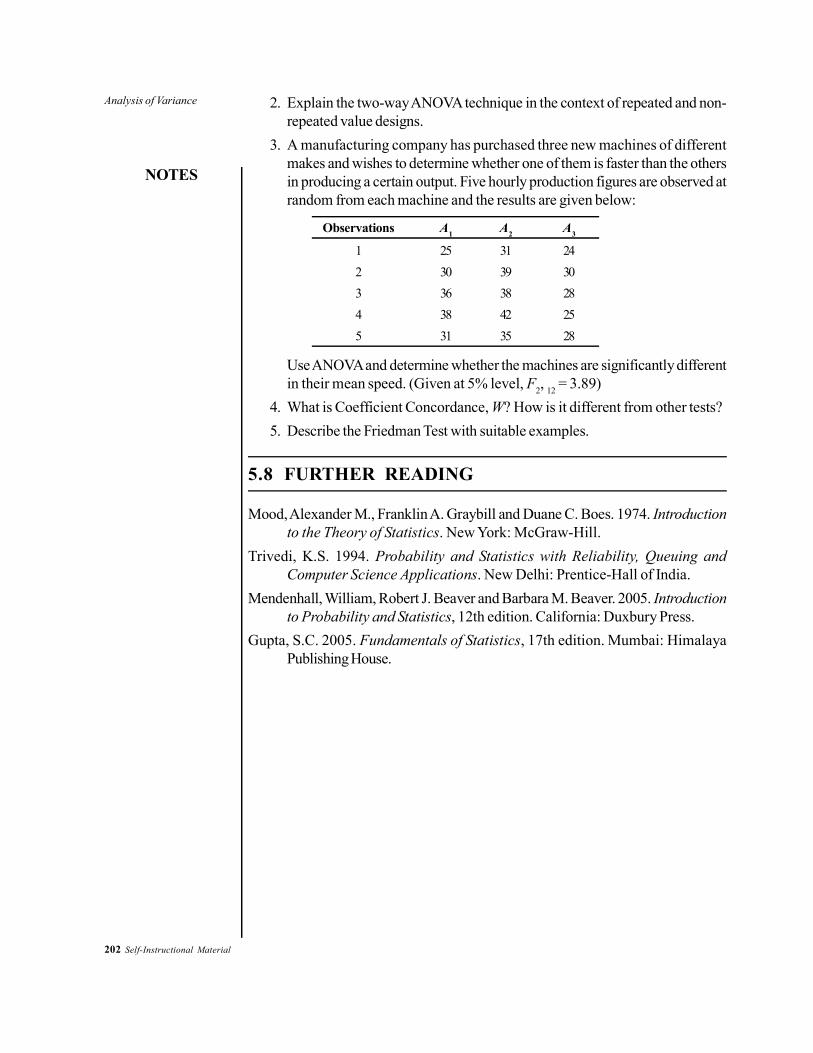
202 Self-Instructional Material
Analysis of Variance
NOTES
2. Explain the two-way ANOVA technique in the context of repeated and non-repeated value designs.
3. A manufacturing company has purchased three new machines of differentmakes and wishes to determine whether one of them is faster than the othersin producing a certain output. Five hourly production figures are observed atrandom from each machine and the results are given below:
Observations A1 A2 A3
1 25 31 242 30 39 303 36 38 284 38 42 255 31 35 28
Use ANOVA and determine whether the machines are significantly differentin their mean speed. (Given at 5% level, F2, 12 = 3.89)
4. What is Coefficient Concordance, W? How is it different from other tests?5. Describe the Friedman Test with suitable examples.
5.8 FURTHER READING
Mood, Alexander M., Franklin A. Graybill and Duane C. Boes. 1974. Introductionto the Theory of Statistics. New York: McGraw-Hill.
Trivedi, K.S. 1994. Probability and Statistics with Reliability, Queuing andComputer Science Applications. New Delhi: Prentice-Hall of India.
Mendenhall, William, Robert J. Beaver and Barbara M. Beaver. 2005. Introductionto Probability and Statistics, 12th edition. California: Duxbury Press.
Gupta, S.C. 2005. Fundamentals of Statistics, 17th edition. Mumbai: HimalayaPublishing House.