SIMPLE LINEAR REGRESSION MODEL AND MATLAB CODE

COMSATS Institute Of IT Attock Campus

Linear regression model

SIMPLE LINEAR REGRESSION MODEL AND MATLAB CODE

--Manuscript draft--

Full Title Simple linear regression model and Matlab code

Abstract The relationship among variable may or may not be governed by an exact

physical law. For convenience, let us consider a set of npairs of

observation(Xi,Yi). If the relation between the variables is exactly linear, then the

mathematical equation describing the linear relation is generally written as

(Yi=a+bXi) where a is the value of Y when X=0 and is called y intercept and b

indicate the change in Y for one unit change in X and is called the slop.

Substituting a value of X in the equation, can completely determine the a unique

value of y. the linear relation in such case is called a deterministic model. When

the equation involves an error in such case the equation is called the non-

deterministic or probabilistic model. The term regression investigates the

dependence of one variable on other. When we study the dependence of a

variable on a single independent variable then it is called simple or linear

regression.



Zahoor ahmad1,Faseehullah

2,Waqas latif

2,M.annas

2,Kamran ali

2

Comsats Institute Of Information Technology,Islamabad,Pakistan

1.1 Abstract:

The relationship among variable may or may not be governed by an exact physical law. For

convenience, let us consider a set of npairs of observation(Xi,Yi). If the relation between the

variables is exactly linear, then the mathematical equation describing the linear relation is

generally written as (Yi=a+bXi) where a is the value of Y when X=0 and is called y intercept

and b indicate the change in Y for one unit change in X and is called the slop. Substituting a

value of X in the equation, can completely determine the a unique value of y. the linear

relation is such case is called a deterministic model. When the equation involves an error in

such case the equation is called the non-deterministic or probabilistic model. The term

regression investigates the dependence of one variable on other. When we study the

dependence of a variable on a single independent variable then it is called simple or linear

regression.

1.2 introduction :

History: the term regression was introduce by the English biometrician, Sir Francis

Galton (1872-1911) to describe a phenomenon which he observed in analyzing the

heights of children and their parents. He found that tall parents have tall children and

short parents have short children, the average height of the children tends to step back

or to regress toward the average height of all men. This tendency toward the average

height of all men was called a regression by Galton.

i) Introduction to linear regression: today the word regression is used in a quite

different sense. It investigates the dependence of one variable, conventionally called

the dependent variable, on one or more other variables, called independent variables,

and provides an equation to be used for estimating or predicting the average value of

the dependent variable from known values of the independent variable. The

dependent variable is assumed to be a random variable whereas the independent

variable are assume to have a fixed value, i.e. they are chosen non-randomly. The

relation between the expected value of dependent variable and the independent

variable is called a regression model. When we study the dependence of a variable on

a single independent variable, it is called a simple or linear or two-variable

regression. When the dependence of a variable on two or more the two independent

variable is studied, it is called multiple linear regression. Furthermore, when the

dependence is represented by a straight line equation, the regression is said to be

linear, otherwise it is said to be curvilinear.



1.3 simple linear regression; we assume that the linear relationship between the dependent

variable Yi and the value Xi of the regression X is

Yi = α + βxi + £i

Where the Xi’s are the fixed or predetermined values,

The Yi’s are observations randomly drawn from a population,

The £i’s are error components or random deviations,

αand β are population parameters, α is the intercept and the slop β is called the regression

coefficient, which may be positive or negative depending upon the direction of the

relationship between X and Y.

Furthermore, we assume that

i) E(£i) = 0, i.e the expected value of error is zero.it means that this is a straight line

ii) varE(£i) = E(£i)2 for all i, i.e the variance of error term is constant. It means that the

distribution of the error has the same variance for all values of X.

iii) E(£I,£j) = 0 for all i ≠ j, i.e error term are independent of each other.

iv) E(X,£i) = 0 ,i.e X and £are also independent of each other.

v) £i’s are normally distributed with a mean of zero and constant variance ∂2

.this

implies that Y values are normally distributed. The distribution of Y and £ are

identical except that they have different means. This assumption is required for

estimation and tasting of hypothesis in all linear regression.

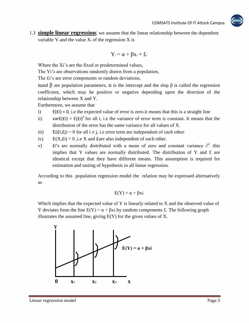
According to this population regression model the relation may be expressed alternatively

as

E(Y) = α + βxi

Which implies that the expected value of Y is linearly related to X and the observed value of

Y deviates from the line E(Y) = α + βxi by random components £. The following graph

illustrates the assumed line, giving E(Y) for the given values of X.

Y

E(Y) = α + βxi

0 x1 x2 x3 x



but in practical, we have a sample from some population, therefor we desire to estimate the

population regression line from the simple data. Then the basic relation in term of sample data

may be written as

Yi = a + bxi + ei

Where a, b and eiare the estimate of α , β and £.

1.3.1 The Principle of least squares :The principle of least squares (LS) consist of

determining the values of unknown parameters that will minimize the sum of errors.

The parameter values thus determine, will give the least sum of the squares of errors and

are known as leastsquare estimates.

1.3.1.aHistory of the principle least square : the method of least square that gets its

name from the minimization of sum of square deviation is attributed to Karl F. Gauss(1777-

1855). Some people believe that the method was discovered at the same time by Adrian M.

Legendre(1752-1833). Pierre S, Laplace(1749-1827) and others.



1.4.1The goal of linear and nonlinear regression :

A line is described by a simple equation that calculates Y from X, slope and intercept. The

purpose of linear regressionis to find values for the slope and intercept that define the line

that comes closest to the data.

Nonlinear regressionis more general than linear regression and can fit data to any equation

that defines Y as a function of X and one or more parameters. It finds the values of those

parameters that generate the curve that comes closest to the data.

1.5.1Common life example of linear regression :

Statistical analysis is the basis of modern life. Statistical analysis has allowed us to create

powerful medicines that cure disease. They have allowed us to create cars that are safe,

products that meet our needs and corporations that offer services that people only dreamed

about a century ago. Almost every organization today uses statistical analysis to ensure

profitability. And yet most people feel that statistical analysis is intimidating. This article will

show you how simple and practical statistics can be by illustrating a simple linear regression

example. will teach you how to use descriptive statistical analysis techniques so that you can

summarize and analyze your own data.

Simple linear regression is a technique that displays the relationship between variable “y”

based on the values of variable “x”. In simple terms we use linear regression relationships all

the time in our own lives. We know as the temperature drops people put on more jackets to

keep warm or as the gas price increases more people drive less to save money. In fact,

economists rely on these relationships to manage the economy by increasing bank rates to

discourage lending.



1.6.1 Matlab code for linear regression :

n=input('Input number of data size (n):'); %ask for number of data points for i=1:n %loop for input the data points x(i)=input('Input x series one by one:'); %take the data for x y(i)=input('Input y series one by one:'); %take the data for y end scatter(x,y) %make a graph of data point for i=1:n %loop to calculate summition xy(i)=x(i)*y(i); %calculate the of x*y x2(i)=(x(i))^2; %calculate the of x square end sumx=sum(x); %calculate the sum of x sumy=sum(y); %calculate the sum of y sumxy=sum(xy); %calculate the sum of x*y sumx2=sum(x2); %calculate the sum of x square xm=sumx/n; %calculate the mean of x ym=sumy/n; %calculate the mean of y a1=(n*sumxy-sumx*sumy)/(n*sumx2-sumx*sumx) %calculate the b a0=ym-a1*xm %calculate the a for i=1:n %loop for 1=1 upto 9 st=(y(i)-ym)^2; %calculate the diffrence of y from mean sr=(y(i)-a1*x(i)-a0)^2; %calculat the least squear end sumst=sum(st); %sum of least square principle sumsr=sum(sr); %sum of least square principle syx=(sumsr/(n-2))^0.5; %calculate the value for least square r2=(sumst-sumsr)/sumst syx=(sumsr/(n-2))^0.5; r2=(sumst-sumsr)/sumst

output :



Terminologies :

Population : collection or set of all possible observations.



Sample : a subset of population.

Mean : the most familier average.

Variance : a set of observations is define as the mean of the squares of deviations of

all the observations from there mean.

Slop : rise over run.

Intercept :The x-intercepts are where the graph crosses the x-axis, and the y-

intercepts are where the graph crosses the y-axis.

Random variable : A random variable can take on a set of possible different values

(similarly to other mathematical variables).

Curvilinear : consisting of, bounded by, or characterized by a curved line.



[revised jan 2015]

SIMPLE LINEAR REGRESSION MODEL AND MATLAB CODE

Documents

Transcript of SIMPLE LINEAR REGRESSION MODEL AND MATLAB CODE