RESEARCH ARTICLE10.1002/2014WR016192

A new frequency domain analytical solution of a cascade ofdiffusive channels for flood routingLuigi Cimorelli1, Luca Cozzolino2, Renata Della Morte2, Domenico Pianese1, and Vijay P. Singh3

1Dipartimento di Ingegneria Civile, Edile e Ambientale, Universit�a degli Studi di Napoli Federico II, Napoli, Italy, 2CentroDirezionale di Napoli, Dipartimento di Ingegneria, Universit�a degli Studi di Napoli Parthenope, Napoli, Italy, 3Departmentof Biological and Agricultural Engineering and Zachry Department of Civil Engineering, Texas A&M University, CollegeStation, Texas, USA

Abstract Simplified flood propagation models are often employed in practical applications for hydraulicand hydrologic analyses. In this paper, we present a new numerical method for the solution of the LinearParabolic Approximation (LPA) of the De Saint Venant equations (DSVEs), accounting for the space variationof model parameters and the imposition of appropriate downstream boundary conditions. The new modelis based on the analytical solution of a cascade of linear diffusive channels in the Laplace Transform domain.The time domain solutions are obtained using a Fourier series approximation of the Laplace Inversion for-mula. The new Inverse Laplace Transform Diffusive Flood Routing model (ILTDFR) can be used as a buildingblock for the construction of real-time flood forecasting models or in optimization models, because it isunconditionally stable and allows fast and fairly precise computation.

1. Introduction

Flow routing models for flow propagation in channel networks are often obtained as simplified versions ofthe full De Saint Venant Equations [DSVEs). Nowadays, application of these simplified models to problems,such as real-time flood forecasting and operations management, is still common, despite the availability ofpowerful computing resources. This is justified by several reasons: (a) the lack of data about the channelgeometry and the associated floodplains introduces numerical errors that may counter the advantage ofusing the complete De Saint Venant Equations; (b) in many cases, the peculiar dynamics of the flow propa-gation make the solution of the simplified models sufficient for practical purposes; and (c) the accurate solu-tion of complete De Saint Venant models is very time consuming [Cozzolino et al., 2012]. On the other hand,simplified flood routing models may exhibit one or more of the following favorable characteristics: simpli-fied rating curves (nonlooped) can be employed, the knowledge of just one upstream boundary conditionis often required (discharge hydrograph or stage hydrograph), and the calibration of only few parameters isrequired; they are usually linear and errors in the input quantities are not amplified [Singh and Woolhiser,1976]; the simplified models allow fast computation and hence they are particularly suited for problems inwhich large and repetitive computations are required, such as the optimal design of hydraulic infrastruc-tures [Cimorelli et al., 2013a, 2014b; Palumbo et al., 2014; Cozzolino et al., 2015].

The well-known Parabolic Approximation (PA) model is derived from the DSVEs by neglecting the inertialterms, while the Kinematic Wave is obtained by neglecting also the pressure terms [Cunge et al., 1980].Despite the simplifications introduced, there are ranges of hydraulic conditions where satisfactory and accu-rate application of the PA model is found, as discussed in the scientific literature [Ponce and Simmons, 1977;Ponce et al., 1978; Tsai, 2003]. Weinmann and Laurenson [1979] showed that numerous approximate flowrouting models can be regarded as linearized versions of these simplified models. Among the linear flowrouting models, the Kalinin-Milyukov-Nash (KMN) reservoir cascade model [Nash, 1957; Kalinin and Milyukov,1957], the Muskingum-Cunge (MC) model [Cunge, 1969], and the Hayami [1951] transfer function (HTF)have been widely employed for discharge forecasting for large rivers [Singh, 1996]. The linear models areattractive for their simplicity and because model parameters are easily related to channel characteristicsand hydraulics conditions. However, it is widely recognized that the propagation of flood waves in channelsis a nonlinear process, and linear models can provide only a crude approximation of real flow propagationphenomena.

Key Points:� Frequency domain analytical solution� Nonuniform channel geometry and

downstream boundary condition areaccounted� Fast computation due to model

unconditional stability

Correspondence to:L. Cimorelli,luigi.cimorelli@unina.it

Citation:Cimorelli, L., L. Cozzolino,R. Della Morte, D. Pianese,and V. P. Singh (2015), A newfrequency domain analytical solutionof a cascade of diffusive channels forflood routing, Water Resour. Res., 51,doi:10.1002/2014WR016192.

Received 24 JUL 2014

Accepted 12 MAR 2015

Accepted article online 18 MAR 2015

VC 2015. American Geophysical Union.

All Rights Reserved.

CIMORELLI ET AL. FREQUENCY DOMAIN ANALYTICAL SOLUTION FOR FLOOD ROUTING 1

Water Resources Research

PUBLICATIONS

In order to account for nonlinearities, it can be assumed that the flood wave propagation responds linearlyto the input, but model parameters are recalculated as functions of local and instantaneous values of flowconditions during the marching-in-time of the algorithm. This idea has been incorporated into the develop-ment of a wide class of flood routing models known as multilinear models [Keefer and McQuivey, 1974;Ponce and Yevjevich, 1978; Becker and Kundzewicz, 1987; Perumal, 1992, 1994; Camacho and Lees, 1999; Szila-gyi, 2003, 2006; Perumal et al., 2007, 2009; Szilagyi and Laurinyecz, 2012], and has allowed the use of all thepreviously mentioned simplified linear models as submodels embedded into the multilinear methodology.This shows that the study of linear models in hydrology is still of great interest, because they can be used asbuilding blocks for the construction of nonlinear models.

The linear models derived from the PA model are particularly attractive, because they are able to take intoaccount not only the wave celerity but also its attenuation. The Hayami linear transfer function [Hayami,1951] is calculated assuming semiinfinite channel, and Todini and Bossi [1986] used the corresponding dis-crete impulse response to construct the Parabolic and Backwater (PAB) routing scheme. Later, Cimorelliet al. [2013b] extended the PAB in order to account for the hydraulic jumps and for pressurized flow inclosed conduits. Litrico et al. [2010] used cumulants of the Hayami transfer function to derive a nonlinearDelayed Differential Equation (DDE) through a family of linear DDEs. The main drawback of the cited modelsis that in the Hayami transfer function, downstream boundary conditions are not properly taken intoaccount. As highlighted by many authors [Chung et al., 1993; Singh, 1996; Tsai, 2005; Cozzolino et al., 2014a,2014b; Cimorelli et al., 2014a], the downstream boundary condition can significantly modify the flow dynam-ics. Chung et al. [1993] presented a Laplace-Domain analytical solution of the Linear Parabolic Approxima-tion (LPA) of DSVEs, accounting for the downstream boundary conditions in terms of discharge, while thecorresponding time-domain solution was determined through a Fourier series approximation of the Laplaceinversion formula [Crump, 1976]. An analytical solution in terms of discharge and flow depth, in both Lap-lace and time domains, was given in Cimorelli et al. [2014a], considering two different downstream bound-ary conditions and accounting for lateral inflow.

The cited linear flood routing models are derived under the hypothesis of prismatic channel and initial uni-form steady state. A step forward in simplified modeling of the linearized DSVEs was made by Litrico andFromion [2004], where the initial backwater curve was approximated by means of a cascade of prismaticpools with uniform initial conditions, and rational functions were used to fit the frequency response of thesystem. Of course, every new initial backwater curve requires a new fitting of the frequency response, andthis can be very time consuming in multilinear approaches. Munier et al. [2008] considered a cascade of twoprismatic channels with different flow and geometric characteristics, taking into account the downstreamboundary condition. The reference backwater curve was approximated by a piecewise constant curve, andthe transfer function of each channel was determined in the Laplace domain. The time-domain responsewas approximated by the solution of a simple ordinary differential equation, and parameters of the approxi-mated solutions were determined by the moment matching method. This model was used to route theinput hydrograph through an irrigation channel regulated by a gate or a weir at the downstream end, pro-viding satisfactory results with respect to the numerical solution of the full DSVEs. Nevertheless, in naturalrivers the geometry of cross sections can vary conspicuously along the river, and a cascade of two channelsmay not be sufficient for the approximation of the real flow behavior.

In this paper, we present a new spatially distributed flood routing model based on the Linearized ParabolicApproximation (LPA) of DSVEs, accounting for the space variation of model parameters and the down-stream boundary condition. The new model is based on the analytical solution of a cascade of linear diffu-sive channels in the Laplace Transform domain, while the time-domain solution is obtained via a FourierSeries approximation of the Laplace Transform Inversion Integral [Crump, 1976]. The new Inverse LaplaceTransform Diffusive Flood Routing (ILTDFR) model is suitable for real-time flood forecasting and optimiza-tion, because it allows fast computation and it is unconditionally stable. Moreover, it may serve as the linearsubmodel for a multilinear approach and hence it can be readily extended in order to account for nonlinear-ities in the flow propagation.

The present paper is organized as follows: first, the governing equations are briefly recalled; then the deriva-tion of the model and the discussion of the mathematical properties of the model are presented. The modelis evaluated making use of analytical and numerical reference solutions, and the results of laboratory experi-ments available in the literature. Finally, the paper is closed by conclusions in section 6.

Water Resources Research 10.1002/2014WR016192

CIMORELLI ET AL. FREQUENCY DOMAIN ANALYTICAL SOLUTION FOR FLOOD ROUTING 2

2. Basic Equations

2.1. Linear Parabolic Approximation of the DSVEsThe DSVEs are usually used to describe the one-dimensional flow in open channels:

B@h@t

1@Q@x

50

@Q@t

1@

@xQ2

A

� �1gA

@h@x

2S01J

� �50

:

8>>><>>>:

(1)

In equation (1), the symbols have the following meaning: x and t denote the space and time-independentvariables, respectively; h(x,t) is the water depth; Q(x,t) is the flow discharge; A(h,x) is the flow cross-sectionarea; S0 is the longitudinal bed slope; J(Q,h,x) is the friction slope; B(h,x) is the water surface width; and g isthe gravity acceleration.

In many practical applications, the inertial terms are small with respect to the gravity and pressure terms,and therefore they can be neglected, giving rise to the so-called Parabolic Approximation (PA) of the DSVEs:

B@h@t

1@Q@x

50

@h@x

2S01J50

:

8>><>>:

(2)

In Cimorelli et al. [2014a], the equations of the linear channel are obtained after the linearization of equation(2) around a steady uniform condition in a prismatic channel. Here a different approach is applied, and anonprismatic channel with nonuniform steady state condition is considered. The steady state condition ischaracterized by uniform discharge Q0, in order to satisfy the first of equation (2), while the variable flowdepth h 5 h0(x) and the uniform discharge Q0 satisfy together the second of equation (2) in the form

dh0

dx2S01J050; (3)

where J0(x) 5 J(Q0, h0(x), x). To linearize equation (2), the unknown variables Q(x,t) and h(x,t) are expandedaround the steady state flow conditions using the following form:

h x; tð Þ5h0 xð Þ1eh0 x; tð Þ1e2h00 x; tð Þ1:::; Q x; tð Þ5Q01eQ0

x; tð Þ1e2Q00

x; tð Þ1:::; (4)

Substituting equation (4) into equation (2), and neglecting the higher-order terms, the following Linear Par-abolic Approximation is obtained

B0@h0

@t1@Q

0

@x50

@h0

@x1

@J@h

� �0

h01@J@Q

� �0

Q050

:

8>>><>>>:

(5)

where B0(x)5B(h0(x), x), while @J=@hð Þ0 and @J=@Qð Þ0 are the derivatives @J=@h and @J=@Q calculated inQ0; h0 xð Þ; xð Þ, respectively.

The mathematical model obtained is linear, with coefficients B0, @J=@hð Þ0 and @J=@Qð Þ0, variable in space.Now, let Lc be the length of the channel. If a reference abscissa xr �[0, Lc] is assumed, together with refer-ence values hr and Qr of the flow variables, then it is possible to consider a first-order Taylor expansion ofthe coefficients contained in equation (5), and the following system is obtained:

Br@h0

@t1@Q

0

@x50

@h0

@x1

@J@h

� �rh01

@J@Q

� �rQ050

:

8>>><>>>:

(6)

where Br 5 B(hr, xr), while @J=@hð Þr and @J=@Qð Þr are the derivatives @J=@h and @J=@Q calculated inQr ; hr ; xrð Þ. Note that in equation (6), it must be Qr 5 Q0, while hr is the value of h at a reference point along

the channel that does not necessarily coincide with the abscissa xr.

Water Resources Research 10.1002/2014WR016192

CIMORELLI ET AL. FREQUENCY DOMAIN ANALYTICAL SOLUTION FOR FLOOD ROUTING 3

It is easy to see that equation (6) can be turned into advection-diffusion form as follows:

Br@h0

@t1@Q

0

@x50

@Q0

@t1Cr

@Q0

@x5Dr

@2Q0

@x2

;

8>>><>>>:

(7)

where

Cr521Br

@J@h

� �r

=@J@Q

� �r

; Dr51Br=

@J@Q

� �r

: (8)

Coefficient Cr is the celerity of the Linear Parabolic Approximation (LPA), while Dr is the diffusivity.

2.2. Laplace-Domain Approach for the LPAIn Cimorelli et al. [2014a], equation (7) is turned into dimensionless form using the transformations:

t�5t=s; x�5x=Lc; h�5h’=hr ; Q�5Q’=Qr ; (9)

where s5Lc=Cr is a characteristic time. The following system is obtained:

b@h�

@t�1@Q�

@x�50

@h�

@x�1r1Q�1r2h�50

;

8>><>>:

(10)

where

b5hr

QrBr Cr ; r15Lc

@J@Q

� �r

Qr

hr; r25

@J@h

� �rLc : (11)

Application of the Laplace transform to equation (10) with the initial conditions h*(x*,0) 5 0 and Q*(x*,0) 5 0 leads to

@Q_

@x�1b s� h

_

50

@h_

@x�1r1Q

_

1r2h_

50

;

8>>>><>>>>:

(12)

where s* is the Laplace counterpart of the dimensionless time variable t*, while Q and h are the Laplacetransforms of Q* and h*, respectively. In the following, the hat symbol will be used to indicate the Laplacetransform of a time-domain function y(t), i.e., y sð Þ5L y tð Þ½ � where L[•] is the Laplace transform operator. TheLaplace-domain general solution of equation (12) has the form

Q_

x�; s�ð Þ

h_

x�; s�ð Þ

24

355c x�; s�ð Þ

Q_

0; s�ð Þ

h_

0; s�ð Þ

24

35; (13)

and the expression of the state transition matrix c x�; s�ð Þ is given in Cimorelli et al. [2014a]. From a mathe-matical point of view, the components of the matrix c x�; s�ð Þ can be regarded as the Laplace-domainresponse at a given abscissa x* caused by the unit impulses of discharge and flow depth applied at theupstream end.

3. Laplace-Domain Solution for the Cascade of Diffusive Channels

Following Litrico and Fromion [2004] and Munier et al. [2008], the case of nonuniform reference flow condi-tions is approximated by means of a cascade of uniform channels characterized by different parameters. Inthis section, this approach is generalized, and the Laplace-domain solution of the cascade of diffusive chan-nels is presented and discussed.

Water Resources Research 10.1002/2014WR016192

CIMORELLI ET AL. FREQUENCY DOMAIN ANALYTICAL SOLUTION FOR FLOOD ROUTING 4

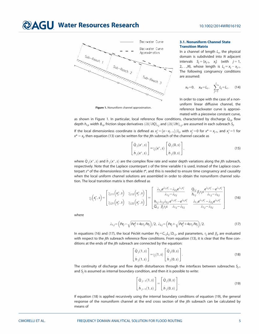
3.1. Nonuniform Channel StateTransition MatrixIn a channel of length Lc, the physicaldomain is subdivided into N adjacentintervals Sj 5 [xj-1, xj] (with j 5 1,2,. . .,N), whose length is Lj 5 xj 2 xj-1.The following congruency conditionsare assumed:

x050; xN5Lc;XL

j51

Lj5Lc: (14)

In order to cope with the case of a non-uniform linear diffusive channel, thereference backwater curve is approxi-mated with a piecewise constant curve,

as shown in Figure 1. In particular, local reference flow conditions, characterized by discharge Qr,j, flowdepth hr,j, width Br,j, friction slope derivatives @J=@Qð Þr;j and @J=@hð Þr;j , are assumed in each subreach Sj.

If the local dimensionless coordinate is defined as x�j 5 x2xj21� �

=Lj , with x�j 50 for x* 5 xj-1, and x�j 51 forx* 5 xj, then equation (13) can be written for the jth subreach of the channel cascade as

Q_

j x�; sð Þ

h_

j x�; sð Þ

24

355cj x�; sð Þ

Q_

j 0; sð Þ

h_

j 0; sð Þ

24

35; (15)

where Q_

j x�; sð Þ and h_

j x�; sð Þ are the complex flow rate and water depth variations along the jth subreach,respectively. Note that the Laplace counterpart s of the time variable t is used, instead of the Laplace coun-terpart s* of the dimensionless time variable t*, and this is needed to ensure time congruency and causalitywhen the local uniform channel solutions are assembled in order to obtain the nonuniform channel solu-tion. The local transition matrix is then defined as

cj x�j ; s� �

5

cj;11 x�j ; s� �

cj;12 x�j ; s� �

cj;21 x�j ; s� �

cj;22 x�j ; s� �

264

3755

k1;jek2;j x�j 2k2;je

k1;j x�j

k1;j2k2;j

Qr;j

hr;jbjsj s

ek2;j x�j 2ek1;j x�j

k1;j2k2;j

hr;j

Qr;j

k1;jk2;j

bjsjsek1;j x�j 2ek2;j x�j

k1;j2k2;j

k1;iek1;j x�j 2k2;j e

k2;j x�j

k1;j2k2;j

266664

377775 (16)

where

k1;j5 Pej2

ffiffiffiffiffiffiffiffiffiffiffiffiffiffiffiffiffiffiffiffiffiffiffiffiffiPe2

j 14ssj Pej

q� �=2; k2;j5 Pej1

ffiffiffiffiffiffiffiffiffiffiffiffiffiffiffiffiffiffiffiffiffiffiffiffiffiPe2

j 14ssj Pej

q� �=2: (17)

In equations (16) and (17), the local P�ecl�et number Pej5Cr;j Lj=Dr;j , and parameters, sj and bj, are evaluatedwith respect to the jth subreach reference flow conditions. From equation (13), it is clear that the flow con-ditions at the ends of the jth subreach are connected by the equation:

Q_

j 1; sð Þ

h_

j 1; sð Þ

24

355cj 1; sð Þ

Q_

j 0; sð Þ

h_

j 0; sð Þ

24

35: (18)

The continuity of discharge and flow depth disturbances through the interfaces between subreaches Sj-1

and Sj is assumed as internal boundary condition, and then it is possible to write:

Q_

j21 1; sð Þ

h_

j21 1; sð Þ

24

355

Q_

j 0; sð Þ

h_

j 0; sð Þ

24

35: (19)

If equation (18) is applied recursively using the internal boundary conditions of equation (19), the generalresponse of the nonuniform channel at the end cross section of the jth subreach can be calculated bymeans of

Figure 1. Nonuniform channel approximation.

Water Resources Research 10.1002/2014WR016192

CIMORELLI ET AL. FREQUENCY DOMAIN ANALYTICAL SOLUTION FOR FLOOD ROUTING 5

Q_

j 1; sð Þ

h_

j 1; sð Þ

24

355c jð Þ

c sð ÞQ_

1 0; sð Þ

h_

1 0; sð Þ

24

35; (20)

where the nonuniform state transition matrix is defined by

c jð Þc sð Þ5

Yj

r51

cj2r11 1; sð Þ: (21)

The product in equation (21) can be immediately calculated as c jð Þc sð Þ5cj 1; sð Þ c j21ð Þ

c sð Þ if c j21ð Þc sð Þ is known,

and the real and imaginary parts of its components are reported in Appendix A. It is easy to show that thedeterminant kc jð Þ

c sð Þk5c jð Þc;11 sð Þ c jð Þ

c;22 sð Þ2c jð Þc;12 sð Þ c jð Þ

c;21 sð Þ of c jð Þc sð Þ can be expressed as

kc jð Þc sð Þk5

Yj

r51

exp Per½ �: (22)

For j 5 N, equation (20) can be particularized as

Q_

N 1; sð Þ

h_

N 1; sð Þ

24

355c Nð Þ

c sð ÞQ_

1 0; sð Þ

h_

1 0; sð Þ

24

35; (23)

and matrix c Nð Þc sð Þ relates the discharge and flow depth disturbances at the downstream end of the nonuni-

form channel with the disturbances at the upstream end. Equation (23) can be rewritten as a system of twoequations as follows:

Q_

N 1; sð Þ5c Nð Þc;11 sð ÞQ

_

1 0; sð Þ1c Nð Þc;12 sð Þ h

_

1 0; sð Þ

h_

N 1; sð Þ5c Nð Þc;21 sð ÞQ

_

1 0; sð Þ1c Nð Þc;22 sð Þ h

_

1 0; sð Þ;

8><>: (24)

where c Nð Þc;lr sð Þ are the components of matrix c Nð Þ

c sð Þ. In the Laplace domain, coefficients c Nð Þc;11 sð Þ and c Nð Þ

c;12 sð Þrepresent the discharge response at the downstream end of the channel due to the discharge and flowdepth unit impulses, respectively, at the upstream end of the channel. Similarly, coefficients c Nð Þ

c;21 sð Þ andc Nð Þ

c;22 sð Þ represent the flow depth response at the downstream end of the channel due to the discharge andflow depth unit impulses, respectively, at the upstream end of the channel.

3.2. Downstream Boundary Condition and Impulse Response at the End of the ChannelThe use of equation (23) requires the specification of both discharge and flow depth at the upstream end ofthe channel. When a downstream boundary condition is available, matrix c Nð Þ

c sð Þ can be modified in orderto incorporate this additional knowledge and reduce the information needed upstream. The ability to takeinto account downstream boundary conditions, such as gates, orifices, and weirs, is required for the repre-sentativeness and the physical congruency of the calculations [Cozzolino et al., 2014a, 2014b], but this prob-lem is usually underestimated in simplified flow modeling [Cimorelli et al., 2014a]. We assume that a stage-discharge relationship fB between discharge Q and flow depth h is established at the downstream end ofthe channel:

Q Lc; tð Þ5fB h Lc; tð Þ½ �: (25)

The linearization of equation (25) and the successive Laplace transform lead to

Q_

N 1; sð Þ5kB h_

N 1; sð Þ; (26)

where

kB5dfB

dhhr;N� �

: (27)

For design or simulation purposes, runoff models are often used to evaluate the discharge entering into areach, and this hydrograph is used as upstream boundary condition Q 0; tð Þ of the wave propagation model.For this reason, it is useful to obtain the analytical expressions of the downstream response for a given

Water Resources Research 10.1002/2014WR016192

CIMORELLI ET AL. FREQUENCY DOMAIN ANALYTICAL SOLUTION FOR FLOOD ROUTING 6

upstream discharge hydrograph. If Q_

1 0; sð Þ is the Laplace transform of Q 0; tð Þ, the substitution of equation(26) into equation (24) and the elimination of h

_

1 0; sð Þ leads after some algebra to

Q_

N 1; sð Þ

h_

N 1; sð Þ

24

355

fNð Þ

Q sð Þ

g Nð ÞQ sð Þ

24

35Q

_

1 0; sð Þ; (28)

where fNð Þ

Q sð Þ and g Nð ÞQ sð Þ are defined as

fNð Þ

Q sð Þ5 kBkc Nð Þ

c sð ÞkkBc

Nð Þc;22 sð Þ2c Nð Þ

c;12 sð Þ; g Nð Þ

Q sð Þ5f

Nð ÞQ sð Þ

kB: (29)

Functions fNð Þ

Q sð Þ and g Nð ÞQ sð Þ are the Laplace-domain transfer functions at the downstream end of the non-

uniform linear diffusive channel in terms of discharge and flow depth variations, respectively, when adischarge-hydrograph is assumed as the upstream boundary condition. The formulas for the calculation ofreal and imaginary parts of the Laplace-domain transfer functions f

Nð ÞQ sð Þ and g Nð Þ

Q sð Þ are presented inAppendix B.

Usually, discharge measurements in rivers are obtained indirectly from flow depth measurements. For thisreason, the ability of routing an upstream stage hydrograph h 0; tð Þ can come in handy in real-time floodforecasting applications. If h

_

1 0; sð Þ is the Laplace transform of h 0; tð Þ, the substitution of equation (26) intoequation (24) and the elimination of Q

_

1 0; sð Þ lead after some algebra to

Q_

N 1; sð Þ

h_

N 1; sð Þ

24

355

fNð Þ

h sð Þ

g Nð Þh sð Þ

24

35 h1 0; sð Þ; (30)

where fNð Þ

h sð Þ and g Nð Þh sð Þ are defined as

fNð Þ

h sð Þ5kBkc Nð Þ

c sð Þkc Nð Þ

c;11 sð Þ2kBcNð Þ

c;21 sð Þ; g Nð Þ

h sð Þ5 fNð Þ

h sð ÞkB

: (31)

Functions fNð Þ

h sð Þ and g Nð Þh sð Þ are the Laplace-domain transfer functions at the downstream end of the non-

uniform linear diffusive channel in terms of discharge and flow depth variations, respectively, when a stagehydrograph is assumed as the upstream boundary condition.

The formulas for the calculation of real and imaginary parts of the Laplace-domain transfer functions fNð Þ

h sð Þand g Nð Þ

h sð Þ are presented in Appendix B.

3.3. Impulse Response at the Interfaces Between SubreachesIn order to obtain the Laplace analytical solution at the intermediate cross sections, we observe that theinversion of equation (18) and substitution in equation (19) leads to:

Q_

j21 1; sð Þ

h_

j21 1; sð Þ

24

355cj

21 1; sð ÞQ_

j 1; sð Þ

h_

j 1; sð Þ

24

35: (32)

Repeated application of equation (32) leads to:

Q_

j 1; sð Þ

h_

j 1; sð Þ

24

355

YN

r5j11

cr21 1; sð Þ

Q_

N 1; sð Þ

h_

N 1; sð Þ

24

35: (33)

In this manner, the general expression of the response at the interface between subreaches Sj and Sj-1 canbe easily found if the Laplace-domain solution QN 1; sð Þ hN 1; sð Þ

Tat the end of the channels cascade is

known.

If the discharge-hydrograph Q 0; tð Þ is assigned as upstream boundary condition, the substitution of equa-tion (28) into equation (33) leads to:

Water Resources Research 10.1002/2014WR016192

CIMORELLI ET AL. FREQUENCY DOMAIN ANALYTICAL SOLUTION FOR FLOOD ROUTING 7

Q_

j 1; sð Þ

h_

j 1; sð Þ

24

355

fjð Þ

Q sð Þ

g jð ÞQ sð Þ

24

35Q

_

1 0; sð Þ: (34)

where

fjð Þ

Q sð Þ

g jð ÞQ sð Þ

24

355

YN

r5j11

cr21 1; sð Þ

fNð Þ

Q sð Þ

g Nð ÞQ sð Þ

24

35; j51; 2; :::;N21: (35)

Functions fjð Þ

Q sð Þ and g jð ÞQ sð Þ are the Laplace-domain transfer functions at the boundary between subreaches

Sj and Sj11 in terms of discharge and flow depth variations, respectively, when a discharge-hydrograph isassumed as the upstream boundary condition.

Conversely, if the stage hydrograph h 0; tð Þ is assigned as the upstream boundary condition, then substitu-tion of equation (30) into equation (33) leads to:

Q_

j 1; sð Þ

h_

j 1; sð Þ

24

355

fjð Þ

h sð Þ

g jð Þh sð Þ

24

35 h1 0; sð Þ: (36)

where

fjð Þ

h sð Þ

g jð Þh sð Þ

24

355

YN

r5j11

cr21 1; sð Þ

fNð Þ

h sð Þ

g Nð Þh sð Þ

24

35; j51; 2; :::;N21: (37)

Functions fjð Þ

h sð Þ and g jð Þh sð Þ are the Laplace-domain transfer functions at the boundary between subreaches

Sj and Sj11 in terms of discharge and flow depth variations, respectively, when a stage hydrograph isassumed as the upstream boundary condition.

The calculation of transfer functions fjð Þ

Q sð Þ, g jð ÞQ sð Þ, f

jð Þh sð Þ, and g jð Þ

h sð Þ can be accomplished by exploiting arecursion property, as discussed in Appendix C.

3.4. Unit-Step Response in the Laplace DomainIn practical applications, realistic input hydrographs are often approximated as a sequence of rectangularpulses, and this prompts the derivation of unit-step response of the nonuniform channel. If y(t) is the time-domain response of a generic linear system to the unit impulse, the corresponding unit-step response Y(t)is defined as the primitive of y(t). The Laplace-domain image Y sð Þ of Y(t) can be readily obtained from theLaplace transform y sð Þ of y(t) by exploiting the following property:

Y sð Þ5L Y tð Þ½ �5Lðt

0

y sð Þds

24

355

1s

y sð Þ: (38)

Let Fjð Þ

Q sð Þ and Gjð Þ

Q sð Þ be the Laplace-domain unit-step responses corresponding to the transfer functionsf

jð ÞQ sð Þ and g jð Þ

Q sð Þ (j 5 1,2,. . .,N), and Fjð Þ

h sð Þ and Gjð Þ

h sð Þ be the Laplace-domain unit-step responses corre-sponding to the transfer functions f

jð Þh sð Þ and g jð Þ

h sð Þ (j 5 1,2,. . .,N). The real and imaginary parts of theseunit-step functions are immediately calculated from the real and imaginary parts of the correspondingtransfer functions, as presented in Appendix D.

4. Description of the Flood Routing Algorithm

Consider a generic linear hydrologic system whose time-domain unit-step response is the function Y(t),characterized by Y(t) 5 0 for t� 0. Starting from t 5 0, the system is solicited by the input function I(t), andthis is approximated by a sequence of rectangular pulses Ik (k 5 1, 2, . . .) of length Dt, where

Ik51Dt

ðkDt

k21ð ÞDtI sð Þds; (39)

is the average value of the input function during the kth time interval. The output O(tn) of the system at thegeneric time level tn 5 nDt can be approximated by means of the following summation [Chow et al., 1988]:

Water Resources Research 10.1002/2014WR016192

CIMORELLI ET AL. FREQUENCY DOMAIN ANALYTICAL SOLUTION FOR FLOOD ROUTING 8

O tnð Þ5Xn

k51

Ik Y n2k11ð ÞDt½ �2Y n2kð ÞDt½ �f g: (40)

This formula is the basis of the ILTDFR algorithm, as it will be shown in the next subsections.

4.1. Approximation of Time-Domain Unit-Step Responses in the Time DomainThe use of equation (40) requires the availability of the time-domain unit-step responses

F jð ÞQ tð Þ5L21 F

jð ÞQ sð Þ

h i, G jð Þ

Q tð Þ5L21 Gjð Þ

Q sð Þh i

, F jð Þh tð Þ5L21 F

jð Þh sð Þ

h i, and G jð Þ

h tð Þ5L21 Gjð Þ

h sð Þh i

, where L21[•] is the

inverse Laplace Transform operator. The time-domain analytic responses can be easily calculated for thechannel cascade with N 5 1 [Cimorelli et al., 2014a]. However, it is hard to calculate the analytical unit-stepresponse in the time domain for the case N� 2, and the Crump algorithm [Crump, 1976] can be used inorder to obtain a numerical approximation.

In order to evaluate at time t 2 0; tmax½ � the Inverse Laplace Transform Y(t) of a Laplace-domain function Y sð Þ,the Crump algorithm employs the following Fourier Series approximation of the Laplace Inversion integral

Y tð Þ ffi eat

TAc

Xm

r50

Re Y srð Þ

cosrpT

t� �

2Im Y srð Þ

sinrpT

t� �n o

; (41)

where Ac 5 1=2 if k 5 0, while Ac 5 1 otherwise, sr5a1irp=T , and i is the imaginary unit. Parameters a and Tcan be evaluated as T51:6tmax and a5ln E’ð Þ=2T , where tmax denotes the simulation length and E0 is themaximum relative error [Cohen, 2007]. The number of addends m of the summation is an odd positive inte-ger, and increasing values of m lead to greater accuracy of the approximate formula. The epsilon algorithm[Wynn, 1962] is employed to accelerate the convergence of the summation.

4.2. ILTDFR Main StepsIn order to fix the ideas, let us suppose that the upstream boundary condition consists of the dischargehydrograph Q0(0,t), and that the flow characteristics along the nonuniform linear channel are desired duringthe simulation interval of duration tmax. The ILTDFR algorithm consists of the following steps:

1. The time interval tmax is subdivided into M subintervals of uniform length Dt, with tmax 5 MDt. The aver-age value Q0,k of the input discharge during the kth time step is calculated by means of equation (39),where I(t) 5 Q0(0,t).

2. The nonuniform channel is subdivided in N subreaches, in which local geometric and reference flow char-acteristics, Lj, Qr,j, hr,j, @J=@hð Þr and @J=@Qð Þr , and Br,j, are assumed. The corresponding local parametersPej , sj, and bj are calculated starting from these local characteristics.

3. The period T51:6tmax and constant a5ln E’ð Þ=2T , where E0 is the admissible relative error, are defined.The components of the complex variable sr5a1irp=T are calculated for r 5 0, 1, 2,. . ., m, where m is thenumber of the addends used for Crump’s summation.

4. The components of the local matrix cj 1; srð Þ can be calculated using equation (16) for r 5 0, 1, 2, . . ., mand j 51, 2,. . ., N. The algorithm described in Appendix A is used to calculate the components of matrixc Nð Þ

c sð Þ defined by equation (21) with j 5 N, for s 5 sr (r 5 0, 1, 2,. . ., m).

5. The formulas contained in Appendix B are used to calculate the components of the Laplace-domaintransfer functions f

Nð ÞQ sð Þ and g Nð Þ

Q sð Þ defined by equation (29), for s 5 sr (r 5 0, 1, 2,. . ., m). The formulascontained in Appendix C are used to calculate f

jð ÞQ sð Þ and g jð Þ

Q sð Þ defined by equation (35), for s 5 sr (r 5 0,1, 2,. . ., m) and for j 5 1, 2,. . ., N.

6. Once fjð Þ

Q sð Þ and g jð ÞQ sð Þ are known, the Laplace-domain unit-step responses F

jð ÞQ sð Þ and G

jð ÞQ sð Þ are calcu-

lated using the formulas of Appendix D, for s 5 sr (r 5 0, 1, 2,. . ., m) and for j 5 1, 2,. . ., N 2 1.

7. Equation (41), where the position Y sð Þ5Fjð Þ

Q sð Þ is made, is used to evaluate the time-domain unit-stepresponse F jð Þ

Q tð Þ5Y tð Þ at the time levels t 5 tk, with tk 5 kDt (k 5 0, 1, 2, . . ., M). In the same manner, anapproximation of the unit-step response G jð Þ

Q tð Þ at the same time levels is evaluated from Gjð Þ

Q sð Þ.

8. For each time level tn 5 nDt (n 5 1, 2,. . ., M), the discharge at the downstream end of the subreach Sj

(j 5 1, 2,. . ., N) is evaluated by means of

Water Resources Research 10.1002/2014WR016192

CIMORELLI ET AL. FREQUENCY DOMAIN ANALYTICAL SOLUTION FOR FLOOD ROUTING 9

Q xj; nDt� �

5Xn

k51

Q0;k F jð ÞQ n2k11ð ÞDt½ �2F jð Þ

Q n2kð ÞDt½ �n o

; (42)

while the flow depth is evaluated by means of

h xj; nDt� �

5Xn

k51

Q0;k G jð ÞQ n2k11ð ÞDt½ �2G jð Þ

Q n2kð ÞDt½ �n o

: (43)

When a stage hydrograph h(0,t) is available as the upstream boundary condition, the procedure is substan-tially unaltered, but equations (42) and (43) are substituted by

Q xj; nDt� �

5Xn

k51

h0;k F jð Þh n2k11ð ÞDt½ �2F jð Þ

h n2kð ÞDt½ �n o

; (44)

and

h xj ; nDt� �

5Xn

k51

h0;k G jð Þh n2k11ð ÞDt½ �2G jð Þ

h n2kð ÞDt½ �n o

: (45)

In equations (44) and (45), h0,k is the average value of the input flow depth during the kth time step, andthe time-domain unit-step responses F jð Þ

Q tð Þ and G jð ÞQ tð Þ are evaluated starting from the Laplace-domain

impulse responses fjð Þ

h sð Þ and g jð Þh sð Þ.

Note that the procedure described allows to supply the output of the system at a given time level withoutmaking use of the knowledge about the system state at the preceding instants. For this reason, the algo-rithm is unconditionally stable. Moreover, following the approach used by Litrico and Fromion [2004], it ispossible to see that the algorithm proposed converges to the solution of the Linear PA with variable coeffi-cients of equation (5), and it is first-order accurate in time and space.

5. Model Testing

In the present section, the model described in the preceding sections is tested considering two syntheticbenchmarks and the results of two laboratory experiments.

5.1. Step-Response in the Linear Channel With Uniform CharacteristicsThe idea of the present test is to compare the solution of ILTDFR, which solves the linear PA equations, withan analytical benchmark for the same equations, taking into account the downstream boundary conditions.A natural and objective candidate for such a comparison is the unit-step response, supplied in Cimorelliet al. [2014a] for the uniform linear channel.

The test consists of a rectangular prismatic channel controlled by a weir at the downstream end, and itsgeometric characteristics are summarized as follows: Lc 5 10,000 m, B 5 50 m, S0 5 0.0002 m/m. The refer-ence discharge is Qr 5 50 m3/s, and the reference flow depth hr is the uniform flow depth corresponding toQr by means of the Manning formula with friction coefficient nM 5 0.025 m21/3s, while all the model param-eters have been computed with respect to Qr and hr.

The downstream boundary condition is modeled through the weir equation:

Q5lw Bw

ffiffiffiffiffiffiffiffiffiffiffiffiffiffiffiffiffiffiffiffiffiffiffi2g h2hwð Þ3

q; (46)

where lw 5 0.40 is the discharge coefficient; Bw 5 B is the width of the weir; and hw 5 2 m is the weir height.

The step responses at the middle of the channel in terms of discharge deviation Q0 and flow depth devia-tion h0 are calculated considering a unit-step discharge hydrograph imposed upstream, and N 5 2 sub-reaches of equal length. The results, obtained considering m 5 49 addends of Crump’s summation andDt 5 100 s, are plotted in Figure 2. Inspection of the figure shows that Crump’s algorithm supplies values ofthe unit-step responses that are in accordance with the expected analytical solutions.

A more objective examination can be made considering Table 1, where absolute errors of the unit-stepresponses are summarized for different time instants. Inspection of the table shows that the order of

Water Resources Research 10.1002/2014WR016192

CIMORELLI ET AL. FREQUENCY DOMAIN ANALYTICAL SOLUTION FOR FLOOD ROUTING 10

magnitude of the error in terms of Q0 is between 1�3 1025 and 1�3 1026 for this test-case, becoming stablefor long t. Interestingly, the error in terms of h0 is even smaller. The exercise is repeated for N 5 4, 6, and 8,showing that the order of magnitude of the error does not change significantly with the number of sub-reaches, as shown in Table 1, and the trend of error is conserved.

From this test, it can be concluded that the idea of obtaining numerically the inverse Laplace transform ofthe unit-step responses supplies results that are sufficient for practical applications.

5.2. Comparison With a Nonuniform Reference SolutionThe objective of the present test is to verify the ability of the ILTDFR model to converge to the solution ofequation (5) with the first order of accuracy in time and space. The study case consists of a nonprismaticchannel of length Lc 5 10,000 m, longitudinal slope S0 5 0.0005 m/m, and rectangular cross section whosewidth varies linearly along the channel:

Bs xð Þ5501 10=Lð Þ � L2xð Þ: (47)

A weir is present at the downstream end of the channel, and the corresponding boundary condition isdescribed by equation (46) with hw 5 2 m, mw 5 0.4, and Bw 5 50 m. The nonuniform reference condition isrepresented by the backwater curve corresponding to constant discharge Q0 5 100 m3/s, where the frictionslope is calculated using Manning’s formula with roughness coefficient nM 5 0.02 s m21/3. This condition isused to calculate along the channel the nonuniform coefficients appearing in equation (5). The upstreamboundary condition is represented by the following inflow hydrograph

Q’ð0; tÞ5Q’pt

Tpexp 12

tTp

� �; (48)

where Q0p 5 200 m3/s and Tp 5 7200 s. Since it is hard to obtain the analytical solution of equation (5) whenthe coefficients are variable, a four point Preissmann finite difference scheme has been used in order to

Figure 2. Comparison between analytical step responses (dots) and ILTDFR (lines) in terms of both discharge and flow depth variations.

Table 1. Uniform Channel Testa

N 2 4 6 8

t (s) Err Q0 Err h0 Err Q0 Err h0 Err Q0 Err h0 Err Q0 Err h0

100 5.08E-06 1.79E-08 5.08E-06 2.81E-09 2.90E-06 1.33E-08 2.90E-06 1.33E-08200 7.44E-06 3.18E-08 2.40E-05 9.55E-08 3.87E-06 8.11E-09 3.87E-06 8.11E-09500 2.59E-05 1.53E-08 2.64E-05 1.13E-08 1.63E-06 1.28E-08 1.63E-06 1.28E-081,000 8.31E-07 1.19E-08 1.49E-06 1.20E-08 9.96E-07 1.29E-08 9.96E-07 1.29E-082,000 1.00E-06 1.29E-08 1.00E-06 1.29E-08 9.99E-07 1.29E-08 9.99E-07 1.29E-085,000 1.00E-06 1.29E-08 1.00E-06 1.29E-08 9.99E-07 1.29E-08 9.99E-07 1.29E-0810,000 1.00E-06 1.29E-08 1.00E-06 1.29E-08 1.00E-06 1.29E-08 1.00E-06 1.29E-0820,000 1.00E-06 1.29E-08 1.00E-06 1.30E-08 1.06E-06 1.29E-08 1.06E-06 1.29E-08

aAbsolute errors at the middle of the channel.

Water Resources Research 10.1002/2014WR016192

CIMORELLI ET AL. FREQUENCY DOMAIN ANALYTICAL SOLUTION FOR FLOOD ROUTING 11

produce a reference solution at time t 5 10,000 s, considering a ultrafine grid with Dx 5 0.5 m andDt 5 0.01 s. The corresponding solution is represented in Figure 3, with reference to the discharge flowdepth variations Q0 and h0.

The solution of the problem is then computed at t 5 10,000 s making use of the ILTDFR model, with N 5 80subreaches of uniform length Li 5 125 m, and a time step Dt 5 25 s. In each element of the channel cascade,the reference parameters are calculated averaging the corresponding quantities evaluated with referenceto the initial backwater curve at the ends of each subreach. Results of the ILTDFR computations are reportedin Figure 3 in terms of flow rate Q0 and water depth h0 disturbances, and the inspection of the figure showsthat the solution provided by the ILTDFR exhibits a very good match with the solution obtained with thefinite difference scheme.

Application of ILTDFR is repeated with different time steps and subreach lengths, but keeping the ratio Dt/Li constant, and for each of these cases, the L1-norm of the error is calculated with respect to the referencesolution. These errors are reported in Table 2, confirming that the order of accuracy of the algorithm is thefirst.

5.3. Comparison With the Results of Laboratory TestsIn this test, results of the numerical model are compared with the experimental data obtained for the caseof flow propagation in a compound channel [Rashid and Chaudhry, 1995]. The experimental setup consistedof a rectangular flume 21 m long, bf 5 0.93 m wide, and H 5 0.56 m deep, with uniform longitudinal bedslope S0 5 0.0021. The dimensions of the compound cross section were (see Figure 4): bm 5 0.31 m,Hm 5 0.20 m, and bf 5 0.93 m. The Manning nM value was dependent on the flow depth, h, as follows: 0.013for h� 0.23 m, 0.016 for 0.23< h� 0.26 m, 0.018 for 0.26< h� 0.29 m, 0.016 for 0.29< h� 0.32 m, and0.015 for h> 0.32 m. Nine gauging stations were located along the channel at different distances from theinlet, as reported in Table 3. An inclined sluice gate (whose sill position coincides with Station 9) was pres-ent at the downstream end of the laboratory flume, and the corresponding boundary condition wasexpressed as

Figure 3. Comparison between finite difference solution (dots) and ILTDFR (lines) in terms of both discharge and flow depth variations at time t 5 10,000 s.

Table 2. Convergence Testa

Li (m) Dt (s)

L1(Q0) (m3/s) L1(h0) (m)

Error Order Error Order

2000 400 2.36 0.07841000 200 1.01 1.22 0.0464 0.758500 100 0.449 1.17 0.0255 0.865250 50 0.196 1.20 0.0135 0.915125 25 0.0919 1.09 0.00697 0.955

aL1-norms of the error.

Water Resources Research 10.1002/2014WR016192

CIMORELLI ET AL. FREQUENCY DOMAIN ANALYTICAL SOLUTION FOR FLOOD ROUTING 12

Q5CHm; (49)

in which Q and H are the dischargeand the flow depth over the gate,respectively, and the two con-stants, C 5 9.35 and m 5 1.14, weredetermined by Rashid andChaudhry [1995] by a regression ofexperimental values of the pairs (H,Q). The initial conditions were rep-resented by a steady state back-water curve, reported in Rashid andChaudhry [1995].

In Rashid and Chaudhry [1995], twoexperiments are reported. In Test 1,the flow occupies the entire com-pound cross section, while in Test 2

the flow is contained into the central rectangular channel. In order to compare the results of ILTDFR withthe laboratory results, the stage hydrograph at Station 1 is taken as the upstream boundary condition ofthe channel, whose downstream end is taken at the Station 9: from Table 3 it is clear that the actual opera-tive length of the channel is Lc 5 18.6 m.

The linear PA model is not able to take into account the nonlinearities of flow, whose effect is prevailing iflong time steps and finite variations of the flow variables are considered. In order to take into account thenonlinearities of the flow in an approximate way, an acceptable strategy is to consider a reference statewhose flow characteristics are intermediate between the initial and final flow conditions. In this sense, thereference values of discharge and water depth used to evaluate the local state transition matrices cj x�j ; s

� �are not those corresponding to the initial steady flow. However, the final flow conditions are not knownand a way to obtain a first estimate of the final flow condition is used first in the following simple calibrationprocedure:

1. Given the upstream stage hydrograph, the initial steady state backwater curve, and the downstreamboundary condition, the upstream rating curve is derived through by a first application of ILTDFR, so thatan estimate of the variation intervals for both discharge and flow depth is obtained.

2. An intermediate flow depth value (0.26 and 0.168 m for experiments 1 and 2, respectively) between themaximum and minimum flow depths derived in step 1 is chosen and the corresponding discharge (0.09and 0.06 m3/s for experiments 1 and 2, respectively) is fixed, while at the downstream end of the channel,the flow depth corresponding to the above mentioned discharge is evaluated with equation (49).

3. A linear variation of the flow depth between the upstream and downstream ends of the channel isassumed as reference state, and all the model parameters are evaluated with respect to this linear back-water curve.

The time step for the numeric calculations isequal to Dt 5 10 s, while the channel is discre-tized making use of eight subchannels, whoselength is equal to the distance between twoadjacent gauging stations (see Table 3). Theresults of ILTDFR are compared in Figure 5with the laboratory results corresponding toStations 2 and 5. The same numerical tests aretackled in Rashid and Chaudhry [1995], wherethe full DSVEs are solved, and in Perumal et al.[2007, 2009], where two models derived fromthe MC model are used, and the correspond-ing results are reported in Figure 5 as well.

Figure 4. Rashid and Chaudhry [1995] experiment compound cross section.

Table 3. Laboratory Test by Rashid and Chaudhry [1995]a

Gauging StationDistance From

the Inlet (m) x (m) Notes

1 1.22 0 Upstream boundary2 3.35 2.133 6.09 4.874 7.61 6.395 11.3 10.16 15.2 14.07 16.8 15.58 18.9 17.79 19.8 18.6 Inclined gate sill

aPosition of the gauges.

Water Resources Research 10.1002/2014WR016192

CIMORELLI ET AL. FREQUENCY DOMAIN ANALYTICAL SOLUTION FOR FLOOD ROUTING 13

With reference to Station 2 in Test1 and Test 2, and Station 5 in Test 2, it is apparent that the laboratoryresults are reasonably reproduced by ILTDFR. In particular, the peak flow depth and the arrival time of thewave seem to be captured with precision sufficient for practical applications. In line of principle, betterresults could have been obtained by ILTDFR as a linear component of a multilinear approach, but this goesbeyond the scope of the present work.

The results for Station 5 during the Test 1 are not satisfactorily reproduced by ILTDFR, and this can beexplained considering that the shear stress between the flow in the floodplain and the flow in the centralchannel is not taken into account by the model [see Rashid and Chaudhry, 1995]. Interestingly, this issue isshared by the numerical models presented in Rashid and Chaudhry [1995] and in Perumal et al. [2007, 2009].In particular, the unsatisfactory results supplied by the full DSVEs model give an indirect confirmation aboutthe fact that the linear nature of ILTDFR is not the cause of the discrepancies with the laboratory results.

In both the tests considered, Station 5 is close to the downstream end of the channel, and then the abilityto capture the results at this station is an indirect confirmation of the ability of the numerical models toincorporate the boundary condition. The models by Perumal et al. [2007, 2009] are derived from the MCmodel, which is intrinsically unable to take into account the effects of the downstream boundary condition,because it is based on the Kinematic Wave approximation. Not surprisingly, ILTDFR behaves significantlybetter than these two models at Gauge 5, and its results are comparable to those supplied by the numericalmodel of Rashid and Chaudhry [1995], where the full DSVEs are solved.

In order to show the sensitivity of the model to the choice of the parameter, results of the simulation per-formed using both the initial conditions and the intermediate conditions as reference state are reported inFigure 6.

Inspection of Figure 6 shows that the flow depth at Station 5 is underestimated using the initial conditionsas reference state, while it is reasonably reproduced at Station 2. Therefore, at least in this case, the initial

Figure 5. Comparison of ILTDFR with experimental data and numerical results obtained by Rashid and Chaudhry [1995] and Perumal et al. [2007, 2009].

Water Resources Research 10.1002/2014WR016192

CIMORELLI ET AL. FREQUENCY DOMAIN ANALYTICAL SOLUTION FOR FLOOD ROUTING 14

conditions can be used as reference state in order to estimate the rating curve at the most upstream crosssection. This has been done in the calibration procedure reported above.

6. Conclusions

Despite the computational power provided by the modern computers, simplified flow routing models arestill widespread for real-time flood forecasting, operational management, and optimal design of hydraulicinfrastructures. In this paper, it is shown how the solution of a linear Parabolic Approximation of the full DeSaint Venant Equations in nonuniform channels can be approximated by a cascade of linear uniform flowdiffusive channels. With reference to this approach, it is possible to construct a new flow routing model,based on the numerical inversion to the time domain of a Laplace-domain analytical solution of a diffusivechannels cascade. This new Inverse Laplace Transform Diffusive Flood Routing (ILTDFR) model exhibitsmany favorable characteristics: the algorithm is unconditionally stable with respect to time discretization,and then very fast computations are allowed if long time steps are chosen; the cascade of uniformchannels accounts for nonuniform channel geometry and hydraulic conditions in nonprismatic channels;the discharge and flow depth are computed simultaneously, and then the conservation of the variables isensured; both stage hydrograph or discharge hydrograph boundary conditions can be imposed upstream;the model can be easily extended in order to take into account nonlinearities by adopting a multilinearapproach. The numerical experiments show that the numerical approach is first-order accurate in time andspace, and that the laboratory results about the propagation of flow in realistic channels are reasonablyreproduced.

In line of principle, the cascade of linear diffusive channels used in the present work can be exploited totake into account distributed and concentrated lateral inflows and outflows, and the appropriate assem-bling of the state-transition matrices can take into account junctions. These features can allow the applica-tion of the model to complex large channel networks, and this is the objective of ongoing research.

Figure 6. Comparison of the results obtained with ILTDFR using the initial flow conditions and the intermediate flow conditions as reference state.

Water Resources Research 10.1002/2014WR016192

CIMORELLI ET AL. FREQUENCY DOMAIN ANALYTICAL SOLUTION FOR FLOOD ROUTING 15

Appendix A

Exploiting the recursion property of the nonuniform state transition matrix, the real and imaginary parts ofthe components of c jð Þ

c 1; sð Þ are calculated as

Re c jð Þc;11 sð Þ

h i5Re cj;11 1; sð Þ

Re c j21ð Þ

c;11 sð Þh i

2Im cj;11 1; sð Þ

Im c j21ð Þc;11 sð Þ

h i

1Re cj;12 1; sð Þ

Re c j21ð Þc;21 sð Þ

h i2Im cj;12 1; sð Þ

Im c j21ð Þ

c;21 sð Þh i

;

(A1)

Im c jð Þc;11 1; sð Þ

h i5Im cj;11 1; sð Þ

Re c j21ð Þ

c;11 sð Þh i

1Re cj;11 1; sð Þ

Im c j21ð Þc;11 sð Þ

h i

1Im cj;12 1; sð Þ

Re c j21ð Þc;21 sð Þ

h i1Re cj;12 1; sð Þ

Im c j21ð Þ

c;21 sð Þh i

;

(A2)

Re c jð Þc;12 1; sð Þ

h i5Re cj;11 1; sð Þ

Re c j21ð Þ

c;12 sð Þh i

2Im cj;11 1; sð Þ

Im c j21ð Þc;12 sð Þ

h i

1Re cj;12 1; sð Þ

Re c j21ð Þc;22 sð Þ

h i2Im cj;12 1; sð Þ

Im c j21ð Þ

c;22 sð Þh i

;

(A3)

Im c jð Þc;12 1; sð Þ

h i5Im cj;11 1; sð Þ

Re c j21ð Þ

c;12 sð Þh i

1Re cj;11 1; sð Þ

Im c j21ð Þc;12 sð Þ

h i

1Im cj;12 1; sð Þ

Re c j21ð Þc;22 sð Þ

h i1Re cj;12 1; sð Þ

Im c j21ð Þ

c;22 sð Þh i

;

(A4)

Re c jð Þc;21 1; sð Þ

h i5Re cj;21 1; sð Þ

Re c j21ð Þ

c;11 sð Þh i

2Im cj;21 1; sð Þ

Im c j21ð Þc;11 sð Þ

h i

1Re cj;22 1; sð Þ

Re c j21ð Þc;21 sð Þ

h i2Im cj;22 1; sð Þ

Im c j21ð Þ

c;21 sð Þh i

;

(A5)

Im c jð Þc;21 1; sð Þ

h i5Im cj;21 1; sð Þ

Re c j21ð Þ

c;11 sð Þh i

1Re cj;21 1; sð Þ

Im c j21ð Þc;11 sð Þ

h i

1Im cj;22 1; sð Þ

Re c j21ð Þc;21 sð Þ

h i1Re cj;22 1; sð Þ

Im c j21ð Þ

c;21 sð Þh i

;

(A6)

Re c jð Þc;22 1; sð Þ

h i5Re cj;21 1; sð Þ

Re c jk21ð Þ

c;12 sð Þh i

2Im cj;21 1; sð Þ

Im c j21ð Þc;12 sð Þ

h i

1Re cj;22 1; sð Þ

Re c j21ð Þc;22 sð Þ

h i2Im cj;22 1; sð Þ

Im c j21ð Þ

c;22 sð Þh i

;

(A7)

Im c jð Þc;22 1; sð Þ

h i5Im cj;21 1; sð Þ

Re c j21ð Þ

c;12 sð Þh i

1Re cj;21 1; sð Þ

Im c j21ð Þc;12 sð Þ

h i

1Im cj;22 1; sð Þ

Re c j21ð Þc;22 sð Þ

h i1Re cj;22 1; sð Þ

Im c j21ð Þ

c;22 sð Þh i

:

(A8)

Appendix B

Following the definition of equation (29), the real and imaginary parts of the transfer function fNð Þ

Q sð Þ can becalculated if the real and imaginary parts of the components of matrix c Nð Þ

c sð Þ are known (see Appendix A).It is easy to show by means of elementary complex algebra that

Re fNð Þ

Q sð Þh i

5kBu1;Qu2;Q1h1;Qh2;Q

u2;Q21h2;Q

2 ; Im fNð Þ

Q sð Þh i

5kBh1;Qu2;Q2u1;Qh2;Q

u2;Q21h2;Q

2 ; (B1)

where

u1;Q5Re c Nð Þc;11 sð Þ

h iRe c Nð Þ

c;22 sð Þh i

2Im c Nð Þc;11 sð Þ

h iIm c Nð Þ

c;22 sð Þh i

2Re c Nð Þc;12 sð Þ

h iRe c Nð Þ

c;21 sð Þh i

1Im c Nð Þc;12 sð Þ

h iIm c Nð Þ

c;21 sð Þh i

h1;Q5Im c Nð Þc;11 sð Þ

h iRe c Nð Þ

c;22 sð Þh i

2Re c Nð Þc;11 sð Þ

h iIm c Nð Þ

c;22 sð Þh i

2Re c Nð Þc;12 sð Þ

h iIm c Nð Þ

c;21 sð Þh i

2Im c Nð Þc;12 sð Þ

h iRe c Nð Þ

c;21 sð Þh i

;

u2;Q5kBRe c Nð Þc;22 sð Þ

h i2Re c Nð Þ

c;12 sð Þh i

h2;Q5kBIm c Nð Þc;22 sð Þ

h i2Im c Nð Þ

c;12 sð Þh i

(B2)

The real and imaginary parts of the transfer function g Nð ÞQ sð Þ are easily obtained as

Water Resources Research 10.1002/2014WR016192

CIMORELLI ET AL. FREQUENCY DOMAIN ANALYTICAL SOLUTION FOR FLOOD ROUTING 16

Re g Nð ÞQ sð Þ

h i5

1kB

Re fNð Þ

Q sð Þh i

; Im g Nð ÞQ sð Þ

h i5

1kB

Im fNð Þ

Q sð Þh i

: (B3)

Similarly, it is simple to verify that

Re fNð Þ

h sð Þh i

5kBu1;hu2;h1h1;hh2;h

u2;h21h2;h

2; Im f

Nð Þh sð Þ

h i5kB

h1;hu2;h2u1;hh2;h

u2;h21h2;h

2 ; (B4)

where

u1;h5u1;Q

h1;h5h1;Q

u2;h5Re c Nð Þc;11 sð Þ

h i2kBRe c Nð Þ

c;21 sð Þh i

h2;h5Im c Nð Þc;11 sð Þ

h i2kBIm c Nð Þ

c;21 sð Þh i

:

(B5)

The real and imaginary parts of the transfer function g Nð Þh sð Þ are easily obtained as

Re g Nð Þh sð Þ

h i5

1kB

Re fNð Þ

h sð Þh i

; Im g Nð Þh sð Þ

h i5

1kB

Im fNð Þ

h sð Þh i

: (B6)

Appendix C

Following the definition of equation (37), the transfer functions fjð Þ

Q sð Þ and g jð ÞQ sð Þ can be immediately calcu-

lated if the transfer functions fj11ð Þ

Q sð Þ and g j11ð ÞQ sð Þ are known:

fjð Þ

Q sð Þ

g jð ÞQ sð Þ

24

355cj11

21 1; sð Þf

j11ð ÞQ sð Þ

g 11ð ÞQ sð Þ

24

35; j51; 2; :::;N21: (C1)

The real and imaginary parts of fjð Þ

Q sð Þ and g jð ÞQ sð Þ are then expressed by:

Re fjð Þ

Q sð Þh i

5e2Pej11 Re cj11;22 1; sð Þ

Re fj11ð Þ

Q sð Þh i

2Im cj11;22 1; sð Þ

Im fj11ð Þ

Q sð Þh i� �

2e2Pej11 Re cj11;12 1; sð Þ

Re g j11ð ÞQ sð Þ

h i2Im cj11;12 1; sð Þ

Im g j11ð Þ

Q sð Þh i� �

Im fjð Þ

Q sð Þh i

5e2Pej11 Re cj11;22 1; sð Þ

Im fj11ð Þ

Q sð Þh i

1Im cj11;22 1; sð Þ

Re fj11ð Þ

Q sð Þh i� �

2e2Pej11 Re cj11;12 1; sð Þ

Im g j11ð ÞQ sð Þ

h i1Im cj11;12 1; sð Þ

Re g j11ð Þ

Q sð Þh i� �

Re g jð ÞQ sð Þ

h i52e2Pej11 Re cj11;21 1; sð Þ

Re f

j11ð ÞQ sð Þ

h i2Im cj11;21 1; sð Þ

Im f

j11ð ÞQ sð Þ

h i� �

1e2Pej11 Re cj11;11 1; sð Þ

Re g j11ð ÞQ sð Þ

h i2Im cj11;11 1; sð Þ

Im g j11ð Þ

Q sð Þh i� �

Im g jð ÞQ sð Þ

h i52e2Pej11 Re cj11;21 1; sð Þ

Im f

j11ð ÞQ sð Þ

h i1Im cj11;21 1; sð Þ

Re f

j11ð ÞQ sð Þ

h i� �

1e2Pej11 Re cj11;11 1; sð Þ

Im g j11ð ÞQ sð Þ

h i1Im cj11;11 1; sð Þ

Re g j11ð Þ

Q sð Þh i� �

:

(C2)

Exploiting the same recursion property, it is possible to show that the real and imaginary parts of fjð Þ

h sð Þ andg jð Þ

h sð Þ are then expressed by:

Water Resources Research 10.1002/2014WR016192

CIMORELLI ET AL. FREQUENCY DOMAIN ANALYTICAL SOLUTION FOR FLOOD ROUTING 17

Re fjð Þ

h sð Þh i

5e2Pej11 Re cj11;22 1; sð Þ

Re fj11ð Þ

h sð Þh i

2Im cj11;22 1; sð Þ

Im fj11ð Þ

h sð Þh i� �

2e2Pej11 Re cj11;12 1; sð Þ

Re g j11ð Þh sð Þ

h i2Im cj11;12 1; sð Þ

Im g j11ð Þ

h sð Þh i� �

Im fjð Þ

h sð Þh i

5e2Pej11 Re cj11;22 1; sð Þ

Im fj11ð Þ

h sð Þh i

1Im cj11;22 1; sð Þ

Re fj11ð Þ

h sð Þh i� �

2e2Pej11 Re cj11;12 1; sð Þ

Im g j11ð Þh sð Þ

h i1Im cj11;12 1; sð Þ

Re g j11ð Þ

h sð Þh i� �

Re g jð Þh sð Þ

h i52e2Pej11 Re cj11;21 1; sð Þ

Re f

j11ð Þh sð Þ

h i2Im cj11;21 1; sð Þ

Im f

j11ð Þh sð Þ

h i� �

1e2Pej11 Re cj11;11 1; sð Þ

Re g j11ð Þh sð Þ

h i2Im cj11;11 1; sð Þ

Im g j11ð Þ

h sð Þh i� �

Im g jð Þh sð Þ

h i52e2Pej11 Re cj11;21 1; sð Þ

Im f

j11ð Þh sð Þ

h i1Im cj11;21 1; sð Þ

Re f

j11ð Þh sð Þ

h i� �

1e2Pej11 Re cj11;11 1; sð Þ

Im g j11ð Þh sð Þ

h i1Im cj11;11 1; sð Þ

Re g j11ð Þ

h sð Þh i� �

:

(C3)

Appendix D

The unit-step responses of the nonuniform channel at the end of the subreaches can be calculated asfollows:

Re Fjð Þ

Q sð Þh i

5 Re fjð Þ

Q sð Þh i

a1Im fjð Þ

Q sð Þh i

x� �

= a21x2ð Þ

Im Fjð Þ

Q sð Þh i

5 Im fjð Þ

Q sð Þh i

a2Re fjð Þ

Q sð Þh i

x� �

= a21x2ð Þ

Re Gjð Þ

Q sð Þh i

5 Re g jð ÞQ sð Þ

h ia1Im g jð Þ

Q sð Þh i

x� �

= a21x2ð Þ

Im Gjð Þ

Q sð Þh i

5 Im g jð ÞQ sð Þ

h ia2Re g jð Þ

Q sð Þh i

x� �

= a21x2ð Þ

Re Fjð Þ

h sð Þh i

5 Re fjð Þ

h sð Þh i

a1Im fjð Þ

h sð Þh i

x� �

= a21x2ð Þ

Im Fjð Þ

h sð Þh i

5 Im fjð Þ

h sð Þh i

a2Re fjð Þ

h sð Þh i

x� �

= a21x2ð Þ

Re Gjð Þ

h sð Þh i

5 Re g jð Þh sð Þ

h ia1Im g jð Þ

h sð Þh i

x� �

= a21x2ð Þ

Im Gjð Þ

h sð Þh i

5 Im g jð Þh sð Þ

h ia2Re g jð Þ

h sð Þh i

x� �

= a21x2ð Þ;

(D1)

where a and x are the real and imaginary parts of s, respectively.

ReferencesBecker, A., and Z. W. Kundzewicz (1987), Nonlinear flood routing with multilinear models, Water Resour. Res., 23(6), 1043–1048.Camacho, L. A., and M. J. Lees (1999), Multilinear discrete lag-cascade model for channel routing, J. Hydrol., 226(1–2), 30–47.Chow, V. T., D. R. Maidment, and L. W. Mays (1988), Applied Hydrology, McGraw-Hill, N. Y.Chung, W. H., A. A. Aldama, and J. A. Smith (1993), On the effects of downstream boundary conditions on diffusive flood routing, Adv.

Water Resour., 16, 259–275.Cimorelli, L., L. Cozzolino, C. Covelli, C. Mucherino, A. Palumbo, and D. Pianese (2013a), Optimal design of rural drainage networks, J. Irrig.

Drain. Eng., 139(2), 137–144.Cimorelli, L., L. Cozzolino, R. Della Morte, and D. Pianese (2013b), An improved numerical scheme for the approximate solution of the Para-

bolic Wave model, J. Hydroinformatics, 15(3), 913–925.Cimorelli, L., L. Cozzolino, R. Della Morte, and D. Pianese (2014a), Analytical solutions of the linearized parabolic wave accounting for down-

stream boundary condition and uniform lateral inflows, Adv. Water Resour., 63, 57–76.Cimorelli, L., L. Cozzolino, C. Covelli, R. Della Morte, and D. Pianese (2014b), Enhancing the efficiency of the automatic design of rural drain-

age networks, J. Irrig. Drain. Eng., 140(6), 04014015.Cohen, A. M. (2007), Numerical Methods for Laplace Transform Inversion, vol. 5, Springer, N. Y.Cozzolino, L., R. Della Morte, G. Del Giudice, A. Palumbo, and D. Pianese (2012), A well-balanced spectral volume scheme with the wetting–

drying property for the shallow-water equations, J. Hydroinformatics, 14(3), 745–760.Cozzolino, L., L. Cimorelli, C. Covelli, R. Della Morte, and D. Pianese (2014a), Boundary conditions in finite volume schemes for the solution

of shallow-water equations: The non-submerged broad-crested weir, J. Hydroinformatics, 16(6), 1235–1249.Cozzolino, L., R. Della Morte, L. Cimorelli, C. Covelli, and D. Pianese (2014b), A broad-crested weir boundary condition in finite volume

shallow-water numerical models, Procedia Eng., 70, 353–362.

AcknowledgmentsThe writers want to acknowledge theEditor, the Associate Editor, and thethree anonymous Reviewers, forhaving contributed to improve thepaper with their constructivecriticisms. All the data used for thetests are available from the citedreferences.

Water Resources Research 10.1002/2014WR016192

CIMORELLI ET AL. FREQUENCY DOMAIN ANALYTICAL SOLUTION FOR FLOOD ROUTING 18

Cozzolino, L., L. Cimorelli, C. Covelli, C. Mucherino, and D. Pianese (2015), An innovative approach for drainage network sizing, Water, 7(2),546–567.

Crump, K. S. (1976), Numerical inversion of Laplace transforms using a Fourier series approximation, J. Assoc. Comput. Mach., 23(1), 89–96.Cunge, J., F. M. Holly, and A. Verwey (1980), Practical Aspects of Computational River Hydraulics, Advanced Publishing Program, Pitman, Lon-

don, U. K.Cunge, J. A. (1969), On the subject of a flood propagation computation method (Muskingum Method), J. Hydraul. Res., 7(2), 205–230.Hayami, S. (1951), On the propagation of flood waves, Bulletin 1, pp. 1–16, Disaster Prev. Res. Inst., Kyoto Univ., Kyoto, Japan.Kalinin, G. P., and P. I. Milyukov (1957), O raschete neustanovivshegosya dvizheniya vody v otkrytykh ruslakh [in Russian], Meteorol.

Gydrol. Zh., 10, 10–18.Keefer, T. N., and R. S. McQuivey (1974), Multiple linearization flow routing model, J. Hydraul. Div., 100(HY7), 1031–1046.Litrico, X., and V. Fromion (2004), Frequency modeling of open-channel flow, J. Hydraul. Eng., 130(8), 806–815.Litrico, X., J. B. Pomet, and V. Guinot (2010), Simplified nonlinear modeling of river flow routing, Adv. Water Resour., 33(9), 1015–1023.Munier, S., X. Litrico, G. Belaud, and P. O. Malaterre (2008), Distributed approximation of open-channel flow routing accounting for back-

water effects, Adv. Water Resour., 31(12), 1590–1602.Nash, J. E. (1957), The form of instantaneous unit hydrograph, Int. Assoc. Sci. Hydrol., 45(3), 114–121.Palumbo, A., L. Cimorelli, C. Covelli, L. Cozzolino, C. Mucherino, and D. Pianese (2014), Optimal design of urban drainage networks, Civ. Eng.

Environ. Syst., 31(1), 79–96.Perumal, M. (1992), Multilinear Muskingum flood routing method, J. Hydrol., 133(3), 259–272.Perumal, M. (1994), Multilinear discrete cascade model for channel routing, J. Hydrol., 158(1–2), 135–150.Perumal, M., T. Moramarco, B. Sahoo, and S. Barbetta (2007), A methodology for discharge estimation and rating curve development at

ungaged river sites, Water Resour. Res., 43, W02412, doi:10.1029/2005WR004609.Perumal, M., B. Sahoo, T. Moramarco, and S. Barbetta (2009), Multilinear Muskingum method for stage-hydrograph routing in compound

channels, J. Hydrol. Eng., 14(7), 663–670.Ponce, V. M., and D. B. Simmons (1977), Shallow wave propagation in open channel flow, J. Hydraul. Div., 103(HY12), 1461–1476.Ponce, V. M., and V. Yevjevich (1978), Muskingum–Cunge method with variable parameters, J. Hydraul. Div., 104(HY12), 1663–1667.Ponce, V. M., R.-M. Li, and D. B. Simmons (1978), Applicability of kinematic and diffusion models, J. Hydraul. Div., 104(HY3), 353–360.Rashid, R. S. M. M., and M. H. Chaudhry (1995), Flood routing in channels with floodplains, J. Hydrol., 171, 75–91.Singh, V. P. (1996), Kinematic Wave Modeling in Water Resources: Surface Water Hydrology, John Wiley, N. Y.Singh, V. P., and D. A. Woolhiser (1976), A non-linear kinematic wave model for catchment surface runoff, J. Hydrol., 31, 221–243.Szilagyi, J. (2003), State-space discretization of the Kalinin-Milyukov-Nash-Cascade in a sample-data system framework for streamflow fore-

casting, J. Hydrol. Eng., 8(6), 339–347.Szilagyi, J. (2006), Discrete state-space approximation of the continuous Kalinin–Milyukov–Nash cascade of noninteger storage elements, J.

Hydrol., 328(1), 132–140.Szilagyi, J., and P. Laurinyecz (2012), Accounting for backwater effects in flow routing by the discrete linear cascade model, J. Hydrol. Eng.,

19(1), 69–77.Todini, E., and A. Bossi(1986), PAB (Parabolic and Backwater), an unconditionally stable flood routing scheme particularly suited for real

time forecasting and control, J. Hydraul. Res., 24(5), 405–424.Tsai, C. W. (2003), Applicability of kinematic, noninertia, and quasi-steady gynamic wave models to unsteady flow routing, J. Hydraul. Eng.,

129(8), 613–627.Tsai, C. W. (2005), Flood routing in mild-slope rivers–wave characteristics and downstream backwater effect, J. Hydrol., 308, 151–167.Weinmann, P. E., and E. M. Laurenson (1979), Approximate flood routing methods: A review, J. Hydraul. Div., 105(HY12), 1521–1526.Wynn, P. (1962), Acceleration techniques for iterative vector problems, Math. Comput., 16, 301–322.

Water Resources Research 10.1002/2014WR016192

CIMORELLI ET AL. FREQUENCY DOMAIN ANALYTICAL SOLUTION FOR FLOOD ROUTING 19