A new calibration code for the JET polarimeterM. Gelfusa,1 A. Murari,2 P. Gaudio,1 A. Boboc,3 M. Brombin,2 F. P. Orsitto,4

E. Giovannozzi,4 and JET EFDA Contributors5,a�

1Associazione EURATOM-ENEA–University of Rome “Tor Vergata,” 00133 Roma, Italy2Consorzio RFX Associazione EURATOM-ENEA per la Fusione, 4-35127 Padova, Italy3EURATOM/CCFE Fusion Association, Culham Science Centre, Abingdon OX14 3DB, United Kingdom4Associazione EURATOM-ENEA–CR Frascati, Frascati 00044, Italy5JET-EFDA, Culham Science Centre, Abingdon OX14 3DB, United Kingdom

�Received 8 December 2009; accepted 19 April 2010; published online 28 May 2010�

An equivalent model of JET polarimeter is presented, which overcomes the drawbacks of previousversions of the fitting procedures used to provide calibrated results. First of all the signal processingelectronics has been simulated, to confirm that it is still working within the original specifications.Then the effective optical path of both the vertical and lateral chords has been implemented toproduce the calibration curves. The principle approach to the model has allowed obtaining a uniqueprocedure which can be applied to any manual calibration and remains constant until the followingone. The optical model of the chords is then applied to derive the plasma measurements. The resultsare in good agreement with the estimates of the most advanced full wave propagation code availableand have been benchmarked with other diagnostics. The devised procedure has proved to workproperly also for the most recent campaigns and high current experiments. �doi:10.1063/1.3427504�

I. INTRODUCTION

Thermonuclear plasmas are active and anisotropic me-dia, which strongly affect the propagation of electromagneticradiation, depending on their parameters. The measurementof the change in the polarization state �Faraday rotation andCotton–Mouton effect� of a laser beam probing a plasma cantherefore provide very useful information about variousphysical quantities crucial for both the understanding of thephysics and the control of the configuration. As a conse-quence, polarimetric diagnostics have become quite commonin experiments studying nuclear fusion plasmas. Typically inpolarimetry a linearly polarized laser beam probes theplasma and its polarization output is compared with the ini-tial one.

On JET, a dual interferometer/polarimeter system carriesout, routinely, the Faraday rotation and Cotton–Mouton ef-fect measurements. On JET these measurements are compli-cated by two facts: first the general issue of the nonlinearinteraction between the Faraday rotation and the Cotton–Mouton effect and second a “spurious” phase shift inducedby nonidentified optical components of the diagnostic. Theeffect of this spurious instrumental phase shift must be takeninto account in the calibration and signal processing proce-dures.

Since the optical components introducing the spuriouseffects are completely unknown, then the previous calibra-tion procedure has been based on an empirical model inwhich purely numerical and quite complex fitting proceduresare implemented to evaluate the calibration parameters andthe polarimetric measurements. This processing method hasbeen developed without any investigation on the source of

the spurious effect and it works as a black box without aclear relation with the hardware setup. A statistical analysis,carried out on the polarimetric measurements acquired dur-ing the campaigns 2003–2009, has highlighted some calibra-tion problems affecting mainly the experimental data of themost recent campaigns �2008–2009� particularly those of thehigh current discharges. Therefore, it has been decided todevelop a new calibration code, based on the layout andtherefore on the optical setup of the diagnostic.

This new calibration code is based on the description ofthe laser beam propagation through a series of optical com-ponents, modeled with the well-known Mueller matrixformalism.1 The quality of the new calibration code has beentested by comparing the experimental values of the Faradayrotation and the Cotton–Mouton phase shift, obtained withthe new calibration procedure, with the numerical estimatesof the same quantities provided by a full wave propagationcode, explicitly developed to validate the calibration method.

The paper is organized as follows: In Sec. II, after a briefdescription of JET interferometer/polarimeter system, asimulator developed to verify the correct operation of thesignal processing electronics is presented; in Sec. III the newcalibration code for the vertical and the lateral chords is de-scribed; in Sec. IV a general description of the full wavepropagation code is provided and in Sec. V the obtainedresults are reported.

II. JET INTERFEROMETER/POLARIMETER

A. Polarimetric measurements

Two separate phenomena influence the polarization ofthe Far infrared �FIR� beam that passes through a magneti-cally confined plasma:2

a�See the Appendix of F. Romanelli et al., Proceedings of the 22nd IAEAFusion Energy Conference, Geneva, Switzerland, 2008 and the Appendixof Nucl. Fusion 49, 104006 �2009�.

REVIEW OF SCIENTIFIC INSTRUMENTS 81, 053507 �2010�

0034-6748/2010/81�5�/053507/13/$30.00 81, 053507-1

• Faraday rotation effect: The plane of linearly polarizedlight passing through a plasma is rotated when a magneticfield is applied parallel to the direction of propagation ac-cording to the relation

�� � �2� ne · B� · dz . �1�

• Cotton–Mouton effect: The ellipticity acquired by a lin-early polarized light passing through a plasma is dependenton the density and the magnetic field perpendicular to thedirection of propagation.

� � �3� ne · B�2 · dz . �2�

Here � is the laser wavelength, ne is the plasma electrondensity, and B� and B� the parallel and perpendicularcomponents of the magnetic field, respectively. After tra-versing the plasma a polarized beam suffers a rotation ofthe polarization plane due to Faraday rotation and acquiresellipticity due to the Cotton–Mouton effect.

B. Description of the diagnostic

At JET, the FIR diagnostic operates as a dualinterferometer/polarimeter system.

The system consists of four vertical and four lateral laserbeams, which provide measurements of the line-integratedplasma density by means of interferometry and Faraday ro-tation angle and Cotton–Mouton effect by polarimetry.3,4 Theradiation, provided by a Deuterium Cyanide laser at195 �m, is split into a probing beam and a reference beam,which is modulated by a rotating wheel at 100 kHz.

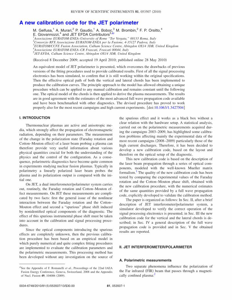
After the vessel, the probing and the reference beam arerecombined �with a recombination quartz plate� and thenthey reach a wire grid which divides the electric field intotwo orthogonal directions that are focused onto two InSbHe-cooled detectors. The schematic layout of the system, forone vertical chord, is shown in Fig. 1.

The Faraday rotation angle is measured on all eightchannels by evaluating the two components of polarizationof the laser beam that passes through the plasma. These mea-

FIG. 1. Schematic of the polarimeter vertical chords.

053507-2 Gelfusa et al. Rev. Sci. Instrum. 81, 053507 �2010�

surements are preceded by an online calibration performedbefore each shot �using half-wave plates�.3,4 In order to mea-sure the Cotton–Mouton angle, a special setup, with initiallinear polarization of the input beam set at 45° with respectto the toroidal field direction �x-axis� for the vertical chan-nels and parallel to the toroidal field for the horizontal chan-nels, has been implemented.

The grid and half-wave plate before the entrance win-dow are used to set the required direction of the linear inputpolarization. In the calibration phase this half-wave plate isrotated before each discharge to simulate the Faraday rota-tion effect.

The amplitudes of the measured beat signals are propor-tional to the orthogonal components of the correspondingelectric field vector amplitudes of the electromagnetic wavein the local coordinate system4 defined by the orientation ofthe wire grid in front of the detectors

p�t� � Ey cos��0t − �� = Ey0 sin · cos��0t − �� , �3�

i�t� � Ex cos��0t� = Ex0 cos · cos��0t� , �4�

where �0 is the modulation frequency �100 kHz� obtained bya rotating grating wheel, � is the phase shift between theorthogonal components, Ex and Ey are the components of theelectrical vector, and =0+ with 0=45°. In presence ofplasma represents the Faraday angle; during the calibrationit is equal to twice the rotation angle of the half-wave plate.

The amplified signals are sent to a phase sensitive elec-tronic module to produce four additional signals that are sentto the data acquisition system.

C. Signal processing electronics

The present electronics used to process data from thedetectors of the JET FIR polarimeter has been commissionedin 2002. Since in the past years the diagnostic has been con-figured for measuring routinely both the Faraday rotationeffect and the Cotton–Mouton effect with a different opticalsetup, it becomes important to check the performance of theanalog phase sensitive electronics.5–7

The main operations performed by the analog electronicsof the polarimeter have been implemented via software usingboth SIMULINK and MATLAB. This allows an accurate charac-terization of the instrument and an assessment of the qualityof the provided measurements. The detected signals �i�t� andp�t�� are processed by analog phase sensitive electronics toobtain the following measurements: RMS, RMP, PSP, andPSD:

RMS = �i�t� � i�t�� , �5�

RMP = �i��t� � i��t�� , �6�

PSD = �i�t� � p�t�� , �7�

PSP = �i��t� � p�t�� , �8�

where i��t��sin��0t� is generated by shifting of 90° thephase of the i�t� signal.

These four signals are processed by a code to obtain thetwo ratios R and R� which are related to polarimetric param-eters of the radiation after the plasma

R =PSD

RMS= C−1 tan�� · cos � , �9�

R� =PSP

�RMS · RMP= C−1 tan�� · sin � , �10�

where C is a calibration factor.Given the two ratio R and R�, the main parameters of the

electrical vector of the polarized radiation can be derived

• the phase shift

� = arctagR�

R= �0 + � , �11�

where �0 is the phase shift between the two signals inabsence of plasma, while � represents the angle intro-duced by the Cotton–Mouton effect.

• the ratio between the orthogonal components of theelectrical vector

R2 + R�2 = C−2 tan2 ⇒ tan2 = C2�R2 + R�2� . �12�

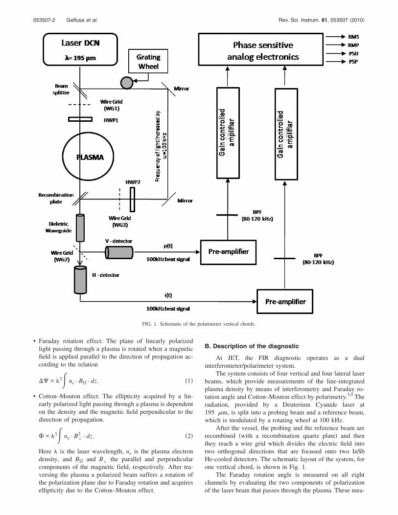
The optical properties of the polarized light, polarizationangle � �, and ellipticity ��=tan �� can be derived usingthe well known identities which relate the electrical pa-rameters to the geometrical ones

tan�2 � = tan�2�cos � , �13�

sin�2�� = sin�2�sin � . �14�

The parameter is the polarization angle between the majoraxis of the polarization ellipse �see Fig. 2� and the referencex-axis; the parameter � is related to the ellipticity of theradiation.

x

y

Ex, 0

Ey, 0X

ψ

JG09

.327

-2c

FIG. 2. �Color online� The polarization ellipse is often adopted to representthe relation between the electrical and the geometrical parameters of thepolarized radiation.

053507-3 Gelfusa et al. Rev. Sci. Instrum. 81, 053507 �2010�

1. Electronics bench test: hardware setup and dataprocessing

The tests to check the reliability of the electronic cardsused on polarimetry have mainly consisted on acquiring theraw data after the detectors, process them via software, andthen compare the obtained outputs with the ones given by thepolarimeter electronics. The first test has been performedgetting the raw signals after the bandpass filter �80–120 kHz�before the phase analog sensitive detector �see Fig. 1�. Thenthe data have been processed by an electronic simulatorimplemented with SIMULINK. For the second and more recenttest the data have been taken after the detectors, before thebandpass filter. This second set of signals has been analyzedwith a MATLAB code, which implements the bandpass filterand the main operations of the phase sensitive detector �Eq.�5�–�8��.

From Fig. 3 it is clear the good agreement between thesimulated signals and the real ones provided by the electron-ics of the polarimeter. This confirms that the phase sensitivedetector is still working properly within its design param-eters.

III. CALIBRATION PROCEDURE

At JET an online calibration, to link the output voltageof the detectors to the effective Faraday rotation angle, iscarried out, for each chord, before each shot.

Currently, the procedure of calibration is the following:the half-wave plate, located at the entrance of the vacuumvessel �see Fig. 1�, is rotated �via a step motor� of a well-

known angle �� and the phase shift ��� is recorded at eachangle, while the Faraday rotation �2� is equal to twice thehalf-wave plate angle.

Moreover, before each campaign, or when it is neces-sary, a manual calibration is performed. It consists of therotation of the wire grid, located in front of the two detectors,to optimize the signals detected.

Figures 4 and 5 show examples of the calibration curvesfor the vertical chord no. 3. Figure 4 represents the Faradayangle as function of the time. Figure 5 shows the phase shiftversus the half-wave plate rotation.

3 5 7 9 11 130

0.2

0.4

0.6

0.8

1# 79338

Time [s]

RMSnorm

ExpCalc

3 5 7 9 11 130

0.2

0.4

0.6

0.8

1

Time [s]

PSDnorm

ExpCalc

3 5 7 9 11 130

0.2

0.4

0.6

0.8

1Ch.3

Time [s]

RMPnorm

ExpCalc

3 5 7 9 11 130

0.2

0.4

0.6

0.8

1

Time [s]

PSPnorm

ExpCalc

FIG. 3. Comparison between the normalized experimental signals RMS, RMP, PSP, PSD �continuous line�, and the estimates of the MATLAB electronicssimulator �dashed line�.

22 23 24 25 26 27 28 29

−15

−10

−5

0

Time (s)

Deg

rees

shot: 77650

FIG. 4. Calibration curve of the Faraday rotation �shot: 77650 chord no. 3�.The error bar on the Faraday rotation is of the order of 0.2°.

053507-4 Gelfusa et al. Rev. Sci. Instrum. 81, 053507 �2010�

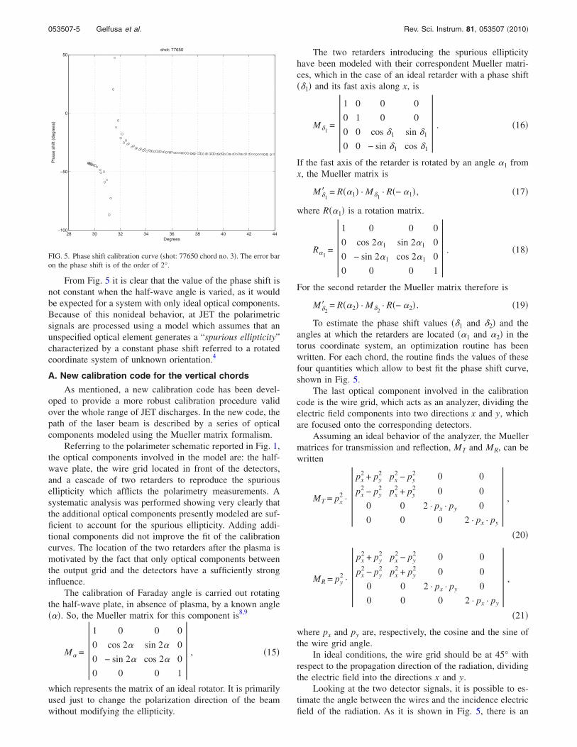
From Fig. 5 it is clear that the value of the phase shift isnot constant when the half-wave angle is varied, as it wouldbe expected for a system with only ideal optical components.Because of this nonideal behavior, at JET the polarimetricsignals are processed using a model which assumes that anunspecified optical element generates a “spurious ellipticity”characterized by a constant phase shift referred to a rotatedcoordinate system of unknown orientation.4

A. New calibration code for the vertical chords

As mentioned, a new calibration code has been devel-oped to provide a more robust calibration procedure validover the whole range of JET discharges. In the new code, thepath of the laser beam is described by a series of opticalcomponents modeled using the Mueller matrix formalism.

Referring to the polarimeter schematic reported in Fig. 1,the optical components involved in the model are: the half-wave plate, the wire grid located in front of the detectors,and a cascade of two retarders to reproduce the spuriousellipticity which afflicts the polarimetry measurements. Asystematic analysis was performed showing very clearly thatthe additional optical components presently modeled are suf-ficient to account for the spurious ellipticity. Adding addi-tional components did not improve the fit of the calibrationcurves. The location of the two retarders after the plasma ismotivated by the fact that only optical components betweenthe output grid and the detectors have a sufficiently stronginfluence.

The calibration of Faraday angle is carried out rotatingthe half-wave plate, in absence of plasma, by a known angle��. So, the Mueller matrix for this component is8,9

M = 1 0 0 0

0 cos 2 sin 2 0

0 − sin 2 cos 2 0

0 0 0 1 , �15�

which represents the matrix of an ideal rotator. It is primarilyused just to change the polarization direction of the beamwithout modifying the ellipticity.

The two retarders introducing the spurious ellipticityhave been modeled with their correspondent Mueller matri-ces, which in the case of an ideal retarder with a phase shift��1� and its fast axis along x, is

M�1=

1 0 0 0

0 1 0 0

0 0 cos �1 sin �1

0 0 − sin �1 cos �1

. �16�

If the fast axis of the retarder is rotated by an angle 1 fromx, the Mueller matrix is

M�1� = R�1� · M�1

· R�− 1� , �17�

where R�1� is a rotation matrix.

R1=

1 0 0 0

0 cos 21 sin 21 0

0 − sin 21 cos 21 0

0 0 0 1 . �18�

For the second retarder the Mueller matrix therefore is

M�2� = R�2� · M�2

· R�− 2� . �19�

To estimate the phase shift values ��1 and �2� and theangles at which the retarders are located �1 and 2� in thetorus coordinate system, an optimization routine has beenwritten. For each chord, the routine finds the values of thesefour quantities which allow to best fit the phase shift curve,shown in Fig. 5.

The last optical component involved in the calibrationcode is the wire grid, which acts as an analyzer, dividing theelectric field components into two directions x and y, whichare focused onto the corresponding detectors.

Assuming an ideal behavior of the analyzer, the Muellermatrices for transmission and reflection, MT and MR, can bewritten

MT = px2 ·

px2 + py

2 px2 − py

2 0 0

px2 − py

2 px2 + py

2 0 0

0 0 2 · px · py 0

0 0 0 2 · px · py

,

�20�

MR = py2 ·

px2 + py

2 px2 − py

2 0 0

px2 − py

2 px2 + py

2 0 0

0 0 2 · px · py 0

0 0 0 2 · px · py

,

�21�

where px and py are, respectively, the cosine and the sine ofthe wire grid angle.

In ideal conditions, the wire grid should be at 45° withrespect to the propagation direction of the radiation, dividingthe electric field into the directions x and y.

Looking at the two detector signals, it is possible to es-timate the angle between the wires and the incidence electricfield of the radiation. As it is shown in Fig. 5, there is an

28 30 32 34 36 38 40 42 44−100

−50

0

50

Degrees

Pha

sesh

ift(d

egre

es)

shot: 77650

FIG. 5. Phase shift calibration curve �shot: 77650 chord no. 3�. The error baron the phase shift is of the order of 2°.

053507-5 Gelfusa et al. Rev. Sci. Instrum. 81, 053507 �2010�

angle of the polarization for which the phase shift diverges to��. Since this corresponds to a polarization for which the Rsignal equals zero and therefore p�t� signal equals zero, itmeans that all the radiation is collected by the i�t� detector.This condition is verified when the wires are parallel to thedirection of p�t� signal. Then the position of the wire withrespect to the incidence electric field can be estimated as

WG2 = 90 − 0. �22�

After this component, the laser beam is divided in two partsand the corresponding Stokes vectors are given by

S�1,R = MR · M�2� · M�1

� · M · S�0, �23�

S�1,T = MT · M�2� · M�1

� · M · S�0. �24�

The final Stokes vector �S�1� is the combination of these twoStokes vectors.

Therefore, it is possible to know the polarization angleand the phase shift, given by

=1

2arctagS2

S1� , �25�

� = arctagS3

S2� , �26�

where S1, S2, and S3 are the component of the final Stokesvector �S�1�.

These parameters are linked to the Faraday rotationangle ��� and to the Cotton–Mouton effect ��� by

� = − 0, �27�

� = � − �0. �28�

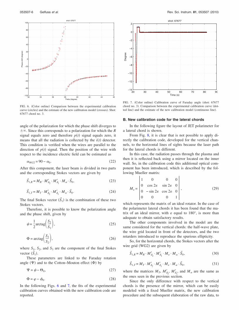
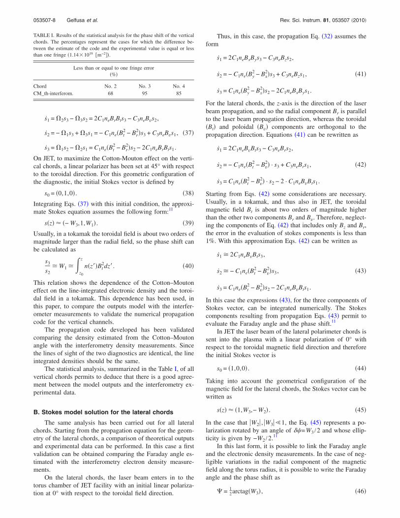
In the following Figs. 6 and 7, the fits of the experimentalcalibration curves obtained with the new calibration code arereported.

B. New calibration code for the lateral chords

In the following figure the layout of JET polarimeter fora lateral chord is shown.

From Fig. 8, it is clear that is not possible to apply di-rectly the calibration code, developed for the vertical chan-nels, to the horizontal lines of sights because the laser pathfor the lateral chords is different.

In this case, the radiation passes through the plasma andthen it is reflected back using a mirror located on the innerwall. So, in the calibration code this additional optical com-ponent has been introduced, which is described by the fol-lowing Mueller matrix:

M� = 1 0 0 0

0 cos 2� sin 2� 0

0 − sin 2� cos 2� 0

0 0 0 1 , �29�

which represents the matrix of an ideal rotator. In the case ofthe polarimeter lateral chords it has been found that the ma-trix of an ideal mirror, with � equal to 180°, is more thanadequate to obtain satisfactory results.

The other components involved in the model are thesame considered for the vertical chords: the half-wave plate,the wire grid located in front of the detectors, and the tworetarders introduced to reproduce the spurious ellipticity.

So, for the horizontal chords, the Stokes vectors after thewire grid �WG2� are given by

S�1,R = MR · M�2� · M�1

� · M� · M · S�0, �30�

S�1,T = MT · M�2� · M�1

� · M� · M · S�0, �31�

where the matrices MT, M�2� , M�1

� , and M are the same asthe ones seen in the previous section.

Since the only difference with respect to the verticalchords is the presence of the mirror, which can be easilymodeled with a fixed Mueller matrix, the new calibrationprocedure and the subsequent elaboration of the raw data, to

32 34 36 38 40 42 44 46−100

−80

−60

−40

−20

0

20

40

60

80

100

Theta (degree)

Pha

sesh

ift(d

egre

e)shot: 67677

FIG. 6. �Color online� Comparison between the experimental calibrationcurve �circles� and the estimate of the new calibration model �crosses�. Shot:67677 chord no. 3.

20 30 40 50 60 70 80 90−14

−12

−10

−8

−6

−4

−2

0

2

Time (s)

Deg

ree

shot: 67677

FIG. 7. �Color online� Calibration curve of Faraday angle �shot: 67677chord no. 3�. Comparison between the experimental calibration curve �dot-ted line� and the estimate of the new calibration model �continuous line�.

053507-6 Gelfusa et al. Rev. Sci. Instrum. 81, 053507 �2010�

evaluate the Faraday rotation and the phase shift angle, arethe same as for the vertical channels. Again only four quan-tities �the phase shift values �1 and �2 and the angles atwhich the retarders are located 1 and 2 in the torus coor-dinate system� have to be determined with a series of scans.

IV. THE NUMERICAL CODE TO SIMULATETHE EVOLUTION OF THE LASER BEAMPOLARIZATION STATE

To confirm the validity of the polarimeter optical model,developed to interpret the calibration data, a numerical codehas been implemented, which calculates the evolution of thestate of polarization of a laser beam crossing JET plasmas.This code is based on the Stokes formalism and has beenparticularized for both the horizontal and the vertical chordsof JET polarimeter. Starting from the Lidar Thomson scatter-ing density profiles and the equilibrium magnetic field asinput, this code gives as output the Faraday rotation angleand the Cotton–Mouton effect. The main equations imple-mented in the code and the basic validation of the results arereported in this section.

As it is well known,10,11 the radiation propagating in amagnetized plasma in the absence of dissipation is describedby the vector equation8,12

ds�

dz= �� � s� , �32�

where the � vector is expressed as

�� = ka��1,�2,�3� �33�

and the three components are equal to

�1 = C1ne�Bx2 − By

2� ,

�2 = 2 · C1neBxBy , �34�

�3 = C3neBz,

where Bx�z�, By�z�, and Bz�z� are the magnetic field compo-nents expressed along the laser beam propagation direction�z�, ne is the electronic density �m−3�, C1=1.74�10−22 and

C3=2�10−20 are constants �calculated for the laser wave-length of 195 �m of JET polarimeter�, and Z=z /ka is thenormalized coordinate with respect to the vertical position zof the chord number i, with k the elongation and a the minusradius of the tokamak.13

Then, using Eqs. �34�, the propagation equation can bewritten as

s1 = �2s3 − �3s2 = 2C1neBxBys3 − C3neBzs2,

s2 = − �1s3 + �3s1 = − C1ne�Bx2 − By

2�s3 + C3neBzs1, �35�

s3 = �1s2 − �2s1 = C1ne�Bx2 − By

2�s2 − 2C1neBxBys1.

The evaluation of the vector �� =ka��1 ,�2 ,�3� is performedin this work using the electron density profile measured bythe Lidar Thomson scattering, while the magnetic field isevaluated using the equilibrium reconstruction of Equilib-rium Fitting with only the magnetic measurements.

A. Stokes model solution for the vertical chords

In the case of the vertical chords, the laser beam propa-gates vertically in a poloidal plane of JET. In this configura-tion the toroidal magnetic field �B� t� is perpendicular to thisplane and then it is possible to write Eqs. �34� in the follow-ing way:

�1 = C1ne�Br2 − Bt

2� ,

�2 = 2 · C1neBrBt, �36�

�3 = C3neBv,

where Br is radial component of the magnetic field, orthogo-nal to the propagation direction, Bt the toroidal component ofthe magnetic field, and Bv is the magnetic field along thepropagation direction, the vertical axis in the case of thisconfiguration.

Under these conditions Eqs. �35� can be written as10

Alcoholλ= 119µ m

Laser DCNλ= 195µ m

V - detector

p(t)

H - detectori(t)

WG2

WG1

M

M M

LEGEND

MHWPBSRPGW

: Mirror: Half-Wave Plate: Beam Splitter: Recombination Plate: Grating Wheel

MM

M M

M

MM

M

BS

BSBSHWP

100kHz

HWP

HWP

5kHzGW

GWBS

BS

MM

RP

JG09

.327

-8c

PLASMA

FIG. 8. �Color online� Schematic of the polarimeter horizontal chords.

053507-7 Gelfusa et al. Rev. Sci. Instrum. 81, 053507 �2010�

s1 = �2s3 − �3s2 = 2C1neBrBts3 − C3neBvs2,

s2 = − �1s3 + �3s1 = − C1ne�Bt2 − Br

2�s3 + C3neBvs1, �37�

s3 = �1s2 − �2s1 = C1ne�Bt2 − Br

2�s2 − 2C1neBrBts1.

On JET, to maximize the Cotton-Mouton effect on the verti-cal chords, a linear polarizer has been set at 45° with respectto the toroidal direction. For this geometric configuration ofthe diagnostic, the initial Stokes vector is defined by

s0 = �0,1,0� . �38�

Integrating Eqs. �37� with this initial condition, the approxi-mate Stokes equation assumes the following form:11

s�z� � �− W3,1,W1� . �39�

Usually, in a tokamak the toroidal field is about two orders ofmagnitude larger than the radial field, so the phase shift canbe calculated as

s3

s2 W1 �

z0

z

n�z��Bt2dz�. �40�

This relation shows the dependence of the Cotton–Moutoneffect on the line-integrated electronic density and the toroi-dal field in a tokamak. This dependence has been used, inthis paper, to compare the outputs model with the interfer-ometer measurements to validate the numerical propagationcode for the vertical channels.

The propagation code developed has been validatedcomparing the density estimated from the Cotton–Moutonangle with the interferometry density measurements. Sincethe lines of sight of the two diagnostics are identical, the lineintegrated densities should be the same.

The statistical analysis, summarized in the Table I, of allvertical chords permits to deduce that there is a good agree-ment between the model outputs and the interferometry ex-perimental data.

B. Stokes model solution for the lateral chords

The same analysis has been carried out for all lateralchords. Starting from the propagation equation for the geom-etry of the lateral chords, a comparison of theoretical outputsand experimental data can be performed. In this case a firstvalidation can be obtained comparing the Faraday angle es-timated with the interferometry electron density measure-ments.

On the lateral chords, the laser beam enters in to thetorus chamber of JET facility with an initial linear polariza-tion at 0° with respect to the toroidal field direction.

Thus, in this case, the propagation Eq. �32� assumes theform

s1 = 2C1neBxBys3 − C3neBzs2,

s2 = − C1ne�By2 − Bx

2�s3 + C3neBzs1, �41�

s3 = C1ne�By2 − Bx

2�s2 − 2C1neBxBys1.

For the lateral chords, the z-axis is the direction of the laserbeam propagation, and so the radial component Br is parallelto the laser beam propagation direction, whereas the toroidal�Bt� and poloidal �Bv� components are orthogonal to thepropagation direction. Equations �41� can be rewritten as

s1 = 2C1neBvBts3 − C3neBrs2,

s2 = − C1ne�Bt2 − Bv

2� · s3 + C3neBrs1, �42�

s3 = C1ne�Bt2 − Bv

2� · s2 − 2 · C1neBvBts1.

Starting from Eqs. �42� some considerations are necessary.Usually, in a tokamak, and thus also in JET, the toroidalmagnetic field Bt is about two orders of magnitude higherthan the other two components Br and Bv. Therefore, neglect-ing the components of Eq. �42� that includes only Bz and Br,the error in the evaluation of stokes components is less than1%. With this approximation Eqs. �42� can be written as

s1 2C1neBvBts3,

s2 − C1ne�Bt2 − Bv

2�s3, �43�

s3 = C1ne�Bt2 − Bv

2�s2 − 2C1neBvBts1.

In this case the expressions �43�, for the three components ofStokes vector, can be integrated numerically. The Stokescomponents resulting from propagation Eqs. �43� permit toevaluate the Faraday angle and the phase shift.11

In JET the laser beam of the lateral polarimeter chords issent into the plasma with a linear polarization of 0° withrespect to the toroidal magnetic field direction and thereforethe initial Stokes vector is

s0 = �1,0,0� . �44�

Taking into account the geometrical configuration of themagnetic field for the lateral chords, the Stokes vector can bewritten as

s�z� � �1,W3,− W2� . �45�

In the case that �W2� , �W3��1, the Eq. �45� represents a po-larization rotated by an angle of � =W3 /2 and whose ellip-ticity is given by −W2 /2.11

In this last form, it is possible to link the Faraday angleand the electronic density measurements. In the case of neg-ligible variations in the radial component of the magneticfield along the torus radius, it is possible to write the Faradayangle and the phase shift as

� = 12arctag�W3� , �46�

TABLE I. Results of the statistical analysis for the phase shift of the verticalchords. The percentages represent the cases for which the difference be-tween the estimate of the code and the experimental value is equal or lessthan one fringe �1.14�1019 �m−2��.

Less than or equal to one fringe error�%�

Chord No. 2 No. 3 No. 4CM_th-interferom. 68 95 85

053507-8 Gelfusa et al. Rev. Sci. Instrum. 81, 053507 �2010�

� = arctag�− W2� . �47�

Since W3=C3�z0

z n�z� · �Br�dz the Faraday angle � is propor-tional to the line integral of the electronic density and to theradial magnetic field Br.

The numerical solutions of Eq. �42�, or of the approxi-mated form �43�, for the lateral chords are in acceptableagreement with data of the Faraday angle and with the inter-ferometer measurements. The summary of the statisticalanalysis on all lateral chords is given in Table II. In this casethe shots available for the statistical analysis are smaller thanthe vertical ones due to hardware problems with the lateralviews.

V. APPLICATION TO THE PLASMA MEASUREMENTS

Once obtained the calibration curves for the Faraday ro-tation and the phase shift, the experimental signals withplasma have been analyzed applying the new calibrationcode.

Starting from the raw data acquired, RMS, RMP, PSP,and PSD, one can obtain the components of Stokes vector,8

which describes the polarization state of the beam passesthrough all the optical components and the plasma, using thefollowing equations �see Sec. II�:

RMS = 12EH,0

2 , �48�

RMP = 12EH,0�2 , �49�

PSD = 12EH,0� · EV,0 cos � , �50�

PSP = 12EH,0 · EV,0 cos � , �51�

where the EH,0 and EV,0 are the electric field componentsmeasured, respectively, with the H-detector and theV-detector �see Fig. 1� and � is the phase shift between them.

Since the position of the output wire grid could be ro-tated with respect to the original reference axes, a rotation ofits output components has to be performed to express themin the right coordinate system. To this purpose the electricfield components after the wire grid analyzer have to be ex-pressed by means of the following transformations:

Ex = · EH,0 + � · EV,0, �52�

Ey = − � · EH,0 + · EV,0, �53�

where and � are, respectively, the cosine and the sine ofthe wire grid angle in the torus coordinate system. Oncederived the components of the electric field at the exit of theplasma, the final Stokes vector �S�1� can be calculated.8

Hence, applying the calibration matrices to S�1, it is pos-sible to evaluate the plasma effects on the initial polarizationstate of laser beam, according to

S�1 = M�2� · M�1

� · M · Mplasma · S�0 �54�

and thus

M−1 · M�1

�−1 · M�2�−1 · S�1 = Mplasma · S�0 �55�

for the vertical chords. For the horizontal chords the relationis

M−1 · M� · M�1

�−1 · M�2�−1 · S�1 = Mplasma · S�0. �56�

After this procedure, the calibration parameter C, due to thesignal processing electronics, is estimated. Since in absenceof plasma the Faraday rotation must be equal to twice thehalf-wave angle, it is easy to find C comparing the experi-mental data �before 40 s� with this curve.

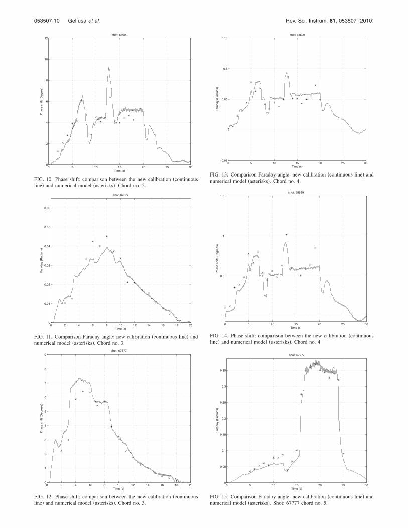
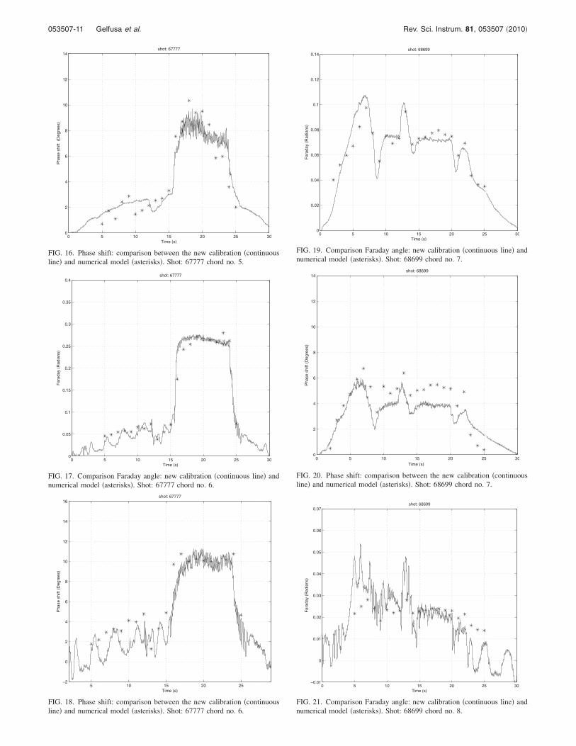
Figure 9 compares the Faraday rotation calculated withthe new calibration code, with the results of a numericalmodel described in Sec. IV �asterisks�. In Fig. 10 the samecomparison for the phase shift is shown. The new calibrationis in good agreement with the numerical solution. Figures11–22 depict the results obtained for some shots acquiredduring the 2003–2007 experimental campaigns to show howthe developed algorithm works satisfactorily for all chords.

Given the good results obtained for the earlier cam-paigns, the new calibration code has been applied to theshots performed during 2008–2009 and, also in this case, thecomparison between the Stokes model outputs and the newcalibration shows a good agreement.

On JET, for the vertical chords, it is easy to evaluate thedensity from the Cotton–Mouton measurements because thetoroidal field �Bt� is largely constant along the line of sight,and thus Eq. �2� can be rewritten as

TABLE II. Statistical analysis, for all lateral chords, of the measurements ofthe electron density. Again the percentages of the estimates in acceptableagreement with the experimental measurements within one fringe are re-ported.

Statistical analysis on 200 shots–one fringe error�%�

Chord No. 5 No. 6 No. 7 No. 8Far_th-interferom 56 64 61 44

0 5 10 15 20 25 30

−0.15

−0.1

−0.05

0

Time (s)

Far

aday

(Rad

ians

)

shot: 68699

FIG. 9. Comparison Faraday angle: new calibration �continuous line� andnumerical model �asterisks�. Chord no. 2.

053507-9 Gelfusa et al. Rev. Sci. Instrum. 81, 053507 �2010�

0 5 10 15 20 25 300

2

4

6

8

10

12

Time (s)

Pha

sesh

ift(D

egre

e)

shot: 68699

FIG. 10. Phase shift: comparison between the new calibration �continuousline� and numerical model �asterisks�. Chord no. 2.

0 2 4 6 8 10 12 14 16 18 200

0.01

0.02

0.03

0.04

0.05

0.06

Time (s)

Far

aday

(Rad

ians

)

shot: 67677

FIG. 11. Comparison Faraday angle: new calibration �continuous line� andnumerical model �asterisks�. Chord no. 3.

0 2 4 6 8 10 12 14 16 18 200

1

2

3

4

5

6

7

8

9

Time (s)

Pha

sesh

ift(D

egre

es)

shot: 67677

FIG. 12. Phase shift: comparison between the new calibration �continuousline� and numerical model �asterisks�. Chord no. 3.

0 5 10 15 20 25 30−0.05

0

0.05

0.1

0.15

Time (s)

Far

aday

(Rad

ians

)

shot: 68699

FIG. 13. Comparison Faraday angle: new calibration �continuous line� andnumerical model �asterisks�. Chord no. 4.

0 5 10 15 20 25 30

0

0.5

1

1.5

Time (s)

Pha

sesh

ift(D

egre

es)

shot: 68699

FIG. 14. Phase shift: comparison between the new calibration �continuousline� and numerical model �asterisks�. Chord no. 4.

0 5 10 15 20 25 300

0.05

0.1

0.15

0.2

0.25

0.3

0.35

Time (s)

Far

aday

(Rad

ians

)

shot: 67777

FIG. 15. Comparison Faraday angle: new calibration �continuous line� andnumerical model �asterisks�. Shot: 67777 chord no. 5.

053507-10 Gelfusa et al. Rev. Sci. Instrum. 81, 053507 �2010�

0 5 10 15 20 25 300

0.05

0.1

0.15

0.2

0.25

0.3

0.35

0.4

Time (s)

Far

aday

(Rad

ians

)

shot: 67777

FIG. 17. Comparison Faraday angle: new calibration �continuous line� andnumerical model �asterisks�. Shot: 67777 chord no. 6.

5 10 15 20 25−2

0

2

4

6

8

10

12

14

16

Time (s)

Pha

sesh

ift(D

egre

es)

shot: 67777

FIG. 18. Phase shift: comparison between the new calibration �continuousline� and numerical model �asterisks�. Shot: 67777 chord no. 6.

0 5 10 15 20 25 300

0.02

0.04

0.06

0.08

0.1

0.12

0.14

Time (s)

Far

aday

(Rad

ians

)

shot: 68699

FIG. 19. Comparison Faraday angle: new calibration �continuous line� andnumerical model �asterisks�. Shot: 68699 chord no. 7.

0 5 10 15 20 25 300

2

4

6

8

10

12

14

Time (s)

Pha

sesh

ift(D

egre

es)

shot: 68699

FIG. 20. Phase shift: comparison between the new calibration �continuousline� and numerical model �asterisks�. Shot: 68699 chord no. 7.

0 5 10 15 20 25 300

2

4

6

8

10

12

14

Time (s)

Pha

sesh

ift(D

egre

es)

shot: 67777

FIG. 16. Phase shift: comparison between the new calibration �continuousline� and numerical model �asterisks�. Shot: 67777 chord no. 5.

0 5 10 15 20 25 30−0.01

0

0.01

0.02

0.03

0.04

0.05

0.06

0.07

Time (s)

Far

aday

(Rad

ians

)

shot: 68699

FIG. 21. Comparison Faraday angle: new calibration �continuous line� andnumerical model �asterisks�. Shot: 68699 chord no. 8.

053507-11 Gelfusa et al. Rev. Sci. Instrum. 81, 053507 �2010�

� = k · �3 · Bt2 ·� ne · dz �57�

and therefore the line-integrated electron density �ne� can bedirectly obtained

� ne · dz =�

k · �3 · Bt2 , �58�

where k is a constant.In the Figs. 23–25, the density calculated applying the

new calibration code, for the vertical chords, is reported. Thecurve is compared with the computational model output andwith the density measurement of the interferometer.

As it is clear, using the new calibration the density cal-culated with the polarimeter and with the interferometer arein good agreement.

VI. CONCLUSIONS

JET polarimeter has been analyzed to understand and tosolve the problems posed by the spurious ellipticity inducedby the instrument optical components. Two analyses havebeen performed:

�1� check of the signal processing electronics to exclude ad-ditional anomalous behaviors;

�2� development of a new calibration code.

A simulator has been developed to verify the proper op-eration of the electronics. The analysis shows a very goodagreement between the simulation outputs and the experi-mental data. Therefore, we can conclude that the signal pro-cessing electronics is still working within its design param-eters.

After this analysis, a new calibration code has been writ-ten and tested for many shots acquired in different cam-

0 5 10 15 20 25 30

−5

0

5

10

15

20

25

Time (s)

Pha

sesh

ift(D

egre

es)

shot: 68699

FIG. 22. Phase shift: comparison between the new calibration �continuousline� and numerical model �asterisks�. Shot: 68699 chord no. 8.

0 5 10 15 20 25−15

−10

−5

0

5

10

15

20

Time (s)

Den

sity

(*10

19/m

2 )

shot: 77650

FIG. 23. �Color� Comparison between the density with the new calibration�blue line�, the interferometer density �magenta line�, the numerical model�asterisk�, and the old calibration �red line�. Shot: 77650 chord no. 2.

5 10 15 20 25−4

−2

0

2

4

6

8

10

12

14

16

18

Time (s)

Den

sity

(*10

20/m

2 )

shot: 79388

FIG. 24. �Color� Comparison between the density with the new calibration�blue line�, the interferometer density �magenta line�, the numerical model�asterisks�, and the old calibration �red line�. Shot: 79388 chord no. 3.

2 4 6 8 10 12 14 16 18−2

−1

0

1

2

3

4

Time (s)

Den

sity

(*10

19/m

2 )

shot: 78058

FIG. 25. �Color� Comparison between the density with the new calibration�blue line�, the interferometer density �magenta line�, the numerical model�asterisks�, and the old calibration �red line�. Shot: 78058 chord no. 4.

053507-12 Gelfusa et al. Rev. Sci. Instrum. 81, 053507 �2010�

paigns. The experimental data, calibrated with this code,have been compared with the rigorous numerical solution ofthe Stokes equations. The obtained results show that the twoestimates are in good agreement for both the Faraday rota-tion and the Cotton–Mouton effect. Moreover, starting fromthe phase shift obtained with this new code, the electrondensity has been evaluated for the vertical channels and com-pared with the density measured by the interferometer. Thecomparison with the experimental measurements confirmsthe quality of the developed calibration procedure.

ACKNOWLEDGMENTS

This work, supported by the European Communities un-der the contract of Association between EURATOM andENEA, was carried out under the framework of the EuropeanFusion Development Agreement. The views and opinions ex-

pressed herein do not necessarily reflect those of the Euro-pean Commission.

1 D. Goldstein, Polarized Light �CRC, Boca Raton, 2003�.2 F. De Marco and S. Segre, Plasma Phys. 14, 245 �1972�.3 K. Guenther, Proceedings of the 31st EPS, 2004, P5–172.4 K. Guenther, Plasma Phys. Controlled Fusion 46, 1423 �2004�.5 C. Brault, CEA Cadarache, Internal Mission report, March 2009.6 M. Gelfusa, M. Brombin, P. Gaudio, A. Boboc, A. Murari, and F. P.Orsitto, “Modelling of the signal processing electronics of JETinterferometer-polarimeter,” Nucl. Instrum. Methods Phys. Res. �in press�.

7 See http://www.tina.com/English/tina for the detailed description of thesoftware package designed to simulate electronic circuits.

8 M. Born and E. Wolf, Principles of Optics �Pergamon, Oxford, 1980�.9 D. S. Kliger, J. W. Lewis, and C. E. Randall, Polarized Light in Opticsand Spectroscopy �Academic, San Diego, 1990�.

10 S. E. Segre, Plasma Phys. Controlled Fusion 35, 1261 �1993�.11 S. E. Segre, Plasma Phys. Controlled Fusion 41, R57 �1999�.12 F. De Marco and S. E. Segre, Opt. Commun. 23, 125 �1977�.13 F. P. Orsitto, A. Boboc, C. Mazzotta, E. Giovannozzi, and L. Zabeo,

Plasma Phys. Controlled Fusion 50, 115009 �2008�.

053507-13 Gelfusa et al. Rev. Sci. Instrum. 81, 053507 �2010�