Agricultural and Forest Meteorology 100 (2000) 213–230

A model to estimate the temperature of a maize apex frommeteorological data

Lydie Guilionia, Pierre Cellierb,∗, Françoise Rugetc, Bernard Nicoullaudd,Raymond Bonhommeb

a Laboratoire d’ Ecophysiologie des Plantes sous Stress Environnementaux, INRA-AGRO.M, UFR Agronomie et Bioclimatologie, 2, placeViala, 34060 Montpellier Cedex 02, France

b INRA, Unité de Recherche en Bioclimatologie, F78850 Thiverval-Grignon, Francec INRA, Unité de Recherche en Bioclimatologie, 84914 Avignon Cedex 9, France

d INRA, Service d’Etude des Sols et de la Carte Pédologique de France, Ardon, 45160 Olivet, France

Received 16 September 1998; received in revised form 23 July 1999; accepted 17 September 1999

Abstract

During early growth, when the apical meristem of a maize plant is close to the soil surface, its temperature may be verydifferent from air temperature. A model is proposed to estimate apex temperature from meteorological data, when the leafarea index is less than 0.5. This model is based on the energy balance of the apical meristem, considered as a vertical cylinderclose to the soil surface, called ‘apex’. Soil surface temperature was calculated from an energy and water balance of thesoil. Input data were hourly standard meteorological data and soil texture. Stomatal conductance was calculated from solarradiation and water vapor deficit.

Five field experiments with different soil and climatic conditions were conducted to calibrate and validate the model. Theroughness length of the soil surface was used as a calibrating factor. The selected value was 0.3 mm, and was used on alldatasets. The agreement between observed and calculated apex temperatures was fairly good, with residual standard deviationsbetween 0.8 and 1.9 K in five experiments, while apex temperature was generally higher than air temperature at screen levelby more than 5–7 K during the day. This study showed that the main problem to overcome in estimating apex temperature,is to calculate air temperature at apex height, i.e. at several centimeters from the soil surface. This requires development ofprecise soil surface temperature models. ©2000 Elsevier Science B.V. All rights reserved.

Keywords:Maize; Meristematic zone; Temperature; Prediction; Energy balance; Meteorological data

1. Introduction

Temperature has a major influence on plant growthand particularly on development rates. Many studieshave shown that leaf initiation, leaf appearance andelongation are strongly related to temperature (Watts,

∗ Corresponding author. Tel.:+33-1-30-81-55-55;fax: +33-1-30-81-55-63.E-mail address:cellier@bcgn.grignon.inra.fr (P. Cellier).

1972a; Warrington and Kanemasu, 1983 in maize;Gallagher, 1979 in wheat and barley; Ong, 1983 inpearl millet). De Reaumur first suggested in 1735 (DeReaumur, 1735) that the duration of particular stagesof growth was directly related to temperature and thatthis duration for a particular species could be pre-dicted using the sum of mean daily air temperature.This way of normalizing time with temperature, thethermal time, in order to predict the plant developmentrates has been widely used in this century (Durand

0168-1923/00/$ – see front matter ©2000 Elsevier Science B.V. All rights reserved.PII: S0168-1923(99)00130-6

214 L. Guilioni et al. / Agricultural and Forest Meteorology 100 (2000) 213–230

et al., 1982; Ritchie and NeSmith, 1991). The conceptof thermal time assumes a strong correlation betweenair temperature and that sensed by the plant (Durandet al., 1982). But in maize, like in many monocot cropplants, the specific locations where temperature influ-ences development — i.e. the zones where cell divi-sion and expansion are occurring (Kleinendorst andBrouwer, 1970; Watts, 1972b; Peacock, 1975) — areclose to the soil surface during early growth. In theseconditions, the development rates (leaf initiation, leafappearance or reproductive initiation rate) are not ac-curately related to air temperature (Beauchamp andLathwell, 1966; Brouwer et al., 1970; Aston, 1987).Duburcq et al. (1983) have shown that the develop-ment rate of maize until male floral initiation was bet-ter related to soil temperature than to air temperature.Swan et al. (1987) found that the development rate ofmaize was best described using soil temperature untilthe sixth leaf was fully developed. More recently, Shar-ratt (1991) over barley and Bollero et al. (1996) overmaize observed different development rates under dif-ferent controlled soil temperatures. Moreover, lookingdirectly at plant temperature, either in growth-chamberor in field conditions, Ben Haj Salah and Tardieu(1996) observed that leaf elongation rate was corre-lated better with meristematic apex temperature thanwith air temperature. Similarly, Jamieson et al. (1995)calculated thermal time based on plant temperature.They concluded that ‘a model of leaf appearance basedon near surface temperature and canopy temperaturegave superior prediction than others based on air tem-perature’.

Cellier et al. (1993) have shown that the tempera-ture of the meristem was significantly different fromboth air and soil surface temperatures. The differencesbetween air temperature at screen height and meris-tem temperature reached almost 6 K for a daytimeaverage, which means that hourly values were muchlarger. Thus, accounting for the influence of tempera-ture on growth and development should be improvedby using the actual temperature of the extension zones.Beauchamp and Torrance (1969) proposed a model forestimating the internal temperature of a young maizeplant. The maize stem was represented as a verticalcylindrical bar with one end in the soil considered asan infinite source of heat. This model overestimatedthe temperature of the plant certainly because neitherthe circulation of water in the stem nor the transpi-

ration was considered. Cellier et al. (1993) proposeda model — based on a energy balance equation —to predict the differences between air and meristemtemperatures from standard meteorological data dur-ing the early growth of a maize plant. However, thismodel presented some limits. The radiation balanceneglected the shade of leaves, and in the absence ofany references, the stomatal conductance of the meris-tematic zones was a fitting parameter. Furthermore, theoutput data are averages of day and night temperatureswith no way to estimate maximum or minimum whichmay be the most relevant temperatures for explainingdifferences in development rate (Weaich et al., 1996).

In this paper, we proposed a model based also on anenergy balance approach, for estimating the temper-ature of the extension zones of a young maize. Thismodel works at hourly time steps, from standard me-teorological data. The main improvements comparedto the original model of Cellier et al. (1993) are relatedto the radiation balance, the stomatal conductance pa-rameterization and the air temperature profile near thesoil surface.

2. Methods

2.1. Model

The extension zones (consisting of both leaves andapical meristem) which are often called ‘pseudo-stem’,will be referred to as ‘apex’ in the following text. Theapex temperature, denotedTm, is calculated from theenergy balance of the apex, considered as a verticalcylinder whose temperature is considered as uniformand homogeneous over the time steps of the model.This model aims at estimating the apex temperaturefor such uses as integration in crop growth modelsinstead of the air temperature. To set up such an op-erational model, a compromise needs to be found be-tween a realistic description of the energy exchangesbased on mathematical expressions and the use ofreadily available data and parameters. The amount ofcalculations is no longer a problem today, and a largeamount of work has been done in physical ecologyto relate energy exchanges to plants and meteoro-logical parameters and variables. Consequently, themain problem for such a model is to use only readilyavailable data.

L. Guilioni et al. / Agricultural and Forest Meteorology 100 (2000) 213–230 215

During daylight, the main energy input to the apex isradiation, both solar and long-wave radiation. A part ofthis energy is released by evaporation through stomata.If apex temperature is different from air temperature atthe same height, energy may be absorbed or released assensible heat by convection. Moreover, energy may betransferred through the apex in a vertical direction byconvection and/or conduction. During the night, mostof these fluxes change sign. The radiation balance isnegative, and water vapor may condense on the apex.

The energy balance of the apex can be written

Rnm + Gm + Hm + λEm = 0 (1)

whereRnm is the net radiation,Hm andλEm are thesensible heat and the latent heat fluxes between theapex and the surrounding air.Gm is the transportof heat along the apex by conduction through theplant tissues or convection by sap flow. The valuesof the parameters mentioned in the following equa-tions are summarized in Table 1, and the notationsare recapitulated in Appendix A. All the input dataof the model are (1) data measured by a standardmeteorological station and (2) plant characteristicswith fixed values. The model calculates apex tem-perature over short time steps (1 h or less). It is theonly time step for which the hypothesis of stationarityof the energy balance and several parameterizationssuch as that of stomatal conductance or temperatureprofiles (see below) are valid. This model runs inthe early growth stages, when leaf area index (LAI)is less than 0.5 m2 m−2. This limitation is imposedby the parameterization of both radiative and con-vective schemes. With taller crops a more complex

Table 1Values and origin of the constants used in the model

Symbol Significance Value Unit Source

am apex albedo 0.29 – Davies and Buttimor (1969)dm apex diameter 0.01 m Experimentgsm minimum stomatal conductance 0.1 mm s−1 Bethenod and Tardieu (1990)gsM maximum stomatal conductance 5 mm s−1 Bethenod and Tardieu (1990)KPAR coefficient of Eq. (10) 379 mmol m−2 s−1 Olioso et al. (1995)KD coefficient of Eq. (10) 61 hPa Olioso et al. (1995)zo roughness length 0.3 mm Fittedzm apex height 20 mm Experimentα coefficient of Eq. (4d) 0.46 – Weiss and Norman (1985)εm apex emissivity 1.00 –τNIR leaf near infrared transmissivity 0.20 –τPAR leaf PAR transmissivity 0.03 – Fitted

radiative transfer model should be used, includingsome plant characteristics (LAI, leaf angles,. . . ).For convective processes, wind and temperature pro-files in the canopy would be too strongly modifiedcompared to classical profiles observed over bare soil.

The energy balance is based on the description of thelocal energy exchanges depending on microclimaticvariables at apex height. More precisely, the model es-timates the temperature difference between the apexand the air at apex height. This means that estimatingair temperature at apex height is a determining step inthis apex temperature model. This is especially diffi-cult in early stages of development. Indeed, the soilsurface is only sparsely covered with vegetation, andwhen the weather is dry, the temperature gradient nearthe soil surface can be very steep. Consequently, mod-eling apex temperature can be divided into two steps:the first one consists in determining the air tempera-ture at apex height, i.e. the difference in air tempera-ture between screen height and apex height, and thesecond one consists in estimating the temperature dif-ference between the apex and the surrounding air. Thefirst step requires knowledge of micrometeorologicalconditions at field scale. The second needs to accountfor local characteristics of the microclimate or of sur-face conditions near the apex. The importance of bothsteps might be very variable depending on the part ofthe vegetation being considered. For a shaded evapo-rating organ, the temperature difference between theorgan and the air (second step) is expected to be smallbecause the organ receives low energy, and a largefraction of it can be dissipated into latent heat. For anorgan directly exposed to solar radiation (e.g. wheat

216 L. Guilioni et al. / Agricultural and Forest Meteorology 100 (2000) 213–230

ear, pea flower, top leaves) the temperature differenceshould be much larger, especially in the case of anon-evaporating organ (e.g. a bud before bud burst).On the other hand, the temperature difference betweenthe air at screen height and the air surrounding theapex (first step) can also be very variable accordingto the field conditions: from several degrees or tens ofdegrees over a bare dry soil (Garratt, 1988; Cellier etal., 1996) to several tenths of degrees over an evap-orating vegetation or a wet soil. Consequently, bothtemperature differences must be considered to build amodel adapted to a wide range of vegetation and me-teorological conditions and to be able to analyze whatdetermines plant temperature.

2.1.1. Temperature and wind speed profiles abovethe soil surface

Due to interactions between free and forced convec-tion air temperature and wind speed profiles cannot bedetermined independently from each other. Moreover,both air temperatureTam, and wind speed,Um, at apexheight are required in some fluxes of the energy bal-ance equation. Wind speed and air temperature varia-tion with height are generally described by using theflux-gradient relationships given by Dyer and Hicks(1970)

u(z) = u∗k

[ln

(z

zo

)− 9M

(z − zo

L

)](2)

T (z) − To = T∗k

[ln

(z

zoh

)− 9H

(z − zoh

L

)](3)

whereu(z) andT(z) are the wind speed and air temper-ature at heightz; u∗ is friction velocity,T∗ a scale tem-perature, andzo andzoh are the roughness lengths formomentum and heat transfer. As generally assumed,zoh was taken equal to 0.1zo (Brutsaert, 1982). TheMonin–Obukhov length,L, is related tou∗ andT∗ byL = T/kg u2∗/T∗. The stability functions9M and9Haccount for the effects of vertical temperature gradienton convective transfer (Dyer and Hicks, 1970). Theirexpressions were derived by Paulson (1970).

Determining the wind and temperature profiles re-quires calculation ofu∗, T∗ andL using Eq. (3) andanalogous equations. For this, the air temperature atzoh, To, must be determined. This was done using anenergy balance of the soil surface, including a soil sur-face water balance as described in Appendix B. This

method makes it possible to account for the variationsof soil surface temperature due to meteorological con-ditions and soil wetting/drying according to the cli-matic factors and capillary water transfer in the topsoil. The height whereTam andUm are calculated asthat of the apex,zm was taken as 0.02 m.

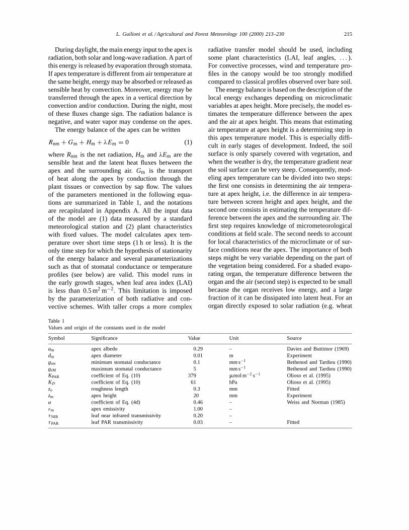
2.1.2. Radiation balanceThe radiation balance is divided into short-wave

and long-wave radiation balances. Visual observationshowed that for most of the day, the apex was shad-owed by its own leaves or those of the neighbouringplants in the same row. This is especially true when thesolar elevation is high, i.e. when solar radiation is atthis peak. We could then consider that short-wave radi-ation reaching the apex was either transmitted throughthe leaves or reflected from the soil (Fig. 1). In bothcases, it is diffuse radiation. As leaf transmittance isdifferent for photosynthetically active (PAR) and nearinfrared radiation (NIR), these spectral intervals haveto be considered separately. Moreover, PAR radiationis required for calculating stomatal conductance (seebelow). Due to shadowing by leaves, no directional ef-fect of radiation was considered. Short-wave radiationbalance,RSWm, may then be expressed as

RSWm = (1 − am)(RPARm + RNIRm) (4a)

with

RPARm = (τPAR + as)RPAR (4b)

and

RNIRm = (τNIR + as)RNIR (4c)

wheream andas are the plant and soil albedos. AlsoτPAR andτNIR are the transmittances of leaves in thePAR and near infrared wavelength ranges.RPAR andRNIR are the PAR and NIR inputs over the canopyobtained from the solar radiationRs by

RPAR = αRs (4d)

RNIR = (1 − α)Rs (4e)

Following Weiss and Norman (1985),α was takenequal to 0.46. All radiation components are expressedin units of W m−2. In RPARm andRNIRm the index ‘m’refers to the incident radiation on the apex.

L. Guilioni et al. / Agricultural and Forest Meteorology 100 (2000) 213–230 217

Fig. 1. Schematic representation of the short-wave radiation balance of the apex (Rs, solar radiation;RPAR, RNIR incident PAR and incidentNIR above the crop;RPARm, RNIRm, PAR and NIR at the apex surface;am apex albedo;as soil albedo;τPAR, τNIR, leaf transmissivity forPAR and NIR).

The long-wave radiation balance is written

RLWm = εm(Ram − σT 4m) (5)

The first term on the right-hand-side of Eq. (5),Ram,is the long-wave radiation input from the surround-ing environment (sky, leaves, soil). This flux was ex-pressed as

Ram = σT 4a + σT 4

s

2(6)

whereTa is air temperature (K) measured at screenheight andTs is the soil surface temperature. The firstterm on the right-hand side of Eq. (6) isσT 4

a insteadof atmospheric radiation because it can be consideredthat the apex mainly ‘looks at’ the lower atmosphere atlarge angles from the zenith and maize leaves (whosetemperature is close to air at screen height) at lowangles (Fig. 1). The second term in the right-hand-sideof Eq. (5) represents the long-wave radiation losseslinked to the apex temperature. The apex emissivity,εm, is taken equal to 1.00, as usually done for mostvegetation, and the soil emissivity too.

2.1.3. Sensible heat exchangesThe transfer of sensible heat from the apex to the

surrounding air is considered as proportional to thetemperature difference between the apex and the airat apex height

Hm = ρcpgm(Tm − Tam) (7)

whereTam is air temperature at apex height, andgm isa thermal diffusion conductance. Its value depends onthe wind speed at apex height,Um, and on the apexdiameter,dm. It can be expressed according to theexpression given by Finnigan and Raupach (1987).

gm = 0.54

(Um

dm

)1/2

(8)

Tam andUm were calculated from air temperature andwind speed profiles as previously described.

2.1.4. EvaporationThe transpiration from the apex is mainly regulated

by stomata. It may be expressed in a form similar tothat of the sensible heat flux,

λEm = ρcp

γ

em − eam

1/gv + 1/gs(9)

whereeam is the vapor pressure at apex height andem is the vapor pressure inside substomatal chambersof the leaves which constitute the external face of theapex. It is taken equal to the saturation vapor pres-sure at apex temperature;eam can be calculated froma relationship similar to Eq. (3) where the tempera-ture scale is replaced by a humidity scale determinedfrom the soil evaporation calculated according to the

218 L. Guilioni et al. / Agricultural and Forest Meteorology 100 (2000) 213–230

procedure described in Appendix B;gv is a thermaldiffusion conductance, equal to 0.89gm (Eq. (8)).

The stomatal conductance,gs, is controlled by dif-ferent environmental factors, among which radiation,water vapor pressure deficit, soil water content and at-mospheric carbon dioxide concentration are the mostimportant (Jarvis, 1976). Considering that, just aftersowing, soil water content was rarely a limiting factor,gs was modeled using only a regulation by solar ra-diation and water vapor deficit. The relation proposedby Olioso et al. (1995) was used,

gs = gsm + (gsM − gsm)

[1 − exp

(−QPAR

KPAR

)]

×[1 − D

KD

](10)

wheregsm andgsM are the minimum and maximumconductances (m s−1), D is the water vapor pressureair deficit at apex level;QPAR is RPARm (Eq. (4)), butexpressed inmmol m−2 s−1; KPAR andKD are constantcoefficients given by Olioso et al. (1995) (see Table 1).

2.1.5. Heat flux through the stemUnder daytime conditions, heat is transported from

the underlying warmer ground to the leaves by sapflow through the apex. Temperature measurements be-low and above the apex showed that the amount ofheat transported by this way was less than 10% of thenet radiation in all cases, and their difference, whichrepresents the energy storage by the apex was muchless. Therefore, this flux was neglected.

2.1.6. Calculation of the apex temperatureUsing Eqs. (1) and (4)–(10), the energy balance

equation was solved at each time step using an itera-tive procedure. The iteration of apex temperature wasterminated when the energy balance closed to within1 W m−2. The same approach was used at the sametime to calculate soil surface temperature and watercontent, using Eqs. (B.1)–(B.10). If not available, thesoil water content was initialized to 75% of the fieldcapacity for the surface layer, and to the field capacityfor the deep soil layer. The apex temperatures calcu-lated during the first day were excluded from the anal-ysis so that the results might not be affected by badlyestimated initial soil water contents.

2.2. Field experiments

2.2.1. Field conditionsThis model was calibrated and tested with five

datasets, collected at three sites. Three experimentswere conducted in Grignon, France (48◦51′N, 1◦58′E,altitude 125 m), one in 1990 and two in 1993, overa 1.4 ha maize field (Zea maysL.) of the INRA ex-perimental station, with a clay-loam soil. The albedowas 0.20 under dry conditions, and decreased to 0.15after rainfall. In 1990, the maize was sown on 4 May(day of year (DOY) 124) and the measurements ofapex temperatures were made from 23 May (DOY143) to 30 May (DOY 150). In 1993, two sub-plots of40 m× 40 m (called A and B) were sown in the samefield at two different dates in order to get different cli-matic conditions, especially temperature. The maizewas sown on 7 May 1993 on plot A and on 9 June onplot B. Apex temperatures were measured from 15 to29 June for A and from 4 to 15 July for B. The threeexperiments performed in Grignon will be referred toasGrignon90, Grignon93A, andGrignon93B.

Two other experiments were conducted in 1992 intwo farmers’ fields near Pithiviers, France (48◦08′N,2◦13′E, altitude 120 m). The first (called ‘Brosses’)was on a calcareous loamy soil with small stones andthe second (called ‘Lacour’) was on a loamy sand soil.The apex temperatures were measured from 22 to 29May. Over both fields, the albedo was 0.30 when thesoil surface was dry. After raining, it decreased to 0.20at Lacourand 0.15 atBrosses.

In all experiments the maize variety was DEA, andthe plant density was about 90,000 plants ha−1. Duringall experimental periods, the maximum crop heightwas between 0.1 and 0.4 m.

2.2.2. Micrometeorological measurementsIn all experiments, the following measurements

were made: (1) total downward solar radiation fluxdensity on a horizontal surface (Rs), with a CM6pyranometer (Kipp and Zonen, Delft, Netherlands),(2) wind speed at 2 m above the soil surface, with acup anemometer CE-155 (CIMEL électronique, Paris,France), (3) air temperature at 2 m above the soil sur-face, using a copper–constantan thermocouple (AWG24) placed in a radiation screen (artificial ventilationin the Grignon experiments and natural ventilation

L. Guilioni et al. / Agricultural and Forest Meteorology 100 (2000) 213–230 219

in the others), (4) air relative humidity at 2 m witha HMP35 capacitive hygrometer (Vaisala, Helsinki,Finland), (5) apex temperatures using thermocouples(AWG30) inserted into the plant, with a variable num-ber of replications according to the experiment (six inGrignon90, nine in Grignon93, and four inBrossesand Lacour). The thermocouples were inserted atheights between the soil surface and a height of 3 cm.

Additional measurements were made during theGrignon experiments. Soil surface temperature wasmeasured, using six copper–constantan thermocou-ples fixed on the soil surface with a thin plastic stem.The sensors were previously coated with a thin layerof mud in order to have optical properties similar tothe soil. InGrignon93B, the photosynthetic active ra-diation received by the apex was measured using fivephotovoltaic amorphous silicon cells (Chartier et al.,1989) (SOLEMS, Palaiseau, France) put verticallynear the apex, two of them facing north, the threeothers facing, respectively, south, east and west. ThePAR reaching the apex was estimated as the aver-age of these five measurements, the two facing northbeing averaged to give one single value.

All these data were collected every 10 s on a dat-alogger (Campbell Scientific, Shepshed, UK) and av-eraged over 30 min.

2.2.3. Stomatal conductanceMany studies have been published on the stomatal

conductance of maize leaves but, to our knowledge,no reference was available on the conductance of thesheath of maize leaves, or of such a system as theapex, made of rolled leaves, whose external face iscomposed of the sheaths of leaves. Therefore, obser-vations were made in order to (i) check if stomatawere present at the apex surface, (ii) estimate theirdensity, and (iii) get some values of stomatal conduc-tance of the apex, in order to integrate minimum (gsm)and maximum (gsM) values in Eq. (10).

The stomatal density (number of stomata per mm2)was determined on the sheath or on the limb by press-ing small pieces of sheath or limb onto a rhodoıd®

plate softened with acetone (Schoch and Silvy, 1978).The prints of leaf epidermis, were observed under amicroscope (amplification of 125). The stomatal den-sity of ten leaves was determined in ten different partsof the same print.

The stomatal conductance of the apex was measuredwith a LI-700 porometer (LI-COR, Lincoln, Nebraska,USA), by applying the measurement chamber on thesheath of the first leaves, between 0 and 5 cm abovethe soil surface. Measurements were made on severaldays, at different times of the day with various solarradiation densities. During two clear days, we relatedgs to the PAR received by the apex. Each stomatalconductance measurement was coupled with a mea-surement of the PAR, using a photovoltaic amorphoussilicon cell (Chartier et al., 1989) put vertically nearthe apex.

3. Results

3.1. Experimental results

3.1.1. Observed apex temperaturesWe compared the range of observed apex temper-

atures with air and soil surface temperatures for twodays with different meteorological conditions duringGrignon90andGrignon93experiments (Fig. 2). Solarradiation was high (28.2 MJ m−2 for the day) on 26May 1990 at Grignon (Fig. 2a), and it was much lesson 14 July 1993 (7.7 MJ m−2, Fig. 2b). As solar radi-ation was high on Fig. 2a, the soil surface temperaturebecame much higher than air temperature, and conse-quently air temperature at apex height and apex tem-perature increased, too. The temperature differencesbetween air and soil surface and between air and apexreached 21.3 and 7.3 K, respectively. These differenceswere not exceptional: over the five datasets mentioned

Fig. 2. Diurnal variation of air temperature, minimum and max-imum apex temperatures and soil surface temperature measuredat Grignon on 26 May 1990 (a) and 14 July 1993 (b). UT isuniversal time.

220 L. Guilioni et al. / Agricultural and Forest Meteorology 100 (2000) 213–230

above representing 48 days of measurements, the max-imum temperature difference between the apex and airat 2 m was more than 10 K for 4 days, 7 K for 21 daysand 5 K for 35 days. It was less than 4 K for only 5days. Apex temperatures were also higher than air tem-perature during an overcast day (Fig. 2b). Even withlow solar radiation, the apex temperature was clearlydifferent from air temperature at screen height. Thedifference was larger than 2 K near midday.

Compared to the difference between apex and airtemperature, the variability of apex temperatures, es-timated from the replicates, was low. The largest am-plitude was less than 2 K, which is much less than thedifference with air temperature. This will allow us toconsider only the average apex temperature for testingand validating the model.

3.1.2. Stomatal conductanceVisual observations showed the presence of stomata

on the leaf limb, but also on the external face of thesheath. However, the stomatal density was lower onthe sheath (28± 12 stomata mm−2) than on the leaflimb (98± 20 on the lower face and 51± 18 on the up-per face). Stomatal conductance measurements weremade over a wide range of radiation, from 0 to morethan 1400mmol m−2 s−1. At any radiation, low stom-atal conductances were observed (less than 5 mm s−1).The maximum values were observed for radiationsabove 800mmol m−2 s−1. The large variability in Fig.3 has been classically observed in many previous stud-ies (see, e.g., Jones (1992) and Bethenod and Tardieu(1990)). It may be due to either other limiting factors(soil water potential, vapor pressure deficit) or due toa technical problem such as leaks when using the dif-fusion porometer, which is not adapted to the shape ofthe apex (Turner, 1991). However, despite the lowerstomatal density, the change in stomatal conductancewith radiation and the maximum values were similarto previously published values. Thus, we consideredthat the apex behaved like a leaf, and we chose for themaximum stomatal conductance in Eq. (10) the valuesgiven by Bethenod and Tardieu (1990) (see Table 1).

3.1.3. PAR reaching the apexIn Fig. 4 are compared the PAR balance of the apex

measured using the five silicium cells and that esti-mated using Eqs. (4b) and (4d), for 11 days during

Fig. 3. Stomatal conductance estimated with a diffusion porometeras a function of PAR near the apex. The curve is the relationbetween PAR and stomatal conductance as expressed by Eq. (10),excluding the vapor pressure deficit effect (D = 0).

Grignon93B. The best fit between measured and cal-culated values was obtained with a PAR transmissivityof 0.03. This value forτPAR is consistent with mostpublished values, which range from 0.01 to 0.05. Theglobal trend is around the 1 : 1 line, but with largedispersion at high values. Most values underestimatedby Eq. (4b) came from data collected early in themorning, when direct solar radiation reaches the apex,which is not accounted for in the model. These data,

Fig. 4. Comparison between half hourly values of measured andcalculated PAR at apex height.

L. Guilioni et al. / Agricultural and Forest Meteorology 100 (2000) 213–230 221

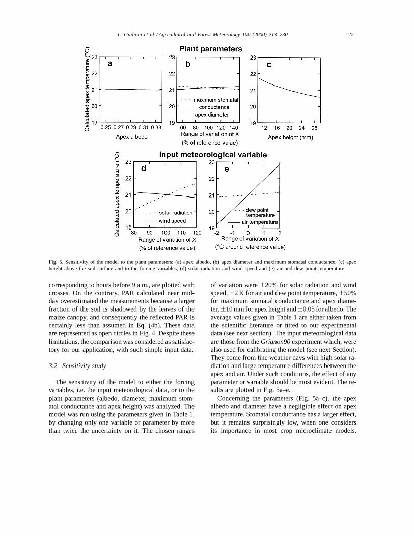
Fig. 5. Sensitivity of the model to the plant parameters: (a) apex albedo, (b) apex diameter and maximum stomatal conductance, (c) apexheight above the soil surface and to the forcing variables, (d) solar radiation and wind speed and (e) air and dew point temperature.

corresponding to hours before 9 a.m., are plotted withcrosses. On the contrary, PAR calculated near mid-day overestimated the measurements because a largerfraction of the soil is shadowed by the leaves of themaize canopy, and consequently the reflected PAR iscertainly less than assumed in Eq. (4b). These dataare represented as open circles in Fig. 4. Despite theselimitations, the comparison was considered as satisfac-tory for our application, with such simple input data.

3.2. Sensitivity study

The sensitivity of the model to either the forcingvariables, i.e. the input meteorological data, or to theplant parameters (albedo, diameter, maximum stom-atal conductance and apex height) was analyzed. Themodel was run using the parameters given in Table 1,by changing only one variable or parameter by morethan twice the uncertainty on it. The chosen ranges

of variation were±20% for solar radiation and windspeed,±2 K for air and dew point temperature,±50%for maximum stomatal conductance and apex diame-ter,±10 mm for apex height and±0.05 for albedo. Theaverage values given in Table 1 are either taken fromthe scientific literature or fitted to our experimentaldata (see next section). The input meteorological dataare those from theGrignon90experiment which, werealso used for calibrating the model (see next Section).They come from fine weather days with high solar ra-diation and large temperature differences between theapex and air. Under such conditions, the effect of anyparameter or variable should be most evident. The re-sults are plotted in Fig. 5a–e.

Concerning the parameters (Fig. 5a–c), the apexalbedo and diameter have a negligible effect on apextemperature. Stomatal conductance has a larger effect,but it remains surprisingly low, when one considersits importance in most crop microclimate models.

222 L. Guilioni et al. / Agricultural and Forest Meteorology 100 (2000) 213–230

Finally, the only plant parameter to which the modelis sensitive, is the apex height. This is the conse-quence of the steep air temperature variation withheight near the soil surface.

For the meteorological variables (Fig. 5d–e), thesensitivity is larger. It remains low for the dew pointtemperature. It is slightly larger for wind speed. Thesensitivity to solar radiation is large (±0.8 K for achange in solar radiation of 20%), but the calculatedapex temperature is most sensitive to the air tempera-ture (±1.8 K for a change in air temperature of±2 K).

3.3. Model calibration

The sources of uncertainty in this model can beclassified as relative to either the local energy balanceof the apex, or to the way of estimating the micro-climatic variables at apex height. Most parameters inthe local energy balance could be directly determined(size, soil albedo), or chosen from the literature (apexalbedo, emissivity, maximum stomatal conductance)(Table 1). Moreover, the sensitivity study showed thatthe calculated apex temperature was not very sensi-tive to these parameters, but was very sensitive to airtemperature.

Consequently, the air temperature at apex heightmust be determined as precisely as possible. For this,the main parameter to know is the roughness length(Eq. (2)). However, it is not possible to use an aero-dynamic roughness length directly estimated from thephysical characteristics of the soil surface and themaize crop, using simple relations with the physi-cal surface roughness (height of obstacles;. . . ) fortwo reasons. First, the logarithmic wind and temper-ature profiles cannot be extended down to the apexheight, because the flux-gradient relationships are notstrictly valid at lowz/zo ratios (Tennekes, 1973; Cel-lier and Brunet, 1992). Secondly, it is not straight-forward to derive one roughness height for the wholewind and temperature profile from the reference heightto the soil surface, when two flows should be con-sidered: one above the canopy and another near thesoil surface (the maize crop was generally taller than0.3–0.4 m when the LAI reached 0.5). Thus, as it couldnot be determined a priori, the roughness length wasused as a fitting parameter for the model. For the rea-sons expressed above, it could not be considered as

Fig. 6. Roughness length dependence of the average and of thestandard deviation of the absolute value of the difference betweencalculated and measured apex temperatures. The input data arethose from theGrignon90experiment.

a realistic roughness length but only as a way to re-late air temperature at apex height to air temperatureat screen height. Classical flux-gradient relationships(Eqs. (2)–(3)) were used in order to account for the in-fluence of the surface energy balance and the turbulentflow characteristics on the temperature profile. Usingthe Grignon90experiment, the roughness length giv-ing the best fit between calculated and observed apextemperatures was determined. The observed temper-ature was taken as the average of the six apex tem-peratures measured in this experiment. In Fig. 6 areplotted the average and the standard deviation of theabsolute value of the difference between calculatedand measured apex temperatures. Both curves showan optimum for roughness lengths between 0.2 and0.6 mm, with a minimum value at 0.3 mm. Thus, aroughness length of 0.3 mm was chosen. It is muchless than the roughness length that could have beendetermined from the crop height and leaf area den-sity, i.e. 10–40 mm. This confirms that this roughnesslength is nothing more than a fitting parameter.

On Fig. 7 are presented the observed and calculatedapex temperatures during theGrignon90experiment(with zo = 0.3 mm). It can be seen that the model givesa fair estimate of the actual apex temperature at anytime in the day, with no drift during the experimentalperiod. The maximum during the day and the responseto changes in solar radiation are well simulated. This

L. Guilioni et al. / Agricultural and Forest Meteorology 100 (2000) 213–230 223

Fig. 7. Air temperature, measured and calculated apex temperatureduring theGrignon90experiment.

is important because it is during fine weather days thatthe temperature difference between apex and air is atits largest. The gradual temperature decrease in thenight and the minimum are also well simulated, eventhough the energy transfer processes are very differentduring day and night.

3.4. Model validation with other datasets

The model with the roughness length determinedover theGrignon90experiment has been applied to theother independent datasets presented previously. Thiscomparison was made only on the daytime period,between sunrise and sunset, because this is the pe-riod when the temperature differences are the largest.Moreover, it is often biased to compare averages cal-culated over a 24 h period, because the energy transferprocesses are opposite between day and night. Thus,a bad account of energy transfers could give the sameaverage, while the temperature may be underestimatedduring day and overestimated during night, or the re-verse. The results are given in Fig. 8 and Table 2. Theaverages and dispersion are larger on these experi-

Table 2Average and standard deviation (K) of the difference between observed and calculated apex temperature during the day (Rs ≥ 50 W m−2)

Experiment Grignon90 Grignon93A Grignon93B Brosses Lacour

Number of values 168 389 299 161 161Average 0.20 0.06 −0.50 −0.30 0.64Standard deviation 0.69 1.27 1.17 1.36 1.93

Fig. 8. Comparison of half hourly values of calculated andmeasured temperature difference between the apex and air atscreen level, for (a)Lacour, (b) Brosses, (c) Grignon93Aand (d)Grignon93Bexperiments.

ments than onGrignon90. This is, of course, partly be-cause the model was calibrated withGrignon90data,but also because the weather was much more chang-ing over these experiments, with frequent rainfall andchanges in solar radiation, which induced a great vari-ability in air and soil surface temperatures.

4. Discussion

The experimental results showed that the apex tem-perature was very different from air temperature mea-sured at screen height. This is mainly because, duringthe early growth stages, i.e. the first weeks after sow-ing, the apex is near the soil surface, which is muchwarmer than the air at 2 m. During theGrignon90ex-periment, the temperature difference between the soilsurface and air at screen height was more than 15–20 Kevery day near midday. For a given air temperature,the apex temperature can be similar to air tempera-ture at screen height in the case of a cloudy day, or

224 L. Guilioni et al. / Agricultural and Forest Meteorology 100 (2000) 213–230

be 5–10 K warmer during day and 2–3 K lower duringnight in the case of a cloudless day. Therefore, the re-lation between apex temperature and air temperaturein a meteorological station is not straightforward. Itmay be different both for average and extreme tem-peratures. This difference should be considered whenanalyzing the response of a maize crop to either hightemperatures — which may diminish photosynthesis— or low temperatures (frost). Due to the asymmetryof the temperature difference, the daily average (over24 h) of apex temperature is larger than that of airtemperature. The difference ranged from 0 to 2 K onour experimental datasets. Such differences may havestrong implications for accounting for the effects oftemperature on growth and development.

The model that is presented in this paper should al-low replacement of air temperature by an apex tem-perature in crop models, or for estimating the riskof climatic stress (frost, heat stress). It is particularlyadapted for operational application since (1) it usesonly standard meteorological data and (2) some impre-cision in the plant parameters is permitted, because thesensitivity study showed that the model was insensi-tive to the plant parameters. The good agreement afterfitting between calculated and measured apex temper-ature at any time in the day on theGrignon90datasetshowed that the energy balance approach was welladapted to this application. The model behaved fairlywell under both daytime and night-time conditions,which are very different from an energy balance pointof view: stable atmospheric conditions, no evaporationand a radiation deficit occur during the night, whiledaytime is characterized by a high radiation input,evaporation regulated by stomata, larger wind speed,and very large soil surface temperatures. In particular,the fair agreement between calculated and measuredapex temperature near sunset and sunrise, when tem-perature changes rapidly, shows that the hypothesis ofstationarity of the energy balance over the consideredtime step (30 min) was reasonable. This allows one toestimate with a good accuracy the average, minimum,and maximum temperatures.

Such a model also helps in interpreting apex tem-perature and factors that determine it. A surprisingresult was the low sensitivity of the model to stomatalconductance. This is mainly because evaporation is aminor term of the energy balance in the case of a maizeapex. In fact, due to shading by leaves, and to the low

transmittance of the leaves for PAR, the stomatal con-ductance was low and the evaporation, too. The tem-perature is then mainly determined by an equilibriumbetween net radiation,Rnm, and sensible heat flux,Hm, which is large for small temperature differences.Over theGrignon90dataset, the calculated sensibleheat flux was approximately proportional to thecalculated temperature difference between theapex and the air at apex height, with a slope of220 W m−2 K−1. Net radiation was always less than250 W m−2. An uncertainty of±50% on apex tran-spiration — which would result in a flux error ofapproximately 50 W m−2 as calculated by the modelon theGrignon90data — would be compensated bya variation in Hm with a change of 0.2 K in apextemperature. Another result of the sensitivity study,was the relatively low response of apex temperatureto solar radiation (0.8 K for a change in solar ra-diation of ±20%). This may also be explained bythe high aerodynamic conductance of the apex, butalso by the change in stomatal conductance. ThePAR radiation reaching the apex was always low(<500mmol m−2 s−1), a level where stomatal conduc-tance is still increasing with increasing PAR (see Fig.3). Thus, any increase in solar radiation was partlycompensated by an increase in evaporation, whichmakes the apex temperature generally close to the airtemperature at the same height. The calculated tem-perature differences between the apex and air at thesame height on theGrignon90 dataset were alwaysless than 0.8 K, whereas the temperature differencebetween the air at the apex height (2 cm above soilsurface) and air at the reference height (2 m) oftenreached 6 K near midday.

Finally, it can be concluded that the lack of knowl-edge about the energy exchange parameters of a maizeapex is not a great problem for estimating apex temper-ature because it is not very sensitive to most plant pa-rameters. This is mainly because (i) the apex receivesa low amount of radiation due to the overlying leavesprotecting it from direct solar radiation, (ii) a sig-nificant fraction of this radiative energy is consumedby evaporation, which transforms energy at constanttemperature and (iii) the small aerodynamic resistancemakes the sensible heat flux increase rapidly when theapex temperature goes above air temperature.

Due to this small temperature difference betweenthe air and the apex, it could be argued that the apex

L. Guilioni et al. / Agricultural and Forest Meteorology 100 (2000) 213–230 225

energy balance module is not strictly necessary to esti-mate apex temperature under such conditions. In orderto check this, the model was run in a simplified ver-sion by considering that apex temperature was equalto air temperature at the same height. The model thenonly consisted in the soil surface energy balance pre-sented in Appendix A. As previously done for thecomplete model the surface roughness length was fit-ted on theGrignon90dataset. The best value is close tothe previous one: 0.35 mm instead of 0.30 mm. How-ever, both the absolute error and the residual stan-dard deviation are larger by approximately 0.1 K, i.e.10–15 and 15–20%, respectively, with this simplermodel compared with the initial model. Using a rough-ness length based on the canopy physical description,i.e. values comprised between 10 and 40 mm leadsto much worse results. Both the absolute error andthe residual standard deviation are multiplied by morethan 2. Moreover, it must be emphasized that usingonly the soil surface energy balance model producesa simplification only by reducing the number of equa-tions. The input meteorological variables, which arethe key-point for deciding whether a model is opera-tional or not, are the same for both models. The com-plete model has the advantage of being more generaland easily adaptable for calculating the range of apextemperature (i.e. shaded and sunlit apex) or the tem-perature of any plant organ. For example, for an or-gan placed near the top of the crop (leaf, flower, ear),the solar radiation absorption and the stomatal con-ductance would be much more relevant to estimate theorgan temperature because the organ is directly ex-posed to the solar radiation. Moreover, the differencebetween the temperature of the air at screen heightand the temperature of the air surrounding the organshould be less, because the organ is higher above thesoil surface.

Thus, modeling the temperature of a vegetation or-gan needs accurate modeling of the microclimate nearthe considered organ. In this case, one must determineprecisely the wind speed and air temperature at apexheight from the standard values taken at a referenceheight. The soil surface temperature must be deter-mined accurately under all conditions: during nightand day, with low or large solar radiation or windspeed, with a wet or dry soil. It requires an accountto be taken of the soil properties, because they influ-ence greatly the soil surface energy balance. This is

what makes the model difficult to apply under differ-ent conditions. This is certainly the main reason whythe model results were not so good in 1993 in Grignon,or for the Lacour or Brossesexperiments. The soilsconditions were very different, with a chalky (Brosses)and a sandy soil (Lacour) compared with a clay loamsoil (Grignon). The meteorological conditions werealso very different, with frequent rain. In such condi-tions, soil evaporation must be simulated well in or-der to estimate soil surface temperature. Despite theseconstraints, the results remained satisfactory when themodel was applied under very different conditions,with no systematic deviation and a standard deviationwhich is less than twice that of the calibration experi-ment (Grignon90). This means that the calibrating fac-tor, the roughness length, can be considered as robustenough to make the model applicable to different sites.We obtained the least satisfactory results in theLa-cour experiment. This might be because the soil wasmuch more sandy, but more likely because this fieldwas irrigated. Irrigation caused very rapid changes intemperatures, and wetted the apex, which created in-consistent datasets, with a wet apex at the same timeas the solar radiation was large. This case is criticalbecause the model does not account for water inter-ception by the apex. Under a natural climate, the apexis only wet when it rains, and, in this case, its tem-perature cannot be much higher than air temperaturedue to low solar radiation in addition to wetness andlarge soil evaporation. When solar radiation is largeand the apex is wet, its temperature cannot be muchlarger than air temperature as expected, because of alarge energy consumption by evaporation. Thus, ne-glecting water interception is not critical in the modelunder most conditions, unless the crop is irrigated.

5. Concluding remarks

This model is able to estimate with a fair accuracythe temperature difference between air at screen heightand the apex, which is close to the soil surface for sev-eral weeks after emergence. This model was able toprovide good estimates of apex temperature under verydifferent meteorological and soil conditions, includingsoil type and soil wetness. It gave a good descriptionof apex temperature change with time at hourly timesteps, and could consequently give the minimum and

226 L. Guilioni et al. / Agricultural and Forest Meteorology 100 (2000) 213–230

maximum temperatures, which are often the relevanttemperatures to explain variations in growth and devel-opment (Weaich et al., 1996). Owing to its mechanisticapproach, this model could be adapted to estimatingthe temperature of very different types of plant organs,such as flowers, ears or individual leaves. However,the calibration on the roughness length, which provedto be robust, should be made again when using themodel over a different vegetation organ.

The most important part of this model is the esti-mation of the forcing variables near the apex: apexradiation balance, wind speed, air humidity and, mostimportantly, air temperature at apex height. This ismade especially complex, due to the proximity of thesoil surface where strong temperature and wind speedgradients are likely to occur. Estimating apex temper-ature accurately required a good estimate of soil sur-face temperature using also easily available input data.One practical result of this study was to show that apextemperature could be almost directly derived from airtemperature at apex height. This is evidenced froman analysis of the different terms of the apex energybalance estimated with the model: apex net radiationis low due to shadowing by overlying leaves and lowaerodynamic resistance prevents the apex temperaturefrom increasing by more than 1◦C or so above air tem-perature at apex height. However, using the apex en-ergy balance gives a slightly better apex temperatureestimate, while not requiring more input variables.

Symbol Significance Equation Unit

am apex albedo Eq. (4a) dimensionlessas soil albedo Eqs. (4b), (4c) and (B.2) dimensionlessasd soil albedo under dry conditions Eq. (B.3) dimensionlessasw soil albedo under wet conditions Eq. (B.3) dimensionlesscp air specific heat at constant pressure (cp = 1005) Eqs. (7) and (9) J kg−1 K−1

D water vapor pressure deficit Eq. (10) hPadm apex diameter Eq. (8) me atmospheric vapor pressure Eq. (9) hPaEm apex evaporation Eqs. (1) and (9) W m−2

Es soil evaporation Eqs. (B.1) and (B.9) W m−2

Gm apex energy storage Eq. (1) W m−2

Gs soil heat flux Eqs. (B.1) and (B.7) W m−2

g gravity acceleration (g= 9.81) m s−2

gm apex aerodynamic conductance Eqs. (7) and (8) m s−1

gs apex stomatal conductance Eqs. (9) and (10) m s−1

gsm minimum stomatal conductance Eq. (10) m s−1

One important constraint when setting up the modelwas to use only data collected at a meteorologicalstation. This made it difficult to estimate the forcingvariables at apex height in order to solve the apexenergy balance. However, this makes it possible tointegrate the present model into crop models, inorder to account better for the effect of tempera-ture on growth and development. However, mosttemperature-dependent laws and thresholds for ther-mal time are determined using air temperature. Useof modeled apex temperature in crop models wouldrequire modification of the parameters relating cropgrowth and development to temperature. This couldcertainly be done with previously collected datasets,complemented by the meteorological data requiredby our model.

Acknowledgements

We thank B. Andrieu and J.-F. Castell for fruitfuldiscussion and help in experiments. We are also in-debted to B. Durand for collecting and processing theGrignon93data. The reviewers and the editor are alsoacknowledged for helpful comments on the model.

Appendix A

Notations

L. Guilioni et al. / Agricultural and Forest Meteorology 100 (2000) 213–230 227

Symbol Significance Equation Unit

gsM maximum stomatal conductance Eq. (10) m s−1

gv thermal diffusion conductance Eq. (9) m s−1

h relative humidity at soil surface Eqs. (B.9) and (B.10) dimensionlessHm apex sensible heat flux Eqs. (1) and (7) W m−2

Hs atmospheric sensible heat flux Eqs. (B.1) and (B.8) W m−2

k von Karman constant (k= 0.40) Eqs. (2) and (3) dimensionlessKD coefficient of Eq. (10) Eq. (10) hPaKPAR coefficient of Eq. (10) Eq. (10) mmol m−2 s−1

L Monin–Obukhov length Eqs. (2) and (3) mQPAR PAR at apex height Eq. (10) mmol m−2 s−1

ra soil surface aerodynamic resistance Eq. (B.8) s m−1

Ra atmospheric long-wave radiation Eq. (B.2) W m−2

Ram apex ‘atmospheric’ radiation Eqs. (5) and (6) W m−2

RLWm apex long-wave radiation balance Eq. (5) W m−2

RNIR incident NIR above the crop Eqs. (4c) and (4e) W m−2

RNIRm NIR at the apex surface Eqs. (4a) and (4c) W m−2

Rnm apex net radiation Eq. (1) W m−2

Rns soil surface net radiation Eqs. (B.1) and (B.2) W m−2

RPAR incident PAR above the crop Eqs. (4b), (4d) and (4e) W m−2

RPARm PAR at the apex surface Eqs. (4a) and (4b) W m−2

Rs solar radiation Eqs. (4d), (4e) and (B.2) W m−2

RSWm apex short-wave radiation balance Eq. (4a) W m−2

rv apex aerodynamic resistance for evaporation Eq. (9) s m−1

T(z) air temperature at heightz Eq. (3) K or ◦CTa air temperature at screen height Eqs. (6), (B.4) and (B.8) K or◦CTam air temperature at apex height Eq. (7) K or◦CTm apex temperature Eqs. (5) and (7) K or◦CTs soil surface temperature Eqs. (6), (B.2), (B.8) and (B.9) K or◦CT∗ scale temperature for air temperature profile Eq. (3) K or◦Cu(z) wind speed at heightz Eq. (2) m s−1

U wind speed at the meteorological station Eq. (B.7) m s−1

Um wind speed at apex height Eq. (8) m s−1

u∗ friction velocity Eq. (2) m s−1

wFC soil water content at field capacity Eq. (B.10) m3 m−3

wg soil surface water content Eq. (B.10) m3 m−3

wwilt soil water content at wilting point Eq. (B.3) m3 m−3

z height above soil surface Eqs. (2) and (3) mzm height of the apex above the soil surface mzo roughness height for wind speed profile Eq. (2) mzoh roughness height for temperature profile Eq. (3) mα fraction of PAR in solar radiation Eq. (4d) dimensionlessεa atmospheric emissivity Eqs. (B.4) and (B.5) dimensionlessεaB clear sky atmospheric emissivity Eqs. (B.5) and (B.6) dimensionlessεm apex emissivity Eq. (5) dimensionlessεs soil emissivity Eq. (B.2) dimensionlessϕGH phase shift function in Eq. (B.7) Eq. (B.7) dimensionlessγ psychrometric constant (γ = 66) Eqs. (9) and (B.9) Pa K−1

λ latent heat of vaporization Eqs. (1), (9) and (B.9) J kg−1

ρ air density Eqs. (7), (9), (B.8) and (B.9) kg m−3

σ Stefan Boltzman constant (σ = 5.67× 10−8) Eqs. (5), (6), (B.2) and (B.4) W m−2 K−4

τNIR leaf transmissivity for near infrared radiation Eq. (4c) dimensionlessτPAR leaf transmissivity for PAR Eq. (4b) dimensionless9H stability function for temperature profile Eq. (3) dimensionless9M stability function for wind speed profile Eq. (2) dimensionless

228 L. Guilioni et al. / Agricultural and Forest Meteorology 100 (2000) 213–230

Appendix B. Soil surface temperature calculation

Soil surface temperature can be calculated from anenergy balance of the soil surface,

Rns − Gs = Hs + λEs (B.1)

whereRns is the net radiation,Gs is soil heat flux byconduction,Hs is the sensible heat flux to the atmo-sphere, andλEs is soil evaporation. All fluxes are ex-pressed in W m−2. They have to be parameterized us-ing only standard meteorological data and easily avail-able soil parameters.

Net radiation can be expressed as follows:

Rns = (1 − as)Rs + εs(Ra − σT 4s ) (B.2)

For the sake of simplicity, the soil emissivity,εs, wastaken equal to 1. The variation of soil albedo from dryto wet conditions was accounted for by the followingsinusoidal function of soil surface water content, fromNoilhan and Planton (1989):

as = asd − 0.5

{1 − cos

[π(wg − wwilt )

wFC − wwilt

]}

×(asd − asw) (B.3)

The atmospheric long-wave radiation,Ra, was con-sidered as constant throughout the day, and it was cal-culated from daily averages of air temperature and hu-midity, following Brutsaert (1975, 1982).

Ra = εaσT 4s (B.4)

with

εa = εaB + n(1 − εaB)

(1 − 4 × 11

T

)(B.5)

and

εaB = 1.24( e

T

)1/7(B.6)

The cloudiness,n, can be estimated from the ratioof measured solar radiation to the extra-terrestrialradiation, calculated from astronomical formulas(Unsworth and Monteith, 1985; Spitters et al., 1985).

The soil heat flux,G, was estimated from its ratioto H with a simple unique function of wind speed,U,for all soil conditions, including a phase shift,ϕGH,between these two fluxes (Cellier et al., 1996):

Gs

Hs= ϕGH

1.36

U1/2(B.7)

The sensible heat flux,Hs, is proportional to theair temperature difference between heightzoh, To, andscreen height.To is assumed to be equal to the surfacetemperature. The proportionality coefficient,ra, is ex-pressed in a resistance form that includes stability cor-rections according to the theory of turbulent transferin the surface boundary layer (Brutsaert, 1982).

Hs = ρcpTs − Ta

ra(B.8)

Soil evaporation is parameterized in a similar form,using the difference in air humidity

λEs = ρcp

γ

hP (Ts) − P(Td)

ra(B.9)

whereP(T) is the saturation vapor pressure at tem-peratureT, andh is the relative humidity in the topsoil layer calculated as follows (Noilhan and Planton,1989):

h = 0.5

[1 − cos

(πwg

wFC

)](B.10)

where wg is the top soil water content, andwFC issoil water content at field capacity. Calculatingwg wasmade by using a simplified water balance in the topsoil layer. The model proposed by Noilhan and Planton(1989) was used. The only required input data is thesoil texture. The different soil hydraulic parametersare derived from the texture by a classification into 11soil classes proposed by Clapp and Hornberger (1978).Following Toya and Yasuda (1988) and Noilhan andPlanton (1989), the depth of the soil top layer wastaken equal to 50 mm.

Eqs. (B.1)–(B.10) were solved at each time step ofthe model (i.e. 30 min) using an iterative procedure,and the surface temperature and air surface humid-ity were then used to calculate air temperature andhumidity at apex height.

References

Aston, A.R., 1987. Apex and root temperature and the early growthof wheat. Aust. J. Agric. Res. 38, 231–238.

Beauchamp, E.G., Lathwell, D.J., 1966. Root-zone temperatureeffects on the early development of maize. Plant Soil 26, 224–234.

Beauchamp, E.G., Torrance, J.K., 1969. Temperature gradientswithin young maize plant stalks as influenced by aerial androot zone temperature. Plant Soil 2, 241–251.

L. Guilioni et al. / Agricultural and Forest Meteorology 100 (2000) 213–230 229

Ben Haj Salah, H., Tardieu, F., 1996. Quantitative analysisof the combined effects of temperature, evaporative demandand light on leaf elongation rate in well-watered field andlaboratory-grown maize plants. J. Exp. Bot. 47, 1689–1698.

Bethenod, O., Tardieu, F., 1990. Water use efficiency in field-grownmaize. Effect of soil structure. In: Balltscheffsky, M. (Ed.),Current Research in Photosynthesis, vol. 4, Kluwer AcademicPublishers, Dordrecht, pp. 737–740.

Bollero, G.A., Bullock, D.G., Hollinger, S.E., 1996. Soiltemperature and planting date effects on corn yield, leaf areaand plant development. Agron. J. 88, 385–390.

Brouwer, R., Kleinendorst, A., Locher, J.T., 1970. Growth responseof maize plants to temperature. In: Plant Response to ClimaticFactors, UNESCO, pp. 169–174.

Brutsaert, W., 1975. On a derivable formula for long-wave radiationfrom clear skies. Water Resour. Res. 11, 742–744.

Brutsaert, W., 1982. Evaporation into the Atmosphere, Reidel,Dordrecht, Netherlands, 229 pp.

Cellier, P., Brunet, Y., 1992. Flux-gradient relationships above tallplant canopies. Agric. For. Meteorol. 58, 93–117.

Cellier, P., Ruget, F., Chartier, M., Bonhomme, R., 1993.Estimating the temperature of a maize apex during the earlygrowth stages. Agric. For. Meteorol. 63, 35–54.

Cellier, P., Richard, G., Robin, P., 1996. Partition of sensible heatfluxes into bare soil and the atmosphere. Agric. For. Meteorol.82, 245–265.

Chartier, M., Bonchrétien, P., Allirand, J.M., Gosse, G., 1989.Utilisation de cellules au silicium amorphe pour la mesuredu rayonnement photosynthétiquement actif (400–700 nm).Agronomie 9, 281–284.

Clapp, R.B., Hornberger, G.M., 1978. Empirical equations for somesoil hydraulic properties. Water Resour. Res. 14, 601–604.

Davies, J.A., Buttimor, P.H., 1969. Reflection coefficients, heatingcoefficients and net radiation at Simcoe. S. Ont. Agric.Meteorol. 6, 673–686.

De Reaumur, R.A., 1735. Observations du thermomètre faites àParis pendant l’année MDCCXXXV comparées à celles qui ontété faites sous la ligne à l’Isle-de-France, à Alger et en quelquesunes de nos Isles de l’Amérique, Mémoires de l’Acad.Roy-desSci., pp. 545–576.

Duburcq, J.B., Bonhomme, R., Derieux, M., 1983. Durée desphases végétative et reproductrice chez le maıs. Influence dugénotype et du milieu. Agronomie 3, 941–946.

Durand, R., Bonhomme, R., Derieux, M., 1982. Seuil optimal dessommes de températures. Application au maıs (Zea mays L.).Agronomie 2, 589–597.

Dyer, A.J., Hicks, B.B., 1970. Flux-gradient relationships in theconstant flux layer. Quart. J. R. Meteorol. Soc. 96, 715–721.

Finnigan, J.J., Raupach, M.R., 1987. Transfer processes in plantcanopies in relation to stomatal characteristics. In: Zeiger, E.,Farquhar, G.D., Cowan, I.R. (Eds.), Stomatal Function, StanfordUniversity Press, Stanford, pp. 385–429.

Gallagher, J.N., 1979. Field studies of Cereal Leaf Growth. I.Initiation and expansion in relation to temperature and ontogeny.J. Exp. Bot. 30, 625–636.

Jamieson, P.D., Brooking, I.R., Porter, J.R., Wilson, D.R.,1995. Prediction of leaf appearance in wheat: a question oftemperature. Field Crop Res. 41, 35–44.

Jarvis, P.G., 1976. The interpretation of the variations in leaf waterpotential and stomatal conductance found in canopies in thefield. Philos. Trans. R. Soc. Lond. Ser. B. 273, 593–610.

Jones, H.G., 1992. Plants and microclimate. In: A QuantitativeApproach to Environmental Plant Physiology, 2nd ed.,Cambridge University Press, New York, pp. 131–161.

Kleinendorst, A., Brouwer, R., 1970. The effect of temperatureof the root medium and of the growing point of the shoot ongrowth water content and sugar content of maize leaves. Neth.J. Agric. Sci. 18, 140–148.

Noilhan, J., Planton, S., 1989. A simple parameterization of landsurface processes for meteorological models. Monthly WeatherRev. 117, 536–549.

Olioso, A., Bethenod, O., Rambal, S., Thamitchian, M., 1995.Comparison of empirical leaf photosynthesis and stomatalconductance models. In: 10th International PhotosynthesisCongress, Montpellier (FRA), 20–25 August 1995, 4 pp.

Ong, C.K., 1983. Response to temperature in a stand of PearlMillet (Pennisetum typhoides S. & H.) Vegetative development.J. Exp. Bot. 34, 322–336.

Paulson, C.A., 1970. The mathematical representation of windspeed and temperature profiles in the unstable surface layer. J.Appl. Meteorol. 9, 857–861.

Peacock, J.M., 1975. Temperature and leaf growth in Loliumperenne. II. The site of temperature perception. J. Appl. Ecol.12, 115–123.

Ritchie, J.T., NeSmith, D.S., 1991. Temperature and cropdevelopment. In: Hanks, J., Ritchie, J.T. (Eds.), Modeling Plantand Soil Systems, ASA Spec. Publi 31. ASA, CSSA, SSSA,Madison, pp. 5–29.

Schoch, P.G., Silvy, A., 1978. Méthode simple de numérationdes stomates et des cellules de l’épiderme des végétaux. Ann.Amélior. Plantes 28, 455–461.

Sharratt, B.S., 1991. Shoot growth root length density and wateruse of barley grown at different soil temperature. Agron. J. 83,237–239.

Spitters, C.J.T., Toussaint, H.A.J.M., Goudriaan, J., 1985.Separating the diffuse and direct components of global radiationand its implications for modeling canopy photosynthesis. PartI. Components of incoming radiation. Agric. For. Meteorol. 38,217–229.

Swan, J.B., Schneider, E.C., Moncrief, J.F., Paulson, W.H.,Peterson, A.E., 1987. Estimating corn growth, and grainmoisture from air growing degree days and residue cover.Agron. J. 79, 53–60.

Tennekes, H., 1973. The logarithmic wind profile. J. Atmos. Sci.30, 234–238.

Toya, T., Yasuda, N., 1988. Parameterization of evaporation froma non-saturated surface for application in numerical predictionmodels. J. Meteorol. Soc. Japan 66, 729–739.

Turner, N.C., 1991. Measurement and influence of environmentalplant factors on stomatal conductance in the field. Agric. For.Meteorol. 54, 137–154.

Unsworth, M.H., Monteith, J.L., 1985. Long wave radiation at theground. I. Angular distribution of incoming radiation. Quart. J.R. Meteorol. Soc. 101, 13–24.

230 L. Guilioni et al. / Agricultural and Forest Meteorology 100 (2000) 213–230

Warrington, I.J., Kanemasu, E.T., 1983. Corn growth responseto temperature and photoperiod. II. Leaf initiation and leafappearance rates. Agron. J. 75, 755–761.

Watts, W.R., 1972a. Leaf extension in Zea mays. I. Leaf extensionand water potential in relation to root-zone and air temperatures.J. Exp. Bot. 76, 704–712.

Watts, W.R., 1972b. Leaf extension in Zea mays. II. Leaf extensionin response to independent variation of the apical meristem, of

the air around the leaves, and of the root-zone. J. Exp. Bot.76, 713–721.

Weaich, K., Bristow, K.L., Cass, A., 1996. Modeling preemergentmaize shoot growth. II High temperature stress conditions.Agron. J. 88, 398–403.

Weiss, A., Norman, J.M., 1985. Partioning solar radiation intodirect and diffuse visible and near-infrared components. Agric.For. Meteorol. 34, 205–213.