A MODEL FOR THE CALCULATION OF CO2 EMISSIONS ...

Proceedings of the 1st Iberic Conference on Theoretical and Experimental Mechanics and Materials /

11th National Congress on Experimental Mechanics. Porto/Portugal 4-7 November 2018.

Ed. J.F. Silva Gomes. INEGI/FEUP (2018); ISBN: 978-989-20-8771-9; pp. 397-418.

-397-

PAPER REF: 7430

A MODEL FOR THE CALCULATION OF CO2 EMISSIONS AND FUEL

CONSUMPTION OF A DIESEL ENGINE DRIVEN CAR IN THE NEDC

Pedro de F. V. Carvalheira(*)

Departamento de Engenharia Mecânica, Faculdade de Ciências e Tecnologia da Universidade de Coimbra

Coimbra, Portugal (*)

Email: [email protected]

ABSTRACT

This work describes a model developed to predict the CO2 emissions and fuel consumption of

a passenger car driven by a Diesel engine in the New European Driving Cycle (NEDC). The

NEDC is a normalized driving cycle established by the European Community (EC) to make

measurements of pollutant emissions and fuel consumption of car vehicles to be homologated

for the European market. To validate the model the results of a computer program that

incorporates this model and vehicle data for a Volkswagen Jetta 2.0 TDI of 2009 are

compared with the results published by the vehicle manufacturer. Then the model is used to

study the effect of some vehicle design variables on the CO2 emissions and fuel consumption

reduction and the results of this study are presented.

Keywords: NEDC modelling, CO2 emissions, fuel consumption, VW Jetta 2.0 TDI.

1. INTRODUCTION

The NEDC cycle is constituted by two parts. Part one is the urban driving cycle (UDC) and

part two is the extra-urban diving cycle (EUDC). The UDC is constituted by four elementary

ECE-15 urban driving cycles (Directive 70/220/EEC). Each elementary urban driving cycle

has duration of 195 s, the total distance displaced is 1.013 km, the maximum speed is 50 km/h

and the average speed of the cycle is 18.70 km/h. The EUDC has duration of 400 s, the total

distance displaced is 6.955 km, the maximum speed is 120 km/h and the average speed of the

cycle is 62.60 km/h. The NEDC has duration of 1180 s, the total distance displaced is 11.007

km, the maximum speed is 120 km/h and the average speed of the cycle is 33.58 km/h

(Directive 91/441/EEC). The NEDC test is performed in a chassis dynamometer equipped

with means of load and inertia simulation. The chassis dynamometer can be fit with different

disks with inertia of rotation equivalent to the inertia of translation of the mass of the vehicle

and can produce a variable load with the vehicle speed to simulate the rolling resistance and

the aerodynamic drag force in the vehicle. The CO2 emissions and fuel consumption depend

on the ambient conditions during the test, on the operating variables of the vehicle and on

some design characteristics of the vehicle. The ambient conditions during the test and the

operating variables of the vehicle are specified in ECE Regulation ECE-R-83/05. Among the

design variables of the vehicle that have more influence on the CO2 emissions and fuel

consumption are the vehicle mass, the vehicle coefficient of rolling resistance, the vehicle

drag coefficient and frontal area, the transmission system gear ratios and efficiency, the

engine brake specific fuel consumption as a function of engine speed and brake torque, the

Track-B: Computational Mechanics

-398-

moment of inertia of rotation relative to their rotation axis of the wheels, of the components of

the transmission system and of the engine.

2. THE NEW EUROPEAN DRIVING CYCLE

The NEDC cycle is constituted by two parts. Part one is the urban driving cycle (UDC) and

part two is the extra-urban driving cycle (EUDC). The UDC is constituted by four elementary

ECE-15 urban driving cycles (Directive 70/220/EEC). The elementary urban driving cycle

ECE-15 is constituted by 25 operations and is presented in Directive 70/220/EEC or in

Directive 91/441/EEC. The extra-urban driving cycle is constituted by 21 operations and is

presented in Directive 91/441/EEC.

The NEDC and the test procedures are defined in the following directives and regulations,

where the most recent are updates or extensions of the preceding standards:

- Directive 70/220/EEC of 20 March 1970

- Directive 80/1268/EEC of 16 December 1980

- Directive 91/441/EEC of 26 June 1991

- Directive 93/116/EEC of 17 December 1993

- Directive 2004/3/EC of 11 February 2004

- Regulation ECE-R-83/05, Corrigendum 4 of 9 March 2007

- Regulation EC/715/2007 of 20 June 2007

- Regulation EC/443/2009 of 23 April 2009

3. NUMERICAL MODEL

3.1. DISTANCE COVERED BY THE VEHICLE

The distance covered by the vehicle is given by Eq. (1), where s is the distance covered by the

vehicle in m, v is the vehicle speed in m/s, a is the vehicle acceleration in m/s2. The subscript i

is an integer and refers to point i and the subscript i-1 refers to point i-1. In the model

developed the subscript i = 0 corresponds to t = 0 s, the subscript i = 1 corresponds to t = 0.10

s, the time step, when i increases one unit the time increases 0.10 s.

�� = �� + �� − �� + 12 �� − �� (1)

3.2. VEHICLE SPEED

The vehicle speed is given by Eq. (2).

�� = �� + �� − �� (2)

The vehicle speed in km/h, V, is given by Eq. (3) where v is the vehicle speed in m/s.

��km/h� = 3600sh km1000m × ��m/s� (3)

Proceedings TEMM2018 / CNME2018

-399-

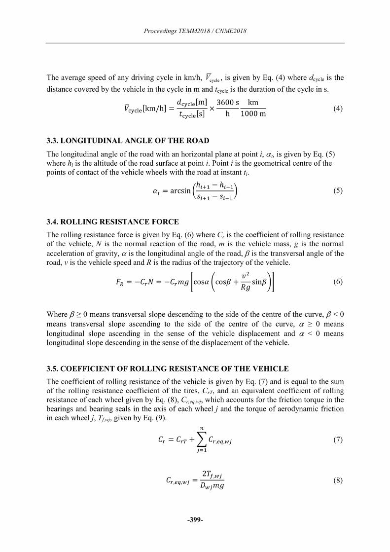
The average speed of any driving cycle in km/h, cycleV , is given by Eq. (4) where dcycle is the

distance covered by the vehicle in the cycle in m and tcycle is the duration of the cycle in s.

�� !�km/h� = "�� !�m�� !�s� × 3600sh km1000m (4)

3.3. LONGITUDINAL ANGLE OF THE ROAD

The longitudinal angle of the road with an horizontal plane at point i, αι, is given by Eq. (5)

where hi is the altitude of the road surface at point i. Point i is the geometrical centre of the

points of contact of the vehicle wheels with the road at instant ti.

#� = arcsin )ℎ�+� − ℎ��+� − �� , (5)

3.4. ROLLING RESISTANCE FORCE

The rolling resistance force is given by Eq. (6) where Cr is the coefficient of rolling resistance

of the vehicle, N is the normal reaction of the road, m is the vehicle mass, g is the normal

acceleration of gravity, α is the longitudinal angle of the road, β is the transversal angle of the

road, v is the vehicle speed and R is the radius of the trajectory of the vehicle.

-. = −/01 = −/023 4cos# 6cos7 + ��83 sin79: (6)

Where β ≥ 0 means transversal slope descending to the side of the centre of the curve, β < 0

means transversal slope ascending to the side of the centre of the curve, α ≥ 0 means

longitudinal slope ascending in the sense of the vehicle displacement and α < 0 means

longitudinal slope descending in the sense of the displacement of the vehicle.

3.5. COEFFICIENT OF ROLLING RESISTANCE OF THE VEHICLE

The coefficient of rolling resistance of the vehicle is given by Eq. (7) and is equal to the sum

of the rolling resistance coefficient of the tires, CrT, and an equivalent coefficient of rolling

resistance of each wheel given by Eq. (8), Cr,eq,wj, which accounts for the friction torque in the

bearings and bearing seals in the axis of each wheel j and the torque of aerodynamic friction

in each wheel j, Tf,wj, given by Eq. (9).

/0 = /0; + < /0,>?,@AB

AC� (7)

/0,>?,@A = 2DE,@AF@A23 (8)


-400-

DE,@A = ��,@A�� + ��,@A� + �G,@A (9)

The tire coefficient of rolling resistance depends on tire brand, model, size, inflation pressure,

tire load (Evans et al., 2009), vehicle speed, tire temperature, tire wear, surface track

roughness and type (van Brokland et al., 2009). The coefficient of rolling resistance is usually

measured with a drum and there are several standards to measure it (ISO 8767, 1992), (ISO

18164, 2005) and (ISO 28580, 2009). It can also be measured with a special mobile device to

study the influence of surface track roughness and type on the coefficient of rolling resistance

(Roovers et al., 2005), (van Brokland et al., 2009). Brokland et al. measured the coefficient of

rolling resistance of two different tires with a special mobile device in 40 different test tracks

including several types of Stone Mastic Asphalt (SMA), Dense Asphalt Concrete (DAC) 0/16,

several types of Thin Layer Asphalt, several types of Porous Asphalt Concrete (PAC), several

types of double layer Porous Asphalt Concrete (double layer PAC), several types of

rubberized surfaces, several types of surfaces dressings and with a drum according to ISO

10844. The lowest value for the coefficient of rolling resistance was obtained for SMA (0/6)

for both tires. The values of the coefficient of rolling resistance obtained for SMA (0/8), DAC

(0/16) and with a drum according to ISO 10844 where equal within experimental incertitude

for both tires. The difference between the values of the coefficient of rolling resistance for

SMA (0/6) and with a drum according to ISO 10844 is less than 0.00025.

3.6. AERODYNAMIC DRAG FORCE

The aerodynamic drag force in the vehicle in the case where there is no wind is given by Eq.

(10), where Cx is the drag friction coefficient of the vehicle, Af is the frontal area of the

vehicle, ρa is the density of air and v is the vehicle speed.

-H = −/IJE 12 KL�� (10)

Air density is given by Eq. (11) where pa is the atmospheric pressure, Ma is the molecular

weight of air, Ru is the universal gas constant and Ta is the dry-bulb air temperature.

KL = MLNL8ODL (11)

The molecular weight of air is given by Eq. (12) where airdry ~x is the mole fraction of dry air,

airdry M is the molecular weight of dry air, OH2

~x is the mole fraction of water vapor in the air,

OH2M is the molecular weight of water.

NL = PQRS�TUSNRS�TUS + PQVWXNVWX (12)

Where

NRS�TUS = 28.9641 × 10�]kg/mol


-401-

NVWX = 18.01528 × 10�]kg/mol

The mole fraction of water vapor is given by Eq. (13) where OH, 2vp is the vapor pressure of

water in the air.

PQVWX = Ma,VWXML (13)

The mole fraction of dry air is given by Eq. (14).

PQRS�TUS = 1 − PQVWX (14)

The water vapor pressure in air is given by Eq. (15) where OH, 2vsp is the saturation pressure of

water vapor in the air for the dry-bulb air temperature and φ is the relative humidity of air.

Ma,VWX = bMac,VWX (15)

The saturation pressure of water vapor is a function of air temperature and can be found in

tables of thermophysical properties of saturated water vapor or can be obtained analytically in

an approximate form by the Clausius-Clapeyron equation, Eq. (16).

Mac,VWX�DL� = Mac,VWX�D��exp 4− ℎEg,VWX�D��NVWX8O ) 1DL − 1D�,: (16)

If we consider T1 = 298.15 K Eq. (16) takes the form of Eq. (17).

Mac,VWX�DL� = 3169Pa× exp i− 2442300 Jkg × 0.01801528 kgmol8.314472J/mol ∙ K ) 1DL − 1298.15K,n

(17)

The result of Eq. (17) has an error less than 2.1 % for Ta in the range [273.15 K, 323.15 K] =

[0, 50 ºC].

3.7. DRAG FORCE COEFFICIENT

The vehicle drag force coefficient, Cx, in the general case is a function of the yaw angle of the

flow around the vehicle, β, of the angle of attack of the flow around the vehicle, α, of the

Reynolds number of the flow around the vehicle, Re, of the Mach number of the flow around

the vehicle, Ma, and of the relative roughness of the surface of the vehicle, ε/L, Eq. (18).

/I = /I o7, #, Re, Ma, rst (18)


-402-

If there is no wind the air flow around the vehicle when it moves is always aligned with the

velocity vector of the vehicle, if in addition the velocity of the vehicle coincides with the

longitudinal plane of symmetry of the vehicle the air flow around the vehicle is always

aligned with the longitudinal plane of symmetry of the vehicle and the dependence of Cx on β

disappears. If the angle of attack of the air flow around the vehicle does not changes the

dependence of Cx on α disappears. If in addition to all this air flow is low subsonic, which

means the velocity of the flow around the vehicle is much less than the speed of sound in air,

the Cx dependence on Mach number vanishes. If we consider the case that the vehicle is

hydraulically smooth, i.e. if the surface roughness of the vehicle, ε, is less than the thickness

of the linear viscous sublayer for turbulent boundary layer flows, the dependency of Cx on the

relative roughness disappears and Cx becomes only a function of the Reynolds number, Eq.

(19).

/I = /I�Re� (19)

A possible form of Eq. (19) is given by Eq. (20).

/I = /I�Re = 10u� ) Re10u,v (20)

For the case of blunt bodies most of the aerodynamic drag is due to pressure forces on the

body surface, which is the case of the external shape of the vast majority of automotive

vehicles, b = 0 or near zero and the dependency of Cx on the Reynolds number disappears or

is very low.

For the case of streamlined bodies a significant part of aerodynamic drag is due to shear

forces on the body surface that are very dependent on the Reynolds number of the flow, b ≠ 0

and the dependency of Cx on the Reynolds number is strong. For the case of the flow around

flat plates and parallel to the plates, for laminar boundary layer b = -0.50 and for turbulent

boundary layer b = -0.1428.

The Reynolds number of the flow is given by Eq. (21), where ρa is the air density, µa is the

dynamic viscosity of air, L is the total length of the vehicle and v is the velocity of the flow

around the vehicle.

Re = KL�swL (21)

The dynamic viscosity of air around the vehicle is given by Eq. (22), valid in the following

range of air temperature [250 K, 350 K] = [-23.15 ºC, 76.85 ºC].

wL�Pa ∙ s� = 1.711 × 10�x + 4.860 × 10�y × �DL�K� − 273.15� (22)

3.8. TIRE DRAG DUE TO LATERAL FORCE

The tire drag force due to the lateral force is given by Eq. (23) where FY is the lateral force

that acts in the tire and Cα is the tire cornering drag force stiffness coefficient.


-403-

-;zH = −|-||sin 6|-||/} 9 (23)

The lateral force parallel to the road is given by Eq. (24).

-| = 23 6− ��cos783 + sin79 (24)

3.9. REACTION NORMAL TO THE ROAD AND LATERAL FORCE PARALLEL

TO THE ROAD

The forces applied in a vehicle in a road with transversal slope and longitudinal slope equal to

zero in a plane normal to the velocity vector of the vehicle are the weight, the centrifugal

force, the reaction normal to the road, N, and the lateral force parallel to the road, FY. The

centrifugal force is an inertia force that is created to analyse a dynamic system as a static

system and is equal to the product of the vehicle mass by the symmetric of the centripetal

acceleration of the vehicle. Considering a system of axis whose origin is coincident with the

centre of mass of the vehicle where the yy axis is parallel to the road, oriented to the side of

the road where the altitude increases and is in a plane normal to the velocity vector of the

vehicle and where the zz axis is normal to the surface of the road and oriented from the

surface of the road to the exterior and is in a plane normal to the velocity vector of the vehicle

we can consider that in a situation of static equilibrium the sum of the forces along the yy axis

is zero, Eq. (24), and that the sum of the forces along the zz axis is zero, Eq. (25).

< -~ = 0 <=> 2 ��8 cos7 − 23sin7 + -| = 0 (25)

< -� = 0 <=> −2 ��8 sin7 − 23cos7 + 1 = 0 (26)

The lateral force parallel to the road, FY, is given by Eq. (27) which is obtained solving Eq.

(25) in order to FY.

-| = −2 ��8 cos7 + 23sin7 + -| = 23 6− ��83 cos7 + sin79 (27)

The reaction normal to the road, N, is given by Eq. (28) which is obtained solving Eq. (26) in

order to N.

1 = 2 ��8 sin7 + 23cos7 = 23 6��83 sin7 + cos79 (28)


-404-

3.10. TANGENTIAL COMPONENT OF THE WEIGHT

The tangential component of the weight, FCTP, is given by Eq. (29) where α is the longitudinal

slope angle of the road and α ≥ 0 means longitudinal slope to climb in the direction of motion

of the vehicle and α < 0 means longitudinal slope down in the direction of motion of the

vehicle, m is mass of the vehicle and g is normal acceleration of gravity.

-z;� = −23sinα (29)

3.11. EQUIVALENT MASS OF THE VEHICLE

The equivalent mass of the vehicle that enters in Eq. (5) takes into account the inertia of any

body with rotation motion synchronized with its wheels and includes the wheels and all

components of the propulsion system of the vehicle and is given by Eq. (30), where m is the

mass of the vehicle, ik is the transmission ratio of component k that is the ratio between the

rotation speed of component k and the rotation speed of the wheel of the vehicle wk with

which this component k is synchronized, Ik is the moment of inertia of component k around its

rotation axis and Dwk is the diameter of the wheel of the vehicle wk with which the component

k is synchronized.

2>? = 2 + < ��C� ) 2F@�,�

(30)

The mechanical energy of the vehicle in point i of the cycle is given by Eq. (31).

�� = 23ℎ� + 12 �2 + < ��C� ) 2F@�,�� (31)

The force required to propel the vehicle in point i of the cycle is given by Eqs. (32) and (33).

If�� = ��then-�,� = 0 (32)

If�� ≠ ��then-�,� = ��+� − ��+� − �� − -.,� − -H,� − -;zH,� (33)

The force required to propel the vehicle in point i of the cycle is also given by Eqs. (34) and

(35).

If�� = ��then-�,� = 0 (34)

If�� ≠ ��then-�,� = 2>?��,� − -.,� − -H,� − -;zH,� − -z;�,� (35)


-405-

The engine brake torque required to propel the vehicle at point i of the cycle, Tb,i, is given by

Eq. (36), where Dw,T is the diameter of the driving wheel, itot,i is the overall transmission ratio

of the transmission system of the vehicle at the point i of the cycle, and ηtr is the efficiency of

the transmission system of the vehicle.

Dv,� = -�,�F@,;��0 × 2 × ��,� (36)

Any internal combustion engine has a minimum rotation speed, nmin, and a maximum rotation

speed, nmáx. The engine rotation speed in any point i of the cycle, ni, in rot/min, is given by

Eqs. (37) and (38). The situation described by Eq. (37) corresponds to the case where the

gearbox is in neutral and the clutch is engaged or the first or second gear is engaged and the

clutch is disengaged.

IftheengineisONand�� = 60�� ,��F@,; ≤ ��U�then�� = ��U� (37)

IftheengineisONand�� = 60�� ,��F@,; > ��U�then�� = 60�� ,��F@,; (38)

3.12. WORK OF THE NON-CONSERVATIVE FORCES

The work of the resistant non-conservative forces throughout the cycle, WFRNC, is given by

Eq. (39). As resistant non-conservative forces are always opposite to the direction of the

vehicle displacement, this work is always negative. This work corresponds to the energy

expended by the vehicle during the driving cycle that cannot be recovered.

��.�z = <�-.,�� + -H,�� + -;zH,�� B�C� �� − �� (39)

3.13. WORK DONE BY THE ENGINE

The work done by the engine throughout the cycle, Wb, is given by Eq. (40), where in each

point Tb,i is given by Eq. (36) if it is positive or is equal to zero if it is null or negative.

�v = < Dv,�� 2��60B�C� �� − �� (40)

3.14. MAXIMUM ENGINE BRAKE TORQUE

The maximum engine brake torque, Dv,�T¡, as a function of engine rotational speed, ni, is

given by Eq. (41). The coefficients of the polynomials of Eq. (41) are presented in Table 7 for

the Volkswagen 2.0 TDI code CBDB engine.

Dv,�T¡�� = �u;��u + �x;��x + �¢;��¢ + �];��] + ��;�� + ��;�� + �G; (41)


-406-

3.15. FUEL MASS FLOW RATE CONSUMED BY THE ENGINE

The fuel mass flow rate of the engine for a given bmep, engine rotational speed and engine

lubricant temperature is given by Eq. (42) where 2£ E,� is in [kg/s],�� is in [rpm], bmep� is in

[kPa], �U ,� is in [ºC], 2�� is in [kg/(s�kPa)] and fmep is in [kPa].

2£ E,��, bmep�, �U ,�� = 2�� × obmep� − fmep�� , �U ,� t (42)

The slope of the straight line fit of 2£ E as a function of bmep for the engine rotational speed ��, 2�� in Eq. (42) is calculated using Eq. (43) with the values of ��¥, ��¥ and �G¥

presented in Table 7.

2�� = ��¥ × �� + ��¥ × �� + �G¥ (43)

As this engine is a four-stroke cycle the engine bmep� for a given engine brake torque, Dv,�, is

calculated using Eq. (44).

bmep��kPa� = Dv,��N ∙ m� × 4��¦�dm]� (44)

3.16. FRICTION MEAN EFFECTIVE PRESSURE

For the selected engine lubricant, Castrol Edge 5W30 which complies with the VW 507.00

standard, the engine fmep was calculated as a function of engine speed for selected

temperatures. Based on the data presented on (Carvalheira, 2018) for each engine oil lubricant

temperature fmep can be calculated as a function of � by Eq. (45) where the coefficients of

the second order polynomial are functions of the lubricant oil temperature �U in ºC.

fmep��U , �� = �E��U �� + §E��U �� + E��U � (45)

(Carvalheira, 2018) presents respectively the evolution of �E, §E and E with the engine oil

temperature �U in ºC. The evolution of �E, §E and E with the engine oil temperature can be

fitted with polynomials of third order according respectively to Eq. (46), (47) and (48). The

coefficients of the polynomials of third order fitted to the evolution of �E, §E and E with the

engine oil temperature �U in ºC are presented in Table 8.

�E��U � = �]LE�U ] + ��LE�U � + ��LE�U + �GLE (46)

§E��U � = �]vE�U ] + ��vE�U � + ��vE�U + �GvE (47)

E��U � = �]©E�U ] + ��©E�U � + ��©E�U + �G©E (48)

3.17. ENGINE TEMPERATURE

To estimate the influence of lubricant temperature on the fuel mass flow rate consumed by the

engine the evolution of the lubricant temperature during the cycle must be calculated. To


-407-

estimate the lubricant temperature this was considered equal to the temperature of the engine.

For this purpose it was also considered that the temperature of the engine was equal to the

temperature of the engine liquid cooling fluid, to the temperature of the gearbox and to the

temperature of the gearbox lubricant. The temperature of the engine in the start of the driving

cycle is D>�G�.

The temperature of the engine at any point in the cycle is given by Eq. (49) where D>,� is the

temperature of the engine at point i, D>,�� is the temperature of the engine at point i-1 and ΔD>,� is the increment in the temperature of the engine between point i-1 and point i.

D>,� = D>,�� + ΔD>,� (49)

If D>,� < D«�� then

ΔD>,� = -©,� × 2E,� × 1000 × ¬V®¯∑ 2A × ¨�,AxAC�− ℎ> × �J> + Jgv� × �D>,�� − DL × �� − ��∑ 2A × ¨�,AxAC�

(50)

If D>,� ≥ D«�� then

ΔD>,� = -©,� × 2E,� × 1000 × ¬V®¯2� �! × ¨�,� �! + ∑ 2A × ¨�,AxAC�− �ℎ> × �J> + Jgv + ℎ0 × J0 × �D>,�� − DL × �� − ��2� �! × ¨�,� �! + ∑ 2A × ¨�,AxAC�

(51)

In Eqs. (50) and (51)D«�� is the temperature of start of opening of the engine cooling system

thermostat, -©,� is the fraction of fuel consumed by the engine that is converted into heat for

the engine structure and cooling fluid at point i of the cycle, ¬V®¯ is the lower heating value

of the fuel at constant pressure, 2� �! is the mass of cooling fluid that is in the engine cooling

system but outside the engine, ¨�,� �! is the specific heat at constant pressure of the cooling

fluid that is in the engine cooling system but outside the engine, 2A for j = 1 to 5 is the mass

of the engine, the mass of the engine cooling fluid that is inside the engine, the mass of the

engine oil lubricant, the mass of the gearbox and the mass of the gearbox lubricant, ¨�,A for j =

1 to 5 is the average specific heat at constant pressure of the engine, the specific heat at

constant pressure of the engine cooling fluid that is inside the engine, the specific heat at

constant pressure of the engine oil lubricant, the average specific heat at constant pressure of

the gearbox and the specific heat at constant pressure of the gearbox lubricant, ℎ> is the

average heat transfer by convection at the engine surface and gearbox surface, J> is the

surface area of the engine for heat transfer, Jgv is the surface area of the gearbox for heat

transfer ℎ0 is the average heat transfer by convection at the engine radiator and DL is the

ambient air temperature.

The fraction of fuel consumed by the engine that is converted into heat for the engine

structure and cooling fluid at point i of the cycle, -©,�, is given by Eq. (52).


-408-

-©,�, = 1 − ² 3600bsfc� ³ gkW ∙ hµ × ¬V®¯ ¶MJkg·¸ − 0.30

(52)

The surface area of the engine for heat transfer, J>, is estimated by Eq. (53) where s> is the

engine length, �> is the engine width and ¹> is the engine height.

J> = 2 × �s> × �> + s> × ¹> + �> × ¹>� (53)

The surface area of the gearbox for heat transfer, Jgv, is estimated by Eq. (54) where sgv is

the gearbox length, �gv is the gearbox width and ¹gv is the gearbox height.

Jgv = 2 × �sgv × �gv + sgv × ¹gv + �gv × ¹gv (54)

3.18. MASS OF FUEL CONSUMED

When the vehicle is not stopped the mass of fuel consumed in the time interval (ti-ti-1) of the

cycle is given by Eq. (55) if the calculated fuel mass flow rate consumed by the engine is

positive and by Eq. (56) if the vehicle is not stopped and the calculated fuel mass flow rate

consumed by the engine is positive is not positive. mf in g, 2£ E,� in kg/s and t in s.

If�� ≠ 0and2£ E,� > 0 2E,� = 2£ E,�� − �� × 1000 (55)

If�� ≠ 0and2£ E,� ≤ 0 2E,� = 0 (56)

When the vehicle is immobilised the mass of fuel consumed in the time interval (ti-ti-1) of the

cycle, mf,i, in kg, is given by Eq. (57) if the engine is on and by Eq. (58) if the engine is off. mf

in g, 2£ E,� in kg/s and t in s.

If�� = 0andtheengineison 2E,� = 2£ E,�� − �� × 1000 (57)

If�� = 0andtheengineisoff 2E,� = 0 (58)

3.19. VEHICLE FUEL CONSUMPTION IN THE NEDC

The distance covered by the vehicle in the NEDC, dNEDC, is given by Eq. (59). The vehicle

fuel consumption the NEDC, Cf,NEDC, in L/100 km, is given by Eq. (60).

"º»¼½ = 4 × 1.013km + 6.955km = 11.007km (59)

/E,º»¼½ ¶ L100km· = ∑ 2E,��g��yG«�¿CG«KE�kg/m]� × "º»¼½�km� × 100 (60)


-409-

3.20. VEHICLE FUEL CONSUMPTION IN THE UDC

The distance covered by the vehicle in the UDC, dUDC, is given by Eq. (61), because the UDC

is constituted by four ECE-15 driving cycles. dECE-15 is the distance covered by the vehicle in

the ECE-15 driving cycle. The vehicle fuel consumption in the UDC, Cf,UDC, in L/100 km, is

given by Eq. (62).

dUDC = 4 × dECE-15 = 4 × 1.013 km = 4.052 km (61)

100km][

]g[][kg/m

1

]km L/100[UDC

s 780

s 0

,3

UDC, ×=

∑=

d

m

C it

if

f

f

ρ (62)

3.21. VEHICLE FUEL CONSUMPTION IN THE EUDC

The distance covered by the vehicle in the EUDC, dEUDC, is given by Eq. (63). The vehicle

fuel consumption in the EUDC, Cf,EUDC, in L/100 km, is given by Eq. (64).

dEUDC = 6.955 km (63)

100km][

]g[][kg/m

1

]km L/100[EUDC

s 1180

s 780

,3

EUDC, ×=

∑=

d

m

C it

if

f

f

ρ (64)

3.22. EMISSION OF CO2 IN THE NEDC

The emission of CO2 of the vehicle in the NEDC, gCO2,NEDC, in g/km, is given by Eq. (65).

The ratio between the mass of CO2 produced by the mass of fuel consumed is given by Eq.

(66), where y is the ratio between the number of atoms of hydrogen and the number of atoms

of carbon in the fuel.

km][

]g[

NEDC

s 1180

s 0

,

CO

NEDC,2CO

2

d

mm

m

gt

if

f

∑=

= (65)

yyMM

MM

m

m

f ×+

×+=

×+

×+=

g/mol 00794.1g/mol 0107.12

g/mol 9994.152g/mol 0107.122

HC

OC2CO (66)

3.23. EMISSION OF CO2 IN THE UDC

The emission of CO2 of the vehicle in the UDC, gCO2,UDC, in g/km, is given by Eq. (67).

km][

]g[

UDC

s 780

s 0

,

CO

UDC,2CO

2

d

mm

m

gt

if

f

∑=

= (67)


-410-

3.24. EMISSION OF CO2 IN THE EUDC

The emission of CO2 of the vehicle in the EUDC, gCO2,EUDC, in g/km, is given by Eq. (68).

km][

]g[

EUDC

s 1180

s 780

,

CO

EUDC,2CO

2

d

mm

m

gt

if

f

∑=

= (68)

3.25. ENGINE BRAKE FUEL CONVERSION EFFICIENCY IN THE NEDC

The vehicle engine brake fuel conversion efficiency in the NEDC, ηf,b,NEDC, is given by Eq.

(69).

∑=

×

=s1180

s 0

,LHV

NEDC,

NEDC,,

]g[]MJ/kg[1000

J][

t

ifp

b

bf

mQ

Wη (69)

3.26. ENGINE BRAKE FUEL CONVERSION EFFICIENCY IN THE UDC

The vehicle engine brake fuel conversion efficiency in the UDC, ηf,b,UDC, is given by Eq. (70).

∑=

×

=s 780

s 0

,LHV

UDC,

UDC,,

]g[]MJ/kg[1000

J][

t

ifp

b

bf

mQ

Wη (70)

3.27. ENGINE BRAKE FUEL CONVERSION EFFICIENCY IN THE EUDC

The vehicle engine brake fuel conversion efficiency in the EUDC, ηf,b,EUDC, is given by Eq.

(71).

∑=

×

=s 1180

s 780

,LHV

EUDC,

EUDC,,

]g[]MJ/kg[1000

J][

t

ifp

b

bf

mQ

Wη (71)

3.28. CHARACTERISTICS OF THE VEHICLE WHERE THE PROGRAM WAS

TESTED

Table 1 presents some of the specifications of the vehicle Volkswagen Jetta 2.0 TDI of 2009

that was used to test the program. The value of CrT considered was for a Michelin Primacy 3

Tyre 205/55 R16 91V which is classified as Class C in rolling resistance coefficient according

to the EU Tyre Labelling Regulation 1222/2009 (ETRMA, 2011) and consequently the rolling

resistance coefficient is in the range 0.0078-0.0090. The value considered was CrT = 0.0084

which in the mean value in the range. The Volkswagen engine 2.0 TDI type CBDB was

produced for the Volkswagen Jetta 2.0 TDI between July 2008 and July 2009 (Volkswagen,

2015).


-411-

Table 1 - Specifications of vehicle Volkswagen Jetta 2.0 TDI of 2009 (ETRMA, 2011), (Auto

Motor und Sport, 2018), (TopSpeed Cars, 2018), (Carfolio, 2018).

Manufacturer Volkswagen

Model Jetta 2.0 TDI

Engine type CBDB

Mass of vehicle in running order empty [kg] 1486

Uniform mass of the driver [kg] 75

Uniform mass of luggage [kg] 25

Frontal area [m2] 2.20 [14]

Cx 0.31 [14], [15]

Tires 205/55 R16 91V

Dwk, Dw,T [m] 0.6319

CrT 0.0084 [11]

Table 2 presents some specifications of the transmission system of the vehicle Volkswagen

Jetta 2.0 TDI of 2009 that was used to test the program. Iprimary shaft includes the moment of

inertia of the primary shaft and the moment of inertia of the gear wheels for all forward gears

mounted on the secondary shaft because they have fixed gear ratios and rotate synchronized

with the primary shaft independently of the gear that is engaged in the gearbox. The moment

of inertia of each gear wheel is calculated relative to the axis of rotation of the primary shaft

taking into account the moment of inertia of each gear wheel relative to its rotation axis and

its gear ratio with the primary shaft.

Table 2 - Specifications of the transmission system of Volkswagen 2-0 TDI 2009 vehicle

(Volkswagen 2010), (Audi, 2018), (Newco Autoline, 2015).

Gearbox type 6 Speed Manual 02Q KNS [16]

1st Gear ratio (49/13) = 3.769

2nd

Gear ratio (48/23) = 2.087

3rd

Gear ratio (45/34) = 1.324

4th

Gear ratio (42/43) = 0.977

5th

Gear ratio (39/40) = 0.975

6th

Gear ratio (35/43) = 0.814

Reverse gear ratio (36/13) × (23/14) = 4.549

Final drive ratio for 1st, 2

nd, 3

rd and 4

th gears (69/20) = 3.450

Final drive ratio for 5th

, 6th

and Reverse gears (69/25) = 2.760

Efficiency of the transmission system 0.935 (estimated)

Iprimary shaft [kg·m2] 2.93E-3 (estimated)

Isecondary shaft [kg·m2] 2.76E-3 (estimated)

Idifferential [kg·m2] 3.24E-3 (estimated)

Idriveshafts [kg·m2] 7.50E-3 (estimated)


-412-

The efficiency of the transmission system was estimated by calculating the ratio between the

measured corrected maximum torque at the wheel divided by the total transmission ratio

during the test with the engine at 2305 rpm, 299.1 N·m (Rototest, 2007) by the maximum

torque announced by the vehicle manufacturer at the same engine speed, 320 N·m, of a VW

Passat 2.0 TDI of 2007 which uses the 2.0 TDI Pump Duse 8 Valve engine with the same

maximum torque (320 N�m between 1750 and 2500 rpm) and maximum power (103 kW at

4000 rpm) as the engine used in the Volkswagen Jetta 2.0 TDI of 2009 and a gearbox of the

same type 02Q (Volkswagen, 2005). This test was made with the gearbox in 4th

gear. The

efficiency of the transmission system was assumed equal for all gears ratios, what is an

approximation.

��0 = 299.1N ∙ m320N ∙ m = 0.935 (64)

Table 3 presents the values of mass and moment of inertia around the wheel rotating axis of

wheels, tires and rotating parts of brakes of Volkswagen Jetta 2.0 TDI of 2009 vehicle for

each front wheel. From the data presented in Table 3 IRFE = IRFD = 1.126 kg·m2.

Table 3 - Mass and moment of inertia of wheels, tires, axles and rotating parts of brakes of Volkswagen Jetta 2.0

TDI of 2009 vehicle for each front wheel.

Component Ix,CG /kg·m2 m /kg R /m Ix /kg·m

2

Tire 205/55 R16 91W, Michelin Primacy 3, Part No.71064 7.44E-1 8.70 0 7.44E-1

Tire Rim 6.5×J16 ET50, 5 H, PCD = 112 mm, CHD = 57

mm

2.90E-1 8.85 0 2.90E-1

Brake Disk, d = 288 mm, t = 25.0 mm, ventilated 9.04E-2 7.30 0 9.04E-2

5 Wheel Bolts, Thread M14×1.50×28, Length 53 mm, Hex

17

1.81E-5 0.450 0.056 1.43E-3

Total 25.30 1.126E0

Table 4 presents the values of mass and moment of inertia around the wheel rotating axis of

wheels, tires and rotating parts of brakes of Volkswagen Jetta 2.0 TDI of 2009 vehicle for

each rear wheel. From the data presented in Table 4 IRTE = IRTD = 1.073 kg·m2.

Table 4 - Mass and moment of inertia of wheels, tires, axles and rotating parts of brakes of Volkswagen Jetta 2.0

TDI of 2009 vehicle for each rear wheel.

Component Ix,CG /kg.m2 m /kg R /m Ix /kg.m

2

Tire 205/55 R16 91W, Michelin Primacy 3, Part No.71064 7.44E-1 8.70 0 7.44E-1

Tire Rim 6.5×J16 ET50, 5 H, PCD = 112 mm, CHD = 57

mm

2.90E-1 8.85 0 2.90E-1

Brake Disk, d = 256 mm, t = 12.0 mm, ventilated 3.71E-2 4.11 0 3.71E-2

5 Wheel Bolts, Thread M14×1.50×28, Length 53 mm, Hex

17

1.81E-5 0.450 0.056 1.43E-3

Total 22.11 1.073E0


-413-

3.29. SPECIFICATIONS OF ENGINE VOLKSWAGEN 2.0 TDI

Table 5 presents some of the specifications of the Volkswagen 2.0 TDI engine code CBDB

that drives the Volkswagen Jetta 2.0 TDI of 2009 vehicle. This engine is a turbocharged four-

stroke cycle compression-ignition diesel engine, with four cylinders in-line, with four valves

per cylinder, with common rail direct fuel injection, exhaust gas recirculation, Diesel

particulate filter and satisfies the Euro 4 emission standard (Volkswagen, 2007) and (Auto

Motor und Sport, 2013).

Table 5 - Specifications of the engine that drives the Volkswagen Jetta 2.0 TDI of

2009 vehicle (Volkswagen, 2007).

Manufacturer Volkswagen

Type CBDB

Bore×Stroke [mm] 81.0×95.5

Number of cylinders 4

Displacement volume [cm3] 1968

Compression ratio 16.5

Maximum brake torque/speed [N·m/rpm] 320/1750-2500

Maximum brake power/speed [kW/rpm] 103/4200

Idling speed [rpm] 800

Maximum rotational speed [rpm] 4500

Fuel consumption at idling speed with no load [L/h] 0.40

Table 6 presents the coefficients of the polynomials that describe the evolution of maximum

brake torque as a function of engine rotational speed for Volkswagen 2.0 TDI code CBDB

engine.

Table 6 - Coefficients of the polynomials that describe the evolution of

maximum brake torque as a function of engine rotational speed for

Volkswagen 2.0 TDI code CBDB engine.

j ajT

6 2.12658E-18

5 -3.64376E-14

4 2.43365E-10

3 -7.83554E-07

2 1.16882E-03

1 -5.30475E-01

0 1.15298E+08


-414-

Table 7 - Coefficients of the polynomial fit to the evolution of the slope of the

straight line fit of 2£ E as a function of bmep with the engine rotational speed. ��¥ ��¥ �G¥

1.0912E-13 3.4691E-10 5.6791E-07

Table 8 - Coefficients of the polynomials of third order fitted to the

evolution of �E, §E and E with the engine oil temperature �U in ºC.

i ��LE ��vE ��©E

3 1.8133E-14 2.5580E-07 3.1950E-04

2 -4.4800E-12 -6.3704E-05 -7.9567E-02

1 3.2067E-10 5.4128E-03 6.7596E+00

0 -1.9639E-06 -1.7100E-01 -2.4335E+02

Table 9 presents the mass and moment of inertia around the crankshaft rotation axis of the

parts with larger moment of inertia of the engine and clutch of Volkswagen 2.0 TDI code

CBDB engine in vehicle Volkswagen Jetta 2.0 TDI of 2009. According to the data presented

in Table 8 Iengine = 0.193 kg·m2.

Table 9 - Mass and moment of inertia around the crankshaft rotation axis of the parts with larger moment

of inertia of the engine and clutch of Volkswagen 2.0 TDI code CDDB engine in vehicle Volkswagen

Jetta 2.0 TDI of 2009.

Component Ix,CG /kg·m2 m /kg R /m i Ix /kg·m

2

Flywheel 1.24E-1 11.92 0 1 1.24E-1

Crankshaft 2.20E-2 15.419 0 1 2.20E-2

Clutch press 3.98E-2 4.717 0 1 3.98E-2

Clutch disk, d = 240 mm 7.14E-3 0.992 0 1 7.14E-3

Total 1.93E-1

3.30. ENVIRONMENTAL CONDITIONS

Table 10 presents the environmental conditions range in the test cell for a valid test according

to ECE-R-83/05 [4] and the values considered in the tests.

Table 10 - Environmental conditions range according to ECE-R-83/05 [4] and values considered in the tests.

Variable Variable range Value used

Ambient air dry-bulb temperature [K] 293-303 298.15

Ambient air atmospheric pressure [Pa] 101325 101325

Absolute humidity [g H2O/kg dry air] 5.5-12.2 8.9

Relative humidity [%] - 45.0


-415-

3.31. FUEL PROPERTIES

Table 11 presents the fuel properties for a valid test according to ECE-R-83/05 [4] and the

values considered in the tests.

Table 11 - Fuel properties according to ECE-R-83/05 and the values considered in the tests [4].

Variable Variable range Value used

Density [kg/m3] 833-837 835

Ratio of hydrogen atoms and carbon atoms in the fuel 1.86 1.86

Lower heating value at constant pressure [MJ/kg] - 42.88

4. RESULTS

The results of the CO2 emissions and fuel consumption indicated by the vehicle manufacturer

in the NEDC according to ECE-R-83/05 (Auto Motor und Sport, 2018) and the results of the

simulation program for Volkswagen Jetta 2.0 TDI of 2009 passenger car for an engine

temperature in the start of the NEDC cycle equal to the temperature of start of opening of the

engine cooling system thermostat, 87 ºC,, are shown on Table 12. Data presented in Table 12

doesn’t show good agreement between the results of the simulation and the results of the real

measurements for the NEDC with a difference of -23.0% for the CO2 emissions and -22.4%

for the fuel consumption. For the UDC there is a difference of -31.8% and for the EUDC

there is a difference of -14.4% for the fuel consumption. This is due mainly to de fact that the

data used for the fuel consumption of the engine was obtained for the engine operating at

normal engine operation temperature while in the NEDC cycle the engine starts from a

temperature of 25ºC±5ºC and heats up to the normal engine operating temperature during the

cycle.

Table 12. CO2 emissions and fuel consumption indicated by the vehicle manufacturer in the NEDC according

to ECE-R-83/05 and results of the simulation program with the engine operating at normal engine temperature

for Volkswagen Jetta 2.0 TDI of 2009 passenger car (Auto Motor und Sport, 2018).

Real Simulation Difference Real Simulation Difference

Cycle gCO2/km gCO2/km % L/100 km L/100 km %

UDC 117.2 6.5 4.43 -31.8

EUDC 97.3 4.3 3.68 -14.4

NEDC 136 104.7 -23.0 5.1 3.96 -22.4

The results of the CO2 emissions and fuel consumption indicated by the vehicle manufacturer

in the NEDC according to ECE-R-83/05 (Auto Motor und Sport, 2018) and the results of the

simulation program for Volkswagen Jetta 2.0 TDI of 2009 passenger car for an engine

temperature in the start of the NEDC cycle equal to 25 ºC are shown on Table 13. Data

presented in Table 13 show reasonable agreement between the results of the simulation and

the results of the real measurements for the NEDC with a difference of -6.5% for the CO2

emissions and -5.7% for the fuel consumption. For the UDC there is a difference of -2.2% and

for the EUDC there is a difference of -2.9% for the fuel consumption.


-416-

Table 13 - CO2 emissions and fuel consumption indicated by the vehicle manufacturer in the NEDC according to

ECE-R-83/05 and results of the simulation program with the engine operating at variable temperature for

Volkswagen Jetta 2.0 TDI of 2009 passenger car (Auto Motor und Sport, 2018).

Real Simulation Difference Real Simulation Difference

Cycle gCO2/km gCO2/km % L/100 km L/100 km %

UDC 168.3 6.5 6.36 -2.2

EUDC 103.3 4.3 3.90 -2.9

NEDC 136 127.2 -6.5 5.1 4.81 -5.7

CONCLUSIONS

Only the CO2 emissions and fuel consumption calculated considering an initial temperature in

the NEDC cycle equal to 25 ºC and considering the effect of changing engine and engine

lubricant temperature during the driving cycle give reasonable accurate results for the NEDC

cycle. The CO2 emissions and fuel consumption calculated considering an initial temperature

in the NEDC cycle equal to 87 ºC and considering the effect of changing engine and engine

lubricant temperature during the driving cycle give results with large errors for the NEDC

cycle.

REFERENCES

[1]-Council Directive 70/220/EEC of 20 March 1970 on the approximation of the laws of the

Member States relating to measures to be taken against air pollution by gases from positive-

ignition engines of motor vehicles.

[2]-Council Directive 91/441/EEC of 26 June 1991 amending Directive 70/220/EEC on the

approximation of the laws of the Member States relating to measures to be taken against air

pollution by emissions from motor vehicles.

[3]-Council Directive 93/116/EC of 17 September 1991 adapting to technical progress

Council Directive 80/1268/EEC related to the fuel consumption of motor vehicles.

[4]-Regulation No 83 of the Economic Commission for Europe of the United Nations

(UN/ECE)-Uniform provisions concerning the approval of vehicles with regard to the

emission of pollutants according to engine fuel requirements. Official Journal of the European

Union L70/171, 9 March 2007.

[5]-Evans, L.R., McIsaac Jr., J.D., Harris, J. R., Yates, K., Dudek, W., Holmes, J., Popio, J.,

Rice, D., Salaani, M.K., NHTSA Tire Fuel Efficiency Consumer Information Program

Development: Phase 2 - Effect of Tire Rolling Resistance Levels on Traction, Treadwear, and

Vehicle Fuel Consumption, National Highway Traffic Safety Administration, U.S.

Department of Transportation, DOT HS 811 154, August 2009.


-417-

[6]-van Blokland, G.J., Schwanen, W., Boere, S. W., Influence of Road Surface

Characteristics on Rolling Resistance, Müller BBM Group, 2009.

[7]-Roovers, M.S., de Graaff, D.F., van Moppes, R.K.F., Round Robin Test Rolling

Resistance/Energy Consumption, Dutch Ministry of Traffic and Waterworks, DWW-2005-

046, May 31st 2005, p. 28-39.

[8]-ISO 8767, Passenger car tyres-Methods for measuring rolling resistance, August 1st, 1992.

[9]-ISO 18164, Passenger car, truck, bus and motorcycle tyres-Methods for measuring rolling

resistance, June 27th

, 2005. (Revises ISO 8767:1992).

[10]-ISO 28580, Passenger car, truck, and bus tyres-Methods for measuring rolling resistance-

Single point test and correlation of measurement results, June 24th

, 2009.

[11]-ETRMA (European Tyre and Rubber Manufacturers Association), EU tyre Labelling

Regulation 1222/2009 Industry Guideline on tyre labelling to promote the use of fuel-efficient

and safe tyres with low noise, Version 3, November 2011, p. 1-6.

[12]-Volkswagen, ETKA - Engine Code, August 2015, p. 39.

[13]-Volkswagen, Self-study Program 403-2.0l TDI Engine with Common Rail Fuel Injection

System-Design and Function, Vokswagen AG, Wolfburg, October 2007.

[14]-TopSpeed Cars, “2010 Volkswagen Jetta,” https://www.topspeed.com/cars/volkswagen/

2010-volkswagen-jetta-ar85051.html. Acessed 28/05/2018.

[15] Carfolio, “2005 Volkswagen Jetta 2.0 TDI, 2005 MY,” https://www.carfolio.com/

specifications/models/car/?car=133243. Acessed 28/05/2018.

[16]-Volkswagen, Workshop Manual-Golf Variant 2007 >, Golf Variant 2010 >, Jetta 2005 >

Jetta 2011 >, 6-Speed manual gearbox 02Q, Edition 06.2010.

[17]-Audi, “Audi Workshop Manuals A3 Mk2,” https://workshop-manuals.com/audi/

a3_mk2/power_transmission/6-speed_manual_gearbox_02q_front-wheel_drive/technical_

data/gearbox_identification/code_letters_allocation_transmission_ratios_capacities/.Acessed

28/05/2018.

[18]-Newco Autoline GmbH, 02Q Application List-6 Speed Manual Transmission, Germany,

November 2015.

[19]-Auto Motor und Sport, “Technische Daten VW Jetta 2.0 TDI ab 2009,”

https://www.auto-motor-und-sport.de/vw/jetta/technische-daten/. Acessed 28/05/2018.


-418-

[20]-Volkswagen Passat 2.0 TDI-07 (103kW), CI DI TC, 1968 cc, I4, 8v, Wheel Power Test,

2007-07-25 10:02, Test ID: STR07072501, Rototest Research Institute, Ronninge, Sweden,

2007.

[21]-Volkswagen, Self-study Programme 339 - The Passat 2006, Vokswagen AG, Wolfsburg,

March 2005.

[22]-Carvalheira, P., A Method to Calculate the Fuel Mass Flow Rate Consumed by a Diesel

Engine in Driving Cycles. Proceedings of the 1st Iberic Conference on Theoretical and

Experimental Mechanics and Materials / 11th

National Congress on Experimental Mechanics.

Porto/Portugal 4-7 November 2018. Editor J.F. Silva Gomes. Publisher: INEGI/FEUP (2018).

A MODEL FOR THE CALCULATION OF CO2 EMISSIONS ...

Documents

Transcript of A MODEL FOR THE CALCULATION OF CO2 EMISSIONS ...