A micromechanics-based method for off-axis strength ...
104
A micromechanics-based method for off-axis strength prediction of unidirectional laminae – Approach for a nonlinear rubber based lamina Jérémy Duthoit Thesis submitted to the Faculty of the Virginia Polytechnic Institute and State University in partial fulfillment of the requirements for the degree of Master of Science In Materials Science and Engineering Kenneth L. Reifsnider (Chair) Scott W. Case Stephen L. Kampe Ronald G. Kander July 29 th , 1999 Blacksburg, Virginia Keywords: Composites, micromechanics, local failure function, rubber Copyright 1999, Jérémy Duthoit
-
Upload
khangminh22 -
Category
Documents
-
view
3 -
download
0
Transcript of A micromechanics-based method for off-axis strength ...
A micromechanics-based method for off-axis strength
prediction of unidirectional laminae – Approach for a
nonlinear rubber based lamina
Jérémy Duthoit
Thesis submitted to the Faculty of the
Virginia Polytechnic Institute and State University
in partial fulfillment of the requirements for the degree of
Master of Science
In
Materials Science and Engineering
Kenneth L. Reifsnider (Chair)
Scott W. Case
Stephen L. Kampe
Ronald G. Kander
July 29th, 1999
Blacksburg, Virginia
Keywords: Composites, micromechanics, local failure function, rubber
Copyright 1999, Jérémy Duthoit
A micromechanics-based method for off-axis strength
prediction of unidirectional laminae – Approach for a
nonlinear rubber based lamina
Jérémy Duthoit
(ABSTRACT)
In this study, a micromechanics-based method is developed to predict the off-axis
strength of unidirectional linear elastic laminae. These composites fail by matrix cracking
along a plane parallel to the fiber direction. The stresses in the matrix are calculated using
a local stress analysis based on a concentric cylinder model. This model consists of a
unique fiber embedded in matrix; both constituents are represented by cylinders. A finite
element model is also constructed and the results of the two models compared. The
stresses and strains from the concentric cylinder model are averaged over the volume of
the matrix and used in a local failure function. This failure function has the form of a
reduced and normalized strain energy density function where only transverse and shear
terms are considered. The off-axis strength prediction method is validated using data
from the literature.
This failure function will be used in the near future for composites with a matrix
having nonlinear properties. Experimental tensile tests on steel-cord/rubber laminae and
laminates as well as on the nonlinear rubber matrix were performed. Stress-strain
behavior and off-axis strength data were obtained. An approach for off-axis strength
prediction for these laminae is defined based on a finite element stress analysis. The finite
element analysis approach is motivated by the one used for linear composites.

iii
DEDICATION
This work is dedicated to my parents Liliane and Bruno Duthoit.

iv
ACKNOWLEDGMENTS
The author would like to thank the following individuals for their contribution to
this work:
• Dr. Kenneth L. Reifsnider, for providing the opportunity to perform this work and
guiding me in the right direction. He is a great scientist as well as a great individual.
• Dr. Scott Case, for his tremendous help on this research. He never minded taking time
away from his schedule to answer my silly questions.
• Dr. Ronald G. Kander and Dr Steve L. Kampe for serving as committee members.
• Mike Pastor for his help and advice concerning the finite element models.
• Tozer Bandorawalla and Moussa Wone for their support, guidance and help with the
analysis.
• All the members of the MRG at Virginia Tech for their contributions to the positive
working environment of this research group.
• Bob Simonds for his help with the experimental work.
• Shelia L. Collins and Beverly S. Williams for their excellent secretarial work and their
kindness.
• Ashley Liu. She is a special person to me and she has been a constant source of
strength.
• My parents, Liliane Oter-Duthoit and Bruno Duthoit, for their caring and constant moral
support.
v
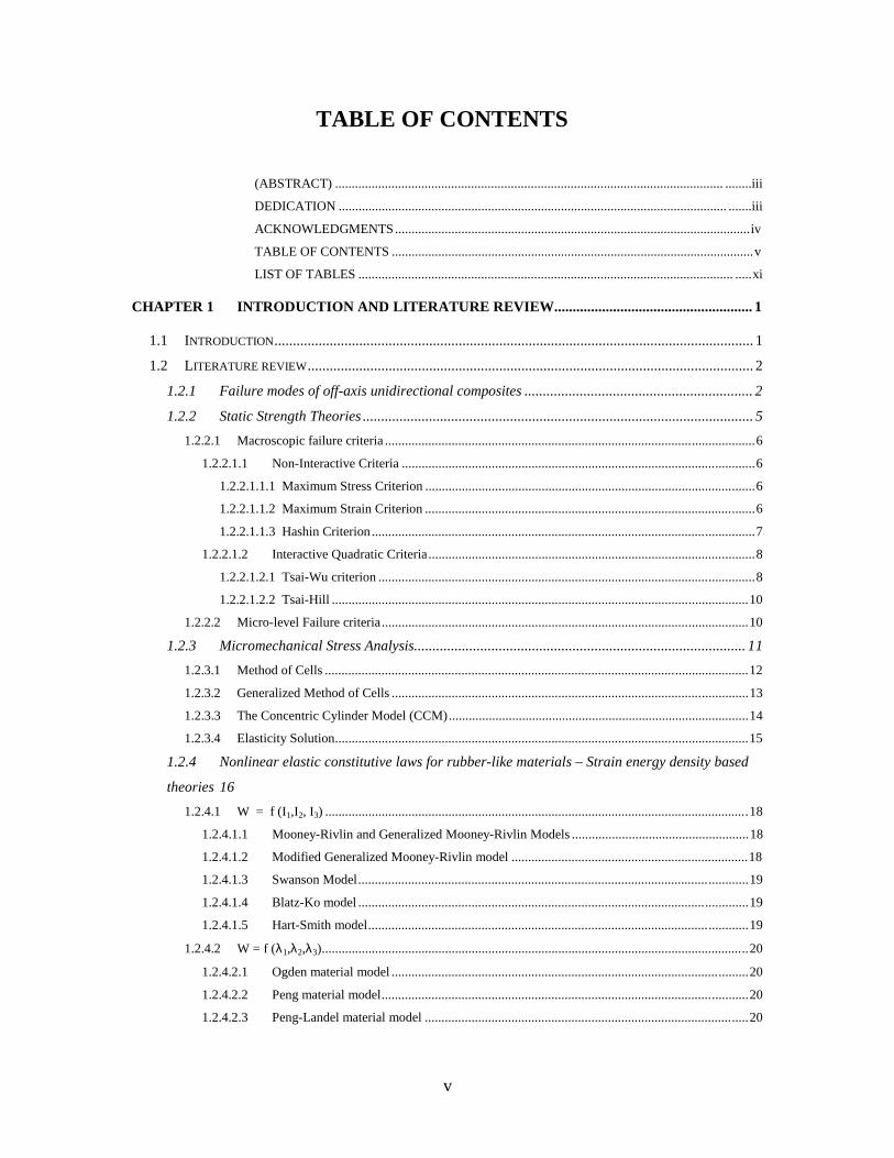
TABLE OF CONTENTS
(ABSTRACT) ..................................................................................................................... ........iii
DEDICATION ..................................................................................................................... .......iii
ACKNOWLEDGMENTS...........................................................................................................iv
TABLE OF CONTENTS .............................................................................................................v
LIST OF TABLES ................................................................................................................. .....xi
CHAPTER 1 INTRODUCTION AND LITERATURE REVIEW...................................................... 1
1.1 INTRODUCTION.................................................................................................................................. 1
1.2 LITERATURE REVIEW......................................................................................................................... 2
1.2.1 Failure modes of off-axis unidirectional composites .............................................................. 2
1.2.2 Static Strength Theories .......................................................................................................... 5
1.2.2.1 Macroscopic failure criteria ...............................................................................................................6
1.2.2.1.1 Non-Interactive Criteria ..........................................................................................................6
1.2.2.1.1.1 Maximum Stress Criterion ...................................................................................................6
1.2.2.1.1.2 Maximum Strain Criterion ...................................................................................................6
1.2.2.1.1.3 Hashin Criterion...................................................................................................................7
1.2.2.1.2 Interactive Quadratic Criteria..................................................................................................8
1.2.2.1.2.1 Tsai-Wu criterion .................................................................................................................8
1.2.2.1.2.2 Tsai-Hill .............................................................................................................................10
1.2.2.2 Micro-level Failure criteria..............................................................................................................10
1.2.3 Micromechanical Stress Analysis.......................................................................................... 11
1.2.3.1 Method of Cells ...............................................................................................................................12
1.2.3.2 Generalized Method of Cells ...........................................................................................................13
1.2.3.3 The Concentric Cylinder Model (CCM)..........................................................................................14
1.2.3.4 Elasticity Solution............................................................................................................................15
1.2.4 Nonlinear elastic constitutive laws for rubber-like materials – Strain energy density based
theories 16
1.2.4.1 W = f (I1,I2, I3) ...............................................................................................................................18
1.2.4.1.1 Mooney-Rivlin and Generalized Mooney-Rivlin Models .....................................................18
1.2.4.1.2 Modified Generalized Mooney-Rivlin model .......................................................................18
1.2.4.1.3 Swanson Model.....................................................................................................................19
1.2.4.1.4 Blatz-Ko model .....................................................................................................................19
1.2.4.1.5 Hart-Smith model..................................................................................................................19
1.2.4.2 W = f (λ1,λ2,λ3)................................................................................................................................20
1.2.4.2.1 Ogden material model ...........................................................................................................20
1.2.4.2.2 Peng material model..............................................................................................................20
1.2.4.2.3 Peng-Landel material model .................................................................................................20
vi
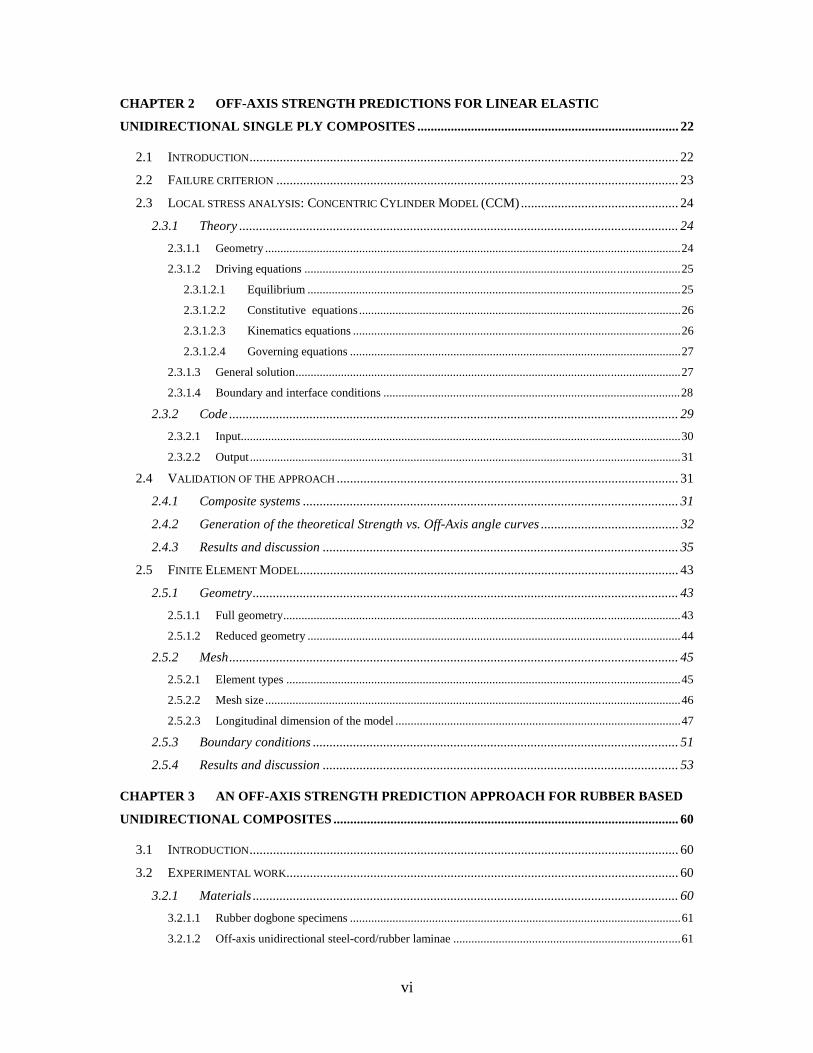
CHAPTER 2 OFF-AXIS STRENGTH PREDICTIONS FOR LINEAR ELASTIC
UNIDIRECTIONAL SINGLE PLY COMPOSITES .............................................................................. 22
2.1 INTRODUCTION................................................................................................................................ 22
2.2 FAILURE CRITERION ........................................................................................................................ 23
2.3 LOCAL STRESS ANALYSIS: CONCENTRIC CYLINDER MODEL (CCM)............................................... 24
2.3.1 Theory ................................................................................................................................... 24
2.3.1.1 Geometry .........................................................................................................................................24
2.3.1.2 Driving equations ............................................................................................................................25
2.3.1.2.1 Equilibrium ...........................................................................................................................25
2.3.1.2.2 Constitutive equations ..........................................................................................................26
2.3.1.2.3 Kinematics equations ............................................................................................................26
2.3.1.2.4 Governing equations .............................................................................................................27
2.3.1.3 General solution...............................................................................................................................27
2.3.1.4 Boundary and interface conditions ..................................................................................................28
2.3.2 Code ...................................................................................................................................... 29
2.3.2.1 Input.................................................................................................................................................30
2.3.2.2 Output ..............................................................................................................................................31
2.4 VALIDATION OF THE APPROACH ...................................................................................................... 31
2.4.1 Composite systems ................................................................................................................ 31
2.4.2 Generation of the theoretical Strength vs. Off-Axis angle curves ......................................... 32
2.4.3 Results and discussion .......................................................................................................... 35
2.5 FINITE ELEMENT MODEL................................................................................................................. 43
2.5.1 Geometry............................................................................................................................... 43
2.5.1.1 Full geometry...................................................................................................................................43
2.5.1.2 Reduced geometry ...........................................................................................................................44
2.5.2 Mesh...................................................................................................................................... 45
2.5.2.1 Element types ..................................................................................................................................45
2.5.2.2 Mesh size .........................................................................................................................................46
2.5.2.3 Longitudinal dimension of the model ..............................................................................................47
2.5.3 Boundary conditions ............................................................................................................. 51
2.5.4 Results and discussion .......................................................................................................... 53
CHAPTER 3 AN OFF-AXIS STRENGTH PREDICTION APPROACH FOR RUBBER BASED
UNIDIRECTIONAL COMPOSITES ....................................................................................................... 60
3.1 INTRODUCTION................................................................................................................................ 60
3.2 EXPERIMENTAL WORK..................................................................................................................... 60
3.2.1 Materials ............................................................................................................................... 60
3.2.1.1 Rubber dogbone specimens .............................................................................................................61
3.2.1.2 Off-axis unidirectional steel-cord/rubber laminae ...........................................................................61

vii
3.2.1.3 +30º/-30º and +18º/-18º steel-cord/rubber laminates .......................................................................62
3.2.2 Description of the experiments.............................................................................................. 62
3.2.3 Experimental results and discussion ..................................................................................... 63
3.2.3.1 Tensile tests on the rubber dogbones ...............................................................................................63
3.2.3.1.1 Engineering stress-strain curve .............................................................................................63
3.2.3.1.2 True stress-strain curve .........................................................................................................65
3.2.3.1.3 Second Piola-Kirchoff stress - Green-Lagrange strain curve ................................................66
3.2.3.2 Tensile tests on the off-axis unidirectional steel-cord/rubber laminae.............................................70
3.2.3.3 Tensile tests on the off-axis unidirectional steel-cord/rubber laminates ..........................................75
3.2.3.4 Strength vs. off-axis angle curve for the laminae and the laminates ................................................77
3.3 THE FINITE ELEMENT MODEL ......................................................................................................... 77
3.3.1 Nonlinear structural analysis in ANSYS - Newton-Raphson procedure ............................... 78
3.3.1.1 Basics...............................................................................................................................................78
3.3.1.2 The Newton-Raphson procedure (from ANSYS Theory Manual)..................................................78
3.3.2 Rubber constitutive relation.................................................................................................. 80
3.3.3 Stress or displacement boundary conditions ?...................................................................... 80
3.3.4 Submodeling.......................................................................................................................... 80
CHAPTER 4 SUMMARY AND CONCLUSIONS............................................................................. 82
4.1 SUMMARY ....................................................................................................................................... 82
4.2 FUTURE WORK................................................................................................................................. 82
4.2.1 Linear analysis...................................................................................................................... 82
4.2.2 Nonlinear analysis ................................................................................................................ 83
REFERENCES...........................................................................................................................84
APPENDIX 1 ….……………………………………………………………………………….89
VITA ……………………………………………………………………………………………93
viii
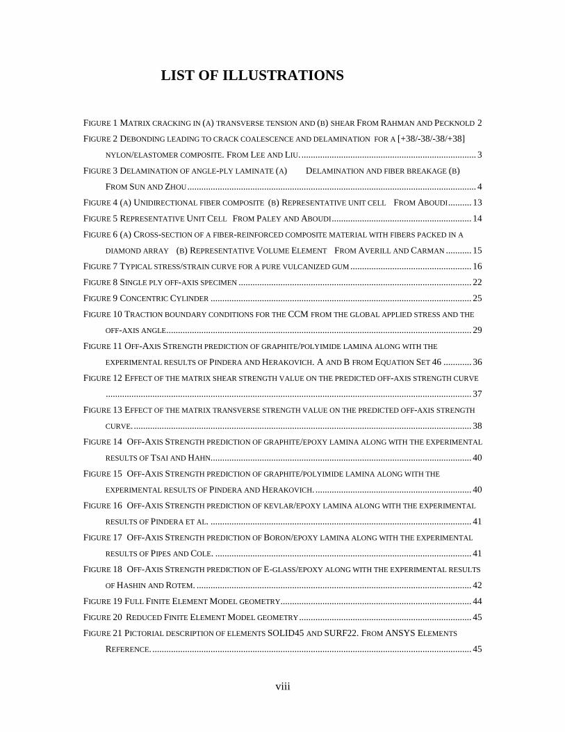
LIST OF ILLUSTRATIONS
FIGURE 1 MATRIX CRACKING IN (A) TRANSVERSE TENSION AND (B) SHEAR FROM RAHMAN AND PECKNOLD 2
FIGURE 2 DEBONDING LEADING TO CRACK COALESCENCE AND DELAMINATION FOR A [+38/-38/-38/+38]
NYLON/ELASTOMER COMPOSITE. FROM LEE AND LIU. ........................................................................... 3
FIGURE 3 DELAMINATION OF ANGLE-PLY LAMINATE (A) DELAMINATION AND FIBER BREAKAGE (B)
FROM SUN AND ZHOU............................................................................................................................ 4
FIGURE 4 (A) UNIDIRECTIONAL FIBER COMPOSITE (B) REPRESENTATIVE UNIT CELL FROM ABOUDI.......... 13
FIGURE 5 REPRESENTATIVE UNIT CELL FROM PALEY AND ABOUDI............................................................ 14
FIGURE 6 (A) CROSS-SECTION OF A FIBER-REINFORCED COMPOSITE MATERIAL WITH FIBERS PACKED IN A
DIAMOND ARRAY (B) REPRESENTATIVE VOLUME ELEMENT FROM AVERILL AND CARMAN ........... 15
FIGURE 7 TYPICAL STRESS/STRAIN CURVE FOR A PURE VULCANIZED GUM .................................................... 16
FIGURE 8 SINGLE PLY OFF-AXIS SPECIMEN .................................................................................................... 22
FIGURE 9 CONCENTRIC CYLINDER ................................................................................................................ 25
FIGURE 10 TRACTION BOUNDARY CONDITIONS FOR THE CCM FROM THE GLOBAL APPLIED STRESS AND THE
OFF-AXIS ANGLE................................................................................................................................... 29
FIGURE 11 OFF-AXIS STRENGTH PREDICTION OF GRAPHITE/POLYIMIDE LAMINA ALONG WITH THE
EXPERIMENTAL RESULTS OF PINDERA AND HERAKOVICH. A AND B FROM EQUATION SET 46 ............ 36
FIGURE 12 EFFECT OF THE MATRIX SHEAR STRENGTH VALUE ON THE PREDICTED OFF-AXIS STRENGTH CURVE
............................................................................................................................................................. 37
FIGURE 13 EFFECT OF THE MATRIX TRANSVERSE STRENGTH VALUE ON THE PREDICTED OFF-AXIS STRENGTH
CURVE.................................................................................................................................................. 38
FIGURE 14 OFF-AXIS STRENGTH PREDICTION OF GRAPHITE/EPOXY LAMINA ALONG WITH THE EXPERIMENTAL
RESULTS OF TSAI AND HAHN................................................................................................................ 40
FIGURE 15 OFF-AXIS STRENGTH PREDICTION OF GRAPHITE/POLYIMIDE LAMINA ALONG WITH THE
EXPERIMENTAL RESULTS OF PINDERA AND HERAKOVICH. ................................................................... 40
FIGURE 16 OFF-AXIS STRENGTH PREDICTION OF KEVLAR/EPOXY LAMINA ALONG WITH THE EXPERIMENTAL
RESULTS OF PINDERA ET AL. ................................................................................................................ 41
FIGURE 17 OFF-AXIS STRENGTH PREDICTION OF BORON/EPOXY LAMINA ALONG WITH THE EXPERIMENTAL
RESULTS OF PIPES AND COLE. .............................................................................................................. 41
FIGURE 18 OFF-AXIS STRENGTH PREDICTION OF E-GLASS/EPOXY ALONG WITH THE EXPERIMENTAL RESULTS
OF HASHIN AND ROTEM. ...................................................................................................................... 42
FIGURE 19 FULL FINITE ELEMENT MODEL GEOMETRY.................................................................................. 44
FIGURE 20 REDUCED FINITE ELEMENT MODEL GEOMETRY.......................................................................... 45
FIGURE 21 PICTORIAL DESCRIPTION OF ELEMENTS SOLID45 AND SURF22. FROM ANSYS ELEMENTS
REFERENCE. ......................................................................................................................................... 45
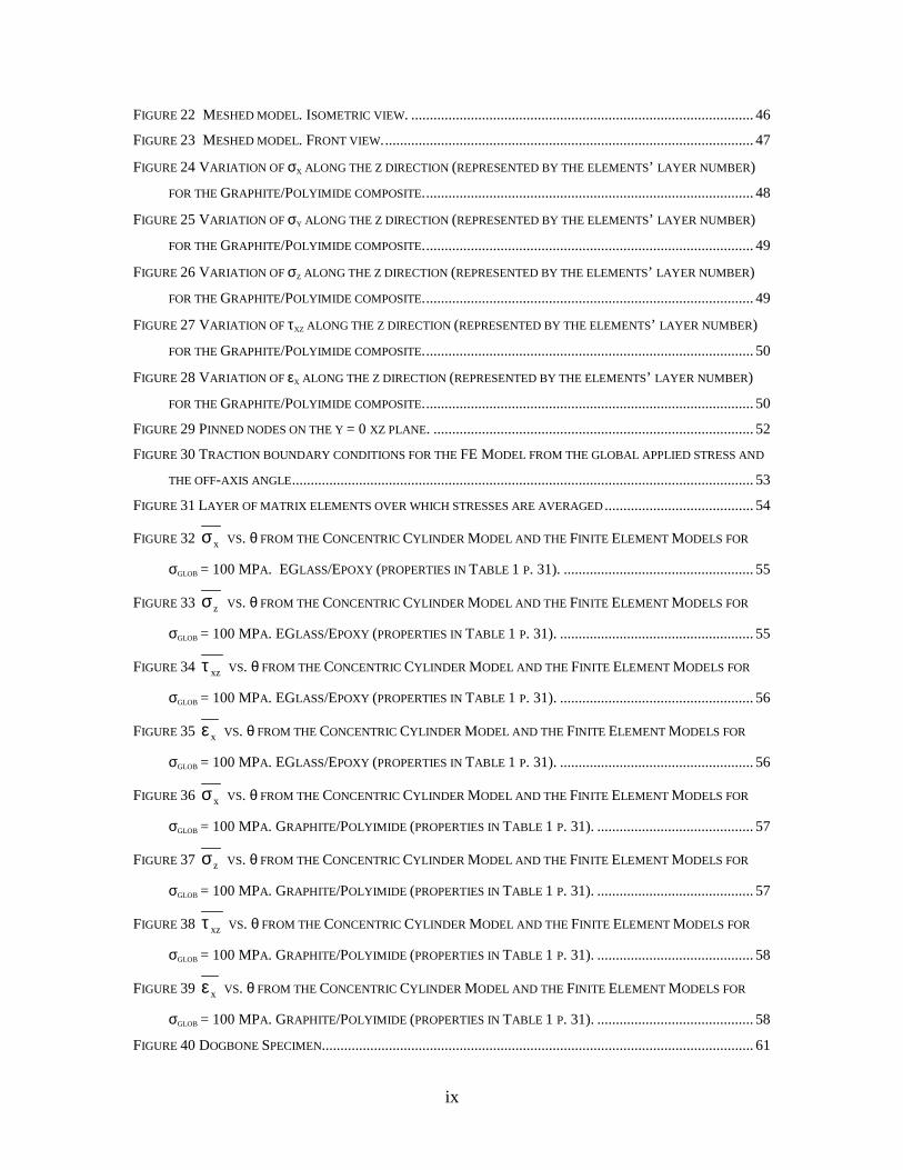
ix
FIGURE 22 MESHED MODEL. ISOMETRIC VIEW. ............................................................................................ 46
FIGURE 23 MESHED MODEL. FRONT VIEW.................................................................................................... 47
FIGURE 24 VARIATION OF σX ALONG THE Z DIRECTION (REPRESENTED BY THE ELEMENTS’ LAYER NUMBER)
FOR THE GRAPHITE/POLYIMIDE COMPOSITE......................................................................................... 48
FIGURE 25 VARIATION OF σY ALONG THE Z DIRECTION (REPRESENTED BY THE ELEMENTS’ LAYER NUMBER)
FOR THE GRAPHITE/POLYIMIDE COMPOSITE......................................................................................... 49
FIGURE 26 VARIATION OF σZ ALONG THE Z DIRECTION (REPRESENTED BY THE ELEMENTS’ LAYER NUMBER)
FOR THE GRAPHITE/POLYIMIDE COMPOSITE......................................................................................... 49
FIGURE 27 VARIATION OF τXZ ALONG THE Z DIRECTION (REPRESENTED BY THE ELEMENTS’ LAYER NUMBER)
FOR THE GRAPHITE/POLYIMIDE COMPOSITE......................................................................................... 50
FIGURE 28 VARIATION OF εX ALONG THE Z DIRECTION (REPRESENTED BY THE ELEMENTS’ LAYER NUMBER)
FOR THE GRAPHITE/POLYIMIDE COMPOSITE......................................................................................... 50
FIGURE 29 PINNED NODES ON THE Y = 0 XZ PLANE. ...................................................................................... 52
FIGURE 30 TRACTION BOUNDARY CONDITIONS FOR THE FE MODEL FROM THE GLOBAL APPLIED STRESS AND
THE OFF-AXIS ANGLE............................................................................................................................ 53
FIGURE 31 LAYER OF MATRIX ELEMENTS OVER WHICH STRESSES ARE AVERAGED ........................................ 54
FIGURE 32 xσ VS. θ FROM THE CONCENTRIC CYLINDER MODEL AND THE FINITE ELEMENT MODELS FOR
σGLOB = 100 MPA. EGLASS/EPOXY (PROPERTIES IN TABLE 1 P. 31). ................................................... 55
FIGURE 33 zσ VS. θ FROM THE CONCENTRIC CYLINDER MODEL AND THE FINITE ELEMENT MODELS FOR
σGLOB = 100 MPA. EGLASS/EPOXY (PROPERTIES IN TABLE 1 P. 31). .................................................... 55
FIGURE 34 xzτ VS. θ FROM THE CONCENTRIC CYLINDER MODEL AND THE FINITE ELEMENT MODELS FOR
σGLOB = 100 MPA. EGLASS/EPOXY (PROPERTIES IN TABLE 1 P. 31). .................................................... 56
FIGURE 35 xε VS. θ FROM THE CONCENTRIC CYLINDER MODEL AND THE FINITE ELEMENT MODELS FOR
σGLOB = 100 MPA. EGLASS/EPOXY (PROPERTIES IN TABLE 1 P. 31). .................................................... 56
FIGURE 36 xσ VS. θ FROM THE CONCENTRIC CYLINDER MODEL AND THE FINITE ELEMENT MODELS FOR
σGLOB = 100 MPA. GRAPHITE/POLYIMIDE (PROPERTIES IN TABLE 1 P. 31). .......................................... 57
FIGURE 37 zσ VS. θ FROM THE CONCENTRIC CYLINDER MODEL AND THE FINITE ELEMENT MODELS FOR
σGLOB = 100 MPA. GRAPHITE/POLYIMIDE (PROPERTIES IN TABLE 1 P. 31). .......................................... 57
FIGURE 38 xzτ VS. θ FROM THE CONCENTRIC CYLINDER MODEL AND THE FINITE ELEMENT MODELS FOR
σGLOB = 100 MPA. GRAPHITE/POLYIMIDE (PROPERTIES IN TABLE 1 P. 31). .......................................... 58
FIGURE 39 xε VS. θ FROM THE CONCENTRIC CYLINDER MODEL AND THE FINITE ELEMENT MODELS FOR
σGLOB = 100 MPA. GRAPHITE/POLYIMIDE (PROPERTIES IN TABLE 1 P. 31). .......................................... 58
FIGURE 40 DOGBONE SPECIMEN.................................................................................................................... 61
x
FIGURE 41 UNIDIRECTIONAL STEEL-CORD/RUBBER LAMINA ......................................................................... 61
FIGURE 42 SIDE VIEW OF +30º/-30º STEEL-CORD/RUBBER SPECIMEN ............................................................ 62
FIGURE 43 INSTRON™ MACHINE ................................................................................................................... 63
FIGURE 44 ENGINEERING STRESS/STRAIN CURVE .......................................................................................... 64
FIGURE 45 MOONEY-RIVLIN BASED PLOT FOR THE RUBBER .......................................................................... 65
FIGURE 46 TRUE STRESS/STRAIN CURVE........................................................................................................ 66
FIGURE 47 DEFORMATION OF THE GAGE PART OF THE RUBBER DOGBONE ..................................................... 67
FIGURE 48 REDUCED GEOMETRY................................................................................................................... 68
FIGURE 49 SECOND PIOLA-KIRCHOFF STRESS VS. GREEN-LAGRANGE STRAIN.............................................. 70
FIGURE 50 BROKEN OFF-AXIS UNIDIRECTIONAL LAMINAE ............................................................................ 71
FIGURE 51 STRESS/STRAIN CURVE FOR THE 15º OFF-AXIS LAMINA................................................................ 72
FIGURE 52 STRESS/STRAIN CURVE FOR THE 18º OFF-AXIS LAMINA................................................................ 72
FIGURE 53 STRESS/STRAIN CURVE FOR THE 30º OFF-AXIS LAMINA................................................................ 73
FIGURE 54 STRESS/STRAIN CURVE FOR THE 45º OFF-AXIS LAMINA................................................................ 73
FIGURE 55 STRESS/STRAIN CURVE FOR THE 60º OFF-AXIS LAMINA................................................................ 74
FIGURE 56 STRESS/STRAIN CURVE FOR THE 90º OFF-AXIS LAMINA................................................................ 74
FIGURE 57 BROKEN +30º/-30º UNIDIRECTIONAL LAMINATE.......................................................................... 75
FIGURE 58 STRESS/STRAIN CURVE FOR THE +18º/-18º OFF-AXIS LAMINATE .................................................. 76
FIGURE 59 STRESS/STRAIN CURVE FOR THE +30/-30º OFF-AXIS LAMINATE ................................................... 76
FIGURE 60 OFF-AXIS STRENGTH FOR THE STEEL-CORD/RUBBER LAMINAE AND LAMINATES.......................... 77
FIGURE 61 NEWTON-RAPHSON METHOD ....................................................................................................... 79
FIGURE 62 SUBMODELING PROCEDURE FOR THE STEEL-CORD/RUBBER LAMINA............................................ 81

xi
LIST OF TABLES
TABLE 1 PROPERTIES OF THE FIVE UNIDIRECTIONAL COMPOSITES USED TO VALIDATE THE ANALYSIS .......... 31
TABLE 2 KIJ CONSTANTS FOR THE FIVE COMPOSITE SYSTEMS ........................................................................ 34
TABLE 3 FINITE ELEMENT MODELS INFORMATION........................................................................................ 51
1
CHAPTER 1 INTRODUCTION AND LITERATURE REVIEW
1.1 Introduction
Because of their high strength-to-weight ratio as well as corrosion and fatigue
resistance, composite materials are a more and more common alternative to traditional
materials such as metals and polymers. They are used in a wide range of applications:
from the automotive and aerospace industry to the sporting goods industry. With this
steady rise in the use of composite materials, failure theories and life prediction tools
have been developed to help the designer and the engineer. Most of these theories are
macromechanical; the composite is modeled as a homogeneous anisotropic material.
They were derived from the ones used for “classical” homogeneous isotropic materials
such as metals. However, to take into account the interaction of the fiber and the matrix
(the fundamental constituents of the composite) and to directly relate the structural
performance to the fundamental make-up of the composite, a micromechanical study is
necessary. The present work focuses on developing a micromechanics-based method to
predict off-axis strength of unidirectional laminae. The understanding of the failure
mechanisms within a lamina is of prime importance since these laminae are building
blocks of the widely used laminated composites. A special local failure function coupled
with a local stress analysis is used for composites with linear elastic constituents. An
approach for off-axis strength prediction of composites with nonlinear matrix is also
discussed.
In the following section, the failure modes of off-axis unidirectional composites are
presented. Static strength failure criteria and existing micromechanical stress analyses are
then briefly reviewed. The last part of the literature review focuses on nonlinear elastic
constitutive laws for rubber.

2
1.2 Literature review
1.2.1 Failure modes of off-axis unidirectional composites
Numerous previous experiments have been performed on off-axis composite
laminae. Aboudi1 worked on an E-Glass/Epoxy lamina under static loading. The same
composite system was used by Hashin and Rotem2 but under cyclic loading. Interestingly
enough, the failure modes observed were similar for both static and oscillatory loadings.
Described in the early work of Rosen and Dow3 and also of Hashin and Rotem2, failure
takes two basic different configurations:
- for small off-axis angles (< θthr), failure occurs due to cumulative fiber failure. An
explanation for this phenomenon is that for small angles, most of the load is carried
by the fibers. As shown by Rosen3, the failure load is then a function of fiber strength
and of matrix and fiber elastic properties. θthr is usually of the order of 1-2 º; the value
of the threshold angle θthr depends on the type of composites tested.
- for larger angles, the failure mode is matrix cracking along the fiber direction. When
the off-axis angle θ increases, matrix shear and transverse stresses increase whereas
fiber stresses decrease. Subramanian4 observed than for an Glass/Epoxy system, when
5º<θ<30º, the matrix failed in shear (Figure 1 (a)) and when θ>30º, normal stresses in
the matrix became dominant and caused final failure (Figure 1 (b)). These
observations are dependent on the nature of the constituents of the composite.
Generally speaking, we can say that rupture is due to combined transverse tensile and
shear stresses.
(a) (b)
Figure 1 Matrix cracking in (a) transverse tension and (b) shear
From Rahman and Pecknold5
3
Hashin and Rotem2 suggest that the fundamental difference between the two
failure modes described (fiber breaking and matrix cracking) makes it reasonable to
assume that the two phenomena are independent of each other.
Several authors6,7,8,9 investigated failure of unidirectional fiber-reinforced laminates
which consist of unidirectional fiber-reinforced laminae stacked together. Ultimate failure
of these laminates usually results from a sequence of events. The first of these events is
the matrix cracking phenomenon at the lamina level discussed before. Huang and Yeoh10
and Lee and Liu11 describe the sequence of events leading to failure as:
- fiber-matrix debonding developing into matrix cracks within a lamina
- coalescence of matrix cracks to form a line crack that turns into an interply crack
- propagation of the interply crack due to interlaminar shear strain, delamination and
final failure
This process is illustrated in Figure 2. It is common to a wide range of composites, from
Graphite/Epoxy to Steel/Rubber. When the fiber/matrix interface is strong, the debonding
phenomenon is skipped and failure occurs within the matrix.
Figure 2 Debonding leading to crack coalescence and delamination
for a [+38/-38/-38/+38] nylon/elastomer composite. From Lee and Liu11.
4
A typical delamination pattern for elastomer based laminates is shown in Figure 3 (a).
(a) (b)
Figure 3 Delamination of angle-ply laminate (a)
Delamination and fiber breakage (b) From Sun and Zhou12
Fiber-matrix debonding, referred to as “socketing”, was first described by Breidenbach
and Lake13,14. Large interlaminar shear strains are developed in angle-ply elastomeric
composites loaded in tension. According to Lee and Liu11, ±19º steel/rubber laminates
exhibit up to 130% interply shear strain when subjected to a global static tensile strain of
10%. For fiber orientations smaller than 30º, angle-ply laminates with non-elastomeric
matrices may exhibit a “mixed” failure mode also called “Partial FB (fiber breakage)” by
Sun and Zhou12. Failure starts as matrix cracking and delamination and then converts to
fiber breakage (Figure 3 (b)). Independence of the two failure mechanisms may not be
assumed for laminates.
The importance of traction free edges has been noted by Lee and Liu11 and Huang
and Yeoh10 for rubber based composites and Sun and Zhou10 for Graphite/Epoxy
systems. Matrix cracking is thought to initiate close to the cord ends because of higher
stress and strain concentrations.
5
1.2.2 Static Strength Theories
Tools to predict failure of laminated composite systems are of prime importance to
the designer or engineer. A constant effort has been made to develop failure criteria
applicable to composite materials. These criteria were, as expected, derived from those
used for “classical” isotropic materials. Special efforts were made to modify the existing
failure functions or to apply them appropriately to take into account the anisotropy in
strength of composites. The failure criterion determines a surface in the stress space
surface called the failure envelope. As for isotropic materials, this envelope defines an
acceptable state of stress for the composite.
In the case of laminates, the global strength of the system will be dependent on the
strength of the individual plies within the laminate. A straightforward and general
procedure for laminate strength analysis exists and is well established. Using Classical
Lamination Theory, stresses in each ply are calculated. The global applied load is
increased till a lamina fails (usually referred to as First Ply Failure: FPF) according to a
predefined criterion. The properties of the failed lamina are then discounted and a new
stress and strain distribution in each lamina is calculated. If we have a stress-controlled
loading condition, the stresses in the undiscounted plies increase to satisfy equilibrium
conditions. The two failure modes normally observed for FPF are delamination and
matrix cracking. The discount operation involves setting the transverse and shear
modulus to a reduced value. When delamination occurs, a single laminate turns into two
or more uncoupled laminates treated in parallel. Other plies may fail at the increased
stress level resulting from FPF. If all of them fail, the laminate is said to have suffered
“gross failure”. If no more laminae fail, the load is increased and the process repeated. As
pointed out by Jones15, “the entire procedure for strength analysis is independent of the
failure criterion, but the results of the procedure, the maximum loads and deformations,
do depend on the specific failure criterion”.
In the next sections, we will survey commonly employed failure criteria. Most of
these criteria are macroscopic, that is, applied at the lamina level. But the use of
microscopic (at the fiber/matrix level) failure criteria, coupled with micromechanics-

6
based analysis is being used increasingly. For an extensive review of existing failure
criteria, the reader is referred to Nahas16.
1.2.2.1 Macroscopic failure criteria
We will use the classification first introduced by Tsai17 who differentiates non-
interactive and interactive criteria. A criterion is said to be interactive when it takes into
account interaction of the different mechanisms and modes of failure.
1.2.2.1.1 Non-Interactive Criteria
1.2.2.1.1.1 Maximum Stress Criterion
Equation Set 1
S S
stresses (-) ecompressivfor Yor stresses )( efor tensil Y
X X
xyxy
cyty
cxtx
<<
>+<
><
where x is the fiber direction, y the transverse direction.
Xt,c = Tensile and Compressive strength in x direction
Yt,c= Tensile and Compressive strength in y direction
S = In-Plane Shear Strength
Failure occurs when one of the inequality is met. To use this criterion, the five previously
defined strengths must be experimentally measured.
1.2.2.1.1.2 Maximum Strain Criterion
This criterion is very similar to maximum stress.
7
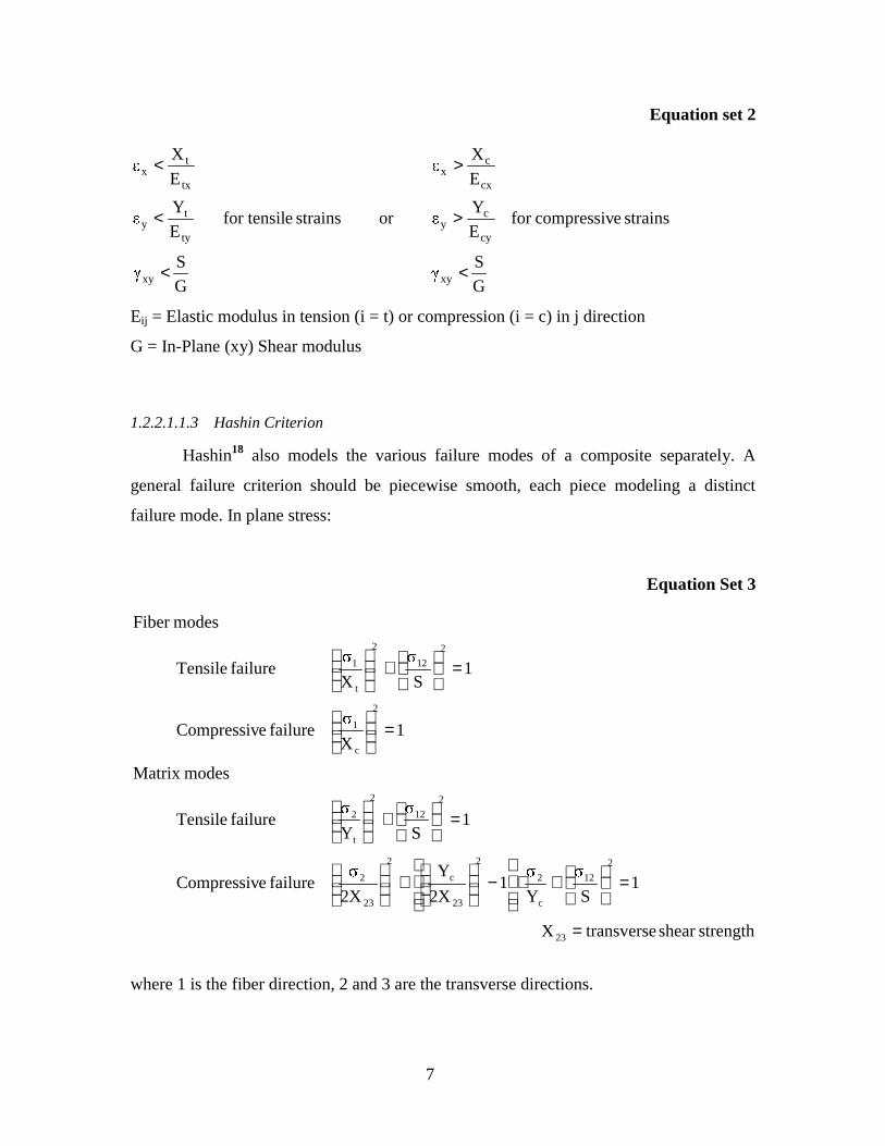
Equation set 2
G
S
G
S
strains ecompressivfor E
Y or strains efor tensil
E
Y
E
X
E
X
xyxy
cy
cy
ty
ty
cx
cx
tx
tx
<<
><
><
Eij = Elastic modulus in tension (i = t) or compression (i = c) in j direction
G = In-Plane (xy) Shear modulus
1.2.2.1.1.3 Hashin Criterion
Hashin18 also models the various failure modes of a composite separately. A
general failure criterion should be piecewise smooth, each piece modeling a distinct
failure mode. In plane stress:
Equation Set 3
strengthshear transverseX
1SY
12X
Y
2X failure eCompressiv
1SY
failure Tensile
modesMatrix
1X
failure eCompressiv
1SX
failure Tensile
modesFiber
23
2
12
c
2
2
23
c
2
23
2
2
12
2
t
2
2
c
1
2
12
2
t
1
=
=
+⋅
−
+
=
+
=
=
+
where 1 is the fiber direction, 2 and 3 are the transverse directions.
8
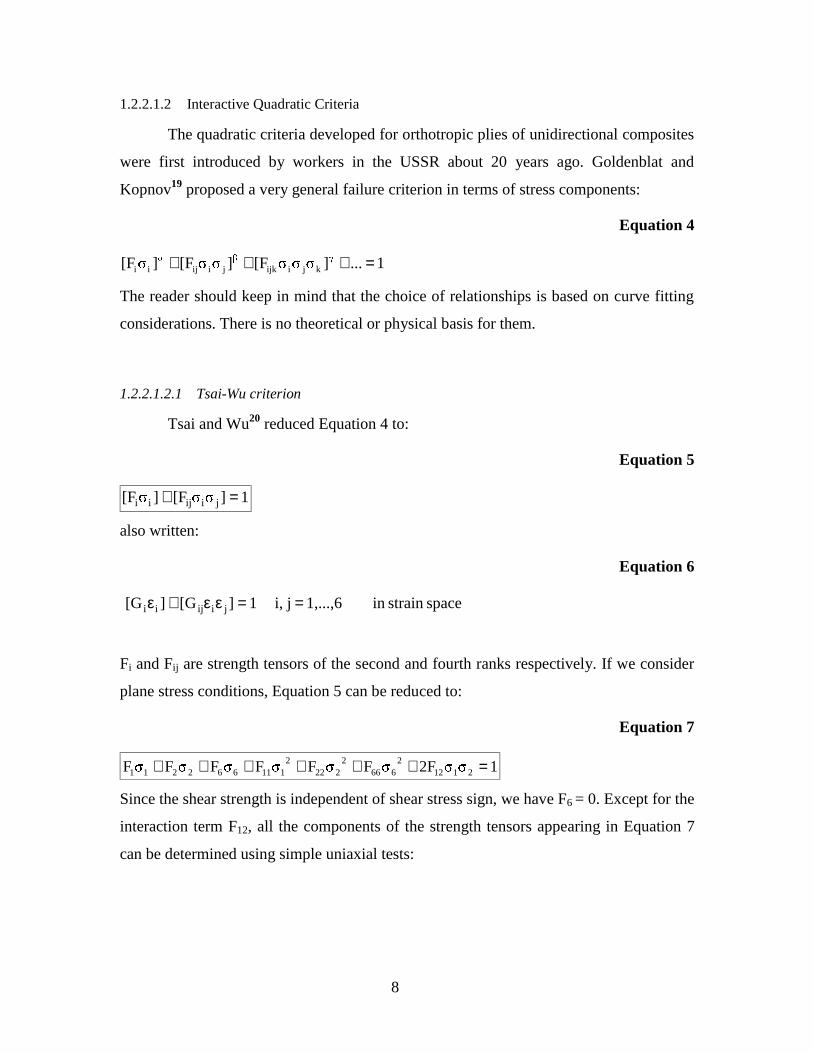
1.2.2.1.2 Interactive Quadratic Criteria
The quadratic criteria developed for orthotropic plies of unidirectional composites
were first introduced by workers in the USSR about 20 years ago. Goldenblat and
Kopnov19 proposed a very general failure criterion in terms of stress components:
Equation 4
1...][F][F][F kjiijkjiijii =+++
The reader should keep in mind that the choice of relationships is based on curve fitting
considerations. There is no theoretical or physical basis for them.
1.2.2.1.2.1 Tsai-Wu criterion
Tsai and Wu20 reduced Equation 4 to:
Equation 5
1][F][F jiijii =+
also written:
Equation 6
space strain in 1,...,6ji, 1][G][G jiijii ==εε+ε
Fi and Fij are strength tensors of the second and fourth ranks respectively. If we consider
plane stress conditions, Equation 5 can be reduced to:
Equation 7
12FFFFFFF 21122
6662
2222
111662211 =++++++
Since the shear strength is independent of shear stress sign, we have F6 = 0. Except for the
interaction term F12, all the components of the strength tensors appearing in Equation 7
can be determined using simple uniaxial tests:
9
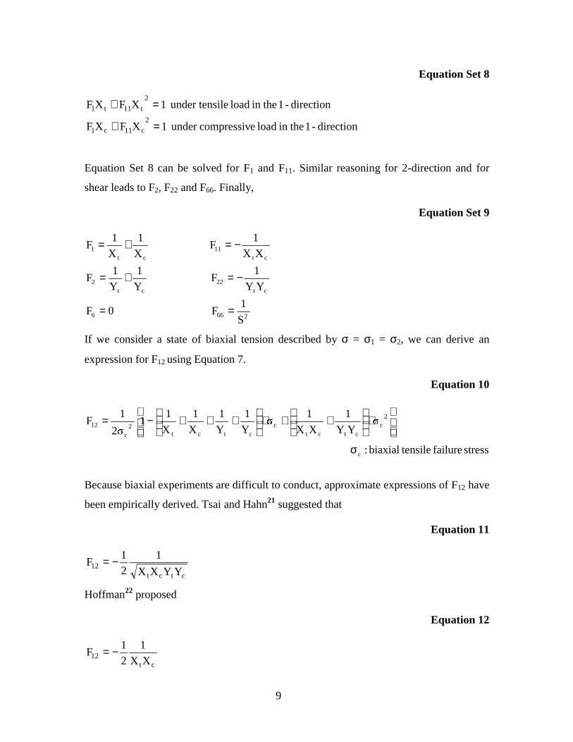
Equation Set 8
direction-1 thein load ecompressivunder 1XFXF
direction-1 thein load ileunder tens 1XFXF2
c11c1
2
t11t1
=+
=+
Equation Set 8 can be solved for F1 and F11. Similar reasoning for 2-direction and for
shear leads to F2, F22 and F66. Finally,
Equation Set 9
2666
ct22
ct2
ct11
ct1
S
1F 0F
YY
1F
Y
1
Y
1F
XX
1F
X
1
X
1F
==
−=+=
−=+=
If we consider a state of biaxial tension described by σ = σ1 = σ2, we can derive an
expression for F12 using Equation 7.
Equation 10
stress failure tensilebiaxial :
YY
1
XX
1
Y
1
Y
1
X
1
X
11
2
1F
c
2c
ctctc
ctct2
c
12
σ
⋅
++⋅
+++−=
Because biaxial experiments are difficult to conduct, approximate expressions of F12 have
been empirically derived. Tsai and Hahn21 suggested that
Equation 11
ctct12
YYXX
1
2
1F −=
Hoffman22 proposed
Equation 12
ct12 XX
1
2
1F −=
10
1.2.2.1.2.2 Tsai-Hill
Tsai23 postulated that the failure criterion of a unidirectional fiber composite has
the same mathematical form as the yield criterion of an orthotropic plastic material. This
yield criterion proposed by Hill24 is based on the Von-Mises criterion for isotropic
materials. The resulting “Tsai-Hill” criterion is:
Equation 13
1F jiij =
It is basically Equation 5 without the linear terms. In plane stress, it is written as:
Equation 14
1SYXX 2
212
2
22
221
2
21 =τ+σ+σσ−σ
1.2.2.2 Micro-level Failure criteria
Most of the failure criteria are phenomenological (macromechanical). There are
very few “local” criteria using mechanistic (micromechanics) analysis. Even though
micromechanics-based analyses have received more and more attention in the recent
years, their main purpose remains as the determination of effective composite properties
from the constituents’ properties. Because interaction of failure mechanisms at the local
(micro) level is thought to be complex to model, local stresses and strains are rarely used
in failure predictions.
However, attempts have been made to use common macroscopic failure theories
at the micro level. Huang25 applied a maximum stress criterion to the constituent
materials of Glass/Epoxy and graphite/Epoxy systems. This criterion was also used by
Rahman and Pecknold5 and by Aboudi1. The results were in good agreement with
experimental data.
Subramanian26 proposed a specific local failure criterion to predict the static
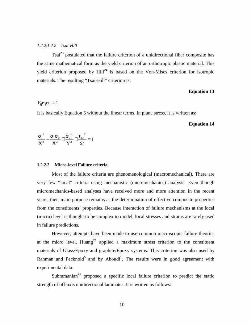
strength of off-axis unidirectional laminates. It is written as follows:
11
failure)(matrix 1SXXX
failure)(fiber X
m
2myz
m
2mzz
m
2myy
m
2mxx
ffzz
=σ
+σ
+σ
+σ
=
where
Xm = In-situ tensile strength of the matrix
Sm = In-situ shear strength of the matrix
Xf = In-situ Tensile Strength of the fiber
stress Averageij =
The stresses were obtained from a Concentric Cylinder Model (See 2.3) and averaged
over the entire volume of the matrix. This approach was extended by Subramanian4 to
predict the fatigue response of unidirectional laminates.
The results and predictions obtained with a failure criterion applied locally are
dependent on the micromechanics model used. This is an important feature of this type of
analysis.
1.2.3 Micromechanical Stress Analysis
Many micromechanics stress analyses based on both analytical and numerical
solutions have been presented in the literature in the past. The Concentric Cylinder Model
is the simplest and the most commonly used. It is a closed-form analysis, but it neglects
the effect of neighboring fibers on the local stress state; therefore, it is expected to work
well for composites with small fiber volume fractions. However, this model was
successfully used to determine effective properties of composites with large volume
fractions. Fiber interactions have been accounted for in models using a regular, periodic
arrangement of the fibers. Common arrangements such as square and hexagonal arrays
were considered. Aboudi1,27 presented theories based on the analysis of a rectilinear
repeating cell representing a unidirectional composite. These theories are referred to as
the Method of Cells and the Generalized Method of Cells.
12
Adams and Doner28 used a finite difference method. Later on, finite element analyses
and boundary element techniques were proposed, respectively, by Adams and Crane29
and by Achenbach and Zu30. The main disadvantages of these numerical solutions are
that they are complex and require large amounts of computing time. To overcome these
problems, analytical solutions have been proposed.
Series-type elasticity solutions are one of the big families of analytical methods. An
extensive review of these elasticity methods is given by Chamis and Sendeckyj31.
Carman and Averill32 developed a refined series-type elasticity solution: it takes into
account all six components of mechanical loading, cylindrical orthotropy of the
constituents and interphase regions. Airy’s stress function approaches were also used,
first by Kobayashi and Ishikawa33,34, and later extended by Naik and Crews35 among
others.
We now present in a more detailed form some of the micromechanical analysis
previously introduced.
1.2.3.1 Method of Cells
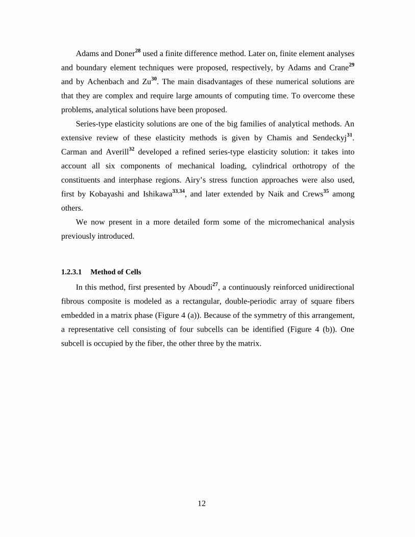
In this method, first presented by Aboudi27, a continuously reinforced unidirectional
fibrous composite is modeled as a rectangular, double-periodic array of square fibers
embedded in a matrix phase (Figure 4 (a)). Because of the symmetry of this arrangement,
a representative cell consisting of four subcells can be identified (Figure 4 (b)). One
subcell is occupied by the fiber, the other three by the matrix.
13
Figure 4 (a) Unidirectional fiber composite (b) Representative unit cell
From Aboudi1
The analysis is performed on the representative cell. The overall behavior of the
composite is determined from the interactions between the subcells. The theory consists
of equilibrium and of continuity of displacements and tractions at the interfaces between
the subcells and between neighboring cells on an average basis. Linear displacement
fields in each subcell are also assumed.
1.2.3.2 Generalized Method of Cells
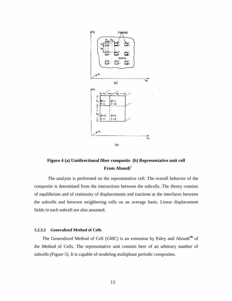
The Generalized Method of Cell (GMC) is an extension by Paley and Aboudi36 of
the Method of Cells. The representative unit consists here of an arbitrary number of
subcells (Figure 5). It is capable of modeling multiphase periodic composites.

14
Figure 5 Representative Unit Cell From Paley and Aboudi36
Compared to the original Method of Cells, the GMC has extended modeling capabilities.
It includes:
- elastic-plastic response of multiphased composites
- modeling of various fiber geometry (both shape and packing arrangements)
- modeling of porosities and damage
- modeling of interfacial regions and inclusions
If accurate, both the Method of Cells and the Generalized Method of Cells require a
considerable amount of calculation. A computer Micromechanics Analysis Code (MAC)
based on the GMC was developed at NASA. It is available at
http://www.lerc.nasa.gov/WWW/LPB/mac/descriptions/index.html.
1.2.3.3 The Concentric Cylinder Model (CCM)
This model was used in the present work. It is discussed in detail in section 2.3
p.24.

15
1.2.3.4 Elasticity Solution
We present here the Averill and Carman32 elasticity solution. They consider a
diamond packed fiber-reinforced composite (Figure 6).
(a)
(b)
Figure 6 (a) Cross-section of a fiber-reinforced composite material with fibers
packed in a diamond array (b) Representative Volume Element
From Averill and Carman32
The fibers have circular cross-section and are of infinite length. Fiber coatings or
interphases may be represented by concentric circular cylinders around the fiber. All
materials are homogeneous and linearly elastic. The matrix is isotropic and the other
phases cylindrically orthotropic.
16
The governing equations of the model are basically the same as those of the
Concentric Cylinder Model (See 2.3 p.24). The solutions of the two models differ
because of the boundary conditions. In the Averill and Carman model, they are:
é No singularity at r = 0.
é Continuity of displacement and normal stress at the fiber matrix interface and
between adjacent cells.
é On the diagonal boundary (See Figure 6 (b)), a collocation technique is applied.
For more details, the reader is referred to the work of Averill and Carman32.
1.2.4 Nonlinear elastic constitutive laws for rubber-like materials – Strain
energy density based theories
Large elastic extensibility or hyperelasticity often characterizes rubber-like
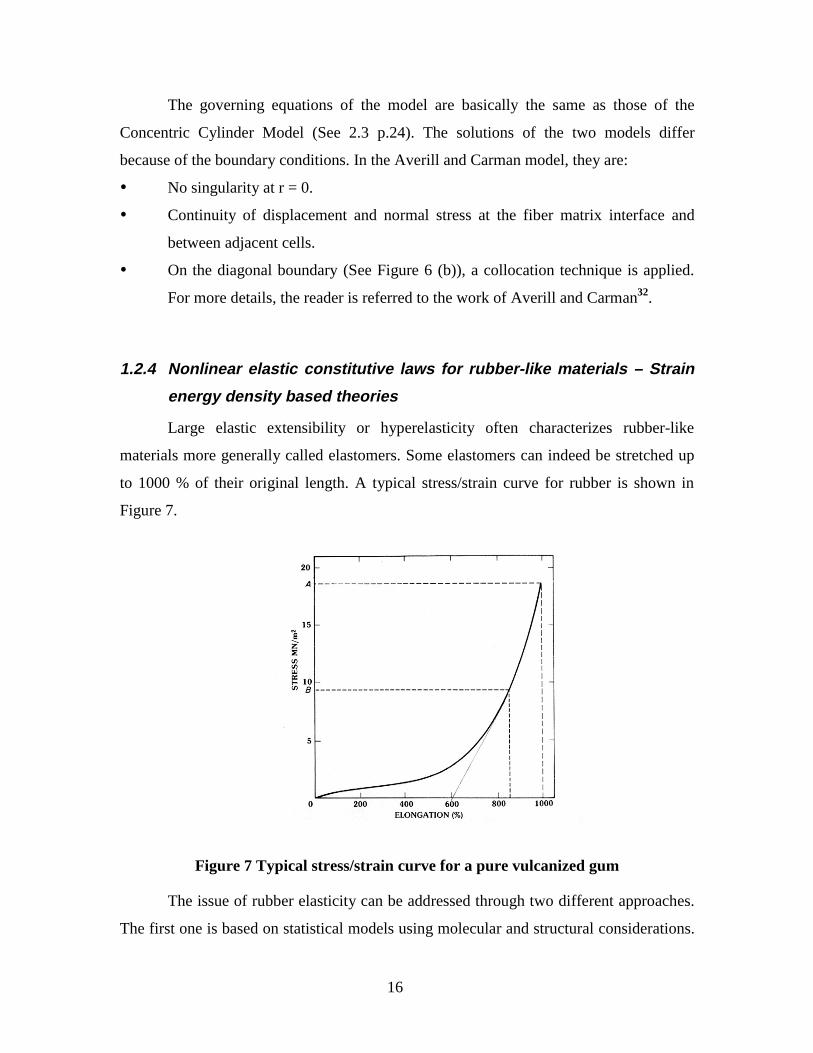
materials more generally called elastomers. Some elastomers can indeed be stretched up
to 1000 % of their original length. A typical stress/strain curve for rubber is shown in
Figure 7.
Figure 7 Typical stress/strain curve for a pure vulcanized gum
The issue of rubber elasticity can be addressed through two different approaches.
The first one is based on statistical models using molecular and structural considerations.
17
Rubber is described as a network of flexible molecular chains that can deform and change
conformation when subjected to a stress. The second approach makes no reference to
molecular structure and assumes that the material is characterized by a purely mechanical
constitutive relation. It is referred to as the continuum theory of rubber elasticity. Because
the present work is mainly mechanics based, this theory is more suitable to our purposes
and will be discussed next.
The continuum theory includes several models; all are based on the strain energy
density function W. Two categories of models can be distinguished. In the first category,
W is written as a polynomial function of the principal strain invariants I1, I2 and I3
defined by:
Equation 15
23
22
213
21
23
23
22
22
212
23
22
211
I
I
I
=
++=
++=
where λ1, λ2 and λ3 are the three principal extension ratios.
In the second category, W is assumed to be a separable function of the extension
ratios λ1, λ2 and λ3. For both categories, the strain tensor is the Lagrangian strain tensor ε
and the stress tensor thermodynamically conjugate to this strain is the second Piola-
Kirchhoff stress tensor σ. It relates to W as follows:
Equation 16
W
∂∂=
The constitutive relation tensor D is written as:
Equation 17
2
2WD
∂∂=
∂∂=
18
1.2.4.1 W = f (I1,I2, I3)
1.2.4.1.1 Mooney-Rivlin and Generalized Mooney-Rivlin Models
For isotropic materials, the strain energy density function is a symmetrical function
of I1, I2 and I3. Rivlin37 showed that all possible forms of W could be represented in terms
of the three invariants. If the material is incompressible, I3 = 1 and W is a function of
only I1 and I2. Oden38 proposed the following form for W:
Equation 18
constants material areC re whe3)(I)3(ICW ijj
2i
0i 0j1ij −−= ∑∑
∞
=
∞
=
The particular form of Equation 18 with only linear terms in I1 and I2 was originally
proposed by Mooney39. It is often called the Mooney-Rivlin equation and written as:
Equation 19
)3I(C)3I(CW 201110 −+−=
Equation 18 is sometimes called the generalized Mooney-Rivlin equation. Equation 18
and Equation 19 are the most widely used constitutive relationship in the stress analysis
of elastomers. The constants appearing in both equations are obtained by curve fitting
experimental data.
1.2.4.1.2 Modified Generalized Mooney-Rivlin model
The modified generalized Mooney-Rivlin model was proposed by Gadala40:
Equation Set 20
1)-2(I-II
1)-(I-II by defined invariants modified are I and I where
3)I()3I(CW
322
31121
j2
i
0i 0j1ij
=
=
−−= ∑∑∞
=
∞
=
19
1.2.4.1.3 Swanson41 Model
Swanson wrote the strain energy density function as:
Equation 21
2
)Ln(IB2Adt
t
g(t)
)b2(1
/3)(I3B
)a2(1
/3)(I3AW 3
1i 1jji
1j
I
0j
b1
2j
1i i
a11i 3
ji
+−+
++
+= ∑ ∑∑ ∫∑
∞
=
∞
=
∞
=
+∞
=
+
where Ai, Bj, ai and bj are material constants and the function g is defined by:
Equation Set 22
∑ ∑ +++−=−=
∞
=
∞
=1i 1jjjir33 )b(1B4)a(1A
3
1
2C where1)C(I)g(I
and χ is the bulk modulus.
1.2.4.1.4 Blatz-Ko42 model
Blatz-Ko proposed:
Equation 23
( )�2-1(
2e a wher)1(I
a
23I
2
1W 2a/
31 =
−+−= −
and µ is a material constant.
1.2.4.1.5 Hart-Smith model43
Hart-Smith used:
Equation 24
⋅+= ∫ −
3
ILnkdIeCW 2
213)(Ik 2
11
where C, k1 and k2 are material constants.

20
The second Piola-Kirchhoff stress tensor σ and he constitutive relation tensor D were
derived by Gadala44 for all the previous models.
1.2.4.2 W = f (λ1,λ2,λ3)
1.2.4.2.1 Ogden material model
Ogden45 expressed the strain energy density function as:
Equation 25
1)(b
cW jb
i
3
1i
m
1j j
j −= ∑∑= =
where cj and bj are materials coefficients and m is fixed by the user to achieve the desired
accuracy.
1.2.4.2.2 Peng46 material model
Peng expressed W as:
Equation 26
)(u)(u)(uW 321 λ+λ+λ=
A detailed expression for u is given by Valanis and Landel47.
1.2.4.2.3 Peng-Landel48 material model
This is the simplest model of hyperelasticity. Only one material constant has to be
specified using experimental data. For incompressible materials, W is expressed as:

21
Equation 27
( ) ( ) ( )∑=
−+−−−=
3
1ii
3i
2iii 4)Ln(
216
1)Ln(
18
1)Ln(
6
1)Ln(1cW
where c is the initial tensile modulus.
Methods of developing the materials constants in the previous models from experimental
data are demonstrated by Finney and Kumar49.
22
CHAPTER 2 OFF-AXIS STRENGTH PREDICTIONS FOR
LINEAR ELASTIC UNIDIRECTIONAL SINGLE PLY
COMPOSITES
2.1 Introduction
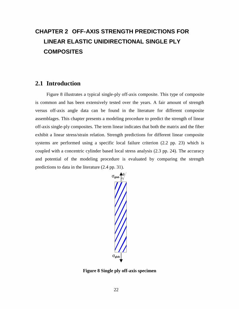
Figure 8 illustrates a typical single-ply off-axis composite. This type of composite
is common and has been extensively tested over the years. A fair amount of strength
versus off-axis angle data can be found in the literature for different composite
assemblages. This chapter presents a modeling procedure to predict the strength of linear
off-axis single-ply composites. The term linear indicates that both the matrix and the fiber
exhibit a linear stress/strain relation. Strength predictions for different linear composite
systems are performed using a specific local failure criterion (2.2 pp. 23) which is
coupled with a concentric cylinder based local stress analysis (2.3 pp. 24). The accuracy
and potential of the modeling procedure is evaluated by comparing the strength
predictions to data in the literature (2.4 pp. 31).
θσglob
σglob
Figure 8 Single ply off-axis specimen
23
A model developed with a commercial finite element code (ANSYS) is also presented in
this chapter (2.5 pp. 43). The results from the Concentric Cylinder Model based code
were verified using the code NDSANDS written by Pagano. The CCM solution was used
to check the finite elements results. The objective was to obtain a Finite Element Model
(FEM) leading to stresses and strains comparable to the ones obtained with CCM (at least
in an average sense). The resulting FEM was then used as a core to develop a nonlinear
model (CHAPTER 3). This nonlinear version is later adopted in the strength prediction
procedure of nonlinear single-ply composites. Indeed, for nonlinear materials, the
Concentric Cylinder Model is not valid anymore and finite element methods are
commonly employed in the absence of any analytical models.
2.2 Failure criterion
The type of composite considered and more importantly the failure mode(s)
encountered serve as guidelines to choose an adequate failure criterion. In off-axis
composites, for angles greater than the threshold angle θthr under which fiber failure takes
place, failure is defined by matrix failure due to combined transverse and shear stresses
(See 1.2.1 pp. 2). Based on our experimental observations and results presented in the
literature (1.2.1 pp. 2), a few assumptions were made. First we will assume that interfaces
between the fibers and the matrix are strong. In this case, failure occurs due to cracking in
the matrix close to the interface (the exact location is not known) along a plane parallel to
the fiber direction. Since the largest matrix stresses and strains occur at the interface and
since failure is not interfacial, we can assume that failure is not controlled by point stress
and/or strain values. As a result, we will employ a local failure criterion using matrix-
averaged values of stresses and strains as opposed to point values. To keep the criterion
as simple as possible, we only use contributions in shear and transverse directions in
the plane of the lamina since cracking results from combined stresses in these two
directions. We will also assume that the life of the composite is controlled by the
initiation of the matrix cracks. In other words, the failure strength corresponds to the
initiation stress; propagation of the cracks is assumed to be quasi-immediate. The
proposed failure criterion is then a crack initiation criterion.
24
One of the objectives of this work was to construct a criterion that would work for
both linear and nonlinear materials. Energy-based failure functions are known to be more
effective for nonlinear materials. Inspired by a paper by Plumtree50, the idea was to
multiply the stress terms by the corresponding strain value to obtain energy terms.
To get a value for the failure criterion between 0 and 1, both the transverse and shear
terms have to be normalized. The proposed failure criterion has the form of a reduced
and normalized strain energy density function:
Equation 28
BAFa xzxzxxxx ⋅+⋅=
where bars indicate matrix-averaged quantities, z is the fiber direction, x is the transverse
direction and A and B are the normalizing constants.
Since stresses and strains in Equation 28 are local, A and B are the products of in-
situ strength and in-situ strain-to-failure of the matrix in the direction of interest. The
method used to obtain A and B is discussed in 2.4.3 p. 35.
2.3 Local stress analysis: Concentric Cylinder Model (CCM)
Several papers address the problem of computation of local stresses in
unidirectional continuous fiber composites subjected to thermo-mechanical loadings and
prediction of its effective stiffness. Several of these papers use models where the
composite constituents are represented by cylinders. The papers by Pagano51,52 present
the advantage of giving a clear and general formulation of a Concentric Cylinder based
model. This formulation will be used in the present work in a simplified version.
2.3.1 Theory
2.3.1.1 Geometry
A continuous fiber reinforced composite is modeled by a representative volume
element composed of two concentric cylinder elements in which the inner cylinder is the
25
fiber and the outer ring is the matrix (Figure 9). The ratio of the two radii is calculated
form the fiber volume fraction. The fiber-to-fiber interaction is neglected in the
Concentric Cylinder Model.
matrix theof radius outerr
fiber theof radiusr where
r
rfraction volumefiber
volumeTotal
fiber of Volume
m
f
2
m
f
==
==
FiberMatrix
x
y
z
r
α
S2
S1
S1
Figure 9 Concentric Cylinder
2.3.1.2 Driving equations
Both the fiber and the matrix are assumed to be linear elastic and homogeneous.
The fiber is assumed to be perfectly bonded to the matrix. The constituent materials have
transversely isotropic properties.
2.3.1.2.1 Equilibrium
The equilibrium equations in cylindrical coordinate system are:
26
Equation set 29
0r
1
r
1
0r
2
r
1
0)(r
1
r
1
rzz,rz,r
r,,r
r,rr,r
=⋅+⋅+
=⋅+⋅+
=−⋅+⋅+
αα
ααααα
ααα
Stresses are only functions of r and α and differentiation is indicated by a comma.
2.3.1.2.2 Constitutive equations
For each constituent material:
Equation set 30
rz55rz
z55z
r44r
22r23z12z
23r22z12r
12r12z11z
C
C
C
CCC
CCC
CCC
⋅=⋅=⋅=
⋅+⋅+⋅=⋅+⋅+⋅=⋅+⋅+⋅=
αα
αα
α
α
α
where Cmn (m, n = 1 , 2 , … , 6) are the elastic stiffness constants of the individual
material.
For transversely isotropic material, 2
CCC 2322
44
−=
2.3.1.2.3 Kinematics equations
27
Equation set 31
rz,zr,rzr,
z,z,z,rr,r
r,r,rzz,z
uu ur
1u
r
1
uur
1 u
ur
1uu
r
1 u
+=⋅+⋅=
+⋅==
⋅−+⋅==
ααα
ααα
αααα
2.3.1.2.4 Governing equations
Substituting Equation set 30 and Equation set 31 into Equation set 29, we obtain
the governing field equation in terms of displacements (ur, uα, uz):
Equation set 32
0)ur
1u
r
1uu
r
1u
r
1u(C
0uC
ur
1)CC(u
r
1)CC(u
r
1C)u
r
1u
r
1u(C
0uC
ur
1)CC(u
r
1)CC(u
r
1C)u
r
1u
r
1u(C
,z2r,zrr,zz,z,rrz,r55
z,z12
,r24422r,r4423,2222r,rr,44
rz,z12
,24422r,4423,r244r2r,rrr,r22
=+++++⋅
=+
⋅++⋅++⋅+−+⋅
=+
⋅+−⋅++⋅+−+⋅
αααα
α
αααααααα
αααααα
2.3.1.3 General solution
The general solution of Equation set 32 is a series solution. A solution containing
the terms necessary to satisfy the class of boundary conditions that are imposed (See
2.3.1.4) is as follows:
28
Equation Set 33
)r(Wzcosz)r(Wsinz)r(W
cos(r)Wsin(r)W(r)W2cos(r)W2sin(r)W)z,,r(u
)r(Vzcosz)r(Vsinz)r(Vcosz)r(Vsinz)r(V
cos(r)Vsin(r)V(r)V2cos(r)V2sin(r)V)z,,r(u
insz)r(Ucosz)r(Uinsz)r(Ucosz)r(U
sin(r)Ucos(r)U(r)Usin2(r)Ucos2(r)U)z,,r(u
1076
(k)5
(k)4
(k)3
(k)2
(k)1
(k)
102
92
876
(k)5
(k)4
(k)3
(k)2
(k)1
(k)
29
2876
(k)5
(k)4
(k)3
(k)2
(k)1
(k)r
⋅+α⋅⋅+α⋅⋅+α⋅+α⋅++α⋅+α⋅=θ
⋅+α⋅⋅+α⋅⋅+α⋅⋅+α⋅⋅
+α⋅+α⋅++α⋅+α⋅=θ
α⋅⋅+α⋅⋅+α⋅⋅+α⋅⋅
+α⋅+α⋅++α⋅+α⋅=θ
θ
θ
where U1(k)(r), U2
(k)(r), … W10(k)(r) are defined in Appendix 1. Using Equation set 30 and
Equation set 31, the stress field is then expressed as:
Equation Set 34
α⋅+α⋅++α⋅+α⋅=
α⋅+α⋅++α⋅+α⋅=
α⋅+α⋅++α⋅+α⋅=
α⋅+α⋅++α⋅+α⋅=
α⋅+α⋅++α⋅+α⋅=
α⋅+α⋅++α⋅+α⋅=
α
α
α
cos(r)sin(r)(r)cos2(r)sin2(r)
sin(r)cos(r)(r)sin2(r)cos2(r)
cos(r)sin(r)(r)cos2(r)sin2(r)
sin(r)cos(r)(r)sin2(r)cos2(r)
sin(r)cos(r)(r)sin2(r)cos2(r)
sin(r)cos(r)(r)sin2(r)cos2(r)
(k)5
(k)4
(k)3
(k)2
(k)1
(k)rz
(k)5
(k)4
(k)3
(k)2
(k)1
(k)z
(k)5
(k)4
(k)3
(k)2
(k)1
(k)r
(k)5
(k)4
(k)3
(k)2
(k)1
(k)
(k)5
(k)4
(k)3
(k)2
(k)1
(k)r
(k)5
(k)4
(k)3
(k)2
(k)1
(k)z
where k = 1, 2 (fiber, matrix) and α1(k)(r), …, δ5
(k)(r) are defined in Appendix 1.
2.3.1.4 Boundary and interface conditions
To solve for the constants A1(k), …, Y3
(k) used to define α1(k)(r), …, δ5
(k)(r) (See
Appendix 1), we have to prescribe interface and boundary conditions. Two types of
boundary conditions can be prescribed on the outer surfaces of our model: displacement
based51 or traction based52 boundary conditions. We chose to apply traction based
conditions to be consistent with the Finite Element model. The surface tractions
employed in the FE model were also derived from the global applied stress and the off-
axis angle.
Finally, the conditions to prescribe are:
(i) Continuity of displacements and stresses across the fiber/matrix interface
29
(ii) Non-singular displacements and stresses at the origin
(iii) Elimination of rigid body motion
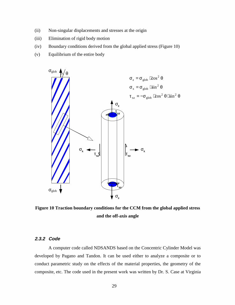
(iv) Boundary conditions derived from the global applied stress (Figure 10)
(v) Equilibrium of the entire body
σglob
σx
σz
σz
σxτxz
τxz
τxz
τxz
θ
σglob
θ⋅θ⋅σ−=τ
θ⋅σ=σ
θ⋅σ=σ
22globxz
2globx
2globz
sincos
sin
cos
Figure 10 Traction boundary conditions for the CCM from the global applied stress
and the off-axis angle
2.3.2 Code
A computer code called NDSANDS based on the Concentric Cylinder Model was
developed by Pagano and Tandon. It can be used either to analyze a composite or to
conduct parametric study on the effects of the material properties, the geometry of the
composite, etc. The code used in the present work was written by Dr. S. Case at Virginia

30
Tech based on the papers by Pagano. This program was modified to calculate the average
stress in the matrix in the x, y and z directions:
Equation 35
dV ),r(V
1
v
ijij ∫∫∫ ασ⋅=σ
where V is the volume of the matrix
σij(r,α) are stresses in the (x,y,z) coordinate system transformed from
Equation Set 34
σij are not z dependent and the cylinders have two axes of symmetry. Equation 35 can
then be reduced to:
Equation 36
∫ ∫=
=
π=α
=α
α⋅⋅⋅ασ⋅=σm
f
rr
rr
2
0
ijij ddrr),r(A
1
2.3.2.1 Input
The code is written in FORTRAN and uses two input files:
· “Prop” is a database of properties of fiber and matrix materials. This file can be
modified by the user and new materials can be added. The properties to be entered are the
elastic constants (longitudinal and transverse Young’s modulus, Poisson’s ratios and
shear modulus), the coefficients of thermal expansion and the coefficients of moisture
absorption.
· “Composit” is a database of composite systems. For each of these systems, the fiber
and matrix materials have to be chosen from the “Prop” database.
The composite to be analyzed, the temperature, the moisture and the applied stresses or
strains are entered interactively when the executable file is run.
31
2.3.2.2 Output
The calculated volume averaged stresses and strains in the matrix are given in an
interactive window.
2.4 Validation of the approach
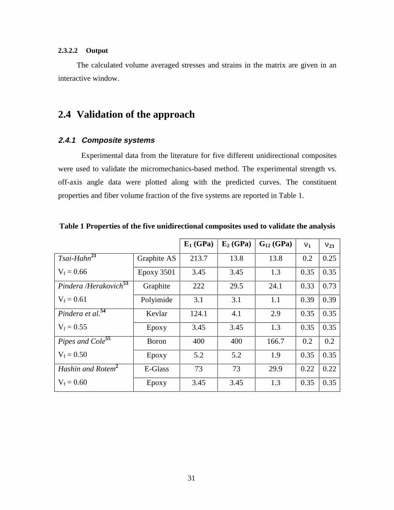
2.4.1 Composite systems
Experimental data from the literature for five different unidirectional composites
were used to validate the micromechanics-based method. The experimental strength vs.
off-axis angle data were plotted along with the predicted curves. The constituent
properties and fiber volume fraction of the five systems are reported in Table 1.
Table 1 Properties of the five unidirectional composites used to validate the analysis
E1 (GPa) E2 (GPa) G12 (GPa) ν1 ν23
Graphite AS 213.7 13.8 13.8 0.2 0.25Tsai-Hahn21
Vf = 0.66 Epoxy 3501 3.45 3.45 1.3 0.35 0.35
Graphite 222 29.5 24.1 0.33 0.73Pindera /Herakovich53
Vf = 0.61 Polyimide 3.1 3.1 1.1 0.39 0.39
Kevlar 124.1 4.1 2.9 0.35 0.35Pindera et al.54
Vf = 0.55 Epoxy 3.45 3.45 1.3 0.35 0.35
Boron 400 400 166.7 0.2 0.2Pipes and Cole55
Vf = 0.50 Epoxy 5.2 5.2 1.9 0.35 0.35
E-Glass 73 73 29.9 0.22 0.22Hashin and Rotem2
Vf = 0.60 Epoxy 3.45 3.45 1.3 0.35 0.35
32
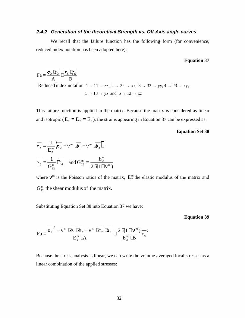
2.4.2 Generation of the theoretical Strength vs. Off-Axis angle curves
We recall that the failure function has the following form (for convenience,
reduced index notation has been adopted here):
Equation 37
xz126 and yz135
,xy234 ,yy333 xx,222 ,zz111 :notationindex Reduced
BA
Fa 6622
→→→→
→→→→→→→→
⋅+⋅=
This failure function is applied in the matrix. Because the matrix is considered as linear
and isotropic ( 321 EEE == ), the strains appearing in Equation 37 can be expressed as:
Equation Set 38
( )
)(12
EG and
G
1
E
1
m
m2m
126m12
6
3m
1m
2m2
2
ν+⋅=⋅=
⋅ν−⋅ν−=
where νm is the Poisson ratios of the matrix, m2E the elastic modulus of the matrix and
matrix. theof modulusshear theG m12
Substituting Equation Set 38 into Equation 37 we have:
Equation 39
2
6m2
m
m2
32m
21m2
2
BE
)(12
AEFa
⋅ν+⋅+
⋅⋅⋅ν−⋅⋅ν−
=
Because the stress analysis is linear, we can write the volume averaged local stresses as a
linear combination of the applied stresses:
33
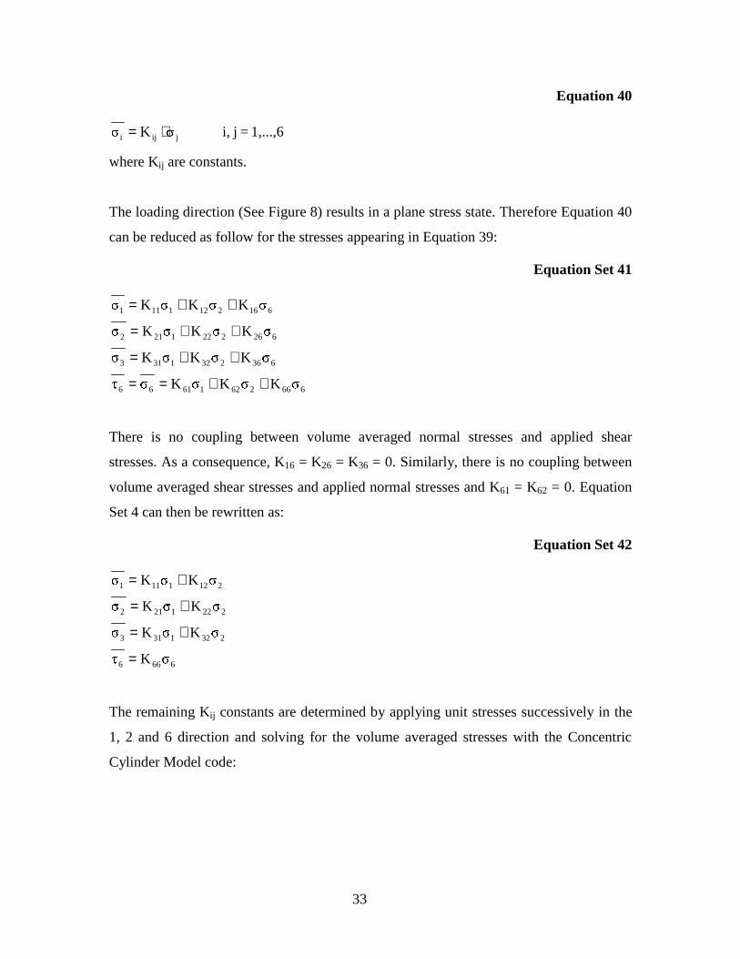
Equation 40
1,...,6=ji, K jiji ⋅=
where Kij are constants.
The loading direction (See Figure 8) results in a plane stress state. Therefore Equation 40
can be reduced as follow for the stresses appearing in Equation 39:
Equation Set 41
66626216166
6362321313
6262221212
6162121111
KKK
KKK
KKK
KKK
++==
++=
++=
++=
There is no coupling between volume averaged normal stresses and applied shear
stresses. As a consequence, K16 = K26 = K36 = 0. Similarly, there is no coupling between
volume averaged shear stresses and applied normal stresses and K61 = K62 = 0. Equation
Set 4 can then be rewritten as:
Equation Set 42
6666
2321313
2221212
2121111
K
KK
KK
KK
=
+=
+=
+=
The remaining Kij constants are determined by applying unit stresses successively in the
1, 2 and 6 direction and solving for the volume averaged stresses with the Concentric
Cylinder Model code:
34
Equation Set 43
666
216
323
222
121
612
313
212
111
621
K=
0 1, 3
K=
K=
K=
0 1, 2
K=
K=
K=
0 1, 1
⇒
===
⇒
===
⇒
===
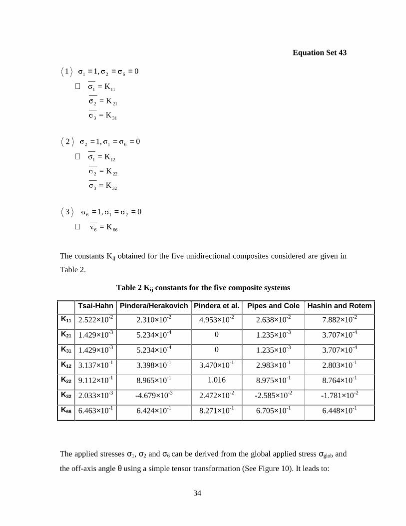
The constants Kij obtained for the five unidirectional composites considered are given in
Table 2.
Table 2 Kij constants for the five composite systems
Tsai-Hahn Pindera/Herakovich Pindera et al. Pipes and Cole Hashin and Rotem
K11 2.522×10⁻² 2.310×10⁻² 4.953×10⁻² 2.638×10⁻² 7.882×10⁻²
K21 1.429×10⁻³ 5.234×10⁻⁴ 0 1.235×10⁻³ 3.707×10⁻⁴
K31 1.429×10⁻³ 5.234×10⁻⁴ 0 1.235×10⁻³ 3.707×10⁻⁴
K12 3.137×10⁻¹ 3.398×10⁻¹ 3.470×10⁻¹ 2.983×10⁻¹ 2.803×10⁻¹
K22 9.112×10⁻¹ 8.965×10⁻¹ 1.016 8.975×10⁻¹ 8.764×10⁻¹
K32 2.033×10⁻³ -4.679×10⁻³ 2.472×10⁻² -2.585×10⁻² -1.781×10⁻²
K66 6.463×10⁻¹ 6.424×10⁻¹ 8.271×10⁻¹ 6.705×10⁻¹ 6.448×10⁻¹
The applied stresses σ1, σ2 and σ6 can be derived from the global applied stress σglob and
the off-axis angle θ using a simple tensor transformation (See Figure 10). It leads to:
35
Equation Set 44
)sin()cos(
)(sin
)(cos
glob6
2glob2
2glob1
θθ⋅σ−=τ
θ⋅σ=σ
θ⋅σ=σ
Substituting Equation Set 42 then Equation Set 44 into Equation 39, we obtain:
Equation 45
( )( ) ( )( ) ( )
θ+θ⋅θ+θ⋅ν−
θ+θ⋅θ+θ⋅ν−
θ+θ
⋅σ=
)(sinK)(cosK)(sinK)(cosK
)(sinK)(cosK)(sinK)(cosK
)(sinK)(cosK
AE
1Fa
222
221
232
231
m
222
221
212
211
m
2222
221
m2
2
glob
θθ⋅
⋅ν+⋅+ )(sin)(cosKBE
)1(2 222
66m2
m
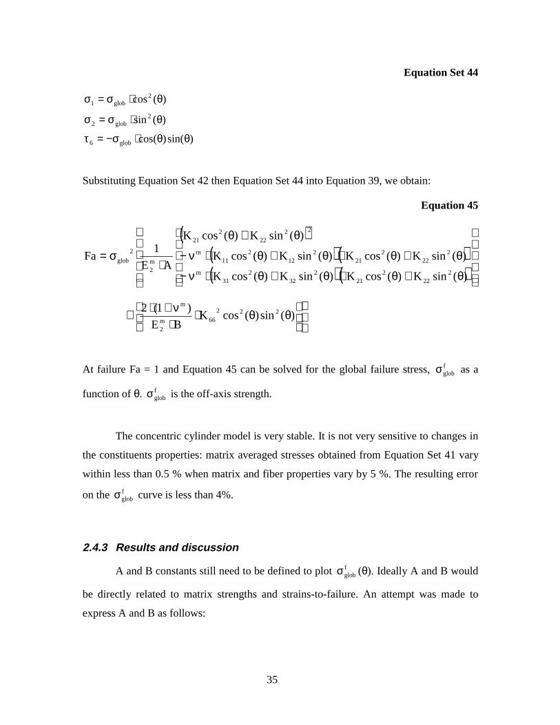
At failure Fa = 1 and Equation 45 can be solved for the global failure stress, σglobf as a
function of θ. σglobf is the off-axis strength.
The concentric cylinder model is very stable. It is not very sensitive to changes in
the constituents properties: matrix averaged stresses obtained from Equation Set 41 vary
within less than 0.5 % when matrix and fiber properties vary by 5 %. The resulting error
on the σglobf curve is less than 4%.
2.4.3 Results and discussion
A and B constants still need to be defined to plot σglobf (θ). Ideally A and B would
be directly related to matrix strengths and strains-to-failure. An attempt was made to
express A and B as follows:
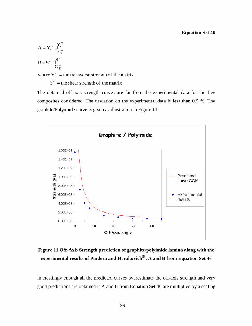
36
Equation Set 46
matrix theof strengthshear the S
matrix theof strength e transversthe Ywhere
G
SSB
E
YYA
m
mt
m12
mm
m2
mtm
t
=
=
⋅=
⋅=
The obtained off-axis strength curves are far from the experimental data for the five
composites considered. The deviation on the experimental data is less than 0.5 %. The
graphite/Polyimide curve is given as illustration in Figure 11.
*UDSKLWH���3RO\LPLGH
0.00E+00
2.00E+08
4.00E+08
6.00E+08
8.00E+08
1.00E+09
1.20E+09
1.40E+09
1.60E+09
0 20 40 60 80
Off-Axis angle
Str
eng
th (
Pa) Predicted
curve CCM
Experimentalresults
Figure 11 Off-Axis Strength prediction of graphite/polyimide lamina along with the
experimental results of Pindera and Herakovich53. A and B from Equation Set 46
Interestingly enough all the predicted curves overestimate the off-axis strength and very
good predictions are obtained if A and B from Equation Set 46 are multiplied by a scaling
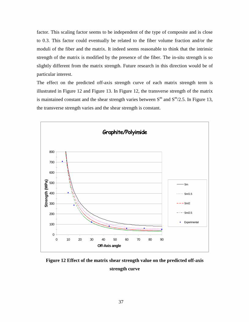
37
factor. This scaling factor seems to be independent of the type of composite and is close
to 0.3. This factor could eventually be related to the fiber volume fraction and/or the
moduli of the fiber and the matrix. It indeed seems reasonable to think that the intrinsic
strength of the matrix is modified by the presence of the fiber. The in-situ strength is so
slightly different from the matrix strength. Future research in this direction would be of
particular interest.
The effect on the predicted off-axis strength curve of each matrix strength term is
illustrated in Figure 12 and Figure 13. In Figure 12, the transverse strength of the matrix
is maintained constant and the shear strength varies between Sm and Sm/2.5. In Figure 13,
the transverse strength varies and the shear strength is constant.
*UDSKLWH�3RO\LPLGH
0
100
200
300
400
500
600
700
800
0 10 20 30 40 50 60 70 80 90
Off-Axis angle
Str
eng
th (
MP
a)
Sm
Sm/1.5
Sm/2
Sm/2.5
Experimental
Figure 12 Effect of the matrix shear strength value on the predicted off-axis
strength curve
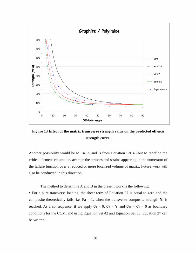
38
*UDSKLWH���3RO\LPLGH�
0
100
200
300
400
500
600
700
800
0 10 20 30 40 50 60 70 80 90
Off-Axis angle
Str
eng
th (
MP
a)
Ytm
Ytm/1.5
Ytm/2
Ytm/2.5
Experimental
Figure 13 Effect of the matrix transverse strength value on the predicted off-axis
strength curve.
Another possibility would be to use A and B from Equation Set 46 but to redefine the
critical element volume i.e. average the stresses and strains appearing in the numerator of
the failure function over a reduced or more localized volume of matrix. Future work will
also be conducted in this direction.
The method to determine A and B in the present work is the following:
é For a pure transverse loading, the shear term of Equation 37 is equal to zero and the
composite theoretically fails, i.e. Fa = 1, when the transverse composite strength Yt is
reached. As a consequence, if we apply σ1 = 0, σ2 = Yt and σ12 = σ6 = 0 as boundary
conditions for the CCM, and using Equation Set 42 and Equation Set 38, Equation 37 can
be written:
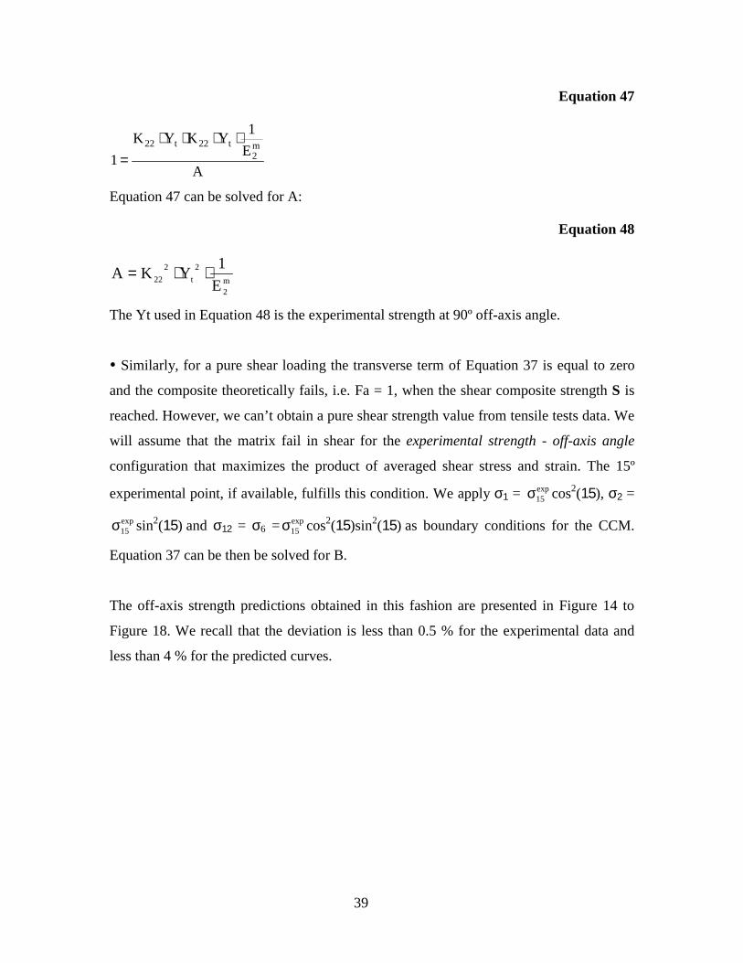
39
Equation 47
A
E
1YKYK
1m2
t22t22 ⋅⋅⋅⋅=
Equation 47 can be solved for A:
Equation 48
m2
2
t
2
22 E
1YKA ⋅⋅=
The Yt used in Equation 48 is the experimental strength at 90º off-axis angle.
é Similarly, for a pure shear loading the transverse term of Equation 37 is equal to zero
and the composite theoretically fails, i.e. Fa = 1, when the shear composite strength S is
reached. However, we can’t obtain a pure shear strength value from tensile tests data. We
will assume that the matrix fail in shear for the experimental strength - off-axis angle
configuration that maximizes the product of averaged shear stress and strain. The 15º
experimental point, if available, fulfills this condition. We apply σ1 = exp15σ cos2(15), σ2 =
exp15σ sin2(15) and σ12 = σ6 = exp
15σ cos2(15)sin2(15) as boundary conditions for the CCM.
Equation 37 can be then be solved for B.
The off-axis strength predictions obtained in this fashion are presented in Figure 14 to
Figure 18. We recall that the deviation is less than 0.5 % for the experimental data and
less than 4 % for the predicted curves.
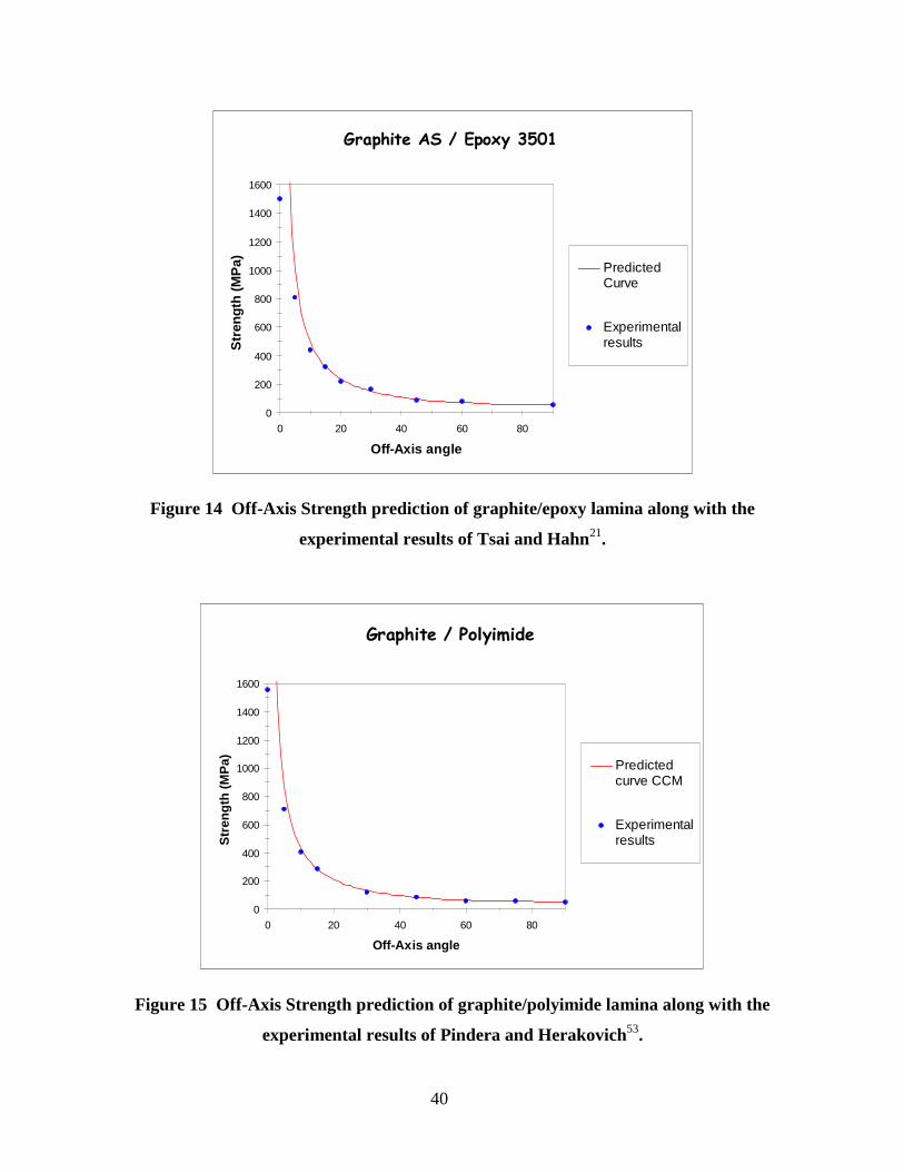
40
*UDSKLWH�$6���(SR[\�����
0
200
400
600
800
1000
1200
1400
1600
0 20 40 60 80
Off-Axis angle
Str
eng
th (
MP
a) PredictedCurve
Experimentalresults
Figure 14 Off-Axis Strength prediction of graphite/epoxy lamina along with the
experimental results of Tsai and Hahn21.
*UDSKLWH���3RO\LPLGH
0
200
400
600
800
1000
1200
1400
1600
0 20 40 60 80
Off-Axis angle
Str
eng
th (
MP
a) Predictedcurve CCM
Experimentalresults
Figure 15 Off-Axis Strength prediction of graphite/polyimide lamina along with the
experimental results of Pindera and Herakovich53.
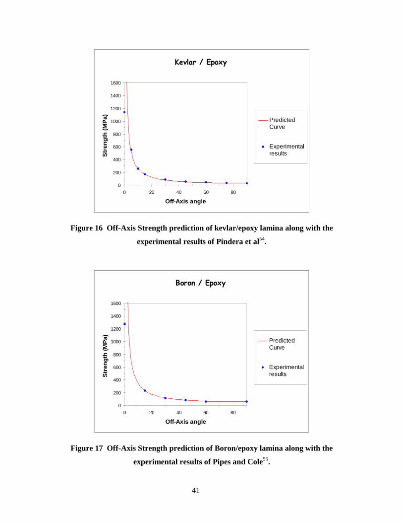
41
.HYODU���(SR[\
0
200
400
600
800
1000
1200
1400
1600
0 20 40 60 80
Off-Axis angle
Str
eng
th (
MP
a) PredictedCurve
Experimentalresults
Figure 16 Off-Axis Strength prediction of kevlar/epoxy lamina along with the
experimental results of Pindera et al54.
%RURQ���(SR[\
0
200
400
600
800
1000
1200
1400
1600
0 20 40 60 80
Off-Axis angle
Str
eng
th (
MP
a) PredictedCurve
Experimentalresults
Figure 17 Off-Axis Strength prediction of Boron/epoxy lamina along with the
experimental results of Pipes and Cole55.
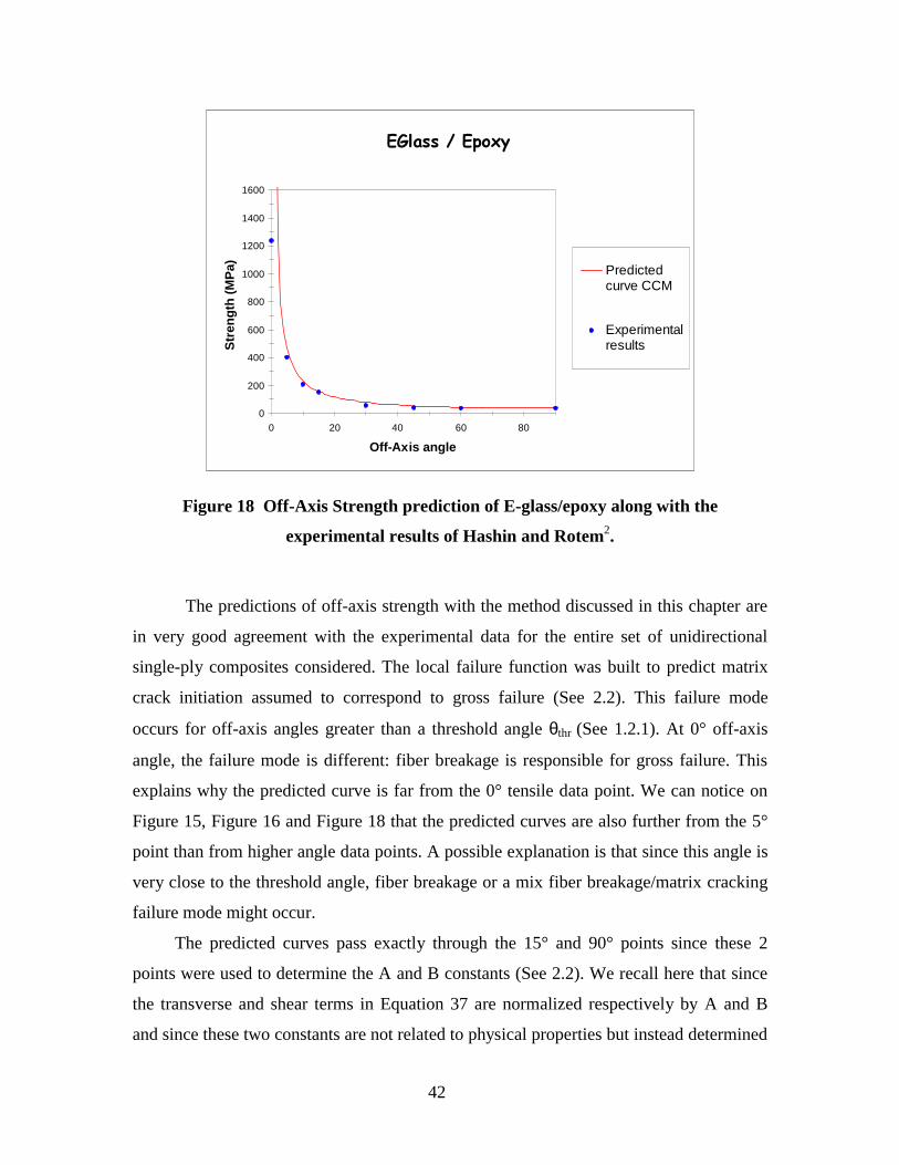
42
(*ODVV���(SR[\
0
200
400
600
800
1000
1200
1400
1600
0 20 40 60 80
Off-Axis angle
Str
eng
th (
MP
a) Predictedcurve CCM
Experimentalresults
Figure 18 Off-Axis Strength prediction of E-glass/epoxy along with the
experimental results of Hashin and Rotem2.
The predictions of off-axis strength with the method discussed in this chapter are
in very good agreement with the experimental data for the entire set of unidirectional
single-ply composites considered. The local failure function was built to predict matrix
crack initiation assumed to correspond to gross failure (See 2.2). This failure mode
occurs for off-axis angles greater than a threshold angle θthr (See 1.2.1). At 0° off-axis
angle, the failure mode is different: fiber breakage is responsible for gross failure. This
explains why the predicted curve is far from the 0° tensile data point. We can notice on
Figure 15, Figure 16 and Figure 18 that the predicted curves are also further from the 5°
point than from higher angle data points. A possible explanation is that since this angle is
very close to the threshold angle, fiber breakage or a mix fiber breakage/matrix cracking
failure mode might occur.
The predicted curves pass exactly through the 15° and 90° points since these 2
points were used to determine the A and B constants (See 2.2). We recall here that since
the transverse and shear terms in Equation 37 are normalized respectively by A and B
and since these two constants are not related to physical properties but instead determined
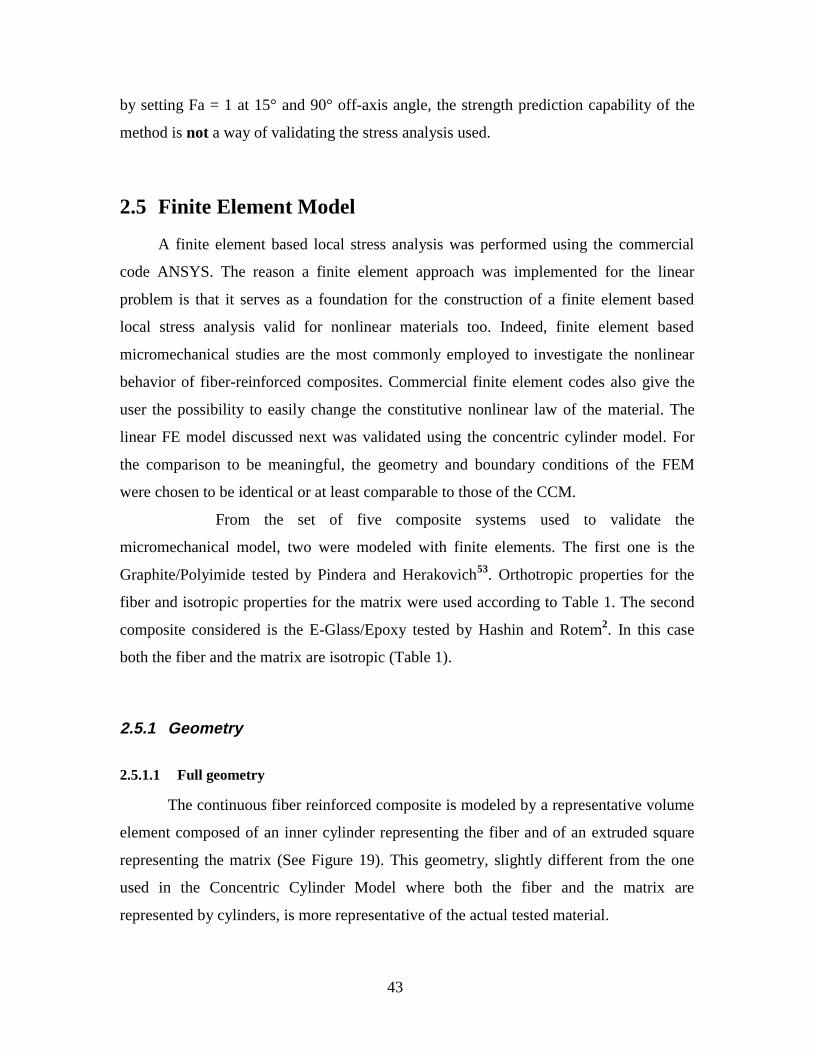
43
by setting Fa = 1 at 15° and 90° off-axis angle, the strength prediction capability of the
method is not a way of validating the stress analysis used.
2.5 Finite Element Model
A finite element based local stress analysis was performed using the commercial
code ANSYS. The reason a finite element approach was implemented for the linear
problem is that it serves as a foundation for the construction of a finite element based
local stress analysis valid for nonlinear materials too. Indeed, finite element based
micromechanical studies are the most commonly employed to investigate the nonlinear
behavior of fiber-reinforced composites. Commercial finite element codes also give the
user the possibility to easily change the constitutive nonlinear law of the material. The
linear FE model discussed next was validated using the concentric cylinder model. For
the comparison to be meaningful, the geometry and boundary conditions of the FEM
were chosen to be identical or at least comparable to those of the CCM.
From the set of five composite systems used to validate the
micromechanical model, two were modeled with finite elements. The first one is the
Graphite/Polyimide tested by Pindera and Herakovich53. Orthotropic properties for the
fiber and isotropic properties for the matrix were used according to Table 1. The second
composite considered is the E-Glass/Epoxy tested by Hashin and Rotem2. In this case
both the fiber and the matrix are isotropic (Table 1).
2.5.1 Geometry
2.5.1.1 Full geometry
The continuous fiber reinforced composite is modeled by a representative volume
element composed of an inner cylinder representing the fiber and of an extruded square
representing the matrix (See Figure 19). This geometry, slightly different from the one
used in the Concentric Cylinder Model where both the fiber and the matrix are
represented by cylinders, is more representative of the actual tested material.
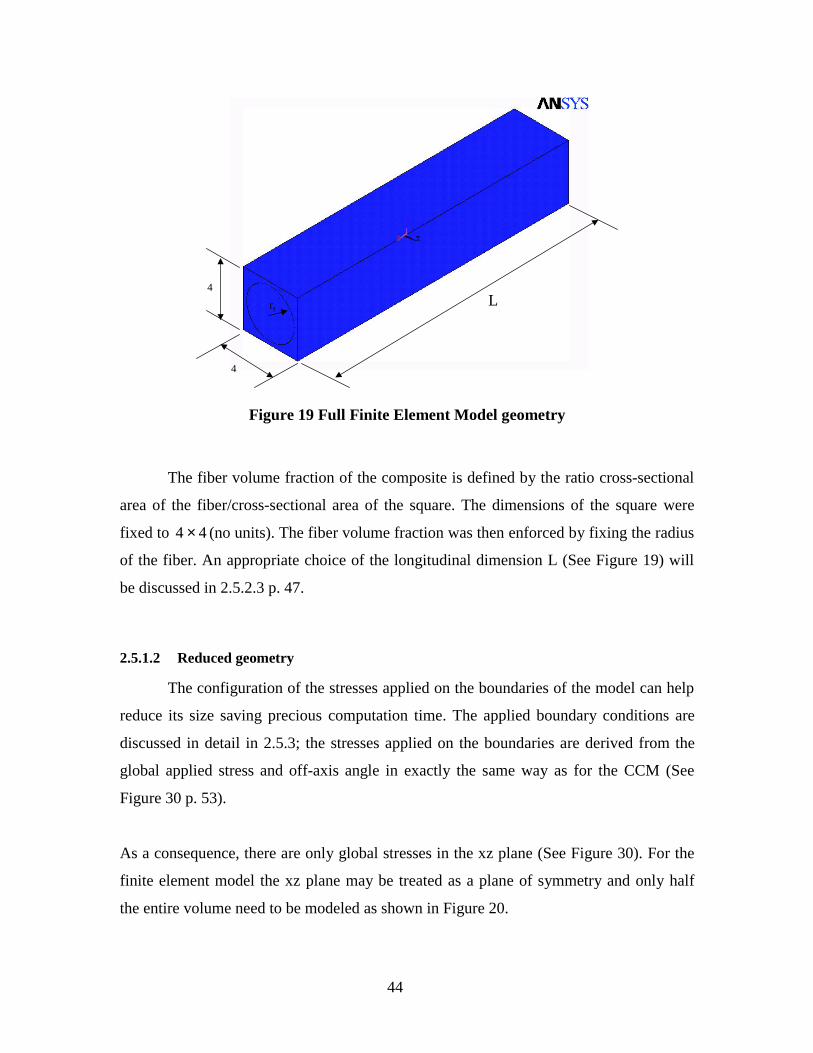
44
L
4
4
rf
Figure 19 Full Finite Element Model geometry
The fiber volume fraction of the composite is defined by the ratio cross-sectional
area of the fiber/cross-sectional area of the square. The dimensions of the square were
fixed to 4 4× (no units). The fiber volume fraction was then enforced by fixing the radius
of the fiber. An appropriate choice of the longitudinal dimension L (See Figure 19) will
be discussed in 2.5.2.3 p. 47.
2.5.1.2 Reduced geometry
The configuration of the stresses applied on the boundaries of the model can help
reduce its size saving precious computation time. The applied boundary conditions are
discussed in detail in 2.5.3; the stresses applied on the boundaries are derived from the
global applied stress and off-axis angle in exactly the same way as for the CCM (See
Figure 30 p. 53).
As a consequence, there are only global stresses in the xz plane (See Figure 30). For the
finite element model the xz plane may be treated as a plane of symmetry and only half
the entire volume need to be modeled as shown in Figure 20.
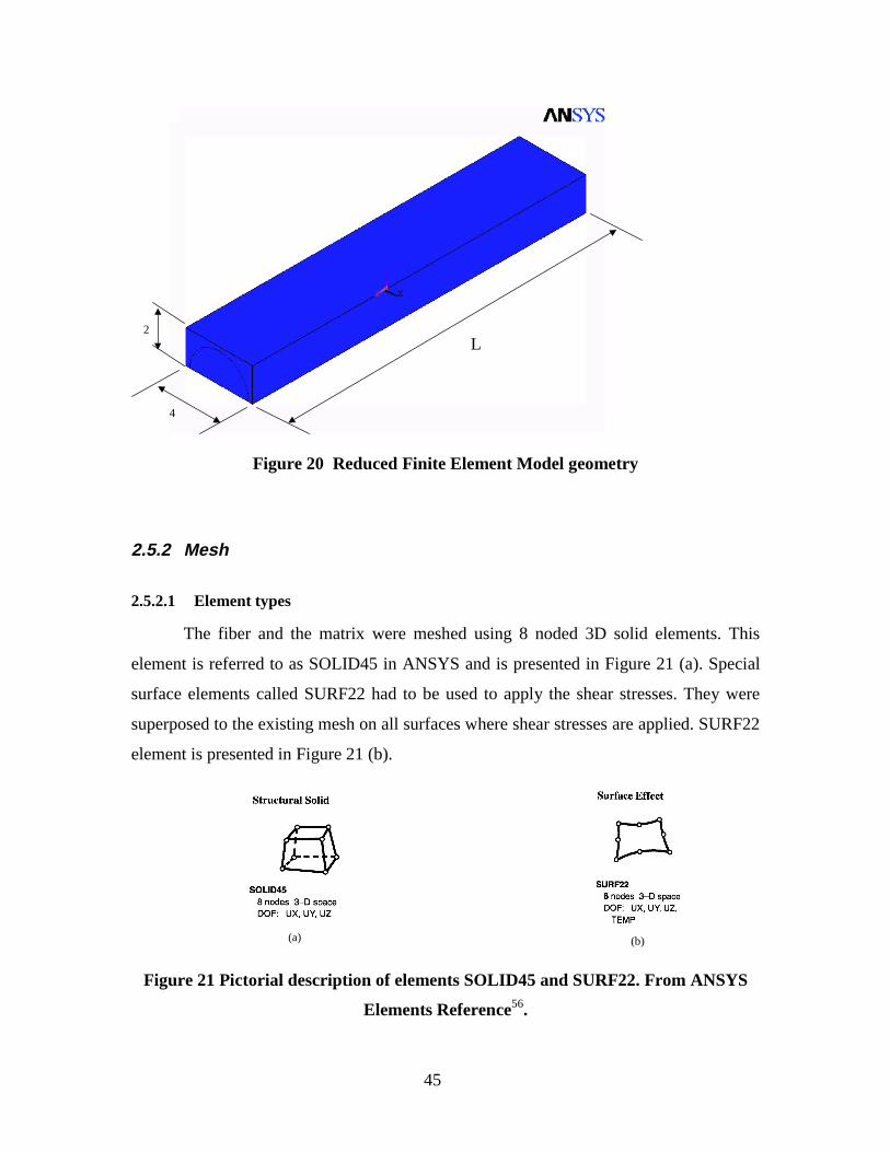
45
L
4
2
Figure 20 Reduced Finite Element Model geometry
2.5.2 Mesh
2.5.2.1 Element types
The fiber and the matrix were meshed using 8 noded 3D solid elements. This
element is referred to as SOLID45 in ANSYS and is presented in Figure 21 (a). Special
surface elements called SURF22 had to be used to apply the shear stresses. They were
superposed to the existing mesh on all surfaces where shear stresses are applied. SURF22
element is presented in Figure 21 (b).
(a) (b)
Figure 21 Pictorial description of elements SOLID45 and SURF22. From ANSYS
Elements Reference56.
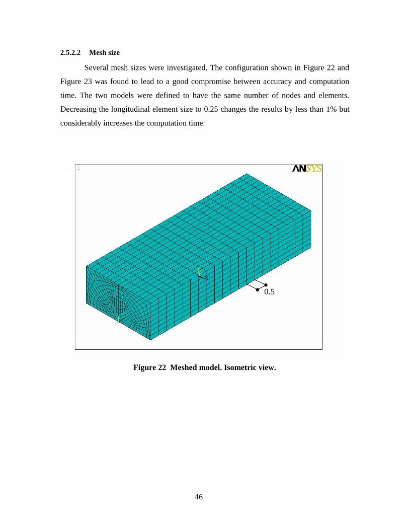
46
2.5.2.2 Mesh size
Several mesh sizes were investigated. The configuration shown in Figure 22 and
Figure 23 was found to lead to a good compromise between accuracy and computation
time. The two models were defined to have the same number of nodes and elements.
Decreasing the longitudinal element size to 0.25 changes the results by less than 1% but
considerably increases the computation time.
0.5
Figure 22 Meshed model. Isometric view.
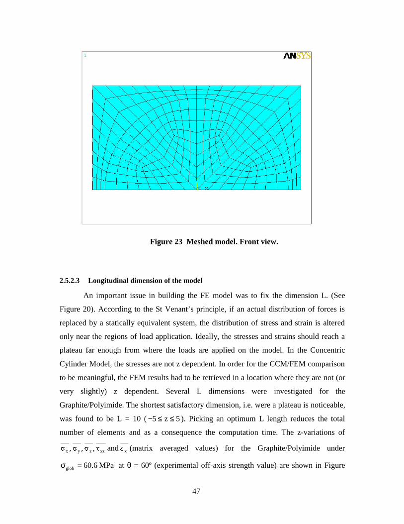
47
Figure 23 Meshed model. Front view.
2.5.2.3 Longitudinal dimension of the model
An important issue in building the FE model was to fix the dimension L. (See
Figure 20). According to the St Venant’s principle, if an actual distribution of forces is
replaced by a statically equivalent system, the distribution of stress and strain is altered
only near the regions of load application. Ideally, the stresses and strains should reach a
plateau far enough from where the loads are applied on the model. In the Concentric
Cylinder Model, the stresses are not z dependent. In order for the CCM/FEM comparison
to be meaningful, the FEM results had to be retrieved in a location where they are not (or
very slightly) z dependent. Several L dimensions were investigated for the
Graphite/Polyimide. The shortest satisfactory dimension, i.e. were a plateau is noticeable,
was found to be L = 10 (− ≤ ≤5 5z ). Picking an optimum L length reduces the total
number of elements and as a consequence the computation time. The z-variations of
xxzzyx and , , , (matrix averaged values) for the Graphite/Polyimide under
MPa 6.60glob =σ at θ = 60º (experimental off-axis strength value) are shown in Figure
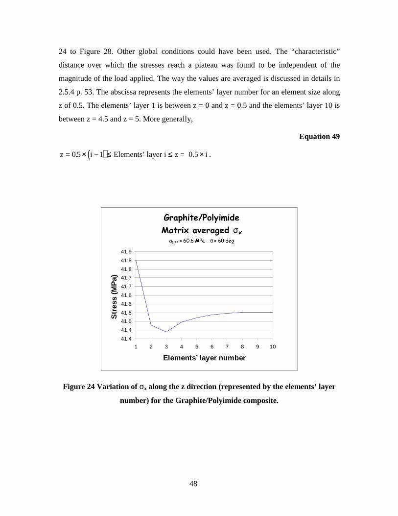
48
24 to Figure 28. Other global conditions could have been used. The “characteristic”
distance over which the stresses reach a plateau was found to be independent of the
magnitude of the load applied. The way the values are averaged is discussed in details in
2.5.4 p. 53. The abscissa represents the elements’ layer number for an element size along
z of 0.5. The elements’ layer 1 is between z = 0 and z = 0.5 and the elements’ layer 10 is
between z = 4.5 and z = 5. More generally,
Equation 49
( )z i Elements= × − ≤ ≤ ×0 5 1. ’ layer i z = 0.5 i .
*UDSKLWH�3RO\LPLGH0DWUL[�DYHUDJHG�σ[
σJORE� ������03D����θ� ����GHJ
41.4
41.4
41.5
41.5
41.6
41.6
41.7
41.7
41.8
41.8
41.9
1 2 3 4 5 6 7 8 9 10
Elements’ layer number
Str
ess
(MP
a)
Figure 24 Variation of σx along the z direction (represented by the elements’ layer
number) for the Graphite/Polyimide composite.
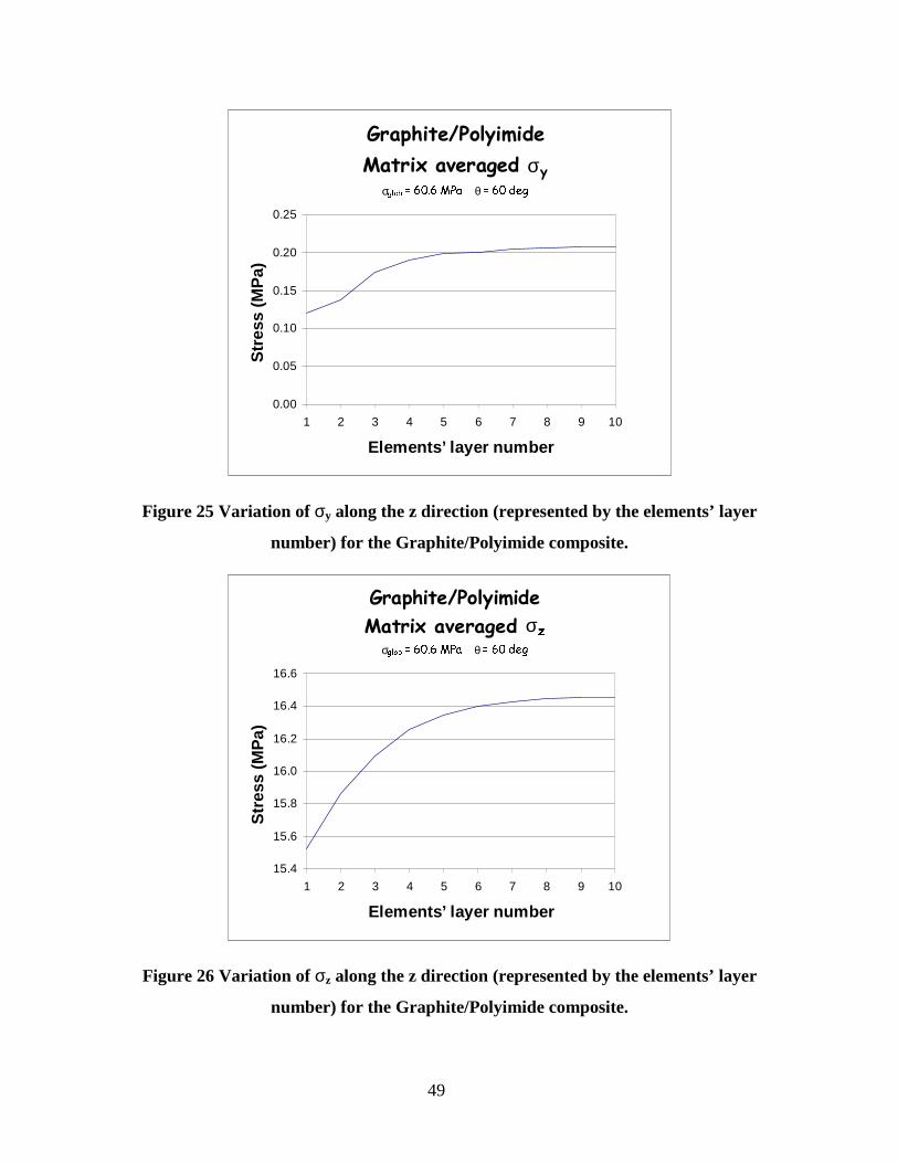
49
*UDSKLWH�3RO\LPLGH0DWUL[�DYHUDJHG�σ\
σJORE� ������03D����θ� ����GHJ
0.00
0.05
0.10
0.15
0.20
0.25
1 2 3 4 5 6 7 8 9 10
Elements’ layer number
Str
ess
(MP
a)
Figure 25 Variation of σy along the z direction (represented by the elements’ layer
number) for the Graphite/Polyimide composite.
*UDSKLWH�3RO\LPLGH0DWUL[�DYHUDJHG�σ]
σJORE� ������03D����θ� ����GHJ
15.4
15.6
15.8
16.0
16.2
16.4
16.6
1 2 3 4 5 6 7 8 9 10
Elements’ layer number
Str
ess
(MP
a)
Figure 26 Variation of σz along the z direction (represented by the elements’ layer
number) for the Graphite/Polyimide composite.
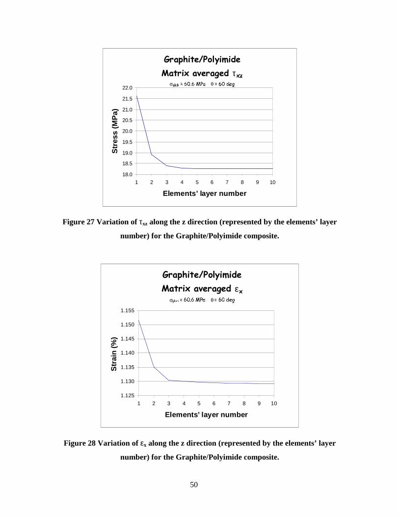
50
*UDSKLWH�3RO\LPLGH0DWUL[�DYHUDJHG�τ[]
σJORE� ������03D����θ� ����GHJ
18.0
18.5
19.0
19.5
20.0
20.5
21.0
21.5
22.0
1 2 3 4 5 6 7 8 9 10
Elements’ layer number
Str
ess
(MP
a)
Figure 27 Variation of τxz along the z direction (represented by the elements’ layer
number) for the Graphite/Polyimide composite.
*UDSKLWH�3RO\LPLGH0DWUL[�DYHUDJHG�ε[
σJORE� ������03D����θ� ����GHJ
1.125
1.130
1.135
1.140
1.145
1.150
1.155
1 2 3 4 5 6 7 8 9 10
Elements’ layer number
Str
ain
(%
)
Figure 28 Variation of εx along the z direction (represented by the elements’ layer
number) for the Graphite/Polyimide composite.

51
The same longitudinal length was adopted for the modeling of the E-Glass/Epoxy
composite. The number of elements, the number of nodes and the average run time for
the composites investigated are given in Table 3 for information.
Table 3 Finite Element Models information
Graphite/Epoxy and E-Glass/Epoxy
Number of SOLID45 elements 5760
Number of SURF22 elements 896
Total number of elements 6656
Total number of nodes 6636
Average run time 5 min. 20s
2.5.3 Boundary conditions
Displacement symmetry condition is applied on the xz bottom surface of the
reduced model and five nodes are pinned to prevent rigid body motions (See Figure 29).
The node referenced A in Figure 29 is pinned in all directions to prevent translations in
the 3 directions. Nodes B and C are pinned in the x direction and nodes D and E in the z
direction to prevent rotation of the entire structure around the y-axis. Rotation around the
x and z-axes are prevented through the symmetry condition on the xz bottom surface.
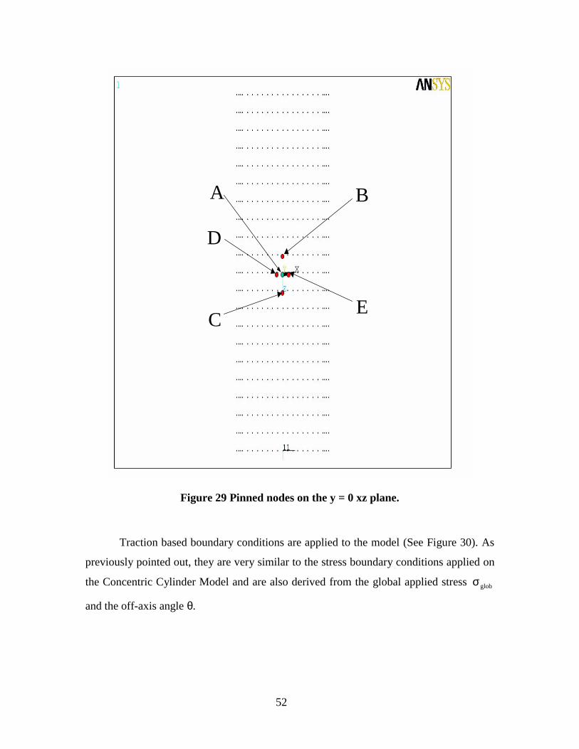
52
A B
C
D
E
Figure 29 Pinned nodes on the y = 0 xz plane.
Traction based boundary conditions are applied to the model (See Figure 30). As
previously pointed out, they are very similar to the stress boundary conditions applied on
the Concentric Cylinder Model and are also derived from the global applied stress σglob
and the off-axis angle θ.
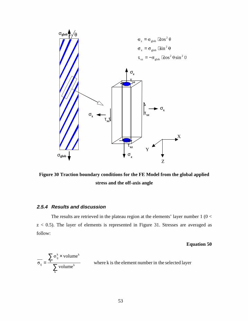
53
σglob
σx
z
σxτxz
σz
τxz
τxz
σ
τxz
X
Z
Y
θ
σglob
sincos
sin
cos
22globxz
2globx
2globz
⋅−=
⋅=
⋅=
Figure 30 Traction boundary conditions for the FE Model from the global applied
stress and the off-axis angle
2.5.4 Results and discussion
The results are retrieved in the plateau region at the elements’ layer number 1 (0 <
z < 0.5). The layer of elements is represented in Figure 31. Stresses are averaged as
follow:
Equation 50
layer selected in thenumber element theisk where volume
volume
k
kk
kkij
ij ∑∑ ×
=
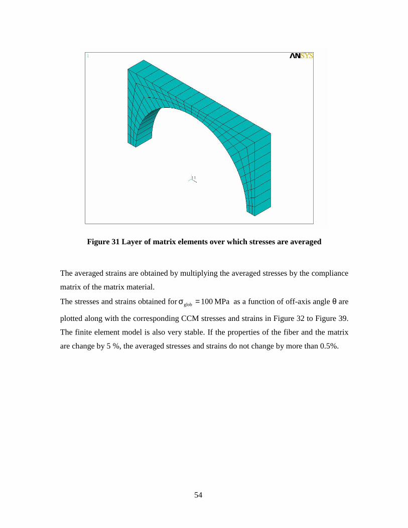
54
Figure 31 Layer of matrix elements over which stresses are averaged
The averaged strains are obtained by multiplying the averaged stresses by the compliance
matrix of the matrix material.
The stresses and strains obtained for MPa 100glob =σ as a function of off-axis angle θ are
plotted along with the corresponding CCM stresses and strains in Figure 32 to Figure 39.
The finite element model is also very stable. If the properties of the fiber and the matrix
are change by 5 %, the averaged stresses and strains do not change by more than 0.5%.
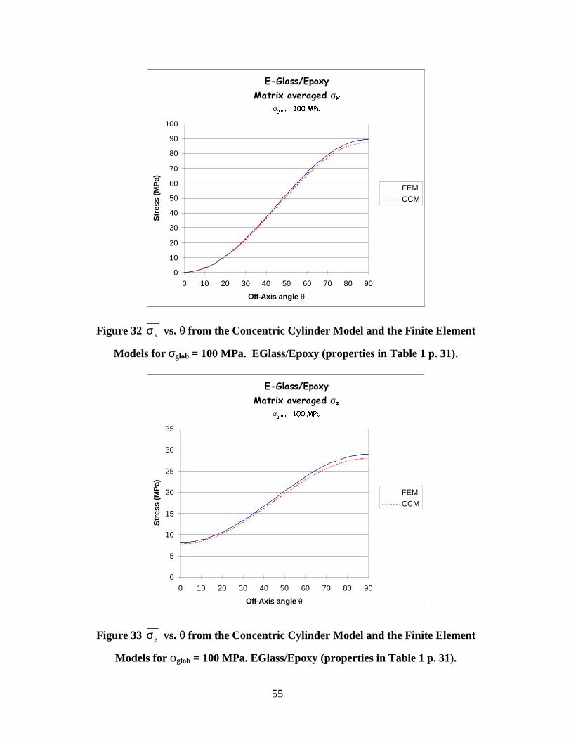
55
(�*ODVV�(SR[\0DWUL[�DYHUDJHG�σ[
σJORE� �����03D
0
10
20
30
40
50
60
70
80
90
100
0 10 20 30 40 50 60 70 80 90
Off-Axis angle θ
Str
ess
(MP
a)
FEM
CCM
Figure 32 xσ vs. θ from the Concentric Cylinder Model and the Finite Element
Models for σglob = 100 MPa. EGlass/Epoxy (properties in Table 1 p. 31).
(�*ODVV�(SR[\0DWUL[�DYHUDJHG�σ]
σJORE� �����03D
0
5
10
15
20
25
30
35
0 10 20 30 40 50 60 70 80 90
Off-Axis angle θ
Str
ess
(MP
a)
FEM
CCM
Figure 33 zσ vs. θ from the Concentric Cylinder Model and the Finite Element
Models for σglob = 100 MPa. EGlass/Epoxy (properties in Table 1 p. 31).
56
(�*ODVV�(SR[\0DWUL[�DYHUDJHG�τ[]
σJORE� �����03D
-40
-35
-30
-25
-20
-15
-10
-5
00 10 20 30 40 50 60 70 80 90
Off-Axis angle θ
Str
ess
(MP
a)
FEM
CCM
Figure 34 xzτ vs. θ from the Concentric Cylinder Model and the Finite Element
Models for σglob = 100 MPa. EGlass/Epoxy (properties in Table 1 p. 31).
(�*ODVV�(SR[\0DWUL[�DYHUDJHG�ε[
σJORE� �����03D
-0.5
0.0
0.5
1.0
1.5
2.0
2.5
0 10 20 30 40 50 60 70 80 90
Off-Axis angle θ
Str
ain
(%
)
FEM
CCM
Figure 35 xε vs. θ from the Concentric Cylinder Model and the Finite Element
Models for σglob = 100 MPa. EGlass/Epoxy (properties in Table 1 p. 31).
57
*UDSKLWH�3RO\LPLGH0DWUL[�DYHUDJHG�σ[
σJORE� �����03D
0
10
20
30
40
50
60
70
80
90
100
0 10 20 30 40 50 60 70 80 90
Off-Axis angle θ
Str
ess
(MP
a)
FEM
CCM
Figure 36 xσ vs. θ from the Concentric Cylinder Model and the Finite Element
Models for σglob = 100 MPa. Graphite/Polyimide (properties in Table 1 p. 31).
*UDSKLWH�3RO\LPLGH0DWUL[�DYHUDJHG�σ]
σJORE� �����03D
0
5
10
15
20
25
30
35
40
0 10 20 30 40 50 60 70 80 90
Off-Axis angle θ
Str
ess
(MP
a)
FEM
CCM
Figure 37 zσ vs. θ from the Concentric Cylinder Model and the Finite Element
Models for σglob = 100 MPa. Graphite/Polyimide (properties in Table 1 p. 31).

58
*UDSKLWH�3RO\LPLGH0DWUL[�DYHUDJHG�τ[]
σJORE� �����03D
-40
-35
-30
-25
-20
-15
-10
-5
00 10 20 30 40 50 60 70 80 90
Off-Axis angle θ
Str
ess
(MP
a)
FEM
CCM
Figure 38 xzτ vs. θ from the Concentric Cylinder Model and the Finite Element
Models for σglob = 100 MPa. Graphite/Polyimide (properties in Table 1 p. 31).
*UDSKLWH�3RO\LPLGH0DWUL[�DYHUDJHG�ε[
σJORE� �����03D
-0.5
0.0
0.5
1.0
1.5
2.0
2.5
3.0
0 10 20 30 40 50 60 70 80 90
Off-Axis angle θ
Str
ain
(%
)
FEM
CCM
Figure 39 xε vs. θ from the Concentric Cylinder Model and the Finite Element
Models for σglob = 100 MPa. Graphite/Polyimide (properties in Table 1 p. 31).
59
The obtained values of stresses and strains are in good agreement with the CCM
results. The difference between the two models is slightly larger in the case of the
Graphite/Polyimide. For both composites, the maximum CCM/FEM difference is found
for τ xz at 45°. It doesn’t exceed 8%. All the other stress and strain values match within
less than 3%.
60
CHAPTER 3 AN OFF-AXIS STRENGTH PREDICTION
APPROACH FOR RUBBER BASED UNIDIRECTIONAL
COMPOSITES
3.1 Introduction
The failure function used in CHAPTER 2 was constructed to eventually capture
the nonlinear behavior of the material where it is applied. To check this feature, an
attempt was made to predict off-axis strength for a steel-cord/rubber unidirectional
composite using the failure function. The rubbery matrix is indeed expected to be
nonlinear. The challenge here lies in constructing a local stress analysis with nonlinear
capabilities. A finite element stress analysis based on the FE model constructed in
CHAPTER 2 was considered. This nonlinear FE analysis is still under development.
Divergence problems were encountered in the solution process. These problems along
with possible solutions are discussed in detail in 3.3 p. 77. The general methodology that
we planned to use is also discussed in this section.
Rubber based materials often follow an hyperelastic law (See 1.2.4 p. 16). The
stress/strain behavior of the rubber used in the steel-cord/rubber composite considered
was determined from experimental static tensile tests on dogbone specimens. To generate
experimental off-axis strength data, the composite laminae and two plies laminates were
tested in static tensile tests for different cord orientations. To obtain the instantaneous
elastic response of the material, the rate of loading was high (high enough for relaxation
and viscoelastic behaviors not to occur).
3.2 Experimental work
3.2.1 Materials
In order to protect proprietary information, the source and composition of the
materials tested in this work will not be described. The geometry and dimensions

61
(including gage length) of the different specimens are presented in Figure 40 to Figure
42.
3.2.1.1 Rubber dogbone specimens
Gage length = 20 mm
45 mm
Thickness = 2 mm
2 mm
Figure 40 Dogbone Specimen
3.2.1.2 Off-axis unidirectional steel-cord/rubber laminae
25.4 mm
300.0 mm
Thickness = 2 mm
mm 200.0length Gage ≅
Figure 41 Unidirectional steel-cord/rubber lamina
Specimens with 15º, 18º, 30º, 45º, 60º and 90º off-axis angle (angle between the
steel cord direction and the loading direction) were tested. The steel cords are brass
coated to ensure a good bonding with the rubber.
62
3.2.1.3 +30º/-30º and +18º/-18º steel-cord/rubber laminates
The total length and gage length of the laminates are the same as those of the
laminae. However, the thickness is twice that of the laminae, i.e. 4 mm. A side view is
shown Figure 42.
4 mm
Figure 42 Side view of +30º/-30º steel-cord/rubber specimen
3.2.2 Description of the experiments
Quasi-static tensile tests were performed on an “Instron” machine (See Figure
43) at room temperature. The load cells used for the laminae and laminates were
respectively 5 kN and 10kN. The dogbone were tested using a 1000 N load cell and
pneumatic grips specially adapted to small samples. The tests were performed in
displacement control at a rate of 50 mm per minute. The data acquisition was 250 msec
for all the specimens. Because crosshead displacement could not be used to obtain
accurate strain data due to stiffening effects in the grips, an extensometer capable of
recording strains up to 1000% was used for the laminae and laminates. It was placed on
the center of the tested specimen. This extensometer could not be used for the dogbones
because of their small size. A 14% engineering strain amplification factor (also from a
confidential source) was used to account for the grip effects.
63
Figure 43 Instron™ machine
3.2.3 Experimental results and discussion
3.2.3.1 Tensile tests on the rubber dogbones
3.2.3.1.1 Engineering stress-strain curve
The engineering stress (Area Initial
Forceeng =σ ) - engineering strain (
LengthInitial
Lengtheng
∆=ε )
curve of the rubber is given in Figure 44.
64
5XEEHU�GRJERQH�VSHFLPHQ
0
2
4
6
8
10
12
14
16
18
0 1 2 3 4 5Engineering strain
En
gin
eeri
ng
str
ess
(MP
a)
Figure 44 Engineering stress/strain curve
After a small kink between 0 and 15% strain, the curve is very close to a straight line.
The kink is usually more pronounced for rubber materials. The strain at failure is close to
450% at a stress level of 17 MPa. A method to determine if a material follows a Mooney-
Rivlin model (See p.18) was presented by Finney and Kumar49. This method was used
here. For an incompressible Mooney-Rivlin material under uniaxial tension, the stress-
strain equation can be expressed as:
Equation 51
( ) )aCC(aa2S 01102 ⋅+⋅−⋅= −
where S is the engineering stress, a is the stretch ratio (Length Original
Length1
∆+ ) and C10 and
C01 come from Equation 19 p. 18. From Equation 51, a plot of ( )2aa2
S −−⋅ against a-1
will give a straight line if the material follows a Mooney-Rivlin model. The slope will
give C01 and the intercept C10.The plot obtained for the tested rubber is shown in Figure
65
45. It clearly indicates that the rubber specimen does not follow a Mooney-Rivlin law. An
alternative constitutive relation will have to be use in the Finite Element stress analysis.
5XEEHU�GRJERQH�VSHFLPHQ
0
5
10
15
20
25
30
35
40
45
0 0.2 0.4 0.6 0.8 1
1/a
(s/2
)(a-
a^-2
) (
MP
a)
Figure 45 Mooney-Rivlin based plot for the rubber
3.2.3.1.2 True stress-strain curve
The nonlinearity of the material is more obvious in Figure 46 where true stress
and true strain are plotted. We recall that:
Equation Set 52
( )engtrueengengtrue 1LnLength Original
Length1Ln and )(1
Area Current
Force ε+=
∆+=εε+⋅σ==σ
66
5XEEHU�GRJERQH�VSHFLPHQ
0
10
20
30
40
50
60
70
80
90
100
0 0.5 1 1.5 2
True strain
Tru
e st
ress
(M
Pa)
Figure 46 True stress/strain curve
The nonlinear structural behavior of the rubber is expected to be mainly due to material
non-linear behavior as opposed to geometric nonlinearities in testing the dogbone
specimen. A good way to show the presence of material nonlinearity is to plot the Second
Piola-Kirchoff stress vs. the Green-Lagrange strain in the direction of loading.
3.2.3.1.3 Second Piola-Kirchoff stress - Green-Lagrange strain curve
Second Piola-Kirchoff stress and Green-Lagrange strain tensors are used in large
deformation theory of continuum mechanics. The Green-Lagrange strain tensor is
formulated to disregard the geometric nonlinearity effects while accounting for actual
material stretching. In the direction of loading, it is calculated as follows:
Equation 53
2
22
GL Length Initial2
Length InitialLength
⋅−=ε
67
The thermodynamically conjugate stress tensor [ ]S~
, Second Piola-Kirchoff, does not have
any physical meaning. It was derived from the following relation:
Equation 54
[ ] [ ] [ ]1FT1FT1FJS
~ ⋅
−=
−⋅⋅
−⋅=
· j
iij X
xF
∂∂
= is the deformation gradient where x is the deformed coordinate and X is the
undeformed coordinate
· J = Det[F]
· [T] is the true stress tensor
· [σ] is the Cauchy or engineering stress tensor
[ ]S~
is calculated for the dogbone specimen. We consider the gage length of the dogbone
specimen and assume a uniform strain field. We also assume that the originally
rectangular shape of the gage region of the dogbone will remain rectangular as the
specimen deforms (See Figure 47).
2
3
deformed
undeformed
1
L1
L2
L3
l1
l2
l3
Figure 47 Deformation of the gage part of the rubber dogbone

68
Because of symmetry, the problem can be reduced to 1/8th of the original rectangle as
shown in Figure 48.
1
2
3
L1/2
L2/2
L3/2
Figure 48 Reduced geometry
We have
Equation Set 55
2
LX0
L
lX
2/L
2/lXx
2
LX0
L
lX
2/L
2/lXx
2
LX0
L
lX
2/L
2/lXx
33
3
33
3
333
22
2
22
2
222
11
1
11
1
111
≤≤=⋅=
≤≤=⋅=
≤≤=⋅=
For an incompressible material, the volume is constant, i.e.
Equation 56
321321 LLLlll ⋅⋅=⋅⋅
We assume that
Equation Set 57
2121 lkl and LkL ⋅=⋅=
69
Substituting Equation Set 57 into Equation 56 and solving for l2 we obtain:
Equation 58
23
32 L
l
Ll ⋅=
From Equation Set 57 and Equation 58, we get:
Equation 59
13
31 L
l
Ll =
Using Equation Set 55 and Equation 59 we have:
Equation 60
2
LX0
l
LXx 1
13
311 ≤≤=
Similarly,
Equation 61
2
LX0
l
LXx 1
23
322 ≤≤=
We can now form the [F] matrix:
Equation 62
[ ]
=
3
3
3
3
3
3
L
l00
0l
L0
00l
L
F

70
The only non-zero stress component is in the direction of the applied normal load. From
Equation 54 and Equation 62 we finally obtain:
Equation 63
333
333 l
LS~ σ⋅=
Figure 49 is a plot of the calculated Second Piola-Kirchoff stress vs. the corresponding
Green-Lagrange strain. It shows the presence of material nonlinearity since the obtained
curve is not a straight line,
5XEEHU�GRJERQH�VSHFLPHQ
0
2
4
6
8
10
12
14
16
18
0 2 4 6 8 10 12 14 16
Green-Lagrange strain
2nd
Pio
la-K
irch
off
Str
ess
(MP
a)
Figure 49 Second Piola-Kirchoff stress vs. Green-Lagrange strain
3.2.3.2 Tensile tests on the off-axis unidirectional steel-cord/rubber laminae
As expected, failure occurred within the rubber close to the steel/rubber interface
and along a direction parallel to the direction of the cords. The broken specimens are
shown in Figure 50.

71
15° 18 ° 30 ° 45 ° 60 ° 90 °
Figure 50 Broken off-axis unidirectional laminae
Three specimens for each off-axis angle were tested. The results were very consistent and
a representative curve for each angle is presented next.
72
���GHJ�RII�D[LV�DQJOH
0
5
10
15
20
25
30
0 0.5 1 1.5 2
from X-headfrom extensometer
εeng
σ eng
(M
Pa)
Figure 51 Stress/strain curve for the 15º off-axis lamina
���GHJ�RII�D[LV�DQJOH
0
5
10
15
20
25
30
0 0.5 1 1.5 2
from X-headfrom extensometer
εeng
σ eng
(M
Pa)
Figure 52 Stress/strain curve for the 18º off-axis lamina
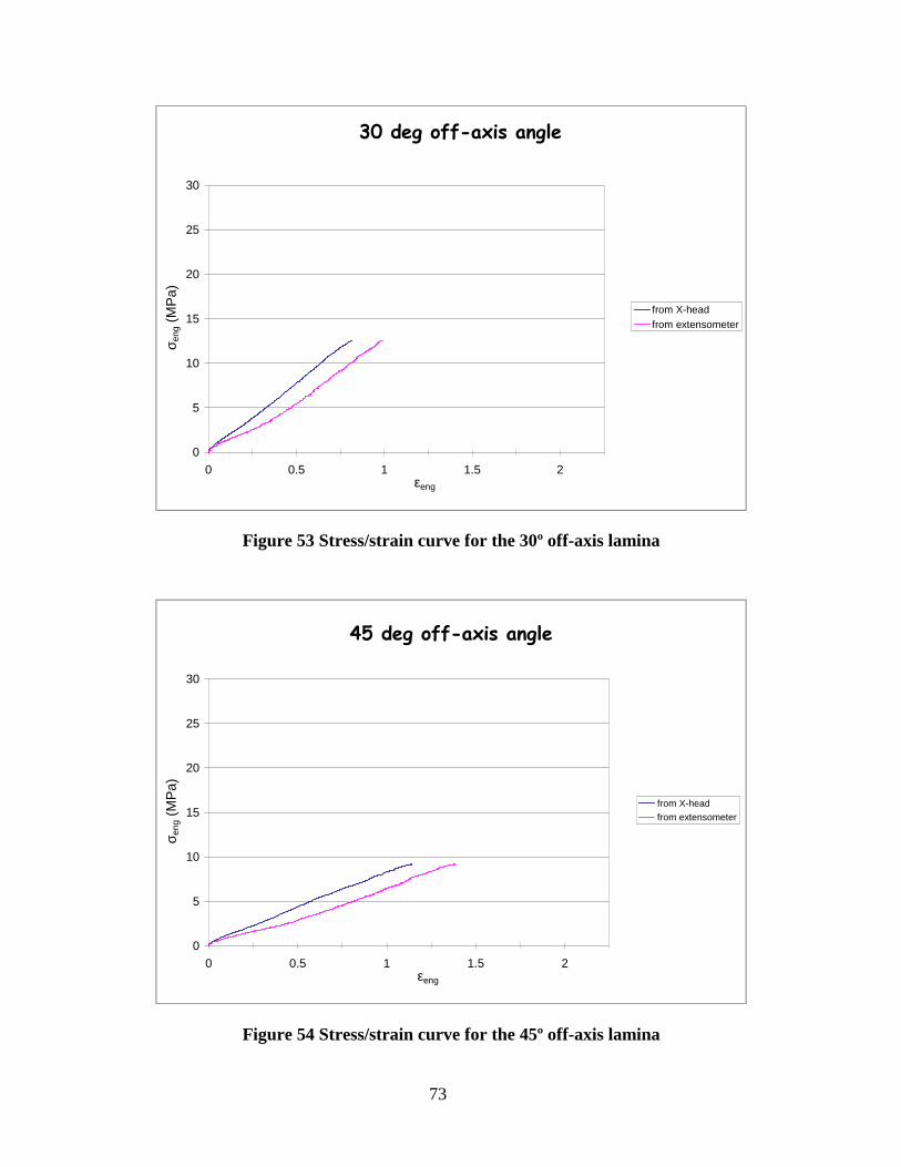
73
���GHJ�RII�D[LV�DQJOH
0
5
10
15
20
25
30
0 0.5 1 1.5 2
from X-headfrom extensometer
εeng
σ eng
(M
Pa)
Figure 53 Stress/strain curve for the 30º off-axis lamina
���GHJ�RII�D[LV�DQJOH
0
5
10
15
20
25
30
0 0.5 1 1.5 2
from X-head
from extensometer
εeng
σ eng
(M
Pa)
Figure 54 Stress/strain curve for the 45º off-axis lamina
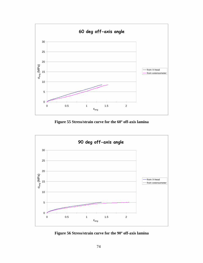
74
���GHJ�RII�D[LV�DQJOH
0
5
10
15
20
25
30
0 0.5 1 1.5 2
from X-headfrom extensometer
εeng
σ eng
(M
Pa)
Figure 55 Stress/strain curve for the 60º off-axis lamina
���GHJ�RII�D[LV�DQJOH
0
5
10
15
20
25
30
0 0.5 1 1.5 2
from X-headfrom extensometer
εeng
σ eng
(M
Pa)
Figure 56 Stress/strain curve for the 90º off-axis lamina

75
As the off-axis angle increases the contribution of the rubber phase on the overall
response of the composite increases and the nonlinear tendency of the stress-strain curve
is more pronounced. The larger slope of the curves obtained from crosshead displacement
compared to the ones obtained with the extensometer clearly show the stiffening effect of
the grips.
The early part of the 18º curve and the kink at 120% strain of the 90º curve are due to
testing problems and do not represent any actual physical trend or phenomenon.
3.2.3.3 Tensile tests on the off-axis unidirectional steel-cord/rubber laminates
Coalescence of matrix cracks along the fiber in each lamina leads to the V-shape
type of failure shown in Figure 57.
Figure 57 Broken +30º/-30º unidirectional laminate
The stress-strain curves of the +18º/-18º and +30º/-30º laminates are presented in Figure
58 and Figure 59.
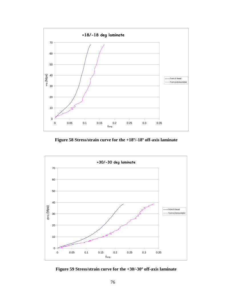
76
��������GHJ�ODPLQDWH�
0
10
20
30
40
50
60
70
0 0.05 0.1 0.15 0.2 0.25 0.3 0.35
from X-head
from extensometer
eng
(Mpa
)
εeng
Figure 58 Stress/strain curve for the +18º/-18º off-axis laminate
��������GHJ�ODPLQDWH
0
10
20
30
40
50
60
70
0 0.05 0.1 0.15 0.2 0.25 0.3 0.35
from X-head
from extensometer
εeng
σeng
(M
pa)
Figure 59 Stress/strain curve for the +30/-30º off-axis laminate
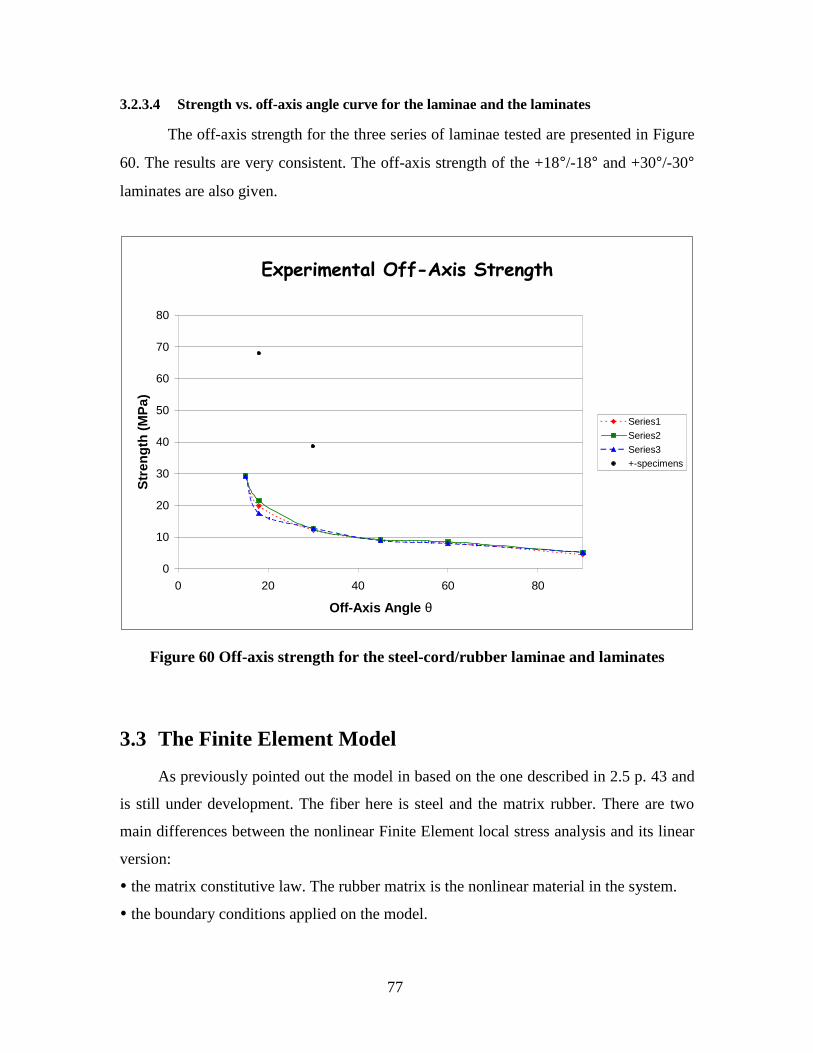
77
3.2.3.4 Strength vs. off-axis angle curve for the laminae and the laminates
The off-axis strength for the three series of laminae tested are presented in Figure
60. The results are very consistent. The off-axis strength of the +18°/-18° and +30°/-30°
laminates are also given.
([SHULPHQWDO�2II�$[LV�6WUHQJWK�
0
10
20
30
40
50
60
70
80
0 20 40 60 80
Off-Axis Angle θ
Str
eng
th (
MP
a)
Series1
Series2
Series3+-specimens
Figure 60 Off-axis strength for the steel-cord/rubber laminae and laminates
3.3 The Finite Element Model
As previously pointed out the model in based on the one described in 2.5 p. 43 and
is still under development. The fiber here is steel and the matrix rubber. There are two
main differences between the nonlinear Finite Element local stress analysis and its linear
version:
é the matrix constitutive law. The rubber matrix is the nonlinear material in the system.
é the boundary conditions applied on the model.
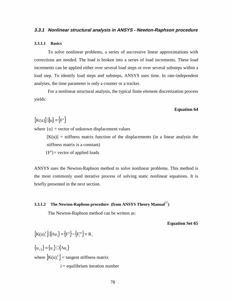
78
3.3.1 Nonlinear structural analysis in ANSYS - Newton-Raphson procedure
3.3.1.1 Basics
To solve nonlinear problems, a series of successive linear approximations with
corrections are needed. The load is broken into a series of load increments. These load
increments can be applied either over several load steps or over several substeps within a
load step. To identify load steps and substeps, ANSYS uses time. In rate-independent
analyses, the time parameter is only a counter or a tracker.
For a nonlinear structural analysis, the typical finite element discretization process
yields:
Equation 64
[ ] { } { }aFu)u(K =⋅
where {u} = vector of unknown displacement values
[K(u)] = stiffness matrix function of the displacements (in a linear analysis the
stiffness matrix is a constant)
{Fa}= vector of applied loads
ANSYS uses the Newton-Raphson method to solve nonlinear problems. This method is
the most commonly used iterative process of solving static nonlinear equations. It is
briefly presented in the next section.
3.3.1.2 The Newton-Raphson procedure (from ANSYS Theory Manual57)
The Newton-Raphson method can be written as:
Equation Set 65
[ ] { } { } { }
{ } { } { }ii1i
inri
ai
Ti
Xuu
RFFXK(u)
+=
=−=⋅
+
where [ ]TiK(u) = tangent stiffness matrix
i = equilibrium iteration number
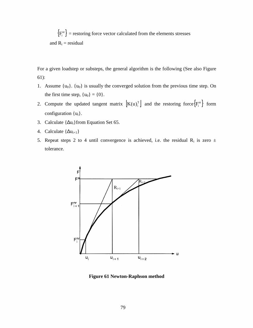
79
{ }nriF = restoring force vector calculated from the elements stresses
and Ri = residual
For a given loadstep or substeps, the general algorithm is the following (See also Figure
61):
1. Assume {u0}. {u0} is usually the converged solution from the previous time step. On
the first time step, {u0} = {0}.
2. Compute the updated tangent matrix [ ]Ti)u(K and the restoring force{ }nr
iF form
configuration {ui}.
3. Calculate {∆ui}from Equation Set 65.
4. Calculate {∆ui+1}
5. Repeat steps 2 to 4 until convergence is achieved, i.e. the residual Ri is zero ±
tolerance.
Ri+1
Ri+2
Figure 61 Newton-Raphson method

80
Different methods exist to help the Newton-Raphson algorithm to converge. For more
details the reader will refer to ANSYS Theory Manual57.
3.3.2 Rubber constitutive relation
We first planned to use 3D hyperelastic elements following a Mooney-Rivlin law.
Because of the experimental results showing the inadequacy of this type of constitutive
law, another approach was considered. The behavior of the rubber was entered in
ANSYS by discretizing the experimental stress-strain curve into small linear pieces.
Because of their large deformations and large strains capabilities the 3D structural
elements Solid45 (2.5.2.1 p. 45) were used, coupled with the user entered stress-strain
relation.
3.3.3 Stress or displacement boundary conditions ?
Stresses are easy to apply as boundary conditions because they can be directly
derived from the global applied stress (See Figure 30 p. 53). The derivation is valid for
linear materials as well as for non-linear materials. However, the ANSYS nonlinear
analysis does not converge when relatively high stresses are applied on the model. For
nonlinear analysis, displacement boundary conditions are known to give a more stable
model and to converge more easily. The problem is now to derive the displacements to
apply on the model from the global displacement in the direction of loading. In the case
of nonlinear materials unlike stresses, displacements can not be easily transformed from
one coordinate system to the other. A technique called Submodeling was used. It is
discussed in the next section.
3.3.4 Submodeling
The submodeling technique is used in finite element analysis to obtain more
accurate results in a region of the model. For our problem, ideally, the entire lamina
including all the steel-cords should be modeled and the results retrieved far from the free
edges and far from the region where the loads are applied. However, this type of
approach would be too computationally intense. An alternative is to consider the lamina
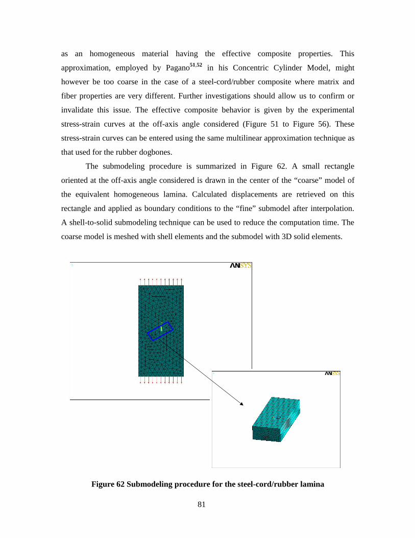
81
as an homogeneous material having the effective composite properties. This
approximation, employed by Pagano51,52 in his Concentric Cylinder Model, might
however be too coarse in the case of a steel-cord/rubber composite where matrix and
fiber properties are very different. Further investigations should allow us to confirm or
invalidate this issue. The effective composite behavior is given by the experimental
stress-strain curves at the off-axis angle considered (Figure 51 to Figure 56). These
stress-strain curves can be entered using the same multilinear approximation technique as
that used for the rubber dogbones.
The submodeling procedure is summarized in Figure 62. A small rectangle
oriented at the off-axis angle considered is drawn in the center of the “coarse” model of
the equivalent homogeneous lamina. Calculated displacements are retrieved on this
rectangle and applied as boundary conditions to the “fine” submodel after interpolation.
A shell-to-solid submodeling technique can be used to reduce the computation time. The
coarse model is meshed with shell elements and the submodel with 3D solid elements.
Figure 62 Submodeling procedure for the steel-cord/rubber lamina

82
CHAPTER 4 SUMMARY AND CONCLUSIONS
4.1 Summary
A new micromechanics-based model for the off-axis strength prediction of
unidirectional linear elastic laminae has been established. It uses:
• An existing concentric cylinder model to obtain the stresses and strains at the
matrix and fiber level.
• A new local failure function written as a reduced and normalized strain energy
density function.
The feasibility of this approach has been demonstrated by applying the model to different
composite laminae and comparing the results with data from the literature.
The same type of approach will be used for nonlinear laminae and the method has been
outlined in CHAPTER 3. The challenge here lies in constructing a local stress analysis. A
finite element analysis is currently under development for this nonlinear problem. It is
similar to the linear finite element analysis approach described in the present work and
which was validated with the concentric cylinder model. The comparison of the CCM
and the FEM is possible because:
• Comparable geometry and boundary conditions were used
• Stresses and strains obtained from the CCM do not vary along the longitudinal
z direction and FEM results were retrieved in a region where they don’t vary
with z either.
Tensile tests were performed on steel-cord/rubber laminae and laminates and the
constitutive behavior of the nonlinear rubber matrix was investigated.
4.2 Future work
4.2.1 Linear analysis
The following represent suggestions for future work:
83
é When A and B are expressed with matrix strength, we have seen that the predicted off-
axis strength are not correct. If we multiply A and B by 0.3, we consistently obtain very
good predictions. Investigations on how to relate this factor of 0.3 to fiber volume
fraction and/or stiffness of the matrix and the fiber would be a challenging future
direction of research.
é Different critical element volumes could be investigated. If matrix strength and strain-
to-failure properties are used for A and B, the currently calculated averaged stresses and
strains are too low (the off-axis strength is overestimated). If we consider a smaller
volume where the high stresses are concentrated, we should get better predictions.
Ultimately, we could use the maximum stress and strain values in the numerator of the
failure function.
4.2.2 Nonlinear analysis
The nonlinear finite element model is currently under development. Possible
methods to deal with the convergence problems are:
é modify the time step and the nonlinear analysis options
é find a way to enter more information about how the rubber behaves in order to better
describe the complex state of stress and strain that the matrix undergoes.
é ultimately, try to run the model on finite element code with explicit formulation
(ABAQUS explicit for example).
84
REFERENCES
1 Aboudi, J. “Micromechanical Analysis of the Strength of Unidirectional Fiber
Composites”, Composite Science and Technology, 33, 1988, pp.79-96.2 Hashin, Z. and Rotem, A. “A Fatigue Failure Criterion for Fiber Reinforced Materials”,
Journal of Composite Materials, 7, January 1973, pp. 448-464.3 Rosen, B.W. and Dow, N.F. “Mechanics of Failure of Fibrous Composites”, Fracture,
VII, H. Liebowitz Ed. Academic Press, 1972.4 Subramanian, S., Reifsnider K.L. and Stinchcomb, W.W. “A Micromechanics Model
for the Prediction of Fatigue Characteristics of Off-Axis Unidirectional Laminates”,
Applied Composite Materials, 1, 1994, pp. 69-74.5 Rahman, S. and Pecknold, D.A., Micromechanics-Based Analysis of Fiber-reinforced
Laminated Composites, Report UILU-ENG-90-2012, Urbana-Champaign, September
1992.6 Crossman, F.W., Warren, Wang, A.S.D. and Law, G.E. “Initiation and Growth of
Transverse Cracks and Edge Delamination in Composite Materials Part 2 Experimental
Correlation”, Dept. of Mechanical Engineering and Mechanics, Dept. Report, Drexel
University, 1979.7 Bjeletich, J.G., Crossman, F.W. and Warren W.J. “The Influences of Stacking Sequence
on Failure Modes in Quasi-Isotropic Graphite Epoxy Laminates”, Failure Modes in
Composite IV, AIME, 1979.8 Masters, J.E. and Reifsnider, K.L. “An Investigation of Cumulative Damage
Developments in Quasi-Isotropic Graphite/Epoxy Laminates”, Damage in Composites
Materials, ASTM STP775, K.L. Reifsnider ed., American Society for Testing and
Materials, 1982, pp. 40-62.9 Sun, C.T. and Jen, K.C. “On the Effect of Matrix Cracks on Laminate Strength”,
Journal of Reinforced Plastics and Composites, 6, 1987, pp. 208-222.10 Huang, Y.S. and Yeoh, O.H. “Crack Initiation and Propagation in Model Cord-Rubber
Composites”, Rubber Chemistry and Technology, 62, 1989, pp. 709-731.
85
11 Lee, B.L. and Liu, D.S. “Cumulative Damage of Fiber Reinforced Elastomer
Composites under Fatigue Loading”, Journal of Composites Materials, 28, No.13, 1994,
pp. 1261-1286.12 Sun, C.T. and Zhou S.G. “Failure of Quasi-Isotropic Composite Laminates with Free
Edges”, Journal of Reinforced Plastics and Composites, 7, November 1988, pp. 515-557.13 Breidenbach, R.F. and Lake, G.J. “Mechanics of Fracture in Two-Ply Laminates”,
Rubber Chemistry and Technology, 1979, pp. 52-96.14 Breidenbach, R.F. and Lake, G.J. “Application of Fracture Mechanics to Rubber
Articles Including Tires”, Philosophical Trans. Royal Soc. London, A299-189.15 Jones, R.M., Mechanics of Composite Materials, Taylor & Francis, 1975.16 Nahas, M.V. “Survey of Failure and Post-Failure Theories of Laminated Fiber-
Reinforced Composites”, Journal of Composites Technology and Research, 8, 1986, pp.
138-153.17 Tsai, S.W. “A Survey of Macroscopic Failure Criteria for Composite Materials”,
Journal of Reinforced Plastics and Composites, 3, January 1984, pp. 40-62.18 Hashin, Z. “Failure Criteria for Unidirectional Fiber Composites”, Journal of Applied
Mechanics, 47, June 1980, pp. 329-334.19 Goldenblat, I.I. and Kopnov, V.A. “Strength of Glass-Reinforced Plastics in the
Complex Stress State”, Mekhanika Polimerov, 7, 1965, pp. 70.20 Tsai, S.W. and Wu E.M. “A General Theory of Strength for Anisotropic Materials”,
Journal of Composites Materials, 1971, pp. 58-80.21 Tsai, S.W. and Hahn, H.T., Introduction to Composite Materials, Technomic
Publishing Company, 1980.22 Hoffman, O. “The Brittle Strength of Orthotropic Materials”, Journal of Composite
Materials, 1, 1967, pp. 200-206.23 Tsai, S.W. “Strength Characteristics of Composite Materials”, NASA CR-224, 1965.24 Hill, R. “A Theory of the Yielding and Plastic Flow of Anisotropic Materials”,
Proceedings of the Royal Society, Series A, 193, 1948, pp. 281.25 Huang, Z.M. “Micromechanical Modeling of Fatigue Strength of Unidirectional
Fibrous Composites”, private communication, 1999.
86
26 Subramanian, S., Reifsnider K.L. and Stinchcomb, W.W. “A Micromechanics Model
for the Prediction of Static Strength of Off-Axis Unidirectional Laminates”, Applied
Composite Materials, 1, 1994, pp. 75-79.27 Aboudi, J., Mechanics of Composite Materials – A Unified Micromechanical
Approach, Elsevier, 1991.28 Adams, D.F. and Doner, D.R. “Transverse Normal Loading of a Unidirectional
Composite”, Journal of Composite Materials, 1, April 1967, pp. 152-164.29 Adams, D.F. and Crane, D.A. “Finite Element Micromechanical Analysis of a
Unidirectional Composite Including Longitudinal Shear Loading”, Composite Structures,
18, 1984, pp. 1153-1165.30 Achenbach, J.D. and Zhu, H. “Effect of Interphases on Micro and Macromechanical
Behavior of Hexagonal-Array Fiber Composites”, Journal of Applied Mechanics, 57,
1990, pp. 956-963.31 Chamis, C.C. and Sendeckyj, G.P. “Critique on Theories Predicting Thermoelastic
Properties of Fibrous Composites”, Journal of Composite Materials, 2, 1968, pp. 332-
358.32 Averill, B.C. and Carman G.P. “Analytical Modeling of Micromechanical Stress
Variation in Continuous Fiber-Reinforced Composites”, Local Mechanics Concepts for
Composite Systems, IUTAM Symposium Blacksburg/VA 1991, J.N. Reddy, K.L.
Reifsnider (Eds), pp. 27-61.33 Kobayashi, S. and Ishikawa, T. “Elastic Properties of Unidirectional Fiber-Reinforced
Composites”, Fukugo Zairyo Kenkyu (Composite Materials and Structures), 3, No. 3,
1974, pp.12-20.34 Ishikawa, T. and Kobayashi, S. “Elastic Properties of Unidirectional Fiber-Reinforced
Composites”, Fukugo Zairyo Kenkyu (Composite Materials and Structures), 3, No. 4,
1974, pp.23-31.35 Naik, R.A. and Crews, J.H., Jr. “Micromechanical Analysis of Fiber-Matrix Interface
Stresses Under Thermomechanical Loadings”, Composite Materials: Testing and Design
(Eleventh Volume), ASTM STP 1206, E.T. Camponeshi, Jr., Ed., American Society for
Testing and Materials, Philadelphia, 1993, pp.205-219.

87
36 Paley, M. and Aboudi, J. “Micromechanical Analysis of Composites by the
Generalized Cells Model”, Mechanics of Materials, 14, 1992, Elsevier, pp. 127-139.37 Rivlin, R.S. “Large Elastic Deformations of Isotropic Materials; IV: Further
Developments of the General Theory”, Philosophical Trans. Royal Soc. London, A241,
1948, pp. 379-397.38 Oden, J.T. , Finite Elements of Nonlinear Continua, McGraw-Hill, New York, 1972.39 Mooney, M. “A theory for large elastic deformation”, Journal of Applied Physic, 11,
1940, pp. 582-597.40 Gadala, M.S. “On the Use of Bubble Functions and Modified Invariants for the
Analysis of Hyperelastic and Rubber-like materials”, Constitutive Laws for Engineering
Materials, Ed. C.S. Desai et al., ASME Press, Proc. Third International Conf. On
Constitutive Laws, Tucson, Arizona, January 1991, pp. 101-105.41 Swanson, S.R. “A Constitutive Model for High Elongation Elastic Materials”, Journal
of Engineering Materials and Technology, ASME Trans., 107, 1984, pp. 110-114.42 Blatz, P.J. and Ko W.L., “Application of finite elastic theory to the deformation of
rubbery materials”, Transcripts of the Society of Rheology, 6, 1962, pp. 223.43 Hart-Smith, L.J. “Elasticity Parameters for Finite Deformations of Rubber-like
Materials” ZAMP, 17, 1966, pp. 608-625.44 Gadala, M.S. “Unified Numerical Treatment of Hyperelastic and Rubber-like
Constitutive Laws”, Communications in Applied Numerical Methods, 7, 1991, pp. 581-
587.45 Ogden, R.W.,Proc. R. Soc. London, A328, 1972, pp. 567.46 Peng, S.T.J., “Nonlinear Multiaxial Finite Deformation Investigation of Solids
Propellants”, AFRPL TR-85-036, 1985.47 Valanis, K.C. and Landel R.F., Journal of Applied Physic, 38, 1967, pp. 2997.48 Peng, S.T.J. and Landel, R.F., Journal of Applied Physic, 43, 1972, pp. 3064.49 Finney, R.H. and Kumar, A. “Development of Material Constants for Nonlinear Finite-
Element Analysis”, Rubber Chemistry and Technology, 61, 1987, pp. 879-891.50 Plumtree, A. and Cheng, G. “A Fatigue Criterion for Life Prediction of Off-Axis
Unidirectional Composites”, ECCM, pp. 105-110.

88
51 Pagano, N.J. and Tandon, G.P. “Elastic Response of Multidirectional Coated-Fiber
Composites”, Composites Science and Technology, 31, 1988, pp. 273-293.52 Pagano, N.J. and Tandon, G.P. “Thermo-elastic Model for Multidirectional Coated-
Fiber Composites: Traction Formulation”, Composites Science and Technology, 38,
1990, pp. 247-269.53 Pindera, M.-J. and Herakovich, C.T., An Endochronic Theory for Transversely
Isotropic Fibrous Composites, The NASA-Virginia Tech Composites Program, VPI-E-
81-27, NASA NCCI-15, October 1981.54 Pindera, M.-J., Gurdal, Z., Hidde, J.S. and Herakovich, C.T., Mechanical and Thermal
Characterization of Unidirectional Aramid/Epoxy CCMS-86-08, VPI-86-29, Virginia
Polytechnic Institute and State University, 1986.55 Pipes, R.B. and Cole, B.W. “On the Off-Axis Strength Test for Anisotropic Materials”,
Journal of Composite Materials, 7, 1973, pp. 246-256.56 ANSYS Elements Reference.000853, Ninth Edition, SAS IP Inc, 1997.57 ANSYS Theory Reference.000855, Eight Edition, SAS IP Inc, 1997.
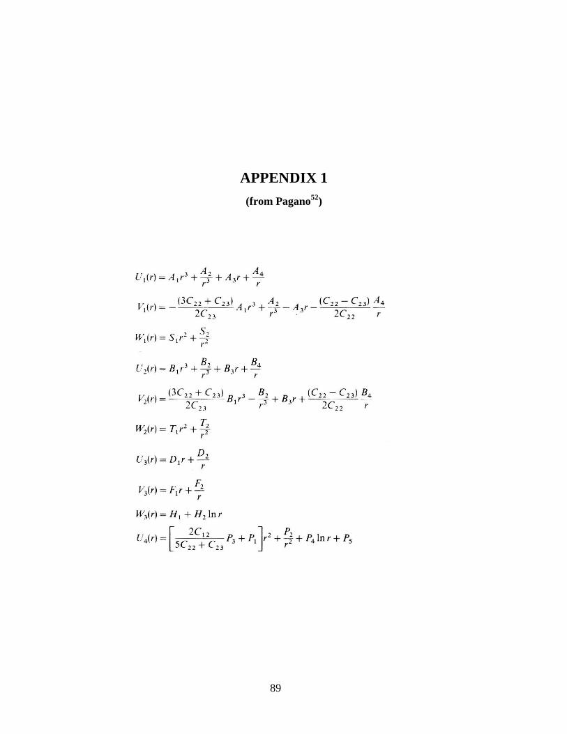
89
APPENDIX 1
(from Pagano52)
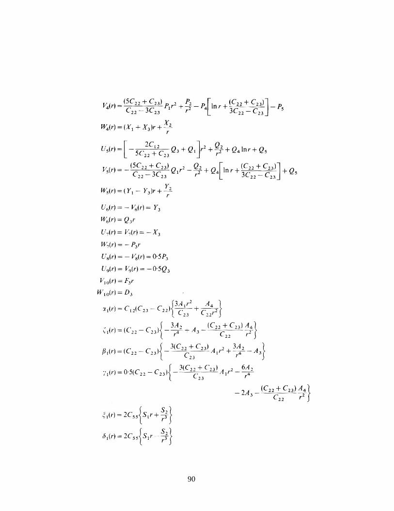
90
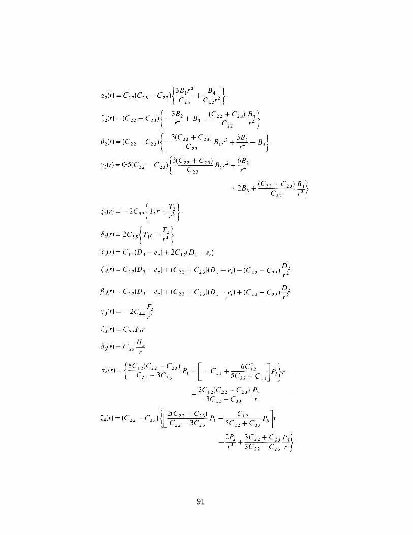
91
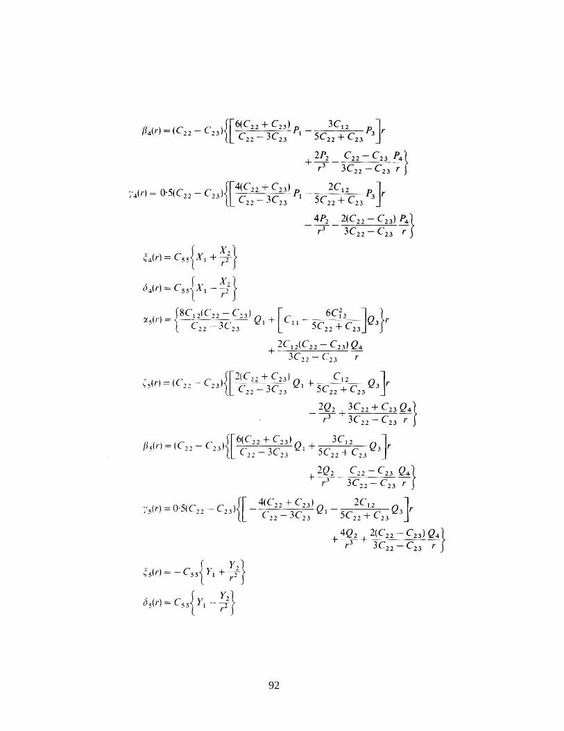
92
93
VITA
Jérémy Duthoit, son of Liliane Oter and Bruno Duthoit, was born on February 29,
1976 in Béthune, France. He grew up in Beuvry in the north of France. After obtaining
his Baccalauréat in Mathematics and Physics in 1993 at the Lycée Louis Blaringhem in
Béthune, France, Mr. Duthoit was admitted in the Université de Technologie de
Compiègne (UTC, France). After two years of general engineering, he entered the
department of Mechanical Engineering and specialized in Materials and Technologic
Innovation. He was then selected for an exchange program between UTC and Virginia
Tech. In August 1997, he moved to Blacksburg, Virginia, USA to enroll in the Master’s
Program of the Department of Materials Science and Engineering. He joined the
Materials Response Group where he conducted his research on mechanics of composites.
Jeremy intends to continue his work in the field of composite materials in academia or in
industries.
Jérémy Duthoit