A Methodology to Identify Alternative Suitable NoSQL Data ...

Air Force Institute of Technology Air Force Institute of Technology

AFIT Scholar AFIT Scholar

Theses and Dissertations Student Graduate Works

9-2020

A Methodology to Identify Alternative Suitable NoSQL Data A Methodology to Identify Alternative Suitable NoSQL Data

Models via Observation of Relational Database Interactions Models via Observation of Relational Database Interactions

Paul M. Beach

Follow this and additional works at: https://scholar.afit.edu/etd

Part of the Databases and Information Systems Commons

Recommended Citation Recommended Citation Beach, Paul M., "A Methodology to Identify Alternative Suitable NoSQL Data Models via Observation of Relational Database Interactions" (2020). Theses and Dissertations. 4339. https://scholar.afit.edu/etd/4339

This Dissertation is brought to you for free and open access by the Student Graduate Works at AFIT Scholar. It has been accepted for inclusion in Theses and Dissertations by an authorized administrator of AFIT Scholar. For more information, please contact [email protected].

https://scholar.afit.edu/

https://scholar.afit.edu/etd

https://scholar.afit.edu/graduate_works

https://scholar.afit.edu/etd?utm_source=scholar.afit.edu%2Fetd%2F4339&utm_medium=PDF&utm_campaign=PDFCoverPages

http://network.bepress.com/hgg/discipline/145?utm_source=scholar.afit.edu%2Fetd%2F4339&utm_medium=PDF&utm_campaign=PDFCoverPages

https://scholar.afit.edu/etd/4339?utm_source=scholar.afit.edu%2Fetd%2F4339&utm_medium=PDF&utm_campaign=PDFCoverPages

mailto:[email protected]

A Methodology to Identify Alternative SuitableNoSQL Data Models via Observation of

Relational Database Interactions

DISSERTATION

Paul M. Beach, Major, USAF

AFIT-ENV-DS-20-S-056

DEPARTMENT OF THE AIR FORCEAIR UNIVERSITY

AIR FORCE INSTITUTE OF TECHNOLOGY

Wright-Patterson Air Force Base, Ohio

DISTRIBUTION STATEMENT AAPPROVED FOR PUBLIC RELEASE; DISTRIBUTION UNLIMITED.

The views expressed in this document are those of the author and do not reflect theofficial policy or position of the United States Air Force, the United States Departmentof Defense or the United States Government. This material is declared a work of theU.S. Government and is not subject to copyright protection in the United States.


A METHODOLOGY TO IDENTIFY ALTERNATIVE SUITABLE NOSQL DATA

MODELS VIA OBSERVATION OF RELATIONAL DATABASE INTERACTIONS

DISSERTATION

Presented to the Faculty

Department of Systems Engineering and Management

Graduate School of Engineering and Management

Air Force Institute of Technology

Air University

Air Education and Training Command

in Partial Fulfillment of the Requirements for the

Degree of Doctor of Philosophy

Paul M. Beach, BS, MS

Major, USAF

August 2020

DISTRIBUTION STATEMENT AAPPROVED FOR PUBLIC RELEASE; DISTRIBUTION UNLIMITED.




DISSERTATION

Paul M. Beach, BS, MSMajor, USAF

Committee Membership:

Brent T. Langhals, PhDChairman

Michael R. Grimaila, PhD, CISM, CISSPMember

Douglas D. Hodson, PhDMember

Maj. Ryan D. L. Engle, PhDMember

ADEDJI B. BADIRU, PhDDean, Graduate School of Engineering and Management


Abstract

The effectiveness and performance of data-intensive applications are influenced

by the data models upon which they are built. The relational data model has been

the de facto data model underlying most database systems since the 1970’s, but the

recent emergence of NoSQL data models have provided users with alternative ways of

storing and manipulating data. Previous research demonstrated the potential value

in applying NoSQL data models in non-distributed environments. However, knowing

when to apply these data models has generally required inputs from system subject

matter experts to make this determination.

This research considers an existing approach for selecting suitable data models

based on a set of 12 criteria and extends it with a novel methodology to character-

ize and assess the suitability of the relational and NoSQL data models based solely

on observations of a user’s interactions with an existing relational database system.

Results from this work show that this approach is able to identify and characterize

the observed usage of existing systems and produce suitability recommendations for

alternate data models.

iv


This work is dedicated to all who poured out the overwhelming love and support I

needed to navigate this difficult season. Especially to my brilliant daughter - may

you grow up knowing that you can accomplish anything you set your mind to.

v

Acknowledgements

I would like to offer my deepest and most sincere thanks to all who helped me

throughout this endeavour. In particular, I would like to thank Lt. Col. Logan

Mailloux, who saw promise in me and helped guide me in the early days of my

research. Many thanks to Dr. Robert Mills, who taught me how to take an idea

from “I believe...” and develop it into a research effort. I would like to express

my immeasurable gratitude to my faculty advisor, Dr. Brent Langhals, for your

unwavering support and counsel, and for helping to keep my feet on the ground when

my head was up in the clouds. I would like to express my deepest appreciation to

my committee members: Dr. Michael Grimaila and Dr. Douglas Hodson for sharing

your vast expertise, ideas, and feedback throughout my research, and to Maj. Ryan

Engle for your keen insights, innumerable suggestions, and for allowing me to stand

on your shoulders and continue with your work. I would like to acknowledge Dr.

Eric Blasch and the Air Force Office of Scientific Research for the generous funding

which enabled me to conduct this research. Finally, I lift up my utmost thanks and

praises to God, my creator, redeemer, and sustainer, for the countless blessings and

opportunities he has bestowed upon me.

Paul M. Beach

vi

Contents

Page

Abstract . . . . . . . . . . . . . . . . . . . . . . . . . . . . . . . . . . . . . . . . . . . . . . . . . . . . . . . . . . . . . . . iv

Acknowledgements . . . . . . . . . . . . . . . . . . . . . . . . . . . . . . . . . . . . . . . . . . . . . . . . . . . . . . vi

List of Figures . . . . . . . . . . . . . . . . . . . . . . . . . . . . . . . . . . . . . . . . . . . . . . . . . . . . . . . . . . . x

List of Tables . . . . . . . . . . . . . . . . . . . . . . . . . . . . . . . . . . . . . . . . . . . . . . . . . . . . . . . . . . xii

I. Introduction . . . . . . . . . . . . . . . . . . . . . . . . . . . . . . . . . . . . . . . . . . . . . . . . . . . . . . . . 1

1.1 Background . . . . . . . . . . . . . . . . . . . . . . . . . . . . . . . . . . . . . . . . . . . . . . . . . . . . 11.2 Motivation . . . . . . . . . . . . . . . . . . . . . . . . . . . . . . . . . . . . . . . . . . . . . . . . . . . . . 41.3 Problem Statement . . . . . . . . . . . . . . . . . . . . . . . . . . . . . . . . . . . . . . . . . . . . . . 51.4 Research Questions & Hypotheses . . . . . . . . . . . . . . . . . . . . . . . . . . . . . . . . . 61.5 Methodology. . . . . . . . . . . . . . . . . . . . . . . . . . . . . . . . . . . . . . . . . . . . . . . . . . . . 7

Assumptions/Limitations . . . . . . . . . . . . . . . . . . . . . . . . . . . . . . . . . . . . . . . . 10Implications . . . . . . . . . . . . . . . . . . . . . . . . . . . . . . . . . . . . . . . . . . . . . . . . . . . 10Preview . . . . . . . . . . . . . . . . . . . . . . . . . . . . . . . . . . . . . . . . . . . . . . . . . . . . . . . 11

II. Literature Review . . . . . . . . . . . . . . . . . . . . . . . . . . . . . . . . . . . . . . . . . . . . . . . . . . 12

2.1 Chapter Overview . . . . . . . . . . . . . . . . . . . . . . . . . . . . . . . . . . . . . . . . . . . . . . 122.2 Database Systems . . . . . . . . . . . . . . . . . . . . . . . . . . . . . . . . . . . . . . . . . . . . . . 12

Relational Data Model . . . . . . . . . . . . . . . . . . . . . . . . . . . . . . . . . . . . . . . . . . 14NoSQL Data Models . . . . . . . . . . . . . . . . . . . . . . . . . . . . . . . . . . . . . . . . . . . . 17NoSQL on a Single Machine . . . . . . . . . . . . . . . . . . . . . . . . . . . . . . . . . . . . . 24

2.3 Typical NoSQL Use Cases . . . . . . . . . . . . . . . . . . . . . . . . . . . . . . . . . . . . . . . 26Key-Value - Session Management, User Profiles, and

Shopping Carts . . . . . . . . . . . . . . . . . . . . . . . . . . . . . . . . . . . . . . . . . . 26Document - Event Logging, Content Management

Systems, and E-Commerce Applications . . . . . . . . . . . . . . . . . . . . . 27Column-oriented - Event Logging and Content

Management Systems . . . . . . . . . . . . . . . . . . . . . . . . . . . . . . . . . . . . . 27Graph - Social Networking and Recommendation

Systems . . . . . . . . . . . . . . . . . . . . . . . . . . . . . . . . . . . . . . . . . . . . . . . . . 282.4 Characterizing Database Usage Patterns . . . . . . . . . . . . . . . . . . . . . . . . . . . 29

Engle Criteria . . . . . . . . . . . . . . . . . . . . . . . . . . . . . . . . . . . . . . . . . . . . . . . . . . 292.5 Relation of Engle Criteria to Data Models . . . . . . . . . . . . . . . . . . . . . . . . . 322.6 Multi-Criteria Decision-Making . . . . . . . . . . . . . . . . . . . . . . . . . . . . . . . . . . . 402.7 Conclusion . . . . . . . . . . . . . . . . . . . . . . . . . . . . . . . . . . . . . . . . . . . . . . . . . . . . 41

vii

Page

III. Methodology . . . . . . . . . . . . . . . . . . . . . . . . . . . . . . . . . . . . . . . . . . . . . . . . . . . . . . 43

3.1 Research Design . . . . . . . . . . . . . . . . . . . . . . . . . . . . . . . . . . . . . . . . . . . . . . . . 433.2 Research Questions & Hypotheses . . . . . . . . . . . . . . . . . . . . . . . . . . . . . . . . 43

Mapping of Research Questions to Methodology . . . . . . . . . . . . . . . . . . . . 44Hypotheses . . . . . . . . . . . . . . . . . . . . . . . . . . . . . . . . . . . . . . . . . . . . . . . . . . . . 44

3.3 Instrumentation . . . . . . . . . . . . . . . . . . . . . . . . . . . . . . . . . . . . . . . . . . . . . . . . 45System Design . . . . . . . . . . . . . . . . . . . . . . . . . . . . . . . . . . . . . . . . . . . . . . . . . 46Strategies for Observing the Engle Criteria . . . . . . . . . . . . . . . . . . . . . . . . . 50

3.4 Simulation . . . . . . . . . . . . . . . . . . . . . . . . . . . . . . . . . . . . . . . . . . . . . . . . . . . . 55Simulation Breakdown . . . . . . . . . . . . . . . . . . . . . . . . . . . . . . . . . . . . . . . . . . 58Online Forum System: phpBB . . . . . . . . . . . . . . . . . . . . . . . . . . . . . . . . . . . 58Authoritative Domain Name System: PowerDNS . . . . . . . . . . . . . . . . . . . 61Social Networking Site: Elgg . . . . . . . . . . . . . . . . . . . . . . . . . . . . . . . . . . . . . 61

3.5 Data Analysis - Calculating Relative Weights . . . . . . . . . . . . . . . . . . . . . . 623.6 Data Analysis - Simple Additive Weighting Decision

Model . . . . . . . . . . . . . . . . . . . . . . . . . . . . . . . . . . . . . . . . . . . . . . . . . . . . . . . . 643.7 Classicmodels Initial Pilot Study . . . . . . . . . . . . . . . . . . . . . . . . . . . . . . . . . 653.8 Classicmodels Follow-up Pilot Study . . . . . . . . . . . . . . . . . . . . . . . . . . . . . . 733.9 Conclusion . . . . . . . . . . . . . . . . . . . . . . . . . . . . . . . . . . . . . . . . . . . . . . . . . . . . 79

IV. Findings . . . . . . . . . . . . . . . . . . . . . . . . . . . . . . . . . . . . . . . . . . . . . . . . . . . . . . . . . . 80

4.1 Introduction . . . . . . . . . . . . . . . . . . . . . . . . . . . . . . . . . . . . . . . . . . . . . . . . . . . 804.2 Simulation Results . . . . . . . . . . . . . . . . . . . . . . . . . . . . . . . . . . . . . . . . . . . . . 80

phpBB . . . . . . . . . . . . . . . . . . . . . . . . . . . . . . . . . . . . . . . . . . . . . . . . . . . . . . . . 80Elgg . . . . . . . . . . . . . . . . . . . . . . . . . . . . . . . . . . . . . . . . . . . . . . . . . . . . . . . . . . 88PowerDNS . . . . . . . . . . . . . . . . . . . . . . . . . . . . . . . . . . . . . . . . . . . . . . . . . . . . 96

4.3 Discussion . . . . . . . . . . . . . . . . . . . . . . . . . . . . . . . . . . . . . . . . . . . . . . . . . . . . . 98Emphasis on Key-Value . . . . . . . . . . . . . . . . . . . . . . . . . . . . . . . . . . . . . . . . . 98Sensitivity of Query Omniscience Measurements . . . . . . . . . . . . . . . . . . . . 99System Overhead . . . . . . . . . . . . . . . . . . . . . . . . . . . . . . . . . . . . . . . . . . . . . . 100Viability of Results . . . . . . . . . . . . . . . . . . . . . . . . . . . . . . . . . . . . . . . . . . . . 101

4.4 Conclusions of Research . . . . . . . . . . . . . . . . . . . . . . . . . . . . . . . . . . . . . . . . 101Research Hypotheses . . . . . . . . . . . . . . . . . . . . . . . . . . . . . . . . . . . . . . . . . . . 103

V. Conclusions, Significance of Research, & FutureConsiderations . . . . . . . . . . . . . . . . . . . . . . . . . . . . . . . . . . . . . . . . . . . . . . . . . . . . 105

5.1 Chapter Overview . . . . . . . . . . . . . . . . . . . . . . . . . . . . . . . . . . . . . . . . . . . . . 1055.2 Significance of Research . . . . . . . . . . . . . . . . . . . . . . . . . . . . . . . . . . . . . . . . 1065.3 Comments on the Methodology . . . . . . . . . . . . . . . . . . . . . . . . . . . . . . . . . 1075.4 Recommendations for Future Research . . . . . . . . . . . . . . . . . . . . . . . . . . . 1095.5 Summary . . . . . . . . . . . . . . . . . . . . . . . . . . . . . . . . . . . . . . . . . . . . . . . . . . . . 110

viii

Page

Appendix A. eval.py code . . . . . . . . . . . . . . . . . . . . . . . . . . . . . . . . . . . . . . . . . . . . . . 112

Appendix B. classic agent image.py code . . . . . . . . . . . . . . . . . . . . . . . . . . . . . . . . . 131

Appendix C. phpbb agent.py code . . . . . . . . . . . . . . . . . . . . . . . . . . . . . . . . . . . . . . . 138

Appendix D. elgg agent.py code . . . . . . . . . . . . . . . . . . . . . . . . . . . . . . . . . . . . . . . . . 141

Appendix E. powerdns agent.py code . . . . . . . . . . . . . . . . . . . . . . . . . . . . . . . . . . . . 146

Bibliography . . . . . . . . . . . . . . . . . . . . . . . . . . . . . . . . . . . . . . . . . . . . . . . . . . . . . . . . . . . . 1

ix

List of Figures

Figure Page

1 Examples of Unstructured, Semi-structured andStructured Data (Salam & Stevens, 2007) . . . . . . . . . . . . . . . . . . . . . . . . . . . 3

2 Methodology Timeline . . . . . . . . . . . . . . . . . . . . . . . . . . . . . . . . . . . . . . . . . . . . 9

3 Database System (Elmasri & Navathe, 2016) . . . . . . . . . . . . . . . . . . . . . . . 13

4 Key-Value Data Model . . . . . . . . . . . . . . . . . . . . . . . . . . . . . . . . . . . . . . . . . . 19

5 Column-oriented Data Model (Vargas, 2019) . . . . . . . . . . . . . . . . . . . . . . . 20

6 Document Data Model (Vargas, 2019) . . . . . . . . . . . . . . . . . . . . . . . . . . . . . 22

7 Graph Data Model (Vargas, 2019) . . . . . . . . . . . . . . . . . . . . . . . . . . . . . . . . 24

8 Heat Map, Observable Engle Performance Priorities vs.Data Models (Engle, 2018) . . . . . . . . . . . . . . . . . . . . . . . . . . . . . . . . . . . . . . . 31

9 Notional (Logical) Simulation Setup . . . . . . . . . . . . . . . . . . . . . . . . . . . . . . . 47

10 Software Flow Activity Diagram . . . . . . . . . . . . . . . . . . . . . . . . . . . . . . . . . . 48

11 Sample MySQL Packet Capture . . . . . . . . . . . . . . . . . . . . . . . . . . . . . . . . . . 58

12 Performance Priorities (Engle, 2018) . . . . . . . . . . . . . . . . . . . . . . . . . . . . . . 64

13 Initial Classicmodels Schema (mysqltutorial.org, 2020) . . . . . . . . . . . . . . . 66

14 ECAT Metrics Report Output . . . . . . . . . . . . . . . . . . . . . . . . . . . . . . . . . . . . 68

15 Variance and 95% Confidence Intervals, phpBBSimulation #1 . . . . . . . . . . . . . . . . . . . . . . . . . . . . . . . . . . . . . . . . . . . . . . . . . 83



18 Variance and 95% Confidence Intervals, Elgg Simulation#1 . . . . . . . . . . . . . . . . . . . . . . . . . . . . . . . . . . . . . . . . . . . . . . . . . . . . . . . . . . . 90


x

Figure Page



22 Variance and 95% Confidence Intervals, PowerDNSSimulation #1 . . . . . . . . . . . . . . . . . . . . . . . . . . . . . . . . . . . . . . . . . . . . . . . . . 98

xi

List of Tables

Table Page

1 Engle Criteria (Engle, 2018) . . . . . . . . . . . . . . . . . . . . . . . . . . . . . . . . . . . . . . . 8

2 SQL Commands and Functions (Refsnes Data, 2019a,2019b) . . . . . . . . . . . . . . . . . . . . . . . . . . . . . . . . . . . . . . . . . . . . . . . . . . . . . . . . 17

3 Engle Criteria (Engle, 2018) . . . . . . . . . . . . . . . . . . . . . . . . . . . . . . . . . . . . . . 30

4 Research Questions and Associated ResearchMethodologies . . . . . . . . . . . . . . . . . . . . . . . . . . . . . . . . . . . . . . . . . . . . . . . . . . 44

5 Hypothetical SAW output . . . . . . . . . . . . . . . . . . . . . . . . . . . . . . . . . . . . . . . 65

6 Importance Priority Vector, Classicmodels RelationalSimulation . . . . . . . . . . . . . . . . . . . . . . . . . . . . . . . . . . . . . . . . . . . . . . . . . . . . . 68

7 Global Priority (SAW) Outputs, ClassicmodelsRelational Simulation . . . . . . . . . . . . . . . . . . . . . . . . . . . . . . . . . . . . . . . . . . . 69

8 Importance Priority Vector, Classicmodels Key-ValueSimulation . . . . . . . . . . . . . . . . . . . . . . . . . . . . . . . . . . . . . . . . . . . . . . . . . . . . . 69

9 Global Priority (SAW) Outputs, ClassicmodelsKey-Value Simulation . . . . . . . . . . . . . . . . . . . . . . . . . . . . . . . . . . . . . . . . . . . 69

10 Importance Priority Vector, Classicmodels ColumnnarSimulation . . . . . . . . . . . . . . . . . . . . . . . . . . . . . . . . . . . . . . . . . . . . . . . . . . . . . 70

11 Global Priority (SAW) Outputs, ClassicmodelsColumnar Simulation . . . . . . . . . . . . . . . . . . . . . . . . . . . . . . . . . . . . . . . . . . . . 70

12 Importance Priority Vector, Classicmodels GraphSimulation . . . . . . . . . . . . . . . . . . . . . . . . . . . . . . . . . . . . . . . . . . . . . . . . . . . . . 71

13 Global Priority (SAW) Outputs, Classicmodels GraphSimulation . . . . . . . . . . . . . . . . . . . . . . . . . . . . . . . . . . . . . . . . . . . . . . . . . . . . . 71

14 Importance Priority Vector, Classicmodels DocumentSimulation . . . . . . . . . . . . . . . . . . . . . . . . . . . . . . . . . . . . . . . . . . . . . . . . . . . . . 72

15 Global Priority (SAW) Outputs, ClassicmodelsDocument Simulation . . . . . . . . . . . . . . . . . . . . . . . . . . . . . . . . . . . . . . . . . . . 72

xii

Table Page

16 Importance Priority Vector, Classicmodels UnstructuredData Simulation . . . . . . . . . . . . . . . . . . . . . . . . . . . . . . . . . . . . . . . . . . . . . . . . 72

17 Global Priority (SAW) Outputs, ClassicmodelsUnstructured Data Simulation . . . . . . . . . . . . . . . . . . . . . . . . . . . . . . . . . . . . 73

18 Importance Priority Vector, Classicmodels Follow-UpSimulation, Relational with Unstructured Data . . . . . . . . . . . . . . . . . . . . . 74

19 Global Priority (SAW) Outputs, Relational withUnstructured Data . . . . . . . . . . . . . . . . . . . . . . . . . . . . . . . . . . . . . . . . . . . . . . 75

20 Importance Priority Vector, Classicmodels Follow-UpSimulation, Key-Value with Unstructured Data . . . . . . . . . . . . . . . . . . . . . 76

21 Global Priority (SAW) Outputs, Key-Value withUnstructured Data . . . . . . . . . . . . . . . . . . . . . . . . . . . . . . . . . . . . . . . . . . . . . . 76

22 Importance Priority Vector, Classicmodels Follow-UpSimulation, Columnar with Unstructured Data . . . . . . . . . . . . . . . . . . . . . 76

23 Global Priority (SAW) Outputs, Columnar withUnstructured Data . . . . . . . . . . . . . . . . . . . . . . . . . . . . . . . . . . . . . . . . . . . . . . 77

24 Importance Priority Vector, Classicmodels Follow-UpSimulation, Graph with Unstructured Data . . . . . . . . . . . . . . . . . . . . . . . . 77

25 Global Priority (SAW) Outputs, Graph withUnstructured Data . . . . . . . . . . . . . . . . . . . . . . . . . . . . . . . . . . . . . . . . . . . . . . 78

26 Importance Priority Vector, Classicmodels Follow-UpSimulation, Document with Unstructured Data . . . . . . . . . . . . . . . . . . . . . 78

27 Global Priority (SAW) Outputs, Document withUnstructured Data . . . . . . . . . . . . . . . . . . . . . . . . . . . . . . . . . . . . . . . . . . . . . . 79

28 Importance Priority Vector, phpBB Simulation 1 . . . . . . . . . . . . . . . . . . . . 81

29 Global Priority (SAW) Outputs, phpBB Simulation 1 . . . . . . . . . . . . . . . . 82




xiii

Table Page


34 Importance Priority Vector, Elgg Simulation 1 . . . . . . . . . . . . . . . . . . . . . . 89

35 Global Priority (SAW) Outputs, Elgg Simulation 1 . . . . . . . . . . . . . . . . . . 89







42 Importance Priority Vector, PowerDNS Simulation 1 . . . . . . . . . . . . . . . . 97

43 Global Priority (SAW) Outputs, PowerDNS Simulation 1 . . . . . . . . . . . . 97

xiv



I. Introduction

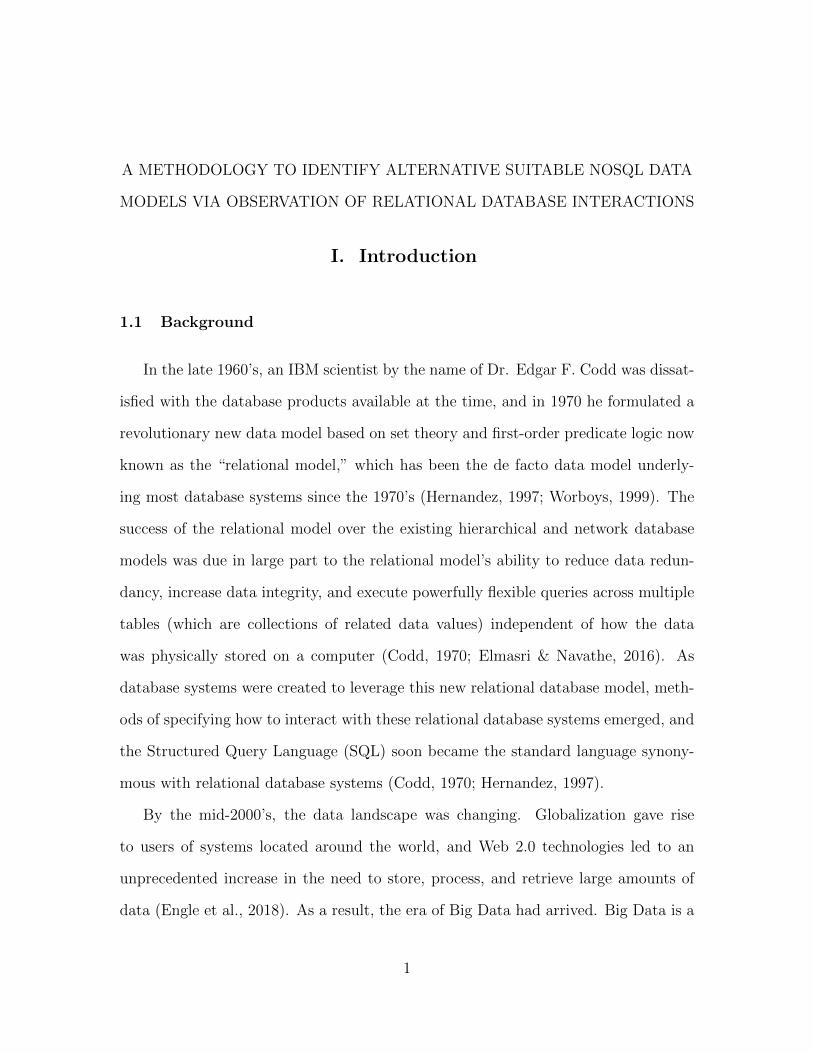
1.1 Background

In the late 1960’s, an IBM scientist by the name of Dr. Edgar F. Codd was dissat-

isfied with the database products available at the time, and in 1970 he formulated a

revolutionary new data model based on set theory and first-order predicate logic now

known as the “relational model,” which has been the de facto data model underly-

ing most database systems since the 1970’s (Hernandez, 1997; Worboys, 1999). The

success of the relational model over the existing hierarchical and network database

models was due in large part to the relational model’s ability to reduce data redun-

dancy, increase data integrity, and execute powerfully flexible queries across multiple

tables (which are collections of related data values) independent of how the data

was physically stored on a computer (Codd, 1970; Elmasri & Navathe, 2016). As

database systems were created to leverage this new relational database model, meth-

ods of specifying how to interact with these relational database systems emerged, and

the Structured Query Language (SQL) soon became the standard language synony-

mous with relational database systems (Codd, 1970; Hernandez, 1997).

By the mid-2000’s, the data landscape was changing. Globalization gave rise

to users of systems located around the world, and Web 2.0 technologies led to an

unprecedented increase in the need to store, process, and retrieve large amounts of

data (Engle et al., 2018). As a result, the era of Big Data had arrived. Big Data is a

1

term that encompasses the unique challenges associated with the marked increase in

the Volume, Variety, and Velocity of data being generated and stored by individuals,

governments, and corporations. Often referred to as the “3 V’s” of Big Data, these

attributes of Big Data present new challenges for processing (including the storage

and access of) this data (Dugane & Raut, 2014).

Volume refers to the quantity of data being processed (NIST Big Data Public

Working Group Definitions and Taxonomies Subgroup, 2015). Presently, there is no

agreed upon threshold (in terms of quantity of data) that must be achieved before this

criteria is met, however, various authors have cited values between a terabyte and a

petabyte (Schroeck et al., 2012) or at least 30-50 terabytes (Sawant & Shah, 2013) as

suggestions for quantifying the scale of Big Data. Regardless of the definition used, it

became evident that many existing traditional systems were struggling to cope with

handling these ever-increasing amounts of data via the traditional approach of vertical

scaling, and instead a new paradigm based on increasing storage and computational

power via horizontal scaling across distributed systems was required (NIST Big Data

Public Working Group Definitions and Taxonomies Subgroup, 2015).

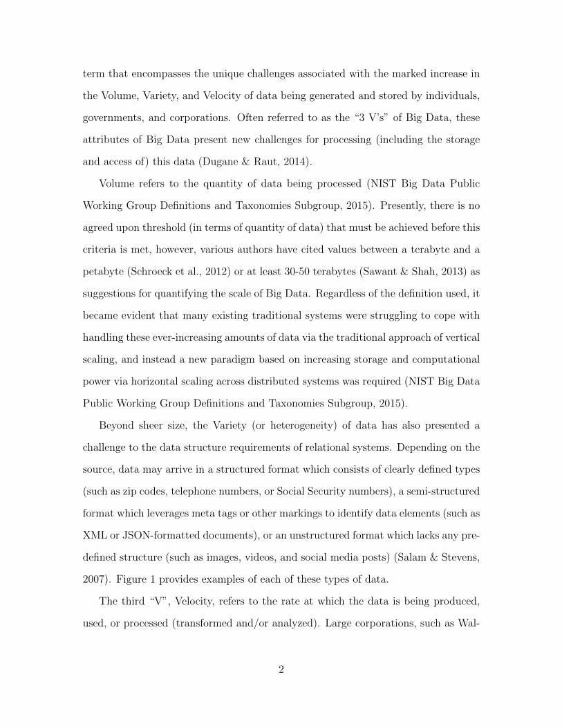
Beyond sheer size, the Variety (or heterogeneity) of data has also presented a

challenge to the data structure requirements of relational systems. Depending on the

source, data may arrive in a structured format which consists of clearly defined types

(such as zip codes, telephone numbers, or Social Security numbers), a semi-structured

format which leverages meta tags or other markings to identify data elements (such as

XML or JSON-formatted documents), or an unstructured format which lacks any pre-

defined structure (such as images, videos, and social media posts) (Salam & Stevens,

2007). Figure 1 provides examples of each of these types of data.

The third “V”, Velocity, refers to the rate at which the data is being produced,

used, or processed (transformed and/or analyzed). Large corporations, such as Wal-

2

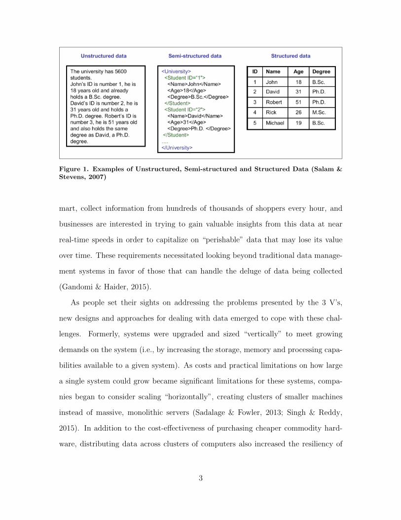
Figure 1. Examples of Unstructured, Semi-structured and Structured Data (Salam &Stevens, 2007)

mart, collect information from hundreds of thousands of shoppers every hour, and

businesses are interested in trying to gain valuable insights from this data at near

real-time speeds in order to capitalize on “perishable” data that may lose its value

over time. These requirements necessitated looking beyond traditional data manage-

ment systems in favor of those that can handle the deluge of data being collected

(Gandomi & Haider, 2015).

As people set their sights on addressing the problems presented by the 3 V’s,

new designs and approaches for dealing with data emerged to cope with these chal-

lenges. Formerly, systems were upgraded and sized “vertically” to meet growing

demands on the system (i.e., by increasing the storage, memory and processing capa-

bilities available to a given system). As costs and practical limitations on how large

a single system could grow became significant limitations for these systems, compa-

nies began to consider scaling “horizontally”, creating clusters of smaller machines

instead of massive, monolithic servers (Sadalage & Fowler, 2013; Singh & Reddy,

2015). In addition to the cost-effectiveness of purchasing cheaper commodity hard-

ware, distributing data across clusters of computers also increased the resiliency of

3

these systems since a failure in any given node could be compensated for by others

in the cluster (Sadalage & Fowler, 2013). It’s worth mentioning, however, that these

advantages in terms of distributed processing in order to achieve highly-scalable per-

formance were not achievable without certain trade-offs, such as relaxed consistency

constraints (Sullivan, 2015).

Beyond architectural considerations like horizontal scalability, a move towards

data models that were not based on the existing relational model also became a

necessary and relevant development (as well as the many database implementations

built upon them). Referred to by the moniker “NoSQL” (to set them apart from

the existing SQL-based relational model), these newer non-relational based systems

adopted fundamentally different data models from the traditional relational data

model (Evans, 2009; Sullivan, 2015). These new approaches enabled the develop-

ment of systems which helped solve problems that relational-based systems were now

struggling to answer (such as the cost and size limitations, mentioned earlier).

1.2 Motivation

Although the NoSQL data models (and the databases built upon them) were ini-

tially created in order to deal with large datasets residing on distributed systems,

previous research has highlighted the potential value of employing NoSQL databases

in non-distributed configurations (i.e., the database and any associated database man-

agement system software is hosted on a single box, but the system may still service

multiple users)(Beach et al., 2019; Engle et al., 2018). Some of the reasons proposed

for the use of such systems include “efficient write performance and fast, low-latency

access, among others” (Engle et al., 2018).

There are several possible scenarios where an existing system may be employing a

relational data model when a different data model would actually be more appropri-

4

ate. One possibility for this is that the application developer was unfamiliar with the

recent development of the NoSQL data models when they designed the system. Al-

ternatively, the usage of a database system may have evolved over time from a point

when a relational data model made the most sense, to something different which

now more closely aligns with a NoSQL data model. Whatever the reason, identifying

opportunities where a NoSQL data model may be more suitable for the purposes at

hand is one means of improving overall system performance. This research intends to

further explore the concept of using a NoSQL data model on non-distributed systems

by demonstrating how the usage of an existing relational database system can be

evaluated in order to determine if there may be a more suitable NoSQL data model

for that observed usage.

1.3 Problem Statement

While some technically-inclined users may be interested in the inner workings of a

database system, many users are less concerned with what is taking place “under the

hood” and instead care primarily about the usability and performance aspects of such

systems (Xie, 2003). Furthermore, system developers may not be well-versed in the

fairly recent emergence of NoSQL data models, and therefore they may not recognize

the potential benefits of employing these data models in their systems (Venkatraman

et al., 2016). For these reasons, the underlying data model of a database may not

align with the most suitable data model for a given use case.

Thus, a useful (yet presently lacking) capability for determining the suitability of

a database system involves identifying ways to better align the underlying storage,

processing and retrieval mechanisms towards the manner in which they are being

used, in a way that is as transparent as possible to the user or developer. This

research proposes a methodology to address this problem.

5

1.4 Research Questions & Hypotheses

The development of the methodology proposed in this research required a num-

ber of steps. First, it needed a means of characterizing how users are employing a

relational database management system in order to identify different aspects of us-

age which make various NoSQL solutions either more or less suitable for the current

usage. Secondly, it required an understanding of how to assess the suitability of a non-

relational database system based on that observed usage. Therefore, the overarching

goal of this research was to develop a methodology for characterizing the suitability

of the different NoSQL data models for a particular use case based on observations of

user interactions with an existing non-distributed (i.e., single-box) relational database

system. In order to further develop this methodology, the following questions were

proposed to guide this research.

1. Which observable criteria exist for assessing the usage patterns of a non-distributed

relational database in an automated fashion?

2. Using an automated methodology, can non-distributed relational database usage

patterns be mapped to more suitable data models using the observable criteria?

In order to support answering the stated research questions, this research also

sought to answer the following three hypotheses:

1. One or more elements of the Engle criteria (introduced in the next section) can

be mapped to observable characteristics of relational database systems.

2. It is possible to profile usage of a database based on observable characteristics

of a relational database system.

3. A set of decision criteria based on the observational profile can be incorporated

6

into a decision model that can characterize the suitability of a non-relational

(NoSQL) data model for the observed usage characteristics.

How these research questions and hypotheses will be addressed is now discussed

in the following section.

1.5 Methodology

Existing research conducted by Engle produced a normalized set of performance

priorities for the NoSQL and relational data models across 12 distinct criteria (here-

after termed “the Engle criteria”) (Engle, 2018). These criteria describe key char-

acteristics of a database’s usage for a particular use case such as Query Complexity

(QC), Query Omniscience (QO), Transparency (T), and so on (see Table 1 for the

full list; these criteria will be further discussed in Chapter 2). In that research, the

performance priorities for the 12 criteria were coupled with inputs from subject mat-

ter experts (SMEs) that were knowledgeable about the application being serviced by

a database (although the SMEs themselves were not experts in database systems)

through a multiple-criteria decision-making (MCDM) process called the Analytic Hi-

erarchy Process (AHP). The output of this process produced a list of “global priori-

ties” for each of the five data models, which represented the rank-ordered suitability

of each data model for the SMEs systems based on their inputs.

In this research, the performance priorities for the Engle criteria were again em-

ployed. However, in lieu of soliciting the relative importance rankings for each of

the Engle criteria from SMEs, observations of simulated system usage were used as

proxies to infer the degree to which each of the criteria is present. Specifically, SQL

queries and responses (i.e., any data returned from the DBMS in response to the

query) between a particular application and an existing relational database man-

agement system (RDBMS) were monitored and then parsed, and features of these

7

Table 1. Engle Criteria (Engle, 2018)

Criterion Description

Cross-Aggregate1 ConsistencyAbility of a DBMS to “perform cascading updatesacross data and relationships.”

Data Typing EnforcementAbility of a DBMS to apply schema enforcementof data types during transactions2.

Large Aggregate TransactionsAbility of a DBMS to “store, retrieve and updatelarge aggregates quickly” (>1 TB).

Small Aggregate TransactionsAbility of a DBMS to “store, retrieve and updatesmall aggregates quickly” (<1 kB).

ManipulationAbility of a DBMS to “update elements of storedaggregates independently from other aggregatesand elements.”

PlasticityAbility of a DBMS to “add or remove elementswithin stored aggregates.”

Pre-processingLevel of effort required to pre-process data intoDBMS (operations required to import/load data).

Structural MalleabilityAbility of DBMS to add/remove “types” ofaggregates.

TransparencyAbility of DBMS to “store aggregates such thatindividual elements within the aggregate can beviewed and retrieved during read transactions.”

Query3 ComplexityAbility of DBMS to “perform simple andcomplex queries.”4

Query Omniscience“Degree to which the complete set of possiblequeries is known by the user before system isimplemented.”

Result TimelinessSpeed in which results are returned to the userfollowing a request.

1 “An aggregate is formally defined as a composite data object that is considered the atomic unit forCreate, Read, Update and Delete (CRUD) operations” (Engle, 2018), borrowing from (Sadalage& Fowler, 2013).

2 A transaction is defined as “a [single] CRUD operation performed on a single aggregate” (Engle,2018).

3 A query is defined as “an action performed on a database, using a language such as SQL, toaccess a specific set of data” (Engle, 2018), borrowing from (Baker, 2011; Codd, 1970).

4 “A simple query retrieves data using only a unique identifier and/or values. Complex queriesinvolve additional conditions enforced on the operations” (Engle, 2018).

observed interactions were extracted using a tool built during the course of this re-

search called the “Engle Criteria Analysis Tool” (ECAT) in order to produce counts

of observed attributes for each of the criteria and ultimately, their relative weighted

8

metrics. Finally, by employing a MCDM process known as Simple Additive Weighting

(SAW) (Yoon & Hwang, 1995), the performance priorities and the extracted weighted

metrics were joined to generate a decision model reporting the suitability rankings

for each of the data models.

Figure 2 provides a high-level overview of the timeline of events for this methodol-

ogy. In the first step, the system’s database usage is captured. System users interact

with an application (such as a web or desktop application) which interfaces with a

back-end database in order to provide access to the necessary data. While the ap-

plication is interfacing with the database, the data packets traversing the network

between the application and the database are observed and captured. In step 2, this

packet capture is then used as an input to the ECAT which parses the packet capture

to extract the relative counts for each of the Engle criteria and produces a normalized

vector of Engle criteria metrics. In the third and final step, these metrics are used as

an input into a SAW decision model in order to produce a rank-ordered output listing

for each of the five data models (relational, document, key-value, columnar-oriented,

and graph) characterizing the suitability of each for the observed usage.

Figure 2. Methodology Timeline

9

Assumptions/Limitations.

Presently, the software that was developed for this methodology relies on third-

party software (called Percona Toolkit) in order to parse and extract SQL queries from

RDBMS packet captures. This software is currently only capable of parsing MySQL

network packets, so a current limitation to this approach is that the observed usage

must be observed between a MySQL RDBMS and its user(s)/application(s) (Percona,

LLC., 2020b). It should be noted this is a limitation based on the current software

implementation, not the methodology.

Furthermore, there is currently no way to differentiate between different users or

applications interacting with a given database, so for the purposes of this research

all observed usage is assumed to be restricted to a single application and database

on an RDBMS. While there is no way to isolate traffic between different applications

within ECAT, this assumption could potentially be enforced in real-world systems by

segmenting the specific network traffic between the RDBMS and the application and

ensuring only a single database on the RDBMS is being queried in order to isolate

only the traffic of interest.

Implications.

The methodology suggested in this dissertation proposes a novel approach for pas-

sively observing RDBMS usage and attempting to characterize that usage through

those observations alone. Although some of the tools and techniques used in this re-

search have been used by database administrators to analyze characteristics of specific

MySQL queries, a lack of similar approaches in the literature suggests that this tech-

nique represents a previously unseen method towards characterizing the generalized

usage of a database.

Furthermore, since this approach requires no direct input from system users, it has

10

the advantage of being able to produce objective insights about how a given system

is being utilized by all users, either at a particular snapshot in time or to observe how

that usage is evolving over time. Finally, this methodology has the potential to be

opportunistically applied by system owners who are looking for possible solutions to

improve system performance or enhance system usability by adopting a more suitable

underlying data model.

Preview.

This dissertation is organized such that each chapter builds upon the previous one.

Chapter 2 lays the foundation by providing a review of key concepts and previous re-

search that this work has been built upon. In Chapter 3, the proposed methodology is

introduced to include a discussion of how ECAT’s instrumentation monitors, collects,

and processes the observed usage data, how the three use case simulations that were

developed for this research were used to generate the representative real-world data

and demonstrate ECATs application. Then, a discussion of the relationships between

the Engle criteria and the data models is offered, and finally Chapter 3 concludes

with a pilot study validating that the ECAT software adequately characterizes the

usage of a system based on controlled inputs. Chapter 4 then presents the findings

of the three use case simulations that were previewed in the third chapter. Finally,

Chapter 5 concludes this research with a summary of findings, their significance, and

recommendations for future research.

11

II. Literature Review

2.1 Chapter Overview

The purpose of this chapter is to provide a brief introduction to some of the key

concepts relating to the proposed research. First, an introduction to the relational

and NoSQL data models is explored. Secondly, use cases for each of the NoSQL

models are provided. The third section offers an exploration of current approaches for

characterizing database usage patterns. Then, a discussion of postulated mappings

between the Engle criteria and observable attributes is presented, followed by an

overview of the Simple Additive Weighting decision model. Finally, the proposed

research hypotheses are offered.

2.2 Database Systems

What is a database? Fundamentally, in order to be useful a database must be

able to do two things: “when you give it some data, it should store the data, and

when you ask it again later, it should give the data back to you” (Kleppmann, 2017).

Figure 3 shows how various database components (the database(s), DBMS and

database applications) join together to create a database system. Databases are col-

lections of related data. However, this alone is not useful without a way of interacting

with this data or understanding how the data is stored together. Therefore, a database

management system (DBMS) is also typically required, along with a description of

the “data types, structures, and constraints of the data to be stored in the database”

in the Stored Database Definition (also called the meta-data) (Elmasri & Navathe,

2016).

A DBMS is a “general-purpose software system that facilitates the process of

defining, constructing, manipulating, and sharing databases among various users and

12

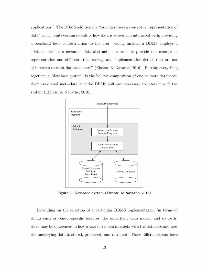
applications.” The DBMS additionally “provides users a conceptual representation of

data” which omits certain details of how data is stored and interacted with, providing

a beneficial level of abstraction to the user. Going further, a DBMS employs a

“data model” as a means of data abstraction in order to provide this conceptual

representation and obfuscate the “storage and implementation details that are not

of interests to most database users” (Elmasri & Navathe, 2016). Putting everything

together, a “database system” is the holistic composition of one or more databases,

their associated meta-data and the DBMS software necessary to interact with the

system (Elmasri & Navathe, 2016).

Figure 3. Database System (Elmasri & Navathe, 2016)

Depending on the selection of a particular DBMS implementation (in terms of

things such as vendor-specific features, the underlying data model, and so forth)

there may be differences in how a user or system interacts with the database and how

the underlying data is stored, processed, and retrieved. These differences can have

13

significant impacts on the strengths and weaknesses of a database system, and can

dictate whether or not a particular database system is suitable for a given task.

Additionally, application programs may be considered part of a database system

as they interact with databases by querying the DBMS. “Query” has often been

understood to refer to a request for data from a system. Commands sent to a database

system to create or modify data have been called transactions (Elmasri & Navathe,

2016). According to the standards document that codifies the SQL language, “SQL-

statement” is used to refer to the strings of characters that conform “to the Format

and Syntax Rules specified in one of the parts of ISO/IEC 9075” (Melton, 2003).

For simplicity, in this document “query”, “statement”, or “command” shall be used

interchangeably to mean any instructions sent to the database, whether the purpose

is to create data, modify data, or retrieve data.

Relational Data Model.

As mentioned in the Introduction, databases built upon the relational data model

have been the dominant form of data storage for many years, due in large part to their

ability to reduce data redundancy (i.e., storing the same data in multiple locations),

increase data integrity (e.g., by enforcing constraints on what type of data can be

stored, ensuring that each row contains a unique value for a particular field, or by

requiring that a certain data field must be related to another one), execute powerfully

flexible instructions on a database, and consolidate data from multiple tables at query

time (Elmasri & Navathe, 2016). In fact, there is a common misconception that the

relational data model derives its name from the fact that these tables can be joined

at query time (i.e., “related”); in actuality, “relation” is a term borrowed from the

mathematical set theory upon which the model was based. In typical usage, “relation”

is commonly observed to be synonymous with “table” (Hernandez, 1997; Pratt, 2005).

14

One of the key features of the relational model is that data organized as tabular

rows and columns is aggregated from smaller tables consisting of rows of tuples.

Tuples represent records, or individual rows of data, and are a rigid data structure that

do not allow for the nesting of other tuples within them (Hernandez, 1997; Sadalage

& Fowler, 2013). This is in contrast to the aggregate-oriented model common in many

NoSQL data models, discussed below.

The process of decomposing data into smaller subsets is called “normalization,”

and it is intended to avoid storing redundant data, which also helps ensure the in-

tegrity of the data as it is inserted, updated, or deleted. These were key design

features when Dr. Codd developed the model. The process of normalization occurs

during the design phase the database and typically requires that tables contain one or

more fields that uniquely identify each of the records that it contains (called a “pri-

mary key”). Tables may also have fields defined as a “foreign key” that are used to

reference the primary keys in another table, enabling a relationship to be established

between the two tables (Hernandez, 1997).

Another key design feature for relational databases are to guarantee ACID trans-

actions. A transaction refers to “logical units of database processing” that specify

“one or more database accesses, such as reading or updating of database records”

which “must be executed in its entirety to ensure correctness” (Elmasri & Navathe,

2016). ACID refers to four desirable properties found in relational databases: Atom-

icity (transactions occur as an indivisible, atomic unit), Consistency (transactions

are not able to violate integrity constraints in the system), Isolation (transactions in

a system are not visible to concurrent users until the transaction is complete), and

Durability (once a transaction has completed, the data will remain present even in

the event of a disruption such as a power loss) (Sullivan, 2015). These properties are

desirable because they help ensure the predictability and integrity of the data, but

15

these are not the only way relational databases seek to address data integrity.

Primary and foreign keys are two kinds of integrity constraints that a relational

database can enforce. For example, a RDBMS may not allow a user to insert a new

record into a table if that record has a foreign key value that does not exist as a

primary key in the referenced table. Additionally, a third type of constraint that can

be specified in relational databases are “legal values.” These restrict the values that

may be entered in the database in order to ensure the values comply with business

rules. An example of this type of constraint would be the requirement that a salary

field contain only positive numerical values, or that a customer’s shipping state match

a state that a company actually ships products to (Hernandez, 1997; Pratt, 2005).

Users typically use the Structured Query Language (SQL) to express queries

within relational databases, and as such, SQL has become practically synonymous

with relational databases over time (Redmond & Wilson, 2012). Table 2 provides

a list of common SQL commands and functions that are also referenced throughout

this document. For instance, the SELECT command is one of the most fundamental

SQL commands because it is used to retrieve data from the DBMS. As an illustrative

example, envision a hypothetical database containing student records called “cur-

rent students”. A query to retrieve a list of all student names and their respective de-

partments who are expecting to graduate this year might look like: “SELECT name,

department FROM current students WHERE anticipated graduation year = 2020”.

A query to update a student’s major might look like: “UPDATE current students

SET major = ‘Systems Engineering’ WHERE student id = 12345”. Examples of

some popular relational database management systems that employ various forms of

SQL include Oracle, MySQL, Microsoft SQL, and PostgreSQL (solid IT, 2019).

16

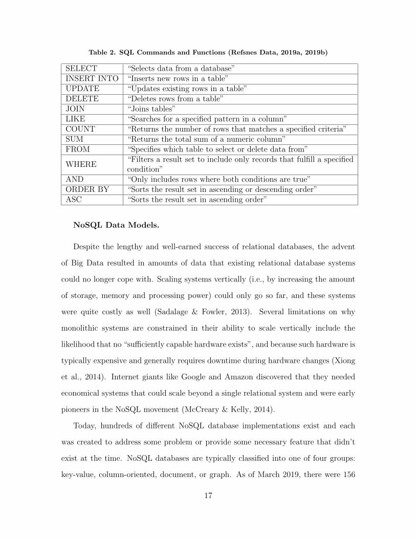
Table 2. SQL Commands and Functions (Refsnes Data, 2019a, 2019b)

SELECT “Selects data from a database”INSERT INTO “Inserts new rows in a table”UPDATE “Updates existing rows in a table”DELETE “Deletes rows from a table”JOIN “Joins tables”LIKE “Searches for a specified pattern in a column”COUNT “Returns the number of rows that matches a specified criteria”SUM “Returns the total sum of a numeric column”FROM “Specifies which table to select or delete data from”

WHERE“Filters a result set to include only records that fulfill a specifiedcondition”

AND “Only includes rows where both conditions are true”ORDER BY “Sorts the result set in ascending or descending order”ASC “Sorts the result set in ascending order”

NoSQL Data Models.

Despite the lengthy and well-earned success of relational databases, the advent

of Big Data resulted in amounts of data that existing relational database systems

could no longer cope with. Scaling systems vertically (i.e., by increasing the amount

of storage, memory and processing power) could only go so far, and these systems

were quite costly as well (Sadalage & Fowler, 2013). Several limitations on why

monolithic systems are constrained in their ability to scale vertically include the

likelihood that no “sufficiently capable hardware exists”, and because such hardware is

typically expensive and generally requires downtime during hardware changes (Xiong

et al., 2014). Internet giants like Google and Amazon discovered that they needed

economical systems that could scale beyond a single relational system and were early

pioneers in the NoSQL movement (McCreary & Kelly, 2014).

Today, hundreds of different NoSQL database implementations exist and each

was created to address some problem or provide some necessary feature that didn’t

exist at the time. NoSQL databases are typically classified into one of four groups:

key-value, column-oriented, document, or graph. As of March 2019, there were 156

17

different implementations of these four database types being tracked on the popular

database ranking website db-engines.com and 225 on the more specialized website

nosql-database.org (solid IT, 2019).

As mentioned above, many of the NoSQL data models follow a different approach

to organizing data than the relational model in that they are aggregate-oriented. The

term “aggregate” has been borrowed from Evans’ Domain-Driven Design, whereby

“an aggregate is a collection of related objects that we wish to treat as a unit”

(Sadalage & Fowler, 2013). In particular, the key-value, document, and column-

oriented data models are considered to be aggregate-oriented. By dealing with data

in the form of aggregates, data that is related can be stored together to help improve

retrieval performance through locality and denormalization (i.e., the same data may

be stored in multiple locations in order to minimize the number of aggregates needing

to be accessed, thus speeding up read times) (Sadalage & Fowler, 2013).

One important consequence of aggregate boundaries is that they define the bounds

for what can be updated in a single transaction. Unlike the ACID guarantees of rela-

tional databases which allowed for the manipulation of many rows spanning multiple

tables to occur in a single transaction, the three aggregate-oriented databases (i.e.,

key-value, document, and column-oriented) do not guarantee that updates spanning

multiple aggregates will execute as an atomic operation (Sadalage & Fowler, 2013).

Key-Value Data Model.

Key-value is the simplest NoSQL data model, whereby stored values are retrieved

by providing the unique key that has been associated with that value. Keys can

take on a wide variety of forms such as a string of characters, however, the one

required property for them is that each is unique from every other key within a given

namespace (which is a collection of key-value pairs), so that they can uniquely identify

18

the associated value being stored (Sullivan, 2015). In the key-value data model, the

key serves as an identifier to access the aggregate (i.e. value) of interest (Sadalage &

Fowler, 2013).

Meanwhile, the value stored in a key-value database can be virtually any set of

bytes, including “integers, floating-point numbers, strings of characters, binary large

objects (BLOBs), semi-structured constructs such as JSON objects, images, audio

and just about any other data type you can represent as a series of bytes” (Sullivan,

2015). Common uses of the key-value data model include document and file stores,

dictionaries, and lookup tables (McCreary & Kelly, 2014). The image in Figure

4 shows a key-value data model with four entities (in reality, what is depicted is

actually more of a meta-model representing one possible way to structure data, as

the “userID” field would actually be some unique value that relates to a particular

person). An entity is a representation of “a real-world object or concept ... that is

described in the database” (Elmasri & Navathe, 2016).

Figure 4. Key-Value Data Model

Owing to the simple design of the key-value data model, implementations of this

model tend to operate quickly and are easy to employ. One of the drawbacks to

this simplistic design is that key-value stores do not support queries on values, but

19

rather only on the keys. Also, since the data model does not know or consider what

kind of data is being stored, it is up to the application developer to determine the

type of data being stored (e.g., text string, binary image, XML file, etc.) (McCreary

& Kelly, 2014). Some of the implications of this are that it is now the application

developer’s responsibility to keep track of the keys used to reference the data, as well

as determining how to process and manipulate the data once it is retrieved from the

database(Sadalage & Fowler, 2013). Redis, DynamoDB and Memcached are presently

three of the most popular Key-Value databases (solid IT, 2019).

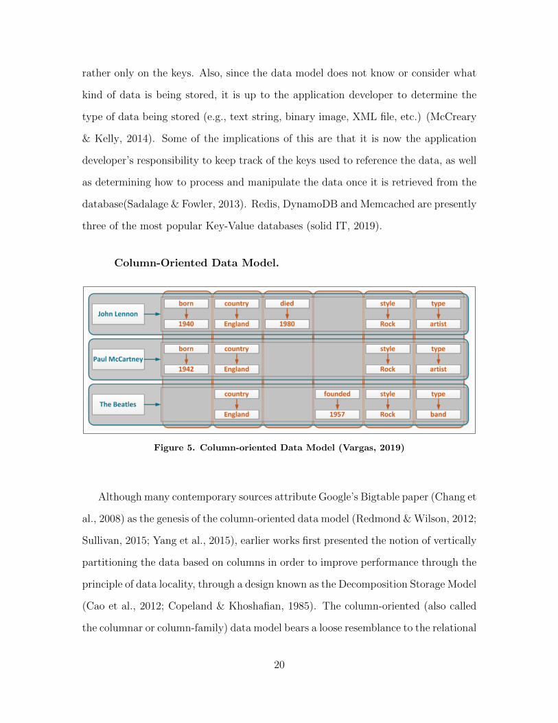
Column-Oriented Data Model.

Figure 5. Column-oriented Data Model (Vargas, 2019)

Although many contemporary sources attribute Google’s Bigtable paper (Chang et

al., 2008) as the genesis of the column-oriented data model (Redmond & Wilson, 2012;

Sullivan, 2015; Yang et al., 2015), earlier works first presented the notion of vertically

partitioning the data based on columns in order to improve performance through the

principle of data locality, through a design known as the Decomposition Storage Model

(Cao et al., 2012; Copeland & Khoshafian, 1985). The column-oriented (also called

the columnar or column-family) data model bears a loose resemblance to the relational

20

data model in that it consists of tables with rows and columns, however, there are some

key architectural differences. Rows and columns are employed as lookup keys in this

data model (which can also be considered as a two-level map), enabling the system to

sparsely populate only the values that are present (a key improvement over relational

database implementations which are not efficient at sparsely storing data where fields

in a tuple do not contain any data) (McCreary & Kelly, 2014). The column-oriented

data model also organizes data into column families, which helps keep columns of

data that are likely going to be accessed together close to each other, improving query

performance due to the locality of the data (Sullivan, 2015), although the increasing

adoption of solid-state storage technology is mitigating the impact of this aspect.

Like the key-value data model, the column-oriented data model allows for the efficient

storage and retrieval of data across distributed systems, which is a trait common to

most NoSQL data models (graph databases being a notable exception) (McCreary &

Kelly, 2014). The image in Figure 5 shows a column-oriented data model containing

three rows and six columns. Note that not all columns contain all rows, demonstrating

this data model’s ability to sparsely store only the data of interest. Cassandra and

HBase are two of the most popular column-oriented datastores (solid IT, 2019).

Document Data Model.

The document data model employs a similar design as the key-value data model

(i.e., specifying a unique key will return its associated value), but the document

itself is considered a collection of key-value pairs. A key difference between this data

model and the key-value data model is that the document data model also allows for

the storage and retrieval of hierarchically organized data (e.g., XML, JSON) making

it extremely flexible, generalizable, and popular (McCreary & Kelly, 2014; Sullivan,

2015). Implementations of the document data model organize documents into related

21

sets called collections, which are somewhat analogous to the concept of a table in the

relational data model, while the documents themselves are analogous to the rows.

Another difference from the key-value model is that stored values in the docu-

ment model are not considered opaque; they can be queried on which enables full-

text search capabilities (Khazaei et al., 2016). Since the aggregate boundary for the

document model is the document itself, it is unable to provide the capability of up-

dating multiple documents in a single atomic action (Khazaei et al., 2016; Sadalage

& Fowler, 2013). However, the transparent nature of the aggregate-oriented docu-

ment data model means that it is possible to perform queries against data elements

stored within a document (as opposed to having to address or manipulate the entire

document itself), which can simplify the process for the user and reduce the overhead

that might otherwise be required for processing unnecessary data (Sullivan, 2015).

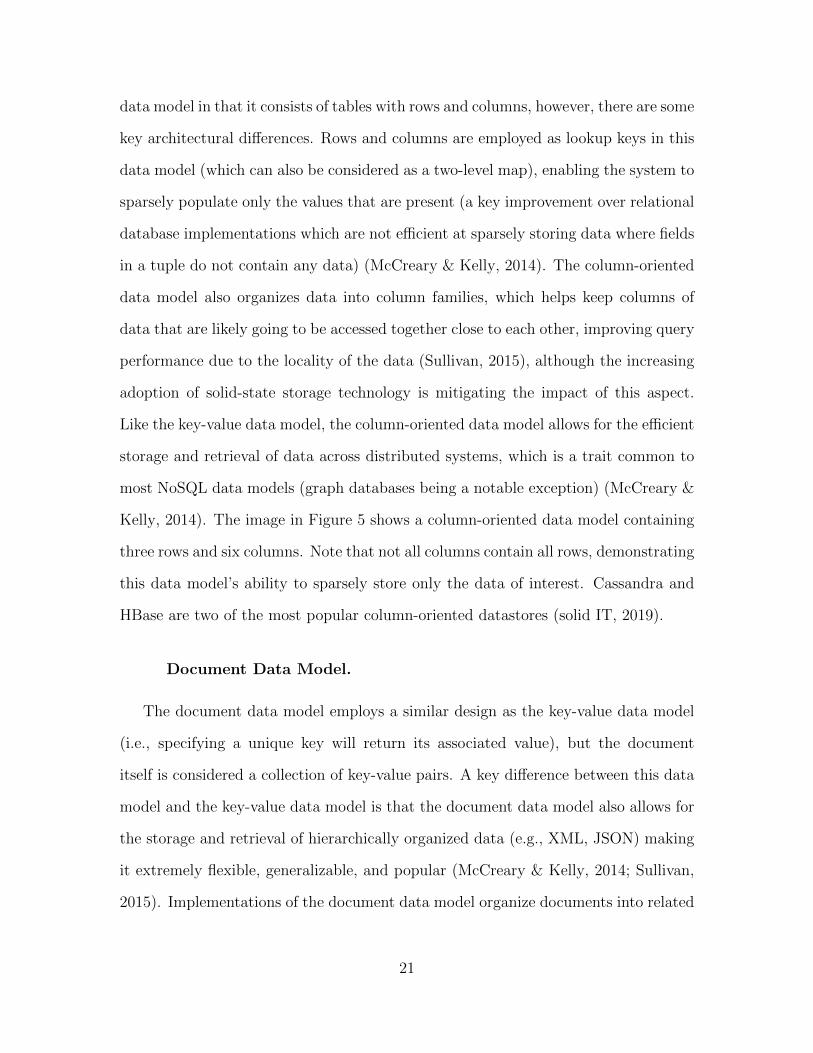
Figure 6. Document Data Model (Vargas, 2019)

The image in Figure 6 represents an example document with a number of fields;

some containing a single value (e.g., ‘Paul’, 447557505611, ‘London’) and others con-

22

taining more complex structures such as an array of strings, or even another nested

document (e.g., ‘Cars’) with sub-documents of its own. Presently, the most popular

document database is MongoDB (solid IT, 2019).

Graph Data Model.

The graph data model stores data in two kinds of elements: as vertices, and as

connections between vertices (also called edges or arcs). The highly-interconnected

nature of elements in the graph data model makes it useful for storing relationship-

heavy data, where different data elements have a high degree of interconnections

such as commonly found in social networks and rules-based engines. However, it also

means that unlike the other NoSQL models previously discussed, implementations of

the graph data model are not well suited for distributed processing applications due

to the heavily connected nature of individual nodes in a graph. In fact, one of the

often-touted strengths of NoSQL data models is their ability to scale horizontally in

distributed systems. However, the aggregate-ignorant nature of the graph data model

makes it difficult to effectively draw boundaries around elements of data (since this

model is all about creating relationships, not boundaries). For example, if a graph

database grows to the point where it cannot be hosted on a single machine, then

as the database tries to follow edges between vertices it is likely that these traversal

operations will span across machines, which will adversely impact performance. As

a result, it is more difficult to horizontally scale graph databases than the key-value,

document, or column-oriented data models (Sadalage & Fowler, 2013; Sullivan, 2015).

Edges and vertices are both capable of storing data in this model (for instance,

you can add weights or directions1 to edges). This provides the data model with

the ability to model many real-world problems such as social networks (e.g., where

1Edges can be directed, which represents a one-way relationship between two nodes, or undirectedwhich assumes that the relationship makes sense in both directions (Sullivan, 2015).

23

vertices represent people and directed edges define their relationships, as in “Jim”

is the supervisor of “John”) or transportation systems (e.g., vertices represent cities

and weighted edges represent the distances between them, as in “Dayton, OH” is 16

miles from “Xenia, OH”) (Sadalage & Fowler, 2013; Sullivan, 2015).

The image in Figure 7 shows an example of the graph data model with seven

vertices interconnected by six directed edges (Vargas, 2019). Neo4J solidly remains

the most popular graph database for the time being (solid IT, 2019).

Figure 7. Graph Data Model (Vargas, 2019)

NoSQL on a Single Machine.

Although many of the commonly cited reasons for using NoSQL models are cen-

tered around their use in distributed environments (e.g., for scalability across com-

modity hardware), there are several compelling reasons to consider their use on non-

distributed (i.e., single-box) deployments as well. For example, the rigid structure of

relational databases often require that arriving data must be properly formatted (i.e.,

having a similar structure in terms of delineated values conforming to expected data

types) in order to comply to the existing schema. This process, known as extract,

transform, and load (ETL) can impose upfront costs in terms of time, effort, and

computational overhead in order to do so. By contrast, NoSQL data models are able

24

to accept heterogeneous2 forms of data, decreasing the amount of data pre-processing

over that which would be required in a relational data model (Sawant & Shah, 2013).

Additionally, this also allows for the storage of the data in a form closer to which it

originally arrived in which may facilitate later retrieval. Finally, it affords a great deal

of flexibility to change over the relational model, as elements within an aggregate can

be added or removed without concern to modifying the rest of the existing database

(Engle et al., 2018).

Beyond simply being adaptable to changes, the schemaless nature of NoSQL data

models means they are also well suited for supporting multiple types of data struc-

tures. As described above, key-value stores are agnostic regarding what kind of data

is being stored, which can vary from a single binary value to a more complex data

structure like a list from one aggregate to the next. Document databases extend this

flexibility with their ability to represent complex hierarchical structures, commonly

represented in formats such as XML or JSON. The raison d’etre for column-oriented

databases is that they provide efficient storage and retrieval of related data by group-

ing data into, unsurprisingly, column families. Graph databases, being focused on

the interconnected nature of related data, similarly can store vastly different kinds of

data from one node or edge to another (Engle et al., 2018; Sadalage & Fowler, 2013).

The highly structured nature of the Structured Query Language affords users

with a well-defined means of interacting with relational databases and some of the

key features it provides (namely things like the joining of tables and assuring the

integrity of data). While some implementations of NoSQL databases have attempted

to make the transition easier for developers by adopting SQL-like interfaces, the ability

for NoSQL to operate independently from SQL means that access to these databases

can be achieved in ways that are simpler for the developer, such as via application

2“Heterogenous” is another way of referring to data variety (Allen, 2015).

25

programming interfaces (APIs) or web-based (i.e., HTTP or REST-based) interfaces

(Engle et al., 2018; Redmond & Wilson, 2012; Sadalage & Fowler, 2013).

One key insight from all this is to ultimately recognize that “NoSQL is driven

by application-specific access patterns” (Engle et al., 2018). A component of this

research will focus on how to identify these access patterns as a means of determining

the suitability of a data model based on observed usage.

2.3 Typical NoSQL Use Cases

In this section, common use cases for NoSQL data models are introduced. This

discussion will highlight some of the benefits and shortcomings of each of the data

models in the context of the proposed criteria.

Key-Value - Session Management, User Profiles, and Shopping Carts.

The central premise of the key-value data model is that it is focused around

“simple read and write operations to a data item that is uniquely identified by a key”

(DeCandia et al., 2007). Thus, it follows that ideal circumstances in which one would

desire to employ this model will involve cases where some unique entity (i.e., it can

be represented by a unique key) refers to a collection of data that will generally be

interacted with as an atomic unit (i.e., the collection of data it refers to is considered

aggregate-oriented).

Several use cases that are ideal in this context include session management, user

profiles, and shopping carts (DeCandia et al., 2007; Sadalage & Fowler, 2013; Sri-

vastava & Shekokar, 2016). For instance, all three typically employ some kind of

unique identifier per user (e.g., a session id or user id), so they are ideally suited to

perform key-based lookups in order to retrieve value(s) of interest. This holds as long

as the application is only concerned with operating on a single user’s data at a time,

26

since the key-value model does not allow operating across multiple keys in a single

transaction, nor does it handle relationships across different sets of data (Sadalage &

Fowler, 2013). Finally, it is unlikely that any of these applications would generally3

require the ability to conduct complex queries based on stored values, which of course

is not possible with this data model.

Document - Event Logging, Content Management Systems, and E-

Commerce Applications.

The flexible schema and the ability to natively store semi-structured or unstruc-

tured data make the document data model well suited to a number of applications,

including event logging, content management systems, and e-commerce applications.

Event logs are likely to contain many semi-structured fields that will vary in con-

tent and structure depending on the application generating them, and as software

evolves over time the data these logs capture may also need to change. Similarly,

the dynamic nature of websites, blogging platforms, and web forums means they also

have a need to store semi-structured data in a way that is flexible to changes in the

future. Finally, the ability to store online orders in a denormalized state, as well as

allowing for evolution in product catalogs as new models are offered means that many

E-commerce applications can also benefit from this data model (Sadalage & Fowler,

2013).

Column-oriented - Event Logging and Content Management Systems.

Similar to the reasons listed above for the document data model, the column-

oriented data model’s flexibility in storing a variety of data structures and their

3It is certainly conceivable that an interesting query could be generated that would requiresearching by value (such as wanting to know how many users have a particular hot-selling item intheir shopping cart at any given time), however, this would not be considered the primary purposeof an online shopping cart and thus it does not negate the argument that a shopping cart is ideallysuited here.

27

ability to group related fields into column-families also makes them a good candidate

for event logging or content management system applications. The key determinant

for whether a column family would be suitable in these applications centers around

the application developer’s ability to define appropriate column-families based on ex-

pected usage patterns. Since real-world applications may involve hundreds of columns

or more, poor selection of column family clusters may result in accessing (and thus,

expending extra resources) unnecessary data if they are too broad, or having to look

up multiple column families to retrieve all of the necessary data (which may also

increase the required time) if they are defined too narrowly (Yang et al., 2015).

Graph - Social Networking and Recommendation Systems.

The graph data model is quite unlike the other NoSQL data models in several

key aspects. First of all, it is not aggregate-oriented like the other NoSQL data

models but rather is considered aggregate-ignorant (as is the case with the relational

data model). “Aggregate-ignorant” means that there is not a well-defined aggregate

structure providing clear boundaries around the data. This is not to say this is an

undesirable trait; rather it just means that it may be a good choice when there is

not going to be a commonly used structure for organizing and interacting with the

data. As a consequence, considering which data fields will be accessed together is

less important for this data model than with the previously mentioned data models.

Instead, this data model was designed to excel in describing relationships between

highly interconnected data (Sadalage & Fowler, 2013). While it is possible to capture

these same interrelationships in a relational data model, these often come at the

cost of performing joins which can become computationally expensive to perform,

particularly on large tables (Sullivan, 2015).

Therefore, it naturally follows that the ideal use cases for this data model are

28

applications like social networking sites and recommendation systems, which rely on

being able to quickly and easily make connections between various entities. Social

networks and recommendation systems (containing linkages between elements such

as individuals, their likes and preferences, etc.) typically evolve over time, but since

much of the work in creating these linkages between elements is done at insert time

(as opposed to query time) this means that the performance of this model for queries

would be much better than if this data was being queried in a relational system

(which would likely require expensive joins based on multiple foreign keys) (Sadalage

& Fowler, 2013).

2.4 Characterizing Database Usage Patterns

Users will interact with systems in a variety of ways depending on their needs

from the system and the variety of features the system offers. Systems with few

features and/or users may be used infrequently, while complex systems with many

users may be used more intensively. The actual usage patterns a database system is

experiencing will shift depending on how users are interacting with a system, owing to

factors such as changes in the types and frequency of users’ requests (Cooper, 2001).

In order to develop a methodology for determining suitable NoSQL data models

based on observed usage, an objective set of criteria for measuring this usage become

a necessary prerequisite. This research considers the application of an existing set

of criteria called the Engle criteria in order to characterize the usage of an existing

relational database.

Engle Criteria.

As introduced in Chapter 1, the “Engle criteria” refers to a set of 12 evaluation cri-

teria that were proposed in the 2018 PhD dissertation of Dr. Ryan Engle (listed again

29

in Table 3 for convenience). Collectively, these criteria are intended to characterize

functional “relational and NoSQL database traits” (as opposed to other system traits

such as security, affordability, etc.) that are relevant when considering applications

in a single computer environment (Engle, 2018).

Table 3. Engle Criteria (Engle, 2018)

Criterion Description

Cross-Aggregate ConsistencyAbility of a DBMS to “perform cascading updatesacross data and relationships.”

Data Typing EnforcementAbility of a DBMS to apply schema enforcementof data types during transactions.

Large Aggregate TransactionsAbility of a DBMS to “store, retrieve and updatelarge aggregates quickly” (>1 TB).

Small Aggregate TransactionsAbility of a DBMS to “store, retrieve and updatesmall aggregates quickly” (<1 kB).

ManipulationAbility of a DBMS to “update elements of storedaggregates independently from other aggregatesand elements.”

PlasticityAbility of a DBMS to “add or remove elementswithin stored aggregates.”

Pre-processingLevel of effort required to pre-process data intoDBMS (operations required to import/load data).

Structural MalleabilityAbility of DBMS to add/remove “types” ofaggregates.

TransparencyAbility of DBMS to “store aggregates such thatindividual elements within the aggregate can beviewed and retrieved during read transactions.”

Query ComplexityAbility of DBMS to “perform simple andcomplex queries.”

Query Omniscience“Degree to which the complete set of possiblequeries is known by the user before system isimplemented.”

Result TimelinessSpeed in which results are returned to the userfollowing a request.

Engle studied and assigned relative performance rankings to all 12 of these criteria

for each of the NoSQL data models as well as the relational data model. The relevance

of these criteria to this proposed research will be discussed in greater detail in Section

30

2.5, but an example of how to interpret these performance rankings is warranted here.

For example, Figure 8 contains a heat map based on a subset of the performance

priorities assigned by Engle for each of the criteria (the numerical scores that were

used to produce this map will be discussed and employed later in the SAW decision

model). In this figure, the column “RT” refers to the Result Timeliness criterion,

which is the speed in which results are returned to the user following a request (Engle,

2018). For this criterion, the Key-Value (KV) data model is coded green to indicate

that this data model is well supported by this criterion. Another way of interpreting

this is to say that if result timeliness is an important factor to you, then the key-value

data model would be more suitable than any of the alternatives. This interpretation

would seem to agree with other literature that suggests one of the primary strengths

of the key-value model is the speed at which they operate (Sullivan, 2015).

Figure 8. Heat Map, Observable Engle Performance Priorities vs. Data Models (Engle,2018)

In addition to generating relative performance priorities for each of the criteria,

Engle’s work leveraged the insights of several Subject Matter Experts (SMEs) who

were familiar with desirable characteristics of a database system for their given mis-

sions. These SMEs were interviewed and asked to provide pairwise comparisons of

31

each of the 12 criteria, evaluating their relative importance based on how each would

pertain to a desired log storage system for an Unmanned Aerial System (UAS). By

combining his research into the performance ratings along with the importance pri-

orities for each of the criteria reported by the SMEs, he was able to derive a rank-

ordered list of global priorities for each data model, based on the perceived needs of

each SME. This process was accomplished by using a MCDM process known as the

Analytic Hierarchy Process (AHP) (Engle, 2018; Saaty, 1980).

A significant motivation behind this research was the belief that it is possible to

infer which of these criteria are important to the system’s users based on observing

their relative presence or absence in the usage an existing system. Once observed, it is

then also possible to automate the process of determining which, if any, of the NoSQL

data models would be well suited for the existing application (and notably, without

the requirement to obtain inputs from system SMEs). Therefore, a key contribution of

this work focused on developing ways of assessing these criteria solely through obser-

vations of a user’s interactions with an RDBMS. Accordingly, this research has been

scoped to focus solely on assessing the usage of non-distributed relational database

systems.

2.5 Relation of Engle Criteria to Data Models

Based on the preliminary research highlighted above about the NoSQL data mod-

els and the relative strengths and weaknesses of each data model, initial efforts in

this research sought to identify the strongest mappings between each of the NoSQL

data models and the proposed database usage characterization criteria, as this was an

important precursor towards identifying which observable characteristics would later

support each of the data models. In addition to the discussion below, referencing back

to Figure 8 provides the reader with a summarized view of whether a given criteria

32

strongly supports (green), moderately supports (yellow/orange), or weakly supports

(red) the suitability of a given data model when there are indications that particular

criterion is present in the observed usage. Three of Engle’s criteria (Pre-processing,

Large Aggregate Transactions, and Small Aggregate Transactions) have been omitted

from this figure since they were not ultimately used in this methodology (as explained

in the individual criterion sections below).

Cross-Aggregate Consistency.

This criterion refers to the ability of a DBMS to “perform cascading updates

across data and relationships” (Engle, 2018). In reality, the definition of an aggregate

discussed earlier highlights the fact that aggregates are already considered atomic

units in terms of how they are operated upon. As such, for aggregate-oriented data

models (i.e., key-value, document, and column family) if changes are needed to be

performed across aggregates this would typically require separate operations in order

to update each one (Sadalage & Fowler, 2013). Thus, if there are indications this

criterion is present in the observed data, these aggregate-oriented data models may

be less suitable for the current application and is the reason why they are coded red

in Figure 8.

On the other hand, the graph data model was specifically designed to deal with

interrelated data as those relationships are not computed at query time but are, in

fact, stored as edges during data insertion. This means that traversing related data

in order to perform the necessary updates would be faster than other data models

where these relationships would have to be identified and computed at query time

(Sadalage & Fowler, 2013).

When observing usage of a relational database, one possible strategy to identify

this criterion is to look for operations that affect multiple rows of data in a single

33

transaction.

Data Type Enforcement.

This criterion refers to the ability of a DBMS to apply schema enforcement of data

types during transactions (Engle, 2018). Relational databases impose constraints as

part of their defined schemas. These constraints restrict the values of the data being

entered into the database based on rules established by the schema, so that a field

where only positive values are permissible (such as a salary) will not accept a negative

number (Sullivan, 2015).

As Figure 8 shows, strong evidence of this criterion would indicate that the rela-

tional data model is well supported since the upfront “schema-on-write” requirement

for the relational model enforces this behavior (Lu et al., 2018). On the other hand,

since the value being stored in the key-value data model is considered opaque, this

data model is unable to enforce data type constraints, potentially limiting its useful-

ness (Sadalage & Fowler, 2013).

One strategy for detecting this criterion involves looking for errors being returned

by the RDBMS indicating an integrity constraint violation. Admittedly, it is less likely

this criterion will be observed if the queries are being generated by a well-designed web

application (as opposed to a human operator writing ad hoc SQL queries). Therefore,

in this research it was also considered that any observed updates to the databases

schema involving changes to an existing attributes data type can be construed to

mean this criterion is applicable.

Large Aggregates.

This criterion refers to the ability of a DBMS to “store, retrieve and update large

aggregates quickly” (Engle, 2018). Both document and column family data models

34

are well suited for dealing with large aggregates, so the presence of this criterion would

support the selection of one of these models. In theory, detection of this criterion is

straightforward, as the sizes of responses to observed queries can be measured in the

network traffic. However, during the course of this research no viable way of reliably

extracting this information was found so it has been omitted from Figure 8.

Small Aggregates.

This criterion refers to the ability of a DBMS to “store, retrieve and update small

aggregates quickly” (Engle, 2018). Because of its emphasis on speed and simplicity,

the key-value data model is well suited to deal with small aggregates, while the

complexity and overhead introduced by using column families is not. This criterion

would be detected in a similar manner to the Large Aggregates criterion if a viable

approach was eventually found. However, it also was not implemented during this

research and has been omitted from Figure 8.

Manipulation.

This criterion refers to the ability of a DBMS to “update elements of stored

aggregates independently from other aggregates and elements” (Engle, 2018). Since

the key-value data model’s opacity prevents it from being able to access individual

elements within stored aggregates, it is poorly supported by this criterion and coded

red in Figure 8, while all others are coded green.

Detection of this criterion requires observing which columns are being manipu-

lated across various queries for a given table. If different queries are observed to be

interacting with different columns within the same table, it can be surmised that

certain elements of a given row are being interacted with independently from others,

which may indicate this criterion is important.

35

Plasticity.

This criterion refers to the ability of a DBMS to “add or remove elements within

stored aggregates” (Engle, 2018). Since values in the key-value data model are opaque,

any changes to dealing with the addition or removal of such elements would need to

be addressed outside of the DBMS by the application developer, making it somewhat

less ideal. On the other hand, the document, column-oriented, and graph data models

are all well suited to dynamically adapt to such a change as represented by their green

coding in Figure 8.

Within a relational data model, the addition or removal of an element can be

detected by observing the presence of an “ALTER TABLE” command, since adding

or removing elements would require changes to the existing schema.

Pre-processing.

This criterion refers to the level of effort required to pre-process data into a DBMS

(operations required to import/load data) (Engle, 2018). Since this criterion by

definition refers to activity that occurs before data is loaded into a relational database,

no observable features of a relational database system will point to this criterion

during normal use. As a result, there is no viable method for assessing this criterion

using this methodology. Accordingly, it has been omitted from Figure 8 and from

future discussions relating to this methodology.

Structural Malleability.

This criterion refers to the ability of DBMS to add/remove “types” of aggregates

(Engle, 2018). Because they are able to add or remove elements from aggregates

dynamically on write, the schemaless nature of the aggregate-oriented key-value and

document data models are suited to instances where this criterion is important, ex-

36

plaining the green coding in Figure 8.

In a (normalized) relational database, the addition or removal of an aggregate

type would likely be stored in a separate table. Therefore, the creation (i.e., “CRE-

ATE TABLE”) or deletion (i.e., “DROP TABLE”) of a table may indicate that this

criterion is important. Similarly, such a change would also likely require an associated

change in foreign keys to another table so an “ALTER TABLE” command may also

be observed.

Transparency.

This criterion refers to the ability of DBMS to “store aggregates such that indi-

vidual elements within the aggregate can be viewed and retrieved during read trans-

actions” (Engle, 2018). Since the key-value data model is opaque, by definition this

criterion is not well suited to it. Also, since column families (a necessary compo-

nent for data retrieval in column-oriented data models) need to be predefined, this

limits their flexibility and thus they also have a lower score for Transparency (Hecht

& Jablonski, 2011). However, the remaining three data models are able to access

elements individually within aggregates. Therefore, they would be well suited if this

criterion was considered important, and accordingly they are coded green in Figure

8.

One strategy for detecting this criterion in a relational database involves enumer-

ating the columns for every table and checking if there were queries that typically

only accessed subsets of these columns (as opposed to the entire tuple).

Query Complexity.

This criterion refers to the ability of a DBMS to “perform simple and complex

queries” (Engle, 2018). The distinction between what constitutes a simple versus a

37

complex query is the determination of whether or not the query is retrieving data

“using only a unique identifier and/or values” or if more complex conditions on the

data are required (Engle, 2018). Therefore, in order to assess the presence or absence

of this criteria the queries would be parsed looking for advanced operators such as

JOIN, LIKE, COUNT, SUM, etc.

The values of data in key-value data stores are opaque to the database system,

and by extension such systems are limited to querying/interacting with the data by

the key alone. This simplicity means that this data model is negatively impacted in

its ability to cope with query complexity. For instance, they are unable to handle

complex queries since the system cannot be queried based on values. The column-

oriented data model also generally lacks the ability to perform complex queries as it

is more focused on optimizing access to large quantities of data that are related and

often accessed together (Sadalage & Fowler, 2013). For these reasons, the key-value

and column data models are coded red in Figure 8. On the other hand, both the

relational and the graph data models support rich access to the stored elements and

are thus able to provide the ability to execute complex queries so they are coded

green (Redmond & Wilson, 2012).

Query Omniscience.

This criterion refers to the “degree to which the complete set of possible queries

is known by the user before the system is implemented” (Engle, 2018). The column-

oriented data model’s emphasis is on creating column families in order to store related

data that will be commonly accessed together so they can be efficiently interacted

with. Thus, instances where there is a solid foreknowledge of the types of queries that

will be commonly seen makes this a suitable choice. Similarly, knowing the complete

set of queries in advance means that the key-value data model can also be configured in

38

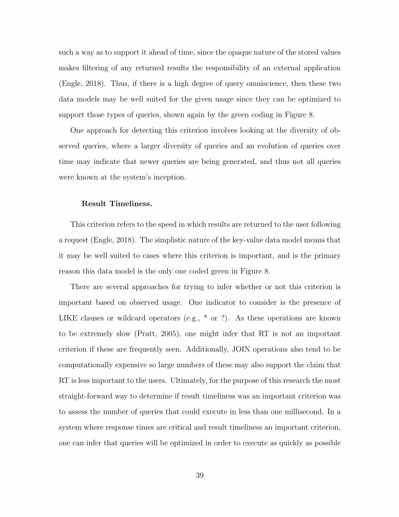
such a way as to support it ahead of time, since the opaque nature of the stored values

makes filtering of any returned results the responsibility of an external application

(Engle, 2018). Thus, if there is a high degree of query omniscience, then these two

data models may be well suited for the given usage since they can be optimized to

support those types of queries, shown again by the green coding in Figure 8.

One approach for detecting this criterion involves looking at the diversity of ob-

served queries, where a larger diversity of queries and an evolution of queries over

time may indicate that newer queries are being generated, and thus not all queries

were known at the system’s inception.

Result Timeliness.

This criterion refers to the speed in which results are returned to the user following

a request (Engle, 2018). The simplistic nature of the key-value data model means that

it may be well suited to cases where this criterion is important, and is the primary

reason this data model is the only one coded green in Figure 8.

There are several approaches for trying to infer whether or not this criterion is

important based on observed usage. One indicator to consider is the presence of

LIKE clauses or wildcard operators (e.g., * or ?). As these operations are known

to be extremely slow (Pratt, 2005), one might infer that RT is not an important

criterion if these are frequently seen. Additionally, JOIN operations also tend to be

computationally expensive so large numbers of these may also support the claim that

RT is less important to the users. Ultimately, for the purpose of this research the most

straight-forward way to determine if result timeliness was an important criterion was

to assess the number of queries that could execute in less than one millisecond. In a

system where response times are critical and result timeliness an important criterion,

one can infer that queries will be optimized in order to execute as quickly as possible

39

so a higher prevalence of them would indicate that this criterion is important.

2.6 Multi-Criteria Decision-Making

The foundational research discussed in the “Engle Criteria” section used inputs

from system Subject Matter Experts in order to produce a decision support aid for

selecting an appropriate data model, via an MCDM known as the Analytic Hierar-

chy Process (AHP). As a follow-on to the previous study, this research intended to

demonstrate the feasibility of producing a similar decision support model, however,

in lieu of SME inputs it instead was based on observations of an existing system.

Thus, a different approach for employing Engle’s AHP-based priorities through an

alternative multi-criteria decision-making model was pursued.

The Simple Additive Weighting (SAW) method is one of the best known (and

therefore, widely used) MCDM methods (Yoon & Hwang, 1995). Due to its ability

to improve quality and speed in decision-making, SAW has been widely applied to

diverse problem sets such as assigning percentage increases to employee raises, hiring

decisions for employees, and determining student admissions in vocational schools

(Afshari et al., 2010; Sahir et al., 2017; Wijayanto et al., 2019).

In SAW, alternative outcomes are calculated by multiplying a weight for a given

criteria against that alternative’s scoring for that criteria and then summing across the

results for each criteria (Yoon & Hwang, 1995). As an extremely simplistic example,

suppose a person is trying to decide which of two cars to purchase based on two

(normalized) criteria, cost, and speed. Cost is considered twice as important as speed,

so its weight is .666 compared to speed’s .333. Car A can reach a top speed of 55 mph

while Car B can reach a speed of 80 mph, and since a larger value is desirable here

their normalized values are found using a linear sum benefit criteria method (Vafaei

et al., 2016). Thus, for Car A its normalized speed value is given by the equation

40

(55)/(55 + 80) = 0.407 and Car B’s speed value is given by (80)/(55 + 80) = 0.593.

Regarding costs, Car A’s cost is $6,000 and Car B’s cost is $8,000. Since a smaller

value for cost is preferable, the normalized values are found using a linear sum cost

criteria method (Vafaei et al., 2016). Thus, Car A’s normalized cost value is given

by the equation ((1/6000)/((1/6000) + (1/8000))) = 0.571 and Car B’s cost value is

given by the equation ((1/8000)/((1/6000) + (1/8000))) = 0.429. Using SAW, the

value of Car A is computed as (0.571)(0.666) + (0.407)(0.333) = 0.516. Similarly,

Car B is computed as (0.429)(0.666) + (0.593)(0.333) = 0.484. Therefore, Car A is a

slightly better choice given these options.

Previous research has demonstrated the joint application of AHP and SAW in

order to make decisions using the AHP method to generate the initial weights, and

then leveraging the SAW method to determine the ranking of criteria (Wijayanto

et al., 2019). A similar approach is used here. In this research, Engle’s performance

priorities serve as the foundation for the SAW weighting while the observations of

actual database usage will provide the normalized scoring values for each criterion.

Collectively, these efforts yield an effective objective methodology for selecting alter-

native NoSQL data models for a given observed use case. A more thorough treatment

of this approach will be discussed in the next chapter.

2.7 Conclusion

The purpose of this chapter was to review the trends in database storage models

beginning with the relational data model of the 1970’s through the emergence of

today’s Big Data-driven NoSQL data models. The characteristics and strengths of

these data models make them attractive candidates for use in several interesting use

cases. Existing research that studied ways of characterizing the usage of a relational

database was also discussed.

41

That treatment served as the foundation for the next discussion, which will

introduce a novel approach towards characterizing the usage of existing relational

databases in an automated fashion in order to assess the suitability of various NoSQL

data models within the context of an existing relational database system. The fol-

lowing chapter discusses the proposed approach towards satisfying this objective and

demonstrates its usage through an exemplary pilot study.

42

III. Methodology

3.1 Research Design

In prior research conducted by Engle (Engle, 2018), a set of twelve criteria (termed

the “Engle criteria”) were defined that collectively can be used to assess the suitability

of a given data model based on a user’s subjective assessments of how important each

of those criteria are (relative to one another) for a particular system and use case

under consideration. This research built upon his work by extending the approach

with a novel methodology utilizing objective measurements of the system’s usage in

lieu of subjective assessments from system users.

Several steps were required in order to implement this methodology. First, a tool

(called “Engle Criteria Analysis Tool” or ECAT) was developed which passively ob-

serves interactions between a user or application and a relational database in order

to infer the degree to which the observed traffic contains elements of the Engle crite-

ria. Second, a series of simulations based on real-world use cases were constructed to

demonstrate the tool against different types of usage profiles and to generate obser-

vations. Finally, the observations were used to generate relative weights, which were

then employed in a Simple Additive Weighting decision model to provide insights

regarding the suitability of alternative NoSQL data models for the observed use cases

by producing a rank-ordered list of suggested data models.

3.2 Research Questions & Hypotheses

In order to guide this research, a number of research questions and hypotheses

were considered.

43

Mapping of Research Questions to Methodology.

The research questions introduced in Chapter 1 are repeated again in Table 4 for

ease of reference, along with a mapping of the methods used towards answering each

of the questions. Both of the questions rely upon a simulation study described in

the following section which was employed to identify suitable features in the observed

data. These features were measured to produce the weighting of the Engle criteria for

use in the SAW decision model for mapping the observed usage to the most suitable

underlying data models.

Table 4. Research Questions and Associated Research Methodologies

Research Questions Sim

ula

tion

Deci

sion

Model

1. Which observable criteria exist for assessing the usage patterns of a non-distributed relational database in an automated fashion?

X X

2. Using an automated methodology, can non-distributed relational databaseusage patterns be mapped to more suitable data models using the observablecriteria?

X X

Hypotheses.

In order to support answering the stated research questions, this research sought

to answer the following three hypotheses:

1. One or more elements of the Engle criteria can be mapped to observable char-

acteristics of relational database systems.



44




Regarding the first hypothesis, the Engle criteria has already been shown to be

useful for the selection of an appropriate data model in a single-box environment

(Engle, 2018). However, to date these criteria have only been applied to notional

database systems with the assistance of inputs from system SMEs. This research

proposed a different approach to investigate the use of the Engle criteria in an au-

tomated fashion by considering if there were observable characteristics of relational

database systems that might inform or “map” back to the various Engle criteria.

Testing this hypothesis involved demonstrating whether or not this mapping could

be accomplished.

Assuming the first hypothesis could be satisfied, then one or more characteristics

of a relational database system can be observed which are able to be mapped to the

Engle criteria. The second hypothesis posits that there is sufficient evidence provided

by these observable characteristics such that it is possible to quantitatively profile the

aggregate usage patterns (in terms of the Engle criteria) of the users of a relational

database system.

Finally, the third hypothesis builds on the previous two by assuming that if there

are enough observable characteristics in order to develop quantitative profiles of re-

lational database users, then these observations could then be used to categorize and

rank the suitability of the NoSQL data models for the observed usage.

3.3 Instrumentation

In order to develop the instrumentation for this research, an initial pilot study was

undertaken into the original 12 Engle criteria (Engle, 2018), which were introduced

45

in the previous chapter. This pilot study was built upon an open-source database

called “Classicmodels” (which will be discussed in greater detail in Sections 3.7 and

3.8). The purpose of the pilot study was to serve as a test bed where each of the

criteria could be studied and considered in order to determine under what potential

circumstances these criteria could be observed through observation of SQL queries

from a system of interest, as well as to demonstrate the feasibility of this approach

and highlight potential issues that might be encountered during later research.

Based on this initial investigation, it was determined that 9 of the 12 criteria

could be partially or wholly observed, and these became candidates for implemen-

tation into the tool. One of the criteria, Pre-processing, relies solely on information

that is outside the observable scope of this work (i.e., it requires an understanding

of processing actions that take place on the data prior to its use in the relational

database); therefore, this criterion was not considered in this research. Addition-

ally, it was determined that while the necessary information for calculating the Large

Aggregate Transactions and Small Aggregate Transaction criteria does exist in the

observed data, no means of reliably extracting the aggregate sizes and relating them

back to the associated queries which generated the data were found during the course

of this study, and thus these two were also not implemented. The remaining criteria

were then developed into 9 individual functions in the ECAT software code, each as-

sessing one of the remaining criteria. The individual functions are discussed in more

detail later in this section. For the interested reader, the code that comprises ECAT

can be found in Appendix A.

System Design.

As an introduction to the high-level design of the system, consider Figure 9.

This graphic depicts the logical system setup including the users and/or applications

46

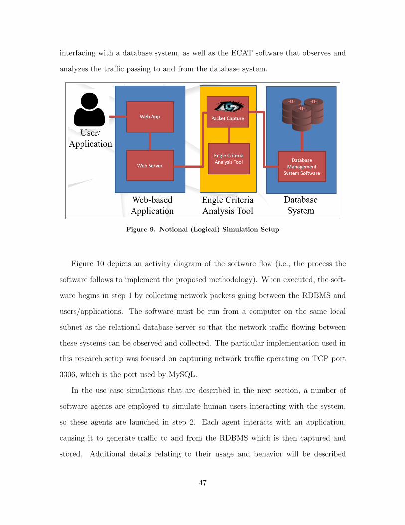
interfacing with a database system, as well as the ECAT software that observes and

analyzes the traffic passing to and from the database system.

Figure 9. Notional (Logical) Simulation Setup

Figure 10 depicts an activity diagram of the software flow (i.e., the process the

software follows to implement the proposed methodology). When executed, the soft-

ware begins in step 1 by collecting network packets going between the RDBMS and

users/applications. The software must be run from a computer on the same local

subnet as the relational database server so that the network traffic flowing between

these systems can be observed and collected. The particular implementation used in

this research setup was focused on capturing network traffic operating on TCP port

3306, which is the port used by MySQL.

In the use case simulations that are described in the next section, a number of

software agents are employed to simulate human users interacting with the system,

so these agents are launched in step 2. Each agent interacts with an application,

causing it to generate traffic to and from the RDBMS which is then captured and

stored. Additional details relating to their usage and behavior will be described

47

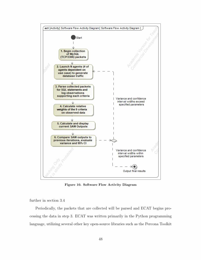
Figure 10. Software Flow Activity Diagram

further in section 3.4

Periodically, the packets that are collected will be parsed and ECAT begins pro-

cessing the data in step 3. ECAT was written primarily in the Python programming

language, utilizing several other key open-source libraries such as the Percona Toolkit

48

to help facilitate the distillation of observed traffic into individual SQL queries (Per-

cona, LLC., 2019). The Percona Toolkit was used here to assist in decoding the

MySQL packets and extracting the embedded SQL statements. After the SQL state-

ments are extracted, ECAT discards any SQL statements that do not provide useful

information about how the database is being used (e.g., “administrator command”,

“version()”, “set session sql mode”, etc.). Then, ECAT processes the remaining SQL

statements through the individual functions that each handle one of the nine Engle

criteria. The output from each of the functions is a count of the number of SQL

statements that provide support for the importance of the given criteria.

The counts for each of the SQL statements that support each criteria which were

generated in the previous step are then used in step 4 to calculate the relative weights

of each criteria. This is accomplished by summing across all of the observed state-

ments and then dividing each criterion by the total observed count.

Step 5 takes the relative counts for each of the criteria and cross multiplies them by

their associated performance priorities in order to build the Simple Additive Weight-

ing model, which defines the relative ranking for each of the data models based on

the data observed up to this point.

Finally, step 6 compares the output from the SAW model in step 5 to the outputs

from previous any periodic checks. In order to determine if a sufficient amount of data

has been collected, the variance of the four most recent rankings for each of the data

models is computed, as well as a confidence interval based on each of the iterations

seen thus far. A threshold of 1 × 10−5 is used to determine if the data model ranking

values are differing significantly from one iteration to the next. Additionally, the

width of the 95% confidence interval is also computed and inspected to determine if

it has fallen below .01. If either of these criteria have not yet been met, then the

process loops back to step 2 to continue generating observations.

49

Strategies for Observing the Engle Criteria.

After considering the Engle Criteria and analyzing the potential ways each of the

criteria could be detected or inferred from the observed database usage data, the best

identified approaches were written into the ECAT software. The following discussion

explains the strategies that were selected and implemented in ECAT for each of the

observable criteria.

Criterion 1 - Pre-Processing (N/A).

As previously mentioned, this criterion relies on information about processing that

occurs before data is entered into the RDBMS. As such, this criterion was deemed

unobservable. Therefore, it was not implemented in ECAT.

Criterion 2 - Structural Malleability.

This function is designed to provide evidences of RDBMS usage indicating that

the “DBMS’s ability to add/remove ‘types’ of aggregates to and from the DBMS” is

considered important (Engle, 2018). The primary strategy of this function is to look

for the presence of any “CREATE TABLE” or “DROP TABLE” commands since an

aggregate type in a normalized RDBMS would likely be implemented as a separate

table.

Furthermore, since it would be in a separate table, an “ALTER TABLE” command

updating a foreign key constraint would further support this criterion. However, if a

“RENAME TABLE” is observed following the “CREATE” or “ALTER” commands,

then they are not counted here but instead are counted later by the Plasticity criterion.

50

Criterion 3 - Transparency.


the “DBMS’s ability to store aggregates such that individual elements within the

aggregate can be viewed and retrieved during read transactions” (Engle, 2018). This

function evaluates queries to determine if “SELECT” statements are querying a subset

of the attributes for a given relation or if it is requesting all attributes.

Generally, one would request all attributes by using a “SELECT *” statement,

however it is possible to enumerate each attribute so this must also be accounted

for. This is done by comparing the list of attributes against the schema of the ta-

ble. Changes made to the schema during execution (i.e., through “ALTER TABLE”

commands) are identified and stored so that the current version of the schema is refer-

enced for any given query. Finally, when “JOINS” are present specific attributes may

be referenced using an alias and dot notation (e.g., a.col one, b.col two). Therefore,

this function also considers the possibility that multiple aggregates may be accessed

in a single statement, and it keeps track of the elements and whether or not all of

them are accessed across all specified relations or not.

Criterion 4 - Query Omniscience.

This function is designed to provide evidences of RDBMS usage indicating the

“degree to which the complete set of possible queries is known by the user before

(the) system is implemented” (Engle, 2018). This function takes a time-ordered list of

fingerprinted SQL queries that have been run against the database and then partitions

the list into three equal lists. The query fingerprints are sorted alphabetically, and

a similarity comparison is made between each of the three lists. The premise is

that if the usage of a database is homogeneous across the entire span of observed

usage, then each of the three subsets of queries should contain approximately the

51

same number of each type of query. By comparing each subset of lists to the others,

it can be determined whether or not the types of queries that were observed have

evolved or changed over time. Observing a change in usage over time may imply that

the complete set of possible queries was not determined by the users prior to system

implementation.

This comparison is performed using an implementation of the Jaccard distance

metric from the Python SciPy library (Jaccard, 1912; Virtanen et al., 2020). This

metric calculates the difference in terms of occurrences from one set to another, so

two lists that are completely identical will return a value of 1, whereas two completely

different lists will return a value of zero. By performing three pair-wise comparisons

on each of the three lists (i.e., comparing the first list to the second, the second list

to the third, and the first list to the third), three distance metrics are generated.

These metrics are then averaged together to get an overall difference score across the

entire set of observed queries. Lists that are homogeneous will return higher overall

scores, indicating a higher degree of query omniscience. Conversely, heterogeneous

lists will return low overall scores, indicating that a change in usage was likely during

the observed period.

Criterion 5 - Query Complexity.


“DBMS’s ability to perform both simple and complex queries” (Engle, 2018). Simple

queries are those in which the data is retrieved “using only a unique identifier or a

range of identifiers and/or values” (Engle, 2018), whereas more complex queries may

impose additional conditions or perform aggregation functions (e.g., sum, count, max,

etc.) on the results.

This function searches through the queries using string-matching techniques to

52

identify queries that are considered complex and then returns the value of the number

of complex queries observed since higher values of these indicate that this criterion is

important.

Criterion 6 - Result Timeliness.

This function is designed to provide evidences of RDBMS usage indicating “how

quickly the results are provided to the user after a request is made” (Engle, 2018).

This function leverages the Percona Toolkit to search for queries exceeding a spec-

ified threshold, which is specified to be one millisecond. The observation of a large

proportion of queries taking longer than this to run may imply that the user is less

concerned with this criterion; therefore, this value is subtracted from the total num-

ber of observed queries to produce the number of queries that ran quickly since higher

values denote that this criterion may be more important.

Criterion 7 - Cross-Aggregate Consistency.


“DBMS’s ability to perform cascading updates to data and relationships” (Engle,

2018). In a relational database, this can be observed through update or delete oper-

ations involving joins so this function employs string matching techniques to identify

these and returns a count of these queries since higher values indicate that this crite-

rion is important.

Criterion 8 - Large Transactions (N/A).


the “DB can store, retrieve, and update large (>1TB) aggregates quickly (within a

few seconds or less)” (Engle, 2018). Since the results from any query are observable

53

in the data, it should be possible to measure these results and obtain a count of

the number of large transactions being observed. However, at this time a means of

accurately extracting this information was not found and remains a goal for future

research. Should this data be obtained, higher occurrences of this criterion in the

observed usage would indicate that this criterion is important.

Criterion 9 - Small Transactions (N/A).


the “DB can store, retrieve, and update small (<1kB) aggregates quickly (within a

few seconds or less)” (Engle, 2018). As with the previous criterion, this information

also exists within the observed data; however, a means of extracting was not found.

Also as before, should this data be obtained, then higher occurrences of this criterion

in the observed usage would indicate that this criterion is important.

Criterion 10 - Plasticity.


“DBMS’s ability to add or remove elements within stored aggregates” (Engle, 2018).

Observing such elements in a relational database would be identified by the pres-

ence of “ALTER TABLE” commands that either “ADD” and/or “DROP” columns.

Therefore, this function returns a count of any such observed occurrences.

Criterion 11 - Data Typing Enforcement.

This function is designed to provide evidences of RDBMS usage indicating “DB

enforcement of data types during transactions. Data types may include floats, dou-

bles, Booleans, strings and others” (Engle, 2018). Relational databases restrict the

“types” of data that are permitted to be written into them which helps ensure the

54

consistency of the data. If this criterion is important to the user, it may manifest itself

through updates to the database’s schema as users seek to ensure the consistency of

their data in response to changing needs. Thus, this function looks for the presences

of “ALTER TABLE” commands that either “CHANGE” or “MODIFY” the schema

and returns a count of such occurrences.

Criterion 12 - Manipulation.

Finally, this last function is designed to provide evidences of RDBMS usage in-

dicating the “DBMS’s ability to update elements within stored aggregates indepen-

dently from other aggregates and elements” (Engle, 2018). This function’s strategy is

to evaluate any “UPDATE” queries and check whether or not the query is specifying

values for all elements in a given relation or only a subset of them. If the latter, then

such queries are counted since they indicate this criterion is important.

3.4 Simulation

This research employed a series of simulations in order to generate and collect data

representative of typical real-world relational database systems based on different

types of application systems and usage styles. The purpose of the simulation study

was to demonstrate that the Engle criteria discussed in Chapter 1 can be collected by

a system observing the usage of a relational database by a user/application, and then

use that information to determine if a more suitable data model would be appropriate

for the given use case.

As pictured in Figure 9, the “Engle Criteria Analysis Tool” acted as a “man-in-

the-middle” between a user/application and a relational database system. Given its

placement, this tool was able to observe all queries sent to the database system, as

well as the responses from the database system. This allowed it to log all activity

55

which was then analyzed in order to produce metrics about the usage characteristics

of the database system for the given use case in the following simulations. This in

turn formed the basis for determining the weights for the decision model discussed in

the next section.

Inputs to the simulation were controlled by programmed agents, which are pieces

of software that were designed and constructed to interact with several different ap-

plications. Their purposes are to simulate the usage styles of human operators inter-

facing with these applications. These agents acted as the user in Figure 9. Different

parameters for each of the agents were adjusted to vary aspects of their interactions,

such as the frequency of which functions of the web application they were accessing.

This provided for the evaluation of different types of use cases for each of the eval-

uated systems. The output from the collected samples produced a packet capture

containing all network traffic between the relational database and the application,

which could be parsed to produce an ordered list of SQL queries and other related

metadata. These data were subsequently assessed by the ECAT tool discussed in the

previous section.

Several different use cases have been implemented in order to demonstrate a di-

verse selection of possible database uses in these simulations. These simulations

leveraged open-source software implementing real-world web applications such as an

online forum system, an authoritative Domain Name System (DNS) server, and a

social-networking website. All of these applications leverage the open-source MySQL

RDBMS as their back-end database, and each was chosen because of their support

for this particular RDBMS implementation. It should be noted, however, that the

principles of this research are intended to be implementation-agnostic and would ap-

ply to other types of RDBMS implementations given the proper changes to system

setup (such as adjusting the code to interpret other protocols beyond MySQL).

56

For the online forum system, phpBB was selected. PowerDNS was chosen for

the authoritative DNS server use case. Finally, Elgg was selected to represent a

social network use case. In each use case (i.e., phpBB, PowerDNS, and Elgg), agents

were run against the particular web application (or DNS service), prompting that

web application (or DNS service) to execute SQL queries to the RDBMS via TCP

port 3306 in order to satisfy the data requirements being generated by the agents’

actions. The traffic exchanged between the two hosts using the MySQL protocol is

unencrypted, which allows for the SQL queries and responses to be easily collected.

Since the systems being simulated reside on the same subnet, traffic passing be-

tween the two hosts can be “sniffed” using the tcpdump packet capture software which

resides on the ECAT host running on the same subnet. As the system collecting and

analyzing the data operates passively, it does not impact the data collection of the

system. Following the data collection, the data is parsed and analyzed by ECAT in

order to extract features of the observed data that can compute quantitative metrics

for each of the criteria presented in Table 1 and as discussed in Section 3.3.

Figure 11 shows a sample packet capture from the phpBB web application for the

following SQL query: “SELECT p.post id FROM phpbb posts WHERE p.topic id =

1 AND (p.post visibility = 1) ORDER BY p.post time ASC, p.post ID ASC LIMIT

10”. To demonstrate how this information could be used to inform one of the Engle

criterion, consider the query complexity criterion which measures the importance of

being able to perform complex queries in addition to simple ones. The query in this

example not only retrieves the desired data through a combination of two selection

parameters (p.topic id = 1 and p.post visibility = 1), but it also limits the results

based on a sorted subset of the data. This would indicate a non-trivial amount of

query complexity. Thus, this query would lend support for the importance of the

query the query complexity criteria and be counted in this metric. A high ranking

57

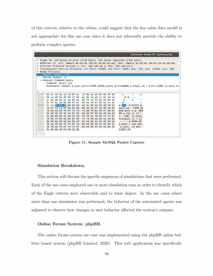
of this criteria, relative to the others, could suggest that the key-value data model is

not appropriate for this use case since it does not inherently provide the ability to

perform complex queries.

Figure 11. Sample MySQL Packet Capture

Simulation Breakdown.

This section will discuss the specific sequences of simulations that were performed.

Each of the use cases employed one or more simulation runs in order to identify which

of the Engle criteria were observable and to what degree. In the use cases where

more than one simulation was performed, the behavior of the automated agents was

adjusted to observe how changes in user behavior affected the system’s outputs.

Online Forum System: phpBB.

The online forum system use case was implemented using the phpBB online bul-

letin board system (phpBB Limited, 2020). This web application was specifically

58

chosen for this research for several reasons:

• It is open-source (thus it lacks licensing costs while also providing the ability to

modify it as required for any simulation/testing)

• It supports MySQL as a back-end database by default so its queries are com-

patible with the ECAT software

• The nature of online forum systems aligns with several characteristics of the

document or column-oriented NoSQL data models (e.g., containing lots of dy-

namically changing semi-structured or unstructured data) (Sadalage & Fowler,

2013)

Online forum systems such as this typically involve groups of users having conver-

sations with one another in the form of posted messages. As such, the agents for this

use case have each been programmed to replicate this behavior by use of the following

functions:

• Administrative actions (e.g., logging in and out)

• Select an available sub-forum, and enter it

• Create a new discussion thread

• Select an existing discussion thread, and enter it

• Create a new comment on an existing discussion thread

Generally, online forum systems have more read operations performed upon them

than write operations. A 2004 study of user behavior in university online forums

found that the average ratio of views to posts was 47.6:1 (Burr & Spennemann,

2004). Thus, the simulation setup adjusted the agents’ behavior to follow similar

59

parameters, with agents programmed to employ read functions (reading sub-forums

or discussion threads) 98 times out of 100, and write (create new discussion topics or

comments) the remaining two.

The behavior for each of the individual agents was adjusted stochastically during

execution. Each time an agent was instantiated, a specific percentage was assigned

to each of the read and write functions which the agent used for the duration of that

run. Each run involved the agent logging in and then performing approximately 30

user actions (pseudo-randomly chosen from a range of 20-40 actions for each run)

from the available options: accessing an existing sub-forum (15% − 20%), creating a

new discussion thread (1%−3%), reading an existing discussion thread (75%−80%),

or creating a new comment on an existing thread (1% − 3%). The agent would then

log out. Each agent performed this sequence repeatedly until a sufficient amount of

data had been collected.

The aforementioned user behavior study also highlighted different access patterns

throughout the day and week during an academic semester. These patterns could

also have been programmed into the agent’s behavior to increase the level of realism

in the simulation. The study indicated that their university supported nearly 40,000

students, and their data collection encompassed 589, 359 posts and 28, 025, 746 views

over a three-year period (Burr & Spennemann, 2004). As a three-year simulation for

this study was not feasible, agents were instead programmed to operate as quickly

as the overall simulation permits. Since most of the overhead was on the client side

(i.e., launching and operating a graphical web browser), multiple agent systems were

launched simultaneously in order to speed up data collection.

At periodic intervals, the ECAT software was run against the packets collected

thus far to monitor the results. Eventually, the SAW output results began to con-

verge to the desired level of fidelity (three decimal places), and the simulation was

60

terminated.

Authoritative Domain Name System: PowerDNS.

The authoritative PowerDNS domain name system was deliberately chosen for

this research to demonstrate a simple use case with only one possible agent action:

• Querying a domain

As with the previous use case, PowerDNS was chosen as a use case for this re-

search among a variety of options, because it is open-source and supports MySQL.

Additionally, the simplistic nature of this use case mirrored a common design feature

for the key-value NoSQL data type, namely that you provide the application with a

hostname (i.e., a key), and it returns the associated DNS information (i.e., a value).

As this was an authoritative DNS server, it provided only lookup capabilities for the

entries stored in its database (as opposed to a recursive DNS server whose function is

to forward DNS queries to the appropriate authoritative DNS servers). The lookup

queries were performed directly from Python using the built-in socket library.

Social Networking Site: Elgg.

Finally, the most complex use case was the Elgg social networking site. As was the

case with the previous use cases, it too was built using open-source software, and it

utilizes MySQL for its back-end database. Additionally, at first glance the Elgg social

networking site use case bears a resemblance to the phpBB online forum system as

both are primarily concerned with agents interacting with a website in order to read

and create content. However, looking beyond this superficial similarity reveals a key

difference between how these systems operate; namely, there is a rigid hierarchical

structure in the online forum system that is not present in the social networking

use case. Instead, the focus is on highly interconnected data as users create posts

61

that do not follow hierarchical structures and create ad hoc links between each other.

Therefore, the following functions were created for the agent supporting this use case:

• Administrative actions (e.g., logging in and out, creating new users)

• Becoming friends with a random user

• Reading a page (similar to viewing a thread of comments on a Facebook post)

• Creating a new page (similar to a new post on Facebook)

• Creating a comment on a page (similar to a comment on a post on Facebook)

• Retrieving a list of friends for a given user

As with the online forum system, ten agents were programmed to simultaneously

interact with the social networking site following a less “academic” style of posting.

That is, there was more emphasis on adding comments and content as might be

expected on a more “social” platform. Each agent was programmed to log in, and

pseudo-randomly perform 20 actions from the available options: becoming friends

with a new user (4% − 6%), reading a user’s profile (7% − 13%), reading a page

(25% − 35%), retrieving a list of friends for a pseudo-randomly user (7% − 13%),

comment on another user’s post (25%−35%), or create a new page (7%−13%). The

agent would then log out.

As before, the simulation was checked periodically and the packet capture pro-

cessed by ECAT to determine when the SAW output results started to converge. At

that point, the simulation was terminated.

3.5 Data Analysis - Calculating Relative Weights

Once the simulation data had been acquired, the next step was to calculate the

relative weights of the nine criteria based on their observed prevalence during a par-

62

ticular use case. It may be noted that this data was also calculated and periodically

updated during the data collection phases between packet captures in order to deter-

mine how long to allow the simulations to run. However, this discussion will focus on

the final output that was run against the entirety of the collected data.

To simplify this discussion, an example of how the collected metrics were calcu-

lated utilizing three of the nine Engle criteria (Cross-Aggregate Consistency (CAC),

Plasticity (Pla), and Query Complexity (QC)) is offered. We assume the number

of observations for each criterion has been captured during a simulation, along with

a count of the total number of observed queries for the entire simulation. In this

hypothetical example, we observed 500 SQL queries and evaluated them according to

the criteria discussed in Section 3.3.

Cross-Aggregate Consistency is evaluated based on operations that affect multiple

rows of data. For this example, assume that 50 of the 500 queries made adjustments

to results across more than one table. Therefore, the relative count for CAC is 50.

Plasticity is evaluated based on queries containing “ALTER TABLE” statements

which add or remove attributes in an existing table. For this example, assume that 5 of

the 500 queries made adjustments of this kind during the observed usage. Therefore,

the relative count for Pla is 5.

Query Complexity is evaluated based on the ratio of queries that are not based

on simple lookups (e.g., they contain a complex operation such as JOIN, LIKE,

SUM, etc.). For this example, assume that 250 of the 500 queries contained complex

operators. Therefore, the relative count for QC is 250.

Summing over the criteria gives a total of: 50 + 5 + 250 = 305.

To compute their relative weights, each is now divided by the total observed

cases. For CAC, the relative weight is 50/305 = .164. For Pla, the relative weight is

5/305 = .016. Finally, for QC the relative weight is 250/305 = .820. These normalized

63

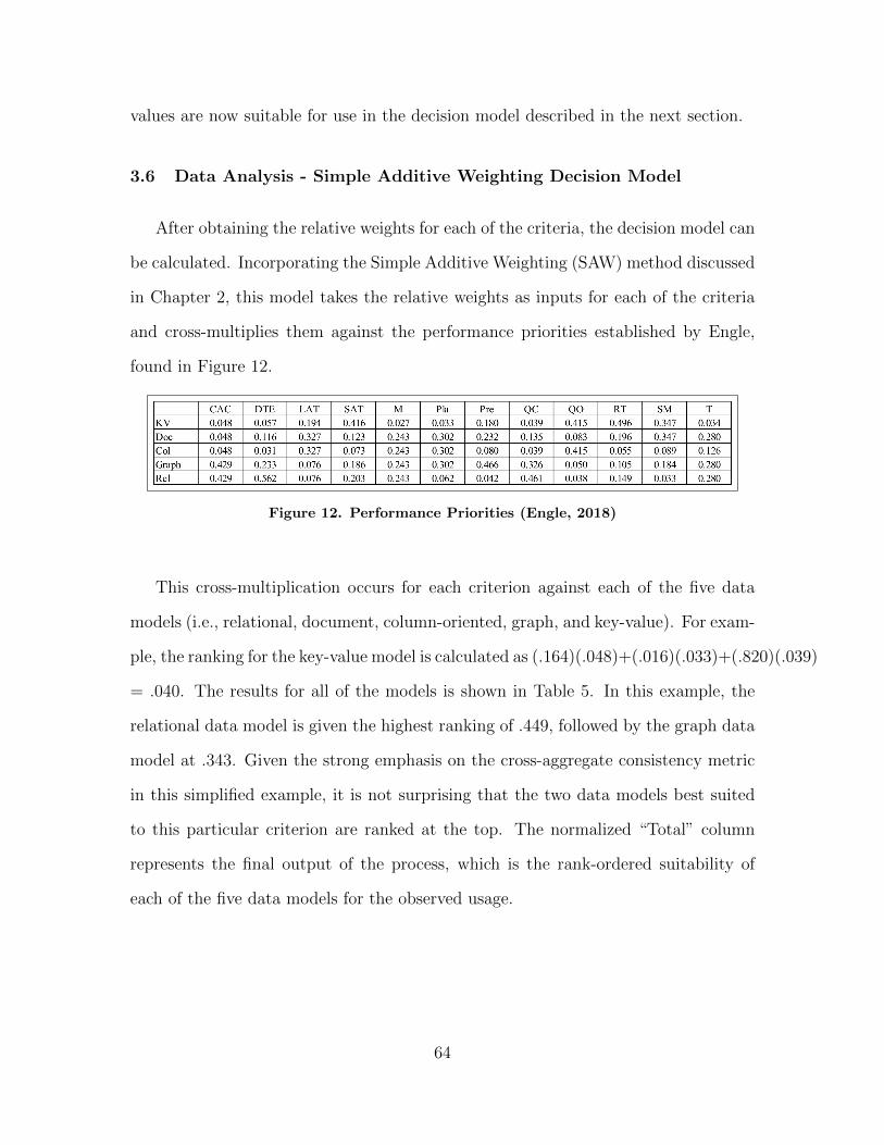
values are now suitable for use in the decision model described in the next section.

3.6 Data Analysis - Simple Additive Weighting Decision Model

After obtaining the relative weights for each of the criteria, the decision model can

be calculated. Incorporating the Simple Additive Weighting (SAW) method discussed

in Chapter 2, this model takes the relative weights as inputs for each of the criteria

and cross-multiplies them against the performance priorities established by Engle,

found in Figure 12.

Figure 12. Performance Priorities (Engle, 2018)

This cross-multiplication occurs for each criterion against each of the five data

models (i.e., relational, document, column-oriented, graph, and key-value). For exam-

ple, the ranking for the key-value model is calculated as (.164)(.048)+(.016)(.033)+(.820)(.039)

= .040. The results for all of the models is shown in Table 5. In this example, the

relational data model is given the highest ranking of .449, followed by the graph data

model at .343. Given the strong emphasis on the cross-aggregate consistency metric

in this simplified example, it is not surprising that the two data models best suited

to this particular criterion are ranked at the top. The normalized “Total” column

represents the final output of the process, which is the rank-ordered suitability of

each of the five data models for the observed usage.

64

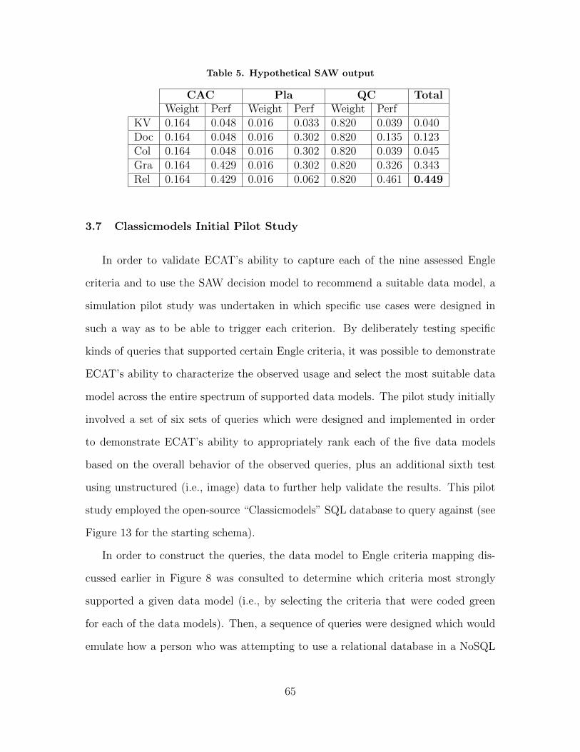
Table 5. Hypothetical SAW output

CAC Pla QC TotalWeight Perf Weight Perf Weight Perf

KV 0.164 0.048 0.016 0.033 0.820 0.039 0.040Doc 0.164 0.048 0.016 0.302 0.820 0.135 0.123Col 0.164 0.048 0.016 0.302 0.820 0.039 0.045Gra 0.164 0.429 0.016 0.302 0.820 0.326 0.343Rel 0.164 0.429 0.016 0.062 0.820 0.461 0.449

3.7 Classicmodels Initial Pilot Study

In order to validate ECAT’s ability to capture each of the nine assessed Engle

criteria and to use the SAW decision model to recommend a suitable data model, a

simulation pilot study was undertaken in which specific use cases were designed in

such a way as to be able to trigger each criterion. By deliberately testing specific

kinds of queries that supported certain Engle criteria, it was possible to demonstrate

ECAT’s ability to characterize the observed usage and select the most suitable data

model across the entire spectrum of supported data models. The pilot study initially

involved a set of six sets of queries which were designed and implemented in order

to demonstrate ECAT’s ability to appropriately rank each of the five data models

based on the overall behavior of the observed queries, plus an additional sixth test

using unstructured (i.e., image) data to further help validate the results. This pilot

study employed the open-source “Classicmodels” SQL database to query against (see

Figure 13 for the starting schema).

In order to construct the queries, the data model to Engle criteria mapping dis-

cussed earlier in Figure 8 was consulted to determine which criteria most strongly

supported a given data model (i.e., by selecting the criteria that were coded green

for each of the data models). Then, a sequence of queries were designed which would

emulate how a person who was attempting to use a relational database in a NoSQL

65

Figure 13. Initial Classicmodels Schema (mysqltutorial.org, 2020)

data model style might do so. The following sections discuss the approaches that

were taken with each of the simulations.

Classicmodels Simulation #1: Relational.

In the first simulation of the pilot study, a single agent was launched to interact

with the MySQL database which generated 264 observed queries. During the simu-

lation, 156 queries were retained for analysis, and 108 queries were omitted by the

ECAT tool. Regarding the 108 omitted queries, ECAT was programmed to disregard

queries which do not provide any useful information towards profiling the usage pat-

terns (such as “COMMIT” statements, or administrative commands such as connect

or ping). The queries of interest that were retained included but were not limited to

66

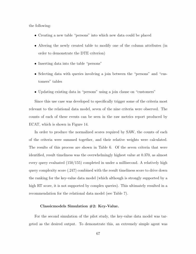
the following:

• Creating a new table “persons” into which new data could be placed

• Altering the newly created table to modify one of the column attributes (in

order to demonstrate the DTE criterion)

• Inserting data into the table “persons”

• Selecting data with queries involving a join between the “persons” and “cus-

tomers” tables

• Updating existing data in “persons” using a join clause on “customers”

Since this use case was developed to specifically trigger some of the criteria most

relevant to the relational data model, seven of the nine criteria were observed. The

counts of each of these events can be seen in the raw metrics report produced by

ECAT, which is shown in Figure 14.

In order to produce the normalized scores required by SAW, the counts of each

of the criteria were summed together, and their relative weights were calculated.

The results of this process are shown in Table 6. Of the seven criteria that were

identified, result timeliness was the overwhelmingly highest value at 0.370, as almost

every query evaluated (150/155) completed in under a millisecond. A relatively high

query complexity score (.247) combined with the result timeliness score to drive down

the ranking for the key-value data model (which although is strongly supported by a

high RT score, it is not supported by complex queries). This ultimately resulted in a

recommendation for the relational data model (see Table 7).

Classicmodels Simulation #2: Key-Value.

For the second simulation of the pilot study, the key-value data model was tar-

geted as the desired output. To demonstrate this, an extremely simple agent was

67

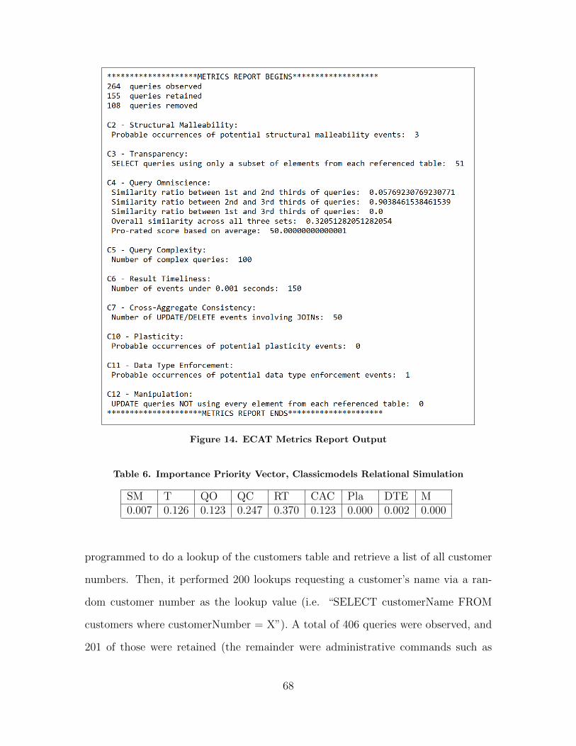
Figure 14. ECAT Metrics Report Output

Table 6. Importance Priority Vector, Classicmodels Relational Simulation

SM T QO QC RT CAC Pla DTE M0.007 0.126 0.123 0.247 0.370 0.123 0.000 0.002 0.000

programmed to do a lookup of the customers table and retrieve a list of all customer

numbers. Then, it performed 200 lookups requesting a customer’s name via a ran-

dom customer number as the lookup value (i.e. “SELECT customerName FROM

customers where customerNumber = X”). A total of 406 queries were observed, and

201 of those were retained (the remainder were administrative commands such as

68

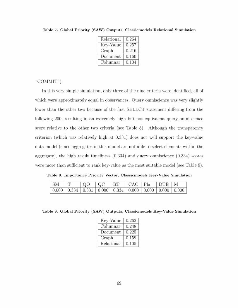
Table 7. Global Priority (SAW) Outputs, Classicmodels Relational Simulation

Relational 0.264Key-Value 0.257Graph 0.216Document 0.160Columnar 0.104

“COMMIT”).

In this very simple simulation, only three of the nine criteria were identified, all of

which were approximately equal in observances. Query omniscience was very slightly

lower than the other two because of the first SELECT statement differing from the

following 200, resulting in an extremely high but not equivalent query omniscience

score relative to the other two criteria (see Table 8). Although the transparency

criterion (which was relatively high at 0.331) does not well support the key-value

data model (since aggregates in this model are not able to select elements within the

aggregate), the high result timeliness (0.334) and query omniscience (0.334) scores

were more than sufficient to rank key-value as the most suitable model (see Table 9).

Table 8. Importance Priority Vector, Classicmodels Key-Value Simulation


Table 9. Global Priority (SAW) Outputs, Classicmodels Key-Value Simulation

Key-Value 0.262Columnar 0.248Document 0.225Graph 0.159Relational 0.105

69

Classicmodels Simulation #3: Columnar.

In the third simulation of the pilot study, the columnar data model was targeted

as the intended output from ECAT. This was done by executing a number of queries

to modify a table by adding and removing columns in order to trigger manipulation,

and by keeping the types of commands observed consistent (i.e., the same types were

observed in the beginning as at the end) in order to support query omniscience since

these two criteria predominantly support this data model.

Table 10. Importance Priority Vector, Classicmodels Columnnar Simulation


Of the five criteria that were identified, manipulation (0.334) and query omni-

science (0.331) ended up being the dominating values (see Table 10). As intended,

these factors combined heavily supported the columnar data model, which was the

highest ranked as seen in Table 11.

Table 11. Global Priority (SAW) Outputs, Classicmodels Columnar Simulation

Columnar 0.292Key-Value 0.209Document 0.198Graph 0.177Relational 0.124

Classicmodels Simulation #4: Graph.

The fourth simulation of the pilot study targeted the graph data model. Sev-

eral key strengths of the graph data model are the ability to update values across

aggregates (Cross-Aggregate Consistency), to add or remove elements within stored

70

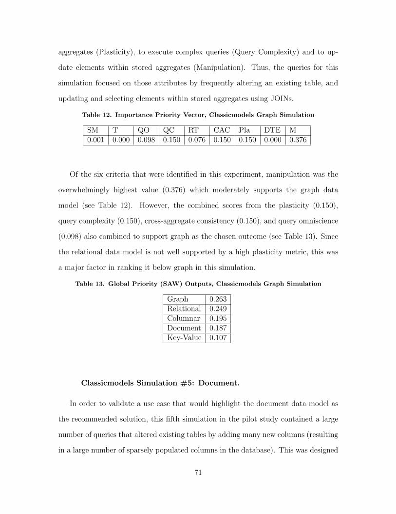
aggregates (Plasticity), to execute complex queries (Query Complexity) and to up-

date elements within stored aggregates (Manipulation). Thus, the queries for this

simulation focused on those attributes by frequently altering an existing table, and

updating and selecting elements within stored aggregates using JOINs.

Table 12. Importance Priority Vector, Classicmodels Graph Simulation


Of the six criteria that were identified in this experiment, manipulation was the

overwhelmingly highest value (0.376) which moderately supports the graph data

model (see Table 12). However, the combined scores from the plasticity (0.150),

query complexity (0.150), cross-aggregate consistency (0.150), and query omniscience

(0.098) also combined to support graph as the chosen outcome (see Table 13). Since

the relational data model is not well supported by a high plasticity metric, this was

a major factor in ranking it below graph in this simulation.

Table 13. Global Priority (SAW) Outputs, Classicmodels Graph Simulation

Graph 0.263Relational 0.249Columnar 0.195Document 0.187Key-Value 0.107

Classicmodels Simulation #5: Document.

In order to validate a use case that would highlight the document data model as

the recommended solution, this fifth simulation in the pilot study contained a large

number of queries that altered existing tables by adding many new columns (resulting

in a large number of sparsely populated columns in the database). This was designed

71

to mimic the type of schemaless behavior that would be expected when employing

the document data model, typified by high values for the plasticity and structural

malleability criteria.

Table 14. Importance Priority Vector, Classicmodels Document Simulation


Of the five criteria that were identified, plasticity was the overwhelmingly highest

value (0.717), followed by a value of 0.140 for structural malleability (see Table 14).

These two factors combined heavily support the document data model (see Table 15).

Table 15. Global Priority (SAW) Outputs, Classicmodels Document Simulation

Document 0.294Graph 0.272Columnar 0.239Key-Value 0.110Relational 0.086

Classicmodels Simulation #6: Unstructured data.

As a capstone simulation in the initial pilot study, an agent was programmed to

insert and query large amounts of unstructured data (in the form of base64-encoded

jpeg images) in order to demonstrate their impact on a relational database. A total

of 80 images were inserted (at approximately 3-4Mb each), and then 25 of them were

randomly read back out in order to perform this test.

Table 16. Importance Priority Vector, Classicmodels Unstructured Data Simulation


72

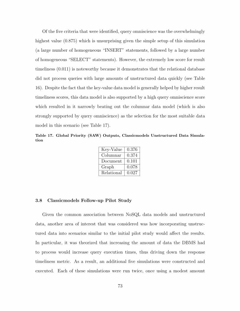
Of the five criteria that were identified, query omniscience was the overwhelmingly

highest value (0.875) which is unsurprising given the simple setup of this simulation

(a large number of homogeneous “INSERT” statements, followed by a large number

of homogeneous “SELECT” statements). However, the extremely low score for result

timeliness (0.011) is noteworthy because it demonstrates that the relational database

did not process queries with large amounts of unstructured data quickly (see Table

16). Despite the fact that the key-value data model is generally helped by higher result

timeliness scores, this data model is also supported by a high query omniscience score

which resulted in it narrowly beating out the columnar data model (which is also

strongly supported by query omniscience) as the selection for the most suitable data

model in this scenario (see Table 17).

Table 17. Global Priority (SAW) Outputs, Classicmodels Unstructured Data Simula-tion

Key-Value 0.376Columnar 0.374Document 0.101Graph 0.078Relational 0.027

3.8 Classicmodels Follow-up Pilot Study

Given the common association between NoSQL data models and unstructured

data, another area of interest that was considered was how incorporating unstruc-

tured data into scenarios similar to the initial pilot study would affect the results.

In particular, it was theorized that increasing the amount of data the DBMS had

to process would increase query execution times, thus driving down the response

timeliness metric. As a result, an additional five simulations were constructed and

executed. Each of these simulations were run twice, once using a modest amount

73

of unstructured data (approximately 30 kilobytes) and then again using a larger

amount of unstructured data (approximately 500 kilobytes). One primary interest

of this follow-up study was to determine the impact of using such variable amounts

of unstructured data on the result timeliness criterion. The code used to run these

follow-up simulations can be found in Appendix B.

Classicmodels Follow-up Simulation #1: Relational with Unstruc-

tured Data.

This simulation’s setup largely followed the setup from the relational simulation

in the initial pilot study; however, an additional attribute was added to the table

to hold the unstructured data. This field was created as a “LONGBLOB”, a data

type designed for storing binary strings (such as a picture file). Table 18 shows the

impact of changing the average file size between the two runs. The dramatic decrease

in value for result timeliness (from 0.415 to 0.300) allowed for increases in the other

criteria.

Table 18. Importance Priority Vector, Classicmodels Follow-Up Simulation, Relationalwith Unstructured Data

SM T QO QC RT CAC Pla DTE M∼30kb 0.003 0.210 0.058 0.208 0.415 0.000 0.000 0.002 0.104∼500kb 0.004 0.249 0.071 0.248 0.300 0.000 0.000 0.002 0.125

The corresponding effect on the global priorities for this shift can then be observed

in Table 19. The impact of the increased amount of data resulted in a shift in the

overall highest ranked data models. When only a small amount of unstructured

data was handled by ECAT, the key-value (0.249) data model was selected as the

most suitable, followed closely by relational (0.245). However, when larger amounts

of data were included, key-value (0.202) fell to third, after relational (0.264) and

graph (0.217). This finding is somewhat counter-intuitive, since one of the strengths

74

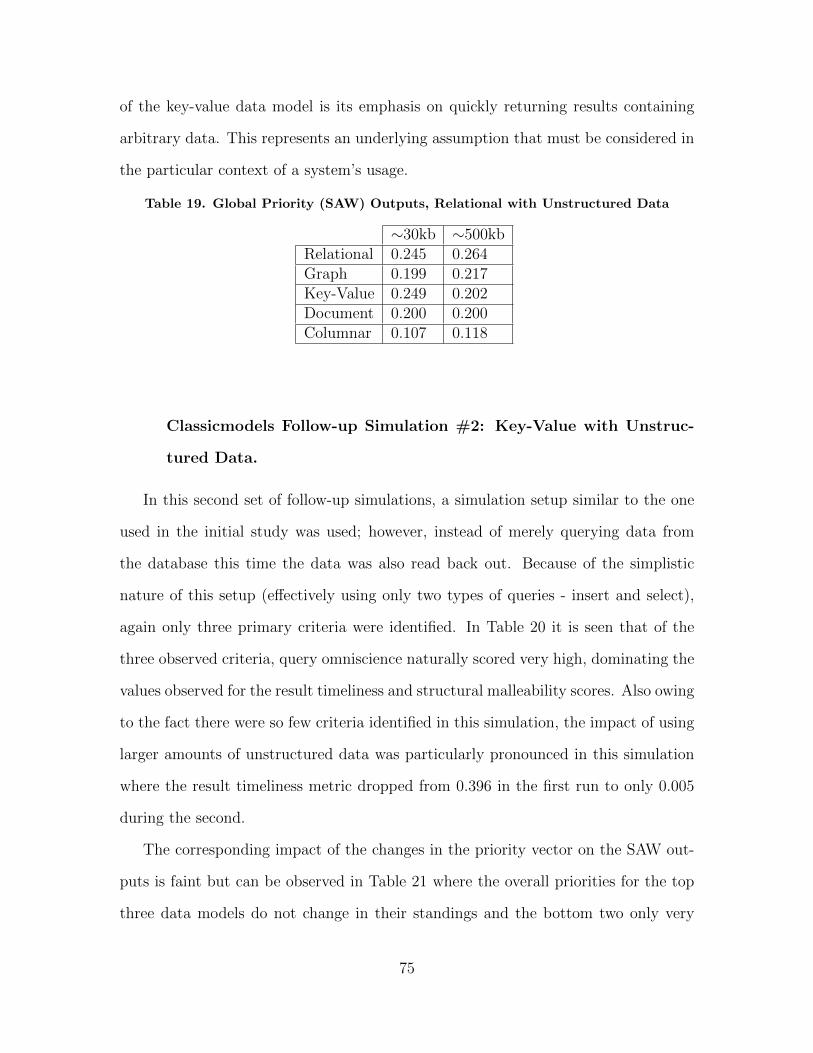
of the key-value data model is its emphasis on quickly returning results containing

arbitrary data. This represents an underlying assumption that must be considered in

the particular context of a system’s usage.

Table 19. Global Priority (SAW) Outputs, Relational with Unstructured Data

∼30kb ∼500kbRelational 0.245 0.264Graph 0.199 0.217Key-Value 0.249 0.202Document 0.200 0.200Columnar 0.107 0.118

Classicmodels Follow-up Simulation #2: Key-Value with Unstruc-

tured Data.

In this second set of follow-up simulations, a simulation setup similar to the one

used in the initial study was used; however, instead of merely querying data from

the database this time the data was also read back out. Because of the simplistic

nature of this setup (effectively using only two types of queries - insert and select),

again only three primary criteria were identified. In Table 20 it is seen that of the

three observed criteria, query omniscience naturally scored very high, dominating the

values observed for the result timeliness and structural malleability scores. Also owing

to the fact there were so few criteria identified in this simulation, the impact of using

larger amounts of unstructured data was particularly pronounced in this simulation

where the result timeliness metric dropped from 0.396 in the first run to only 0.005

during the second.

The corresponding impact of the changes in the priority vector on the SAW out-

puts is faint but can be observed in Table 21 where the overall priorities for the top

three data models do not change in their standings and the bottom two only very

75

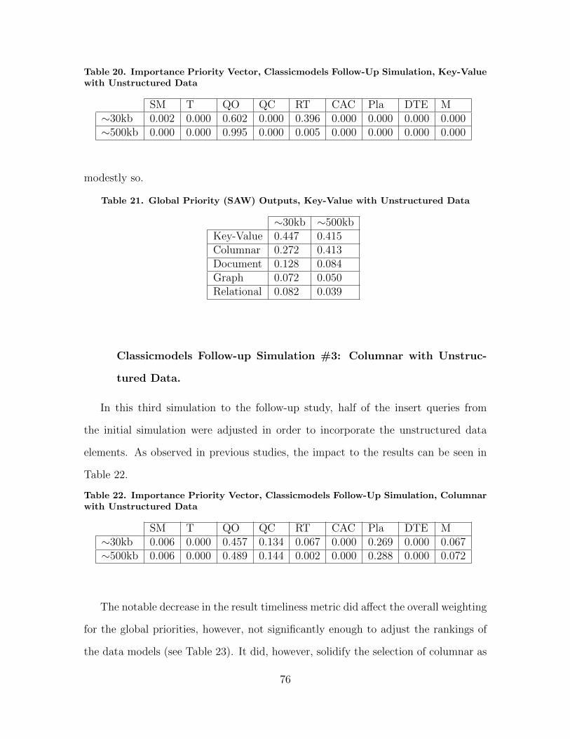
Table 20. Importance Priority Vector, Classicmodels Follow-Up Simulation, Key-Valuewith Unstructured Data


modestly so.

Table 21. Global Priority (SAW) Outputs, Key-Value with Unstructured Data

∼30kb ∼500kbKey-Value 0.447 0.415Columnar 0.272 0.413Document 0.128 0.084Graph 0.072 0.050Relational 0.082 0.039

Classicmodels Follow-up Simulation #3: Columnar with Unstruc-

tured Data.

In this third simulation to the follow-up study, half of the insert queries from

the initial simulation were adjusted in order to incorporate the unstructured data

elements. As observed in previous studies, the impact to the results can be seen in

Table 22.

Table 22. Importance Priority Vector, Classicmodels Follow-Up Simulation, Columnarwith Unstructured Data


The notable decrease in the result timeliness metric did affect the overall weighting

for the global priorities, however, not significantly enough to adjust the rankings of

the data models (see Table 23). It did, however, solidify the selection of columnar as

76

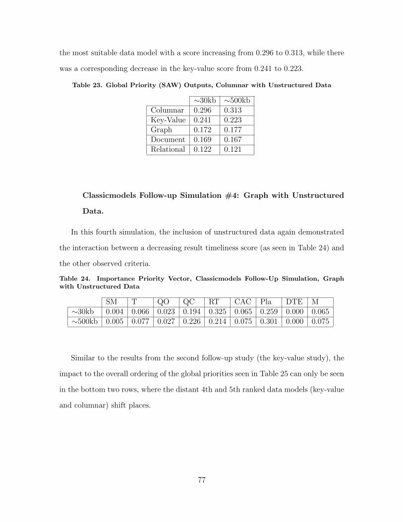
the most suitable data model with a score increasing from 0.296 to 0.313, while there

was a corresponding decrease in the key-value score from 0.241 to 0.223.

Table 23. Global Priority (SAW) Outputs, Columnar with Unstructured Data

∼30kb ∼500kbColumnar 0.296 0.313Key-Value 0.241 0.223Graph 0.172 0.177Document 0.169 0.167Relational 0.122 0.121

Classicmodels Follow-up Simulation #4: Graph with Unstructured

Data.

In this fourth simulation, the inclusion of unstructured data again demonstrated

the interaction between a decreasing result timeliness score (as seen in Table 24) and

the other observed criteria.

Table 24. Importance Priority Vector, Classicmodels Follow-Up Simulation, Graphwith Unstructured Data


Similar to the results from the second follow-up study (the key-value study), the

impact to the overall ordering of the global priorities seen in Table 25 can only be seen

in the bottom two rows, where the distant 4th and 5th ranked data models (key-value

and columnar) shift places.

77

Table 25. Global Priority (SAW) Outputs, Graph with Unstructured Data

∼30kb ∼500kbGraph 0.239 0.261Relational 0.217 0.228Document 0.209 0.211Columnar 0.141 0.155Key-Value 0.195 0.146

Classicmodels Follow-up Simulation #5: Document with Unstruc-

tured Data.

In the final follow-up simulation, the strategy was to emulate the type of behav-

ior that might be seen if a relational database was used similar to how a document

data model would be used, so this test involved the addition of a large number of

tables, as well as adding many new elements within existing tables. This resulted

in many sparsely populated tables similar to how documents might have many dif-

ferent elements from one aggregate to another. The result of this simulation was

a high number of queries classified under the plasticity criterion and the structural

malleability criterion (shown in Table 26).

Table 26. Importance Priority Vector, Classicmodels Follow-Up Simulation, Documentwith Unstructured Data


A high plasticity score will support the document, column, and graph data mod-

els, while a high structural malleability score primarily supports the key-value and

document data models. As both of these criteria support the document data model,

it was given the highest ranking. Table 27 shows the slight impact to the global

priority outputs as a result of adjusting the image size, which led to a decrease in

78

result timeliness between the two runs.

Table 27. Global Priority (SAW) Outputs, Document with Unstructured Data

∼30kb ∼500kbDocument 0.299 0.299Graph 0.278 0.279Columnar 0.246 0.246Key-Value 0.095 0.092Relational 0.081 0.084

3.9 Conclusion

The results of the pilot studies demonstrated that each of the sets of queries which

were built to showcase typical usage patterns for a given data model were ultimately

selected by ECAT as the highest-ranked (i.e., most suitable) data model. This study

provided a level of validation for the viability of the ECAT software to accurately

characterize observed database usage, and for the methodology as a whole.

Thus, the next step in this research involved applying this methodology to the

three open-source use cases introduced in Section 3.4. That is, the environments for

each use case were constructed and software agents employed to generate the usage

data to be observed. Following the collection of this data, the ECAT tool counted the

number of observations for each of the nine criteria. These results were then fed into

the SAW model, and the rank-ordered results for each of the observed use cases was

determined. The results of this experimental setup and the simulations are discussed

next in Chapter 4.

79

IV. Findings

4.1 Introduction

This chapter discusses the findings of this research. First, the results of the sim-

ulation studies that were described in Chapter 3 are presented. Then, a discussion

of the findings from the simulation results is offered. Finally, the research questions

and hypotheses that were previously introduced are now addressed.

4.2 Simulation Results

For each of the three use cases (i.e., phpBB, Elgg, and PowerDNS) the parameters

for each simulation described in Section 3.4 were adjusted in order understand the

effects of changing the system’s behavior on the simulation outputs. The general

configurations, descriptions of the observed queries, and the observed results are

discussed in this section.

In each of these simulations, as the queries were being collected the data was

periodically analyzed by ECAT until the output results began to stabilize. In the

interest of time, simulations were manually terminated once the SAW output results

converged and remained consistent to three decimal places across subsequent mea-

surements.

phpBB.

For the phpBB use case, four discrete simulations were run. During each simula-

tion, the agents running on each of the client systems interacted with the phpBB web

application according to the general profile described in Section 3.4, performing the

type of actions that would be typical of a system user (e.g., navigating the website,

80

creating and reading content, etc.). Each simulation was designed to adjust the gen-

eral behavior of the agents from one simulation to another to determine the impact

that the change in behavior would have on the ECAT outputs, however, the general

core of the code used to execute these agents can be found in Appendix C.

phpBB Simulation #1.

In this first simulation, each agent was programmed to pseudo-randomly choose

between 32 and 42 actions to accomplish (average = 36.96, σ = 3.76), resulting

in the following average number of actions performed each session: reading threads

(average = 27.30, σ = 3.02), browsing sub-forums (average = 6.12, σ = 0.88),

creating new threads (average = 0.78, σ = 0.42), and creating new comments

(average = 0.77, σ = 0.42). Finally, logging in and out accounted for two actions in

each simulation run.

A total of 2,369 sessions were launched generating a total of 2,377,164 observed

queries. Of those, 1,751,014 queries were retained for analysis and 626,150 queries

were omitted by the ECAT tool (overhead commands such as “administrator com-

mand”, “version()”, “set session sql mode”, etc. do not provide useful information to

the analysis and therefore are discarded). Six of the nine criteria were observed dur-

ing this simulation run and the normalized counts of each criteria are given in Table

28. Due to the extremely small number of occurrences of queries that triggered the

cross-aggregate consistency criterion (N = 6), this value was not significant enough

to be reported at three decimal places.

Table 28. Importance Priority Vector, phpBB Simulation 1


Of the remaining five criteria that were identified, query omniscience was the

81

highest value (0.310), followed by result timeliness (0.295). These two factors both

heavily support the key-value data model (see Figure 8) and, as a result, the SAW

calculation selected this data model as the most suitable for the given use case (see

Table 29).

Table 29. Global Priority (SAW) Outputs, phpBB Simulation 1

Key-Value 0.289Relational 0.196Columnar 0.182Document 0.170Graph 0.165

The variability and 95% confidence intervals for the highest ranked data model

(i.e., key-value) are shown in Figure 16. The x-axis in both plots indicate repeating

iterations within the simulation (see Figure 10, so each dot represents one epoch of

agent executions, and then the aggregate of observed data (i.e., all observed SQL

statements that have been collected to date). The variance plot shows the variability

in the results, on a sliding scale for the 4 most recent epochs. As seen here, the

variance drops off quickly after the first few iterations and falls to 2.95 × 10−9, which

is well below the established threshold of 1 × 10−5. Regarding the 95% confidence

interval, it represents probability that the final result falls within the shaded region,

based on the aggregated measurements for each epoch. Regarding the 95% confidence

interval plot, the blue dots represent the normalized score for this data model as

reported by the SAW decision model at each iteration of the simulation. The final

results for the 95% confidence interval fell within the range of [.286, .291], which is

also well below the desired range of .01. In this and following sections, the data for

the remaining four data models are not shown for the sake of space, however they all

follow similar trends to the key-value results and fall below the established thresholds.

82

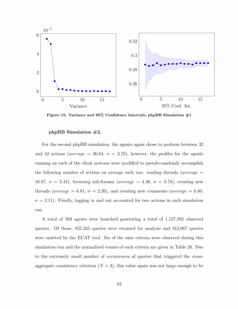
0 5 10 15

0

2

4

6·10−5

Variance

0 5 10 15

0.26

0.28

0.3

0.32

95% Conf. Int.

Figure 15. Variance and 95% Confidence Intervals, phpBB Simulation #1


For the second phpBB simulation, the agents again chose to perform between 32

and 42 actions (average = 36.84, σ = 3.78), however, the profiles for the agents

running on each of the client systems were modified to pseudo-randomly accomplish

the following number of actions on average each run: reading threads (average =

16.87, σ = 3.44), browsing sub-forums (average = 4.36, σ = 0.78), creating new

threads (average = 6.81, σ = 2.26), and creating new comments (average = 6.80,

σ = 2.11). Finally, logging in and out accounted for two actions in each simulation

run.

A total of 569 agents were launched generating a total of 1,137,392 observed

queries. Of those, 825,325 queries were retained for analysis and 312,067 queries

were omitted by the ECAT tool. Six of the nine criteria were observed during this

simulation run and the normalized counts of each criteria are given in Table 28. Due

to the extremely small number of occurrences of queries that triggered the cross-

aggregate consistency criterion (N = 3), this value again was not large enough to be

83

reported at three decimal places.



As seen in Table 30, the change in ratios of the observed query was negligible from

the first phpBB simulation. As a result, the SAW calculation again selected key-value

as the most suitable data model for this use case (see Table 31).




(i.e., key-value) are shown in Figure 16. As before, the variance drops off quickly

after the first few iterations and progresses to 1.18 × 10−7, well below the established

threshold of 1 × 10−5. Regarding the 95% confidence interval, the final results fell

within the range of [.292, .295], still below the established threshold of .01.

84

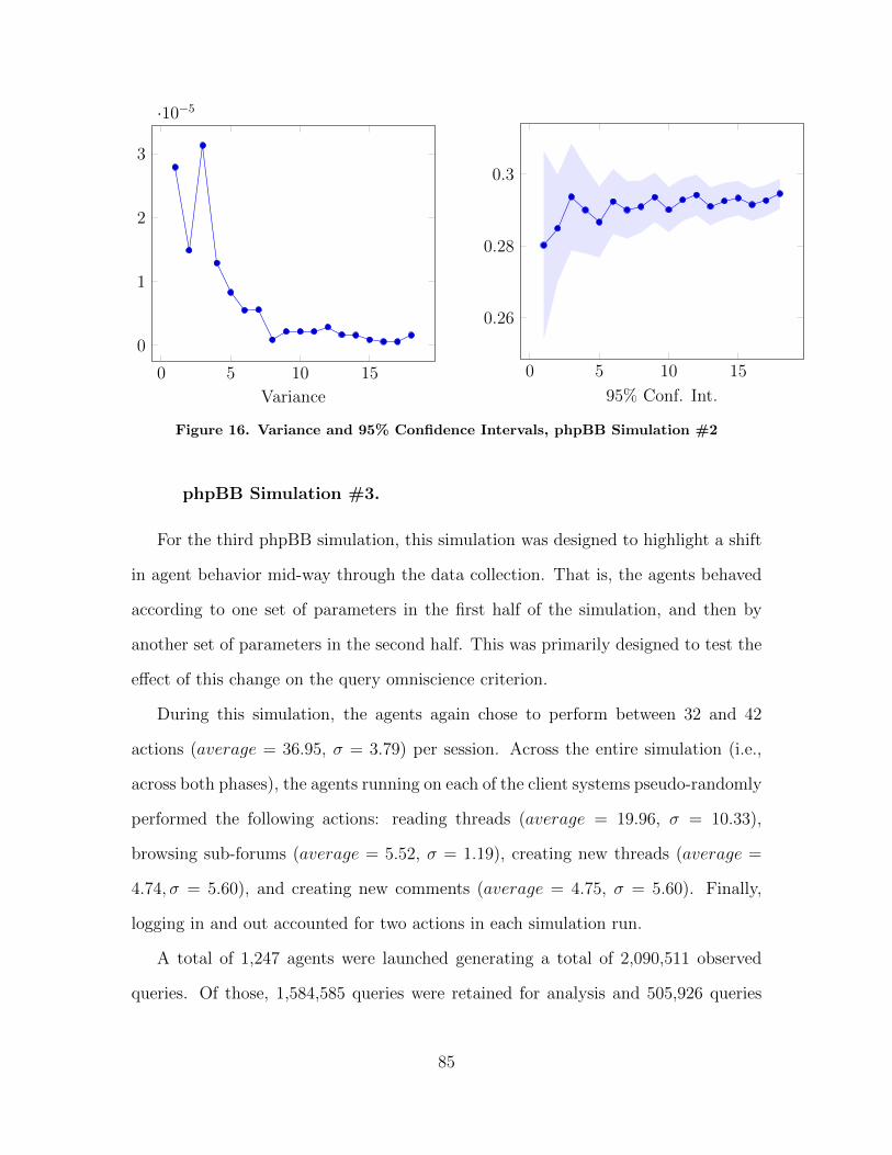
0 5 10 15

0

1

2

3

·10−5

Variance

0 5 10 15

0.26

0.28

0.3

95% Conf. Int.



For the third phpBB simulation, this simulation was designed to highlight a shift

in agent behavior mid-way through the data collection. That is, the agents behaved

according to one set of parameters in the first half of the simulation, and then by

another set of parameters in the second half. This was primarily designed to test the

effect of this change on the query omniscience criterion.

During this simulation, the agents again chose to perform between 32 and 42

actions (average = 36.95, σ = 3.79) per session. Across the entire simulation (i.e.,

across both phases), the agents running on each of the client systems pseudo-randomly

performed the following actions: reading threads (average = 19.96, σ = 10.33),

browsing sub-forums (average = 5.52, σ = 1.19), creating new threads (average =

4.74, σ = 5.60), and creating new comments (average = 4.75, σ = 5.60). Finally,

logging in and out accounted for two actions in each simulation run.

A total of 1,247 agents were launched generating a total of 2,090,511 observed

queries. Of those, 1,584,585 queries were retained for analysis and 505,926 queries

85

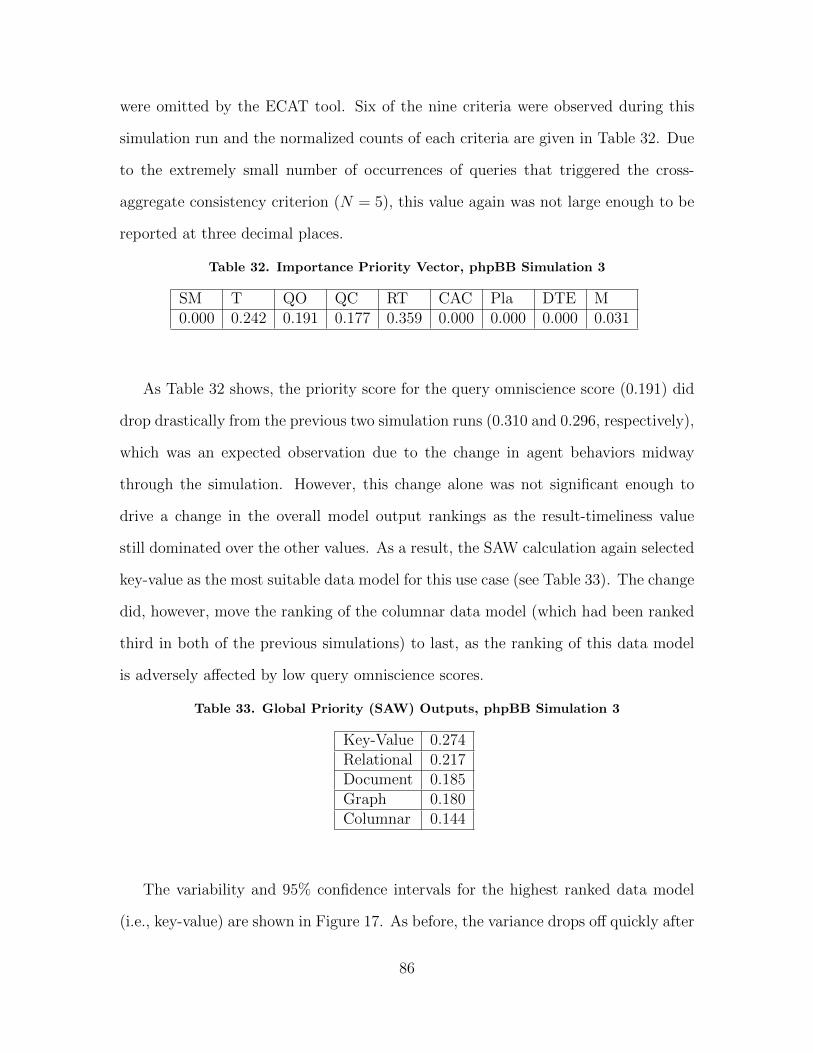
were omitted by the ECAT tool. Six of the nine criteria were observed during this

simulation run and the normalized counts of each criteria are given in Table 32. Due

to the extremely small number of occurrences of queries that triggered the cross-

aggregate consistency criterion (N = 5), this value again was not large enough to be

reported at three decimal places.



As Table 32 shows, the priority score for the query omniscience score (0.191) did

drop drastically from the previous two simulation runs (0.310 and 0.296, respectively),

which was an expected observation due to the change in agent behaviors midway

through the simulation. However, this change alone was not significant enough to

drive a change in the overall model output rankings as the result-timeliness value

still dominated over the other values. As a result, the SAW calculation again selected

key-value as the most suitable data model for this use case (see Table 33). The change

did, however, move the ranking of the columnar data model (which had been ranked

third in both of the previous simulations) to last, as the ranking of this data model

is adversely affected by low query omniscience scores.


Key-Value 0.274Relational 0.217Document 0.185Graph 0.180Columnar 0.144


(i.e., key-value) are shown in Figure 17. As before, the variance drops off quickly after

86

the first few iterations, however it spikes in the middle. This is expected, since the

agent’s behavior during the simulation also dramatically shifts at the mid-point. The

variance again drops off quickly after the behavior shift occurs as the agents continue

to follow their new pattern, resulting in a final variance of 4.39 × 10−7. Regarding

the 95% confidence interval, the final results fell within the range of [.271, .277], also

below the established threshold of .01.

0 5 10 15 20 25 30

0

0.5

1

1.5

2

2.5·10−5

Variance

0 5 10 15 20 25 300.26

0.27

0.28

0.29

0.3

0.31

95% Conf. Int.



A fourth and final phpBB simulation was designed to test the effect of sending

large amounts of semi-structured text through the phpBB web application to the

database and observe the impact of this change. Although the web application was

designed to support field entries of up to 16MB, in practice the web application would

frequently time out for results of only a few (i.e., 1-4) megabytes. Thus, the results

of this run were not included in this research due to low-confidence in the reliability

of the data.

87

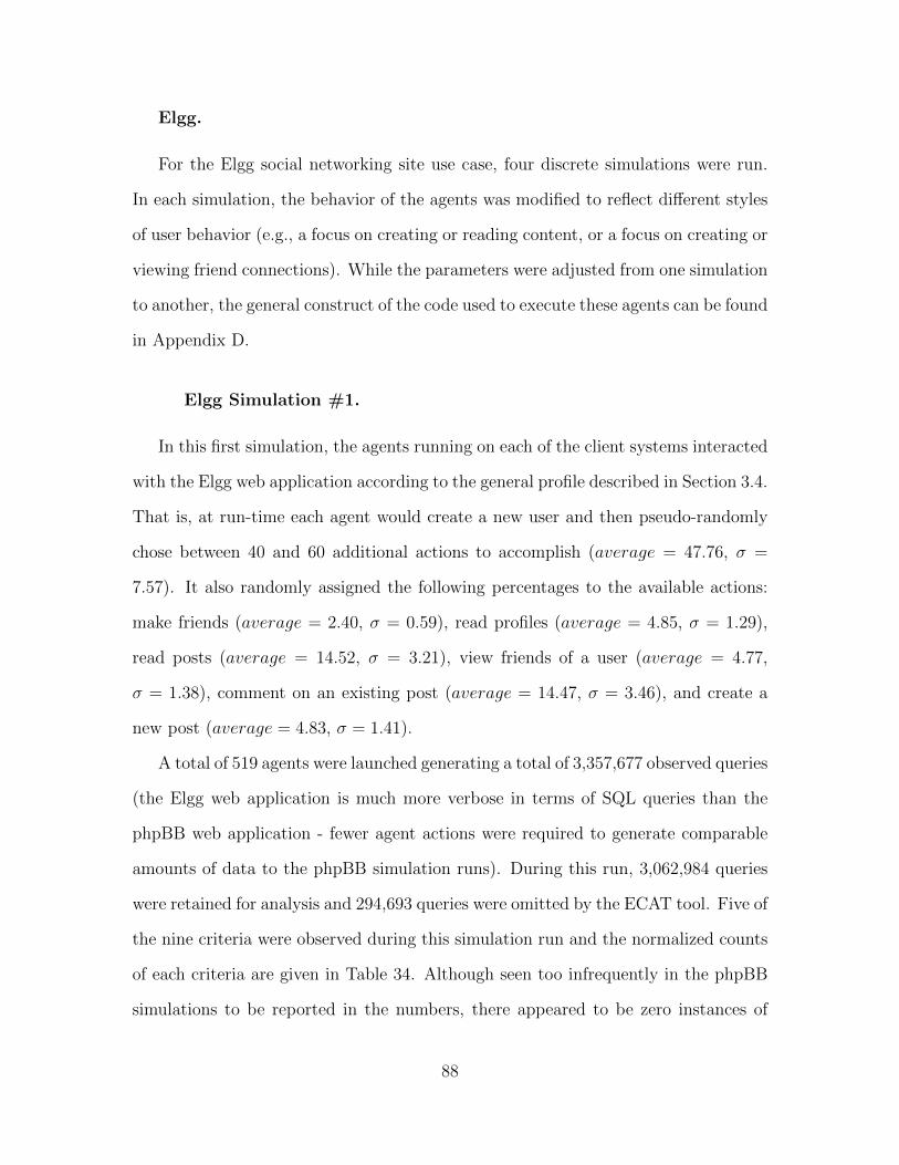
Elgg.

For the Elgg social networking site use case, four discrete simulations were run.

In each simulation, the behavior of the agents was modified to reflect different styles

of user behavior (e.g., a focus on creating or reading content, or a focus on creating or

viewing friend connections). While the parameters were adjusted from one simulation

to another, the general construct of the code used to execute these agents can be found

in Appendix D.

Elgg Simulation #1.

In this first simulation, the agents running on each of the client systems interacted

with the Elgg web application according to the general profile described in Section 3.4.

That is, at run-time each agent would create a new user and then pseudo-randomly

chose between 40 and 60 additional actions to accomplish (average = 47.76, σ =

7.57). It also randomly assigned the following percentages to the available actions:

make friends (average = 2.40, σ = 0.59), read profiles (average = 4.85, σ = 1.29),

read posts (average = 14.52, σ = 3.21), view friends of a user (average = 4.77,

σ = 1.38), comment on an existing post (average = 14.47, σ = 3.46), and create a

new post (average = 4.83, σ = 1.41).

A total of 519 agents were launched generating a total of 3,357,677 observed queries

(the Elgg web application is much more verbose in terms of SQL queries than the

phpBB web application - fewer agent actions were required to generate comparable

amounts of data to the phpBB simulation runs). During this run, 3,062,984 queries

were retained for analysis and 294,693 queries were omitted by the ECAT tool. Five of

the nine criteria were observed during this simulation run and the normalized counts

of each criteria are given in Table 34. Although seen too infrequently in the phpBB

simulations to be reported in the numbers, there appeared to be zero instances of

88

cross-aggregate consistency criterion in the Elgg use case which is why that criterion

is not observed here.

Table 34. Importance Priority Vector, Elgg Simulation 1


Of the five criteria that were identified, query omniscience was the highest value

(0.318), followed by result timeliness (0.290). These two factors were the dominant

factors in the first two phpBB simulations. Again, as they both heavily support the

key-value data model (see Figure 8) the SAW calculation selected this data model as

the most suitable for the given use case (see Table 35).

Table 35. Global Priority (SAW) Outputs, Elgg Simulation 1



(i.e., key-value) are shown in Figure 18. The variance remains low throughout the

entire simulation with a final measurement of 1.25 × 10−10. Regarding the 95% con-

fidence interval, the final results fell within the range of [.292, .293], also below the

established threshold of .01.

89

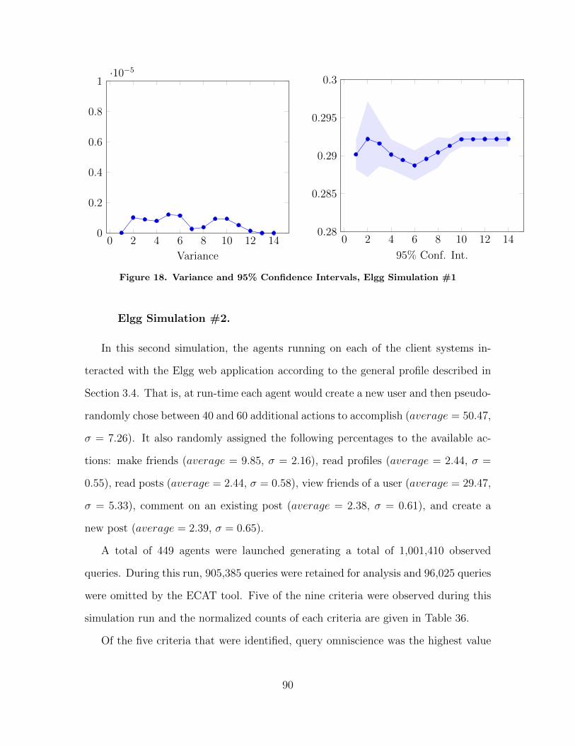
0 2 4 6 8 10 12 140

0.2

0.4

0.6

0.8

1·10−5

Variance

0 2 4 6 8 10 12 140.28

0.285

0.29

0.295

0.3

95% Conf. Int.

Figure 18. Variance and 95% Confidence Intervals, Elgg Simulation #1

Elgg Simulation #2.

In this second simulation, the agents running on each of the client systems in-

teracted with the Elgg web application according to the general profile described in

Section 3.4. That is, at run-time each agent would create a new user and then pseudo-

randomly chose between 40 and 60 additional actions to accomplish (average = 50.47,

σ = 7.26). It also randomly assigned the following percentages to the available ac-

tions: make friends (average = 9.85, σ = 2.16), read profiles (average = 2.44, σ =

0.55), read posts (average = 2.44, σ = 0.58), view friends of a user (average = 29.47,




queries. During this run, 905,385 queries were retained for analysis and 96,025 queries

were omitted by the ECAT tool. Five of the nine criteria were observed during this

simulation run and the normalized counts of each criteria are given in Table 36.


90



(0.319), followed closely by result timeliness (0.304). Again, as they both heavily

support the key-value data model (see Figure 8) the SAW calculation selected this

data model as the most suitable for the given use case (see Table 37).


Key-Value 0.297Relational 0.200Columnar 0.180Graph 0.163Document 0.161


(i.e., key-value) are shown in Figure 19. The variance remains low throughout the

entire simulation with a final measurement of 4.25 × 10−8. Regarding the 95% con-

fidence interval, the final results fell within the range of [.296, .298], also below the

established threshold of .01.

91

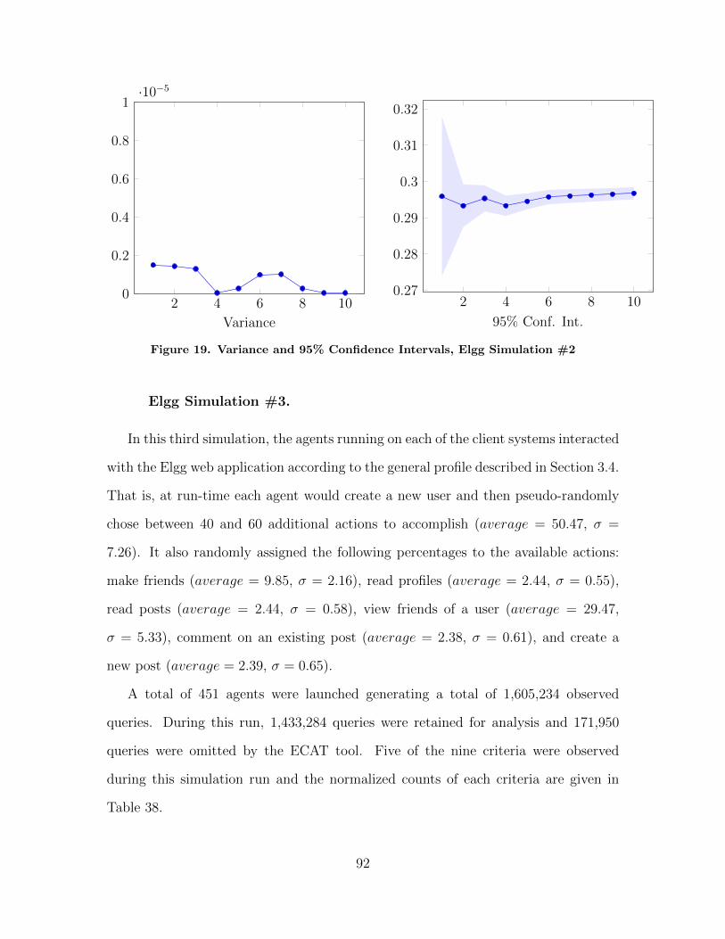
2 4 6 8 100

0.2

0.4

0.6

0.8

1·10−5

Variance

2 4 6 8 100.27

0.28

0.29

0.3

0.31

0.32

95% Conf. Int.


Elgg Simulation #3.

In this third simulation, the agents running on each of the client systems interacted

with the Elgg web application according to the general profile described in Section 3.4.

That is, at run-time each agent would create a new user and then pseudo-randomly

chose between 40 and 60 additional actions to accomplish (average = 50.47, σ =

7.26). It also randomly assigned the following percentages to the available actions:

make friends (average = 9.85, σ = 2.16), read profiles (average = 2.44, σ = 0.55),

read posts (average = 2.44, σ = 0.58), view friends of a user (average = 29.47,




queries. During this run, 1,433,284 queries were retained for analysis and 171,950

queries were omitted by the ECAT tool. Five of the nine criteria were observed

during this simulation run and the normalized counts of each criteria are given in

Table 38.

92




(0.320), followed again by result timeliness (0.300). As before, they both heavily

support the key-value data model (see Figure 8), thus the SAW calculation selected

this data model as the most suitable for the given use case (see Table 39).


Key-Value 0.299Relational 0.198Columnar 0.182Graph 0.161Document 0.161


(i.e., key-value) are shown in Figure 20. The variance falls quickly after the first few

iterations and then remains low throughout the remainder of the simulation with a

final measurement of 2.67 × 10−7. Regarding the 95% confidence interval, the final

results fell within the range of [.297, .301], also below the established threshold of .01.

93

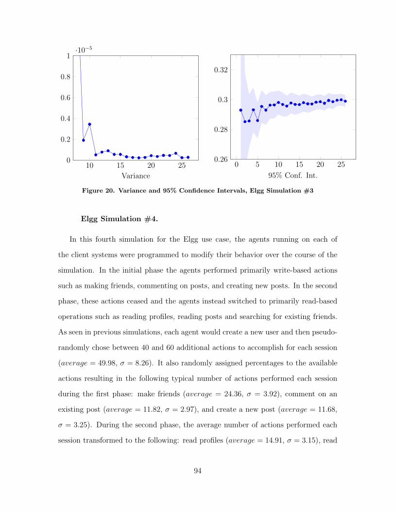
10 15 20 250

0.2

0.4

0.6

0.8

1·10−5

Variance

0 5 10 15 20 250.26

0.28

0.3

0.32

95% Conf. Int.


Elgg Simulation #4.

In this fourth simulation for the Elgg use case, the agents running on each of

the client systems were programmed to modify their behavior over the course of the

simulation. In the initial phase the agents performed primarily write-based actions

such as making friends, commenting on posts, and creating new posts. In the second

phase, these actions ceased and the agents instead switched to primarily read-based

operations such as reading profiles, reading posts and searching for existing friends.

As seen in previous simulations, each agent would create a new user and then pseudo-

randomly chose between 40 and 60 additional actions to accomplish for each session

(average = 49.98, σ = 8.26). It also randomly assigned percentages to the available

actions resulting in the following typical number of actions performed each session

during the first phase: make friends (average = 24.36, σ = 3.92), comment on an

existing post (average = 11.82, σ = 2.97), and create a new post (average = 11.68,

σ = 3.25). During the second phase, the average number of actions performed each

session transformed to the following: read profiles (average = 14.91, σ = 3.15), read

94

posts (average = 14.74, σ = 3.15), and view friends of a user (average = 19.44,

σ = 3.87).

A total of 200 agents were launched generating a total of 1,001,410 observed queries

(the Elgg web application is much more verbose in terms of SQL queries than the

phpBB web application - fewer agent actions were required to generate comparable

amounts of data to the phpBB simulation runs). During this run, 905,385 queries

were retained for analysis and 96,025 queries were omitted by the ECAT tool. Five of

the nine criteria were observed during this simulation run and the normalized counts

of each criteria are given in Table 40.



Of the five criteria that were identified, result timeliness was the highest value

(0.320), followed by query omniscience (0.271). The query omniscience score observed

here was lower than in the previous Elgg simulations, which was an anticipated out-

come for this simulation based on the dramatic shift in user behavior between the

first part of the simulation and the second. As before, these criteria both heavily

support the key-value data model (see Figure 8) the SAW calculation selected this

data model as the most suitable for the given use case (see Table 41).


Key-Value 0.286Relational 0.212Graph 0.171Document 0.167Columnar 0.164


95

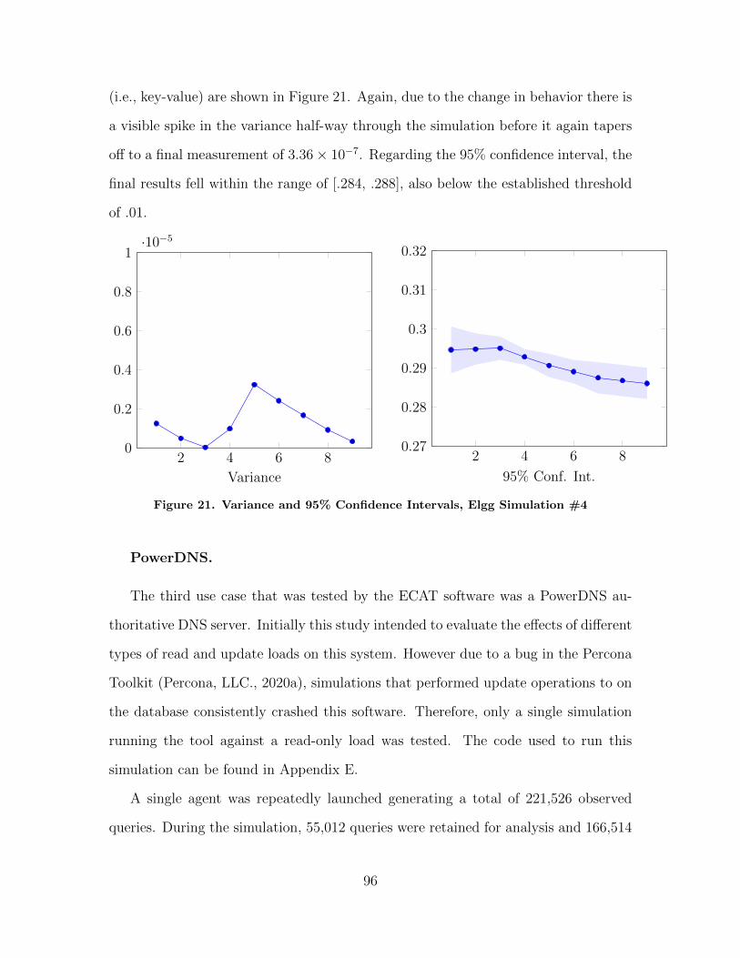
(i.e., key-value) are shown in Figure 21. Again, due to the change in behavior there is

a visible spike in the variance half-way through the simulation before it again tapers

off to a final measurement of 3.36 × 10−7. Regarding the 95% confidence interval, the

final results fell within the range of [.284, .288], also below the established threshold

of .01.

2 4 6 80

0.2

0.4

0.6

0.8

1·10−5

Variance

2 4 6 80.27

0.28

0.29

0.3

0.31

0.32

95% Conf. Int.


PowerDNS.

The third use case that was tested by the ECAT software was a PowerDNS au-

thoritative DNS server. Initially this study intended to evaluate the effects of different

types of read and update loads on this system. However due to a bug in the Percona

Toolkit (Percona, LLC., 2020a), simulations that performed update operations to on

the database consistently crashed this software. Therefore, only a single simulation

running the tool against a read-only load was tested. The code used to run this

simulation can be found in Appendix E.

A single agent was repeatedly launched generating a total of 221,526 observed

queries. During the simulation, 55,012 queries were retained for analysis and 166,514

96

queries were omitted by the ECAT tool. Owing to the low diversity in the types of

observed queries (only five distinct types of queries were observed), this simulation

only triggered four of the nine criteria. The normalized counts of each criteria are

given in Table 42.

Table 42. Importance Priority Vector, PowerDNS Simulation 1


Of the four criteria that were identified, result timeliness was the highest value

(0.412), followed closely by query omniscience (0.411). These two factors had also

been the dominant factors in the first two phpBB simulations, but the relatively

lower counts on all other metrics only served to increase the selection of the key-

value data model (see Figure 8) even more. The key-value rating of (0.381) was the

highest seen in any of the simulations (see Table 43). Given that the DNS use case

was selected because of its suitability for the key-value data model (a simple system

based on a non-complex key lookup with an emphasis on speed), this outcome was

not surprising. What was noteworthy was that the high query omniscience score for

this use case resulted in columnar being selected as the second most suitable model

(where it had ranked no higher than third in any of the previous simulation runs).

Table 43. Global Priority (SAW) Outputs, PowerDNS Simulation 1

Key-Value 0.381Columnar 0.210Document 0.156Relational 0.137Graph 0.116


(i.e., key-value) are shown in Figure 22. Given the simplicity of this simulation and

97

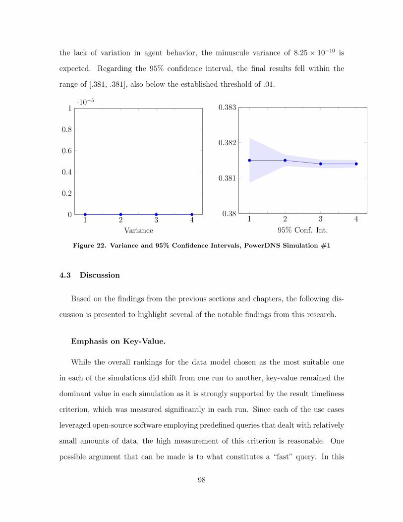
the lack of variation in agent behavior, the minuscule variance of 8.25 × 10−10 is

expected. Regarding the 95% confidence interval, the final results fell within the

range of [.381, .381], also below the established threshold of .01.

1 2 3 40

0.2

0.4

0.6

0.8

1·10−5

Variance

1 2 3 40.38

0.381

0.382

0.383

95% Conf. Int.

Figure 22. Variance and 95% Confidence Intervals, PowerDNS Simulation #1

4.3 Discussion

Based on the findings from the previous sections and chapters, the following dis-

cussion is presented to highlight several of the notable findings from this research.

Emphasis on Key-Value.

While the overall rankings for the data model chosen as the most suitable one

in each of the simulations did shift from one run to another, key-value remained the

dominant value in each simulation as it is strongly supported by the result timeliness

criterion, which was measured significantly in each run. Since each of the use cases

leveraged open-source software employing predefined queries that dealt with relatively

small amounts of data, the high measurement of this criterion is reasonable. One

possible argument that can be made is to what constitutes a “fast” query. In this

98

research, one millisecond was used as the threshold because many (but not all) of the

observed queries in this research operated under or near that threshold. However, as

demonstrated in the follow-up pilot study in Chapter 2, once the average data sizes

began to increase to ∼500 kb, this metric began to drop significantly so there is a

significant trade-off between the average query size and the speed of the results.

Sensitivity of Query Omniscience Measurements.

The query omniscience criterion seeks to measure the “degree to which the com-

plete set of possible queries is known by the user before (the) system is implemented”

(Engle, 2018). Since a stated goal of this research was to attempt to infer the Engle

criteria without the benefit of interviewing system users, a proxy measurement was

proposed in which the types of queries observed by the system would be compared

over time. If the types of queries seen at the beginning of the analysis were different

than those seen at the end, an argument can be made that the usage of the system

shifted during the course of its execution and the complete set of possible queries may

not have been known at the onset.

However, a pitfall of this approach is that it assumes data is being collected over

a long period of time (at least long enough to capture any shifts in behavior that may

have occurred). If the methodology was only applied to a brief snapshot in time (e.g.,

a hour or less), then it is foreseeable that specific events could skew this measurement.

For example, if during the hour of observation a large amount of data is written into

the database in the beginning and then read back out or updated heavily in the latter

part of the hour, then ECAT would likely detect this as a significant shift in the type

of usage and assign it a low query omniscience score. On the other hand, if this was

actually a common occurrence (e.g., for some type of daily report) then the results

of this repeated event throughout the course of a week would be smoothed out and

99

the query omniscience score would be reported at a much higher level.

System Overhead.

An unanticipated aspect of this methodology’s approach is the amount of system

overhead in terms of storage and processing requirements that were needed to perform

the analysis. On the data storage side, packet captures were commonly observed to

reach 3-4 times the size of the original data being transmitted due to the verbosity

of these applications. For example, when 32 megabytes of data was transmitted to

and from the database, the resulting packet capture was expected to be close to 64

megabytes in size, plus a reasonable amount for overhead. In reality, the packet

capture during that simulation was observed to be over 250 megabytes. That said, in

order to mitigate any impact from excessive storage requirements it would be possible

to alter the ECAT software to utilize a log rotation-style packet capture strategy, and

then continuously process the data as it arrives to extract and retain only the salient

features required for the analysis. This would allow the large packet captures to then

be discarded reducing the overall storage requirements.

Similarly, the processing necessary to compute the Engle criteria required several

passes over the data (in order to extract the queries, build and track changes to the

schema, and assess each of the 9 measured criteria). While some aspects of the ECAT

software could have been parallelized in order to improve performance, most of the I/O

heavy operations (including all results from the Percona Toolkit) were single-threaded

which bottle-necked the overall throughput. In practice, the simulation was able to

generate data faster than it could be processed by ECAT. As a result, depending on

the volume and velocity of observed traffic the system performing the ECAT analysis

may require significant computational resources to keep up. For reference, the second

Elgg simulation resulted in a packet capture that was 5.5 gigabytes in size. Ten agents

100

running at full speed were able to generate this file in only 2 hours and 11 minutes,

while the complete processing of this file required three hours and 45 minutes on a

virtual machine equipped with 8 virtual CPUs (vCPU) from a Intel Xeon CPU E5-

2687W V2 operating at 3.40 GHz (again, due to the single-threaded nature of the

software, only a single vCPU was in use by ECAT for processing of the data at any

given time).

Viability of Results.

Despite these shortcomings, the initial pilot studies discussed in Chapter 3 and

the three use case simulations presented here in Chapter 4 have demonstrated that

there are measurable characteristics of the Engle criteria which can be captured and

assessed solely through observation of a user’s or application’s interactions with a

relational database. Furthermore, these measurements can be used to produce a

rank-ordered assessment of the suitability of the relational and NoSQL data models

for the observed usage. This assessment provides the user not only with insights

about how their system is being used, but may also ultimately point them towards

considering an alternative underlying data model which may be more suitable for

their system.

4.4 Conclusions of Research

The first research question asked “Which observable criteria exist for assessing

the usage patterns of a non-distributed relational database in an automated fash-

ion?” This question was intended to identify which kinds of criteria were available

in order to help inform the selection of a suitable underlying data model, and the

research previously conducted by Engle served as an excellent foundation to build

upon. That research (and its associated methodology for identifying suitable data

101

models based on the intended or perceived usage of a database system) introduced a

comprehensive list of 12 criteria that evaluated many important aspects of a system’s

usage. Through critical, subjective assessments by system subject matter experts,

those 12 criteria would be compared and prioritized to help a decision-maker deter-

mine what underlying data model was the most suitable based on their individual

preferences.

Although all 12 of the criteria provide useful inputs for evaluating a given solu-

tion, not all aspects were found to be observable in practice (from the perspective of

observing database usage in an automated fashion). The methodology presented in

this research was developed in order to determine which of the existing criteria could

be measured through an automated assessment of database usage, and additionally,

to what extent. The development of the ECAT software, along with the pilot studies

and simulations performed during this research, demonstrated that a subset of the

original 12 criteria could be evaluated against observations of an existing relational

database system. Due to limitations inherent in this approach, measurements for one

of the criterion was deemed to be not possible (i.e., pre-processing), while measure-

ments for other two other criteria were considered to be theoretically achievable, yet

finding a means of identifying them remained elusive during this research (i.e, large

and small aggregate transactions). The results of the pilot studies and simulations

ultimately produced a number of findings and insights about how the observation and

assessment of those criteria could help a user understand which criteria were actually

being observed in their systems.

The second research question builds upon the first one when it asks: “Using an

automated methodology, can non-distributed relational database usage patterns be

mapped to more suitable data models using the observable criteria?” The outputs

from both the pilot studies and the simulations demonstrated that this methodology

102

is able to employ the observable criteria as inputs to a decision model which provides

information to a user regarding the suitability of the NoSQL data models based solely

on those observations of interactions with an existing relational database. However,

due to some of the limitations of this approach (e.g., not all criteria are able to

be measured and thus given equal consideration), it cannot provably say that an

alternative NoSQL solution would be the “most” suitable for the given usage based

on the limited set of information available to such a system. Rather, it would be

more defensible to claim that this methodology does provide the user with insights

about how an existing database system is being used, and based on the observations

of system usage it is able to provide a suggested mapping to suitability NoSQL data

models, justified by the observable characteristics that were measured.

Research Hypotheses.

As stated in Section 3.2, this research explored three hypotheses, repeated here:

1. One or more elements of the Engle criteria can be mapped to observable char-

acteristics of relational database systems.






Through the development of the ECAT software and its application to the pilot

studies and experimental simulations, the first research hypothesis can be definitively

answered to be true. Although only a subset of the original 12 Engle criteria could be

evaluated, the ECAT software did demonstrate that the remaining nine criteria could

103

be assessed through observable characteristics of an existing relational database sys-

tem. Furthermore, the pilot studies and experimental simulations also demonstrated

that adjustments to the “behaviors” of agents using those systems did produce mea-

surable changes in the outputs of the ECAT software in order to profile the usage

of those systems. Thus, the second research hypothesis was also supported. Finally,

the profiled usage of a database system (based on a subset of the original 12 Engle

criteria) was shown to be useful as an input into a Simple Additive Weighting MCDM

model that is able to characterize the suitability of NoSQL data models based on the

observed usage. Thus, the final research hypothesis was also shown to be true.

104

V. Conclusions, Significance of Research, & FutureConsiderations

5.1 Chapter Overview

Chapter 2 introduced key concepts and trends relating to database storage mod-

els beginning with the relational data model in the 1970’s through today’s mod-

ern NoSQL data models. Also presented was a discussion of typical use cases for

NoSQL databases, previous work on characterizing database usage patterns on non-

distributed systems, and a treatment on the multi-criteria decision-making processes

underlying this research. This provided a theoretical foundation for the discussion

that followed.

Next, Chapter 3 continued onward from the theoretical foundation laid in Chap-

ter 2 with the introduction of a methodology to identify alternative suitable NoSQL

data models solely through the observation of user/application interactions with a

relational database system. This novel approach to characterizing the usage of an

existing database system through the assessment of observed usage data was demon-

strated through two pilot studies which illustrated how the Engle Criteria Analysis

Tool (ECAT) could be employed to implement this methodology. Additionally, three

distinct use case simulations (phpBB, Elgg, and PowerDNS) were proposed.

Then in Chapter 4, a description of the execution of the experimental setup for

the three simulations described in Chapter 3 was presented, along with the results

from those simulations. The chapter concluded with a discussion of the results and

the research findings and addressed how the research questions and hypotheses were

answered in the course of this research.

Finally, this chapter now highlights the contributions of my research and proposes

recommendations for future research.

105

5.2 Significance of Research

This research was built upon the foundations laid by previous researchers (En-

gle, 2018; Hecht & Jablonski, 2011) who characterized various aspects of database

usage in order to assess the suitability of an underlying data model. However, this

research was novel in several ways. First, this research represents the first attempt to

characterize the usage of an existing database by extracting queries through network

packet sniffing. Although the open-source toolkit used to extract the queries from

packet captures has generally been used by database administrators to troubleshoot

aspects of system performance, there are no indications in the literature to suggest

that anyone has yet attempted to aggregate the results in the manner proposed in

this research in order to profile the usage of a system.

This unprecedented approach at profiling the usage of a system was then incor-

porated into the development of the ECAT software (provided in Appendix A). This

software demonstrated how the captured network packets could be parsed and ana-

lyzed so that the strategies discussed in Section 3.3 for identifying the Engle criteria

could then be applied. This observed usage was used to generate objective mea-

surements of how the system was actually being used in terms of the Engle criteria,

extending the previous work which had employed subjective user inputs as a means

of assessing the most suitable solution. This is not a claim that the methodology pre-

sented here is superior to the existing one; rather, the significance of this approach is

that lends a new, alternative perspective to an existing problem.

Finally, by taking the objective measurements produced by ECAT and incorpo-

rating them with the performance priorities for each of the data models via a Simple

Additive Weighting model, this research demonstrated the ability of this methodology

to produce a suitability ranking of each of the five data models (relational, key-value,

document, columnar, and graph) based solely on observations of a system’s usage.

106

There are several benefits to be realized by the practical applications of this re-

search to real-world systems. First, the Engle criteria metrics that are reported by

ECAT can inform the system owner about various aspects of their system’s usage

at a given period in time, as repeated measurements indicating changes in one or

more of the criteria could help the system owner discover changes in the underlying

usage patterns by their users, prompting them to better understand why users are

changing their behavior. Furthermore, this methodology could be applied during ag-

ile software development to help point application developers towards an appropriate

data model during the early stages of a system’s development. Finally, the output

from the SAW decision model indicating that a more suitable data model for a given

application exists may motivate a system owner to conduct a more in-depth analysis

of the potential advantages and trade-offs of switching to the suggested data model.

5.3 Comments on the Methodology

There were a number of limitations inherent in the approach employed during

this research. One of the biggest shortcomings was a lack of access to real-world

usage data. Although this research demonstrates the ease at which this data can

be accessed, concerns relating to privacy, security, and system performance made it

difficult to find system owners who were willing to share this data. By employing open-

source software in the experimental simulations and designing software-based agents

to interact with these systems similar to how human users would, this limitation was

mitigated to the greatest extent possible.

Another limitation of employing this methodology against well-defined software

like phpBB or Elgg is that each of these apps were optimized to perform their key

functions in particular ways. For instance, when navigating to another page in phpBB

(whether the user had just created a new post or was browsing an existing one), the

107

application will use the same types of SQL queries to populate the footer information

(with information such as who else is currently online) which is generated on each page

reload. Receiving this information may not have been the primary objective of the

user at that time, however, the behavior is still being captured through this process.

Thus, even with significant shifts in the user’s behavior, some queries performed by

the underlying app remain unchanged. Therefore, when considering shifts in usage

patterns this factor results in less pronounced changes in output than might have

been otherwise expected for these types of systems.

Engle’s weighting of the transparency criterion (see Figure 8) strongly disfavors

the Key-Value data model, because as discussed in Chapter 2, the aggregate in this

data model is an opaque value to the database system (and thus it is not possible

to retrieve individual elements within the aggregate). Intuitively, it may stand to

reason then that there would be an inverse relationship between the observation of

this criterion and the ranking of the key-value data model (that is, as the transparency

metric increases, the scoring for the key-value data model should decrease). However,

in practice the opposite was seen to be true. The measurement of the transparency

criterion in this research was based on the observation of “SELECT” queries, which

were almost universally observed executing in the sub-millisecond time frame. As a

result, even in instances where there was a high reported value for the transparency

criterion, the extremely strong weighting of the result timeliness criterion favoring

the key-value data model (0.496) actually overshadowed any advantages to the other

data models for the transparency criterion. As identified during the pilot studies,

this impact tends to be more pronounced when the evaluation primarily consists of

observations of small amounts of structured data. However, for systems dealing with

larger amounts of semi-structured or un-structured data, the result timeliness criterion

would take on a less dramatic role in the model’s scoring. One possible way to address

108

this limitation might also include the inclusion of criterion-specific coefficients which

could dampen or amplify the results for the result timeliness criterion based on the

types of data being observed.

This research sought to understand what characterizations could be made re-

garding the suitability of a NoSQL data model based only on observations of user

interactions with an relational database. Although this provides a second perspec-

tive to the problem, a better solution would likely incorporate inputs from both this

methodology as well as the methodology proposed by Engle in order to provide a

more comprehensive view of the ideal solution.

5.4 Recommendations for Future Research

There are a number of excellent opportunities to extend this research in the future.

First, this research focused on assessing MySQL databases because of the existing

availability of tools to decode and parse the MySQL protocol. However, this method-

ology can theoretically be applied to any SQL-based implementation. Future work in

extending this approach to other SQL-based implementations would help extend the

value of this work to a larger audience of practitioners.

Additionally, future work improving the performance and extending the capabil-

ities of the ECAT software would also serve to increase its value to practitioners.

Rewriting the software to be multi-threaded (where possible) would be one potential

avenue to pursue. Additionally, redesigning it to continuously monitor and assess sys-

tem usage might provide valuable insights into how usage patterns change over time,

which might have implications that extend much further than just the underlying

data model (e.g., system capacity planning, performance issues, etc.).

Furthermore, the value of this methodology could be greatly improved upon

through the development of a method to discriminate between different classes or

109

groups of users. Conceptually, different groups of users might use the same system in

different ways. Observations based on an aggregation of different groups of users may

identify the best solution for the group as a whole. However, considering these groups

separately might reveal that each possess a different “optimal” solution (which then

could potentially be realized through a hybrid database architecture). The addition

of such a capability to this methodology would greatly increase the significance of

this work and the benefit it could provide to users.

Finally, if additional time and resources were made available for this research, the

methodology presented here could be further validated by demonstrating that a data

model ranked ahead of the relational model by ECAT is able to out-perform it using

some objectively quantifiable suitability metric (e.g., overall speed). This could be

accomplished by implementing the database in the alternative NoSQL data model,

adjusting the application code to support the new underlying data model, and then

running the necessary benchmarking tests.

5.5 Summary

The effectiveness and performance of data-intensive applications are influenced

by the suitability of the data models upon which they are built. The relational data

model has been the de facto data model underlying most database systems since

the 1970’s. However, the recent emergence of NoSQL data models have provided

users with alternative ways of storing and manipulating data. Previous research has

demonstrated the potential value in applying NoSQL data models in non-distributed

environments. However, knowing when to apply these data models has generally

required inputs from system subject matter experts to make this determination.

This research, sponsored by the Air Force Office of Scientific Research, considers

an existing approach for selecting suitable data models based on a set of 12 criteria

110

and extends it with a novel methodology to characterize and assess the suitability

of the relational and non-relational (i.e., NoSQL) data models based solely on obser-

vations of a user’s interactions with an existing relational database system. Results

from this work show that this approach is able to identify and characterize the pre-

established criteria in the observed usage of existing systems and produce suitability

recommendations for alternate data models based on those observations.

111

Appendix A. eval.py code

#!/ usr/bin/python3

# File: eval.py

# Date: 11 Mar 20

# Author: Paul Beach , paul. beach@afit .edu

quickly = .001 # How long in seconds we consider quickly (i.e., for the purposes of RT/LAT/SAT)

import mysql.connector

import os

import subprocess

import time

import datetime

import hashlib

import re

import itertools

import sqlparse

import sys

import copy

from scipy.spatial import distance # Used in C4 for Jaccard dissimlarity calc

from sqlparse.sql import IdentifierList , Identifier

from sqlparse.tokens import Keyword , DML

# Load the performance priorities from Engle (2018) , Table 30

kv = {"CAC": .048, "DTE": .057, "LAT": .194, "SAT": .416, "M": .027, "Pla": .033, "Pre": .180, "QC": .039, "QO":

.415, "RT": .496, "SM": .347, "T": .034}

doc = {"CAC": .048, "DTE": .116, "LAT": .327, "SAT": .123, "M": .243, "Pla": .302, "Pre": .232, "QC": .135, "QO":

.083, "RT": .196, "SM": .347, "T": .280}

col = {"CAC": .048, "DTE": .031, "LAT": .327, "SAT": .073, "M": .243, "Pla": .302, "Pre": .08, "QC": .039, "QO":

.415, "RT": .055, "SM": .089, "T": .126}

gra = {"CAC": .429, "DTE": .233, "LAT": .076, "SAT": .186, "M": .243, "Pla": .302, "Pre": .466, "QC": .326, "QO":

.05, "RT": .105, "SM": .184, "T": .280}

rel = {"CAC": .429, "DTE": .562, "LAT": .076, "SAT": .203, "M": .243, "Pla": .062, "Pre": .042, "QC": .461, "QO":

.038, "RT": .149, "SM": .033, "T": .280}

def c2_structural_malleability(queries): # D B M S s ability to add/remove t y p e s of aggregates to and

from the DBMS. (Engle , 2018)

# Strategy 1: Look for observation of C R E A T E T A B L E with foreign key constraint or D R O P T A B L E

# TODO: -- Not followed by R E N A M E T A B L E and then "DROP TABLE", since this is more likely a plasticity

issue (copy original table into new one with changed attributes , then remove original)

# -- TODO: Possibly followed by D R O P I N D E X or C R E A T E I N D E X ? Will this give me more relevant

information than I already have?

# TODO: Strategy 2: Observation of C R E A T E V I E W or D R O P V I E W

# TODO: deal with multiple table adds/drops in single statement

# TODO: add count of ALTER TABLE commands that follow that have foreign key constraint , since these support

this criteria

events = {} # Dict to store occurences of interest

count = 0 # Count to store number of occurences - redundant , but may be useful as a sanity check

regex = [’create table .+ foreign key’, ’drop table ’] # TODO: A stronger guarantee of SM for drop table would

be achieved if we could check first to see if the table had FK references (i.e., this will still count a

drop table as SM even if the table is standalone )

112

for pattern in regex: #Cycle through various regex to find matching queries

compiled = re.compile(pattern)

for query in queries:

if compiled.search(queries[query ][1]): # If the query matches the regex pattern

count += 1

events[query] = queries[query ][1]

return count , events

def c3_transparency(queries , schema): # D B M S s ability to store aggregates such that individual elements

within the aggregate can be viewed

# and retrieved during read transactions . (Engle , 2018)

# Strategy: Parse each query , and check if it uses all elements or not.

# This function looks at each query , extracts which tables and attributes are looked up. Then it consults the

schema and loads a copy of

# the tables that were referenced . Using the process of elimination , it removes any referenced attributes

from the copy. If anything

# remains at the end , then it did not use all attributes and we can infer that the transparency criteria was

applicable for that query.

# TODO for validation /sanity check , save queries into two lists (those that used every element , those that

didn ’t)

# TODO not sure if cartesian joins really need to be handled separately , but this works for now

use_all = 0 # Num of queries using all elements

didnt_use_all = 0 # Sanity check to make sure I didn ’t miss any

cartesian = {} # Variable to store cartesian join queries

noncartesian = {} # Variable to store all other queries

checked = {}

compiled = re.compile(’select .+from’) # Regex to isolate select queries

for query in queries: # Divide up the list into cartesian and noncartesian queries , so they can be handled

separately

if compiled.search(queries[query ][1]) and ("insert into " not in queries[query ][1]): # If the query

matches the regex pattern (i.e., it’s a select statement )

# The "insert into" is an edge case from phpbb using the insert into select statment , which

accidentally gets grouped into here

tokenized = queries[query ][1]. split()

from_pos = tokenized.index("from")

try:

where_pos = tokenized.index("where")

if (where_pos - from_pos > 2): # More than one table between from and where - involves a

Cartesian join

cartesian[query]= queries[query] #TODO: this sometimes grabs non -cartesian joins but it still

works

else:

noncartesian[query ]= queries[query]

except ValueError: # No ’where ’ in query

noncartesian[query ]= queries[query]

for query in cartesian: # Handle cartesian joins separately

if (query in checked): # Already checked , don ’t recompute

if (checked[query]):

113

use_all += 1

else:

didnt_use_all += 1

else:

index = 0

while (index + 1 < len(schema)): # Ensure we can actually increment the index

if (schema[index +1][0] > query): # Found a schema more recent than the current query , so stop

break

else:

index += 1 # Not found yet , keep incrementing


if (tokenized [0] == "execute"): # Commands that start with execute seem to confuse sqlparse , so

remove it since it’s not needed here

tokenized.remove("execute")


single_table_name = tokenized[from_pos +1]. strip()

sql = ’ ’.join(tokenized)

sql , sep , tail = sql.partition(’order by’) # Trim everything after order by

parsed = sqlparse.parse(sql)[0]

sel_pos = -1 # Variables needed in next section to locate the attributes

att_pos = 0

from_pos = 0

attributes = ""

for x in range(len(parsed.tokens)): # Find where the attributes are located. This is ugly , but it

seems to work

if str(parsed.tokens[x]) == "select":

sel_pos = x

elif (( from_pos == 0) and (sel_pos != -1) and (att_pos == 0) and (str(parsed.tokens[x]) != " ")

and (attributes == "")):

att_pos = x

attributes = str(parsed.tokens[x])

elif str(parsed.tokens[x]) == "from":

from_pos = x

attributes = [x.strip() for x in attributes.split(’,’)] # Tokenize by comma and remove whitespace

tables = extract_tables(sql) # List of tables found , with alias if present (e.g., "table t")

aliases = {} # Create a dict to store aliases (key: alias , value: table name)

stack = [] # Create a table to store table names and attributes from the original schema

temp = []

for table in tables: # Load used tables into temporary list

name = table.split()[0]

if len(table.split()) == 2: # If value is 2, alias is present

alias = table.split()[1]

aliases[alias] = name # Store alias and table name in dictionary

temp = []

temp.append(name) # Add table name

114

col_list = [] # Place to store the names of columns loaded from the schema

for entry in schema[index ][1][ name]: # Extract the attribute names and load them into

col_list

col_list.append(entry [0])

temp.append(col_list) # Append list of attributes - needs to be list of cols from table(name

)

stack.append(temp) # Toss on the stack

else: # No aliases to contend with

if name == "(":

break

temp = []

temp.append(table)

col_list = []

try:

if name in schema[index ][1][ name]:

for entry in schema[index ][1][ name]: # Extract just the attribute name


temp.append(col_list)

stack.append(temp)

except KeyError:

print("KeyError in c3_transparency ()")

for attribute in attributes: # Parse attributes one by one

if attribute.startswith("max("): # Need to strip off aggregate functions like min/max/avg/count/

sum

attribute = attribute.replace("max(", "")

attribute = attribute.replace(")", "")

elif attribute.startswith("min("):

attribute = attribute.replace("min(", "")


elif attribute.startswith("count("):

attribute = attribute.replace("count(", "")


elif attribute.startswith("avg("):

attribute = attribute.replace("avg(", "")


elif attribute.startswith("sum("):

attribute = attribute.replace("sum(", "")


elif attribute.startswith("stdev("):



if (" as " in attribute): # Strip off aliases

attribute = attribute.split(" as ", 1)[0]

if "." in attribute: # Handle aliases

period = attribute.find(".")

alias = attribute [0: period]

table_name = aliases.get(alias) # lookup table name via alias

if "*" in attribute: # remove table from temp list , all used

for entry in range(len(stack)):

115

if stack[entry ][0] == table_name:

del stack[entry] # Remove table from stack

break

else: # Remove element from temp list

# Now find element after dot and delete

element = attribute[period +1:]

for i in range(len(stack)):

if stack[i][0] == table_name:

try:

stack[i][1]. remove(element)

except ValueError:

pass

break

elif "*" in attribute: # This is a basic select * from table name query , so just remove the

table from the list


if stack[entry ][0] == single_table_name:

del stack[entry]

break

else: #remove single element from temp list

try:

for x in range(len(stack)):

if (attribute in stack[x][1]):

stack[x][1]. remove(attribute)

except ValueError:

pass

if not stack:

use_all += 1 # This query used every single element from every table referenced , so it did not

need to access individual elements

checked[query] = True

else:

didnt_use_all += 1 # This query didn ’t use everything . Keeping track just to make sure these two

numbers tally up.

checked[query] = False

for query in noncartesian: # Handle any remaining query that is not a cartesian join

if (query in checked): # Already checked , don ’t recompute

if (checked[query]):

use_all += 1

else:

didnt_use_all += 1

else:

index = 0



break

else:



if (tokenized [0] == "execute"): # Commands that start with execute seem to confuse sqlparse , so

116

remove it since it’s not needed here

tokenized.remove("execute")


single_table_name = tokenized[from_pos +1]. strip()

sql = ’ ’.join(tokenized)

sql , sep , tail = sql.partition(’order by’) # Trim everything after order by

parsed = sqlparse.parse(sql)[0]

sel_pos = -1 # Variables needed in next section to locate the attributes

att_pos = 0

from_pos = 0

attributes = ""

for x in range(len(parsed.tokens)): # Find where the attributes are located. This is ugly , but it

seems to work

if str(parsed.tokens[x]) == "select":

sel_pos = x

elif (( from_pos == 0) and (sel_pos != -1) and (att_pos == 0) and (str(parsed.tokens[x]) != " ")

and (attributes == "")):

att_pos = x

attributes = str(parsed.tokens[x])

elif str(parsed.tokens[x]) == "from":

from_pos = x

attributes = [x.strip() for x in attributes.split(’,’)] # Tokenize by comma and remove whitespace

tables = extract_tables(sql) # List of tables found , with alias if present (e.g., "table t")

aliases = {} # Create a dict to store aliases (key: alias , value: table name)

stack = [] # Create a table to store table names and attributes from the original schema

for table in tables: # Load used tables into temporary list

name = table.split()[0]

if len(table.split()) == 2: # If value is 2, alias is present

alias = table.split()[1]

aliases[alias] = name # Store alias and table name in dictionary

temp = []

temp.append(name) # Add table name

col_list = [] # Place to store the names of columns loaded from the schema

for entry in schema[index ][1][ name]: # Extract the attribute names and load them into

col_list


temp.append(col_list) # Append list of attributes - needs to be list of cols from table(name

)

stack.append(temp) # Toss on the stack

else: # No aliases to contend with

temp = []

temp.append(table)

col_list = []

for entry in schema[index ][1]: # Extract just the attribute name

117

col_list.append(entry)

temp.append(col_list)

stack.append(temp)

for attribute in attributes: # Parse attributes one by one

if attribute.startswith("max("): # Need to strip off functions like min/max/avg/count/sum.

attribute = attribute.replace("max(", "")


elif attribute.startswith("min("):

attribute = attribute.replace("min(", "")


elif attribute.startswith("count("):

attribute = attribute.replace("count(", "")


elif attribute.startswith("avg("):

attribute = attribute.replace("avg(", "")


elif attribute.startswith("sum("):



elif attribute.startswith("stdev("):



if (" as " in attribute): # Strip off aliases

attribute = attribute.split(" as ", 1)[0]

if "." in attribute: # Handle aliases

period = attribute.find(".")

alias = attribute [0: period]

table_name = aliases.get(alias) # lookup table name via alias

if "*" in attribute: # remove table from temp list , all used


if stack[entry ][0] == table_name:

del stack[entry] # remove table from stack

break

else: # remove element from temp list

#find element after dot and delete

element = attribute[period +1:]

for i in range(len(stack)):

if stack[i][0] == table_name:

try:

stack[i][1]. remove(element)

except ValueError:

pass

break

elif "*" in attribute: # This is a basic select * from table name query , so just remove the

table from the list


if stack[entry ][0] == single_table_name:

del stack[entry]

break

else: #remove single element from temp list

try:

118

stack [0][1]. remove(attribute)

except ValueError:

pass

if not stack:

use_all += 1 # This query used every single element from every table referenced , so it did not

need to access individual elements

checked[query] = True

else:

didnt_use_all += 1 # This query didn ’t use everything . Keeping track just to make sure these two

numbers tally up.

checked[query] = False

return didnt_use_all

def c4_query_omniscience(queries): # T h e degree to which the complete set of possible queries is known by

the user before (the) system is implemented . (Engle , 2018)

# Strategy: Log the fingerprint for each observed query and determine if the same types of queries are

observed over the entire period , or if they e v o l v e

# during the course of the observation period (e.g., some queries are seen at the beginning but not the end ,

and/or others are seen at the end but not the beginning)

# For now , subdivide the list of queries into three lists , sort them , and compute the Jaccard dissimlarity

score between each of the lists

if (len(queries) < 3): # Set to 3 for testing purposes , in reality this needs to be much larger to provide

meaningful data

print ("c4: Not enough data")

return 0, 0, 0

elements = round(len(queries)/3)

temp = [] # Temp array to store just the fingerprints

for query in queries: # Extract the fingerprints

element = queries[query ][2]

temp.append(element)

#temp = [’a’, ’a’, ’a’, ’a’, ’a’, ’b’, ’b’, ’b’, ’b ’] # Testing

temp = list(divide_chunks(temp , elements)) # Divide queries into 3 (roughly) equal lists

list1 = temp [0]

list2 = temp [1]

list3 = temp [2]

list1.sort() # Sort each of the lists

list2.sort()

list3.sort()

list1 = list1 [0:min(len(list1), len(list2), len(list3))] # Ensures all three lists same size , otherwise

Jaccard calc crashes





119

one_two = 1 - (distance.jaccard(list1 , list2)/len(list1))

two_three = 1 - (distance.jaccard(list2 , list3)/len(list2))

one_three = 1 - (distance.jaccard(list1 , list3)/len(list3))

return one_two , two_three , one_three

def c5_query_complexity(queries): # D B M S s ability to perform both simple and complex queries. (Engle ,

2018)

# Strategy 1: Look for prevalence of queries following W H E R E id = X

# Strategy 2: Presence of queries containing JOIN , LIKE , COUNT , SUM

# Strategy 3: Look for queries using views , assess if those would be considered simple/complex

# -- S H O W FULL TABLES IN database_name WHERE TABLE_TYPE LIKE ’ V I E W ;

# Current strategy - start with list of all queries , and extract complex ones. See what you have left.

remaining = []

for query in queries: # Create an initial list to evaluate , skipping obviously complex queries

if ("join" not in queries[query ][1]) and ("like" not in queries[query ][1]) and ("on duplicate key" not in

queries[query ][1]):

remaining.append(queries[query ][1])

regex = [’where.+in $.+$ ’, ’on duplicate key’, ’.+ as total .+’, ’count$’, ’not in \(.+$ ’, ’.count $.+$ ’,

’.min $.+$ ’, ’.max $.+$ ’, ’.order by .+’, ’<>’, ’.+ limit ?.+’]

for pattern in regex: #Cycle through various regex to find complex queries


for query in remaining:

if compiled.search(query): # If the query matches the regex pattern

remaining.remove(query)

return len(queries) - len(remaining)

def c6_result_timeliness(queries): # H o w quickly the results are provided to the user after a request is

made. (Engle , 2018)

# Strategy: Evaluate the maximum execution times for each type of query , look for those that take more than X

seconds to run

# May need to do lit review to determine acceptable times

# What is the right threshold ? 10 seconds? 1 minute?

count = 0


if queries[query ][0] <= quickly: # The query times were already captured during the extract_queries ()

function

count += 1

return count

def c7_cross_aggregate_consistency(queries): # D B M S s ability to perform cascading updates to data and

relationships . (Engle , 2018)

# TODO: Strategy1 : Evaluate UPDATE or DELETE commands affecting elements with foreign key constraints via

CASCADE

# Strategy 2: look for UPDATE/DELETE queries involving JOINS

events = [] # List to store occurences of interest

120


sql = [] # Temporary structure to store parsed queries


sql.append(queries[query ][1])

regex = [’update .+ join ’, ’delete .+ join ’]



for query in sql:

if compiled.search(query): # If the query matches the regex pattern

count += 1

events.append(query)


def c10_plasticity(queries): # D B M S s ability to add or remove elements within stored aggregates . (

Engle , 2018)

# Strategy 1: Presence of an ALTER TABLE command with ADD or DROP COLUMN

events = {} # Dict to store occurences of interest


regex = [’alter table.+add (?! index|constraint)’, ’alter table.+drop (?! index|constraint)’]




if compiled.search(queries[query ][1]): # If the query matches the regex pattern

count += 1

events[query] = queries[query ][1]

# TODO: Strategy 2: Observation of CREATE TABLE followed by RENAME TABLE renamining new table to old table


def c11_data_typing_enforcement(queries , schema): # D B enforcement of data types during transactions . Data

types may include floats , doubles , Booleans , strings and others. (Engle , 2018)

# Strategy 1: Look for presence of ALTER TABLE commands changing the stored data types.

# Strategy 2: Not implemented , but another idea would be to look for errors indicating the user had attempted

to violate stored data types (since most of the use cases involve presumably well - programmed

applications , this is unlikely to be seen)

count = 0

events = []

compiled = re.compile(’alter table.+ modify ’) # Regex to isolate alter table ... modify queries


if compiled.search(queries[query ][1]): # If the query matches the regex pattern (i.e., it’s an alter

table statement)


index = 0



121

break

else:


for i in schema[index ][1][ tokenized [2]]:

if i[0] == tokenized [4]: # Find attribute in list

if i[1] != tokenized [5]. rstrip(’,;’): # Check data type against initial schema

events.append(queries[query ][1])

count += 1

else:

print ("CAUTION: Alter table query does not appear to have changed from original schema:

", queries[query ][1])


def c12_manipulation(queries , schema): # D B M S s ability to update elements within stored aggregates

independently from other aggregates and elements. (Engle , 2018)

# Strategy: Compare queries against known table structures to determine if all columns are being updated or

only a subset of them

# TODO: Fix bug where joins are not captured

use_all = 0 # Num of queries using all elements

didnt_use_all = 0

compiled = re.compile(’update .+set’) # Regex to isolate update queries


if compiled.search(queries[query ][1]): # If the query matches the regex pattern (i.e., it’s an update

statement )

if "join" not in queries[query ][1]:

tokenized = queries[query ][1]. split() # This block extracts the table name for later , assuming a

simple query (i.e., no joins) TODO: probably a smarter way to do this

single_table_name = tokenized [1]. strip() #TODO: look for LOW_PRIORITY or IGNORE keywords , remove?

#set_pos = tokenized.index (" set ")

try: # Check to see if there is a "where" in the update query

where_pos = tokenized.index("where")

except ValueError:

print("Error: ValueError in c12")

where_pos = len(tokenized) # Pretend there is a where at the end

count = (where_pos - 3)/3 # Total number of elements being accessed/updated (div 3 because 2nd

element should be equals sign & 3rd is assignment value in each 3 item set)

index = 0



break

else:


if (count == len(schema[index ][1][ single_table_name ])): # This query is updating every element

use_all += 1

else:

didnt_use_all += 1

else:

pass

return didnt_use_all

122

def divide_chunks(l, n): # Used in Q4 to subdivide lists , Copied from https :// www. geeksforgeeks .org/break -list -

chunks -size -n-python/

for i in range(0, len(l), n):

yield l[i:i + n]

def extract_from_part(parsed):

from_seen = False

for item in parsed.tokens:

if item.is_group:

for x in extract_from_part(item):

yield x

if from_seen:

if is_subselect(item):

for x in extract_from_part(item):

yield x

elif item.ttype is Keyword and item.value.upper() in [’ORDER ’, ’GROUP’, ’BY’, ’HAVING ’, ’GROUP BY’]:

from_seen = False

StopIteration

else:

yield item

if item.ttype is Keyword and item.value.upper() == ’FROM’:

from_seen = True

def extract_queries ():

digest = "pt-query -digest --type tcpdump tcpdump.pcap --output slowlog --limit =100% --no-report 2>&1"

digest_dump = subprocess.check_output(digest , shell = True).decode("utf -8").split(’\n’)

# First , parse the full digest dump to pull out the query response sizes

# Store them in a dict using timestamp as a key

tempqueries = {}

for row in digest_dump:

if "# Time: " in row:

date_string = row.split()[2] + " " + row.split()[3]

timestamp = datetime.datetime.strptime(date_string , ’%y%m%d %H:%M:%S.%f’)

elif "Query_time:" in row:

time = float(row.split()[2]. strip())

tempqueries[timestamp] = time

extract = "pt -query -digest --type tcpdump tcpdump.pcap --timeline --no -report 2>/dev/null"

process_extract = subprocess.check_output(extract , shell = True).decode("latin1").split(’\n’)

queries = {}

# Next , pull out the fingerprinted queries

for row in process_extract [3: -1]:

timestamp = datetime.datetime.strptime(row [2:28] , ’%Y-%m-%d %H:%M:%S.%f’)

tokenized = row.split(None , 5)

interval = tokenized [3]

query = tokenized [5]

fingerprint = hashlib.md5(query.encode(’latin1 ’)).hexdigest ()

try:

queries[timestamp ]=([ tempqueries[timestamp], query , fingerprint ]) # Store fingerprinted queries along

with the query time

except KeyError:

123

print("KeyError in extract_queries ():", timestamp)

starting_count = len(queries)

queries = strip_edge_cases(queries)

ending_count = len(queries)

return starting_count , ending_count , queries

def extract_schema(config , c2_events , c10_events):

# This function queries the db for the schema at the time of evaluation ( currently post -data collection )

# It also accounts for changes observed during execution by collecting the events that took place in C2 & C2

# and it creates a time - dimensional array of dicts , each using a table name as the key and a list of columns

# In practice , you would need to capture/load the initial schema , then begin data collection

# To aid in testing purposes , instead the current database schema is assumed to be the same as the "initial"

state

# This also assumes every observed SQL command successfully executes , a more robust program would check but I

’m not sure that ’s possible

# TODO: This function probably won ’t handle tables with spaces in their names very well ...

schema_change_events = []

schema = []

current_schema = {}

# First , merge the two lists

for event in c2_events:

temp = [event , c2_events[event]]

schema_change_events.append(temp)

for event in c10_events:

temp = [event , c10_events[event]]

schema_change_events.append(temp)

# Sort the two - dimensional list by the timestamp (first element) in descending order

schema_change_events.sort(key=lambda x: x[0])

cnx = mysql.connector.connect (** config)

cursor = cnx.cursor ()

cursor.execute("SHOW TABLES")

tables = cursor.fetchall () # Get a list of all the table names in the db

for table in tables:

query = ("DESCRIBE " + table [0])

cursor.execute(query)

attributes = cursor.fetchall () # Get a list of the attributes for each table

temp = []

for attribute in attributes: # Build a set of the attributes

values = [attribute [0], attribute [1], attribute [2], attribute [3], attribute [4], attribute [5]] #Field

, Type , Null?, Key , Default , Extra (e.g., auto_increment )

temp.append(values)

current_schema[table [0]] = temp # Store the set in a dict with the table name as the key

cursor.close() # Clean up

cnx.close()

schema.append ([ datetime.datetime.now() - datetime.timedelta(days =4000) , current_schema ]) # Store the initial

schema , using 4000 days ago as the "starting" period

124

# Now , iterate through the sorted list of schema changes , and build out the schema at each point in time

for event in schema_change_events:

if "create table" in event [1]:

columns = [] # Place to store added columns

token = event [1]. split ()

table_name = token [2]

foreign_pos = token.index("foreign")

for x in range(3, foreign_pos , 2):

if ([token[x] != "primary"]) and ([ token[x] != "key"]):

columns.append ([token[x]. lstrip(’(’), 0, 0, 0, 0, 0])

temp_schema = copy.copy(schema [ -1][1])

temp_schema[table_name] = columns

schema.append ([ event[0], temp_schema ]) # Save the updated schema containing the new table

elif "drop table" in event [1]:



table_name = token [2]


try:

del temp_schema[table_name]

schema.append ([ event[0], temp_schema ])

except KeyError:

pass

elif "alter table" in event [1]:

if "drop" in event [1]:



drop_pos = token.index("drop")

table_name_pos = drop_pos - 1


temp_table = copy.copy(temp_schema[token[table_name_pos ]. strip(’‘’)])

column_name = token[table_name_pos +2]. lstrip(’‘’).rstrip(’‘;’)

for x in temp_table:

if x[0] == column_name: # Find the element matching the column name to be removed

temp_table.remove(x)

break

temp_schema[token[table_name_pos ]. lstrip(’‘’).rstrip(’‘’)] = temp_table


elif "add" in event [1]:



drop_pos = token.index("add")

table_name_pos = drop_pos - 1


temp_table = copy.copy(temp_schema[token[table_name_pos ]])

temp_table.append ([token[table_name_pos +2], 0, 0, 0, 0, 0])

temp_schema[token[table_name_pos ]. lstrip(’‘’).rstrip(’‘’)] = temp_table


else:

print ("ERROR: Everything should have been done by now.")

125

return schema

def extract_table_identifiers(token_stream):

for item in token_stream:

if isinstance(item , IdentifierList):

for identifier in item.get_identifiers ():

value = identifier.value.replace(’"’, ’’).lower()

yield value

elif isinstance(item , Identifier):

value = item.value.replace(’"’, ’’).lower()

yield value

def extract_tables(sql):

# let ’s handle multiple statements in one sql string

extracted_tables = []

statements = list(sqlparse.parse(sql))

for statement in statements:

if statement.get_type () != ’UNKNOWN ’:

stream = extract_from_part(statement)

extracted_tables.append(set(list(extract_table_identifiers(stream))))

return list(itertools.chain (* extracted_tables))

def is_subselect(parsed):

if not parsed.is_group:

return False

for item in parsed.tokens:

if item.ttype is DML and item.value.upper() == ’SELECT ’:

return True

return False

def strip_edge_cases(queries): # This function removes edge_cases that do not significantly contribute to the

analysis

retained = {}

edge_cases = ["select @@version_comment limit", "select database ()", "show warnings", "show tables", "commit"

, "prepare", "reset", "administrator command", "@@session.autocommit", "sql_calc_found_rows", "version ()

", "@@session.sql_mode", "found_rows ()", "set session", "set names"]

# This will toss anything with any of these words in it - probably should be rewritten as more exacting

regex


if any(case in queries[query ][1] for case in edge_cases):

pass

else:

retained[query]= queries[query]

return retained

def takeSecond(elem): # For final results prettiness sorting

return elem [1]

def main(usecase):

sys.stdout = open(’eval_output_final.txt’, ’w+’) # Redirect stdout to file

126

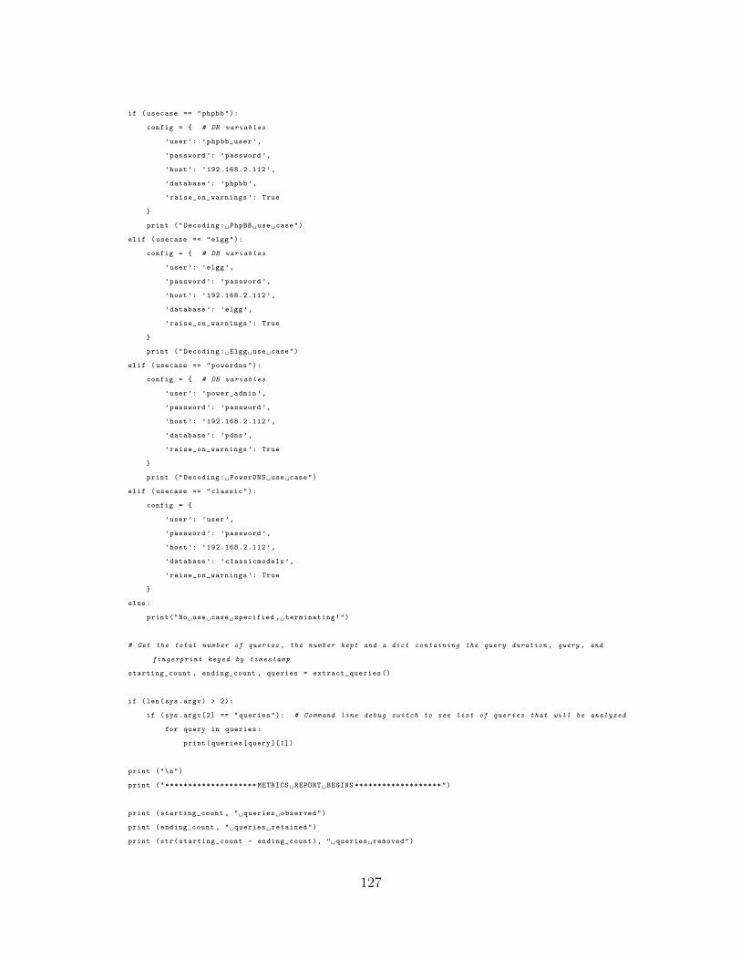
if (usecase == "phpbb"):

config = { # DB variables

’user’: ’phpbb_user ’,

’password ’: ’password ’,

’host’: ’192.168.2.112 ’,

’database ’: ’phpbb’,

’raise_on_warnings ’: True

}

print ("Decoding: PhpBB use case")

elif (usecase == "elgg"):


’user’: ’elgg’,


’host’: ’192.168.2.112 ’,

’database ’: ’elgg’,


}

print ("Decoding: Elgg use case")

elif (usecase == "powerdns"):


’user’: ’power_admin ’,


’host’: ’192.168.2.112 ’,

’database ’: ’pdns’,


}

print ("Decoding: PowerDNS use case")

elif (usecase == "classic"):

config = {

’user’: ’user’,


’host’: ’192.168.2.112 ’,

’database ’: ’classicmodels ’,


}

else:

print("No use case specified , terminating!")

# Get the total number of queries , the number kept and a dict containing the query duration , query , and

fingerprint keyed by timestamp

starting_count , ending_count , queries = extract_queries ()

if (len(sys.argv) > 2):

if (sys.argv [2] == "queries"): # Command line debug switch to see list of queries that will be analyzed


print(queries[query ][1])

print ("\n")

print ("******************** METRICS REPORT BEGINS *******************")

print (starting_count , " queries observed")

print (ending_count , " queries retained")

print (str(starting_count - ending_count), " queries removed")

127

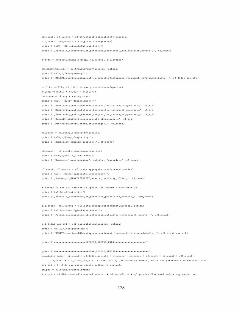
c2_count , c2_events = c2_structural_malleability(queries)

c10_count , c10_events = c10_plasticity(queries)

print ("\nC2 - Structural Malleability:")

print (" Probable occurences of potential structural malleability events: ", c2_count)

schema = extract_schema(config , c2_events , c10_events)

c3_didnt_use_all = c3_transparency(queries , schema)

print ("\nC3 - Transparency:")

print (" SELECT queries using only a subset of elements from each referenced table: ", c3_didnt_use_all)

c4_1_2 , c4_2_3 , c4_1_3 = c4_query_omniscience(queries)

c4_avg =( c4_1_2 + c4_2_3 + c4_1_3)/3

c4_score = c4_avg * ending_count

print ("\nC4 - Query Omniscience: ")

print (" Similarity ratio between 1st and 2nd thirds of queries: ", c4_1_2)

print (" Similarity ratio between 2nd and 3rd thirds of queries: ", c4_2_3)

print (" Similarity ratio between 1st and 3rd thirds of queries: ", c4_1_3)

print (" Overall similarity across all three sets: ", c4_avg)

print (" Pro -rated score based on average: ", c4_score)

c5_score = c5_query_complexity(queries)

print ("\nC5 - Query Complexity:")

print (" Number of complex queries: ", c5_score)

c6_count = c6_result_timeliness(queries)

print ("\nC6 - Result Timeliness:")

print (" Number of events under", quickly , "seconds: ", c6_count)

c7_count , c7_events = c7_cross_aggregate_consistency(queries)

print ("\nC7 - Cross -Aggregate Consistency:")

print (" Number of UPDATE/DELETE events involving JOINs: ", c7_count)

# Needed to run C10 earlier to update the schema - look near C2

print ("\nC10 - Plasticity:")

print (" Probable occurences of potential plasticity events: ", c10_count)

c11_count , c11_events = c11_data_typing_enforcement(queries , schema)

print ("\nC11 - Data Type Enforcement:")

print (" Probable occurences of potential data type enforcement events: ", c11_count)

c12_didnt_use_all = c12_manipulation(queries , schema)

print ("\nC12 - Manipulation:")

print (" UPDATE queries NOT using every element from each referenced table: ", c12_didnt_use_all)

print ("********************* METRICS REPORT ENDS *********************")

print ("\n********************** SAW OUTPUT BEGINS **********************")

counted_events = c2_count + c3_didnt_use_all + c4_score + c5_score + c6_count + c7_count + c10_count +

c11_count + c12_didnt_use_all # Count all of the observed events , so we can generate a normalized total

pre_pri = 0 # No currently viable method to evaluate

sm_pri = c2_count/counted_events

tra_pri = c3_didnt_use_all/counted_events # c3_use_all is # of queries that used entire aggregate , so

128

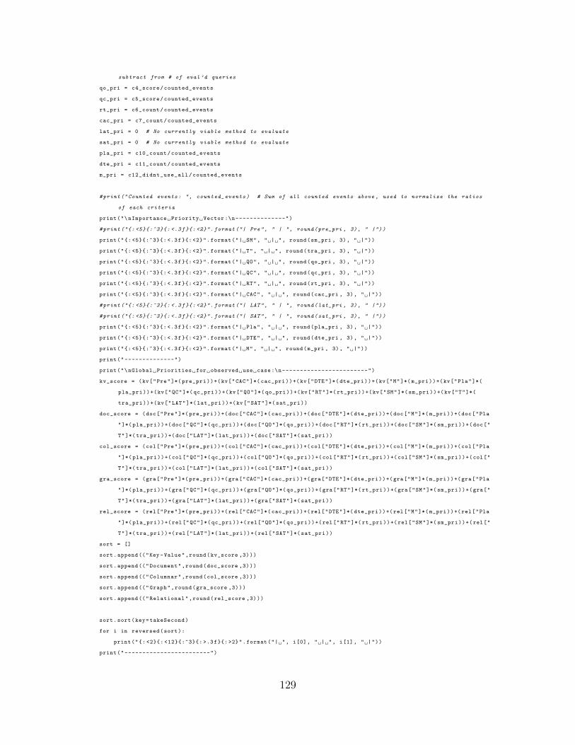
subtract from # of eval ’d queries

qo_pri = c4_score/counted_events

qc_pri = c5_score/counted_events

rt_pri = c6_count/counted_events

cac_pri = c7_count/counted_events

lat_pri = 0 # No currently viable method to evaluate

sat_pri = 0 # No currently viable method to evaluate

pla_pri = c10_count/counted_events

dte_pri = c11_count/counted_events

m_pri = c12_didnt_use_all/counted_events

#print (" Counted events: ", counted_events ) # Sum of all counted events above , used to normalize the ratios

of each criteria

print("\nImportance Priority Vector :\n--------------")

#print ("{: <5}{:^3}{: <.3f}{: <2}". format ("| Pre", " | ", round(pre_pri , 3), " |"))

print("{: <5}{:^3}{: <.3f}{: <2}".format("| SM", " | ", round(sm_pri , 3), " |"))

print("{: <5}{:^3}{: <.3f}{: <2}".format("| T", " | ", round(tra_pri , 3), " |"))

print("{: <5}{:^3}{: <.3f}{: <2}".format("| QO", " | ", round(qo_pri , 3), " |"))

print("{: <5}{:^3}{: <.3f}{: <2}".format("| QC", " | ", round(qc_pri , 3), " |"))

print("{: <5}{:^3}{: <.3f}{: <2}".format("| RT", " | ", round(rt_pri , 3), " |"))

print("{: <5}{:^3}{: <.3f}{: <2}".format("| CAC", " | ", round(cac_pri , 3), " |"))

#print ("{: <5}{:^3}{: <.3f}{: <2}". format ("| LAT", " | ", round(lat_pri , 3), " |"))

#print ("{: <5}{:^3}{: <.3f}{: <2}". format ("| SAT", " | ", round(sat_pri , 3), " |"))

print("{: <5}{:^3}{: <.3f}{: <2}".format("| Pla", " | ", round(pla_pri , 3), " |"))

print("{: <5}{:^3}{: <.3f}{: <2}".format("| DTE", " | ", round(dte_pri , 3), " |"))

print("{: <5}{:^3}{: <.3f}{: <2}".format("| M", " | ", round(m_pri , 3), " |"))

print("--------------")

print("\nGlobal Priorities for observed use case:\n------------------------")

kv_score = (kv["Pre"]*( pre_pri))+(kv["CAC"]*( cac_pri))+(kv["DTE"]*( dte_pri))+(kv["M"]*( m_pri))+(kv["Pla"]*(

pla_pri))+(kv["QC"]*( qc_pri))+(kv["QO"]*( qo_pri))+(kv["RT"]*( rt_pri))+(kv["SM"]*( sm_pri))+(kv["T"]*(

tra_pri))+(kv["LAT"]*( lat_pri))+(kv["SAT"]*( sat_pri))

doc_score = (doc["Pre"]*( pre_pri))+(doc["CAC"]*( cac_pri))+(doc["DTE"]*( dte_pri))+(doc["M"]*( m_pri))+(doc["Pla

"]*( pla_pri))+(doc["QC"]*( qc_pri))+(doc["QO"]*( qo_pri))+(doc["RT"]*( rt_pri))+(doc["SM"]*( sm_pri))+(doc["

T"]*( tra_pri))+(doc["LAT"]*( lat_pri))+(doc["SAT"]*( sat_pri))

col_score = (col["Pre"]*( pre_pri))+(col["CAC"]*( cac_pri))+(col["DTE"]*( dte_pri))+(col["M"]*( m_pri))+(col["Pla

"]*( pla_pri))+(col["QC"]*( qc_pri))+(col["QO"]*( qo_pri))+(col["RT"]*( rt_pri))+(col["SM"]*( sm_pri))+(col["

T"]*( tra_pri))+(col["LAT"]*( lat_pri))+(col["SAT"]*( sat_pri))

gra_score = (gra["Pre"]*( pre_pri))+(gra["CAC"]*( cac_pri))+(gra["DTE"]*( dte_pri))+(gra["M"]*( m_pri))+(gra["Pla

"]*( pla_pri))+(gra["QC"]*( qc_pri))+(gra["QO"]*( qo_pri))+(gra["RT"]*( rt_pri))+(gra["SM"]*( sm_pri))+(gra["

T"]*( tra_pri))+(gra["LAT"]*( lat_pri))+(gra["SAT"]*( sat_pri))

rel_score = (rel["Pre"]*( pre_pri))+(rel["CAC"]*( cac_pri))+(rel["DTE"]*( dte_pri))+(rel["M"]*( m_pri))+(rel["Pla

"]*( pla_pri))+(rel["QC"]*( qc_pri))+(rel["QO"]*( qo_pri))+(rel["RT"]*( rt_pri))+(rel["SM"]*( sm_pri))+(rel["

T"]*( tra_pri))+(rel["LAT"]*( lat_pri))+(rel["SAT"]*( sat_pri))

sort = []

sort.append (("Key -Value",round(kv_score ,3)))

sort.append (("Document",round(doc_score ,3)))

sort.append (("Columnar",round(col_score ,3)))

sort.append (("Graph",round(gra_score ,3)))

sort.append (("Relational",round(rel_score ,3)))

sort.sort(key=takeSecond)

for i in reversed(sort):

print("{: <2}{: <12}{:^3}{: >.3f}{:>2}".format("| ", i[0], " | ", i[1], " |"))

print("------------------------")

129

print ("*********************** SAW OUTPUT ENDS ***********************")

return datetime.datetime.now(), ending_count , round(rel_score , 5), round(kv_score , 5), round(doc_score , 5),

round(col_score , 5), round(gra_score , 5)

if __name__ == ’__main__ ’:

sys.exit(main(sys.argv [1]))

130

Appendix B. classic agent image.py code

#!/ usr/bin/python3

# File: classic_agent_image .py


# This script simulates a user interactinfg with the " classicmodels " sample SQL database.

# https :// www. mysqltutorial .org/getting -started -with -mysql/mysql -sample -database -aspx/


import sys

import glob

import random

import string

import os

import time

import base64

from mysql.connector import Error

from loremipsum import get_sentences


’user’: ’user’,


’host’: ’192.168.2.112 ’,

’database ’: ’classicmodels ’,


}

def convertToBinaryData(filename):

with open(filename , ’rb’) as file:

binaryData = file.read()

return binaryData

def writeToFile(filename , photo):

savePath = os.path.join("/home/labuser/Pictures/output", filename)

print("Saving to: ", savePath)

with open(savePath , ’wb’) as f:

f.write(base64.b64decode(photo))

def trigger_relational(cnx):

iterations = 50

customers = get_customers(cnx)


try:

cursor.execute("DROP TABLE IF EXISTS persons")

except mysql.connector.errors.DatabaseError:

pass

cursor.execute("CREATE TABLE persons (PhotoID int PRIMARY KEY , modified int (1), customerNumber int (11), photo

LONGBLOB , FOREIGN KEY (customerNumber) REFERENCES customers(customerNumber));")

cnx.commit ()

cursor.execute("ALTER TABLE persons MODIFY PhotoID int (11) NOT NULL AUTO_INCREMENT") # Trigger DTE by

specifying int field constraints

cnx.commit ()

cursor.execute("ALTER TABLE persons MODIFY photo LONGBLOB NOT NULL") # Trigger DTE again

cnx.commit ()

131

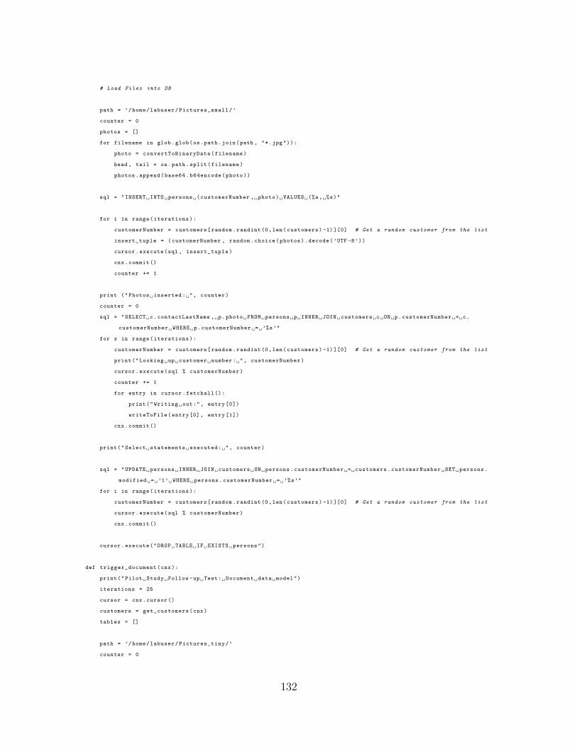
# Load Files into DB

path = ’/home/labuser/Pictures_small/’

counter = 0

photos = []

for filename in glob.glob(os.path.join(path , "*.jpg")):

photo = convertToBinaryData(filename)

head , tail = os.path.split(filename)

photos.append(base64.b64encode(photo))

sql = "INSERT INTO persons (customerNumber , photo) VALUES (%s, %s)"

for i in range(iterations):

customerNumber = customers[random.randint(0,len(customers) -1)][0] # Get a random customer from the list

insert_tuple = (customerNumber , random.choice(photos).decode(’UTF -8’))

cursor.execute(sql , insert_tuple)

cnx.commit ()

counter += 1

print ("Photos inserted: ", counter)

counter = 0

sql = "SELECT c.contactLastName , p.photo FROM persons p INNER JOIN customers c ON p.customerNumber = c.

customerNumber WHERE p.customerNumber = ’%s’"

for x in range(iterations):


print("Looking up customer number: ", customerNumber)

cursor.execute(sql % customerNumber)

counter += 1

for entry in cursor.fetchall ():

print("Writing out:", entry [0])

writeToFile(entry[0], entry [1])

cnx.commit ()

print("Select statements executed: ", counter)

sql = "UPDATE persons INNER JOIN customers ON persons.customerNumber = customers.customerNumber SET persons.

modified = ’1’ WHERE persons.customerNumber = ’%s’"



cursor.execute(sql % customerNumber)

cnx.commit ()


def trigger_document(cnx):

print("Pilot Study Follow -up Test: Document data model")

iterations = 25



tables = []

path = ’/home/labuser/Pictures_tiny/’

counter = 0

132

photos = []





for i in range(iterations *2): # Create a bunch of tables

table = randomString ().strip ()

entry = [table , ["Photo", "PersonID", "customerNumber", "neverUsed"]]

tables.append(entry)

cursor.execute("CREATE TABLE %s (Photo LONGBLOB , PersonID blob , customerNumber int (11), neverUsed blob ,

FOREIGN KEY (customerNumber) REFERENCES customers(customerNumber));" % table)

cnx.commit ()

for i in range(iterations *2): # Modify the tables to add a bunch of columns

table = tables.pop(random.randint(0,len(tables) -1)) # Remove a random element from the list

elements = random.randint (5,15) # Choose between 5 and 15 new columns to create

for j in range(elements):

column = randomString ().strip ()

cursor.execute("ALTER TABLE %s ADD %s BLOB" % (table[0], column))

cnx.commit ()

table [1]. append(column)

tables.append(table)

print (tables)

for i in range(iterations): # Insert some data into the database

table = tables.pop(random.randint(0,len(tables) -1)) # Get a random table from the list

elements = random.randint(3,len(table [1])) # Select the number of columns to pull from the table

columns = []

data = []


print(j)

columns.append(table [1][j])

for k in range(elements +1):

if k == 1:

data.append(random.choice(photos).decode(’UTF -8’)) # Insert a random photo

elif k == 3:

data.append(customers[random.randint(0,len(customers) -1)][0]) # Insert a random customer number

else:

data.append(randomString ()*k*k) # Create some text data to be stored

data.pop(0)

if (elements == 3):

cursor.execute("INSERT INTO %s (%s, %s, %s) VALUES (’%s’, ’%s’, ’%s ’);" % (table[0], columns [0],

columns [1], columns [2], data[0], data[1], data [2]))

elif (elements == 4):

cursor.execute("INSERT INTO %s (%s, %s, %s, %s) VALUES (’%s’, ’%s’, ’%s’, ’%s ’);" % (table [0],

columns [0], columns [1], columns [2], columns [3], data[0], data[1], data[2], data [3]))


cursor.execute("INSERT INTO %s (%s, %s, %s, %s, %s) VALUES (’%s’, ’%s’, ’%s’, ’%s’, ’%s ’);" % (table

[0], columns [0], columns [1], columns [2], columns [3], columns [4], data[0], data[1], data[2], data

[3], data [4]))


cursor.execute("INSERT INTO %s (%s, %s, %s, %s, %s, %s) VALUES (’%s’, ’%s’, ’%s’, ’%s’, ’%s’, ’%s’);"

133

% (table [0], columns [0], columns [1], columns [2], columns [3], columns [4], columns [5], data[0],

data[1], data[2], data[3], data[4], data [5]))


cursor.execute("INSERT INTO %s (%s, %s, %s, %s, %s, %s, %s) VALUES (’%s’, ’%s’, ’%s’, ’%s’, ’%s’, ’%s

’, ’%s ’);" % (table[0], columns [0], columns [1], columns [2], columns [3], columns [4], columns [5],

columns [6], data[0], data[1], data[2], data[3], data[4], data[5], data [6]))

else:

cursor.execute("INSERT INTO %s (%s, %s, %s, %s, %s, %s, %s, %s) VALUES (’%s’, ’%s’, ’%s’, ’%s’, ’%s’,

’%s’, ’%s’, ’%s ’);" % (table [0], columns [0], columns [1], columns [2], columns [3], columns [4],

columns [5], columns [6], columns [7], data[0], data[1], data[2], data[3], data[4], data[5], data

[6], data [7]))

cnx.commit ()

print("Inserting data: ", data [0])


for i in range(iterations): # Select some data from the database

table = tables.pop(random.randint(0,len(tables) -1)) # Remove a random element from the list

elements = random.randint(3,len(table [1])) # Select the number of columns to pull from the table (there

should be at least 3 in every table)

columns = []


columns.append(table [1][j]) # TODO: Should check to make sure it isn ’t already used

if (elements == 1):

cursor.execute("SELECT x.%s, c.phone FROM %s x INNER JOIN customers c ON x.customerNumber = c.

customerNumber" % (columns [0], table [0]))


cursor.execute("SELECT x.%s, x.%s, c.phone FROM %s x INNER JOIN customers c ON x.customerNumber = c.

customerNumber" % (columns [0], columns [1], table [0]))


cursor.execute("SELECT x.%s, x.%s, x.%s, c.phone FROM %s x INNER JOIN customers c ON x.customerNumber

= c.customerNumber" % (columns [0], columns [1], columns [2], table [0]))


cursor.execute("SELECT x.%s, x.%s, x.%s, x.%s, c.phone FROM %s x INNER JOIN customers c ON x.

customerNumber = c.customerNumber" % (columns [0], columns [1], columns [2], columns [3], table [0]))


cursor.execute("SELECT x.%s, x.%s, x.%s, x.%s, x.%s, c.phone FROM %s x INNER JOIN customers c ON x.

customerNumber = c.customerNumber" % (columns [0], columns [1], columns [2], columns [3], columns

[4], table [0]))


cursor.execute("SELECT x.%s, x.%s, x.%s, x.%s, x.%s, x.%s, c.phone FROM %s x INNER JOIN customers c

ON x.customerNumber = c.customerNumber" % (columns [0], columns [1], columns [2], columns [3],

columns [4], columns [5], table [0]))


cursor.execute("SELECT x.%s, x.%s, x.%s, x.%s, x.%s, x.%s, x.%s, c.phone FROM %s x INNER JOIN

customers c ON x.customerNumber = c.customerNumber" % (columns [0], columns [1], columns [2],

columns [3], columns [4], columns [5], columns [6], table [0]))

else:

cursor.execute("SELECT x.%s, x.%s, x.%s, x.%s, x.%s, x.%s, x.%s, x.%s, c.phone FROM %s x INNER JOIN

customers c ON x.customerNumber = c.customerNumber" % (columns [0], columns [1], columns [2],

columns [3], columns [4], columns [5], columns [6], columns [7], table [0]))

for row in cursor.fetchall ():

print(row)


134

for table in tables: # Clean up

cursor.execute("DROP TABLE IF EXISTS %s;" % table [0])

def trigger_graph(cnx):

iterations = 50



path = ’/home/labuser/Pictures_tiny/’

photos = []

for filename in glob.glob(os.path.join(path , "*.jpg")): # Load photos into data structure




try:



pass

cursor.execute("CREATE TABLE persons (photo LONGBLOB , PersonID int , LastName varchar (255) , customerNumber int

(11), FOREIGN KEY (customerNumber) REFERENCES customers(customerNumber));")


PID = random.randint (1 ,100000)

cursor.execute("ALTER TABLE persons DROP LastName;")

cursor.execute("ALTER TABLE persons ADD LastName varchar (255);")

cursor.execute("ALTER TABLE persons ADD NickName varchar (255);")

cursor.execute("ALTER TABLE persons DROP NickName;")

cursor.execute("INSERT INTO persons (photo , PersonID , customerNumber , LastName) VALUES (’%s’, 1, ’%s’, ’

Smith ’);" % (random.choice(photos).decode(’UTF -8’), customers[random.randint(0,len(customers) -1)

][0]))


cursor.execute("UPDATE persons INNER JOIN customers ON persons.customerNumber = customers.customerNumber

set persons.LastName = customers.contactLastName WHERE persons.LastName LIKE ’Sm%’")

cursor.execute("SELECT p.LastName , c.phone FROM persons p INNER JOIN customers c ON p.customerNumber = c.

customerNumber WHERE p.LastName LIKE ’S%’ ORDER BY RAND()")

cursor.fetchall ()

cursor.execute("UPDATE persons INNER JOIN customers ON persons.customerNumber = customers.customerNumber

set persons.LastName = customers.contactLastName WHERE persons.LastName LIKE ’Sm%’")

cnx.commit ()


def trigger_column(cnx):

iterations = 25




photos = []

for filename in glob.glob(os.path.join(path , "*.jpg")): # Load photos into data structure




try:


135


pass

cursor.execute("CREATE TABLE persons (photo LONGBLOB , PersonID int , customerNumber int (11), FOREIGN KEY (

customerNumber) REFERENCES customers(customerNumber));")


cursor.execute("ALTER TABLE persons ADD LastName varchar (255);")

cursor.execute("ALTER TABLE persons ADD NickName varchar (255);")


Smith ’);" % (random.choice(photos).decode(’UTF -8’), customers[random.randint(0,len(customers) -1)

][0]))


Beach ’);" % (random.choice(photos).decode(’UTF -8’), customers[random.randint(0,len(customers) -1)

][0]))

cursor.execute("UPDATE persons set LastName = ’Smithy ’ WHERE LastName LIKE ’Sm%’")

cnx.commit ()

cursor.execute("SELECT photo , customerNumber FROM persons WHERE LastName LIKE ’Smit%’")

cursor.fetchall ()

cursor.execute("ALTER TABLE persons DROP LastName;")

cursor.execute("ALTER TABLE persons DROP NickName;")


def randomString(stringLength =12): # pynative.com/python -generate -random -string/

letters = string.ascii_lowercase

return ’’.join(random.choice(letters) for i in range(stringLength))

def trigger_key_value(cnx):

customers = get_customers(cnx) # Get list of valid customer id’s



try:



pass

cursor.execute("CREATE TABLE persons (customerNumber int , photo LONGBLOB , FOREIGN KEY (customerNumber)

REFERENCES customers(customerNumber));")

cnx.commit ()

usedNumbers = [] # Place to store the numbers that were actually used




cursor.execute("INSERT INTO persons (customerNumber , photo) VALUES (’%s’, ’%s ’);" % (customerNumber ,

base64.b64encode(photo).decode(’utf -8’)))

cnx.commit ()

usedNumbers.append(customerNumber)

for i in range (200):

custNum = usedNumbers[random.randint(0,len(usedNumbers) -1)] # Super not pythonic

cursor.execute("SELECT * FROM persons WHERE customerNumber = ’%s ’;" % custNum)

cursor.fetchall ()

136

cnx.commit ()


def get_customers(cnx):


cursor.execute("SELECT customerNumber FROM customers")

customers = []

for customer in cursor.fetchall (): # Get a list of all the customers in the db

customers.append(customer)

return customers

def main(datamodel):


if (datamodel == "col"):

trigger_column(cnx)

elif (datamodel == "gra"):

trigger_graph(cnx)

elif (datamodel == "rel"):

trigger_relational(cnx)

elif (datamodel == "doc"):

trigger_document(cnx)

elif (datamodel == "kv"):

trigger_key_value(cnx)

else:

print("ERROR: No data model specified. Exiting.")

if __name__ == ’__main__ ’:

sys.exit(main(sys.argv [1]))

137

Appendix C. phpbb agent.py code

#!/ usr/bin/python3

# File: agent.py

# Date: 4 Sept 19


# This script simulates a user browsing the phpbb web application

from __future__ import print_function

import random , time

from selenium import webdriver

from loremipsum import get_sentences

import re

import sys

def eprint (*args , ** kwargs):

print(*args , file=sys.stderr , ** kwargs)

def fix_loremipsum(loremipsum_string): # Fix issue in loremipsum library

# From https :// stackoverflow .com/questions /50133478/ byte -prefix -in -python -string

loremipsum_string = re.sub("B ’(.*?)’", lambda x: x.group (1).title(), loremipsum_string)

loremipsum_string = re.sub("b ’(.*?)’", lambda x: x.group (1), loremipsum_string)

return loremipsum_string

def login(driver):

# Open the website

print("Opening browser ...")

driver.get(’http ://192.168.2.114 ’)

time.sleep (.5)

# Find the username and password boxes , enter the data and submit

print("Logging in...")

time.sleep (1.5)

id_box = driver.find_element_by_id(’username ’)

id_box.send_keys(’admin ’)

pass_box = driver.find_element_by_id(’password ’)

pass_box.send_keys(’password ’)

login_button = driver.find_element_by_name(’login’)

login_button.click ()

def logout(driver): # Close the browser to clear the session

print("Closing browser ...")

driver.close()

time.sleep (1.5)

def read_subforum(driver):

# Select an existing subforum and enter it

print("Entering subforum ...")

time.sleep (1.5)

forum = driver.find_element_by_link_text(’Your first forum’)

forum.click ()

def new_thread(driver):

# Create a new topic

138

print("Creating topic ...")

subject = "Random thread from agent.py: #" + str(random.randint (10000 ,99999)) #Generate random subject number

sentences = get_sentences (6, False) #Generate random message text

text = ’’

for i in sentences:

text = text + ’ ’ + fix_loremipsum(i)

time.sleep (1.5)

driver.get("http ://192.168.2.114/ posting.php?mode=post&f=2")

subject_box = driver.find_element_by_id(’subject ’)

subject_box.send_keys(subject)

message_box = driver.find_element_by_id(’message ’)

message_box.send_keys(text)

submit_button = driver.find_element_by_name(’post’)

submit_button.click()

def read_thread(driver):

driver.get(’http ://192.168.2.114/ viewtopic.php?f=2&t=’+ str(random.randint (1 ,1276)))

def new_comment(driver):

read_thread(driver)

print("Creating comment ...")

time.sleep (1.5)

sentences = get_sentences (6, False) #Generate random message text

text = ’’

for i in sentences:


time.sleep (1.5)

new_post = driver.find_element_by_link_text(’Post Reply ’)

new_post.click()

message_box = driver.find_element_by_id(’message ’)

message_box.send_keys(text)

submit_button = driver.find_element_by_name(’post’)


def main():

seed = sys.argv [1]

random.seed(seed)

driver = webdriver.Chrome ()

login(driver)

actions_to_complete = random.randint (30 ,40) # Set the duration of the user session between 30 and 40 actions

num_comments = round(actions_to_complete * random.uniform (.1, .3)) # Default values: .01 - .03

num_threads = round(actions_to_complete * random.uniform (.1, .3)) # Default values: .01 - .03

num_subforum_reads = round(actions_to_complete * random.uniform (.10, .15)) # Default values: .10 - .20

num_thread_reads = actions_to_complete - num_comments - num_threads - num_subforum_reads

print("Actions to complete: ", actions_to_complete + 2)

print("Subforums to read: ", num_subforum_reads)

print("Threads to read: ", num_thread_reads)

print("Threads to create: ", num_threads)

print("Comments to create: ", num_comments)

if (num_thread_reads < 1):

num_thread_reads = 1

139

if (num_subforum_reads < 1):

num_subforum_reads = 1

read_subforum(driver) # Need to start off with opening the subforum

for x in range(num_threads): # If we’re going to make a new post , now is a good time

new_thread(driver)

for x in range(num_subforum_reads - 1):

read_subforum(driver)

read_thread(driver) # Need to read a thread to post

for x in range (num_comments):

new_comment(driver)

for x in range(num_thread_reads - 1):

read_thread(driver)

logout(driver)

eprint (actions_to_complete + 2) # Send number of completed actions to stderr (include log in and log out)

print (actions_to_complete + 2)

print("Totals:", str(int(actions_to_complete + 2)), ",", str(num_subforum_reads), ",", str(num_thread_reads),

",", str(num_threads), ",", str(num_comments))

main()

140

Appendix D. elgg agent.py code

#!/ usr/bin/python3

# File: elgg_agent .py

# Date: 23 Mar 20


# This script simulates a user browsing the Elgg web application

from __future__ import print_function

import random , time


import re

import sys

from selenium.webdriver.chrome.options import Options

from selenium import webdriver

from selenium.webdriver.common.by import By

from selenium.webdriver.support.ui import WebDriverWait

from selenium.webdriver.support import expected_conditions as EC

from selenium.webdriver.common.action_chains import ActionChains

from selenium.common.exceptions import NoSuchElementException

from loremipsum import generate_paragraph , get_sentences


’user’: ’elgg’,


’host’: ’192.168.2.112 ’,

’database ’: ’elgg’,


}

def eprint (*args , ** kwargs):

print(*args , file=sys.stderr , ** kwargs)

def enumerate_users (): # Query DB to enumerate all current users



cursor.execute("SELECT username FROM elgg_users_entity")

users = []

for user in cursor.fetchall (): # Get a list of all the table names in the db

users.append(user [0]) # Store the set in a dict with the table name as the key

return users

def find_friends(user , driver):

friends = []

driver.get(’http ://192.168.2.115/ friendsof/’ + user)

print("Finding friends of " + user)

more = True # Bool to determine if there are additional friends to find , assume true at start

while (more):

for x in range (10):

try:

iterator = ’/html/body/div [1]/ div [5]/ div/div/div [1]/ul[1]/li[’ + str(x + 1) + ’]/div/div [2]/h3/a’

friend = driver.find_element_by_xpath(iterator)

print ("Friend of " + user + ": " + friend.text)

if ("Admin" in friend.text): # Catch case where admin is in friends list

141

friends.append("admin")

else:

number = friend.text.split(" ")[-1]# Parse out username

parsed_name = "labuser" + number

friends.append(parsed_name)

except NoSuchElementException: # End of list found

break

try:

next_btn = driver.find_element_by_partial_link_text("Next") # load next page

next_btn.click()

except NoSuchElementException:

more = False # Already on last page , stop working

return friends

def fix_loremipsum(loremipsum_string): # Fix issue in loremipsum library

# From https :// stackoverflow .com/questions /50133478/ byte -prefix -in -python -string

loremipsum_string = re.sub("B ’(.*?)’", lambda x: x.group (1).title(), loremipsum_string)

loremipsum_string = re.sub("b ’(.*?)’", lambda x: x.group (1), loremipsum_string)

return loremipsum_string

def login(user , driver): # Log a user in (only need username , password always ’password ’)

print ("Logging in: " + user)

try:

id_box = driver.find_element_by_xpath(’/html/body/div [1]/ div [4]/ div/div/div [2]/ div/div [2]/ form/fieldset/

div [1]/ input ’)

id_box.send_keys(user)

pass_box = driver.find_element_by_xpath(’/html/body/div [1]/ div [4]/ div/div/div [2]/ div/div [2]/ form/fieldset

/div [2]/ input ’)

pass_box.send_keys(’password ’)

login_button = driver.find_element_by_xpath(’/html/body/div [1]/ div [4]/ div/div/div [2]/ div/div [2]/ form/

fieldset/div [3]/ div/input ’)

login_button.click ()

except NoSuchElementException: # Already logged in

print("Error logging in... user already logged in")

def make_friends(user1 , user2 , driver):

login(user1 , driver)

driver.get(’http ://192.168.2.115/ profile/’ + user2)

print ("Making friends: " + user1 + ’ and ’ + user2)

try:

add_friend_button = driver.find_element_by_link_text(’Add friend ’)

add_friend_button.click()

except NoSuchElementException:

print ("Error , " + user1 + " and " + user2 + "are already friends. Skipping.")

def open_session (): # Opens a new connection

options = webdriver.ChromeOptions ()

options.add_argument("window -size =1920 x1080")

options.add_experimental_option("excludeSwitches", ["enable -automation"])

options.add_experimental_option(’useAutomationExtension ’, False)

driver = webdriver.Chrome(options=options)

driver.get(’http ://192.168.2.115 ’) # Open the website

return driver

142

def new_comment(driver): # Generates a random comment to an existing thread

driver.get(’http ://192.168.2.115/ activity ’)

last_page = driver.find_element_by_xpath("//a[contains(text(),’Next ’)]/../ preceding -sibling ::li[1]/a") #

Find button before last page

href = last_page.get_attribute(’href’)

page_count = int(href.split(’=’, 1)[-1]. rstrip(’#’)) # Strip the url that looks like http ://192.168.2.115/

activity?offset =220# to just the number

select_page = random.randint(1,page_count -20) # Chose a random page from the activity list , skip last page

to avoid guessing at non -existent topic

driver.get(’http ://192.168.2.115/ activity?offset=’ + str(select_page) + ’#’) # Load that page of topics

random_topic = driver.find_element_by_xpath(’/html/body/div [1]/ div [5]/ div/div/div [1]/ul[2]/li[’ + str(random.

randint (1,20)) + ’]/div/div [2]/ div [1]/a[2]’)

while("http ://192.168.2.115/ profile" in random_topic.get_attribute(’href’)): # Make sure it is a page that

can be commented on

select_page = random.randint(1,page_count -20) # Chose a random page from the activity list , skip last

page to avoid guessing at non -existent topic

print(’http ://192.168.2.115/ activity?offset=’ + str(select_page) + ’#’)

driver.get(’http ://192.168.2.115/ activity?offset=’ + str(select_page) + ’#’) # Load that page of topics

random_topic = driver.find_element_by_xpath(’/html/body/div [1]/ div [5]/ div/div/div [1]/ul[2]/li[’ + str(

random.randint (1 ,20)) + ’]/div/div [2]/ div [1]/a[2]’)

random_topic.click ()

sentences = get_sentences (2, True) # Generate lorem ipsum text

text = ’’

print ("Creating comment")

for i in sentences:


WebDriverWait(driver , 20).until(EC.visibility_of_element_located ((By.TAG_NAME , "iframe")))

driver.switch_to.frame(driver.find_element_by_tag_name("iframe")) # Find the iframe

text_box = driver.find_element_by_xpath(’/html/body/p’)

text_box.send_keys(text)

driver.switch_to.default_content ()

submit_button = driver.find_element_by_xpath(’/html/body/div [1]/ div [5]/ div/div/div [1]/ div [3]/ form/fieldset/

div [2]/ input [2]’)


def new_page(driver):

title = "Random page from elgg_agent.py: #" + str(random.randint (10000 ,99999)) # Generate random title

number

sentences = get_sentences (6, True) # Generate lorem ipsum text

text = ’’

for i in sentences:


print ("Creating page: " + title)

driver.get(’http ://192.168.2.115/ pages/all’)

add_page_button = driver.find_element_by_link_text(’Add a page’)

add_page_button.click ()

title_box = driver.find_element_by_xpath(’/html/body/div [1]/ div [5]/ div/div/div [1]/ form/fieldset/div [1]/ input’

)

title_box.send_keys(title)

WebDriverWait(driver , 20).until(EC.visibility_of_element_located ((By.TAG_NAME , "iframe")))

driver.switch_to.frame(driver.find_element_by_tag_name("iframe")) # Find the iframe

text_box = driver.find_element_by_xpath(’/html/body/p’)

text_box.send_keys(text)

driver.switch_to.default_content ()

143

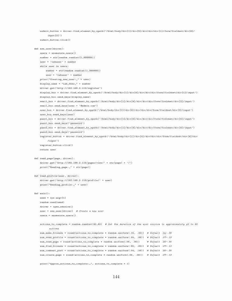
submit_button = driver.find_element_by_xpath(’/html/body/div [1]/ div [5]/ div/div/div [1]/ form/fieldset/div [6]/

input [3]’)


def new_user(driver):

users = enumerate_users ()

number = str(random.randint (1 ,999999))

user = ’labuser ’ + number

while user in users:

number = str(random.randint (1 ,999999))

user = ’labuser ’ + number

print("Creating new user: " + user)

display_name = "Lab User " + number

driver.get(’http ://192.168.2.115/ register ’)

display_box = driver.find_element_by_xpath(’/html/body/div [1]/ div [4]/ div/div/div/form/fieldset/div [1]/ input’)

display_box.send_keys(display_name)

email_box = driver.find_element_by_xpath(’/html/body/div [1]/ div [4]/ div/div/div/form/fieldset/div [2]/ input’)

email_box.send_keys(user + ’@admin.com’)

user_box = driver.find_element_by_xpath(’/html/body/div [1]/ div [4]/ div/div/div/form/fieldset/div [3]/ input’)

user_box.send_keys(user)

pass1_box = driver.find_element_by_xpath(’/html/body/div [1]/ div [4]/ div/div/div/form/fieldset/div [4]/ input’)

pass1_box.send_keys(’password ’)

pass2_box = driver.find_element_by_xpath(’/html/body/div [1]/ div [4]/ div/div/div/form/fieldset/div [5]/ input’)

pass2_box.send_keys(’password ’)

register_button = driver.find_element_by_xpath(’/html/body/div [1]/ div [4]/ div/div/div/form/fieldset/div [6]/ div

/input’)

register_button.click ()

return user

def read_page(page , driver):

driver.get(’http ://192.168.2.115/ pages/view/’ + str(page) + ’/’)

print("Reading page: " + str(page))

def read_profile(user , driver):

driver.get(’http ://192.168.2.115/ profile/’ + user)

print("Reading profile: " + user)

def main():

seed = sys.argv [1]

random.seed(seed)

driver = open_session ()

user = new_user(driver) # Create a new user

users = enumerate_users ()

actions_to_complete = random.randint (40 ,60) # Set the duration of the user session to approximately 40 to 60

actions

num_make_friends = round(actions_to_complete * random.uniform (.15, .25)) # Default .04 -.06

num_read_profile = round(actions_to_complete * random.uniform (.04, .06)) # Default .07 -.13

num_read_page = round(actions_to_complete * random.uniform (.04, .06)) # Default .25 -.35

num_find_friends = round(actions_to_complete * random.uniform (.55, .65)) # Default .07 -.13

num_comment_post = round(actions_to_complete * random.uniform (.04, .06)) # Default .25 -.35

num_create_page = round(actions_to_complete * random.uniform (.04, .06)) # Default .07 -.13

print("Approx actions to complete: ", actions_to_complete + 1)

144

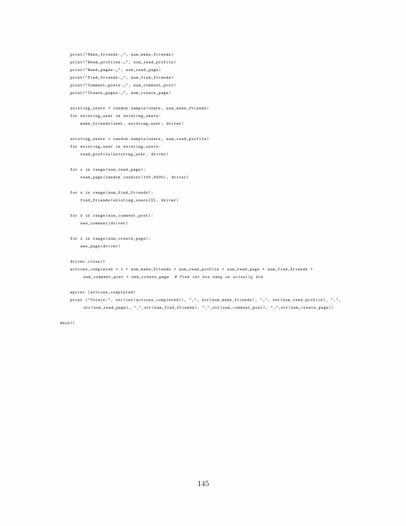
print("Make friends: ", num_make_friends)

print("Read profiles: ", num_read_profile)

print("Read pages: ", num_read_page)

print("Find friends: ", num_find_friends)

print("Comment posts: ", num_comment_post)

print("Create pages: ", num_create_page)

existing_users = random.sample(users , num_make_friends)

for existing_user in existing_users:

make_friends(user , existing_user , driver)

existing_users = random.sample(users , num_read_profile)

for existing_user in existing_users:

read_profile(existing_user , driver)

for x in range(num_read_page):

read_page(random.randint (100 ,8200), driver)

for x in range(num_find_friends):

find_friends(existing_users [0], driver)

for x in range(num_comment_post):

new_comment(driver)

for x in range(num_create_page):

new_page(driver)

driver.close()

actions_completed = 1 + num_make_friends + num_read_profile + num_read_page + num_find_friends +

num_comment_post + num_create_page # Find out how many we actually did

eprint (actions_completed)

print ("Totals:", str(int(actions_completed)), ",", str(num_make_friends), ",", str(num_read_profile), ",",

str(num_read_page), ",",str(num_find_friends), ",",str(num_comment_post), ",",str(num_create_page))

main()

145

Appendix E. powerdns agent.py code

#!/ usr/bin/python3

# File: powerdns_agent .py

# Date: 29 Mar 20


# This script simulates a user interactinfg with the PowerDNS authoritative DNS server

import os

import subprocess


import random

import string

import socket

import dns.resolver

import time


’user’: ’power_admin ’,


’host’: ’192.168.2.112 ’,

’database ’: ’pdns’,


}

def get_all_domains ():



cursor.execute("SELECT name FROM domains")

domains = []

for domain in cursor.fetchall (): # Get a list of all the table names in the db

domains.append(domain [0]) # Store the set in a dict with the table name as the key

return domains

def generate_new_domain(domains):

domain = randomString () + ’.com’

while (domain in domains): # Avoid duplicates

domain = randomString () + ’.com’

hostname = randomString () # Create some random data

ip_addr1 = str(random.randint (10 ,222)) + ’.’ + str(random.randint (0 ,254)) + ’.’ + str(random.randint (0 ,254))

+ ’.’ + str(random.randint (0 ,254))

ip_addr2 = str(random.randint (10 ,222)) + ’.’ + str(random.randint (0 ,254)) + ’.’ + str(random.randint (0 ,254))

+ ’.’ + str(random.randint (0 ,254))

print ("Inserting new domain: " + domain)

command = ’pdnsutil create -zone ’ + domain + ’ ns1.’ + domain

os.system(command)

command = ’pdnsutil add -record ’ + domain + ’ ns1 A ’ + ip_addr1

os.system(command)

command = ’pdnsutil add -record ’ + domain + ’ ’ + hostname + ’ A ’ + ip_addr2

os.system(command)

command = ’pdnsutil add -record ’ + domain + ’ @ MX "10 mx.’ + hostname + ’"’

os.system(command)

domains.append(domain)

return domains

146

def query_random_domain(domains):

domain = random.sample(domains , 1)

os.system(’dig axfr ’ + domain [0] + ’ @127 .0.0.1 ’)

def randomString(stringLength =8): # https :// pynative.com/python -generate -random -string/

""" Generate a random string of fixed length """

letters = string.ascii_lowercase

return ’’.join(random.choice(letters) for i in range(stringLength))

def main():

domains = get_all_domains ()


domains = generate_new_domain(domains)

time.sleep (.5)


query_random_domain(domains)

time.sleep (.5)

main()

147

Bibliography

Afshari, A., Mojahed, M., & Yusuff, R. M. (2010). Simple Additive Weighting ap-proach to Personnel Selection problem. International Journal of Innovation,1 (5), 5.

Allen, M. (2015). RDBMS Are Not Designed for Heterogeneous Data. RetrievedSeptember 17, 2019, from https : / / www . marklogic . com / blog / relational -databases-heterogeneous-data/

Baker, M. (2011). Search vs. Query. Retrieved September 3, 2019, from https ://everypageispageone.com/2011/07/13/search-vs-query/

Beach, P. M., Langhals, B. T., Grimaila, M. R., Hodson, D. D., & Engle, R. D. L.(2019). Developing a Methodology for the Identification of Alternative NoSQLData Models via Observation of Relational Database Usage, In Proceedings ofthe The 18th Int’l Conf on Information & Knowledge Engineering.

Burr, L., & Spennemann, D. H. (2004). Patterns of User Behavior in University On-line Forums. International Journal of Instructional Technology and DistanceLearning, 1 (10), 11–28.

Cao, Q., Liang, Z., Fan, Y., & Meng, X. (2012). A Flash-Based Decomposition StorageModel (D. Hutchison, T. Kanade, J. Kittler, J. M. Kleinberg, F. Mattern, J. C.Mitchell, M. Naor, O. Nierstrasz, C. Pandu Rangan, B. Steffen, M. Sudan, D.Terzopoulos, D. Tygar, M. Y. Vardi, G. Weikum, H. Yu, G. Yu, W. Hsu, Y.-S.Moon, . . . J. Yoo, Eds.). In D. Hutchison, T. Kanade, J. Kittler, J. M. Klein-berg, F. Mattern, J. C. Mitchell, M. Naor, O. Nierstrasz, C. Pandu Rangan,B. Steffen, M. Sudan, D. Terzopoulos, D. Tygar, M. Y. Vardi, G. Weikum, H.Yu, G. Yu, W. Hsu, Y.-S. Moon, . . . J. Yoo (Eds.), Database Systems for Ad-vanced Applications. Berlin, Heidelberg, Springer Berlin Heidelberg. RetrievedSeptember 15, 2019, from http://link.springer.com/10.1007/978-3-642-29023-7 8

Chang, F., Dean, J., Ghemawat, S., Hsieh, W. C., Wallach, D. A., Burrows, M., Chan-dra, T., Fikes, A., & Gruber, R. E. (2008). Bigtable: A Distributed StorageSystem for Structured Data. ACM Transactions on Computer Systems, 26 (2),1–26. Retrieved January 9, 2019, from http://portal.acm.org/citation.cfm?doid=1365815.1365816

Codd, E. F. (1970). A relational model of data for large shared data banks. Com-munications of the ACM, 13 (6), 377–387. Retrieved February 27, 2019, fromhttp://portal.acm.org/citation.cfm?doid=362384.362685

148

https://www.marklogic.com/blog/relational-databases-heterogeneous-data/

https://www.marklogic.com/blog/relational-databases-heterogeneous-data/

https://everypageispageone.com/2011/07/13/search-vs-query/

https://everypageispageone.com/2011/07/13/search-vs-query/

http://link.springer.com/10.1007/978-3-642-29023-7_8


http://portal.acm.org/citation.cfm?doid=1365815.1365816



Cooper, M. D. (2001). Usage Patterns of a Web-Based Library Catalog. Journal ofthe American Society for Information Science and Technology, 52 (2), 137–148.

Copeland, G., & Khoshafian, S. (1985). A Decomposition Storage Model. ACM SIG-MOD Record, 14 (4), 268–279.

DeCandia, G., Hastorun, D., Jampani, M., Kakulapati, G., Lakshman, A., Pilchin, A.,Sivasubramanian, S., Vosshall, P., & Vogels, W. (2007). Dynamo: Amazon’sHighly Available Key-value Store, 16.

Dugane, R. A., & Raut, A. B. (2014). A Survey on Big Data in Real Time. Interna-tional Journal on Recent and Innovation Trends in Computing and Commu-nication, 2 (4), 4.

Elmasri, R., & Navathe, S. (2016). Fundamentals of database systems (Seventh edi-tion). Hoboken, NJ, Pearson.

Engle, R. D. L. (2018). A Methodology for Evaluating Relational and NoSQL Databasesfor Small-scale Storage and Retrieval (Doctoral dissertation). Air Force Insti-tute of Technology.

Engle, R. D. L., Langhals, B. T., Grimaila, M. R., & Hodson, D. D. (2018). TheCase for NoSQL on a Single Desktop, In Proceedings of the 17th Int’l Conf onInformation & Knowledge Engineering, Las Vegas, NV, CSREA Press.

Evans, E. (2009). NoSQL: What’s in a name? Retrieved September 8, 2019, fromhttp://blog.sym-link.com/posts/2009/30/nosql whats in a name/

Gandomi, A., & Haider, M. (2015). Beyond the hype: Big data concepts, methods, andanalytics. International Journal of Information Management, 35 (2), 137–144.Retrieved January 9, 2019, from https://linkinghub.elsevier.com/retrieve/pii/S0268401214001066

Hecht, R., & Jablonski, S. (2011). NoSQL evaluation: A use case oriented survey,In 2011 International Conference on Cloud and Service Computing, HongKong, China, IEEE. Retrieved May 12, 2019, from http:// ieeexplore . ieee .org/document/6138544/

Hernandez, M. J. (1997). Database Design for Mere Mortals: A Hands-On Guide toRelational Database Design. Reading, Massachusetts, Addison-Wesley Devel-opers Press.

Jaccard, P. (1912). The Distribution of the Flora in the Alpine Zone.1. New Phytol-ogist, 11 (2), 37–50. Retrieved April 20, 2020, from https://nph.onlinelibrary.wiley.com/doi/abs/10.1111/j.1469-8137.1912.tb05611.x

149

http://blog.sym-link.com/posts/2009/30/nosql_whats_in_a_name/

https://linkinghub.elsevier.com/retrieve/pii/S0268401214001066


http://ieeexplore.ieee.org/document/6138544/

http://ieeexplore.ieee.org/document/6138544/

https://nph.onlinelibrary.wiley.com/doi/abs/10.1111/j.1469-8137.1912.tb05611.x

https://nph.onlinelibrary.wiley.com/doi/abs/10.1111/j.1469-8137.1912.tb05611.x

Khazaei, H., Litoiu, M., Gaikwad, P., Shtern, M., Ramprasad, B., Beigi-Mohammadi,N., Zareian, S., & Fokaefs, M. (2016). How do I choose the right NoSQLsolution? A comprehensive theoretical and experimental survey. Big Data andInformation Analytics, 1 (2/3), 185–216. Retrieved May 12, 2019, from http://www.aimsciences.org/journals/displayArticlesnew.jsp?paperID=12989

Kleppmann, M. (2017). Designing Data-Intensive Applications: The Big Ideas BehindReliable, Scalable, and Maintainable Systems. Sebastapol, CA, O’Reilly Media.

Lu, J., Liu, Z. H., Xu, P., & Zhang, C. (2018). UDBMS: Road to Unification forMulti-model Data Management, XI’an, China, Springer.

McCreary, D., & Kelly, A. (2014). Making sense of NoSQL: A guide for managersand the rest of us. Shelter Island, Manning.

Melton, J. (2003). ISO/IEC 9075-2:2016 (SQL/foundation). ISO standard.

mysqltutorial.org. (2020). MySQL Sample Database. Retrieved June 26, 2020, fromhttps://www.mysqltutorial.org/mysql-sample-database.aspx/

NIST Big Data Public Working Group Definitions and Taxonomies Subgroup. (2015).NIST Big Data Interoperability Framework: Volume 1, Definitions (tech. rep.NIST SP 1500-1). National Institute of Standards and Technology. RetrievedJanuary 9, 2019, from https://nvlpubs.nist.gov/nistpubs/SpecialPublications/NIST.SP.1500-1.pdf

Percona, LLC. (2019). Percona Toolkit. Retrieved September 4, 2019, from https://www.percona.com/software/database-tools/percona-toolkit

Percona, LLC. (2020a). [PT-1852] pt-query-digest: Use of initialized value $types[0]- Percona JIRA. Retrieved May 30, 2020, from https://jira.percona.com/browse/PT-1852

Percona, LLC. (2020b). Pt-query-digest. Retrieved July 23, 2020, from https://www.percona.com/doc/percona-toolkit/LATEST/pt-query-digest.html

phpBB Limited. (2020). phpBB • Free and Open Source Forum Software. RetrievedApril 27, 2020, from https://www.phpbb.com/

Pratt, P. (2005). A Guide to SQL (Seventh). Boston, MA, Thomson Course Technol-ogy.

Redmond, E., & Wilson, J. R. (2012). Seven Databases in Seven Weeks. The Prag-matic Bookshelf.

150

http://www.aimsciences.org/journals/displayArticlesnew.jsp?paperID=12989

http://www.aimsciences.org/journals/displayArticlesnew.jsp?paperID=12989

https://www.mysqltutorial.org/mysql-sample-database.aspx/

https://nvlpubs.nist.gov/nistpubs/SpecialPublications/NIST.SP.1500-1.pdf

https://nvlpubs.nist.gov/nistpubs/SpecialPublications/NIST.SP.1500-1.pdf

https://www.percona.com/software/database-tools/percona-toolkit

https://www.percona.com/software/database-tools/percona-toolkit

https://jira.percona.com/browse/PT-1852

https://jira.percona.com/browse/PT-1852

https://www.percona.com/doc/percona-toolkit/LATEST/pt-query-digest.html

https://www.percona.com/doc/percona-toolkit/LATEST/pt-query-digest.html

https://www.phpbb.com/

Refsnes Data. (2019a). SQL COUNT(), AVG() and SUM() Functions. RetrievedSeptember 16, 2019, from https://www.w3schools.com/sql/sql count avgsum.asp

Refsnes Data. (2019b). SQL Keywords Reference. Retrieved September 16, 2019, fromhttps://www.w3schools.com/sql/sql ref keywords.asp

Saaty, T. L. (1980). The Analytic Hierarchy Process. New York, McGraw-Hill.

Sadalage, P. J., & Fowler, M. (2013). NoSQL distilled: A brief guide to the emergingworld of polyglot persistence. Upper Saddle River, NJ, Addison-Wesley.

Sahir, S. H., Rosmawati, R., & Minan, K. (2017). Simple Additive Weighting Methodto Determining Employee Salary Increase Rate, 7.

Salam, A., & Stevens, J. (Eds.). (2007). Semantic Web Technologies and E-Business:Toward the Integrated Virtual Organization and Business Process Automation.IGI Global. Retrieved July 22, 2020, from http://services. igi - global .com/resolvedoi/resolve.aspx?doi=10.4018/978-1-59904-192-6

Sawant, N., & Shah, H. (2013). Big Data Application Architecture Q&A. New York,Apress.

Schroeck, M., Shockley, R., Smart, J., Romero-Morales, D., & Tufano, P. (2012).Analytics: The Real-world Use of Big Data (tech. rep.). IBM Institute forBusiness Value.

Singh, D., & Reddy, C. K. (2015). A survey on platforms for big data analytics.Journal of Big Data, 2 (1), 8. Retrieved September 8, 2020, from http://www.journalofbigdata.com/content/2/1/8

solid IT. (2019). DB-Engines Ranking. Retrieved May 7, 2019, from https ://db-engines.com/en/ranking

Srivastava, K., & Shekokar, N. (2016). A Polyglot Persistence approach for E-Commercebusiness model, In 2016 International Conference on Information Science(ICIS).

Sullivan, D. (2015). NoSQL for mere mortals. Hoboken, NJ, Addison-Wesley.

Vafaei, N., Ribeiro, R. A., & Camarinha-Matos, L. M. (2016). Normalization Tech-niques for Multi-Criteria Decision Making: Analytical Hierarchy Process CaseStudy (L. M. Camarinha-Matos, A. J. Falcao, N. Vafaei, & S. Najdi, Eds.). InL. M. Camarinha-Matos, A. J. Falcao, N. Vafaei, & S. Najdi (Eds.), Technologi-cal Innovation for Cyber-Physical Systems. Cham, Springer International Pub-

151

https://www.w3schools.com/sql/sql_count_avg_sum.asp

https://www.w3schools.com/sql/sql_count_avg_sum.asp

https://www.w3schools.com/sql/sql_ref_keywords.asp

http://services.igi-global.com/resolvedoi/resolve.aspx?doi=10.4018/978-1-59904-192-6

http://services.igi-global.com/resolvedoi/resolve.aspx?doi=10.4018/978-1-59904-192-6

http://www.journalofbigdata.com/content/2/1/8

http://www.journalofbigdata.com/content/2/1/8

https://db-engines.com/en/ranking

https://db-engines.com/en/ranking

lishing. Retrieved April 20, 2020, from http://link.springer.com/10.1007/978-3-319-31165-4 26

Vargas, K. (2019). The Main NoSQL Database Types. Retrieved September 13, 2019,from https://studio3t.com/knowledge-base/articles/nosql-database-types/

Venkatraman, S., Fahd, K., Venkatraman, R., & Kaspi, S. (2016). SQL Versus NoSQLMovement with Big Data Analytics. International Journal of InformationTechnology and Computer Science, 8 (12), 59–66. Retrieved March 9, 2020,from http://www.mecs-press.org/ijitcs/ijitcs-v8-n12/v8n12-7.html

Virtanen, P., Gommers, R., Oliphant, T. E., Haberland, M., Reddy, T., Cournapeau,D., Burovski, E., Peterson, P., Weckesser, W., Bright, J., van der Walt, S. J.,Brett, M., Wilson, J., Millman, K. J., Mayorov, N., Nelson, A. R. J., Jones,E., Kern, R., Larson, E., . . . van Mulbregt, P. (2020). SciPy 1.0: Fundamentalalgorithms for scientific computing in Python. Nature Methods, 17 (3), 261–272. Retrieved July 27, 2020, from http://www.nature.com/articles/s41592-019-0686-2

Wijayanto, S., Napitupulu, D., Adiyarta, K., & Windarto, A. P. (2019). DecisionSupport System of New Student Admission Using Analytical Hierarchy Pro-cess and Simple Additive Weighting Methods. Journal of Physics: ConferenceSeries, 1255, 012054. Retrieved July 23, 2020, from https://iopscience.iop.org/article/10.1088/1742-6596/1255/1/012054

Worboys, M. F. (1999). Relational databases and beyond. Geographical informationsystems, 1, 373–384.

Xie, H. (2003). Supporting ease-of-use and user control: Desired features and struc-ture of Web-based online IR systems. Information Processing & Management,39 (6), 899–922. Retrieved May 13, 2019, from https://linkinghub.elsevier .com/retrieve/pii/S0306457302000420

Xiong, H., Fowley, F., Pahl, C., & Moran, N. (2014). Scalable Architectures forPlatform-as-a-Service Clouds: Performance and Cost Analysis (P. Avgeriou& U. Zdun, Eds.). In P. Avgeriou & U. Zdun (Eds.), Software Architecture.Cham, Springer International Publishing. Retrieved July 23, 2020, from http://link.springer.com/10.1007/978-3-319-09970-5 21

Yang, F., Milosevic, D., & Cao, J. (2015). An Evolutionary Algorithm for ColumnFamily Schema Optimization in HBase, In 2015 IEEE First International Con-ference on Big Data Computing Service and Applications.

Yoon, K., & Hwang, C.-L. (1995). Multiple Attribute Decision Making: An Introduc-tion. Thousand Oaks, CA, Sage Publications.

152



https://studio3t.com/knowledge-base/articles/nosql-database-types/

http://www.mecs-press.org/ijitcs/ijitcs-v8-n12/v8n12-7.html

http://www.nature.com/articles/s41592-019-0686-2

http://www.nature.com/articles/s41592-019-0686-2

https://iopscience.iop.org/article/10.1088/1742-6596/1255/1/012054

https://iopscience.iop.org/article/10.1088/1742-6596/1255/1/012054





REPORT DOCUMENTATION PAGE Form ApprovedOMB No. 0704–0188

The public reporting burden for this collection of information is estimated to average 1 hour per response, including the time for reviewing instructions, searching existing data sources, gathering andmaintaining the data needed, and completing and reviewing the collection of information. Send comments regarding this burden estimate or any other aspect of this collection of information, includingsuggestions for reducing this burden to Department of Defense, Washington Headquarters Services, Directorate for Information Operations and Reports (0704–0188), 1215 Jefferson Davis Highway,Suite 1204, Arlington, VA 22202–4302. Respondents should be aware that notwithstanding any other provision of law, no person shall be subject to any penalty for failing to comply with a collectionof information if it does not display a currently valid OMB control number. PLEASE DO NOT RETURN YOUR FORM TO THE ABOVE ADDRESS.

1. REPORT DATE (DD–MM–YYYY) 2. REPORT TYPE 3. DATES COVERED (From — To)

4. TITLE AND SUBTITLE 5a. CONTRACT NUMBER

5b. GRANT NUMBER

5c. PROGRAM ELEMENT NUMBER

5d. PROJECT NUMBER

5e. TASK NUMBER

5f. WORK UNIT NUMBER

6. AUTHOR(S)

7. PERFORMING ORGANIZATION NAME(S) AND ADDRESS(ES) 8. PERFORMING ORGANIZATION REPORTNUMBER

9. SPONSORING / MONITORING AGENCY NAME(S) AND ADDRESS(ES) 10. SPONSOR/MONITOR’S ACRONYM(S)

11. SPONSOR/MONITOR’S REPORTNUMBER(S)

12. DISTRIBUTION / AVAILABILITY STATEMENT

13. SUPPLEMENTARY NOTES

14. ABSTRACT

15. SUBJECT TERMS

16. SECURITY CLASSIFICATION OF:

a. REPORT b. ABSTRACT c. THIS PAGE

17. LIMITATION OFABSTRACT

18. NUMBEROFPAGES

19a. NAME OF RESPONSIBLE PERSON

19b. TELEPHONE NUMBER (include area code)

Standard Form 298 (Rev. 8–98)Prescribed by ANSI Std. Z39.18

9–09–2020 Doctoral Dissertation October 2017 – September 2020

A Methodology to Identify Alternative Suitable NoSQL Data Models viaObservation of Relational Database Interactions 18RT0095

Beach, Paul M., Maj, USAF

Air Force Institute of TechnologyGraduate School of Engineering and Management (AFIT/EN)2950 Hobson WayWPAFB OH 45433-7765


Air Force Research LaboratoryDr. Erik P. Blasch875 N. Randolph St., Ste. 325Arlington, VA [email protected]

AFRL/AFOSR/RTA

DISTRIBUTION STATEMENT A:APPROVED FOR PUBLIC RELEASE; DISTRIBUTION UNLIMITED.

This work is declared a work of the U.S. Government and is not subject to copyright protection in the United States.

The effectiveness and performance of data-intensive applications are influenced by the data models upon which they arebuilt. The relational data model has been the de facto data model underlying most database systems since the 1970’s,but the recent emergence of NoSQL data models have provided users with alternative ways of storing and manipulatingdata. Previous research demonstrated the potential value in applying NoSQL data models in non-distributedenvironments. However, knowing when to apply these data models has generally required inputs from system subjectmatter experts to make this determination. This research considers an existing approach for selecting suitable datamodels based on a set of 12 criteria and extends it with a novel methodology to characterize and assess the suitability ofthe relational and NoSQL data models based solely on observations of a users interactions with an existing relationaldatabase system. Results from this work show that this approach is able to identify and characterize the pre-establishedcriteria in the observed usage of existing systems and produce suitability recommendations for alternate data models.

Databases, Relational Databases, NoSQL Databases, Data Models, Automated Analysis, Database Observations

U U U U 168

Dr. Brent T. Langhals, AFIT/ENV

(937) 255-3636, x7402; [email protected]

A Methodology to Identify Alternative Suitable NoSQL Data ...

Documents

Transcript of A Methodology to Identify Alternative Suitable NoSQL Data ...