Multivariate data analytics to identify driver's sleepiness ...
125
Mälardalen University Doctoral Dissertation 284 Multivariate data analytics to identify driver’s sleepiness, cognitive load, and stress Shaibal Barua
-
Upload
khangminh22 -
Category
Documents
-
view
0 -
download
0
Transcript of Multivariate data analytics to identify driver's sleepiness ...

Sha
iba
l Baru
aM
ULTIV
AR
IATE D
ATA
AN
ALY
TICS TO
IDEN
TIFY DR
IVER
’S SLEEPIN
ESS, CO
GN
ITIVE LO
AD
, AN
D STR
ESS2019
ISBN 978-91-7485-419-0ISSN 1651-4238
Address: P.O. Box 883, SE-721 23 Västerås. SwedenAddress: P.O. Box 325, SE-631 05 Eskilstuna. SwedenE-mail: [email protected] Web: www.mdh.se
Mälardalen University Doctoral Dissertation 284
Multivariate data analytics to identify driver’s sleepiness, cognitive load, and stressShaibal Barua
Driving a vehicle in a dynamic traffic environment requires continuous adaptation of a complex manifold of physiological and cognitive activities. Impaired driving due to, for example, sleepiness, inattention,cognitive load or stress, affects one’s ability to adapt, predict and react to upcoming traffic events. In fact, human error has been found to be a contributing factor in more than 90% of traffic crashes. Unfortunately, there is no robust, objective ground truth for determining a driver’s state, and researchers often revert to using subjective self-rating scales when assessing level of sleepiness, cognitive load or stress. Thus, the development of better tools to understand, measure and monitor human behaviour across diverse scenarios and states is crucial. The main objective of this thesis is to develop objectivemeasures of sleepiness, cognitive load and stress, which can later be used as research tools, either tobenchmark unobtrusive sensor solutions or when investigating the influence of other factors on sleepiness,cognitive load, and stress.
This thesis employs multivariate data analysis using machine learning to detect and classify different driver states based on physiological data. The reason for using rather intrusive sensor data, such as electro- encephalography (EEG), electrooculography (EOG), electrocardiography (ECG), skin conductance, finger temperature, and respiration is that these methods can be used to analyse how the brain and body respond to internal and external changes, including those that do not generate overt behaviour. Moreover, the use of physiological data is expected to grow in importance when investigating human behaviour in partially automated vehicles, where active driving is replaced by passive supervision.
Physiological data, especially the EEG is sensitive to motion artifacts and noise, and when record-ed in naturalistic environments such as driving, artifacts are unavoidable. An automatic EEG artifacthandling method ARTE (Automated aRTifacts handling in EEG) was therefore developed. When used as a pre-processing step in the classification of driver sleepiness, ARTE increased classification performance by 5%. ARTE is data-driven and does not rely on additional reference signals or manually defined thresholds, making it well suited for use in dynamic settings where unforeseen and rare artifacts arecommonly encountered. In addition, several machine-learning algorithms have been developed for sleepiness, cognitive load, and stress classification. Regarding sleepiness classification, the best achievedaccuracy was achieved using a Support Vector Machine (SVM) classifier. For multiclass, the obtained accuracy was 79% and for binary class it was 93%. A subject-dependent classification exhibited a 10% improvement in performance compared to the subject-independent classification, suggesting that much can be gained by using personalized classifiers. Moreover, by embedding contextual information, classification performance improves by approximately 5%. In regard to cognitive load classification, a 72% accuracy rate was achieved using a random forest classifier. Combining features from several data sources may improve performance, and indeed, we observed classification performance improvement by 10%-20% compared to using features from a single data source. To classify drivers’ stress, using the Case-based reasoning (CBR) and data fusion approach, the system achieved an 83.33% classification accuracy rate.
This thesis work encourages the use of multivariate data for detecting and classifying driver states, including sleepiness, cognitive load, and stress. A univariate data source often presents challenges, since features from a single source or one just aspect of the feature are not entirely reliable; Therefore, multivariate information requires accurate driver state detection. Often, driver states are a subjective experience, in which other contextual data plays a vital role. Thus, the implication of incorporating contextual information in the classification scheme is presented in this thesis work. Although there are several commonalities, physiological signals are modulated differently in different driver states; Hence, multivariate data could help detect multiple driver states simultaneously – for example, cognitive load detection when a person is under the influence of different levels of stress.
Shaibal Barua received the M.Sc. degree in Computer Science, specialization in Software Engineering in 2012 and the Licentiate degree in Computer Sciencein 2015 from Mälardalen University, Västerås, Sweden. He has been a doctoral student at Mälardalen University since 2013. He is working in the research projects focus on driver state monitoring using physiological sensor signals and machine learning. His research interests include machine learning, multi-sensor data fusion, andapplied artificial intelligence.

Mälardalen University Press DissertationsNo. 284
MULTIVARIATE DATA ANALYTICS TO IDENTIFYDRIVER’S SLEEPINESS, COGNITIVE LOAD, AND STRESS
Shaibal Barua
2019
School of Innovation, Design and Engineering
Mälardalen University Press DissertationsNo. 284
MULTIVARIATE DATA ANALYTICS TO IDENTIFYDRIVER’S SLEEPINESS, COGNITIVE LOAD, AND STRESS
Shaibal Barua
2019
School of Innovation, Design and Engineering
111

Copyright © Shaibal Barua, 2019ISBN 978-91-7485-419-0ISSN 1651-4238Printed by E-Print AB, Stockholm, Sweden
Copyright © Shaibal Barua, 2019ISBN 978-91-7485-419-0ISSN 1651-4238Printed by E-Print AB, Stockholm, Sweden
222

Mälardalen University Press DissertationsNo. 284
MULTIVARIATE DATA ANALYTICS TO IDENTIFYDRIVER’S SLEEPINESS, COGNITIVE LOAD, AND STRESS
Shaibal Barua
Akademisk avhandling
som för avläggande av teknologie doktorsexamen i datavetenskap vidAkademin för innovation, design och teknik kommer att offentligen försvarastorsdagen den 21 februari 2019, 13.15 i Zeta, Mälardalens högskola, Västerås.
Fakultetsopponent: Professor Nirmalie Wiratunga, Robert Gordon University
Akademin för innovation, design och teknik
333

AbstractDriving a vehicle in a dynamic traffic environment requires continuous adaptation of a complex manifold of physiological and cognitive activities. Impaired driving due to, for example, sleepiness, inattention, cognitive load or stress, affects one’s ability to adapt, predict and react to upcoming traffic events. In fact, human error has been found to be a contributing factor in more than 90% of traffic crashes. Unfortunately, there is no robust, objective ground truth for determining a driver’s state, and researchers often revert to using subjective self-rating scales when assessing level of sleepiness, cognitive load or stress. Thus, the development of better tools to understand, measure and monitor human behaviour across diverse scenarios and states is crucial. The main objective of this thesis is to develop objective measures of sleepiness, cognitive load and stress, which can later be used as research tools, either to benchmark unobtrusive sensor solutions or when investigating the influence of other factors on sleepiness, cognitive load, and stress.
This thesis employs multivariate data analysis using machine learning to detect and classify different driver states based on physiological data. The reason for using rather intrusive sensor data, such as electroencephalography (EEG), electrooculography (EOG), electrocardiography (ECG), skin conductance, finger temperature, and respiration is that these methods can be used to analyse how the brain and body respond to internal and external changes, including those that do not generate overt behaviour. Moreover, the use of physiological data is expected to grow in importance when investigating human behaviour in partially automated vehicles, where active driving is replaced by passive supervision.
Physiological data, especially the EEG is sensitive to motion artifacts and noise, and when recorded in naturalistic environments such as driving, artifacts are unavoidable. An automatic EEG artifact handling method ARTE (Automated aRTifacts handling in EEG) was therefore developed. When used as a pre-processing step in the classification of driver sleepiness, ARTE increased classification performance by 5%. ARTE is data-driven and does not rely on additional reference signals or manually defined thresholds, making it well suited for use in dynamic settings where unforeseen and rare artifacts are commonly encountered. In addition, several machine-learning algorithms have been developed for sleepiness, cognitive load, and stress classification. Regarding sleepiness classification, the best achieved accuracy was achieved using a Support Vector Machine (SVM) classifier. For multiclass, the obtained accuracy was 79% and for binary class it was 93%. A subject-dependent classification exhibited a 10% improvement in performance compared to the subject-independent classification, suggesting that much can be gained by using personalized classifiers. Moreover, by embedding contextual information, classification performance improves by approximately 5%. In regard to cognitive load classification, a 72% accuracy rate was achieved using a random forest classifier. Combining features from several data sources may improve performance, and indeed, we observed classification performance improvement by 10%-20% compared to using features from a single data source. To classify drivers’ stress, using the Case-based reasoning (CBR) and data fusion approach, the system achieved an 83.33% classification accuracy rate.
This thesis work encourages the use of multivariate data for detecting and classifying driver states, including sleepiness, cognitive load, and stress. A univariate data source often presents challenges, since features from a single source or one just aspect of the feature are not entirely reliable; Therefore, multivariate information requires accurate driver state detection. Often, driver states are a subjective experience, in which other contextual data plays a vital role. Thus, the implication of incorporating contextual information in the classification scheme is presented in this thesis work. Although there are several commonalities, physiological signals are modulated differently in different driver states; Hence, multivariate data could help detect multiple driver states simultaneously – for example, cognitive load detection when a person is under the influence of different levels of stress.
ISBN 978-91-7485-419-0ISSN 1651-4238
444

i
To the memory of my father and
to my mother
i
To the memory of my father and
to my mother
5

ii
“If you torture the data long enough, Nature will confess”
Ronal Coase
ii
“If you torture the data long enough, Nature will confess”
Ronal Coase
6

iii
Acknowledgements
This long journey would not have been possible without the guidance, inspi-ration, and help of numerous people.
First and foremost, I am indebted to my supervisors, Associate Professor Shahina Begum, Prof. Peter Funk, and Associate Professor Dr. Mobyen Uddin Ahmed at Mälardalen University (MDH), and Dr. Christer Ahlström at the Swedish National Road and Transport Research Institute (VTI) for their pa-tience, invaluable knowledge and advice, valuable time, and guidance. I par-ticularly thank Associate Professors Begum and Ahmed for their uncondi-tional support of my Ph.D. study and related research. They have guided me throughout my Ph.D. education.
My special thanks to Dr. Ahlström, from whom I have learned much over
the years. I am grateful to everyone with whom I have had the pleasure to work on
the Vehicle Driver Monitoring (VDM) project: Anna Anund and Carina Fors at the VTI, and Bo Svanberg, Per Lindén, Louise Walletun, Regina Johansson and Emma Nilsson at Volvo Car Corporation. Thank you all for your opinions and suggestions, offered on various occasions during our meetings.
I also wish to acknowledge everyone who worked on and helped with data
collection in the VDM project. Many thanks to Miguel Rivera, Laura Salas, Stefan Danielsson, Isac Persson, and Erik Boström, who undertook their BSc and MSc thesis projects within the scope of the VDM project.
I am thankful to the professors at MDH from whom I have learned during
my courses. I would also like to thank my colleagues Md Abu Naser Masud, Hamidur Rahman, Mir Riyanul Islam and Shahriar Hasan for their support. Many thanks to all the administrative staff at the School of Innovation Design and Engineering, Mälardalen University, for their unfailing help. Thanks to all my manager and colleagues at RISE SICS Västerås, particularly Markus Bohlin, Tomas Olsson, and Mats Tallfors.
7

iv
I would like to acknowledge the Swedish Governmental Agency for Inno-vation Systems (VINNOVA), Volvo Car Corporation, and VTI for financing the Vehicle Driver Monitoring (VDM) project.
Thank you, my friends: Husain, Jisa, Iftekhar, Shamsul Alam, Sobuz, and
Kajsa, for your friendship and support over the years. Finally, I express my deepest gratitude to my family members for their pa-
tience, support, and encouragement.
Shaibal Barua January, 2019
Västerås, Sweden
8

v
Abstract
Driving a vehicle in a dynamic traffic environment requires continuous adap-tation of a complex manifold of physiological and cognitive activities. Im-paired driving due to, for example, sleepiness, inattention, cognitive load or stress, affects one’s ability to adapt, predict and react to upcoming traffic events. In fact, human error has been found to be a contributing factor in more than 90% of traffic crashes. Unfortunately, there is no robust, objective ground truth for determining a driver’s state, and researchers often revert to using subjective self-rating scales when assessing level of sleepiness, cognitive load or stress. Thus, the development of better tools to understand, measure and monitor human behaviour across diverse scenarios and states is crucial. The main objective of this thesis is to develop objective measures of sleepiness, cognitive load and stress, which can later be used as research tools, either to benchmark unobtrusive sensor solutions or when investigating the influence of other factors on sleepiness, cognitive load, and stress.
This thesis employs multivariate data analysis using machine learning to detect and classify different driver states based on physiological data. The rea-son for using rather intrusive sensor data, such as electroencephalography (EEG), electrooculography (EOG), electrocardiography (ECG), skin conduct-ance, finger temperature, and respiration is that these methods can be used to analyse how the brain and body respond to internal and external changes, in-cluding those that do not generate overt behaviour. Moreover, the use of phys-iological data is expected to grow in importance when investigating human behaviour in partially automated vehicles, where active driving is replaced by passive supervision.
Physiological data, especially the EEG is sensitive to motion artifacts and noise, and when recorded in naturalistic environments such as driving, arti-facts are unavoidable. An automatic EEG artifact handling method ARTE (Automated aRTifacts handling in EEG) was therefore developed. When used as a pre-processing step in the classification of driver sleepiness, ARTE in-creased classification performance by 5%. ARTE is data-driven and does not rely on additional reference signals or manually defined thresholds, making it well suited for use in dynamic settings where unforeseen and rare artifacts are commonly encountered. In addition, several machine-learning algorithms have been developed for sleepiness, cognitive load, and stress classification. Regarding sleepiness classification, the best achieved accuracy was achieved
9

vi
using a Support Vector Machine (SVM) classifier. For multiclass, the obtained accuracy was 79% and for binary class it was 93%. A subject-dependent clas-sification exhibited a 10% improvement in performance compared to the sub-ject-independent classification, suggesting that much can be gained by using personalized classifiers. Moreover, by embedding contextual information, classification performance improves by approximately 5%. In regard to cog-nitive load classification, a 72% accuracy rate was achieved using a random forest classifier. Combining features from several data sources may improve performance, and indeed, we observed classification performance improve-ment by 10%-20% compared to using features from a single data source. To classify drivers’ stress, using the Case-based reasoning (CBR) and data fusion approach, the system achieved an 83.33% classification accuracy rate.
This thesis work encourages the use of multivariate data for detecting and classifying driver states, including sleepiness, cognitive load, and stress. A univariate data source often presents challenges, since features from a single source or one just aspect of the feature are not entirely reliable; Therefore, multivariate information requires accurate driver state detection. Often, driver states are a subjective experience, in which other contextual data plays a vital role. Thus, the implication of incorporating contextual information in the clas-sification scheme is presented in this thesis work. Although there are several commonalities, physiological signals are modulated differently in different driver states; Hence, multivariate data could help detect multiple driver states simultaneously – for example, cognitive load detection when a person is under the influence of different levels of stress.
10

vii
Sammanfattning
Att framföra ett fordon i en dynamisk trafikmiljö kräver kontinuerlig anpass-ning av en komplex mångfald av fysiologiska och kognitiva aktiviteter. För-sämrad körförmåga (till exempel på grund av sömnighet, ouppmärksamhet, kognitiv belastning eller stress) påverkar förmågan att kunna anpassa sig till, förutse och reagera på det som händer i trafikmiljön. I själva verket ligger mänskliga misstag bakom mer än 90% av trafikolyckorna. Tyvärr finns det ingen objektiv tillförlitlig metod för att mäta förartillstånd, och inom forsk-ningen använder man därför ofta subjektiva skattningsskalor för att estimera nivån av sömnighet, kognitiv belastning och stress. Att utveckla bättre verktyg för att mäta och förstå förarbeteende i olika scenarion och tillstånd är därför av yttersta vikt. Det huvudsakliga målet med den här avhandlingen är därför att utveckla objektiva mått för sömnighet, kognitiv belastning och stress. Dessa kan sedan användas som forskningsverktyg, antingen för att utvärdera mindre invasiva sensorlösningar eller för att undersöka inflytandet av andra faktorer på sömnighet, kognitiv belastning och stress.
I den här avhandlingen används på flervariabel dataanalys och maskinin-lärning för att detektera och klassificera olika förartillstånd baserat på fysio-logiska data. Anledningen till att använda elektroder vid insamlandet av dessa fysiologiska data (elektroencefalografi (EEG), elektrookulografi (EOG), elektrokardiografi (EKG), hudens ledningsförmåga, fingertemperatur och andning) är att dessa signaler speglar hur hjärnan och kroppen svarar på in-terna och externa förändringar.
Fysiologiska data är känsliga för rörelseartefakter och mätbrus, och data insamlade under realistiska förhållanden (som bilkörning) kommer oundvik-ligen att innehålla många artefakter. En automatisk metod kallad ARTE (Automatisk aRTefakthantering av EEG) har därför utvecklats för att minska inverkan av artefakter i EEG data. När ARTE används för att förbehandla EEG data innan den används för att klassificera förarsömnighet så förbättras klassificeringsprestanda med 5%. ARTE är en datadriven metod som inte är beroende av ytterligare referenssignaler eller manuellt injusterade tröskelvär-den. Det gör ARTE väl lämpad för användning under dynamiska förhållanden där oväntade och ovanliga artefakter är vanliga.
I avhandlingen presenteras flera maskininlärningsalgoritmer för klassifice-ring av sömnighet, kognitiv belastning och stress. För klassificering av söm-nighet uppnåddes en noggrannhet på 79% för ”multiclass” och 93% för binär klassificering vid användning av en stödvektormaskin (SVM).
11

viii
Individanpassad klassificering förbättrade resultatet med 10%. Det tyder på att mycket kan vinnas genom att individanpassa algoritmerna. Dessutom för-bättrades resultaten med ytterligare cirka 5% genom att lägga till information om omgivningen.
Vid klassificeringen av kognitiv belastning uppnåddes en noggrannhet på 72% med en så kallad ”random forest”-klassificerare. Genom att använda in-formation från flera olika datakällor förbättrades resultaten med 10–20%jäm-fört med att bara använda enskilda datakällor. För klassificering av stress, med hjälp av en ansats med fallbaserat resonerande (CBR) och datafusion så upp-nådde systemet en noggrannhet på 83,33%.
Arbetet som är gjort i den här avhandlingen rekommenderar att flervariabla data ska användas för detektering och klassificering av förartillstånd, speciellt om flera olika tillstånd ska klassificeras samtidigt. Ofta är förartillstånd sub-jektiva upplevelser där mycket annan kontextuell data kan spela en avgörande roll. Det är därför viktigt att klassificeraren får tillgång till den typen av in-formation.
12

ix
List of Papers
This thesis is based on the following papers, which are referred to in the text by their Roman numerals.
I Barua, S., Begum, S. (2014) A Review on Machine Learning Al-
gorithms in Handling EEG Artifacts. In the proceeding of the Swedish AI Society (SAIS) Workshop, Stockholm, Sweden
II Barua, S., Ahmed, M. U., Ahlstrom, C., Begum S., Funk, P. (2018) Automated EEG Artifact Handling with Application in Driver Monitoring. IEEE Journal of Biomedical and Health In-formatics, 22(5):1350–1361, doi: 10.1109/JBHI.2017.2773999
III Barua, S., Ahmed, M. U., Ahlstrom, C., Begum, S. (2018) Auto-matic Driver Sleepiness Detection using EEG, EOG, and Con-textual Information. Expert Systems with Applications, 115 (Jan-uary 2019):121–135, https://doi.org/10.1016/j.eswa.2018.07.054
IV Barua, S., Ahmed, M. U., Begum, S. (2017) Classifying Drivers’ Cognitive Load using EEG Signals. Studies in Health Technol-ogy and Informatics, 237(pHealth2017):99-106, DOI 10.3233/978-1-61499-761-0-99
V Begum, S., Barua, S., Filla, R., Ahmed, M. U. (2014) Classifica-tion of physiological signals for wheel loader operators using Multi-scale Entropy analysis and case-based reasoning. Expert Systems with Applications, 41(2):295–305, ISSN 0957-4174
13

x
Publications not included in the thesis
Journals
• Begum, S., Barua, S., Ahmed, M. U. (2017) In-Vehicle Stress Moni-toring Based on EEG Signal. Journal of Engineering Research and Applications (IJERA), Vol-7, No-7, pages-55-71
• Begum, S., Barua, S., Ahmed, M. U. (2014) Physiological Sensor Sig-nals Classification for Healthcare Using Sensor Data Fusion and Case-Based Reasoning. Sensors (Special Issue Sensors Data Fusion for Healthcare), No-7, 1770-11785
Conference/Workshop
• Barua, S., Ahmed, M. U., Begum, S. (2017) Distributed Multivariate Physiological Signal Analytics for Drivers’ Mental State Monitoring. Proceeding of the 4th EAI International Conference on IoT Technol-ogies for HealthCare (HealthyIoT'17), Angers, France
• Rahman, H., Barua, S., Ahmed, M. U., Begum, S., Hök, B. (2016) A Case-Based Classification for Drivers’ Alcohol Detection Using Physiological Signals. In the Proceeding of the 3rd EAI International Conference on IoT Technologies for HealthCare (HealthyIoT'16), Crete, Greece
• Barua, S., Begum, S., Ahmed, M. U. (2016) Driver’s State Monitor-ing: A Case Study on Big Data Analytics. In the Proceeding of the 3rd EAI International Conference on IoT Technologies for HealthCare (HealthyIoT'16), Västerås, Sweden
• Barua, S., Begum, S., Ahmed, M. U., Ahlström, C. (2016) Automated EEG Artifacts Handling for Driver Sleepiness Monitoring. In the 2nd International Symposium on Somnolence, Vigilance, and Safety (Som-noSafe2016), Brussels, Belgium
• Barua, S., Begum, S., Ahmed, M. U. (2015) Clustering based Ap-proach for Automated EEG Artifacts Handling. Proceeding of the 13th Scandinavian Conference on Artificial Intelligence (SCAI 2015), Halmstad, Sweden
14

xi
• Barua, S., Begum, S., Ahmed, M. U. (2016) Intelligent Automated EEG Artifacts Handling Using Wavelet Transform, Independent Component Analysis and Hierarchal clustering. In: Perego P., Andre-oni G., Rizzo G. (eds) Wireless Mobile Communication and Healthcare. MobiHealth 2016. Lecture Notes of the Institute for Com-puter Sciences, Social Informatics and Telecommunications Engi-neering, vol 192. Springer, Cham
• Rahman, H., Barua, S., Begum, S. (2015) Intelligent Driver Monitor-ing Based on Physiological Sensor Signals: Application Using Cam-era. Proceeding of the IEEE 18th International Conference on Intel-ligent Transportation Systems (ITSC2015), Las Palmas de Gran Ca-naria, Spain
• Barua, S., Begum, S., Ahmed, M. U. (2015) Supervised Machine Learning Algorithms to Diagnose Stress for Vehicle Drivers Based on Physiological Sensor Signals. Studies in Health Technology and In-formatics, 211(pHealth 2015):241-248, DOI 10.3233/978-1-61499-516-6-241
• Barua, S., Begum, S., Ahmed, M. U., Funk, P. (2014) A Fusion Based System for Physiological Sensor Signal Classification. In proceeding of the 16th Nordic-Baltic Conference on Biomedical Engineering & Medical Physics and Medicinteknikdagarna, Gothenburg, Sweden, 2014
• Barua, S., Begum, S., Ahmed, M. U., Funk, P. (2014) Classification of Ocular Artifacts in EEG Signals Using Hierarchical Clustering and Case-based Reasoning. Proceeding of the workshop on Synergies be-tween CBR and Data Mining at 22nd International Conference on Case-Based Reasoning (CBRDM'14), Cork, Ireland
• Barua, S., Begum, S. (2013) EEG Sensor Based Classification for As-sessing Psychological Stress. Studies in Health Technology and Infor-matics, 189(pHealth 2013):83-88, DOI 10.3233/978-1-61499-268-4-83
• Barua, S., Begum, S., Ahmed, M. U. (2012) Multi-Scale Entropy Analysis and Case-Based Reasoning to Classify Physiological Sensor Signals. Proceeding of the Workshop on CBR in the Health Sciences at 20th International Conference on Case-Based Reasoning, Lyon, France
15

xii
Publication in another domain (Conference/Workshop)
• Barua, S., Begum, S., Ahmed M. U. (2018) Towards Distributed k-NN similarity for Scalable Case Retrieval. The Third Workshop on Synergies between CBR and Machine Learning (CBRML 2018) at 26th International Conference on Case-Based Reasoning, Stockholm, Sweden
• Ahmed, M. U., Andersson, P., Andersson, T., Aparicio, E. T., Baaz, H., Barua, S., Bergström, A., Bengtsson, D., Skvaril, J., Zambrano, J. (2018) Real-time Biomass Characterization in Energy Conversion Processes using Near Infrared Spectroscopy - A Machine Learning Approach. 10th International Conference on Applied Energy (ICAE2018), Hong Kong
• Barua, S., Begum, S., Ahmed, M. U. (2017) Scalable Framework for Distributed Case-based Reasoning for Big data analytics. Proceeding of the 4th EAI International Conference on IoT Technologies for HealthCare (HealthyIoT'17), Angers, France
• Begum, S., Kerstis, B., Barua, S., Westerlund, H., Hjortsberg, C. (2017) Food4You: A Personalized System for Adaptive Mealtime Sit-uations for Elderly. Medicinteknikdagarna (MTD 2017), Västerås, Sweden
Report
• Nilsson, E., Ahlström, C., Barua, S., Fors, C., Lindén, P., Svanberg, B., Begum, S., Ahmed, M. U., Anund, A. (2017) Vehicle Driver Mon-itoring: sleepiness and cognitive load. VTI rapport 937A, Swedish Na-tional Road and Transport Research Institute, Linköping, Sweden
16

xiii
List of Figures
FIGURE1.1:ASSOCIATIONBETWEENRESEARCHQUESTIONSANDCONTRIBUTIONS................8FIGURE3.1:VTISIMULATORIIIANDEEGELECTRODESSETUPONAPARTICIPANT..............25FIGURE3.2:RESEARCHPROCESSFORSUPERVISEDMACHINELEARNINGSETUPFOLLOWEDIN
THETHESISSTUDY,ADAPTEDFROM(KOTSIANTIS,2007),MODIFIEDWITHPHASESTOFITTHERESEARCHPROCESS.............................................................................................28
FIGURE3.3:ILLUSTRATIONOFCOARSE-GRAINEDPROCESSINMMSEFORSCALEFACTOR2ANDSCALEFACTOR3........................................................................................................30
FIGURE3.4:FEATURESELECTIONPROCESSUSINGWRAPPERMETHODS.................................32FIGURE3.5:FEATURESELECTIONPROCESSUSINGFILTERMETHODS......................................33FIGURE3.6:ANEXAMPLEOFSVMSEPARATIONOF2-DIMENSIONALBINARYCLASSPROBLEM.
THESOLIDLINEREPRESENTSTHEOPTIMALHYPERPLANE,DOTTEDLINEDENOTESMAXIMALMARGIN;CIRCLESANDDIAMONDSONTHEMARGINARETHESUPPORTVECTORS(HEARST,ETAL.,1998).HERE,𝑤ISTHEWEIGHTVECTORAND𝑏ISTHETHRESHOLDSUCHTHATΥ𝑖𝑤, 𝜒𝑖 + 𝑏 > 0𝑖 = 1,…… ,𝑁...........................................34
FIGURE3.7:GENERICSTRUCTUREOFRANDOMFORESTCLASSIFICATION...............................35FIGURE3.8:CBRCYCLEADAPTEDFROMAAMODTANDPLAZA(1994)................................36FIGURE3.9:(A)POINTSFALLINGINTHREECLUSTERS,(B)THEDENDROGRAM
REPRESENTATION(JAIN,ETAL.,1999)..........................................................................37FIGURE4.1:EXAMPLESHOWINGA10-SECONDSEGMENTFROMTHEFIRST15RAWEEG
DATACHANNELS(BLACK)ALONGWITHTHECLEANEDEEGDATAAFTERAPPLYINGARTE(GREEN).................................................................................................................40
FIGURE4.2:THEREMAINING15CHANNELSFROMFIGURE4.1..............................................41FIGURE4.3:ACHIEVEDACCURACY,SENSITIVITY,ANDSPECIFICITYOFSLEEPINESSBINARY
CLASSIFICATIONUSINGSVM............................................................................................42FIGURE4.4:PERFORMANCEOFMULTICLASSCLASSIFICATIONUSINGKNN,SVM,CBR,AND
RFONTESTDATASET,VALIDATEDWITHBOTH10-FOLDCROSS-VALIDATIONANDLOOVALIDATION(LEAVEONEPARTICIPANTOUT).................................................................47
FIGURE4.5:PERFORMANCEOFBINARYCLASSIFICATION,EXCLUDINGSOMEWHATSLEEPYGROUPUSINGKNN,SVM,CBR,ANDRFONTESTDATASET,VALIDATEDWITHBOTH10-FOLDCROSS-VALIDATIONANDLOOVALIDATION(LEAVEONEKSSOUT).............48
FIGURE4.6:ROCCURVESOFKNN,SVMANDCBRANDRFCLASSIFIERSONTHETESTDATASET,WHERETHEMODELSWERETRAINEDUSING10-FOLDCROSS-VALIDATIONANDLOO(LEAVEONEKSSOUT)....................................................................................48
FIGURE4.7:ROCCURVESFORKNN,SVM,CBR,ANDRFCLASSIFIERSONTHETESTDATASET,WHERETHEMODELSWERETRAINEDUSING10-FOLDCROSS-VALIDATION.49
FIGURE4.8:ROCCURVESFORKNN,SVM,CBR,ANDRFCLASSIFIERS,WHEREMODELSWEREEVALUATEDUSINGLEAVE-ONE-OUTVALIDATIONWITHLEAVEONEPARTICIPANTOUT.....................................................................................................................................50
17

xiv
FIGURE4.9:EEGFEATURESELECTIONUSINGSFFSONTHETRAININGDATASET,VALIDATEDUSING10-FOLDCROSS-VALIDATION................................................................................53
FIGURE4.10:CLASSIFICATIONPERFORMANCEOFSCENARIOWISEBINARYCLASSIFICATIONONTHETESTDATASET......................................................................................................56
FIGURE4.11:MMSEANALYSISRESULTSFORTHE18CASESANDITCANBESEENTHATMMSEVARIESALOTDEPENDINGONINDIVIDUALS.......................................................59
FIGURE4.12:GROUPWISEAVERAGEMMSEWITHSTANDARDERROR(A)HEALTHYANDSTRESSEDGROUP,(B)ADAPTANDSHARPGROUP.BOTHSHOWSLOWERMMSEWHENTASKWASMOREDEMANDING.THEERRORBARREPRESENTSSTANDARDERROR........60
18

xv
List of Tables
TABLE2.1:SLEEPINESSSTUDIESINVESTIGATEDTHECHANGESOFFREQUENCYPOWEROFEEG....................................................................................................................................13
TABLE2.2:VARIATIONINEEGFREQUENCYBANDSDURINGCOGNITIVELOADINGTASK.......15TABLE2.3:DRIVERS’STRESSDETECTIONSTUDIESWITHSTUDYENVIRONMENTANDTYPESOF
MEASURE.HERE↑=INCREASED,↓=DECREASED,EMPTYFIELD=TIMEAND/ORFREQUENCYDOMAINMEASURES.......................................................................................17
TABLE2.4:LISTOFARTICLESINTHEYEARBETWEEN2018ONEEGARTIFACTSHANDLING.HERE,Y=YESORSUPPORTED,N=NOORNOTSUPPORTED,N/A=INFORMATIONNOTAVAILABLE..........................................................................................................................19
TABLE3.1:MAPPINGAMONGTHEDATASETS,STUDIESANDTHEMETHODS.HERE#N=NUMBEROFPARTICIPANTS...............................................................................................24
TABLE3.2:PHYSIOLOGICALSTRESSPROFILEADOPTEDFROMSHAHINABEGUM,ETAL.(2006)..............................................................................................................................26
TABLE4.1:PARAMETERANDSCOREDEFINEDBYTHEEXPERTTOEVALUATETHEPERFORMANCEOFARTE..................................................................................................40
TABLE4.2:LISTOFFEATURESEXTRACTEDFROMTHEDATA...................................................43TABLE4.3:EVALUATIONOFTHEFEATURESELECTIONALGORITHMSONSELECTEDSUBSETOF
FEATURES...........................................................................................................................46TABLE4.4:COMPARISONOFSVMEVALUATIONOFBSS/WSSFEATURESELECTION.
RESULTSSHOWBESTPERFORMANCEWHENCONTEXTUALFEATURESWEREINCLUDEDANDEXCLUDED.HERE,IN=INCLUDINGCONTEXTUALFEATURESANDOUT=EXCLUDINGCONTEXTUALFEATURES;SEN=SENSITIVITY,SPE=SPECIFICITYANDACC=ACCURACY.......................................................................................................................46
TABLE4.5:PERFORMANCESUMMARYOFTHECLASSIFIERSFORBINARYCLASSIFICATION,10-FOLDCROSS-VALIDATIONONTHETESTDATASET...........................................................49
TABLE4.6:PERFORMANCESUMMARYOFTHECLASSIFIERSFORBINARYCLASSIFICATION,LOOVALIDATION(LEAVEONEPARTICIPANTOUT)ONTHETESTDATASET.................50
TABLE4.7:PERFORMANCESUMMARYOFTHECLASSIFIERSFORBINARYCLASSIFICATIONCONSIDERINGPARTICIPANTDEPENDENTOBSERVATIONS,I.E.,LOOWITHLEAVEONEKSSOUT.............................................................................................................................51
TABLE4.8:LISTOFFEATURESEXTRACTEDFROMEACHOFTHESIGNAL.................................52TABLE4.9:LISTOFSELECTEDFEATURESFROMEACHOFTHESIGNAL....................................54TABLE4.10:CLASSIFICATIONSUMMARYOFKNN,SVM,ANDRFCLASSIFIERSONTEST
DATASETWHENUSINGEEGFEATURE.............................................................................55TABLE4.11:CBRCLASSIFICATIONSUMMARYFORINDIVIDUALANDMIXEDSCENARIOS......56TABLE4.12:CLASSIFICATIONSUMMARYOFKNN,SVM,RFONTESTDATASET...................57TABLE4.13:CLASSIFICATIONSUMMARYOFMULTICLASSCLASSIFICATIONFORTHEKNN,
SVM,ANDRFONTESTDATASET.WHERECLASSESAREBASELINE(BL)=NO-TASK,1-
19

xvi
BACKAND2-BACKTASK.SEN=SENSITIVITY,SPE=SPECIFICITY,PRE=PRECISION,ANDACC=ACCURACY......................................................................................................57
TABLE4.14:LISTOFFEATURESEXTRACTEDFROMEACHOFTHESIGNALANDDATAFUSION58TABLE4.15:HEALTHYANDSTRESSEDCLASSIFICATIONUSINGCBRANDDATAFUSION
FEATURESI.E.,MMSE,ANDUSINGCBRANDINDIVIDUALSIGNALS.HERE,HRV=HEARTRATEVARIABILITY,FT=FINGERTEMPERATURE,RR=RESPIRATIONRATEANDSC=SKINCONDUCTANCE........................................................................................60
TABLE4.16:ADAPTANDSHARPCLASSIFICATIONUSINGCBRANDDATAFUSIONFEATURESI.E.,MMSE,ANDUSINGCBRANDINDIVIDUALSIGNALS.HERE,HRV=HEARTRATEVARIABILITY,FT=FINGERTEMPERATURE,RR=RESPIRATIONRATEANDSC=SKINCONDUCTANCE...................................................................................................................61
20

xvii
List of abbreviations
ANS Autonomous Nervous System ARTE Automated aRTifact Handling in EEG BCI Brain Computer Interface BIRS Best Incremental Ranked Subset BSS Blind Source Separation CBR Case-based Reasoning ECG Electrocardiography EEG Electroencephalogram EMG Electromyography EOG Electrooculography ESS Epworth Sleepiness Scale FT Finger Temperature GSR Galvanic Skin Response HR Heart Rate HRV Heart Rate Variability ICA Independent Component Analysis KNN K-Nearest Neighbour KSS Karolinska Sleepiness Scale LASSO Least Absolute Shrink-Age and Selection Operator MMSE Multivariate Multi-scale Entropy Analysis mRMR Minimum Redundancy Maximum Relevance NCA Neighbourhood Component Analysis NREM Non-rapid Eye Movement PCA Principal Component Analysis PSD Power Spectral Density REM Rapid Eye Movement RF Random Forest SC Skin Conductance SFFS Sequential Forward Floating Selection SOBI Second Order Blind Identification SSS Stanford Sleepiness Scale SVM Support Vector Machines SWAI Sleep Wake Activity Inventory SWP Sleep Wake Predictor
21

xviii
xviii
22

xix
Contents
PART 1 ...................................................................................................... 1Thesis .................................................................................................... 1
Chapter 1 .................................................................................................... 3Introduction ........................................................................................... 3
1.1 Aim and Objective ............................................................... 41.2 Problem Formulation ............................................................ 61.3 Research Contribution .......................................................... 61.4 Outline of the Thesis ............................................................ 8
Chapter 2 ...................................................................................................11Background and Related Work ..............................................................11
2.1 Sleepiness ...........................................................................112.2 Cognitive Load ....................................................................132.3 Stress ..................................................................................162.4 EEG Artifacts ......................................................................172.5 Machine Learning Approach ...............................................20
Chapter 3 ...................................................................................................23Materials and Methods ..........................................................................23
3.1 Dataset for Sleepiness Classification....................................233.2 Dataset for Cognitive Load Classification ............................253.3 Dataset for Stress Classification...........................................263.4 Research Process and Methodology .....................................27
Chapter 4 ...................................................................................................39Experiments and Results .......................................................................39
4.1 EEG Artifact Handling ........................................................394.2 Sleepiness Classification .....................................................434.3 Cognitive Load Classification ..............................................514.4 Stress Classification ............................................................58
Chapter 5 ...................................................................................................63Summary of the Included Papers ...........................................................63
5.1 Paper I.................................................................................635.2 Paper II ...............................................................................645.3 Paper III ..............................................................................65
23

xx
5.4 Paper IV ..............................................................................675.5 Paper V ...............................................................................68
Chapter 6 ...................................................................................................71Discussion, Conclusions and Future work .............................................71
6.1 Discussion on RQs ..............................................................716.2 Discussion on Research Related Issues ................................756.3 Conclusions and Future Work..............................................78
PART 2 ................................................................................................... 101Included Papers................................................................................. 101
24

1
PART 1
Thesis
1
PART 1
Thesis
25

2
2
26

3
Chapter 1
Introduction This chapter presents an introduction, motivation, and outline of the thesis work. Research questions and research contributions are also presented here.
Driving a vehicle involves a complex manifold of activities, and maintaining adequate driving performance requires utilization of both physiological and cognitive resources (Jacobé de Naurois, et al., 2017). It has been reported that more than 90% of traffic crashes (S. Singh, 2015) are caused by drivers. Crashes result not only from human error but also from the consequence of surrounding factors (Baker & Fricke, 1986; Shinar & Compton, 2004; Tunbridge, et al., 2000). Human errors can be further divided into recognition errors, decision errors, performance errors, and non-performance errors. Recognition error (i.e., inattention, internal and external distraction, cognitive load, etc.) has been found to be the most frequent (41%). Decision error in-cludes driving too fast or making false assumptions concerning others’ actions (33%). Performance error (11%) includes overcompensation and poor direc-tional control, and non-performance error (7%) includes health-related issues such as asthma attacks, drops in blood sugar due to diabetes, heart attacks, and falling asleep while driving. Falling asleep or sleepiness ranks highest in the non-performance error category (S. Singh, 2015). This thesis focuses on driver states involving two critical aspects: sleepiness, which causes non-perfor-mance errors, and cognitive load and stress, which cause recognition errors.
Often, in vehicle crashes due human errors that implicate the state of a driver; there is a need to learn the origin of the different driver states, the fac-tors that affect these states, and the countereffects of these states. Over the years, physiological signals acquired by sensors have become increasingly re-liable and useful objective measures for identifying driver states. Signal pat-terns (i.e., changes in physiological signals corresponding to different im-paired states) have been widely studied (T. Åkerstedt, et al., 1991; Balandong, et al., 2018; Benedetto, et al., 2011; Karel A. Brookhuis, et al., 2009; Hagemann, 2008; Kalauzi, et al., 2012; May & Baldwin, 2009; Moses, et al., 2007; Schleicher, et al., 2008; Vicente, et al., 2016; Yanchao, et al., 2011). These studies convey both a desire to find the confounding factors associated
27

4
with crashes and the domain knowledge that represents the relationships be-tween the different driver states and changes in various physiological signals. One problem is that approaches which consider data from a single source or consider only one aspect of features are not entirely reliable; therefore, many of these studies have suggested combining multiple sources of information such as driver context, situation, goals, and preferences with physiological signals. Another problem in driver-state research is that no solid objective ground truth exists. Instead, subjective ratings are used to determine driver state (e.g., sleepiness level, cognitive load or stress level). Machine learning (ML) is useful for finding the necessary input variables or features to deter-mine the relationship between objective measures and subjective ratings. Moreover, models that use machine learning algorithms describe persistent relationships between objective measures and subjective ratings and can im-prove over time as new data are captured and made available to the algorithms. Thus, machine learning algorithms can integrate new objective measures, make frequent comparisons against their predictions, and then make the nec-essary adjustments to provide more accurate results.
The focus of this thesis is on multivariate data analysis using machine learning to detect and classify drivers’ levels of sleepiness, cognitive load, and stress. This thesis includes several physiological signals, namely, electroen-cephalography (EEG), electrooculography (EOG), electrocardiography (ECG), galvanic skin response (GSR), finger temperature, and respiration. Although the substantial work in this thesis is based on physiological signals, driving behavioural data obtained from the vehicle and contextual information obtained from the driving scenarios are also incorporated.
1.1 Aim and Objective The objective of this thesis is to use machine learning to identify important measures from multivariate data sources and sensors that can detect and clas-sify driver states (i.e., sleepiness, cognitive load, and stress). However, the classification and detection approach proposed in this thesis is not intended to be used in commercial vehicles because using multivariate intrusive sensors is cumbersome. Instead, the outcome of this thesis should be considered a re-search tool for investigating different driver states. This research tool will be of great value in the following scenarios:
• Investigating factors that affect driver states, such as light conditions, driving environment, emotions, etc.
• Comparing non-obtrusive or non-contact-based driver-state detection systems, for example, computer vision-based driver monitoring
28

5
• Evaluating different countermeasures for sleepiness, fatigue, cogni-tive load, and stress, such as rumble strips, rest breaks, caffeine and napping.
The challenges of applying machine learning algorithms in this setting are as follows:
• Dealing with noise and artifacts in the collected data. Among the physiological signals, the EEG is most prone to artifacts. The signal-to-noise ratio deteriorates, and the number of motion artifact in-creases when EEGs are acquired in naturalistic environments com-pared to laboratory settings (Minguillon, et al., 2017). Large ocular and movement artifacts also exist, as well as a variety of electromag-netic disturbances. Therefore, robust methods for handling artifacts is crucial in non-stationary environments such as driving.
• Features extracted from physiological signals are a direct and objec-tive measure of functional state. Often, data from a single source do not efficiently reflect driver state. In contrast, data from multiple sources can improve the classification performance. The problems of multivariate data include duplicated information or irrelevant infor-mation in the feature space. One challenge is that the relationships between driver state and the various data sources are not well defined, and these features often overlap between driver states. Therefore, fea-ture engineering, which consists of feature extraction, feature selec-tion, and dimensionality reduction, must be investigated for each driver state to make accurate classifications. Furthermore, data fusion can be beneficial to achieve more reliable and feature-rich judge-ment.
• Overfitting and class noise (which occur because training data are labelled using subjective self-ratings) is a problem. Hence, this work investigates both suitable classification schemes and a variety of ma-chine learning algorithms. One possible approach is to use multi-modal data and create several models with different algorithms to perform classification. Baltrušaitis, et al. (2018) proposed a multi-modal machine learning framework to address the following five challenges:
o Representation: Performing the data processing necessary to represent and summarize heterogeneous data to achieve mul-tiple complementary modalities.
o Translation: Understand the relationship among the multi-modal data.
29

6
o Alignment: Identify the relations between the driving condi-tions and the driver state.
o Fusion: Apply data-level and feature-level fusion between two or more modalities to detect driver state.
o Co-learning: Explore the advantages and limitations of each modality and use that knowledge to improve the perfor-mances of models trained on a different modality.
1.2 Problem Formulation Based on the problem domain and the objective described above, the main research question in this thesis is as follows: Can machine learning be used to identify the important objective measures from multivariate data sources and sensors to detect and classify driver sleep-iness, cognitive load, and stress? More specifically, the following sub-research questions (RQ) will be ad-dressed in the thesis: RQ 1: Is it possible to reduce the impact of artifacts and noise in EEG signals
recorded in non-stationary environments such as while driving?
RQ 2: Can multivariate multimodal data be used to classify driver sleepiness, cognitive load, and stress?
RQ 2.1: Which key features/attributes are most useful for classification of driver sleepiness, cognitive load, and stress?
RQ 2.2: Which multimodal machine learning approach is most suitable for classification of driver sleepiness, cognitive load, and stress?
1.3 Research Contribution The main contributions of this thesis are listed below.
Figure 1.1 depicts the associations between research questions, contributions and included papers. Summaries of each paper are presented in Chapter 5.
RC 1: A survey was conducted (from 2007–2014) on the sources of EEG ar-tifacts and approaches for handling EEG artifacts with and without ma-chine learning [PAPER I].
RC 2: An automated EEG artifact handling method for data acquired in a
30

7
dynamic and moving environment was developed and its application in driver monitoring [PAPER II] was demonstrated. One novelty of the algorithm is having tailored features for identifying various arti-facts in the EEG signals.
RC 3: Classification schemes using machine-learning algorithms based on multivariate physiological signals were developed that could detect sleepiness, cognitive load, and stress. The work includes feature engi-neering, data fusion, and feature construction and a validation of the classification approach [PAPER III—PAPER V].
RC3.1: An extensive evaluation was performed to compare the effec-tiveness of the ML algorithms k-nearest neighbours (KNN), support vector machine (SVM), random forest (RF), and case-based reasoning (CBR), for both multiclass and binary driver sleepiness classification. Investigate the importance of contex-tual information as features and subject dependency for clas-sifying driver sleepiness [PAPER III].
RC3.2: Cognitive load event detection using EEG signals. The study investigated different combinations of scenarios and feature sets using CBR to classify cognitive load events and ordinary driving events from the feature set [PAPER IV].
RC3.3: This study used a multi-modal approach that considered both multivariate physiological signals and driving behavioural data to detect cognitive load. Additionally, it includes driving scenarios as a feature in Chapter 4.
RC 3.4: Multi-sensor data fusion masks errors and omissions in indi-vidual sensors data streams and provides better and more ac-curate estimation of measured variables. Data fusion is per-formed using multivariate multi-scale entropy analysis (MMSE) to extract features for case formulation [PAPER V]. Later, cases are classified using CBR.
31

8
Figure 1.1: Association between research questions and contributions.
1.4 Outline of the Thesis This thesis work is divided in two parts. The first part presents the thesis and the second part contains the included papers. The organization of the first part is as follows:
8
Figure 1.1: Association between research questions and contributions.
1.4 Outline of the Thesis This thesis work is divided in two parts. The first part presents the thesis and the second part contains the included papers. The organization of the first part is as follows:
32

9
Chapter 1: Introduction chapter provides an introduction of the thesis includ-ing motivation, research questions, and research contributions of the research work. Chapter 2: Background of the problem domain, and related works on the re-search topic and problem domain. Chapter 3: Information about the dataset, the approach, and a summary of dif-ferent methods that have been investigated in this thesis work. Chapter 4: Experimental works and data analysis that have been carried out in this research is presented in this chapter. The results are also included in this chapter. Chapter 5: Summary of the included papers along with the contributions from the author of this thesis. Chapter 6: Discussion, conclusions, and the future work.
33

10
10
34

11
Chapter 2
Background and Related Work This chapter presents background and related work, which lays the foun-dation of the research work.
Psychophysiology addresses physiological changes that occur due to psycho-logical processes and investigates how these changes can be measured (Cacioppo, et al., 2007). This chapter defines three psychophysiological states, sleepiness, cognitive load, and stress, and describes how these states can be assessed using psychophysiological measures in a driving setting.
2.1 Sleepiness The behavioural definition of sleep is a “reversible behavioural state of per-ceptual disengagement from and unresponsiveness to the environment (Mary A Carskadon & Rechtschaffen, 2000) ”. Sleep is regulated by three different rhythms: homeostatic, circadian, and ultradian (Lee-Chiong, 2008). Wakeful-ness is defined as the opposite of sleep, i.e., as the state in which a person is aware of the surrounding environment and responds to that environment via sensory inputs. The daily life cycle can be divided into three states: wakeful-ness, non-rapid eye movement (NREM) sleep and rapid eye movement (REM) sleep (Aldrich, 1999; Lee-Chiong, 2008). NREM sleep is divided into three to four stages that begin at the transition from wakefulness to sleep and transition gradually into deeper sleep throughout the night (Mary A Carskadon & Rechtschaffen, 2000). In the context of driver sleepiness, the interesting states are wakefulness and stage 1 NREM sleep, i.e., the transition from wakefulness to sleep.
Sleepiness can be defined as a state of impaired awareness associated with the physiological drive to fall asleep. Sleepiness is characterized by slower reaction times, reduced vigilance, and deteriorated information processing (Slater, 2008).
Driver sleepiness is a major concern for traffic safety (Horne & Reyner, 1999; Philip, et al., 2005). The National Highway Traffic Safety Administra-tion (NHTSA) reports that 2.6% of the crash fatalities in the USA in 2014
35

12
were due to drowsy driving and that 846 people died in those crashes (Lyles, 2015). The International Transport Forum at the OECD estimates that 20–30% of fatalities are attributable to driver sleepiness and fatigue (ITF, 2017). In a survey of nineteen European countries, Gonçalves, et al. (2015) found that the average probability of falling asleep while driving over the 2 years preceding the study was 17%, and among those who fall asleep, the probability of ending up in a crash was 7%.
2.1.1 Measuring Driver Sleepiness In a clinical setting, the multiple sleep latency test (MSLT) (Mary A. Carskadon, 1986) and the maintenance of wakefulness test (MWT) (Mitler, et al., 1982) are the two methods used for measuring sleepiness. MSLT measures the length of time an individual needs to fall asleep, whereas MWT measures how long an individual can manage to stay awake. Both methods are used to diagnose sleep disorders and require the subject to be stationary. These meth-ods are not applicable to continuous sleepiness measurements; thus, they are not suitable in a driving context. Therefore, sleepiness measurements of active individuals in lifelike settings typically use subjective measures of sleepiness based on questionnaires and self-ratings. Based on the time at which sleepi-ness is measured, two categories of rating scales exist. The first category eval-uates sleepiness at a specific moment in time or short-term changes in sleepi-ness. The Stanford Sleepiness Scale (SSS) (Hoddes, et al., 1973) and the Ka-rolinska Sleepiness Scale (KSS) (Torbjörn Åkerstedt, et al., 2014) fall into this category. The second type of rating scale measures overall sleepiness for an entire day. The Epworth Sleepiness Scale (ESS) (Johns, 1991) and the Sleep Wake Activity Inventory (SWAI) (Rosenthal, et al., 1993) are included in this second category. In this thesis, subjective sleepiness is measured using the KSS because it is suitable for evaluating changes that correspond to environ-mental factors and circadian rhythm, and it provides a “real-time” measure of sleepiness. KSS has previously been validated in several studies for assessing driver sleepiness (Kaida, et al., 2006; Putilov & Donskaya, 2013).
Physiological measures of sleepiness are usually based on EEGs because this approach is reliable for assessing sleep stages and wakefulness (Abeyratne, et al., 2009; Akin, et al., 2008; Borghini, et al., 2014; Kar, et al., 2010). The frequency power of the EEG signal is typically interpreted as fol-lows: increases in theta (θ) power (4–7 Hz) (Aeschbach, et al., 1997; Christian Cajochen, et al., 1995) and alpha (α) power (8–12 Hz) indicate sleepiness, whereas signal content in the beta (β) range (12-30 Hz) is a sign of alertness (Craig, et al., 2012). In a driving context, increased alpha-band power has been found to be associated with sleepiness (Kecklund & Åkerstedt, 1993; Simon, et al., 2011). Table 2.1, adapted from Craig et al. (2012), lists the studies that have investigated frequency power changes in EEG signals corresponding to sleepiness. Here, NS = Not significant, NR = Not reported, and the arrow
36

13
symbols (↑ and ↓) respectively indicate increased or decreased frequency power with sleep deprivation.
Table 2.1: Sleepiness studies investigated the changes of frequency power of EEG.
Study Delta Theta Alpha Beta Kong, et al. (2017) ↑ ↑ NS NR Morales, et al. (2017) U-shaped NS NS ↑ Huang, et al. (2015) ↑ ↑ ↓ ↓ Howard, et al. (2014) NR ↑ ↑ NR Craig, et al. (2012) NS ↑ ↑ ↑ Simon, et al. (2011) NS NS ↑ NS Gast, et al. (2011) ↑ ↑ ↑ ↑ Pal, et al. (2008) NR ↑ ↑ NR Papadelis, et al. (2006) ↓ ↑ ↑ NS Trejo, et al. (2005) NR ↑ ↑ NR Eoh, et al. (2005) NR NS ↑ ↓ Campagne, et al. (2004) NR ↑ ↑ NR Strijkstra, et al. (2003) NR ↑ ↓ NR Caldwell, et al. (2002) ↑ ↑ ↓ NS Lal and Craig (2002) ↑ ↑ ↑ ↑ Macchi, et al. (2002) NR ↑ ↑ NR Schier (2000) NR ↑ NR Tanaka, et al. (1997) ↑ ↑ ↑ ↑ Dumont, et al. (1997) NR ↑ ↑ NR C. Cajochen, et al. (1996) NR ↑ ↑ NR Christian Cajochen, et al. (1995) NR ↑ ↑ NR Kecklund and Åkerstedt (1993) NR ↑ ↑ NR T. Åkerstedt, et al. (1991) NS NS ↑ NR Torsvall and Akerstedt (1987) ↑ ↑ ↑ NR
Increased blink durations (Torbjörn Åkerstedt, et al., 2005; Häkkänen, et al., 1999; Schleicher, et al., 2008) and slow eye movements (Kurt, et al., 2009) measured via EOG are indicators of sleepiness (Häkkänen, et al., 1999). The PERCLOS measures the percentage of a time interval where the drivers’ eyes are at least 80% closed. During sleepiness, an increment of PERCLOS was observed in the vigilance and simulated driving task (PeopIe, et al., 1998; Wierwille & Ellsworth, 1994). However, compared to EEG and blink dura-tion, PERCLOS was found to be less effective at discriminating drowsiness-related errors under the demands of constant attention, as a sleep-deprived driver can fall asleep even when their eyes remain open (Sommer & Golz, 2010; Wilkinson, et al., 2013). Additionally, heart rate variability (HRV) can provide information related to sleepiness (Vicente, et al., 2016).
2.2 Cognitive Load Driving is a proactive task that requires anticipation and adaptation concern-ing road users’ behaviours, and their actions are revolving all the time. This whole process of driving can be seen as a nearly automated, partially self-paced and satisficing task (Kircher & Ahlstrom, 2016). To some extent,
37

14
drivers have the possibility to distribute the load of the driving task by decid-ing when and where they do what. This holds true not only for driving-related tasks but also for secondary tasks such as talking on a mobile phone or con-versing with a passenger while driving. Most of the time this works well, but sometimes it does not (Caird, et al., 2008; Johan Engström, et al., 2005; Horrey & Lesch, 2009; Lee & Boyle, 2015; May & Baldwin, 2009). In this thesis, cognitive load is considered as the amount of cognitive resources (i.e., mechanisms necessary for cognitive control) used at a certain time (J Engström, et al., 2013), and the effect of cognitive load on traffic safety is considered utilizing the attention selection model (ASM) (J Engström, et al., 2013). In ASM, attention selection is acknowledged as a form of adaptive be-haviour rather than a consequence of limited capacity. According to the ASM model, the cognitive load does not affect automatic performance but impairs subtasks that rely on cognitive control.
In this thesis, the so-called n-back task was used as a cognitively loading secondary task. The n-back task is a continuous performance task commonly used as an assessment of working memory load (Jaeggi, et al., 2010; Kane, et al., 2007). The n-back task can vary on task difficulty or complexity, such as very mild task demand, moderate task demand (1-back), and a high level of task demand (2-back) (Mehler, et al., 2011).
2.2.1 Measuring Driver Cognitive Load As cognitive load increases, changes in alpha and theta powers in EEG have been observed in various studies (Borghini, et al., 2014; Gevins & Smith, 2003; Hagemann, 2008). However, depending on the study design and the type of cognitive load under scrutiny, the results are often ambiguous (Borghini, et al., 2014; Hagemann, 2008). EEG classifications for activities with different mental workloads were performed in (Gupta, et al., 2009; Ziheng, et al., 2011). Table 2.2, adapted from Borghini, et al. (2014), lists studies that investigated variations of EEG signal frequencies corresponding to cognitive loading. Here, NS = Not significant, NR = Not reported, and the arrow symbols (↑ and ↓) respectively indicate increased or decreased fre-quency power with higher cognitive loading tasks.
The average person spontaneously blinks their eyes at a rate of 15–20 times per minute (Nakano, et al., 2013). Eye blink frequency increases as cognitive load increases (Borghini, et al., 2014; Recarte, et al., 2008; Wascher, et al., 2015); however, a decrease in blink duration was observed by (Benedetto, et al., 2011).
38

15
Table 2.2: Variation in EEG frequency bands during cognitive loading task.
Study Delta Theta Alpha Beta Karamacoska, et al. (2018) ↑ ↑ ↑ NR Gaoua, et al. (2018) NR ↑ NS NR Dan and Reiner (2017) NR ↑ ↑ NR N. Kumar and Kumar (2016) NR NR ↑ ↑ Berka, et al. (2007) NR ↑ ↑ NR Fairclough and Venables (2006) NR ↑ ↓ NS Sauseng, et al. (2006) NR ↑ ↓ NR Postma, et al. (2005) NR ↑ NS NR Dussault, et al. (2005) NR ↑ NR ↓ Fairclough, et al. (2005) NR ↑ ↓ ↑ Smith, et al. (2001) NR ↑ ↓ NR Slobounov, et al. (2000) NR ↑ ↓ NR Gevins, et al. (1998) NR ↑ ↓ NR Yamada (1998) NS ↑ NS NS Klimesch, et al. (1997) NR ↑ NS NR Okogbaa, et al. (1994) NR NR ↑ NR de Waard and Brookhuis (1991) NR ↑ ↑ NR
Heart rate (HR) and heart rate variability (HRV), i.e., measure of the vari-ations in time between each heartbeat, are two measures that can vary with increasing cognitive load. HRV measures beat-to-beat (R–R interval) varia-tions in terms of consecutive heartbeats articulated in normal sinus rhythm from electrocardiogram (ECG) recordings (Föhr, et al., 2015; Reisman, 1997). An increased HR with respect to increasing cognitive load has been reported in several studies; in contrast, time domain measures of HRV such as mean RR, SDNN, RMSDD, pNN50 and HF power band (0.15 - 0.50 Hz) of HRV in the frequency domain decrease (K. A. Brookhuis & de Waard, 2010; Cinaz, et al., 2013; Mehler, et al., 2011). An increase in LF power (0·04–0·15 Hz) and the LF/FH ratio of HRV has been associated with higher mental work-loads (Cinaz, et al., 2013; Muthukrishnan, et al., 2017; Togo & Takahashi, 2009).
In several studies, drivers’ behavioural data in relation to vehicular signals such as speed, lateral position, steering wheel angle, etc. have been used to detect and classify drivers’ cognitive loads (Chakraborty & Nakano, 2016; Kountouriotis, et al., 2016). For example, driving performance relies on an appropriate speed (Lewis-Evans, et al., 2011). Reducing speed as a compen-satory action due to increased cognitive load is more often used as an indica-tion of behaviour adaption than is a change in driving performance (Johan Engström, 2011; Östlund, et al., 2004). Östlund, et al. (2004) presented some other parameters, such as lateral position and steering wheel reversal rate, that reflect the driver’s cognitive load. Wilschut (2009) uses steering wheel angle and lane positioning to measure driving performance.
39

16
2.3 Stress According to Lazarus (1966), stress occurs “when an individual perceives that the demands of an external situation are beyond his or her perceived ability to cope with them.” McEwen (2007) described stress as a ‘word’ that represents emotionally and physiologically challenging experiences. An individual’s re-action to stress depends on how that individual has learned to deal with the situation, and the recovery processes negotiated depend on the stressors, e.g., “severe”, “prolonged”, or “unaccustomed” (Koolhaas, et al., 2011).
Driving itself can stress drivers based on the driving scenario, for example, reduced gaps between following vehicles, being cut off, or having to brake hard. Another factor is driver workload-related stress, which can impact driv-ers’ reaction times, efficiency, decision-making capabilities, situational awareness and safety (Healey & Picard, 2005; Smart, et al., 2005). Moreover, productivity and energy efficiency have been linked to heavy vehicle opera-tors such as truck drivers and construction equipment operators (Bostrom, 2005; Filla, et al., 2013).
2.3.1 Measuring Driver’s Stress Reisman (1997) discussed methods for measuring physiological stress using HRV, blood volume pulse, and finger temperature. HRV and respiration pat-terns have become the main parameters used to measure stress. Inhalations, exhalations, and breathing patterns can be acquired through respiration moni-toring. HRV reflects both the parasympathetic and sympathetic activities of the autonomous nervous system (ANS) (Butler, et al., 1994; Föhr, et al., 2015; Kemper, et al., 2007; M. Kumar, et al., 2007; Rajendra Acharya, et al., 2006; Taelman, et al., 2009; Vuksanović & Gal, 2007). During stress, sympathetic activity dominates the ANS, while during recovery, parasympathetic activity dominates the ANS. The parasympathetic response can be indicated by the LF of HRV, while the HF of HRV is related to both parasympathetic and sympa-thetic activity (Reisman, 1997). Moreover, heart rate increases with increasing stress, and time and frequency domain variability measures of HRV are ex-pected to show a decrease in HRV under higher stressors (Föhr, et al., 2015; Nassef, et al., 2010; Taelman, et al., 2009).
Skin temperature is a physiological parameter that has been used as an in-dicator of brain activity and of state of mind or psychological state. Skin tem-perature depends on three types of factors: a) environment conditions, b) in-dividual variability, and c) cognitive or psychological state. When the first two conditions are controlled, skin temperature can still vary by 1∘𝑐 to 2∘𝑐 due to psychological state. Finger temperature (FT) variation reflects the sympa-thetic and parasympathetic activity in the ANS. In response to stress, the sym-pathetic nervous system (SNS) activates, which reduces peripheral circula-tion; consequently, FT decreases. The opposite situation occurs during relax-ation: the parasympathetic nervous system (PNS) activates, increasing
40

17
circulation. Psychophysiological dysfunctions or stress-related dysfunctions can be diagnosed by monitoring the rise and fall of FT (Caramaschi, et al., 1996).
Saidatul, et al. (2011) presented the anatomy of stress, the correlation be-tween stress and EEG signals, and EEG signal processing techniques, includ-ing feature extraction and classification. Mean averaged log alpha power showed a decreasing pattern from a relaxed to a high stress condition. the frontal channels, mainly F3, Fz, and F4, concentrate on these parameters (Merino, et al., 2015; Sulaiman, et al., 2011; Tyson, 1987). On contrary to Saidatul, et al. (2011), high EEG θ and α activities have been reported to cor-relate with stress in these studies. Table 2.3 lists some studies related to driver stress detection, including the type of environment used and the measures in-vestigated.
Table 2.3: Drivers’ stress detection studies with study environment and types of meas-ure. Here ↑ = increased, ↓= decreased, empty field = time and/or frequency domain measures.
Study Real/ Simulator Measures Response Remarks
El Haouij, et al. (2018)
Real road HR, EMG, skin conductance
Stress Classification
Merino, et al. (2015) Lab EEG 𝛼 ↑, 𝜃 ↑ Ha, et al. (2015) Lab EEG and HRV Stress Classification Bin, et al. (2015) Lab EEG 𝛼 ↑, 𝜃 ↑, 𝛽 ↑ Saidatul A., et al. (2015)
Lab HR and EEG HR↑ and 𝛼 ↓
Munla, et al. (2015) Real road HRV Stress Classification Shamsul, et al. (2014) Simulator EEG 𝛼 ↑, 𝜃 ↑, 𝛽 ↓ Manjusha and Shermila (2014)
Real road ECG and EEG Stress Classification
Calibo, et al. (2013) Lab EEG Stress Classification S. Begum, et al. (2012)
Real road HRV Stress Classification
Sulaiman, et al. (2011)
Lab EEG N/A
Saidatul, et al. (2011) N/A EEG Nonlinear measures
Stress Classification
Kar, et al. (2010) Real road EEG 𝛼↑, ((𝛼 + 𝛽)/𝛿)↑
Haak, et al. (2008) Game simulator
EEG and EOG Eye blink ↑
2.4 EEG Artifacts An EEG is the electric potential recorded from the surface of the scalp and measured by the current flows that occur when the dendrites of the many
41

18
pyramidal neurons in the cerebral cortex are synaptically excited. EEG signals are recorded from the scalp via electrodes and characterized by amplitude and frequency. The previous section illustrated that EEG is one of the measures of sleepiness, cognitive load and stress. However, the problem with EEG moni-toring during driving is addressing artifacts and noise interference in the EEG signal. An EEG is non-stationary, nonlinear and noisy, and it is easily contam-inated by signals other than brain activity. These contaminations are often re-ferred to as artifacts, which can cause significant measurement miscalcula-tions that reduce the clinical usefulness of EEG signals. EEG artifacts are gen-erated from body or muscle movements, eye blinks, eye movements, etc., and can be classified as a) muscle artifacts, b) ocular artifacts, and c) cardiac arti-facts. Both muscle and ocular artifacts overlap with neural brain activity rec-orded using sensors; thus, they increase the difficulty of correctly interpreting the EEG signals. These artifacts are considered to be independent of brain activity whether collected from normal or pathologic subjects (Romo-Vazquez, et al., 2007).
A literature survey on the characteristics of raw EEG signals, the sources of EEG artifacts, and the approaches for identifying and removing EEG arti-facts up to 2014 is presented in PAPER I. The methods described in PAPER I primarily investigate EEG recordings collected through controlled experi-ments in laboratory settings. Additionally, in many studies, machine learning was used to classify EEG signals rather than to handle artifacts. Many of these studies were conducted in the past three years. Therefore, this section presents a summary of the studies conducted between 2016 and 2018. Comprehensive reviews on EEG artifact handling were presented in (Md Kafiul Islam, et al., 2016; Jose Antonio & Begoña, 2015; M. M. N. Mannan, et al., 2018; Minguillon, et al., 2017) and included not only the methods but also the au-thors’ recommendations and guidelines for EEG artifact handling. One rec-ommendation is that the method should be chosen based on the application, resources and computational complexity. For example, empirical mode de-composition (EMD) is computationally expensive and might not be suitable for an real-time online application. The second-order blind identification (SOBI) method is the safest approach for identifying artifacts when no prior knowledge of the type of contamination in the recorded EEG signals is avail-able. Last but not least, because this is an active research area, a hybrid that includes multiple processing stages is recommended because no single exist-ing method is complete or universal; the best-performing method depends on the EEG signals, artifact types, and signal-to-noise ratio.
Table 2.4 summarises the methods for handling EEG artifacts based on fac-tors such as artifact type, online or real-time, automated, reference signal re-quired, multi-channel or single channel EEG, and application type.
42

19
Table 2.4: List of articles in the year between 2018 on EEG artifacts handling. Here, Y = Yes or supported, N=No or not supported, N/A= information not available.
Study Types of artifacts
Methods Online/ real-time
Auto-mated
Ref. signal
Multi/ single chan-nel
Application
Sai, et al. (2018)
Ocular Muscle
Wavelet ICA SVM
N Y N Multi BCI
B. Yang, et al. (2018)
Ocular ICA Deep Learning
Y Y N Single BCI
Sreeja, et al. (2018)
Ocular k-SVD MCA1
N Y N Multi Single
BCI
X. Chen, et al. (2018)
Muscle CCA2 EMD
N N/A N Multi Single
General e.g. ictal EEG
Jafarifarmand and Badamchizadeh (2018)
Cardiac ICA Adaptive noise can-cellation
Y Y N Multi
General
Song and Sepulveda (2018)
Muscle ICA CCA PCA3 Class de-pendent EMG
N N/A Y Multi BCI
Chavez, et al. (2018)
Ocular Muscle
Wavelet N Y Surro-gate data
Multi General
Xun Chen, et al. (2017)
Ocular Muscle
BSS IVA4 JADE5 SOBI CCA
N N/A N Multi General e.g. ictal EEG signal anal-ysis
Gerla, et al. (2017)
Ocular IIR filter6 PCA Threshold-ing
N Y Y Multi Mainte-nance of Wakeful-ness Test (MWT)
Anastasiadou, et al. (2017)
Muscle CCA Wavelets Random forests
N Y N Multi Epilepsy
X. Li, et al. (2017)
Ocular Oscillatory correlation
N N/A N Single BCI
1 Morphological component analysis 2 Canonical correlation analysis 3 Principal component analysis 4 Independent vector analysis 5 Joint Approximate Diagonalization of Eigenmatrices 6 Infinite impulse response filter
43

20
Peak de-tection
X. Chen, et al. (2017)
Muscle BSS IVA
N N N Multi General e.g. ictal EEG
Goh, et al. (2017)
Muscle ICA Variance estimation Pearson correlation
N Y Y Multi BCI
Nedelcu, et al. (2017)
Ocular Muscle
SVM Decision tree KNN
N N/A Label in-stances
Multi N/A
Thanh, et al. (2017)
Ocular
SOBI Threshold
N Y N Multi Epilepsy
M. K. Islam, et al. (2016)
Ocular Muscle
Wavelet N N/A Y Single Epilepsy
X. Chen, et al. (2016)
Muscle CCA EMD
N N/A N Single Epilepsy
Dora and Biswal (2016)
Cardiac Wavelet Linear re-gression
N N Y Multi Sleep study
2.5 Machine Learning Approach Arthur Lee Samuel, who was an American pioneer in computer gaming and artificial intelligence, coined the term “machine learning” in his 1959 paper (Samuel, 1959). He defined machine learning as the process of programming a digital computer that could behave similarly to the way that human beings or animals learn while doing some task. Although his experiments involved teaching a machine to play the game of checkers, subsequent machine learning research has focused on finding relationships in data and analysing the pro-cesses for extracting such relations. Machine learning provides automated data analysis and automates analytical model building by detecting patterns in the data. Machine learning methods can also predict the patterns of future data and aid in decision making under uncertainty (Robert, 2014). Machine learn-ing is useful where no analytical solution exists, but data are available in that problem domain that can be used to build an empirical solution.
This thesis focuses on the supervised classification problem of machine learning, and this section briefly presents the general learning framework of machine learning. Supervised classification problems involve an input space (i.e., the instances of 𝜒) and an output space (e.g., the labelling of Υ). An un-known target function 𝑓: 𝜒 → Υ defines the functional relationship between the input space and output space. As mentioned above, a dataset 𝐷 exists con-taining input-output pairs (𝜒B, ΥB), …… , (𝜒C, ΥC) drawn as an independent and identical distribution (i.i.d) from an unknown underlying distribution 𝑃(𝜒, Υ). The goal is to find a function 𝑔: 𝜒 → Υ that can approximate the solution of 𝑓 with minimum errors. The function 𝑔: 𝜒 → Υ is called a classifier.
44

21
Machine learning methods that have been used for detecting driver state include the support vector machines (L.-l. Chen, et al., 2017; Chui, et al., 2015; Shuyan Hu & Zheng, 2009; Liang, et al., 2007; Liao, et al., 2016; Munla, et al., 2015; Soman, et al., 2014; Yeo, et al., 2009; Yoshizawa, et al., 2016), linear discriminant analysis (Vicente, et al., 2016), artificial neural net-work (Dwivedi, et al., 2014; Garcés Correa, et al., 2013; Ma, et al., 2015; Manawadu, et al., 2018; Solovey, et al., 2014), logistic regression (Babaeian, et al., 2016), and k-mean clustering (Gurudath & Riley, 2014), fuzzy c-means clustering (Ming & Zhelong, 2009), random forest (El Haouij, et al., 2018; Yoshida, et al., 2014), and case-based reasoning (Shahina Begum, et al., 2006; S. Begum, et al., 2012; Shahina Begum, Barua, Filla, et al., 2014).
Generalizing a driver-state detection model is a major challenge because of inter- and intra-individual variability (Jacobé de Naurois, et al., 2017; X. Wang & Xu, 2016), meaning that the acquired physiological signals vary both between individuals and (over time) within individuals, leading to drowsiness, cognitive load or stress profiles that evolve even for individual drivers (Jacobé de Naurois, et al., 2017). The difficulties of classifying driver sleepiness at very high accuracy was addressed in (Balandong, et al., 2018; Fu, et al., 2016; Jacobé de Naurois, et al., 2017; X. Wang & Xu, 2016). According to Yoshida, et al. (2014) time series values and their tendency and stability are important features for classifying cognitive load. The authors considered vehicular data and eye tracking data to classify cognitive load using an RF classifier. Under different settings, the classifier achieved an average accuracy of 78% in clas-sifying cognitive load levels. The performance of cognitive load classification became poor when there were uncertainties—such as participants failing to perform some task or, in a real-time system, where improvements could choose, for example, a suitable window size, which influences the delay that occurs between the onset of a cognitive load task and when changes are de-tected in the driver’s performance due to higher cognitive load (Liang, et al., 2007; Solovey, et al., 2014). In many sleepiness studies, cognitive load and stress suggested using multimodal data when using machine learning models to classify these driver states (Jacobé de Naurois, et al., 2017; Kartsch, et al., 2017; Solovey, et al., 2014).
45

22
22
46

23
Chapter 3
Materials and Methods This chapter describes the datasets, research process, approaches, and methods those have been used in this thesis study.
Different datasets were acquired to address the three different problem do-mains addressed in this paper, i.e., sleepiness, cognitive load, and stress. Sleepiness and cognitive load data were acquired from the Vehicle Driver Monitoring (VDM) project (Nilsson, et al., 2017). The regional ethics com-mittee at Linköping University, Sweden (Dnr 2014/309-31), approved the study. The stress study was conducted under the research project “IMod-In-telligent Concentration Monitoring and Warning System for Professional Drivers,” using the data described in PAPER V. The mapping between the datasets and the methods used for each of the problem domains are presented in Table 3.1.
3.1 Dataset for Sleepiness Classification The dataset contains recordings from 30 male participants, aged between 18–25 (23.6 ± 1.7 years), acquired while driving in a high-fidelity moving-base car-driving simulator (VTI driving simulator III7) at the Swedish National Road and Transport Research Institute (VTI), see Figure 3.1. The sleepiness study consists of driving in three simulated scenarios: (1) a rural road with a speed limit of 80 km/h in daylight, (2) the same rural road in darkness and (3) a suburban road in daylight. Furthermore, the data, which collected from the participants during six sessions, are a combination of alert and sleep-deprived conditions, where in 3 of the 6 sessions the drivers were sleepy, and in the other sessions, they were alert. The order of the three scenarios was random-ized between participants, but held constant within participants to facilitate studies on intra-individual differences. The duration of each scenario was 30 minutes at a speed limit of 80 km/h. In total, the dataset holds recordings from 540 driving session (30 drivers × 6 occasions × 3 scenarios).
7 https://www.vti.se/en/research-areas/vtis-driving-simulators/
47

24
Table 3.1: Mapping among the datasets, studies and the methods. Here #N= number of participants.
Val
idat
ion
A
ppro
ach
Cros
s-va
lidat
ion
Cros
s-va
lidat
ion,
Le
ave -
one-
out
Cros
s-va
lidat
ion,
Le
ave -
one-
out
Leav
e-on
e -ou
t
Eval
uatio
n C
rite
ria
Qua
ntita
tive
mea
sure
s,
Expe
rt’s
eval
uatio
n,
Clas
sific
atio
n
Acc
urac
y Co
nfus
ion
M
atrix
, RO
C,
Acc
urac
y,
Sens
itivi
ty,
Spec
ifici
ty
Conf
usio
n
Mat
rix,
A
ccur
acy,
Se
nsiti
vity
, Sp
ecifi
city
A
ccur
acy,
Se
nsiti
vity
, Sp
ecifi
city
Cla
ssifi
er
Hie
rarc
hica
l cl
uste
ring
KN
N,
SVM
, CB
R,
RF
KN
N,
SVM
, CB
R,
RF
CBR
Cla
ssifi
catio
n Ty
pe
Bina
ry
Mul
ticla
ss,
Bina
ry
Mul
ticla
ss,
Bina
ry
Bina
ry
Feat
ure
Sele
ctio
n
BSS/
WSS
, SF
FS,
mRM
R,
BIRS
, Re
lief,
LA
SSO
, N
CA
SFFS
, RF
Feat
ure
Extr
actio
n
Tim
e do
mai
n,
Freq
uenc
y do
mai
n,
Non
-line
ar
Tim
e do
mai
n Fr
eque
ncy
dom
ain
Tim
e do
mai
n Fr
eque
ncy
dom
ain,
N
on-li
near
Tim
e do
mai
n Fr
eque
ncy
dom
ain
Non
-line
ar
Targ
et
KSS
KSS
n-ba
ck
Stre
ss
or h
e alth
y an
d
adap
t or
shar
p
#N
30
30
66
18
Dat
aset
Slee
pine
ss
Slee
pine
ss
Cogn
itive
load
Stre
ss
Stud
y
EEG
ar
tifac
ts
hand
ling
Slee
pine
ss
Clas
sific
atio
n
Cogn
itive
lo
ad
Clas
sific
atio
n
Stre
ss
Clas
sific
atio
n
24
Table 3.1: Mapping among the datasets, studies and the methods. Here #N= number of participants.
Val
idat
ion
A
ppro
ach
Cros
s-va
lidat
ion
Cros
s-va
lidat
ion,
Le
ave -
one-
out
Cros
s-va
lidat
ion,
Le
ave -
one-
out
Leav
e-on
e-ou
t
Eval
uatio
n C
rite
ria
Qua
ntita
tive
mea
sure
s,
Expe
rt’s
eval
uatio
n,
Clas
sific
atio
n
Acc
urac
y Co
nfus
ion
M
atrix
, RO
C,
Acc
urac
y,
Sens
itivi
ty,
Spec
ifici
ty
Conf
usio
n
Mat
rix,
A
ccur
acy,
Se
nsiti
vity
, Sp
ecifi
city
A
ccur
acy,
Se
nsiti
vity
, Sp
ecifi
city
Cla
ssifi
er
Hie
rarc
hica
l cl
uste
ring
KN
N,
SVM
, CB
R,
RF
KN
N,
SVM
, CB
R,
RF
CBR
Cla
ssifi
catio
n Ty
pe
Bina
ry
Mul
ticla
ss,
Bina
ry
Mul
ticla
ss,
Bina
ry
Bina
ry
Feat
ure
Sele
ctio
n
BSS/
WSS
, SF
FS,
mRM
R,
BIRS
, Re
lief,
LA
SSO
, N
CA
SFFS
, RF
Feat
ure
Extr
actio
n
Tim
e do
mai
n,
Freq
uenc
y do
mai
n,
Non
-line
ar
Tim
e do
mai
n Fr
eque
ncy
dom
ain
Tim
e do
mai
n Fr
eque
ncy
dom
ain,
N
on-li
near
Tim
e do
mai
n Fr
eque
ncy
dom
ain
Non
-line
ar
Targ
et
KSS
KSS
n-ba
ck
Stre
ss
or h
ealth
y an
d
adap
t or
shar
p
#N
30
30
66
18
Dat
aset
Slee
pine
ss
Slee
pine
ss
Cogn
itive
load
Stre
ss
Stud
y
EEG
ar
tifac
ts
hand
ling
Slee
pine
ss
Clas
sific
atio
n
Cogn
itive
lo
ad
Clas
sific
atio
n
Stre
ss
Clas
sific
atio
n
48

25
The physiological signals were acquired using a multi-channel amplifier with active electrodes (g.HIamp, g.tec Medical Engineering GmbH, Austria). The EEG signals were recorded using 30 channels based on the 10–20 system. ECG (lead II), EMG (trapezius and masseter muscles) and EOG (horizontal with electrodes at the outer canthi and vertical with electrodes above/below the left eye) were also recorded. In the study, sleepiness was measured using the KSS rating scale, where the participants rated their sleepiness every fifth minute throughout the drives. More details of this study can be found in PA-PER III and in (Ahlstrom, et al., 2017; Anund, et al., 2017).
Figure 3.1: VTI simulator III and EEG electrodes setup on a participant.
3.2 Dataset for Cognitive Load Classification The study that collected the cognitive load dataset consisted of two test series that contained recordings from 66 participants (33 in test series 1 and 33 in test series 2). All the participants were male with no known diseases or medi-cations, aged between 35–50 (42.47±4.39 years), and had held a valid driver's license for more than ten years. This study was also conducted in the VTI driving simulator III. The driving environment in the simulator consisted of three recurring scenarios in which the simulated road was a rural road with one lane in each direction, some curves and slopes, and a speed limit of 80 km/h. The three scenarios were (1) four-way crossing with an oncoming bus and a car approaching the crossing from the right (CR), (2) a hidden exit on the right side of the road with a warning sign (HE), and (3) a strong side wind in open terrain (SW). Thus, these scenarios implied threats in off-path loca-tions without requiring the drivers to change their responses. As a within-measure study, each scenario was repeated four times during approximately 40 minutes of driving session where participants were involved either in a cognitive load task, i.e., a 1-back or 2-back task, or were driving to pass a scenario (baseline or No Task). In the first test series, participants performed the normal driving and 1-back task while driving, but in the second test series, the participants performed all three task conditions in the hidden exit and four-way crossing scenarios and only the No Task and 2-back tasks were performed
49

26
under the side wind in the open field scenario. The same sensor setup and recording equipment used in the sleepiness study (Section 3.1) was used to record the physiological signals, i.e., EEG, EOG, ECG, respiration rate, and skin conductance. Simultaneously, driving behaviour signals, such as speed, lateral position, steering wheel angle, and so on were recorded in the simulator control computer.
3.3 Dataset for Stress Classification This dataset contains physiological measurements of wheel loader operators collected during a) Psychophysiological Stress Profile (PSP) tests and b) op-erating a wheel loader. Airpass and C2 devices were used to collect the data along with the cStress device from PBM Stressmedicine Systems8, Sweden. The recorded physiological measurements include inter-beat interval (IBI), heart rate, respiration rate, finger temperature, and skin conductance. The data were collected from 18 male participants; for each participant, the session took approximately 2.5 h. During each session, data collection began with the PSP, whose duration was approximately 15 min. Afterwards, participants operated the wheel loader. Each participant received ten minutes of self-training called “adapt” to familiarize themselves with the machine setup (but did not perform any bucket filling task) followed by 5 minutes of live test driving termed “sharp” (bucket filling considering preconditions).
Table 3.2: Physiological stress profile adopted from Shahina Begum, et al. (2006).
Step Parameter Observation Time
Description
1 Baseline 3 min Read silent of a neutral text 2 Deep Breathing 2 min Deep breathing under guidance, approximately 6
bpm 3 Verbal Stress 2+2 min Two periods of thinking about a stressful situa-
tion, feedback and guidance in-between 4 Relax 2 min Relaxing with closed eyes, normal breathing 5 Math Stress 2 min Perform mathematical calculation 6 Relax 2 min Relaxing with closed eyes, normal breathing
Table 3.2 shows the six PSP steps that record 15 minutes of data. An expert annotated the PSP data as stressed or healthy. These annotations were later used as the class level ground truth during stress classification. Furthermore, to derive a workload index from the physiological data, each operator per-formed the wheel loading operating for different machine setups. The details of the data collection can be found in (Filla, et al., 2013).
8 http://stressmedicin.se/neuro-psykofysilogiska-matsystem/cstress-matsystem/cstress-classic/
50

27
3.4 Research Process and Methodology The data analysis in this study adopted both quantitative and inductive ma-chine learning research methods. However, the initial hypotheses were de-rived based on the literature review and the results of prior studies, which ex-erted much influence on the deductive research methods. The study is divided into four phases; each phase consists of the sub-tasks shown in Figure 3.2, and the output of each phase acts as the input to the next stage. The functionality of each phase is described below.
3.4.1 Phase 1: Problem Formulation This phase consists of activities such as problem formulation to define each of the phenomena in the context of driving, the hypotheses behind physiolog-ical and other measures, and literature review to understand and outline the state-of-the-art. The research questions (RQs) (presented in Chapter 1, Sec-tion 1.2) are the outcome of this phase. The knowledge obtained during this phase is input to the next phase. For example, which data to investigate, what features to extract from the data, and so on.
3.4.2 Phase 2: Data Processing, Feature Extraction and Selection In this phase the data processing was conducted on the dataset. Subsequently, the feature vectors for the classification task were constructed based on se-lected features. The outcome of data analytics depends on the quality of the input data (e.g., incorrect values, missing data, noisy signal); thus, several steps are involved in the data processing prior to feature vector construction, e.g., data cleaning and noise handling, data normalization, feature extraction and feature selection, and creating datasets for training and testing. One of the major works in this phase was handling artifacts in the EEG signals [PAPER II]. The development and evaluation of the EEG artifact-handling method were conducted using the EEG sleepiness dataset, which was heavily contam-inated by eye movements and muscle noise. Hence, an algorithm called ARTE (Automated aRTifact handling in EEG) was developed that combined signal decomposition methods (i.e., wavelet transform and independent component analysis (ICA)). A tailored feature set (see PAPER II) was extracted from the decomposed signals to identify artifactual components using hierarchical clus-tering and Chauvenet’s criterion. The cleaning process for the identified arti-factual components consisted of two steps: wavelet despiking and wavelet de-noising. These are essential tasks when applying machine learning to classify the reference classes using the provided dataset.
51

28
Figure 3.2: Research process for supervised machine learning setup followed in the thesis study, adapted from (Kotsiantis, 2007), modified with phases to fit the research process.
The feature extraction process was motivated by the studies presented in Chapter 2. Various features from the datasets were extracted in both the time and frequency domains for each classification task. The details of these fea-tures can be found in PAPER III, PAPER IV, and PAPER V attached in Part II and in Chapter 4. In the time domain, statistical measures (i.e., mean, stand-ard deviation, kurtosis, peak amplitude, number of peaks, slopes between peaks and valleys, and nonlinear measures (Schumacher, 2004) such as sam-ple entropy (SampEn) (Richman & Moorman, 2000) were estimated as
52

29
features. For a time-series of length 𝑁 = {𝑥B, 𝑥I, …… , 𝑥J}, SampEn is the negative of the logarithmic values such that two similar sequences of 𝑚 and 𝑚+ 1 consecutive data points will match along both 𝑚 and 𝑚+ 1 data points, as defined in Equation (3.1):
𝑆𝑎𝑚𝑝𝐸𝑛(𝑚, 𝑟, 𝑁) =− log𝐶XYB(𝑟)𝐶X(𝑟) (3.1)
where 𝐶XYB(𝑟) = the number of probable pairs having where 𝑑[𝑥XYB(𝑖), 𝑥XYB(𝑗)] < 𝑟 of length 𝑚 + 1, and 𝐶X(𝑟) = the number of prob-able pairs where 𝑑[𝑥X(𝑖), 𝑥X(𝑗)] < 𝑟 of length 𝑚. Here, 𝑑 is the distance between two points 𝑥X(𝑖) and 𝑥X(𝑗), (𝑖 ≠ 𝑗), and 𝑟 represents the tolerable standard deviation of the time series. In this work, the embedding dimension was 𝑚 = 2 and the threshold was 𝑟 = 0.2 ∗ 𝑠𝑡𝑑(𝑥).
Again, different frequency spectra of the physiological signals were con-sidered as features. A Fast Fourier transform (FFT) was used to calculate the power spectrum density (PSD). One problem when using FFT is spectral leak-age. Hence, to reduce the spectral leakage, data segmentation and a window function (a Hann window in the HRV analysis and a Blackman window in the EEG analysis) were applied to the data, and segments were allowed to overlap. The PSD was estimated using Welch's periodogram (Welch, 1967) using Equation (3.2):
𝑃𝑊𝑒𝑙𝑐ℎ(𝑓h) =1𝑀j k
1𝑁𝑓l𝑈
nj 𝑤o𝑥o(X)𝑒pqIroh/s
spB
otu
n
I
vw
XtB
(3.2)
where 𝑤 = (𝑤u,…… ,𝑤spB) is the discrete window function, 𝑥(X) is the 𝑚th data segment, 𝑀 is the number of segments and 𝑈 = B
xy∑ 𝑤oIsotu is the
window energy. Multivariate Multiscale Entropy Analysis (MMSE) (Ahmed & Mandic,
2011) was the algorithm used for the data fusion of five sensor signal meas-urements to quantify the complexity of the sensor signals in PAPER V and in (Shahina Begum, Barua, & Ahmed, 2014). The MMSE supports entropy esti-mation of multivariate/channel data, whereas traditional entropy algorithms quantify the regularity of a time series on a single channel. Two main steps are used to calculate the multivariate multiscale entropy (MMSE) analysis:
a) Define the temporal scales by averaging the 𝑝-channel time series us-ing the coarse graining method. The coarse-grained process can be obtained by Equation (3.3):
𝑦ho| =1𝜀
j 𝑥h,q𝑤ℎ𝑒𝑟𝑒1 ≤ 𝑗 ≤𝑁𝜀
o|
qt(opB)|YB
(3.3)
53

30
where 𝑁 is the number of data points in every channel, �𝑥h,q�qtBJ 𝑘 =
1,2…… , 𝑝, is a p-varieties time series, 𝜀 is the scale factor, 𝑘 =1,…… , 𝑝 is the channel index and 𝑦ho| is the coarse-grained data. An example of the process is shown in Figure 3.3 for scale factor 2 and scale factor 3.
Figure 3.3: Illustration of coarse-grained process in MMSE for scale factor 2 and scale factor 3.
b) Evaluate the multivariate sample entropy (MSampEn) for each coarse-grained multivariate data. The MMSE analysis returns a linear vector based on the scale factor. To calculate MSampEn for each 𝑝-variate time series, a composite delay vector was constructed using Equation (3.4):
(3.4)
where𝑀 = �𝑚B,𝑚I,𝑚�,…… ,𝑚�� ∈ 𝑅� istheembeddingvector,𝜏 = �𝜏B, 𝜏I, …… , 𝜏��isthetimelagvector,andthecompositede-layvectoris𝑥X(𝑖) ∈ 𝑅X ,where𝑚 = ∑ 𝑚h
�htB .
Estimation of MSampEn is presented in Equation (3.5).
𝑀𝑆𝑎𝑚𝑝𝐸𝑛(𝑀, 𝜏, 𝑟, 𝑁) = − ln �𝐵XYB(𝑟)𝐵X(𝑟)
� (3.5)
where 𝑀 is the embedding vector, 𝜏 is the time lag vector, r is the threshold and 𝑁 is the multivariate time series. 𝐵X and 𝐵XYB are the occurrence fre-quency for lengths 𝑚 and 𝑚+ 1, respectively. The MMSE analysis returns a
54

31
linear vector based on the scale factor. The scale factor is highly dependent on the length of data. A detailed description of the MMSE algorithm is available in (Ahmed & Mandic, 2011; Ahmed & Mandic, 2012).
For the vehicular data, the standard deviation was estimated as features from the lateral position, lateral speed, steering wheel angle, yaw, yaw rate, and lateral position (David Sandberg, et al., 2011). In addition, the steering wheel reversal rate [x], the number of zero crossings and steering wheel en-tropy (Boer & Rakauskas, 2005; Nakayama, et al., 1999) were obtained as features. Lanex (fraction of lane exit) values were extracted from lane depar-ture signal, which indicates a driver’s tendency to exit the driving lane. Lanex was defined as the fraction of a given time interval spent outside the driving lane (David Sandberg, et al., 2011).
One important contribution of this thesis is that it considers contextual fea-tures extracted from the study scenarios. In the sleepiness classification, sleep/wake predictor (Torbjörn Åkerstedt, et al., 2008), driving conditions (see Section 3.1) such as day or night driving (driving in daylight or darkness) were considered as features in PAPER III. Driving scenarios (see Section 3.2) such as hidden exits, car crossings, and side wind were categorical features in the cognitive load classification (Chapter 4).
Feature selection is a process of avoiding high-dimensional feature vectors and removing irrelevant and redundant or noisy features. Good feature selec-tion can improve the overall classification accuracy and decrease the compu-tational cost of a classifier. Redundant features may be individually relevant, but the removal of an irrelevant feature does not affect the overall learning performance. There are generally two ways of performing feature selection: a) ranking features based on some criteria and selecting the top n-ranked fea-tures and b) combining features into smaller subsets and evaluating their per-formance. This study assessed the feature selection algorithms in the former category (filter methods) were the BSS/WSS ratio (ranking by the ratio of within class to between-class features) (Dudoit, et al., 2002), minimum redun-dancy maximum relevance (mRMR) (Hanchuan, et al., 2005), Relief (Kira & Rendell, 1992), neighbourhood component analysis (NCA) (Goldberger, et al., 2004). The methods in the latter category (wrapper and embedded meth-ods) included sequential forward floating selection (SFFS) (Pudil, et al., 1994), best incremental ranked subset (BIRS) (Ruiz, et al., 2006), LASSO (least absolute shrinkage and selection operator) (Tibshirani, 1996).
Using the BSS/WSS features with higher discriminating power can help make a determination between classes. The algorithm is also computationally fast compared to other algorithms. Relief is computationally fast because it avoids heuristic searches and was inspired by instance-based learning. Relief is sensitive to feature interactions because the ranking score for each feature depends on the degree of closeness between two neighbouring features within a given class (Kira & Rendell, 1992). Intra-feature relationships can be iden-tified using SFFS and BIRS. SFFS is a successor of the sequential forward
55

32
selection (SFS) method that avoids the "nesting effect”, and is computation-ally more efficient than other branch-and-bound methods (Pudil, et al., 1994). Using mRMR, the selected features are maximally relevant but constrained to also be minimally redundant (Ding & Peng, 2003). Minimum redundancy is achieved by minimizing the mutual information between features, and maxi-mum relevance is achieved by maximizing the mutual information between the features and the target class. The NCA algorithm is a non-parametric method that does not make any assumption on the data distribution and can be scaled up for multiclass classification purposes. NCA maximizes the expected leave-one-out classification accuracy using a regularization term (W. Yang, et al., 2012). LASSO not only reduces the number of features by shrinking and removing coefficients but also minimizes the prediction error. Shrinking and removing coefficients reduces the variance but does not increase the bias; thus, it provides good prediction accuracy and reduces overfitting. Furthermore, the interpretability of the model increases because the irrelevant features not as-sociated with the target variable are eliminated.
Figure 3.4: Feature selection process using wrapper methods.
Figure 3.4 illustrates the feature selection process when using wrapper methods (BIRS, SFFS), and Figure 3.5 illustrates the feature selection process when using filter methods (BSS/WSS, mRMR, Relief, NCA). LASSO is con-sidered an embedded feature selection method; it selects the subset of features that result in the highest learning model accuracy during the learning process. In the wrapper approach, the feature subset selection algorithm searches for the best subset of features using an induction algorithm that is part of the eval-uation function. An SVM was used as the learning (or induction) algorithm in the wrapper approach. The process starts by selecting the highest-ranking fea-ture, and the SVM was trained and the performance evaluated through cross-validation. The next highest-ranking feature was then added to the selected subset, the classifier was again trained, and the performance was evaluated. The new feature was retained in the selected subset only when it improved the classification accuracy; when the performance decreased or remained the same as that of the previous subset, the feature was discarded. This process was repeated until all the features had been tested, after which the final se-lected subset and its performance were presented (PAPER III and Chapter 4).
For the filter algorithms, 𝑛 was initially set to the total number of features, resulting in all features being used when training the classifier and evaluated
56

33
with the validation dataset. The 𝑙 value was then reduced by applying a thresh-old to the rank’s coefficient values, and the training continued step-by-step until 𝑙 = 1, i.e., single feature left. Afterwards, the evaluation results were sorted and compared to select the optimal feature subset (PAPER III).
Figure 3.5: Feature selection process using filter methods.
3.4.3 Phase 3: Classifiers and Evaluation of Individual Classifier In this phase, different machine learning algorithms were used to build a clas-sification model. The performance of each trained classifier was evaluated for classification accuracy, sensitivity, specificity, confusion matrices, and re-ceiver operating characteristic (ROC) curves. Both k-fold cross-validation and leave-one-out validation approaches were used to validate the models. A test dataset was reserved at the beginning of the training process to avoid data leakage; all the processes of feature selection, model training and model eval-uation were performed on the training dataset using k-fold cross-validation. The goal of the final evaluation was to see how well each model could gener-alize (i.e., based on model predictions when using the test dataset).
This section introduces the classifier used in this thesis. k-Nearest Neighbours (k-NN): In machine learning, k-NN, which is a flex-
ible and memory-based algorithm, is arguably the simplest and most widely used classifier. k-NN does not require creating a model to be fit to the data; it uses the observations in the training set to find the most similar properties in the test dataset (Larose, 2005). Also, k-NN is an universally consistent classi-fier (Von Luxburg & Schölkopf, 2011). It uses the Euclidean distance to find the 𝑘 closest neighbours in the dataset for every instance in that dataset. Be-cause k-NN is based on a distance function, it is straightforward to explain the nearest-neighbour model when predicting a new case. However, it may be diffi-cult to explain what inherent knowledge the model has learned.
57

34
Support Vector Machine (SVM): The SVM is a supervised machine learn-ing method first developed by Vapnik (1992) and is now commonly used in pattern recognition: it can be used for both classification and regression pur-poses (Basheer & Hajmeer, 2000; Jain, et al., 2000). An SVM finds the hy-perplane that not only minimizes the empirical classification error but also maximizes the geometric margin of the classification (Vapnik, 1992). SVM maps the original data points in the input space to a high dimensional feature space, making the classification problem simpler. Hence, SVM is suitable for classification problems with redundant datasets (Guyon, et al., 2002). Con-sider an n-class classification problem with a training data set {𝜒q, Υq}qtBC , where χ� ∈ ℝ� is the input vector, and Υ� is the corresponding class label. The SVM maps the d-dimensional input vector space to a d�-dimensional feature space and learns the separating hyperplane ⟨𝑤, 𝜒⟩ + 𝑏 = 0, 𝑏 ∈ ℝ that max-imizes the margin distance I
‖�‖��, where 𝑤 is a weight vector, and 𝑏 is the bias.
The SVM classifier obtains a new label Υ� for the test vector by evaluating Equation (3.6):
Υ� =j𝑤q. 𝐾(𝜒, 𝜒q) + 𝑏J
qtB
(3.6)
where 𝑁 is the number of support vectors, 𝑤q are the weights, b is the bias that is maximized during training and 𝐾 is the kernel function.
Figure 3.6: An example of SVM separation of 2-dimensional binary class problem. The solid line represents the optimal hyperplane, dotted line denotes maximal margin; circles and diamonds on the margin are the support vectors (Hearst, et al., 1998). Here, 𝑤 is the weight vector and 𝑏 is the threshold such that Υq(⟨𝑤, 𝜒q⟩ + 𝑏) >0(𝑖 = 1, …… , 𝑁).
58
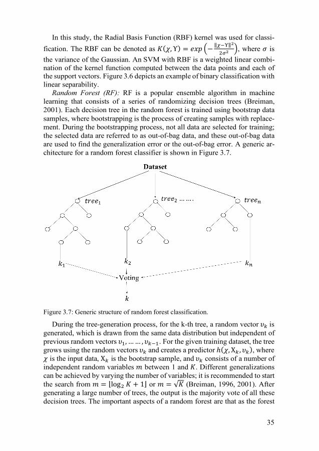
35
In this study, the Radial Basis Function (RBF) kernel was used for classi-fication. The RBF can be denoted as 𝐾(𝜒, Υ) = 𝑒𝑥𝑝 �−‖�p�‖�
I���, where 𝜎 is
the variance of the Gaussian. An SVM with RBF is a weighted linear combi-nation of the kernel function computed between the data points and each of the support vectors. Figure 3.6 depicts an example of binary classification with linear separability.
Random Forest (RF): RF is a popular ensemble algorithm in machine learning that consists of a series of randomizing decision trees (Breiman, 2001). Each decision tree in the random forest is trained using bootstrap data samples, where bootstrapping is the process of creating samples with replace-ment. During the bootstrapping process, not all data are selected for training; the selected data are referred to as out-of-bag data, and these out-of-bag data are used to find the generalization error or the out-of-bag error. A generic ar-chitecture for a random forest classifier is shown in Figure 3.7.
Figure 3.7: Generic structure of random forest classification.
During the tree-generation process, for the k-th tree, a random vector 𝜐his generated, which is drawn from the same data distribution but independent of previous random vectors 𝜐B, …… , 𝜐hpB. For the given training dataset, the tree grows using the random vectors 𝜐h and creates a predictor ℎ(𝜒, Χh, 𝜐h), where 𝜒 is the input data, Χh is the bootstrap sample, and 𝜐h consists of a number of independent random variables 𝑚 between 1 and 𝐾. Different generalizations can be achieved by varying the number of variables; it is recommended to start the search from 𝑚 = ⌊logI 𝐾 + 1⌋ or 𝑚 = √𝐾 (Breiman, 1996, 2001). After generating a large number of trees, the output is the majority vote of all these decision trees. The important aspects of a random forest are that as the forest
59
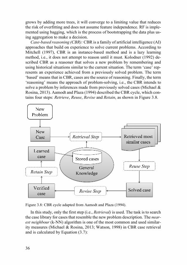
36
grows by adding more trees, it will converge to a limiting value that reduces the risk of overfitting and does not assume feature independence. RF is imple-mented using bagging, which is the process of bootstrapping the data plus us-ing aggregation to make a decision.
Case-based reasoning (CBR): CBR is a family of artificial intelligence (AI) approaches that build on experience to solve current problems. According to Mitchell (1997), CBR is an instance-based method and is a lazy learning method, i.e., it does not attempt to reason until it must. Kolodner (1992) de-scribed CBR as a reasoner that solves a new problem by remembering and using historical situations similar to the current situation. The term ‘case’ rep-resents an experience achieved from a previously solved problem. The term ‘based’ means that in CBR, cases are the source of reasoning. Finally, the term ‘reasoning’ means the approach of problem-solving, i.e., the CBR intends to solve a problem by inferences made from previously solved cases (Michael & Rosina, 2013). Aamodt and Plaza (1994) described the CBR cycle, which con-tains four steps: Retrieve, Reuse, Revise and Retain, as shown in Figure 3.8.
Figure 3.8: CBR cycle adapted from Aamodt and Plaza (1994).
In this study, only the first step (i.e., Retrieval) is used. The task is to search the case library for cases that resemble the new problem description. The near-est neighbour (k-NN) algorithm is one of the most common and used similar-ity measures (Michael & Rosina, 2013; Watson, 1998) in CBR case retrieval and is calculated by Equation (3.7):
60

37
𝑆𝑖𝑚𝑖𝑙𝑎𝑟𝑖𝑡𝑦(𝑇, 𝑆) =j𝑤q
C
qtB
∗ 𝑓(𝑇q, 𝑆q) (3.7)
where 𝑇 is the target case, 𝑆is the source case, 𝑛 is the number of features in each case, 𝑖 is the index of individual features, 𝑓 is a similarity function, and 𝑤 is the weighting parameter of the 𝑖-th feature.
Hierarchical clustering: Clustering is an unsupervised method that groups a set of data objects into clusters such that the data within a cluster have high similarity and are less dissimilar to the data in other clusters. Clustering is used in PAPER II to group the artifactual and non-artifactual components extracted from EEG signals. According to Jain, et al. (1999), clustering organ-izes a collection of patterns or feature vectors into clusters based on similarity measures applied to unlabelled data. Similarities are quantified based on the distance measures of the features or attribute values that describe the objects (Han, 2005). Hierarchical clustering is one of the clustering algorithms that group data objects into a hierarchy or “tree” of clusters, also known as a den-drogram. Based on the hierarchical decomposition approach, hierarchical clustering can be classified as either agglomerative (bottom-up) or divisive (top-down). In the agglomerative approach, each object starts by forming a separate group; then, the groups or objects that are close to one another are iteratively merged. This process continues until all the groups have been merged into one, or until a termination condition becomes true. In the divisive approach, the clustering process starts by considering all the objects as being in the same cluster. During a successive iteration process, clusters are subdi-vided into smaller clusters until each object is in a single cluster or a termina-tion condition applies (Han, 2005). Moreover, hierarchical-clustering algo-rithms can be distance-based or density- and continuity-based.
Figure 3.9: (a) Points falling in three clusters, (b) The dendrogram representation (Jain, et al., 1999).
61

38
Figure 3.9 depicts an example of clustering and a dendrogram representa-tion of the clusters. The tree is not a single set of clusters but rather a multilevel hierarchy, where clusters at one level are joined to clusters at the next level (G. Chen, et al., 2002). Hierarchical clustering can be variations of single link, complete link, and minimum variance algorithms. Among these three variants, the single link and complete link methods are the most popular. In the single link algorithms, patterns are drawn from two clusters, and the minimum of the distances between all pairs is the distance between two clusters. In contrast, in the complete link, the maximum of all pairwise distances is the distance be-tween two clusters. The complete link algorithm produces more compact clus-ters than does the single link algorithm. Moreover, in many practical applica-tions, a complete link algorithm produces more useful hierarchies than does a single link algorithm (Han, 2005). In PAPER II, the furthest distance algo-rithm (i.e., a complete link measured using the Euclidean distance function) is applied. An inconsistency coefficient threshold of 1.1 was used to group the data into an unknown number of clusters.
3.4.4 Phase 4: Comparison Performances of the Classifiers The results obtained in the previous phase were used to compare the perfor-mances among the tested classifiers. In addition, comparisons of the classifi-cation performances considering the data sources were conducted. These in-clude features from both individual data and multiple data sources, features from individual signals, and features based on data fusion, both with and with-out contextual features, and the performances with different feature subsets.
62

39
Chapter 4
Experiments and Results This chapter describes the data analysis and results obtained following the methodology presented in the Chapter 3 to the datasets.
The experimental work and the achieved results from EEG artifact handling, driver sleepiness classification, cognitive load classification and stress classi-fication are presented in this chapter. Results from additional experiments that were not included in PAPER I-V are also included in this chapter.
4.1 EEG Artifact Handling The Automated aRTifact handling in EEG (ARTE) algorithm is a data-driven approach that does not rely on additional reference signals or manually de-fined thresholds. ARTE combines several techniques to identify and reduce EEG artifacts, including the wavelet transform, independent component anal-ysis (ICA), and hierarchical clustering. The quality of the cleaned EEG signals was assessed both quantitatively and subjectively by an expert [PAPER II]. The performance of ARTE was also compared to that of a state-of-the-art method called FORCe. The so-called signal quality index (SQI) (Daly, et al., 2012), the relative error (RE) (Malik M. Naeem Mannan, et al., 2016), the normalized root mean square error (NRMSE), and the mean absolute error (MAE) (Betta, et al., 2013) were used in the quantitative evaluation. Three separate analyses of variance (ANOVAs) were used to compare ARTE and FORCe. For the expert’s evaluation, 210 samples of 60-second segments (70 segments of raw EEG, 70 segments cleaned using ARTE, and 70 segments cleaned with FORCe) were chosen for manual evaluation. The expert scored five different parameters for each segment based on visual observation; see Table 4.1. Differences between expert ratings for the raw data and the two algorithms were tested using five separate Kruskal-Wallis tests.
The score of the 1st parameter represents the number of channels affected by artifacts; for the 2nd parameter and 4th parameter, a score of 0 indicates that there are no or minor signs of artifacts in the EEG, whereas a score of 10 indicates heavy contamination of artifacts within the channel(s). The scores of
63
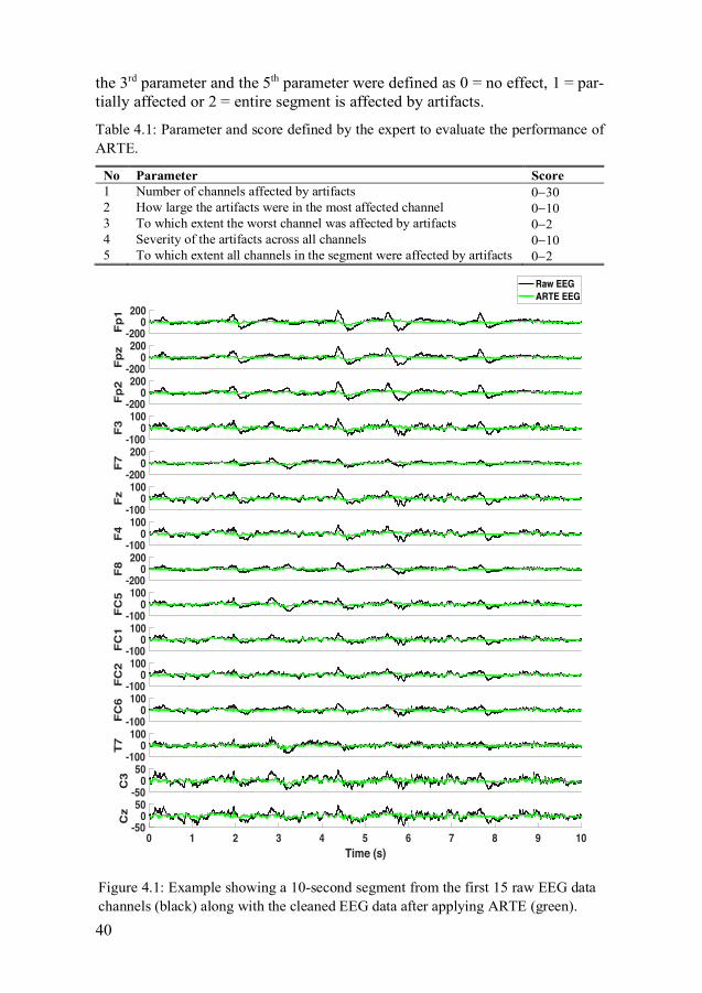
40
the 3rd parameter and the 5th parameter were defined as 0 = no effect, 1 = par-tially affected or 2 = entire segment is affected by artifacts.
Table 4.1: Parameter and score defined by the expert to evaluate the performance of ARTE.
No Parameter Score 1 Number of channels affected by artifacts 0-30 2 How large the artifacts were in the most affected channel 0-10 3 To which extent the worst channel was affected by artifacts 0-2 4 Severity of the artifacts across all channels 0-10 5 To which extent all channels in the segment were affected by artifacts 0-2
-2000
200
Fp
1
-2000
200
Fp
z
-2000
200
Fp
2
-1000
100
F3
-2000
200
F7
-1000
100
Fz
-1000
100
F4
-2000
200
F8
-1000
100
FC
5
-1000
100
FC
1
-1000
100
FC
2
-1000
100
FC
6
-1000
100
T7
-500
50
C3
0 1 2 3 4 5 6 7 8 9 10Time (s)
-500
50
Cz
Raw EEGARTE EEG
Figure 4.1: Example showing a 10-second segment from the first 15 raw EEG data channels (black) along with the cleaned EEG data after applying ARTE (green).
64

41
Figure 4.1 and Figure 4.2 show examples of EEG artifact handling by ARTE when applied to 10 seconds of typical EEG data recorded while driv-ing. As show, frontal EEG channels were affected by ocular artifacts, and some muscle artifacts or noise occurred in the parietal and central EEG chan-nels. Both types of artifacts were removed or reduced after applying ARTE.
Figure 4.2: The remaining 15 channels from Figure 4.1.
The 30 EEG channels were grouped into four regions (frontal, temporal, central, and rear regions) before calculating SQI, RE, NRMSE, and MAE. Significant differences in mean SQI were found for the factor Algorithm
-500
50
C4
-500
50
T8
-1000
100
CP
5
-500
50
CP
1
-500
50
CP
2
-500
50
CP
6
-1000
100
P7
-500
50
P3
-500
50
Pz
-500
50
P4
-500
50
P8
-500
50
PO
z
-500
50
O1
-500
50
Oz
0 1 2 3 4 5 6 7 8 9 10Time (s)
-500
50
O2
Raw EEGARTE EEG
65

42
(𝐹(I,§B��) = 1766.79, 𝑝 < 0.001). The main difference was found between raw and cleaned EEG, but it was also found that the FORCe algorithm pro-vided lower SQI values than those provided by ARTE. Similar results were obtained for the standard deviation of SQI values (𝐹(I,§B��) = 1871.37, 𝑝 <0.001). No significant differences were found between ARTE and FORCe in terms of NRMSE (𝐹(B,Bu�I) = 0.19, 𝑝 = 0.66) and MAE (𝐹(B,Bu�I) =1.78, 𝑝 = 0.18). A significant difference was found for the confounding fac-tor Region (NRMSE:𝐹(�,Bu�I)t63.81, 𝑝 < 0.001 and MAE:𝐹(�,Bu�I)t38.39, 𝑝 < 0.001) and Frequency band (NRMSE:𝐹(�,Bu�I)t285.4, 𝑝 < 0.001 and MAE:𝐹(�,Bu�I)t861.24, 𝑝 <0.001). Statistical analyses of the subjective expert ratings showed a signifi-cant difference for the factor Algorithm (𝐹(I,Iu§) = 18.36, 𝑝 < 0.001) for the 1st parameter; however, there was no difference between ARTE and FORCe, only between raw and cleaned EEG data. Similar results were found for the 2nd parameter (𝜒I(2, 𝑛 = 70) = 79.01, 𝑝 < 0.001) and for the 4th parameter (𝜒I(2, 𝑛 = 70) = 48.97, 𝑝 < 0.001). Furthermore, the expert evaluation showed that 83% of the raw EEG data were fully affected by artifacts, com-pared to 37% after applying FORCe and 30% after applying ARTE. The cor-responding percentages for fully affected segments on all channels were 2%, 63% and 69% for raw, FORCe and ARTE, respectively.
Accuracy Sensitivity Specificity0
5
10
85
90
95
100RawARTEFORCe
Figure 4.3: Achieved accuracy, sensitivity, and specificity of sleepiness binary classifi-cation using SVM.
66

43
The importance of artifact handling in driver monitoring applications was demonstrated by adding artifact handling as a pre-processing step in driver sleepiness classification [PAPER II]. The sleepiness level was defined as alert or sleepy based on subjective self-ratings (alert: KSS≤5, sleepy: KSS≥8). The binary classification was carried out using an SVM with a Gaussian ker-nel, where the parameters C and gamma were set within the range [0.001, 10]. The dataset was randomly divided into a training dataset containing 70% of the data and a test dataset with the remaining 30% of the data. Three separate SVM classifiers were generated, one for the raw EEG, one after applying ARTE and one after applying FORCe. Figure 4.3 shows the sleepiness classi-fication results in terms of accuracy, sensitivity, and specificity on the test dataset. Compared to sleepiness classification using raw EEG, classification performance improved by 5% after applying ARTE and by 2% after applying FORCe.
In summary, the quantitative measures showed that ARTE is comparable to FORCe. The expert evaluation showed that ARTE performed better than FORCe in terms of overall artifact handling but that FORCe could remove artifacts better from some of the individual channels. Most importantly, ARTE resulted in a 5% improvement in classification performance in an actual driver monitoring application. This result can be compared to a 2% improvement for FORCe. It is also worth mentioning that ARTE does not remove any inde-pendent components and instead performs artifact handling by wavelet de-noising and despiking.
4.2 Sleepiness Classification The objective of sleepiness classification was to exploit physiological (EEG and EOG) as well as contextual data (extracted from scenario design), and KSS was the target value in a supervised machine learning configuration [PA-PER III]. The time resolution of one KSS rating was once every fifth minute, but for feature extraction, each five-minute segment was split into five one-minute segments. This strategy provided not only a larger dataset but also re-duced the effects of corrective driving manoeuvres and sensitivity to small variations since actions taken by a driver last a few seconds (D. Sandberg, et al., 2011).
Table 4.2: List of features extracted from the data.
Signal Extracted Features
EEG Frequency bands: δ(<4 Hz), θ(4-7 Hz), α(8-12 Hz), β(12-30 Hz), γ (31-50 Hz), and the ratio (𝜃 + 𝛼)/𝛽, 𝛼/𝛽, (𝜃 + 𝛼)/(𝛼 + 𝛽), and 𝜃/𝛽
EOG Blink durations and PERCLOS Contextual Sleep/wake predictor (SWP), road condition in the scenario i.e., rural/urban
road, and light condition in the scenario i.e., daylight/darkness
67

44
Features extracted from the EEG, EOG, contextual data are listed in Table 4.2. Details of the feature extraction process can be found in PAPER III. In total, features were obtained from 9310 one-minute segments out of 312 drives, and the feature vector consisted of 275 features: 270 features from 30 channels EEG, 2 features from EOG and 3 contextual features. The overall classification task was divided into two phases: first feature selection and then classifier design. The dataset split into training and test datasets, with 70% of the observations in the training set and the remaining 30% of the observations in the test dataset.
Three sleepiness levels were defined based on the KSS: alert (KSS 1 – 5), somewhat sleepy (6 ≤ KSS ≤ 7) and sleepy (KSS ≥ 8). The motivation for creating sleepiness levels is based on the fact that KSS ratings 8 and 9 are associated with severe signs of physiological sleepiness and increase the fre-quency of lane-departure incidents (Reyner & Horne, 1998). Classifiers were designed in four ways:
• Multiclass classification — considering all three groups • Binary class with alert and sleepy groups — excluding data of some-
what sleepy group • Binary class with SVM prediction-based — redistribution of observa-
tions from the somewhat sleepy group into the alert and sleepy groups, and
• Binary class with fuzzy centroid-based —redistribution of the obser-vations from the somewhat sleepy group into the alert and sleepy groups.
The creation of binary classifications was motivated by the fact that it might be challenging to self-rate this “in-between” state (D. Sandberg, et al., 2011). Four classifiers, namely, KNN, SVM, CBR and random forest (RF), were sep-arately trained using the training dataset. In addition, the first binary class, i.e., excluding data for the somewhat sleepy group because of the crisp division between the alert and sleepy groups, allowed for better discrimination. How-ever, in reality, all data need to be considered; therefore, two semi-supervised approaches were considered to redistribute the data of the somewhat sleepy group into the alert and sleepy groups.
4.2.1 Feature Selection A large number of features were obtained from the EEG signals, many of which were recorded from neighbouring electrodes. Hence, we expected that these features might overlap and contain irrelevant or duplicate features. Re-ducing the size of the feature vector could improve the performance of the classifier and could be beneficial for understanding the data and gaining knowledge about the data generation, i.e., sleepiness. Seven feature selection algorithms (BSS/WSS, SFFS, mRMR, BIRS, Relief, LASSO and NCA; see section 3.4.2) were applied using the training dataset to obtain a subset of
68

45
features that were later used in the classifier design phase. Furthermore, the training dataset was divided into two sets, with 80% for feature selection and 20% of the training data as a validation set.
SWP was the top-ranked feature among five of the seven feature selection algorithms, namely, BSS/WSS, SFFS, mRMR, Relief, and BIRS. NCA se-lected SWP as the second-ranked feature. Light condition was ranked the highest by the NCA, but its rank was lower among the other algorithms. Light condition was ranked 43rd by BSS/WSS, 4th by SFFS and BIRS, and 28th by mRMR. Road condition was ranked much lower than the previous two con-textual features; road condition was ranked 47th by BSS/WSS and 3rd by NCA, and the rest of the algorithms did not include road condition in the feature subset. The only exception was LASSO, which did not show sparsity for the contextual features (LASSO results for the three contextual features). Features selected by BSS/WSS as well as by mRMR and Relief essentially consisted of clusters or groups containing similar information. For example, both BSS/WSS and Relief included eye closure-related EOG features and (𝜃 + 𝛼)/(𝛼 + 𝛽) from ten different frontal electrode sites, Fp1, Fp2, Fpz, F3, F4, F7, F8, FC1, FC6, and Fz. Similarly, mRMR included (𝜃 + 𝛼)/(𝛼 + 𝛽) from four different frontal electrode sites, Fp1, Fp2, Fpz, and F3. SFFS also selected (𝜃 + 𝛼)/(𝛼 + 𝛽) but only from one electrode site, i.e., F4 electrode (for details, see PAPER III).
All of these algorithms were separately wrapped with an SVM to evaluate the optimal feature subset using different threshold values. For example, in
Table 4.3, the optimal feature subset from BSS/WSS was obtained for the threshold value of 0.08. The results showed close similarity in classification accuracy, sensitivity, and specificity when using all 275 features (threshold value 0), when using 57 features (threshold value 0.08) and when using 180 features (threshold value 0.02). However, decreased classification accuracy, sensitivity and specificity were observed when fewer than 57 features were selected by BSS/WSS [PAPER III].
Table 4.3 shows the performance of binary classification (alert versus sleepy excluding the somewhat sleepy group) on the validation dataset for each of the algorithms with the number of features in each subset. In PAPER III, the performance of the BSS/WSS, SFFS, and mRMR algorithms was ex-amined. Additional analyses of the feature selection performance of the Re-lief, NCA, BIRS and LASSO algorithms were then performed to explore whether other filter, wrapper or embedded methods could identify better fea-ture subsets that improved the classification performance. NCA showed better results than those of SFFS and mRMR; the number of features selected by NCA was much greater than that selected by SFFS and mRMR, and a similar subset of features matched those selected by BSS/WSS. Compared to the SFFS and mRMR methods, BIRS, Relief, and LASSO did not show any im-provement with respect to the number of features, classification performance or similarity in the subset of selected features.
69

46
Table 4.3: Evaluation of the feature selection algorithms on selected subset of features.
BSS/WSS SFFS mRMR BIRS Relief LASSO NCA #features 57 10 30 16 46 86 60 Sensitivity 0.96 0.92 0.86 0.75 0.80 0.69 0.94 Specificity 0.92 0.91 0.85 0.89 0.90 0.87 0.87 Accuracy 0.94 0.86 0.90 0.72 0.77 0.67 0.91
One of the objectives of feature selection was to investigate the importance of contextual features in classifying sleepiness. Hence, comparisons were made between classifications with and without contextual features. In this ex-periment, feature subsets were obtained from BSS/WSS with a threshold of 0.02, which provided the best classification performance with the validation set [PAPER III], followed by multiclass and binary classification using SVM. The best classification performance is presented in Table 4.4; notably, perfor-mance increased when contextual features were included, particularly the SWP feature.
Table 4.4: Comparison of SVM evaluation of BSS/WSS feature selection. Results show best performance when contextual features were included and excluded. Here, In = including contextual features and Out = excluding contextual features; SEN = sensitivity, SPE = specificity and ACC = accuracy.
Criteria Multiclass Binary classification excluding some-what sleepy
Binary classification SVM predic-tion-based
Binary classification Fuzzy centroid-based
In Out In Out In Out In Out SEN 0.80 0.76 0.95 0.94 0.93 0.88 0.94 0.92 SPE 0.85 0.80 0.94 0.91 0.92 0.91 0.94 0.91 ACC 0.92 0.87 0.95 0.93 0.93 0.85 0.95 0.92
4.2.2 Classification Scheme and Evaluation of Classifiers Evaluation of each classifier for both multiclass and binary classification was performed using (a) 10-fold cross-validation and (b) leave-one-out (LOO) val-idation with one participant left out (except the binary classification excluding data of somewhat sleepy group) and (c) leave-one-out (LOO) validation with one KSS left out. Ten-fold cross-validation was used when training the models on the training dataset containing a subset of features selected using the BSS/WSS method.
Multiclass classification using 10-fold cross-validation on the training da-taset showed 78% accuracy for KNN, 80% accuracy for SVM, 77% accuracy for RF, and 33% accuracy for CBR. Figure 4.4 shows the prediction perfor-mance with respect to accuracy, sensitivity and specificity using the test da-taset; in particular, a decrease in performance was observed using LOO
70
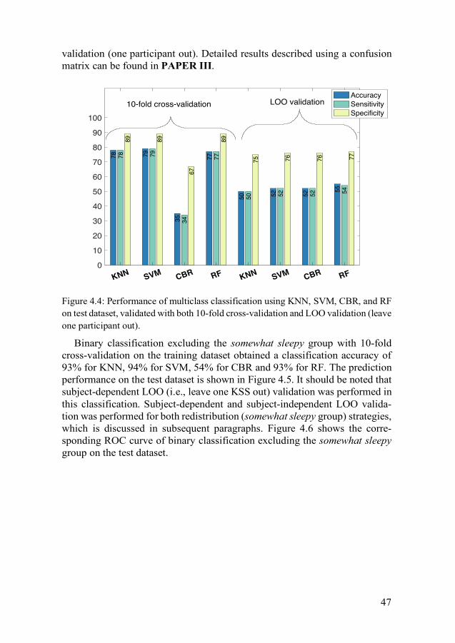
47
validation (one participant out). Detailed results described using a confusion matrix can be found in PAPER III.
Figure 4.4: Performance of multiclass classification using KNN, SVM, CBR, and RF on test dataset, validated with both 10-fold cross-validation and LOO validation (leave one participant out).
Binary classification excluding the somewhat sleepy group with 10-fold cross-validation on the training dataset obtained a classification accuracy of 93% for KNN, 94% for SVM, 54% for CBR and 93% for RF. The prediction performance on the test dataset is shown in Figure 4.5. It should be noted that subject-dependent LOO (i.e., leave one KSS out) validation was performed in this classification. Subject-dependent and subject-independent LOO valida-tion was performed for both redistribution (somewhat sleepy group) strategies, which is discussed in subsequent paragraphs. Figure 4.6 shows the corre-sponding ROC curve of binary classification excluding the somewhat sleepy group on the test dataset.
KNN SVM CBR RF KNN SVM CBR RF
78 7889
79 7989
35 3467
77 7789
50 5075
52 5276
52 5276
55 5477
0
10
20
30
40
50
60
70
80
90
100
AccuracySensitivitySpecificity
LOO validation10-fold cross-validation
71

48
Figure 4.5: Performance of binary classification, excluding somewhat sleepy group using KNN, SVM, CBR, and RF on test dataset, validated with both 10-fold cross-validation and LOO validation (leave one KSS out).
Figure 4.6: ROC curves of KNN, SVM and CBR and RF classifiers on the test dataset, where the models were trained using 10-fold cross-validation and LOO (leave one KSS out).
0 0.1 0.2 0.3 0.4 0.5 0.6 0.7 0.8 0.9 1False positive rate
0
0.1
0.2
0.3
0.4
0.5
0.6
0.7
0.8
0.9
1
True
pos
itive
rate
KNN 10-fold, AUC 0.98SVM 10-fold, AUC 0.98CBR 10-fold, AUC 0.55RF 10-fold, AUC 0.98KNN LOO, AUC 0.93SVM LOO, AUC 0.93CBR LOO, AUC 0.93RF LOO, AUC 0.93
KNN SVM CBR RF KNN SVM CBR RF
93 92 94 94 95 92
4954
39
93 94 92
88 87 89 89 90 88 91 91 92
88 88 89
0
10
20
30
40
50
60
70
80
90
100
AccuracySensitivitySpecificity
LOO validation10-fold cross-validation
72

49
Binary classification using the training dataset and SVM prediction-based redistribution of the somewhat sleepy group achieved classification accuracies of 10-fold cross-validation of 92% for KNN, 94% for SVM, 50% for CBR, and 91% for RF. Additionally, binary classification using the training dataset and fuzzy centroid-based redistribution of the somewhat sleepy group achieved classification accuracies of 10-fold cross-validation of 88% for KNN, 89% for SVM, 54% for CBR, and 88% for RF. The prediction perfor-mances of the classifiers for both binary classifications are presented in Table 4.5, and details can be found in PAPER III. Figure 4.7 shows the correspond-ing ROC curve of both binary classifications on the test dataset.
Table 4.5: Performance summary of the classifiers for binary classification, 10-fold cross-validation on the test dataset.
Criteria SVM predicted redistribution of the “Somewhat Sleepy” Group
Fuzzy centroid redistribution of the “Somewhat Sleepy” Group
KNN SVM CBR RF KNN SVM CBR RF TP 1400 1389 823 1379 1549 1533 1281 1529 FP 91 102 668 112 119 135 387 139 FN 138 82 705 143 217 177 859 206 TN 1164 1220 597 1159 908 948 266 919 Sensitivity 0.91 0.94 0.54 0.91 0.88 0.90 0.60 0.87 Specificity 0.93 0.92 0.47 0.91 0.88 0.88 0.41 0.88 Accuracy 0.92 0.93 0.51 0.91 0.88 0.89 0.55 0.88
0 0.1 0.2 0.3 0.4 0.5 0.6 0.7 0.8 0.9 1False positive rate
0
0.1
0.2
0.3
0.4
0.5
0.6
0.7
0.8
0.9
1
True
pos
itive
rate
KNN using SVM predicted redistribution, AUC 0.97SVM using SVM predicted redistribution, AUC 0.98CBR using SVM predicted redistribution, AUC 0.53RF using SVM predicted redistribution, AUC 0.97KNN using fuzzy centroid redistribution, AUC 0.95SVM using fuzzy centroid redistribution, AUC 0.95CBR using fuzzy centroid redistribution, AUC 0.55RF using fuzzy centroid redistribution, AUC 0.94
Figure 4.7: ROC curves for KNN, SVM, CBR, and RF classifiers on the test dataset, where the models were trained using 10-fold cross-validation.
73

50
Similarly, prediction performance was measured by evaluating the classi-fiers using LOO validation with one participant left out.
Table 4.6 shows the prediction performance of the four classifiers after SVM prediction-based redistribution of the somewhat sleepy group and the prediction performance of the four classifiers after fuzzy centroid-based redis-tribution of the somewhat sleepy group. Details can be found in PAPER III. Figure 4.8 shows the corresponding ROC curve of binary classification for SVM-based and fuzzy centroid-based redistribution of the somewhat sleepy group on the test dataset.
Table 4.6: Performance summary of the classifiers for binary classification, LOO val-idation (leave one participant out) on the test dataset.
Criteria SVM predicted redistribution of “Somewhat Sleepy” Group
Fuzzy centroid redistribution of “Somewhat Sleepy” Group
KNN SVM CBR RF KNN SVM CBR RF TP 2163 1878 2076 2073 4020 3667 4373 3855 FP 1337 1622 1424 1427 1420 1773 1067 1585 FN 1524 1063 1021 1157 1585 1067 1198 1244 TN 4286 4747 4789 4653 2285 2803 2672 2626 Sensitivity 0.59 0.64 0.67 0.64 0.72 0.77 0.78 0.76 Specificity 0.76 0.75 0.77 0.77 0.62 0.61 0.71 0.62 Accuracy 0.69 0.71 0.74 0.72 0.74 0.69 0.76 0.70
0 0.1 0.2 0.3 0.4 0.5 0.6 0.7 0.8 0.9 1False positive rate
0
0.1
0.2
0.3
0.4
0.5
0.6
0.7
0.8
0.9
1
True
pos
itive
rate
KNN using SVM predicted redistribution, AUC 0.74SVM using SVM predicted redistribution, AUC 0.74CBR using SVM predicted redistribution, AUC 0.62RF using SVM predicted redistribution, AUC 0.77KNN using fuzzy centroid redistribution, AUC 0.71SVM using fuzzy centroid redistribution, AUC 0.75CBR using fuzzy centroid redistribution, AUC 0.73RF using fuzzy centroid redistribution, AUC 0.76
Figure 4.8: ROC curves for KNN, SVM, CBR, and RF classifiers, where models were evaluated using leave-one-out validation with leave one participant out.
74

51
Finally, subject-dependent LOO evaluation with one KSS left out showed improved classification performance by including individuals’ observation in the training dataset. As shown in Table 4.7 (details in PAPER III), the clas-sification accuracy increased by up to 10% in subject-dependent classification compared to subject-independent classification.
Table 4.7: Performance summary of the classifiers for binary classification consider-ing participant dependent observations, i.e., LOO with leave one KSS out.
Criteria SVM predicted redistribution of “Somewhat Sleepy” Group
Fuzzy centroid redistribution of “Somewhat Sleepy” Group
KNN SVM CBR RF KNN SVM CBR RF Sensitivity 0.73 0.76 0.80 0.77 0.79 0.82 0.85 0.81 Specificity 0.84 0.84 0.84 0.86 0.69 0.70 0.81 0.71
Accuracy 0.80 0.81 0.82 0.83 0.75 0.77 0.83 0.77
In summary, the feature selection process showed that it might be beneficial to consider certain overlapping features when addressing noisy and imbalance data as with BSS/WSS. Second, contextual features, particularly SWP, were found to be the most influential for improving classification performance. Adding contextual infor-mation improved multiclass classification accuracy by 4% and by 5%, as indicated by the binary classification results. Third, the effect of individual differences was also investigated, showing a 10% increase in accuracy when data from the individual being evaluated were included in the training dataset. Fourth, SVM was the most stable among the four classifiers, demonstrating 79% accuracy for multiclass classification and 93% accuracy for binary classification.
4.3 Cognitive Load Classification The objective of cognitive load classification was to distinguish driving events with cognitive loading tasks from normal driving events. Each scenario had a duration of 60 seconds, and the first 10 seconds of data were discarded because the driver state might not have been stable. Hence, 50 seconds of each scenario recording was used for feature extraction. Various features were obtained from the physiological signals and the vehicular data. Table 4.8 lists features extracted from the signals. For the interested reader, references to each of fea-ture can be found in the chapter detailing the background and related work. In total, the feature matrix consisted of 721 observations, 306 from the baseline or no-task condition, 237 from the 1-back task, and 178 from the 2-back task.
For the cognitive load classification, data from both test series were com-bined, and the binary classification was defined based on whether drivers per-formed a cognitive loading task such that the task was assigned to the task group or baseline group. However, in PAPER IV, data from the first test se-ries were used, and later, cognitive load classification was extended using data from both test series. The baseline group consisted of driving alone or no task
75

52
events, and the task group contained data from both the 1-back and 2-back tasks.
Table 4.8: List of features extracted from each of the signal.
Signal Extracted Features
EEG Frequency bands: δ(<4 Hz), θ(4-7 Hz), α(8-12 Hz), β(12-30 Hz), γ (31-50 Hz), and the ratio (𝜃 + 𝛼)/𝛽, 𝛼/𝛽, (𝜃 + 𝛼)/(𝛼 + 𝛽), and 𝜃/𝛽
EOG start position of blink, blink duration calculated from the start position of blink to the end value of blink, lid closure speed, PCV (peak closing velocity), delay of eye lid reopening, duration at 80%, PERCLOS, blink rate, blink count
ECG Time: Mean heart rate (meanHR), standard deviation of heart rate (SDHR), standard deviations of normal to normal RR intervals (SDNN), Root mean square of successive differences between adjacent NN intervals (RMSSD), number of pairs of successive NN intervals which more than 50 ms (NN50), Percentage of NN50 (pNN50) Frequency: Low frequency power (LF) (0.04–0.15Hz), High frequency power (HF) (0.15–0.4Hz), total power, LF/HF ratio Non-linear: Alpha value of detrended fluctuation analysis (dfaAlpha), Sam-ple entropy (SampEn), Approximate entropy (ApEn) and Permutation en-tropy (PeEn)
GSR Time: Number of peaks, the amplitude of the peaks (maxima - minima), du-ration of the rise time of each peak, index of the detected peaks in the GSR signal, Mean value, Standard deviation, first quartile value, third quartile value, slope value between peak and valley. Frequency: Average power of the signal under 1Hz
Respiration Time: Mean value, Standard deviation, kurtosis Frequency: power spectra power between the frequency ranges [0, 0.1], [0.1, 0.2], [0.2, 0.3], [0.3, 0.4], [0.4, 0.7], and [0.7, 1]
Vehicular data
Standard deviation of lateral position, Mean squared error of lateral position Standard deviation of steering wheel angle, steering wheel entropy, steering wheel reversal rate, high frequency component (0.3 Hz), number of zero crossings. Lanex or fraction of lane exit from lane departure. Standard deviation of lateral speed, yaw and yaw rate.
Similarly to the sleepiness classification, the dataset was split into training and test datasets, with 70% of the observations in the training set and the re-maining 30% of the observations in the test dataset. Combining the two test series data and the baseline and task group resulted in an imbalanced dataset (the number of observations in the task group was greater than that in the base-line group); therefore, balanced accuracy (BACC) was estimated to measure the classification performance in addition to the sensitivity, specificity, and accuracy.
76

53
4.3.1 Feature Selection EEG feature selection: The same EEG features described in the sleepiness classification were extracted for cognitive load classification from the EEG signals. The goal was to identify the intra-feature relationships and select the best feature subset. The SFFS algorithm was used in conjunction with SVM to obtain the best feature subset. Five-fold cross-validation was used to eval-uate the SVM classification. The best classification accuracy obtained using SFFS was 66%, with 11 features consisting of 𝜃/𝛽, 𝛼/𝛽, (𝜃 + 𝛼)/𝛽, 𝜃, 𝛽, and 𝛼 features from seven frontal channels, namely, FP1, FP2, F7, F4, FPz, FC2, and FC5. The accuracy, sensitivity, specificity, and classification score (scr) are shown in Figure 4.9. Scr measures the trade-off between sensitivity
and specificity, defined as 2°�±�².³´µ� �.°�±�².³¶´� � (Mekyska, et al., 2015).
Figure 4.9: EEG feature selection using SFFS on the training dataset, validated using 5-fold cross-validation.
Feature selection from combination of all features: Combining features from all data increases the dimensions of the feature matrix. HRV and respi-ration are correlated, and within the vehicular data, redundant information can exist in this fused feature matrix. The feature selection ability of the random forest algorithm was exploited during the cognitive load classification without incorporating any additional feature selection algorithm. The mean-decrease accuracy approach (which directly measures the impact of each feature on the accuracy of the model) was applied to select the best subset of features. In the
0 10 20 30 40 50 60 70 80 90 number of changes in (best) feature set [-]
0
10
20
30
40
50
60
70
80
90
100
acc
, sen
, spe
, scr
[%]
1 2 3 4 5 6 7 8 9 10 11 12
accsenspescr
77

54
mean-decrease accuracy approach, the importance of each feature value is per-muted, and the corresponding decrease in the accuracy of the model is meas-ured. Unimportant features should not have a strong effect on the model accu-racy, but important features should significantly decrease the model accuracy. The features selected from each signal are listed in Table 4.9.
Table 4.9: List of selected features from each of the signal.
Data #Features Features
EEG 11 FP1 –𝛽, FP2 – 𝜃, (𝜃 + 𝛼)/(𝛼 + 𝛽) FP2 – 𝜃, (𝜃 + 𝛼)/(𝛼 + 𝛽) FPz – 𝛽, 𝜃/𝛽, (𝜃 + 𝛼)/𝛽 F4 – 𝜃 F7 – 𝜃 FC2 – 𝜃/𝛽, 𝛼/𝛽
EOG 5 start position of blink, blink duration calculated from the start position of blink to the end value of blink, PERCLOS, blink rate, blink count
ECG 9 Time: SDHR, SDNN, NN50, pNN50 Frequency: LF, HF, LF/HF ratio Non-linear: dfaAlpha, SampEn,
GSR 4 Time: The amplitude of the peaks, duration of the rise time of each peak, Mean value Frequency: Average power of the signal under 1Hz
Respiration 7 Time: Mean value, Standard deviation, kurtosis Frequency: power spectra power between the frequency ranges [0, 0.1], [0.2, 0.3], [0.4, 0.7], and [0.7, 1]
Vehicular data
6 Standard deviation of lateral speed. Standard deviation of lateral speed yaw. Steering wheel entropy, high frequency component (0.3 Hz), and number of zero crossings. Lanex or fraction of lane exit from lane departure.
Scenario 1 Categorial feature to represent HE, CR, and SW scenarios
4.3.2 Classification Scheme and Evaluation of Classifiers This section addresses three types of cognitive load classification:
(1) Classification based on different data sources, i.e., cerebral (EEG), non-cerebral physiological signals (ECG, GSR, and respiration) and vehicular data;
(2) Classification based on the effects of scenarios on cognitive load clas-sification;
(3) Classification based on the combination of features from all signals.
78

55
In all four experiments, KNN, SVM, and RF classifiers were used and eval-uated with 5-fold cross-validation to distinguish between the baseline and task groups. The motivation for these experiments was to investigate whether per-formance improves with feature-level fusion relative to that of the grouped data sources, i.e., cerebral activity, non-cerebral physiological signal and ve-hicular data.
1) Classification based on data sources: In this section addresses three cognitive load classifications: • Classification using features from EEG signals (i.e., cerebral sig-
nals). • Classification using features from ECG, GSR, and respiration sig-
nals (i.e., non-cerebral physiological signals). • Classification using features from vehicular data
Cognitive load classification using EEG signals was carried out using the best subset of features obtained by applying the SFFS algorithm. The training dataset classification accuracy was 58% for KNN and SVM and 61% for RF. Using non-cerebral physiological signals, the classification accuracies for KNN, SVM, and RF were 69%, 71%, and 72%, respectively, on the training dataset with 5-fold cross-validation. Using the features from vehicular data, the classification accuracies were 58% for KNN and SVM and 56% for RF on the training dataset with 5-fold cross-validation. Table 4.10 presents the pre-diction performance results of KNN, SVM and RF on the test dataset for cog-nitive load classification using EEG features; features obtained from ECG, GSR, and respiration signals; and features obtained from vehicular data.
Table 4.10: Classification summary of KNN, SVM, and RF classifiers on test dataset when using EEG feature.
EEG ECG, GSR, respiration
Vehicular
KNN SVM RF KNN SVM RF KNN SVM RF Sensitivity 0.59 0.60 0.67 0.73 0.76 0.75 0.57 0.57 0.58 Specificity 0.47 0.46 0.60 0.72 0.70 0.69 0.43 0.00 0.43 Accuracy 0.57 0.56 0.65 0.73 0.73 0.73 0.55 0.57 0.53 BACC 0.52 0.53 0.62 0.71 0.72 0.72 0.50 0.50 0.51
2) Effects of scenarios on cognitive load classification: Two experiments were conducted to investigate the effect of scenarios on cognitive load classi-fication. The first experiment used data from the first test series (only data from the first test series was available at that time) (see section 3.2), using 270 features obtained from the 30 EEG channels [PAPER IV]. The dataset used in this experiment contained data from 33 participants, who performed the 1-back task and only driving in the test scenario during data collection. The clas-sification task was performed for each scenario and by considering data from
79

56
Figure 4.10: Classification performance of scenario wise binary classification on the test dataset.
a combination of scenarios. Each scenario consisted of 132 observations, and there were 264 observations in the hidden exit and cross scenarios combined; the dataset with all scenarios consisted of 396 observations. Table 4.11 sum-marises the results for each evaluation.
Table 4.11: CBR Classification summary for individual and mixed scenarios.
Scenario Sensitivity Specificity Accuracy Crossing (CR) 0.74 0.70 0.72 Hidden Exit (HE) 0.71 0.86 0.76 Side Wind (SW) 0.70 0.75 0.72 CR+HE 0.76 0.80 0.78 CR+HE+SW 0.72 0.71 0.72
Data from both test series were then used to inspect whether there was any effect of the scenarios on classification performance. Scenario-wise binary classification was carried out using the best selected subset of features pre-sented in Table 4.9 (except the categorical features based on scenarios). Figure 4.10 shows the performance of binary classification for each scenario on the test dataset. For the HE scenario, BAcc(s) were 73%, 65%, and 64% for KNN, SVM, and RF, respectively; in the CR scenario, BAcc(s) were 64% for KNN, 68% for SVM, and 63% for RF; in the SW scenario, BAcc(s) were 72% for KNN, 64% for SVM, and 72% for RF.
00.10.20.30.40.50.60.70.80.9
1
HE Sen
HE Spec
HE Acc
HE BAcc
CR Sen
CR Spec
CR Acc
CR BAcc
SW Sen
SW Spec
SW Acc
SW BAcc
KNNSVMRF
80

57
3) Combination of all features: The results of the cognitive load classifica-tion based on data sources showed similar performance when using features from EEG signals and features from vehicular data. Comparatively, cognitive load classification using features from non-cerebral signals showed better per-formance. Additionally, variation in classification performance was observed in the scenario-wise classification. Hence, the additional categorical feature based on scenarios was included in the best subset of features, as presented in Table 4.9.
Binary classifications were carried out using KNN, SVM, and RF with a combination of features. On the training dataset, classification accuracies of 5-fold cross validation were 67% for KNN, 72% for SVM, and 75% for RF. The prediction performance of KNN, SVM, and RF on the test dataset is pre-sented in Table 4.12.
Table 4.12: Classification summary of KNN, SVM, RF on test dataset.
Criteria KNN SVM RF Task group (P) 126 126 126 Baseline group (N) 89 89 89 TP 116 104 107 FP 10 22 19 FN 47 43 36 TN 42 46 53 Sensitivity 0.71 0.71 0.75 Specificity 0.81 0.68 0.74 Accuracy 0.73 0.70 0.74 BACC 0.70 0.67 0.72
Finally, a multiclass classification was performed with KNN, SVM, and RF to investigate how each class contributed to the classification. On the train-ing dataset using 5-fold cross-validation, the classification accuracies achieved were 53% for KNN, 59% for SVM and RF. Table 4.13 shows the detailed results pertaining to the prediction performance of KNN, SVM, and RF using the test dataset.
Table 4.13: Classification summary of multiclass classification for the KNN, SVM, and RF on test dataset. Where classes are Baseline (BL)= no-task, 1-back and 2-back task. SEN = Sensitivity, SPE = Specificity, PRE = Precision, and ACC = Accuracy.
Criteria KNN SVM RF BL 1-back 2-back BL 1-back 2-back BL 1-back 2-back
TP 60 39 21 66 39 25 70 36 32 FP 32 31 32 26 31 28 22 34 21 FN 37 37 21 38 25 22 37 23 17 TN 86 108 141 85 120 140 86 122 145 SEN 0.62 0.51 0.50 0.63 0.61 0.53 0.65 0.61 0.65 SPE 0.73 0.78 0.82 0.77 0.79 0.83 0.80 0.78 0.87 PRE 0.65 0.56 0.40 0.72 0.56 0.47 0.76 0.51 0.60 BACC 0.68 0.65 0.63 0.70 0.69 0.67 0.73 0.68 0.75
81

58
To summarise, cognitive load classification was carried out considering data sources, scenarios, and feature fusion or a combination of features from all data sources. Feature selection was performed to obtain the best subset of features from the EEG signals using the SFFS algorithm, and the best feature subset was then selected from the combination of all features. The SFFS could find the best subset of features; however, the classification accuracy was poor using only EEG features. Combining features from multivariate data showed a 10% improvement in classification performance compared to using features from EEG signals and a 20% improvement compared to using features vehic-ular data. Cognitive load classification using non-cerebral data showed better performance than any other binary classification method. The multiclass clas-sification results show that classifiers could better classify the no-task events than they could classify 1-back and 2-back task events.
4.4 Stress Classification For the analysis, the dataset containing measurements of wheel loader opera-tor was divided into two groups according to the experiment, i.e., (1) PSP da-taset and (2) training (“adapt”) and testing (“sharp”). An expert, i.e., a clini-cian, annotated the PSP data as either stressed or healthy; however, the expert did not classify the data obtained from the training and testing sessions. Hence, the data obtained from training and testing sessions were annotated as adapt and sharp according to the corresponding sessions. Case-based reasoning was used to classify the stressed and healthy classes and then the adapt and sharp classes. The classification task was performed using the features obtained by applying data fusion, i.e., the MMSE algorithm, and using features extracted from individual signals. To carry out the data analysis, the results from the MMSE analysis were investigated; the evaluation was then performed on the MMSE-CBR classification. Furthermore, decision-level fusion was per-formed using the outcomes from MMSE-CBR classification and the outcomes from CBR classification on individual signals. Table 4.14 presents the list of features extracted from the signals. Majority voting and weighted average similarity approaches were considered for decision-level fusion. Finally, clas-sification performance was evaluated using leave-one-out validation.
Table 4.14: List of features extracted from each of the signal and data fusion.
Data Extracted Features
HRV Time: Mean heart rate, standard deviation of heart rate, standard deviations of normal to normal RR intervals (SDNN), Root mean square of successive differences between adjacent NN intervals (RMSSD), number of pairs of successive NN intervals which more than 50 ms (NN50), Percentage of NN50 (pNN50)
82

59
Frequency: Low frequency power (0.04–0.15Hz), High frequency power (0.15–0.4Hz), total power, LF/HF ratio
Finger Tempera-ture
Time: start value, end value, maximum amplitude, minimum amplitude, slope value between peak and valley, the amplitude of the peaks (maxima - minima)
Respiration Rate
Time: Mean value, Standard deviation, kurtosis Frequency: power spectra power between the frequency ranges [0, 0.1], [0.1, 0.2], [0.2, 0.3], [0.3, 0.4], [0.4, 0.7], and [0.7, 1]
Skin Conduct-ance
Time: Number of peaks, the amplitude of the peaks (maxima - minima), start value, end value, maximum amplitude, minimum amplitude, slope value be-tween peak and valley
Data Fusion MMSE scale 1—10 considering HR, HRV, RR, FT, SC
4.4.1 Evaluation Using the PSP Dataset In this experiment, the MMSE complexity was computed up to a scale factor 10 [PAPER V]. The MMSE algorithm involves a multi-scale analysis of mul-tivariate data, which returns a vector based on the scale factor. The scale factor depends on the number of data points and MMSE estimates consistent for a data length 𝑁 ≥ 300 (Ahmed & Mandic, 2012). As mentioned in Chapter 4, the PSP dataset contained data from 18 participants, among which the expert indicated 7 as healthy and 11 as stressed.
Figure 4.11: MMSE analysis results for the 18 cases, and it can be seen that MMSE varies a lot depending on individuals.
According to Costa, et al. (2005), loss of complexity is noticeable in path-ologic systems. The MMSE analyses of 18 individual cases were estimated,
0 1 2 3 4 5 6 7 8 9 10 11Scale Factor
0.7
0.9
1.1
1.3
1.5
1.7
MM
SE
MMSE Analysis of All CasesCase 1: HealthyCase 2: HealthyCase 3: StressedCase 4: StressedCase 5: StressedCase 6: HealthyCase 7: StressedCase 8: StressedCase 9: HealthyCase 10: StressedCase 11: StressedCase 12: HealthyCase 13: HealthyCase 14: StressedCase 15: StressedCase 16: StressedCase 17: HealthyCase 18: Stressed
83
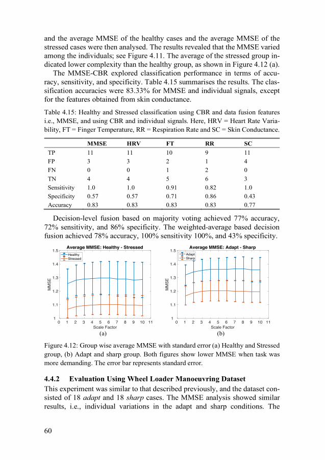
60
and the average MMSE of the healthy cases and the average MMSE of the stressed cases were then analysed. The results revealed that the MMSE varied among the individuals; see Figure 4.11. The average of the stressed group in-dicated lower complexity than the healthy group, as shown in Figure 4.12 (a).
The MMSE-CBR explored classification performance in terms of accu-racy, sensitivity, and specificity. Table 4.15 summarises the results. The clas-sification accuracies were 83.33% for MMSE and individual signals, except for the features obtained from skin conductance.
Table 4.15: Healthy and Stressed classification using CBR and data fusion features i.e., MMSE, and using CBR and individual signals. Here, HRV = Heart Rate Varia-bility, FT = Finger Temperature, RR = Respiration Rate and SC = Skin Conductance.
MMSE HRV FT RR SC TP 11 11 10 9 11 FP 3 3 2 1 4 FN 0 0 1 2 0 TN 4 4 5 6 3 Sensitivity 1.0 1.0 0.91 0.82 1.0 Specificity 0.57 0.57 0.71 0.86 0.43 Accuracy 0.83 0.83 0.83 0.83 0.77
Decision-level fusion based on majority voting achieved 77% accuracy, 72% sensitivity, and 86% specificity. The weighted-average based decision fusion achieved 78% accuracy, 100% sensitivity 100%, and 43% specificity.
(a) (b)
Figure 4.12: Group wise average MMSE with standard error (a) Healthy and Stressed group, (b) Adapt and sharp group. Both figures show lower MMSE when task was more demanding. The error bar represents standard error.
4.4.2 Evaluation Using Wheel Loader Manoeuvring Dataset This experiment was similar to that described previously, and the dataset con-sisted of 18 adapt and 18 sharp cases. The MMSE analysis showed similar results, i.e., individual variations in the adapt and sharp conditions. The
0 1 2 3 4 5 6 7 8 9 10 11Scale Factor
1
1.1
1.2
1.3
1.4
1.5
MM
SE
Average MMSE: Healthy - StressedHealthyStressed
0 1 2 3 4 5 6 7 8 9 10 11Scale Factor
1
1.1
1.2
1.3
1.4
1.5
MM
SE
Average MMSE: Adapt - SharpAdaptSharp
84

61
average MMSE of the adapt condition was higher than that of the sharp con-dition, as shown in Figure 4.12 (b). This discrepancy suggests that sharp or live test driving might be more demanding than adapt or self-training driving. CBR classification was performed to see how well the algorithm could clas-sify the dataset as the recording, i.e., adapt and sharp using MMSE values and features extracted from individual signals. Table 4.16 shows that the best ac-curacy obtained was 83% using the MMSE features rather than the individual signals. The decision fusion considering majority voting achieved a classifi-cation accuracy of 72%, 67% sensitivity and 78% specificity. Finally, decision fusion with the weighted average method achieved 72% classification accu-racy, 89% sensitivity, and 56% specificity.
Table 4.16: Adapt and sharp classification using CBR and data fusion features i.e., MMSE, and using CBR and individual signals. Here, HRV = Heart Rate Variability, FT = Finger Temperature, RR = Respiration Rate and SC = Skin Conductance.
MMSE HRV FT RR SC TP 14 14 16 12 15 FP 1 4 8 5 9 FN 4 4 2 6 3 TN 17 14 10 13 9 Sensitivity 0.78 0.78 0.89 0.67 0.83 Specificity 0.94 0.78 0.56 0.72 0.50 Accuracy 0.83 0.78 0.72 0.69 0.67
In summary, the classification performance of the proposed data fusion method, i.e., the MMSE-CBR approach [PAPER V], is as good as HRV and FT and better than other single source parameters. Single source measure-ments require classification from each source, and the results can also vary between them. The proposed fusion-based approach can be an alternative in cases in which signals are derived from multiple sources and expert classifi-cation is not available for each type of data source. Furthermore, the method described here may yield substantial benefits when applied for decision sup-port in such a domain for monitoring operators and can provide a reasonable means for sensor signal fusion in other health care domains.
85

62
62
86

63
Chapter 5
Summary of the Included Papers This chapter presents a summary of the included papers, author’s contri-butions and the significant findings are also presented here.
This thesis is based on a collection of papers. Papers I and II address RQ1, and the remaining four papers address RQ2, including the sub-questions RQ2.1 and RQ2.2. Paper III presents the work on driver sleepiness classifi-cation, Paper IV presents the work on driver cognitive load classification, and Paper V presents the contribution on driver stress classification.
5.1 Paper I Title: A Review on Machine Learning Algorithms in Handling EEG Artifacts
In the proceeding of the Swedish AI Society (SAIS) Workshop, Stockholm, Sweden
Author(s): Shaibal Barua, Shahina Begum
Author’s contribution: Shaibal Barua is the main author of the paper. He planned and conducted the literature review alone, and wrote the discussion and summary sections in collaboration with the co-author. Objective: The aim of this paper was to review the literature and summarize the state-of-the-art in EEG artifacts handling. Summary: This paper presents a review of machine learning algorithms ap-plied to EEG artifact handling (i.e., artifact identification and removal). Brain wave signals obtained by electroencephalography (EEG) recording are an es-sential aspect of medical, health and brain-computer interface (BCI) research. An EEG is considered nonstationary and non-linear and is usually contami-nated by non-cerebral signals. In EEG signals, the unwanted non-cerebral sig-nals are referred to as artifacts. Due to the nature of EEG signals, noise and artifacts can contaminate the recorded EEG signals, which can lead to severe misinterpretations during EEG signal analysis. In this review, only articles
87

64
reported between 2007 and 2014 were collected and analysed. The collected works were surveyed to identify the sources and types of artifacts, and to col-lect both automated and traditional artifact identification and removal meth-ods. This review also summarizes the machine learning algorithms and ap-proaches used for EEG artifact handling. The survey found that a large number of automatic and semi-automatic methods are available for EEG artifact re-moval, and it provides an analysis of these methods based on their perfor-mances. Results: Independent component analysis (ICA) was found to be the most common method for EEG signal analysis and identifying EEG artifacts; how-ever, ICA requires expert observation to identify artifacts in the EEG signal. Two approaches were identified for artifact identification using ICA: a) threshold based and b) machine learning based. The machine learning ap-proach eases the artifact identification process, where ICA components were classified based on spectral and topographical characteristics. Several ma-chine learning algorithms, such as support vector machines, artificial neural networks, fuzzy inference systems, clustering, k-nearest neighbours, genetic algorithms, etc. The survey suggested focusing on hybrid approaches, i.e., us-ing several machine learning algorithms to identify different types of artifacts in the EEG signals.
5.2 Paper II Title: Automated EEG Artifact Handling with Application in Driver Monitor-ing
IEEE Journal of Biomedical and Health Informatics, 22(5):1350–1361, doi: 10.1109/JBHI.2017.2773999
Author(s): Shaibal Barua, Mobyen Uddin Ahmed, Christer Ahlstrom, Shahina Begum, and Peter Funk
Author’s contribution: Shaibal Barua is the primary author of the paper. Shaibal developed the proposed idea and method and was responsible for writ-ing the manuscript except for the data collection section. Other co-authors contributed by discussing the idea, reviewing and making necessary changes to improve the paper. Objective: The aim of this paper was to develop an EEG artifact handling algorithm for cleaning the EEG signals recorded in an automotive setting. Summary: In this paper, an automated EEG artifact handling method, named ARTE (Automated aRTifacts handling in EEG), was proposed as a pre-pro-cessing step in a driver monitoring application. Automated analyses of
88

65
electroencephalographic (EEG) signals acquired in naturalistic environments are becoming increasingly important in areas such as brain-computer inter-faces and behaviour science. EEG signals acquired in driving were such an application, where ocular and muscle artifacts heavily contaminated the EEG database. The artifacts occurred as a natural consequence of performing sev-eral driving activities such constantly monitoring the environment, which gives rise to eye movements and eye blinks. Muscle artifacts could result be-cause of leaning against the head rest, looking over the shoulder, stretching, slumping, etc. The proposed ARTE comprised signal decomposition, artifact identification, and artifact handling. EEG signals were decomposed using Wavelet transform and Independent Component Analysis (ICA). In the arti-fact identification phase, we used hierarchical clustering based on a large se-lection of features, targeting both physiological and nonbiological artifacts. The artifact handling process consisted of two steps: wavelet despiking and wavelet denoising. To handle artifacts, ARTE was applied to driver sleepiness (see Section 3.1). The algorithm was evaluated both quantitatively (signal quality index, mean square error, relative error and mean absolute error) and quantitatively by a clinical neurophysiologist. ARTE's usefulness was demon-strated as a pre-processing step in driver monitoring, exemplified by driver sleepiness classification. Furthermore, the paper presents a comparison be-tween the performance of ARTE and a state-of-the-art algorithm called FORCe. Results: ARTE and FORCe were comparable regarding their quantitative and expert evaluations. The classification accuracy increased by 5% when using ARTE as a pre-processing step in driver sleepiness classification compared to using raw EEG recordings; however, the classification accuracy increased by 2% when using FORCe in the pre-processing stage. The advantage of ARTE is that it does not rely on additional reference signals or manual thresholds. ARTE is an EEG-data-driven algorithm which makes it well suited for use in dynamic settings where unforeseen and rare artifacts are commonly encoun-tered.
5.3 Paper III Title: Automatic Driver Sleepiness Detection using EEG, EOG and Contex-tual Information
Expert Systems with Applications, 115 (January 2019):121–135, https://doi.org/10.1016/j.eswa.2018.07.054
Author(s): Shaibal Barua, Mobyen Uddin Ahmed, Christer Ahlstrom, Shahina Begum
89

66
Author’s contribution: Shaibal Barua is the main author of the paper. Shai-bal developed the proposed idea and method and was responsible for writing the manuscript except for the data collection section. Other co-authors con-tributed by discussing the idea, reviewing and making necessary changes for the improvement of the paper. Objective: The aim of this paper was investigating if driver sleepiness classi-fication performance improves when taking contextual information into ac-count. Summary: Falling asleep behind the wheel is a common cause of car crashes that has become a major concern for traffic safety because driver sleepiness is a crucial contributing factor to vehicle crashes and traffic injuries. This paper proposed an automated driver sleepiness detection approach. The driver sleep-iness dataset (see Section 3.1) used in this work contained data from 30 par-ticipants who repeatedly drove in a high-fidelity driving simulator, both in alert and in sleep-deprived conditions. The subjective Karolinska sleepiness scale (KSS) was used as the target value. Two sources of data, i.e., physiolog-ical signals consisting of electroencephalography (EEG) and electrooculog-raphy (EOG), and contextual information, including the sleepiness predictor model (SWP) and driving environment condition (road and available light), were used as sleepiness indicators. The sleepiness levels were classified sep-arately using four classifiers: a) k-nearest neighbour, b) support vector ma-chine c) case-based reasoning and d) random forest, and the results were eval-uated and compared. Feature selection, in which various features were ex-tracted from the data mentioned above, was an essential part of this work. We examined the results of the BSS/WSS, SFFS, and mRMR feature selection algorithms. Three sleepiness levels, i.e., alert, somewhat sleepy and sleepy, were considered for multiclass classification, while binary classification was performed considering only alert or sleepy driver states. The evaluation crite-ria used were 10-fold cross-validation and leave-one-out validation. Results: All three feature selection algorithms showed EEG features clustered around the adjacent or symmetric electrode sites. We found that restricting the feature set to a minimal number of EEG features can be error-prone. Among the classifiers, the SVM obtained the most consistent accuracy, sensitivity, and specificity scores. Two critical aspects were found to be of interest: (a) the effect of individual differences (i.e., the classification accuracy increased by up to 10% when data from the individual was included in the training da-taset) and (b) embedding contextual information improved the classification accuracy by 4% in multiclass and 5% in binary classifications.
90

67
5.4 Paper IV Title: Classifying drivers’ cognitive load using EEG signals
Studies in Health Technology and Informatics, 237(pHealth2017):99-106, DOI 10.3233/978-1-61499-761-0-99
Author(s): Shaibal Barua, Mobyen Uddin Ahmed, Shahina Begum
Author’s contribution: Shaibal Barua is the main author of the paper. Shai-bal developed the proposed idea and method and was responsible for writing the manuscript. Other co-authors contributed by discussing the idea, review-ing and suggesting improvements to the paper. Objective: The aim of this paper was to classify drivers’ cognitive load con-sidering in three different driving scenarios using EEG data. Summary: One debatable issue in traffic safety research is that cognitively loading by secondary tasks reduces primary task performance (i.e., driving). An EEG is one available way to measure cognitive load and EEG signal anal-ysis can detect changes in instantaneous load and the effects of cognitively loading secondary tasks. The cognitive load dataset (see Section 3.2) used in this work was acquired to understand the effect of cognitive load on traffic safety and included data collected from 33 subjects in a high-fidelity moving-base driving simulator. The study adopted a version of the n-back task as a cognitively loading secondary task; the drivers drove in three different simu-lated driving scenarios, namely, hidden exit, crossing, and side wind. In this paper, CBR was used to classify a driver’s level of cognitive load using the acquired EEG signals. Both time and frequency domain features were ex-tracted from the EEG signals. Results: The results showed that CBR-based classification achieved approxi-mately 70% accuracy. The best classification accuracy was obtained for the hidden exit scenario, and the lowest accuracy was obtained for the side wind scenario. The assumption was that visual cues in the hidden exit and the car approaching in the crossing scenario might have more influence on the drivers than did the side wind scenario. The combination of time and frequency do-main features reduced the overall accuracy. Combining time and frequency features constructed a high dimensional feature vector, which might lead to the ‘curse-of-dimensionality' trap because the dimensionality of the feature vector was much higher than the total observations.
91
68
5.5 Paper V Title: Classification of physiological signals for wheel loader operators using Multi-scale Entropy analysis and case-based reasoning
Expert Systems with Applications, 41(2):295–305, ISSN 0957-4174 Author(s): Shahina Begum, Shaibal Barua, Reno Filla, Mobyen Uddin Ah-med
Author’s contribution: Shaibal Barua was one of the co-authors of the paper. His contribution includes data processing, features extraction, performing the experiments and developing the prototypal system and its functionality. He also contributed writing in the chapters: Background, Method, Evaluation, Ex-perimental results, and Discussions.
Objective: The aim of this paper was classifying the stressed and healthy group of wheel loader operators using data level fusion. Also, to see if the data level fusion able to classify annotated data based on the study design. Summary: This paper presented a data level fusion for physiological signals using Multivariate Multiscale Entropy Analysis (MMSE). The MMSE algo-rithm supports complexity analysis of multivariate biological recordings by aggregating several sensor measurements, i.e., the inter-beat interval (IBI) and heart rate (HR) from electrocardiograms (ECG), finger temperature (FT), skin conductance (SC) and respiration rate (RR). In the literature, a loss of com-plexity is observed due to the degraded signal information across a broad class of diseases or pathological conditions. In other words, the complexity of healthy systems is greater than the complexity of pathologic systems. In this study, psycho-physiological measurements of wheel loader operators were collected in two phases: the psychophysiological stress profile (PSP) and the operating wheel loader operation, i.e., ‘adapt' (training) and ‘sharp' (real-life driving). The average MMSE of the non-stress condition was higher than the stress condition in the group level, while the MMSE of the adapt condition was higher than the sharp condition. However, there were large variations at the individual level. Therefore, CBR was amended such that CBR looks for similar problem descriptions in the case library built upon past cases and could classify the physiological signals for individuals. Hence, MMSE complexity values were used as features to create the case library for a CBR system. The CBR approach classified unseen cases by retrieving most similar cases from the case library. The proposed approach (i.e., MMSE-CBR) was evaluated us-ing the stress data set (see Section 3.3) obtained from professional wheel loader operators.
92

69
Results: The results showed that for the PSP data the system could classify ‘stressed’ and ‘healthy’ subjects 83.33% correctly compared to an expert’s classification. On the data for the wheel loader operators, the system achieved an accuracy of 83.30% when classifying two different conditions, ‘adapt’ (training) and ‘sharp’ (real-life driving). Hence, the proposed approach, MMSE-CBR, is suitable for use as a classification method and might be of interest for developing systems based on data-level fusion and for working with data collected from several sensor sources.
93

70
70
94

71
Chapter 6
Discussion, Conclusions and Future work This chapter presents the main conclusions of the research work and sum-marize some suggestions for the future work.
The objective of this thesis was multivariate data analysis using machine learning to provide a research support tool for driver state monitoring. The answers to the established research questions are discussed below.
6.1 Discussion on RQs RQ 1: Is it possible to reduce the impact of artifacts and noise in EEG sig-
nals recorded in non-stationary environments such as while driving?
EEG recorded in a non-stationary environment such as a driving vehicle should be affected by un-controlled concomitant stimuli due to excessive mus-cle movement and ocular activities. The use of traditional artifact removal ap-proaches in this context is unreasonable, and new methods should be devel-oped for such applications (Minguillon, et al., 2017). Traditional artifact han-dling methods are often non-automated or semi-automated; in addition, the existing automated methods require reference signals or artifactual template data and manual settings of threshold values for the identification of different artifacts. Furthermore, many of the methods only remove specific artifacts, such as either ocular artifacts or muscle artifacts. Independent component analysis (ICA) is commonly used for multi-channel EEG recording; however, ICA requires manual inspection to identify artifacts, and the recommendation is to use a hybrid approach with one or more machine learning algorithms. The use of a clustering algorithm can be useful for the detection of unforeseen and rare artifacts.
In PAPER II, ARTE (Automated aRTifacts handling in EEG) is proposed as a new algorithm for handling artifacts in EEG signals in a mobile environ-ment. Quantitative evaluation using the measures (SQI, RE, NRMSE, and MAE) provided the time and frequency domain properties of the raw and clean EEG signals. One such property is the large amplitude in the raw EEG influ-enced by eye blinking or distortion in the EEG due to muscle movement. The
95

72
SQI values observed in the raw EEG data were higher than those observed in the clean EEG data, which was also reported by (Daly, et al., 2012; Daly, et al., 2014). The measures RE, NRMSE and MAE also showed significant dif-ferences between the raw and clean EEG data. However, some variations ob-served between the FORCe and ARTE, and for the unforeseen artifacts, arose in the driving situation; thus, it is not easy to obtain an absolute measure of better signals. Some technical issues arise in handling artifacts, such as select-ing the wavelet function for cleaning the artifactual components and running in real time, which are addressed in PAPER II. Because the selection of a wavelet function depends on the nature of the artifacts and the application do-main of EEG signals (Al-Qazzaz, et al., 2015; Khatun, et al., 2016; Khatwani & Tiwari, 2014; Mamun, et al., 2013), several wavelets are investigated when designing ARTE, and the most suitable function appears to be Symlet 4. Sym-let 4 is composed of symmetrical wavelets, and the shape of Symlet 4 mimics the spikes caused by ocular and cardiac artifacts. The average execution time of a 2-second segment is approximately 1.8 seconds with the initial 2-second delay caused by the window function in the pre-processing phase. The time resolution of driver sleepiness detection is typically 1 minute, which is suffi-cient for the required time interval. Finally, the 5% improvement in classifi-cation accuracy, sensitivity, and specificity after artifacts are addressed using ARTE compared to the sleepiness classification using the raw EEG signals confirms the concept that EEG artifact handling is required before EEG signal analysis, particularly for EEG recorded in a dynamic environment such as a driving vehicle.
RQ 2: Can multivariate multimodal data be used to classify driver sleepi-
ness, cognitive load, and stress?
To address this question, different approaches such as data-level fusion, feature-level fusion, decision-level fusion, incorporating contextual data into feature vectors, and classification comparison considering a single source and multi-source features have been investigated in this thesis.
The importance of contextual information for sleepiness classification is pre-sented in PAPER III, in which the classification accuracy improved by 4% in multiclass classification and by 5% in binary classification. The improve-ment may appear small; however, the performance can be further improved with advanced sampling methods for imbalanced datasets. Moreover, real-world driving is much more complex than simulated driving. Driving states are often subjective experiences, in which many other contextual data can play a vital role. The work described in this thesis indicates further investigation in this area, as suggested in (Fu, et al., 2016; McDonald, et al., 2018). For exam-ple, in PAPER III, road conditions are used in sleepiness classification, and in Chapter 4 (Section 4.3), scenarios (which also represent road conditions) are considered contextual features. However, the problem with this approach
96

73
is that these features only represent a portion of the driving conditions, whereas probabilistic measures, as presented in (Fu, et al., 2016) are not gen-eralised but subject- and environment-dependent; nevertheless, no significant improvement in ROC and AUC was found by McDonald, et al. (2018). The use of SWP as features may appear unreasonable. Modern vehicles are already equipped with a wireless network and can synchronise with smart devices. In the future, personalised information such as sleeping hours and waking time can be integrated with smart devices and synchronised with vehicles. Mårtens-son, et al. (2018) showed that SWP estimation considering time awake and time of day could provide quite good results; the proposed model assumes that a person wakes at approximately 7 am. The limitation of SWP is that it func-tions with group mean data, and for different sleep patterns (e.g., those of shift workers), model parameters must be modified (Torbjörn Åkerstedt & Folkard, 1997). This shortcoming represents an open challenge for identifying appro-priate contextual features from different road conditions, which also requires an extensive study design.
Cognitive load classification [PAPER IV and in Chapter 4] distinguishes among different levels of cognitive-level tasks and does not imply how cog-nitively loaded participants are during the n-back task. In terms of classifica-tion, the problem lies in the class noise in the dataset. A 10% improvement in classification performance was observed by using a combination of all multi-variate features compared to the performance observed using features from EEG signals. A 20% improvement in classification performance was observed by using a combination of all multivariate features compared to that observed using feature vehicular data. The implication of the current classification ap-proach is that it is not individualised; that is, the response pattern is assumed to be the same for all drivers. The limitation of this approach can be overcome by incorporating subjective measures into the study design. The data-level fu-sion in PAPER V demonstrated that the proposed approach could be benefi-cial in cases in which expert annotation might be missing but some prior in-formation about the system is provided. However, the MMSE-CBR approach can only be applied as a research tool or as an offline application because MMSE is computationally very intensive and signals with high sampling rates involve even higher computational complexity. The use of EEG is advanta-geous for detecting sleepiness and cognitive load because the spectral patterns of the EEG signals concerning the change from wakefulness to sleep or from low to high cognitive load have been well established. However, EEG is vul-nerable to artifacts, and pre-processing is required before use for classifica-tion. Another issue is the feasibility of recording EEG in real-world driving situations with a clinical EEG setup. Work is progressing in the development of single-channel EEG and in-ear EEG sensors (Fiedler, et al., 2016; Hwang, et al., 2016), which will facilitate EEG-based driver monitoring ap-plications. Steering wheel angle-based driver state detection algorithms have been reported in the literature. However, such algorithms require filtering raw
97

74
steering angle data to remove road curvature events and are sensitive to driv-ing activities. In cognitive load classification, vehicular data are filtered using a median filter to remove spike noise, and the lack of information on road curvature or such events might lead to poor classification.
RQ 2.1: Which key features/attributes are most useful for classification of
driver sleepiness, cognitive load, and stress? Different feature selection methods are investigated in the work described
in this thesis for identifying key features from multivariate data to classify driver sleepiness, cognitive load, and stress. The findings can be summarised as follows:
• In sleepiness classification, the most important feature is the SWP fea-ture, as discussed in the previous section. In addition to the SWP, the feature selection process in the sleepiness classification study re-vealed a subset of features consisting of clusters or groups containing similar information. The most common features derived from EEG signals were (θ + α)/(α + β) obtained from the frontal electrodes, with α/β and β covering electrodes for all brain regions. SFFS and mRMR also selected θ and α from frontal and temporal electrodes. Alpha and beta waves showed significant changes in the drowsy driver state in (Balandong, et al., 2018; Eoh, et al., 2005). It is known that the frontal region is involved in motor function, attention and de-cision making (Chuang, et al., 2015), which might have much influ-ence in this work. Balandong, et al. (2018) reported that most EEG-based sleepiness studies have used the occipital electrodes O1, O2, and Oz because the occipital region involves visual stimuli (Chuang, et al., 2015). However, to understand the influence of the electrodes on the features, a separate exploratory analysis is required. Blink du-ration and light conditions were observed to be important in the BSS/WSS and mRMR algorithms for sleepiness classification. Only BSS/WSS selected road condition features, and the corresponding rank was the lowest among all the selected features. Because only road type, i.e., rural or urban road, was used as a binary feature, which was not sufficient to identify driver sleepiness. Road conditions in-volving more tangible information, e.g., road curvature and number of lanes, might be more effective, as suggested by (Fu, et al., 2016).
• EEG feature selection in cognitive load classification showed the best feature subset selected by the SFFS algorithm, containing θ/β, α/β, (θ + α)/β, θ, β, and α features from only the frontal electrode. Fea-tures from the frontal region might suggest only motor function, and attention affected the cognitive loading activities. HRV, GSR and res-piration features might be better indicators for cognitive load
98

75
classification, a finding also supported by other studies discussed in Chapter 2. It should be noted that subjective measures, for example, the NASA-TLX (Cici, et al., 2001) or the DALI (driving activity load index) (Pauzie, 2008), require understanding the importance of EEG features and vehicular features..
• Data-level fusion (MMSE) was proposed for stress classification, and the classification performance was compared between stress classifi-cation using MMSE features and that using the features of individual signals. The results showed that stress classification using features from an individual signal, especially HRV, FT, and respiration, yielded the same performance as that of MMSE feature-based classi-fication. However, the MMSE feature-based adapt and sharp classifi-cation achieved higher classification performance than did the indi-vidual signal. The results demonstrated that the proposed approach could be beneficial in cases in which expert annotation (as observed for adapt and sharp classification) might be missing but some prior information about the system is provided.
RQ 2.2: Which multimodal machine learning approach is most suitable for
classification of driver sleepiness, cognitive load, and stress?
This work exploits a multimodal machine learning approach for classifica-tion of driver sleepiness, cognitive load, and stress. To address the represen-tation, translation, alignment, fusion and co-learning challenges associated with multimodal machine learning approaches, signal processing, machine learning, and data fusion methods are incorporated. The major task was iden-tifying which classification method(s) is most suitable for the multimodal data approach. Based on the results obtained from sleepiness classification and cognitive load classification, SVM and RF yielded the best results for the physiological features with feature-level fusion. CBR showed promising re-sults in PAPER V for data-level fusion compared to decision-level fusion. The random forest method is suitable for both feature selection and classification. Although SVM is used in the wrapper method for feature selection, classifi-cation can be performed using SVM with embedded feature selection, i.e., a single SVM model for both feature selection and classification (Zhang, et al., 2015).
6.2 Discussion on Research Related Issues
6.2.1 Target Variable for Classification Subject- or self-reported measures are common in driver sleepiness research (Fu, et al., 2016; S. Hu, et al., 2013; Kong, et al., 2017; Mu, et al., 2017; D.
99

76
Sandberg, et al., 2011). As mentioned in Chapter 2, the motivation behind using KSS is that it can be easily applied, is unobtrusive and is not strongly affected by interindividual variations (Torbjörn Åkerstedt, et al., 2014; Torbjörn Åkerstedt, et al., 2013). Other ground truths of driver sleepiness found in driver sleepiness classification include expert ratings based on video recordings (Khushaba, et al., 2011; Gang Li & Chung, 2015; Wierwille & Ellsworth, 1994), expert ratings based on physiological signals (Picot, et al., 2012), the supposed alertness level that follows from an experimental design with sleep-deprived participants (Jiřina, et al., 2010), the percentage of eye closure (G. Li, et al., 2015), and lane departure events. However, the problem with video-based expert ratings is that they are not reliable (Ahlstrom, et al., 2015). Moreover, the experimental design approach does not guarantee that the driver is alert in the supposedly alert condition, and lane departure events are rare in themselves and only reflect the somewhat rare lapses in attention that follow from insufficient sleep (so-called wake state instability) (Doran, et al., 2001).
In cognitive load theory, working memory is considered an executive func-tion that holds information and mentally processes that information (Ilkowska & Engle, 2010). In the cognitive load classification, binary classification was performed based on the baseline (just driving) and n-back task (1-back and 2-back). This approach could have affected the classification performance be-cause the influence of a cognitive loading task (e.g., on working memory) might not be the same for everyone, especially for the 1-back task.
from the PSP session, and the data recorded during the wheel loading op-eration. The objective of using physiological measurements was to assess the operator workload, which could complement traditional subjective evalua-tions (Filla, et al., 2013). Because an expert labelled the PSP data, the ap-proach was sufficient to classify those data according to the expert’s labelling. However, the training (adapt) and testing (sharp) datasets were not annotated by the expert. Therefore, a working assumption was made based on the study procedure. During data collection, the self-training session was followed by test driving. In the self-training session, operators became familiar with the machine setup but did not perform any bucket-filling task, in which the test required the bucket to be completely while fulfilling certain preconditions. The assumption is that test driving with the bucket-filling task is more de-manding for the wheel loader operator than the self-training session is, sup-plementing the findings of Filla, et al. (2013).
6.2.2 Features for Driver State Classification It is quite astonishing that similar measures or changes in patterns in physio-logical signals have been reported for different driver states, as presented in Chapter 2. Frequency features, i.e., the theta and alpha power of the EEG sig-nals, have been found to increase with sleepiness and stress, while the results are ambiguous for cognitive load. The LF power of HRV has been found to
100

77
decrease with sleepiness, to increase driver sleepiness (due to the fight to re-main awake) and to increase with stress and cognitive load. The HF power of HRV has been found to increase with sleepiness, relaxation and low cognitive load, and heart rate increases with cognitive load and stress. Skin conductance has been observed to decrease in the sleepy condition but increase with stress, and finger temperature decreases with stress. Some similarities were also ob-served in the EEG feature selection between sleepiness and cognitive load. The common features are (𝜃 + 𝛼)/(𝛼 + 𝛽),𝜃/𝛽, 𝛼/𝛽, 𝜃, and 𝛼, which are mainly obtained from the frontal and parietal regions. These commonalities beg the question of how the same features can represent information for sleep-iness, cognitive load, and stress states at the same time. Both 𝛼 and 𝜃 increase as sleepiness increases, and 𝜃 increases, but 𝛼 most often decreases as cogni-tive load increases, and 𝛼 and 𝜃 from frontal (F3, Fz, F4) EEG correlate with stress. It is possible to use EEG as an indicator for classifying sleepiness, cog-nitive load, and stress within the same study; however, doing so may require the identification of appropriate EEG channels that best correlate with each driver state. HRV features can be an important indicator for classifying sleep-iness and cognitive load because cognitive load modulates the sympathetic and parasympathetic nervous systems inversely to driver sleepiness (Tjolleng, et al., 2017). The time domain GSR, i.e., the peak amplitude, the duration of the rise time of each peak, and the mean GSR value found to be useful indica-tors for cognitive load detection when a person is under the influence of dif-ferent stress levels (Conway, et al., 2013). In addition, the states depend on the experimental design, driving environment, confounding factors, etc., and hence, multi-variate data and data fusion considering the driving context are needed to accurately assess the driver state.
6.2.3 Choice of Classifiers One obvious issue with using machine learning is determine which algo-rithm(s) to choose to solve a classification problem. To solve a classification problem, two distinct approaches, discriminative and generative, are available to train a machine learning model. Discriminative methods provide better pre-dictive performance than that of generative methods. Generative methods are more useful for unlabelled data (M. Bishop & Lasserre, 2006). The work de-scribed in this thesis used labelled datasets, which make it easier to choose discriminative algorithms over generative algorithms. Moreover, choosing a discriminative model allows us to solve the classification problem directly ra-ther than by using an intermediate step, such as finding the joint probability 𝑝(𝜒, Υ), where 𝜒 represents the inputs and Υ is the label (Ng & Jordan, 2002). In the work described in this thesis, supervised machine learning algorithms, namely, KNN, SVM, random forest (RF), and case-based reasoning, were ap-plied, and the results were compared. A comparison of the advantages and disadvantages of these methods can be found in (Choudhary & Gianey, 2017; Kotsiantis, 2007; A. Singh, et al., 2016). In terms of the statistical learning
101

78
framework, these algorithms represent a trade-off between flexibility and in-terpretability. For example, KNN is a more straightforward and more inter-pretable method than SVM and RF, and KNN assumes similar samples lie in close proximity. In contrast, SVM and RF can generate a complex and flexible model that better fits the training dataset with a lower probability of overfit-ting. SVM with a non-linear kernel such as a radial basis function (RBF) can capture complex relationships between data points without having to perform any transformations. Furthermore, SVM provide a convex solution that guar-antees a unique global minimum and can provide good generalisation. One of the reasons for using CBR is to compare the results among classifiers. Other reasons include those mentioned by Watson and Marir (1994): a) the approach does not require creating an explicit domain model; thus elicitation becomes a task of gathering case histories; b) implementation is reduced to identifying significant features; and c) a large volume of information is manageable using database techniques, and CBR systems can learn by acquiring new knowledge as cases. The random forest (RF) algorithm has shown good performance in driver state classification (Koma, et al., 2018; McDonald, et al., 2014; Torkkola, et al., 2004; D. Wang, et al., 2017; Xu & Fujimura, 2014; Yoshida, et al., 2014) and another reason for choosing the RF algorithm is to cover the ensemble approach of machine learning (Breiman, 2001). Moreover, the key features of the RF algorithm, such as the ability to handle large datasets, the ability to estimate the importance of the variables in classification, balancing the error for unbalanced datasets, and the ability to generate an unbiased esti-mate of generalisation errors during forest building, make the RF algorithm a robust method for the tasks described in this thesis.
6.3 Conclusions and Future Work The work described in this thesis encourages the use of multivariate data using machine learning for detecting and classifying drivers’ states, such as sleepi-ness, cognitive load, or stress. To this end, it might be beneficial to consider data fusion or a hybrid feature engineering approach considering physiologi-cal data, contextual information, and vehicular data; even image-based indi-cators, radar sensor and geospatial data should be introduced. The approaches presented in this thesis could yield substantial benefits in developing a knowledge-based or decision support system and could provide a reasonable means for physiological sensor signal-based applications, such as those in other health care domains.
The recommendations and suggestions for future work are based on the results, contributions and limitations of the work described in this thesis.
• One of the limitations of this work is the use of data collected in a driving simulation. The advantage of data collection in driving
102
79
simulators includes controllability and reproducibility, and it is possi-ble to encounter dangerous driving conditions without the risk of physical injury. However, there are some disadvantages as well; for example, motion sickness may affect training effectiveness, it can be boring to drive in a simulator, and it can be more demanding to stay alert in a simulator. In addition, participants can be biased towards a false sense of safety because there is no real danger, and no real con-sequence of action occurs in a driving simulator. Future work de-mands the use of data collected in real-world driving situations and evaluation of the approaches proposed.
• The contextual features obtained in this work are mainly derived from the study design and scenarios. In real-world driving situations, many factors can influence the driver’s state, such as shift work, which can affect sleepiness, and hazardous situations, which can affect cognitive load and stress. There is room for including contextual information that serves as personalised data, such as personality, sleep quality, physical condition, vehicle-related data such as noise, seating com-fort, and temperature, as well as road-related data such as monoto-nousness, density or traffic intensity, and number of lanes. A person-alised driving profile can be developed with contextual information that can help monitor the driver’s state, improve driving performance, and create a recommender system for driving assistance.
• The three driver states, i.e., sleepiness, cognitive load and stress, were investigated separately. It would be interesting to analyse the dataset that shows some overlap to, for example, determine how sleepiness is influenced by cognitive load or vice versa. Additionally, it is of inter-est to investigate how machine learning can identify cases in which such overlap exists.
• Investigate the correlation between EEG features and driving behav-ioural data and use them as a reference measure. Thus, the complexity of measuring EEG in real driving can be omitted.
• Vision-based driver assistance systems represent one of the most rap-idly growing research areas in an application of machine learning. However, a vision-based system cannot represent the individual’s psychophysiological condition. A vision-based system alone may not be sufficient; a complementary reference system is required. One ob-vious direction is to investigate how physiological signals can com-plement the vision-based driver monitoring system.
• One important factor that is not explicitly examined in this thesis was the imbalance dataset. Although not much difference observed in the
103

80
PAPER III between accuracy and balanced accuracy, yet in future work, improved strategy such as balance learning could be applied.
• Deep learning (DL) has gained much popularity over the years; how-ever, in this thesis work, this option was not explored because DL arguably requires a large amount of data, variations in the target vari-ables, and interpretability of the deep networks. However, there is room for using DL for dynamically feature learning instead of feature engineering.
• The objective of this thesis work was to provide analytics on multi-variate data for driver state monitoring; this work did not touch on the issue of system development. Indeed, there is a need for a robust in-vehicle system. Thanks to the proliferation of the Internet of Things (IoT), connected services will be available for vehicles, and both the vehicle and the driver will become sources of data. Hence, one sug-gestion is to develop cloud-based distributed analytics that connect to the in-vehicle system. IoT and cloud-based systems can benefit the safety of vulnerable night drivers and long-distance truck drivers, en-able the detection of nearby incidents, alert surrounding drivers based on traffic patterns, etc.
104

81
References
Aamodt, A., & Plaza, E. (1994). Case-based reasoning: foundational issues, methodological variations, and system approaches. AI Commun., 7, 39-59.
Abeyratne, U. R., Vinayak, S., Hukins, C., & Duce, B. (2009). A new measure to quantify sleepiness using higher order statistical analysis of EEG. In Engineering in Medicine and Biology Society, 2009. EMBC 2009. Annual International Conference of the IEEE (pp. 5543-5546).
Aeschbach, D., Matthews, J. R., Postolache, T. T., Jackson, M. A., Giesen, H. A., & Wehr, T. A. (1997). Dynamics of the human EEG during prolonged wakefulness: evidence for frequency-specific circadian and homeostatic influences. Neuroscience Letters, 239, 121-124.
Ahlstrom, C., Fors, C., Anund, A., & Hallvig, D. (2015). Video-based observer rated sleepiness versus self-reported subjective sleepiness in real road driving. European Transport Research Review, 7, 38.
Ahlstrom, C., Jansson, S., & Anund, A. (2017). Local changes in the wake electroencephalogram precedes lane departures. J Sleep Res, n/a-n/a.
Ahmed, M. U., & Mandic, D. P. (2011). Multivariate multiscale entropy: A tool for complexity analysis of multichannel data. Physical Review E, 84, 061918.
Ahmed, M. U., & Mandic, D. P. (2012). Multivariate Multiscale Entropy Analysis. Signal Processing Letters, IEEE, 19, 91-94.
Åkerstedt, T., Anund, A., Axelsson, J., & Kecklund, G. (2014). Subjective sleepiness is a sensitive indicator of insufficient sleep and impaired waking function. J Sleep Res, 23, 242-254.
Åkerstedt, T., Connor, J., Gray, A., & Kecklund, G. (2008). Predicting road crashes from a mathematical model of alertness regulation—The Sleep/Wake Predictor. Accident Analysis & Prevention, 40, 1480-1485.
Åkerstedt, T., & Folkard, S. (1997). The Three-Process Model of Alertness and Its Extension to Performance, Sleep Latency, and Sleep Length (Vol. 14).
Åkerstedt, T., Hallvig, D., Anund, A., Fors, C., Schwarz, J., & Kecklund, G. (2013). Having to stop driving at night because of dangerous sleepiness – awareness, physiology and behaviour. J Sleep Res, 22, 380-388.
Åkerstedt, T., Kecklund, G., & Knutsson, A. (1991). Manifest Sleepiness and the Spectral Content of the EEG during Shift Work. Sleep, 14, 221-225.
Åkerstedt, T., Peters, B., Anund, A., & Kecklund, G. (2005). Impaired alertness and performance driving home from the night shift: a driving simulator study. J Sleep Res, 14, 17-20.
105

82
Akin, M., Kurt, M. B., Sezgin, N., & Bayram, M. (2008). Estimating vigilance level by using EEG and EMG signals. Neural Computing and Applications, 17, 227-236.
Al-Qazzaz, N. K., Hamid Bin Mohd Ali, S., Ahmad, S. A., Islam, M. S., & Escudero, J. (2015). Selection of Mother Wavelet Functions for Multi-Channel EEG Signal Analysis during a Working Memory Task. Sensors (Basel, Switzerland), 15, 29015-29035.
Aldrich, M. S. (1999). Sleep medicine: Oxford University Press. Anastasiadou, M. N., Christodoulakis, M., Papathanasiou, E. S., Papacostas, S. S., &
Mitsis, G. D. (2017). Unsupervised detection and removal of muscle artifacts from scalp EEG recordings using canonical correlation analysis, wavelets and random forests. Clinical Neurophysiology, 128, 1755-1769.
Anund, A., Ahlström, C., Fors, C., & Åkerstedt, T. (2017). Are professional drivers less sleepy than non-professional drivers? Scandinavian Journal of Work, Environment & Health.
Babaeian, M., Bhardwaj, N., Esquivel, B., & Mozumdar, M. (2016). Real time driver drowsiness detection using a logistic-regression-based machine learning algorithm. In 2016 IEEE Green Energy and Systems Conference (IGSEC) (pp. 1-6).
Baker, J. S., & Fricke, L. B. (1986). The traffic-accident investigation manual: at-scene investigation and technical follow-up: Northwestern University Traffic Institute Evanston.
Balandong, R. P., Ahmad, R. F., Saad, M. N. M., & Malik, A. S. (2018). A Review on EEG-Based Automatic Sleepiness Detection Systems for driver. IEEE Access, 6, 22908-22919.
Baltrušaitis, T., Ahuja, C., & Morency, L.-P. (2018). Multimodal Machine Learning: A Survey and Taxonomy. IEEE Transactions on Pattern Analysis and Machine Intelligence.
Basheer, I. A., & Hajmeer, M. (2000). Artificial neural networks: fundamentals, computing, design, and application. Journal of Microbiological Methods, 43, 3-31.
Begum, S., Ahmed, M., Funk, P., Xiong, N., & Schéele, B. v. (2006). Using Calibration and Fuzzification of Cases for Improved Diagnosis and Treatment of Stress.
Begum, S., Ahmed, M. U., Funk, P., & Filla, R. (2012). Mental state monitoring system for the professional drivers based on Heart Rate Variability analysis and Case-Based Reasoning. In Computer Science and Information Systems (FedCSIS), 2012 Federated Conference on (pp. 35-42).
Begum, S., Barua, S., & Ahmed, M. (2014). Physiological Sensor Signals Classification for Healthcare Using Sensor Data Fusion and Case-Based Reasoning. Sensors, 14, 11770.
Begum, S., Barua, S., Filla, R., & Ahmed, M. U. (2014). Classification of physiological signals for wheel loader operators using Multi-scale Entropy
106

83
analysis and case-based reasoning. Expert Systems with Applications, 41, 295-305.
Benedetto, S., Pedrotti, M., Minin, L., Baccino, T., Re, A., & Montanari, R. (2011). Driver workload and eye blink duration. Transportation Research Part F: Traffic Psychology and Behaviour, 14, 199-208.
Berka, C., Levendowski, D. J., Lumicao, M. N., Yau, A., Davis, G., Zivkovic, V. T., Olmstead, R. E., Tremoulet, P. D., & Craven, P. L. (2007). EEG correlates of task engagement and mental workload in vigilance, learning, and memory tasks. Aviation, space, and environmental medicine, 78, B231-B244.
Betta, M., Gemignani, A., Landi, A., Laurino, M., Piaggi, P., & Menicucci, D. (2013). Detection and removal of ocular artifacts from EEG signals for an automated REM sleep analysis. In Engineering in Medicine and Biology Society (EMBC), 2013 35th Annual International Conference of the IEEE (pp. 5079-5082).
Bin, H., Hong, P., Qinglin, Z., Bo, H., Majoe, D., Fang, Z., & Moore, P. (2015). Signal Quality Assessment Model for Wearable EEG Sensor on Prediction of Mental Stress. NanoBioscience, IEEE Transactions on, 14, 553-561.
Boer, E. R., & Rakauskas, M. E. (2005). Steering entropy revisited. Borghini, G., Astolfi, L., Vecchiato, G., Mattia, D., & Babiloni, F. (2014). Measuring
neurophysiological signals in aircraft pilots and car drivers for the assessment of mental workload, fatigue and drowsiness. Neuroscience & Biobehavioral Reviews, 44, 58-75.
Bostrom, J. (2005). Emotion-sensing PCs could feel your stress. PC World. Breiman, L. (1996). Bagging Predictors. Machine Learning, 24, 123-140. Breiman, L. (2001). Random forests. Machine Learning, 45, 5-32. Brookhuis, K. A., & de Waard, D. (2010). Monitoring drivers' mental workload in
driving simulators using physiological measures. Accid Anal Prev, 42, 898-903.
Brookhuis, K. A., van Driel, C. J. G., Hof, T., van Arem, B., & Hoedemaeker, M. (2009). Driving with a congestion assistant; mental workload and acceptance. Applied Ergonomics, 40, 1019-1025.
Butler, G. C., Yamamoto, Y., & Hughson, R. L. (1994). Heart Rate Variability to Monitor Autonomic Nervous System Activity During Orthostatic Stress. The Journal of Clinical Pharmacology, 34, 558-562.
Cacioppo, J. T., Tassinary, L. G., & Berntson, G. G. (2007). Psychophysiological science: Interdisciplinary approaches to classic questions about the mind. In Handbook of psychophysiology, 3rd ed. (pp. 1-16). New York, NY, US: Cambridge University Press.
Caird, J. K., Willness, C. R., Steel, P., & Scialfa, C. (2008). A meta-analysis of the effects of cell phones on driver performance. Accident Analysis & Prevention, 40, 1282-1293.
Cajochen, C., Brunner, D. P., Kräuchi, K., Graw, P., & Wirz-Justice, A. (1995). Power density in theta/alpha frequencies of the waking EEG progressively increases during sustained wakefulness. Sleep, 18, 890-894.
107

84
Cajochen, C., Kräuchi, K., Von Arx, M.-A., Möri, D., Graw, P., & Wirz-Justice, A. (1996). Daytime melatonin administration enhances sleepiness and theta/alpha activity in the waking EEG. Neuroscience letters, 207, 209-213.
Caldwell, J. A., Hall, K. K., & Erickson, B. S. (2002). EEG Data Collected from Helicopter Pilots in Flight Are Sufficiently Sensitive to Detect Increased Fatigue From Sleep Deprivation. International Journal of Aviation Psychology, 12, 19-32.
Calibo, T. K., Blanco, J. A., & Firebaugh, S. L. (2013). Cognitive stress recognition. In Instrumentation and Measurement Technology Conference (I2MTC), 2013 IEEE International (pp. 1471-1475).
Campagne, A., Pebayle, T., & Muzet, A. (2004). Correlation between driving errors and vigilance level: influence of the driver's age. Physiology & Behavior, 80, 515-524.
Caramaschi, P., Biasi, D., Carletto, A., Manzo, T., Randon, M., Zeminian, S., & Bambara, L. M. (1996). Finger skin temperature in patients affected by Raynaud's phenomenon with or without anticentromere antibody positivity. Rheumatology International, 15, 217-220.
Carskadon, M. A. (1986). Guidelines for the Multiple Sleep Latency Test (MSLT): A Standard Measure of Sleepiness. Sleep, 9, 519-524.
Carskadon, M. A., & Rechtschaffen, A. (2000). Monitoring and staging human sleep. Principles and practice of sleep medicine, 3, 1197-1215.
Chakraborty, B., & Nakano, K. (2016). Automatic detection of driver's awareness with cognitive task from driving behavior. In 2016 IEEE International Conference on Systems, Man, and Cybernetics (SMC) (pp. 003630-003633).
Chavez, M., Grosselin, F., Bussalb, A., Fallani, F. D. V., & Navarro-Sune, X. (2018). Surrogate-Based Artifact Removal From Single-Channel EEG. IEEE Transactions on Neural Systems and Rehabilitation Engineering, 26, 540-550.
Chen, G., Jaradat, S. A., Banerjee, N., Tanaka, T. S., Ko, M. S. H., & Zhang, M. Q. (2002). Evaluation and comparison of clustering algorithms in anglyzing ES cell gene expression data. Statistica Sinica, 12, 241-262.
Chen, L.-l., Zhao, Y., Ye, P.-f., Zhang, J., & Zou, J.-z. (2017). Detecting driving stress in physiological signals based on multimodal feature analysis and kernel classifiers. Expert Systems with Applications, 85, 279-291.
Chen, X., Liu, A., Chen, Q., Liu, Y., Zou, L., & McKeown, M. J. (2017). Simultaneous ocular and muscle artifact removal from EEG data by exploiting diverse statistics. Computers in Biology and Medicine, 88, 1-10.
Chen, X., Liu, A., Chiang, J., Wang, Z. J., McKeown, M. J., & Ward, R. K. (2016). Removing Muscle Artifacts From EEG Data: Multichannel or Single-Channel Techniques? IEEE Sensors Journal, 16, 1986-1997.
Chen, X., Peng, H., Yu, F., & Wang, K. (2017). Independent Vector Analysis Applied to Remove Muscle Artifacts in EEG Data. IEEE Transactions on Instrumentation and Measurement, 66, 1770-1779.
Chen, X., Xu, X., Liu, A., McKeown, M. J., & Wang, Z. J. (2018). The Use of Multivariate EMD and CCA for Denoising Muscle Artifacts From Few-
108

85
Channel EEG Recordings. IEEE Transactions on Instrumentation and Measurement, 67, 359-370.
Choudhary, R., & Gianey, H. K. (2017). Comprehensive Review On Supervised Machine Learning Algorithms. In 2017 International Conference on Machine Learning and Data Science (MLDS) (pp. 37-43).
Chuang, C.-H., Huang, C.-S., Ko, L.-W., & Lin, C.-T. (2015). An EEG-based perceptual function integration network for application to drowsy driving. Knowledge-Based Systems, 80, 143-152.
Chui, K. T., Tsang, K. F., Chi, H. R., Wu, C. K., & Ling, B. W. K. (2015). Electrocardiogram based classifier for driver drowsiness detection. In 2015 IEEE 13th International Conference on Industrial Informatics (INDIN) (pp. 600-603).
Cici, R., Högman, L., & Patten, C. (2001). Measures of Driver Behavior and Cognitive Workload in a Driving Simulator and in a Real Traffic Environment-Experiences from Two Experimental Studies in Sweden.
Cinaz, B., Arnrich, B., La Marca, R., & Tröster, G. (2013). Monitoring of mental workload levels during an everyday life office-work scenario. Personal and Ubiquitous Computing, 17, 229-239.
Conway, D., Dick, I., Li, Z., Wang, Y., & Chen, F. (2013). The Effect of Stress on Cognitive Load Measurement. In (pp. 659-666). Berlin, Heidelberg: Springer Berlin Heidelberg.
Costa, M., Goldberger, A. L., & Peng, C. K. (2005). Multiscale entropy analysis of biological signals. Physical Review E, 71, 021906.
Craig, A., Tran, Y., Wijesuriya, N., & Nguyen, H. (2012). Regional brain wave activity changes associated with fatigue. Psychophysiology, 49, 574-582.
Daly, I., Pichiorri, F., Faller, J., Kaiser, V., Kreilinger, A., Scherer, R., & Muller-Putz, G. (2012). What does clean EEG look like? In Engineering in Medicine and Biology Society (EMBC), 2012 Annual International Conference of the IEEE (pp. 3963-3966).
Daly, I., Scherer, R., Billinger, M., & Muller-Putz, G. (2014). FORCe: Fully Online and automated artifact Removal for brain-Computer interfacing. Neural Systems and Rehabilitation Engineering, IEEE Transactions on, PP, 1-1.
Dan, A., & Reiner, M. (2017). EEG-based cognitive load of processing events in 3D virtual worlds is lower than processing events in 2D displays. International Journal of Psychophysiology, 122, 75-84.
de Waard, D., & Brookhuis, K. A. (1991). Assessing driver status: a demonstration experiment on the road. Accid Anal Prev, 23, 297-307.
Ding, C., & Peng, H. (2003). Minimum redundancy feature selection from microarray gene expression data. In Computational Systems Bioinformatics. CSB2003. Proceedings of the 2003 IEEE Bioinformatics Conference. CSB2003 (pp. 523-528).
Dora, C., & Biswal, P. K. (2016). Robust ECG artifact removal from EEG using continuous wavelet transformation and linear regression. In 2016
109

86
International Conference on Signal Processing and Communications (SPCOM) (pp. 1-5).
Doran, S., Van Dongen, H., & Dinges, D. F. (2001). Sustained attention performance during sleep deprivation: evidence of state instability. Archives italiennes de biologie, 139, 253-267.
Dudoit, S., Fridlyand, J., & Speed, T. P. (2002). Comparison of Discrimination Methods for the Classification of Tumors Using Gene Expression Data. Journal of the American Statistical Association, 97, 77-87.
Dumont, M., Macchi, M., Piche, M.-C., Carrier, J., & Hebert, M. (1997). Waking EEG activity during a constant routine: Effects of sleep deprivation. Sleep Res, 26, 712-722.
Dussault, C., Jouanin, J.-C., Philippe, M., & Guezennec, C.-Y. (2005). EEG and ECG changes during simulator operation reflect mental workload and vigilance. Aviation, space, and environmental medicine, 76, 344-351.
Dwivedi, K., Biswaranjan, K., & Sethi, A. (2014). Drowsy driver detection using representation learning. In 2014 IEEE International Advance Computing Conference (IACC) (pp. 995-999).
El Haouij, N., Poggi, J.-M., Ghozi, R., Sevestre-Ghalila, S., & Jaïdane, M. (2018). Random forest-based approach for physiological functional variable selection for driver’s stress level classification. Statistical Methods & Applications.
Engström, J. (2011). Understanding Attention Selection in Driving: From Limited Capacity to Adaptive Behaviour Chalmers University of Technology.
Engström, J., Johansson, E., & Östlund, J. (2005). Effects of visual and cognitive load in real and simulated motorway driving. Transportation Research Part F: Traffic Psychology and Behaviour, 8, 97-120.
Engström, J., Victor, T., & Markkula, G. (2013). Attention selection and multitasking in everyday driving: A conceptual model.
Eoh, H. J., Chung, M. K., & Kim, S.-H. (2005). Electroencephalographic study of drowsiness in simulated driving with sleep deprivation. International Journal of Industrial Ergonomics, 35, 307-320.
Fairclough, S. H., & Venables, L. (2006). Prediction of subjective states from psychophysiology: A multivariate approach. Biological Psychology, 71, 100-110.
Fairclough, S. H., Venables, L., & Tattersall, A. (2005). The influence of task demand and learning on the psychophysiological response. International Journal of Psychophysiology, 56, 171-184.
Fiedler, L., Obleser, J., Lunner, T., & Graversen, C. (2016). Ear-EEG allows extraction of neural responses in challenging listening scenarios – A future technology for hearing aids? In 2016 38th Annual International Conference of the IEEE Engineering in Medicine and Biology Society (EMBC) (pp. 5697-5700).
Filla, R., Olsson, E., von Schéele, B., & Ohlsson, K. (2013). A Case Study on Quantifying the Workload of Working Machine Operators by Means of
110

87
Psychophysiological Measurements. In The 13th Scandinavian International Conference on Fluid Power, SICFP2013, June 3-5, 2013, Linköping, Sweden.
Föhr, T., Tolvanen, A., Myllymäki, T., Järvelä-Reijonen, E., Rantala, S., Korpela, R., Peuhkuri, K., Kolehmainen, M., Puttonen, S., Lappalainen, R., Rusko, H., & Kujala, U. M. (2015). Subjective stress, objective heart rate variability-based stress, and recovery on workdays among overweight and psychologically distressed individuals: a cross-sectional study. Journal of Occupational Medicine and Toxicology, 10, 39.
Fu, R., Wang, H., & Zhao, W. (2016). Dynamic driver fatigue detection using hidden Markov model in real driving condition. Expert Systems with Applications, 63, 397-411.
Gaoua, N., Herrera, C. P., Périard, J. D., El Massioui, F., & Racinais, S. (2018). Effect of Passive Hyperthermia on Working Memory Resources during Simple and Complex Cognitive Tasks. Frontiers in Psychology, 8.
Garcés Correa, A., Orosco, L., & Laciar, E. (2013). Automatic detection of drowsiness in EEG records based on multimodal analysis. Medical Engineering & Physics.
Gast, H., Schindler, K., Rummel, C., Herrmann, U. S., Roth, C., Hess, C. W., & Mathis, J. (2011). EEG correlation and power during maintenance of wakefulness test after sleep-deprivation. Clinical Neurophysiology, 122, 2025-2031.
Gerla, V., Kremen, V., Covassin, N., Lhotska, L., Saifutdinova, E. A., Bukartyk, J., Marik, V., & Somers, V. K. (2017). Automatic identification of artifacts and unwanted physiologic signals in EEG and EOG during wakefulness. Biomedical Signal Processing and Control, 31, 381-390.
Gevins, A., & Smith, M. E. (2003). Neurophysiological measures of cognitive workload during human-computer interaction. Theoretical Issues in Ergonomics Science, 4, 113-131.
Gevins, A., Smith, M. E., Leong, H., McEvoy, L., Whitfield, S., Du, R., & Rush, G. (1998). Monitoring Working Memory Load during Computer-Based Tasks with EEG Pattern Recognition Methods. Hum Factors, 40, 79-91.
Goh, S. K., Abbass, H. A., Tan, K. C., Al-Mamun, A., Wang, C., & Guan, C. (2017). Automatic EEG Artifact Removal Techniques by Detecting Influential Independent Components. IEEE Transactions on Emerging Topics in Computational Intelligence, 1, 270-279.
Goldberger, J., Roweis, S., Hinton, G., & Salakhutdinov, R. (2004). Neighbourhood components analysis. In Proceedings of the 17th International Conference on Neural Information Processing Systems (pp. 513-520). Vancouver, British Columbia, Canada: MIT Press.
Gonçalves, M., Amici, R., Lucas, R., Åkerstedt, T., Cirignotta, F., Horne, J., Léger, D., McNicholas, W. T., Partinen, M., Téran-Santos, J., Peigneux, P., Grote, L., & National Representatives as Study, C. (2015). Sleepiness at the wheel across Europe: a survey of 19 countries. J Sleep Res, 24, 242-253.
111

88
Gupta, A., Parameswaran, S., & Cheng-Han, L. (2009). Classification of electroencephalography (EEG) signals for different mental activities using Kullback Leibler (KL) divergence. In Acoustics, Speech and Signal Processing, 2009. ICASSP 2009. IEEE International Conference on (pp. 1697-1700).
Gurudath, N., & Riley, H. B. (2014). Drowsy Driving Detection by EEG Analysis Using Wavelet Transform and K-means Clustering. Procedia Computer Science, 34, 400-409.
Guyon, I., Weston, J., Barnhill, S., & Vapnik, V. (2002). Gene Selection for Cancer Classification using Support Vector Machines. Machine Learning, 46, 389-422.
Ha, U., Kim, C., Lee, Y., Kim, H., Roh, T., & Yoo, H.-J. (2015). A multimodal stress monitoring system with canonical correlation analysis. In Engineering in Medicine and Biology Society (EMBC), 2015 37th Annual International Conference of the IEEE (pp. 1263-1266).
Haak, M., Bos, S., Panic, S., & Rothkrantz, L. J. M. (2008). Detecting stress using eye blinks and brain activity from EEG signals. In Proceeding of the 1st Driver Car Interaction.
Hagemann, K. (2008). The alpha band as an electrophysiological indicator for internalized attention and high mental workload in real traffic driving. Heinrich-Heine University of Dusseldorf, Dusseldorf.
Häkkänen, H., LicPsych, Summala, H., Partinen, M., Tiihonen, M., & Silvo, J. (1999). Blink Duration as an Indicator of Driver Sleepiness in Professional Bus Drivers. Sleep, 22, 798-802.
Han, J. (2005). Data Mining: Concepts and Techniques: Morgan Kaufmann Publishers Inc.
Hanchuan, P., Fuhui, L., & Ding, C. (2005). Feature selection based on mutual information criteria of max-dependency, max-relevance, and min-redundancy. IEEE Transactions on Pattern Analysis and Machine Intelligence, 27, 1226-1238.
Healey, J. A., & Picard, R. W. (2005). Detecting stress during real-world driving tasks using physiological sensors. Intelligent Transportation Systems, IEEE Transactions on, 6, 156-166.
Hearst, M. A., Dumais, S. T., Osuna, E., Platt, J., & Scholkopf, B. (1998). Support vector machines. IEEE Intelligent Systems and their Applications, 13, 18-28.
Hoddes, E., Zarcone, V., Smythe, H., Phillips, R., & Dement, W. C. (1973). Quantification of sleepiness: A new approach. PSYCHOPHYSIOLOGY, 10, 431-436.
Horne, J., & Reyner, L. (1999). Vehicle accidents related to sleep: a review. Occupational and Environmental Medicine, 56, 289-294.
Horrey, W. J., & Lesch, M. F. (2009). Driver-initiated distractions: Examining strategic adaptation for in-vehicle task initiation. Accident Analysis & Prevention, 41, 115-122.
112

89
Howard, M. E., Jackson, M. L., Berlowitz, D., O’Donoghue, F., Swann, P., Westlake, J., Wilkinson, V., & Pierce, R. J. (2014). Specific sleepiness symptoms are indicators of performance impairment during sleep deprivation. Accident Analysis & Prevention, 62, 1-8.
Hu, S., & Zheng, G. (2009). Driver drowsiness detection with eyelid related parameters by Support Vector Machine. Expert Systems with Applications, 36, 7651-7658.
Hu, S., Zheng, G., & Peters, B. (2013). Driver fatigue detection from electroencephalogram spectrum after electrooculography artefact removal. IET Intelligent Transport Systems, 7, 105-113.
Huang, C.-S., Pal, N. R., Chuang, C.-H., & Lin, C.-T. (2015). Identifying changes in EEG information transfer during drowsy driving by transfer entropy. Frontiers in Human Neuroscience, 9.
Hwang, T., Kim, M., Hong, S., & Park, K. S. (2016). Driver drowsiness detection using the in-ear EEG. In 2016 38th Annual International Conference of the IEEE Engineering in Medicine and Biology Society (EMBC) (pp. 4646-4649).
Ilkowska, M., & Engle, R. W. (2010). Working memory capacity and self-regulation. Handbook of Personality and Self-Regulation, 263-290.
Islam, M. K., Rastegarnia, A., & Yang, Z. (2016). Methods for artifact detection and removal from scalp EEG: A review. Neurophysiologie Clinique/Clinical Neurophysiology, 46, 287-305.
Islam, M. K., Rastegarnia, A., & Yang, Z. (2016). A Wavelet-Based Artifact Reduction From Scalp EEG for Epileptic Seizure Detection. IEEE Journal of Biomedical and Health Informatics, 20, 1321-1332.
ITF. (2017). Road Safety Annual Report 2017: OECD Publishing. Jacobé de Naurois, C., Bourdin, C., Stratulat, A., Diaz, E., & Vercher, J.-L. (2017).
Detection and prediction of driver drowsiness using artificial neural network models. Accident Analysis & Prevention.
Jaeggi, S. M., Buschkuehl, M., Perrig, W. J., & Meier, B. (2010). The concurrent validity of the N-back task as a working memory measure. Memory, 18, 394-412.
Jafarifarmand, A., & Badamchizadeh, M. A. (2018). Real-Time Cardiac Artifact Removal from EEG Using a Hybrid Approach. In 2018 International Conference BIOMDLORE (pp. 1-5): IEEE.
Jain, A. K., Duin, R. P. W., & Jianchang, M. (2000). Statistical pattern recognition: a review. Pattern Analysis and Machine Intelligence, IEEE Transactions on, 22, 4-37.
Jain, A. K., Murty, M. N., & Flynn, P. J. (1999). Data clustering: a review. ACM Comput. Surv., 31, 264-323.
Jiřina, M., Bouchner, P., & Novotný, S. (2010). Identification of driver's drowsiness using driving information and eeg. Neural Network World, 20, 773.
Johns, M. W. (1991). A New Method for Measuring Daytime Sleepiness: The Epworth Sleepiness Scale. Sleep, 14, 540-545.
113

90
Jose Antonio, U., & Begoña, G.-Z. (2015). EEG artifact removal—state-of-the-art and guidelines. Journal of neural engineering, 12, 031001.
Kaida, K., Takahashi, M., Åkerstedt, T., Nakata, A., Otsuka, Y., Haratani, T., & Fukasawa, K. (2006). Validation of the Karolinska sleepiness scale against performance and EEG variables. Clinical Neurophysiology, 117, 1574-1581.
Kalauzi, A., Vuckovic, A., & Bojić, T. (2012). EEG alpha phase shifts during transition from wakefulness to drowsiness. International Journal of Psychophysiology, 86, 195-205.
Kane, M. J., Conway, A. R. A., Miura, T. K., & Colflesh, G. J. H. (2007). Working memory, attention control, and the n-back task: A question of construct validity. Journal of Experimental Psychology: Learning, Memory, and Cognition, 33, 615-622.
Kar, S., Bhagat, M., & Routray, A. (2010). EEG signal analysis for the assessment and quantification of driver’s fatigue. Transportation Research Part F: Traffic Psychology and Behaviour, 13, 297-306.
Karamacoska, D., Barry, R. J., Steiner, G. Z., Coleman, E. P., & Wilson, E. J. (2018). Intrinsic EEG and task-related changes in EEG affect Go/NoGo task performance. International Journal of Psychophysiology, 125, 17-28.
Kartsch, V. J., Benatti, S., Schiavone, P. D., Rossi, D., & Benini, L. (2017). A Sensor Fusion Approach for Drowsiness Detection in Wearable Ultra-Low-Power Systems. Information Fusion.
Kecklund, G., & Åkerstedt, T. (1993). Sleepiness in long distance truck driving: An ambulatory EEG study of night driving. Ergonomics, 36, 1007-1017.
Kemper, K. J., Hamilton, C., & Atkinson, M. (2007). Heart Rate Variability: Impact of Differences in Outlier Identification and Management Strategies on Common Measures in Three Clinical Populations. Pediatric Research, 62, 337.
Khatun, S., Mahajan, R., & Morshed, B. I. (2016). Comparative Study of Wavelet-Based Unsupervised Ocular Artifact Removal Techniques for Single-Channel EEG Data. IEEE Journal of Translational Engineering in Health and Medicine, 4, 1-8.
Khatwani, P., & Tiwari, A. (2014). Removal of Noise from EEG Signals Using Cascaded Filter - Wavelet Transforms Method. International Journal of Advanced Research in Electrical, Electronics and Instrumentation Engineering, 3, 13713-13719.
Khushaba, R. N., Kodagoda, S., Lal, S., & Dissanayake, G. (2011). Driver Drowsiness Classification Using Fuzzy Wavelet-Packet-Based Feature-Extraction Algorithm. Biomedical Engineering, IEEE Transactions on, 58, 121-131.
Kira, K., & Rendell, L. A. (1992). A Practical Approach to Feature Selection. In D. Sleeman & P. Edwards (Eds.), Machine Learning Proceedings 1992 (pp. 249-256). San Francisco (CA): Morgan Kaufmann.
Kircher, K., & Ahlstrom, C. (2016). Minimum Required Attention. Hum Factors, 0018720816672756.
114

91
Klimesch, W., Doppelmayr, M., Schimke, H., & Ripper, B. (1997). Theta synchronization and alpha desynchronization in a memory task. Psychophysiology, 34, 169-176.
Kolodner, J. (1992). An introduction to case-based reasoning. Artificial Intelligence Review, 6, 3-34.
Koma, H., Yoshizawa, A., Harada, T., & Iwasaki, H. (2018). Evaluating the Influence of Ambient State of a Car on the Cognitive Distracted State of the Driver. In 2018 IEEE 17th International Conference on Cognitive Informatics & Cognitive Computing (ICCI*CC) (pp. 387-392).
Kong, W., Zhou, Z., Jiang, B., Babiloni, F., & Borghini, G. (2017). Assessment of driving fatigue based on intra/inter-region phase synchronization. Neurocomputing, 219, 474-482.
Koolhaas, J. M., Bartolomucci, A., Buwalda, B., de Boer, S. F., Flügge, G., Korte, S. M., Meerlo, P., Murison, R., Olivier, B., Palanza, P., Richter-Levin, G., Sgoifo, A., Steimer, T., Stiedl, O., van Dijk, G., Wöhr, M., & Fuchs, E. (2011). Stress revisited: A critical evaluation of the stress concept. Neuroscience & Biobehavioral Reviews, 35, 1291-1301.
Kotsiantis, S. B. (2007). Supervised Machine Learning: A Review of Classification Techniques. In Proceedings of the 2007 conference on Emerging Artificial Intelligence Applications in Computer Engineering: Real Word AI Systems with Applications in eHealth, HCI, Information Retrieval and Pervasive Technologies (pp. 3-24): IOS Press.
Kountouriotis, G. K., Spyridakos, P., Carsten, O. M. J., & Merat, N. (2016). Identifying cognitive distraction using steering wheel reversal rates. Accident Analysis & Prevention, 96, 39-45.
Kumar, M., Weippert, M., Vilbrandt, R., Kreuzfeld, S., & Stoll, R. (2007). Fuzzy Evaluation of Heart Rate Signals for Mental Stress Assessment. IEEE Transactions on Fuzzy Systems, 15, 791-808.
Kumar, N., & Kumar, J. (2016). Measurement of Cognitive Load in HCI Systems Using EEG Power Spectrum: An Experimental Study. Procedia Computer Science, 84, 70-78.
Kurt, M. B., Sezgin, N., Akin, M., Kirbas, G., & Bayram, M. (2009). The ANN-based computing of drowsy level. Expert Systems with Applications, 36, 2534-2542.
Lal, S. K. L., & Craig, A. (2002). Driver fatigue: Electroencephalography and psychological assessment. Psychophysiology, 39, 313-321.
Larose, D. T. (2005). k-Nearest Neighbor Algorithm. In Discovering Knowledge in Data (pp. 90-106): John Wiley & Sons, Inc.
Lazarus, R. S. (1966). Psychological stress and the coping process. New York: McGraw-Hill.
Lee, J. D., & Boyle, L. N. (2015). Is Talking to Your Car Dangerous? It Depends. Hum Factors, 57, 1297-1299.
Lee-Chiong, T. (2008). Sleep medicine: Essentials and review: Oxford University Press.
115

92
Lewis-Evans, B., de Waard, D., & Brookhuis, K. A. (2011). Speed maintenance under cognitive load – Implications for theories of driver behaviour. Accident Analysis & Prevention, 43, 1497-1507.
Li, G., & Chung, W.-Y. (2015). A Context-Aware EEG Headset System for Early Detection of Driver Drowsiness. Sensors (Basel, Switzerland), 15, 20873-20893.
Li, G., Lee, B. L., & Chung, W. Y. (2015). Smartwatch-Based Wearable EEG System for Driver Drowsiness Detection. IEEE Sensors Journal, 15, 7169-7180.
Li, X., Guan, C., Zhang, H., & Ang, K. K. (2017). Discriminative Ocular Artifact Correction for Feature Learning in EEG Analysis. IEEE Transactions on Biomedical Engineering, 64, 1906-1913.
Liang, Y., Reyes, M. L., & Lee, J. D. (2007). Real-Time Detection of Driver Cognitive Distraction Using Support Vector Machines. IEEE Transactions on Intelligent Transportation Systems, 8, 340-350.
Liao, Y., Li, S. E., Li, G., Wang, W., Cheng, B., & Chen, F. (2016). Detection of driver cognitive distraction: An SVM based real-time algorithm and its comparison study in typical driving scenarios. In 2016 IEEE Intelligent Vehicles Symposium (IV) (pp. 394-399).
Lyles, D. (2015). Traffic Fatalities Fall in 2014, But Early Estimates Show 2015 Trending Higher. In (Vol. 2017). USA: NHTSA.
M. Bishop, C., & Lasserre, J. (2006). Generative or discriminative? Getting the best of both worlds (Vol. 8).
Ma, J., Murphey, Y. L., & Zhao, H. (2015). Real Time Drowsiness Detection Based on Lateral Distance Using Wavelet Transform and Neural Network. In 2015 IEEE Symposium Series on Computational Intelligence (pp. 411-418).
Macchi, M. M., Boulos, Z., Ranney, T., Simmons, L., & Campbell, S. S. (2002). Effects of an afternoon nap on nighttime alertness and performance in long-haul drivers. Accident Analysis and Prevention, 34, 825-834.
Mamun, M., Al-Kadi, M., & Marufuzzaman, M. (2013). Effectiveness of Wavelet Denoising on Electroencephalogram Signals. Journal of Applied Research and Technology, 11, 156-160.
Manawadu, U. E., Kawano, T., Murata, S., Kamezaki, M., Muramatsu, J., & Sugano, S. (2018). Multiclass Classification of Driver Perceived Workload Using Long Short-Term Memory based Recurrent Neural Network. In 2018 IEEE Intelligent Vehicles Symposium (IV) (pp. 1-6).
Manjusha, M. A., & Shermila, J. (2014). Analysis of Automobile Drivers Stress By Using Physiological Signals. International Journal of Engineering Research and Applications (IJERA).
Mannan, M. M. N., Kamran, M. A., & Jeong, M. Y. (2018). Identification and Removal of Physiological Artifacts From Electroencephalogram Signals: A Review. IEEE Access, 6, 30630-30652.
Mannan, M. M. N., Kim, S., Jeong, M. Y., & Kamran, M. A. (2016). Hybrid EEG—Eye Tracker: Automatic Identification and Removal of Eye Movement and
116

93
Blink Artifacts from Electroencephalographic Signal. Sensors (Basel, Switzerland), 16, 241.
Mårtensson, H., Keelan, O., & Ahlström, C. (2018). Driver Sleepiness Classification Based on Physiological Data and Driving Performance From Real Road Driving. IEEE Transactions on Intelligent Transportation Systems, 1-10.
May, J. F., & Baldwin, C. L. (2009). Driver fatigue: The importance of identifying causal factors of fatigue when considering detection and countermeasure technologies. Transportation Research Part F: Traffic Psychology and Behaviour, 12, 218-224.
McDonald, A. D., Lee, J. D., Schwarz, C., & Brown, T. L. (2014). Steering in a Random Forest:Ensemble Learning for Detecting Drowsiness-Related Lane Departures. Hum Factors, 56, 986-998.
McDonald, A. D., Lee, J. D., Schwarz, C., & Brown, T. L. (2018). A contextual and temporal algorithm for driver drowsiness detection. Accident Analysis & Prevention, 113, 25-37.
McEwen, B. S. (2007). Physiology and Neurobiology of Stress and Adaptation: Central Role of the Brain. Physiological Reviews, 87, 873-904.
Mehler, B., Reimer, B., & Wang, Y. (2011). A comparison of heart rate and heart rate variability indices in distinguishing single-task driving and driving under secondary cognitive workload. In 6th International Driving Symposium on Human Factors in Driver Assessment, Training, and Vehicle Design (pp. 590-597). Olympic Valley - Lake Tahoe, California, USA.
Mekyska, J., Galaz, Z., Mzourek, Z., Smekal, Z., Rektorova, I., Eliasova, I., Kostalova, M., Mrackova, M., Berankova, D., Faundez-Zanuy, M., López-de-Ipiña, K., & Alonso-Hernandez, J. B. (2015). Assessing progress of Parkinson's disease using acoustic analysis of phonation. In 2015 4th International Work Conference on Bioinspired Intelligence (IWOBI) (pp. 111-118).
Merino, M., Gomez, I., & Molina, A. J. (2015). EEG feature variations under stress situations. In Engineering in Medicine and Biology Society (EMBC), 2015 37th Annual International Conference of the IEEE (pp. 6700-6703).
Michael, M. R., & Rosina, O. W. (2013). Case-Based Reasoning A Textbook (First ed.): Springer-Verlag Berlin Heidelberg.
Ming, J., & Zhelong, W. (2009). A Method for Stress Detection Based on FCM Algorithm. In Image and Signal Processing, 2009. CISP '09. 2nd International Congress on (pp. 1-5).
Minguillon, J., Lopez-Gordo, M. A., & Pelayo, F. (2017). Trends in EEG-BCI for daily-life: Requirements for artifact removal. Biomedical Signal Processing and Control, 31, 407-418.
Mitchell, T. M. (1997). Machine Learning. New York, NY, USA: McGraw-Hill, Inc. Mitler, M. M., Gujavarty, K. S., & Browman, C. P. (1982). Maintenance of
wakefulness test: a polysomnographic technique for evaluation treatment efficacy in patients with excessive somnolence. Electroencephalography and Clinical Neurophysiology, 53, 658-661.
117

94
Morales, J. M., Díaz-Piedra, C., Rieiro, H., Roca-González, J., Romero, S., Catena, A., Fuentes, L. J., & Di Stasi, L. L. (2017). Monitoring driver fatigue using a single-channel electroencephalographic device: A validation study by gaze-based, driving performance, and subjective data. Accident Analysis & Prevention, 109, 62-69.
Moses, Z. B., Luecken, L. J., & Eason, J. C. (2007). Measuring Task-related Changes in Heart Rate Variability. In Engineering in Medicine and Biology Society, 2007. EMBS 2007. 29th Annual International Conference of the IEEE (pp. 644-647).
Mu, Z., Hu, J., & Min, J. (2017). Driver Fatigue Detection System Using Electroencephalography Signals Based on Combined Entropy Features. Applied Sciences, 7, 150.
Munla, N., Khalil, M., Shahin, A., & Mourad, A. (2015). Driver stress level detection using HRV analysis. In 2015 International Conference on Advances in Biomedical Engineering (ICABME) (pp. 61-64).
Muthukrishnan, S., Gurja, J., & Sharma, R. (2017). Does heart rate variability predict human cognitive performance at higher memory loads? (Vol. 61).
Nakano, T., Kato, M., Morito, Y., Itoi, S., & Kitazawa, S. (2013). Blink-related momentary activation of the default mode network while viewing videos. Proceedings of the National Academy of Sciences, 110, 702-706.
Nakayama, O., Futami, T., Nakamura, T., & Boer, E. R. (1999). Development of a steering entropy method for evaluating driver workload. SAE transactions, 1686-1695.
Nassef, A., Mahfouf, M., Linkens, D. A., Elsamahy, E., Roberts, A., Nickel, P., Hockey, G. R. J., & Panoutsos, G. (2010). The Assessment of Heart Rate Variability (HRV) and Task Load Index (TLI) as Physiological Markers for Physical Stress. In (pp. 146-149). Berlin, Heidelberg: Springer Berlin Heidelberg.
Nedelcu, E., Portase, R., Tolas, R., Muresan, R., Dinsoreanu, M., & Potolea, R. (2017). Artifact detection in EEG using machine learning. In 2017 13th IEEE International Conference on Intelligent Computer Communication and Processing (ICCP) (pp. 77-83).
Ng, A. Y., & Jordan, M. I. (2002). On discriminative vs. generative classifiers: A comparison of logistic regression and naive bayes. In Advances in Neural Information Processing Systems (pp. 841-848).
Nilsson, E., Ahlström, C., Barua, S., Fors, C., Lindén, P., Svanberg, B., Begum, S., Ahmed, M. U., & Anund, A. (2017). Vehicle Driver Monitoring : sleepiness and cognitive load. In VTI rapport (pp. 66). Linköping: Statens väg- och transportforskningsinstitut.
Okogbaa, O. G., Shell, R. L., & Filipusic, D. (1994). On the investigation of the neurophysiological correlates of knowledge worker mental fatigue using the EEG signal. Applied Ergonomics, 25, 355-365.
Östlund, J., Nilsson, L., Carsten, O., Merat, N., Jamson, S., Janssen, W., Mouta, S., Carvalhais, J., SANTOS, J., Anttila, V., Sandberg, H., Waard, D., Brookhuis,
118

95
K., Johansson, E., Engstrom, J., Victor, T. A., Harbluk, J. L., & Brouwer, R. M. (2004). Deliverable 2-HMI and Safety-related Driver Performance. Human Machine Interface and the Safety of Traffic in Europe (HASTE) Project. In.
Pal, N. R., Chuang, C. Y., Ko, L. W., Chao, C. F., Jung, T. P., Liang, S. F., & Lin, C. T. (2008). EEG-Based Subject- and Session-independent Drowsiness Detection: An Unsupervised Approach. EURASIP JOURNAL ON ADVANCES IN SIGNAL PROCESSING.
Papadelis, C., Kourtidou-Papadeli, C., Bamidis, P. D., Chouvarda, I., Koufogiannis, D., Bekiaris, E., & Maglaveras, N. (2006). Indicators of Sleepiness in an ambulatory EEG study of night driving. In Engineering in Medicine and Biology Society, 2006. EMBS '06. 28th Annual International Conference of the IEEE (pp. 6201-6204).
Pauzie, A. (2008). A method to assess the driver mental workload: The driving activity load index (DALI). IET Intelligent Transport Systems, 2, 315-322.
PeopIe, P. S., Dinges, D., & Maislin, G. (1998). Evaluation of techniques for ocular measurement as an index of fatigue and the basis for alertness management. In: Drivers.
Philip, P., Sagaspe, P., Moore, N., Taillard, J., Charles, A., Guilleminault, C., & Bioulac, B. (2005). Fatigue, sleep restriction and driving performance. Accident Analysis & Prevention, 37, 473-478.
Picot, A., Charbonnier, S., & Caplier, A. (2012). On-Line Detection of Drowsiness Using Brain and Visual Information. IEEE Transactions on Systems, Man, and Cybernetics - Part A: Systems and Humans, 42, 764-775.
Postma, M. A., Schellekens, J., Hanson, E. K., & Hoogeboom, P. J. (2005). Fz theta divided by Pz alpha as an index of task load during a PC-based air traffic control simulation. In (pp. 1-5): Shaker Publishing, Maastricht, The Netherlands.
Pudil, P., Ferri, F. J., Novovicova, J., & Kittler, J. (1994). Floating search methods for feature selection with nonmonotonic criterion functions. In Proceedings of the 12th IAPR International Conference on Pattern Recognition, Vol. 3 - Conference C: Signal Processing (Cat. No.94CH3440-5) (Vol. 2, pp. 279-283 vol.272).
Putilov, A. A., & Donskaya, O. G. (2013). Construction and validation of the EEG analogues of the Karolinska sleepiness scale based on the Karolinska drowsiness test. Clinical Neurophysiology, 124, 1346-1352.
Rajendra Acharya, U., Paul Joseph, K., Kannathal, N., Lim, C. M., & Suri, J. S. (2006). Heart rate variability: a review. Medical and Biological Engineering and Computing, 44, 1031-1051.
Recarte, M. Á., Pérez, E., Conchillo, Á., & Nunes, L. M. (2008). Mental Workload and Visual Impairment: Differences between Pupil, Blink, and Subjective Rating. The Spanish Journal of Psychology, 11, 374-385.
Reisman, S. (1997). Measurement of physiological stress. In Bioengineering Conference, 1997., Proceedings of the IEEE 1997 23rd Northeast (pp. 21-23).
119

96
Reyner, L. A., & Horne, J. A. (1998). Falling asleep whilst driving: are drivers aware of prior sleepiness? International Journal of Legal Medicine, 111, 120-123.
Richman, J. S., & Moorman, J. R. (2000). Physiological time-series analysis using approximate entropy and sample entropy. American Journal of Physiology-Heart and Circulatory Physiology, 278, H2039-H2049.
Robert, C. (2014). Machine learning, a probabilistic perspective. In: Taylor & Francis. Romo-Vazquez, R., Ranta, R., Louis-Dorr, V., & Maquin, D. (2007). EEG Ocular
Artefacts and Noise Removal. In Engineering in Medicine and Biology Society, 2007. EMBS 2007. 29th Annual International Conference of the IEEE (pp. 5445-5448).
Rosenthal, L., Roehrs, T. A., & Roth, T. (1993). The sleep-wake activity inventory: A self-report measure of daytime sleepiness. Biological Psychiatry, 34, 810-820.
Ruiz, R., Riquelme, J. C., & Aguilar-Ruiz, J. S. (2006). Incremental wrapper-based gene selection from microarray data for cancer classification. Pattern Recognition, 39, 2383-2392.
Sai, C. Y., Mokhtar, N., Arof, H., Cumming, P., & Iwahashi, M. (2018). Automated Classification and Removal of EEG Artifacts With SVM and Wavelet-ICA. IEEE Journal of Biomedical and Health Informatics, 22, 664-670.
Saidatul, A., Paulraj, M. P., Yaacob, S., & Mohamad Nasir, N. F. (2011). Automated system for stress evaluation based on EEG signal: A prospective review. In Signal Processing and its Applications (CSPA), 2011 IEEE 7th International Colloquium on (pp. 167-171).
Saidatul A., Paulraj Murugesa Pandiyan, & Yaacob, S. (2015). The Assessment of Developed Mental Stress Elicitation Protocol Based on Heart Rate and EEG Signals. International Journal of Computer Theory and Engineering, 7.
Samuel, A. L. (1959). Some Studies in Machine Learning Using the Game of Checkers. IBM Journal of Research and Development, 3, 210-229.
Sandberg, D., Åkerstedt, T., Anund, A., Kecklund, G., & Wahde, M. (2011). Detecting Driver Sleepiness Using Optimized Nonlinear Combinations of Sleepiness Indicators. IEEE TRANSACTIONS ON INTELLIGENT TRANSPORTATION SYSTEMS, 12.
Sandberg, D., Åkerstedt, T., Anund, A., Kecklund, G., & Wahde, M. (2011). Detecting Driver Sleepiness Using Optimized Nonlinear Combinations of Sleepiness Indicators. Intelligent Transportation Systems, IEEE Transactions on, 12, 97-108.
Sauseng, P., Klimesch, W., Freunberger, R., Pecherstorfer, T., Hanslmayr, S., & Doppelmayr, M. (2006). Relevance of EEG alpha and theta oscillations during task switching. Experimental Brain Research, 170, 295-301.
Schier, M. A. (2000). Changes in EEG alpha power during simulated driving: A demonstration. International Journal of Psychophysiology, 37, 155-162.
Schleicher, R., Galley, N., Briest, S., & Galley, L. (2008). Blinks and saccades as indicators of fatigue in sleepiness warnings: looking tired? Ergonomics, 51, 982-1010.
120

97
Schumacher, A. (2004). Linear and Nonlinear Approaches to the Analysis of R-R Interval Variability. Biological Research For Nursing, 5, 211-221.
Shamsul, B. M. T., S. Khairunnisa, Ng, Y. G., & Syah, M. Y. I. (2014). Stress; the vulnerability and association with driving performance. American Journal of Applied Sciences, 11, 448-454.
Shinar, D., & Compton, R. (2004). Aggressive driving: an observational study of driver, vehicle, and situational variables. Accident Analysis & Prevention, 36, 429-437.
Simon, M., Schmidt, E. A., Kincses, W. E., Fritzsche, M., Bruns, A., Aufmuth, C., Bogdan, M., Rosenstiel, W., & Schrauf, M. (2011). EEG alpha spindle measures as indicators of driver fatigue under real traffic conditions. Clinical Neurophysiology, 122, 1168-1178.
Singh, A., Thakur, N., & Sharma, A. (2016). A review of supervised machine learning algorithms. In 2016 3rd International Conference on Computing for Sustainable Global Development (INDIACom) (pp. 1310-1315).
Singh, S. (2015). Critical reasons for crashes investigated in the National Motor Vehicle Crash Causation Survey. In Traffic SafetyFacts Crash. Report No. DOT HS 812 115. Washington, DC: National Highway Traffic Safety Administration.
Slater, J. D. (2008). A definition of drowsiness: One purpose for sleep? Medical Hypotheses, 71, 641-644.
Slobounov, S. M., Fukada, K., Simon, R., Rearick, M., & Ray, W. (2000). Neurophysiological and behavioral indices of time pressure effects on visuomotor task performance. Cognitive Brain Research, 9, 287-298.
Smart, R. G., Cannon, E., Howard, A., Frise, P., & Mann, R. E. (2005). Can we design cars to prevent road rage? International journal of vehicle information and communication systems, 1, 44-55.
Smith, M. E., Gevins, A., Brown, H., Karnik, A., & Du, R. (2001). Monitoring Task Loading with Multivariate EEG Measures during Complex Forms of Human-Computer Interaction. Hum Factors, 43, 366-380.
Solovey, E. T., Zec, M., Perez, E. A. G., Reimer, B., & Mehler, B. (2014). Classifying driver workload using physiological and driving performance data: two field studies. In Proceedings of the 32nd annual ACM conference on Human factors in computing systems (pp. 4057-4066). Toronto, Ontario, Canada: ACM.
Soman, K., Sathiya, A., & Suganthi, N. (2014). Classification of stress of automobile drivers using Radial Basis Function Kernel Support Vector Machine. In International Conference on Information Communication and Embedded Systems (ICICES2014) (pp. 1-5).
Sommer, D., & Golz, M. (2010). Evaluation of PERCLOS based current fatigue monitoring technologies. In Engineering in Medicine and Biology Society (EMBC), 2010 Annual International Conference of the IEEE (pp. 4456-4459).
Song, Y., & Sepulveda, F. (2018). A Novel Technique for Selecting EMG-Contaminated EEG Channels in Self-Paced Brain–Computer Interface Task
121
98
Onset. IEEE Transactions on Neural Systems and Rehabilitation Engineering, 26, 1353-1362.
Sreeja, S. R., Sahay, R. R., Samanta, D., & Mitra, P. (2018). Removal of Eye Blink Artifacts From EEG Signals Using Sparsity. IEEE Journal of Biomedical and Health Informatics, 22, 1362-1372.
Strijkstra, A. M., Beersma, D. G. M., Drayer, B., Halbesma, N., & Daan, S. (2003). Subjective sleepiness correlates negatively with global alpha (8-12 Hz) and positively with central frontal theta (4-8 Hz) frequencies in the human resting awake electroencephalogram. Neuroscience letters, 340, 17-20.
Sulaiman, N., Taib, M. N., Lias, S., Murat, Z. H., Aris, S. A. M., Mustafa, M., Rashid, N. A., & Hamid, N. H. A. (2011). Intelligent System for Assessing Human Stress Using EEG Signals and Psychoanalysis Tests. In Computational Intelligence, Communication Systems and Networks (CICSyN), 2011 Third International Conference on (pp. 363-367).
Taelman, J., Vandeput, S., Spaepen, A., & Huffel, S. (2009). Influence of Mental Stress on Heart Rate and Heart Rate Variability. In J. Sloten, P. Verdonck, M. Nyssen & J. Haueisen (Eds.), 4th European Conference of the International Federation for Medical and Biological Engineering (Vol. 22, pp. 1366-1369): Springer Berlin Heidelberg.
Tanaka, H., Hayashi, M., & Hori, T. (1997). Topographical characteristics and principal component structure of the hypnagogic EEG. SLEEP, 20, 523-534.
Thanh, P. V., Dinh, D. N., Anh, N. D., Anh, N. T., Hoang, C. D., & Duc-Tan, T. (2017). Automatic removal of EOG artifacts using SOBI algorithm combined with intelligent source identification technique. In 2017 International Conference on Advanced Technologies for Communications (ATC) (pp. 260-264).
Tibshirani, R. (1996). Regression Shrinkage and Selection via the Lasso. Journal of the Royal Statistical Society. Series B (Methodological), 58, 267-288.
Tjolleng, A., Jung, K., Hong, W., Lee, W., Lee, B., You, H., Son, J., & Park, S. (2017). Classification of a Driver's cognitive workload levels using artificial neural network on ECG signals. Applied Ergonomics, 59, 326-332.
Togo, F., & Takahashi, M. (2009). Heart Rate Variability in Occupational Health ― Systematic Review. Industrial Health, 47, 589-602.
Torkkola, K., Massey, N., & Wood, C. (2004). Driver inattention detection through intelligent analysis of readily available sensors. In Proceedings. The 7th International IEEE Conference on Intelligent Transportation Systems (IEEE Cat. No.04TH8749) (pp. 326-331).
Torsvall, L., & Akerstedt, T. (1987). Sleepiness on the job: Continuously measured EEG changes in train drivers. Electroencephalography and Clinical Neurophysiology, 66, 502-511.
Trejo, L. J., Kochavi, R., Kubitz, K., Montgomery, L. D., Rosipal, R., & Matthews, B. (2005). EEG-based estimation of cognitive fatigue. In SPIE (pp. 105-115).
Tunbridge, R., Clarke, A., Ward, N., Dye, L., & Berghaus, G. (2000). Prioritising drugs and medicines for developments of roadside impairment testing. Project
122

99
Deliverable DR1, CERTIFIED EU Research Project (Contract No RO-98-RS. 3054).
Tyson, P. (1987). Task-related stress and EEG alpha biofeedback. Biofeedback and Self-regulation, 12, 105-119.
Vapnik, V. N. (1992). Principles of Risk Minimization for Learning Theory. Advances in Neural Information Processing Systems, 4, 831-838.
Vicente, J., Laguna, P., Bartra, A., & Bailón, R. (2016). Drowsiness detection using heart rate variability. Medical & Biological Engineering & Computing, 54, 927-937.
Von Luxburg, U., & Schölkopf, B. (2011). Statistical learning theory: Models, concepts, and results. In Handbook of the History of Logic (Vol. 10, pp. 651-706): Elsevier.
Vuksanović, V., & Gal, V. (2007). Heart rate variability in mental stress aloud. Medical Engineering & Physics, 29, 344-349.
Wang, D., Shen, P., Wang, T., & Xiao, Z. (2017). Fatigue detection of vehicular driver through skin conductance, pulse oximetry and respiration: A random forest classifier. In 2017 IEEE 9th International Conference on Communication Software and Networks (ICCSN) (pp. 1162-1166).
Wang, X., & Xu, C. (2016). Driver drowsiness detection based on non-intrusive metrics considering individual specifics. Accident Analysis & Prevention, 95, 350-357.
Wascher, E., Heppner, H., Möckel, T., Kobald, S. O., & Getzmann, S. (2015). Eye-blinks in choice response tasks uncover hidden aspects of information processing. EXCLI journal, 14, 1207-1218.
Watson, I. (1998). Applying case-based reasoning: techniques for enterprise systems: Morgan Kaufmann Publishers Inc.
Watson, I., & Marir, F. (1994). Case-based reasoning: A review. The Knowledge Engineering Review, 9, 327-354.
Welch, P. (1967). The use of fast Fourier transform for the estimation of power spectra: A method based on time averaging over short, modified periodograms. IEEE Transactions on Audio and Electroacoustics, 15, 70-73.
Wierwille, W. W., & Ellsworth, L. A. (1994). Evaluation of driver drowsiness by trained raters. Accident Analysis & Prevention, 26, 571-581.
Wilkinson, V. E., Jackson, M. L., Westlake, J., Stevens, B., Barnes, M., Swann, P., Rajaratnam, S. M. W., & Howard, M. E. (2013). The accuracy of eyelid movement parameters for drowsiness detection. Journal of clinical sleep medicine : JCSM : official publication of the American Academy of Sleep Medicine, 9, 1315-1324.
Wilschut, E. S. (2009). The Impact of In-vehicle Information Systems on Simulated Driving Performance, Effects of Age, Timing and Display Characteristics. University of Groningen.
Xu, L., & Fujimura, K. (2014). Real-Time Driver Activity Recognition with Random Forests. In Proceedings of the 6th International Conference on Automotive
123

100
User Interfaces and Interactive Vehicular Applications (pp. 1-8). Seattle, WA,USA: ACM.
Yamada, F. (1998). Frontal midline theta rhythm and eyeblinking activity during a VDT task and a video game: useful tools for psychophysiology in ergonomics.Ergonomics, 41, 678-688.
Yanchao, D., Zhencheng, H., Uchimura, K., & Murayama, N. (2011). Driver Inattention Monitoring System for Intelligent Vehicles: A Review. IntelligentTransportation Systems, IEEE Transactions on, 12, 596-614.
Yang, B., Duan, K., Fan, C., Hu, C., & Wang, J. (2018). Automatic ocular artifacts removal in EEG using deep learning. Biomedical Signal Processing and Control, 43, 148-158.
Yang, W., Wang, K., & Zuo, W. (2012). Neighborhood Component Feature Selectionfor High-Dimensional Data. JCP, 7, 161-168.
Yeo, M. V. M., Li, X., Shen, K., & Wilder-Smith, E. P. V. (2009). Can SVM be used for automatic EEG detection of drowsiness during car driving? Safety Science, 47, 115-124.
Yoshida, Y., Ohwada, H., & Mizoguchi, F. (2014). Extracting tendency and stabilityfrom time series and random forest for classifying a car driver's cognitive load.In 2014 IEEE 13th International Conference on Cognitive Informatics and Cognitive Computing (pp. 258-265).
Yoshizawa, A., Nishiyama, H., Iwasaki, H., & Mizoguchi, F. (2016). Machine-learning approach to analysis of driving simulation data. In 2016 IEEE 15th International Conference on Cognitive Informatics & Cognitive Computing (ICCI*CC) (pp. 398-402).
Zhang, X., Wu, G., Dong, Z., & Crawford, C. (2015). Embedded feature-selectionsupport vector machine for driving pattern recognition. Journal of the Franklin Institute, 352, 669-685.
Ziheng, W., Hope, R. M., Zuoguan, W., Qiang, J., & Gray, W. D. (2011). An EEG workload classifier for multiple subjects. In Engineering in Medicine and Biology Society,EMBC, 2011 Annual International Conference of the IEEE (pp. 6534-6537).
124